Bonus Caps, Deferrals, and Bankers’ Risk-Taking∗

Esa Jokivuolle

Bank of Finland

and Aalto University

esa.jokivuolle@bof.fi

Jussi Keppo

NUS Business School

and Risk Management Institute

National University of Singapore

keppo@nus.edu.sg

Xuchuan Yuan

School of Management

Harbin Institute of Technology

yuanxuchuan@hit.edu.cn

June 17, 2016

Abstract

Regulators restrict bankers’ risk-taking incentives by using a bonus cap or by

extending the effective bonus accrual period. We build a structural model to assess

the effect of these bonus restrictions. The calibrated model suggests that extended

bonus accrual periods alone do not lead to lower risk-taking while a sufficiently

tight bonus cap does. A bonus cap that equals fixed salary (as in the EU) reduces

risk on average by 13%.

Keywords: banking, bonuses, regulation, compensation, Dodd-Frank Act

∗An earlier draft of this paper was circulated under the title “Bankers’ Compensation: Sprint Swim-ming in Short Bonus Pools?”. We thank Jonna Elonen-Kulmala, Dias Lonappan, and Sami Oinonenfor the research assistance and Mikko Niemenmaa for the help with the data. We have benefited fromcomments at Aalto University, Bank of Finland, Chinese University of Hong Kong, INSEAD, NationalUniversity of Singapore, Loughborough University, INFORMS Annual Meeting, CICF 2015 ShenzhenConference, RMI Risk Management Conference, EFMA Annual Meeting, International Conference ofthe Financial Engineering and Banking Society, PKU-NUS Annual International Conference on Quan-titative Finance and Economics, IFABS 2016 Barcelona Conference, and 2016 FMA European Con-ference, and more specifically from Sumit Agarwal, Rene Caldentey, Ka Kei Chan, Josef Korte, AnttiLehtoranta, Dietmar Leisen, Alistair Milne, Pauli Murto, Lin Peng, David M. Reeb, Alexei Tchistyi,John Thanassoulis, Jouko Vilmunen, Matti Viren, Hanna Westman, and Sirpa Nakyva. All errors areours.

1

1 Introduction

In the aftermath of the global financial crisis that started in 2007, bankers’ compensation

has become a major issue both for banks’ corporate governance and for regulation.

The main question is whether large short-term bonuses spurred too much risk-taking

that partly caused the crisis. For instance, Rajan (2005), who foresaw some of the

key developments that eventually led to the crisis, emphasizes the role of short-term

compensation. In response to the compensation concerns, both regulators and banks

themselves have started to take restrictive measures on compensation. For instance,

the European Union has imposed a bonus cap by limiting the bonus-per-salary ratio

to one, subject to some flexibility, and is imposing guidelines for bonus deferrals with

the possibility of maluses and clawbacks. In the United States, the Dodd-Frank Act

introduces the possibility of clawbacks on bonuses.

Our contribution in this paper is to provide a quantitative assessment of the effec-

tiveness of the adopted bonus restrictions on reducing bank risk. First, we develop a

structural model for the value of a banker’s future cash bonuses and derive her bonus-

induced risk-taking incentives, both in the absence and in the presence of a bonus cap

and a bonus deferral. Our model follows the line of research that takes the compensa-

tion contract as given and focuses on its effect on risk-taking (cf. Ross (2004)). Second,

using data on US banks and their CEOs’ compensation, we calibrate the model and

simulate the effect of a bonus cap and a bonus deferral on the bankers’ risk-taking.

We show both theoretically and numerically that bonus deferrals may not lead to lower

risk-taking while a sufficiently tight bonus cap does for many banks.

In the following we discuss our contributions in more detail. We use a standard

continuous-time asset pricing framework to derive the theoretical value of a banker’s

future cash bonus stream, assuming no bonus caps or bonus deferrals beyond the stan-

dard one-year bonus accrual and payment period. We assume that the banker is risk

neutral and has a fixed tenure.1 For robustness, we also extend the model to consider a

risk averse banker, and show that our results remain qualitatively the same under this

extension. We measure the banker’s risk-taking incentive by the derivative of the present

1Thanassoulis (2012) provides a thorough argumentation for the risk neutrality assumption.

2

value of the bonuses with respect to the bank’s earnings volatility.2 As bonuses are only

paid out of positive earnings, they are like call options, and hence, the present value

of future bonuses is a series of sequential call options on the bank’s earnings. Further,

since the call options are convex with respect to the earnings, a risk neutral banker

would prefer to increase the earnings volatility as much as possible, by raising leverage

or by buying riskier assets, if there were no costs to do that.

We show that bonus-induced risk-taking incentives depend on the size of the bonuses

and the length of the bonus accrual period at the end of which the bonus is paid.3 The

latter determines the bonus frequency, that is, the number of bonuses paid out during

the banker’s tenure. Normally, bonuses are paid annually, but in our model, the bonus

frequency can be chosen arbitrarily. Bonus size can be constrained by a bonus cap and

bonus frequency by setting a minimum length to the bonus accrual period. We define

this as the bonus deferral.4

We obtain three key theoretical results under risk-neutrality. First, we show that

the series of cash bonuses are worth more the higher the bonus frequency is. In other

words, it is more valuable to the banker to receive, say, 10 annual bonuses over a 10-year

horizon than one bonus over a 10-year accrual period. Figure 1 illustrates the situation.

This result is analogous to Merton (1973), who shows that a portfolio of options on

individual stocks is worth more than an option on the basket consisting of those stocks.

2We define earnings as net income so that earnings volatility can be increased by increasing thebank’s leverage and increasing the volatility of the bank’s assets.

3In our baseline model, we assume that bonuses are paid as a fixed fraction of the bank’s earningsif earnings are positive; for negative earnings, the bonus is zero. Murphy (1999) provides a detailedsurvey of compensation practices in the United States, where our data for banks come from. In Section6 we extend the baseline model.

4The actual regulatory arrangements to decrease the bonus frequency seem to differ somewhat fromthe straightforward way that we model them. Deferral literally refers to the postponing of the bonuspayment date, which may be beyond the end of the bonus accrual period. However, if losses result beforethe payment date, a malus may be imposed to cut the promised bonus (see e.g. Leisen (2014)). The termbonus-malus (which is Latin and means “good-bad”) is used for a number of business arrangements, notonly in banking, that alternately reward (bonus) or penalize (malus). Similarly, in case of wrongdoingbeing revealed, a clawback may be imposed, perhaps even on already-paid bonuses. Moreover, the bonusplus potential malus may apply specifically to transactions that were made during the bonus accrualperiod, but whose cash flows, including potential losses, may extend beyond the bonus accrual period.Hence, if a new bonus accrual period starts every year, there may be several overlapping bonus deferralperiods active at the same time. Although we do not explicitly include such structures in our model,given the robustness of our results, our approach to model bonus deferrals gives the basic insights, andcaptures the essence of the effect on bankers’ risk-taking of bonus deferrals.

3

Both Merton (1973) and our result are based on the convexity property of an option’s

payoff function. This result suggests that bankers, and similarly, for example, hedge

fund and private equity managers, have a strong incentive to negotiate compensation

contracts with short accrual and payment horizons.5

Second, we show that the higher the bonus frequency is, the higher the banker’s risk-

taking incentive is in terms of increasing her bank’s earnings volatility. This formalizes

the common notion that short-term bonus contracts can spur risk-taking. An immediate

corollary of this result is that imposing a bonus deferral can help contain risk-taking.

However, we also show that a deferral of any length maintains a positive risk-taking

incentive for a risk-neutral banker. This implies that if there are nonnegative adjustment

costs from reducing the bank’s risk, a bonus deferral never leads to a lower risk-taking.

However, in one of the model extensions we show that for a risk averse banker, a bonus

deferral can induce an incentive to reduce risk if the (nonnegative) adjustment cost is

sufficiently low.

Third, we show the rather obvious result that a bonus cap decreases the value of

future bonuses by cutting the “upside” of a bonus above the threshold defined by the

cap. More precisely, the bonus cap can be modeled as a short call option with an

exercise price determined by the bonus cap rule. As a result, our baseline model for the

present value of the banker’s future cash bonus stream is augmented by a series of short

calls, representing the bonus caps on the future bonus payments. We show that for a

sufficiently tight cap the risk-neutral banker has an incentive to reduce risk even under

a nonnegative adjustment cost.

The costs of changing the bank’s risk position stem from several sources, such as

compliance with current capital and liquidity regulations, market discipline, risk culture

of the bank, the banker’s risk aversion, other compensation components such as equity,

and the cost of additional effort. Moreover, an obvious cost of increasing risk is due to

5In the hedge fund industry, the effect on risk-taking incentives of short payment horizons isat least partially controlled by the so-called high-water marks (see, e.g., Panageas and Westerfield(2009)). For instance, investor group AOI recommends that performance fees be paid not morefrequently than once a year, rather than on a monthly or quarterly basis, as they are in manyhedge funds (see Bloomberg, December 4, 2014, “Hedge Funds Urged to Beat Benchmarks BeforeCharging Fees,” available at http://www.bloomberg.com/news/2014-12-03/hedge-funds-urged-to-beat-benchmarks-before-charging-fees.html).

4

a higher probability that the banker will lose her job as a result of poor performance.

Because the various costs of changing the risk level are not fully observed, we model

them with generic cost functions that we calibrate to our sample data.6 In order to

quantitatively assess the effect of bonus restrictions on bankers’ risk-taking, in the pol-

icy simulations we calibrate the parameters of the cost functions in the context of the

baseline model, excluding bonus caps and bonus deferrals. In the calibration of the

cost functions, we use data from the period just before the global financial crisis. More

specifically, we use a sample of 85 US banks and data on their balance sheets and CEOs’

compensation during the period 2004–2006.7 The pre-crisis data should be unaffected

by any major expectations concerning possible bonus restrictions, which became a pos-

sibility soon after the crisis. We use the data on the eve of the crisis also because this

gives us an idea of how bonus restrictions, had they been introduced then, might have

affected the bankers’ risk-taking.

In the model calibration, we assume that the historically estimated earnings volatility

of each bank is at the optimal level for each bank CEO. The level of earnings volatility

of each bank is such that the bank CEO does not want to change it, given the present

value of her bonuses and the costs of changing the risk level. By assuming this opti-

mality condition at the end of 2006, we get bank-specific cost parameters for both a

piecewise linear cost function and a quadratic cost function. With the calibrated model,

we then run the counterfactual analysis of a bonus cap and bonus deferral for each bank.

Regarding the bonus cap, we limit the cash bonus to be no greater than the CEO’s fixed

salary. This case is motivated by the recent EU regulation.8

We find that on average bonus caps reduce banks’ earnings volatility by 13% relative

6We believe that our approach of using the generic cost functions to model the cost of changing risklevel is well suited for calibrating the model and then running the policy simulations. For instance,as other forms of compensation such as equity shares and option grants can have either negative orpositive effects on risk-taking incentives, and since they are not explicitly included in our baseline model,our approach implicitly subsumes their net effect into the parameters of the cost function, which wecalibrate. However, for robustness we also explicitly model option grants by extending our baselinemodel, adding them together with cash bonuses, and recalibrating the model to show that our resultsare qualitatively the same in both the settings.

7The sample is almost the same as the one used in Fahlenbrach and Stulz (2011). However, we havea few banks less than what they have because of the zero cash bonuses of some banks during the period2004–2006 (we consider only banks with nonzero bonuses since they are affected by bonus regulations)and because of missing CEO tenure information or data points used to estimate earnings volatility.

8See Official Journal of the European Union, 27.6.2013, Article 94.

5

to the pre-crisis earnings volatility, depending on the calibration. We consider these esti-

mates conservative because they are based on the assumption that the cost of increasing

and decreasing risk is symmetric; i.e., like a switching cost. If the cost of reducing risk

were lower than increasing risk, the effect of a bonus cap would be more pronounced.

The bank-specific effect varies widely, from 0% to 100%, which is due to the nonlinear

effect of the bonus cap. For instance, if the bank originally pays high bonuses, the

pre-bonus cap risk-taking incentive is high, and, hence, a bonus cap of 100% of fixed

salary can cut deep into the banker’s risk-taking incentive and even turn it negative. On

the other hand, if original bonuses are at the moderate level, a cap may have no effect.

We also find that a bonus cap alone is not necessarily enough to reduce risk-taking in

the riskiest banks because the high cost of changing risk in these banks may nullify the

effect of the cap. Thus, in order to target the riskiest banks more effectively, our results

suggest that a bonus cap would have to be complemented with measures that make sure

the costs of reducing risk within a banking organization are not too high.

The results are qualitatively robust with respect to earnings volatility estimates and

several extensions of the model, such as skewness of bank earnings, banker’s risk aversion,

banks’ voluntary bonus caps, and explicit inclusion of option grants. Contrary to a

common notion,9 we find that a bonus cap remains effective, even if banks increase the

CEO’s fixed salary in response to a bonus cap to keep the expected value of the CEO’s

compensation unchanged, which in principal dilutes the effect of the bonus cap.

Regarding the bonus deferral, we consider cases where the bonus accrual period is

two or five years, instead of the one-year standard, such that the bonus is paid out of the

bank’s cumulative earnings over the two-year or five-year period at the end of the two

years or five years.10 As already predicted by our theoretical result under risk-neutrality,

in the presence of risk adjustment costs, bonus deferrals have no effect on the bankers’

risk-taking, regardless of the length of the deferral. Under the calibrated adjustment

9See, e.g., Financial Times, March 30, 2016, “Fears over impact of cap on bankers’ bonuses ‘un-founded’ ”.

10See Official Journal of the European Union, 27.6.2013, Article 94(m), which says that “at least40%, of the variable remuneration component is deferred over a period which is not less than threeto five years.” This rule could be interpreted as producing an approximately two-year bonus paymentdeferral. In practice, the amount of bonus may still be determined for each year based on that year’sperformance, but the actual payment is made only after two years. The deferred payment makes itpossible to cancel the bonus if major losses materialize or; some wrongdoing is revealed ex post.

6

costs, which are quite high for most banks, the same applies also when the banker is risk

averse. These findings cast doubt on the effectiveness of deferrals in reducing risk-taking.

Overall, our results suggest that a bonus cap as implemented in the European Union

can be effective in reining in risk-taking, whereas bonus deferrals with the possibility

for maluses and clawbacks as envisaged in the US Dodd-Frank Act seem ineffective.

It is important to note that our analysis is mute on how much risk-taking is desirable

and what should be considered excessive. Our aim in this paper is simply to assess the

effectiveness of the various bonus restrictions in limiting risk-taking.

The paper is organized as follows. After a literature review in Section 2, the model

setup is presented in Section 3. The value of the future bonus stream, considering also

the effects of bonus caps and bonus deferrals, is derived in Section 4. Section 5 introduces

the costs of changing risk and then the condition for determining the level of optimal

risk-taking. Section 6 presents the bonus regulation analyses by using the calibrated

model. Section 7 concludes.

2 Literature review

In this section, we briefly review the literature on risk-taking incentives related to com-

pensation in corporations and banks. Some relevant studies also focus on the effect of

ownership and the role of the board on risk-taking. We then discuss a selection of recent

papers that are more directly related to our work.

Some studies find that the aggressiveness of managerial compensation does increase

risk-taking in corporations (e.g., Coles et al. (2006) and Low (2009)). The reason to

design such contracts is that managers are inherently too risk averse (e.g., Beatty and

Zajec (1994)), which may, however, depend on the amount and composition of their

personal wealth (see Korkeamaki et al. (2013)). Cheng et al. (2015) emphasize that

risk can cause pay, not the other way round. High and performance-based compensation

may simply be a way to attract managers to work in banks with high-risk strategies, and

exert themselves to meet high performance targets. Interestingly, Houston and James

(1995) do not find bankers’ compensation to promote more risk-taking than in other

industries, but they note that it is possible that in banks, risk-taking incentives are

7

more hidden. Cain and McKeon (2014) show that risk-taking in corporations depends

also on the CEO’s personal risk preferences on top of the compensation-based risk-taking

incentives. Hagendorff et al. (2015) show evidence that management style also affects

risk-taking in banks. Leisen (2015) studies dynamic risk-taking incentives and a bonus

scheme that gives a socially optimal level of risk-taking.

Related to bankers’ compensation, Anderson and Fraser (2000) find that manage-

rial ownership in banks is positively related to risk-taking, but that this relationship

became negative (managerial ownership reduces risk-taking) in conjunction with regu-

latory changes in the United States around 1990. However, Westman (2014) finds that

managerial ownership in European banks that benefit from government safety net had

a negative impact on the banks’ performance during the recent financial crisis. Leaven

and Levine (2009) and Pathan (2009) show that banks’ risk-taking may be determined

at the level of a board that strongly represents shareholders’ interests.

We next consider studies that are more directly related to our paper. The link be-

tween bankers’ risk-taking incentives and the timing of their compensation is analyzed

in several papers. The paper that provides most direct evidence that shorter-term com-

pensation contracts increase risk-taking is Gopalan et al. (2014). Using a carefully

constructed measure of executive compensation duration for both financials and non-

financials, they show that CEOs with shorter pay durations are more likely to engage

in myopic investment behavior. The average CEO pay duration of the 109 US banks

in their sample is little more than one year. Makarov and Plantin (2015) study the

incentive of fund managers to hide their risk-taking (by taking tail risk) and suggest

long-term contracts that can discourage such behavior. Thanassoulis (2013) studies the

emergence of a bonus deferral as a trade-off between motivating effort and managing

myopia in managerial actions. However, not all papers agree that compensation dura-

tion is crucial for risk-taking. Acharya et al. (2014) show in a theoretical model that

the impact of pay duration is minor. Their model is set in the context of a labor mar-

ket competition for managerial talent. Our results are supportive of this view because

we find that bonus deferrals are ineffective in incentivizing risk reduction if there are

positive costs of changing the bank’s risk position.

Thanassoulis (2012) considers the effect of bankers’ compensation structure on the

8

banks’ default probabilities. Bonuses are valuable as a risk-sharing tool, but a bank-

specific limit on the maximum share of bonuses of the balance sheet can reduce banks’

default risk. Interestingly, he finds that stringent banker-specific bonus caps can also

increase banks’ default risk. In a subsequent paper, Thanassoulis (2014) argues that

bonus caps can be a better regulatory device to reduce bank risk than a higher capital

requirement, which would reduce bank lending to borrowers.

Fahlenbrach and Stulz (2011) show that “banks with higher option compensation

and a larger fraction of compensation in cash bonuses for their CEOs did not perform

worse during the crisis.” This is consistent with our model since CEOs’ risk-taking in-

centives depend not only on compensation but also on the costs related to risk-taking.11

Unlike Gopalan et al. (2014), Fahlenbrach and Stulz do not use data on the actual

vesting periods in CEOs’ compensation packages. However, Fahlenbrach and Stulz find

some evidence that CEOs with incentives better aligned with those of shareholders took

more risks prior to the crisis. They conjecture that these CEOs took risks bona fide,

believing that these risks looked profitable for shareholders. This could also give addi-

tional evidence reported in Leaven and Levine (2009) and Pathan (2009) that banks’

risk-taking may be determined at the level of the board that strongly represents share-

holders’ interests, and as discussed in Haldane (2009), bank shareholders have incentives

to increase risks because of deposit insurance and other government support mechanisms.

Also, Murphy (2012) finds only little evidence that the pay structures provide incentives

for risk-taking among top-level banking executives. According to Ellul and Yerramilli

(2013), risk-taking among US banks depends on the strength and independency of risk

management function.

Recent empirical papers that find that compensation-based risk-taking incentives in

banks do increase risk-taking include Bhagat and Bolton (2013) and DeYoung et al.

(2013) (see also Bhattacharyya and Purnanandam (2011), Balachandran et al. (2010),

and Tung and Wang (2012)). Bhagat and Bolton (2013) study the development of total

compensation of a sample of large US bank CEOs over the period 2000–2008 and find

a link between compensation and risk-taking. DeYoung et al. (2013) measure a bank

11We obtain consistent results with Fahlenbrach and Stulz (2011) when we use similar data, ignorethe costs of changing risk, and use our model’s bonus-induced risk-taking measure (not reported forbrevity).

9

CEO’s contractual risk-taking incentives in the years preceding the crisis, ending their

sample in 2006, and relate risk-taking incentive measures with the bank’s future stock

price volatility. They find evidence that stronger contractual risk-taking incentives for

CEOs lead to higher risks. The effects are largest and most persistent in the biggest

banks. Further, they argue that deregulation around 2000 was the reason contractual

risk-taking incentives were raised, especially in the biggest banks. These results partly

contrast with the empirical results of Fahlenbrach and Stulz (2011). The different con-

clusions may reflect the fact that, while DeYoung et al. (2013) use stock return data

until 2006 to measure banks’ risk, Fahlenbrach and Stulz (2011) focus precisely on the

crisis time banks’ stock returns. The advantage of focusing on the crisis returns is that,

almost by definition, they capture the tail risks that materialized in the crisis. Exposures

to these risks may not have been fully reflected in banks’ stock return variation prior

to the crisis. Another reason for the different results may be the different ways they

measure compensation-based CEOs’ risk-taking incentives.

More generally, our paper is also related to principal-agent models (see, e.g., Gross-

man and Hart (1983), Holmstrom (1979, 1982, 1983, 1999), Holmstrom and Milgrom

(1991, 1994), Myerson (1982), Rogerson (1985), and Sannikov (2008)).12 Hakanes and

Schnabel (2014) and Thanassoulis and Tanaka (2015) analyze the various principle-agent

problems and compensation structures within banks that operate under implicit govern-

ment guarantees. Further, they consider the role of bonus restrictions such as caps,

maluses, and clawbacks in solving the incentive problems. In the present paper, we do

not use the principal-agent modeling framework, but take the bankers’ compensation

contracts as given and calibrate the costs of changing risk from banks’ actions. We then

focus on counterfactual analysis of changes in risk-taking due to regulatory changes.

We believe our framework is well suited to assess the effectiveness of the various bonus

regulation policies. Further, since we model also the cost of changing risk, our approach

implies that one cannot make predictions of a bank’s risk level and/or performance dur-

ing the crisis solely on the basis of the compensation contracts the bank offers to its top

management; the cost of changing risk matters as well. Acharya et al. (2014) show ev-

12See also Inderst and Mueller (2004) and Mueller and Inderst (2005) for models in which convex paycomponents, such as stock options and bonuses, can be used to solve for various efficiency problemsarising in the principal-agent setting.

10

idence that risk-taking incentives of nonexecutives (“middle-managers”) are important

for understanding banks’ risk-taking. Our model could well be applied to nonexecutive

risk-taking as well if data were available to calibrate the model for that case.

3 Model

We consider a risk-neutral banker who receives bonuses with a certain frequency during

her tenure [0, T ]. Thanassoulis (2012) provides a thorough discussion on the plausibility

of the risk neutrality assumption, and uses that assumption also in his model of banker

pay. Further, in Section 6 we consider a risk averse banker in one of our model extensions,

and find our main results to be robust. The banker’s bonuses are paid as a fixed fraction

of the bank’s earnings. The earnings equal the change in the bank’s equity value; hence,

earnings depend on the change of the bank’s asset value and its leverage.

There are two assets: a risk-free asset and a risky asset. The risky asset is the bank’s

main business, that is, its loan portfolio, and the risk-free asset is a source of leverage.

The bank debt is risk-free in our model, and its dynamics are given by

B(t) = exp(rt),

where r is the risk-free rate and r > 0. Thus, when the bank borrows money from

the market, it sells bonds, so that the holding is negative and its borrowing cost is the

risk-free rate.13

Under the risk-neutral probability measure Q (for more on risk-neutral pricing, see,

13This is approximately correct due to deposit insurance and other government support mechanisms;see for example, Haldane (2009). Further, the CDS spreads of our sample banks depend on the banksize, indicating that big banks have a lower funding cost. This could be due to their too-big-to-failstatus.

11

e.g., Duffie (2001)), the risky asset follows14

dS(t) = S(t)rdt+ S(t)σdW (t), (1)

where S(t) is the risky asset value and S(0) > 0, σ is the volatility and it satisfies σ > 0,

and W (t) is a standard Wiener process under Q. We denote by {Ft} the information

filtration generated by the Wiener process. Thus, Ft is the information at time t. If

the bank has a highly risky loan portfolio, then σ is high. Further, the loan portfolio

dynamics are after all operational costs. In one of our robustness checks in Section 6 we

consider a situation where the expected return of the risky asset is twice the risk-free

rate indicating a high alpha for the loan portfolio, and show that our main results are

qualitatively unchanged.

The banker selects the fractions invested in the risk-free and risky assets, and after

that, the bank controls its asset holdings in continuous time in such a way that it keeps

the fractions constant. Since the bank uses leverage, it has a negative holding in the risk-

free asset. Then it invests all its equity and debt into the risky asset which comprises its

loan portfolio. Therefore, under the risk-neutral probability measure Q, the bank’s net

portfolio value, that is, its equity value, evolves according to (see, e.g., Merton (1971))

dA(t) = A(t)rdt+ A(t)σθdW (t), (2)

where A(t) is the equity value and A(0) > 0, the earnings volatility σθ = (1 + θ)σ,15 and

14The continuous time process can be viewed as an approximation of the discrete time process:

S(t+ ∆t)− S(t) = S(t)(i∆t−

∑N(∆t)z=1 Lz

), where i is the interest rate paid by the bank’s customers

and i > r, N(∆t) is the number of customers defaulted in the ∆t period, and it follows a Poissonprocess with parameter ν, {Lz} represents losses in case of default, and they are i.i.d. positive randomvariables with mean E[Lz] = µL and standard deviation σL =

√E[L2

z]− E[Lz]2 for all z. By timechange, normalization of the state space, and the central limit theorem, compound Poisson process∑N(∆t)z=1 Lz converges in distribution to a standard normal random variable (see, e.g., Durrett (1996)),

and therefore, we model the risky asset dynamics as in (1), with r = i − νµL and σ =√νσL. For

robustness, we also consider a jump-diffusion process in Subsection 6.2, and show that our main resultsare qualitatively unchanged.

15Note that the equity volatility equals the earnings volatility, as we have assumed that the changeof equity value equals earnings and the asset return volatility equals the unlevered earnings volatility.

12

θ is the bank debt relative to the equity value. Thus,

θ = −nB(t)B(t)

A(t),

where nB(t) is the bond holding (negative) at time t. This gives nB(t) = −θA(t)/B(t);

the bank adjusts its borrowing all the time to keep θ constant.16 For instance, when the

equity A(t) falls, then the bank borrows less. Note that this model structure implies

that the bank cannot go bankrupt since the equity is positive. By the model structure,

the bank is able to continuously adjust its leverage in response to changes in the equity

value (so that θ is constant), and this guarantees that the bank is always able to pay to

the bond holders in full.17

We analyze how the earnings volatility σθ affects the compensation value. Note again

that σθ rises in θ and σ; the banker can increase risk by increasing the leverage and/or

the risky asset volatility, and here we do not focus on the mechanism of how the banker

changes σθ (but clearly, there are two ways).

From (2) we get

A(t) = A(0) exp((r − 1

2σ2θ

)t+ σθW (t)

)(3)

or

A(t2) = A(t1) exp((r − 1

2σ2θ

)(t2 − t1) + σθ[W (t2)−W (t1)]

),

where t2 > t1 and, by the definition of the Wiener process, W (0) = 0.

For calculating the banker’s compensation, tenure [0, T ] is divided into n equal length

intervals, where n is bounded. That is, ∆ = T/n, where ∆ is the length of the interval,

and n is the number of bonus payout periods. At the end of each interval, the bank pays

a bonus to the banker, and the bonus depends on the change of the equity value during

the time period. More specifically, at the end of i’th interval, the bonus payoff is given

16The equity and risky asset are related through A(t)(1 + θ) = nS(t)S(t), where nS(t) is the holdingof risky asset, which is adjusted continuously so that θ is constant.

17Allowing for the possibility of the banks bankruptcy would affect our model because the bankersbonus stream would be discontinued after the bankruptcy. We considered this by using a Merton (1974)style model with a fixed level of debt and found that, given the empirical parameters we use to calibrateour model in Section 6, the probability of bankruptcy is very low and does not materially affect ourquantitative results in Section 6.

13

by

Π(A(i∆), A((i− 1)∆)) = kmax[A(i∆)− A((i− 1)∆), 0] (4)

for all i ∈ {1, 2, · · · , n}, where k ∈ (0, 1), and it represents the fraction of earnings paid

out as compensation to the banker. Thus, at the end of each time interval, the bank

pays bonus to the banker if the equity value has risen. Further, we assume that the

banker’s compensation is so small relative to the earnings that we can ignore its effect

on the equity dynamics (see Table 1 and the statistics for k there). However, in one of

our robustness checks, we relax this assumption (see Subsection 6.2) and show that our

main results are qualitatively unchanged.

For example, if n = 1, then we have just one payoff, and this happens at time T :

Π(A(T ), A(0)) = kmax[A(T )− A(0), 0].

4 Value of the compensation

In this section, we first analyze how the bonus frequency affects the compensation value

and the banker’s risk-taking incentives.18 More specifically, in Subsection 4.1 we model

the incentives given the equity dynamics (2) and the bonuses (4). After that, we extend

the model to include a bonus cap in Subsection 4.2.

Let us define the following Black and Scholes (1973) call option price with strike

price K:

C(∆, K) = E[exp(−r∆) max

(A(∆)A(0)−K, 0

)](5)

= Φ(d1(∆))−K exp(−r∆)Φ(d2(∆)),

where Φ(x) =∫ x−∞ φ(y)dy is the standard cumulative normal distribution function, and

18The bonus frequency is defined as the reciprocal of the bonus accrual period during the banker’stenure [0, T ]. In other words, given the banker’s tenure T , the higher the number of bonus paymentperiods n is, the shorter the bonus accrual period, and the higher the bonus frequency. Since thebanker’s tenure depends on the compensation contract, which is fixed in our model, we refer to n asthe bonus frequency implicitly.

14

φ(x) = 1√2π

exp(−x2

2

)is the standard normal density function,

d1(∆) =1

σθ√

∆

[ln

(1

K

)+

(1

2σ2θ + r

)∆

], d2(∆) = d1(∆)− σθ

√∆.

Thus, C(∆, K) is ∆-maturity European call option on A(∆)A(0)

with strike price K. Our

model can be extended to more complicated asset processes, such as a jump-diffusion

process for the assets (see, e.g., Merton (1976) and Kou (2002)), and then this changes

the pricing of C(∆, K), and the rest of our analysis is the same. In Subsection 6.2, we

indeed apply Merton’s jump-diffusion model to analyze the robustness of our results.

4.1 Compensation value without bonus cap

By the risk-neutral pricing and (4), the present value of the banker’s compensation

package is given by

πn =n∑i=1

E [exp(−ri∆)Π(A(i∆), A((i− 1)∆))] (6)

=n∑i=1

E [exp(−ri∆)kmax[A(i∆)− A((i− 1)∆), 0]] .

Thus, the compensation package is a series of sequential call option contracts. The

number of contracts in the sequence depends on ∆. For instance, if ∆ = T , then π1

equals one call option with maturity date T . By (6) and iterated expectation, we get

the following result:

Proposition 1 The value of the compensation package with n payout periods on [0, T ]

is given by

πn = nkA(0)C(T/n, 1),

where C(T/n, 1) is the call option price in (5), k is the fraction of earnings paid out as

compensation, and A(0) is the initial equity value in (2).

15

Proof: By (6) and iterated expectation, we get

πn =n∑i=1

E

(exp(−ri∆)kA((i− 1)∆) max

[A(i∆)

A((i− 1)∆)− 1, 0

])=

n∑i=1

E

[E

(exp(−ri∆)kA((i− 1)∆) max

[A(i∆)

A((i− 1)∆)− 1, 0

]|F(i−1)∆

)]=

n∑i=1

E

[exp(−r(i− 1)∆)kA((i− 1)∆)E

(exp(−r∆) max

[A(i∆)

A((i− 1)∆)− 1, 0

]|F(i−1)∆

)]=

n∑i=1

exp(−r(i− 1)∆)kC(∆, 1)E [A((i− 1)∆)]

and, since E [A((i− 1)∆)] = A(0) exp(r(i− 1)∆), we get the result. �

Thus, the value of the compensation equals the sum of nkA(0) many call options with

maturity ∆ = T/n and strike price K = 1. From Proposition 1, we get the following

corollary:

Corollary 1 Let 0 < r < σ2θ

(1 +

√54

+ 1σ2θy

)for all y ∈

(0, T

n

]. Then πn rises in n,

i.e., πn+1 ≥ πn.

Proof: By Boyle and Scott (2006), the constraint on r gives a sufficient condition

for C(y, 1) being increasing and concave in y for all y ∈(0, T

n

]. Let us set n = k, and

then, since πn is continuous in n, we have

πk+1 − πk =

∫ k+1

k

∂πn∂n|n=idi = kA(0)

∫ k+1

k

(C(T/i, 1)− T

i

∂C(∆, 1)

∂∆|∆=T/i

)di

= kA(0)

∫ k+1

k

(∫ Ti

0

∂C(∆, 1)

∂∆|∆=ydy −

T

i

∂C(∆, 1)

∂∆|∆=T/i

)di ≥ 0,

where k ∈ {1, 2, · · · }. The inequality holds because C(y, 1) is concave for all y ∈(0, T

k

], and thus, we have ∂C(∆,1)

∂∆|∆=y ≥ ∂C(∆,1)

∂∆|∆=T/i for all y ∈

(0, T

i

], which gives

C(T/i, 1)− Ti∂C(∆,1)∂∆|∆=T/i ≥ 0. �

Corollary 1 is a sufficient condition for C(∆, 1) being increasing and concave for all

∆ ∈(0, T

n

], and this guarantees πn+1 ≥ πn. Even though it is possible to find parameter

values, where C(∆, 1) is locally convex in ∆,19 all the compensation contracts analyzed

19For instance, A(0) = 100, r = 0.06, ∆ = 0.2, and σθ = 0.02 (see Boyle and Scott (2006)).

16

in this paper have πn+1 ≥ πn since the opposite result would require convexity for a wide

range of ∆ values.

Since the compensation value is a series of sequential call options, the value rises

in the earnings volatility σθ, such that ∂πn∂σθ

> 0, and by Proposition 1 and Black and

Scholes (1973), we get the formula for the bonus vega:

∂πn∂σθ

= nkA(0)∂C(T/n, 1)

∂σθ= nkA(0) exp(−rT/n)

√T/nφ(d2(T/n)), (7)

where φ(x) = 1√2π

exp(−x2

2

)is the standard normal density function. Now we can state

the following corollary that gives how the vega changes with respect to n.

Corollary 2 The sensitivity of the compensation value with respect to the earnings

volatility σθ rises in the number of payout periods n:

∂πn+1

∂σθ≥ ∂πn∂σθ

> 0.

Proof: Since r > 0, σθ > 0, and ∆ > 0, we have

∂2πn∂σθ∂n

= kA(0)

[∂C(∆, 1)

∂σθ− ∂2C(∆, 1)

∂σθ∂∆∆

]= kA(0)

[ √∆

8σ2θ

√2π

exp

(−∆(2r + σ2

θ)2

8σ2θ

)(4r2∆ + 4σ2

θ + 4r∆σ2θ + ∆σ4

θ

)]> 0.

This gives∂πn+1

∂σθ− ∂πn∂σθ

=

∫ n+1

n

∂πk∂σθ∂k

|k=idi > 0.

By (7), ∂πn∂σθ

> 0 for all n > 0. �

By Corollary 2, the shorter the time period ∆ = T/n is, the stronger the effect of the

earnings volatility on the compensation value. This implies that bankers with short-term

compensation packages have a high incentive to increase leverage and/or their business

risk if the cost of changing the risk level is not considered. This is consistent with

Gopalan et al. (2014; see prediction 2), who find that the pay duration is shorter for

firms with more volatile cash flows.

17

Figure 2 illustrates the compensation value (Corollary 1) and risk-taking incentives

(7), that is, bonus vega (∂πn∂σθ

) with respect to the number of bonus payout periods for

an example bank when the cost of changing the risk level is not considered. Note that

the higher the number, the shorter the compensation time interval ∆. As can be seen,

both the compensation value and the vega are positive and increasing in the number

of periods. Thus, by our model and the numerical example of Figure 2, the higher

the bonus payment frequency is, the higher the compensation value and the risk-taking

incentives. However, vega is substantially higher only if the payment interval is shorter

than one year, that is, for n larger than 10.

Figure 3 illustrates the compensation value and risk-taking incentives with respect

to the earnings volatility. As can be seen, the compensation value rises in the earnings

volatility, while the risk-taking incentive is low at very small volatility values but rises

rapidly.

4.2 Compensation value with bonus cap

We next extend the model to include a bonus cap. Let M be the bonus cap for each

∆-period; M is the maximum bonus during the ∆-period. Then from Proposition 1, we

get the following result:

Corollary 3 The value of the compensation package with n payout periods on [0, T ] and

bonus cap M in each payout period is given by

πn,M = nkA(0)

{C(∆, 1)− 1

n

n∑i=1

E

[C

(∆, 1 +

M

kA(0)exp

((12σ2θ − r

)(i− 1)∆ +

√(i− 1)∆σθεi

))]}

where ∆ = T/n, A(0) is the initial equity value in (2), σθ is the earnings volatility, r

is the risk-free rate, k is the fraction of earnings paid out as compensation, {εi} are

independent standard normal random variables, and C(∆, K) is the call option price in

(5).

Proof: Let us consider i’th ∆-period. By (4) and the definition of the bonus cap, if

k [A(i∆)− A((i− 1)∆)] ≥ M , then the bonus is capped at M . Therefore, we have the

18

following bonus payoff:

Π (A(i∆), A((i− 1)∆)) = kmax [A(i∆)− A((i− 1)∆), 0]−kmax [A(i∆)− (χ+ A((i− 1)∆)) , 0] ,

where χ = M/k and M is the maximum bonus during the ∆-period.20 By Proposition 1,

the compensation value is the sum of expected discounted payoffs:

πn,M =n∑i=1

E[exp(−ri∆)Π (A(i∆), A((i− 1)∆))

]= πn − k

n∑i=1

E

[exp(−ri∆)A((i− 1)∆) max

[A(i∆)

A((i− 1)∆)− χ+ A((i− 1)∆)

A((i− 1)∆), 0

]]

which, with iterated expectations, (3), and (5), gives the result. �

Next, we consider the bonus vega of the compensation package with the bonus cap,

and give the following result:

Corollary 4 The sensitivity of the compensation value under a bonus cap with respect

to the earnings volatility can be negative; that is,∂πn,M∂σθ

< 0 for sufficiently low M .

Proof: We consider a special case with n = 1. Then the bonus vega is given by

∂π1,M

∂σθ= kA(0)

[∂C(∆, 1)

∂σθ−∂C(∆, 1 + M

kA(0))

∂σθ

]= kA(0) [φ(d2(∆))− φ(d3(∆))] ,

where

d2(∆) =1

σθ√

∆

[(r − 1

2σ2θ

)∆

], d3(∆) =

1

σθ√

∆

[ln

(1

1 + MkA(0)

)+

(r − 1

2σ2θ

)∆

].

20Thus, when earnings A(i∆)−A((i− 1)∆) < χ, then the bonus equals

Π (A(i∆), A((i− 1)∆)) = kmax [A(i∆)−A((i− 1)∆), 0] < M,

and when earnings A(i∆)−A((i− 1)∆) ≥ χ, then

Π (A(i∆), A((i− 1)∆)) = k [A(i∆)−A((i− 1)∆)]− k [A(i∆)− (χ+A((i− 1)∆))] = M.

19

Therefore, if r − 12σ2θ > 0 and −

(r − 1

2σ2θ

)∆ < − ln

(1 + M

kA(0)

)+(r − 1

2σ2θ

)∆, so that

if

0 < M < kA(0) exp

(2

(r − 1

2σ2θ

)∆

)− 1,

we have φ(d2(∆))− φ(d3(∆)) < 0, which implies∂π1,M∂σθ

< 0. �

This result is important since it indicates that bonus caps alone can create incentive

to decrease the risk level. Note that, by Corollary 2, bonus deferrals alone cannot do

that.

5 Optimal risk level

In this section, we solve the banker’s optimal level of risk by including the costs of chang-

ing the risk level to our model. As discussed in the introduction, the costs of increasing

risk may arise from several sources, such as market discipline, regulatory capital require-

ments, other forms of compensation such as equity that may make the banker more risk

averse, and the banker’s own career concerns as a result of poor performance.21 Simi-

larly with risk reduction, the stronger the risk-taking culture within the bank, the more

“costly” it is to reduce risks. Overall, there may be costs from adjusting a bank’s risk

strategy one way or another, arising from changing the overall portfolio that includes

illiquid assets and from a need to adjust internal systems and processes. To assess the

total effect of bonus regulations, both the costs of changing the bank’s risk position and

the effect on bonus-induced risk-taking incentives need to be considered. So far in this

paper we have focused on the incentives, but in order to do the counterfactual analysis

for changes in bonus regulations, we need to include the cost of changing the bank’s risk

position. We do not explicitly model the sources of those costs; instead, we use generic

cost functions.

By (2), the banker takes risk with high leverage θ and/or with low asset quality

which we define as a high volatility, σ, of the risky asset. The costs of changing the risk

position are a function of the change of the earnings volatility σθ. Further, we use a

21Interestingly, Savaser and Ciamarra (2015) find that corporate managers take less risk, given theirpay for performance, in recessions than in macroeconomic expansions. They argue that this is consistentwith their changing risk aversion. In our framework, this would imply that the cost of changing thebank’s risk level depends on the macroeconomic state of the economy.

20

common form for the cost function but with individual cost parameters for each bank.

Thus, given the bonus compensation, the banker’s objective is to maximize her net value

which is the value of the compensation minus the cost:

max∆σθ≥−σθ

{πn,M(σθ + ∆σθ)− F (∆σθ)} , (8)

where we write πn,M explicitly as a function of earnings volatility σθ = (1 + θ)σ, ∆σθ is

the change of current σθ, and F (·) is the cost of changing the earnings volatility.22 The

optimization constraint in (8) means that the earnings volatility cannot be negative.

We use two alternative cost functions:

• piecewise linear: F (∆σθ) = c+I{∆σθ ≥ 0}∆σθ − c−I{∆σθ < 0}∆σθ

• piecewise quadratic: F (∆σθ) = c+I{∆σθ ≥ 0} (∆σθ)2 + c−I{∆σθ < 0} (∆σθ)

2

where c+ and c− are cost parameters for volatility increase and decrease, and I{·} is an

indicator function, i.e.,

I{Y } =

1 if Y is true

0 otherwise.

The higher the c+ parameter is, the more the volatility increase is penalized. On the

other hand, the smaller the c− parameter is, the less costly it is to reduce the risk.

By our model, the total risk-taking incentive depends on the banker’s compensation

and the costs of changing risk. Therefore, measures of compensation-induced incentives

alone do not predict the bank’s risk level or changes of that. This is consistent with

Fahlenbrach and Stulz (2011), who show that the ratio of US bank CEOs’ bonuses

relative to fixed salaries at the end of 2006 does not predict the banks’ stock price

performance during the crisis of 2007–2008. Using almost the same data, we replicate

their result by ignoring the cost of changing risk: the CEO’s risk-taking incentive (vega)

derived from Proposition 1 from the model without the cost of changing risk, does not

predict the banks’ stock price returns during the crisis (not reported for brevity). Hence,

22The reason to specify the cost function in terms of the change in the risk level rather than in thelevel of risk is to use more general functions that have different costs for risk increases and decreases.Further, this simplifies the optimality condition in (11) since when σθ is optimal then ∆σθ is zero.

21

this and the results in Fahlenbrach and Stulz (2011) are consistent with our model with

the cost of changing risk.

By (8), regulators have in principal three ways to affect bankers’ risk-taking: (i)

limit compensation and in this way decrease bankers’ incentive for risk-taking (lower M

and/or decrease n), (ii) increase the cost of increasing risk-taking (increase c+), and (iii)

decrease the cost of decreasing risk-taking (decrease c−). An example of (i) is bankers’

bonus cap in EU (European Union, 2013). Trading book’s market risk requirement

within the Basel capital adequacy framework is an example of (ii) since the more a bank

trades or, more specifically, the higher its trading book’s value at risk is, the more it

should finance itself with equity capital. Basel II’s risk weights represent an example of

(iii) since lowering the risk weights of certain asset classes rewards banks to hold more

those assets.

Here we focus on (i) and analyze the earnings volatility changes under the two cost

functions above and different bonus caps and bonus frequencies. By Corollary 3, the

bank regulators can limit bankers’ risk-taking by introducing a bonus cap (parameter M)

and the frequency of bonuses (parameter n). More specifically, let σ be regulators’ upper

bound on the earnings volatility σθ. Then the regulators face the following problem: find

the range of bonus cap M and bonus frequency n values such that

σ ≥ σ∗n,M , (9)

where the optimal earnings volatility is given by

σ∗n,M = σθ + arg max∆σθ≥−σθ

{πn,M(σθ + ∆σθ)− F (∆σθ)} . (10)

Since we do not know σ or the parameters of the cost function F , we analyze (9) as

follows. We use a sample of US banks’ CEO bonuses and accounting data from 2004

to 2006. The data are introduced in Subsection 6.1. We calculate the cost function

parameters for each bank using one of the alternative cost functions and assuming that

at the end of 2006, each bank’s risk level is optimal in the sense that the banker does

not want to change its earnings volatility σθ. The cost function parameters are such

22

that the earnings volatility in 2006 of each bank equals the model’s σ∗T,∞ in (10), i.e.,

arg max∆σθ≥−σθ

{πT,∞(σθ + ∆σθ)− F (∆σθ)} = 0, (11)

where σθ is the earnings volatility at the end of 2006. This condition gives a range of

cost function parameter values. For both cost functions above, we have three methods

to select the parameters from this set: (i) common estimate for c+ and c− by a max-min

method: we first select the smallest c+ and c− parameter values that satisfy (11), and

then select the maximum among these two and set both c+ and c− equal to that; (ii)

different c+ and c− estimates: we simply select the smallest c+ and c− parameter values

that satisfy (11); and (iii) c− equals zero: c+ is as in (ii) but c− is set to zero. We have

the following result:

Lemma 1 If there are no bounds on the cost parameters and if initially there are no

bonus caps, then the smallest cost parameter c− that satisfies the optimality condition

(11) is negative.

Proof: By the optimality condition (11), for the quadratic cost function we have,

c− ≥ max∆σθ∈[−σθ,0)

πT,∞(σθ + ∆σθ)− πT,∞(σθ)

(∆σθ)2,

and by Corollary 2,∂πT,∞(σθ)

∂σθ> 0, we have

max∆σθ∈[−σθ,0)

πT,∞(σθ + ∆σθ)− πT,∞(σθ)

(∆σθ)2< 0.

This implies that the smallest value of c− < 0 that satisfies (11) is negative. The case

for the linear cost function is similar, which is omitted here. �

Thus, if c− is not bounded to be positive, and if there is no bonus cap initially, then

c− < 0. However, this is not realistic but rather illustrative since most likely there are

substantial costs in changing banks’ asset portfolios or business lines. Therefore, we

use cost parameter selections (ii) and (iii) above as robustness checks for our results.

To gain more realistic estimates of risk reductions due to bonus caps, we mostly use

(i) under which the cost of changing risk, either increasing or decreasing, is symmetric.

23

Given the cost function parameters, in the next section, we study the effect of bonus

caps and deferrals on the bank CEO’s optimized σθ. Intuitively, the effect of a bonus

restriction (either a bonus cap or a deferral) works as follows. When the restriction is

imposed, the banker reduces risk only if the marginal increase in the value of her future

bonuses exceeds the marginal cost of reducing risk. She continues to reduce risk until

the marginal gain in the value equals the marginal cost. It is also possible to have a

corner solution in which the banker loads off all risk implying that the marginal gain in

value minus the marginal cost stays positive until zero-risk level is reached.

Next, we analyze the effect of bonus caps and bonus deferrals on the optimal earnings

volatility. Let σθ be the initial optimal earnings volatility in (11), which gives the

parameter values in the cost function F . Then regulators introduce a bonus cap and/or

a bonus deferral, and the banker reacts by solving a new earnings volatility σ∗n,M , where

M is the positive bonus cap and n is the new bonus frequency and it satisfies n ≤ T .

Thus, we use the cost function parameters from (11), and then, we solve the new optimal

risk level σ∗n,M from (10) under the calibrated cost parameters, where n is the regulatory

number of bonus payments during the banker’s tenure T and M is the bonus cap.

By Corollary 4, if regulators introduce a bonus cap, we have the following result and

the proof is in Appendix A.1.

Proposition 2 Even if c− ∈ (0, c−), there is bonus cap M > 0 such that σ∗T,M <

σθ, where T is the initial bonus frequency, σθ is the initial earnings volatility in (11),

and c− = max∆σθ∈[−σθ,0)πT,M (σθ+∆σθ)−πT,M (σθ)

∆σ2θ

> 0. If c− ≤ 0, bonus caps decrease the

earnings volatility, i.e., σ∗T,M < σθ for all bounded bonus caps.

The above result indicates that a bonus cap alone can cut risk-taking, and in that

sense, it is effective if the cost of changing risk is not so high that it exceeds the benefit

of reducing risk. This is not the case with bonus deferrals. In particular, we have the

following result if there are no bonus caps, and the proof is in Appendix A.2.

Proposition 3 With bonus deferrals while without bonus caps (i.e., n < T and M =

∞), we have the following:

• If c− ≥ 0, then bonus deferrals do not decrease the earnings volatility, i.e., σ∗n,∞ ≥

24

σθ for all n < T , where T is the initial bonus frequency and σθ is the initial earnings

volatility in (11).

• If c− < 0, then bonus deferrals do not increase the earnings volatility, i.e., σ∗n,∞ ≤σθ for all n < T .

The above result means that bonus deferrals alone cannot decrease risk if the cost of

decreasing risk is nonnegative. Thus, the only way bonus restrictions can be effective is

to introduce a bonus cap or to have other incentives to decrease risk that gives c− < 0.

6 Policy simulations

In this section, we use the calibrated model to study the effect of bonus caps and

bonus deferrals, applied separately or jointly, on the CEO’s optimized risk level in terms

of earnings volatility σθ. More specifically, we calculate five different cases with the

alternative cost functions. The first three cases are as follows. (i) The bonus cap equals

the CEO’s base salary at 2006; we solve σ∗T,S in (10), where S is the annual base salary.

(ii) The bonus accrual and payment period is two years; bonuses accrue over a two-year

period and are paid at the end of that period, which gives σ∗T/2,∞. (iii) The bonus

accrual and payment period is two years and the bonus cap equals the CEO’s total base

salary during those two years, i.e., σ∗T/2,2S. All these cases are motivated by the current

EU regulations on bonus policies (see European Union, 2013). Cases (iv) and (v) simply

replicate cases (ii) and (iii) by considering the bonus accrual and payment period of five

years. Note that regarding the implementation of the bonus deferral policy, the bonus

cap is calculated based on the cumulative base salary over the bonus accrual period:

one, two, or five years.23 Further, note that for simplicity, we ignore salary rises.

In Subsection 6.1, we first describe the data used to calibrate the model parameters,

and then in Subsection 6.2, we present the results for cases (i)−(v) above. We also make

several important extensions to the baseline model in order to check the robustness of

our results based on the baseline cost parameters.24

23The way we combine a bonus cap and a bonus deferral does not exactly match the details of the EUregulations. However, we consider the bonus cap with several bonus frequencies and find our qualitativeresults to be robust.

24The baseline model refers to the theoretical model presented in Section 4, the baseline cost param-

25

6.1 Data

To calibrate the parameters of the cost functions introduced in Section 5, we use the US

bank accounting and CEO compensation data from Compustat and BankScope. In our

sample, we have 85 banks, and the banks are almost the same as in Fahlenbrach and

Stulz (2011). Some banks did not pay cash bonuses to their CEOs during the period

2004–2006, and they are not included in our sample, since in our model calibration,

parameter k in (4) is zero for these banks (and thus, the risk-taking incentive is also

zero). Further, we do not include those banks in Fahlenbrach and Stulz (2011) that

did not have CEOs’ tenure information in our dataset or data points used to estimate

earnings volatility.

Variables needed in calculating bankers’ risk-taking incentive measure (the vegas

henceforth) are calculated as follows. Parameter k is the average of CEO cash bonus

divided by net income in years 2004–2006. We use the average of those years because a

large part of the sample banks paid zero bonus in 2006.25 Asset return volatility is the

annualized volatility estimated from the time series of quarterly net income divided by

the book value of assets from 2000Q1 to 2006Q4,26 and θ is the bank debt over equity in

book values at 2006Q4. For robustness, we also consider σ-estimate based on data from

2000Q1 to 2008Q4; that is, we include the crisis of 2007–2008 in our sample. This can

be viewed as a crude proxy for the possibility that banks had a higher, partly forward-

looking earnings volatility estimate at the end of 2006 than just the historical earnings

volatility estimate. By equation (2), σ and θ give the earnings volatility σθ. Table 1

shows that the estimated earnings volatility for an average bank almost triples when we

use data until 2008Q4 instead of 2006Q4. So including the crisis period constitutes an

interesting robustness check.

The ∆ parameter, measuring the bonus frequency, is set at one year. Parameter T ,

the remaining tenure of the CEO, is estimated by taking the minimum of 10 years and

the difference between the CEO’s retirement age and her current age. The retirement

eters refer to the cost parameters with c− = c+, and the baseline case refers to the calibration of thebaseline model with the baseline cost parameters.

25This may be a somewhat crude approximation, as a zero bonus in a certain year may result fromthe bank missing its earnings target before bonuses can be paid (see Murphy, 1999).

26Our measure of return on assets is net income over the book value of total assets, which is the sameas used, for example, by Fahlenbrach and Stulz (2011).

26

age is common for all CEOs in the sample and is proxied by the highest CEO age in

the data, which is 77 years. Admittedly, this is a crude proxy with which we settled in

the absence of more detailed information of individual CEO contracts. The cap of 10

years on the remaining CEO tenure is motivated by studies on average CEOs’ tenures.27

However, as a robustness check, we also calibrate the model by assuming a CEO tenure

cap of 15 years.

6.2 Results

6.2.1 Baseline model

Consistent with Lemma 1, in the absence of bonus caps and any cost parameter re-

strictions, the cost parameter c− is negative when the model is calibrated according to

equation (11). Table 3 shows that in this case both bonus caps and even bonus deferrals

would lead to risk reductions, bonus caps having the stronger effect. For comparison,

Table 4 presents risk reductions by assuming that c− is set at zero. Then, as expected by

Proposition 3, bonus deferrals alone no longer have any effect, while bonus caps continue

to have a sizeable average risk-reducing effect. However, neither of these cases is realistic

but rather illustrative since most likely there are substantial costs in changing banks’

asset portfolios or business lines. To gain more realistic estimates of risk reductions due

to bonus caps, we assume that the cost of changing risk, either increasing or decreasing,

is symmetric: we set c− = c+. The interpretation of this is that there is a switching cost

to changing the bank’s strategic risk position.

Table 5 provides results for this baseline case. Focusing on Case I, the average risk

reduction due to bonus caps varies between 7.68% and 20.06%, depending on the shape

of the cost functions. The bank-specific effect varies widely. Some banks have no effect,

while others completely off-load the risk. The right panel of Figure 4 illustrates why this

happens: the effect of a bonus cap on the risk-taking incentive (vega) is highly nonlinear.

Table 6 further indicates that the bank-level risk reduction correlates positively with

bank size and the share of bonus from earnings, k. Hence, banks that originally pay

high bonuses provide a high risk-taking incentive to the banker. A bonus cap causes a

27For instance, Kaplan and Minton (2012) find that CEO turnover for a sample of large US companieswas 15.8% from 1992 to 2007, implying an average CEO tenure of less than seven years.

27

relatively big cut in bonuses in such banks and thereby strongly reduces the banker’s

risk-taking incentive. However, if the banker’s cost of changing risk is high, the bonus

cap may remain ineffective under the symmetric cost of changing risk. In banks with

only moderate bonuses, a bonus cap does not make a big difference.

If the regulatory aim of a bonus cap is to reduce bank risk-taking, then a bonus

cap should be most effective in banks with the highest levels of risk. In Table 6 we

measure the correlation between risk reduction and four different measures of risk: a

bank’s asset return volatility, leverage, crisis time stock return and a simple measure of

systemic risk. We do this under two assumptions concerning the cost of reducing risk:

c− = 0 and c− = c+. The correlations are quite weak, sometimes of unexpected sign,

and statistically insignificant especially under c− = c+ (note that the signs for “stock

crisis return” and “systemic risk” are as expected).

Table 7 takes a further look on this. It lists the ten most risky banks in our sample,

measured either by their earnings volatility or just leverage. The two right-most columns

list the corresponding risk reductions under the two assumptions regarding the cost of

reducing risk. The results show that if reducing risk is costless, then the bonus cap

does induce strong risk reduction in most of the riskiest banks. However, considering

the symmetric switching cost of changing risk, the bonus cap has virtually no effect in

these banks. Hence, a bonus cap alone is not enough to reduce risk-taking in the riskiest

banks when the cost of reducing risk is taken into account.

In general, these results suggest that regulation should focus on risky banks, and

use measures that directly target their risks. In our model this means high earnings

volatility or just high leverage (which is easier to measure). This could be achieved, e.g.,

with a bonus cap that applies to banks with tier 1 capital ratio below a certain threshold

level (e.g. 10%). Further, to improve the effectiveness of incentive-based regulation such

as bonus caps, regulation could also include policies that make sure that the costs of

reducing risk within banking organizations are low. This could be achieved, e.g., by

reducing excessive regulation for low risk banking businesses.

28

6.2.2 Extensions

In Appendixes D and E, we consider several extensions of our model. Overall, they

confirm the relative effectiveness of bonus caps over bonus deferrals.

Bonus payments and equity value dynamics

Table 8 reports the results for risk reductions when the value of bank equity drops

after a bonus payment. Note that in the baseline model (2) and Table 5, we assume

that the banker’s compensation is so small relative to the equity value that we can

ignore its effect on the equity dynamics (see Table 1 and the statistics for k there). We

see that risk reductions of bonus caps (Case I) of Table 8 are quite similar to those in

Table 5, although they are somewhat more sensitive to the shape of the cost functions.

Interestingly, in the case of linear cost function and 15-year maximum tenure for the

CEOs, risk increases as a result of the two-year bonus deferral (Case II). This is because

bonus deferrals can raise vega when the equity falls after the bonus payment.

Option grants

Option grants also affect bankers’ risk-taking incentives. In the calibrated base-

line model, the state variable that determines the amount of bonus paid in each bonus

accrual period is earnings. We could use the same model and interpret the state vari-

able as bank equity value, which determines the value of the managerial option grants.

However, because bankers take risk in our model by choosing the level of the earnings

volatility, we modify the model by using the (equity) price-to-earnings ratio to transform

earnings volatility into equity return volatility by using the empirical relationship from

Vuolteenaho (2002). Finally, the banker’s bonus value function is augmented by the

value of the option grants.

Data on option grants are obtained from Equilar. We use the vesting period of a

CEO’s option grants as the maturity of the options, effectively applying a conservative

assumption that the CEO would exercise the options immediately when they vest. Note

that in this case, the model has to be recalibrated so that the new cost parameters also

reflect the presence of option grants. Tables 9 and 10 report the cost parameters and the

risk reductions, respectively, when the option grants are also considered in the bankers’

objective function. With bonus caps, the average risk reductions are in some cases even

29

bigger than in Table 5. Bonus deferrals continue to have no effect.28 Overall, explicitly

including option grants in the model does not qualitatively change our baseline results.

Internal bonus caps

Some banks may have applied internal bonus caps voluntarily as a part of their bonus

programs (see Murphy, 1999). However, we do not have detailed data on those for years

2006 and earlier to calibrate our model (to keep our calibration independent of possible

expectations regarding post-crisis bonus regulations). Gauging bonus per salary ratios

in our bank CEO data over the period 2004–2006, we find that the majority of banks

have paid bonuses which are at most five times higher than CEOs’ fixed salaries. But a

few “outliers,” especially the big investment banks, have paid bonuses up to 20–30 times

the fixed salary. In order to check the robustness of our results against possible internal

bonus caps, we do two things. First, we consider our baseline results separately for

the subsample of the five big investment banks (which are Merrill Lynch, Bear Stearns,

Morgan Stanley, Lehman Brothers, and Goldman Sachs) because their high bonus-per-

salary ratios suggest they did not apply internal bonus caps. Second, we recalibrate our

model for all banks assuming that the banks with bonus-per-salary ratios higher than

five did not have internal bonus caps (i.e., our baseline model applies), while the other

banks had a bonus cap of five times their CEOs’ fixed salaries. For the latter group,

we apply the model with a bonus cap when calibrating their cost parameters. The risk

reduction analysis (not reported for brevity) shows that big investment banks are not

affected by bonus caps (or bonus deferrals). The reason is that the calibrated costs of

changing risk are high for these banks.

Table 12 provides results for the second case in which we assume that some banks

applied an internal bonus cap five times the fixed salary. Interestingly, the risk reductions

are clearly bigger than those in our baseline case in Table 5. Bonus deferrals in turn lead

to risk increases in many banks. This is because the cost parameters calibrated under

the internal bonus cap are smaller than those without the cap and bonus deferrals with

the time-scaled internal bonus cap due to a longer bonus accrual period can increase the

vega.

28Note that in our model we have applied deferral only on cash bonuses. In the European Union,deferral applies to all variable pay in a given period, including exercised option grants.

30

Effect of bonus cap on fixed salary

When bonus caps are introduced, banks could raise fixed salaries to compensate the

loss for the managers. One consequence of this might be that the effect of the cap

is “diluted” because the cap is defined in relation to the amount of fixed salary. We

take this into consideration as follows: In Table 13, we assume that the annual fixed

salary is augmented at the end of 2006 in such a way that the present value of the total

compensation (salary plus the bonus paid every year without a bonus cap) during the

CEO’s tenure is equivalent to the expected total compensation after the introduction

of the bonus cap (i.e., augmented fixed salary plus bonus paid every year subject to a

bonus cap, which is equivalent to the augmented fixed salary).

Somewhat surprisingly, with the augmented fixed salary, the risk reduction for the

average bank due to a bonus cap is even higher than that in the baseline model. In other

words, the intuition that augmenting fixed salary would dilute the effect of the cap and

hence lead to less risk reductions does not hold on average. A closer look reveals,

however, that the standard deviation of risk reductions is larger with the augmented

fixed salary than in the baseline case, and individual bank results confirm that for some

banks, risk reductions are bigger, while for others, smaller than in the baseline case.

These results can be explained with Figure 4 (right panel). If the bonus cap (M) is

very large and hence not binding, then this situation is close to the baseline case in

which the banker’s vega is positive (because of the scale of the figure, this is hard to

visualize). For smaller caps that become binding, the vega becomes negative, but the

effect is not monotone: there is a large negative hump after which vega converges to zero

as the cap goes to zero (i.e., the case with no bonuses allowed). Our sample banks are

partly scattered around the hump range. This implies that the augmented fixed salary,

which does make the bonus cap less binding for all banks, has differential effects on

individual banks’ vegas. For some banks, vega becomes less negative (those that reduce

risk less than in the baseline case with a bonus cap), while for others, vega becomes

more negative (those that reduce risk more than in the baseline case with a bonus cap).

So on average, even if banks raise fixed salaries in response to a bonus cap, the effect of

the bonus cap is not watered down; we find that the average risk reduction is actually

higher than in the baseline case.

31

Effect of skewness

Banks’ true return probability distributions may have a substantial negative skew-

ness. We model this by a jump-diffusion process in Merton (1976) for the banks’ earnings.

To focus on earnings skewness and its implications for the effectiveness of bonus restric-

tions, we assume that the banker can only change the skewness and the higher-order

moments of the earnings while the mean and variance are constant. More specifically,

we assume that the equity dynamics follow the jump-diffusion process:

dA(t)

A(t)= (r − λu)dt+ σdW (t) + udN(t),

where u ∈ [−1, 0] is the jump size and λ is the intensity of the Poisson process N(t).

Note that, as in (2), the expected instantaneous earnings equal A(t)rdt (so the mean

is constant). The banker can only change the jump size to alter the skewness and the

higher-order moments of the bank’s earnings, while the probability of the jump (we

assume 10% annually) and the mean and standard deviation of the earnings are kept

fixed. The second moment is given by

σ2θ = σ2 + λu2,

and it is kept constant by changing σ when u changes, where σ is the volatility of the dif-

fusion part in the jump-diffusion process. The cost parameters and risk reduction results

with the jump-diffusion model are presented in Tables 14–16. In this case, we measure

risk reductions relative to the size of the jump. As expected, the bonus deferrals have no

effect on risk-taking, but now the risk reduction effect of bonus caps is also negligible.

Thus, we conclude that bonus caps and bonus deferrals do not have substantial effect

on the banker’s incentive, net of costs, to change the degree of skewness of the earnings

distribution.

Alternative earnings volatility estimate

Tables 20–26 in Appendix E replicate the baseline case and the extensions by using

systematically higher earnings volatility estimates. These alternative earnings volatility

estimates are obtained by including the crisis years 2007 and 2008 in the estimation

32

period. These partly “forward-looking” volatility estimates provide a crude proxy for

tail risks that materialized in the crisis but are not captured by the historical estima-

tion period we use from 2006 backward. This is essentially an attempt to control for

the possibility that some banks knowingly increased tail risks. The results are again

qualitatively the same as in the baseline case in Table 5.

Risk averse banker

Lastly, we consider the extension that the banker is risk averse. So far in this paper

we have focused on the case of a risk-neutral banker, and produced a number of both

theoretical and numerical benchmark results. The common view often cited in the

literature is that bankers (generally, managers) are given bonuses (or options) to increase

their risk appetite. Accordingly, they are modeled to be risk averse (see e.g. Ross (2004)).

Hence, bonuses can be used to align the risk-taking incentives of the banker with those

of the shareholders, if shareholders are more willing to take risk. As in our benchmark

model under risk-neutrality, if the regulator prefers a lower level of risk-taking from the

viewpoint of financial stability, the regulator can use a bonus cap or bonus deferral (or

both) to achieve this lower risk level. The analysis in the following is otherwise the same

as in the benchmark model but now the banker’s objective function (the present value

of her future bonuses minus the cost of changing risk) is the following, reflecting her risk

aversion:

Un,M(σθ + ∆σθ) = E

[W 1−γn,M (σθ + ∆σθ)

1− γ

]− F (∆σθ), (12)

where Wn,M(σθ) =∑n

i min[kmax[A(i∆)−A((i−1)∆), 0],M ], we set γ = 0.5, and A(t) is

the equity process in (2).29 Note that we maintain the assumption that the bank’s asset

dynamics are risk-neutral; see (1). However, as a robustness check, we also simulate

the loan portfolio dynamics (1) by doubling the expected return, which gives 2r and

then the expected return of equity value in (2) is higher and rises in the risk level. We

find that our results are qualitatively the same under this extension (not reported for

29Bankers’ risk aversion is captured by γ > 0, γ 6= 1. Parameter value γ = 2 is used, e.g., in Mehraand Prescott (1985) and Keppo and Petajisto (2014). We use γ = 0.5 instead in order to have arelatively large utility value to avoid the potential numerical errors in the risk reduction simulation.Note that under γ = 0.5, the utility function is concave and, thus, the banker is risk averse.

33

brevity).

Since the objective function (12) now considers the banker’s risk aversion, we need to

re-calibrate the cost parameters for the bonus regulatory analysis. The cost parameters

are calibrated such that

arg max∆σθ≥−σθ

UT,∞(σθ + ∆σθ) = 0,

where σθ is the earnings volatility at the end of 2006. The smallest cost parameters

are reported in Table 17. Compared to the cost parameters calibrated freely in the

risk-neutral case in Table 2, we see that now for some banks the cost of decreasing

(increasing) risk can be positive (negative). The reason is that in the risk averse banker’s

objective function (12), the utility function is concave, so that the expected utility

depends increasingly on the variance of A(∆)−A(0) that has a negative impact on the

expected utility. Hence, for some bank CEOs the vega of the expected utility of future

bonuses has been negative at the end of 2006 under the model with risk aversion.

We have also analyzed the risk averse banker with the earnings volatility estimate

at the end of 2008, and the results are qualitatively the same as with the 2006 earning

volatility (not reported for brevity). Table 19 provides the risk reduction results under

the different bonus restrictions. This is the case that we consider the more realistic,

corresponding to the baseline case in Table 5, in which we assume that the cost of

changing risk is symmetric and non-negative. The results are qualitatively the same as

in Table 5. With symmetric positive cost of changing the risk level, bonus deferral has

no impact while the bonus cap can have a significant impact.

It is possible that with zero cost (or even positive costs of small magnitude) of

reducing risk, a bonus deferral can lead to risk reduction when the banker is risk averse.

This is demonstrated in Table 18. In some banks a bonus deferral turns the vega of

the expected utility of the banker’s future bonuses from positive to negative. These

numerical results imply that the first result of Proposition 3 does not necessarily hold

under a risk averse banker. This is broadly consistent with Ross (2004) who shows

that the net effect on risk-taking from the interaction between a convex compensation

schedule and concave utility is generally indeterminate, and Leisen (2014) who shows in

34

a somewhat different modelling setup that the effect of a bonus deferral on risk-taking

can vary.

7 Conclusions

In this paper, we have modeled a banker’s future bonuses as a series of sequential call

options on the bank’s earnings and show that bonuses provide the higher risk-taking

incentive, the shorter the bonus accrual period is and the higher the bonuses relative to

fixed salary are. The banker’s total risk-taking incentive is a joint effect of compensation,

her risk preferences, and the costs of changing risk. With positive risk adjustment costs,

bonus deferrals are impotent, while bonus caps can have a sizeable effect. This is because

a sufficiently tight cap provides an incentive to reduce risk, which may exceed the cost

of reducing risk.

We calibrate our model to a sample of US banks and their CEOs’ bonuses, and

find that increasing the bonus accrual period to two or five years from the standard

one year has no effect on risk-taking. Capping the bonus to be no larger than fixed

salary — an equivalent of the new EU regulation — reduces the banker’s optimized risk

level. The average risk reduction is 13% depending on the model specification, with wide

bank-specific variations. These results are qualitatively robust with respect to earnings

volatility estimates and several model extensions, such as skewness of bank earnings,

banks’ voluntary bonus caps, explicit inclusion of option grants, bankers’ risk aversion,

and allowing for the possibility that banks increase fixed salary in response to a bonus

cap. However, a bonus cap alone is not necessarily enough to reduce risk-taking in the

riskiest banks because their high cost of changing risk position may nullify the effect of

the cap. To improve the effectiveness of incentive-based regulation such as bonus caps,

regulation could include policies that make sure that the regulation focuses on risky

banks and that the costs of reducing risk within banking organizations are low.

35

References

[1] Acharya, V. V., L. P. Litov, and S. M. Sepe, 2014, Seeking alpha, taking risk:

Evidence from non-executive pay in US bank holding companies, Working Paper,

available at http://www.u.arizona.edu/~litov/ALS_14.pdf.

[2] Acharya, V. V., M. Pagano, and P. F. Volpin, 2014, Seeking alpha: Excess risk

taking and competition for managerial talent, European Corporate Governance

Institute-Finance Working Paper No. 398/2014; AFA 2012 Chicago Meetings Paper,

available at SSRN: http://ssrn.com/abstract=1786699.

[3] Anderson, R. C., and D. R. Fraser, 2000, Corporate control, bank risk-taking, and

the health of the banking industry, Journal of Banking and Finance 24, 1383–1398.

[4] Balachandran, S., B. Kogut, and H. Harnal, 2010, The probability of default,

excessive risk, and executive compensation: A study of financial services firms

from 1995 to 2008, Columbia Business School Research Paper, available at SSRN:

http://ssrn.com/abstract=1914542.

[5] Beatty, R. P., and E. J. Zajac, 1994, Managerial incentives, monitoring, and risk

bearing: A study of executive compensation, ownership, and board structure in

initial public offerings, Administrative Science Quarterly 39, 313–335.

[6] Bhagat, S., and B. J. Bolton, 2013, Misaligned bank executive incentive compensa-

tion, available at SSRN: http://papers.ssrn.com/sol3/papers.cfm?abstract_

id=2277917.

[7] Bhattacharyya, S., and A. K. Purnanandam, 2011, Risk-taking by banks: What did

we know and when did we know it?, AFA 2012 Chicago Meetings Paper, available

at SSRN: http://ssrn.com/abstract=1619472.

[8] Black, F., and M. Scholes, 1973, The pricing of options for alternatives stochastic

processes, Journal of Political Economy 81(3), 637–654.

[9] Boyle, P. P., and W. R. Scott, 2006, Executive stock options and concavity of the

option price, Journal of Derivatives 13, 72–84.

36

[10] Cain, M. D., and S. B. McKeon, 2014, CEO personal risk-taking and corporate

policies, Journal of Financial and Quantitative Analysis, forthcoming.

[11] Cheng, I. H., H. Hong, and J. A. Scheinkman, 2015, Yesterday’s heroes: Compen-

sation and risk at financial firms, Journal of Finance 70(2), 839–879.

[12] Coles, J. L., N. D. Daniel, and L. Naveen, 2006, Managerial incentives and risk-

taking, Journal of Financial Economics 79, 431–468.

[13] DeYoung, R., E. Y. Peng, and M. Yan, 2013, Executive compensation and business

policy choices at U.S. commercial banks, Journal of Financial and Quantitative

Analysis 48(1), 165–196.

[14] Duffie, D., 2001, Dynamic Asset Pricing Theory, 3rd ed. (Princeton University

Press).

[15] Durre, A. C. J., and P. Giot, 2005, An international analysis of earnings, stock

prices and bond yields, ECB Working Paper No. 515, available at SSRN: http:

//ssrn.com/abstract=775426.

[16] Durrett, R., 1996, Stochastic Calculus: A Practical Introduction, vol. 6 (CRC press).

[17] Edmans, A., X. Gabaix, T. Sadzik, and Y. Sannikov, 2012, Dynamic CEO compen-

sation, Journal of Finance 67(5), 1603–1647.

[18] Ellul, A., and V. Yerramilli, 2013, Stronger risk controls, lower risk: Evidence from

U.S. bank holding companies, Journal of Finance 68(5), 1757–1803.

[19] European Union, 2013, Official Journal of the European Union, 27 June 2013, Ar-

ticle 94.

[20] Fahlenbrach, R., and R. M. Stulz, 2011, Bank CEO incentives and the credit crisis,

Journal of Financial Economies 99, 11–26.

[21] Gopalan, R., T. Milbourn, F. Song, and A. V. Thakor, 2014, Duration of executive

compensation, Journal of Finance 69(6), 2777–2817.

37

[22] Grossman, S. J., and O. D. Hart, 1983, An analysis of the principal-agent problem,

Econometrica 51, 7–45.

[23] Hagendorff, J., A. Saunders, S. Sascha, and V. Francesco, 2015, The wolves of wall

street? How bank executives affect bank risk taking, available at SSRN: http:

//ssrn.com/abstract=2670525 or http://dx.doi.org/10.2139/ssrn.2670525.

[24] Hakanes, H., and I. Schnabel, 2014, Bank bonuses and bailouts, Journal of Money,

Credit and Banking 46(s1), 259–288.

[25] Haldane, A.G., 2009, Banking on the state, BIS Review 139/2009, Bank for Inter-

national Settlements.

[26] Holmstrom, B., 1979, Moral hazard and observability, Bell Journal of Economics

10(1), 74–91.

[27] Holmstrom, B., 1982, Moral hazard in teams, Bell Journal of Economics 13, 324–

340.

[28] Holmstrom, B., 1983, Equilibrium long-term labor contracts, Quarterly Journal of

Economics 98, 23–54.

[29] Holmstrom, B., 1999, Managerial incentive problems: A dynamic perspective, Re-

view of Economic Studies 66(1), 169–182.

[30] Holmstrom, B., and P. Milgrom, 1991, Multitask principal-agent analyses: Incen-

tive contracts, asset ownership, and job design, Journal of Law, Economics, and

Organization 7, 24–52.

[31] Holmstrom, B., and P. Milgrom, 1994, The firm as an incentive system, American

Economic Review 84(4), 972–991.

[32] Houston, J. F., and C. James, 1995, CEO compensation and bank risk: Is compensa-

tion in banking structured to promote risk taking?, Journal of Monetary Economics

36, 405–431.

38

[33] Inderst, R., and H. M. Mueller, 2004, Benefits of broad-based option pay, AFA 2005

Philadelphia Meetings, available at SSRN: http://ssrn.com/abstract=631050.

[34] Kaplan, S. N., and B. A. Minton, 2012, How has CEO turnover changed, Interna-

tional Review of Finance 12, 57–87.

[35] Keppo, J., and A. Petajisto, 2014, What is the true cost of active management? A

comparison of hedge funds and mutual funds, Journal of Alternative Investments

17(2), 9–24.

[36] Kou, S. G., 2002, A jump diffusion model for option pricing, Management Science

48, 1086–1101.

[37] Korkeamaki, T., E. Liljeblom, and D. Pasternack, 2013, CEO’s total wealth charac-

teristics and implications on firm risk, Working Paper, Hanken School of Economics.

[38] Laeven, L., and R. Levine, 2009, Bank governance, regulation and risk taking,

Journal of Financial Economics 93, 259–275.

[39] Laeven, L., L. Ratnovski, and T. Hui, 2014, Bank size, capital, and systemic risk:

Some international evidence, available at SSRN: http://ssrn.com/abstract=

2508910 or http://dx.doi.org/10.2139/ssrn.2508910.

[40] Leisen, D., 2014, Does bonus deferral reduce risk taking?, available at SSRN: http:

//ssrn.com/abstract=1662555.

[41] Leisen, D., 2015, Dynamic risk taking with bonus schemes, Quantitative Finance

15(9), 1583–1596.

[42] Liikanen, E., 2012, High-level expert group on reforming the structure of the EU

banking sector: Final report, Brussels, 2 Oct 2012.

[43] Low, A., 2009, Managerial risk-taking behavior and equity-based compensation,

Journal of Financial Economics 92, 470–490.

[44] Mehra, R., and E. C. Prescott, 1985, The equity premium: A puzzle, Journal of

monetary Economics 15(2), 145–161.

39

[45] Makarov, I., and G. Plantin, 2015, Rewarding trading skills without inducing gam-

bling, Journal of Finance 70(3), 925–962.

[46] Merton, R., 1971, Optimum consumption and portfolio rules in a continuous-time

model, Journal of Economic Theory 3, 373–413.

[47] Merton, R., 1973, Theory of rational option pricing, Bell Journal of Economics and

Management Science 4(1), 141–183.

[48] Merton, R., 1974, On the pricing of corporate debt: The risk structure of interest

rates, Journal of Finance 29(2), 449–470.

[49] Merton, R., 1976, Option pricing when the underlying stock returns are discontin-

uous, Journal of Financial Economics 4(1), 125–144.

[50] Mueller, H. M., and R. Inderst, 2005, Keeping the board in the dark: CEO com-

pensation and entrenchment, available at SSRN: http://papers.ssrn.com/sol3/

papers.cfm?abstract_id=811744.

[51] Murphy, K. J., 1999, Executive compensation, in Ashenfelter, O. and D. Card eds.:

Handbook of Labor Economics, vol. 3 (North Holland).

[52] Murphy, K. J., 2012, Pay, politics and the financial crisis, forthcoming, in Alan

Blinder, Andrew Lo and Robert Solow eds.: Economic Lessons from the Financial

Crisis (Russell Sage Foundation).

[53] Murphy, K. J., 2013, Regulating banking bonuses in the European Union: A case

study in unintended consequences, European Financial Management 19, 631–657.

[54] Myerson, R., 1982, Optimal coordination mechanisms in generalized principal-agent

problems, Journal of Mathematical Economics 10, 67–81.

[55] Panageas, S., and M. M. Westerfield, 2009, High-water marks: High risk appetites?

Convex compensation, long horizons, and portfolio choice, Journal of Finance 64,

1–36.

40

[56] Pathan, S., 2009, Strong boards, CEO power and bank risk-taking, Journal of

Banking and Finance 33, 1340–1350.

[57] Rajan, R. G., 2005, Has financial development made the world riskier?, NBER

Working Paper No. w11728, available at SSRN: http://ssrn.com/abstract=

842464.

[58] Rogerson, W., 1985, The first-order approach to principal-agent problems, Econo-

metrica 53, 1357–1368.

[59] Ross, S. A., 2004, Compensation, incentives, and the duality of risk aversion and

riskiness, Journal of Finance 59(1), 207-225.

[60] Sannikov, Y., 2008, A continuous-time version of the principal-agent problem, Re-

view of Economic Studies 75(3), 957-984.

[61] Savaser, T., E. S. Ciamarra, 2015, Managerial performance incentives and firm

risk during economic expansions and recessions. Bilkent University Working Paper

Series 93/2015, forthcoming in Review of Finance.

[62] Thanassoulis, J., 2012, The case for intervening in bankers’ pay, Journal of Finance

67(3), 849–895.

[63] Thanassoulis, J., 2013, Industry structure, executive pay, and short-termism. Man-

agement Science 59(2), 402–419.

[64] Thanassoulis, J., 2014, Bank pay caps, bank risk, and macroprudential regulation,

Journal of Banking and Finance 48, 139–151.

[65] Thanassoulis, J., and M. Tanaka, 2015, Bankers’ pay and excessive risk, Bank of

England Staff Working Paper No. 558.

[66] Tung, F., and X. Wang, 2012, Bank CEOs, inside debt compensation, and the

global financial crisis, Boston University School of Law Working Paper No. 11-49,

available at SSRN: http://ssrn.com/abstract=1570161.

41

[67] Vuolteenaho, T., 2002, What drives firm-level stock returns?, Journal of Finance

57(1), 233–264.

[68] Westman, H., 2014, Crisis performance of european banks—Does management own-

ership matter?, Bank of Finland Discussion Paper 28/2014.

42

Appendix A Proofs

A.1 Proof of Proposition 2

Proof: Since c+ and c− satisfy (11), for the quadratic cost case, we have

c+ ≥ max∆σθ>0

πT,∞(σθ + ∆σθ)− πT,∞(σθ)

(∆σθ)2,

c− ≥ max∆σθ∈[−σθ,0)

πT,∞(σθ + ∆σθ)− πT,∞(σθ)

(∆σθ)2.

We first argue that σ∗T,M ≤ σθ. By Corollary 4,∂πT,M (σθ)

∂σθ≤ ∂πn,∞(σθ)

∂σθand, thus for

∆σθ > 0 we have

πT,M(σθ + ∆σθ)− πT,M(σθ)

∆σ2θ

≤ πT,∞(σθ + ∆σθ)− πT,∞(σθ)

∆σ2θ

≤ c+,

which implies that ∆σθ > 0 cannot be optimal if there exists a bonus cap, that is,

σ∗T,M ≤ σθ. For all ∆σθ ∈ [−σθ, 0), we have

πT,M(σθ + ∆σθ)− πT,M(σθ)

∆σ2θ

≥ πT,∞(σθ + ∆σθ)− πT,∞(σθ)

∆σ2θ

,

and by Corollary 4, for a certain range of M values,

πT,M(σθ + ∆σθ)− πT,M(σθ)

∆σ2θ

> 0,

which implies if

c− < max∆σθ∈[−σθ,0)

πT,M(σθ + ∆σθ)− πT,M(σθ)

∆σ2θ

.

Therefore, under the above condition, even if c− > 0, there exists the bonus cap M > 0,

such that ∆σθ < 0 is optimal, that is, σ∗T,M < σθ. If c− ≤ 0, since c− satisfies the

optimality condition (11), and M > 0 is bounded, then by Corollary 4, either for all

∆σθ ∈ [−σθ, 0),πT,M(σθ + ∆σθ)− πT,M(σθ)

∆σ2θ

> c−,

43

or at least for some ∆σθ ∈ [−σθ, 0),

πT,M(σθ + ∆σθ)− πT,M(σθ)

∆σ2θ

> c−,

which implies σ∗T,M < σθ. The linear cost function case can be proved in the same way,

which is omitted here. �

A.2 Proof of Proposition 3

Proof: We first prove the first statement. By Corollary 2, in this case ∂πn,∞(σθ)

∂σθ> 0 for

all σθ > 0 and, therefore, for the linear cost with c− ≥ 0, we have

πn,∞(σθ + ∆σθ)− F (∆σθ) = πn,∞(σθ + ∆σθ) + c−∆σθ ≤ πn,∞(σθ),

for all ∆σθ ∈ [−σθ, 0]. This gives the result for the linear cost function. The quadratic

cost function case can be proved in the same way (omitted here for brevity).

We then prove the second statement. By Corollary 2, for the quadratic cost case, we

have for any n < T∂πn,∞∂σθ

≤ ∂πT,∞∂σθ

,

which implies if ∆σθ > 0, then

πn,∞(σθ + ∆σθ)− πn,∞(σθ)

(∆σθ)2≤ πT,∞(σθ + ∆σθ)− πT,∞(σθ)

(∆σθ)2,

which implies πn,∞(σθ + ∆σθ) − πn,∞(σθ) ≤ πT,∞(σθ + ∆σθ) − πT,∞(σθ) ≤ c+(∆σθ)2,

where c+ is defined in the proof of Proposition 2. Therefore, ∆σθ > 0 is not optimal for

n < T . If ∆σθ ∈ [−σθ, 0), then

πn,∞(σθ + ∆σθ)− πn,∞(σθ)

(∆σθ)2≥ πT,∞(σθ + ∆σθ)− πT,∞(σθ)

(∆σθ)2,

which implies πn,∞(σθ + ∆σθ) − πn,∞(σθ) − c−(∆σθ)2 ≥ πT,∞(σθ + ∆σθ) − πT,∞(σθ) −

c−(∆σθ)2. Since by (11) for any ∆σθ ∈ [−σθ, 0), πT,∞(σθ +∆σθ)− c−(∆σθ)

2 ≤ πT,∞(σθ),

one of the three cases holds:

44

• For all ∆σθ ∈ [−σθ, 0), πn,∞(σθ + ∆σθ) − πn,∞(σθ) − c−(∆σθ)2 ≥ 0, under which

σ∗n,∞ ≤ σθ.

• For all ∆σθ ∈ [−σθ, 0), πn,∞(σθ + ∆σθ) − πn,∞(σθ) − c−(∆σθ)2 ≤ 0, under which

σ∗n,∞ = σθ.

• For some ∆σθ ∈ [−σθ, 0), πn,∞(σθ + ∆σθ)− πn,∞(σθ)− c−(∆σθ)2 ≥ 0, under which

σ∗n,∞ ≤ σθ.

Thus, the optimal earnings volatility under bonus deferral cannot be larger than the

initial optimal earnings volatility, that is, σ∗n,∞ ≤ σθ for all n < T . The linear cost

function case can be proved in the same way, which is omitted here. �

45

Appendix B Figures

Figure 1: Two bonus frequency examples. Solid line depicts cumulative earnings.The left panel is under a high bonus frequency. Plus means positive earnings over thebonus accrual period and, thus, a bonus payment for that period; zeros correspond tonegative earnings and thus zero bonuses. The right panel is the corresponding case withonly one bonus accrual period.

Figure 2: Compensation value (πn) and the corresponding risk-taking incen-tive (∂πn

∂σθ, vega) with respect to the number of payout periods (n) based on

Proposition 1. Parameter values (example bank: United Bankshares, year: 2006):A(0) = 634, 092, 000, σθ = 0.0142, r = 5.3250%, T = 10, and k = 0.0037. The risk-freerate r is the mean of monthly one-year interest rate swaps in 2006.

46

Figure 3: Compensation value (πn) and the corresponding risk-taking incentive(∂πn∂σθ

, vega) with respect to the earnings volatility (σθ) based on Proposition 1.

Parameter values (example bank: United Bankshares, year: 2006): A(0) = 634, 092, 000,r = 5.3250%, T = 10, n = 10, and k = 0.0037. The risk-free rate r is the mean ofmonthly one-year interest rate swaps in 2006.

Figure 4: Compensation value (πn,M) and the corresponding risk-taking incen-

tive (∂πn,M∂σθ

, vega) with respect to the bonus cap (M) based on Corollary 3.

Parameter values (example bank: United Bankshares, year: 2006): A(0) = 634, 092, 000,σθ = 0.0142, r = 5.3250%, T = 10, n = 10, and k = 0.0037. The bonus cap M con-sidered in the figures is between zero and three times the CEO’s annual salary in 2006,and the risk-free rate r is the mean of monthly 1-year interest rate swaps in 2006. Thecompensation value and vega without bonus caps are 1, 211, 144.0620 and 8, 211.1140, re-spectively. The compensation value and vega when the bonus cap becomes large enoughconverge to the situation without bonus caps.

47

Appendix C Tables of the main results

Table 1: Summary statistics of cash bonus per net income (k) and the earningsvolatility (σθ). In Panel A, k 2004 is the cash bonus per net income in 2004 (similarlyfor k 2005 and k 2006), and average k is the average cash bonus per net income duringthe period 2004–2006. In Panel B, σθ 2006 is the estimated earnings volatility using thequarterly data from 2000Q1 to 2006Q4, and σθ 2008 is the estimated earnings volatilityusing the quarterly data from 2000Q1 to 2008Q4, which is used as a robustness check.

Variable Obs. Median Mean Std. dev. Min MaxPanel Ak 2004 82 0.0024 0.0045 0.0070 0.0000 0.0522k 2005 91 0.0032 0.0044 0.0055 0.0000 0.0302k 2006 94 0.0000 0.0012 0.0025 0.0000 0.0101

average k 94 0.0023 0.0034 0.0040 0.0000 0.0274Panel Bσθ 2006 92 0.0134 0.0181 0.0142 0.0034 0.0740σθ 2008 92 0.0301 0.0513 0.0482 0.0035 0.2273

48

Table 2: Cost function parameters. The earnings volatility is estimated usingquarterly data from 2000Q1 to 2006Q4. The bank-level cost parameters are calcu-lated from (11) and by using the average cash bonus per net income during the pe-riod 2004–2006 (average k in Panel A of Table 1). Piecewise linear cost function:F (∆σθ) = c+I{∆σθ ≥ 0}∆σθ − c−I{∆σθ < 0}∆σθ, piecewise quadratic cost function:F (∆σθ) = c+I{∆σθ ≥ 0} (∆σθ)

2 + c−I{∆σθ < 0} (∆σθ)2. The smallest cost parameters

that satisfy the optimality condition (11) are reported in this table.

Cost function Linear function Quadratic functionparameters c+ c− c+ c−Panel A: T cap 10 yrs.Min 0 -51,720,635 0 -996,466,545Max 239,289,959 0 33,337,906,791,704 0Mean 18,190,675 -2,954,965 2,556,019,414,629 -66,852,773Std 48,512,612 9,612,490 7,107,069,306,590 200,256,181Corr with σθ 0.5660 -0.6054 0.5771 -0.6018Panel B: T cap 15 yrs.Min 0 -73,034,493 0 -1,448,922,858Max 358,934,939 0 50,006,860,187,555 0Mean 25,825,082 -4,107,036 3,639,013,471,359 -93,983,667Std 69,011,241 13,075,805 10,105,002,784,931 277,073,478Corr with σθ 0.5540 -0.6086 0.5597 -0.5997

49

Table 3: Risk reductions for bonus caps and bonus deferrals — the cost parameters from Table 2. The bank-level bonus cap is the CEO’s annual salary in 2006 if the bonus interval is one year, the bonus cap is twice the CEO’s annualsalary in 2006 if the bonus interval is two years, and the bonus cap is five times the CEO’s annual salary in 2006 if thebonus interval is five years. σ∗T,∞ is the estimated earnings volatility using quarterly data from 2000Q1 to 2006Q4. By σ∗T,∞and (11), we get the parameters of the cost functions; see Table 2. Piecewise linear cost function: F (∆σθ) = c+I{∆σθ ≥0}∆σθ − c−I{∆σθ < 0}∆σθ, piecewise quadratic cost function: F (∆σθ) = c+I{∆σθ ≥ 0} (∆σθ)

2 + c−I{∆σθ < 0} (∆σθ)2.

Case I: Bonus Case II: Bonus Case III: Bonus Case IV: Bonus Case V: Bonusinterval of 1 year interval of 2 years interval of 2 years interval of 5 years interval of 5 years

& bonus cap & no bonus cap & bonus cap & no bonus cap & bonus cap(σ∗T,∞−σ

∗T,S

σ?T,∞

) (σ∗T,∞−σ

∗T/2,∞

σ∗T,∞

) (σ∗T,∞−σ

∗T/2,2S

σ∗T,∞

) (σ∗T,∞−σ

∗T/5,∞

σ∗T,∞

) (σ∗T,∞−σ

∗T/5,5S

σ∗T,∞

)Linear Quadratic Linear Quadratic Linear Quadratic Linear Quadratic Linear Quadratic

Panel A: T cap 10 yrs.Min 0.00% 0.00% 0.00% 0.00% 0.00% 0.00% 0.00% 0.00% 0.00% 0.00%Max 100.00% 100.00% 100.00% 100.00% 100.00% 100.00% 100.00% 100.00% 100.00% 100.00%Mean 42.70% 42.70% 34.12% 34.12% 48.09% 48.08% 34.12% 34.12% 42.87% 42.75%Std 49.22% 49.22% 47.69% 47.69% 49.63% 49.63% 47.69% 47.69% 48.78% 48.76%Panel B: T cap 15 yrs.Min 0.00% 0.00% 0.00% 0.00% 0.00% 0.00% 0.00% 0.00% 0.00% 0.00%Max 100.00% 100.00% 100.00% 100.00% 100.00% 100.00% 100.00% 100.00% 100.00% 100.00%Mean 47.08% 47.11% 34.12% 34.12% 52.70% 52.74% 34.12% 34.12% 45.42% 45.42%Std 49.46% 49.47% 47.69% 47.69% 49.53% 49.56% 47.69% 47.69% 48.98% 48.98%

50

Table 4: Risk reductions for bonus caps and bonus deferrals — the cost parameter c− is zero. The bank-levelbonus cap is the CEO’s annual salary in 2006 if the bonus interval is one year, the bonus cap is twice the CEO’s annualsalary in 2006 if the bonus interval is two years, and the bonus cap is five times the CEO’s annual salary in 2006 if the bonusinterval is five years. σ∗T,∞ is the estimated earnings volatility using quarterly data from 2000Q1 to 2006Q4. By σ∗T,∞ and(11), we get the parameters of the cost functions in Table 2. Instead of the cost c− in Table 2, we set c− = 0 to calculatethe risk reduction. Piecewise linear cost function: F (∆σθ) = c+I{∆σθ ≥ 0}∆σθ − c−I{∆σθ < 0}∆σθ, piecewise quadraticcost function: F (∆σθ) = c+I{∆σθ ≥ 0} (∆σθ)

2 + c−I{∆σθ < 0} (∆σθ)2.

Case I: Bonus Case II: Bonus Case III: Bonus Case IV: Bonus Case V: Bonusinterval of 1 year interval of 2 years interval of 2 years interval of 5 years interval of 5 years

& bonus cap & no bonus cap & bonus cap & no bonus cap & bonus cap(σ∗T,∞−σ

∗T,S

σ?T,∞

) (σ∗T,∞−σ

∗T/2,∞

σ∗T,∞

) (σ∗T,∞−σ

∗T/2,2S

σ∗T,∞

) (σ∗T,∞−σ

∗T/5,∞

σ∗T,∞

) (σ∗T,∞−σ

∗T/5,5S

σ∗T,∞

)Linear Quadratic Linear Quadratic Linear Quadratic Linear Quadratic Linear Quadratic

Panel A: T cap 10 yrs.Min 0.00% 0.00% 0.00% 0.00% 0.00% 0.00% 0.00% 0.00% 0.00% 0.00%Max 100.00% 100.00% 0.00% 0.00% 100.00% 100.00% 0.00% 0.00% 100.00% 100.00%Mean 32.62% 32.62% 0.00% 0.00% 26.71% 26.78% 0.00% 0.00% 18.42% 18.40%Std 43.95% 43.95% 0.00% 0.00% 41.09% 41.08% 0.00% 0.00% 35.32% 35.29%Panel B: T cap 15 yrs.Min 0.00% 0.00% 0.00% 0.00% 0.00% 0.00% 0.00% 0.00% 0.00% 0.00%Max 100.00% 100.00% 0.00% 0.00% 100.00% 100.00% 0.00% 0.00% 100.00% 100.00%Mean 40.35% 40.38% 0.00% 0.00% 34.77% 34.81% 0.00% 0.00% 21.74% 21.74%Std 46.00% 46.02% 0.00% 0.00% 44.66% 44.71% 0.00% 0.00% 38.24% 38.24%

51

Table 5: Risk reductions for bonus caps and bonus deferrals — the cost parameters are equal. The bank-levelbonus cap is the CEO’s annual salary in 2006 if the bonus interval is one year, the bonus cap is twice the CEO’s annualsalary in 2006 if the bonus interval is two years, and the bonus cap is five times the CEO’s annual salary in 2006 if thebonus interval is five years. σ∗T,∞ is the estimated earnings volatility using quarterly data from 2000Q1 to 2006Q4. By σ∗T,∞and (11), we get the parameters of the cost functions in Table 2. Instead of the cost c− in Table 2, we set c− equal to c+ tocalculate the risk reduction. Piecewise linear cost function: F (∆σθ) = c+I{∆σθ ≥ 0}∆σθ − c−I{∆σθ < 0}∆σθ, piecewisequadratic cost function: F (∆σθ) = c+I{∆σθ ≥ 0} (∆σθ)

2 + c−I{∆σθ < 0} (∆σθ)2.

Case I: Bonus Case II: Bonus Case III: Bonus Case IV: Bonus Case V: Bonusinterval of 1 year interval of 2 years interval of 2 years interval of 5 years interval of 5 years

& bonus cap & no bonus cap & bonus cap & no bonus cap & bonus cap(σ∗T,∞−σ

∗T,S

σ?T,∞

) (σ∗T,∞−σ

∗T/2,∞

σ∗T,∞

) (σ∗T,∞−σ

∗T/2,2S

σ∗T,∞

) (σ∗T,∞−σ

∗T/5,∞

σ∗T,∞

) (σ∗T,∞−σ

∗T/5,5S

σ∗T,∞

)Linear Quadratic Linear Quadratic Linear Quadratic Linear Quadratic Linear Quadratic

Panel A: T cap 10 yrs.Min 0.00% 0.00% 0.00% 0.00% 0.00% 0.00% 0.00% 0.00% 0.00% 0.00%Max 100.00% 100.00% 0.00% 0.00% 100.00% 100.00% 0.00% 0.00% 100.00% 100.00%Mean 14.90% 7.68% 0.00% 0.00% 11.08% 6.32% 0.00% 0.00% 5.93% 3.99%Std 32.21% 24.32% 0.00% 0.00% 28.18% 22.91% 0.00% 0.00% 20.09% 16.47%Panel B: T cap 15 yrs.Min 0.00% 0.00% 0.00% 0.00% 0.00% 0.00% 0.00% 0.00% 0.00% 0.00%Max 100.00% 100.00% 0.00% 0.00% 100.00% 100.00% 0.00% 0.00% 98.40% 81.10%Mean 20.06% 11.10% 0.00% 0.00% 14.80% 8.53% 0.00% 0.00% 7.79% 3.99%Std 36.62% 28.61% 0.00% 0.00% 32.42% 25.38% 0.00% 0.00% 23.38% 15.87%

52

Table 6: Risk reduction correlations. The risk reduction is(σ∗T,∞−σ

∗T,S

σ?T,∞

)under the

linear cost function with CEOs’ tenure cap of 10 years as the dependent variable; seeTable 5 for c− = c+ and Table 4 for c− = 0. Bank size is defined as the natural logarithmof the total asset in 2006Q4, crisis return is bank-level stock return from 2 July 2007 to31 December 2008, and systemic risk is defined as the product of bank size and stockcrisis return. p-values are reported in parentheses.

Correlation Risk reduction of earnings Risk reduction of earnings

volatility(σ?T,∞−σ

∗T,S

σ?T,∞

), c− = c+ volatility

(σ?T,∞−σ

∗T,S

σ?T,∞

), c− = 0

Bank size0.1665 0.4326

(0.1277) (0.0000)

Average cash bonus per net 0.2066 0.2080income over 2004–2006, k (0.0578) (0.0561)

Leverage in 2006Q4, θ-0.1192 0.1249(0.2772) (0.2547)

Asset return volatility -0.0541 0.2948in 2000Q1–2006Q4, σ (0.6231) (0.0062)

Tenure cap of 10 years0.1071 0.1269

(0.3291) (0.2472)

Stock crisis return-0.0446 -0.1312(0.6907) (0.2402)

Systemic risk-0.0590 -0.2045(0.5987) (0.0653)

Market-to-book ratio -0.0786 0.0294in 2006Q4 (0.4883) (0.7954)

53

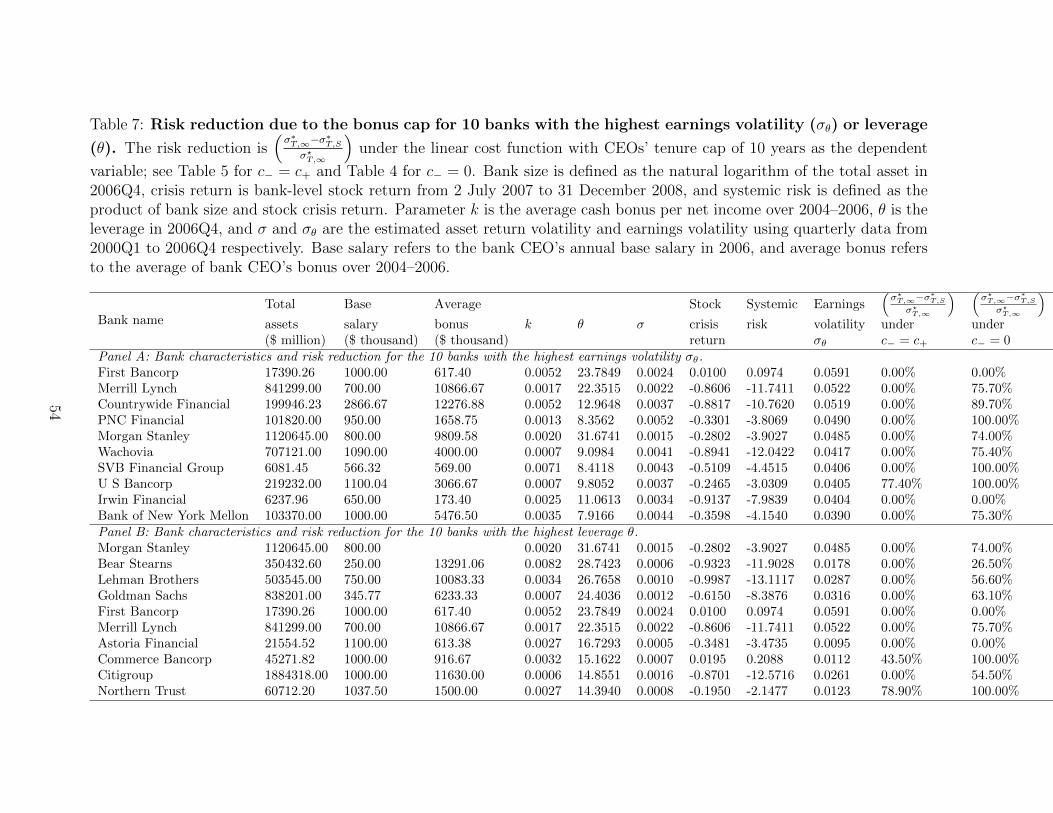
Table 7: Risk reduction due to the bonus cap for 10 banks with the highest earnings volatility (σθ) or leverage

(θ). The risk reduction is(σ∗T,∞−σ

∗T,S

σ?T,∞

)under the linear cost function with CEOs’ tenure cap of 10 years as the dependent

variable; see Table 5 for c− = c+ and Table 4 for c− = 0. Bank size is defined as the natural logarithm of the total asset in2006Q4, crisis return is bank-level stock return from 2 July 2007 to 31 December 2008, and systemic risk is defined as theproduct of bank size and stock crisis return. Parameter k is the average cash bonus per net income over 2004–2006, θ is theleverage in 2006Q4, and σ and σθ are the estimated asset return volatility and earnings volatility using quarterly data from2000Q1 to 2006Q4 respectively. Base salary refers to the bank CEO’s annual base salary in 2006, and average bonus refersto the average of bank CEO’s bonus over 2004–2006.

Bank nameTotal Base Average Stock Systemic Earnings

(σ?T,∞−σ∗T,S

σ?T,∞

) (σ?T,∞−σ∗T,S

σ?T,∞

)assets salary bonus k θ σ crisis risk volatility under under($ million) ($ thousand) ($ thousand) return σθ c− = c+ c− = 0

Panel A: Bank characteristics and risk reduction for the 10 banks with the highest earnings volatility σθ.First Bancorp 17390.26 1000.00 617.40 0.0052 23.7849 0.0024 0.0100 0.0974 0.0591 0.00% 0.00%Merrill Lynch 841299.00 700.00 10866.67 0.0017 22.3515 0.0022 -0.8606 -11.7411 0.0522 0.00% 75.70%Countrywide Financial 199946.23 2866.67 12276.88 0.0052 12.9648 0.0037 -0.8817 -10.7620 0.0519 0.00% 89.70%PNC Financial 101820.00 950.00 1658.75 0.0013 8.3562 0.0052 -0.3301 -3.8069 0.0490 0.00% 100.00%Morgan Stanley 1120645.00 800.00 9809.58 0.0020 31.6741 0.0015 -0.2802 -3.9027 0.0485 0.00% 74.00%Wachovia 707121.00 1090.00 4000.00 0.0007 9.0984 0.0041 -0.8941 -12.0422 0.0417 0.00% 75.40%SVB Financial Group 6081.45 566.32 569.00 0.0071 8.4118 0.0043 -0.5109 -4.4515 0.0406 0.00% 100.00%U S Bancorp 219232.00 1100.04 3066.67 0.0007 9.8052 0.0037 -0.2465 -3.0309 0.0405 77.40% 100.00%Irwin Financial 6237.96 650.00 173.40 0.0025 11.0613 0.0034 -0.9137 -7.9839 0.0404 0.00% 0.00%Bank of New York Mellon 103370.00 1000.00 5476.50 0.0035 7.9166 0.0044 -0.3598 -4.1540 0.0390 0.00% 75.30%Panel B: Bank characteristics and risk reduction for the 10 banks with the highest leverage θ.Morgan Stanley 1120645.00 800.00 0.0020 31.6741 0.0015 -0.2802 -3.9027 0.0485 0.00% 74.00%Bear Stearns 350432.60 250.00 13291.06 0.0082 28.7423 0.0006 -0.9323 -11.9028 0.0178 0.00% 26.50%Lehman Brothers 503545.00 750.00 10083.33 0.0034 26.7658 0.0010 -0.9987 -13.1117 0.0287 0.00% 56.60%Goldman Sachs 838201.00 345.77 6233.33 0.0007 24.4036 0.0012 -0.6150 -8.3876 0.0316 0.00% 63.10%First Bancorp 17390.26 1000.00 617.40 0.0052 23.7849 0.0024 0.0100 0.0974 0.0591 0.00% 0.00%Merrill Lynch 841299.00 700.00 10866.67 0.0017 22.3515 0.0022 -0.8606 -11.7411 0.0522 0.00% 75.70%Astoria Financial 21554.52 1100.00 613.38 0.0027 16.7293 0.0005 -0.3481 -3.4735 0.0095 0.00% 0.00%Commerce Bancorp 45271.82 1000.00 916.67 0.0032 15.1622 0.0007 0.0195 0.2088 0.0112 43.50% 100.00%Citigroup 1884318.00 1000.00 11630.00 0.0006 14.8551 0.0016 -0.8701 -12.5716 0.0261 0.00% 54.50%Northern Trust 60712.20 1037.50 1500.00 0.0027 14.3940 0.0008 -0.1950 -2.1477 0.0123 78.90% 100.00%

54

Appendix D Robustness checks

Table 8: Risk reductions for bonus caps and bonus deferrals — bonuses decrease equity value and the costparameters are equal. The bank-level bonus cap is the CEO’s annual salary in 2006 if the bonus interval is one year, thebonus cap is twice the CEO’s annual salary in 2006 if the bonus interval is two years, and the bonus cap is five times theCEO’s annual salary in 2006 if the bonus interval is five years. σ∗T,∞ is the estimated earnings volatility using the quarterlydata from 2000Q1 to 2006Q4. k is the cash bonus per net income in Panel A of Table 1. The average k during the period2004–2006 is used in this table. Panels A and B are the results by simulating the equity process that drops by the bonuspayment at each bonus payment time and between the payment times it follows (2). By σ∗T,∞ and (11), we get the parametersof the piecewise linear and quadratic cost functions, and then we set c− equal to c+ and c+ is the smallest cost parametervalue that satisfy the optimality condition (11) (not reported for brevity).

Case I: Bonus Case II: Bonus Case III: Bonus Case IV: Bonus Case V: Bonusinterval of 1 year interval of 2 years interval of 2 years interval of 5 years interval of 5 years

& bonus cap & no bonus cap & bonus cap & no bonus cap & bonus cap(σ∗T,∞−σ

∗T,S

σ∗T,∞

) (σ∗T,∞−σ

∗T/2,∞

σ∗T,∞

) (σ∗T,∞−σ

∗T/2,2S

σ∗T,∞

) (σ∗T,∞−σ

∗T/5,∞

σ∗T,∞

) (σ∗T,∞−σ

∗T/5,5S

σ∗T,∞

)Linear Quadratic Linear Quadratic Linear Quadratic Linear Quadratic Linear Quadratic

Panel A: T cap 10 yrs.Min 0.00% 0.00% 0.00% 0.00% 0.00% 0.00% 0.00% 0.00% -100.00% 0.00%Max 99.80% 5.20% 0.00% 0.00% 92.00% 3.30% 0.00% 0.00% 90.80% 1.80%Mean 14.14% 0.37% 0.00% 0.00% 10.12% 0.14% 0.00% 0.00% 2.06% 0.04%Std 31.06% 1.05% 0.00% 0.00% 26.18% 0.56% 0.00% 0.00% 22.92% 0.26%Panel B: T cap 15 yrs.Min 0.00% 0.00% -100.00% 0.00% -100.00% 0.00% 0.00% 0.00% -100.00% 0.00%Max 99.80% 8.10% 0.00% 0.00% 98.20% 4.80% 0.00% 0.00% 99.30% 2.20%Mean 18.78% 0.71% -16.47% 0.00% 3.98% 0.32% 0.00% 0.00% 5.06% 0.10%Std 35.32% 1.78% 37.31% 0.00% 44.74% 0.99% 0.00% 0.00% 27.75% 0.43%

55

Table 9: Cost function parameters — option grants. The earnings volatility isestimated using quarterly data from 2000Q1 to 2006Q4. The bank-level cost parametersare calculated from πT,∞(σθ + ∆σθ) + NπBS(σS + ∆σS)− F (∆σθ) = 0, where N is thenumber of option grants in 2006, πBS is the Black-Scholes value of the option grants, andσS is the stock volatility. The bonus value πT,∞ is calculated by using the average cashbonus per net income during the period 2004–2006 (average k in Panel A of Table 1).The stock volatility σS is estimated by using the daily stock price from 2000Q1 to2006Q4, and a linear relationship between the earnings volatility σθ is estimated asσS = a + 0.95 ∗ σθ to calculate the change of stock volatility ∆σS due to the changeof the earnings volatility σθ (see Vuolteenaho (2002)). Piecewise linear cost function:F (∆σθ) = c+I{∆σθ ≥ 0}∆σθ − c−I{∆σθ < 0}∆σθ, piecewise quadratic cost function:F (∆σθ) = c+I{∆σθ ≥ 0} (∆σθ)

2 + c−I{∆σθ < 0} (∆σθ)2. By σ∗T,∞ and (11), we get

the parameters of the piecewise linear and quadratic cost functions, where we select thesmallest cost parameter values that satisfy the optimality condition (11).

Cost function Linear function Quadratic functionparameters c+ c− c+ c−Panel A: T cap 10 yrs.Min 7 -109,567,032 1,069,560 -1,222,157,285Max 234,677,777 -7 2,980,930,256,815 -1,069Mean 25,281,227 -6,916,738 308,528,444,812 -99,230,871Std 46,847,220 16,273,853 574,694,368,292 195,202,653Panel B: T cap 15 yrs.Min 8 -51,715,483 1,174,804 -996,267,654Max 358,934,953 0 5,008,435,539,163 -2Mean 23,520,104 -3,251,710 323,941,895,933 -77,737,372Std 64,136,152 9,356,435 920,423,621,677 215,813,232

56

Table 10: Risk reductions for bonus caps and bonus deferrals — option grants and the cost parameters areequal. The bank-level bonus cap is the CEO’s annual salary in 2006 if the bonus interval is one year, the bonus cap is twicethe CEO’s annual salary in 2006 if the bonus interval is two years, and the bonus cap is five times the CEO’s annual salaryin 2006 if the bonus interval is five years. σ∗T,∞ is the estimated earnings volatility using the quarterly data from 2000Q1 to2006Q4. k is the cash bonus per net income in Panel A of Table 1. The average k during the period 2004–2006 is used inthis table. The banker’s objective is to maximize the net payoff πn,M(σθ + ∆σθ) + NπBS(σS + ∆σS) − F (∆σθ), where Nis the number of option grants in 2006, πBS is the Black-Scholes value of the option grants, and σS is the stock volatility.The bonus value πT,∞ is calculated by using the average cash bonus per net income during the period 2004–2006 (averagek in Panel A of Table 1). The stock volatility σS is estimated by using the daily stock price from 2000Q1 to 2006Q4, anda linear relationship between the earnings volatility σθ is estimated as σS = a + 0.95 ∗ σθ to calculate the change of stockvolatility ∆σS due to the change of the earnings volatility σθ (see Vuolteenaho (2002)). The parameters of the piecewiselinear and quadratic cost functions are reported in Table 9. To calculate the risk reduction, we set c− equal to c+ in thecost functions. Piecewise linear cost function: F (∆σθ) = c+I{∆σθ ≥ 0}∆σθ − c−I{∆σθ < 0}∆σθ, piecewise quadratic costfunction: F (∆σθ) = c+I{∆σθ ≥ 0} (∆σθ)

2 + c−I{∆σθ < 0} (∆σθ)2.

Case I: Bonus Case II: Bonus Case III: Bonus Case IV: Bonus Case V: Bonusinterval of 1 year interval of 2 years interval of 2 years interval of 5 years interval of 5 years

& bonus cap & no bonus cap & bonus cap & no bonus cap & bonus cap(σ∗T,∞−σ

∗T,S

σ∗T,∞

) (σ∗T,∞−σ

∗T/2,∞

σ∗T,∞

) (σ∗T,∞−σ

∗T/2,2S

σ∗T,∞

) (σ∗T,∞−σ

∗T/5,∞

σ∗T,∞

) (σ∗T,∞−σ

∗T/5,5S

σ∗T,∞

)Linear Quadratic Linear Quadratic Linear Quadratic Linear Quadratic Linear Quadratic

Panel A: T cap 10 yrs.Min 0.00% 0.00% 0.00% 0.00% 0.00% 0.00% 0.00% 0.00% 0.00% 0.00%Max 82.80% 0.80% 0.00% 0.00% 63.40% 0.30% 0.00% 0.00% 0.00% 0.10%Mean 9.69% 0.05% 0.00% 0.00% 1.73% 0.02% 0.00% 0.00% 0.00% 0.01%Std 23.89% 0.14% 0.00% 0.00% 9.52% 0.07% 0.00% 0.00% 0.00% 0.03%Panel B: T cap 15 yrs.Min 0.00% 0.00% 0.00% 0.00% 0.00% 0.00% 0.00% 0.00% 0.00% 0.00%Max 100.00% 100.00% 0.00% 0.00% 100.00% 100.00% 0.00% 0.00% 91.20% 75.70%Mean 27.65% 17.88% 0.00% 0.00% 19.55% 13.19% 0.00% 0.00% 9.49% 6.82%Std 39.38% 33.48% 0.00% 0.00% 34.70% 28.09% 0.00% 0.00% 23.34% 17.56%

57

Table 11: Cost function parameters — internal bonus cap. The earnings volatilityis estimated using quarterly data from 2000Q1 to 2006Q4. Different from the optimalitycondition (11), to calculate the bank-level cost parameters, we assume that the internalbonus cap is five times the annual salary in 2006 if the bonus is no more than fivetimes the annual salary in 2006, whereas if the bonus is more than five times the annualsalary in 2006, we assume that the internal bonus cap is infinite in 2006. Besides, weassume that the bonus is paid every year. The optimality condition is similar to (11) butwith the internal bonus cap. The bank-level cost parameters are calculated using theaverage cash bonus per net income during the period 2004–2006 (average k in Panel Aof Table 1). Piecewise linear cost function: F (∆σθ) = c+I{∆σθ ≥ 0}∆σθ − c−I{∆σθ <0}∆σθ, piecewise quadratic cost function: F (∆σθ) = c+I{∆σθ ≥ 0} (∆σθ)

2+c−I{∆σθ <0} (∆σθ)

2. We select the smallest cost parameter values that satisfy the above optimalitycondition.

Cost function Linear function Quadratic functionparameters c+ c− c+ c−Panel A: T cap 10 yrs.Min -63,535,115 -48,684,793 -1,309,339,014 -933,524,489Max 239,289,959 7,167,380,914 3,338,956,682,603 2,404,864,434,231Mean 10,111,538 167,941,696 161,262,343,043 86,137,536,890Std 38,465,334 905,393,764 539,244,064,791 368,876,418,781Panel B: T cap 15 yrs.Min -83,428,477 -73,027,190 -1,719,303,709 -1,400,286,734Max 358,934,939 8,492,198,084 5,008,435,023,895 3,275,347,310,215Mean 13,930,819 206,184,177 229,112,646,293 136,935,206,853Std 56,775,157 1,085,803,710 785,145,102,131 548,334,727,710

58

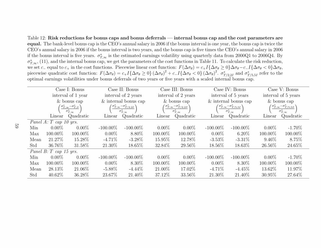
Table 12: Risk reductions for bonus caps and bonus deferrals — internal bonus cap and the cost parameters areequal. The bank-level bonus cap is the CEO’s annual salary in 2006 if the bonus interval is one year, the bonus cap is twice theCEO’s annual salary in 2006 if the bonus interval is two years, and the bonus cap is five times the CEO’s annual salary in 2006if the bonus interval is five years. σ∗T,∞ is the estimated earnings volatility using quarterly data from 2000Q1 to 2006Q4. Byσ∗T,∞, (11), and the internal bonus cap, we get the parameters of the cost functions in Table 11. To calculate the risk reduction,we set c− equal to c+ in the cost functions. Piecewise linear cost function: F (∆σθ) = c+I{∆σθ ≥ 0}∆σθ−c−I{∆σθ < 0}∆σθ,piecewise quadratic cost function: F (∆σθ) = c+I{∆σθ ≥ 0} (∆σθ)

2 + c−I{∆σθ < 0} (∆σθ)2. σ∗T/2,2I and σ∗T/5,5I refer to the

optimal earnings volatilities under bonus deferrals of two years or five years with a scaled internal bonus cap.

Case I: Bonus Case II: Bonus Case III: Bonus Case IV: Bonus Case V: Bonusinterval of 1 year interval of 2 years interval of 2 years interval of 5 years interval of 5 years

& bonus cap & internal bonus cap & bonus cap & internal bonus cap & bonus cap(σ∗T,∞−σ

∗T,S

σ?T,∞

) (σ∗T,∞−σ

∗T/2,2I

σ∗T,∞

) (σ∗T,∞−σ

∗T/2,2S

σ∗T,∞

) (σ∗T,∞−σ

∗T/5,5I

σ∗T,∞

) (σ∗T,∞−σ

∗T/5,5S

σ∗T,∞

)Linear Quadratic Linear Quadratic Linear Quadratic Linear Quadratic Linear Quadratic

Panel A: T cap 10 yrs.Min 0.00% 0.00% -100.00% -100.00% 0.00% 0.00% -100.00% -100.00% 0.00% -1.70%Max 100.00% 100.00% 0.00% 8.80% 100.00% 100.00% 0.00% 6.20% 100.00% 100.00%Mean 21.27% 15.28% -4.71% -3.28% 15.95% 12.78% -3.53% -3.31% 9.46% 8.75%Std 36.76% 31.58% 21.30% 18.65% 32.84% 29.56% 18.56% 18.63% 26.56% 24.65%Panel B: T cap 15 yrs.Min 0.00% 0.00% -100.00% -100.00% 0.00% 0.00% -100.00% -100.00% 0.00% -1.70%Max 100.00% 100.00% 0.00% 8.30% 100.00% 100.00% 0.00% 8.30% 100.00% 100.00%Mean 28.13% 21.06% -5.88% -4.44% 21.00% 17.02% -4.71% -4.45% 13.62% 11.97%Std 40.62% 36.28% 23.67% 21.40% 37.12% 33.56% 21.30% 21.40% 30.95% 27.64%

59

Table 13: Risk reductions for bonus caps and bonus deferrals — augmented fixed salary and the cost pa-rameters are equal. The CEO’s annual base salary has been augmented as follows: we first calculate the total expecteddiscounted value of the bonuses that are paid every year without the bonus cap and the annual base salary during theCEO’s tenure cap of 10 or 15 years, denoted as K10 or K15, for example, K10 =

∑T cap 10i=1 exp(−(i − 1)r)πT,∞ + S, where

S is the actual base salary in 2006; then we consider the total value of the bonuses and the augmented base salary duringthe CEO’s tenure, which is K ′10 or K ′15 under the tenure cap of 10 or 15 years, where bonuses are paid every year andcapped at this augmented base salary, for example, K ′10 =

∑T cap 10i=1 exp(−(i − 1)r)πT,S′ + S ′, where S ′ is the augmented

base salary such that K10 = K ′10. The bank-level bonus cap is the CEO’s annual augmented base salary in 2006 if thebonus interval is one year, the bonus cap is twice the CEO’s annual augmented base salary in 2006 if the bonus intervalis two years, and the bonus cap is five times the CEO’s annual augmented base salary in 2006 if the bonus interval is fiveyears. σ∗T,∞ is the estimated earnings volatility using quarterly data from 2000Q1 to 2006Q4. By σ∗T,∞ and (11), we get theparameters of the cost functions (not reported for brevity). To calculate the risk reduction, we set c− equal to c+ in thecost functions. Piecewise linear cost function: F (∆σθ) = c+I{∆σθ ≥ 0}∆σθ − c−I{∆σθ < 0}∆σθ, piecewise quadratic costfunction: F (∆σθ) = c+I{∆σθ ≥ 0} (∆σθ)

2 + c−I{∆σθ < 0} (∆σθ)2.

Case I: Bonus Case II: Bonus Case III: Bonus Case IV: Bonus Case V: Bonusinterval of 1 year interval of 2 years interval of 2 years interval of 5 years interval of 5 years

& bonus cap & no bonus cap & bonus cap & no bonus cap & bonus cap(σ∗T,∞−σ

∗T,S

σ?T,∞

) (σ∗T,∞−σ

∗T/2,∞

σ∗T,∞

) (σ∗T,∞−σ

∗T/2,2S

σ∗T,∞

) (σ∗T,∞−σ

∗T/5,∞

σ∗T,∞

) (σ∗T,∞−σ

∗T/5,5S

σ∗T,∞

)Linear Quadratic Linear Quadratic Linear Quadratic Linear Quadratic Linear Quadratic

Panel A: T cap 10 yrs.Min 0.00% 0.00% 0.00% 0.00% 0.00% 0.00% 0.00% 0.00% 0.00% 0.00%Max 100.00% 100.00% 0.00% 0.00% 100.00% 100.00% 0.00% 0.00% 81.40% 79.60%Mean 19.72% 12.01% 0.00% 0.00% 12.81% 9.91% 0.00% 0.00% 5.89% 5.33%Std 33.91% 27.75% 0.00% 0.00% 29.25% 25.60% 0.00% 0.00% 18.53% 15.96%Panel B: T cap 15 yrs.Min 0.00% 0.00% 0.00% 0.00% 0.00% 0.00% 0.00% 0.00% 0.00% 0.00%Max 100.00% 100.00% 0.00% 0.00% 100.00% 100.00% 0.00% 0.00% 100.00% 100.00%Mean 25.14% 17.08% 0.00% 0.00% 16.75% 12.83% 0.00% 0.00% 10.52% 8.20%Std 37.48% 32.46% 0.00% 0.00% 33.15% 28.43% 0.00% 0.00% 26.73% 21.35%

60

Table 14: Jump size parameters for the jump-diffusion process. σθ 2006 is theearnings volatility estimated using quarterly data from 2000Q1 to 2006Q4. The equitydynamics follow the jump-diffusion process dA(t)

A(t)= (r−λu)dt+σdW (t)+udN(t), where

u ∈ [−1, 0] is the jump size and λ is the intensity of the Poisson process N(t). In theabove jump-diffusion process, the expected growth rate of the jump-diffusion processis r, the same as the drift in (2). We also match the instantaneous volatility of thejump-diffusion process with the Wiener process in (2) as σ2

θ = σ2 +λu2. We fix λ = 0.1.Further, we assume that at the end of 2006, σ = 0, to solve the equilibrium jump size uin 2006 as u = − σθ√

λ.

Jump size u, 2006Min -0.2339Max -0.0106Mean -0.0522Std 0.0430

61

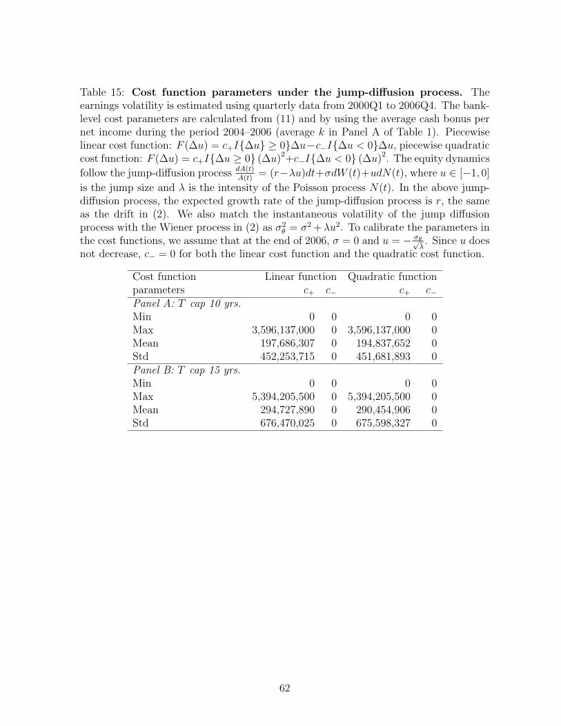
Table 15: Cost function parameters under the jump-diffusion process. Theearnings volatility is estimated using quarterly data from 2000Q1 to 2006Q4. The bank-level cost parameters are calculated from (11) and by using the average cash bonus pernet income during the period 2004–2006 (average k in Panel A of Table 1). Piecewiselinear cost function: F (∆u) = c+I{∆u} ≥ 0}∆u−c−I{∆u < 0}∆u, piecewise quadraticcost function: F (∆u) = c+I{∆u ≥ 0} (∆u)2+c−I{∆u < 0} (∆u)2. The equity dynamics

follow the jump-diffusion process dA(t)A(t)

= (r−λu)dt+σdW (t)+udN(t), where u ∈ [−1, 0]

is the jump size and λ is the intensity of the Poisson process N(t). In the above jump-diffusion process, the expected growth rate of the jump-diffusion process is r, the sameas the drift in (2). We also match the instantaneous volatility of the jump diffusionprocess with the Wiener process in (2) as σ2

θ = σ2 +λu2. To calibrate the parameters inthe cost functions, we assume that at the end of 2006, σ = 0 and u = − σθ√

λ. Since u does

not decrease, c− = 0 for both the linear cost function and the quadratic cost function.

Cost function Linear function Quadratic functionparameters c+ c− c+ c−Panel A: T cap 10 yrs.Min 0 0 0 0Max 3,596,137,000 0 3,596,137,000 0Mean 197,686,307 0 194,837,652 0Std 452,253,715 0 451,681,893 0Panel B: T cap 15 yrs.Min 0 0 0 0Max 5,394,205,500 0 5,394,205,500 0Mean 294,727,890 0 290,454,906 0Std 676,470,025 0 675,598,327 0

62

Table 16: Jump size increments for bonus caps and bonus deferrals. The bank-level bonus cap is the CEO’s annualsalary in 2006 if the bonus interval is one year, the bonus cap is twice the CEO’s annual salary in 2006 if the bonus intervalis two years, and the bonus cap is five times the CEO’s annual salary in 2006 if the bonus interval is five years. σ∗T,∞ is theestimated earnings volatility using the quarterly data from 2000Q1 to 2006Q4. k is the cash bonus per net income in Panel Aof Table 1. The average k during the period 2004–2006 is used in this table. The equity dynamics follow the jump-diffusionprocess dA(t)

A(t)= (r − λu)dt + σdW (t) + udN(t), where u ∈ [−1, 0] is the jump size and λ is the intensity of the Poisson

process N(t). In the above jump-diffusion process, the expected growth rate of the jump-diffusion process is r, the same asthe drift in (2). We also match the instantaneous volatility of the jump-diffusion process with the Wiener process in (2) asσ2θ = σ2 +λu2. Similar to the optimality condition in (11), the banker’s objective is to maximize πn,M(u∗T,∞+ ∆u)−F (∆u),

where u∗T,∞ is the equilibrium jump size; see Table 14, and the optimal jump size is denoted as u∗n,M . The parameters of thepiecewise linear and quadratic cost functions in terms of change of jump size u are in Table 15.

Case I: Bonus Case II: Bonus Case III: Bonus Case IV: Bonus Case V: Bonusinterval of 1 year interval of 2 years interval of 2 years interval of 5 years interval of 5 years

& bonus cap & no bonus cap & bonus cap & no bonus cap & bonus cap(u∗T,∞−u

∗T,S

u∗T,∞

) (u∗T,∞−u

∗T/2,∞

u∗T,∞

) (u∗T,∞−u

∗T/2,2S

u∗T,∞

) (u∗T,∞−u

∗T/5,∞

u∗T,∞

) (u∗T,∞−u

∗T/5,5S

u∗T,∞

)Linear Quadratic Linear Quadratic Linear Quadratic Linear Quadratic Linear Quadratic

Panel A: T cap 10 yrs.Min 0.00% 0.00% 0.00% 0.00% 0.00% 0.00% 0.00% 0.00% 0.00% 0.00%Max 0.00% 3.90% 0.00% 0.00% 0.00% 0.00% 0.00% 0.00% 0.00% 0.00%Mean 0.00% 0.05% 0.00% 0.00% 0.00% 0.00% 0.00% 0.00% 0.00% 0.00%Std 0.00% 0.44% 0.00% 0.00% 0.00% 0.00% 0.00% 0.00% 0.00% 0.00%Panel B: T cap 15 yrs.Min 0.00% 0.00% 0.00% 0.00% 0.00% 0.00% 0.00% 0.00% 0.00% 0.00%Max 0.00% 3.90% 0.00% 0.00% 0.00% 0.10% 0.00% 0.00% 0.00% 0.10%Mean 0.00% 0.05% 0.00% 0.00% 0.00% 0.00% 0.00% 0.00% 0.00% 0.00%Std 0.00% 0.44% 0.00% 0.00% 0.00% 0.01% 0.00% 0.00% 0.00% 0.01%

63

Table 17: Cost function parameters for the risk averse banker. The bankeris assumed to be risk averse and her objective is to maximize the net expected util-

ity defined as Un,M(σθ + ∆σθ) = E

[W 1−γn,M (σθ+∆σθ)

1−γ

]− F (∆σθ), where Wn,M(σθ) =∑n

i min[kmax[A(i∆)−A((i−1)∆), 0],M ], we set γ = 0.5, and A(t) is the equity processin (3).30 Instead of (11), the bank-level cost parameters are calculated by the optimalitycondition arg max∆σθ≥−σθ UT,∞(σ∗T,∞ + ∆σθ) = 0, where σ∗T,∞ is the estimated earningsvolatility using quarterly data from 2000Q1 to 2006Q4, and by using the average cashbonus per net income during the period 2004–2006 (average k in Panel A of Table 1). Thesmallest cost parameters that satisfy the above optimality condition are reported in thistable. Piecewise linear cost function: F (∆u) = c+I{∆u} ≥ 0}∆u − c−I{∆u < 0}∆u,piecewise quadratic cost function: F (∆u) = c+I{∆u ≥ 0} (∆u)2 + c−I{∆u < 0} (∆u)2.

Cost function Linear function Quadratic functionparameters c+ c− c+ c−Panel A: T cap 10 yrs.Min -1,225 -5,353 -122,299 -102,656Max 25,665 3,128 396,625,603 174,372,442Mean 2,718 61 36,448,116 28,109,437Std 6,311 1,264 88,548,050 28,118,139Panel B: T cap 15 yrs.Min -1,225 -7,475 -92,126 -143,349Max 32,014 3,128 508,104,661 174,372,442Mean 3,474 -151 47,369,055 21,607,904Std 7,649 1,539 111,058,726 25,846,107

30Bankers’ risk aversion is captured by γ > 0, γ 6= 1. Parameter γ = 2 is used, e.g., in Mehra andPrescott (1985) and Keppo and Petajisto (2014). We use γ = 0.5 instead in order to have a relativelylarge utility value to avoid the potential numerical errors in the risk reduction simulation. Note thatunder γ = 0.5, the utility function is concave and, thus, the banker is risk averse.

64

Table 18: Risk reductions for bonus caps and bonus deferrals — risk averse banker and c− is nonnegative. Thebanker is assumed to be risk averse and her objective is to maximize the net expected utility defined as Un,M(σθ + ∆σθ) =

E

[W 1−γn,M (σθ+∆σθ)

1−γ

]− F (∆σθ), where Wn,M(σθ) =

∑ni min[kmax[A(i∆)−A((i− 1)∆), 0],M ], we set γ = 0.5, and A(t) is the

equity process in (3). The bank-level bonus cap is the CEO’s annual salary in 2006 if the bonus interval is one year, the bonuscap is twice the CEO’s annual salary in 2006 if the bonus interval is two years, and the bonus cap is five times the CEO’sannual salary in 2006 if the bonus interval is five years. σ∗T,∞ is the estimated earnings volatility using quarterly data from2000Q1 to 2006Q4. To calculate the risk reduction, we set c− = max(cs−, 0) and c+ = cs+ in the cost functions, where cs+ andcs− are the cost parameters in Table 17. Piecewise linear cost function: F (∆σθ) = c+I{∆σθ ≥ 0}∆σθ − c−I{∆σθ < 0}∆σθ,piecewise quadratic cost function: F (∆σθ) = c+I{∆σθ ≥ 0} (∆σθ)

2 + c−I{∆σθ < 0} (∆σθ)2.

Case I: Bonus Case II: Bonus Case III: Bonus Case IV: Bonus Case V: Bonusinterval of 1 year interval of 2 years interval of 2 years interval of 5 years interval of 5 years

& bonus cap & no bonus cap & bonus cap & no bonus cap & bonus cap(σ∗T,∞−σ

∗T,S

σ?T,∞

) (σ∗T,∞−σ

∗T/2,∞

σ∗T,∞

) (σ∗T,∞−σ

∗T/2,2S

σ∗T,∞

) (σ∗T,∞−σ

∗T/5,∞

σ∗T,∞

) (σ∗T,∞−σ

∗T/5,5S

σ∗T,∞

)Linear Quadratic Linear Quadratic Linear Quadratic Linear Quadratic Linear Quadratic

Panel A: T cap 10 yrs.Min 0.00% 0.00% 0.00% 0.00% 0.00% 0.00% 0.00% 0.00% 0.00% 0.00%Max 100.00% 100.00% 93.70% 93.70% 100.00% 100.00% 92.40% 92.40% 100.00% 100.00%Mean 25.37% 14.03% 18.48% 17.37% 27.27% 18.56% 18.72% 17.75% 19.90% 16.06%Std 40.20% 33.14% 35.13% 33.65% 40.04% 35.79% 34.54% 33.36% 36.70% 34.33%Panel B: T cap 15 yrs.Min 0.00% 0.00% 0.00% 0.00% 0.00% 0.00% 0.00% 0.00% 0.00% 0.00%Max 100.00% 100.00% 93.80% 93.80% 100.00% 100.00% 98.70% 98.70% 100.00% 100.00%Mean 34.95% 16.37% 20.53% 19.85% 34.74% 20.56% 23.74% 22.61% 27.39% 18.67%Std 43.35% 35.32% 37.49% 36.67% 43.07% 38.09% 40.78% 39.61% 41.14% 37.30%

65

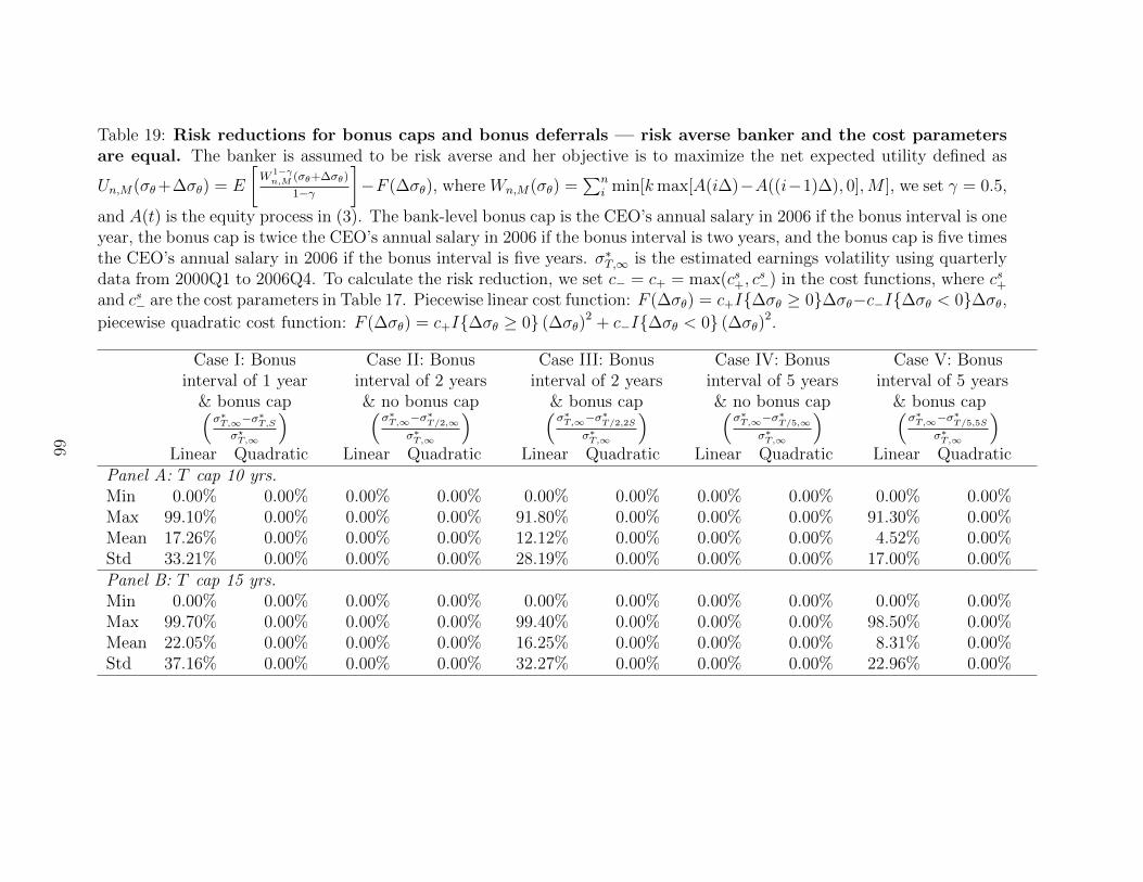
Table 19: Risk reductions for bonus caps and bonus deferrals — risk averse banker and the cost parametersare equal. The banker is assumed to be risk averse and her objective is to maximize the net expected utility defined as

Un,M(σθ+∆σθ) = E

[W 1−γn,M (σθ+∆σθ)

1−γ

]−F (∆σθ), where Wn,M(σθ) =

∑ni min[kmax[A(i∆)−A((i−1)∆), 0],M ], we set γ = 0.5,

and A(t) is the equity process in (3). The bank-level bonus cap is the CEO’s annual salary in 2006 if the bonus interval is oneyear, the bonus cap is twice the CEO’s annual salary in 2006 if the bonus interval is two years, and the bonus cap is five timesthe CEO’s annual salary in 2006 if the bonus interval is five years. σ∗T,∞ is the estimated earnings volatility using quarterlydata from 2000Q1 to 2006Q4. To calculate the risk reduction, we set c− = c+ = max(cs+, c

s−) in the cost functions, where cs+

and cs− are the cost parameters in Table 17. Piecewise linear cost function: F (∆σθ) = c+I{∆σθ ≥ 0}∆σθ−c−I{∆σθ < 0}∆σθ,piecewise quadratic cost function: F (∆σθ) = c+I{∆σθ ≥ 0} (∆σθ)

2 + c−I{∆σθ < 0} (∆σθ)2.

Case I: Bonus Case II: Bonus Case III: Bonus Case IV: Bonus Case V: Bonusinterval of 1 year interval of 2 years interval of 2 years interval of 5 years interval of 5 years

& bonus cap & no bonus cap & bonus cap & no bonus cap & bonus cap(σ∗T,∞−σ

∗T,S

σ?T,∞

) (σ∗T,∞−σ

∗T/2,∞

σ∗T,∞

) (σ∗T,∞−σ

∗T/2,2S

σ∗T,∞

) (σ∗T,∞−σ

∗T/5,∞

σ∗T,∞

) (σ∗T,∞−σ

∗T/5,5S

σ∗T,∞

)Linear Quadratic Linear Quadratic Linear Quadratic Linear Quadratic Linear Quadratic

Panel A: T cap 10 yrs.Min 0.00% 0.00% 0.00% 0.00% 0.00% 0.00% 0.00% 0.00% 0.00% 0.00%Max 99.10% 0.00% 0.00% 0.00% 91.80% 0.00% 0.00% 0.00% 91.30% 0.00%Mean 17.26% 0.00% 0.00% 0.00% 12.12% 0.00% 0.00% 0.00% 4.52% 0.00%Std 33.21% 0.00% 0.00% 0.00% 28.19% 0.00% 0.00% 0.00% 17.00% 0.00%Panel B: T cap 15 yrs.Min 0.00% 0.00% 0.00% 0.00% 0.00% 0.00% 0.00% 0.00% 0.00% 0.00%Max 99.70% 0.00% 0.00% 0.00% 99.40% 0.00% 0.00% 0.00% 98.50% 0.00%Mean 22.05% 0.00% 0.00% 0.00% 16.25% 0.00% 0.00% 0.00% 8.31% 0.00%Std 37.16% 0.00% 0.00% 0.00% 32.27% 0.00% 0.00% 0.00% 22.96% 0.00%

66

Appendix E Further robustness checks

Table 20: Risk reductions for bonus caps and bonus deferrals with earnings volatility estimates includingyears 2007 and 2008 — the smallest cost parameters. The bank-level bonus cap is the CEO’s annual salary in 2006if the bonus interval is one year, the bonus cap is twice the CEO’s annual salary in 2006 if the bonus interval is two years,and the bonus cap is five times the CEO’s annual salary in 2006 if the bonus interval is five years. σ∗T,∞ is the estimatedearnings volatility using quarterly data from 2000Q1 to 2008Q4. By σ∗T,∞ and (11), we get the smallest parameters of thecost functions (not reported for brevity). Piecewise linear cost function: F (∆σθ) = c+I{∆σθ ≥ 0}∆σθ− c−I{∆σθ < 0}∆σθ,piecewise quadratic cost function: F (∆σθ) = c+I{∆σθ ≥ 0} (∆σθ)

2 + c−I{∆σθ < 0} (∆σθ)2.

Case I: Bonus Case II: Bonus Case III: Bonus Case IV: Bonus Case V: Bonusinterval of 1 year interval of 2 years interval of 2 years interval of 5 years interval of 5 years

& bonus cap & no bonus cap & bonus cap & no bonus cap & bonus cap(σ∗T,∞−σ

∗T,S

σ?T,∞

) (σ∗T,∞−σ

∗T/2,∞

σ∗T,∞

) (σ∗T,∞−σ

∗T/2,2S

σ∗T,∞

) (σ∗T,∞−σ

∗T/5,∞

σ∗T,∞

) (σ∗T,∞−σ

∗T/5,5S

σ∗T,∞

)Linear Quadratic Linear Quadratic Linear Quadratic Linear Quadratic Linear Quadratic

Panel A: T cap 10 yrs.Min 0.00% 0.00% 0.00% 0.00% 0.00% 0.00% 0.00% 0.00% 0.00% 0.00%Max 100.00% 100.00% 100.00% 100.00% 100.00% 100.00% 100.00% 100.00% 100.00% 100.00%Mean 63.52% 63.52% 70.59% 70.59% 74.06% 74.04% 70.59% 70.59% 73.81% 73.76%Std 48.42% 48.41% 45.83% 45.83% 44.03% 44.02% 45.83% 45.83% 43.97% 43.97%Panel B: T cap 15 yrs.Min 0.00% 0.00% 0.00% 0.00% 0.00% 0.00% 0.00% 0.00% 0.00% 0.00%Max 100.00% 100.00% 100.00% 100.00% 100.00% 100.00% 100.00% 100.00% 100.00% 100.00%Mean 67.97% 68.00% 70.59% 70.59% 75.29% 75.29% 70.59% 70.59% 74.87% 74.87%Std 46.71% 46.72% 45.83% 45.83% 45.83% 45.83% 45.83% 45.83% 43.23% 43.23%

67

Table 21: Risk reductions for bonus caps and bonus deferrals with earnings volatility estimates includingyears 2007 and 2008 — the cost parameter c− is zero. The bank-level bonus cap is the CEO’s annual salary in 2006if the bonus interval is one year, the bonus cap is twice the CEO’s annual salary in 2006 if the bonus interval is two years,and the bonus cap is five times the CEO’s annual salary in 2006 if the bonus interval is five years. σ∗T,∞ is the estimatedearnings volatility using quarterly data from 2000Q1 to 2008Q4. By σ∗T,∞ and (11), we get the smallest parameters of thecost functions (not reported for brevity). Instead of the smallest cost c−, we set c− = 0 to calculate the risk reduction.Piecewise linear cost function: F (∆σθ) = c+I{∆σθ ≥ 0}∆σθ − c−I{∆σθ < 0}∆σθ, piecewise quadratic cost function:F (∆σθ) = c+I{∆σθ ≥ 0} (∆σθ)

2 + c−I{∆σθ < 0} (∆σθ)2.

Case I: Bonus Case II: Bonus Case III: Bonus Case IV: Bonus Case V: Bonusinterval of 1 year interval of 2 years interval of 2 years interval of 5 years interval of 5 years

& bonus cap & no bonus cap & bonus cap & no bonus cap & bonus cap(σ∗T,∞−σ

∗T,S

σ?T,∞

) (σ∗T,∞−σ

∗T/2,∞

σ∗T,∞

) (σ∗T,∞−σ

∗T/2,2S

σ∗T,∞

) (σ∗T,∞−σ

∗T/5,∞

σ∗T,∞

) (σ∗T,∞−σ

∗T/5,5S

σ∗T,∞

)Linear Quadratic Linear Quadratic Linear Quadratic Linear Quadratic Linear Quadratic

Panel A: T cap 10 yrs.Min 0.00% 0.00% 0.00% 0.00% 0.00% 0.00% 0.00% 0.00% 0.00% 0.00%Max 100.00% 100.00% 0.00% 0.00% 100.00% 100.00% 0.00% 0.00% 100.00% 100.00%Mean 36.09% 36.09% 0.00% 0.00% 35.95% 35.94% 0.00% 0.00% 35.66% 35.60%Std 46.17% 46.17% 0.00% 0.00% 45.62% 45.60% 0.00% 0.00% 44.74% 44.69%Panel B: T cap 15 yrs.Min 0.00% 0.00% 0.00% 0.00% 0.00% 0.00% 0.00% 0.00% 0.00% 0.00%Max 100.00% 100.00% 0.00% 0.00% 100.00% 100.00% 0.00% 0.00% 100.00% 100.00%Mean 45.10% 45.73% 0.00% 0.00% 43.04% 43.04% 0.00% 0.00% 42.06% 42.06%Std 47.71% 47.73% 0.00% 0.00% 47.31% 47.31% 0.00% 0.00% 46.02% 46.02%

68

Table 22: Risk reductions for bonus caps and bonus deferrals with earnings volatility estimates includingyears 2007 and 2008 — the cost parameters are equal. The bank-level bonus cap is the CEO’s annual salary in 2006if the bonus interval is one year, the bonus cap is twice the CEO’s annual salary in 2006 if the bonus interval is two years,and the bonus cap is five times the CEO’s annual salary in 2006 if the bonus interval is five years. σ∗T,∞ is the estimatedearnings volatility using quarterly data from 2000Q1 to 2008Q4. By σ∗T,∞ and (11), we get the smallest parameters ofthe cost functions (not reported for brevity). Instead of the smallest cost c−, we set c− equal to c+ to calculate the riskreduction. Piecewise linear cost function: F (∆σθ) = c+I{∆σθ ≥ 0}∆σθ − c−I{∆σθ < 0}∆σθ, piecewise quadratic costfunction: F (∆σθ) = c+I{∆σθ ≥ 0} (∆σθ)

2 + c−I{∆σθ < 0} (∆σθ)2.

Case I: Bonus Case II: Bonus Case III: Bonus Case IV: Bonus Case V: Bonusinterval of 1 year interval of 2 years interval of 2 years interval of 5 years interval of 5 years

& bonus cap & no bonus cap & bonus cap & no bonus cap & bonus cap(σ∗T,∞−σ

∗T,S

σ?T,∞

) (σ∗T,∞−σ

∗T/2,∞

σ∗T,∞

) (σ∗T,∞−σ

∗T/2,2S

σ∗T,∞

) (σ∗T,∞−σ

∗T/5,∞

σ∗T,∞

) (σ∗T,∞−σ

∗T/5,5S

σ∗T,∞

)Linear Quadratic Linear Quadratic Linear Quadratic Linear Quadratic Linear Quadratic

Panel A: T cap 10 yrs.Min 0.00% 0.00% 0.00% 0.00% 0.00% 0.00% 0.00% 0.00% 0.00% 0.00%Max 100.00% 98.90% 0.00% 0.00% 100.00% 95.20% 0.00% 0.00% 83.00% 82.60%Mean 8.79% 2.43% 0.00% 0.00% 3.68% 2.24% 0.00% 0.00% 1.67% 1.66%Std 24.07% 15.06% 0.00% 0.00% 16.59% 14.22% 0.00% 0.00% 10.96% 10.90%Panel B: T cap 15 yrs.Min 0.00% 0.00% 0.00% 0.00% 0.00% 0.00% 0.00% 0.00% 0.00% 0.00%Max 100.00% 100.00% 0.00% 0.00% 100.00% 98.10% 0.00% 0.00% 98.40% 81.40%Mean 10.18% 3.33% 0.00% 0.00% 4.96% 2.33% 0.00% 0.00% 3.08% 1.99%Std 26.53% 16.73% 0.00% 0.00% 19.12% 14.40% 0.00% 0.00% 16.24% 12.40%

69

Table 23: Risk reductions for bonus caps and bonus deferrals with earnings volatility estimates includingyears 2007 and 2008 — internal bonus cap and the cost parameters are equal. The bank-level bonus cap is theCEO’s annual salary in 2006 if the bonus interval is one year, the bonus cap is twice the CEO’s annual salary in 2006 ifthe bonus interval is two years, and the bonus cap is five times the CEO’s annual salary in 2006 if the bonus interval is fiveyears. σ∗T,∞ is the estimated earnings volatility using quarterly data from 2000Q1 to 2008Q4. By σ∗T,∞, (11), and the internalbonus cap, we get the parameters of the cost functions (not reported for brevity). To calculate the risk reduction, we setc− equal to c+ in the cost functions. Piecewise linear cost function: F (∆σθ) = c+I{∆σθ ≥ 0}∆σθ − c−I{∆σθ < 0}∆σθ,piecewise quadratic cost function: F (∆σθ) = c+I{∆σθ ≥ 0} (∆σθ)

2 + c−I{∆σθ < 0} (∆σθ)2. σ∗T/2,2I and σ∗T/5,5I refer to the

optimal earnings volatilities under bonus deferrals of two years or five years with a scaled internal bonus cap.

Case I: Bonus Case II: Bonus Case III: Bonus Case IV: Bonus Case V: Bonusinterval of 1 year interval of 2 years interval of 2 years interval of 5 years interval of 5 years

& bonus cap & internal bonus cap & bonus cap & internal bonus cap & bonus cap(σ∗T,∞−σ

∗T,S

σ?T,∞

) (σ∗T,∞−σ

∗T/2,2I

σ∗T,∞

) (σ∗T,∞−σ

∗T/2,2S

σ∗T,∞

) (σ∗T,∞−σ

∗T/5,5I

σ∗T,∞

) (σ∗T,∞−σ

∗T/5,5S

σ∗T,∞

)Linear Quadratic Linear Quadratic Linear Quadratic Linear Quadratic Linear Quadratic

Panel A: T cap 10 yrs.Min 0.00% 0.00% -100.00% -100.00% 0.00% 0.00% -100.00% -100.00% 0.00% 0.00%Max 100.00% 100.00% 0.00% 8.50% 100.00% 100.00% 0.00% 6.00% 100.00% 100.00%Mean 13.86% 6.67% -7.06% -3.40% 8.32% 5.90% -4.71% -3.43% 5.54% 4.94%Std 30.40% 23.25% 25.77% 18.61% 25.05% 22.20% 21.30% 18.59% 20.73% 19.69%Panel B: T cap 15 yrs.Min 0.00% 0.00% -100.00% -100.00% 0.00% 0.00% -100.00% -100.00% 0.00% 0.00%Max 100.00% 100.00% 0.00% 8.00% 100.00% 100.00% 0.00% 8.00% 100.00% 100.00%Mean 17.55% 9.56% -8.24% -4.58% 12.48% 8.08% -5.88% -4.58% 7.96% 7.00%Std 34.28% 27.32% 27.65% 21.35% 29.04% 25.09% 23.67% 21.35% 25.42% 23.33%

70

Table 24: Risk reductions for bonus caps and bonus deferrals with earnings volatility estimates includingyears 2007 and 2008 — augmented fixed salary and the cost parameters are equal. The CEO’s annual basesalary has been augmented as follows: we first calculate the total expected discounted value of the bonuses that are paidevery year without the bonus cap and the annual base salary during the CEO’s tenure cap of 10 or 15 years, denoted as K10

or K15, for example, K10 =∑T cap 10

i=1 exp(−(i − 1)r)πT,∞ + S, where S is the actual base salary in 2006; then we considerthe total value of the bonuses and the augmented base salary during the CEO’s tenure, which is K ′10 or K ′15 under thetenure cap of 10 or 15 years, where bonuses are paid every year and capped at this augmented base salary, for example,K ′10 =

∑T cap 10i=1 exp(−(i−1)r)πT,S′ +S ′, where S ′ is the augmented base salary such that K10 = K ′10. The bank-level bonus

cap is the CEO’s annual augmented base salary in 2006 if the bonus interval is one year, the bonus cap is twice the CEO’sannual augmented base salary in 2006 if the bonus interval is two years, and the bonus cap is five times the CEO’s annualaugmented base salary in 2006 if the bonus interval is five years. σ∗T,∞ is the estimated earnings volatility using quarterlydata from 2000Q1 to 2008Q4. By σ∗T,∞ and (11), we get the parameters of the cost functions (not reported for brevity). Tocalculate the risk reduction, we set c− equal to c+ in the cost functions. Piecewise linear cost function: F (∆σθ) = c+I{∆σθ ≥0}∆σθ − c−I{∆σθ < 0}∆σθ, piecewise quadratic cost function: F (∆σθ) = c+I{∆σθ ≥ 0} (∆σθ)

2 + c−I{∆σθ < 0} (∆σθ)2.

Case I: Bonus Case II: Bonus Case III: Bonus Case IV: Bonus Case V: Bonusinterval of 1 year interval of 2 years interval of 2 years interval of 5 years interval of 5 years

& bonus cap & no bonus cap & bonus cap & no bonus cap & bonus cap(σ∗T,∞−σ

∗T,S

σ?T,∞

) (σ∗T,∞−σ

∗T/2,∞

σ∗T,∞

) (σ∗T,∞−σ

∗T/2,2S

σ∗T,∞

) (σ∗T,∞−σ

∗T/5,∞

σ∗T,∞

) (σ∗T,∞−σ

∗T/5,5S

σ∗T,∞

)Linear Quadratic Linear Quadratic Linear Quadratic Linear Quadratic Linear Quadratic

Panel A: T cap 10 yrs.Min 0.00% 0.00% 0.00% 0.00% 0.00% 0.00% 0.00% 0.00% 0.00% 0.00%Max 100.00% 97.50% 0.00% 0.00% 100.00% 98.20% 0.00% 0.00% 56.10% 55.80%Mean 8.26% 3.35% 0.00% 0.00% 4.68% 2.74% 0.00% 0.00% 1.49% 1.49%Std 23.15% 15.50% 0.00% 0.00% 18.15% 14.56% 0.00% 0.00% 8.17% 7.91%Panel B: T cap 15 yrs.Min 0.00% 0.00% 0.00% 0.00% 0.00% 0.00% 0.00% 0.00% 0.00% 0.00%Max 100.00% 100.00% 0.00% 0.00% 98.50% 88.70% 0.00% 0.00% 100.00% 100.00%Mean 11.81% 5.12% 0.00% 0.00% 5.72% 3.56% 0.00% 0.00% 3.00% 2.93%Std 27.48% 19.17% 0.00% 0.00% 19.23% 15.04% 0.00% 0.00% 16.04% 14.21%

71

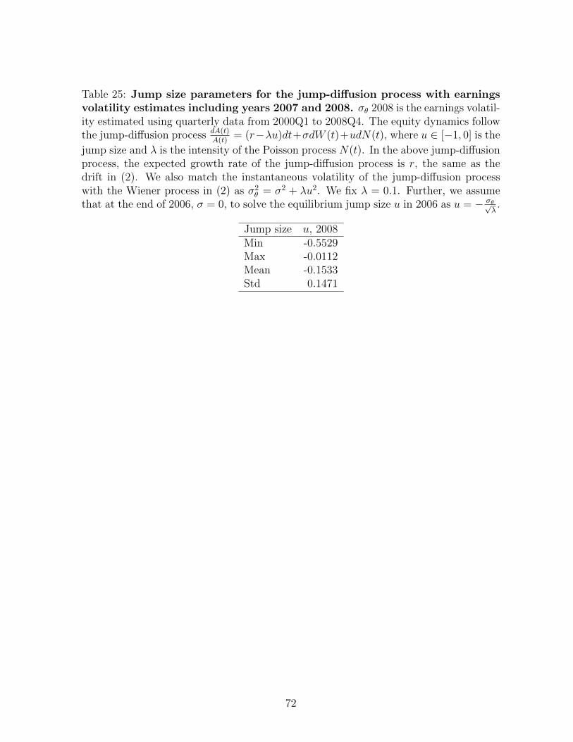
Table 25: Jump size parameters for the jump-diffusion process with earningsvolatility estimates including years 2007 and 2008. σθ 2008 is the earnings volatil-ity estimated using quarterly data from 2000Q1 to 2008Q4. The equity dynamics followthe jump-diffusion process dA(t)

A(t)= (r−λu)dt+σdW (t)+udN(t), where u ∈ [−1, 0] is the

jump size and λ is the intensity of the Poisson process N(t). In the above jump-diffusionprocess, the expected growth rate of the jump-diffusion process is r, the same as thedrift in (2). We also match the instantaneous volatility of the jump-diffusion processwith the Wiener process in (2) as σ2

θ = σ2 + λu2. We fix λ = 0.1. Further, we assumethat at the end of 2006, σ = 0, to solve the equilibrium jump size u in 2006 as u = − σθ√

λ.

Jump size u, 2008Min -0.5529Max -0.0112Mean -0.1533Std 0.1471

72

Table 26: Jump size increments for bonus caps and bonus deferrals with earnings volatility estimates includingyears 2007 and 2008. The bank-level bonus cap is the CEO’s annual salary in 2006 if the bonus interval is one year, thebonus cap is twice the CEO’s annual salary in 2006 if the bonus interval is two years, and the bonus cap is five times theCEO’s annual salary in 2006 if the bonus interval is five years. σ∗T,∞ is the estimated earnings volatility using the quarterlydata from 2000Q1 to 2008Q4. k is the cash bonus per net income in Panel A of Table 1. The average k during 2004-2006is used in this table. The equity dynamics follow the jump-diffusion process dA(t)

A(t)= (r − λu)dt + σdW (t) + udN(t), where

u ∈ [−1, 0] is the jump size and λ is the intensity of the Poisson process N(t). In the above jump-diffusion process, theexpected growth rate of the jump-diffusion process is r, the same as the drift in (2). We also match the instantaneousvolatility of the jump-diffusion process with the Wiener process in (2) as σ2

θ = σ2 + λu2. Similar to the optimality conditionin (11), the banker’s objective is to maximize πn,M(u∗T,∞+ ∆u)−F (∆u), where u∗T,∞ is the equilibrium jump size; see Table25. The optimal jump size is denoted as u∗n,M .

Case I: Bonus Case II: Bonus Case III: Bonus Case IV: Bonus Case V: Bonusinterval of 1 year interval of 2 years interval of 2 years interval of 5 years interval of 5 years

& bonus cap & no bonus cap & bonus cap & no bonus cap & bonus cap(u∗T,∞−u

∗T,S

u∗T,∞

) (u∗T,∞−u

∗T/2,∞

u∗T,∞

) (u∗T,∞−u

∗T/2,2S

u∗T,∞

) (u∗T,∞−u

∗T/5,∞

u∗T,∞

) (u∗T,∞−u

∗T/5,5S

u∗T,∞

)Linear Quadratic Linear Quadratic Linear Quadratic Linear Quadratic Linear Quadratic

Panel A: T cap 10 yrs.Min 0.00% 0.00% 0.00% 0.00% 0.00% 0.10% 0.00% 0.00% 0.00% 0.10%Max 0.00% 4.30% 0.00% 0.00% 0.00% 0.00% 0.00% 0.00% 0.00% 0.00%Mean 0.00% 0.06% 0.00% 0.00% 0.00% 0.00% 0.00% 0.00% 0.00% 0.00%Std 0.00% 0.49% 0.00% 0.00% 0.00% 0.01% 0.00% 0.00% 0.00% 0.01%Panel B: T cap 15 yrs.Min 0.00% 0.00% 0.00% 0.00% 0.00% 0.10% 0.00% 0.00% 0.00% 0.10%Max 0.00% 4.30% 0.00% 0.00% 0.00% 0.00% 0.00% 0.00% 0.00% 0.00%Mean 0.00% 0.06% 0.00% 0.00% 0.00% 0.00% 0.00% 0.00% 0.00% 0.00%Std 0.00% 0.49% 0.00% 0.00% 0.00% 0.01% 0.00% 0.00% 0.00% 0.02%

73