Bohmian Mechanics

Detlef Durr · Stefan Teufel

Bohmian Mechanics

The Physics and Mathematicsof Quantum Theory

123

ISBN 978-3-540-89343-1 e-ISBN 978-3-540-89344-8DOI 10.1007/978-3-540-89344-8Springer Dordrecht Heidelberg London New York

Library of Congress Control Number: 2009922149

c© Springer-Verlag Berlin Heidelberg 2009This work is subject to copyright. All rights are reserved, whether the whole or part of the material isconcerned, specifically the rights of translation, reprinting, reuse of illustrations, recitation, broadcasting,reproduction on microfilm or in any other way, and storage in data banks. Duplication of this publicationor parts thereof is permitted only under the provisions of the German Copyright Law of September 9,1965, in its current version, and permission for use must always be obtained from Springer. Violationsare liable to prosecution under the German Copyright Law.The use of general descriptive names, registered names, trademarks, etc. in this publication does notimply, even in the absence of a specific statement, that such names are exempt from the relevant protectivelaws and regulations and therefore free for general use.

Cover design: deblik, Berlin

Printed on acid-free paper

Springer is part of Springer Science+Business Media (www.springer.com)

Prof. Detlef DurrUniversitat MunchenFak. MathematikTheresienstr. 3980333 MunchenGermanydetlef.duerr@lmu.de

Prof. Stefan TeufelMathematisches InstitutAuf der Morgenstelle 1072076 TubingenGermanystefan.teufel@uni-tuebingen.de

Preface

This book is about Bohmian mechanics, a non-relativistic quantum theory basedon a particle ontology. As such it is a consistent theory of quantum phenomena, i.e.,none of the mysteries and paradoxes which plague the usual descriptions of quantummechanics arise. The most important message of this book is that quantum mechan-ics, as defined by its most general mathematical formalism, finds its explication inthe statistical analysis of Bohmian mechanics following Boltzmann’s ideas.

The book connects the physics with the abstract mathematical formalism andprepares all that is needed to achieve a commonsense understanding of the non-relativistic quantum world. Therefore this book may be of interest to both physicistsand mathematicians. The latter, who usually aim at unerring precision, are oftenput off by the mystical-sounding phrases surrounding the abstract mathematics ofquantum mechanics. In this book we aim at a precision which will also be acceptableto mathematicians.

Bohmian mechanics, named after its inventor David Bohm,1 is about the motionof particles. The positions of particles constitute the primitive variables, the primaryontology. For a quantum physicist the easiest way to grasp Bohmian mechanicsand to write down its defining equations is to apply the dictum: Whenever you sayparticle, mean it!

The key insight for analyzing Bohmian mechanics lies within the foundations ofstatistical physics. The reader will find it worth the trouble to work through Chap. 2on classical physics and Chap. 4 on chance, which are aimed at the understandingof the statistical analysis of a physical theory as it was developed by the great physi-cist Ludwig Boltzmann. Typicality is the ticket to get to the statistical import ofBohmian mechanics, which is succinctly captured by ρ = |ψ|2. The justification for

1 The equations were in fact already written down by the mathematical physicist Erwin Madelung,even before the famous physicist Louis de Broglie suggested the equations at the famous 1927Solvay conference. But these are unimportant historical details, which have no significance for theunderstanding of the theory. David Bohm was not aware of these early attempts, and moreoverhe presented the full implications of the theory for the quantum formalism. The theory is alsocalled the pilot wave theory or the de Broglie–Bohm theory, but Bohm himself called it the causalinterpretation of quantum mechanics.

v

vi Preface

this and the analysis of its consequences are two central points in the book. One ma-jor consequence is the emergence of the abstract mathematical structure of quantummechanics, observables as operators on Hilbert space, POVMS, and Heisenberg’suncertainty relation. All this and more follows from the theory of particles in mo-tion.

But this is not the only reason for the inclusion of some purely mathematicalchapters. Schrodinger’s cat story is world famous. A common argument to diminishthe measurement problem is that the quantum mechanical description of a cat in abox is so complicated, the mathematics so extraordinarily involved, that nobody hasdone that yet. But, so the argument continues, it could in principle be done, and ifall the mathematics is done properly and if one introduces all the observables withtheir domains of definitions in a proper manner, in short, if one does everything ina mathematically correct way, then there is no measurement problem. This answeralso appears in disguise as the claim that decoherence solves the measurement prob-lem. But this is false! It is precisely because one can in principle describe a cat ina box quantum mechanically that the problem is there and embarrassingly plain tosee. We have included all the mathematics required to ensure that no student of thesubject can be tricked into believing that everything in quantum physics would bealright if only the mathematics were done properly.

Bohmian mechanics has been around since 1952. It was promoted by John Bellin the second half of the last century. In particular, it was the manifestly nonlocalstructure of Bohmian mechanics that led Bell to his celebrated inequalities, whichallow us to check experimentally whether nature is local. Experiments have provedthat nature is nonlocal, just as Bohmian mechanics predicted. Nevertheless therewas once a time when physicists said that Bell’s inequalities proved that Bohmianmechanics was impossible. In fact, all kinds of criticisms have been raised againstBohmian mechanics. Since Bohmian mechanics is so simple and straightforward,only one criticism remains: there must be something wrong with Bohmian mechan-ics, otherwise it would be taught. And as a consequence, Bohmian mechanics is nottaught because there must be something wrong with it, otherwise it would be taught.We try in this book to show how Bohmian mechanics could be taught.

Any physicist who is ready to quantize everything under his pen should knowwhat quantization means in the simplest and established frame of non-relativisticphysics, and learn what conclusions should be drawn from that. The one conclusionwhich cannot be drawn is that nothing exists, or more precisely, that what existscannot be named within a mathematically consistent theory! For indeed it can! Thelesson here is that one should never give up ontology! If someone says: “I do notknow what it means to exist,” then that is fine. That person can view the theory ofBohmian mechanics as a precise and coherent mathematical theory, in which all thatneeds to be said is written in the equations, ready for analysis.

Our guideline for writing the book was the focus on the genesis of the ideas andconcepts, to be clear about what it is that we are talking about, and hence to pave theway for the hard technical work of learning how it is done. In short, we have triednot to leave out the letter ‘h’ (see the Melville quote on p. 4).

Preface vii

References

The references we give are neither complete nor balanced. Naturally the referencesreflect our point of view. They are nevertheless chosen in view of their basic charac-ter, sometimes containing many further references which the reader may follow upto achieve a more complete picture.

Acknowledgements

The present book is a translation and revision of the book Bohmsche Mechanik alsGrundlage der Quantenmechanik by one of the present authors (D.D.), publishedby Springer in 2001. The preface for this book read as follows: “In this book Iwrote down what I learned from my friends and colleagues Sheldon Goldstein andNino Zanghı. With their cooperation everything in this book would have been saidcorrectly – but only after an unforeseeably long time (extrapolating the times ittakes us to write a normal article). For that, I lack the patience (see the Epilogue)and I wanted to say things in my own style. Because of that, and only because ofthat, things may be said wrongly.” This paragraph is still relevant, of course, butwe feel the need to express our thanks to these truly great physicists and friendseven more emphatically. Without them this book would never have been written(but unfortunately with them perhaps also not). We have achieved our goal if theywould think of this as a good book. With them the (unwritten) book would havebeen excellent. Today we should like to add one more name: Roderich Tumulka, aformer student, now a distinguished researcher in the field of foundations who hassince helped us to gain further deep insights.

The long chapter on chance resulted from many discussions with Reinhard Langwhich clarified many issues. It was read and corrected several times by our stu-dent Christian Beck. Selected chapters were read, reread, and greatly improvedby our students and coworkers Dirk Deckert, Robert Grummt, Florian Hoffmann,Tilo Moser, Peter Pickl, Sarah Romer, and Georg Volkert. The whole text was care-fully read and critically discussed by the students of the reading class on Bohmianmechanics, and they are all thanked for their commitment. In particular, we wishto thank Dustin Lazarovici, Niklas Boers, and Florian Rieger for extensive andthoughtful corrections. We are especially grateful to Soren Petrat, who did a verydetailed and expert correction of the whole text.

The foundations of quantum mechanics are built on slippery grounds, and onedepends on friends and colleagues who encourage and support (with good criticism)this research, which is clearly not mainstream physics. Two important friends in thisundertaking are Giancarlo Ghirardi and Herbert Spohn. But there are more friendswe wish to acknowledge, who have, perhaps unknowingly, had a strong impact onthe writing of the book: Angelo Bassi, Gernot Bauer, Jurg Frohlich, Rodolfo Figari,Martin Kolb, Tim Maudlin, Sandro Teta, and Tim Storck.

We would also like to thank Wolf Beiglbock of Springer-Verlag, who encouragedand supported the English version of this book. Every author knows that a book can

viii Preface

be substantially improved by the editorial work done on it. We were extremely for-tunate that our editor was Angela Lahee at Springer, who astutely provided us withthe best copy-editor we could have wished for, namely Stephen Lyle, who brilliantlytransformed our Germanic English constructions into proper English without jeop-ardizing our attempt to incite the reader to active contemplation throughout. Weare very grateful to both Angela and Stephen for helping us with our endeavour topresent Bohmian mechanics as a respectable part of physics.

Landsberg and Tubingen, Detlef DurrOctober 2008 Stefan Teufel

Contents

1 Introduction . . . . . . . . . . . . . . . . . . . . . . . . . . . . . . . . . . . . . . . . . . . . . . . . . . . 11.1 Ontology: What There Is . . . . . . . . . . . . . . . . . . . . . . . . . . . . . . . . . . . . 1

1.1.1 Extracts . . . . . . . . . . . . . . . . . . . . . . . . . . . . . . . . . . . . . . . . . . . . 11.1.2 In Brief: The Problem of Quantum Mechanics . . . . . . . . . . . . 41.1.3 In Brief: Bohmian Mechanics . . . . . . . . . . . . . . . . . . . . . . . . . . 6

1.2 Determinism and Realism . . . . . . . . . . . . . . . . . . . . . . . . . . . . . . . . . . . 9References . . . . . . . . . . . . . . . . . . . . . . . . . . . . . . . . . . . . . . . . . . . . . . . . . . . . . 10

2 Classical Physics . . . . . . . . . . . . . . . . . . . . . . . . . . . . . . . . . . . . . . . . . . . . . . . 112.1 Newtonian Mechanics . . . . . . . . . . . . . . . . . . . . . . . . . . . . . . . . . . . . . . . 122.2 Hamiltonian Mechanics . . . . . . . . . . . . . . . . . . . . . . . . . . . . . . . . . . . . . 132.3 Hamilton–Jacobi Formulation . . . . . . . . . . . . . . . . . . . . . . . . . . . . . . . . 242.4 Fields and Particles: Electromagnetism . . . . . . . . . . . . . . . . . . . . . . . . 262.5 No fields, Only Particles: Electromagnetism . . . . . . . . . . . . . . . . . . . . 342.6 On the Symplectic Structure of the Phase Space . . . . . . . . . . . . . . . . . 38References . . . . . . . . . . . . . . . . . . . . . . . . . . . . . . . . . . . . . . . . . . . . . . . . . . . . . 42

3 Symmetry . . . . . . . . . . . . . . . . . . . . . . . . . . . . . . . . . . . . . . . . . . . . . . . . . . . . . 43

4 Chance . . . . . . . . . . . . . . . . . . . . . . . . . . . . . . . . . . . . . . . . . . . . . . . . . . . . . . . 494.1 Typicality . . . . . . . . . . . . . . . . . . . . . . . . . . . . . . . . . . . . . . . . . . . . . . . . . 51

4.1.1 Typical Behavior. The Law of Large Numbers . . . . . . . . . . . . 544.1.2 Statistical Hypothesis and Its Justification . . . . . . . . . . . . . . . . 634.1.3 Typicality in Subsystems:

Microcanonical and Canonical Ensembles . . . . . . . . . . . . . . . 664.2 Irreversibility . . . . . . . . . . . . . . . . . . . . . . . . . . . . . . . . . . . . . . . . . . . . . . 80

4.2.1 Typicality Within Atypicality . . . . . . . . . . . . . . . . . . . . . . . . . . 814.2.2 Our Atypical Universe . . . . . . . . . . . . . . . . . . . . . . . . . . . . . . . . 894.2.3 Ergodicity and Mixing . . . . . . . . . . . . . . . . . . . . . . . . . . . . . . . . 90

4.3 Probability Theory . . . . . . . . . . . . . . . . . . . . . . . . . . . . . . . . . . . . . . . . . 964.3.1 Lebesgue Measure and Coarse-Graining . . . . . . . . . . . . . . . . . 96

ix

x Contents

4.3.2 The Law of Large Numbers . . . . . . . . . . . . . . . . . . . . . . . . . . . 102References . . . . . . . . . . . . . . . . . . . . . . . . . . . . . . . . . . . . . . . . . . . . . . . . . . . . . 107

5 Brownian motion . . . . . . . . . . . . . . . . . . . . . . . . . . . . . . . . . . . . . . . . . . . . . . 1095.1 Einstein’s Argument . . . . . . . . . . . . . . . . . . . . . . . . . . . . . . . . . . . . . . . . 1105.2 On Smoluchowski’s Microscopic Derivation . . . . . . . . . . . . . . . . . . . . 1145.3 Path Integration . . . . . . . . . . . . . . . . . . . . . . . . . . . . . . . . . . . . . . . . . . . . 118References . . . . . . . . . . . . . . . . . . . . . . . . . . . . . . . . . . . . . . . . . . . . . . . . . . . . . 119

6 The Beginning of Quantum Theory . . . . . . . . . . . . . . . . . . . . . . . . . . . . . . 121References . . . . . . . . . . . . . . . . . . . . . . . . . . . . . . . . . . . . . . . . . . . . . . . . . . . . . 127

7 Schrodinger’s Equation . . . . . . . . . . . . . . . . . . . . . . . . . . . . . . . . . . . . . . . . . 1297.1 The Equation . . . . . . . . . . . . . . . . . . . . . . . . . . . . . . . . . . . . . . . . . . . . . . 1297.2 What Physics Must Not Be . . . . . . . . . . . . . . . . . . . . . . . . . . . . . . . . . . 1357.3 Interpretation, Incompleteness, and ρ = |ψ|2 . . . . . . . . . . . . . . . . . . . 139References . . . . . . . . . . . . . . . . . . . . . . . . . . . . . . . . . . . . . . . . . . . . . . . . . . . . . 143

8 Bohmian Mechanics . . . . . . . . . . . . . . . . . . . . . . . . . . . . . . . . . . . . . . . . . . . . 1458.1 Derivation of Bohmian Mechanics . . . . . . . . . . . . . . . . . . . . . . . . . . . . 1478.2 Bohmian Mechanics and Typicality . . . . . . . . . . . . . . . . . . . . . . . . . . . 1518.3 Electron Trajectories . . . . . . . . . . . . . . . . . . . . . . . . . . . . . . . . . . . . . . . . 1538.4 Spin . . . . . . . . . . . . . . . . . . . . . . . . . . . . . . . . . . . . . . . . . . . . . . . . . . . . . . 1588.5 A Topological View of Indistinguishable Particles . . . . . . . . . . . . . . . 166References . . . . . . . . . . . . . . . . . . . . . . . . . . . . . . . . . . . . . . . . . . . . . . . . . . . . . 171

9 The Macroscopic World . . . . . . . . . . . . . . . . . . . . . . . . . . . . . . . . . . . . . . . . 1739.1 Pointer Positions . . . . . . . . . . . . . . . . . . . . . . . . . . . . . . . . . . . . . . . . . . . 1739.2 Effective Collapse . . . . . . . . . . . . . . . . . . . . . . . . . . . . . . . . . . . . . . . . . . 1799.3 Centered Wave packets . . . . . . . . . . . . . . . . . . . . . . . . . . . . . . . . . . . . . . 1839.4 The Classical Limit of Bohmian Mechanics . . . . . . . . . . . . . . . . . . . . . 1869.5 Some Further Observations . . . . . . . . . . . . . . . . . . . . . . . . . . . . . . . . . . 191

9.5.1 Dirac Formalism, Density Matrix,Reduced Density Matrix, and Decoherence . . . . . . . . . . . . . . . 191

9.5.2 Poincare Recurrence . . . . . . . . . . . . . . . . . . . . . . . . . . . . . . . . . 198References . . . . . . . . . . . . . . . . . . . . . . . . . . . . . . . . . . . . . . . . . . . . . . . . . . . . . 200

10 Nonlocality . . . . . . . . . . . . . . . . . . . . . . . . . . . . . . . . . . . . . . . . . . . . . . . . . . . . 20110.1 Singlet State and Probabilities for Anti-Correlations . . . . . . . . . . . . . 20510.2 Faster Than Light Signals? . . . . . . . . . . . . . . . . . . . . . . . . . . . . . . . . . . . 208References . . . . . . . . . . . . . . . . . . . . . . . . . . . . . . . . . . . . . . . . . . . . . . . . . . . . . 209

11 The Wave Function and Quantum Equilibrium . . . . . . . . . . . . . . . . . . . . 21111.1 Measure of Typicality . . . . . . . . . . . . . . . . . . . . . . . . . . . . . . . . . . . . . . . 21111.2 Conditional Wave Function . . . . . . . . . . . . . . . . . . . . . . . . . . . . . . . . . . 21311.3 Effective Wave function . . . . . . . . . . . . . . . . . . . . . . . . . . . . . . . . . . . . . 216

Contents xi

11.4 Typical Empirical Distributions . . . . . . . . . . . . . . . . . . . . . . . . . . . . . . . 21811.5 Misunderstandings . . . . . . . . . . . . . . . . . . . . . . . . . . . . . . . . . . . . . . . . . 22311.6 Quantum Nonequilibrium . . . . . . . . . . . . . . . . . . . . . . . . . . . . . . . . . . . . 224References . . . . . . . . . . . . . . . . . . . . . . . . . . . . . . . . . . . . . . . . . . . . . . . . . . . . . 225

12 From Physics to Mathematics . . . . . . . . . . . . . . . . . . . . . . . . . . . . . . . . . . . 22712.1 Observables. An Unhelpful Notion . . . . . . . . . . . . . . . . . . . . . . . . . . . . 22712.2 Who Is Afraid of PVMs and POVMs? . . . . . . . . . . . . . . . . . . . . . . . . . 233

12.2.1 The Theory Decides What Is Measurable . . . . . . . . . . . . . . . . 24112.2.2 Joint Probabilities . . . . . . . . . . . . . . . . . . . . . . . . . . . . . . . . . . . . 24212.2.3 Naive Realism about Operators . . . . . . . . . . . . . . . . . . . . . . . . 244

12.3 Schrodinger’s Equation Revisited . . . . . . . . . . . . . . . . . . . . . . . . . . . . . 24512.4 What Comes Next? . . . . . . . . . . . . . . . . . . . . . . . . . . . . . . . . . . . . . . . . . 248References . . . . . . . . . . . . . . . . . . . . . . . . . . . . . . . . . . . . . . . . . . . . . . . . . . . . . 249

13 Hilbert Space . . . . . . . . . . . . . . . . . . . . . . . . . . . . . . . . . . . . . . . . . . . . . . . . . . 25113.1 The Hilbert Space L2 . . . . . . . . . . . . . . . . . . . . . . . . . . . . . . . . . . . . . . . 253

13.1.1 The Coordinate Space �2 . . . . . . . . . . . . . . . . . . . . . . . . . . . . . . 25513.1.2 Fourier Transformation on L2 . . . . . . . . . . . . . . . . . . . . . . . . . . 258

13.2 Bilinear Forms and Bounded Linear Operators . . . . . . . . . . . . . . . . . . 26813.3 Tensor Product Spaces . . . . . . . . . . . . . . . . . . . . . . . . . . . . . . . . . . . . . . 271References . . . . . . . . . . . . . . . . . . . . . . . . . . . . . . . . . . . . . . . . . . . . . . . . . . . . . 278

14 The Schrodinger Operator . . . . . . . . . . . . . . . . . . . . . . . . . . . . . . . . . . . . . . 27914.1 Unitary Groups and Their Generators . . . . . . . . . . . . . . . . . . . . . . . . . . 27914.2 Self-Adjoint Operators . . . . . . . . . . . . . . . . . . . . . . . . . . . . . . . . . . . . . . 28414.3 The Atomistic Schrodinger Operator . . . . . . . . . . . . . . . . . . . . . . . . . . 294References . . . . . . . . . . . . . . . . . . . . . . . . . . . . . . . . . . . . . . . . . . . . . . . . . . . . . 298

15 Measures and Operators . . . . . . . . . . . . . . . . . . . . . . . . . . . . . . . . . . . . . . . . 29915.1 Examples of PVMs and Their Operators . . . . . . . . . . . . . . . . . . . . . . . 303

15.1.1 Heisenberg Operators . . . . . . . . . . . . . . . . . . . . . . . . . . . . . . . . . 30515.1.2 Asymptotic Velocity and the Momentum Operator . . . . . . . . 306

15.2 The Spectral Theorem . . . . . . . . . . . . . . . . . . . . . . . . . . . . . . . . . . . . . . . 31115.2.1 The Dirac Formalism . . . . . . . . . . . . . . . . . . . . . . . . . . . . . . . . . 31115.2.2 Mathematics of the Spectral Theorem . . . . . . . . . . . . . . . . . . . 31315.2.3 Spectral Representations . . . . . . . . . . . . . . . . . . . . . . . . . . . . . . 32215.2.4 Unbounded Operators . . . . . . . . . . . . . . . . . . . . . . . . . . . . . . . . 32415.2.5 Unitary Groups . . . . . . . . . . . . . . . . . . . . . . . . . . . . . . . . . . . . . . 33215.2.6 H0 =−Δ/2 . . . . . . . . . . . . . . . . . . . . . . . . . . . . . . . . . . . . . . . . . 33315.2.7 The Spectrum . . . . . . . . . . . . . . . . . . . . . . . . . . . . . . . . . . . . . . . 341

References . . . . . . . . . . . . . . . . . . . . . . . . . . . . . . . . . . . . . . . . . . . . . . . . . . . . . 344

xii Contents

16 Bohmian Mechanics on Scattering Theory . . . . . . . . . . . . . . . . . . . . . . . . 34516.1 Exit Statistics . . . . . . . . . . . . . . . . . . . . . . . . . . . . . . . . . . . . . . . . . . . . . . 34616.2 Asymptotic Exits . . . . . . . . . . . . . . . . . . . . . . . . . . . . . . . . . . . . . . . . . . . 35316.3 Scattering Theory and Exit Distribution . . . . . . . . . . . . . . . . . . . . . . . . 35616.4 More on Abstract Scattering Theory . . . . . . . . . . . . . . . . . . . . . . . . . . . 35816.5 Generalized Eigenfunctions . . . . . . . . . . . . . . . . . . . . . . . . . . . . . . . . . . 36116.6 Towards the Scattering Cross-Section . . . . . . . . . . . . . . . . . . . . . . . . . . 36816.7 The Scattering Cross-Section . . . . . . . . . . . . . . . . . . . . . . . . . . . . . . . . . 369

16.7.1 Born’s Formula . . . . . . . . . . . . . . . . . . . . . . . . . . . . . . . . . . . . . . 37016.7.2 Time-Dependent Scattering . . . . . . . . . . . . . . . . . . . . . . . . . . . . 372

References . . . . . . . . . . . . . . . . . . . . . . . . . . . . . . . . . . . . . . . . . . . . . . . . . . . . . 378

17 Epilogue . . . . . . . . . . . . . . . . . . . . . . . . . . . . . . . . . . . . . . . . . . . . . . . . . . . . . . 379References . . . . . . . . . . . . . . . . . . . . . . . . . . . . . . . . . . . . . . . . . . . . . . . . . . . . . 380

Bibliography . . . . . . . . . . . . . . . . . . . . . . . . . . . . . . . . . . . . . . . . . . . . . . . . . . . . . . . 381

Index . . . . . . . . . . . . . . . . . . . . . . . . . . . . . . . . . . . . . . . . . . . . . . . . . . . . . . . . . . . . . 387

Chapter 1Introduction

1.1 Ontology: What There Is

1.1.1 Extracts

Sometimes quantization is seen as the procedure that puts hats on classical observ-ables to turn them into quantum observables.

Lewis Carroll on Hatters and Cats

Lewis Carroll (alias Charles Lutwidge Dodgson 1832–1898) was professor of math-ematics at Oxford (where Schrodinger wrote his famous cat article):

The Cat only grinned when it saw Alice. It looked good-natured, she thought: still it hadVERY long claws and a great many teeth, so she felt that it ought to be treated with respect.“Cheshire Puss,” she began, rather timidly, as she did not at all know whether it would likethe name: however, it only grinned a little wider. “Come, it’s pleased so far,” thought Alice,and she went on. “Would you tell me, please, which way I ought to go from here?” “Thatdepends a good deal on where you want to get to,” said the Cat. “I don’t much care where–” said Alice. “Then it doesn’t matter which way you go,” said the Cat. “– so long as I getSOMEWHERE,” Alice added as an explanation. “Oh, you’re sure to do that,” said the Cat,“if you only walk long enough.” Alice felt that this could not be denied, so she tried anotherquestion. “What sort of people live about here?” “In THAT direction,” the Cat said, wavingits right paw round, “lives a Hatter: and in THAT direction,” waving the other paw, “lives aMarch Hare. Visit either you like: they’re both mad.” “But I don’t want to go among madpeople,” Alice remarked. “Oh, you can’t help that,” said the Cat: “we’re all mad here. I’mmad. You’re mad.” “How do you know I’m mad?” said Alice. “You must be,” said the Cat,“or you wouldn’t have come here.” Alice didn’t think that proved it at all; however, shewent on “And how do you know that you’re mad?” “To begin with,” said the Cat, “a dog’snot mad. You grant that?” “I suppose so,” said Alice. “Well, then,” the Cat went on, “yousee, a dog growls when it’s angry, and wags its tail when it’s pleased. Now I growl whenI’m pleased, and wag my tail when I’m angry. Therefore I’m mad.” “I call it purring, notgrowling,” said Alice. “Call it what you like,” said the Cat. “Do you play croquet with the

D. Durr, S. Teufel, Bohmian Mechanics, DOI 10.1007/978-3-540-89344-8 1, 1c© Springer-Verlag Berlin Heidelberg 2009

2 1 Introduction

Queen today?” “I should like it very much,” said Alice, “but I haven’t been invited yet.”“You’ll see me there,” said the Cat, and vanished.

Alice was not much surprised at this, she was getting so used to queer things happening.While she was looking at the place where it had been, it suddenly appeared again.

Alice’s Adventures in Wonderland (1865) [1].

Parmenides on What There Is

The Greek philosopher Parmenides of Elea wrote as follows in the sixth centuryBC:

Come now, I will tell thee – and do thou hearken to my saying and carry it away – theonly two ways of search that can be thought of. The first, namely, that It is, and that it isimpossible for it not to be, is the way of belief, for truth is its companion. The other, namely,that It is not, and that it must needs not be, – that, I tell thee, is a path that none can learnof at all. For thou canst not know what is not – that is impossible – nor utter it; for it is thesame thing that can be thought and that can be.

It needs must be that what can be spoken and thought is; for it is possible for it to be, andit is not possible for what is nothing to be. This is what I bid thee ponder. I hold thee backfrom this first way of inquiry, and from this other also, upon which mortals knowing naughtwander two-faced; for helplessness guides the wandering thought in their breasts, so thatthey are borne along stupefied like men deaf and blind. Undiscerning crowds, who hold thatit is and is not the same and not the same, and all things travel in opposite directions!

For this shall never be proved, that the things that are not are; and do thou restrain thythought from this way of inquiry.

The Way of Truth [2].

It is sometimes said that, in quantum mechanics, the observer calls things into beingby the act of observation.

Schrodinger on Quantum Mechanics

Erwin Schrodinger wrote in 1935:

One can even set up quite ridiculous cases. A cat is penned up in a steel chamber, alongwith the following device (which must be secured against direct interference by the cat):in a Geiger counter there is a tiny bit of radioactive substance, so small, that perhaps inthe course of the hour one of the atoms decays, but also, with equal probability, perhapsnone; if it happens, the counter tube discharges and through a relay releases a hammerwhich shatters a small flask of hydrocyanic acid. If one has left this entire system to itselffor an hour, one would say that the cat still lives if meanwhile no atom has decayed. Thepsi-function of the entire system would express this by having in it the living and dead cat(pardon the expression) mixed or smeared out in equal parts.

It is typical of these cases that an indeterminacy originally restricted to the atomic domainbecomes transformed into macroscopic indeterminacy, which can then be resolved by directobservation. That prevents us from so naively accepting as valid a “blurred model” for

1.1 Ontology: What There Is 3

representing reality. In itself it would not embody anything unclear or contradictory. Thereis a difference between a shaky or out-of-focus photograph and a snapshot of clouds andfog banks.

Die gegenwartige Situation in der Quantenmechanik [3].Translated by J.D. Trimmer in [4].

The difference between a shaky photograph and a snapshot of clouds and fog banksis the difference between Bohmian mechanics and quantum mechanics. In itself a“blurred model” representing reality would not embody anything unclear, whereasresolving the indeterminacy by direct observation does. As if observation were notpart of physics.

Feynman on Quantum Mechanics

Feynman said the following:

Does this mean that my observations become real only when I observe an observer observ-ing something as it happens? This is a horrible viewpoint. Do you seriously entertain thethought that without observer there is no reality? Which observer? Any observer? Is a fly anobserver? Is a star an observer? Was there no reality before 109 B.C. before life began? Orare you the observer? Then there is no reality to the world after you are dead? I know a num-ber of otherwise respectable physicists who have bought life insurance. By what philosophywill the universe without man be understood?

Lecture Notes on Gravitation [5].

Bell on Quantum Mechanics

According to John S. Bell:

It would seem that the theory is exclusively concerned about “results of measurement”,and has nothing to say about anything else. What exactly qualifies some physical systemsto play the role of “measurer”? Was the wavefunction of the world waiting to jump forthousands of years until a single-celled living creature appeared? Or did it have to wait alittle longer, for some better qualified system [. . . ] with a Ph.D.? If the theory is to apply toanything but highly idealized laboratory operations, are we not obliged to admit that moreor less “measurement-like” processes are going on more or less all the time, more or lesseverywhere? Do we not have jumping then all the time?

Against “measurement” [6].

Einstein on Measurements

But it is in principle quite false to base a theory solely on observable quantities. Since, infact, it is the other way around. It is the theory that decides what we can observe.

Albert Einstein, cited by Werner Heisenberg1 in [7].

1 Quoted from Die Quantenmechanik und ein Gesprach mit Einstein. Translation by Detlef Durr.

4 1 Introduction

Melville on Omissions

While you take in hand to school others, and to teach them by what name a whale-fish isto be called in our tongue leaving out, through ignorance, the letter H, which almost alonemaketh the signification of the word, you deliver that which is not true.

Melville (1851), Moby Dick; or, The Whale, Etymology [8].

1.1.2 In Brief: The Problem of Quantum Mechanics

Schrodinger remarks in his laconic way that there is a difference between a shakyor out-of-focus photograph and a snapshot of clouds and fog banks.

The first problem with quantum mechanics is that it is not about what there is. Itis said to be about the microscopic world of atoms, but it does not spell out whichphysical quantities in the theory describe the microscopic world. Which variablesspecify what is microscopically there? Quantum mechanics is about the wave func-tion. The wave function lives on configuration space, which is the coordinate spaceof all the particles participating in the physical process of interest. That the wavefunction lives on configuration space has been called by Schrodinger entanglementof the wave function. The wave function obeys a linear equation – the Schrodingerequation. The linearity of the Schrodinger equation prevents the wave function fromrepresenting reality.2 We shall see that in a moment. The second problem of quan-tum mechanics is that the first problem provokes many rich answers, which to theuntrained ear appear to be of philosophical nature, but which leave the problemunanswered: What is it that quantum mechanics is about?

It is said for example that the virtue of quantum mechanics is that it is only aboutwhat can be measured. Moreover, that what can be measured is defined throughthe measurement. Without measurement there is nothing there. But a measurementbelongs to the macroscopic world (which undeniably exists), and its macroscopicconstituents like the measurement apparatus are made out of atoms, which quantummechanics is supposed to describe, so this entails that the apparatus itself is to be de-scribed quantum mechanically. This circularity lies at the basis of the measurementproblem of quantum mechanics, which is often phrased as showing incompletenessof quantum mechanics. Some things, namely the objects the theory is about, havebeen left out of the description, or the description – the Schrodinger equation – isnot right. Mathematically the measurement problem may be presented as follows.Suppose a system is described by linear combinations of wave functions ϕ1 and ϕ2.Suppose there exists a piece of apparatus which, when brought into interaction withthe system, measures whether the system has wave function ϕ1 or ϕ2. Measuring

2 Even if the equation were nonlinear, as is the case in reduction models, the wave function livingon configuration space could not by itself represent reality in physical space. There must still besome “beable” (related to the wave function) in the sense of Bell [9] representing physical reality.But we ignore this fine point here.

1.1 Ontology: What There Is 5

means that, next to the 0 pointer position, the apparatus has two pointer positions 1and 2 “described” by wave functionsΨ0,Ψ1, andΨ2, for which

ϕiΨ0Schrodinger evolution−→ ϕiΨi , i = 1,2 . (1.1)

When we say that the pointer positions are “described” by wave functions, we meanthat in a loose sense. The wave function has a support in configuration space whichcorresponds classically to a set of coordinates of particles which would form apointer.

The Schrodinger equation is linear, so for the superposition, (1.1) yields

ϕ = c1ϕ1 + c2ϕ2 , c1,c2 ∈ C , |c1|2 + |c2|2 = 1 ,

ϕΨ0 = (c1ϕ1 + c2ϕ2)Ψ0Schrodinger evolution−→ c1ϕ1Ψ1 + c2ϕ2Ψ2 . (1.2)

The outcome on the right does not concur with experience. It shows rather a “macro-scopic indeterminacy”. In the words of Schrodinger, observation then resolves thismacroscopic indeterminacy, since one only observes either 1 (with probability |c1|2)or 2 (with probability |c2|2), i.e., observation resolves the blurred description of re-ality into one where the wave function is either ϕ1Ψ1 or ϕ2Ψ2. In Schrodinger’s catthought experiment ϕ1,2 are the wave functions of the non-decayed and decayedatom andΨ0,1 are the wave functions of the live cat andΨ2 is the wave function ofthe dead cat. Schrodinger says that this is unacceptable. But why? Is the apparatusnot supposed to be the observer? What qualifies us better than the apparatus, whichwe designed in such a way that it gives a definite outcome and not a blurred one?

The question is: what in the theory describes the actual facts? Either those vari-ables which describe the actual state of affairs have been left out of the description(Bohmian mechanics makes amends for that) or the Schrodinger equation whichyields the unrealistic result (1.2) from (1.1) is false. (GRW theories, or more gen-erally, dynamical reduction models, follow the latter way of describing nature. Thewave function collapses by virtue of the dynamical law [10].)

The evolution in (1.2) is an instance of the so-called decoherence. The apparatusdecoheres the superposition c1ϕ1 +c2ϕ2 of the system wave function. Decoherencemeans that it is in a practical sense impossible to get the two wave packets ϕ1Ψ1 andϕ2Ψ2 superposed in c1ϕ1Ψ1 + c2ϕ2Ψ2 to interfere. It is sometimes said that, takingdecoherence into account, there would not be any measurement problem. Deco-herence is this practical impossibility, which Bell referred to as fapp-impossibility(where fapp means for all practical purposes), of the interference of the pointerwave functions. It is often dressed up, for better looks, in terms of density matrices.In Dirac’s notation, the density matrix is

ρG = |c1|2|ϕ1〉|Ψ1〉〈Ψ1|〈ϕ1|+ |c2|2|ϕ2〉|Ψ2〉〈Ψ2|〈ϕ2| .

6 1 Introduction

This can be interpreted as describing a statistical mixture of the two states |ϕ1〉|Ψ1〉and |ϕ2〉|Ψ2〉, and one can say that in a fapp sense the pure state given by the right-hand side of (1.2), namely

ρ = |c1ϕ1Ψ1 + c2ϕ2Ψ2〉〈c1Ψ1ϕ1 + c2Ψ2ϕ2| ,

is close to ρG. They are fapp-close because the off-diagonal element

c1c∗2|Ψ1ϕ1〉〈Ψ2ϕ2|

where the asterisk denotes complex conjugation, would only be observable if thewave parts could be brought into interference, which is fapp-impossible. The argu-ment then concludes that the meaning of the right-hand side of (1.2) is fapp-closeto the meaning of the statistical mixture. To emphasise the fact that such argumentsmiss the point of the exercise, Schrodinger made his remark that there is a differ-ence between a shaky or out-of-focus photograph and a snapshot of clouds and fogbanks.

To sum up then, decoherence does not create the facts of our world, but ratherproduces a sequence of fapp-redundancies, which physically increase or stabilizedecoherence. So the cat decoheres the atom, the observer decoheres the cat thatdecoheres the atom, the environment of the observer decoheres the observer thatdecoheres the cat that decoheres the atom and so on. In short, what needs to bedescribed by the physical theory is the behavior of real objects, located in physicalspace, which account for the facts.

1.1.3 In Brief: Bohmian Mechanics

Bohmian mechanics is about point particles in motion. The theory was inventedin 1952 by David Bohm (1917–1992) [11] (there is a bit more on the history inChap. 7). In a Bohmian universe everything is made out of particles. Their motionis guided by the wave function. That is why the wave function is there. That is itsrole. The physical theory is formulated with the variables qi ∈ R

3, i = 1,2, . . . ,N,the positions of the N particles which make up the system, and the wave func-tion ψ(q1, . . . ,qN) on the configuration space of the system. If the wave functionconsists of two parts which have disjoint supports in configuration space, then thesystem configuration is in one or the other support. In the measurement example,the pointer configuration is either in the support suppΨ1 ofΨ1 (pointing out 1) or inthe support suppΨ2 ofΨ2 (pointing out 2).

Bohmian mechanics happens to be deterministic. A substantial success of Bohmianmechanics is the explanation of quantum randomness or Born’s statistical law, onthe basis of Boltzmann’s principles of statistical mechanics, i.e., Born’s law is notan axiom but a theorem in Bohmian mechanics. Born’s statistical law concerningρ = |ψ|2 says that, if the wave function is ψ , the particle configuration is |ψ|2-distributed. Applying this to (1.2) implies that the result i comes with probability

1.1 Ontology: What There Is 7

|ci|2. Suppose the enlarged system composed of system plus apparatus is describedby the configuration coordinates q = (x,y), where x ∈ R

m is the system configura-tion and y ∈R

n the pointer configuration. We compute the probability for the result1 by Born’s law. This means we compute the probability that the true (or actual)pointer configuration Y lies in the support suppΨ1. In the following computation,we assume that the wave functions are all normalized to unity. Then

P(pointer on1) =∫

suppΨ1

|c1ϕ1Ψ1 + c2ϕ2Ψ2|2dmxdny (1.3a)

= |c1|2∫

suppΨ1

|ϕ1Ψ1|2dmxdny+ |c2|2∫

suppΨ1

|ϕ2Ψ2|2dmxdny

+2ℜ[

c∗1c2

∫suppΨ1

(ϕ1Ψ1)∗ϕ2Ψ2dmxdny

](1.3b)

= |c1|2∫|ϕ1Ψ1|2dmxdny = |c1|2 , (1.3c)

where ℜ in (1.3b) denotes the real part of a complex quantity. The terms involvingΨ2 yield zero because of the disjointness3 of the supports of the pointer wave func-tionsΨ1,Ψ2. This result holds fapp-forever, since it is fapp-impossible for the wavefunction partsΨ1 andΨ2 to interfere in the future, especially when the results havebeen written down or recorded in any way – the ever growing decoherence.

Suppose one removes the positions of the particles from the theory, as for ex-ample Heisenberg, Bohr, and von Neumann did. Then to be able to conclude fromthe fapp-impossibility of interference that only one of the wave functions remains,one needs to add an “observer” who by the act of observation collapses the wavefunction with probability |ci|2 to the Ψi part, thereby “creating” the result i. Onceagain, we may ask what qualifies an observer as better than a piece of apparatusor a cat. Debate of this kind has been going on since the works of Heisenberg andSchrodinger in 1926. The debate, apart from producing all kinds of philosophicaltreatises, revolves around the collapse of the wave function. But when does the col-lapse happen and who is entitled to collapse the wave function? Does the collapsehappen at all? It is, to put it mildly, a bit puzzling that such an obvious shortcomingof the theory has led to such a confused and unfocussed debate. Indeed, it has shownphysics in a bad light. In Bohmian mechanics, the collapse does not happen at all,although there is a fapp-collapse, which one may introduce when one analyzes thetheory. In collapse theories (like GRW), the collapse does in fact happen. Bohmianmechanics and collapse theories differ in that way. They make different predictionsfor macroscopic interference experiments, which may, however, be very difficult toperform, if not fapp-impossible.

We did not say how the particles are guided by the wave function. One getsthat by simply taking language seriously. Whenever you say “particle” in quantummechanics, mean it! That is Bohmian mechanics. All problems evaporate on the

3 The wave functions will in reality overlap, but the overlap is negligible. Therefore the wavefunctions are well approximated by wave functions with disjoint supports.

8 1 Introduction

spot. In a nutshell, the quantity |ψt |2, with ψt a solution of Schrodinger’s equation,satisfies a continuity equation, the so-called quantum flux equation. The particles inBohmian mechanics move along the flow lines of the quantum flux. In other wordsthe quantum flux equation is the continuity equation for transport of probabilityalong the Bohmian trajectories. Still not satisfied? Is that too cheap? Why the wavefunction? Why |ψt |2? We shall address all these questions and more in the chaptersto follow.

Bohmian mechanics is defined by two equations: one is the Schrodinger equationfor the guiding field ψt and one is the equation for the positions of the particles. Thelatter equation reads

Q = μℑ∇ψt(Q)ψt(Q)

, (1.4)

where ℑ denotes the imaginary part, and μ is an appropriate dimension factor. Thequantum formalism in its most general form, including all rules and axioms, fol-lows from this by analysis of the theory. In particular, Heisenberg’s uncertaintyrelation for position and momentum, from which it is often concluded that particletrajectories are in conflict with quantum mechanics, follows directly from Bohmianmechanics.

Bohmian mechanics is nonlocal in the sense of Bell’s inequalities and therefore,according to the experimental tests of Bell’s inequalities, concurs with the basicrequirements that any correct theory of nature must fulfill.

A Red Herring: The Double Slit Experiment

This is a quantum mechanical experiment which is often cited as conflicting withthe idea that there can be particles with trajectories. One sends a particle (i.e., a wavepacket ψ) through a double slit. Behind the slit at some distance is a photographicplate. When the particle arrives at the plate it leaves a black spot at its place of ar-rival. Nothing yet speaks against the idea that the particle moves on a trajectory. Butnow repeat the experiment. The next particle marks a different spot of the photo-graphic plate. Repeating this a great many times the spots begin to show a pattern.They trace out the points of constructive interference of the wave packet ψ which,when passing the two slits, shows the typical Huygens interference of two sphericalwaves emerging from each slit. Suppose the wave packet reaches the photographicplate after a time T . Then the spots show the |ψ(T )|2 distribution,4 in the sense thatthis is their empirical distribution. Analyzing this using Bohmian mechanics, i.e.,analyzing Schrodinger’s equation and the guiding equation (1.4), one immediatelyunderstands why the experiment produces the result it does. It is clear that in eachrun the particle goes either through the upper or through the lower slit. The wavefunction goes through both slits and forms after the slits a wave function with an

4 In fact, it is the quantum flux across the surface of the photographic plate, integrated over time(see Chap. 16).

1.2 Determinism and Realism 9

interference pattern. Finally the repetition of the experiment produces an ensemblewhich checks Born’s statistical law for that wave function. That is the straightfor-ward physical explanation.

So where is the argument which reveals a conflict with the notion of particletrajectories? Here it is:

Close slit 1 and open slit 2. (1.5a)

The particle goes through slit 2. (1.5b)

It arrives at x on the plate with probability |ψ2(x)|2, (1.5c)

where ψ2 is the wave function which passed through slit 2. Next

close slit 2 and open slit 1. (1.6a)

The particle goes through slit 1. (1.6b)

It arrives at x on the plate with probability |ψ1(x)|2, (1.6c)

where ψ1 is the wave function which passed through slit 1. Now open both slits.

Both slits are open. (1.7a)

The particle goes through slit 1 or slit 2. (1.7b)

It arrives at x with probability |ψ1(x)+ψ2(x)|2 . (1.7c)

Now observe that in general

|ψ1(x)+ψ2(x)|2 = |ψ1(x)|2 + |ψ2(x)|2 +2ℜψ∗1 (x)ψ2(x) �= |ψ1(x)|2 + |ψ2(x)|2 .

The �= comes from interference of the wave packetsψ1,ψ2 which passed through slit1 and slit 2. The argument now proceeds in the following way. Situations (1.5b) and(1.6b) are the exclusive alternatives entering (1.7b), so the probabilities (1.5c) and(1.6c) must add up. But they do not. So is logic false? Is the particle idea nonsense?No, the argument is a red herring, since (1.5a), (1.6a), and (1.7a) are physicallydistinct.

1.2 Determinism and Realism

It is often said that the aim of Bohmian mechanics is to restore determinism inthe quantum world. That is false. Determinism has nothing to do with ontology.What is “out there” could just as well be governed by stochastic laws, as is thecase in GRW or dynamical reduction models with, e.g., flash ontology [12, 13].A realistic quantum theory is a quantum theory which spells out what it is about.Bohmian mechanics is a realistic quantum theory. It happens to be deterministic,which is fine, but not an ontological necessity. The merit of Bohmian mechanicsis not determinism, but the refutation of all claims that quantum mechanics cannot

10 1 Introduction

be reconciled with a realistic description of reality. In physics, one needs to knowwhat is going on. Bohmian mechanics tells us what is going on and it does so in themost straightforward way imaginable. It is therefore the fundamental description ofGalilean physics.

The following passage taken from a letter from Pauli to Born, concerning Ein-stein’s view on determinism, is in many ways reminiscent of the present situation inBohmian mechanics:

Einstein gave me your manuscript to read; he was not at all annoyed with you, but onlysaid that you were a person who will not listen. This agrees with the impression I haveformed myself insofar as I was unable to recognise Einstein whenever you talked abouthim in either your letter or your manuscript. It seemed to me as if you had erected somedummy Einstein for yourself, which you then knocked down with great pomp. In particu-lar, Einstein does not consider the concept of “determinism” to be as fundamental as it isfrequently held to be (as he told me emphatically many times), and he denied energeticallythat he had ever put up a postulate such as (your letter, para. 3): “the sequence of such con-ditions must also be objective and real, that is, automatic, machine-like, deterministic.” Inthe same way, he disputes that he uses as a criterion for the admissibility of a theory thequestion: “Is it rigorously deterministic?” Einstein’s point of departure is “realistic” ratherthan “deterministic”.

Wolfgang Pauli, in [14], p. 221.

References

1. L. Carroll: The Complete, Fully Illustrated Works (Gramercy Books, New York, 1995)2. J. Burnet: Early Greek Philosophy (A. and C. Black, London and Edinburgh, 1930)3. E. Schrodinger: Naturwissenschaften 23, 807 (1935)4. J.A. Wheeler, W.H. Zurek (eds.): Quantum Theory and Measurement. Princeton Series in

Physics (Princeton University Press, Princeton, NJ, 1983)5. R.P. Feynman, F.B. Morinigo, W.G. Wagner: Feynman Lectures on Gravitation (Addison-

Wesley Publishing Company, 1959). Edited by Brian Hatfield6. M. Bell, K. Gottfried and M. Veltman (eds.): John S. Bell on the Foundations of Quantum

Mechanics (World Scientific Publishing Co. Inc., River Edge, NJ, 2001)7. W. Heisenberg: Quantentheorie und Philosophie, Universal-Bibliothek [Universal Library],

Vol. 9948 (Reclam-Verlag, Stuttgart, 1987). Vorlesungen und Aufsatze. [Lectures and essays],With an afterword by Jurgen Busche

8. H. Melville: Moby Dick; or, The Whale (William Benton, Encyclopaedia Britanica, Inc.,1952). Greatest Books of the Western World

9. J.S. Bell: Speakable and Unspeakable in Quantum Mechanics (Cambridge University Press,Cambridge, 1987)

10. A. Bassi, G. Ghirardi: Phys. Rep. 379 (5–6), 257 (2003)11. D. Bohm: Phys. Rev. 85, 166 (1952)12. J.S. Bell: Beables for quantum fields. In: Speakable and Unspeakable in Quantum Mechanics

(Cambridge University Press, 1987)13. R. Tumulka: J. Stat. Phys. 125 (4), 825 (2006)14. I. Born: The Born–Einstein Letters (Walker and Company, New York, 1971)

Chapter 2Classical Physics

What is classical physics? In fact it has become the name for non-quantum physics.This begs the question: What is quantum physics in contrast to classical physics?One readily finds the statement that in classical physics the world is described byclassical notions, like particles moving around in space, while in modern physics,i.e., quantum mechanics, the classical notions are no longer adequate, so there isno longer such a “naive” description of what is going on. In a more sophisticatedversion, quantum mechanics is physics in which the position and momentum of aparticle are operators. But such a statement as it stands is meaningless. One alsoreads that the difference between quantum physics and classical physics is that theformer has a smallest quantum of action, viz., Planck’s constant h, and that classicalphysics applies whenever the action is large compared to h, and in many circum-stances, this is a true statement.

But our own viewpoint is better expressed as follows. Classical physics is thedescription of the world when the interference effects of the Schrodinger wave,evolving according to Schrodinger’s equation, can be neglected. This is the casefor a tremendously wide range of scales from microscopic gases to stellar matter.In particular it includes the scale of direct human perception, and this explains whyclassical physics was found before quantum mechanics. Still, the viewpoint just ex-pressed should seem puzzling. For how can classical motion of particles emergefrom a wave equation like the Schrodinger equation? This is something we shallexplain. It is easy to understand, once one writes down the equations of motion ofBohmian mechanics. But first let us discuss the theory which governs the behaviorof matter across the enormous range of classical physics, namely, Newtonian me-chanics. In a letter to Hooke, Newton wrote: “If I have seen further it is by standingon the shoulders of giants.”

D. Durr, S. Teufel, Bohmian Mechanics, DOI 10.1007/978-3-540-89344-8 2, 11c© Springer-Verlag Berlin Heidelberg 2009

12 2 Classical Physics

2.1 Newtonian Mechanics

Newtonian mechanics is about point particles. What is a point particle? It is “stuff”or “matter” that occupies a point in space called its position, described mathemati-cally by q ∈ R

3. The theory describes the motion of point particles in space. Math-ematically, an N-particle system is described by the positions of the N particles:

q1, . . . ,qN , qi ∈ R3 ,

which change with time, so that one has trajectories q1(t), . . . ,qN(t), where theparameter t ∈ R is the time.

Newtonian mechanics is given by equations – the physical law – which governthe trajectories, called the equations of motion. They can be formulated in manydifferent (but more or less equivalent) ways, so that the physical law looks differentfor each formulation, but the trajectories remain the same. We shall soon look at anexample. Which formulation one prefers will be mainly a matter of taste. One mayfind the arguments leading to a particular formulation more satisfactory or convinc-ing than others.

To formulate the law of Newtonian mechanics one introduces positive parame-ters, called masses, viz., m1, . . . ,mN , which represent “matter”, and the law reads

miqi = Fi(q1, . . . ,qN) . (2.1)

Fi is called the force. It is in general a function of all particle positions. Put an-other way, it is a function of the configuration, i.e., the family of all coordinates(q1, . . . ,qN) ∈ R

3N . The set of all such N-tuples is called configuration space. Thequantity qi = dqi/dt = vi is the velocity of the i th particle, and its derivative qi iscalled the acceleration.

Newtonian mechanics is romantic in a way. One way of talking about it is tosay that particles accelerate each other, they interact through forces exerted uponeach other, i.e., Newtonian mechanics is a theory of interaction. The fundamentalinteraction is gravitation or mass attraction given by

Fi(q1, . . . ,qN) =∑j �=i

Gmim jq j−qi

‖q j−qi‖3 , (2.2)

with G the gravitational constant.All point particles of the Newtonian universe interact according to (2.2). In ef-

fective descriptions of subsystems (when we actually use Newtonian mechanics ineveryday life), other forces like harmonic forces of springs can appear on the right-hand side of (2.1). Such general forces need not (and in general will not) arise fromgravitation alone. Electromagnetic forces will also play a role, i.e., one can some-times describe electromagnetic interaction between electrically charged particles bythe Coulomb force using Newtonian mechanics. The Coulomb force is similar to(2.2), but may have a different sign, and the masses mi are replaced by the chargesei which may be positive or negative.

2.2 Hamiltonian Mechanics 13

One may wonder why Newtonian mechanics can be successfully applied to sub-systems like the solar system, or even smaller systems like systems on earth. Thatis, why can one ignore all the rest of the universe? One can give various reasons. Forexample, distant matter which surrounds the earth in a homogeneous way producesa zero net field. The force (2.2) falls off with large distances and the gravitationalconstant is very small. In various general situations, and depending on the practicaltask in hand, such arguments allow a good effective description of the subsystem inwhich one ignores distant matter, or even not so distant matter.

Remark 2.1. Initial Value Problem

The equation (2.1) is a differential equation and thus poses an initial value problem,i.e., the trajectories qi(t), t ∈ R, which obey (2.1) are only determined once initialdata of the form qi(t0), qi(t0) are given, where t0 is some time, called the initialtime. This means that the future and past evolution of the trajectories is determinedby the “present” state qi(t0), qi(t0). Note that the position alone is not sufficient todetermine the state of a Newtonian system.

It is well known that differential equations need not have unique and global solu-tions, i.e., solutions which exist for all times for all initial values. What does exist,however, is – at least in the case of gravitation – a local unique solution for a greatmany initial conditions, i.e., a solution which exists uniquely for some short periodof time, if the initial values are reasonable. So (2.1) and (2.2) have no solution if, forexample, two particles occupy the same position. Further, for the solution to exist, itmust not happen that two or more particles collide, i.e., that they come together andoccupy the same position. It is a famous problem in mathematical physics to estab-lish what is called the existence of dynamics for a gravitating many-particle system,where one hopes to show that solutions fail to exist globally only for exceptionalinitial values. But what does “exceptional” mean? We shall answer this in a shortwhile. �

We wish to comment briefly on the manner of speaking about interacting particles,which gives a human touch to Newtonian mechanics. We say that the particles at-tract each other. Taking this notion to heart, one might be inclined to associate withthe notion of particle more than just an object which has a position. But that mightbe misleading, since no matter how one justifies or speaks about Newtonian me-chanics, when all is said and done, there remains a physical law about the motionof point particles, and that is a mathematical expression about changes of points inspace with time. We shall explore one such prosaic description next.

2.2 Hamiltonian Mechanics

One can formulate the Newtonian law differently. Different formulations are basedon different fundamental principles, like for example the principle of least action.But never mind such principles for the moment. We shall simply observe that it is

14 2 Classical Physics

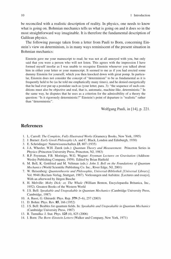
Fig. 2.1 Configuration space for 3 particles in a one-dimensional world

mathematically much nicer to rewrite everything in terms of configuration spacevariables:

q =

⎛⎜⎝

q1...

qN

⎞⎟⎠ ∈ R

3N ,

that is, we write the differential equation for all particles in a compact form as

mq = F , (2.3)

with

F =

⎛⎜⎝

F1...

FN

⎞⎟⎠ ,

and the mass matrix m = (δ ji m j)i, j=1,... ,N .

Configuration space cannot be depicted (but see Fig. 2.1 for a very special situa-tion), at least not for a system of more than one particle, because it is 6-dimensionalfor 2 particles in physical space. It is thus not so easy to think intuitively aboutthings going on in configuration space. But one had better build up some intuitionfor configuration space, because it plays a fundamental role in quantum theory.

A differential equation is by definition a relation between the flow and the vectorfield. The flow is the mapping along the solution curves, which are integral curvesalong the vector field (the tangents of the solution curves). If a physical law is givenby a differential equation, the vector field encodes the physical law. Let us see howthis works.

2.2 Hamiltonian Mechanics 15

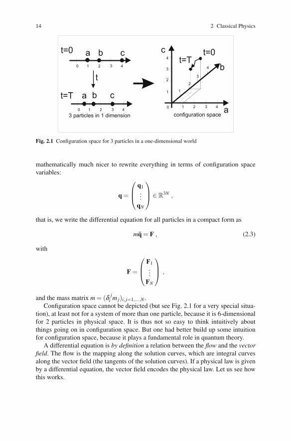
Fig. 2.2 Phase space descrip-tion of the mathematicallyidealized harmonically swing-ing pendulum. The possibletrajectories of the mathemat-ically idealized pendulumswinging in a plane withfrequency 1 are concentriccircles in phase space. Thesets M und M(t) will bediscussed later

(

(.

.

The differential equation (2.3) is of second order and does not express the rela-tion between the integral curves and the vector field in a transparent way. We needto change (2.3) into an equation of first order, so that the vector field becomes trans-parent. For this reason we consider the phase space variables

(qp

)=

⎛⎜⎜⎜⎜⎜⎜⎜⎜⎝

q1...

qN

p1...

pN

⎞⎟⎟⎟⎟⎟⎟⎟⎟⎠∈ R

3N ×R3N = Γ ,

which were introduced by Boltzmann,1 where we consider positions and velocities.However, for convenience of notation, the latter are replaced by momenta pi = mivi.One point inΓ represents the present state of the entire N-particle system. The phasespace has twice the dimension of configuration space and can be depicted for oneparticle moving in one dimension, e.g., the pendulum (see Fig. 2.2).

Clearly, (2.3) becomes

1 The notion of phase space was taken by Ludwig Boltzmann (1844–1906) as synonymous withthe state space, the phase being the collection of variables which uniquely determine the physicalstate. The physical state is uniquely determined if its future and past evolution in time is uniquelydetermined by the physical law.

16 2 Classical Physics

(qp

)=

(m−1pF(q)

). (2.4)

The state of the N-particle system is completely determined by

(qp

), because (2.4)

and the initial values

(q(t0)p(t0)

)uniquely determine the phase space trajectory (if the

initial value problem allows for a solution).For (2.2) and many other effective forces, there exists a function V on R

3N , theso called potential energy function, with the property that

F =−gradqV =−∂V∂q

=−∇V .

Using this we may write (2.4) as

(qp

)=

⎛⎜⎜⎝∂H∂p

(q,p)

−∂H∂q

(q,p)

⎞⎟⎟⎠ , (2.5)

where

H(q,p) =12(p ·m−1p)+V (q)

=12

N

∑i=1

p2i

mi+V (q1, . . . ,qN) . (2.6)

Now we have the Newtonian law in the form of a transparent differential equation(2.5), expressing the relation between the integral curves (on the left-hand side,differentiated to yield tangent vectors) and the vector field on the right-hand side(which are the tangent vectors expressing the physics). The way we have writtenit, the vector field is actually generated by a function H (2.6) on phase space. Thisis called the Hamilton function, after its inventor William Rowan Hamilton (1805–1865), who in fact introduced the symbol H in honor of the physicist ChristiaanHuygens (1629–1695). We shall see later what the “wave man” Huygens has to dowith all this. The role of the Hamilton function H(q,p) is to give the vector field

vH(q,p) =

⎛⎜⎜⎝∂H∂p

−∂H∂q

⎞⎟⎟⎠ , (2.7)

and the Hamiltonian dynamics is simply given by

2.2 Hamiltonian Mechanics 17

(qp

)= vH(q,p) . (2.8)

The function H allows us to focus on a particular structure of Newtonian mechanics,now rewritten in Hamiltonian terms. Almost all of this section depends solely on thisstructure, and we shall see some examples shortly. Equations (2.5) and (2.6) withthe Hamilton function H(q,p) define a Hamiltonian system.

The integral curves along this vector field (2.7) represent the possible system

trajectories in phase space, i.e., they are solutions

(q(t,(q,p)

)p(t,(q,p)

))

of (2.8) for given

initial values

(q(0,(q,p)

)p(0,(q,p)

))

=(

qp

). Note that this requires existence and unique-

ness of solutions of the differential equations (2.8). One possible evolution of theentire system is represented by one curve in phase space (see Fig. 2.3), which iscalled a flow line, and one defines the Hamiltonian flow by the map (ΦH

t )t∈R fromphase space to phase space, given by the prescription that, for any t, a point in phasespace is mapped to the point to which it moves in time t under the evolution (as longas that evolution is defined, see Remark 2.1):

ΦHt

((qp

))=

(q(t,(q,p)

)p(t,(q,p)

))

.

We shall say more about the flow map later on. The flow can be thought of pictoriallyas the flow of a material fluid in Γ , with the system trajectories as flow lines.

Hamiltonian mechanics is another way of talking about Newtonian mechanics.It is a prosaic way of talking about the motion of particles. The only romance leftis the secret of how to write down the physically relevant H. Once that is done,the romance is over and what lies before one are the laws of mechanics written inmathematical language. So that is all that remains. The advantage of the Hamilto-nian form is that it directly expresses the law as a differential equation (2.8). Andit has the further advantage that it allows one to talk simultaneously about all pos-sible trajectories of a system. This will be helpful when we need to define a typicaltrajectory of the system, which we must do later.

However, this does not by any means imply that we should forget the Newtonianapproach altogether. To understand which path a system takes, it is good to knowhow the particles in the system interact with each other, and to have some intuitionabout that. Moreover, we should not lose sight of what we are interested in, namely,the behavior of the system in physical space. Although we have not elaborated on theissue at all, it is also important to understand the physical reasoning which leads tothe mathematical law (for example, how Newton found the gravitational potential),as this may give us confidence in the correctness of the law. Of course we alsoachieve confidence by checking whether the theory correctly describes what we see,but since we can usually only see a tiny fraction of what a theory says, confidenceis mainly grounded on theoretical insight.

The fundamental properties of the Hamiltonian flow are conservation of energyand conservation of volume. These properties depend only on the form of the equa-

18 2 Classical Physics

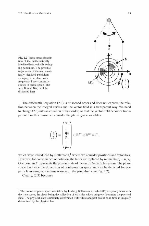
Fig. 2.3 The Hamilton function generates a vector field on the 6N-dimensional phase space of anN-particle system in physical space. The integral curves are the possible trajectories of the entiresystem in phase space. Each point in phase space is the collection of all the positions and velocitiesof all the particles. One must always keep in mind that the trajectories in phase space are nottrajectories in physical space. They can never cross each other because they are integral curves ona vector field, and a unique vector is attached to every point of phase space. Trajectories in phasespace do not interact with each other! They are not the trajectories of particles

tions (2.8) with (2.7), i.e., H(q,p) can be a completely general function of (q,p)and need not be the function (2.6). When working with this generality, one calls pthe canonical momentum, which is no longer simply velocity times mass. Now, con-servation of energy means that the value of the Hamilton function does not changealong trajectories. This is easy to see. Let

(q(t),p(t)

), t ∈ R, be a solution of (2.8).

Then

ddt

H(q(t),p(t)

)= q

∂H∂q

+ p∂H∂p

=∂H∂p∂H∂q− ∂H∂q∂H∂p

= 0 . (2.9)

More generally, the time derivative along the trajectories of any function f(q(t),p(t)

)on phase space is

ddt

f(q(t),p(t)

)= q

∂ f∂q

+ p∂ f∂p

=∂H∂p∂ f∂q− ∂H∂q∂ f∂p

=: { f ,H} . (2.10)

The term { f ,H} is called the Poisson bracket of f and H. It can also be defined inmore general terms for any pair of functions f ,g, viewing g as the Hamilton functionand Φg

t the flow generated by g :

{ f ,g}=ddt

f ◦Φgt =

∂g∂p∂ f∂q− ∂g∂q∂ f∂p

. (2.11)

2.2 Hamiltonian Mechanics 19

Note, that { f ,H} = 0 means that f is a constant of the motion, i.e., the value of fremains unchanged along a trajectory (d f /dt = 0), with f = H being the simplestexample.

Now we come to the conservation of volume. Recall that the Hamiltonian flow(ΦH

t )t∈R is best pictured as a fluid flow in Γ , with the system trajectories as flowlines. These are the integral curves along the Hamiltonian vector field vH(q,p) (2.7).These flow lines have neither sources nor sinks, i.e., the vector field is divergence-free:

divvH(q,p) =(∂∂q

,∂∂p

)⎛⎜⎜⎝∂H∂p

−∂H∂q

⎞⎟⎟⎠ =

∂ 2H∂q∂p

− ∂ 2H∂p∂q

= 0 . (2.12)

This important (though rather trivial) mathematical fact is known as Liouville’s the-orem for the Hamiltonian flow, after Joseph Liouville (1809–1882). (It has noth-ing to do with Liouville’s theorem in complex analysis.) A fluid with a flow that isdivergence-free is said to be incompressible, a behavior different from air in a pump,which gets very much compressed. Consequently, and as we shall show below, the“volume” of any subset in phase space which gets transported via the Hamiltonianflow remains unchanged. Before we express this in mathematical terms and give theproof, we shall consider the issue in more general terms.

Remark 2.2. On the Time Evolution of Measures.The notion of volume deserves some elaboration. Clearly, since phase space is veryhigh-dimensional, the notion of volume here is more abstract than the volume of athree-dimensional object. In fact, we shall later use a notion of volume which is notsimply the trivial extension of three-dimensional volume. Volume here refers to ameasure, the size or weight of sets, where one may in general want to consider abiased weight. The most famous measure, and in fact the mother of all measures,is the generalization of the volume of a cube to arbitrary subsets, known as theLebesgue measure λ . We shall say more about this later.2 If one feels intimidated bythe name Lebesgue measure, then take |A|=

∫A dnx, the usual Riemann integral, as

the (fapp-correct) Lebesgue measure of A. The measure may in a more general sensebe thought of as some kind of weight distribution, where the Lebesgue measuregives equal (i.e., unbiased) weight to every point. For a continuum of points, this isa somewhat demanding notion, but one may nevertheless get a feeling for what ismeant. For the time being we require that the measure be an additive nonnegative setfunction, i.e., a function which attributes positive or zero values to sets, and whichis additive on disjoint sets: μ(A∪B) = μ(A)+ μ(B). The role of the measure will

2 We need to deal with the curse of the continuum, which is that not all subsets of Rn actually

have a volume, or as we now say, a measure. There are non-measurable sets within the enormousmultitude of subsets. These non-measurable sets exist mathematically, but are not constructiblein any practical way out of unions and intersections of simple sets, like cubes or balls. They arenothing we need to worry about in practical terms, but they are nevertheless there, and so must bedealt with properly. This we shall do in Sect. 4.3.1.