Application of Bohmian Mechanics to Quantum Transport: the Conditional Wave Functionbohmmech/... ·...
155
Universit ` a degli Studi di Genova Doctoral Thesis in Physics Cicle XXVII Application of Bohmian Mechanics to Quantum Transport: the Conditional Wave Function Author: Damiano Marian Supervisor: Prof. Nino Zangh` ı External Supervisor: Prof. Xavier Oriols
Transcript of Application of Bohmian Mechanics to Quantum Transport: the Conditional Wave Functionbohmmech/... ·...

Universita degli Studi di Genova
Doctoral Thesis in Physics
Cicle XXVII
Application of Bohmian Mechanics
to Quantum Transport:
the Conditional Wave Function
Author: Damiano Marian Supervisor: Prof. Nino Zanghı
External Supervisor: Prof. Xavier Oriols


Qui delle divertite passioni
per miracolo tace la guerra,
qui tocca anche a noi poveri la nostra parte di
ricchezza
ed e l’odore dei limoni.
Vedi, in questi silenzi in cui le cose
s’abbandonano e sembrano vicine
a tradire il loro ultimo segreto,
talora ci si aspetta
di scoprire uno sbaglio di Natura,
il punto morto del mondo, l’anello che non tiene,
il filo da disbrogliare che finalmente ci metta
nel mezzo di una verita.
Eugenio Montale


Contents
Contents v
Introduction 1
Publications Related to This Thesis 5
1 Bohmian Mechanics 7
1.1 Why Looking for an Alternative to the Orthodox Interpretation of Quan-tum Mechanics? . . . . . . . . . . . . . . . . . . . . . . . . . . . . . . . . 7
1.2 Particles with Definite Positions . . . . . . . . . . . . . . . . . . . . . . . 10
1.3 Conditional Wave Function . . . . . . . . . . . . . . . . . . . . . . . . . . 11
1.4 Quantum Equilibrium Hypotesis, Equivariance and Empirical Equivalence 12
1.5 Can a Clear Theory be Useful for Computing and Understanding Quan-tum Phenomena? . . . . . . . . . . . . . . . . . . . . . . . . . . . . . . . . 13
2 The Many-Body Problem: Use of the Conditional Wave Function 15
2.1 Understanding Collapse . . . . . . . . . . . . . . . . . . . . . . . . . . . . 15
2.1.1 Collapse in the Orthodox Interpretation of Quantum Mechanics . . 16
2.1.2 Theoretical Treatment of Collapse with Bohmian Mechanics . . . . 19
2.2 Dynamical Evolution of the Conditional Wave Function . . . . . . . . . . 25
2.2.1 General Schrodinger-Type Equation for the Conditional Wave Func-tion . . . . . . . . . . . . . . . . . . . . . . . . . . . . . . . . . . . 26
2.2.2 Conditional Wave Function for Separable Quantum Systems . . . . 27
2.3 Numerical Algorithm for Solving Many-Body Problems with the Condi-tional Wave Function . . . . . . . . . . . . . . . . . . . . . . . . . . . . . . 28
2.3.1 The Small Entanglement Approximation . . . . . . . . . . . . . . . 29
2.3.1.1 Numerical Example in the Small Entanglement Approx-imation: Limitation and Validity . . . . . . . . . . . . . . 30
2.3.2 A Practical Algorithm for Solving the Many-Particle SchrodingerEquation . . . . . . . . . . . . . . . . . . . . . . . . . . . . . . . . 33
3 On the Measurement of the Total Current in Quantum Devices 37
3.1 Transmitted Charge Detector . . . . . . . . . . . . . . . . . . . . . . . . . 38
3.1.1 Specifying the System plus Apparatus Schrodinger Equation . . . 39
3.1.2 Derivation of Quantum Hamilton-Jacobi and Continuity Equations 42
3.1.3 The Relationship Between the Total Current on the Ammeter andthe Bohmian Trajectories of the System . . . . . . . . . . . . . . . 44
v
3.1.4 The Many-particle Schrodinger Equation of the System plus Ap-paratus . . . . . . . . . . . . . . . . . . . . . . . . . . . . . . . . . 48
3.1.4.1 Numerical Derivation of the Collapse . . . . . . . . . . . 51
3.1.5 Solving the System plus Apparatus Schrodinger Equation . . . . . 52
3.2 Ammeter for High-Frequency Current . . . . . . . . . . . . . . . . . . . . 55
3.2.1 Any Mean Value of an Observable can be Calculated from Ensem-ble Trajectories . . . . . . . . . . . . . . . . . . . . . . . . . . . . . 56
3.2.2 Simulation with Conditional Wave Function . . . . . . . . . . . . . 57
3.2.2.1 Simulation of the Electrons in the Metal Surface . . . . . 59
3.2.3 Back-Action on the Quantum System . . . . . . . . . . . . . . . . 59
3.2.4 Computations of the Total Current . . . . . . . . . . . . . . . . . . 61
3.2.5 Weak Measurement . . . . . . . . . . . . . . . . . . . . . . . . . . 62
4 Weak Measurement of Bohmian Velocity in Mesoscopic Systems 65
4.1 Weak Measurement of Bohmian Velocity from the Total Electrical Current 66
4.1.1 Theory of Weak Measurement . . . . . . . . . . . . . . . . . . . . . 66
4.1.2 On the Total Current Measured on Different Metallic Surfaces . . 70
4.1.2.1 Total Current on an Large Surface S . . . . . . . . . . . 70
4.1.2.2 Is the Measurement on a Large Surface a Weak Measure-ment? . . . . . . . . . . . . . . . . . . . . . . . . . . . . . 72
4.1.2.3 Total Current on a Small Surface S . . . . . . . . . . . . 73
4.2 Geometry of the Proposed Experiment . . . . . . . . . . . . . . . . . . . . 75
4.2.1 Derivation of Bohmian Velocity Weak Value . . . . . . . . . . . . . 76
4.3 Numerical Experiments . . . . . . . . . . . . . . . . . . . . . . . . . . . . 77
5 Time-Dependent Problems in Quantum Transport 81
5.1 Detection at the Same Place of Two Simultaneously Emitted Electrons . . 81
5.1.1 Two-Particle Probabilities . . . . . . . . . . . . . . . . . . . . . . . 86
5.1.2 Numerical Results . . . . . . . . . . . . . . . . . . . . . . . . . . . 92
5.1.2.1 Two-Particle Scenario with a Separable and SymmetricalDouble Barrier Potential . . . . . . . . . . . . . . . . . . 92
5.1.2.2 Two-Particle Scenario with a Separable and Non-SymmetricalDouble Barrier Potential . . . . . . . . . . . . . . . . . . 94
5.1.2.3 Two-Particle Scenario with Non-Separable Double Bar-rier Potential . . . . . . . . . . . . . . . . . . . . . . . . . 95
5.1.2.4 Two-Particle Scenario with Single Barrier Potential . . . 96
5.1.3 Final Considerations . . . . . . . . . . . . . . . . . . . . . . . . . . 98
5.2 Quantum Noise with Bohmian Mechanics Simulations . . . . . . . . . . . 100
5.2.1 Quantum Noise in Electrical Devices from an Experimental Pointof View . . . . . . . . . . . . . . . . . . . . . . . . . . . . . . . . . 101
5.2.2 Quantum Noise in Electrical Devices from a Computational Pointof View . . . . . . . . . . . . . . . . . . . . . . . . . . . . . . . . . 104
5.2.3 Computational Ability of Bohmian Mechanics in Solving QuantumNoise . . . . . . . . . . . . . . . . . . . . . . . . . . . . . . . . . . 106
5.2.4 Discussion . . . . . . . . . . . . . . . . . . . . . . . . . . . . . . . . 110
A Going Beyond the Small Entanglement Approximation 113

B Analytical Formula for the Electric Flux Through a Surface 119
C Derivation of the Bohmian Velocity Through Weak Measurement Pro-cedure 125
D Analytical Two-Particle Probabilities from the Scattering Formalismwith Mono-Energetic Initial States 129
E Analytical Two-Particle Probabilities for Arbitrary Wave Packets 133
F The Quantum DC Current in Ergodic Systems 137
Bibliography 139


Introduction
This Thesis is aimed to apply Bohmian Mechanics to the study of quantum transport
in mesoscopic systems. Bohmian Mechanics is an alternative version of Quantum Me-
chanics in which particles have a definite position and their motion is choreographed
by the wave function. This theory has been proposed by Louis de Broglie [28] in 1926,
rediscovered independently by David Bohm [28] in 1952 and from the 1980’s developed
and systematized by the research group formed by Detlef Durr, Sheldon Goldstein and
Nino Zanghı [35]. It provides the same statistical results as those of Orthodox Quan-
tum Mechanics for any conceivable experiment in the contest of non-relativistic quantum
phenomena, it solves the famous “Schrodinger cat paradox” (i.e. the measurement prob-
lem), it clarifies the role of operators as observables and it derives the collapse postulate
of the wave function [29, 32].
This theory has always been regarded as useful to solve issues related to the foundational
aspects of Quantum Theory, but otherwise useless. In recent years this has started to
change in the Physics community and some researchers have started to use this theory
to solve practical problems. Around 2000 Robert E. Wyatt and collaborators started to
use Bohmian Mechanics, in particular its hydrodynamical formulation, to solve problems
of kinetic chemistry [54, 84] opening a new research line that has been quite successful
among theoretical chemists. More recently, Xavier Oriols has used Bohmian Mechan-
ics to find an approximate solution to the many-body quantum problem [67] and his
research group has developed the BITLLES simulator for quantum transport in nano-
electronic devices [11]. Salvador Miret-Artes has used this theory for studying classical
and quantum trajectories and Angel Sanz addressing atomic, molecular and optical
physics [73, 74].
It should also be mentioned that, very recently, this theory has attracted some experi-
mental interest. Noteworthily, is the experiment performed by the group of Steinberg,
which has led to a reconstruction of the photon trajectories by means of weak measure-
ments in a double slit set-up; the measured trajectories turn out to be the ones predicted
by Bohmian Mechanics [45].
1

Introduction 2
The present Thesis fits in the wake of the contemporary research aiming at showing the
utility of Bohmian Mechanics in solving practical problems. The notion of conditional
wave function, an exclusive concept of Bohmian Mechanics, is central for explaining
how this theory offers not only different numerical tools for solving the long-standing
many-body problem, but also new unexplored ways to attack and understand complex
quantum problems. In particular, the numerical tools offered by this theory will be
used throughout the thesis to create new strategies for analyzing physical situation in
which it is not completely clear the correct way to proceed. For example, it will be
considered the interaction of an electron with an external apparatus that measures the
High-Frequency total electrical current. One obtains in this way novel way of simulating
and comprehending the effect of an external environment on a quantum system in this
particular regime.
The Thesis is organized as follows. In Chapter 1 the basic notions of Bohmian Mechan-
ics needed for the present Thesis will be presented. It will be motivated why there is a
need to look for an alternative version of Quantum Mechanics, both from a fundamental
and from a practical point of view. In Chapter 2 the use of the conditional wave func-
tion in solving many-body problems will be addressed. First, it will be shown how the
collapse postulate is simply understood and derived within Bohm theory (Section 2.1),
second it will be presented the dynamical evolution of the conditional wave function
(Section 2.2) and finally it will be presented a numerical (approximate) algorithm to
solve many-particle problems (Section 2.3). Chapter 3 is focused on studying the mea-
surement of the total current in quantum devices. Specifically, it will be presented a
model for measuring the successful transmission of an electron impinging on a tunneling
barrier (Section 3.1) and a model for measuring the total electrical current at TeraHertz
frequencies in quantum devices (Section 3.2). In Chapter 4 it will be proposed a way to
measure the Bohmian velocity of an electron in solid-state systems through the notion
of weak measurement. A detailed introduction about weak measurement will be given
(Section 4.1). It will be proposed a possible geometry for a device (Section 4.2) and
a numerical study for understanding the feasibility of the proposed experiment will be
presented (Section 4.3). Finally, in Chapter 5 two different problems will be considered:
first, a numerical and theoretical study of the scattering probabilities in a two-particle
HOM-type (Hong-Ou-Mandel) experiment (Section 5.1) and second, the understanding
the origin of quantum noise within Bohmian Mechanics (Section 5.2).
Six Appendixes complement this Thesis. In Appendix A a path for the development of a
new algorithm for solving the many-particle problem beyond the known approximations
is presented. In Appendix B an analytical derivation of the electric flux through a
surface is provided. Appendix C is devoted to derive analytically the Bohmian velocity
from a weak measurement procedure. In Appendix D and Appendix E the derivation

Introduction 3
of two-particle probabilities for scattering formalism and for generic wave packets are
presented. Appendix F addresses the quantum DC current in ergodic systems.


Publications Related to This
Thesis
• Marian, D., Colomes, E., Zhan, Z. & Oriols, X.
Quantum Noise from a Bohmian perspective: fundamental understanding and
practical computation in electron devices
Journal of Computational Electronics, Special Issue on Noise Modeling, in press
(2015). See also arxiv:1410.0530
• Norsen, T., Marian, D. & Oriols, X.
Can the wave function in configuration space be replaced by single-particle wave
functions in physical space?
Synthese, Special Issue: Space-time and the wave function, 1-27 (2014)
doi: 10.1007/s11229-014-0577-0, see also arxiv:1410.3676
• Colomes, E., Marian, D. & Oriols, X.
Understandable algorithm for exchange interaction: Quantum noise in nanoelec-
tronic devices
Computational Electronics (IWCE), 2014 International Workshop on, 3-6 June
2014
doi: 10.1109/IWCE.2014.6865811
• Marian, D., Zanghı, N. & Oriols, X.
On the back-action of THz measurement on the total current of quantum devices
Computational Electronics (IWCE), 2014 International Workshop on, 3-6 June
2014
doi: 10.1109/IWCE.2014.6865844
• Albareda, G., Marian, D., Benali, A., Alarcon, A., Yaro, S. & Oriols, X.
Book Chapter Electron Devices Simulation with Bohmian Trajectories
in Simulation of transport in nanodevices, Volume 1: Principles, models and meth-
ods, ISTE Ltd (2014).
5

Publications 6
• Albareda, G., Marian, D., Benali, A., Yaro, S., Zanghı, N. & Oriols, X.
Time-resolved electron transport with quantum trajectories
Journal of Computational Electronics, Special Issue on Quantum Transport Be-
yond DC, 12(3), 405-419 (2013).
• Marian, D., Colomes, E. & Oriols, X.
Time-dependent exchange and tunneling: detection at the same place of two elec-
trons emitted simultaneously from different sources
Submitted, see also arxiv:1408.1990
In preparation
• Marian, D., Oriols, X. & Zanghı, N.: Proposal for Measuring the Bohmian Velocity
in Mesoscopic Systems using the Weak Value of the Total Electrical Current.

Chapter 1
Bohmian Mechanics
1.1 Why Looking for an Alternative to the Orthodox In-
terpretation of Quantum Mechanics?
Orthodox Interpretation of Quantum Mechanics is undoubtedly one of the most success-
ful theories in Physics. It has been tested in several situations and its predictions allowed
the discovering of new and surprising phenomena; however its foundational aspects have
been matter of debate since its appearing. The reason why Orthodox Interpretation
exhibits foundational problems resides essentially on what Erwin Schrodinger has ad-
dressed in his famous 1935 paper The Present Situation in Quantum Mechanics [77],
commonly known as the Schrodinger “cat paradox” paper
One can even set up quite ridiculous cases. A cat is penned up in a steel
chamber, along with the following diabolic device (which must be secured
against direct interference by the cat): in a Geiger counter there is a tiny
bit of radioactive substance, so small, that perhaps in the course of one hour
one of the atoms decays, but also, with equal probability, perhaps none; if it
happens, the counter tube discharges and through a relay releases a hammer
which shatters a small flask of hydrocyniac acid. If one has left this entire
system to itself for an hour, one would say that the cat still lives if meanwhile
no atom has decayed. The first atomic decay would have poisoned it. The
ψ-function of the entire system would express this by having in it the living
and the dead cat (pardon the expression) mixed or smeared out in equal
parts.
It is typical of these cases that an indeterminacy originally restricted to the
atomic domain becomes transformed into macroscopic indeterminacy, which
7
Chapter 1. Bohmian Mechanics 8
can then be resolved by direct observation. That prevents us from so naively
accepting as valid a “blurred model” for representing reality. In itself, it
would not embody anything unclear or contradictory. There is a difference
between a shaky or out-of-focus photograph and a snapshot of clouds and
fog banks.[77]
The cat’s example expresses essentially the concept that the “blurring” of the micro-
scopic description, represented by the wave function, emerges, in a quite embarrassing
way, into the macroscopic scale. If this “blurring” is confined to the microscopic scale,
where one has no direct control, it is acceptable,
But serious misgivings arise if one notices that the uncertainty affects macro-
scopically tangible and visible things, for which the term “blurring” seems
simply wrong.[77]
The very same problem expressed by Schrodinger was also addressed by Albert Einstein
in the volume Albert Einstein, philosopher-scientist [75]. While describing a radioactive
atom, he reflects about the exact instant in which it decays. Exactly as Schrodinger
he considers the situation in which, along with the atom, the instrument that certifies
the decay of the atom, for example a Geiger counter, is included. Moreover, he includes
a registration strip upon which a mark is made. This system is very complex and its
configuration is of very high dimension, but nevertheless can be in principle treated
quantum mechanically. If enough time is awaited, i.e. enough to be sure that the mark
on the strip has been made, the wave function of the composed system is spread over all
the microscopic configurations that correspond to the different marks’ positions on the
strip. But the wave function does not contain the definite location of the mark actually
occurred. About this argumentation Einstein comments:
In this consideration the location of the mark on the strip plays the role
played in the original consideration by the time of disintegration. The rea-
son for the introduction of the system supplemented by the registration-
mechanism lies in the following. The location of the mark on the registration-
strip is a fact which belongs entirely within the sphere of macroscopic con-
cepts, in contradistinction to the instant of disintegration of a single atom.[75]
Then he reaches the conclusion that
If we attempt [to work with] the interpretation that the quantum-theoretical
description of the individual system we are forced to the interpretation that

Chapter 1. Bohmian Mechanics 9
the location of the mark on the strip is nothing which belongs to the system
per se, but that the existence of that location is essentially dependent upon
the carrying out of an observation made on the registration strip.[75]
This is basically the lesson of the so called Orthodox Interpretation (also known as
Copenhagen Interpretation of Quantum Mechanics or Ordinary Quantum Mechanics),
settled down by Bohr [19] and Heisenberg [42] around 1927: the act of observing is
responsible of the mark on the strip being in a place or in another (or in the cat’s
example of its being dead or alive). Einstein continues:
Such an interpretation is certainly by no means absurd from a purely logical
standpoints; yet there is hardly likely to be anyone who would consider it
seriously.[75]
The problem previously exposed, using the words of Schrodinger and Einstein, is com-
monly known as the “measurement problem” which is somehow regarded as “the prob-
lem” of the Orthodox Interpretation of Quantum Mechanics. Also Richard Feynman
was disappointed and somehow embarrassed by the fact that the act of observation has
such a central role in the Orthodox Interpretation
This is all very confusing, especially when we consider that even tough we
may consistently consider ourselves always to be the outside observer when
we look at the rest of the world, the rest of the world is at the same time
observing us, and that often we agree on what we see in each other. Does
this mean that my observations become real only when I observe an ob-
server observing something as it happens? This is an horrible viewpoint. Do
you seriously entertain the thought without the observer there is no reality?
Which observer? Any observer? Is a fly an observer? Ia a star an observer?
Was there no reality in the universe before 109 B.C. when life began? Or are
you the observer? Then there is no reality to the world after you are dead?
I know a number of otherwise respectable physicists who have bought life
insurance.[37]
Ultimately the “measurement problem” is a reflection of a fundamental ambiguity present
in the formulation of the orthodox theory of quantum mechanics. Using the words of
John Stewart Bell, one realizes that
Nobody knows what quantum mechanics says exactly about any situation, for
nobody knows where the boundary really is between wavy quantum systems
and the world of particular events.[9]

Chapter 1. Bohmian Mechanics 10
Then it emerges clearly from the previous quotation that what is ambiguous in the
Orthodox Interpretation of Quantum Mechanics, and what is actually the point undi-
gestible to Schrodinger, Einstein and Feynamn, is the undefined line that separates the
macroscopic and microscopic world: the Schrodinger’s cat is nothing else than a mani-
festation of this fundamental ambiguity in the theory.
During the last fifty years many different theories have been proposed to solve the
problem exposed above, only to name a few: Bohmian Mechanics [15, 35, 68], Ghirardi-
Rimini-Weber theory [38] and Many Worlds Interpretation [36]. Each theory solves
the measurement problem in a different way but all have a common character: ob-
server, observation, measurement etc. do not play any fundamental role in the theory.
Bohmian Mechanics says that the wave function is not everything and adds to it defi-
nite positions for the particles; Ghirardi-Rimini-Webber theory (or its variants known
as Spontaneous Collapse Models) provides a different dynamical evolution for the wave
function, introducing a stochastic process responsible for the collapse of the wave func-
tion at macroscopic scale while maintaing usual Schrodinger dynamics at microscopic
level; Many Worlds Interpretation assumes that at every splitting of the wave function
there actually exist two different worlds, in the Schrodinger example, one with the dead
cat and the other with the alive cat. Ghirardi-Rimini-Webber theory and Many Words
Interpretation will not be treated in the present thesis, while in the following of this
Chapter the principal characteristics of Bohmian Mechanics will be presented.
1.2 Particles with Definite Positions
The main idea of Bohmian Mechanics is to insist when saying particles to mean particles:
particles follow trajectories, i.e. they have always definite positions in space at a given
time. In this theory the wave function evolves according to (the usual) Schrodinger
equation
i~∂Ψ(x1, x2, · · · , xN , t)
∂t= HΨ(x1, x2, · · · , xN , t), (1.1)
where H = −∑N
i=1~2
2mi∂2
∂x2i
+ V (x1, x2, · · · , xN , t) is the usual Hamiltonian composed
by a free part and a general interacting potential V . The wave function guides the
particles motion through the so-called guidance law : for a system of N particles whose
configuration at time t is X(t) = (X1(t), X2(t), ..., XN (t)), where Xi(t) denotes the
actual potions of particle i at time t in the physical space, it reads

Chapter 1. Bohmian Mechanics 11
dXi(t)
dt= vi|x=X(t) =
~mi
ImΨ∗∇iΨ
Ψ∗Ψ
∣∣∣x=X(t)
, (1.2)
where mi is the mass of particle i, Im denotes the imaginary part, and ∇i the gradient
relative to the 3 coordinates of particle i.1 Equation (1.2) is written to be valid both
for particles with spin and without spin. For the former the wave function is a spinor
Ψ : R3N → Ck, i.e. a function of the configuration with k complex components, then
Ψ∗Ψ is the scalar product in Ck. For the latter the wave function is complex-valued, i.e.
Ψ : R3N → C, then in Equation (1.2) the term Ψ∗ cancels out.
Since Equation (1.1) does not involve the configuration of the particles X(t), its solution
is unique once the initial wave function Ψ0 at time t = t0 is specified. Note that
Equation (1.2) consists of 3 components of particle i out of 3N component of the vector
field vΨ on configuration space R3N . Then Equation (1.2) can be summarized, for
i = 1, ..., N as
dX(t)
dt= vΨ(X(t)). (1.3)
Because Ψ is known from Equation (1.1), once the initial configuration is specified X(t0),
Equation (1.3) determines the history of the configuration X(t). Hence Bohmian Me-
chanics is a deterministic theory: once Ψ0 and X(t0) are specified the entire history is
determined by Equations (1.1) and (1.2). The state of the system in Bohmian Mechanics
is then completely specified by the pair (X(t),Ψ) at any time.
1.3 Conditional Wave Function
The conditional wave function is a unique tool belonging to Bohmian Mechanics, it
is a precise and unambiguous definition of the wave function of a subsystem. Con-
sider N interacting quantum particles (a close system, ultimately the entire universe)
described by their wave function Ψ(x1, x2, ..., xN , t) and their configuration X(t) =
(X1(t), X2(t), ..., XN (t)), the wave function of particle 1 is simply given by fixing all
the actual positions of the remaining particles
1In the present thesis a bold variable indicates a point in the configuration space, while a non-boldvariable indicates a point in the physical space. Capital letters denote the actual positions of particles,while lowercase letters denote generic positions.
Chapter 1. Bohmian Mechanics 12
ψ1(x1, t) = Ψ(x1, x2, ..., xN , t)|x2=X2(t),...,xN=xN (t) = Ψ(x,X2(t), ..., XN (t), t). (1.4)
Note that the conditional wave function of Equation (1.4) depends on time in two dif-
ferent ways; the usual time dependence plus the time dependence on the other particles
positions (X2(t), ..., XN (t)). In the same way it is possible to define the wave function
of all the other particles, for example particle’s 2 conditional wave function is simply:
ψ2(x2, t) = Ψ(X1(t), x2, X3(t), ..., XN (t), t). An important consequence of the definition
of the conditional wave function given by Equation (1.4) is that Equation (1.2) may be
re-written, for each particle, in terms of its associated conditional wave function
dXi(t)
dt=
~mi
Im∇iΨ
Ψ
∣∣∣x=X(t)
=~mi
Im∇ψiψi
∣∣∣xi=Xi(t)
. (1.5)
Thus, in order to obtain the trajectories of the N particles it is only needed, in principle,
to know which is the conditional wave function of each particle. The conditional wave
function is a central object in the developing of the present Thesis; its characteristics
will be described in details in Chapter 2 and will be used throughout the Thesis.
1.4 Quantum Equilibrium Hypotesis, Equivariance and Em-
pirical Equivalence
Bohmian Mechanics makes the same empirical prediction of Ordinary Quantum Mechan-
ics, whenever the latter is non-ambiguous. In fact, the right hand side of the guidance
equation (1.2) can be understood as vi = ji/ρ, evaluated at the configuration point
X(t), where ji is the standard probability current associated with particle i and ρ is the
standard probability density. As consequence of Equation (1.1), the probability current
and density obey the continuity equation
∂ρ
∂t+∑i
∇iji = 0. (1.6)
If one considers an ensemble of systems with the same wave function Ψ but random
configurations X moving with configuration-space velocity v, it is easy to see that the
probability distribution P (X, t) over the ensemble should evolve according to

Chapter 1. Bohmian Mechanics 13
∂P
∂t+∑i
∇i(Pvi) = 0. (1.7)
Comparison with Equation (1.6) shows that, since vi = ji/ρ, P = ρ is a solution. Thus,
if the initial configurations X(t0) in the ensemble are chosen with distribution P [X(t0) =
x] = ρ(x, t0) = Ψ∗(x, t0)Ψ(x, t0) - the so-called quantum equilibrium hypothesis - it is
then a consequence of Equations (1.1) and (1.2) jointly that
P [X(t) = x] = ρ(x, t) = Ψ∗(x, t)Ψ(x, t) (1.8)
for all t. It is thus clear that Bohmian mechanics reproduces the statistical predictions
of Ordinary Quantum Mechanics for position measurements, and hence also for any
other type of measurement whose outcome is ultimately registered in the position of
some pointer. This means that Bohmian mechanics is empirically equivalent to Ordi-
nary Quantum Mechanics, thus the two theories can not be tested against each other.
1.5 Can a Clear Theory be Useful for Computing and Un-
derstanding Quantum Phenomena?
After having exposed the principal features of Bohmian Mechanics it is important to
come back to the question posed in the title of Section 1.1: Why looking for an alter-
native to the Orthodox Interpretation of Quantum Mechanics? As briefly exposed, this
theory is an alternative version of Quantum Mechanics that does not need any con-
cept of observer or observation in its foundations, it provides a clear and unambiguous
way to define the wave function of a subsystem and clearly explains the results of any
conceivable experiment giving the same empirical predictions of the Ordinary Quantum
Mechanics (whenever the latter is non-ambiguous).
There exists another reason, at least for the author of the present thesis, for considering
an alternative version of Quantum Mechanics: It could provide new “practical applica-
tions” going beyond of those of standard framework. This is exactly the main subject of
the present thesis. With “practical application” is intended any support of the theory
in order to solve specific problems (such as: the interaction of a small quantum sys-
tem with an external environment; the solution of a numerical inaccessible problem, as

Chapter 1. Bohmian Mechanics 14
for example the many-particle Schrodinger equation, by means of new tools and new
approximations, etc.), to deeply investigate the physical origin of quantum phenomena
inside of the theory (for example noise in quantum transport) and to attack some very
complex problems in a direct and unambiguous way without the introduction of addi-
tional postulates (such as: the famous “collapse postulate” of the wave function; the
introduction of ad-hoc “operators” for some particular experiments, etc.).
Stepping back to the last quotation used at the end of Section 1.1, when summarizing
what Bell calls the first class problem of quantum theory (such as the measurement
problem, the awkward notions of operator, measurement, observer etc.), he continues
This is the first class problem and, as we all know, it does not matter at all in
practice. [...] It doesn’t matter in practice and it is very much a question of
debate among physicists whether or not you should worry about a question
of principle before it becomes a question of practice.[9]
The present work somehow contradicts this last statement: It could be the case that a
(ontologically) clear theory becomes relevant for questions of practice, especially in all
the situations where “nobody knows what quantum mechanics says exactly”[9]. In fact,
if the problem on the foundation of quantum theory was the fundamental ambiguity
on the division between the classical and quantum world, nowadays many experiments,
applications etc. are exactly performed in the boundary of this two worlds: A complete
and non-ambiguous theory allows to describe these situations in a clear and perhaps
intuitive way. In the specific case of Bohmian mechanics, the notion of conditional wave
function becomes fundamental to study these physical regimes and this is why it is the
main object of the present thesis.

Chapter 2
The Many-Body Problem: Use of
the Conditional Wave Function
Ordinary Quantum Mechanics usually does not attribute a wave function for a single
part of a larger quantum mechanical system. The standard way to proceed is to trace out
certain degrees of freedom ending up with the so-called reduced density matrix. Instead
Bohmian Mechanics uses the notion of conditional wave function already introduced in
Section 1.3. The present Chapter is devoted to analyze the main characteristics of this
quantum mechanical object with a particular attention to its usefulness in understanding
many-body problems. It will be explained its role in the derivation of the so called
collapse postulate, its dynamical evolution and its practical use for solving many-particle
quantum problems. In this Chapter to simplify the discussion, spinless particles will be
considered. All the discussion can be reformulated for particles with spin using the
notion of conditional density matrix [33].
2.1 Understanding Collapse
The first many-body problem considered is the interaction of a quantum system with
an apparatus. As already explained in Chapter 1, in Bohmian Mechanics there is no
separation between “measuring apparatus” and a “quantum system”, both are treated at
the same footing, taking care that a suitable interaction between them is modeled. While
analyzing this interaction some interesting feature of the conditional wave function will
be addressed. In particular, as it will be seen in more detail later in the present Chapter,
the conditional wave function obeys the usual one-particle Schrodinger equation in the
expected type of situation in which the particle in question is suitably isolated from
its environment. Nevertheless in general (when there is non-trivial interaction among
15

Chapter 2. The Many-Body Problem 16
particles) the conditional wave function will evolve in an unusual (non-unitary) way. To
give a sense of the possible behavior and also to provide a sense of how the measurement
axioms of ordinary Quantum Mechanics can instead be derived, from a careful analysis
of appropriate kinds of interactions in Bohmian Mechanics, it will be explained how
the one-particle wave function associated with a quantum system collapses when there
is a proper interaction with another system such as a measuring device. First it will
be exposed how ordinary quantum theory deals with a measurement process with the
introduction of the collapse of the wave function postulate, then the derivation of the
collapse within Bohmian Mechanics with a simple analytically-solvable toy model will be
illustrated in details. The discussion of the collapse will be done in a practical situation:
the transmission of an electron impinging upon a tunneling barrier.
2.1.1 Collapse in the Orthodox Interpretation of Quantum Mechanics
As already said in Chapter 1 the Orthodox Interpretation associates only a wave func-
tion to a physical system. Within the first non-relativistic quantization language, the
evolution of this wave function is defined by a law and a postulate. The law is the
usual Schrodinger equation, which states that (when the system is not measured) the
wave function evolves unitarily and deterministically. The postulate provides the col-
lapse of the wave function when a measurement on the physical system is performed.
Its enunciate can be found in many textbooks, as for example in the Cohen-Tannoudji
[22]:
If the measurement of physical quantityA on the system in the state |Ψ〉 gives
result an, the state of the system immediately after the measurement is the
normalized projection Pn|Ψ〉√〈Ψ|Pn|Ψ〉
, of |Ψ〉 onto the eigensubspace associated
with an
where an is the eigenvalue of the corresponding operator A which describes the physical
quantity A and Pn is the projection operator onto the subspace Hn of the total Hilbert
space H. This means that once it is measured (and not before), the system gets fully
projected to one of the eigenstates in a non-unitary evolution. After the collapse, the
new wave packet evolves again according to the time-dependent Schrodinger equation
until a new measurement is done.
This postulate requires a new non-unitary operator A (different from the Hamiltonian
which is present in the Schrodinger equation) able to encapsulate all the interactions
of the quantum systems with the rest of the particles. This operator is the only tool
through which the possible results of a measurement can be determined. In principle

Chapter 2. The Many-Body Problem 17
(a) t = 0
(b) Interaction
with the barrier
(c) t = t₁
(d) t = t₂
Barrier
Electron Position x (nm)
Squ
ared
Mo
du
lus
of
Wav
e F
un
ctio
n (
a.u
.)
-400 -300 -200 -100 0 100 200 300 400
Figure 2.1: Evolution of the squared modulus of the wave function of an electronimpinging on a tunneling barrier (green solid line). Four different times are plottedcorresponding to (a) initial time, (b) the moment when the wave function interactswith the barrier, (c) the time t1 when it occurs the first measurement and (d) time t2corresponding to the second measurement. At time t1 and t2, because of the unitary
evolution, the electron can be detected at both sides of the barrier.
nothing is known about this operator except that it is a (hermitian A = A†) function
whose (real) eigenvalues an of its spectral decomposition are the possible results of the
measurement.
Why the collapse postulate is necessary within the orthodox quantum theory is briefly
explained in the following example: Imagine to have a typical scenario in which an
electron is impinging upon a partially transparent barrier. Electron transport through
the barrier takes place by tunneling. Electron is either transmitted or reflected, but not
both! [16, 24, 61] An electron is transmitted with a probability T , while is reflected with
probability R = 1− T . Each electron, after measurement, will appear randomly at the
left or the right of the barrier. In the idealized situation just considered the electron wave
function can be modeled as one dimensional, Ψ(x, t), where x is the transport direction.
In Figure 2.1 the (unitary) evolution of such wave function solution of Equation (1.1)

Chapter 2. The Many-Body Problem 18
(a) t = 0
(b) Interaction
with the barrier
(c) t = t₁
(d) t = t₂
-400 -200 0 200 -400 -200 0 200 400400
(e) t = 0
(f) Interaction
with the barrier
(g) t = t₁
(h) t = t₂
Electron Position x (nm)
Squ
ared
Mo
du
lus
of
Wav
e F
un
ctio
n (
a.u
.)
Figure 2.2: (a), (b), (c) and (d) Non unitary evolution of the wave function for areflected electron detected at time t1 on the left side. (e), (f), (g) and (h) Non unitaryevolution of the wave function for a transmitted electron detected at time t1 on the
right side. Symbols are the same of Figure 2.1
is reported. In the one particle Schrodinger equation, it is assumed that the potential
barrier V (x) is centered at x = 0 and different from zero only for −b/2 < x < b/2,
where b is the width of the barrier. In Figure 2.2 the evolution of the same electron, but
undergoing a measurement at time t = t1 after the interaction with the barrier, is plotted.
For simplicity, in the present conceptual discussion a reasonable (but ad-hoc) operator
is assumed. Such operator provides the following perturbation of the wave function. If
the electron is randomly measured as a reflected electron at t1, the transmitted part
of the wave function is eliminated. This measuring process corresponds to Figures 2.2
(c) and (d) where only the reflected wave function survives after t1. Equivalently, the
measurement process associated to a transmitted electron corresponds to eliminating
the reflected part, as seen in Figures 2.2 (g) and (h).1
1The measurement described in most textbooks is called “projective” (strong) measurement. Thereexists, for example, another type of measurement known as weak measurement, which is useful to describesituations where the effects of the apparatus on the measured system is just a small perturbation. Thelatter will be analyzed in details in Chapter 4.

Chapter 2. The Many-Body Problem 19
Now, by comparing the evolutions of the wave functions in Figure 2.1 and Figure 2.2, it
is obvious that the former is not enough to describe the evolution of the electron wave
function undergoing to a measurement process. By looking at Figure 2.1, it could be the
case that an electron found at time t1 on the right (transmitted) can be found in a later
time t2 on the left as a reflected electron (see the evolution of the probability density
in Figure 2.1). This sequence of probabilities is wrong. Experimental results confirm
that once, say time t1, the electron is detected at one side, in a later time t2 it is always
found at the same side. Then, one gets a very valuable lesson from the Copenhagen
explanation: the (unitary) Schrodinger equation alone is not enough, it is necessary to
introduce the collapse (postulate) of the wave function.
The collapse postulate ultimately implies the introduction of an operator A, which
varies from experiment to experiment, able to get the correct experimental results. It
is important to say that over the years, physicists have identified the operators, by
developing instincts on which are the effects of measurements on the wave function.
There are scenarios (as the one depicted in Figure 2.2) where is quite obvious which
operator is the right one. On the contrary, for example, when measuring the total
(conduction plus displacement) current it is not at all obvious which are the relevant
operators. Is this measurement process continuous or instantaneous? Does it provide
a strong or a weak perturbation of the wave function? The answers to these questions
are certainly not simple. Bohmian Mechanics provides a clear answer to these technical
questions on how to find the right operator. In Chapter 3 this problem will be addressed
in details; for the moment it is enough to focus only on the collapse of the wave function
when system is undergoing a measurement. The following subsection is dedicated to
expose the theoretical treatment of the collapse within Bohmian Mechanics.
2.1.2 Theoretical Treatment of Collapse with Bohmian Mechanics
In the following to facilitate the discussion, the simplest possible multi-particle system
is taken: two spinless particles moving in one spatial dimension. Suppose that particle
1 is “the quantum system to be measured” and particle 2 represents the center of mass
coordinate of the macroscopic pointer of a measuring device associated with quantum
mechanical operator A. Suppose the full system is initially in a product state
Ψ(x1, x2, 0−) = χ(x1)φ(x2) (2.1)
where χ(x1) is an arbitrary linear combination of A eigenstates

Chapter 2. The Many-Body Problem 20
χ(x1) =∑n
cnχn(x1) with Aχn(x1) = anχn(x1) (2.2)
and φ(x2) is a narrow gaussian packet centered at x2 = 0 representing the measuring
device in its ready state.
In a realistic description of a measurement, the “quantum system” and the “measuring
device” would need to interact in a way that drives the wave function Ψ into a set of
macroscopically-disjoint channels in the configuration space, with each channel corre-
sponding to a distinct perceivable possible outcome of the measurement. In the context
of the present simplified two-particle toy-model, the overall idea can be adequately cap-
tured by positing, for example, an impulsive interaction Hamiltonian like
H = λ δ(t)APx2 (2.3)
where px2 is the momentum operator for the pointer.2
In the special case that the “quantum system” happens already to be in an eigenstate
χm of A, this interaction leaves the two-particle system in the state Ψ(x1, x2, 0+) =
χm(x1)φ(x2 − λam). In light of the quantum equilibrium hypothesis (Section 1.4), it
thus follows that the the actual position X2 of the pointer will, with unit probability, lie
near the value λam indicating the pre-measurement (eigen)value am of A. The pointer,
in short, points to the value normally associated with A in this situation. In the general
case, however, the interaction Hamiltonian takes the state in Equation (2.1) to
Ψ(x1, x2, 0+) =
∑n
cnχn(x1)φ(x2 − λan) (2.4)
in which the pointer is in an entangled superposition with the system. This final state
reflects the notorious measurement problem of Ordinary Quantum Mechanics. But for
the Bohmian theory, there is no problem: the empirically observed outcome is not to
be found in the wave function, but instead in the actual final pointer position X2(0+).
Again in light of the quantum equilibrium hypothesis, this will, with probability |cn|2, be
near the value λan indicating that the outcome of the measurement was an.3
2The interaction Hamiltonian in Equation (2.3) was firstly introduced by von Neumann [82] to de-scribe exactly the measurement situation in orthodox quantum theory.
3It is assumed here that the spacing, |λ(an − an+1)|, between adjacent possible pointer positions issmall compared to the width, w, of φ.

Chapter 2. The Many-Body Problem 21
Now consider how the conditional wave function for the “quantum system” evolves
during the measurement. Prior to the interaction, when the joint two-particle wave
function is still given by Equation (2.1), the conditional wave function for particle 1 is
ψ1(x1, 0−) = χ(x1)φ(x2)
∣∣x2=X2(t)
∼∑n
cnχn(x1). (2.5)
This corresponds to the initial superposed wave function that would be attributed to
the “quantum system” in Ordinary Quantum Mechanics. But the post-interaction Ψ,
given by Equation (2.4), involves disjoint channels of support in the configuration space.
The final pointer position, X2(0+), will randomly (depending on the initial conditions)
end up in the support of just one of these channels. That is, φ(x2 − λan)|x2=X2(0+) will
(approximately) vanish for all n except the particular value, n′, satisfying X2(0+) ≈λan′ , which corresponds to the actual result of the measurement. And so the post-
interaction conditional wave function for particle 1 will be
ψ1(x1, 0+) =
∑n
cnχn(x1)φ(x2 − λan)∣∣x2=X2(0+)
∼ χn′(x1). (2.6)
That is, the interaction causes the initially superposed wave function for particle 1 to
collapse to the appropriate eigenfunction (corresponding to the realized outcome of the
measurement) even though the wave function of the joint system evolves exclusively
unitarily according to the two-particle Schrodinger equation. Bohmian Mechanics thus
explains, from the point of view of a theory in which all particles are treated in a fully uni-
form and fully quantum way, how the wave functions of sub-systems may evolve exactly
as described (at the price of non-uniform treatment and additional ad hoc postulates)
in Ordinary Quantum Mechanics.
It is interesting to analyze the same physical situation considered in Section 2.1.1 from
the Bohmian perspective. An electron impinges on a tunneling barrier and its wave
function is partially reflected, with probability R, and partially transmitted, with prob-
ability T = 1−R. Again one of the most simple multi-particle system one can consider is
composed of two degrees of freedom. The interaction can be provided by Equation (2.3)
with the specification of the quantum mechanical operator A as follows:
A ≡ A(x1) = Θ(x1)−Θ(−x1), (2.7)

Chapter 2. The Many-Body Problem 22
Squared Modulus of C
ond. Wave Func. (a.u.)
Electron Position x (a.u.) 1
0 0
0
0
0
0
Poin
ter P
ositi
on x
(a.
u.)
2
Barrier Barrier
Transmitted !Electron
Cond. Wave Func ⎮𝜒 ⎮²T
(a) t = 0
(b) Interaction with the barrier
(c) t = t₁
(d) t = t₂
(e) t = 0
(f) Interaction with the barrier
(g) t = t₁
(h) t = t₂
Wave Function Pointer + Electron in Configuration Space
Electron Conditional Wave Function in Physical Space
Figure 2.3: a), b), c) and d) Schematic evolution of the modulus square of the wavefunction Ψ(x1, x2, t) of the many particle system in the configuration space. a) Timet = 0 the electron is located at the left of the barrier and the pointer is the “ready” statex2 = 0. b) The electron suffer interaction with the barrier. c) and d) Interaction withthe pointer shows up. The horizontal line corresponds to the cut in the configuration
space which defines the conditional wave function of the electron.e), f), g) and h) Evolution of the conditional wave function for a transmitted electron.It is clearly shown that at times t = t1 and t = t2 survives only the transmitted part
of the electron wave function.
where Θ(x) is the Heaviside step function, thus providing an operator that attributes
eigenvalue −1 if the particle is reflected and eigenvalue +1 if the particle is transmitted.
In Figure 2.3 it is considered an initial wave function of the complete system pointer
plus electron at time t = 0 as a product of two single particle wave function as in
Equation (2.1). The interaction Hamiltonian Equation (2.3) is activated from time
t = t1 till time t = t2, namely the system is electron is measured in this interval of time.
In this schematic example the measurement can be modeled as a projective measurement
if the following relation is satisfied:
λ∆t∆a� 1, (2.8)

Chapter 2. The Many-Body Problem 23
where ∆t = t2 − t1 is the interval of the interaction and ∆a = aT − aR is the difference
between the two eigenvalues of the operator A(x1) in Equation (2.7). The wave function
of the electron after the interaction with the barrier in Figure 2.3 can be written as:
χ(x1) = χT (x1) + χR(x1), (2.9)
thus the action of the operator in Equation (2.3) on the eigenvectors of the wave function
in Equation (2.9) is
A(x1)χT (x1) = aTχT (x1) with aT = +1,
A(x1)χR(x1) = aRχR(x1) with aR = −1. (2.10)
The complete wave function Ψ at time t < t1 is
Ψ(x1, x2, t < t1) = [χT (x1) + χR(x1)]φ(x2). (2.11)
When the measurement is performed the wave function is shifted in the pointer direction
x2 forming an entangled superposition of the form
Ψ(x1, x2, t > t1) = χT (x1)φT (x2) + χR(x1)φR(x2). (2.12)
Because Bohmian Mechanics in addition to the wave function posited definite positions
for the particle, one has that the electron position will be in one of the two channels
in the configuration space depicted in Figure 2.3 c) and d). In that specific case the
electron is transmitted thus the pointer moves up. It is important to underline how
trivially the measurement is explained within Bohmian Mechanics, only a channelized
(unitary) time-evolution of 2D wave function plus two Bohmian trajectories, one for the
electron and another for the measuring apparatus are needed. Already at this level the
“measurement problem” exposed in Chapter 1 has completely disappeared: because in
each run of the experiment the electron is either transmitted or reflected (never both!),
the pointer has always a definite position (moving up or moving down). Thus stepping
back to the famous “cat paradox” problem, the paradox does not simply exist: the cat
is always dead or alive!
It is now quite trivial to derive the collapse for the conditional wave function of the
electron, in the case of Figure 2.3 one has:

Chapter 2. The Many-Body Problem 24
Electron Position x (a.u.)
Squared Modulus of C
ond. Wave Func. (a.u.)
1
0 0
0
0
0
0
Poin
ter P
ositi
on x
(a.
u.)
2
Barrier Barrier
Reflected !Electron
Cond. Wave Func ⎮𝜒 ⎮²R
(a) t = 0
(b) Interaction with the barrier
(c) t = t₁
(d) t = t₂
(e) t = 0
(f) Interaction with the barrier
(g) t = t₁
(h) t = t₂
Wave Function Pointer + Electron in Configuration Space
Electron Conditional Wave Function in Physical Space
Figure 2.4: Same symbols of Figure 2.3. Because the electron is transmitted, in g)and h) only the reflected part of the conditional wave function of the electron survives.
ψ1(x1, t > t1) = χT (x1, t)φT (x2, t) + χR(x1, t)φR(x2, t)∣∣∣x2=X2(t)
∼ χT (x1, t), (2.13)
obtaining only the transmitted part of the electron conditional wave function. The
same analysis can be done for a different experiment where the electron is reflected, in
Figure 2.4 is reported this case. One can observe that at time t > t1 the interaction
with the pointer provides that only the reflected part of the electron conditional wave
function survives:
ψ1(x1, t > t1) = χT (x1, t)φT (x2, t) + χR(x1, t)φR(x2, t)∣∣∣x2=X2(t)
∼ χR(x1, t). (2.14)
While the wave function provides only statistical information about the experimental
results, with the help of the Bohmian trajectories, it has been possible to recover the

Chapter 2. The Many-Body Problem 25
individual result of each experiment. In fact for each experiment the pointer of the
detector is either moving up (corresponding to a transmitted electron) or moving down
(reflected electron), while an ensemble of repeated experiments (where the initial po-
sitions of the particles, both the electron X1(0) and the detector X2(0), are selected
according to the squared modulus of the wave function at the initial time |Ψ(x1, x2, 0)|2)
reproduce the same statistical results.
It is important to emphasize that, the collapse in Bohmian theory is naturally derived.
Such a natural derivation of the collapse behavior demystifies the measurement process.
The non-unitary evolution of the wave function of a measured system is achieved simply
slicing the enlarged wave function (which includes the apparatus) in the configuration
space. In fact, it is important to note that the evolution of ψ1(x1, t) (the electron
conditional wave function) is not unitary, even though the evolution of Ψ is. This
characteristic will be further investigated in next Section analyzing the evolution of the
conditional wave function in general situations. Finally, the reader will find a quite
realistic numerical simulation for a “transmitted charge detector” in Section 3.1.
2.2 Dynamical Evolution of the Conditional Wave Func-
tion
Once explained how naturally the measurement problem and the postulate of the collapse
of the wave function are derived in Bohmian Mechanics, it is possible to elaborate more
on the other features of the conditional wave function. It is very interesting, for several
reasons that will be clarified later, to have an independent dynamical evolution for the
conditional wave function. In fact, looking at the definition given in Equation (1.4) the
conditional wave function is given in term of the many-particle wave function of the
entire system. Thus, although useful to derive the collapse postulate in a trivial way,
it seems to have no other utility. This is not the case, it is possible to track out the
dynamical evolution of each conditional wave function in terms of a Schrodinger-type
equation. Investigating on this equation two important facts are realized: the conditional
wave function has a general non-unitary and non-linear evolution (thus no surprise if it is
able to reproduce the collapse behavior) and in such a situation in which the subsystem
under investigation is decoupled from its environment it obeys the usual Schrodinger
equation.

Chapter 2. The Many-Body Problem 26
2.2.1 General Schrodinger-Type Equation for the Conditional Wave
Function
A crucial point, underlying the behavior discussed in last Section, is that the conditional
wave function (for, say, particle 1) depends on time in two ways, through the Schrodinger
time-evolution of Ψ, and also through the time-evolution of X2. For a simple two particle
system, in a potential V (x1, x2), it is possible to derive a Schrodinger-type equation for
the conditional wave function of particle 1 as follows:
i~∂
∂tψ1(x1, t) = i~
∂Ψ(x1, x2, t)
∂t
∣∣∣x2=X2(t)
+ i~dX2
dt
∂Ψ(x1, x2, t)
∂x2
∣∣∣x2=X2(t)
= − ~2
2m1
∂2ψ1(x1, t)
∂x2+ V [x1, X2(t), t]ψ1(x1, t)
+i~dX2
dtψ′1(x1, t)−
~2
2m2ψ′′1(x1, t), (2.15)
where it has been defined
ψ′1(x1, t) =∂Ψ(x1, x2, t)
∂x2
∣∣∣x2=X2(t)
(2.16)
and
ψ′′1(x1, t) =∂2Ψ(x1, x2, t)
∂x22
∣∣∣x2=X2(t)
. (2.17)
The Schrodinger-type equation for ψ1 can thus be re-written as
i~∂ψ1
∂t= − ~2
2m1
∂2ψ1
∂x21
+ V eff1 (x1, t)ψ1, (2.18)
where
V eff1 (x1, t) = V [x1, X2(t), t] +A1(x1, t) +B1(x1, t) (2.19)
is the conditional potential V [x1, X2(t), t] felt by particle 1 plus two additional terms:
A1(x1, t) = i~dX2
dt
ψ′1(x1, t)
ψ1(x1, t)(2.20)

Chapter 2. The Many-Body Problem 27
and
B1(x1, t) = − ~2
2m2
ψ′′1(x1, t)
ψ1(x1, t). (2.21)
It is important to stress that the terms A1 and B1 in Equations (2.20)-(2.21) depend on
ψ1(x1, t) itself, making the whole equation non-linear. A different path for the same de-
duction of the A1(x1, t) and B1(x1, t) terms can be found in [67]. These terms, which can
be complex (with real part and imaginary part), have units of energy. Then, since V eff1
is also complex (the pseudo-Hamiltonian is not hermitian), the norm of the conditional
wave function solution of (2.18) is not conserved. This explains why such conditional
wave functions have no problem in describing the measurement collapse mentioned in
Section 2.1.2.
At this point, it is worthwhile to underline the interplay between conditional wave func-
tions and Bohmian trajectories. Certainly, the trajectory X1(t) is influenced by the
conditional wave functions ψ1(x, t). Nothing relevant here. However, the trajectory
X1(t) does also have an influence on ψ2(x1, t). The trajectory X1(t) modifies ψ2(x2, t)
through V eff2 . Then, X2(t) is affected and it modifies V eff
1 , affecting ψ1(x1, t).
2.2.2 Conditional Wave Function for Separable Quantum Systems
In the special case of a factorizable (i.e., non-entangled) two-particle wave function,
Ψ(x1, x2, t) = α(x1, t)β(x2, t), one has
ψ′1(x1, t) = α(x1, t)∂β
∂x2
∣∣∣x2=X2(t)
, (2.22)
so that
A1(t) = i~dX2
dt
∂β/∂x2
β
∣∣∣x2=X2(t)
(2.23)
is independent of x1. Similarly,
ψ′′1(x, t) = α(x, t)∂2β
∂x22
∣∣∣x2=X2(t)
, (2.24)
so that

Chapter 2. The Many-Body Problem 28
B1(t) = − ~2
2m2
∂2β/∂x22
β
∣∣∣x2=X2(t)
(2.25)
is also independent of x1.
Thus, whenever two particles are un-entangled, the only x1-dependence in the effec-
tive potential V eff1 arises from the conditional potential, V [x1, X2(t), t] (and, of course,
similarly for the other particle). The Schrodinger-like equations describing the time-
evolution of the conditional wave functions thus become linear. They remain in general
non-unitary, in so far as A1 and B1 will still be (complex!) functions of time. But in this
case, these terms simply give rise to an overall multiplicative time-dependent constant
factor which cancels out anyway in the guidance formula, Equation (1.5). Thus the
terms might as well simply be dropped, in which case the individual single-particle wave
functions will obey precisely the usual single-particle Schrodinger equations.
So far, it has been shown only the admittedly unremarkable fact that in a non-entangled
two-particle system, the Bohmian conditional wave functions, which are exactly equiva-
lent to the wave functions that would be attributed to the two particles in this situation
by Ordinary Quantum Mechanics, evolve just as Ordinary Quantum Mechanics says.
Namely: each one obeys its own autonomous one-particle Schrodinger equation. The
appearance of the conditional potential is interesting, in the sense that for genuinely in-
teracting particles this gives a particular, uniquely-Bohmian candidate for the potential
energy field experienced by each particle separately. However, any genuine interactions
between the particles will take an initially un-entangled state into an entangled one, thus
removing the context that implied that each conditional wave function should evolve ac-
cording to its own autonomous Schrodinger equation! So there is no free lunch here.
If the particles interact at all (or happen to begin in an entangled state) then it is not
possible to reproduce the exact Bohmian dynamics by looking exclusively at the condi-
tional wave functions for separable systems. But there are physical situations in which
only the conditional potential V [x1, X2(t), t] is enough to well reproduce the particle
trajectories. Even more, in such situations, the conditional wave function becomes an
indispensable tool to deal with many-particle problems, providing an algorithm to solve
the many-particle Schrodinger equation, this is the main subject of the following Section.
2.3 Numerical Algorithm for Solving Many-Body Prob-
lems with the Conditional Wave Function
So far the conditional wave function has been used in a simple two-particle toy model:
Its use has been fruitful to solve conceptual problems such as the “cat paradox” and the

Chapter 2. The Many-Body Problem 29
“collapse postulate”. Nevertheless, it is interesting to go beyond a simple two-particle
model and see whether with the help of the conditional wave function it is possible to
solve many-particle quantum problems. In fact, it is well known that the many-particle
Schrodinger equation (1.1) is unsolvable for more than N > 10 particles, with nowadays
computer capabilities, because it requires to compute the wave function Ψ(x, t) in the
N -dimensional configuration space.4 Already in 1929, Dirac writes
The general theory of quantum mechanics is now almost complete. The
underlying physical laws necessary for the mathematical theory of a large
part of physics and the entire chemistry are thus completely known, and the
difficulty is only that the exact application of these laws leads to equations
much too complicated to be soluble.[27]
and later Born rephrases:
It would indeed be remarkable if Nature fortified herself against further
advances in knowledge behind the analytical difficulties of the many-body
problem.[20]
underling the impossibility of solving the many-particle Schrodinger equation.
In the following, a practical algorithm to solve the many-particle Schrodinger equation
with the use of the conditional wave function will be presented. Before discussing in
details the numerical procedure for a general system of N interacting particles in Sec-
tion 2.3.2, the fundamental approximations required to implement the algorithm are
explained in Section 2.3.1 with an example for a two particle system interacting through
a non separable potential.
2.3.1 The Small Entanglement Approximation
It is very interesting to use the conditional wave function in general scenarios. Never-
theless, the discussion in Section 2.2.2 suggests that if, in some sense, the amount of
entanglement remains sufficiently small, it might be possible to arrive at a reasonably
accurate approximation to the exact Bohmian dynamics by dropping A and B terms
and treating each particle as a (Bohmian) quantum system moving under the influence
of the conditional potential defined through the other particle (Bohmian) position.
4Assume, for example, a system with N = 10 particles confined in a 1D region of 10nm, discretizedwith a spatial step of ∆x = 0.1 nm, a grid of 100 points for each dimension is obtained. Then, thetotal number of points in the configuration space for the 10 particles is 10010 = 1020. Using 4 bytes (32bits) to store the complex value of the wave function at each grid point, the information contained in a10-particle wave function would require more than 3 · 108 Terabytes (TB).

Chapter 2. The Many-Body Problem 30
This suggests a kind of first-order approximation for the potential developed at the end
Section 2.2.1: for each particle it is retained the conditional potential term in V effi and
set the other terms to zero in Equation (2.19)
V effi ≈ V (x1, x2, t)
∣∣∣xi=x and xn=Xn(t)∀n6=i
. (2.26)
On the grounds that this should work perfectly when there is no entanglement, this
approach can be called the “small entanglement approximation” or SEA. But note that
there is no clear a priori reason to expect the SEA to work well when there is even
just a little entanglement. It could be, for example, that as soon as any entanglement
develops, the small entanglement approximation breaks down completely, giving particle
trajectories that are wildly unphysical and/or blatantly different from those of ordinary
Bohmian mechanics. Computationally speaking, it is significantly easier to track two
functions of a spatial coordinate, than to track a single function of two spatial coor-
dinates. Moreover, the computational superiority only increases with the number of
particles: for N particles and a spatial grid of M points, numerically solving the full
N -particle Schrodinger equation requires tracking the value of Ψ at MN points; whereas
numerically solving N coupled single-particle Schrodinger equations requires tracking
values at only M ×N points. Thus, the approach suggested here holds real promise for
those interested in efficient many-body calculations.
2.3.1.1 Numerical Example in the Small Entanglement Approximation: Lim-
itation and Validity
As a first example, it is interesting to study the dynamical evolution of the conditional
wave functions, using the small entanglement approximation, in the following situation,
consider two particles in 1D interaction through the “Coulomb-like” potential:
VC(x1, x2) = C · q2
4πεrε0
1√(x1 − x2)2 + a2
C
f(x1, x2), (2.27)
with εr = 11.6 and ε0 being the free space dielectric constant. To avoid numerical
irrelevant complications, the parameter aC = 1.2 nm avoids the divergence character of
the Coulomb potential when x1 = x2. The function f(x1, x2) = exp(−(x1 − x2)2/σC),
with σC = 15 nm, allows to define the Coulomb interaction only when the particles
are at a relative distance less then approximatively 60 nm. These conditions mimic the
solution of the 3D Poisson equation in a mesoscopic device with screening and with an
active region of 60 nm [67]. The parameter C in Equation (2.27) is a-dimensional and

Chapter 2. The Many-Body Problem 31
it will be tuned in order to increase (or decrease) the amount of interaction. As initial
two-paticle wave function a product state Ψ(x1, x2, 0) = φa(x1)φb(x2) of two gaussian
wave packets is chosen. The wave packets φa and φb have opposite central momentums
ka = −kb and central positions xa = −xb. The Schrodinger equation for the two-particle
system implies the following Schrodinger-type equation for the one-particle wave function
of particle 1:
i~∂ψ1(x1, t)
∂t=
[− ~2
2m1
∂2
∂x21
+ VC(x1, X2(t))
]ψ1(x1, t)
− ~2
2m2
∂2Ψ(x1, x2, t)
∂x22
∣∣∣x2=X2(t)
+ i~dX2(t)
dt
∂Ψ(x1, x2, t)
∂x2
∣∣∣x2=X2(t)
(2.28)
and for particle 2:
i~∂ψ2(x2, t)
∂t=
[− ~2
2m2
∂2
∂x22
+ VC(X1(t), x2)
]ψ2(x2, t)
− ~2
2m1
∂2Ψ(x1, x2, t)
∂x21
∣∣∣x1=X1(t)
+ i~dX1(t)
dt
∂Ψ(x1, x2, t)
∂x1
∣∣∣x1=X1(t)
.(2.29)
The mass are m1 = m2 ≡ 0.067 ∗m0, where m0 is the free electron mass. Under the
small entanglement approximation, these exact equations reduce to the pair:
i~∂ψ1(x1, t)
∂t=
[− ~2
2m1
∂2
∂x21
+ VC(x1, X2(t))
]ψ1(x1, t), (2.30)
i~∂ψ2(x2, t)
∂t=
[− ~2
2m2
∂2
∂x22
+ VC(X1(t), x2)
]ψ2(x2, t). (2.31)
Note that the Schrodinger type equation for the conditional wave function of particle
1 in the small entanglement approximation has the conditional potential VC(x1, X2(t)
which depends explicitly on the actual position of particle 2 (the same happens for the
conditional wave function of particle 2). This implies that this approximation already
embodies a possible interchange of energy, for example, between the two particles. As
already said, there is no reason to expect that this approximation will give good results
even when the entanglement is very small. In order to quantify the discrepancy of
the small entanglement approximation from the exact 2D solution of the problem it is
convenient to define the following quantity:

Chapter 2. The Many-Body Problem 32
Deviation(t) = limM→∞
1
M
M∑α=1
√(X1D
1 (t)α −X2D1 (t)α)2 + (X1D
2 (t)α −X2D2 (t)α)2 (2.32)
where X1Ds are the trajectories calculated with the 1D solution in the small entan-
glement approximation, X2Ds are the exact solution of the two particle Schrodinger
equation and the index α indicates the different run of the experiment. The initial
position of the Bohmian trajectories are chosen according to the quantum equilibrium
hypothesis, i.e. |Ψ(x1, x2, 0)|2.
200 210 220 230 240 250 2600
0.2
0.4
0.6
0.8
1
1.2
1.4
Time (fs)
Dev
iatio
n (n
m) C = 5
C = 2.5
C = 1
Figure 2.5: Deviation from the exact 2D trajectories of the 1D approximate solutioncalculated from Equation (2.32) for C = 1 (red dashed line), C = 2.5 (green solid line)
and C = 5 (blue dashed dotted line) in Equation (2.27).
In Figure 2.5 the deviation defined in Equation (2.32) is plotted in function of time
for three different values of the parameter C in Equation (2.27). Firstly, one can note
that for C = 1 the SEA gives good results: thus as expected the small entanglement
approximation is accurate whenever the entanglement is not relevant. It is also clear that
the deviation increase as time grows. In addition, for larger values of C the deviation
increase. In order to investigate better this point, in Figure 2.6 the deviation at time
t = 260 fs of the simulation is reported for different values of C in Equation (2.27).
It is shown that for small values of C the deviation is negligible (as expected from the
discussion in Section 2.2.2), while is bigger for larger values of C. From Figure 2.6 it is
possible to identify three different regions: for C = 0 till C ≈ 7.5 the deviation increases,
for C > 7.5 till C ≈ 20 decreases and for C > 20 increases again.

Chapter 2. The Many-Body Problem 33
0
0.2
0.4
0.6
0.8
1
1.2
1.4
0 5 10 15 20 25 30 35
C
Dev
iatio
n (n
m)
Decreasing deviation
Increasing deviation
Figure 2.6: Deviation from the exact 2D trajectories of the 1D approximate solutioncalculated from Equation (2.32) at time t = 260 fs in function of the parameter C in
Equation (2.27).
2.3.2 A Practical Algorithm for Solving the Many-Particle Schrodinger
Equation
The previous numerical example suggests that the use of the conditional wave function,
in the small entanglement approximation, can be an original tool in order to deal with the
many-body quantum systems. The ideas exposed in the following were proposed by X.
Oriols and they can be found for example in Refs. [67, 68]. Consider a general quantum
system composed of N particles interacting through a potential V . The generalization of
the dynamics, reported in Section 2.2.1, for the single-particle conditional wave function
of particle 1, ψ1(x1, t), for a system of N interacting particles reads:
i~∂ψ1(x1, t)
∂t={− ~2
2m∇2
1 + V1(x1,XN−1(t), t)
+A1(x1,XN−1(t), t)+iB1(x1,XN−1(t), t)}ψ1(x1, t). (2.33)
As already said the numerical values of the potentials A1 and B1 are in principle un-
known and in order to use the previous equation they need some educated guesses.5
On the other hand, the total potential energy among the N electrons that appears in
Equation (1.1), has been divided into two parts:
5In the present Section a variable in the configuration space is denoted with a bold letter as alwaysand subscript to indicate the numbers of degrees of freedom considered.

Chapter 2. The Many-Body Problem 34
V (x1,XN−1(t), t) = V1(x1,XN−1(t), t) +
+ VN−1(XN−1(t), t). (2.34)
The term V1(x1,XN−1(t), t) can be any type of many-particle potential defined in the
position-representation, in particular it can include short-range and long-range Coulomb
interactions. The other term VN−1(XN−1(t), t) in Equation (2.34) without any depen-
dence on x1 is contained in the coupling potential A1 in Equation (2.33). The same
procedure can be done for the rest of the N − 1 particles, for example for particle 2 the
positions of particles 1, 3, ..., N is fixed obtaining the analogous of Equation (2.33) for
ψ2(x2, t). From a practical point of view, all quantum trajectories XN (t) have to be
computed simultaneously. In order to gather all the above concepts, hereafter a practi-
cal computation is discussed with conditional wave functions by detailing a sequential
procedure:
1. At the initial time t = 0, fix the initial position of all i-particles, Xi(0), according
to the initial probability distribution (|Ψ(xN , 0)|2), and their associated single-
particle wave function ψi(xi, 0).
2. From all particle positions, compute the exact value of the potential Vi(xi,XN−1(0), 0)
for each particle. An approximation for the terms Ai and Bi is required at this
point. (In the small entanglement approximation they are simply set equal to zero,
but there can be other possibilities.)
3. Solve each single-particle Schrodinger equation, Equation (2.33), from t = 0 till
t = dt.
4. From the knowledge of the single-particle wave function ψi(xi, dt), it is possible to
compute the new velocities vi(dt) for each i-particle (see Equation (1.5)).
5. With the previous velocity, compute the new position of each i-particle as Xi(dt) =
Xi(0) + vi(dt)dt.
6. Finally, with the set of new positions and wave functions, repeat the whole proce-
dure (steps 1 till 5) for another infinitesimal time dt till the total simulation time
is finished.
The advantage of the above algorithm using Equation (2.33) instead of the many-particle
Schrodinger equation (Equation (1.1)) is that, in order to find approximate trajecto-
ries, Xi(t), it is not needed to evaluate the wave function and potential energies in

Chapter 2. The Many-Body Problem 35
the whole configuration space, but only over a smaller number of configuration points,
{xi,XN−1(t)}, associated with those trajectories defining the highest probabilities ac-
cording to |Ψ(xN , t)|2 .
For spinless electrons, the exchange interaction is naturally included in Equation (2.33)
through the terms Ai and Bi. Due to the Pauli exclusion principle, the modulus of the
wave function tends to zero, |ψ(xi,XN−1(t), t)| → 0, in any neighborhood of xi such that
|xi −XN−1(t)| → 0. Thus, both terms, Ai(xi,XN−1(t), t) and Bi(xi,XN−1(t), t), have
asymptotes at xi → XN−1(t) that repel the i− particle from other electrons. However, in
order to exactly compute the terms Ai and Bi one has to know the total wave function,
which is in principle unknown. There are however a few ways to introduce the symmetry
of the wave function without dealing directly with these two coupling terms [3, 4, 67].
The presented schematic algorithm is the base of a quantum transport simulator named
BITLLES.6
In Appendix A the reader can found preliminary results for going beyond the numerical
scheme in the small entanglement approximation just presented here.
6BITLLES is the acronym of Bohmian Interacting Transport for non-equiLibrium eLEctronic Struc-tures. See the website http://europe.uab.es/bitlles


Chapter 3
On the Measurement of the Total
Current in Quantum Devices
The present Chapter is devoted to investigate the characteristics and functionality of
Quantum Devices. In particular the conditional wave function, introduced in the pre-
vious Chapter, will be used extensively. One of the problems of describing Quantum
Devices resides on characterizing its interactions with an external (Big!) system such as
an apparatus. With Quantum Device is generally denoted an electronic system working
in the quantum regime: it seems obvious, but the crucial point is exactly that every
physical quantity (such as for example the mean current, noise etc.) is defined in the
same way that for classical electronic devices but the quantity involved obeys quantum
rules. The necessity of decreasing the dimensions of the devices in the future years has
been established by the International Technology Roadmap for Semiconductors, thus
reaching in the near future to work with devices in deep quantum regimes and in partic-
ular working at high frequency. While for classical and semiclassical devices there exist
good simulation tools for studying the behavior of such systems there no exist the same
for Quantum Devices in high frequency regime. In the following of the present Chapter,
two models of apparatus will be presented.
The structure of the present Chapter is the following: in Section 3.1 and in Section 3.2
two different apparatus’ models will be presented. The first model, called transmitted
charge detector will be analyzed in Section 3.1.1 with the derivation of a Schrodinger
equation for one electron in the active region of a device and for the center of mass of
a macroscopic apparatus. Then, in Section 3.1.2 the exact Bohmian velocity, for the
pointer and the apparatus will be computed, while Section 3.1.3 is devoted to the com-
putation of the total current for an electron in the active region of a device. Section 3.1.4
37

Chapter 3. On the Measurement of the Total Current in Quantum Devices 38
and Section 3.1.5 conclude the first model presenting the numerical simulation. Within
this model, a first study of the influence of the apparatus on the measured system will
be provided. The second model of apparatus, able to measure the total electrical current
at high frequency, will be studied in Section 3.2. In particular, as it will be seen, this
second model uses the notion of the conditional wave function to study the interaction
between the measured electron and the registering apparatus.
3.1 Transmitted Charge Detector
As already mentioned, Bohmian Mechanics does not differentiate between measuring
and non-measuring evolutions, everything is treated quantum mechanically even the
“classical” measuring apparatus [29, 35, 68]. Consider an apparatus composed by K
degrees of freedom, i.e. particles that form the pointer of a measuring apparatus (for
example, the ammeter), identified by y = {y1, ..., yK}. Then, the Bohmian positions of
these degrees of freedom Y(t) = {Y1(t), ..., YK(t)} (when a particular initial position is
selected according to the quantum equilibrium hypothesis), specifies the output of the
measurement at a particular time t without ambiguity. Because of the pointer, it is
mandatory to deal with a wave function Υ(x,y, t) whose equation is the Schrodinger
equation (in the enlarged configuration space) completely analogous to Equation (1.1).
The pointer positions Y(t) and the system positions X(t) move according to their equa-
tions of motions equivalent to Equation (1.2). The (Bohmian) positions of a good pointer
Y(t) are supposed to be correlated with the system position X(t). As already said, the
stochasticity nature of the quantum measurement is recovered here because in the ex-
perimental setup the initial Bohmian positions Y(t = 0) and X(t = 0) have to be
selected according to the quantum equilibrium condition. The Bohmian explanation of
the measurement process has, however, two technical difficulties:
1. The first difficulty appears because one has to specify which is the Hamiltonian
that determines the evolution of the system plus apparatus. This difficulty is
similar to specifying which is the operator that provides good information about
the measuring process in the Orthodox Quantum Mechanics.
2. The second difficulty is related to the computational limitations that one has when
solving the many-particle Schrodinger equation. The Schrodinger equation with
the addition of the pointer degrees of freedom is most of the times unsolvable.
This technical difficulty is not present when using operators because they act only
on the system wave function.

Chapter 3. On the Measurement of the Total Current in Quantum Devices 39
3.1.1 Specifying the System plus Apparatus Schrodinger Equation
The idea of including the pointer as an additional degree of freedom in the Schrodinger
equation was already proposed by von Neumann in 1932 within Orthodox Quantum
Mechanics, when trying to provide a macroscopic explanation of the collapse of the
wave function. The interaction Hamiltonian considered here is the same introduced in
Ref. [82]:
Hint = −i~λA(x)K∑j=1
∂
∂yj, (3.1)
where, as in Section 2.1, A represents the property of the measured system. The sum
over j = 1, ...,K represents the interaction with each single degree of freedom of the
pointer. Then the general Schrodinger equation one is interested to solve is
i~∂Υ(x,y, t)
∂t=
( N∑k=1
− ~2
2m∗∂2
∂x2k
+
K∑j=1
− ~2
2m
∂2
∂y2j
+ V (x, t) +
− i~λA(x)K∑j=1
∂
∂yj
)Υ(x,y, t) (3.2)
where m∗ is the effective mass the electron and m is the mass of a particle composing
the pointer.
At the end of this subsection the aim will be of reducing the enormous complexity of the
problem of N +K degrees of freedom in N + 1 degrees of freedom: N for the electrons
in the active region of the device and only one for the pointer. Then only one electron
in the device will be considered to carry out the simulations.
First of all, consider the center of mass ξ of the pointer degrees of freedom:
ξ =
K∑j=1
yjm
M=
K∑j=1
yj1
K(3.3)
with M the sum of the mass of all particles, and the relative positions ξj for j = 2, ..,K
as:

Chapter 3. On the Measurement of the Total Current in Quantum Devices 40
ξ2 = y1 − y2
ξ3 = y1 − y3
· · ·
ξK = y1 − yK . (3.4)
Therefore, it is possible to make a change of variables from Υ(x,y, t) to Υ(x, ξ, t). Then
the spatial derivatives are computed from the chain rule:
∂Υ(x,y, t)
∂yi=∂Υ(x, ξ, t)
∂ξ
∂ξ
∂yi+
K∑j=2
∂Υ(x, ξ, t)
∂ξj
∂ξj∂yi
. (3.5)
In particular, using Equation (3.3) and Equation (3.4), it is obtained for y1:
∂Υ(x,y, t)
∂y1=∂Υ(x, ξ, t)
∂ξ
1
K+
K∑j=2
∂Υ(x, ξ, t)
∂ξj(3.6)
and for yi 6= y1:
∂Υ(x,y, t)
∂yi=∂Υ(x, ξ, t)
∂ξ
1
K− ∂Υ(x, ξ, t)
∂ξi. (3.7)
In conclusion the final result is:
K∑j=1
∂Υ(x, ξ, t)
∂yj=∂Υ(x, ξ, t)
∂ξ, (3.8)
meaning that the total momentum of the j = 1, ...,K particles is equal to the momentum
of the center of masses. Repeating the previous procedure for the kinetic energy, it is
easy to realize that for the spatial derivative of y1 one gets:
∂2Υ(x,y, t)
∂y21
=∂2Υ(x, ξ, t)
∂ξ2
1
K2+ 2
K∑j=2
∂2Υ(x, ξ, t)
∂ξj∂ξ
1
K+
K∑j=2
K∑h=2
∂2Υ(x, ξ, t)
∂ξj∂ξh(3.9)
and for yi 6= y1 one gets:

Chapter 3. On the Measurement of the Total Current in Quantum Devices 41
∂2Υ(x,y, t)
∂y2i
=1
K2
∂2Υ(x, ξ, t)
∂ξ2− 2
∂2Υ(x, ξ, t)
∂ξi∂ξ
1
K+∂2Υ(x, ξ, t)
∂ξ2i
. (3.10)
Then, concluding that:
K∑i=1
∂2Υ(x,y, t)
∂y2i
=1
K
∂2Υ(x, ξ, t)
∂ξ2+
K∑j=2
K∑h=2
∂2Υ(x, ξ, t)
∂ξj∂ξh+
K∑l=2
∂2Υ(x, ξ, t)
∂ξ2l
. (3.11)
Equation (3.2) after the change of variables becomes:
i~∂Υ(x, ξ, t)
∂t=
( N∑k=1
− ~2
2m∗∂2
∂x2k
+K∑j=2
− ~2
2m
∂2
∂ξ2j
+ V (x, t) +
+
K∑l=2
K∑j=2
− ~2
2m
∂2
∂ξl∂ξj− ~2
2M
∂2
∂ξ2− i~λA(x)
∂
∂ξ
)Υ(x, ξ, t). (3.12)
In the Hamiltonian of Equation (3.12) the degrees of freedom {x, ξ} and {ξ2, ..., ξK} are
separable because there is not any interacting potential merging them. Therefore, one
can assume that the wave function can be written as:
Υ(x, ξ, ξ2, ξ3, .., ξK , t) = Υa(x, ξ, t)Υb(ξ2, ξ3, .., ξK , t). (3.13)
Then, decomposing the previous Schrodinger equation as:
1
Υai~∂Υa
∂t− 1
Υa
(N∑k=1
− ~2
2m∗∂2
∂x2k
+ V (x, t)− ~2
2M
∂2
∂ξ2− i~λA(x)
∂
∂ξ
)Υa
= − 1
Υbi~∂Υb
∂t+
1
Υb
K∑j=2
− ~2
2m
∂2
∂ξ2j
+
K∑l=2
K∑j=2
− ~2
2m
∂2
∂ξl∂ξj
Υb. (3.14)
Therefore, it is possible to neglect the other {ξ2, ..., ξK} degrees of freedom and concen-
trate only on the center of mass ξ and {x} electrons:

Chapter 3. On the Measurement of the Total Current in Quantum Devices 42
i~∂Ψ(x, ξ, t)
∂t=
(N∑k=1
− ~2
2m∗∂2
∂x2k
+ V (x, t)− ~2
2M
∂2
∂ξ2− i~λA(x)
∂
∂ξ
)Ψ(x, ξ, t), (3.15)
where it has been defined Υa ≡ Ψ(x, ξ, t). A pure time-dependent terms in the potential
is neglected because it has no effect on the Bohmian trajectories. In the following, only
one electron in the active region of the device will be considered, for example x1 ≡ x,
in order to perform numerical simulation. Before detailing the numerical simulations of
Equation (3.15), two things are missing: the explicit expression of A(x) and to study
theoretically the influence of the interaction term in the Hamiltonian on the trajectories
of the apparatus. In order to study the latter the derivation of the guidance equation
will be derived from the polar form of the wave function.
3.1.2 Derivation of Quantum Hamilton-Jacobi and Continuity Equa-
tions
It is possible to derive the Quantum Hamilton-Jacobi and the Continuity equation from
Equation (3.15) writing the wave function in the polar form. Hereafter it is considered
for simplicity only a 2D version of Equation (3.15):
Ψ(x, ξ, t) = R(x, ξ, t)ei~S(x,ξ,t), (3.16)
with R(x, ξ, t) > 0 and S(x, ξ, t) real-valued functions. Inserting Equation (3.16) in the
Equation (3.15) one obtains:
i~∂R(x, ξ, t)
∂t− ∂S(x, ξ, t)
∂tR(x, ξ, t) = − ~
2m∗∂2R(x, ξ, t)
∂x2+
− i~m∗
∂R(x, ξ, t)
∂x
∂S(x, ξ, t)
∂x− i~
2m∗∂2S(x, ξ, t)
∂x2R(x, ξ, t) +
+1
2m∗
(∂S(x, ξ, t)
∂x
)2
R(x, ξ, t)− ~2
2M
∂2R(x, ξ, t)
∂ξ2+
− i~M
∂R(x, ξ, t)
∂ξ
∂S(x, ξ, t)
∂ξ+
1
2M
(∂S(x, ξ, t)
∂ξ
)2
R(x, ξ, t) +
− i~2M
∂2S(x, ξ, t)
∂ξ2R(x, ξ, t) +
− i~λA(x)∂R(x, ξ, t)
∂ξ+ λA(x)
∂S(x, ξ, t)
∂ξR(x, ξ, t). (3.17)

Chapter 3. On the Measurement of the Total Current in Quantum Devices 43
Taking the real part of Equation (3.17) one gets the Quantum Hamilton-Jacobi equation
∂S(x, ξ, t)
∂t= − 1
2m∗
(∂S(x, ξ, t)
∂x
)2
+~2
2m∗R(x, ξ, t)
∂2R(x, ξ, t)
∂x2+
− 1
2M
(∂S(x, ξ, t)
∂ξ
)2
+~2
2MR(x, ξ, t)
∂2R(x, ξ, t)
∂ξ2+
− λA(x)∂S(x, ξ, t)
∂ξ, (3.18)
while the imaginary part of Equation (3.17) gives:
∂R(x, ξ, t)
∂t= − 1
m∗∂R(x, ξ, t)
∂x
∂S(x, ξ, t)
∂x− 1
2m∗∂2S(x, ξ, t)
∂x2R(x, ξ, t) +
− 1
M
∂R(x, ξ, t)
∂ξ
∂S(x, ξ, t)
∂ξ− 1
2M
∂2S(x, ξ, t)
∂ξ2R(x, ξ, t) +
− λA(x)∂R(x, ξ, t)
∂ξ. (3.19)
If one multiplies Equation (3.19) for 2R(x, ξ, t) and defines ρ(x, ξ, t) = R2(x, ξ, t), obtains
the Continuity equation:
∂ρ(x, ξ, t)
∂t+
∂
∂x
[ρ(x, ξ, t)
1
m∗∂S(x, ξ, t)
∂x
]+
+∂
∂ξ
[ρ(x, ξ, t)
(1
M
∂S(x, ξ, t)
∂ξ+ λA(x)
)]= 0. (3.20)
From Equation (3.20) it can be extrapolated the bohmian velocity, for both the electron
in the active region of the device and the center of mass of the pointer
vx =1
m∗∂S(x, ξ, t)
∂x, (3.21)
vξ =1
M
∂S(x, ξ, t)
∂ξ+ λA(x), (3.22)
where it can be observed that the velocity of the electron in the device is exactly what
one expects from the usual derivation for Bohmian Mechanics, while the velocity of the
pointer is proportional to the gradient of the phase S, as usual, and has an additional
term proportional to the measured quantity A. Notwithstanding, the velocity of the

Chapter 3. On the Measurement of the Total Current in Quantum Devices 44
electron vx is not unchanged by the influence of the apparatus: as a matter of fact the
phase S(x, ξ, t) is not separable in the variable x and ξ, i.e. S(x, ξ, t) 6= S(x, t) +S(ξ, t).
In the following the explicit computation of A(x) will be detailed.
3.1.3 The Relationship Between the Total Current on the Ammeter
and the Bohmian Trajectories of the System
It is common to compute the electrical current on the (simulated) surface SD of Fig-
ure 3.1, while a real measurement is done on the (non-simulated) surface SA. It is then
crucial to understand in which extension is the current on SA equal to that on SD. In fact,
these currents will be only equal if one considers the total current IT (t) = Ic(t) + Id(t),
where Ic(t) and Id(t) are respectively the conduction (or particle) and displacement
components. Since the Maxwell equations ensure that the total current density J(~x, t)
is a vector with a null divergence, then it is possible to write∫S~J(~x, t) · d~s = 0 for a
closed surface S = {SD, SA, SL}.1 In particular, see the parallelepiped in the left side
of Figure 3.1 for a two terminal device. Then, one can assume∫SL
~J(~x, t) · d~s = 0 in
Figure 3.1, so finally one gets∫SD
~J(~x, t) · d~s = −∫SA
~J(~x, t) · d~s.
V
SD
SLSA
Ammeter
xy
z
(t) Pointer
Device Active Region
Electron X(t)
𝚵
Figure 3.1: Schematic representation of a two terminal device.
The function A(~x) in Equation (3.15) has then to be related to the total current IT (t)
of the system, meaning that IT (t) has to be somehow linked to the positions ~X(t) of the
particle of the system. The total current measured by an ammeter, IαT (t),2 for a partic-
ular trajectory ~Xα(t) ≡ {Xα(t), Y α(t), Zα(t)}, can be defined as the time-derivative of
the following conduction plus displacement charges:
1From this Section until the end of this Chapter it is used a vector to indicate a 3D variable whileno vector indicates a 1D variable.
2In the following the upper index α indicates the particular run of an experiment. In each experimentthe position of the particles will be selected, as always, according to the quantum equilibrium hypothesis.

Chapter 3. On the Measurement of the Total Current in Quantum Devices 45
IαT (t) =d(Qc( ~X
α(t)) +Qd( ~Xα(t))
)dt
≡dQ(~Xα(t)
)dt
, (3.23)
where the conduction charge has been defined as:
Qc(~x) = −q∫SD
dy′ dz′∫ ∞x′=xD
dx′δ(~x′ − ~x), (3.24)
being q the (unsigned) electron charge and xD the x-position of the lateral surface SD
formed by the points 0 ≤ y′ ≤ Ly and 0 ≤ z′ ≤ Lz, with Ly and Lz are the lengths of
the side of the surface SD. The conduction charge is Qc(~x) = −q only if the electron is
located at the right of xD. Identically, it can be interpreted the displacement charge in
Equation (3.23), as:
Qd(~x) =
∫SD
ε(x′) ~E(x, y, z, xD, y′, z′) · d~s, (3.25)
being ~E(x, y, z, xD, y′, z′) the electric field generated at the point ~x′ = {xD, y′, z′} of the
surface SD by one electron at ~x = {x, y, z}. It is important to emphasize that Qd(~x) is
different from zero independently of the distance between the electron and the surface.
The generalization of Qc(~x) and Qd(~x) to an arbitrary number of electrons in the active
region of the device Qc(~x1, .., ~xN ) and Qd(~x1, .., ~xN ) follows straightforwardly. Finally,
in the ammeter model considered, the von Neumann term A in Equation (3.15) is the
conduction plus displacement charges defined in Equations (3.24) and (3.25), i.e.
A(~x) = −Q(~x)
q, (3.26)
where the (irrelevant) minus sign is just to provide a positive pointer movement when
an electron moves from left to right in Figure 3.1, which correspond to a negative net
current. Certainly, other models for the ammeter are possible, however, it will be seen
next that the one proposed here implies that the total current IαT (t) is directly related,
with great accuracy, to the acceleration of the pointer. Hereafter, a detailed computa-
tions of the conduction and displacement charges defined in Equations (3.24) and (3.25).
Specifically, an expression that tells which is the charge in a given surface when an elec-
tron is in a generic position ~x is required. In order to achieve this it can be defined the
following function:

Chapter 3. On the Measurement of the Total Current in Quantum Devices 46
Q(~x) := εΦ( ~E(~x)) +N(~x). (3.27)
As already said, the two terms in Equation (3.27) represent the two contribution to the
total current IT = Ic + Id, i.e. the particle current and the displacement current. By
definition, Φ( ~E(~x)) is the (scalar) flux of the electric field generated by the electron ~x
on the surface SD:
Φ( ~E(~x)) =
∫SD
~E(~x) · d~s (3.28)
The position of the electron is ~x = (x, y, z) and the surface SD is a plane of area
Ly · Lz perpendicular to the x direction placed in x = xD, i.e. defined by the points
{xD, 0 ≤ y′ ≤ Ly, 0 ≤ z′ ≤ Lz}, exactly as in Figure 3.1. In the computation of the flux
of the electric field, only the x component contribute, thus
Ex(x, y, z;xD) =q
4πε
(xD − x)
[(xD − x)2 + (y′ − y)2 + (z′ − z)2]3/2. (3.29)
The flux is then:
Φ(Ex(x, y, z;xD)) =
∫ Lz
0
∫ Ly
0
q
4πε
(xD − x)
[(xD − x)2 + (y′ − y)2 + (z′ − z)2]3/2dy′dz′. (3.30)
In Appendix B it is reported the analytical development of Equation (3.30) which gives:

Chapter 3. On the Measurement of the Total Current in Quantum Devices 47
Φ(Ex(x, y, z;xD)) =q
4πεtan−1
((Ly − y)(Lz − z)
(xD − x)√
(xD − x)2 + (Ly − y)2 + (Lz − z)2
)+
+q
4πεtan−1
(z(Ly − y)
(xD − x)√
(xD − x)2 + (Ly − y′)2 + (z)2
)+
+q
4πεtan−1
(y(Lz − z)
(xD − x)√
(xD − x)2 + (y)2 + (Lz − z)2
)+
+q
4πεtan−1
(zy
(xD − x)√
(xD − x)2 + (y)2 + (z)2
). (3.31)
In the simple case in which the particle is located in x = (x, Ly/2, Lz/2), it moves only
in the x direction and when Ly = Lz ≡ L and S = L2, expression (3.31) becomes
Φ(Ex(x;xD)) =q
πεtan−1
S
4(xD − x)√
(xD − x)2 + S2
. (3.32)
The term N(x) is due to the particle current and is simply
N(x) = qΘ(xD − x). (3.33)
It is worthwhile to note that in Equation (3.32) appears a discontinuity in x = xD
and that the function changes sign when an electron cross the discontinuity point. The
physical meaning of this term is, as already said, the flux of the electric field generated
by a particle in a generic position x, the change of sign is simply explained by the scalar
product that appears in Equation (3.28). The meaning of the discontinuity is explained
observing Equation (3.33), this expression is 0 if the particle position is less than xD
instead is exactly q, the charge, when the particle position in greater than xD, so the
gap in Equation (3.33) exactly compensate the discontinuity in Equation (3.32), meaning
that the displacement current contribution is globally zero.
One can also observe that the sum of the two terms guarantee the continuity of the
function Q(x).

Chapter 3. On the Measurement of the Total Current in Quantum Devices 48
3.1.4 The Many-particle Schrodinger Equation of the System plus Ap-
paratus
It is possible to perform the numerical simulation of a 2D version of Equation (3.15) with
the results for the conduction and displacement charges just computed. It is considered
that the system and the pointer are described by just one particle x and ξ. Hereafter
the explicit equation simulated is rewritten:
i~∂Ψ(x, ξ, t)
∂t=(− ~2
2m∗∂2
∂x2+ V (x, t)− ~2
2M
∂2
∂ξ2+ i~λ
Q(x)
q
∂
∂ξ
)Ψ(x, ξ, t). (3.34)
At this point, it is relevant to compute the Bohmian velocity of such center of masses. By
inserting the polar form of the wave function Ψ(x, ξ, t) = R(x, ξ, t)ei~S(r,ξ,t) into Equa-
tion (3.34), one obtains the corresponding Hamilton-Jacobi and the continuity equations
(exactly as in Section 3.1.2) from which it can be defined the pointer velocity as
vξ(x, ξ, t) =1
M
∂S(x, ξ, t)
∂ξ− λQ(x)
q. (3.35)
Since the mass M is very large (it is important to recall that the degree of freedom
ξ represents the center of mass of all the particles forming the pointer), the first term
in the right hand side of Equation (3.35) can be neglected. Therefore, for a particular
trajectory {Xα(t),Ξα(t)}, it turns out that the acceleration of the pointer, i.e. the time
derivative of Equation (3.35), is proportional to the total current of the system defined
in Equation (3.23) (and which explicit expression has been derived in Section 3.1.3):
dvξ(Xα(t),Ξα(t), t)
dt≈ −λdQ(Xα(t))/q
dt= −λ
qIα(t). (3.36)
Hereafter Equation (3.34) is numerically solved. Consider that the initial wave function
is a product of two Gaussian wave packets Ψ(x, ξ, 0) = ψ(x, 0)φ(ξ, 0). The central kinetic
energies, central positions and spatial dispersion being respectively Ex = 0.1 eV , xc =
−100 nm and σx = 8 nm for the particle, and Eξ = 0 eV , ξc = 0 nm and σξ = 0.5 nm
for the pointer. The system consists of an electron (with m∗ equal to 0.068 the electron
free mass) impinging upon an Eckart barrier V (x, t) = V0/ cosh2[(x − xbar)/w] with
V0 = 0.3 eV , xbar = −50 nm and w = 1 nm (see the line at x = −50 nm in Figure 3.2).
The pointer of the apparatus ξ (with M ≈ 75000 m∗) interacts with the system through

Chapter 3. On the Measurement of the Total Current in Quantum Devices 49
the term i~λQ(x)∂/∂ξ with λ = 50 nm/ps. It has been considered a lateral surface
with SD = 900 nm2 located at xD = 75 nm so that of Q(x), defined in Equations
(3.23), (3.24) and (3.25), is only different from zero on the right hand side of the plots
in Figure 3.2. It is indicated this region by a (apparatus) rectangle in the configuration
space.
The numerical solution of the modulus of Ψ(x, ξ, t) is plotted at four different times. At
the initial time t = 0, Figure 3.2 (a), the entire wave function is at the left of the barrier.
At a later time t0 the wave function has split up into reflected and transmitted parts
due to the barrier, see Figure 3.2 (b). At this time, because the electron has not yet
arrived at the transmitted charge detector, the wave function has the following form:
Ψ(x, ξ, t0) = [ψT (x, t0) + ψR(x, t0)]φ(ξ, t0). (3.37)
Then, Figure 3.2 (c) and (d), the interaction of the detector with the transmitted part
of the wave function appears. For time t > t0 the transmitted part of the wave function
is shifted up in the ξ direction while the reflected part does not move. In fact, the
local velocity of the wave packet in the ξ direction becomes different from zero for the
transmitted part and, according to Equation (3.35), the pointer moves when it is located
in the transmitted part. The interaction with the apparatus thus produces two channels
in the configuration space, one corresponding to the electron being transmitted and the
other corresponding to the electron being reflected, getting an entangled superposition
among the electron and the apparatus.
In Figure 3.2 is also plotted the actual positions of the system and detector {X(t),Ξ(t)}for four different possible initial positions {X(0),Ξ(0)}, corresponding (say) to four
distinct runs of the experiment (labelled by α = 1, ..., 4). Of the four possible evolutions
shown, three have the electron transmitting (α = 2, 3, 4) and one has it reflecting (α = 1).
While the pointer position Ξ(t) does not move for the reflected particle, its evolution for
the transmitted ones clearly shows a movement. In conclusion, looking at the detector
position it can be perfectly certified if the particle has been reflected (X(t) < −50 nm
and Ξ(t) = 0 nm) or transmitted (X(t) > −50 nm and Ξ(t) ≈ 15 nm). It is important to
underline how trivially the measurement is explained within Bohmian Mechanics, only a
channelized (unitary) time-evolution of 2D wave function plus two Bohmian trajectories,
one for the system and another for the measuring apparatus are needed.

Chapter 3. On the Measurement of the Total Current in Quantum Devices 50
Figure 3.2: Time evolution of the squared modulus of Ψ(x, ξ, t) at four different timescomputed from Equation (3.34). The system barrier is indicated by a solid line and theregion on the configuration space where the system-apparatus interaction is nonzero bya rectangle. The time evolution of four trajectories {Xα(t),Ξα(t)} with different initialpositions are presented with + (α = 1), × (α = 2), ∗ (α = 3) and � (α = 4). Thetransmitted trajectories (�, ∗, and ×) at (c) and (d) have different pointer positionsassociated to Ξα(t) for α = 2, 3, 4 because their evolution does only depend on thetransmitted wave packet. The pointer position associated with the reflected trajectory(+) with α = 1 does not move because there is no interaction between this trajectoryand the apparatus. The + line indicates the modulus of the conditional wave function|ψR|2 = |Φ(x,Ξα=1(t), t)|2, while the � line corresponds to |ψT |2 = |Ψ(x,Ξα=3(t), t)|2.

Chapter 3. On the Measurement of the Total Current in Quantum Devices 51
3.1.4.1 Numerical Derivation of the Collapse
Once the complete measurement process is solved in the enlarged configuration space
(system plus detector), it is possible to describe the same measurement in the electron
subspace with the help of the conditional wave function. The key point illustrated here
is that the collapse of the conditional wave function for the electron, which collapse is
of course postulated (see Section 2.1.1) in Ordinary Quantum Mechanics, instead arises
naturally and automatically in Bohmian Mechanics. It is simply a consequence of slicing
the unitary-evolving (2D) wave function Ψ along the (moving) line ξ = Ξ(t), resulting
ψ(x, t) = Ψ(x,Ξ(t), t). In Figure 3.2 two solid horizontal lines are plotted corresponding
to a slice of the wave function at two different values of Ξ(t) (i.e. for two different
experiments). In Figure 3.3 the evolution of these (time-dependent) slices of the many-
particle wave function is reported, the conditional wave function for the electron, for
the trajectories α = 1 and α = 3 from Figure 3.2. It can be clearly seen that if the
particle is reflected, as is the case for α = 1, the position of the pointer does not change
with time and, after the interaction with the detector has been performed, the electron’s
conditional wave function includes only a reflected part. See Figures 3.3 (c) and (d).
On the other hand, when the particle is transmitted (e.g., α = 3), it is the reflected
part of the conditional wave function which collapses away, leaving only the transmitted
packet. See Figures 3.3 (g) and (h). Note in particular that the evolution of ψ(x, t) (the
electron’s conditional wave function) is not unitary, even though the evolution of Ψ is.
While the wave function provides only statistical information about the experimental
results, with the help of the Bohmian trajectories, it has been possible to recover the
individual result of each experiment. In fact for each experiment the pointer of the
detector is either moving (corresponding to a transmitted electron) or not (reflected
electron), while an ensemble of repeated experiments (where the initial positions of the
particles, both the electron X(0) and the detector Ξ(0), are selected according to the
squared modulus of the wave function at the initial time |Ψ(x, ξ, 0)|2) reproduce the
same statistical results.
Thus with the previous numerical example the collapse-behaviour of the wave function of
a transmitted (or reflected) electron has been reproduced. Apart from irrelevant techni-
calities (related on how the measuring apparatus is defined) the results in Figure 2.2 and
Figure 3.3 are conceptually identical. It is important to emphasize that, the collapse in
Bohmian theory is naturally derived. Such a natural derivation of the collapse behavior
demystifies the measurement process. The non-unitary evolution of the wave function of
a measured system is achieved simply slicing the enlarged wave function (which includes
the apparatus) in the configuration space. Even more, the fact that the apparatus, in
the example called transmitted charge detector, is directly treated into the Hamiltonian

Chapter 3. On the Measurement of the Total Current in Quantum Devices 52
Figure 3.3: The + line in (a), (b), (c) and (d) is the time evolution of the squaredmodulus of the conditional wave function associated to the trajectory α = 1 in Fig-ure 3.2, i.e. ψR = |Ψ(x,Ξα=1(t), t)|. The � line in (e), (f), (g) and (h) is the squaredmodulus of the conditional wave function associated to the trajectory α = 3 in Fig-ure 3.2. i.e. ψT = |Ψ(x,Ξα=3(t), t)|. The actual detector position Ξ(t) is plotted at
each time in order to compare these results with those in Figure 3.2.
of the Schrodinger equation allows to study such a situation where it is not completely
clear which is its actual effect on the measured system and where it is difficult to find
the right operator able to reproduce the experimental results (see Chapter 4 to enlarge
this point).
3.1.5 Solving the System plus Apparatus Schrodinger Equation
Once the first technical difficulty (i.e. specifying how the ammeter is included in the
Hamiltonian) is solved, one must discuss about the difficulties of solving the Schrodinger
equation including the system and apparatus degrees of freedom. Can the inclusion of
the pointer degrees of freedom in the Schrodinger equation be avoided without loosing

Chapter 3. On the Measurement of the Total Current in Quantum Devices 53
Figure 3.4: Total current associated to the ∗ trajectory {X3(t),Ξ3(t)} of Figure 3.2as a function of time defined from the acceleration of the pointer trajectory computedfrom Equation (3.34) (with ammeter) in (red) circles and from the system trajectorycomputed from a single particle Schrodinger equation (without ammeter) in (green)dotted lines. For commodity, the sign of the current has been reversed. (a) Relative(ensemble) error for the system Bohmian velocity when comparing the solution fromEquation (3.34) (with ammeter) and from a single particle Schrodinger equation (with-out ammeter). (b) Absolute error of the system current of the × (α = 2), ∗ (α = 3)and � (α = 4) trajectories when comparing the solution from Equation (3.34) (with
ammeter) and from a single particle Schrodinger equation (without ammeter).
much accuracy? The answer to this question is affirmative whenever the apparatus
induces a small distortion on the system. The distortion on the system’s trajectories
can be quantified by defining the relative (ensemble) error of the system velocity:
〈δv(t)〉 = limMα→∞
Mα∑α=1|vαλ (t)− vα0 (t)|
Mα∑α=1|vαλ (t)|
. (3.38)
It has been defined vαλ (t) as a system Bohmian velocity when one use Equation (3.34)
with λ = 50 nm/ps, while vα0 (t) when one does not consider the apparatus (λ = 0) in
Equation (3.34). The latter is equivalent to solving directly a single particle Schrodinger
equation for the electron in the device. One can see in the inset (a) of Figure 3.4 that
the relative error on the velocity defined in Equation (3.38) is less than 3 %. Then,
if the inclusion of the pointer is avoided, the total current can be computed directly
from the system trajectory Xα0 (t) without apparatus, with a small error. This result is

Chapter 3. On the Measurement of the Total Current in Quantum Devices 54
confirmed by the (green) dotted line in Figure 3.4 that corresponds to the total current
using Equation (3.23) from the system trajectories using a single particle Schrodinger
equation (or Equation (3.34) when λ = 0). The absolute error in the prediction of the
current IT (t) in one particular experiment is defined as the difference (in absolute value)
between the exact value in (red) circles and the approximate value in a dotted (green)
line. See the absolute error for the three transmitted trajectories in the inset (b) of
Figure 3.4.
Summarizing, if the back action of the apparatus on the system trajectories is not much
relevant, one can avoid the explicit computation of the pointer trajectory and simulate
just the system, i.e. the single particle Schroodinger equation is enough to compute the
system trajectories and thus the electrical current IT (t) from them. The reason why the
agreement between the current computed from the pointer trajectory and the system
trajectory is so good is because the main distortion of the system trajectory comes
from the barrier, not from the apparatus. The former splits the initial wave packet into
two separated parts (transmitted and reflected components), while the latter provides
a small adiabatic perturbation on the system trajectories as seen in Figure 3.2. It is
very important to emphasize, however, that the change from Equation (3.34) to a single
particle Schrodinger equation is only technical, without any fundamental implication.
The real pointer of the ammeter is Ξ(t), not X(t). However, when the measurement
apparatus has a small (3 % of error in the numerical example) effect on the system and
the pointer position does perfectly specify the value of the total current of the system
(see Figure 3.4), and it can be avoided the explicit simulation of the pointer in order to
surpass computational burdens.
It has to be discussed that the movement of the pointer (see Figure 3.4) is not macro-
scopic (it moves only a few nanometers), however, it can be demonstrated that for other
parameters (of the pointer wave packet with different λ and SD), Ξ(t) would have a
macroscopic movement.
Finally, it can be demonstrated that the conclusions explained here about the correlation
and errors of the system and the pointer positions are not affected by increasing the
number of electrons.
The apparatus just proposed can only certify if the electron has been transmitted or
reflected. A step further can be done: can an Ammeter be modeled more realistically?
In particular: can this Ammeter certify instantaneously the value of the total current?
The next Section is devoted to investigate this point in detail.

Chapter 3. On the Measurement of the Total Current in Quantum Devices 55
3.2 Ammeter for High-Frequency Current
One can simply observe that the experimental characterization of an electronic device
is based on fixing an external (DC or AC) voltage at the borders of the simulation box
and then measuring the electrical current flowing through it. In the previous Section
a model of Ammeter able to capture the back-action on the system has been derived.
At the same time, as discussed at the end of Section 3.1.5 this Ammeter is not able to
capture the instantaneous value of the total current but it has only able to certify if
an electron has been transmitted or reflected. Thus, the following idea can be pursued:
Enlarge as much as possible the interaction of the electrons in the active region of the
device with the surrounding particles, i.e. taking into account not only the center of
mass but possibly many degrees of freedom. A crucial point in this investigation will
be the conditional wave function and its use in the small entanglement approximation
explained in Section 2.3.1. This procedure can significantly help when dealing with
devices working at Tera Hertz (THz) frequencies as it will be seen below, when the total
quantum current (with particle and displacement components) is repeatedly measured
at very small time intervals.
As already said, the traditional procedure to describe the interaction between the elec-
trons of the system and those of the ammeter (the cables, the environment, etc.) is
by encapsulating them into a non-unitary operator. However, again the same questions
arise: Which is the operator that determines the (non-unitary) evolution of the wave
function when measuring the total current? Is it “continuous” or “instantaneous”?
with a “weak” or “strong” perturbation of the wave function? [80] As already said, the
answers are certainly not simple. It has to be said again that over the years physicists
have identify the operators, by developing instincts on which are the effects of measure-
ments on the wave function. To the best of knowledge of the author of this thesis, no
such (THz) current operator has been presented. In any case, if one want to extract
reliable information about the current measured at very high frequencies, taking into
account the back-action seems mandatory.
Before entering in the details of the model proposed here, it is important to clarify a
feature of Bohmian Mechanics: any mean value of an observable can be calculated from
the ensemble trajectories. Hereafter it is reported a simple demonstration of that, while
more details can be found in Ref. [68].

Chapter 3. On the Measurement of the Total Current in Quantum Devices 56
3.2.1 Any Mean Value of an Observable can be Calculated from En-
semble Trajectories
If needed, Bohmian mechanics can make use of operators, but only as a mathematical
tool. Without any physics or fundamental role in the operator. Hereafter it will be
briefly explained how it is possible to calculate the mean value of a general hermitian
operator with Bohmian trajectories. The quantum equilibrium hypothesis at the initial
time t = 0 can be expressed in terms of the trajectories as follows
|Ψ(x, 0)|2 = limMα→∞
1
Mα
Mα∑α=1
N∏i=1
δ(xi −Xαi (0)), (3.39)
where the superindex α takes into account the uncertainty in the initial position of
the particles. It can be easily demonstrated that the evolution of the above infinite
set of quantum trajectories α = 1, 2, ...,Mα reproduce at any time t the probability
distribution, |Ψ(x, t)|2.
One can always write an Hermitian operator A and the mean value in the position
representation. Then the mean value of this operator over the wave function3 ψ(x, t) is:
〈A〉 =
∫ +∞
−∞ψ∗(x, t)A
(x,−i~ ∂
∂x
)ψ(x, t)dx. (3.40)
Another possibility is to calculate the mean value by defining a spatial average of a
“local” magnitude AB(x) weighted by |ψ(x, t)|2:
〈A〉 =
∫ +∞
−∞|ψ(x, t)|2AB(x)dx. (3.41)
Because the mean value in Equation (3.40) and Equation (3.41) one can easily identify
AB(x) as:
AB(x) = Re
(ψ∗(x, t)A
(x,−i~ ∂
∂x
)ψ(x, t)
ψ∗(x, t)ψ(x, t)
)(3.42)
3Here it is considered for simplicity a single particle in one dimension.

Chapter 3. On the Measurement of the Total Current in Quantum Devices 57
where the real part Re(...) in Equation (3.42) is taken to ensure that the mean value
in Equation (3.41) takes always real values. Thus, one can use Equation (3.39) to write
|Ψ(x, t)|2 in Equation (3.41), obtaining:
〈A〉Ψ = limMα→∞
1
Mα
Mα∑α=1
AB(Xα(t)). (3.43)
Equation (3.43) allows to calculate the mean value of an operator A from an ensemble of
Bohmian trajectories. In fact, for Mα →∞, by construction, the mean value calculated
from Equation (3.43) is equal to the mean value calculated from Equation (3.41).
3.2.2 Simulation with Conditional Wave Function
Consider the two-terminal device depicted in Figure 3.5 a) where THz currents are
measured, for example, in the L−ammeter. The quantum system is defined by an
electron traveling through the active region, while all the rest is considered as part of
the measuring apparatus.
In principle, it is needed to consider all the particles of Figure 3.5 a). However, because
of the large distance between the system and the ammeter, one can consider only the
interaction between the particle x1, and the nearest electrons, x2, ..., xN , in the metal
surface Sm (see Figure 3.5 b)). Therefore, one can compute the total current on the
surface SL, while the rest of not simulated particles, which do not have a direct effect on
the back-action suffered by the particle x1, are the responsible of translating this value
of the total current along the cable until the ammeter. The conditional (Bohmian) wave
function [29] of the system (i.e. the wave function of the quantum subsystem in the
active region of the device) provides again an excellent tool to numerically computing
the interaction between the particles plotted in Figure 3.5 b). Under the small entangle-
ment approximation reported in Section 2.3.1, the conditional (Bohmian) wave function
evolves as
i~∂ψ(x1, t)
∂t= [H0 + V ]ψ(x1, t) (3.44)
where V = V (x1, ~X2(t), ..., ~XN (t)) is the conditional Coulomb potential felt by the
system and H0 is its free Hamiltonian.

Chapter 3. On the Measurement of the Total Current in Quantum Devices 58
a)
b)
Figure 3.5: a) Schematic representation of a two terminal device. The ideal surfaceSL collects all the electric field lines (green solid lines). b) Zoom of the red region ina). It is schematically depicted the Coulomb interaction (red dashed lines) and the
conditional wave function (black solid line) defined in Equation (3.44).
The total quantum current can be computed as the time derivative of the flux Φ of the
electric field ~E(~x, t) produced by all N electrons (system plus metal) on the large ideal
surface SL using the relation:
IT (t) =
∫SL
ε(~x)d ~E
dt· d~s =
N∑i=1
~∇Φ( ~Xi(t))~vi(t) (3.45)
where the flux Φ depends on each electron position and ~vi is the Bohmian velocity.
Equation (3.45) is nothing else that the generalization of the expression found in Sec-
tion 3.1.3.4
4Here it is considered only the displacement component of the total current as it is assumed that theelectron does not cross the surface.

Chapter 3. On the Measurement of the Total Current in Quantum Devices 59
3.2.2.1 Simulation of the Electrons in the Metal Surface
Here it is addressed the problem of how the electrons in the metals are exactly simulated.
Each electron ~xi interact with the others electrons in the metal ~x2, ..., ~xi−1, ~xi+1, ..., ~xN
and with the electron in the active region of the device x1. The simulations reported
hereafter are performed considering the electrons in the metal as classical particles thus
obeying to Newton second law:
~xi =~Fimi, (3.46)
where mi is the free electron mass. The force ~Fi consists of two contributions, the
Coulomb force and a viscosity term (in order to simulate the interaction with phonons):
~Fi = ~FCoulomb − γ~vi (3.47)
where γ = 3.374 · 10−17 Kg/s. The number of electron in the metal (3D) surface is
chosen in accordance with the density of the Copper (nCu = 8.43 · 1028 m−3). In the
simulations reported hereafter the surface where the electron in the metal are simulated
is of Sm = 2, 5 · 10−17 m for a width of 5 · 10−9 m.
3.2.3 Back-Action on the Quantum System
After a numerical simulation along the ideas mentioned before, in Figure 3.6 can be seen
that the quantum system is only slightly affected by the interaction with the electrons in
the metal. From the comparison in Figure 3.6 of the (conditional) wave function evolving
according Equation (3.44) (with ammeter) at the final time of the simulation with the
wave function obtained from a Schrodinger evolution in a time independent potential
V (x1) computed as a mean field (without ammeter), one can deduce that the potential
V = V (x1, ~X2(t), ..., ~XN (t)) in Equation (3.44) is almost separable in x1 and ~x2, ..., ~xN
justifying numerically the small entanglement approximation used for performing the
simulations.
Varying the parameter d in Figure 3.5 b), i.e the distance between the initial central
position of the wave packet and the metal surface Sm, it can be calculated how differently
the quantum system is affected because of the interaction with the electrons in the
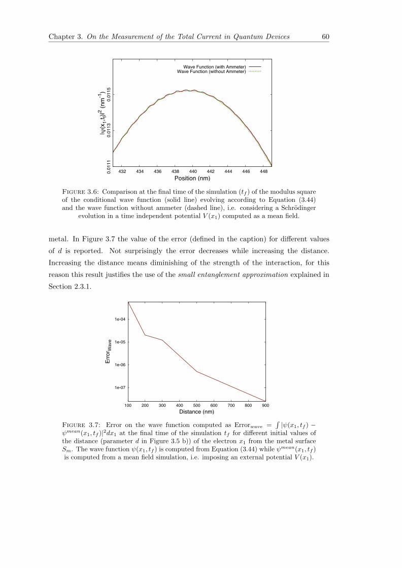
Chapter 3. On the Measurement of the Total Current in Quantum Devices 60
0.01
110.
0113
0.01
15
432 434 436 438 440 442 444 446 448
|s(x
1,t f)
|2 (nm
-1)
Position (nm)
Wave Function (with Ammeter)Wave Function (without Ammeter)
Figure 3.6: Comparison at the final time of the simulation (tf ) of the modulus squareof the conditional wave function (solid line) evolving according to Equation (3.44)and the wave function without ammeter (dashed line), i.e. considering a Schrodinger
evolution in a time independent potential V (x1) computed as a mean field.
metal. In Figure 3.7 the value of the error (defined in the caption) for different values
of d is reported. Not surprisingly the error decreases while increasing the distance.
Increasing the distance means diminishing of the strength of the interaction, for this
reason this result justifies the use of the small entanglement approximation explained in
Section 2.3.1.
1e-07
1e-06
1e-05
1e-04
100 200 300 400 500 600 700 800 900
Erro
r Wav
e
Distance (nm)
Figure 3.7: Error on the wave function computed as Errorwave =∫|ψ(x1, tf ) −
ψmean(x1, tf )|2dx1 at the final time of the simulation tf for different initial values ofthe distance (parameter d in Figure 3.5 b)) of the electron x1 from the metal surfaceSm. The wave function ψ(x1, tf ) is computed from Equation (3.44) while ψmean(x1, tf )is computed from a mean field simulation, i.e. imposing an external potential V (x1).

Chapter 3. On the Measurement of the Total Current in Quantum Devices 61
3.2.4 Computations of the Total Current
The instantaneous current measured in the surface SL when considering the contribution
of all the electrons in the metal or when considering only the electron in the device active
region, i.e. without including the apparatus, differs considerably as shown in Figure 3.8.
-0.15
-0.1
-0.05
0
0.05
0.1
0.15
0.2
0 0.02 0.04 0.06 0.08 0.1 0.12 0.14 0.16 0.18 0.2
Cur
rent
(µA)
Time (ps)
Instantaneous Current (without Ammeter)Instantaneous Current (with Ammeter)
Figure 3.8: Value of the total current. With solid line is reported the instantaneousvalue of the total current calculated from Equation (3.45) (with ammeter) and withdashed lines obtained from a mean field simulation for particle x1 alone (without am-
meter).
The large fluctuations in the current reported in Figure 3.8 means an additional source
of noise due to the interaction of the electrons in the metal with the particle x1 in the
active region of the device. Considering this additional source of noise, whose origin is
the quantum back-action, is mandatory to get accurate THz predictions.
0
20
40
60
80
100
120
140
160
180
0.7 0.8 0.9 1 1.1 1.2 1.5 1.7 2
Rel
ativ
e C
urre
nt E
rror (
%)
Frequency (THz)
d = 100 nmd = 300 nmd = 500 nmd = 900 nm
Figure 3.9: Relative error for the total current as a function of frequency (f = 1/T )calculated as |IT (t) − I
x1
T (t)|/|Ix1
T (t)|. The IT (t) is the mean temporal current at theconsidered frequency taken from Equation (3.45) (with ammeter) and I
x1
T (t) is meantemporal total current obtained from a mean field simulation (without ammeter). The
different curves represent different values of the parameter d.

Chapter 3. On the Measurement of the Total Current in Quantum Devices 62
In Figure 3.9 the relative error (defined in the caption) as a function of the frequency
(f = 1/T ) is reported. It can be seen that the error decrease for small frequencies (i.e.
for large intervals T for time-averaging). Additionally, it can be seen in Figure 3.9 that
when the distance d is increased (different curves in the plot), the relative error in the
measured total current grows.
3.2.5 Weak Measurement
From the previous results, it can be clearly seen that when the information of the
measured total current is very noisy, the quantum system is only slightly perturbed,
and vice versa. This fact is completely in agreement with the fundamental rules of
quantum measurement: if one looks for precise information, one has to pay the price of
perturbing the system significantly (the so-called collapse of the wave function or strong
measurement [82]). On the other hand if one does not require such a precise information
(for the instantaneous value of the total current seen in Figure 3.8) one can leave the wave
function of the system almost unaltered (known in literature as weak measurement). At
this point one can wonder if repeating many times the same (numerical) experiment
the mean value of the (weak) measured total current computed from Equation (3.45) is
equal to the value obtained without considering the ammeter.
0
0.02
0.04
0.06
0.08
0.1
-0.1 -0.05 0 0.05 0.1
Prob
abilit
y To
tal C
urre
nt
Total Current (µA)
Figure 3.10: Red solid line probability distribution of the measured total current fromEquation (3.45) in a time interval T = 0.2 ps of the simulation from 39000 experiments.
Green dashed line mean value obtained form a mean field simulation.
In Figure 3.10, the mean value of the probability distribution of the total current (with
ammeter) corresponds exactly to the mean value of the total current of the system
without ammeter. Let us mention that this mean value is exactly what one would
have found by performing several ideal strong measurement on the quantum system and
averaging them.

Chapter 3. On the Measurement of the Total Current in Quantum Devices 63
Next Chapter will be devoted to a further inspection of the weak measurement just found:
it will be detailed a procedure to compute the weak value of the Bohmian velocity in
mesoscopic systems through two measurements of the total current, one weak and one
strong. Numerical experiments will support the proposed experiments.


Chapter 4
Weak Measurement of Bohmian
Velocity in Mesoscopic Systems
The present Chapter is devoted to a proposal for weak measuring the Bohmian velocity
in a mesoscopic system. In the last years an increasing attention has been posed on
the utility of weak measurements [1] for exploiting new and fascinating quantum phe-
nomena. A weak measurement implies that the measuring apparatus provides a small
perturbation on the measured system and that the output result has a large uncertainty.
Although quantum mechanics forbids to measure simultaneously the position and the
momentum of a quantum particle in a single experiment, weak measurements realized
on a large set of identically prepared systems provide well-defined values of momentum
and position of the quantum system. These type of measurements open new paths for
wave function [13] or trajectories [45] (which reveal to be exactly the ones predicted
by Bohmian mechanics [29, 34]) reconstructions. Up to now, all such experiments are
done with (relativistic) photons and, unfortunately, a procedure to perform weak mea-
surements for (non-relativistic) electrons in solid-state devices does not exist. For this
reason, this Chapter is devoted to investigate numerically the feasibility of an experi-
ment for weak measuring the Bohmian velocity from the (high-frequency) displacement
current measured by an ammeter in a solid-state electronic device. The methodology
described in Section 3.2 and the results obtained there will be used in the present Chap-
ter.
65

Chapter 4. Weak Measurement of Bohmian Velocity 66
4.1 Weak Measurement of Bohmian Velocity from the To-
tal Electrical Current
Hereafter an introduction to the theory of weak measurement will be provided in Sec-
tion 4.1.1. Then in Section 4.1.2 several important results for the present thesis will be
derived. In Section 4.1.2.1 a formula connecting the measurement of the displacement
current in a large surface to the momentum of a particle in the active region of the
device will be obtained and in Section 4.1.2.2 it will be justified that this measurement
is weak. In Section 4.1.2.3 a formula connecting the measurement of the total current
in a small surface to the position of the particle will be achieved. These results will be
used in Section 4.2 and Section 4.3 to detail a proposed experiment to reconstruct the
Bohmian trajectories in a solid state system.
4.1.1 Theory of Weak Measurement
In Section 3.2.5 it has been argued that the measurement scheme proposed in Section 3.2
is weak. Hereafter it will be detailed the precise mathematical meaning resuming the
main feature of what is known as weak measurement.
In 1988 Aharonov, Albert and Vaidman [1] proposed the idea of generalizing the usual
projective measurement. Imagine one wants to measure the position of a particle, the
associated operator being x, the eigenstates of this operator are a continuum with the
carnality of <. One can introduces a general notion of operator, the so called POVM
(Positive Operator Value Measure), able to embodies the intrinsic uncertainty in a mea-
surement apparatus. For example, it can be chosen the following Gaussian measurement
Kraus operator [46]:
A =
(1√πσa
) 12∫dxe
− (x−xa)2
2σ2a Px, (4.1)
where σa is the width of the gaussian, Px = |x〉〈x| is the projection operator and xa
is the value registered by the measuring apparatus. The operator in Equation (4.1)
changes the system initial wave function ψ0(x) as follows:
ψf (x) = N Aψ0(x) = N(
1√πσa
) 12
e− (x−xa)2
2σ2a ψ0(x), (4.2)

Chapter 4. Weak Measurement of Bohmian Velocity 67
where N is the normalization constant.
Thus the wave function after the measurement ψf (x) will be a Gaussian-weighted sum
of projection of the initial wave function ψ0(x) onto the eigenstates of x. The operator
in Equation (4.1) is quite general, it is interesting to study two limiting cases depending
on the width σa of the Gaussian. Calling σf the width of the wave function (in the
position representation), if σa � σf the operator in Equation (4.1) is a quasi-projection
operator and it is referred to a strong operator, otherwise if σa � σf the operator in
Equation (4.1) is referred to a weak operator.
Defining σs ≡ σa and xs ≡ xa, a strong measurement of the position can be envisioned
as reported in Figure 4.1:
• In Figure 4.1 a) it is shown the wave function of the system at time t = 0 isolated,
evolving unitarily according to the Schrodinger equation.
• In Figure 4.1 b) it is shown the strong operator acting on the system wave function.
The strong operator is depicted with a green dashed zone, the width of the gaussian
is σs and is centered around position xs.
• In Figure 4.1 c) it is shown the wave function of the system after the application
of the Gaussian measurement Kraus operator. It can be seen that what survives
is only the part of the wave function that was, at time t = 0, around the measured
position xs.
The operator defined in Equation (4.1), with σa � σf , provides a notion of strong
measurement near to what it is a real measurement apparatus. Looking at Equation (4.2)
one deduces that the wave function ψf (x) is almost collapsed around position xs (see
Figure 4.2 c)).
The width of the gaussian, σa, defines the precision of the instrument or in other words
the reliability of the information extracted from the system by the measurement process.
The idea of weak measurement is then to relax and decrease the disturbance of the
system undergoing a measurement process. The price to be paid is that the amount of
information provided by the measuring apparatus in a single measurement is not reliable.
As stated before, the relevant condition is that σa � σf . Defining σw ≡ σa and xw ≡ xa,a weak measurement of the position can be envisioned as reported in Figure 4.2:
• In Figure 4.2 a) it is shown the wave function of the system at time t = 0 isolated,
evolving unitarily according to the Schrodinger equation.

Chapter 4. Weak Measurement of Bohmian Velocity 68
Initial Wave Function Initial Wave FunctionStrong Operator
Wave Function after Strong Measurement
x
x
x
⎮𝜓⎮²
⎮𝜓⎮²
⎮𝜓⎮²
a) b)
c)
xs
xs
Figure 4.1: Schematic representation of a strong measurement process. a) At theinitial time t = 0 the wave function (red solid line) of the system is not interacting witha measuring apparatus. b) The strong operator (green line) acts on the wave function ofthe system. c) After the interaction, the wave function of the system collapses around
the measured value xs.
• In Figure 4.2 b) it is shown the weak operator acting on the system wave function.
The weak operator is depicted with a yellow dashed zone, the width of the gaussian
(that does not enter entirely in the figure) is σw and is centered around position
xw
• In Figure 4.2 c) it is shown the wave function of the system after the application of
the weak Gaussian measurement Kraus operator. It can be seen that the function
is almost equal to the initial one in Figure 4.2 a). It is worthwhile to notice that
the wave function of the system does not keep track of the value xw measured by
the apparatus.
An important property of weak measurement is that the mean value of a weak mea-
surement (over an ensemble of identically prepared experiments) is exactly equal to the
mean value of the quantity measured. Calling |ψ〉 the initial wave function one has:

Chapter 4. Weak Measurement of Bohmian Velocity 69
Initial Wave Function
x
x
x
⎮𝜓⎮²
⎮𝜓⎮²
⎮𝜓⎮²
a) b)
c)
Initial Wave Function
Weak Operator
Wave Function after Weak Measurement
xw
Figure 4.2: Schematic representation of a weak measurement process. a) At the initialtime t = 0 the wave function (red solid line) of the system is not interacting with ameasuring apparatus. b) The weak operator (yellow line) acts on the wave function ofthe system. c) After the interaction, the wave function of the system remains almost
unaltered.
〈xw〉 =1√πσa
∫xwP(xw)dxw =
=1√πσa
∫xw〈ψ|A†A|ψ〉dxw =
=1√πσa
∫ ∫xwe
− (x−xw)2
σ2w 〈ψ|x〉〈x|ψ〉dxdxw =
=
∫x|ψ(x, 0)|2dx = 〈x〉. (4.3)
It is possible to summarize the main feature of a weak measurement: it provides a small
perturbation of the wave function (see Equation (4.2)), a single experiment does not
provide any reliable information about the measured system (see Figure 4.2) but the
mean value (over an ensemble of identically prepared experiments) is the same of the
usual strong measurement (see Equation (4.3)).

Chapter 4. Weak Measurement of Bohmian Velocity 70
4.1.2 On the Total Current Measured on Different Metallic Surfaces
In this Section it is analyzed the result found in Equation (3.32) in two different regimes:
Firstly, it will be analyzed for a large metallic surface and after for a small metallic
surface. The precise definition of “large” and “small” will be explained in details.
4.1.2.1 Total Current on an Large Surface S
It is interesting first of all to evaluate Equation (3.32) in the situation in which S �(xD−x)2: this means that the maximum distance (squared) that an electron in a device
can reach form the surface is much smaller than the surface itself. In order to work
out an approximate form for Equation (3.32) in this regime it can be considered the
following change of variable χ = (xD−x), and it can be assumed for simplicity that the
electron is located on the left of the surface (i.e. x < xD → χ > 0) then:
Φ(Ex(χ)) =q
πεtan−1
S
4χ√χ2 + S
2
=q
πεtan−1
S
4χ2√
1 + S2χ2
. (4.4)
Then, calling ξ2 = 2χ2
S , Equation (4.4) becomes
Φ(ξ) =q
πεtan−1
(1
2√ξ2(1 + ξ2)
), (4.5)
such that the condition S � χ2 becomes equivalent to ξ � 1. So Equation (4.5) becomes
simply:
Φ(ξ)ξ2�1 =q
πεtan−1
(1
2√ξ2
). (4.6)
Remembering that tan−1(αξ) + tan−1( 1αξ ) = π
2 for ξ > 0 (this implies that the electron
is on the left of the surface) then one has:
Φ(ξ) =q
πε
[π2− tan−1 (2ξ)
]. (4.7)
In Equation (4.7) the term tan−1(2ξ) can be expanded obtaining:

Chapter 4. Weak Measurement of Bohmian Velocity 71
Φ(ξ) =q
πε
[π
2− 2ξ +
(2ξ)3
3− ...
]. (4.8)
This last expression, Equation (4.8), can be truncated at first order of ξ. Thus recalling
the original variables one arrives at:
Φ(Ex(x;xD)) =q
πε
[π
2− 2
√2
S(xD − x)
]∝ x. (4.9)
Equation (4.9) is an important results, it demonstrates that the flux of the electric field
generated by a particle in a very large surface is proportional to the position of the
electron.
Now it can be discussed the general problem considered here, i.e. derive a microscopic
analysis of the measurement of the total electrical current in a large metallic surface.
In order to do that one has to “enlarge” the system considering also all the electrons
composing the metallic surface, as done in Section 3.2.
Without assuming nothing about the dynamics of the the electrons in the metal one can
say that they contribute as the electron in the device to the flux of the total electric field
as described by Equation (4.9) by superposition principle. One obtains, suppressing the
dependence on xD and making reference to the position of the electron in the device as
X1, the following expression:
Φ(Ex(X1, X2, X3, ..., XN )) = αX1 + α
N∑j=2
Xj , (4.10)
where the actual Bohmian positions of the particles Xi have been used and α is a suitable
constant. In expression Equation (4.10) one can clearly see that the total electric flux
is due to a contribution from the electron in the system ∝ X1 and another due to all
the other electrons in the metal. The latter is the additional source of noise found in
Section 3.2.
So far, it has been considered that the electron in the active region of the device is not
crossing the surface and therefore one gets that the total electric current is due only to
the displacement current contribution. So the total current becomes:
ITSlarge∝ dΦ(E)
dt=
d
dt
αX1(t) + αN∑j=2
Xj(t)
∝ vx1 +
N∑j=2
vxj , (4.11)
Chapter 4. Weak Measurement of Bohmian Velocity 72
where vxi∀i is the x-component of the Bohmian velocity of the i-particle. It will be
demonstrated in Section 4.3 numerically that the term∑N
j=2〈vxj 〉 ≈ const. over an
ensemble of repeated experiment. This result is not surprising because it has been
already achieved in Section 3.2 that the electrons in the metals act as an additional
source of noise not changing the mean value. So, it is possible to write:
〈IT 〉Slarge∝ 〈px1〉. (4.12)
Equation (4.12) shows that the mean value of the total electrical current in a large
metallic surface is proportional to the mean value of the momentum (x-component, i.e.
the component perpendicular to the surface) of the quantum particle in the device.
4.1.2.2 Is the Measurement on a Large Surface a Weak Measurement?
In the previous Section it has been demonstrated that the measurement of the total
current in a large surface is proportional to the (Bohmian) momentum of the particle in
the active region of the device. Here it is addressed the question: is this measurement
weak? As seen in Section 4.1.2.1 a weak measurement requires that: the measurement
does not perturb (too much) the wave function, that the information extracted from a
single experiment is not reliable and that the mean value corresponds exactly to the mean
value of a strong measurement of the same quantity. Now, the simulations performed in
Chapter 3 turns out to be very useful. There, it was simulated an electron in the active
region of a device interacting with others electron in a surface and the total current was
measured on a large surface S, exactly the condition considered here.
In Section 3.2.3 and Section 3.2.4 it has been shown that if one wants precise information
about the measured system, the perturbation of the wave function is increased, and vice
versa (see Figure 3.7 and Figure 3.9 respectively). It has been also proven in Section 3.2.5
that the mean value obtain from the simulations with ammeter is equal to the mean
value without ammeter (of the system alone), as clearly shown in Figure 3.10. So, all
the conditions exposed at the beginning of this Section are satisfied, thus configuring the
measurement of the total current in a large surface as a weak measurement. Thus adding
the result obtained in Equation (4.12), the weak measurement of the total current can
be written in the language of Gaussian measurement Kraus operator as:
Iw = Cw
∫dpe−
(p−pw)2
2σw |p〉〈p|, (4.13)

Chapter 4. Weak Measurement of Bohmian Velocity 73
where p is the momentum (x-component) of the particle in the device and Cw is suitable
constant (for more details see Appendix C).
Now, it will be discussed how the width σw of the Gaussian measurement Kraus operator
changes with the frequency. It has been seen that depending on the frequency the
information about the measured total current changes (see Figure 3.9). In Figure 4.3 it
is reported how σw varies with the frequency of the measurement. It can be seen that
lowering the frequency yelds more precise information about the system (the width of
the gaussian decreases). In this sense the proposed experiment works in a regime where
the total current is measured at High-Frequency.
0
0.02
0.04
0.06
0.08
0.1
0.12
0.14
0.16
-0.15 -0.1 -0.05 0 0.05 0.1
Prob
abilit
y To
tal C
urre
nt
Total Current ( A)!
Figure 4.3: Blue dashed line probability distribution of the measured total currentat a frequency of f = 5 THz. Red solid line probability distribution of the measured
total current at f = 50 GHz.
4.1.2.3 Total Current on a Small Surface S
Now, it is interesting to consider the opposite limit in which the surface S where the
measurement is performed is very small compared to the distance of the electron from
the surface χ = xD − x. Specifically one has to consider Equation (4.4) in the limit
in which S � χ assuming as before that the electron is on the left of the surface, i.e.
χ > 0. Making the following change of variable ξ = S2χ2 the previous condition becomes
equivalent to study the condition ξ � 1 for the function
Φ(Ex(ξ)) =q
πεtan−1
(ξ
2√
1 + ξ
), (4.14)
it can be easily seen that the first order expansion of the last expression is:

Chapter 4. Weak Measurement of Bohmian Velocity 74
Φ(Ex(x;xD)) =q
4πε
S
(xD − x)2for x < xD. (4.15)
The physical interpretation of this term is quite natural: the contribution of a particle
to the total flux measured in a small surface is only relevant when the particle is “near”
the surface. This means that the the contribution is relevant when the electron cross
the surface. For this reason it has been pointed out that the function (3.32) has a
discontinuity in the point x = xD of the first kind. In order to ensure continuity one
has to add to the total flux of the electric field the particle contribution of the current.
This is simply proportional to qΘ(x− xD) where Θ(x) is the Heaviside function. Then
with the add of this contribution one has that, in the limit of small surface, the particle
contribution is the main contribution, when an electron crosses the surface. Extending
this result to quantum mechanics is trivial and gives for the total current measured on
the small surface:
〈IT 〉Ssmall∝ 〈δ(x1 − xD)〉 =
∫dx1ψ
∗(x1, t)δ(x1 − xD)ψ(x1, t) (4.16)
where ψ(x1, t) is the wave function of the electron in the device. Equation (4.16) ex-
plains the obvious relation that measuring the total current in a small surface provides
information whether or not the particle is passed through the surface or not. It is im-
portant to mention that in this case one does not need to include all the others electrons
in the metal because one can see that the first interaction that the electron in the device
suffers is already strong. In principle a treatment including the rest of the electrons of
the system can be provided but in this case the result obtained does not change; in fact
the electron in the device contributes to the total current only when pass through the
small surface and then when the interaction with all the others electrons in the metal is
strong (the distance is very small).
Thus it is possible to write the measurement of the total current in a small surface S in
the language of the Gaussian measurement Kraus operator as:
Is = Cs
∫dxe−
(x−xs)2
2σs |x〉〈x|, (4.17)
with σs satisfying the condition exposed in Section 4.1.1 and Cs a suitable constant (see
Appendix C).

Chapter 4. Weak Measurement of Bohmian Velocity 75
4.2 Geometry of the Proposed Experiment
Once the theory of weak measurement has been developed and the results in Sections
4.1.2.1, 4.1.2.2 and 4.1.2.3 have been achieved, it is possible to propose a specific device
geometry for measuring the Bohmian velocity in mesoscopic systems.
Figure 4.4: Schematic representation of a three terminal device to measure theBohmian velocity in a mesoscopic system.
In Figure 4.4 it is reported a schematic representation of the three terminal device pro-
posed here. There are two metallic surfaces working as sensing electrodes. The surface
on the right Sw satisfies the relation Sw � L2x, thus the total current measured by
the w-ammeter follows the relation given by Equation (4.12) found in Section 4.1.2.1.
Therefore, the w-ammeter would measure a quantity proportional to the momentum of
the particle in the active region of the device (see Equation (4.13)). At the left side of
Figure 4.4, it can be seen that a similar metallic surface, Sg, is depicted connected to
the g-ammeter. From this surface a small part of it, Ss, is electrically isolated and con-
nected to a different ammeter than g, called s-ammeter. This third s-ammeter, because
Ss � L2x, would provide a measurement of the total current that is proportional to the
position of the particle in the active region of the device (see Equation (4.16) in Sec-
tion 4.1.2.3). In order to ensure that the two different conditions used in Section 4.1.2.1
and Section 4.1.2.3 are satisfied it has been considered the square of the length Lx as the
maximum distance the particle can reach from the surface. Now it is possible to work
out the exact procedure for measuring the Bohmian velocity, the w-ammeter measures
weakly the momentum of the particle, these values will be post-selected by positions
measurement performed by the s-ammeter.

Chapter 4. Weak Measurement of Bohmian Velocity 76
4.2.1 Derivation of Bohmian Velocity Weak Value
With the operators defined in Section 4.1.1 it is possible to derive mathematically how
the Bohmian velocity can be obtained from a weak measurement procedure with post
selection for the device geometry just exposed. The reader can found analogous math-
ematical developments in Refs. [34, 80, 83]. One is interest in the quantity E[pw|xs],i.e. the ensemble average values of the (weak measured) momentum pw conditioned to
the fact that (strong) position xs is effectively measured. Using standard probabilities
formulas, this quantity can be simply computed as:
E[pw|xs] =
∫dpwpwP(pw ∩ xs)
P(xs), (4.18)
where P(pw ∩xs) is the joint probability of two sequential measurement pw and xs, and
P(xs) is the probability of xs. The quantity P(xs) is computed as follows:
P(xs) =
∫dpwP(pw ∩ xs) =
∫dpw〈ψ|I†wU †τ I†s IsUτ Iw|ψ〉, (4.19)
where |ψ〉 ≡ |ψ0〉 is the initial wave function, Uτ the unitary evolution operator and
the probability P is computed as 〈ψ|...|ψ〉 using Born’s rule. The operators Iw/s are
defined in Equation (4.13) and Equation (4.17) respectively. Therefore Equation (4.19)
becomes:
P(xs) =
∫ ∫dp′dp′′e
− (p′−p′′)2
4σ2w 〈ψ|p′〉〈p′|U †τ I†s IsUτ |p′′〉〈p′′|ψ〉, (4.20)
with the assumption e− (p′−p′′)2
4σ2w ≈ 1, that is equivalent to σw → ∞, the last expression
becomes:
P(xs) = 〈ψ|U †τ I†s IsUτ |ψ〉 = |ψ(xs, τ)|2. (4.21)
The last step needed to obtain the Bohmian velocity from Equation (4.18) is to calculate
its numerator:

Chapter 4. Weak Measurement of Bohmian Velocity 77
∫dpwpwP(pw ∩ xs)=
∫∫dp′dp′′
(p′ + p′′
2
)e− (p′−p′′)2
4σ2w 〈ψ|p′〉〈p′|U †τ I†s IsUτ |p′′〉〈p′′|ψ〉.(4.22)
Using again the condition σw →∞ and the definition∫p|p〉〈p| = p one gets
∫dpwpwP(pw ∩ xs) = Re
(〈ψ|U †τ I†s IsUτ p|ψ〉
)= mJ(xs, τ) (4.23)
where Re(...) denotes the real part and J(xs, τ) is the usual probability current. Hence,
one gets the conclusion:
E[pw|xs]m
=J(xs, τ)
|ψ(xs, τ)|2≡ v(xs, τ), (4.24)
where v(xs, τ) is exactly Bohmian velocity. A detailed derivation of the result found
in Equation (4.24) is reported in Appendix C, in which is also specified the condition
σw →∞ in relation to σs.
Next Section is devoted to show a numerical experiment with the set-up reported in Fig-
ure 4.4 in which is possible to obtain the Bohmian velocity through a weak measurement
of the momentum post-selected with strong measurement of position.
4.3 Numerical Experiments
The simulations reported in this Section are done following of what shown in Section 3.2.
In particular the measurement of post selection of position is obtained without explicitly
simulating the s-ammeter, but it is obtained directly from the Bohmian position of the
electron in the active region of the device. In fact, a strong measurement of the position
reveals nothing else that the position of the Bohmian particle [35]. The surface where
the weak measurement is performed is Sw ≈ 10−11 m2 while the length of the device
is Lx = 2, 8 · 10−7 m. The electron in the metal surface are simulated as described in
Section 3.2.2.1.
In Figure 4.5 it is reported the velocity v(xs, t) obtained from an ensemble of 55000
identically prepared experiments. In particular as initial wave function ψ(x1, 0) has

Chapter 4. Weak Measurement of Bohmian Velocity 78
Cur
rent
(nA
)
Position (nm)
With ammeterWithout ammeter
Figure 4.5: Red points (with error) Bohmian velocity in position xs at time t =300 fs, obtained from an ensemble of 55000 experiments with the inclusion of theelectrons in the metal surface (with ammeter) as reported in Section 3.2. The error iscalculated from the standard deviation of the ensemble at time t and position xs dividedby the square root of trajectories passing through position xs at time t. Green solidline Bohmian velocity in position xs obtained from the same set of simulations withoutconsidering the electrons in the metal surface (without ammeter). In the numericalexperiment reported in this Section the total current is measured at a frequency f =
5 · 1013 Hz.
been chosen a superposition of two gaussian wave packets which have the central position
spatially separated of 50 nm (as it can be seen at the initial time in Figure 4.6). Each
gaussian wave packet has the same dispersion of 3 nm and the same energy of 0.0905 eV .
The velocity field exhibits the typical maximum and minima of the interference pattern.
In Figure 4.6 the modulus square of the wave function in function of time is reported.
Figure 4.6: Density plot of the modulus squared of the wave function in function oftime. It can be easily seen how the two initial wave packets spread forming the usualinterference pattern. This figure has been obtained only from the trajectories without
ammeter used for simulating the experiments.
In Figure 4.7 b) are reported the trajectories reconstructed with the procedure detailed
in Section 4.2.1 from the 55000 simulations. In Figure 4.7 a) are reported the trajectories

Chapter 4. Weak Measurement of Bohmian Velocity 79
obtained without considering the electrons in the metal surface.
Elec
tron
Posi
tion
(nm
)
Time (fs)Time (fs)
Elec
tron
Posi
tion
(nm
) a) b)
Figure 4.7: Bohmian trajectories obtained from simulation without ammeter a) andwith ammeter b).
It is important to mention that the trajectories reconstructed in Figure 4.7 are obtained
calculating the proportionality constant in Equation (4.12) not using the constant α
found in Equation (4.10) but directly from the numerical simulations without ammeter.
One can see in Figure 4.7 that there is an excellent agreement between the trajectories
obtained from the weak measurement procedure and the exact ones.
Elec
tron
Posi
tion
(nm
)
Time (fs)
Elec
tron
Posi
tion
(nm
)
Time (fs)
Elec
tron
Posi
tion
(nm
)
Time (fs)
Wave function
Bohmian trajectoriesWave function +
Bohmian trajectoriesa) b)
c)
Figure 4.8: a) Same wave function reported in Figure 4.6. b) Trajectories obtainform the weak measurement procedure described in the text. c) Wave function andBohmian trajectories in the same plot. As explained in the text, Bohmian trajectoriesare more dense near the maximum of the interference pattern while are less dense near
the minimums.

Chapter 4. Weak Measurement of Bohmian Velocity 80
As a final result, in Figure 4.8 is reported the comparison of the trajectories obtained
from the procedure described in Section 4.2.1 with the same wave function depicted in
Figure 4.6. It can be seen that, as expected from Bohmian Mechanics, the trajectories are
more dense near the maximum and are less dense near the minimum of the interference
pattern of the wave function.

Chapter 5
Time-Dependent Problems in
Quantum Transport
The present Chapter is devoted to two problems in quantum transport. The two prob-
lems are neither strictly related to each other nor to the foregoing Chapter, but both
rely on the techniques developed so far. In Section 5.1, inspired by a recent experiment
[14], two particles scattering probabilities for a HOM-type (Hong-Ou-Mandel) experi-
ment are analyzed. The time-dependent nature of this problem is addressed here, by
considering as initial states localized wave packets instead of plane waves: this leads to
surprising and interesting results. In Section 5.2, the time-dependent nature of the evo-
lution of the conditional wave function is used in understanding the origin of quantum
noise in mesoscopic system. As it will be seen, this analysis leads to a two-time measure
of a quantum system. It will be argued that quantum noise is easily understood and
computed within Bohmian Mechanics. All the discussion about the collapse done in
Chapter 2.1, and the numerical example studied in Section 3.1, will be used extensively,
as well as the numerical simulation techniques.
5.1 Detection at the Same Place of Two Simultaneously
Emitted Electrons
The present Section is inspired by a recent experiment [14] in which two initial electrons
wave packets (with opposite central momentums) are spatially localized at each side of
a barrier. Then, after impinging upon a tunneling barrier, each wave packet splits into
transmitted and reflected components. Contrarily to what is claimed in the literature,
it is shown that the probability of detecting two (identically injected) electrons at the
81

Chapter 5. Time-Dependent Problems in Quantum Transport 82
same side of the barrier is different from zero in very common (single or double barrier)
scenarios and for any type of (normalizable) state. For some particular resonant energies
and wave packets, the transmitted and reflected components become orthogonal and the
mentioned probabilities reproduce those values associated to distinguishable particles.
These unexpected non-zero probabilities are still present when Coulomb interaction or
non-symmetrical potential are considered. On the other hand, for initial wave packets
close to Hamiltonian eigenstates, the usual zero probability for electrons at the same
side of the barrier found in the literature is recovered. The far-reaching consequences
of these non-zero probabilities in the evaluation of quantum noise in some scenarios is
briefly addressed.
The present Section is divided as follows: Hereafter a brief introduction of the problem
and the main motivations are given. In Section 5.1.1 the general expressions for the prob-
abilities of detecting two electrons are defined. In Section 5.1.2, numerical test for typical
tunneling scenarios with symmetric (Section 5.1.2.1) or non-symmetric (Section 5.1.2.2)
potentials are presented. Among others, to go beyond the Fermi liquid picture of (non-
interacting) electrons, a subsection (Section 5.1.2.3) is dedicated to investigate the effect
of including Coulomb interaction among the electrons in a two-particle system. Addi-
tionally, a single barrier potential, which is a physical system closer to the experiment
mentioned above, is also analyzed numerically (Section 5.1.2.4). In all the four scenarios
discussed in Section 5.1.2 clear non-zero probabilities of detecting two electrons at the
same side of the barrier are obtained. Section 5.1.3 is dedicated to summarize the main
results achieved in the present Section and to indicate further consequences of the results
obtained.
The ultimate reason why the quantum theory gives rise to a host of puzzling and fas-
cinating phenomena is because many-particle quantum systems are defined in a high-
dimensional and abstract configuration space. For example, in a system of identical
particles, only those wave functions whose probability density in the configuration space
remains unchanged under permutations of particles are acceptable. When this happens,
it is said that the system has exchange interaction. One consequence of the exchange
interaction is the Pauli repulsion, that forces electrons to avoid common positions.
In systems with stationary probability distributions, the effect of the exchange interac-
tion in the scattering probability needs to be discussed only once. On the other hand,
one can envision a richer phenomenology in scenarios with time-dependent probability
distributions when, for example, electrons share common positions at the final time, but

Chapter 5. Time-Dependent Problems in Quantum Transport 83
not at the initial one. A typical scenario for discussing exchange and tunneling phenom-
ena with time-dependent probability distributions is shown in the scheme of Figure 5.1.
Two electrons with the same energy and opposite momentum are injected simultaneously
from two different sources. During the interaction with a tunneling barrier, each wave
packet splits into a transmitted and a reflected part. At the final time, transmitted and
reflected components of different electrons share common positions and the effect of the
exchange interaction becomes relevant. This typical scenario in the study of quantum
transport in mesoscopic systems shown in Figure 5.1 can also be interpreted as a type
of two-particle interference Hong-Ou-Mandel (HOM) experiment developed some time
ago for photons [43].
Within the (Landau) Fermi liquid theory [47–49], these type of experiments are tradition-
ally analyzed by describing the (quasi-particle) electrons as mono-energetic scattering
states [16, 17]. The creation and annihilation operators in the second quantization for-
malism provide a very elegant and powerful formalism to include exchange interaction
into tunneling problems. The (anti-symmetrical) initial state with one electron at each
side of the barrier is defined by |Ψ〉 = a†La†R|0〉. The scattering theory for mono-energetic
states predicts that the probability of finding one electron on the left and one electron
on the right of the barrier is:
PSLR = |〈0|bLbRa†La†R|0〉|
2 = 1, (5.1)
where the upperindex S indicates scattering formalism. Equivalently, the probability of
finding both electrons on the left is:
PSLL = |〈0|bLbLa†La†R|0〉|
2 = 0 (5.2)
and both electrons on the right is:
PSRR = |〈0|bRbRa†La†R|0〉|
2 = 0. (5.3)

Chapter 5. Time-Dependent Problems in Quantum Transport 84
Explicit computations of these probabilities are written in Appendix D. The same scat-
tering formalism (with the proper commutations properties for the creation and annihila-
tion operators) has been also used to successfully analyze this type of HOM experiments
for photons [16–18, 78].
In principle, one can imaging two clear limits for the defined physical quasi-particle
states. The first limit is assuming that the (quasi-)electrons are described by point-like
states in real space (very narrow wave packets). This limit is obviously unphysical. The
other limit is describing (quasi-)electrons by point-like states in the momentum space
(infinitely space extended wave packets). In fact, this second limit has been demon-
strated to be very successful in the literature. The celebrated scattering probabilities
presented in Equation (5.1), Equation (5.2) and Equation (5.3) fit within this second
limit. However, it seems reasonable to expect that the quasi-particle state that better
captures the physics of the system described in Figure 5.1, is an initial state with some
type of localization: an intermediate state between a point-like state in real space and
point-like state in momentum space (probably, quite close to the typical point-like states
in momentum state, but not exactly identical to them). In fact, the concept of quasi-
particle wave packets was used by Kohn et al. [40] some years ago when analyzing the
effect of the physical borders on localized (not infinite) systems. Equivalently, the con-
cept of one-particle wave function that still captures many-body correlations has been
deduced by Oriols et al. [68] through the use of the conditional wave function.
With this motivation, the mentioned two-particle scattering probabilities are analyzed
using localized time-dependent wave packets as initial states. It is computed the proba-
bility of detecting two electrons at the same side of the barrier from the anti-symmetric
solution of the time-dependent Schrodinger equation in the configuration space.1 The
main result is that in many scenarios (double and single barrier) the probability of find-
ing two identically injected electrons at the same side of the barrier differs from zero
(contrarily to what is claimed in the literature for time-independent scattering eigen-
states, i.e. Equation (5.2) and Equation (5.3)). The main conclusions about these
non-zero probabilities are developed for arbitrary shapes of the wave packets. On the
other hand, typical Gaussian wave packets (including point-localized or fully-extended
mono-energetic states as two limiting cases) are used to test and illustrate these non-zero
probabilities with numerical results. These results are in agreement with the recent ex-
periment of Bocquillon et al. [14], where unexpected non-zero probabilities of detecting
1The only assumption is that this type of two-electron interference experiments can be perfectlyunderstood from non-relativistic quantum mechanics, as most of the electron problems in chemistry andsolid-state physics.

Chapter 5. Time-Dependent Problems in Quantum Transport 85
both electrons at the same side of the barriers were obtained. They used single-electron
sources in order to ensure that two spatially localized wave packets with disjoint support
were prepared at the initial time. In addition, non-zero probabilities were also found
when beams of electrons were used by Liu et al. in a similar experiment [56]. This sug-
gests that these non-zero probabilities are not due to experimental spurious effects,2 but
due to the fundamental wave packet nature of the electrons present in such experiments.
The study of the quantum transport by describing (quasi) electrons by wave packets
was initiated by Loudon [55] when he considered the effect of the initial overlapping
between two wave packets on the scattering probabilities (not after the interaction with
the barrier as considered in this work, as depicted in Figure 5.1). However, this type of
studied was mainly ignored in the literature.
!
!
!
! !
!!!!!!"#$!!"!%&'()*+%%,-!'(-!!#!%&'()*+%%,-!!!!!!!!"'$!!"!&,./,0%,-!'(-!!#!&,./,0%,-!
1(0+-,(%! 2,./,0%,-! 3&'()*+%%,-!345,)!6.!7'8,!5'09,%):!
!$!"%
&$&'%
&$&(%
!$!#% !$!"%
&$&'%
&$&(%
!$!#%
!!!!!!"-$!!"!%&'()*+%%,-!'(-!!#!&,./,0%,-!!!!!!!!"0$!!"!&,./,0%,-!'(-!!#!%&'()*+%%,-!
!$!"%
&$&'%
&$&(%
!$!#% !$!"%
&$&'%
&$&(%
!$!#%
!!;6)+%+6(!
<,%,0%6&)!
!!;6)+%+6(!
<,%,0%6&)!
Figure 5.1: Two identically injected wave packets from the left xa and from the rightxb of a scattering barrier. Solid regions represent the barrier region and shaded regionsrepresent the particle detectors. (a) and (b) each particle is detected on a different sideof the barrier at final time t1 when the interaction with the barrier has almost finished.
(c) and (d) both particles are detected on the same side of the barrier.
2“The noise is not completely suppressed, in part because of non-idealities in the beam splitter’sscattering matrix.”[56]. “The states are not perfectly identical as shown by the fact that the dip does notgo to zero.” [14].

Chapter 5. Time-Dependent Problems in Quantum Transport 86
5.1.1 Two-Particle Probabilities
Consider two particles injected from two different sources and impinging upon a tunnel-
ing barrier as indicated in Figure 5.1. In order to simplify the discussion, it is assumed
that electrons have identical spin orientations. Each one is individually defined in a
1D physical space. The two-particle quantum system can be defined by the (orbital)
wave function Φ ≡ Φ(x1, x2, t) in the 2D configuration space. Such wave function is the
solution of the many-particle (non-relativistic) Schrodinger equation:
i~∂Φ
∂t=
[− ~2
2m
∂2
∂x21
− ~2
2m
∂2
∂x22
+ V (x1, x2)
]Φ, (5.4)
where m is the electron (boson) masses and V (x1, x2) takes into account the two-particle
Coulomb interaction between the electrons and also the one-particle interaction between
one electron and a tunneling barrier. The exchange interaction is introduced in the shape
of the initial wave function Φ(x1, x2, t0). The anti-symmetrical/symmetrical (orbital)
many-particle wave function for Fermions/Bosons is:
Φ(x1, x2, t0) =φa(x1, t0)φb(x2, t0)∓ φa(x2, t0)φb(x1, t0)√
2. (5.5)
The above expression can be interpreted as the determinant/permanent of a 2×2 matrix
constructed from the one-particle wave function φa(x, t0) and φb(x, t0) [22]. Hereafter,
upper/lower signs correspond to (non-relativistic) massive Fermions/Bosons. Although
electrons (Fermions) are mainly analyzed, probabilities will be also computed for (mas-
sive) Bosons. The initial one-particle wave functions φa(x, t0) and φb(x, t0) in Equa-
tion (5.5) are completely general. The only relevant condition for φa(x, t0) is that its
modulus square is normalizable to unity and it is totally located at the left of the barrier
at time t = t0. Identical conditions for φb(x, t0) which is localized at the right. Addi-
tionally, according to the type of HOM experiment discussed here, both wave packets
have opposite (central) momentum so that they impinge upon the barrier after a while,
as depicted in Figure 5.1. By construction, the time evolution of Φ(x1, x2, t) using Equa-
tion (5.4) preserves the initial norm and the initial (anti)symmetry of the wave function.
It is possible to give an intuitive and simple argument of why it is reasonable to expect
non-zero probability for finding both electrons at the same side of the barrier. Pauli
principle forbids two fermions being at the same position with the same state [69–71].
However, a pertinent question appears: When is reasonable the assumption that the
reflected and transmitted states are exactly identical? Certainly, both transmitted and

Chapter 5. Time-Dependent Problems in Quantum Transport 87
reflected states are identical when only one state is available in the spatial region where
they coincide. This restriction on the available states is evident when the initial state
has a unique (well-defined) energy Ek, i.e. a mono-energetic state. Then, because of the
elastic nature of the interaction with the barrier (i.e. energy conservation), only one state
at the right of the barrier and one at the left with the same energy Ek (and the pertinent
momentum going outside from the barrier) are available at the final time. Nevertheless,
as stated previously, here it is required a superposition of mono-energetic eigenstates (i.e.
a wave packet) to describe an initial state with a spatially localized support outside of
the barrier region. Then, in principle, there is the possibility of different time-evolutions
for the transmitted and reflected components. In such time-dependent scenarios, one can
expect probabilities different from zero (as mentioned before) as indicated in Figure 5.1
c) and Figure 5.1 d). Notice the different shapes of the reflected and transmitted wave
packet in Figure 5.1.
Consider a particular time t1 large enough so that the interaction with the barrier is
almost finished, i.e. the probability presence inside the barrier region is negligible. Then,
using Born’s rule [22] in the 2D configuration space, {x1, x2}, the probability of detecting
one electron at each side of the barrier (on regions SLR or SRL of the configuration space
depicted in Figure 5.2 a)) at this time t = t1 is:
PLR =
∫SLR|Φ|2dx1dx2 +
∫SRL|Φ|2dx1dx2 = 2
∫SLR|Φ|2dx1dx2. (5.6)
Due to the exchange symmetry, the wave function on SLR is identical to that on SRL,
as seen in Figure 5.2 a). The two integral in the left hand side of Equation (5.6) are
exactly equal, so the total contribution of finding one electron at each side of the barrier
is twice one of the integrals. Equivalently, the probability of detecting the two electrons
at the left of the barrier (on the region SLL of the configuration space) is:
PLL =
∫SLL|Φ|2dx1dx2. (5.7)
Finally, the probability of two electrons at the right of the barrier (on the region SRR)
is:
PRR =
∫SRR|Φ|2dx1dx2. (5.8)

Chapter 5. Time-Dependent Problems in Quantum Transport 88
PLR, PLL and PRR are defined as two-particle probabilities. In Figure 5.2 a) the
probability presence of the initial two-particle state is plotted in the 2D configuration
space. According to Equation (5.5), the wave packet φa(x1, t0)φb(x2, t0) has its support
on SLR, while the wave packet φa(x2, t0)φb(x1, t0) on SRL. There is no initial probability
presence in the other regions. The first relevant issue seen on the regions SLL and SRRof Figure 5.2 b) is that PLL 6= 0 and PRR 6= 0. The reason of these non-zero probabilities
is explained in details in next Section. In general, it is important to notice that there
is no reason to expect that the probability of detecting two electrons at the left of the
barrier is equal to the probability of detecting them at the right, PRR 6= PLL as seen in
Figure 5.2 b).
Figure 5.2: a) Modulus square of the wave function Φ(x1, x2, t0) at the initial time t0in the configuration space {x1, x2}. With black solid line is represented the scatteringbarrier. Along the axes the single particle wave packet φa(x, t0) are reported (redsolid line), φb(x, t0) (green solid line) for both variables (x1 and x2). The dotted linevisualize how the anti-symmetrical wave function is constructed. The different regionsof configuration space SLL,SLR,SRL and SRR are explicitly indicated. b) Modulussquare of the wave function Φ(x1, x2, t1) at the final time t1 (such that the interactionwith the barrier is already accomplished). Along the axes φa(x, t1) (red solid line) andφb(x, t1) (green solid line) for both variables {x1, x2} are reported . With dashed dottedblue line the anti-symmetry line for Fermions is indicated. As asserted in the text the
probabilities PRR 6= PLL 6= 0.
To certify the unavoidable fundamental (not spurious) origin of the non-zero probabilities
for PLL and PRR, hereafter, the same idealized conditions used in Refs. [12, 16, 17, 78]
when they discuss the two-particle probabilities are considered. The two wave packets
φa(x, t0) and φb(x, t0) are taken as identical as possible. In particular, the following
three conditions are imposed:
• Condition (i): A separable potential V (x1, x2) in Equation (5.4) without Coulomb
interaction:
V (x1, x2) = VB(x1) + VB(x2), (5.9)

Chapter 5. Time-Dependent Problems in Quantum Transport 89
where VB(x) is the symmetrical potential energy of a tunneling barrier, i.e. VB(x) =
VB(−x), with x = 0 at the center of the barrier region. See Figure 5.3 a).
• Condition (ii): All parameters of the initial wave packet a and b are identical,
except for the initial central momentums which accomplishes kb = −ka and central
positions xb = −xa. See Figure 5.3 a).
• Condition (iii): Electrons are injected exactly at the same time.
Because of these conditions, as discussed in Appendix E, the two initial wave packets are
defined with (almost) identical parameters. In particular, one has ga(k) = gb(−k) where
ga(k) = 〈φa(x, t0)|ψk(x)〉 is the complex value that weights the superposition of the
scattering states to build the wave packet φa(x, t0). See Equation (E.4) in Appendix E.
An identical definition is given for gb(k).
Figure 5.3: a) Schematic representation of the initial wave packets in the physicalspace under the conditions (i), (ii) and (iii). With black solid line the double barrierstructure is depicted. With orange dashed line the Left-Right symmetry of the problemis depicted. With red solid line wave packet φa(x) centered in xa and with momentumka is depicted. With green dashed dotted line the wave packet φb(x) centered in xb =−xa and momentum kb = −ka is reported . b) Modulus square of the wave functionΦ(x1, x2, t1) at the final time t1 at the configuration points {x1, x2}. With dasheddotted blue line the anti-symmetry line for Fermions is indicated and with orange dashedlines the Left-Right symmetry for each degree of freedom (x1 and x2) is reported. Alongthe axes, the modulus square of the φa (red line) and φb (green line) wave functionsare plotted for each degree of freedom (x1 and x2). The upper indices r or t indicate
reflected or transmitted components, respectively.
Under these conditions, it is possible to anticipate the evolution of Φ(x1, x2, t) and
also the origin of the non-zero probabilities for arbitrary wave packets. The initial
(anti-symmetrical) wave function of two electrons Φ(x1, x2, 0) considered is defined by
Equation (5.5). Since the time-evolution of Schrodinger equation satisfies the superpo-
sition principle, it is possible to discuss the time-evolution of φa(x1, t0)φb(x2, t0) and

Chapter 5. Time-Dependent Problems in Quantum Transport 90
φa(x2, t0)φb(x1, t0) independently. Then, since the Hamiltonian is separable, the evolu-
tion of φa(x, t) and φb(x, t) can be computed from two simpler single particle Schrodinger
equations. At a time t = t1, after the interaction with the barrier, each wave packet
splits into two (non-overlapping) components:
φa(x, t1) = φra(x, t1) + φta(x, t1), (5.10)
φb(x, t1) = φrb(x, t1) + φtb(x, t1), (5.11)
where the upper indices r and t refer to the reflected and transmitted component of
each wave packet (φa and φb), respectively. Then, the two particle wave function in the
region of the configuration space SLL at t = t1 is:
Φ(x1, x2, t1)∣∣SLL
=φra(x1, t1)φtb(x2, t1)− φra(x2, t1)φtb(x1, t1)√
2. (5.12)
Notice that the region SLL was initially empty of probability, as seen in Figure 5.2
a). The initial wave packet φa(x1, t0) on SLR (which is identical to the one plotted in
Figure 5.2 a)) evolves into the part φra(x1, t1) on SLL in Figure 5.3 b). Equivalently,
the initial wave packet φb(x2, t0) in Figure 5.2 a) evolves into the part φtb(x2, t1) on SLLin Figure 5.3 b). Identical explanations for the presence of φtb(x1, t1) and φra(x2, t1) on
SLL. Clearly, since PLL in Equation (5.7) is computed from an integral of non-negative
real numbers, the requirement for obtaining the result PLL = 0 in Equation (5.12) is
that φra(x1, t1)φtb(x2, t1) = φra(x2, t1)φtb(x1, t1) at all positions {x1, x2} ∈ SLL.3 This last
condition can only be obtained when φtb(x, t1) = φra(x, t1) and φta(x, t1) = φrb(x, t1). On
the contrary, if the transmitted and reflected wave packet components differ, i.e. if the
time-evolution giving the transmitted component φta(x, t1) is different from φrb(x, t1),
then one gets Φ(x1, x2, t1) 6= 0, which implies PLL 6= 0. Analogous consideration can be
done for the configuration space region SRR.
After discussing the origin of the non-zero probabilities, here a technical question is
addressed that it will be tested later numerically. The conditions (i), (ii) and (iii) impose
an additional symmetry on the problem. Apart from the intrinsic anti-symmetry of the
wave function implicit in Equation (5.5), there is an additional Left-Right symmetry.
This means that, being x = 0 the center of the barrier region as depicted in Figure 5.3
a), the wave function under the separable Hamiltonians of Equation (5.9) has to satisfy
Φ(x1, x2, t) = −Φ(−x1,−x2, t) at all times. This additional symmetry implies that the
3By construction, only in the configuration space points {x1, x2} ∈ SLL such that x1 = x2 the wavefunction is always strictly zero (see anti-symmetry line in the Figure 5.3 b)).

Chapter 5. Time-Dependent Problems in Quantum Transport 91
probability of detecting two electrons on the left is exactly equal to detect them on
the right, i.e. PLL = PRR as depicted in Figure 5.3 b). However, in general, when
conditions (i), (ii) and (iii) are not satisfied, one has PLL 6= PRR as depicted in the
preceding Figure 5.2 b).
The exact values of PLR, PLL and PRR depend on the effective overlapping between
φta(x, t1) and φrb(x, t1). In Appendix E analytical calculations are developed for the range
of values that the probabilities Equation (5.6)-Equation (5.8) can take when conditions
(i), (ii) and (iii) are assumed. When reflected and transmitted wave packets are identical
as indicated in Equation (E.13), expressions (5.6)-(5.8) can be rewritten as:
PMLL = PMRR = RT ∓RT, (5.13)
PMLR = (R± T )2, (5.14)
which corresponds to the well-known result PMLL = PSLL = 0, PMRR = PSRR = 0 and
PMLR = PSLR = 1 mentioned in Equations (5.1), (5.2) and (5.3) for Fermions. Addition-
ally, one has PMLL = PMRR = 2RT and PMLR = (R− T )2 for Bosons. Notice that the sum
of the three probabilities is equal to one (for Fermions or Bosons) because a unitary
evolution is considered. The upper index M denotes that the overlapping between the
transmitted and reflected components is maximum. In summary, it has been tested that
the general definitions of the two-particle probabilities in Equations (5.6)-(5.8) exactly
reproduce, as a particular example, the results found in the literature for scattering
states in Refs. [16, 17, 51, 52, 78].
For other scenarios, for example a double barriers with wave packets with resonant
energies, it is shown in Appendix E that the transmitted and reflected components
become orthogonal. Then, the probabilities (5.6)-(5.8) in this type of experiments at
resonances can be written as:
PmLL = PmRR = RT, (5.15)
PmLR = R2 + T 2. (5.16)
where the upper index m here indicates that the overlapping between transmitted and
reflected components is zero (minimum). Again, the sum of the probabilities is one
because of the unitary evolution. These last probabilities PmLL,PmRR and PmLR show no

Chapter 5. Time-Dependent Problems in Quantum Transport 92
difference between Fermions or Bosons. In fact, these results are identical to the prob-
ability of distinguishable particles. In conclusion, even with both electrons at the same
position at the same time, the Pauli principle has no effect in these HOM scenarios be-
cause the wave nature of electrons is described by different (orthogonal) wave functions.
It is important to emphasize that, in general, the two-particle probabilities in Equations
(5.6)-(5.8) can take any value between the limits imposed by Equations (5.13)-(5.14)
and Equations (5.15)-(5.16). It is important to stress that all the previous results are
valid for any shape of quasi-particle wave packets.
5.1.2 Numerical Results
This section is dedicated to confirm numerically the predicted non-zero probabilities
in different and general scenarios. The procedure for the numerical computation of
the probabilities PLR, PLL and PRR is the following. First, time-evolve an (anti-
symmetrical) initial state, defined by Equation (5.5), with the Schrodinger equation
in the configuration space. Second, at the final time t1, compute the different probabili-
ties Equations (5.6)-(5.8) from the modulus square of the wave function through Born’s
rule, without any approximation.
5.1.2.1 Two-Particle Scenario with a Separable and Symmetrical Double
Barrier Potential
Consider the double barrier drawn in Figure 5.3 a) and also in the inset of Figure 5.4.
The potential profile is built by two barriers of 0.4 eV of height and 0.8 nm of width
between a quantum well of 5.6 nm. This potential profile has Left-Right symmetry.
The x = 0 is situated at the center of the quantum well. The (effective) mass of the
electrons (m) is 0.067 times the free electron mass. The first resonant energy of such
structure is ER = 0.069 eV . At the initial time t0, the initial state is defined for
numerical convenience by two Gaussian wave packets, φa(x, t0) and φb(x, t0) [22] whose
spatial support is located at the left and right of the barrier, respectively. Notice that
such Gaussian wave packets have point-localized or fully-extended mono-energetic states
as two limiting cases. Both wave packets have the same central energy Ea = Eb, but
opposite central wave vectors kb = −ka and central positions xa = −xb. In Figure 5.4
the time evolutions of expressions (5.6)-(5.8) are depicted. First, it can be observed that
for a wave packet whose energy is far from the resonant energy ER, one obtains PSLR ≡PMLR = 1, PSLL = PMLL = 0 and PSRR = PMRR = 0, at t1 = 0.7 ps, as predicted by and
expressions (5.1)-(5.3) and also by expressions (5.13)-(5.14). However, for the resonant
energy Ea = Eb = ER one gets the results PLR ≡ PmLR = 1−2RT , PLL ≡ PmLL = RT and

Chapter 5. Time-Dependent Problems in Quantum Transport 93
PRR ≡ PmRR = RT that correspond to the values of indistinguishable particles predicted
by expressions (5.15)-(5.16). Notice that, to test these last expressions numerically, this
potential profile and wave packets give T = 0.806 and R = 0.194, where R and T are the
single particle reflection and transmission coefficients. As explained (see Appendix E),
the latter set of probabilities correspond to a scenario in which the transmitted and
reflected components are orthogonal. In other words, the transmitted wave packet is
basically built by a superposition of resonant scattering states, while the reflected one
by mainly non-resonant scattering states.
0,0 0,1 0,2 0,3 0,4 0,5 0,6 0,70,0
0,1
0,2
0,3
0,4
0,5
0,6
0,7
0,8
0,9
1,0
PL
R ,
PR
R ,
PL
L
Time (ps)
ER
x=0xa
xb
PLR
PRR=P
LL
Figure 5.4: Time evolution of PLR (upper lines) and PLL = PRR (lower lines) fromΦ(x1, x2, t) built by two initial wave packets located at xa = −175 nm and xb = 175nm with opposite momentums and equal spatial dispersions σa = σb = 35 nm. Theenergies are Ea = Eb = 0.12 eV (red dashed line), Ea = Eb = 0.085 eV (green dotline), Ea = Eb = ER = 0.069 eV (blue solid line), Ea = Eb = 0.06 eV (dash dot violetline) and Ea = Eb = 0.05 eV (dash dot dot purple). The inset shows the potential
profile.
As mentioned in Section 5.1, dealing with the time-dependent Schrodinger equation
implies that the results depends also on the initial wave packet shape. In Figure 5.5,
the dependence of the two-particle probabilities of Figure 5.4 on the size of the initial
wave packet is studied. The size of the initial wave packet is defined as the double of
the full width at half maximum (FWHM) of the probability presence of the Gaussian
wave packet at t = t0. Such size can be related with the spatial dispersion σx of the
initial wave packet from the relation 2×FWHF = 4√
ln(2)σx. In the limit of σx →∞,
a wave packet approaches to a scattering state.
The maximum wave packet dimensions considered in Figure 5.5 are much larger than
typical reservoir sizes in quantum transport with semiconductors [81] and one can clearly
see PLL = PRR 6= 0. In addition, if one considers barriers much higher than 0.4 eV,

Chapter 5. Time-Dependent Problems in Quantum Transport 94
the resonance becomes much sharper and wave packets with σx ≈ 1 µm still show
PLL = PRR 6= 0.
0,05 0,10 0,150,0
0,1
0,2
0,3
0,4
0,5
0,6
0,7
0,8
0,9
1,0
PRR=P
LL
PLR
PL
R ,
PR
R ,
PL
L
Wave packet initial size 2 · FWHM ( m)
ER
x=0 xb
xa
Figure 5.5: The probabilities of PLR (upper lines) and PLL = PRR (lower lines)from Φ(x1, x2, t1) at time t1 = 0.7 ps with the same initial wave packets and energiesof Figure 5.4 but with variable spatial dispersion σx = σa = σb. The inset shows the
potential profile.
5.1.2.2 Two-Particle Scenario with a Separable and Non-Symmetrical Dou-
ble Barrier Potential
Here it is analyzed which is the role of symmetry of the potential in the computation of
non-zero probabilities. In typical mesoscopic systems, the potential profile is not Left-
Right symmetrical. For example, when an external battery is included. It implies an
asymmetric potential profile, as indicated in the inset of Figure 5.6. Then, the conditions
(i), (ii) and (iii) are not applicable and the two-particle probabilities (5.6)-(5.8) present
an even more rich phenomenology.
Consider the same scenario studied in Figure 5.4 with an applied bias of 0.05 V (see the
inset of Figure 5.6). The kinetic energy of the a-wave packet is Ea = ER = 0.043 eV
equal to the new resonant energy. The kinetic energy of the b-wave packet is, Eb = ER =
(0.043+0.05) eV . Different initial positions are selected to ensure that the wave packets
coincide in the barrier region, at the time xa/vca = xb/v
cb , with the initial central velocity
vca = ~kca/m = 4.75 105 m/s and vcb = −4.88 105 m/s. In any case, at time t1 = 0.8 ps,
it is found a rich phenomenology for the two-particle probabilities with PLL 6= PRR 6= 0.
As mentioned, the additional Left-right symmetry is not present.

Chapter 5. Time-Dependent Problems in Quantum Transport 95
0,0 0,2 0,4 0,6 0,8
0,0
0,2
0,4
0,6
0,8
1,0P
LR ,
PR
R ,
PL
L
P
LR
P
RR
P
LL
Time (ps)
xb
xa
ER
x=0
Figure 5.6: Time evolution of PLR, PLL and PRR (solid blue lines) for Φ(x1, x2, t)built from two initial wave packets located at xa = −175 nm and xb = 257 nm with
equal spatial dispersions σa = σb = 35 nm. The inset shows the potential profile.
5.1.2.3 Two-Particle Scenario with Non-Separable Double Barrier Potential
At this point, it is analyzed if the assumption of quasi-particle is a fundamental issue in
the non-zero probabilities. In order to go beyond the Fermi liquid theory it is computed
the Coulomb interaction among two electrons in the type of HOM configuration con-
sidered here. It is considered the wave functions Φ(x1, x2, t) solutions of Equation (5.4)
with the same initial expression (5.5) but with a non-separable potential:
V (x1, x2) = VB(x1) + VB(x2) + C · VC(x1, x2), (5.17)
being VC(x1, x2) the Coulomb interaction between electrons. The constant C takes
into account the strength of the interacting Hamiltonian (i.e. C = 0 means separable
Hamiltonian). The following expression is used:
VC(x1, x2) =q2
4πεrε0
1√(x1 − x2)2 + a2
C
f(x1, x2), (5.18)
with εr = 11.6 and ε0 is the free space dielectric constant. To avoid numerical irrele-
vant complications, the parameter aC = 1.2 nm avoids the divergence character of the
Coulomb potential when x1 = x2. The function f(x1, x2) = exp(−(x21 + x2
2)/σC), with
σC = 5 nm, allows us to define the Coulomb interaction only in the active region of the
device. These conditions mimic the solution of the 3D Poisson equation in a resonant

Chapter 5. Time-Dependent Problems in Quantum Transport 96
tunneling diode with screening [67].4 In Figure 5.7, it is plotted the potential V (x1, x2)
defined in Equation (5.17) with C = 5, and with the same potential barriers VB(x)
discussed in Section 5.1.2.1. The diagonal line x1 = x2 shows the region of maximum
Coulomb potential. The Coulomb potential in Figure 5.7 is still symmetrical and so the
Left-Right symmetry is preserved.
-6
-4
-2
0
2
4
0,0
0,2
0,4
0,6
0,8
1,0
-6
-4
-2
0
2
4
x 2 (n
m)
Pote
ntia
l energ
y (eV
)
x1 (nm)
Figure 5.7: Potential V (x1, x2) in the configuration space {x1, x2} with Coulombinteraction in a double barrier when C=5.
In Figure 5.8 and Figure 5.9 the two-particle probabilities for an energy Ea = Eb =
ER = 0.069 eV and Ea = Eb = 0.06 eV respectively, are plotted for different values
of the constant C defined in Equation (5.17). Exactly the same double barrier defined
in Section 5.1.2.1 is considered with the same wave packets with σx = 35 nm and
xa = −175 nm and xb = 175 nm. So, the consideration of more realistic scenarios with
Coulomb interaction (not directly included in the analytical computations of Appendix D
and Appendix E) does not tend to recover the results PMLL = PSLL = 0, PMRR = PSRR = 0
and PMLR = PSLR = 1 mentioned in Equations (5.1)-(5.3), but just the contrary. Again,
PLR 6= 1 and PLL = PRR 6= 0.
5.1.2.4 Two-Particle Scenario with Single Barrier Potential
One could argue that the anomalous probabilities PLL and PRR will not be accessible
in a single barrier scenario because of the poorer energy dependence of the transmission
and reflection coefficients. Here a single barrier is used instead of the double barrier
potential considered above. This single barrier scenario is much closer to the experiments
mentioned in Section 5.1 [14, 56]. In Figure 5.10 the two-particle probabilities in the
4Equation (5.18) is exactly the same expression used in Section 2.3.1.1.

Chapter 5. Time-Dependent Problems in Quantum Transport 97
0,2 0,3 0,4 0,5 0,60,1
0,2
0,3
0,4
0,5
0,6
0,7
0,8
PL
R ,
PR
R ,
PL
L
PLR
C=0 C=5 C=20
PRR=P
LL
C=0 C=5 C=20
Time (ps)
Figure 5.8: Time evolution of PLR (upper lines) and PLL = PRR (lower lines) fromΦ(x1, x2, t) built by two initial wave packets located at xa = −175 nm and xb = 175nm with opposite momentums, equal spatial dispersions σa = σb = 35 nm and equalenergy Ea = Eb = 0.069 eV . The values of the constant C in Equation (5.17) areC = 0 (green dashed line with triangles), C = 5 (red dashed dot line with circles), and
C = 20 (blue solid line with stars).
case of a single barrier of width 12.4 nm and height 0.04 eV are plotted for three
different energies as a function of the initial wave packet size. Again, only for initial
wave packets with a very large spatial support (close to a Hamiltonian eigenstate) the
results PMLL = PSLL = 0, PMRR = PSRR = 0 and PMLR = PSLR = 1 are recovered. In
particular, in Figure 5.10 is plotted the energy Ea = Eb = ET=1/2 = 0.045 eV for the
incident wave packets, where ET=1/2 means that half of the wave packet is transmitted
and half is reflected, in other words that the barrier works effectively as an electron
beam splitter.
As shown for the double-barrier structure, also in the case of a single barrier, the prob-
abilities PLL = PRR are different from zero depending on the wave packet size. The
divergence from the results mentioned in Equations (5.1)-(5.3) is even more dramatic
when considering Coulomb interaction among electrons. In Figure 5.11 the probabilities
PLR, PLL and PRR are plotted as a function of time for different values of the interaction
constant C in Equation (5.18). The same values reported in Section 5.1.2.3 are used.
The larger value of C provides the larger discrepancies with the values PMLL = PSLL = 0,
PMRR = PSRR = 0 and PMLR = PSLR = 1.

Chapter 5. Time-Dependent Problems in Quantum Transport 98
0,2 0,3 0,4 0,5 0,6
0,1
0,2
0,3
0,4
0,5
0,6
0,7
0,8
0,9P
LR ,
PR
R ,
PL
L
PLR
C=0 C=5 C=20
PRR=P
LL
C=0 C=5 C=20
Time (ps)
Figure 5.9: Time evolution of PLR (upper lines) and PLL = PRR (lower lines) fromΦ(x1, x2, t) built by two initial wave packets located at xa = −175 nm and xb = 175nm with opposite momentums, equal spatial dispersions σa = σb = 35 nm and equalenergy Ea = Eb = 0.06 eV . The values of the constant C in Equation (5.17) are C = 0(green dashed line with triangles), C = 5 (red dashed dot line with circles), and C = 20
(blue solid line with stars).
5.1.3 Final Considerations
In the previous theoretical and numerical examples it has been considered two electrons
injected simultaneously from both sides of a tunneling barrier including exchange in-
teraction. This is a typical scenario for quantum transport in electron devices and it
can be also considered as a type of interference HOM experiment. Ia has been taken
into account explicitly quasi-particle wave packets to describe electrons. Electrons are
initially associated to wave packets whose supports are located either at the left or at
right of the barrier. In the literature it is argued that the probability of detecting the
two electrons at the same side of the barrier is zero [12, 16, 17, 78]. On the contrary,
the discussion above demonstrate analytically and numerically that for any type of wave
packet non-zero values for such probabilities are achieved.
The physical origin of this non-zero probability is due to the different time-evolution
suffered by the reflected and transmitted components of the wave packet. This differ-
ence between components appears in quite common scenarios (with single or double
barrier potentials, with or without Coulomb interaction). For some particular resonant
energies, the transmitted and reflected components are so different that they indeed be-
come orthogonal. Then, the two-particle probabilities of these electrons with exchange
interaction reproduce the probabilities predicted for distinguishable electrons. On the

Chapter 5. Time-Dependent Problems in Quantum Transport 99
0,05 0,10 0,150,0
0,1
0,2
0,3
0,4
0,5
0,6
0,7
0,8
0,9
1,0P
LR ,
PR
R ,
PL
L
PRR=P
LL
PLR
Wave packet initial size 2 · FWHM ( m)
xbx=0x
a
Figure 5.10: The probabilities of PLR (upper lines) and PLL = PRR (lower lines)from Φ(x1, x2, t1) at time t1 = 0.8 ps with initial wave packets located at xa = −175nm and xb = 175 nm with opposite momentums and with variable spatial dispersionσx = σa = σb. The energies are Ea = Eb = 0.035 eV (red dashed line), Ea = Eb =ET=1/2 = 0.045 eV (blue solid line) and Ea = Eb = 0.055 eV (dash dot dot purple
line). The inset shows the potential profile of a single barrier.
contrary, for initial wave packets with a large spatial support (approaching to a Hamil-
tonian eigenstate), the usual two-particle probabilities for indistinguishable particles
reported in the literature [12, 16, 17, 78] are exactly reproduced.
The non-zero probabilities presented above suggest a fundamental (not spurious) origin
of the unexpected probabilities found in the experiments of Refs. [14, 56]. It is im-
portant to emphasize that the non-zero probabilities discussed analytically (and tested
numerically) have far-reaching consequences. In fact, in some scenarios, the celebrated
Landauer-Buttiker model [16, 17, 51, 52] for quantum noise needs to be revisited. This
model was developed within the (Landau) Fermi liquid theory [47–49] under the as-
sumptions of quasi-particle mono-energetic initial states. This last assumption leads to
expressions (5.1)-(5.3) with zero-probabilities of detecting electrons at the same side. It
has been explicitly shown that the consideration of quasi-particle wave packets shows
non-zero probabilities in quite common scenarios. It is important to underline that the
consequence on noise has been preliminary addressed in [59], where it is explicitly shown
that the unexpected non-zero probability of several particles are still (experimentally)
accessible for a many-particle system in the limit of low phase-space density (high tem-
perature). For high phase-space density (low temperature) the mentioned probabilities
tend to zero and the fluctuation-dissipation theorem [44, 64] is satisfied. In addition, it
has been shown that the inclusion of the Coulomb interaction between electrons (going
beyond the Fermi liquid theory) does also exhibit this unexpected non-zero probabilities.

Chapter 5. Time-Dependent Problems in Quantum Transport 100
0,1 0,2 0,3 0,4 0,50,0
0,2
0,4
0,6
0,8
1,0
PL
R ,
PR
R ,
PL
L
Time (ps)
PLR
C=0 C=2.5 C=5
PRR=P
LL
C=0 C=2.5 C=5
Figure 5.11: The probabilities of PLR (upper lines) and PLL = PRR (lower lines)from Φ(x1, x2, t) built by two initial wave packets located at xa = −175 nm and xb = 175nm with opposite momentums, equal spatial dispersions σa = σb = 35 nm and equalenergy Ea = Eb = ET=1/2 = 0.045 eV . The values of the constant C in Equation (5.17)are C = 0 (green dashed line with triangles), C = 2.5 (red dashed dot line with circles),
and C = 5 (blue solid line with stars).
5.2 Quantum Noise with Bohmian Mechanics Simulations
As mentioned at the beginning of this Chapter, in this Section, a different topic is
treated. In particular it is analyzed quantum noise properties of electron devices from
Bohmian point of view. It will be argued that quantum noise is easily understood and
computed within Bohmian Mechanics.
Historically, the definition of noise was related to the sound: A noise is an unwanted,
unpleasant and confusing type of sound.5 However, such definition is ambiguous. What
does it mean unwanted, unpleasant or confusing? An attempt to provide a more aca-
demic definition comes from music: Noise is a non-harmonious or discordant group of
sounds. Again, however, the definition is not free from ambiguities because one man’s
noise is another man’s music [52].
A more scientific definition closer to electrical devices comes from communications: A
noise is an electric disturbance that interferes with or prevents reception of a signal or
of information. For example, the buzz in a telephone call. Thus, one realizes that once
a precise definition of what is a signal is given, the meaning of what is noise becomes
perfectly clear: It is the difference between the measured value and the signal.
5In fact, the word noise is etymologically derived from the Latin word nausea, meaning seasickness.

Chapter 5. Time-Dependent Problems in Quantum Transport 101
5.2.1 Quantum Noise in Electrical Devices from an Experimental Point
of View
As discussed above, the answer to what is noise in electrical devices depends on the
definition of the electrical signal. For most DC applications, the signal is just the
time-averaged value of the current. For frequency applications, the signal is equivalently
defined as a time-averaged value, but using a shorter time interval (related to the inverse
of the operating frequency). In other applications, mainly digital applications, the signal
is related to the time-averaged value of the voltage in a capacitor. Hereafter, it will be
assumed that the electrical signal is the DC value of the current, referenced by the
symbol 〈I〉. All fundamental and practical issues discussed here for the DC signal (and
its noise) can be easily and straightforwardly extended to those other types of electrical
signals.
What is measured in a laboratory for the DC signal is the time-average value of the
instantaneous current I(t) in a unique device during a large period of time T :
〈I〉 = limT→∞
1
T
∫ T
0I(t)dt. (5.19)
Once the signal 〈I〉 is defined as the DC value, in principle, the noise can be quantified
by time-averaging the difference between the measured value of the current I(t) and the
signal in a unique device:
4I2 = limT→∞
1
T
∫ T
0(I(t)− 〈I〉)2dt, (5.20)
where the square of the difference avoids positive and negative cancellations.
At this point, it is very important to realize that I(t) presents very rapid fluctuations
that cannot be captured by the standard laboratory apparatus. Any experimental setup,
that measures the current fluctuations, behaves as a low-pass filter (i.e. the current fluc-
tuations at frequencies higher than the apparatus cut-off frequency are not measured).
Therefore, the experimentally accessible information about the current fluctuations is
not given by Equation (5.20), but by the power spectral density of the fluctuations S(ω)
(and its related magnitudes). From the Wiener-Khinchine relation, the power spectral
density can be defined as the Fourier transform of the time-average definition of this
autocorrelation function 4R(τ):

Chapter 5. Time-Dependent Problems in Quantum Transport 102
4R(τ) = limT→∞
1
T
∫ T
04I(t1)4I(t1 + τ)dt1, (5.21)
where 4I(t) = I(t) − 〈I〉. A straightforward development shows that Equation (5.21)
can be rewritten as 4R(τ) = R(τ)− 〈I〉2 with:
R(τ) = limT→∞
1
T
∫ T
0I(t1)I(t1 + τ)dt1. (5.22)
Then, the Fourier transform of Equation (5.21) gives the noise power spectral density
S(ω):
S(ω) =
∫ ∞−∞4R(τ)e−iωτdτ. (5.23)
It is quite trivial to realize that the definition of the spectral density S(ω) in Equa-
tion (5.23) and Equation (5.21) is consistent with the definition of the total noise6 in
Equation (5.20):
4I2 =
∫ ∞−∞
S(ω)dω, (5.24)
where the definition of the delta function δ(τ) =∫∞−∞ e
−iωτdω has been used.
It is very relevant for the rest of the Section to realize that the measurement of S(ω)
through the function R(τ) defined in Equation (5.22) requires the knowledge of the
measured value of the current during all t. Thus, one has to make predictions about the
evolution of the electronic device while being (continuously) measured. In a classical
scenario, such discussion about measurement is generally ignored. On the contrary, for
quantum systems, it has very relevant implications because the evolution of a system
with or without measurement can be dramatically different (as seen in Section 2.1).
If the electronic device satisfies the ergodic theorem [39, 72]. A continuous measurement
of the system can be avoided. In what sense ergodicity can simplify noise computations
6Technically, S(ω) defined in Equation (5.23) is non-negative and symmetric with respect to ω. Then,since only positive frequencies ω are measured in a laboratory, the measured density includes S(ω) andS(−ω) and the integral of the noise spectrum measured in a laboratory runs from 0 till ∞.

Chapter 5. Time-Dependent Problems in Quantum Transport 103
is shown hereafter. In general, the mathematical concept of a random process is used to
deal with noise. A random process requires a sample space. In the case considered here,
one can define an ensemble of identical electrical devices7, each one labeled by the sample
space variable γ. Then, the (instantaneous) current is labeled by the random process
Iγ(t). For a fixed time, t1, the quantity Iγ(t1) is a random variable. For a fixed device
γ1, the function Iγ1(t) is a well-defined non-random function of time. Finally, Iγ1(t1) is
just a real number. Often the sample space variable γ is omitted in the notation. The
DC value of the current in Equation (5.19) can be alternatively defined for an ergodic
system as:
〈I〉 =∑i
Ii(t1)P (Ii(t1)), (5.25)
where P (Ii(t1)) is the probability of getting Ii at time t1. These probabilities are defined
as the ratio of the number of devices providing Ii divided by the total number of devices.
It is important to realize that the experimental evaluation of Equation (5.25) requires
only one measurement of the current at t1 in a large number of identical γ-devices.
Then, the theoretical predictions of Equation (5.25) does only need to determine the
free (without measuring apparatus) evolution of the electronic device from the initial
time t0 till t1. See a detailed discussion in Appendix F on how ergodicity avoids the
complications of the measurement in a quantum system. Obviously, one can compute
the total noise represented in Equation (5.20) from a unique measurement in ergodic
system:
4I2 =∑i
(Ii(t1)− 〈I〉)2P (Ii(t1)). (5.26)
However, the noise measured in a laboratory is not given by 4I2, but S(ω) in Equa-
tion (5.23). It is important to repeat the reason explained in Equation (5.20): The
amount of noise generated by an instantaneous current evolving from I(t1) = 5 mA
to I(t2) = 10 mA during a time interval of t2 − t1 = τ = 1 fs, is not captured from
state-of-the-art laboratory apparatuses (which already has difficulties to capture noise
at frequencies higher than few Terahertzs). From an experimental point of view, in fact,
it is easy to get S(ω → 0), but impossible to get S(ω → ∞). The noise power spectral
density S(ω) can be computed from the ensemble average version of the autocorrelation
defined in Equation (5.22) as:
7At this point, one could say that, in typical laboratory experiments, only one electronic device isavailable (not an ensemble of them). Then, as a practical definition of ensemble, it can be defined theinstantaneous current measured in different time-intervals: Iγ1(t) for the instantaneous current measuredduring the first time interval, Iγ2(t) for the second interval, and so on.

Chapter 5. Time-Dependent Problems in Quantum Transport 104
R(t1, t2) =∑i
∑j
Ij(t2)Ii(t1)P(Ij(t2), Ii(t1)
). (5.27)
In general, it can be assumed that the instantaneous current in an electronic device
behaves as a wide-sense stationary random process. Then, 〈I〉 in Equation (5.25) is con-
stant and time-independent. Identically, the autocorrelation function in Equation (5.27)
depends only on the time difference 4R(t1, t1 + τ) = 4R(τ) with t2 = t1 + τ . Finally,
one uses Equation (5.23), with 4R(τ) computed from Equation (5.27), to get the noise
power spectral density S(ω).
It is important to emphasize (for a posterior discussion) that the probability P(Ij(t2), Ii(t1)
)implies the knowledge of how the following two-measurement process for each electronic
device: It evolves freely from t0 till t1 when the current is measured giving the value Ii.
Then, it evolves without measurement until time t2, when the system is measured again
giving Ij . In summary, even if the ergodicity argument is invoked, the noise computation
through the autocorrelation function requires, at least, a two times measurement in a
single device (and the average over all γ-devices).
It is important to underline that the previous discussion is valid for either classical or
quantum devices. The adjective quantum emphasizes that the signal and the noise are
computed or measured in an electronic device governed by quantum laws [10, 18, 24, 51].
If the electronic device is not ergodic, expression (5.22) requires a continuous measure-
ment of the current I(t). On the contrary, for an ergodic electron device, expression
(5.25) requires one unique measurement, while expression (5.27) requires a two-times
measurement when dealing with the power spectral density S(ω).
Up to here, one realizes that the definition of quantum noise seems very trivial. Then,
why does the concept of quantum noise have a halo of mystery around it?
5.2.2 Quantum Noise in Electrical Devices from a Computational Point
of View
The previous definition on what is quantum noise does not answer the question on how it
is possible to compute it. If one wishes to predict the values I(t) used in Equation (5.20)
and Equation (5.22) or the probabilities P (I) and P(Ij(t2), Ii(t1)
)for Equation (5.25)
and Equation (5.27), one requires a quantum theory.

Chapter 5. Time-Dependent Problems in Quantum Transport 105
There are several quantum theories available in the literature that, by construction,
are empirically equivalent when explaining all quantum phenomena. As said in Chap-
ter 2, the so-called Copenhagen or orthodox interpretation [19, 42], Bohmian mechanics
[15, 35, 68] or the many-worlds theory [36]. Any theory has usually two different planes.
First the formalism, which is a set of mathematical rules (using elements such as wave
functions, operators, trajectories) that allows to make practical computations that re-
produce experimental results. The formalism of a theory provides an answer to the
question: How quantum noise is computed? The second plane of a theory is its inter-
pretation. It tries to provide a deep connection on how the mathematical rules and its
elements explain how nature works. The interpretation of the theory provides answers
to the question: Which is the physical origin of quantum noise? Each quantum theory
will provide its own answers to both questions.
Many people argue that the only important part of a quantum theory (once it is known
that is empirically valid) is its formalism because it is the only part one needs to make
computations. Certainly, one can make noise computations using any of the available
formalisms without worrying about its interpretation. At the end of the day, by con-
struction, each theory should give the same predictions. Other people argue that even
when one is only interested in computations, a correct understanding of the interpre-
tational issues of each theory is fruitful because it provides an enlarged vision on how
correctly apply the theory in unsolved problems (abandoning the shut up and calculate
philosophy [63]). This point will be addressed later, in Section 5.2.4.
At this point, it is important to clarify why quantum noise is specially sensible to
fundamental quantum mechanical issues. Any electrical device (or any experiment) is
connected to a measuring apparatus. In the case considered here, an ammeter to get
the electrical current. Quantum noise is sensible to the (ammeter) measuring process.
As stated in Equation (5.27), in order to obtain the noise, the quantum system has
to be measured, at least, twice. As already said in the present Thesis, this two-time
measurement faces directly with the perturbation of the quantum wave function when
a measurement is performed: this is the the collapse of the wave function exposed
in Section 2.1. Can be ignored? Definitively not if temporal correlations need to be
correctly predicted. See for example, Ref. [17]:“The fluctuations ... are a consequence
of a probabilistic reflection and transmission probability (a wave phenomena) and are a
consequence of the fact that detectors register either a transmitted or a reflected particle
(a particle phenomena)”. The measurement process is hidden in the word detectors.
It is worthwhile also to mention that the fundamental understanding/computing of the
measurement process can be largely relaxed when dealing with DC predictions. They can
be computed from an ensemble of devices with only one measurement in each device,

Chapter 5. Time-Dependent Problems in Quantum Transport 106
so one can ignore the evolution of the quantum system after the measurement. See
Appendix F to enlarge this point.
At this point all the discussion provided in Section 2.1 that a first glance would seem
somehow abstract and useless turns out to be very fruitful when analyzing quantum noise
in electrical devices (a very specific and practical problem). There, it was considered
a typical scenario when discussing quantum noise: a flux of electrons impinging upon
a partially transparent barrier (located in the middle of the active region). Electron
transport through the barrier takes place by tunneling. Electron is either transmitted
or reflected, but not both! [16, 24, 61] One gets a transmitted electron with a probability
T , while a reflected one with probability R = 1 − T . To simplify the discussion, it is
considered a constant injection of electrons (at zero temperature), one by one. Each
electron, after measurement at time t1, will appear randomly at the left or the right
of the barrier. The time averaged number of transmitted electrons will be proportional
to T , but the number of transmitted electrons fluctuates instantaneously because of
the randomness of the transmission. These fluctuations on the number of transmitted
electrons (when compared with the DC signal) are named partition noise [10, 17, 61].
There are many other sources of noise in electrical devices, for example, the 1/f noise
which becomes very relevant at low frequencies [10, 18] and the so-called thermal noise.
5.2.3 Computational Ability of Bohmian Mechanics in Solving Quan-
tum Noise
The present section is mainly devoted to summarizing the main results obtained Sec-
tion 2.1 when discussing the collapse of the wave function and to apply them to quantum
noise. There it was analyzed the simple, but paradigmatic problem, of an electron im-
pinging on a tunneling barrier that was partially transmitted and partially reflected.
It was seen that the Orthodox Interpretation, which only has the wave function evolv-
ing unitarily according to the Schrodinger equation, needs to postulate the collapse of
the wave function in order to reproduce a non-unitary evolution when the system is
measured. Instead, Bohmian Mechanics, with the use of the conditional wave func-
tion, achieves a non unitary evolution simply slicing a unitary evolution, in a larger
configuration space where the detector is explicitly taken into account.
Thus the partition noise within Bohmian Mechanics is simply derived without postulat-
ing any further axiom to the theory, while in the Orthodox Interpretation of Quantum
Mechanics is awkwardly postulated. The proper evolution of the conditional wave func-
tion already gives what is needed. This fact, in author’s opinion, implies also a more

Chapter 5. Time-Dependent Problems in Quantum Transport 107
easy computational use of the conditional wave function when addressing quantum noise
problems. Hereafter a motivation for this last assertion is given.
It has been previously seen the main features of Bohmian mechanics in explaining in
a quite trivial way the partition noise in a tunneling barrier. However, as it occurs
for all theories, there is a huge step between its general formulation and its practical
application. In fact, it happens many times that the practical problem one want to
solve is unsolvable both analytically and numerically and some kind of approximations
are always required.
In principle it has been seen in Section 2.1.2 (theoretically) and in Section 3.1.4.1 (nu-
merically) that to reproduce the collapse of the wave function in Bohmian mechanics
one has to include a suitable interaction with an external apparatus. Then one can write
down the Schrodinger equation for the complete system including all the electrons in the
active region of the device plus all the particles composing the detector. But solving nu-
merically this problem is obviously impossible. Again, the many-body problem appears.
Then one should look for suitable approximations able to reduce the complexity of the
problem. It is important to emphasize that the (technical) approximations that will be
shown, do not alter the general framework previously presented in Chapter 2.
First kind of approximation:
• The first kind of approximation one has to address regards the inclusion of the
apparatus in the simulations. It seems that its inclusion is unavoidable in order to
provide the collapse of the wave function. And this is true, but in the particular
case of quantum noise in electrical devices the fact of playing with (Bohmian) tra-
jectories will greatly simplify the problem. In Section 3.2.1, it has been reported
how any experimental value is calculated in Bohmian mechanics. The important
thing achieved there is that any expectation value of a given operator is simply cal-
culated as a function of the actual particles positions over an ensemble of repeated
experiments (see Equation (3.43) in Section 3.2.1). Thus what really matters in
the computation of a property of the quantum system are only the trajectories
of the Bohmian particles (not the wave functions). Therefore, if the trajectories
without measuring apparatus are enough accurate (this means if the error on these
trajectories due to neglecting the apparatus is reasonably small compared to the
exact solution) one can get accurate results with a minimal computational effort.
In the case of the transmitted charge detector of Section 3.1, it has been demon-
strated [7] that the error due to the exclusion of the apparatus from the simulations
is almost negligible for the computation of the trajectories (see Figure 3.4 of Sec-
tion 3.1.5). In this way it is possible to decrease enormously the computational

Chapter 5. Time-Dependent Problems in Quantum Transport 108
burden, removing all the degrees of freedom related to the apparatus from the
computations.
It can be provided a more didactic discussion on why the previous technical ap-
proximation for the measuring apparatus works quite well when using Bohmian
trajectories. In Section 2.1.1, it has been concluded that the reason why the wave
function evolution in Figure 2.1 was wrong is because the wrong possibility that
an electron that is transmitted at time t1 is later reflected at time t2. This un-
physical result simply disappears when using Bohmian trajectories: the dynamic
of a transmitted electron at time t1 will be determined locally by the guidance
law Equation (1.2) that only takes into account the transmitted part of the wave
function. Then, it is possible, for all practical purposes, to completely ignore the
reflected part of the wave function. Therefore, at time t2, this electron will remain
as a transmitted electron with full certainty. Thus if the trajectory without de-
tector is enough accurate it does not matter if the collapse of the wave function is
taken into account or not.8
Second kind of approximation:
• Once the apparatus has been practically eliminated from the computations, a sec-
ond kind of approximation regards the interactions among the electrons of the
device. The active region of the electronic device can contain hundreds of elec-
trons. Also in this case, as it has been mentioned, the many-particle Schrodinger
equation can be solved only for very few degrees of freedom. While in the first
approximation it has been excluded some degrees of freedom (the ones of the ap-
paratus) because its interaction with the system was small enough to certify that
the perturbation of the (system) trajectories was negligible, this is not the case for
this second approximation. A way to include short-range and long-range Coulomb
interaction beyond the mean field approximation is the algorithm presented in Sec-
tion 2.3.2. As already said, the advantage of the algorithm in Section 2.3.2 using
the conditional wave function instead of the many-particle Schrodinger equation
is that, in order to find approximate trajectories one does not need to evaluate the
wave function and potential energies in the whole configuration space, but only
over a smaller number of configuration points, associated with those trajectories
defining the highest probabilities according to the modulus squared of the wave
function.
8It is important to emphasize that, in principle, the measuring apparatus has also a role in theclassical simulation of electronic devices. Such interaction with the apparatus is included at a classicallevel, at best, by a proper boundary conditions for the scalar potential of the Hamiltonian (i.e. thePoisson equation) ensuring overall charge neutrality. Obviously, this kind of approximations can also beincluded.

Chapter 5. Time-Dependent Problems in Quantum Transport 109
In order to have a full simulator one has to include also the fact that an electron device
is an open system, where many parameters can only be estimated from the knowledge
of their statistical (typical) distribution. Apart from the uncertainty in the initial po-
sition in the quantum trajectories (the α distribution explained in Section 3.2.1), one
has also take into account the uncertainty on the properties of the injected electrons
(initial energies, momentums, etc) which it is referred to the parameter h = {1, ...,Mh}.From now on γ refers to α and h. At finite temperature, the thermal noise introduces
fluctuations on the energies of the electrons entering inside the device. As discussed in
the introduction of Section 5.2.1, the study of the noise in electrical devices due to the
partition noise of the barrier plus the thermal noise of the injection are traditionally
known as quantum shot noise [10, 16, 17, 24, 52, 61]. In many systems, one obtains the
well known Schottky’s result [76] or Poissonian shot noise, SII shot(0) = 2q 〈I〉, for the
noise power spectral density defined in Equation (5.23) at zero frequency w = 0.
If one selects a particular (large) set of wave packets with values α and h for selecting
their initial conditions. It is referred to such selection as α1 and h1. The wave packets
and trajectories are evolved as explained in the second kind of approximation above (i.e.
the small entanglement approximation of Section 2.3.2). Within the two approximation
mentioned above, the total current value can be calculated as the sum of the particle or
conduction current plus the displacement current:
Iα,h(t) = Iα,hc (t) + Iα,hd (t) =
=
∫S
N∑i=1
qivi(Xα,hi (t))δ(xD −Xα,h
i (t)) · ds+
+
∫S
N∑i=1
ε(xD)dE(xD;Xα,h
i (t), t)
dt· ds, (5.28)
where S is the surface where one want to calculate the current, xD are the points of the
chosen surface, ε(xD) is the dielectric constant in the same surface and E(xD;Xα,hi (t), t)
is the electric field in the surface S which depends on the actual position of all the
electrons.
Once Iα1,h1(t) is known for a large interval of time, the algorithm to compute the
current fluctuations is quite simple following Equation (5.21) and Equation (5.23). This
discussion can be familiar for those people who works in semi-classical approaches. In
fact, the Bohmian procedure is very similar to that of, for instance, the Monte-Carlo
simulations of the Boltzmann equation. But instead of being the electric-field the one

Chapter 5. Time-Dependent Problems in Quantum Transport 110
who guides the electrons, it is the wave function, through the guiding velocity field in
Equation (1.2).
5.2.4 Discussion
Computations of quantum noise are quite complex because noise is generally quantified
in terms of temporal correlations. Such correlations must include the time-evolution
of a quantum system during and after one measurements. Usually, many quantum
computations do only require a final measurement, so that their time-evolution from
the initial until the final times is uniquely determined by the unitary (Schrodinger like)
evolution. As discussed in Chapter 2, this unitary evolution is not enough to compute
time correlations which require mixing unitary and non-unitary (the so-called collapse
of the wave function) time evolutions.
There are several (empirically equivalent) quantum theories. Each quantum theory has
its own formalism that is able to connect the experimental values with some abstracts
elements such as wave functions, operators, trajectories, etc. that are able to satisfac-
torily reproduce (or predict) experimental results. Obviously, each theory also gives
a different interpretation on its origin. In any case, at the end of the day, the same
empirical predictions are achieved by using the Orthodox Interpretation of Quantum
Mechanics or Bohmian Mechanics.
Because the Bohmian formulation uses trajectories to compute experimental results, it
has been seen that a very reasonable approximation to include collapse can be achieved
with a very small computational effort. A simulator named BITLLES has been developed
by X. Oriols and his researching group based on the above exposed ideas [11]. It has been
emphasized that the presented formalism and the procedure for computing the properties
of a system (in the case above current, noise, etc.) have many similarities with the one
used in semi-classical simulations (for example Monte-Carlo of the Boltzmann equation
[62]). In any case, the Bohmian formalism is not at all a semi-classical approach but
a complete quantum theory that can be applied to study any non-relativistic quantum
phenomena.
Now, it is possible to provide an answer to the question: What is the ultimate origin
of quantum noise according to the Orthodox Interpretation? A crucial role in the un-
derstanding of the quantum noise within the orthodox theory is played by the random
collapse of the wave function due to measurements. Without the rule of the collapse,
the wave function follows a deterministic law dictated by the Schrodinger equation. The
partition noise in the tunneling barrier discussed in Figure 2.2 is due to the action of the

Chapter 5. Time-Dependent Problems in Quantum Transport 111
operator which implements the collapse of the wave function (selecting the final wave
function stochastically among the set of available eigenstates).
Alternatively, one can also answer to the question: What is the origin of quantum noise
according to Bohmian Mechanics? Bohmian Mechanics is a fully deterministic theory.
Once the initial positions of all particles (of the universe) are fixed, the evolution of
the trajectories (a motion choreographed by the wave function) is perfectly determined.
It can be shown that the Bohmian universe, though deterministic, evolves in such a
manner that an appearance of randomness emerges in an ensemble of identically prepared
subsystem. Each element of the ensemble, for example an electronic device, is defined
by the same conditional wave function of the electronic device and the initial positions
are randomly distributed according to the modulus squared of the wave function [29].
This is the α distribution of the conditional wave function explained in Section 3.2.1
that accounts for the (non-explicitly simulated) environment. Being the evolution of
the conditional wave function highly non-linear, the quantum randomness emerges in
the same manner as for a classical chaotic system: the randomness in each experiment
is a consequence of the dynamical evolution of the conditional wave function and of
the uncertainty of the initial position of the particle, which is ultimately due to the
global quantum equilibrium of the entire system, namely if the wave function is Ψ the
configuration of the particles are distributed according to the probabilistic distribution
|Ψ|2 (for a more detailed discussion on this issue see [29, 30]). It is important to notice
that the measurement has no special role.
In summary, according to the orthodox interpretation, the partition noise has its origin
in the stochasticity of the orthodox measurement process. On the contrary, Bohmian
mechanics says that the origin of noise is the uncertainty of the initial position of the
trajectory in each realization of the experiment. Although both theories give the same
predictions, in the author’s opinion, the latter has a more natural and understandable
explanation of the origin of quantum noise. The collapse in Bohmian theory is so nat-
urally derived that the quantum measurement problem is somehow demystified. Then,
the halo of mystery around the concept of quantum noise disappears.
Preferences between the explanation of the origin of quantum noise in terms of the or-
thodox or Bohmian interpretations are subjective in author’s opinion. Therefore, above
objective arguments have been also developed about the computational advantages of
the Bohmian formalism. The facts that the measuring apparatus, what it is called the
ammeter, is directly treated into the Hamiltonian of the Schrodinger equation and that
the currents values are computed from trajectories (not from the wave functions) allows
to study system plus apparatus scenarios (or look for reasonable approximations).

Chapter 5. Time-Dependent Problems in Quantum Transport 112
Quantum noise is a quite paradigmatic example where the differences between Bohmian
approach and Orthodox Interpretation of Quantum Mechanics arise. Its discussion it
has been put at the end of the present thesis in order to close somehow a circle: At the
beginning, it has been argued that Bohmian Mechanics can provide an alternative way
of understanding and computing quantum phenomena, quantum noise is undoubtedly
a powerful example supporting this argument. When explaining quantum noise from
Bohmian point of view, it has been used the collapse of the conditional wave function
(trivially achieved from a slicing of a unitary evolution in a larger configuration space) in
explaining the two times measurement needed for quantum noise computation and it has
been used an algorithm to solve the many particle problem able to compute any values
of quantum properties through the only use of (approximate) quantum trajectories.

Appendix A
Going Beyond the Small
Entanglement Approximation
In Section 2.3.1 the limits of the small entanglement approximation have been analyzed
for a non-separable potential. In this Appendix it is analyzed if the scheme presented
there could be extended to improve the accuracy of the approximation. The main
lesson learnt in Section 2.3.1 was that if one is able to reduce the many-particle wave
function (in the configuration space) into a problem of single particle wave functions,
the numerical complexity of the many-particle wave function in configuration space
is enormously decreased. It has been observed that the main difficulty is due to the
unknown terms Ai and Bi of Equation (2.19). One can observe that by construction,
ψ1 obeying Equation (2.15) exactly reproduces the usual Bohmian trajectory X1(t),
and similarly for other particles. Hence, a proper ensemble will exactly reproduce all
statistical predictions of ordinary quantum theory – provided the one-particle effective
potentials V effi (x, t) are defined appropriately. There is no difficulty with the conditional
potential terms, e.g., V [x,X2(t), t]. But the above definitions of A1 and B1 involve ψ′1
and ψ′′1 which are, in turn, defined in terms of the configuration space wave function in
Equations (2.20) and (2.21). Here are discussed two different possibilities, both are a
derivation of an original proposal of T. Norsen in Ref. [65].
One possibility for defining the terms A1 and B1 has been developed in [66]. For sim-
plicity, one can define the particle-1-associated potential fields a1(x1, t), b1(x1, t), etc.,
as follows:
a(x1, t) =ψ′1(x1, t)
ψ1(x1, t), (A.1)
113

Appendix A. Going Beyond the Small Entanglement Approximation 114
b(x1, t) =ψ′′1(x1, t)
ψ1(x1, t), (A.2)
c(x1, t) =ψ′′′1 (x1, t)
ψ1(x1, t), (A.3)
and so on. Then Equation (2.19) for the full effective potential which drives the evolution
of particle 1’s single-particle wave function ψ1 can be re-written as
V eff1 (x1, t) = V (x1, X2(t), t) + i~
dX2
dta(x1, t)−
~2
2m2b(x1, t). (A.4)
Then the full configuration-space Schrodinger equation may be used to find out how
a(x, t) and b(x, t) must evolve in order to exactly reproduce the standard Bohmian
trajectories. The important thing here is that the results can be written exclusively in
terms of this infinite network of potential fields. For example, the field a should satisfy
its own partial differential equation of the form
∂a
∂t=
i~2m1
[∂2a
∂x21
+ 2∂a
∂x1
(∂ψ1/∂x1)
ψ1
]+
+i~
2m2[c− ab] +
dX2
dt
[b− a2
]− i
~∂V
∂x2
∣∣∣x2=X2(t)
. (A.5)
And similarly, b will satisfy an evolution equation of the form
∂b
∂t=
i~2m1
[∂2b
∂x21
+ 2∂b
∂x1
(∂ψ1/∂x1)
ψ1
]+
i~2m2
[d− b2
]+dX2
dt[c− ab]
−2i
~a∂V
∂x2
∣∣∣x2=X2(t)
− i
~∂2V
∂x22
∣∣∣x2=X2(t)
. (A.6)
The c and d which appear here need their own time-evolution equations (which will in
turn involve further potentials e and f), and so on. The result is a countably infinite
network of potential fields obeying coupled time-evolution equations. These potentials
then of course appear in the Schrodinger-type equations governing the single-particle
pilot-wave fields which guide the particles. The exact statistical predictions of quantum
theory are reproduced, but the configuration space wave function Ψ is nowhere to be
found. It has been used Ψ, of course, to find out how the potentials a, b, c, etc.,
must interact and evolve in order to reproduce the usual Bohmian particle trajectories.

Appendix A. Going Beyond the Small Entanglement Approximation 115
But once one has Equations Equation (A.4) as well as Equation (A.5), (A.6), etc., the
universal wave function Ψ is not need at all!
Nevertheless, solving an infinite network of interacting potentials seems does not reduce
the complexity of the problem. The solution is rather simple, the infinite coupled equa-
tion can be cut at some level (for example one can think to stop between b and c). This
first proposal has an advantage: the fields a, b, c etc. defined above can be interpreted
as additional potential to the conditional potential in the evolution of the single particle
conditional wave function. But at the same time are numerically ill defined: As matter
of fact, whenever the modulus squared of the conditional wave function |ψ1(x1, t)|2 is
small the definition of in Equation (A.1) leads to numerical errors. The present author
has developed an algorithm cutting the potential whenever the modulus squared of the
conditional wave function is small which leads to the same results exposed in the follow-
ing of the present section, but it seems an ad-hoc solution that must be changed and
verified in different physical situation. In order to overcome this problem, a different
(but related scheme) can be used. This is exactly the one proposed by T. Norsen in Ref.
[65].
One can directly use the terms ψ′1 and ψ′′1 appearing in Equation (2.15) and write down
their dynamical evolutions. Again, they will depends of high order terms such as ψ′′′1 ,
ψ′′′′1 and so on. The result obtained in [65] is the following:
i~∂ψ
(n)1 (x1, t)
∂t= − ~2
2m1
∂2ψ(n)1 (x1, t)
∂x21
− ~2
2m2ψ
(n+2)1 (x1, t)
+ i~dX2(t)
dtψ
(n+1)1 (x1, t) + Pn, (A.7)
where the potential term Pn is:
Pn ≡n∑i=0
(n
i
)∂iV
∂xi2(x1, X2(t), t)ψ
(n−i)1 (x1, t). (A.8)
In order to check if including more terms in the evolution of the conditional wave function
leads to an improvement of the small entanglement approximation it has been tested
in the same physical situation described in Section 2.3.1.1 including only ψ′ and ψ′′ for
each particle. For each particle is solved the following system of coupled equation:

Appendix A. Going Beyond the Small Entanglement Approximation 116
i~∂ψ1(x1, t)
∂t= − ~2
2m1
∂2ψ1(x1, t)
∂x21
− ~2
2m2ψ′′1(x1, t)
+ i~dX2(t)
dtψ′1(x1, t) + V (x1, X2(t))ψ1(x1, t), (A.9)
i~∂ψ′1(x1, t)
∂t= − ~2
2m1
∂2ψ′1(x1, t)
∂x21
+ V (x1, X2(t))ψ′1(x1, t)
+∂V
∂x2
∣∣∣x2=X2(t)
ψ1(x1, t), (A.10)
i~∂ψ′′1(x1, t)
∂t= − ~2
2m1
∂2ψ′′1(x1, t)
∂x21
+ V (x1, X2(t))ψ′′1(x1, t)
+∂V
∂x2
∣∣∣x2=X2(t)
ψ′1(x1, t) +∂2V
∂x22
∣∣∣x2=X2(t)
ψ1(x1, t). (A.11)
Equations (A.9), (A.10) and (A.11) are solved simultaneously. Some numerical and tech-
nical approximation are implemented to solve the above system of equation. Firstly, ψ1
at every discrete time step ∆t is normalized because Equation (A.9) is non-linear and
non-unitary. Secondly, one can note that in the evolution of ψ′ and ψ′′ have been dis-
regarded the terms ψ′′1 and ψ′′′1 for the former and ψ′′′1 and ψ′′′′1 for the latter (defining
the present approximation). Even though ψ′′1 is known from Equation (A.11) it is not
involved in the evolution of ψ′1 in Equation (A.10) because it would imply a different
numerical treatment similar to Equation (A.9) but generating an instability of the all
scheme.
With the approximations just exposed, in Figure A.1 is reported the deviation (calcu-
lated as before form Equation (2.27)) form the exact 2D solution of the approximate
trajectories with the present scheme. It can be noted that the deviation is enormously
decreased if the terms ψ′1 and ψ′′1 are included. It is worthwhile to notice that the y axis
is logarithmic scale.
The algorithm just presented has still numerical instability for values of the parameter
C ≥ 1: it is an ongoing project of the present author to improve the above numerical
scheme in order to achieve numerical stability. Nevertheless, the main point addressed
here is that the inclusion of additional terms (in the case studied here only two) leads to
enormous increase in the accuracy of the numerical scheme to reproduce the Bohmian
trajectories without using the many particle wave function but only single particle math-
ematical objects.

Appendix A. Going Beyond the Small Entanglement Approximation 117
1e-11
1e-10
1e-09
1e-08
1e-07
1e-06
1e-05
0.0001
0.001
0.01
0.1
200 220 240 260 280 300 320
Time (fs)
Dev
iatio
n (n
m)
C = 0.5
C = 0.1
SEA
With 𝜓' and 𝜓''
Figure A.1: Blue lines, deviation calculated from Equation (2.32) as a function oftime from the exact 2D trajectories of the 1D SEA solution of Equations (2.30) and(2.31). Red lines, deviation calculated from Equation (2.32) as a function of time fromthe exact 2D trajectories of the 1D solution of Equations (A.9), (A.10) and (A.11) foreach particle. Solid lines are for C = 0.1 while lines with points are for C = 0.5 in
Equation (2.27).


Appendix B
Analytical Formula for the
Electric Flux Through a Surface
In this Appendix an analytical formula for the electric field generated by a particle in a
surface is computed. In Section 3.1.3 it has been obtained that the flux is:
Φ(Ex(x, y, z;xD)) =
∫ Lz
0
∫ Ly
0
q
4πε
(xD − x)
[(xD − x)2 + (y′ − y)2 + (z′ − z)2]3/2dy′dz′. (B.1)
It is convenient to integrate first in dy′. Before doing that, the following substitution is
considered
α2 = (xD − x)2 + (z′ − z)2,
thus Equation (B.1) becomes
Φ(Ex(x, y, z;xD)) =
∫ Lz
0
∫ Ly
0
q
4πε
(xD − x)
[(y′ − y)2 + α2]3/2dy′dz′. (B.2)
Performing the change of variables
119

Appendix B. Analytical Formula for the Electric Flux Through a Surface 120
y′ − y = α tan(t), (B.3)
dy′ = α(1 + tan2(t))dt =α
cos2(t)dt,
one gets:
Φ(Ex(x, y, z;xD)) =q
4πε
∫ Lz
0
∫ tan−1(Ly−yα
)
tan−1(− yα
)
(xD − x)
[α2 tan2(t) + α2]3/2
α
cos2(t)dtdz′ =
=q
4πε
∫ Lz
0
∫ tan−1(Ly−yα
)
tan−1(− yα
)
xD − xα3
cos3(t)
α
cos2(t)dtdz′ =
=q
4πε
∫ Lz
0
∫ tan−1(Ly−yα
)
tan−1(− yα
)
(xD − x) cos(t)
α2dtdz′ =
=q
4πε
∫ Lz
0dz′[
sin(t)
α2
]tan−1(Ly−yα
)
tan−1(− yα
)
. (B.4)
Recalling that
sin(t) =tan(t)√
tan2(t) + 1=
(y′ − y)√(y′ − y)2 + α2
, (B.5)
where in the last equality of Equation (B.5) it has been used the relation (B.3). Then
the first integral becomes:
Φ(Ex(x, y, z;xD)) =
=q
4πε
∫ Lz
0dz′
[(xD − x)(y′ − y)
[(xD − x)2 + (z′ − z)2]√
(xD − x)2 + (y′ − y)2 + (z′ − z)2
]Ly0
=
=q
4πε
∫ Lz
0dz′
((xD − x)(Ly − y)
[(xD − x)2 + (z′ − z)2]√
(xD − x)2 + (Ly − y)2 + (z′ − z)2+
+y′(xD − x)
[(xD − x)2 + (z′ − z)2]√
(xD − x)2 + (y)2 + (z′ − z)2
)=
=q
4πε
∫ Lz
0dz′(F1 + F2). (B.6)
Appendix B. Analytical Formula for the Electric Flux Through a Surface 121
At this point the second integral in dz′ has to be performed. It can be observed that
one has to integrate the sum of two functions which have the same structure, so one can
compute explicitly only the first one, i.e. F1.
I1 =q
4πε
∫ Lz
0dz′F1
=q
4πε
∫ Lz
0dz′
(xD − x)(Ly − y)
[(xD − x)2 + (z′ − z)2]√
(xD − x)2 + (Ly − y)2 + (z′ − z)2. (B.7)
Now calling a = (xD − x), b = (Ly − y), a2 + b2 = c2 and making the change of variable
z′ − z = c tan(t),
dz′ =c
cos2(t)dt,
the integral I1 becomes:
I1 =q
4πε
∫ tan−1(Lz−zc
)
tan−1(− zc
)
ab
[c2 − b2 + c2 tan2(t)]√c2 + c2 tan2(t)
c
cos2(t)dt =
=q
4πε
∫ tan−1(Lz−zc
)
tan−1(− zc
)
ab[c2
cos2(t)− b2
]√c2
cos2(t)
c2
cos2(t)dt =
=q
4πε
∫ tan−1(Lz−zc
)
tan−1(− zc
)
ab[c2
cos2(t)− b2
] 1
cos(t)dt =
=q
4πε
∫ tan−1(Lz−zc
)
tan−1(− zc
)
ab cos(t)
c2 − b2 cos2(t)dt =
=q
4πε
∫ tan−1(Lz−zc
)
tan−1(− zc
)
ab cos(t)
c2 − b2 + b2 sin2(t)dt =
=q
4πε
∫ tan−1(Lz−zc
)
tan−1(− zc
)
ab cos(t)
a2 + b2 sin2(t)dt =
=q
4πε
∫ tan−1(Lz−zc
)
tan−1(− z′c
)
ba cos(t)
1 + b2
a2 sin2(t)dt. (B.8)
At this point, with another change of variable

Appendix B. Analytical Formula for the Electric Flux Through a Surface 122
β =b
asin(t),
dβ =b
acos(t)dt,
the integral I1 is simply:
I1 =q
4πε
∫ ba
sin(tan−1(Lz−zc
))
ba
sin(tan−1(− zc
))
dβ
1 + β2=
q
4πε
[tan−1(β)
] ba
sin(tan−1(Lz−zc
))ba
sin(tan−1(− zc
))=
=q
4πε
[tan−1
(b
asin(t)
)]tan−1(Lz−zc
)
tan−1(− zc
)
=
= Equation (B.5) q
4πε
[tan−1
(b
a
tan(t)√tan2(t) + 1
)]tan−1(Lz−zc
)
tan−1(− zc
)
=
=q
4πε
[tan−1
(b
a
(z′ − z)√(z′ − z)2 + c2
)]Lz0
=
=q
4πε
[tan−1
(Ly − y′
xD − x(z′ − z)√
(xD − x)2 + (Ly − y′)2 + (z′ − z)2
)]Lz0
=
=q
4πεtan−1
((Ly − y)(Lz − z)
(xD − x)√
(xD − x)2 + (Ly − y)2 + (Lz − z)2
)+
− q
4πεtan−1
(−z(Ly − y)
(xD − x)√
(xD − x)2 + (Ly − y)2 + (z)2
)
=q
4πεtan−1
((Ly − y)(Lz − z)
(xD − x)√
(xD − x)2 + (Ly − y)2 + (Lz − z)2
)+
+q
4πεtan−1
(z(Ly − y)
(xD − x)√
(xD − x)2 + (Ly − y)2 + (z)2
). (B.9)
Where in the last equality it has been used the fact that tan−1(−x) = − tan−1(x). In
the same manner one can calculate the integral of F2,
I2 =q
4πε
∫ Lz
0dz′F2 =
q
4πεtan−1
(y(Lz − z)
(xD − x)√
(xD − x)2 + (y)2 + (Lz − z)2
)+
+q
4πεtan−1
(zy
(xD − x)√
(xD − x)2 + (y)2 + (z)2
), (B.10)

Appendix B. Analytical Formula for the Electric Flux Through a Surface 123
obtaining the final result:
Φ(Ex(x, y, z;xD)) =q
4πεtan−1
((Ly − y)(Lz − z)
(xD − x)√
(xD − x)2 + (Ly − y)2 + (Lz − z)2
)+
+q
4πεtan−1
(z(Ly − y)
(xD − x)√
(xD − x)2 + (Ly − y′)2 + (z)2
)+
+q
4πεtan−1
(y(Lz − z)
(xD − x)√
(xD − x)2 + (y)2 + (Lz − z)2
)+
+q
4πεtan−1
(zy
(xD − x)√
(xD − x)2 + (y)2 + (z)2
). (B.11)
In the simple case in which the particle is located in x = (x, Ly/2, Lz/2) and is able to
move only in the x direction the last expression becomes:
Φ(Ex(x;xD)) =q
πεtan−1
LyLz
4(xD − x)√
(xD − x)2 + (Ly2 )2 + (Lz2 )2
, (B.12)
where one can observe that the relevant parameter is S = LyLz the area in which the
electric field is evaluated. When Ly = Lz ≡ L and S = L2 the expression (B.12) become
Φ(Ex(x;xD)) =q
πεtan−1
S
4(xD − x)√
(xD − x)2 + S2
, (B.13)
which is the main result used in the text of the thesis.


Appendix C
Derivation of the Bohmian
Velocity Through Weak
Measurement Procedure
In this Appendix it is presented a detailed derivation of Equation (4.24) in Section 4.2.1.
Starting from:
v(xs, τ) =E[pw|xs]
m=
1
m
∫dpwpwP(pw ∩ xs)
P(xs), (C.1)
one can calculate the denominator of the last expression as:
P(xs)=
∫dpwP(pw ∩ xs)
=
∫dpwdpw〈ψ|I†wU †τ I†s IsUτ Iw|ψ〉
=
∫∫dp′dp′′
[C2w
∫dpwe
− (p′−pw)2
2σ2w e
− (p′′−pw)2
2σ2w
]〈ψ|p′〉〈p′|U †τ I†s IsUτ |p′′〉〈p′′|ψ〉,(C.2)
where in the last line it has been used the definition Equation (4.13). One can focus
only in the integral between squared parenthesis in the last line of Equation (C.2)
125

Appendix C. Derivation of the Bohmian Velocity 126
C2w
∫dpwe
− (p′−pw)2
2σ2w e
− (p′′−pw)2
2σ2w =
= C2w
∫dpwe
− p2wσ2w
+pw
(p′
σ2w
+ p′′
σ2w
)− p′2
2σ2w− p′′2
2σ2w =
= e− (p′−p′′)2
4σ2w (C.3)
where it has been used Cw = (√πσw)−1/2. Thus Equation (C.2) becomes:
P(xs)=
∫∫dp′dp′′e
− (p′−p′′)2
4σ2w 〈ψ|p′〉〈p′|U †τ I†s IsUτ |p′′〉〈p′′|ψ〉
=
∫∫dp′dp′′〈ψ|p′〉e−
(p′−p′′)2
4σ2w 〈p′′|ψ〉
[C2s
∫dxe
− (x−xs)2
σ2s 〈p′|U †τ |x〉〈x|Uτ |p′′〉
].(C.4)
Recalling that:
• (i) Uτ =∫dp|p〉〈p|e−i
p2τ2m~ ,
• (ii) 〈x|p〉 = 1√2π~
eipx~ ,
• (iii) 〈x|Uτ |p′′〉 = 〈x|∫dp|p〉〈p|e−i
p2τ2m~ |p′′〉 = 1√
2π~e−i
p′′2τ2m~ +i p
′′x~ ,
it is possible to work out the integral between squared parenthesis in Equation (C.4),
C2s
∫dxe
− x2
σ2s
+x
(2xsσ2s
+i p′′~ −i
p′~
)− x
2sσ2s−i p′′2τ
2m~ +i p′2τ
2m~=
= e−σ2s
4~2 (p′−p′′)2
e−i~xsp
′+i p′2τ
2m~ ei~xsp
′′−i p′′2τ
2m~ =
= e−σ2s
4~2 (p′−p′′)2
〈p′|U †τ |xs〉〈xs|Uτ |p′′〉. (C.5)
Therefore Equation (C.4) becomes:
P(xs)=
∫∫dp′dp′′e
− (p′−p′′)2
4σ2w e−
σ2s
4~2 (p′−p′′)2
〈ψ|p′〉〈p′|U †τ |xs〉〈xs|Uτ |p′′〉〈p′′|ψ〉, (C.6)
if the condition

Appendix C. Derivation of the Bohmian Velocity 127
σw �~σs
(C.7)
is satisfied then Equation (C.6) simply becomes:
P(xs) = 〈ψ|U †τ I†s IsUτ |ψ〉 = |ψ(xs, τ)|2, (C.8)
which is the result, Equation (4.21), obtained in Section 4.2.1.
Now, it is possible to calculate the numerator of Equation (C.1):
∫dpwpwP(pw ∩ xs) =
=
∫∫dp′dp′′
[C2w
∫dpwpwe
− (p′−pw)2
2σ2w e
− (p′′−pw)2
2σ2w
]〈ψ|p′〉〈p′|U †τ I†s IsUτ |p′′〉〈p′′|ψ〉,(C.9)
again it is possible to calculate the integral between squared parenthesis in the last
expression,
C2w
∫dpwpwe
− (p′−pw)2
2σ2w e
− (p′′−pw)2
2σ2w =
= e− (p′−p′′)2
4σ2w C2
w
∫dpwpwe
−
[pw−
(p′+p′′)2
]σ2w =
=
(p′ + p′′
2
)e− (p′−p′′)2
4σ2w . (C.10)
Then Equation (C.9) becomes:
∫dpwpwP(pw ∩ xs) =
=
∫∫dp′dp′′
(p′ + p′′
2
)e− (p′−p′′)2
4σ2w 〈ψ|p′〉〈p′|U †τ I†s IsUτ |p′′〉〈p′′|ψ〉, (C.11)
making the same steps done from Equation (C.4) till Equation (C.6), Equation (C.11)
becomes:

Appendix C. Derivation of the Bohmian Velocity 128
∫dpwpwP(pw ∩ xs) =
=
∫∫dp′dp′′
(p′ + p′′
2
)e− (p′−p′′)2
4σ2w e−
σ2s
4~2 (p′−p′′)2
〈ψ|p′〉〈p′|U †τ |xs〉〈xs|Uτ |p′′〉〈p′′|ψ〉.(C.12)
If Equation (C.7) is satisfied then Equation (C.12) becomes:
∫dpwpwP(pw ∩ xs) =
1
2
[〈ψ|pU †τ I†s IsUτ |ψ〉+ 〈ψ|U †τ I†s IsUτ p|ψ〉
]=
= Re(〈ψ|U †τ I†s IsUτ p|ψ〉
)(C.13)
where in the last expression it has been used the property p =∫p|p〉〈p|dp. If one writes
the momentum operator in position representation easily realizes that the expression
between parenthesis in the last line of Equation (C.13) is
〈ψ|U †τ I†s IsUτ p|ψ〉 = −i~ψ∗(xs, τ)∂
∂xsψ(xs, τ) (C.14)
and thus its real part is
Re(〈ψ|U †τ I†s IsUτ p|ψ〉
)=
~2i
(∂ψ(xs, τ)
∂xsψ∗(xs, τ)− ∂ψ∗(xs, τ)
∂xsψ(xs, τ)
)= mJ(xs, τ). (C.15)
Therefore, the right hand side of Equation (C.1) becomes:
1
m
∫dpwpwP(pw ∩ xs)
P(xs)=
J(xs, τ)
|ψ(xs, τ)|2= v(xs, τ), (C.16)
which is the result obtain in Section 4.2.1.

Appendix D
Analytical Two-Particle
Probabilities from the Scattering
Formalism with Mono-Energetic
Initial States
In this Appendix it is reproduced the results of the two-particle scattering probabilities
for indistinguishable particles developed in Refs. [12, 16, 17, 78] and summarized in
Equations (5.1)-(5.3). In the scattering formalism, input states are described by anni-
hilation operators aL and aR or creation operators a†L and a†R, being L and R the left
and right lead. Analogously, the output states are described by bi and b†i with i = L,R.
The connection between the ai and the bi is provided by the scattering matrix [16, 18]
through the relation
(bLbR
)=
(r t′
t r′
)(aLaR
), (D.1)
where the probability amplitude coefficients are such that |r|2 = |r′|2 = R and |t|2 =
|t′|2 = T where R and T are respectively the reflection and transmission probabilities
that satisfy the condition T + R = 1. Analogously the creation operators a†i and the
b†i are related by the adjoint scattering matrix s†. The scattering matrix satisfies the
relation s†s = I. For fermions the ai operators obey to the anti-commutation relations
{ai, a†j} = δij , (D.2)
129

Appendix D. Analytical Two-Particle Probabilities from the Scattering Formalism 130
and the bi operators follows
{bi, b†j} = δij , (D.3)
with i, j = L,R. Equation (D.2) and Equation (D.3) reflect the underling anti-symmetry
of the wave function.
Hereafter it is interesting to focus on the physical situation depicted in figure 5.1. An
input state is constructed by one electron incident from the left and the other from
the right. Both with a unique and equal (in modulus) momentum. With the help
of the creation and annihilation operators it is possible to write the input state as
|Ψ〉 = a†La†R|0〉, where |0〉 is the vacuum state of the system.
Using the scattering matrix (Equation (D.1)) and the anti-commutation relation (Equa-
tion (D.2) and Equation (D.3)) it is possible to obtain the probability of finding one
particle on the left and the other on the right, PSLR, as:
PSLR = |〈0|bLbRa†La†R|0〉|
2 =
= |〈0|(raL + t′aR
) (taL + r′aR
)a†La
†R|0〉|
2 =
= |〈0|rtaLaLa†La†R + rr′aLaRa
†La†R + t′taRaLa
†La†R + t′r′aRaRa
†La†R|0〉|
2 =
= |〈0|(rr′ − t′t
)aLaRa
†La†R|0〉|
2 =
= |(t′t− rr′
)|2 =
(t′t− rr′
) (t′∗t∗ − r∗r′∗
)=
= T 2 +R2 − t′tr∗r′∗ − rr′t′∗t∗ = (T +R)2, (D.4)
where in the last equality of Equation (D.4) it has been used the property of the scatter-
ing matrix s†s = ss† = I. Analogously, it is calculated the probability for two particles
on the left, PSLL , as:
PSLL = |〈0|bLbLa†La†R|0〉|
2
= |〈0|(raL + t′aR
) (raL + t′aR
)a†La
†R|0〉|
2 =
= |〈0|rraLaLa†La†R + rt′aLaRa
†La†R + t′raRaLa
†La†R + t′t′aRaRa
†La†R|0〉|
2 =
= |〈0|(rt′ − t′r
)aLaRa
†La†R|0〉|
2 = 0. (D.5)
Finally, the probability of detecting two particles on the right, PSRR, is calculated as:

Appendix D. Analytical Two-Particle Probabilities from the Scattering Formalism 131
PSRR = |〈0|bRbRa†La†R|0〉|
2
= |〈0|(taL + r′aR
) (taL + r′aR
)a†La
†R|0〉|
2 =
= |〈0|ttaLaLa†La†R + tr′aLaRa
†La†R + r′taRaLa
†La†R + r′r′aRaRa
†La†R|0〉|
2 =
= |〈0|(tr′ − r′t
)aLaRa
†La†R|0〉|
2 = 0. (D.6)
It is interesting to notice that these probabilities are developed under the assumption
(implicit in the scattering formalism) that each initial state a†L|0〉 or a†R|0〉 is a mono-
energetic state. Different initial states are considered in Section 5.1. Within the scat-
tering formalism, a superposition of a†La†R|0〉 with different momentums will be required
to reproduce the variability of the two-particle probabilities studied in the main tex of
the thesis.


Appendix E
Analytical Two-Particle
Probabilities for Arbitrary Wave
Packets
A general expression for the probabilities PLR, PLL and PRR in Equations (5.6)-(5.8)
for an arbitrary normalizable wave packet is developed in this Appendix. Conditions
(i), (ii) and (iii) mentioned in Section 5.1.1 are explicitly assumed. The solution of time
dependent Schrodinger equation with the separable potentials can be found from two
decoupled single-particle Schrodinger equations. After impinging with the barrier, at the
time t1 mentioned in the text, each initial one-particle wave function splits into (non-
overlapping) transmitted (t) and reflected (r) components defined in Equation (5.10)
and Equation (5.11).
From the set of four available reflected and transmitted components, the set of sixteen
complex integrals is defined as follows:
Ic,de,f =
∫ h
gdx φce(x, t1) φ∗df (x, t1), (E.1)
where the upper indices c and d are related to transmitted (t) and reflected (r) com-
ponents, while the sub indices e and f to the initial position of the one-particle wave
packets (a left and b right). The limits of the spatial integration, not explicitly indi-
cated in Ic,de,f , are g = −∞, h = 0 when both components are present at the left of the
barrier, while g = 0, h = ∞ at the right. With the definitions of Equation (E.1), the
transmission and reflection coefficients of the a-wave packet are rewritten as Ta = It,ta,a
and Ra = Ir,ra,a, respectively. Identically, it is defined Tb = It,tb,b and Rb = Ir,rb,b . By
construction, Ic,de,f = (Id,cf,e)∗.
133

Appendix E. Analytical Two-Particle Probabilities for Arbitrary Wave Packets 134
Using the definitions in Equations (5.10)-(5.11) and (E.1), one gets the property:
Ir,ta,b + It,ra,b =
∫ ∞−∞
dx φa φ∗b =
∫ ∞−∞
dk ga(k) g∗b (k), (E.2)
where it has been defined
ga(k) = 〈φa(x, t0)|ψk(x)〉 =
∫ ∞−∞
φa(x, t0)ψ∗k(x)dx, (E.3)
being ψk(x) the scattering state (with k its wave vector). Accordingly, the wave packet
φa(x, t) can be written by superposition as:
φa(x, t) =1√2π
∫ ∞−∞
ga(k)∆e−iEk∆t
~ ψk(x)dk. (E.4)
Identical definition for gb(k). Notice that the scenario depicted in figure 5.1 implies that
there is no overlapping between ga(k) and gb(k) because they have opposite momentums
at the initial time. This no overlapping condition is true initially and it also remains
valid at any later time because ψk(x) are Hamiltonian eigenstates. Then, one gets
Ir,ta,b + It,ra,b = 0.
Using Ic,de,f = (Id,cf,e)∗, the probability of detecting two particles at the left of the barrier
in Equation (5.7), at t = t1, can be straightforwardly developed as:
PLL =
∫ 0
−∞dx1
∫ 0
−∞dx2 |Φ|2 = RaTb ∓ |Ir,ta,b|
2. (E.5)
Identically, the probability of detecting two particles at the right of the barrier is:
PRR = TaRb ∓ |Ir,ta,b|2. (E.6)
Finally, using also the previous identity Ir,ta,b = −It,ra,b, the probability of one particle at
each side is:
PLR =RaRb + TaTb
2± |Ir,ta,b|
2 +RaRb + TaTb
2± |Ir,ta,b|
2 =
= RaRb + TaTb ± 2|Ir,ta,b|2. (E.7)
Notice that the term ±|Ir,ta,b| accounts for the difference between Fermions and Bosons.
For these general conditions, one can check that PLL+PRR+PLR = RaRb+TaTb+2TaRb.
Since 1 = Ra + Ta and 1 = Rb + Tb, one finally gets PLL + PRR + PLR = 1, for either
Fermions or Bosons.
Under the conditions (i), (ii) and (iii) mentioned in Section 5.1.1, the expression of Ir,ta,b
can be further developed. Define a new wave packet Υa(x, t1) as follows: Υa(x, t1) =

Appendix E. Analytical Two-Particle Probabilities for Arbitrary Wave Packets 135
φra(x, t1) for all x ∈ (−∞, 0] and Υa(x, t1) = 0 elsewhere. This new wave packet can be
written at t1 as:
Υa(x, t1) =1√2π
∫ ∞−∞
ga(k)∆e−iEk∆t1
~ r(k)e−ikxdk, (E.8)
where r(k) is the reflection (complex) amplitude of the scattering state ψk(x). Notice
that Υa(x, t1) does not contain the incident plane wave exp(ikx) included in ψk(x). The
reason is because, at time t1, the superposition of these incident terms exp(ikx) do
not contribute to the wave function at the left of the barrier. Identically, it is defined
Υb(x, t1) = φtb(x, t1) for all x ∈ (−∞, 0] and Υb(x, t1) = 0 elsewhere. At t1:
Υb(x, t1) =1√2π
∫ ∞−∞
gb(k)∆e−iEk∆t1
~ t(k)e−ikxdk, (E.9)
where t(k) is the transmission (complex) amplitude of the scattering state ψk(x). Be-
cause of conditions (i), (ii) and (iii), one can consider g(k) ≡ ga(k) = gb(−k). Then,
using expressions (E.8) and (E.9) one gets:
Ir,ta,b =
∫ ∞−∞
dxΥaΥ∗b =
∫ ∞−∞
dk|g(k)|2r(k)t∗(k), (E.10)
where the spatial integral in Equation (E.10) extends from −∞ to ∞ because, by con-
struction, Υa(x, t1) and Υ∗b(x, t1) are zero at x ∈ (0,∞). It has also been used the prop-
erty of the scattering states t(k) = t(−k). It is interesting to compare Equation (E.10)
with the well-known expression for the computation of the (one-particle) transmission
coefficient:
T = Tb = Ta = It,ta,a =
∫ ∞−∞
dk|g(k)|2|t(k)|2, (E.11)
and (one-particle) reflection coefficient:
R = Rb = Ra = Ir,ra,b =
∫ ∞−∞
dk|g(k)|2|r(k)|2. (E.12)
Notice that, under the conditions (i), (ii) and (iii), the transmission T = Tb = Ta and
reflection R = Rb = Ra coefficients are equal for the a and b wave packets. One can
observe that T and R take real values, while Ir,ta,b take complex ones.
From Equation (E.10), it is a straightforward procedure to deduce the maximum allowed
value for |Ir,ta,b|2. The maximum value is |Ir,ta,b|
2 = RT . It corresponds to an scenario where
r(k) and t(k) are (almost) constant in the support of g(k). Then, from Equation (E.10),
one obtains Ir,ta,b ≈ r(kc)t∗(kc) with kc defined as the central wave vector of the wave
packet. It can be straightforwardly demonstrated that this value implies that the shapes

Appendix E. Analytical Two-Particle Probabilities for Arbitrary Wave Packets 136
of the a-reflected φar(x, t) and b-transmitted φbt(x, t) wave packets are identical up to an
arbitrary (complex) constant:
φra(x, t1) = φtb(x, t1)eα+iβ, (E.13)
being α and β two real position-independent constants. For such scenarios, Equations
(E.5)-(E.7) can be rewritten as PMLL, PMRR and PMRR in Equation (5.13) and Equa-
tion (5.14). The upper index M is used in Equation (5.13) and Equation (5.14) to indi-
cate that the probabilities correspond to the maximum value of |Ir,ta,b|2. Equation (5.13)
and Equation (5.14) exactly reproduce the results found in the literature for scattering
states in Refs. [16, 17, 51, 52, 78].
However, the possibility of a minimum value |Ir,ta,b|2 = 0 in Equation (E.10) is in general
ignored in the literature. This corresponds to an scenario where r(k) and t(k) vary
very rapidly between 1 and 0 on the support of g(k). For example, in a sharp reso-
nance. Then, from Equation (E.10), one gets Ir,ta,b ≈ 0. This value means that φar(x, t)
and φbt(x, t) in Equation (E.1) are orthogonal. In fact, the different schematic symbols
of the wave packets in Figure 5.1 want to emphasize this point. When |Ir,ta,b|2 = 0,
Equations (E.5)-(E.7) can be rewritten as PmLL,PmRR and PmLR in Equation (5.15) and
Equation (5.16). The upper index m in Equation (5.15) and Equation (5.16) indicates
that these probabilities correspond to the minimum value of |Ir,ta,b|2. The probabilities
in Equations (5.15)-(5.16) show no difference between indistinguishable (Fermions or
Bosons) or distinguishable particles.

Appendix F
The Quantum DC Current in
Ergodic Systems
The DC current in a laboratory 〈I〉 can be computed by time-averaging the measured
value of the total current I(t) from a unique device during a large (ideally infinite)
period of time τ as mentioned in Equation (5.19). If one can justify the ergodicity
of the electronic device, one can alternatively compute 〈I〉 from an ensemble-average
of all possible values of the current Ii measured, at one particular time t, over an
ensemble of (identical) devices as seen in Equation (5.25). For DC quantum transport
computations, Equation (5.25) is greatly preferred because it deals directly with the
probabilistic interpretation of the wave function. It is important to realize that while
Equation (5.19) implies measuring the quantum current many times, Equation (5.25)
involves only one measurement. One does not need to worry about the evolution of
the wave function after the measurement when using Equation (5.25). It is possible to
define the eigenstates |ψi〉 of a particular operator I, as those vectors that satisfy the
equation I|ψi〉 = Ii|ψi〉. The eigenvalue Ii is one of the M possible measured values in
Equation (5.24).1 Since the entire set of eigenstate form a basis for the Hilbert space,
the wave function can be decomposed as |ψ(t)〉 =∑M
i=1 ci(t)|ψi〉, with ci(t) = 〈ψi|ψ(t)〉.Then, one can rediscover Equation (5.24) as follow:
〈I〉 = 〈ψ(t)|I|ψ(t)〉 =
=
M∑j=1
c∗j (t)〈ψj |M∑i=1
Iici(t)|ψi〉 =
M∑i=1
IiP (Ii), (F.1)
1For simplicity it is assumed that there is no degeneracy. The qualitative discussion does not changeif degeneracy is considered.
137

Appendix F. The Quantum DC Current in Ergodic Systems 138
where it has been used the orthonormal property of the eigenstates 〈ψj |ψi〉 = δij and
the definition of the (Born) probability P (Ii) = |ci(t)|2. It is important to emphasize
that 〈ψ(t)|I|ψ(t)〉 does not require the explicit knowledge of the eigenstates. Only the
free evolution of the state |ψ(t)〉 and the measuring operator I are needed.
At this point, it is mandatory to provide some discussion about the use of the ergodic
theorem. Strictly speaking, no ergodic theorem exists for an out of equilibrium system
[72]. Indeed, the out of equilibrium system is represented by a distribution function,
or probability function, that is different from that in equilibrium and arises from a
balance between the driving forces and the dissipative forces. The applied bias used to
measure the DC current of any device implies that the device is quite likely in a far from
equilibrium state. Therefore, the ergodic connection between (5.19) and (5.25) has to
be considered as only a very reasonable approximation for DC transport, but not as an
exact result [72].

Bibliography
[1] Aharanov, Y., Albert, D. Z. & Vaidman, L.: How the result of a measurement of
a component of the spin of a spin-1/2 particle can turn out to be 100. Physical
Review Letters 60 (14), 1351-1354 (1988).
[2] Alarcon, A. & Oriols, X.: Computation of quantum electron transport with local
current conservation using quantum trajectories. Journal of Statistical Mechanics:
Theory and Experiment 2009, P01051 (2009).
[3] Alarcon, A., Cartoixa, X. & Oriols, X.: Towards the explicit computation of bohm
velocities associated to n-electron wavefunctions with arbitrary spin-orientations.
Physica Status Solidi C 7, 2636-2639 (2010).
[4] Alarcon, A., Yaro, S., Cartoixa, X. & Oriols, X.: Computation of many-particle
quantum trajectories with exchange interaction: Application to the simulation of
nanoelectronic devices. Journal of Physics: Condensed Matter 25, 325601 (2013).
[5] Albareda, G., Sune, J. & Oriols, X.: Many-particle hamiltonian for open systems
with full coulomb interaction: Application to classical and quantum time-dependent
simulations of nanoscale electron devices. Physical Review B 79, 075315 (2009).
[6] Albareda, G., Lopez, H., Cartoixa, X., Sune, J. & Oriols, X.: Time-dependent
boundary conditions with lead-sample Coulomb correlations: Application to clas-
sical and quantum nanoscale electron device simulators. Physical Review B 82,
085301 (2010).
[7] Albareda, G., Marian, D., Benali, A., Yaro, S., Zanghı, N. & Oriols, X.: Time-
resolved electron transport with quantum trajectories. Journal of Computational
Electronics, Special Issue on Quantum Trasport Beyond DC, 12(3), 405-419
(2013).
[8] Albareda, G., Marian, D., Benali, A., Alarcon, A., Yaro, S. & Oriols, X.: Book
Chapter Electron Devices Simulation with Bohmian Trajectories in Simulation of
139

Bibliography 140
transport in nanodevices, Volume 1: Principles, models and methods, ISTE Ltd
(2014).
[9] Bassi, A. & Ghirardi, G. C.: The Trieste Lecture of John Stewart Bell. Journal of
Physics A: Mathematical and Theoretical 40 2919 (2007).
[10] Beenakker, C. & Schonenberger, C.: Quantum Shot Noise. Physics Today 56,
37-43 (2003)
[11] BITLLES is the acronym of Bohmian Interacting Transport for non-equiLibrium
eLEctronic Structures. See the website http://europe.uab.es/bitlles
[12] Blanter, Y. M. & Buttiker, M.: Shot noise in mesoscopic conductors. Physical
Reports 336, 1-166 (2000).
[13] Braverman, B. & Simon, C.: Proposal to Observe the Nonlocality of Bohmian
Trajectories with Entangled Photons. Physical Review Letters 110, 060406 (2013).
[14] Bocquillon, E., Freulon, V., Berroir, J. M., Degiovanni, P., Placais, B., Cavanna,
A., Jin, Y. & Feve, G.: Coherence and Indistinguishability of Single Electrons
Emitted by Independent Sources. Science 339, 1054 (2013).
[15] Bohm, D.: A suggested interpretation of the quanta theory in term of “hidden”
variables I and II. Physical Review 85, 166-193 (1952).
[16] Buttiker, M.: Scattering theory of thermal and excess noise in open conductors.
Physical Review Letters 65, 2901-2904 (1990).
[17] Buttiker, M.: Scattering theory of current and intensity noise correlations in con-
ductors and wave guides. Physical Review B 46, 12485-12507 (1992).
[18] Buttiker, M.: Bunches of Photons–Antibunches of Electrons. Science 284, 275
(1999).
[19] Bohr, N.: Atomic Theory and the Description of Nature. Cambridge University
Press, Cambridge (1934)
[20] Born, M.: The Classical Mechanics of Atoms. New York, Ungar (1960).
[21] Cavalcanti, E. G.& Wiseman, H. M.: Bell Nonlocality, Signal Locality and Un-
predictability (or What Bohr Could Have Told Einstein at Solvay Had He Known
About Bell Experiments). Foundation of Physics 42, 1329-1338 (2012).
[22] Cohen-Tanoudji, C., Diu, B. & Laloe, F.: Quantum Mechanics. Wiley, New York
(1977).

Bibliography 141
[23] Colomes, E., Marian, D. & Oriols, X.: Understandable algorithm for ex-
change interaction: Quantum noise in nanoelectronic devices. Computational
Electronics (IWCE), 2014 International Workshop on, (2014). doi: 10.1109/I-
WCE.2014.6865811
[24] de Jong, M.J.M. & Beenakker, C.W.J.: Shot noise in mesoscopic systems. In:
Sohn, L.L., Kouwenhoven, L.P., Schon, G. (eds.) NATO ASI Series E Vol. 345,
pp. 225-262. Kluwer Academic Publishing, Dordrecht (1997)
[25] Dhara, C., de la Torre, G. & Acın, A.: Can Observed Randomness Be Certified to
Be Fully Intrinsic? Physical Review Letters 112 , 100402 (2014).
[26] Di Ventra, M.: Electrical Transport in Nanoscale Systems. Cambridge University
Press, Cambridge (2008).
[27] Dirac, P. A. M.: Quantum mechanics of many-electron systems. Proceeding of the
Royal Society A 213, 714-733 (1929).
[28] de Broglie, L.: An introduction to the Study of Wave Mechanics, New York: Dut-
ton (1930).
[29] Durr, D., Goldstein, S. & Zanghı, N.: Quantum Equilibrium and the Origin of
Absolute Uncertainty. Journal of Statistical Physics 67, 843-907 (1992).
[30] Durr, D., Goldstein, S. & Zanghı, N.: Quantum Chaos, Classical Randomness,
and Bohmian Mechanics. Journal of Statistical Physics 68, 259-270 (1992).
[31] Durr, D., Goldstein, S. & Zanghı, N.: Bohmian mechanics and the meaning of the
wave function. In R.S. Cohen, M. Horne, J. Stachel (Eds.), Experimental Meta-
physics – Quantum Mechanical Studies in Honor of Abner Shimony, Volume I
(pp. 25-38). Dordrecht: Kluwer Academic Publishers (1996).
[32] Durr, D., Goldstein, S. & Zanghı, N.: Quantum equilibrium and the role of opera-
tors as observables in quantum theory. Journal of Statistical Physics 116, 959-1055
(2004).
[33] Durr, D., Goldstein, S., Tumulka, R. & Zanghı, N.: On the Role of Density Ma-
trices in Bohmian Mechanics. Foundations of Physics 35, 449-467 (2005).
[34] Durr, D., Goldstein, S. & Zanghı, N.: On the Weak Measurement of Velocity in
Bohmian Mechanics. Journal of Statisitcal Physics 134, 1023 (2009).
[35] Durr, D., Goldstein, S. & Zanghı, N.: Quantum theory without quantum philoso-
phy. Springer, Berlin (2013).

Bibliography 142
[36] Everett, H.: Relative State Formulation of Quantum Mechanics. Review of Modern
Physics 29, 454-462 (1957)
[37] Feynman, R.: Feynman Lectures on Gravitation. Perseus, Cambridge, MA (2002).
[38] Ghirardi, G.C., Rimini, A. & Weber, T.: Unified dynamics for microscopic and
macroscopic systems. Physical Review D 34: 470 (1986).
[39] Goldstein, S., Lebowitz, J. L., Mastrodonato, Ch., Tumulka, R. & Zanghı, N.:
Normal typicality and von Neumann’s quantum ergodic theorem. Proc. R. Soc. A
466, 3203-3224 (2010).
[40] Heinonen, O. & Kohn, W.: Internal structure of a Landau quasiparticle wave
packet. Physical Review B 36, 3565 (1987).
[41] Heisenberg, W.: Physics and Philosophy: the Revolution in Modern Science. New
York: Harper (1958).
[42] Heisenberg, W.: The Physical Principles of the Quantum Theory. Dover, New
York (1930).
[43] Hong, C. K., Ou, Z. Y., & Mandel, L.: Measurement of sub picosecond time
intervals between two photons by interference. Physical Review Letters 59 (18),
2044 (1987).
[44] Johnson, J.: Thermal Agitation of Electricity in Conductors. Physical Review 32,
97 (1928).
[45] Kocis, S., Braverman, B., Ravets, S., Stevens, M. J., Mirin, R. P., Shalm, L. K.
& Steinberg, A. M.: Observing the Average Trajectories of Single Photons in a
Two-Slit Interferometer. Science 332, 1170 (2011).
[46] Kraus, K: States, Effects, and Operations. Lecture notes in Physics, Volume 190
(1983).
[47] Landau, L. D.: Theory of Fermi-liquids. Soviet Physics JETP 3, 920 (1957).
[48] Landau, L. D.: Oscillations in a Fermi-liquid. Soviet Physics JETP 5, 101 (1957).
[49] Landau, L. D.: On the theory of the Fermi-liquid. Soviet Physics JETP 8, 70
(1959).
[50] Landauer, R. & Martin, Th.: Equilibrium and Shot Noise in Mesoscopic Systems.
Physica B 175, 167 (1991).
[51] Landauer, R.: Solid-State shot noise. Physical Review B 47, 16427-16432 (1993).

Bibliography 143
[52] Landauer, R.: The noise is the signal. Nature 392, 658-659 (1998).
[53] Levitov, L. S., Lee, H. & Lesovik, G. B.: Electron Counting Statistics and Coherent
States of Electric Current. Journal of Mathematical Physics 37, 4845-4866 (1996)
[54] Lopreore, C. L. & Wyatt, R. E.: Quantum Wavepacket Dynamics with Trajecto-
ries, Physical Review Letters 82, 5190-5193 (1999).
[55] Loudon, R.: Fermion and boson beam-splitter statistics. Physical Review A 58,
4904 (1998).
[56] Liu, R. C., Odom, B., Yamamoto, Y. & Tarucha, S.: Quantum interference in
electron collision. Nature 391, 263 (1988).
[57] Lundeen, J. S., Sutherland, B., Patel, A., Stewart, C. & Bamber, C.: Direct
measurement of the quantum wavefunction. Nature 474, 188 (2011).
[58] Marian, D., Zanghı & N., Oriols, X.: On the back-action of THz measurement
on the total current of quantum devices. Computational Electronics (IWCE), 2014
International Workshop on (2014). doi: 10.1109/IWCE.2014.6865844
[59] Marian, D., Colomes, E. & Oriols, X.: Time-dependent exchange and tunneling:
detection at the same place of two electrons emitted simultaneously from different
sources. Submitted, see also arxiv:1408.1990
[60] Marian, D., Colomes, E., Zhan, Z. & Oriols, X.: Quantum Noise from a Bohmian
perspective: fundamental understanding and practical computation in electron de-
vices Journal of Computational Electronics, Special Issue on Noise Modeling, in
press (2015). See also arxiv:1410.0530
[61] Martin, Th. & Landauer, R.: Wave-packet approach to noise in multichannel
mesoscopic systems. Physical Review B 45, 1742-1755 (1992).
[62] Mateos, J., Gonzalez, T., Pardo, D., Hoel, V. & Cappy, A.: Monte Carlo simulator
for the design optimization of low-noise HEMTs. IEEE Transactions on Electron
Devices, 47, 1950-1956 (2000).
[63] Mermin, N.D.: What’s Wrong with this Pillow? Physics Today 42, 9 (1989).
[64] Nyquist, H.: Thermal Agitation of Electric Charge in Conductors. Physical Review
32, 110 (1928).
[65] Norsen, T.: The Theory of (Exclusively) Local Beables. Foundation of Physics 40,
1858-1884 (2010).

Bibliography 144
[66] Norsen, T., Marian, D. & Oriols, X.: Can the wave function in configuration space
be replaced by single-particle wave functions in physical space? Synthese, Special
Issue: Space-time and the wave function, 1-27 (2014). doi: 10.1007/s11229-014-
0577-0, see also arxiv:1410.3676
[67] Oriols, X.: Quantum trajectory approach to time dependent transport in meso-
scopic systems with electron-electron interactions. Physical Review Letters 98,
066803 (2007).
[68] Oriols, X. & Mompart, J.: Applied Bohmian Mechanics: From Nanoscale Systems
to Cosmology. Singapore: Pan Stanford Publishing (2012).
[69] Pauli, W.: Uber den Geschwindigkeitsabhangigkeit der Elektronenmasse auf den
Zeemaneffekt. Z. Physik 31, 373-385 (1925).
[70] Pauli, W.: Uber den Zusammenhang des Abschlusses der Elektronengruppen im
Atom mit der Komplexstruktur der Spektren. Z. Physik 31, 765-783 (1925).
[71] Pauli, W.: Exclusion principle and quantum mechanics. Nobel Lecture, 13 Decem-
ber, (1946).
[72] Price, P. J.: Fluctuations of hot electrons. In: Burgess, R.E. (eds) Fluctuation
Phenomena in Solids, pp. 355-380. Academic Press, New York (1965).
[73] Sanz, A. S. & Miret-Artes, S.: A Trajectory Description of Quantum Processes. I.
Fundamentals. Lecture Notes in Physics 850, Springer-Verlag (Berlin, 2012).
[74] Sanz, A. S. & Miret-Artes, S.: A Trajectory Description of Quantum Processes.
II. Applications. Lecture Notes in Physics 831, Springer-Verlag (Berlin, 2014).
[75] Schilpp, P. A., ed.: Albert Einstein: Philosopher-Scientist. The Library of Living
Philosophers, vol. 7. (1949).
[76] Schottky, W.: Uber spontane stromschwankungen in verschiedenen elek-
trizitatsleitern. Annals of Physics (Leipzig) 57, 541-567 (1918).
[77] Schrodinger, E.: The Present Situation in Quantum Mechanics (translation of 3-
part Schrodinger, E. (November 1935). ”Die gegenwartige Situation in der Quan-
tenmechanik”). Naturwissenschaften 23 (49): 823807-828812 (1935).
[78] Schoenenberger, C.: Two Indistinguishable Electrons Interfere in an Electronic
Device. Science 339, 1041 (2013).
[79] Traversa, F. L., Buccafurri, E., Alarcon, A., Albareda, G., Clerc, R., Calmon, F.,
Poncet, A. & Oriols, X.: Time-Dependent Many-Particle Simulation for Resonant
Bibliography 145
Tunneling Diodes: Interpretation of an Analytical Small-Signal Equivalent Circuit.
IEEE Transanction on Electronic Devices 58, 2104-2112 (2011).
[80] Traversa, F. L., Albareda, G., Di Ventra, M. & Oriols, X.: Robust weak-
measurement protocol for Bohmian velocities. Physical Review A 87, 052124
(2013).
[81] Venugopal, R., Goasguen, S., Datta, S. & Lundstrom, M. S.: Quantum mechanical
analysis of channel access geometry and series resistance in nanoscale transistors.
Journal of Applied Physics 95, 292 (2004).
[82] von Neumann, J.: Mathematical Foundations of Quantum Mechanics (R. T. Beyer,
Trans). Princeton: Princeton University Press (1955). (Original title: Mathema-
tische Grundlagen der Quantenmechanik, Berlin 1932).
[83] Wiseman, H. M.: Grounding Bohmian mechanics in weak values and Bayesianism.
New Journal of Physics 9, 165 (2007).
[84] Wyatt, R. E.: Quantum Dynamics with Trajectories, Springer, (2005).


Acknowledgments
It’s difficult to thank all who helped and supported me during my PhD, I hope I am not
forgetting anyone.
First of all, I really thank my PhD Supervisor, Prof. Nino Zanghı, for introducing me
to Bohmian Mechanics, for his competence, help and support during these three years:
without him this Thesis would not exist.
I am very grateful to my External Supervisor, Prof. Xavier Oriols, for passing me his
passion for applied Bohmian Mechanics, for his continuous help during the last years
and for his kindness in hosting me in his research group in Barcelona: also without him
this Thesis would not exist.
Thanks a lot to Matteo for carefully reading the Thesis and for his continuous support.
Thanks to Grande Fra for sharing with me his office in Genova.
Thanks to Sferrazza Papa Francesco for being my friend for too many years.
Thanks to Ferney, Jimena and Sebastian for their hospitality in Sabadell, for their
friendship and for having helped me in improving my Spanish.
Thanks to Enrique for correcting my English mistakes, for sharing with me the office in
Barcelona, for his friendship and for all the nice time we had in Spain.
Thanks to all my family: Grazia, Massimo, Sauro and Claudia for their encouragement
and support.
Thanks to all the rest of the family, Zia Tina, Zia Mari, Zio Nino, Zio Stefano, Matteo,
Silvia and Francesco.
Lastly, thanks to Simona for having always believed in me and without whom all this
work would not really be started.
147