Black Carbon and Other Gaseous Emissions from an … Report . Black Carbon and Other Gaseous...

Final Report

Black Carbon and Other Gaseous Emissions from an Ocean-Going Vessel Main Engine

Operating on Two Fuels

Prepared for:

California Air Resources Board Transportation and Toxics Division

Emissions Assessment Branch ARB contract #12-425

May 2015

Submitted by:

Author: Dr. Kent Johnson (PI) Contributing Authors: Mr. Bill Welch and Dr. Wayne Miller (Co-PI),

Dr. David R. Cocker III, Dr. Robert L. Russell

Ms. Jiang (Jade) Yu (PhD. Candidate),

College of Engineering-Center for Environmental Research and Technology University of California Riverside, CA 92521

(951) 781-5791 (951) 781-5790 fax

Disclaimer The statements and conclusions in this report are those of the contractor and not necessarily those of the Air Resources Board (ARB). The mention of commercial products, their source, or their use in connection with material reported herein is not to be construed as actual or implied endorsement of such products.

ii

Acknowledgments The authors thank the following organizations and individuals for their valuable contributions to this project. We acknowledge the funding from the California Air Resources Board (ARB). We acknowledge the staff and support of the APL England for their assistance in conducting the tests. These specifically include the Captain, the Chief Engineer, and many of the other support staff for provided power, air, and water for the emissions testing. We also acknowledge the terminal operators and the ground crews for allowing UCR testing team on the property. We specifically acknowledge Robert Clark of APL, Long Beach for communicating with the vessel, coordinating access, and providing logistics of the testing. We acknowledge Mr. Eddie O’Neil for performing the tests on the APL England and preparing the equipment for testing. We also acknowledge Mrs. Rachael Hirst for her analytical support for the particulate matter laboratory measurements, Mr. Kurt Bumiller for his long hours of assistance in preparing for the testing and Don and Joe in helping with packing and logistics for the testing.

iii

Table of Contents Table of Contents ......................................................................................................................... iv List of Tables ................................................................................................................................. v List of Figures ................................................................................................................................ v Abstract ......................................................................................................................................... vi Acronyms and Abbreviations .................................................................................................... vii Executive Summary ................................................................................................................... viii 1 Introduction ........................................................................................................................... 1 2 Objectives............................................................................................................................... 2 3 Approach and Procedures .................................................................................................... 2

3.1 Test article and matrix ........................................................................................................ 2 3.2 Sample system .................................................................................................................... 3 3.3 Gaseous measurements ....................................................................................................... 5 3.4 PM measurements ............................................................................................................... 5 3.5 PM measurements: Black Carbon ....................................................................................... 6

4 Quality Control ..................................................................................................................... 8 4.1 Pre-test calibrations ............................................................................................................. 8 4.2 On-site calibrations ............................................................................................................. 8 4.3 Post-test and data validation ............................................................................................... 8

5 Results .................................................................................................................................... 9 5.1 Real-time emissions ............................................................................................................ 9 5.2 Gaseous emission factors .................................................................................................. 12

5.2.1 CO2 ............................................................................................................................ 13 5.2.2 NOx ........................................................................................................................... 13 5.2.3 CO ............................................................................................................................. 14

5.3 PM emission factors .......................................................................................................... 14 5.3.1 PM2.5 ......................................................................................................................... 15 5.3.2 BC ............................................................................................................................. 16 5.3.3 EC ............................................................................................................................. 16 5.3.4 OC ............................................................................................................................. 18

6 Data qualification ................................................................................................................ 20 7 Summary and Conclusions ................................................................................................ 22 Appendix A. Ship and Fuel Specifications ............................................................................... A-1 Appendix B. Test logs .............................................................................................................. B-1 Appendix C. Sampling system description .............................................................................. C-1 Appendix D. Additional Emissions Results ............................................................................. D-1

iv

List of Tables Table 3-1 Summary of selected main engine specifications ........................................................... 2 Table 3-2 Selected properties of tested fuel .................................................................................... 3 Table 3-3 Engine load and related information for the test setup ................................................... 3 Table 3-4 Measurement species, detection method, and instrument reactions. .............................. 5 Table 3-5 PM Instruments and their measurement principles ........................................................ 6 Table 5-1 Brake specific gas-phase emission results (g/kWhr basis) .......................................... 12 Table 5-2 Time specific gas-phase emission results (g/hr basis) ................................................. 12 Table 5-3 Fuel specific gas-phase emission results (g/kg fuel basis) .......................................... 13 Table 5-4 Total PM, BC, and EC/OC brake specific PM emissions ............................................ 15 Table 5-5 BC Photoacoustic Correlation Equations with EC by Improve and NIOSH Methods 18

List of Figures Figure 3-1 Samsung-MAN B&W main propulsion engine tested under voyage ........................... 2 Figure 3-2 UCR’s sample system schematic (ISO method) ........................................................... 4 Figure 5-1 Real time emissions measurement during the full voyage ............................................ 9 Figure 5-2 Real time emissions measurement when departing Oakland ...................................... 10 Figure 5-3 Real time emissions measurement when arriving San Pedro. ..................................... 11 Figure 5-4 Brake Specific CO2 Emissions versus Engine Load ................................................... 13 Figure 5-5 Brake Specific NOx Emissions versus Engine Load ................................................... 14 Figure 5-6 Brake Specific CO Emissions versus Engine Load ................................................... 14 Figure 5-7 PM2.5 as a Function of Engine Load for MGO and HFO .......................................... 16 Figure 5-8 BC by two methods as a Function of Engine Load for MGO and HFO ..................... 16 Figure 5-9 EC by two methods as a Function of Engine Load for MGO and HFO ..................... 17 Figure 5-10 Black Carbon by PA-MSS versus EC by IMPROVE ............................................... 18 Figure 5-11 OC by two methods as a Function of Engine Load for MGO and HFO ................... 19 Figure 6-1 Dilution ratio organized chronologically for the APL main engine testing ................ 20 Figure 6-2 Dilution ratio organized by test mode for the APL main engine testing .................... 21

v

Abstract Movement of raw materials and finished goods by ocean going vessels represents a large emission source of smog and soot precursors. Accordingly there have been several efforts on the part of regulatory agencies, the ports and others to implement programs to reduce the emissions and mitigate the adverse impacts on near-by port communities and regional air quality. In addition to these actions, efforts are being devoted to better understand the impact of shipping on both the regional and global environment. The International Maritime Organization (IMO), has played a key role in bringing the shipping community and governments from around the world together to look at the impact of ship emissions including emerging issues associated with the release of black carbon (BC) from ships and the subsequent deposition on artic ice. Interest is also growing in California as efforts are expended to identify ways to reduce emissions of short lived climate pollutants such as BC to help meet California’s climate goals. Recent measures enacted to reduce emissions from ocean-going vessels have required the use of cleaner low sulfur fuels. These measures do not specifically target BC emissions. Rather, the focus is on reducing sulfur oxides (SOx) and total particulate matter (PM) which, for ships, includes sulfate, organics, elemental carbon, and metals. Ocean going vessels are a dominate source of sulfate PM due to the high sulfur levels in the fuel thus, many controls that target total PM reduction also reduce sulfate and organics well. It is unknown what impacts the control strategies that target PM have on BC. Control and quantification of BC emissions from ocean going vessels presents a challenging task since access to these vessels is difficult, limited, and there is no source of data available in the literature. The purpose of this research was to quantify the black carbon (BC) and other emissions from a marine main engine operating on marine gas oil (MGO) and a heavy fuel oil (HFO) on an ocean voyage from Oakland to San Pedro, CA. Emissions measurements included Total Hydrocarbons (THCs), Nitrogen Oxides (NOx), Carbon Dioxide (CO2), and PM, including PM2.5 mass (2.5 µm fine particles only), elemental, organic and BC. Several real time or semi-real time BC measurement techniques based on the principles of gravimetric net weight change, flame ionization detection (FID), photoacoustic (PA) measurements, and aerosol light scattering were employed. The measured bsBC emissions by the Micro Soot Sensor (MSS) 483 and the Photoacoustic Extinctiometer (PAX) were essentially the same for MGO fuel and for the HFO fuel. The correlation coefficients for these BC measurements versus EC measurements by the IMPROVE and NIOSH methods all exceed 0.96 indicating a significant correlation. The slopes of the correlations vary from 0.75 to 1.6 depending upon the sensor and the fuel. The bsNOx emissions for MGO fuel were slightly lower than those for the HFO fuel, averaging 21.9 for the MGO fuel and 24.6 for the HFO fuel for the 20 to 60% loads. Brake specific SO2 (bsSO2) emissions were lower for the MGO fuel compared to the HFO fuel at the same load, consistent with the lower sulfur content of the MGO fuel. Emissions on a brake specific basis were generally lower at the lowest load point, which was 5% for this study.

vi

Acronyms and Abbreviations ARB ...................................................Air Resources Board bs ........................................................brake specific BC ......................................................black carbon CARB .................................................California Air Resources Board CE-CERT ...........................................College of Engineering-Center for Environmental Research

and Technology (University of California, Riverside) CFR ....................................................Code of Federal Regulations CO ......................................................carbon monoxide COV ...................................................coefficient of variation CO2 .....................................................carbon dioxide Dp .......................................................particle diameter DPF ....................................................diesel particulate filter DR ......................................................dilution ratio EC ......................................................elemental carbon FID .....................................................flame ionization detector g/hp-h .................................................grams per brake horsepower hour HFO....................................................heavy fuel oil lpm .....................................................liters per minute MDL ...................................................minimum detection limit MFC ...................................................mass flow controller MGO ..................................................marine gas oil nm ......................................................nanometers NOx ....................................................nitrogen oxides OC ......................................................organic carbon OEM ...................................................original equipment manufacturer PA ......................................................photo acoustic PEMS .................................................portable emissions measurement systems PM ......................................................particulate matter PM2.5 ..................................................ultra-fine particulate matter less than 2.5 µm RPM ...................................................revolutions per minute scfm ....................................................standard cubic feet per minute SEE ....................................................standard error estimate SOF ....................................................soluble organic fraction SOx .....................................................Sulfur Oxides THC....................................................total hydrocarbons UCR ...................................................University of California at Riverside

vii

Executive Summary Black Carbon (BC) is a climate forcing agent formed through incomplete combustion of fuels. BC has direct and indirect climate effects. Black carbonaceous material can directly affect climate via the absorption of visible solar radiation or indirectly effect climate via interactions with warm and cold clouds. BC emissions are the second strongest contributor to global warming, trailing behind carbon dioxide. BC stays in the atmosphere for weeks, whereas carbon dioxide has an atmospheric lifetime of over a century. Identifying the most effective way to test BC emissions on ocean-going vessels and to improve the understanding of the effectiveness of different ocean-going vessel emission control options is important for informing efforts to reduce emissions from ocean-going vessels that contribute to climate change. The objective of this work is to evaluate emissions from a marine main engine operating on marine gas oil (MGO) and a heavy fuel oil (HFO) were measured on an ocean voyage from Oakland, CA to San Pedro, CA. Emissions measurements included SOx, THCs, NOx, CO2, and PM, including PM2.5 mass (2.5 µm fine particles only), elemental, organic and BC. Several real time or semi-real time BC measurement techniques based on the principles of gravimetric net weight change, flame ionization detection, photoacoustic measurements, and aerosol light scattering were employed. The main findings from this work can be summarized as:

• Brake specific NOx (bsNOx) emissions were relatively similar for the different loads for test loads higher than 20%. The bsNOx emissions for MGO fuel were slightly lower than those for the HFO fuel, averaging 21.9 for the MGO fuel and 24.6 for the HFO fuel.

• Brake specific CO2 (bsCO2) emissions varied from ~600 g/kWhr to ~690 g/kWhr from high (62%) to low (20%) load. But when the test load was around 5%, brake specific CO2 (bsCO2) emissions were ~1000 g/kWh. These values are consistent with expected bsCO2 values and agree with typical published data, where higher brake specific fuel consumption exists at lighter loads. Additionally, the bsCO2 emissions were similar for the MGO and HFO fuel, suggesting the two test conditions were similar.

• BC measurements and the existing ISO 8178 sampling procedures work well for in-situ Photoacoustic type measurement methods.

• For the same fuel at the same engine load, the two photoacoustic meters give essentially the same results.

• At the 5% engine load point both photoacoustic meters showed higher BC emissions for the HFO fuel while at all other load points the BC emissions are statistically the same for both fuels.

• EC as determined by the NIOSH and IMPROVE method correlated well with the BC measurements for both fuels. The R-squared correlation coefficients are between 0.9619 and 0.9937 for correlations of bsBC with bsEC. The slopes of the equations vary between 0.7504 and 1.576 depending upon the BC and EC method and the fuel.

• The differences in the bsEC between the NIOSH and IMPROVE method is related to the method and not the sample since the samples were taken from the same quartz filter.

viii

1 Introduction Movement of raw materials and finished goods by large ocean going vessels results in significant emissions of smog and soot precursors. Accordingly, there are several efforts on the part of regulatory agencies, the ports and others to implement both regulatory and voluntary programs to reduce the emissions and mitigate the adverse impacts on near-by port communities and regional air quality. These efforts, such as requiring ocean-going vessels to use cleaner fuels, to slow down when approaching ports and to connect to shore power when at-berth have resulted in dramatic reductions in emissions of sulfur oxides (SOx), particulate matter (PM), and to a lesser extent nitrogen oxides (NOx). While some information is available regarding the impacts of these measures on PM emissions, very little data is available on the impacts of these programs on black carbon (BC). Black carbon (BC) is known to strongly absorb visible light. It is often formed from the incomplete combustion of fuels and is thus considered an anthropogenic emission. BC has an average atmospheric life time of a few weeks, but it can significantly modify the earth’s energy balance during that short time. Hence BC is a short lived climate forcing agent. Thus, the reduction of atmospheric BC emissions is being considered as a near-term mitigation strategy for climate impacts. BC has both direct and indirect climatic effects. BC is a dominant absorber of solar radiation in the atmosphere. Furthermore, BC is transported over long distances and can mix with other aerosols to form transcontinental plumes of brown clouds. Anthropogenic sources of BC are concentrated in the tropics where high solar irradiance occurs. BC’s high absorption properties, regional distribution aligned with high solar irradiance, and the capacity to mix and form widespread brown clouds make the emissions of BC the second strongest contribution to global warming, trailing behind only carbon dioxide. Furthermore, the deposition of BC darkens snow and ice surfaces, contributing to accelerating melting in Artic sea ice. Recently, the International Maritime Organization’s (IMO) Marine Environment Protection Committee (MEPC) agreed to develop a work plan to address the impact of carbon emissions from ships and instructed the Sub-Committee on Bulk Liquids and Gases (BLG) to develop a definition for black carbon emissions from international shipping. The group is to consider measurement methods for BC and identify the most appropriate method for measuring black carbon emissions from international shipping; investigate appropriate control measures to reduce the impacts of black carbon emissions from international shipping in the Arctic and submit a final report to MEPC 65. The work presented in this report describes the evaluation of the ocean going vessel APL England’s main engine on a voyage from Oakland to San Pedro. One of the main focuses of this effort was the evaluation of several BC measurement methods to evaluate their performance limitations for marine applications. Impacts on other pollutants are also evaluated.

1

2 Objectives The objectives for this work are to quantify the black carbon (BC) and other emissions from a marine main engine operating on marine gas oil (MGO) and a heavy fuel oil (HFO) on an ocean voyage from Oakland to San Pedro, CA. Emissions measurements included SOx, THCs, NOx, CO2, and PM, including PM2.5 mass (2.5 µm fine particles only), elemental, organic and BC. The real time or semi-real time BC measurement techniques evaluated in this program are based on flame ionization detection, photoacoustic measurements, and aerosol absorption.

3 Approach and Procedures This section describes the test article (the main marine engine), measurement approach, and the real time instruments selected. This testing was conducted on a voyage from Oakland, CA to San Pedro, CA. 3.1 Test article and matrix The engine tested was a 74640 BHP x 94 RPM Samsung-MAN B&W, model ML-0241 main propulsion engine; see Table 3-1 below. This is the main engine of the APL England, as shown in Figure 3-1. Appendix A provides additional information about the ship’s particulars and engine specifications.

Table 3-1 Summary of selected main engine specifications

Figure 3-1 Samsung-MAN B&W main propulsion engine tested under voyage

Description Value UnitsEng Disp 19467 liters

Max Power 55,659 kWSafe Power 30222 kW

2

Two fuels were used for this study, heavy fuel oil (HFO) and marine gas oil (MGO). The properties of these fuels are provided in Table 3-2 and in more detail in Appendix A. The test matrix points are provided in Table 3-3. A total of four load points were tested on each of the test fuels, including loads at 60%, 40%, 20%, and 5% (representing vessel speed reduction VSR). A log of the load points and tests conducted throughout the voyage is provided in Appendix B.

Table 3-2 Selected properties of tested fuel

Table 3-3 Engine load and related information for the test setup

1 According to the engine manual (report # ENG-00160) Samsung - MAN B&W the engine RPM ranges from 25 rpm (idle) to 94 RPM max. Rated power at 80, 72, and 60 RPM is slightly lower than measured by 10% 2 Engine rated at max load of 74,640 BHP (55,659 BKW) at 94 RPM. The displacement is based on the diam. cylinder = 900 mm with a 2,550 mm stroke and 12 cylinders. Thus, the total displacement is pi()*0.900^2/4*2.550*12*1000= 19466.8788 The engine is boosted where intake P and T are the intake pressure and temperature for each point. VR is the volume recirculated which varies by RPM. 3 Engine load was recorded from real time on-line instruments in the engine room. These values were in slightly higher than published load data from the engine manual (report # ENG-00160 Samsung - MAN B&W) in the control room. 4 Percent engine load is based on maximum available power of 55,659 BKW as reported in the manuals and recommended safe operating power of 30222 kW (as recommended). 3.2 Sample system The sampling approach follows UCR’s standard practice for on-vessel emissions testing seen in the schematic in Figure 3-2. The sampling approach is consistent with ISO 8178-11 and ISO 8178-22, which specify the measurement and evaluation methods for gaseous and particulate exhaust emissions when combined with combinations of engine load and speed provided in IS0 8178- Part 4: Test cycles for different engine applications. IMO ship pollution rules and measurement methods are contained in the “International Convention on the Prevention of

1 International Standards Organization, IS0 8178-1, Reciprocating internal combustion engines - Exhaust emission measurement -Part 1: Test-bed measurement of gaseous particulate exhaust emissions, First edition 1996-08-l5 2 International Standards Organization, IS0 8178-2, Reciprocating internal combustion engines - Exhaust emission measurement -Part 2: Measurement of gaseous and particulate exhaust emissions at site, First edition 1996-08-l5

Parameters HFO MGO Units Specification LimitsDensity @ 15C 990.9 867.9 kg/m3 991.0 Max

Viscosity @ 50C 130.2 cSt 380.0 MaxSulfur 0.95 0.3 % (mass) 1.00 Max

Net Specific Energy 40.85 MJ/kg

Mode Fuel Speed Power 3 BSFC Meas1 Pres Temp Exh flow 2

# knots kW g/kWhr RPM % max % recmd bar C Nm3/min1-MGO MGO 22.4 34299 149.7 79.7 62% 113% 1.6 41.0 32962-MGO MGO 19.8 23082 171.0 72.0 41% 76% 1.1 37.0 25203-MGO MGO 16.3 12293 212.4 59.5 22% 41% 0.5 35.0 1531

VSR-MGO MGO 11.6 3043 310.9 40.7 5% 10% 0.2 37.0 8691-HFO HFO 21.7 33773 154.8 79.5 61% 112% 1.6 42.8 32702-HFO HFO 19.5 24546 172.1 71.9 44% 81% 1.1 38.3 24493-HFO HFO 16.6 11719 212.9 59.4 21% 39% 0.5 41.0 1498

VSR-HFO HFO 11.6 2870 315.0 40.0 5% 9% 0.2 37.0 853

Load 4

3

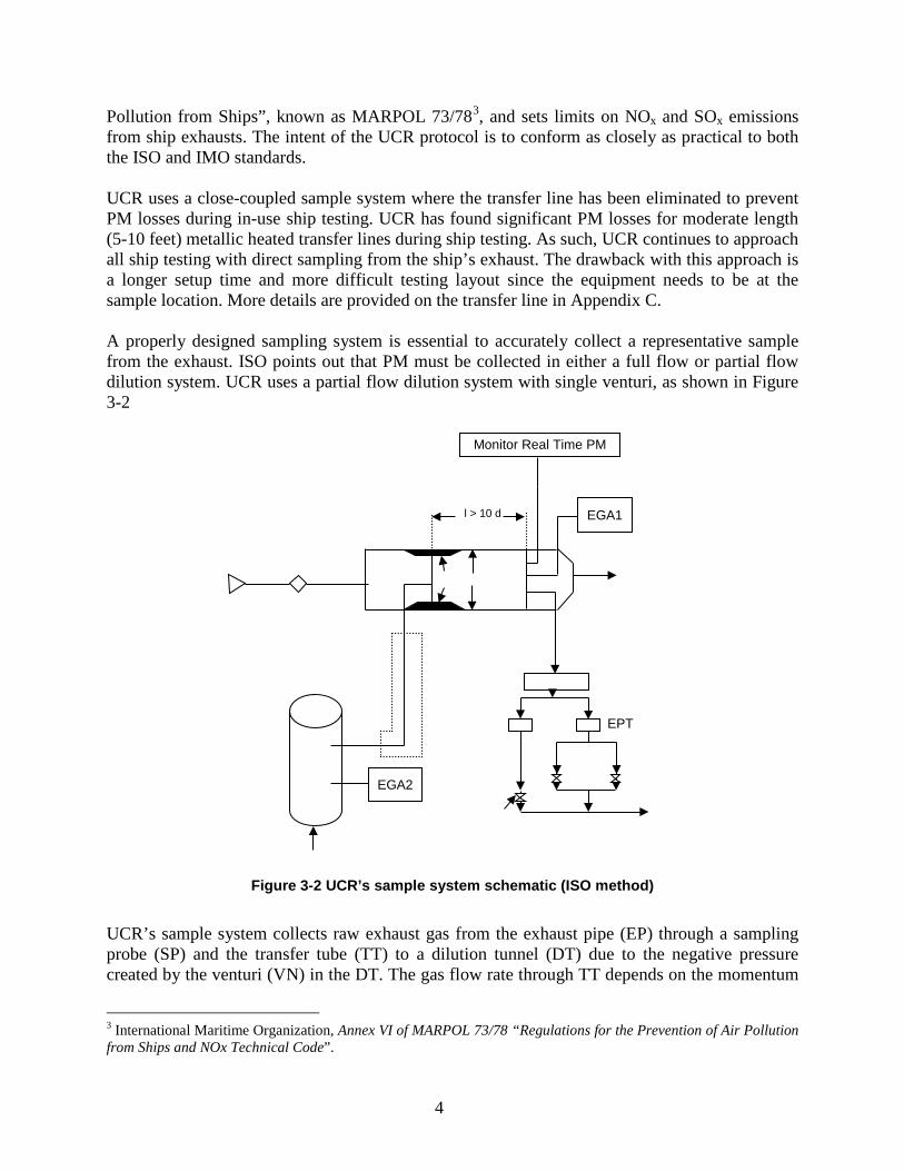
Pollution from Ships”, known as MARPOL 73/783, and sets limits on NOx and SOx emissions from ship exhausts. The intent of the UCR protocol is to conform as closely as practical to both the ISO and IMO standards. UCR uses a close-coupled sample system where the transfer line has been eliminated to prevent PM losses during in-use ship testing. UCR has found significant PM losses for moderate length (5-10 feet) metallic heated transfer lines during ship testing. As such, UCR continues to approach all ship testing with direct sampling from the ship’s exhaust. The drawback with this approach is a longer setup time and more difficult testing layout since the equipment needs to be at the sample location. More details are provided on the transfer line in Appendix C. A properly designed sampling system is essential to accurately collect a representative sample from the exhaust. ISO points out that PM must be collected in either a full flow or partial flow dilution system. UCR uses a partial flow dilution system with single venturi, as shown in Figure 3-2

Figure 3-2 UCR’s sample system schematic (ISO method)

UCR’s sample system collects raw exhaust gas from the exhaust pipe (EP) through a sampling probe (SP) and the transfer tube (TT) to a dilution tunnel (DT) due to the negative pressure created by the venturi (VN) in the DT. The gas flow rate through TT depends on the momentum

3 International Maritime Organization, Annex VI of MARPOL 73/78 “Regulations for the Prevention of Air Pollution from Ships and NOx Technical Code”.

EGA2

Monitor Real Time PM

l > 10 d EGA1

EPT

4

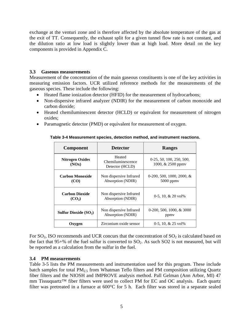
exchange at the venturi zone and is therefore affected by the absolute temperature of the gas at the exit of TT. Consequently, the exhaust split for a given tunnel flow rate is not constant, and the dilution ratio at low load is slightly lower than at high load. More detail on the key components is provided in Appendix C. 3.3 Gaseous measurements Measurement of the concentration of the main gaseous constituents is one of the key activities in measuring emission factors. UCR utilized reference methods for the measurements of the gaseous species. These include the following:

• Heated flame ionization detector (HFID) for the measurement of hydrocarbons; • Non-dispersive infrared analyzer (NDIR) for the measurement of carbon monoxide and

carbon dioxide; • Heated chemiluminescent detector (HCLD) or equivalent for measurement of nitrogen

oxides; • Paramagnetic detector (PMD) or equivalent for measurement of oxygen.

Table 3-4 Measurement species, detection method, and instrument reactions.

Component Detector Ranges

Nitrogen Oxides (NOx)

Heated Chemiluminescence

Detector (HCLD)

0-25, 50, 100, 250, 500, 1000, & 2500 ppmv

Carbon Monoxide (CO)

Non dispersive Infrared Absorption (NDIR)

0-200, 500, 1000, 2000, & 5000 ppmv

Carbon Dioxide (CO2)

Non dispersive Infrared Absorption (NDIR) 0-5, 10, & 20 vol%

Sulfur Dioxide (SO2) Non dispersive Infrared

Absorption (NDIR) 0-200, 500, 1000, & 3000

ppmv

Oxygen Zirconium oxide sensor 0-5, 10, & 25 vol%

For SO2, ISO recommends and UCR concurs that the concentration of SO2 is calculated based on the fact that 95+% of the fuel sulfur is converted to SO2. As such SO2 is not measured, but will be reported as a calculation from the sulfur in the fuel. 3.4 PM measurements Table 3-5 lists the PM measurements and instrumentation used for this program. These include batch samples for total PM2.5 from Whatman Teflo filters and PM composition utilizing Quartz fiber filters and the NIOSH and IMPROVE analysis method. Pall Gelman (Ann Arbor, MI) 47 mm Tissuquartz™ fiber filters were used to collect PM for EC and OC analysis. Each quartz filter was pretreated in a furnace at 600°C for 5 h. Each filter was stored in a separate sealed

5

petri dish at 10°C prior to and after sampling. A Sunset Labs (Forest Grove, OR) Thermal/Optical Carbon Aerosol Analyzer analyzed a 1.5 cm2 quartz filter punch following the temperature program outlined in the NIOSH 5040 method (NIOSH, 1996)4.A second 1.5 cm2 from the same filter was taken for analysis by the IMPROVE method. EC/OC was collected at 15 LPM onto precleaned (600 ºC, 8 hours) 47mm diameter QAT Tissuquartz quartz fiber filters (Pall-Gelman, Ann Arbor, MI, USA). OC analysis was performed using an Thermal/Optical Carbon Aerosol Analyzer (Sunset Laboratory, Forest Grove, OR, USA) in the thermal-optical transmittance (TOT) mode following the National Institute for Occupational Safety and Health (NIOSH) Method 5040 protocol (Birch and Cary, 1996,NIOSH method 5040. EC/OC was also analyzed using thermal-optical reflectance (TOR) following the DRI IMPROVE protocol on the Sunset Laboratories EC/OC analyzer modified to perform TOR correction and following the temperature program prescribed by the IMPROVE protocol (Chow, Watson, & Chen, 2015).

Table 3-5 PM Instruments and their measurement principles

3.5 PM measurements: Black Carbon There are several methods to measure black carbonaceous material and the reported terminology can be mixed. For example, the terms “black carbon, soot, elemental carbon, equivalent black carbon and refractory black carbon” refer to the light-absorbing component of particles, but the underlying definitions for these terms and associated measurement methods are different.5 Hence, BC measurements using different techniques are required to understand the nature and quantity of Black Carbon from emission sources. Published articles are available in the literature that describes the different BC measurement methods in detail.6

4 NIOSH (1996) NIOSH Manual of Analytical Methods. National Institute of Occupational Safety and Health, Cincinnati, OH. 5 Petzold, A., Ogren, J. A., Fiebig, M., Laj, P., Li, S.-M., Baltensperger, U., Holzer-Popp, T., Kinne, S., Pappalardo, G., Sugimoto, N., Wehrli, C., Wiedensohler, A., and Zhang, X.-Y. (2013) Recommendations for reporting "black carbon" measurements, Atmos. Chem. Phys., vol. 13, pp. 8365-8379, doi:10.5194/acp-13-8365-2013. 6 Moosmuller, H, Chakrabarty R, Arnott, W., (2009) Aerosol light absorption and its measurement: A review, Journal of Quantitative Spectroscopy and Radiative Transfer, vol. 110, pp 844-878.

6

Popular BC instrumentation methods use optical, thermal, or incandescence methods to estimate BC mass concentrations. BC emission inventories are mainly based on emission factors derived from thermal-optical methods that detect the carbon evolving from a heated filter sample, while data from atmospheric monitoring stations are mostly derived from optical absorption.7 For this project, real-time PM instruments were selected to characterize the black carbon emissions. These include the MSS 483 photoacoustic micro-soot sensor (BCPA-MSS) manufactured by AVL and the photoacoustic extinction meter (BCPA-PAX) by Droplet Measurement Technologies meter. Photoacoustic measurements use the intensity of a sound wave generated by the contraction and expansion of gas molecules when the BC particle is pulsed by a laser beam. The PA method has a large PM measurement range of the real time instruments and can measure up to 50,000 µg/m3, see Table 3-5. Other instruments require significant dilution of ship emissions to reach their desired BC concentration range (less than 100 µg/m3). The PA-soot method uses a conversion factor calibrated from gravimetric methods to derive the soot content. The PAX uses a photoacoustic meter in combination with light scattering. Thermo Scientific Multi-Angle Absorption Photometer (MAAP), and Magee Aethalometer (AE33) are other continuous filter based BC instruments that were not used for the testing on this voyage, but were used for a companion study on an auxiliary engine for the APL England. In addition to mass concentration the PAX reports the single scattering albedo which is important to understand the absorption of black carbon. Scattering albedo is proportional to the absorption coefficient divided by the sum of the absorption coefficient and the scattering coefficient. These results will be presented in this report separately form the mass concentration.

7 Petzold, A., Ogren, J. A., Fiebig, M., Laj, P., Li, S.-M., Baltensperger, U., Holzer-Popp, T., Kinne, S., Pappalardo, G., Sugimoto, N., Wehrli, C., Wiedensohler, A., and Zhang, X.-Y. (2013) Recommendations for reporting "black carbon" measurements, Atmos. Chem. Phys., vol. 13, pp. 8365-8379, doi:10.5194/acp-13-8365-2013.

7

4 Quality Control This section describes UCR standard practices for calibrations, verifications, and control checks performed before, during and after testing. This section also describes checks performed to validate the data provided in the report. Additional instrument accuracy, precision, and standard verifications is provided in Appendix C. 4.1 Pre-test calibrations Prior to departing from UCR all systems were cleaned and verified for the testing campaign. The MSS system included cleaning the internal pollution window and performing a span calibration using an internal pollution window. All systems were found to be within specifications and the systems were prepared for testing. 4.2 On-site calibrations Pre- and post-test calibrations were performed on the gaseous analyzer using NIST traceable calibration bottles. Post-test dilution ratio was verified by removing the probe from the dilution tunnel and sampling from the raw exhaust. This method has been used in addition to operating two gas analyzers and has been shown to be reliable. Hourly zero checks were performed with each of the real time PM instruments. Leak checks were performed for the total PM2.5 system prior to each sample point. 4.3 Post-test and data validation Post-test evaluation includes verifying consistent dilution ratios between points and verifying brake specific fuel consumption (BSFC) with reported manufacturer numbers. Typically, this involves corresponding with the engine manufacturer to discuss the results for emissions of interest. The brake specific fuel consumption results were with-in reason and thus suggest the load and mass of emissions measured are reasonable and representative. Thus, this suggests the data collected for the APL England main engine out emissions are accurate and representative of a properly functioning system.

8

5 Results

This section covers the emission results for the tests on the main engines on the APL England container vessel on the MGO and HFO fuels. The results are organized into four sections, 1) Gaseous and PM emissions, 2) PM2.5 and OC emissions, and 3) Black Carbon measurement techniques. 5.1 Real-time emissions Figure 5-1, Figure 5-2, and Figure 5-3 show the real time PM-soot, NOx and CO2 emissions as a function of time for the main engine tested. The results of full voyage condition are presented by Figure 5-1. For the full voyage, the dilute NOx concentration varied from 50 to 200 ppm and the dilute CO2 concentration varied from 0.06% to 1.0% during dilute sampling. The PA-soot concentration varied from 0 mg/m3 to 0.8 mg/m3. The PAX PA-soot concentration also varied from 0 mg/m3 to 0.8 mg/m3, but it was slightly higher than MSS PA-soot concentration. The green stars represent when filter batch samples were collected for the Teflon and Quartz filter media. Typically three samples are collected, but due to limited time and vessel crew demands, some tests only utilized two filter samples. The large spikes in the gaseous emissions are a result of the dilution ratio quantification. The dilution ratio was checked after each batch PM filter sample by moving the dilute sample probe to the stack for raw sampling. The raw CO2 concentrations reached 6% which resulted in spikes from less than 1% to ~6% in a short amount of time.

Figure 5-1 Real time emissions measurement during the full voyage

9

Figure 5-2 and Figure 5-3 show the time representing the departure from Oakland and arrival at San Pedro, respectively. BC emissions based on PA-soot and MSS soot concentrations for these specific parts of the voyage fluctuated a lot and were relatively higher than other time periods for the voyage. When the ship departed Oakland, BC showed a maximum concentration of 0.8 mg/m3, which was higher than for the remainder of the voyage. For gaseous emissions, NOx and CO2 concentrations, showed a series of peaks when the ship departed Oakland and arrived at San Pedro.

Figure 5-2 Real time emissions measurement when departing Oakland

10

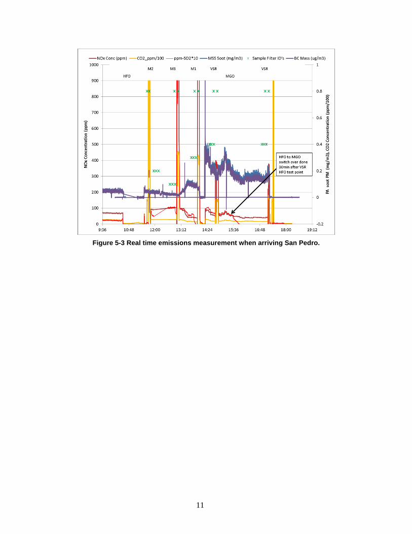
Figure 5-3 Real time emissions measurement when arriving San Pedro.

11

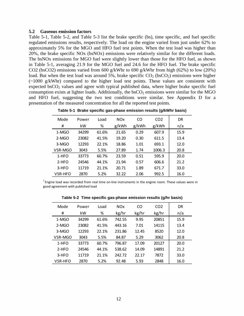
5.2 Gaseous emission factors Table 5-1, Table 5-2, and Table 5-3 list the brake specific (bs), time specific, and fuel specific regulated emissions results, respectively. The load on the engine varied from just under 62% to approximately 5% for the MGO and HFO fuel test points. When the test load was higher than 20%, the brake specific NOx (bsNOx) emissions were relatively similar for the different loads. The bsNOx emissions for MGO fuel were slightly lower than those for the HFO fuel, as shown in Table 5-1, averaging 21.9 for the MGO fuel and 24.6 for the HFO fuel. The brake specific CO2 (bsCO2) emissions varied from 600 g/kWhr to 690 g/kWhr from high (62%) to low (20%) load. But when the test load was around 5%, brake specific CO2 (bsCO2) emissions were higher (~1000 g/kWhr) compared to the higher load test points. These values are consistent with expected bsCO2 values and agree with typical published data, where higher brake specific fuel consumption exists at lighter loads. Additionally, the bsCO2 emissions were similar for the MGO and HFO fuel, suggesting the two test conditions were similar. See Appendix D for a presentation of the measured concentration for all the reported test points.

Table 5-1 Brake specific gas-phase emission results (g/kWhr basis)

1 Engine load was recorded from real time on-line instruments in the engine room. These values were in good agreement with published load

Table 5-2 Time specific gas-phase emission results (g/hr basis)

Mode Power Load NOx CO CO2 DR# kW % g/kWh g/kWh g/kWh n/a

1-MGO 34299 61.6% 21.65 0.29 607.9 15.92-MGO 23082 41.5% 19.20 0.30 611.5 13.43-MGO 12293 22.1% 18.86 1.01 693.1 12.0

VSR-MGO 3043 5.5% 27.89 1.74 1006.3 20.81-HFO 33773 60.7% 23.59 0.51 595.9 20.02-HFO 24546 44.1% 21.94 0.57 606.6 21.23-HFO 11719 21.1% 20.71 1.89 671.7 33.0

VSR-HFO 2870 5.2% 32.22 2.06 992.5 16.0

Mode Power Load NOx CO CO2 DR# kW % kg/hr kg/hr kg/hr n/a

1-MGO 34299 61.6% 742.55 9.95 20851 15.92-MGO 23082 41.5% 443.16 7.01 14115 13.43-MGO 12293 22.1% 231.86 12.45 8520 12.0

VSR-MGO 3043 5.5% 84.87 5.29 3062 20.81-HFO 33773 60.7% 796.87 17.09 20127 20.02-HFO 24546 44.1% 538.62 14.09 14891 21.23-HFO 11719 21.1% 242.72 22.17 7872 33.0

VSR-HFO 2870 5.2% 92.48 5.93 2848 16.0

12

Table 5-3 Fuel specific gas-phase emission results (g/kg fuel basis)

5.2.1 CO2 Figure 5-4 plots the bsCO2 emissions versus load for the MGO and the HFO. The HFO appears to use slightly less fuel as would be expected due to the higher energy content of HFO compared to MGO. The overlap of the CO2 standard deviations for MGO and HFO at each load, indicate there is no statistically significant difference in the bsCO2 emissions for MGO and HFO at any of the tested engine load points.

Figure 5-4 Brake Specific CO2 Emissions versus Engine Load

5.2.2 NOx Figure 5-5 plots the bsNOx emissions versus load for the MGO and the HFO. The NOx emissions are higher from the HFO than from the MGO at all engine load points, but only the differences at the 5% and 40% engine load points are statistically different.

Mode Power Load NOx CO CO2 DR# kW % g/kg fuel g/kg fuel g/kg furl n/a

1-MGO 34299 61.6% 116.04 1.55 3258.4 15.92-MGO 23082 41.5% 100.14 1.58 3189.5 13.43-MGO 12293 22.1% 89.77 4.82 3298.8 12.0

VSR-MGO 3043 5.5% 91.41 5.70 3297.7 20.81-HFO 33773 60.7% 126.37 2.71 3191.8 20.02-HFO 24546 44.1% 115.01 3.01 3179.5 21.23-HFO 11719 21.1% 98.28 8.98 3187.5 33.0

VSR-HFO 2870 5.2% 105.48 6.76 3249.0 16.0

13

Figure 5-5 Brake Specific NOx Emissions versus Engine Load

5.2.3 CO Figure 5-6 plots the bsCO emissions versus load for the MGO and the HFO. As was the case for the bsNOx the bsCO emissions are higher from the HFO than from the MGO. The differences are statistically different at the 5% engine load point and may be marginally statistically different at the 60% engine load point.

Figure 5-6 Brake Specific CO Emissions versus Engine Load

5.3 PM emission factors Table 5-4 shows the brake specific emissions of PM2.5, BCPA-MSS, BCPA-PAX, and EC/OC by NIOSH and IMPROVE for both the MGO and HFO fuels. The engine out bsPM2.5 ranged from 207 mg/kWhr to 501 mg/kWhr over the range of loads and test fuels tested. The higher bsPM2.5 emissions at lighter loads for the HFO agrees with typical diesel engine emission rates. However,

14

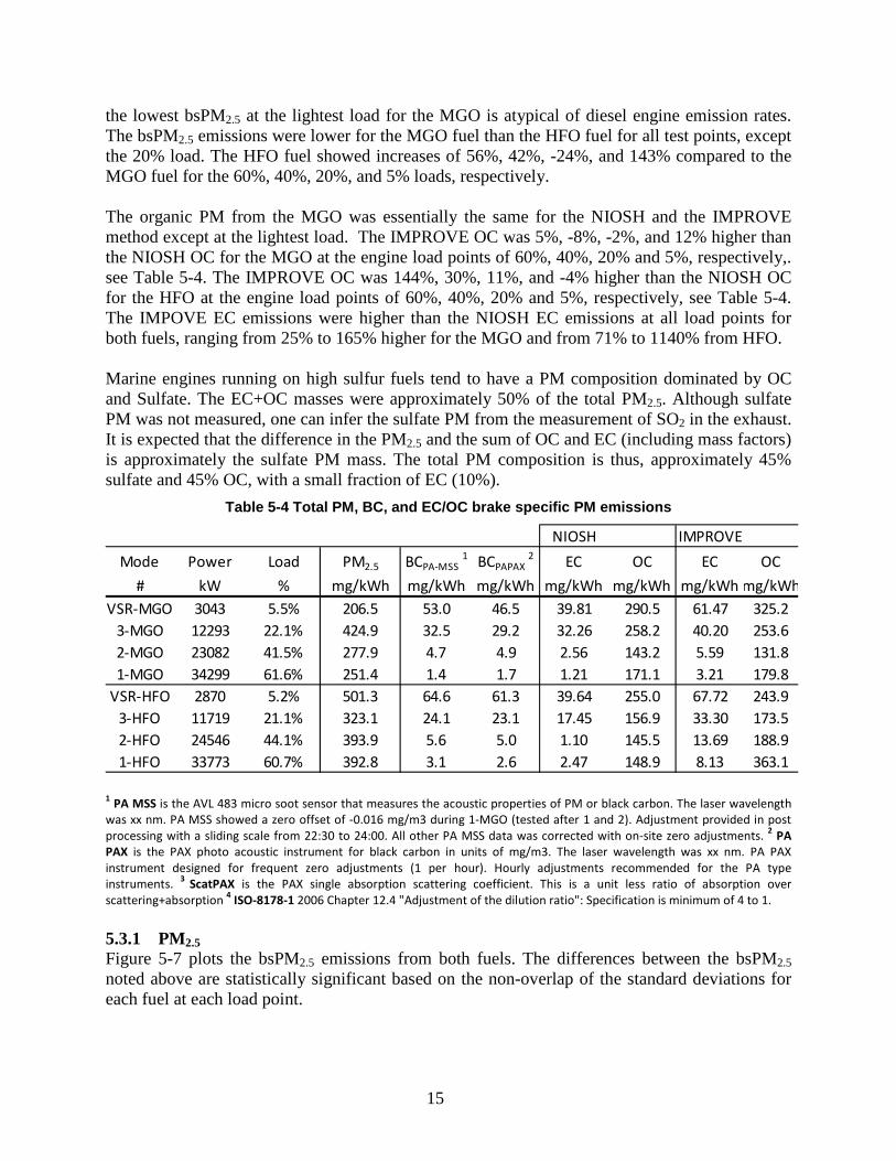
the lowest bsPM2.5 at the lightest load for the MGO is atypical of diesel engine emission rates. The bsPM2.5 emissions were lower for the MGO fuel than the HFO fuel for all test points, except the 20% load. The HFO fuel showed increases of 56%, 42%, -24%, and 143% compared to the MGO fuel for the 60%, 40%, 20%, and 5% loads, respectively. The organic PM from the MGO was essentially the same for the NIOSH and the IMPROVE method except at the lightest load. The IMPROVE OC was 5%, -8%, -2%, and 12% higher than the NIOSH OC for the MGO at the engine load points of 60%, 40%, 20% and 5%, respectively,. see Table 5-4. The IMPROVE OC was 144%, 30%, 11%, and -4% higher than the NIOSH OC for the HFO at the engine load points of 60%, 40%, 20% and 5%, respectively, see Table 5-4. The IMPOVE EC emissions were higher than the NIOSH EC emissions at all load points for both fuels, ranging from 25% to 165% higher for the MGO and from 71% to 1140% from HFO. Marine engines running on high sulfur fuels tend to have a PM composition dominated by OC and Sulfate. The EC+OC masses were approximately 50% of the total PM2.5. Although sulfate PM was not measured, one can infer the sulfate PM from the measurement of SO2 in the exhaust. It is expected that the difference in the PM2.5 and the sum of OC and EC (including mass factors) is approximately the sulfate PM mass. The total PM composition is thus, approximately 45% sulfate and 45% OC, with a small fraction of EC (10%).

Table 5-4 Total PM, BC, and EC/OC brake specific PM emissions

1 PA MSS is the AVL 483 micro soot sensor that measures the acoustic properties of PM or black carbon. The laser wavelength was xx nm. PA MSS showed a zero offset of -0.016 mg/m3 during 1-MGO (tested after 1 and 2). Adjustment provided in post processing with a sliding scale from 22:30 to 24:00. All other PA MSS data was corrected with on-site zero adjustments. 2 PA PAX is the PAX photo acoustic instrument for black carbon in units of mg/m3. The laser wavelength was xx nm. PA PAX instrument designed for frequent zero adjustments (1 per hour). Hourly adjustments recommended for the PA type instruments. 3 ScatPAX is the PAX single absorption scattering coefficient. This is a unit less ratio of absorption over scattering+absorption 4 ISO-8178-1 2006 Chapter 12.4 "Adjustment of the dilution ratio": Specification is minimum of 4 to 1. 5.3.1 PM2.5 Figure 5-7 plots the bsPM2.5 emissions from both fuels. The differences between the bsPM2.5 noted above are statistically significant based on the non-overlap of the standard deviations for each fuel at each load point.

NIOSH IMPROVEMode Power Load PM2.5 BCPA-MSS 1 BCPAPAX 2 EC OC EC OC

# kW % mg/kWh mg/kWh mg/kWh mg/kWh mg/kWh mg/kWh mg/kWhVSR-MGO 3043 5.5% 206.5 53.0 46.5 39.81 290.5 61.47 325.2

3-MGO 12293 22.1% 424.9 32.5 29.2 32.26 258.2 40.20 253.62-MGO 23082 41.5% 277.9 4.7 4.9 2.56 143.2 5.59 131.81-MGO 34299 61.6% 251.4 1.4 1.7 1.21 171.1 3.21 179.8

VSR-HFO 2870 5.2% 501.3 64.6 61.3 39.64 255.0 67.72 243.93-HFO 11719 21.1% 323.1 24.1 23.1 17.45 156.9 33.30 173.52-HFO 24546 44.1% 393.9 5.6 5.0 1.10 145.5 13.69 188.91-HFO 33773 60.7% 392.8 3.1 2.6 2.47 148.9 8.13 363.1

15

Figure 5-7 PM2.5 as a Function of Engine Load for MGO and HFO

5.3.2 BC Figure 5-8 plots BC emissions for both fuels and two test methods for all engine load points. Both methods give essentially the same bsBC at all engine load points for the same fuel. At the 5% engine load point both methods show higher bsBC emissions for the HFO fuel while at all other load points the bsBC are statistically the same for both fuels.

Figure 5-8 BC by two methods as a Function of Engine Load for MGO and HFO

5.3.3 EC Figure 5-9 plots the bsEC emissions for both fuels by the IMPROVE and the NIOSH methods. The results are mixed. At the 5% load the NIOSH method gives much lower results for both fuels and only the IMPROVE method gives higher emissions for the HFO versus the MGO. At the 20% load the NIOSH method gives lower results for both fuels but only much lower for the

0

100

200

300

400

500

600

5.0% 20.0% 40.0% 60.0%

PM2.

5 Em

issio

ns (m

g/kW

h)

Engine Load (%)

MGO

HFO

16

HFO. Both the IMPROVE and the NIOSH show higher emissions for the MGO versus the HFO at the 20% load. At the 40% load the NIOSH shows lower emissions than the IMPROVE for both fuels but for MGO the differences are not statistically different. The IMPROVE has statistically higher emissions for the HFO versus the MGO at the 40% load while the NIOSH has higher emissions from the MGO than from the HFO but the difference is not statistically significant. At the 60% load the NIOSH method results are lower than the IMPROVE results for both fuels and both methods have higher emissions for the HFO versus the MGO. Since the samples for the EC/OC analysis were taken from the same filter these results indicate that the calculated µg of EC on the filter is dependent upon the method used to measure it.

Figure 5-9 EC by two methods as a Function of Engine Load for MGO and HFO

Figure 5-10 plots the bsBCPA-MSS versus the IMPROVE bsEC for both fuels and there is a very high correlation between the methods for both fuels. However, while there is nearly a 1 to 1 correlation for the HFO fuel the bsBCPA-MSS results are ~13% lower than the bsEC. As is seen in Table 5-5, while there is variation in the slopes and intercepts for all other possible correlations, they all have very high correlation coefficients.

17

Figure 5-10 Black Carbon by PA-MSS versus EC by IMPROVE

Table 5-5 BC Photoacoustic Correlation Equations with EC by Improve and NIOSH Methods

BC Method EC Method Fuel y = R2

PA-MSS IMPROVE MGO 0.8661x – 0.993 0.9982 HFO 1.0512x – 7.9558 0.9928

PA-MSS NIOSH MGO 1.2008x + 0.1575 0.9619 HFO 1.576x + 0.4264 0.9874

PA-PAX IMPROVE MGO 0.7504x –0.1462 0.9985 HFO 1.0033x – 7.8064 0.9937

PA-PAX NIOSH MGO 1.0419x + 0.8228 0.9649 HFO 1.50456x + 0.189 0.9887

5.3.4 OC Figure 5-11 plots the OC emissions versus engine load for both fuels by the IMPROVE and NIOSH methods. Because OC depends on the dilution ratio, which wasn’t constant for all tests, (see chapter 5), quantitative comparisons of these emissions are not valid.

18

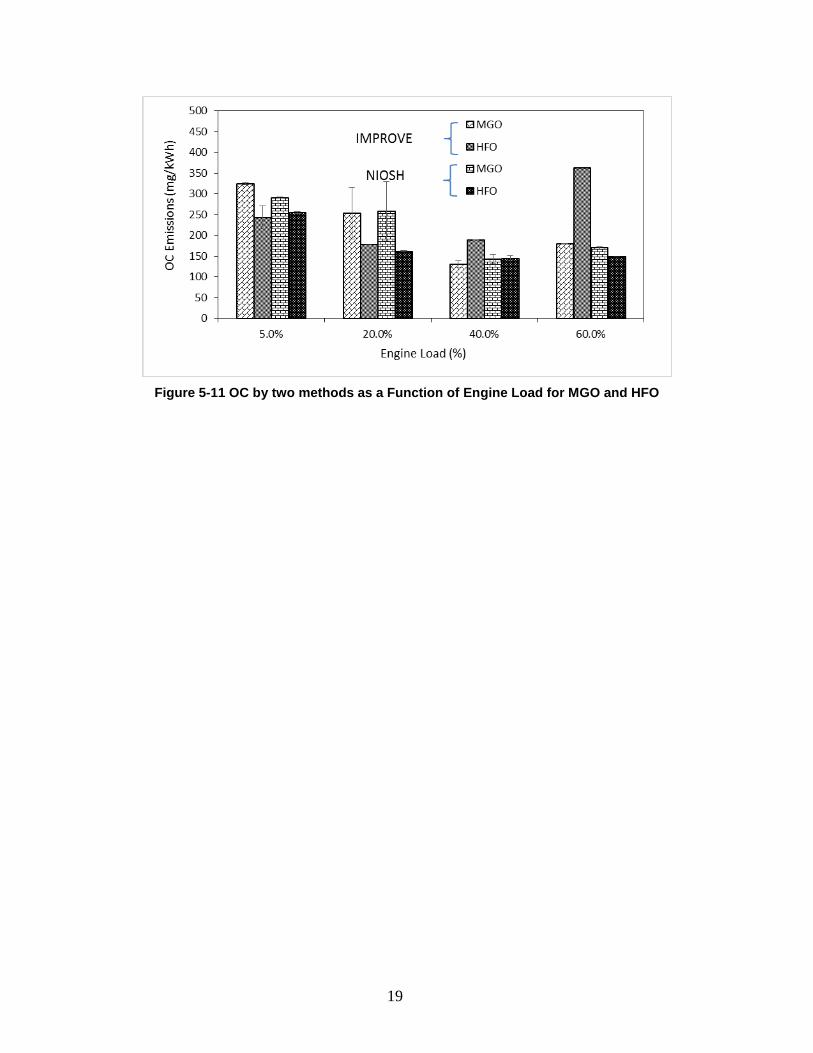
Figure 5-11 OC by two methods as a Function of Engine Load for MGO and HFO

19

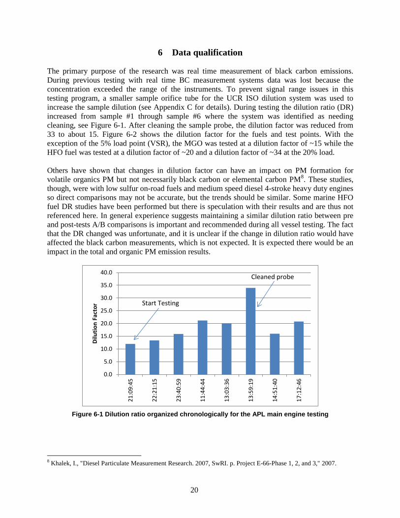
6 Data qualification The primary purpose of the research was real time measurement of black carbon emissions. During previous testing with real time BC measurement systems data was lost because the concentration exceeded the range of the instruments. To prevent signal range issues in this testing program, a smaller sample orifice tube for the UCR ISO dilution system was used to increase the sample dilution (see Appendix C for details). During testing the dilution ratio (DR) increased from sample #1 through sample #6 where the system was identified as needing cleaning, see Figure 6-1. After cleaning the sample probe, the dilution factor was reduced from 33 to about 15. Figure 6-2 shows the dilution factor for the fuels and test points. With the exception of the 5% load point (VSR), the MGO was tested at a dilution factor of ~15 while the HFO fuel was tested at a dilution factor of ~20 and a dilution factor of ~34 at the 20% load. Others have shown that changes in dilution factor can have an impact on PM formation for volatile organics PM but not necessarily black carbon or elemental carbon PM8. These studies, though, were with low sulfur on-road fuels and medium speed diesel 4-stroke heavy duty engines so direct comparisons may not be accurate, but the trends should be similar. Some marine HFO fuel DR studies have been performed but there is speculation with their results and are thus not referenced here. In general experience suggests maintaining a similar dilution ratio between pre and post-tests A/B comparisons is important and recommended during all vessel testing. The fact that the DR changed was unfortunate, and it is unclear if the change in dilution ratio would have affected the black carbon measurements, which is not expected. It is expected there would be an impact in the total and organic PM emission results.

Figure 6-1 Dilution ratio organized chronologically for the APL main engine testing

8 Khalek, I., "Diesel Particulate Measurement Research. 2007, SwRI. p. Project E-66-Phase 1, 2, and 3," 2007.

0.0

5.0

10.0

15.0

20.0

25.0

30.0

35.0

40.0

21:0

9:45

22:2

1:15

23:4

0:59

11:4

4:44

13:0

3:36

13:5

9:19

14:5

1:40

17:1

2:46

Dilu

tion

Fact

or Start Testing

Cleaned probe

20

Figure 6-2 Dilution ratio organized by test mode for the APL main engine testing

21

7 Summary and Conclusions

Emissions from a marine main engine operating on marine gas oil (MGO) and a heavy fuel oil (HFO) were measured on an ocean voyage from Oakland, CA to San Pedro, CA. Emissions measurements included SOx, THCs, NOx, CO2, and PM, including PM2.5 mass (2.5 µm fine particles only), elemental, organic and BC. BC was measured by two photoacoustic instruments and by extraction from a quartz filter followed by FID determination by the NIOSH and IMPROVE methods. The overall results and conclusions from this work can be summarized in the following highlights:

• Brake specific NOx (bsNOx) emissions were relatively similar for the different loads for test loads higher than 20%. The bsNOx emissions for MGO fuel were slightly lower than those for the HFO fuel, averaging 21.9 for the MGO fuel and 24.6 for the HFO fuel.

• Brake specific CO2 (bsCO2) emissions varied from ~600 g/kWhr to ~690 g/kWhr from high (62%) to low (20%) load. But when the test load was around 5%, brake specific CO2 (bsCO2) emissions were ~1000 g/KWh. These values are consistent with expected bsCO2 values and agree with typical published data, where higher brake specific fuel consumption exists at lighter loads. Additionally, the bsCO2 emissions were similar for the MGO and HFO fuel, suggesting the two test conditions were similar.

• BC measurements and the existing ISO 8178 sampling procedures work well for in-situ Photoacoustic type meters.

• For the same fuel at the same engine load, the two photoacoustic meters give essentially the same results.

• At the 5% engine load point both photoacoustic meters showed higher BC emissions for the HFO fuel while at all other load points the BC emissions are statistically the same for both fuels.

• EC as determined by the NIOSH and IMPROVE method correlated well with the BC measurements for both fuels. The R-squared correlation coefficients are between 0.9619 and 0.9937 for correlations of bsBC with bsEC. The slopes of the equations vary between 0.7504 and 1.576 depending upon the BC and EC method and the fuel.

• The differences in the bsEC between the NIOSH and IMPROVE method is related to the method and not the sample since the samples were taken from the same quartz filter.

22

Appendix A. Ship and Fuel Specifications This Appendix contains records utilized during the testing of the ocean going vessel. These records were either obtained from the engine control room manuals (engine related details) or from the captain’s fuel records during bunkering. Selected items were greyed out for each vessel manufacturer. Only the pertinent information relating to the testing was provided.

Figure A-1 HFO analysis reference

Figure A-2 MGO analysis reference

A-1

Figure A-3 Ship particulars and specifications

A-2

Figure A-4 Engine information

A-3

Figure A-4 Engine specifications relevant to emissions testing

A-4

Appendix B. Test logs This Appendix summarizes the details of the test logs utilized for the analysis. Table B-1 shows the engine details measured from the vessels engine control room. Table B-2 shows the sample log for the Teflon and Quartz filters sampled as part of the PM measurement systems. The footnotes provide contract for special observations with each log record.

Table B-1 Log samples of engine load, fuel rate, BSFC, and exhaust flow parameters

1 According to the engine manual (report # ENG-00160) Samsung - MAN B&W the engine RPM ranges from 25 rpm (idle) to 94 RPM max

Fuel Rate Torque BSFC Fixed 1 Meas SpdTime kg/hr kN*m g/kWhr Intake P_bar Intake T_C RPM knots Fuel Operation19:52 3047 2390 198 0.5 34 62.1 MGO Leave Port19:54 3223 2402 197.8 0.5 34 63.7 MGO Leave Port19:58 3374 2409 196.9 0.7 34 65 MGO Leave Port20:09 3573 2427 195.9 0.82 34 64 MGO Leave Port20:18 2260 2374 200 0.4 34 57 MGO Leave Port20:21 2702 2378 220 0.41 34 57.7 MGO Leave Port20:22 1155 2294 313 0.2 34 42 MGO Leave Port20:26 1100 2200 300 0.20 34 45 MGO Leave Port20:27 100 2200 450 0.10 34 28 MGO Leave Port20:34 800 200 350 0.01 34 34 MGO Leave Port20:36 1100 2200 300 0.20 34 45 MGO Leave Port20:36 2260 2374 200 0.4 34 58 MGO Leave Port20:37 2260 2374 200 0.4 34 58 MGO set RPM 20:40 0.4 35 60 16.3 MGO mode 320:44 2712 2375 220 0.4 35 59.6 MGO mode 320:46 2580 2370 210 0.4 35 59.5 MGO mode 320:48 2618 2364 210 0.4 35 59.9 MGO mode 320:50 2550 2371 209 0.4 35 59.4 MGO mode 320:53 2600 2366 210 0.4 35 59.4 MGO mode 320:55 2630 2379 210 0.4 35 59 MGO mode 320:56 2611 2370 220 0.4 35 58.9 MGO mode 320:56 210 0.4 35 60 MGO mode 321:23 2611 2370 210 0.4 35 60 MGO set new RPM21:52 3944 2426 171 1 37 72 19.8 MGO mode 222:09 3967 2423 171 1 37 72 MGO mode 222:41 3930 171 1 37 72 MGO mode 222:41 3930 2423 171 1 37 72 MGO set new RPM23:13 5120 2471 150 1.6 41 80 22.4 MGO mode 123:34 5100 2475 149.5 1.6 41 79.1 MGO mode 123:50 5180 2470 149.5 1.6 41 79.9 MGO mode 123:51 5180 2470 149.5 1.6 41 79.9 MGO set fuel and RPM0:20 0.8 36 70 HFO in-use8:32 3550 181 0.8 37 69 HFO

11:32 3325 190.5 0.71 37 67 HFO set new RPM11:46 3941 2418 180.4 0.92 38 70.4 HFO setting new RPM11:50 4313 2441 172 1.05 38 71.9 19.1 HFO mode 212:02 4054 2436 172.1 1.02 38 72 19.6 HFO mode 212:15 4306 2443 172.2 1.08 39 71.8 19.9 HFO set new RPM12:40 5298 2473 155.9 1.5 42 79.4 21.7 HFO mode 112:47 5256 2474 156.6 1.5 43 79.2 21.7 HFO mode 112:56 2483 156.1 1.55 43 79.6 HFO mode 113:04 5365 2479 150.4 1.57 43 79.6 21.6 HFO set new RPM13:36 2510 2360 212.9 0.4 41 59.5 16.2 HFO mode 313:42 2454 2362 212.8 0.5 41 59.3 HFO mode 313:47 2478 2370 212.7 0.5 41 59.5 16.8 HFO mode 313:59 2539 2364 213.3 0.5 41 59.3 16.8 HFO set VSR speed14:21 904 2287 315 0.15 40 40 11.6 HFO set VSR speed17:08 946 2294 310.9 0.15 37 40.7 11.6 MGO mode VSR

Engine

B-1

Table B2 Filter log and summary weights

1 Note: Red highlighted samples were outliers and were removed from the analysis. Blue are filters that were damaged and not weighed.

Table Filter media and flows for each test point sampled

Test Day Mode Fuel Start End Teflon ID Quartz IDPM total mg/filter

PM EC mg/filter

PM OC mg/filter

PM EC mg/filter

PM OC mg/filter

1 Teflo V m3

1 Quartz V m3

PM total mg/m3

PM EC mg/m3

PM OC mg/m3

PM EC mg/m3

PM OC mg/m3

1 15 3 MGO 20:44:30 20:47:30 WT130272 QU201310_01 0.300 0.024 0.182 0.028 0.167 0.049 0.045 6.13 0.53 4.07 0.63 3.752 15 3 MGO 20:54:00 20:57:00 WT130271 QU201310_02 0.222 0.014 0.113 0.018 0.114 0.049 0.045 4.55 0.32 2.53 0.40 2.553 15 3 MGO 21:01:00 21:04:00 WT130274 QU201310_03 0.221 0.015 0.123 0.019 0.129 0.049 0.045 4.53 0.33 2.75 0.43 2.89

15 PreDR15 ChkDR


15 PreDR15 DR


16 PreDR16 DR

10 16 2 HFO 11:57:00 12:00:00 WT130283 QU201310_11 0.162 0.000 0.064 0.006 0.075 0.049 0.045 3.31 0.01 1.43 0.14 1.6711 16 2 HFO 12:03:30 12:06:30 WT130284 QU201310_12 0.170 0.001 0.052 0.004 0.067 0.049 0.045 3.47 0.02 1.17 0.09 1.4912 16 2 HFO 12:10:00 12:13:00 WT130286 QU201310_13 0.155 0.050 0.005 0.075 0.049 0.045 3.16 0.00 1.12 0.12 1.67

16 PreDR16 DR

13 16 1 HFO 12:41:30 12:44:30 WT130287 QU201310_14 0.188 0.001 0.065 0.003 0.074 0.049 0.045 3.85 0.02 1.45 0.07 1.6514 16 1 HFO 12:48:30 12:51:30 WT130288 QU201310_15 0.171 0.001 0.060 0.003 0.073 0.049 0.045 3.50 0.03 1.34 0.07 1.6415 16 1 HFO 12:55:30 12:58:30 WT130289 QU201310_16 0.170 0.001 0.061 0.004 0.306 0.049 0.045 3.48 0.02 1.37 0.09 6.85

16 PreDR16 DR

16 16 3 HFO 13:40:00 13:43:00 WT130292 QU201310_17 0.074 0.005 0.036 0.007 0.038 0.049 0.045 1.52 0.12 0.81 0.16 0.8517 16 3 HFO 13:46:00 13:49:00 WT130290 QU201310_18 0.058 0.002 0.026 0.007 0.033 0.049 0.045 1.19 0.05 0.58 0.16 0.7418 16 3 HFO 13:53:00 13:56:00 WT130291 QU201310_19 0.068 0.002 0.028 0.005 0.029 0.049 0.045 1.39 0.05 0.63 0.11 0.64

16 PreDR16 DR

19 16 VSR HFO 14:30:00 14:33:00 WT130293 QU201310_20 0.123 0.049 0.045 2.5120 16 VSR HFO? 14:34:30 14:37:30 WT130294 QU201310_21 0.085 0.049 0.045 1.7321 16 VSR HFO? 14:42:00 14:45:00 WT130295 QU201310_22 0.069 0.007 0.043 0.012 0.041 0.049 0.045 1.40 0.15 0.97 0.26 0.93

16 PreDR16 DR

22 16 VSR MGO 16:54:30 16:57:30 WT130296 QU201310_25 0.050 0.005 0.037 0.009 0.041 0.049 0.045 1.02 0.10 0.82 0.19 0.9223 16 VSR MGO 17:00:00 17:03:00 WT130297 QU201310_26 0.005 0.006 0.042 0.007 0.043 0.049 0.045 0.10 0.14 0.95 0.16 0.9524 16 VSR MGO 17:06:30 17:09:30 WT130298 QU201310_27 0.036 -0.296 105.730 0.009 0.049 0.049 0.045 0.74 -6.63 2365.32 0.21 1.10

16 PreDR16 DR

NIOSH IMPROVE

Filters not in labFilters not in lab

Anatlical NIOSH IMPROVE

B-2

Appendix C. Sampling system description ISO 8178-1 9 and ISO 8178-2 10 specify the measurement and evaluation methods for gaseous and particulate exhaust emissions when combined with combinations of engine load and speed provided in IS0 8178- Part 4: Test cycles for different engine applications. The emission results represent the mass rate of emissions per unit of work accomplished. Specific emission factors are based on brake power measured at the crankshaft, the engine being equipped only with the standard auxiliaries necessary for its operation. Per ISO, auxiliary losses are <5 % of the maximum observed power. IMO ship pollution rules and measurement methods are contained in the “International Convention on the Prevention of Pollution from Ships”, known as MARPOL 73/7811, and sets limits on NOx and SOx emissions from ship exhausts. The intent of this protocol was to conform as closely as practical to both the ISO and IMO standards. Gaseous and Particulate Emissions A properly designed sampling system is essential to accurate collection of a representative sample from the exhaust and subsequent analysis. ISO points out that particulate must be collected in either a full flow or partial flow dilution system and UCR chose the partial flow dilution system with single venturi as shown in Figure C-1.

9 International Standards Organization, IS0 8178-1, Reciprocating internal combustion engines - Exhaust emission measurement -Part 1: Test-bed measurement of gaseous particulate exhaust emissions, First edition 1996-08-l5 10 International Standards Organization, IS0 8178-2, Reciprocating internal combustion engines - Exhaust emission measurement -Part 2: Measurement of gaseous and particulate exhaust emissions at site, First edition 1996-08-l5 11 International Maritime Organization, Annex VI of MARPOL 73/78 “Regulations for the Prevention of Air Pollution from Ships and NOx Technical Code”.

C-1

Figure C-1 Partial Flow Dilution System with Single Venturi

A partial flow dilution system was selected based on cost and the impossibility of a full flow dilution for “medium and large” engine testing on the test bed and at site. The flow in the dilution system eliminates water condensation in the dilution and sampling systems and maintains the temperature of the diluted exhaust gas at <52°C before the filters. ISO cautions the advantages of partial flow dilution systems can be lost to potential problems such as: losing particulates in the transfer tube, failing to take a representative sample from the engine exhaust and inaccurately determining the dilution ratio. An overview of UCR’s partial dilution system in Figure C-1 shows that raw exhaust gas is transferred from the exhaust pipe (EP) through a sampling probe (SP) and the transfer tube (TT) to a dilution tunnel (DT) due to the negative pressure created by the venturi (VN) in DT. The gas flow rate through TT depends on the momentum exchange at the venturi zone and is therefore affected by the absolute temperature of the gas at the exit of TT. Consequently, the exhaust split for a given tunnel flow rate is not constant, and the dilution ratio at low load is slightly lower than at high load. More detail on the key components is provided in Table C-1.

EGA2

d

Real Time PM

Air Filter

DT

l > 10 d

Exhaust

SP

EGA1

VN

TT

Secondary dilution

Vent

Quartz PTF

To Vacuum Pump

Cyclone

CFO

EP

C-2

Figure C-2 Dilution system and measurement layout on the auxiliary engine exhaust stack

Dilution Air System A partial flow dilution system requires dilution air and UCR uses compressed air in the field as it is readily available. ISO recommends the dilution air be at 25 ±5°C, filtered and charcoal scrubbed to eliminate background hydrocarbons. The dilution air may be dehumidified. To ensure the compressed air is of a high quality UCR processes any supplied air through a field processing unit that reduces the pressure to about 30psig as that level allows a dilution ratio of about 5/1 in the geometry of our system. The next stages, in sequence, include: a liquid knock-out vessel, desiccant to remove moisture with silica gel containing an indicator, hydrocarbon removal with activated charcoal and a HEPA filter for the fine aerosols that might be present in the supply air. The silica gel and activated carbon are changed for each field campaign. Figure C-3 shows the field processing unit in its transport case. In the field the case is used as a framework for supporting the unit

Direct sampling

C-3

Figure C-3 Field Processing Unit for Purifying Dilution Air in Carrying Case

C-4

Table C-1 Components of a Sampling System: ISO/IMO Criteria & UCR Design Section Selected ISO and IMO Criteria UCR Design

Exhaust Pipe (EP)

In the sampling section, the gas velocity is > 10 m/s, except at idle, and bends are minimized to reduce inertial deposition of PM. Sample position is 6 pipe diameters of straight pipe upstream and 3 pipe diameters downstream of the probe.

UCR follows the ISO recommendation, as closely as practical.

Sampling Probe (SP) -

The minimum inside diameter is 4 mm and the probe is an open tube facing upstream on the exhaust pipe centerline. No IMO code.

UCR uses a stainless steel tube with diameter of 8mm placed near the center line.

Transfer Tube (TT)

• As short as possible and < 5 m in length; • Equal to/greater than probe diameter & < 25 mm diameter; • TTs insulated. For TTs > 1m, heat wall temperature to a minimum of 250°C or

set for < 5% thermophoretic losses of PM.

UCR no longer uses a transfer tube.

Dilution Tunnel (DT)

• shall be of a sufficient length to cause complete mixing of the exhaust and dilution air under turbulent flow conditions;

• shall be at least 75 mm inside diameter (ID) for the fractional sampling type, constructed of stainless steel with a thickness of > 1.5 mm.

UCR uses fractional sampling; stainless steel tunnel has an ID of 50mm and thickness of 1.5mm.

Venturi (VN) -- The pressure drop across the venturi in the DT creates suction at the exit of the transfer tube TT and gas flow rate through TT is basically proportional to the flow rate of the dilution air and pressure drop.

Venturi proprietary design provided by MAN B&W; provides turbulent mixing.

Exhaust Gas Analyzers (EGA)

One or several analyzers may be used to determine the concentrations. Calibration and accuracy for the analyzers are like those for measuring the gaseous emissions.

UCR uses a 5-gas analyzer meeting IMO/ISO specs

C-5

Calculating the Dilution Ratio According to ISO 8178, “it is essential that the dilution ratio be determined very accurately” for a partial flow dilution system such as what UCR uses. The dilution ratio is simply calculated from measured gas concentrations of CO2 and/or NOx in the raw exhaust gas, the diluted exhaust gas and the dilution air. UCR has found it useful to independently determine the dilution ration from both CO2 and NOx and compare the values to ensure that they are within ±10%. UCR’s experience indicates the independently determined dilution ratios are usually within 5%. At systematic deviations within this range, the measured dilution ratio can be corrected, using the calculated dilution ratio. According to ISO, dilution air is set to obtain a maximum filter face temperature of <52°C and the dilution ratio shall be > 4. Dilution System Integrity Check ISO describes the necessity of measuring all flows accurately with traceable methods and provides a path and metric to quantifying the leakage in the analyzer circuits. UCR has adopted the leakage test and its metrics as a check for the dilution system. According to ISO the maximum allowable leakage rate on the vacuum side shall be 0.5 % of the in-use flow rate for the portion of the system being checked. Such a low leakage rate allows confidence in the integrity of the partial flow system and its dilution tunnel. Experience has taught UCR that the flow rate selected should be the lowest rate in the system under test. Measuring the Gaseous Emissions: CO, CO2, HC, NOx, O2, SO2 Measurement of the concentration of the main gaseous constituents is one of the key activities in measuring emission factors. This section covers the ISO/IMO protocols and that used by UCR. For SO2, ISO recommends and UCR concurs that the concentration of SO2 is calculated based on the fact that 95+% of the fuel sulfur is converted to SO2. Measuring Gaseous Emissions: ISO & IMO Criteria ISO specifies that either one or two sampling probes located in close proximity in the raw gas can be used and the sample split for different analyzers. However, in no case can condensation of exhaust components, including water and sulfuric acid, occur at any point of the analytical system. ISO specifies the analytical instruments for determining the gaseous concentration in either raw or diluted exhaust gases.

• Heated flame ionization detector (HFID) for the measurement of hydrocarbons; • Non-dispersive infrared analyzer (NDIR) for the measurement of carbon monoxide and

carbon dioxide; • Heated chemiluminescent detector (HCLD) or equivalent for measurement of nitrogen

oxides; • Paramagnetic detector (PMD) or equivalent for measurement of oxygen.

ISO states the range of the analyzers shall accurately cover the anticipated concentration of the gases and recorded values between 15% and 100% of full scale. A calibration curve with five points is specified. However, with modern electronic recording devices, like a computer, ISO allows the range to be expanded with additional calibrations. ISO details instructions for establishing a calibration curve below 15%. In general, calibration curves must be < ±2 % of each calibration point and by < ±1 % of full scale zero.

C-6

ISO outlines their verification method. Each operating range is checked prior to analysis by using a zero gas and a span gas whose nominal value is more than 80 % of full scale of the measuring range. If, for the two points considered, the value found does not differ by more than ±4 % of full scale from the declared reference value, the adjustment parameters may be modified. If >4%, a new calibration curve is needed. ISO & IMO specify the operation of the HCLD. The efficiency of the converter used for the conversion of NO2 into NO is tested prior to each calibration of the NOx analyzer. The efficiency of the converter shall be > 90 %, and >95 % is strongly recommended. ISO requires measurement of the effects from exhaust gases on the measured values of CO, CO2, NOx, and 02. Interference can either be positive or negative. Positive interference occurs in NDIR and PMD instruments where the interfering gas gives rise to the same effect as the gas being measured, but to a lesser degree. Negative interference occurs in NDIR instruments due to the interfering gas broadening the absorption band of the measured gas, and in HCLD instruments due to the interfering gas quenching the radiation. Interference checks are recommended prior to an analyzer’s initial use and after major service intervals. Measuring Gaseous Emissions: UCR Design The concentrations of CO, CO2, NOx and O2 in the raw exhaust and in the dilution tunnel are measured with a Horiba PG-250 portable multi-gas analyzer. The PG-250 simultaneously measures five separate gas components with methods recommended by the ISO/IMO and USEPA. The signal output of the instrument is connected to a laptop computer through an RS-232C interface to continuously record measured values. Major features include a built-in sample conditioning system with sample pump, filters, and a thermoelectric cooler. The performance of the PG-250 was tested and verified under the U.S. EPA ETV program.

Figure C-4 Setup Showing Gas Analyzer with Computer for Continuous Data Logging

Details of the gases and the ranges for the Horiba instrument are shown in Table C-2. Note that the Horiba instrument measured sulfur oxides (SO2); however, the UCR follows the protocol in ISO and calculates the SO2 level from the sulfur content of the fuel as the direct measurement for SO2 is less precise than calculation.

C-7

Table C-2 Detector Method and Concentration Ranges for Monitor

Component Detector Ranges

Nitrogen Oxides (NOx) Heated Chemiluminescence

Detector (HCLD) 0-25, 50, 100, 250, 500, 1000, & 2500 ppmv

Carbon Monoxide (CO) Non dispersive Infrared Absorption

(NDIR) 0-200, 500, 1000, 2000, & 5000 ppmv

Carbon Dioxide (CO2) Non dispersive Infrared Absorption

(NDIR) 0-5, 10, & 20 vol%

Sulfur Dioxide (SO2) Non dispersive Infrared Absorption

(NDIR) 0-200, 500, 1000, & 3000 ppmv

Oxygen Zirconium oxide sensor 0-5, 10, & 25 vol%

For quality control, UCR carries out analyzer checks with calibration gases both before and after each test to check for drift. Because the instrument measures the concentration of five gases, the calibration gases are a blend of several gases (super-blend) made to within 1% specifications. Experience has shown that the drift is within manufacturer specifications of ±1% full scale per day shown in Table E-3. The PG-250 meets the analyzer specifications in ISO 8178-1 Section 7.4 for repeatability, accuracy, noise, span drift, zero drift and gas drying.

Table C-3 Quality Specifications for the Horiba PG-250

Repeatability ±0.5% F.S. (NOx: </= 100ppm range CO: </= 1,000ppm range) ±1.0% F. S.

Linearity ±2.0% F.S. Drift ±1.0% F. S./day (SO2: ±2.0% F.S./day)

C-8

Measuring the Particulate Matter (PM) Emissions ISO 8178-1 defines particulates as any material collected on a specified filter medium after diluting exhaust gases with clean, filtered air at a temperature of </= 52ºC, as measured at a point immediately upstream of the primary filter. The particulate consists of primarily carbon, condensed hydrocarbons and sulfates, and associated water. Measuring particulates requires a dilution system and UCR selected a partial flow dilution system. The dilution system design completely eliminates water condensation in the dilution/sampling systems and maintains the temperature of the diluted exhaust gas at < 52°C immediately upstream of the filter holders. IMO does not offer a protocol for measuring PM. A comparison of the ISO and UCR practices for sampling PM is shown in Table C-4. Table C-4 Measuring Particulate by ISO and UCR Methods

ISO UCR Dilution tunnel Either full or partial flow Partial flow Tunnel & sampling system Electrically conductive Same Pretreatment None Cyclone, removes >2.5µm Filter material Fluorocarbon based Teflon (TFE) Filter size, mm 47 (37mm stain diameter) Same Number of filters in series Two One Number of filters in parallel Only single filter Two; 1 TFE & 1 Quartz Number of filters per mode Single or multiple Multiple Filter face temp. °C < 52 Same Filter face velocity, cm/sec 35 to 80. ~33 Pressure drop, kPa For test <25 Same Filter loading, µg >500 500-1,000 + water w/sulfate Weighing chamber 22±3°C & RH= 45%± 8 Same Analytical balance, LDL µg 10 0.5 Flow measurement Traceable method Same Flow calibration, months < 3months Every campaign Sulfur content. According to ISO, particulates measured using IS0 8178 are “conclusively proven” to be effective for fuel sulfur levels up to 0.8%. UCR is often faced with measuring PM for fuels with sulfur content exceeding 0.8% and has extended this method to those fuels as no other method is prescribed for fuels with a higher sulfur content. Added Comments about UCR’s Measurement of PM In the field UCR uses a raw particulate sampling probe fitted close to and upstream of the raw gaseous sample probe and directs the PM sample to the dilution tunnel. There are two gas streams leaving the dilution tunnel; the major flow vented outside the tunnel and the minor flow directed to a cyclone separator, sized to remove particles >2.5um. The line leaving the cyclone separator is split into two lines; each line has a 47 Gelman filter holder. One holder collects PM on a Teflon filter and the other collects PM on a quartz filter. UCR simultaneously collects PM on Teflon and quartz filters at each operating mode and analyzes them according to standard procedures.

C-9

Briefly, total PM was collected on Pall Gelman (Ann Arbor, MI) 47 mm Teflo filters and weighed using a Metler Toledo UMX2 microbalance with a 0.1 ug resolution. Before and after collection, the filters were conditioned for 24 hours in an environmentally controlled room (RH = 40%, T= 25 C) and weighed daily until two consecutive weight measurements were within 3 µg or 2%. It is important to note that the simultaneous collection of PM on quartz and Teflon filters provides a comparative check of PM mass measured by two independent methods and serves as an important Quality Check for measuring PM mass. Measuring Non-Regulated Gaseous Emissions Neither ISO nor IMO provide a protocol for sampling and analyzing non-regulated emissions. UCR uses peer reviewed methods adapted to their PM dilution tunnel. The methods rely on added media to selectively collect hydrocarbons and PM fractions during the sampling process for subsequent off-line analysis. A secondary dilution is constructed to capture real time PM.

Figure C-5 Extended setup of the PFDS for non-regulated emissions

EGA

d

Real Time PM

Air Filter

Dilution Tunnel (DT)

l > 10 d

Exhaust

S

EGA

V

T

Secondary dilution

Vent

Quartz PTF

PUF/XAD DNPH TDS

To Vacuum Pump

Cyclone

CFO

EP

C-10

Appendix D. Additional Emissions Results This appendix contains additional information collected on the APL main engine. Table D1 shows the measured concentrations during testing and the dilution ratio, D2 shows the PM concentration for the real time instruments and PM and EC/OC samples, and D3 and D4 show the percent differences between MGO and HFO for the different PM measurement systems.

Table D1 Average measured concentration and dilution ratio

Table D2 Average measured concentration and dilution ratio

1 PA MSS is the AVL 483 micro soot sensor that measures the acoustic properties of PM or black carbon. The laser wavelength was xx nm.

Mode NOx CO CO2 O2 SO2 DR 4

# ppm ppm % % ppm n/a1-MGO 122.7 2.7 0.36% 21% 2.2 16.02-MGO 114.0 3.0 0.38% 20% 3.6 14.03-MGO 109.6 9.7 0.42% 20% 3.1 12.0

VSR-MGO 40.8 4.2 0.15% 21% -3.2 18.01-HFO 105.7 3.7 0.28% 21% 9.3 20.02-HFO 90.0 3.9 0.26% 21% 4.8 22.03-HFO 42.7 6.4 0.14% 21% 2.7 34.0

VSR-HFO 58.9 6.2 0.19% 21% 7.6 14.0

DR-NOx NIOSH IMPROVEMode BCPA-MSS 1 BCPA-PAX 2 ScatPAX 3 DR 4 PM2.5 EC OC EC OC

# mg/m3 mg/m3 n/a n/a mg/m3 mg/m3 mg/m3 mg/m3 mg/m31-MGO 0.015 0.018 0.687 15.9 2.73 0.013 1.855 0.035 1.9492-MGO 0.054 0.056 0.494 13.4 3.16 0.029 1.626 0.063 1.4973-MGO 0.362 0.324 0.324 12.0 4.72 0.358 2.869 0.447 2.817

VSR-MGO 0.148 0.130 0.312 20.8 0.58 0.111 0.813 0.172 0.9101-HFO 0.026 0.023 0.436 20.0 3.36 0.021 1.275 0.070 3.1092-HFO 0.044 0.039 0.330 21.2 3.09 0.009 1.141 0.107 1.4813-HFO 0.095 0.091 0.295 33.0 1.27 0.069 0.618 0.131 0.684

VSR-HFO 0.226 0.214 0.303 16.0 1.75 0.139 0.891 0.237 0.852

D-1

PA MSS showed a zero offset of -0.016 mg/m3 during 1-MGO (tested after 1 and 2). Adjustment provided in post processing with a sliding scale from 22:30 to 24:00. All other PA MSS data was corrected with onsite zero adjustments. 2 PA PAX is the PAX photo acoustic instrument for black carbon in units of mg/m3. The laser wavelength was xx nm. PA PAX instrument designed for frequent zero adjustments (1 per hour). Hourly adjustments recommended for the PA type instruments. 3 ScatPAX is the PAX single absorption scattering coefficient. This is a unit less ratio of absorption over scattering+absorption 4 ISO-8178-1 2006 Chapter 12.4 "Adjustment of the dilution ratio": Specification is minimum of 4 to 1.

Table D3 Percent gaseous emissions change from MGO on a work specific basis

Table D4 Percent particle emissions change from MGO on a work specific basis

1 MSS is the AVL 483 micro soot sensor that measures the acoustic properties of PM or black carbon 2 MAAP is a mass aerosol particle. The MAAP over ranged at 50 ug/m3 (concentration ranged from 200 to 10,000 ug/m3) 3 Aeth is the aethalometer which uses the light scattering principle to measure PM concentration. Aeth over ranged also. 4 Mode 3 post scrubber was not stable for PM. See real time MSS data. Filter samples showed PM increase, not MSS

Nominal Power Load SO2 PM2.5 EC OC NOx CO CO2Load kW % % % % % % % %

1 45643 61% -81% -36% -51% 16% -8% -42% 3%2 31935 43% -49% -29% 134% -1% -12% -47% 1%3 16100 22% -61% 27% 79% 60% -12% -48% 0%

VSR 3964 5% -152% -59% -1% 13% -14% -17% 0%

Grav. NIOSH IMPROVENominal Power Load BCPA-MSS 1 BCPA-PAX 2 ScatPAX 3 PM2.5 EC OC EC OC

Load kW % % % % % % % % %1 45643 61% -54% -36% 58% -36% -51% 15% -61% -50%2 31935 43% -15% -1% 50% -29% 132% -2% -59% -30%3 16100 22% 35% 26% 10% 31% 85% 65% 21% 46%

VSR 3964 5% -18% -24% 3% -59% 0% 14% -9% 33%

Real TimeEngine Conditions

D-2

Black Carbon and Other Gaseous Emissions from an … Report . Black Carbon and Other Gaseous...

Documents

Transcript of Black Carbon and Other Gaseous Emissions from an … Report . Black Carbon and Other Gaseous...