Bla Et Ke Tutorial
108
Mary Ann Bl¨ atke Tutorial Petri Nets in Systems Biology 1 st Edition, August 2011
Transcript of Bla Et Ke Tutorial

8/15/2019 Bla Et Ke Tutorial
http://slidepdf.com/reader/full/bla-et-ke-tutorial 1/108
Mary Ann Blatke
TutorialPetri Nets in Systems Biology
1st Edition, August 2011

8/15/2019 Bla Et Ke Tutorial
http://slidepdf.com/reader/full/bla-et-ke-tutorial 2/108

8/15/2019 Bla Et Ke Tutorial
http://slidepdf.com/reader/full/bla-et-ke-tutorial 3/108
TutorialPetri Nets in Systems Biology
1st Edition, August 2011
Mary Ann Blatke
Co-Authors: Monika Heiner, Wolfgang Marwan
Otto-von-Guericke University Magdeburg

8/15/2019 Bla Et Ke Tutorial
http://slidepdf.com/reader/full/bla-et-ke-tutorial 4/108
Contact:
Mary-Ann Blatke
Chair of Regulatory Biology andMagdeburg Centre for Systems Biology - MaCSOtto-von-Guericke-University
Carnot BuildingPfalzerstr. 539106 MagdeburgGermany
E-Mail: [email protected]: +49 391 67-54609
Fax: +49 391 67-11214
Monika Heiner
Chair of Data Structures and Software DependabilityBrandenburg University of Technology Cottbus
Postbox 10134403013 CottbusGermany
E-Mail: [email protected]
Phone: +49 355 69-3884 / 3885Fax: +49 355 69-3587
Wolfgang Marwan
Chair of Regulatory Biology andMagdeburg Centre for Systems Biology - MaCSOtto-von-Guericke-University
Carnot BuildingPfalzerstr. 539106 MagdeburgGermany
E-Mail: [email protected]: +49 391 67-54600Fax: +49 391 67-11214
Copyright Mary-Ann Blatke, 2011.All rights reserved. No part of this document may be reproduced or transmitted in any form or by anymeans, electronic, mechanical, photocopying, recording, or otherwise, without prior written permission
of the author.

8/15/2019 Bla Et Ke Tutorial
http://slidepdf.com/reader/full/bla-et-ke-tutorial 5/108
Acknowledgement
This tutorial would not have been possible unless the support of Monika Heiner and my supervisorWolfgang Marwan. I am very grateful for their encouragement, guidance and support that enabled meto develop my understanding of Petri nets and skills.
Further I like to thank Christian Rohr and Martin Schwarick as representatives of Monika Heinersteam, who develop the three fabulous Petri net tools; Snoopy , Charlie and Marcie . I also thank mycolleague Jan-Thierry Wegener, who provided a first documentation of Charlie .
I like to give credit to Qian Gao and Esther Bamigboye for revising an improving the text, whichwas very helpful and educational for me.
Mary Ann Blatke

8/15/2019 Bla Et Ke Tutorial
http://slidepdf.com/reader/full/bla-et-ke-tutorial 6/108

8/15/2019 Bla Et Ke Tutorial
http://slidepdf.com/reader/full/bla-et-ke-tutorial 7/108
Contents
Contents VII
1 Introduction 1
2 Petri Net Basics 32.1 General Information about the use of Petri Nets in modeling biological processes . . . . 42.2 Standard Petri Net . . . . . . . . . . . . . . . . . . . . . . . . . . . . . . . . . . . . . . . 52.3 Extended Standard Petri Net . . . . . . . . . . . . . . . . . . . . . . . . . . . . . . . . . 8
2.3.1 Extended Representation . . . . . . . . . . . . . . . . . . . . . . . . . . . . . . . 82.3.2 Extended Expressiveness . . . . . . . . . . . . . . . . . . . . . . . . . . . . . . . . 9
3 Petri Net Modelling 113.1 Analysing the System of Interest . . . . . . . . . . . . . . . . . . . . . . . . . . . . . . . 113.2 Assumptions and Modelling Guidelines . . . . . . . . . . . . . . . . . . . . . . . . . . . . 123.3 Creating a Petri Net Model . . . . . . . . . . . . . . . . . . . . . . . . . . . . . . . . . . 13
3.3.1 Biological Interpretation of Places and Transition . . . . . . . . . . . . . . . . . . 13
3.3.2 Petri Net Models of Biomolecular Reactions . . . . . . . . . . . . . . . . . . . . . 143.4 Initial State of a Petri Net Model . . . . . . . . . . . . . . . . . . . . . . . . . . . . . . . 183.5 Neat Arrangement of a Petri Net Model . . . . . . . . . . . . . . . . . . . . . . . . . . . 183.6 Examples . . . . . . . . . . . . . . . . . . . . . . . . . . . . . . . . . . . . . . . . . . . . 19
4 Qualitative Petri Net Analysis 234.1 Qualitative Properties . . . . . . . . . . . . . . . . . . . . . . . . . . . . . . . . . . . . . 23
4.1.1 Structural Properties . . . . . . . . . . . . . . . . . . . . . . . . . . . . . . . . . . 234.1.2 Behavioural Properties . . . . . . . . . . . . . . . . . . . . . . . . . . . . . . . . . 25
4.2 Structural Motifs . . . . . . . . . . . . . . . . . . . . . . . . . . . . . . . . . . . . . . . . 284.2.1 Trap . . . . . . . . . . . . . . . . . . . . . . . . . . . . . . . . . . . . . . . . . . . 284.2.2 Siphon . . . . . . . . . . . . . . . . . . . . . . . . . . . . . . . . . . . . . . . . . . 29
4.2.3 Invariants . . . . . . . . . . . . . . . . . . . . . . . . . . . . . . . . . . . . . . . . 294.3 State Space . . . . . . . . . . . . . . . . . . . . . . . . . . . . . . . . . . . . . . . . . . . 314.4 Examples . . . . . . . . . . . . . . . . . . . . . . . . . . . . . . . . . . . . . . . . . . . . 34
5 Quantitative Petri Net Analysis 475.1 Stochastic Petri Nets . . . . . . . . . . . . . . . . . . . . . . . . . . . . . . . . . . . . . . 47
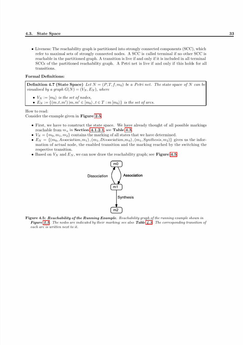
5.1.1 Examples . . . . . . . . . . . . . . . . . . . . . . . . . . . . . . . . . . . . . . . . 505.2 Continuous Petri Nets . . . . . . . . . . . . . . . . . . . . . . . . . . . . . . . . . . . . . 52
5.2.1 Examples . . . . . . . . . . . . . . . . . . . . . . . . . . . . . . . . . . . . . . . . 53
6 Model Checking for Petri Nets 556.1 Introduction to Model Checking . . . . . . . . . . . . . . . . . . . . . . . . . . . . . . . . 556.2 Temporal Logics . . . . . . . . . . . . . . . . . . . . . . . . . . . . . . . . . . . . . . . . 55
6.3 Analytical Model Checking . . . . . . . . . . . . . . . . . . . . . . . . . . . . . . . . . . 58
VII

8/15/2019 Bla Et Ke Tutorial
http://slidepdf.com/reader/full/bla-et-ke-tutorial 8/108
6.3.1 Computation Tree Logic (CTL) . . . . . . . . . . . . . . . . . . . . . . . . . . . . 586.3.2 Branching-time Continuous Stochastic Logic (CSL) . . . . . . . . . . . . . . . . . 61
6.3.3 Linear Time Logic (LTL) . . . . . . . . . . . . . . . . . . . . . . . . . . . . . . . 626.4 Simulative Model Checking . . . . . . . . . . . . . . . . . . . . . . . . . . . . . . . . . . 636.4.1 Probabilistic Linear Time Logic (PLTL) . . . . . . . . . . . . . . . . . . . . . . . 646.4.2 Continuous (Probablistic) Linear Time Logic (LTLc/PLTLc) . . . . . . . . . . . 67
7 Petri Net Editor: Snoopy 697.1 Editor Mode . . . . . . . . . . . . . . . . . . . . . . . . . . . . . . . . . . . . . . . . . . 707.2 Elements of the Stochastic Petri Net Class . . . . . . . . . . . . . . . . . . . . . . . . . . 71
7.2.1 Places . . . . . . . . . . . . . . . . . . . . . . . . . . . . . . . . . . . . . . . . . . 727.2.2 Transitions . . . . . . . . . . . . . . . . . . . . . . . . . . . . . . . . . . . . . . . 737.2.3 Edges . . . . . . . . . . . . . . . . . . . . . . . . . . . . . . . . . . . . . . . . . . 757.2.4 Parameters . . . . . . . . . . . . . . . . . . . . . . . . . . . . . . . . . . . . . . . 77
7.3 Configuration Sets . . . . . . . . . . . . . . . . . . . . . . . . . . . . . . . . . . . . . . . 77
7.4 Animation Mode . . . . . . . . . . . . . . . . . . . . . . . . . . . . . . . . . . . . . . . . 777.5 Simulation Mode . . . . . . . . . . . . . . . . . . . . . . . . . . . . . . . . . . . . . . . . 787.6 Model Checking Mode . . . . . . . . . . . . . . . . . . . . . . . . . . . . . . . . . . . . . 807.7 Get started . . . . . . . . . . . . . . . . . . . . . . . . . . . . . . . . . . . . . . . . . . . 82
7.7.1 Modelling . . . . . . . . . . . . . . . . . . . . . . . . . . . . . . . . . . . . . . . . 827.7.2 Simulation/Animation . . . . . . . . . . . . . . . . . . . . . . . . . . . . . . . . . 85
8 Petri Net Analyser: Charlie 878.1 Graphical User Interface . . . . . . . . . . . . . . . . . . . . . . . . . . . . . . . . . . . . 87
8.1.1 Marking Editor . . . . . . . . . . . . . . . . . . . . . . . . . . . . . . . . . . . . . 898.1.2 IM-based Analysis . . . . . . . . . . . . . . . . . . . . . . . . . . . . . . . . . . . 908.1.3 Siphon/Trap Computation . . . . . . . . . . . . . . . . . . . . . . . . . . . . . . 918.1.4 Reachability Graph/Coverability Graph . . . . . . . . . . . . . . . . . . . . . . . 928.1.5 Model Checking . . . . . . . . . . . . . . . . . . . . . . . . . . . . . . . . . . . . 948.1.6 Net Properties . . . . . . . . . . . . . . . . . . . . . . . . . . . . . . . . . . . . . 96
8.2 Visualisation of Analysis Results in Snoopy . . . . . . . . . . . . . . . . . . . . . . . . . 97

8/15/2019 Bla Et Ke Tutorial
http://slidepdf.com/reader/full/bla-et-ke-tutorial 9/108
CHAPTER 1Introduction
What is the background of this tutorial? During the last decade the integrative research areaof systems biology has been constantly gaining more importance. Experimental and computationalapproaches are combined to systematically investigate biological systems. To understand biology onits system level, the structural and dynamic properties of regulatory networks in biological systemshave to be represented by a model describing the involved species and their interactions. Petri nettheory offers the possibility to construct and analyse such models and to represent their structural anddynamic propertoies by various techniques.
Who should read this tutorial? This tutorial addresses scientists who are looking for an easy
and intuitive way to translate a biological system into a Petri net model at arbitrarily chosen level of abstraction with the option of representing time and/or space-dependent processes. The tutorial isequally suitable for experimental and theory oriented bio-scientists. The examples given in the tutorialcan be used by the interested reader to model her/his own biological system.
What can I learn? The tutorial offers an introduction to the Petri net formalism, how to construct amodel of a biological system, analyse its structure and dynamic behaviour in terms of time-dependentbehaviour, which is shown by several intuitive examples. At the end of the tutorial you will be able tomodel a biological system on your own using Petri nets. You will also know how to analyse the structureof your model, how to interpret the results and how to perform simulation studies to investigate thetime-dependent dynamic behaviour. In addition, we also provide a chapter about model checking,which might be helpful to evaluate your model by verifying specified properties that you are interestedin. We also show how to use the two Petri net tools Snoopy [19] and Charlie [8]. Based on these
instruments you will be able to enhance your knowledge about the modelled biological system and todraw new conclusions from that.
Why should I use Petri nets? The graphical notation and construction of Petri nets allows youto easily and intuitively construct models of biological systems and to characterize the structure,behavioural properties related to the structure and time-dependent dynamic behaviour of a model byseveral related techniques. Petri nets can describe concurrent and parallel processes, as well as commu-nication and synchronization in bipartite systems regardless of the abstraction level in a comprehensiveand mathematically correct model [12]. Time as well as space aspects can be modelled by a Petri net.Several specialized Petri net classes are available to describe different scenarios and to consider differentsimulative approaches. Therefore, the kinetics of the qualitative Petri net model can be considered asstochastic, continuous or as a mixture of both (hybrid) [12].
In silico experiments with Petri net models permit to systematically analyse a biological system by
1

8/15/2019 Bla Et Ke Tutorial
http://slidepdf.com/reader/full/bla-et-ke-tutorial 10/108
2 Introduction
applying structural as well as dynamic analysing techniques to investigate perturbations. From theobtained results new insights can be achieved about the biological system. Thereby, you can increase
your understanding, reveal gaps in knowledge, and detect missing and/or essential components. Basedon a valid model it is possible to predict the system behaviour. This is might be helpful to investigatepathological states and their molecular basis aimed at identifying potential targets to develop thera-peutical intervention strategies.The Petri net formalism offers quite a few advantages over other and more broadly used modellingframeworks.. The different Petri net classes are interconvertible with each other without changingthe qualitative structure. Due to the graphical visualisation of molecular networks by Petri nets, abioscientist can intuitively understand the modelled mechanisms. The user does not have to dealwith many different representations of a molecular network which do not obviously correspond to eachother like a biological cartoon, the structure of the biological network, the mathematical equations(stochastic, continuous, etc.) and the implementation of the equations. Besides, the transformationof a molecular network represented by an Petri net into e.g. ODE equations is unique, but not viceversa [24]. Several reliable analysis tools have been develop to investigate qualitative and quantitative
properties of Petri nets by structural analysis, simulation of the time-dependent dynamic behaviourand model checking.
What is the scheme of this tutorial? First of all, you will learn all the basics about the Petrinet formalism motivated by small biological examples that are easy to understand. Next, you will seehow to analyse the structure of a model and how to interpret the obtained results and their biologicalmeaning. Afterwards, you will learn how to perform simulations with your model. We also offer achapter about model checking, where you can learn how to verify specific properties of your model thatyou are interested in. Then, we introduce the two Petri net tools Snoopy [19] and Charlie [8].All sections, where theoretical concepts are explained, are divided into an informal and a formal part.We start with an informal introduction, where we explain the basics and the biological relations.Subsequently and to be complete, we give the formal definitions and a small help on “how to read” the
definitions at the end of the section.
What tools do I need? Several tools are available to model biological systems, simulate their time-dependent dynamic behaviour and analyse their structure. Here, we use the Petri net editor Snoopy [19]to model biological systems and simulate/animate their time-dependent dynamic behaviour. Charlie [8] is used to analyse the Petri net structure. Both software tools were developed at the chair of DataStructures and Software Dependability at the Brandenburg University of Technology Cottbus and arefreely available for non-commercial use. You can download them at http://www-dssz.informatik.
tu-cottbus.de/DSSZ/Software/Software [1].

8/15/2019 Bla Et Ke Tutorial
http://slidepdf.com/reader/full/bla-et-ke-tutorial 11/108
CHAPTER 2Petri Net Basics
In this chapter we give you all relevant information about Petri nets. We answer the questions:
What are Petri Nets?Why are Petri nets useful and efficient in modelling biological systems?How are Petri nets defined?
First of all, what does “Petri” mean?
“Petri nets are used as a formal and graphically appealing language which isappropriate for modelling systems with concurrency and resource sharing. Petri net
modelling has been under development since the beginning of the 60’ies, where Carl AdamPetri defined the language. It was the first time a general theory for discrete parallel
systems was formulated. The language is a generalization of automata theory such thatthe concept of concurrently occurring events can be expressed.” [2]
Figure 2.1: Carl Adam Petri. Carl Adam Petri (12 July 1926 – 2 July 2010) was a German mathematician and computer scientist. He was born in Leipzig. Petri nets were invented in August 1939 by Carl Adam Petri at at the age of 13 for the purpose of describing chemical processes. He documented the Petri net in 1962 as part of his dissertation, Kommunikation mit Automaten (communication with automata) [ 4] .
3

8/15/2019 Bla Et Ke Tutorial
http://slidepdf.com/reader/full/bla-et-ke-tutorial 12/108
4 Petri Net Basics
2.1 General Information about the use of Petri Nets in modeling
biological processes
Petri nets were originally designed to represent discrete, concurrent processes of technical systems. Theycombine an intuitive, unambiguous, qualitative bipartite graphical representation of arbitrary processeswith a formal semantics. Thus, the power of Petri nets is the explicit representation of concurrentprocesses, but they also offer a simple and flexible modelling language. Petri nets are also powerful anduseful in modelling biological systems. Petri nets may unambiguously represent (bio-)chemical reactionsin metabolism, signal transduction and gene expression and have been applied to neuronal processes aswell. In the biological context, Petri nets are especially efficient in reconstructing complex molecularnetworks. A Petri net may represent:
• Stochastic (discrete) and kinetic (continuous) processes at arbitrary resolution of molecular detailwithin a single, coherent model;
• any chemical or biochemical reaction at any resolution of kinetic detail,
• the localization of molecules in different spatial compartments (cytoplasm, nucleus, etc.), as wellas different localization in 1-, 2- or 3- dimensional space, and the translocation between differentlocations;
• the signalling states of single molecules, circuits or networks,• the physiological state, behaviour or response of a cell.
Petri nets have already been applied to biological case studies like the regulation of the lac operon[21], Duchenne muscular dystrophy [10], the response of S. cerevisiae to copulatory hormones [7] and theyeast cycle [18]. Two examples for Petri nets applied to metabolic systems are the sucrose breakdownpathway in the potato tuber [13] and the iron homoeostasis process in human body [20]. There are alot of other interesting articles dealing the application of Petri nets to biological systems, which can notall be cited. The abstraction degree of a model can vary from single molecules to cells to multicellularaggregations. Even a whole organism or population can be described by a Petri net. A Petri net canalways be extended or edited by refining the components of the model by subnets. Advantageously,missing qualitative or kinetic information can be handled by Petri nets. The iterative process betweenwet-lab experiment and model-based predictions enables the researcher to close such gaps.
Figure 2.2: Conceptual Framework. The Petri net formalism allows to switch between different network classes to describe qualitative (QPN), stochastic (SPN) and continuous (CPN) information in a cohesive Petri net model [12] .
Petri nets may serve as umbrella formalism to integrate qualitative and quantitative modelling,which allows to apply various analysis techniques. Several reliable software tools, which support thePetri net formalism are developed by the international community on computational methods [19].Several specialized Petri net classes like qualitative, stochastic, continuous, or hybrid Petri nets and theircoloured counterparts are available to describe different scenarios and to consider different simulativeapproaches. All network classes are interconvertible with each other without changing the networkstructure; see Figure 2.2. This allows the application of the same powerful analysis techniques to the
underlying qualitative structure of all Petri net classes [12]. The wide range of network classes allows

8/15/2019 Bla Et Ke Tutorial
http://slidepdf.com/reader/full/bla-et-ke-tutorial 13/108
2.2. Standard Petri Net 5
the integration of qualitative, continuous and stochastic information. This allows the representationof different kinetic processes and different data types. Petri nets link structural and dynamic analysis
techniques to investigate and validate a model such as graph theory, application of linear algebra tocheck a model and simulation methods. This facilitates the performance of simulation studies to explorethe time-dependent dynamic behaviour, the in-depth analysis of structural criteria and the state spaceof a model.
2.2 Standard Petri Net
A Petri net is represented by a directed, finite, bipartite graph, typically without isolated nodes. Thefour main components of a general Petri net are: places, transitions, arcs and tokens; see Figure 2.3,A.
Figure 2.3: Petri Net Formalism. Petri nets consist of places, transitions, arcs and tokens (A). Just places are allowed to carry tokens (B). Two nodes of the same type can not be connected with each other
(C). The Petri net represents the chemical reaction of the water formation (D). A transition is enabled and may fire if its pre-places are sufficiently marked by tokens.
Places are passive nodes. They are indicated by circles and refer to conditions or states. In abiological context, places may represent: populations, species, organisms, multicellular complexes,single cells, proteins (enzymes, receptors, transporters, etc.), molecules or ions. But places could alsoembody temperature, pH-value or membrane potential; see also Section 3.3.1. Only places are allowedto carry tokens; see Figure 2.3, B.
Tokens are variable elements of a Petri net. They are indicated as dots or numbers within a placeand represent the discrete value of a condition. Tokens are consumed and produced by transitions; seeFigure 2.3, D. In biological systems tokens refer to a concentration level or a discrete number of a
species, e.g., proteins, ions, organic and inorganic molecules. Tokens might also represent the value of physical quantities like temperature, pH value or membrane voltage that effect biological systems. APetri net without any tokens is called “empty”. The initial marking affects many properties of a Petrinet, which are considered in Chapter 2.
Transitions are active nodes and are depicted by squares. They describe state shifts, system eventsand activities in a network. In a biological context, transitions refer to (bio-)chemical reactions,molecular interactions or intramolecular changes; see also Section 3.3.1. If a place is connected byan arc with a transition, the place (transition) is called pre-place (post-transition). If a transitionis connected by an arc with a place, the transition (place) is called pre-transition (post-place); seeFigure 2.4. Transitions consume tokens from its pre-places and produce tokens within its post-placesaccording to the arc weights; see Figure 2.3, D.

8/15/2019 Bla Et Ke Tutorial
http://slidepdf.com/reader/full/bla-et-ke-tutorial 14/108
6 Petri Net Basics
Figure 2.4: Places and Transitions. Place p1 is called pre-place of transition t1, and transition t1 is the post-transition of place p1. Place p2 is called post-place of transition t2, and transition t2 is the pre-transition of place p2.
Directed arcs are inactive elements and are visualised by arrows. They specify the causal relation-ships between transitions and places and indicate how the marking is changed by firing of a transition.Thus, arcs define reactants/substrates and products of a (bio-)chemical reaction. Arcs connect onlynodes of different types; see Figure 2.3, C. Each arc is connected with an arc weight. The arc weightsets the number of tokens that are consumed or produced by a transition. The stoichiometry of a(bio-)chemical reaction can be represented by the arc weights.
The Petri net Semantic describes the behaviour of the net, which is defined by firing rulesconsisting of a precondition and the firing itself. The firing of a transition depends on the markingof its pre-places. A transition is enabled and may fire, if all pre-places are sufficiently marked. If a transition has no pre-places it is always enabled to fire. By firing a transition moves tokens frompreplaces to postplaces and possibly changes the number of tokens. The firing of a transition changesthe marking of the connected places. Thus, the marking of the net is changed to a new reachablemarking, where some transitions are not any more enabled while others get enabled. The behaviour of a net is established by repeated firing of transitions. All possible ordered firing sequences result intothe whole net behaviour, which is also called state space.
Formal Definitions:
Definition 2.1 (Standard Petri net) A standard Petri net is a quadruple N = (P, T, f, m 0),
where:
• P, T are finite, non-empty, disjoint sets. P is the set of places. T is the set of transitions.• f: ((P × T) ∪ (T × P)) → N0 defines the set of directed arcs, weighted by non-negative integer
values.• m 0: P → N0 gives the initial marking.
How to read:Assume the following small example of an enzymatic reaction; see Figure 2.5:
Figure 2.5: Running Example. To illustrate the definition, we use the example of an enzymatic reaction A + E ↔ AE → E + B.
The Petri net N = (P , T , f , m0) in our running example; see Figure 2.5, consists of places P ,
transitions t, directed arcs f and the initial marking m0:

8/15/2019 Bla Et Ke Tutorial
http://slidepdf.com/reader/full/bla-et-ke-tutorial 15/108
2.2. Standard Petri Net 7
• Set of places P : P = {Enzyme, Substrate, EnymeSubstrateComplex, P roduct}• Set of places T : T = {Association, Dissociation, Synthesis}
• Set of directed arcs: ((P × T ) ∪ (T × P )) is the combination of the following subsets– Places connected with (→) transitions:
(P × T ) = {Substrate × Association,
Enymze × Assoication,
EnymeSubstrateComplex × Dissociation,
EnymeSubstrateComplex × Synthesis}
– Transitions connected with (→) places:
(T × P ) = {Assoication × EnymeSubstrateComplex,
Dissociation × Substrate,
Dissociation × Product,Synthesis × Product,
Synthesis × Enzyme}
• Initial Marking m0: m0 = {Enzyme = 1, Substrate = 1, EnymeSubstrateComplex = 0,Product = 0};the amount of tokens must be expressed as an integer variable.
At this point, we also like to introduce further notions and notations, which we use during thetutorial. The notation m( p) refers to the number of tokens on place p in the marking m. Place p isclean (empty, unmarked) in m if m( p) = 0, otherwise place p is clean (empty, unmarked) in m. A setof places is called clean if all places are clean, otherwise the set is marked. The postset and preset of anode x ∈ P ∪ T , is defined as:
• Preset: •x := {y ∈ P ∪ T | f (y, x) = 0}• Postset: x• := {y ∈ P ∪ T | f (x, y) = 0}
For places and transitions, we get four types of sets:
• •t - preplaces of transition t (reaction’s precursor)• t• - postplaces of transition t (reaction’s products)• • p - pretransitions of place p (all producing reactions of a component)• p• - posttransitions of place p (all consuming reactions of a component)
This definition can be extended and generalized for a set of nodes X ⊆∈ P ∪T . Now, the set of prenodesis given by •X :=
x∈X •x and the set of postnodes refers to X • :=
x∈X •x
Definition 2.2 (Firing Rule) Let N = (P, T, f, m 0) be a Petri net:
• A transition is enabled in marking m, written as m [t, if ∀ p ∈ •t : m( p) ≥ f ( p, t), else disabled.• A transition t, which is enabled in m, may fire.• When t in m fires, a new marking m is reached, written as m [t m, with ∀ p ∈ P : m( p) =
m( p) − f ( p, t) + f (t, p).• The firing happens atomically and does not consume any time.
How to read:Assume the example above; see Figure 2.5:
• The transition Association is enabled in marking m0 = (1, 1, 0, 0), because the marking of bothpre-places (Enzyme = 1, Substrate = 1) of the transition Assoiciation are equal to the respective
arc weight (in both caes “1”).

8/15/2019 Bla Et Ke Tutorial
http://slidepdf.com/reader/full/bla-et-ke-tutorial 16/108
8 Petri Net Basics
• Thus, the enabled transition Association may fire in m0.• Firing of the transition Association in m0, leads to the marking m1 = (0, 0, 1, 0). The transition
Assoication removes one token from the place Enzyme and one token from the places Substrate,both places do not get back any tokens. In consequence, both places are empty. The placeEnzymeSubstrateComplex gains one new token. The place Product is not involved and thus,the number of tokens is not changed at all.
In addition, m ∈ N|P |0 defined the marking of the given token situation, whereby |P | denotes the
number of places in a Petri net. All markings, which can be reached from a given marking m by anyfiring sequence, form the set of reachable markings [m. The set of markings [m0 reachable from theinitial marking m0 constitutes the state space of a model.
2.3 Extended Standard Petri Net
2.3.1 Extended Representation
For representationals reason of large networks two more specific types of nodes (transitions, places) havebeen developed, called logical nodes and macro nodes. Both types allow to neatly arrange networks, butdo not affect the properties of the Petri net. Indeed, this nodes are very useful to represent biologicalsystems
• Logical nodes : A logical transition or places is indicated by a slight grey shade; see Figure2.6. Logical nodes can be used to represent frequent elements in a network by identical copiesof a node, e.g., reactions or components. Thus, logical nodes are a kind of connectors bringingtogether identical nodes that are repeated in the network structure. Logical places can be used torepresent components with many cross links, like second messengers (cAMP, DAG, IP3 etc.), orenergy equivalents (ATP, NADH etc.) that are linked to numerous reactions. Logical transitionare able to represent reactions that are repeated all over the network or reaction, where a lot of
components are involved. Such a reaction can be split in single parts using logical transitions.
Figure 2.6: Logical Nodes. Two representations of a reaction using logical places (A) and logical transitions (B). The reaction A + E ↔ AE → E + B is split in single blocks. In (A) this blocks are chosen according the reaction, substrates and products are represented as logical places. In (B) each block represents al l reactions that are related to the respective components. Here logical transitions are used.
• Macro nodes : A macro node or a macro place are visualised as boxed nodes; see Figure 2.7.
Macro nodes allow to hierarchically structure a network. Each macro node establish a new layer

8/15/2019 Bla Et Ke Tutorial
http://slidepdf.com/reader/full/bla-et-ke-tutorial 17/108
2.3. Extended Standard Petri Net 9
of the network. Macro nodes can be arbitrarily nested. Advantegeously, macro nodes offer thepossibility to refine the network structure on a new layer. In addition, macro nodes also allow
to structure a model into meaningful parts of connected subnets, group species or reactions oradapted the hierarchical structure of biological networks, e.g., compartmentalization of cells or anentire organism. The boundary nodes of a macro place are transitions. Macro transitions haveonly boundary places.
Figure 2.7: Macro Nodes. Macro nodes allow refining of places or transitions by a detailed subnets on a deeper hierarchical level. The border nodes of a macro transition (place) are places (transitions).
2.3.2 Extended Expressiveness
In order to reinforce the expressiveness of Petri nets, two arc types have been introduced, read (or test)edge and inhibitor edge; see Figure 2.8. Both types of arcs can be used to easier represent certainrelationships in the network.
Figure 2.8: Inhibitor Edge and Read Edge. (A) Read edge: Transition t1 is enabled if place A and B are sufficiently marked. After firing, tokens are deleted from place B, but not from place A, which is connected with transition t1 by a read edge. (B) Inhibitor edge: Transition t1 is enabled if place B is sufficiently marked and place A is not sufficiently marked, which is connected with transition t1 by an inhibitor edge.After firing tokens are deleted from place B, but not from A.

8/15/2019 Bla Et Ke Tutorial
http://slidepdf.com/reader/full/bla-et-ke-tutorial 18/108
10 Petri Net Basics
• Read edges are represented by an edge and a filled dot at its end. Read edges only connect aplace with a transition. If a place p is connected with a transition t via a read edge, the transition
t is enabled if place p and all other places connected with transition t via the standard arc aresufficiently marked. By firing transition t, the amount of tokens on place p is not changed. Readedges can also be adapted by two opposed standard arcs. Thus, the qualitative analysis techniquesof Petri nets can also be applied to models containing read edges.
• Inhibitor edge are represented by an edge and an empty dot at the end. Inhibitor edges onlyconnect places with transitions. If a place p is connected with a transition by an inhibitor edge,the transition t is enabled if place p is not sufficiently marked, meaning the amount of tokensmust be less than the respective arc weight, and all other places connected with transition t viathe standard arc are sufficiently marked. Tokens are not deleted from the place p if the transitiont fires. Inhibitor edges can not be reduced to the standard edges and thus they cause radicalmodification. All here introduced qualitative analysis techniques are not applicable to modelscontaining inhibitor edges.

8/15/2019 Bla Et Ke Tutorial
http://slidepdf.com/reader/full/bla-et-ke-tutorial 19/108
CHAPTER 3Petri Net Modelling
After the theoretical excursion, we now address the modelling procedure itself. Here, we answer thefollowing questions:
What is a model?What can you expect from your model?What points need to be considered before modelling?How can you create your own Petri net model?
Modelling a biological system is similar to designing a game board. In both cases you need to defineits structure and therewith the actions that are allowed and the different states that can be reached by
each action.
First of all, you need to be aware that a model is only a simple, abstract representation of reality. Amodel can not explain every detail of the real biological system, but a model can help you to understandthe structural relationships and the time-dependent dynamic behaviour. You can not expect newinformation about your biological system that you have not indirectly defined in the network structureand in the kinetics of the model. But do not be afraid if you do not have all detailed information of thebiological system (components, reactions, kinetics) that you want to model. Even in this case, a modelcan be very helpful in studying the behaviour of the model or in revealing missing components andreactions. Even more, a model might also help to estimate kinetic parameters. This can be done bytesting various modifications and perturbations, which would never be possible in your real system orwould be too expensive. You may be able to test any hypotheses about the biological system by makingmodel predictions. Additionally, in the case of Petri net models, there are several reliable analysis
techniques available which might help you to better understand your model.In the following sections, we talk about all steps that you need to consider while creating a qualitativemodel. After constructing your model, you can analyse its structure and the time-dependent dynamicbehaviour. These two options are discussed in Chapter 4 and 5.
3.1 Analysing the System of Interest
Before starting the modelling procedure itself, you have to analyse your system very carefully and thinkabout the points listed below.
1. Step: Make assumptions and think about abstractions to keep your model as simple as possible.2. Step: Set boundaries to reasonably limit your model.
3. Step: Identify the involved components (and perhaps their different states).
11

8/15/2019 Bla Et Ke Tutorial
http://slidepdf.com/reader/full/bla-et-ke-tutorial 20/108
12 Petri Net Modelling
4. Step: Identify all actions, (bio-)chemical reactions and any other changes occurring in your system.5. Step: Define the relationships between components and reactions.
6. Step: Define the stoichiometry.7. Step: Define the initial state.
Ask yourself what you know about the biological system. Perhaps, you have to go to the literatureand collect more information about the components and reactions that are involved in your system. Youshould decide what the model should reflect and in how much detail you want to describe your system.Think of reasonable boundaries and of suitable assumptions to restrict the model of the biologicalsystem. A model should always be self-contained and as simple as possible. Often, it is not necessaryto describe everything in detail. Start with a simple model. You can always refine your model and addfurther information if necessary.
3.2 Assumptions and Modelling Guidelines
Before modelling you should think of reasonable boundaries and of suitable assumptions to restrictthe model of the biological system. But it is also important to agree on a conformable modellingprocedure. All three points are important requirements to create a consistent model and to avoiderrors, inconsistencies and contradictions while modelling.
Assumptions directly related to the biological context depend on the current issue and the chosenabstraction level. Therefore, you have to think about:
• System boundaries:include all relevant components and reactions;• Abstraction level of processes: consider reactions in detail or merge a set of reactions into one
bigger step;• Abstraction level of the involved components: consider components as on unit, consider different
states of a component or consider even functional domains of components;• Handling of non-limiting components: “pseudo reactions” could be used to independently produce
such components;• Handling of products that have no more function in a model: “pseudo reactions” could be used
to remove such components;• Space: consider different compartments of the biological system and the translocation of compo-
nents or neglect spatial information.
Additional scenarios are conceivable to model a biological system depending on the special context.
The decision on the modelling guideline goes along with the preassigned assumptions and boundaries.Here, we suggest some useful guidelines that you can consider while modelling. The strict observancedepends also on the given issue, available information and chosen abstraction level.
The following guidelines are suitable for modelling biological systems:
• Reaction pathways (= Sequence of reactions reproducing its initial state, see also T-invariants,Section 4.2.3) like signal cascades or metabolic routes cover the entire model to restore the initialstate of the model.
• The constant sum of molecules belonging to related components or different states of a componentmust be preserved (=Sum of tokens over a set of place is constant, see also P-invariants, Section4.2.3). Mass conservation is assured if this property holds for each component (place) in themodel.
• A Petri net model should be transition-bordered (all places have pre- and post-transitions), orplace-bordered (all transitions have pre- and post-places), or not contain any border nodes at all(closed network structure).
– Use input transitions to ensure that substrates do not limit the internal processes in a model.

8/15/2019 Bla Et Ke Tutorial
http://slidepdf.com/reader/full/bla-et-ke-tutorial 21/108
3.3. Creating a Petri Net Model 13
Figure 3.1: Representation of Enzymatic Reactions: Petri net shown in (A) refers to a simple
annotation of an enzymatic reaction S
E
→ P. We couple the enzyme with the reaction by a read edge.Thereby the enzyme does not get consumed. The Petri net in (B) illustrates the single steps of an enzymatic reaction S + E → ES → EP → P + E. The enzyme is temporarily consumed, but at the end released again.
– Use output transitions to ensure that products do not infinitely increase.– Use input places to ensure that initial substrates limit internal processes in the model.– Use output places to ensure that products accumulate.
• High abstraction level:
– Reactions triggered by a component or a specific condition (temperature, pH value, mem-brane voltage) are considered as one single simplified reaction. Enzymes and similar triggersare not consumed by the reaction. They are connected with the corresponding transition via
a read edge; see Figure 3.1, A.– A reaction sequence is reduced to one step.
• Low abstraction level:
– Enzymatic reactions are refined into subreactions; see Figure 3.1, B.– Each reaction is split into elementary steps.
3.3 Creating a Petri Net Model
To construct a Petri net model of a biological system, the involved reactions and components mustbe identified according to the assumptions and the modelling guidelines in the step before. You needto represent all reactions as transitions. Places represent specific conditions (temperature, membranevoltage, pH-Value) or components. Afterwards you need to define the relationships between placesand transitions with the help of arcs, and the stoichiometry by arc weights. Section 3.6 gives severalexamples of how to translate chemical and enzymatic reactions into Petri nets.
3.3.1 Biological Interpretation of Places and Transition
In this section, we summarize biological interpretations of places and transitions. Both list are notcomplete and you can always add your own interpretation depending on your biological system.A place could represent:
• molecular level:
– atoms,
– ions,

8/15/2019 Bla Et Ke Tutorial
http://slidepdf.com/reader/full/bla-et-ke-tutorial 22/108
14 Petri Net Modelling
– small inorganic molecules (oxygen, water, carbon dioxide, phosphates, acids, bases, etc.),– small organic molecules ( hydrocarbons, carbohydrates, nucleic acid, amino acids, etc.),
– second messengers (cAMP, DAP, IP3, PIP2, etc.),– energy equivalents (ATP/ADP, GTP/GDP, NAD+/NADH, NADP+/NADPH, etc.),– proteins (enzymes, transporter, ion-channels, protein complexes, protein domains, etc.),– molecules in certain localisations
• cellular level:
– specific cell types (epidermal cells, neurons, germ cells, blood cells, etc.),– state of a single cell (healthy, infected, diseased, etc.),– single cell organism (bacteria, virus, etc.),– compartment of a cell (nucleus, endoplasmic reticulum, lysosome, mitochondria, etc.),– structural component of a cell (membrane, DNA, ribosome, cytoplasm, etc.)
• multicellular level:
– cell complexes (layer of identical, different cells, etc.),
– tissue (muscles tissue, nervous tissue, epithelial tissue, etc.),– organs (skin, muscles, liver, lunges, etc.),– multicellular organism (human, animal, plants, fungi, etc.),– populations (single-cell organisms, multicellular organisms, etc.),– state of the multicellular complex (healthy, infected, diseased, etc.),
• non-biological factors:
– environmental factors (sun, wind, food, stress, etc.),– physical properties (pH-value, temperature, membrane voltage, pressure, red light, etc.),– abstract factors or conditions.
If you think of transitions, they can be interpreted as:
• (bio-)chemical reaction,• dissociation/association,• state shifts,• actions,• molecular changes,• transport (active, inactive)/diffusion,• phosphorylation/dephosphorylation,• translation/transcription,• degradation/synthesis,• any event related to the above mentioned interpretation of places.
To keep this tutorial as simple as possible, we generalize the interpretation of places to componentsand the interpretation of transitions to reaction.
3.3.2 Petri Net Models of Biomolecular Reactions
Among the biological systems, a lot of similar processes are involved and in addition processes can becategorised by their functionality. Biological processes of one group can be simplified to a generalizedmechanism. Here, we summarize such generalized mechanisms that you can find very frequently inbiological systems. For each of those examples, we provide the Petri net structure of and small biologicalcartoon. You can reuse the Petri net models in your own model and connect different submodels witheach other. The first Figure 3.2 shows typical chemical reactions and their corresponding Petri netstructure. Figure 3.3, we consider different transport mechanisms and how to represent them bya Petri net. Some Petri nets of general mechanisms in signal transduction are given in Figure 3.4.Posttranslational modifications (PTMs) regulate the functionality and activity of proteins and are thus,important in many biological mechanisms. Figure 3.5 shows generalized Petri net models of the most
common PTMs.

8/15/2019 Bla Et Ke Tutorial
http://slidepdf.com/reader/full/bla-et-ke-tutorial 23/108
3.3. Creating a Petri Net Model 15
Figure 3.2: Chemical Reactions.
Here we depict Petri net structures of typical chemical reactions (adopted from [ 17].
Figure 3.3: Molecular Transport Mechanisms. Molecular Transport Mechanisms translated into Petri net models.

8/15/2019 Bla Et Ke Tutorial
http://slidepdf.com/reader/full/bla-et-ke-tutorial 24/108
16 Petri Net Modelling
Figure 3.4: Signalling Mechanisms. Most common signalling mechanisms translated into Petri net models (adopted from [ 15 ]).

8/15/2019 Bla Et Ke Tutorial
http://slidepdf.com/reader/full/bla-et-ke-tutorial 25/108
3.3. Creating a Petri Net Model 17
Figure 3.5: Posttranslational modification. Posttranslational modifications(PTMs) of proteins translated into Petri net models.

8/15/2019 Bla Et Ke Tutorial
http://slidepdf.com/reader/full/bla-et-ke-tutorial 26/108
18 Petri Net Modelling
3.4 Initial State of a Petri Net Model
After setting the network structure of the Petri net, its initial state has to be defined, e.g., accordingto the initial state of the biological system. It is not necessary to put tokens on every single place. Toset the initial marking you have to consider the following points:
• What is your input (substrates, signals)?• Which internal components are available at the beginning?• Which is the initial state of a component?• Which are the structural components in your system (membranes, compartments, cell organells,
DNA etc.)?
Another way to set an initial marking is to consider P-invariants; see Section 4.2.3. Every P-invariant should be initially marked by a token. The reactions in your model can only occur (transitionscan only fire) if places are sufficiently marked. Thus, the initial marking determines the state spaces,
meaning which states can be reached. With the help of the initial marking you can also simulatelimitation, knock-downs or knock-outs and mutations or overexpression. You can test the influence of different manipulations and perturbations in your model on general and behavioural network properties,the state space and time-dependent dynamic behaviour.
3.5 Neat Arrangement of a Petri Net Model
Sometimes the network structure of a biological system grows very fast and the reflected processes arevery complex. Additionally, in biological networks some components are highly interactive and act atseveral reactions, like second messenger and energy equivalents. Thus, the model might not be veryreadable, but confusing. To enhance the readability of your model you can use macro nodes and logicalnodes if necessary; see Section 2.2, Figure 2.7.
Figure 3.6: Joining Submodels. Macro nodes can be used to build neatly arranged and hierarchically structured submodels. Separate submodels can be coupled by logical places that refer to the same component
in all submodels.
The application of macro nodes leads to a hierarchical model with different levels that are connectedwith each other. Hierarchical models allow you to neatly display the network structure. The hierarchicalstructure of a model does not change any properties of the flat model. With the help of macro nodesyou can refine single places or transitions by a detailed subnet on a lower level and/or you can organizeyour model into functional units. A model could be subdivided into reaction sets, signal cascades orrelated components. To represent highly cross-linked components and transitions with multiple inputand output, you should consider using logical places and transitions. By using macro nodes and logicalplaces you can construct separate Petri net models and join them afterwards; see Figure 3.6. Thesubmodels are connected via logical places, i.e., places of components that are shared among differentsubmodels. The construction and analysis of separate Petri net models might also avoid errors and
inconsistencies.

8/15/2019 Bla Et Ke Tutorial
http://slidepdf.com/reader/full/bla-et-ke-tutorial 27/108
3.6. Examples 19
3.6 Examples
The next pages more examples of different enzymatic reactions like enzyme inhibition, signal amplifi-cation, feedback inhibition and gene regulation. As before in Section 3.3.2, these general structurescan be reused in any biological system.
Example 3.1 (Enzymatic Reaction) Here are two possibilities showing how to represent an enzy-matic reaction using Petri nets. In A, the enzymatic reaction is simplified to one reaction. In B , we consider in addition the formation of an enzyme-substrate-complex. The enzymatic reaction is split intotwo steps.
Example 3.2 (Enzymatic Reaction Coupled with Gene Expression) The simple enzymatic reaction in A can be extended by adding more and more details about the gene expression, see B and C .

8/15/2019 Bla Et Ke Tutorial
http://slidepdf.com/reader/full/bla-et-ke-tutorial 28/108
20 Petri Net Modelling
Example 3.3 (Feedback Inhibition) In this example, the negative feedback is initiated by the prod-uct that inhibits the first enzyme of the reaction sequence. To realise the inhibition the product is
connected with the first transition of the sequence via an inhibitor edge.
Example 3.4 (Signal Amplification) In signal amplification multiple enzymes activate each other step by step. Signal amplification can be found in different signal pathway, e.g., in the mitogen-activated protein kinase (MAPK) cascade, where each enzyme can activate several enzymes in the next step of the signal pathway.

8/15/2019 Bla Et Ke Tutorial
http://slidepdf.com/reader/full/bla-et-ke-tutorial 29/108
3.6. Examples 21
Example 3.5 (Competitive Enzyme Inhibition) The substrate and the inhibitor can both bind tothe active site of the enzyme. The inhibitor and substrate can not bind at the same time to the enzyme,
they exclude each other.
Example 3.6 (Allosteric Enzyme Inhibition) The inhibitor binds to a distinct site at the enzyme.Thus, the inhibitor does not compete with the substrate and can inhibit the enzyme independently whether the substrate is bound or not.

8/15/2019 Bla Et Ke Tutorial
http://slidepdf.com/reader/full/bla-et-ke-tutorial 30/108

8/15/2019 Bla Et Ke Tutorial
http://slidepdf.com/reader/full/bla-et-ke-tutorial 31/108
CHAPTER 4Qualitative Petri Net Analysis
In this chapter we talk about qualitative properties of the network structure and their meanings. Alldefinitions and classifications are taken from reference [12]. Also, consider reference [12] if you areinterested in more mathematical details. Here, we answer the questions:
Which properties can be determined for a Petri net model?What does each property mean in general?And what is the biological meaning of each property?Which are important components?How do I know, if my system can reach a certain state?
Again, the game board is a nice analogy to the modelling of a biological system. Each game hascertain structures and rules. It is not possible to play chess on a merels boards, or vice versa. The sameapplies for biological systems. Each biological system has defined properties that should be reflectedby its model.
The Petri net formalism allows you to characterize elementary system properties of the underlyingPetri net model. Those properties can be determined without considering kinetic information and,therefore, without considering the the the time-dependent dynamic behaviour. It is not just possible tomake statements about the pure qualitative properties of the network structure. The network structuresalso allows you to draw conclusions about behavioural properties independent of time of the model.The fulfilment of certain properties is important for the consistency and strict observance of rules
important for a biological system. These properties may vary among different case studies and dependon the specific issue, assumptions and modelling guideline. However, the properties of a Petri net canbe used to validate the model and to check relevant system properties. Each property has a significantbiological meaning.
4.1 Qualitative Properties
4.1.1 Structural Properties
The structural properties given in Table 4.1 are elementary properties of a Petri net graph, whichdirectly depend on the arrangement of places, transitions and arcs (including arc weights). Those prop-erties characterize the network structure and are independent of the marking. They can be considered
as an initial consistency check to prove that the model adheres to the assumptions and the modelling
23

8/15/2019 Bla Et Ke Tutorial
http://slidepdf.com/reader/full/bla-et-ke-tutorial 32/108
24 Qualitative Petri Net Analysis
guideline. Next to the informal description of each of those behavioural properties, we give the biologicalinterpretation.
Table 4.1: Qualitative Properties of a Petri net and their biological Meaning
Property Informal Definition Biological Meaning
PUR Pure There are no two nodes, directlyconnected in both directions. Thisprecludes read arcs and double arcs.
No component is produced and con-sumed by the same reaction. Thus,enzymatic or enzyme-like reactionsare formulated in more detail.
ORD Ordinary All arc weights are equal to 1. Every stoichiometric coefficient of each reaction is equal to one.
HOM Homogeneous All outgoing arcs of a given placehave the same multiplicity.
Each consuming reaction associatedwith one component takes the sameamount of molecules of this compo-
nent.CON Connected A Petri net is connected if it holds
for every two nodes a and b thatthere is an undirected path betweena and b. Disconnected parts of a Petri net can not influence eachother, so they can be usually anal-ysed separately. In the following weonly consider connected Petri nets.
All components in a system are di-rectly or indirectly connected witheach other through a set of reac-tions, e.g., metabolic paths, signalflows.
SC Strongly Con-nected
A Petri net is strongly connected if it holds for every two nodes a and bthat there is a directed path from a
to b, vice versa. Strong connected-ness involves connectedness and theabsence of boundary nodes. It is anecessary condition for a Petri netto be live and bounded at the sametime.
All components in a system are di-rectly connected with each otherthrough a set of reactions, e.g.,
metabolic paths, signal flows.
NBM Non-blockingMultiplicity
The minimum of the multiplicity of the incoming arcs for a place is notless than the maximum of the mul-tiplicities of its outgoing arcs.
The amount of produced and con-sumed molecules of a certain com-ponent is always equal.
CSV Conservative All transitions add exactly asmany tokens to their post-places as
they subtract from their pre-places(token-preservingly firing). A con-servative Petri net is structurallybounded.
The total amount of consumed andproduced molecules by a certain re-
action is always equal.
SCF Static conflictfree
There are no two transitions sharinga pre-place. Transitions involved ina dynamic conflict compete for thetokens on shared places.
For every reactant exist just onepossible reaction or there are no tworeactions sharing at least one reac-tant.
FT0 No input transi-tion
There exist no transitions withoutpre-places.
Infinite source of a component.
TF0 No output tran-sition
There exist no transitions withoutpost-places.
Sink of a component.

8/15/2019 Bla Et Ke Tutorial
http://slidepdf.com/reader/full/bla-et-ke-tutorial 33/108
4.1. Qualitative Properties 25
FP0 No input place There exist no places without pre-transitions.
The component can not be producedby any reaction. Thus, such compo-
nents are limiting.PF0 No output place There exist no places without post-
transitionsComponents can infinitely accumu-late in the system. Thus, they arenot consumed by any reaction.
4.1.2 Behavioural Properties
Behavioural properties of a Petri net are listed in Table 4.2 and 4.4; they characterize the systembehaviour of a model, which depend on the qualitative network structure and on the initial marking.The listed behavioural properties are independent of the time-dependent dynamic behaviour and thus,independent of kinetic information. Therefore, behavioural properties of a Petri net are determined bytime-free decision about the systems behaviour, meaning time aspects are not considered. Next to the
informal description of the behavioural properties, we give the biological interpretation.
4.1.2.1 General Behavioural Properties
General behavioural properties as shown in Table 4.2 illustrate the properties of a Petri net model char-acterizing the boundedness, liveness and reversibility based on the underlying network structure. Theseproperties are independent of the special functionality of the network itself. The informal definitions of the named properties are given below:
• Boundedness : For every place it holds that: Whatever happens, the maximum number of tokenson this place is bounded by a constant. This precludes overflow by unlimited increase of tokens;see 1-B, k-B, SB in Table 4.2.
• Liveness : For every transition it holds that: Whatever happens, it will always be possible to reach
a state where this transition gets enabled. In a live net all transitions are able to contribute tothe net behaviour forever, which precludes dead states, i.e., states where none of the transitionsare enabled; see also Liv, DSt, DTr in Table 4.2.
• Reversibility : For every state it holds that: Whatever happens, the net will always be able toreach this state again. So the net has the capability of self-reinitialization; see also REV in Table4.2.
The biological interpretation of those properties is given in Table 4.2.
Table 4.2: General Behavioural Properties of a Petri net and their biological Meaning
Property Informal Definition Biological Meaning
SB Structurally
bounded
A Petri is structurally bounded if it
is bounded in any initial marking.
It is not possible that any compo-
nent accumulates in the system in-dependent of the initial conditions.
1-B 1-bounded A Petri net is 1-bounded if all itsplaces are 1-bounded.
Number of molecules or the concen-tration of every component is lim-ited to one only.
k-B k-bounded A Petri net is k-bounded if all itsplaces are k-bounded.
Number of molecules or the concen-tration level of each component islimited to a constant number k.
LIV Liveness Every transition of a Petri net con-tributes to the network behaviourforever.
All involved reaction will repeatedlyoccur and contribute to the time-(and spatial-) dependent develop-ment.

8/15/2019 Bla Et Ke Tutorial
http://slidepdf.com/reader/full/bla-et-ke-tutorial 34/108
26 Qualitative Petri Net Analysis
REV Reversibility The initial marking can be reachedagain from each reachable marking.
The initial state of a system canbe reproduced by any possible state
reached from the initial conditions.DCF Dynamically
conflict freeA Petri net is has no dynamic con-flicts if no state exists, in which twotransitions are enabled, which coulddisable each other by firing.
The occurrence of a reaction inhibitsanother reaction which could alsooccur at the same time. The sharedreactants are consumed by one of the reaction and no reactants are leftor one reaction produces a compo-nent that directly inhibits the otherreaction.
DSt Dead states A Petri net has a dead state if notransition can be enabled any more.
The system can run into a state,where no reaction can occur.
DTr Dead transition A transition in a Petri net is dead if
it can not be enabled in any markingreachable from the initial marking.
The system can run from the initial
state chosen initial state into at leastone state, where at least one reac-tion can not occur any more.
Formal Definitions:
Definition 4.1 (Boundedness)
• A place p is k-bounded if there exists a positive integer number k, which represents an upper bound for the number of tokens on this place in all reachable markings of the Petri net:∃k ∈ N0 : ∀m ∈ [m0 : m ( p) ≤ k.
• A Petri net is k-bounded if all its places are k-bounded.• A Petri net is structurally bounded if it is bounded in any initial marking.
How to read:Please consider the example given in Figure 2.5. First, we need to consider all marking m reachablefrom the initial marking m0 by simply playing the token game. As result we get:
Table 4.3: Reachable markings of the Petri net given in Figure 2.5
Place m0 m1 m2
Enzyme 1 0 1Substrate 1 0 0EnzymeSubstrateComplex 0 1 0Product 0 0 1
Now, we can draw the following conclusion according to the definition
• Each component has an upper bound k. In addition, the upper bound for all components is equalto “1”.
• All components are 1-bounded. Thus, the resulting Petri net is 1-bounded.• You can think of any marking, the tokens will never infinitely accumulate in the Petri net. Thus,
the Petri net is structurally bounded. The amount of Product molecules produced by Sy nthesis islimited by Substrate. The stoichiometry of the reaction Association and Dissociation is balanced.Thus, the number of molecules on place Enzyme or Substrate will not increase. The totalnumber of Enzyme, (Enzyme + EnzymeSubstrateComplex) and the total number of substrate
and product (Substrate + Product + EnzymeSubstrateComplex) is constant for each marking.

8/15/2019 Bla Et Ke Tutorial
http://slidepdf.com/reader/full/bla-et-ke-tutorial 35/108
4.1. Qualitative Properties 27
Definition 4.2 (Liveness)
• A transition t is dead in the marking m if it is not enabled in any marking m reachable from:
m ∈ [m : m(t).• A transition t is live, if it is not dead in any marking reachable from m0.• A marking m is dead, if there is no transition which is enabled in m.• A Petri net is deadstate-free, if there are no reachable dead markings.• A Petri net is live, if each transition is live.
How to read:Please consider the example given in Figure 2.5 and Table 4.3.
• In marking m0/m1/m2 transition(s) Synthesis and Dissociation/Association/Association andDissociation is (are) dead. Thus, transitions Association, Dissociation and Synthesis are dead.
• Transitions Association, Dissociation and Synthesis are not live, because they are dead.
• Marking m2 is dead, non of the transitions Association, Dissociation and Synthesis can beenabled.• Because of m2 the Petri net has a deadstate.• The Petri net is not live, because all transitions are not live.
Definition 4.3 (Reversibility) A Petri net is reversible if the initial marking can be reached again from each reachable marking: ∀m ∈ [m0 : m0 ∈ [m.
How to read:Please consider the example given in Figure 2.5 and Table 4.3.
• The Petri net is not reversible, because the initial marking m0 can not be reached from markingm3.
4.1.2.2 Further Behavioural Properties
In order to consider the following properties, one need to consider important structural motifs of a Petrinet: traps, siphons and invariants; see Section 4.2.
A Property related to siphon and traps is STP; see Table 4.4. This property depends on the initialmarking. Consider also the information about traps and siphons given in Sections 4.2.1 and 4.2.2.The properties CPI, CTI and SCTI refer to the invariants of the model; see Table 4.4. They do notdepend on the initial marking. Additional information about invariants can be found in Section 4.2.3.
Table 4.4: Behavioural Properties of a Petri net related to Traps and Siphons and their biological Meaning
Property Informal Definition Biological Meaning
STP Siphon trapproperty
Every siphon includes an initiallymarked trap. This excludes inputplaces.
The part of the system that repre-sents an outflow of certain compo-nents by a siphon contains also aninitial active trap. Thus, the out-flow does not stop, because it getsnew input from the trap.
CPI Covered byplace invariants
A Petri net is covered by P-invariants if every place belongs toa P-invariant.
Mass Conservation is given in theentire system.
CTI Covered bytransition in-variants
A Petri net is covered by T-invariants if every transition belongsto a T-invariant.
The initial state of all sequences of reactions can be restored.

8/15/2019 Bla Et Ke Tutorial
http://slidepdf.com/reader/full/bla-et-ke-tutorial 36/108
28 Qualitative Petri Net Analysis
SCTI Strongly cov-ered by transi-
tion invariants
A Petri net is strongly covered byT-invariants, if it is covered by
non-trivial T-invariants. Trivial T-invariants consist of only two reac-tions.
There are no two reactions that re-store each other.
4.2 Structural Motifs
4.2.1 Trap
In general, a trap refers a device designed to catch something. In terms of Petri nets, a trap is subnetthat catches tokens and retain at least one of them; see Figure 4.1. The number of tokens in a trapcan decrease but never become zero. A trap can not become empty, if it has contained tokens. Post-
transitions in a trap will always return tokens to the trap.Cyclic structures in a biological system that are activated by an input should be represented in a modelas trap. Another example is of molecules that can assume certain states, but in the end they are caughtin a cellular compartment.
Figure 4.1: Trap. The red coloured subnet of the Petri net indicates a trap. The place set {C, D, E } can not become empty once it has contained a token. The post-transitions of the set {t4, t5 } are contained in set of pre-transitions {t1, t3, t4, t5 }. The repeated firing of transition t4 and t5 will reduce the total token number in the trap, but can not remove all of them.
Formal Definitions:
Definition 4.4 (Trap) A set of places Q ⊆ P is called trap if Q• ⊆ •Q (the set of post-transitions is contained in set of pre-transitions), i.e., every transition which subtracts tokens from a place of the trap, also has a post-place in this set.
How to read:
Consider the example given in Figure 4.1.
• Set of all places P = {A,B,C,D,E },• Set of places constituting a trap Q = {C,D,E }• Q ⊆ P : Q is a subset of P ; meaning places C,D,E of set Q are contained in the set P • Q•: Set of post-transitions of places in set Q; Q• = {t4, t5}• •Q: Set of pre-transitions of places in set Q; •Q = {t1, t3, t4, t5}• Q• ⊆ •Q: Q• is a subset of •Q; meaning post-transitions t4, t5 of set Q• are contained in the set
of pre-transitions •Q.

8/15/2019 Bla Et Ke Tutorial
http://slidepdf.com/reader/full/bla-et-ke-tutorial 37/108
4.2. Structural Motifs 29
4.2.2 Siphon
In the technical context, a siphon is a bent pipe or tube with one end lower than the other, in which
hydrostatic pressure exerted due to the force of gravity moves liquid from one reservoir to another.Generally speaking, a siphon is a device that loses its content. In terms of Petri nets, a siphon refers toa subnet that releases all its tokens. Figure 4.2 illustrates a possible structure of a siphon in a Petrinet. A Petri net without siphons is live, while a system in a dead state has a clean siphon.In biological terms, a siphon is a finite source of molecules or energy. It could also be a cyclic structurethat might produce molecules by consuming itself.
Figure 4.2: Siphon. The red coloured subnet of the Petri net indicates a siphon. The place set {A, B } will become empty after a finite time. The pre-transitions of the set {t1, t2 } are contained in set of post-transitions {t1, t2, t3 }. The tokens can rotate by sequential firing of transition t1 and t2. Each cycle also produces tokens on place E. The cycle is cleaned up by firing of transition t3.
Formal Definitions:
Definition 4.5 (Siphon) A non-empty set of places D ⊆ P is called siphon if •D ⊆ D• the set of pre-transitions is contained in set of post-transitions, i.e., every transition which fires tokens onto a place in this siphon, also has a pre-place in this set.
How to read:Consider the example given in Figure 4.2.
• Set of all places P = {A,B,C,D,E },• Set of places constituting a trap D = {A, B}• D ⊆ P : D is a subset of P ; meaning places A, B of set D are contained in the set P • •D: Set of pre-transitions of places in set D; •D = {t1, t2}• D•: Set of post-transitions of places in set D; D• = {t1, t2, t3}• •D ⊆ D•: •D is a subset of D•; meaning pre-transitions t1, t2 of set •D are contained in the set
of post-transitions D•.
4.2.3 Invariants
In general, invariants are special features in a system. In mathematics, an invariant of a system is apredicate, which is not changed by the involved processes in the system. Meaning if the predicate istrue at the initial state before the start of a sequence of processes, then it must be true at the end of the sequence ans always in between. In the Petri net context, invariants indicate states in the Petrinet graph that are not changed after a transformation or a sequence of transformations. Petri netinvariants can be split into place invariants and transition invariants; see Figure 4.3. Both types of invariants have a biological interpretation and thus, are meaningful to represent a biological system.
A P-invariant ; see Figure 4.3, stands for a set of places over which the weighted sum of tokens
is constant and independent of any firing. The total effect of each every transition on a P-invariant is

8/15/2019 Bla Et Ke Tutorial
http://slidepdf.com/reader/full/bla-et-ke-tutorial 38/108
30 Qualitative Petri Net Analysis
Figure 4.3: P- and T-invariants. T-invariants restore an initial state, while P-invariants ensure the token preservation.
zero. Thus, a P-invariant conserves the number of tokens. Obviously, each place in a P-invariant isbounded. In the biological context, with the help of P-invariants you can assure mass conservation andavoid an infinite increase of molecules in your model. P-invariants may describe components that are
related with each other or the different states of a component.
A T-invariant ; see Figure 4.3, stands for a sequence of transitions, which by their partiallyordered firing reproduce an initial state, which enabled the firing of the transitions in the T-invariant.In a biological context, T-invariants describe a sequence of reactions that reproduce an initial state.T-invariants ensure that the model of the biological system can reinitialize a certain initial state. Also,the firing of transitions in a T-invariant leads to a steady state behaviour.
By looking at the P- and T-invariants, you can check their biological plausibility and thereby, provethe structural consistency of your model and/or gather new insights about the biological system itself.
Formal Definitions:
Definition 4.6 (P-invariants, T-invariants)
• The incidence matrix of N is a matrix C : P × T → Z, indexed by P and T, such that C( p, t) =f (t, p) − f ( p, t).
• A place vector (transition vector) is a vector x : P → Z, indexed by P ( y : T → Z, indexed by T)
• A place vector (transition vector) is called P-invariant (T-invariant) if it is a non-trivial non-negative integer solution of the linear equation system x · C = 0 ( C · y = 0).
• The set of nodes corresponding to an invariant’s nonzero entries are called the support of this invariant x, written as supp(x).
• An invariant x is called minimal, if invariant z: supp(z) ⊂ supp(x), i.e., its support does not contain the support of any other invariant z, and the greatest common divisor of all nonzeroentries of x is 1.
• A net is covered by P-invariants (T-invariants), if every place (transition) belongs to a P-invariant (T-invariant).
How to read:Consider the example given in Figure 2.5.
• First of all, we have to write down the incidence matrix C of from the Petri net of our example.The incidence matrix is similar to the stoichiometric matrix of a reaction system.
Association Dissociation Synthesis
Enzyme −1 1 1Substrate −1 1 0EnzymeSubstrateComplex 1 −1 −1
Product 0 0 1
= C

8/15/2019 Bla Et Ke Tutorial
http://slidepdf.com/reader/full/bla-et-ke-tutorial 39/108
4.3. State Space 31
P-Invariants T-Invariants
• Place vector x:x =
x1 x2 x3 x4
Four places mean 4 entries in the vector.
• Transition vector y :y =
y1 y2 y3
Three transition mean 3 entries in the
• Solution of x · C = 0:
x1
x2
x3
x4
·
−1 1 1−1 1 01 −1 −10 0 1
= 0
We get two solutions:
– P-invariant 1: x =
1 0 1 0
– P-invariant 2: x =
0 1 1 1
• Solution of C · y = 0:
−1 1 1−1 1 01 −1 −10 0 1
·
y1y2y3
= 0
We get only one solutions:
– T-invariant 1: x =
1 1 0
• Support of the P-invariants (non-zero ele-ments):
– P-Invariant 1:
{Enzyme,EnzymeSubstrateComplex}
– P-Invariant 2:
{Substrate,P roduct,EnzymeSubstrateComplex}
• Support of the T-invariants (non-zero ele-ments):
– T-Invariant 1:
{Association, Dissociation}
• The support of P-invariant 1 is not a sub-set of P-invariant 2, vice versa. The great-est divisor of the non-zero elements in bothP-invariants is equal one. Thus, both P-invariants are minimal.
• The first condition is not relevant in thecase of only one T-invariant. The great-est divisor of the non-zero elements in theT-invariant is equal one. Thus, the T-invariant is minimal.
• Each place is contained in at least one of the two P-invariants. Thus, the Petri net of our example is covered by P-invariants.
• Transition Synthesis is not contained in theT-invariant. Petri net of our example is notcovered by T-invariants
4.3 State Space
In order to decide boundedness, liveness and reversibility it might be necessary to consider the statespace; Section 4.1.2. The state space comprises all possible states that can be reached from the initialmarking. It can also be visualised by a graph, where nodes correspond to a state (marking) of the Petrinet and directed arcs indicate the firing of a single transition that leads to the next possible marking.
The state space is computed by determining all enabled transition at the initial marking and thefollow-up marking reached by firing of a single enabled transition. This procedure must be repeatedfor each state. The state space represents all possible states and all firing sequences required to reach
a certain state from the initial marking independent of time aspects. Nodes in the graph of the state

8/15/2019 Bla Et Ke Tutorial
http://slidepdf.com/reader/full/bla-et-ke-tutorial 40/108
32 Qualitative Petri Net Analysis
Figure 4.4: Reachability and Coverability Graph. The reachability graph is constructed for bounded Petri nets (A). The initial marking of the bounded Petri net is depicted in red. The state space of an unbounded Petri net (B) is infinite. Thus, the coverability graph is constructed. The transition marked in red is always enabled. Therefore, the number of tokens infinitely increases in Petri net. In both graphs, the nodes display the marking of the current state. A place that is not marked, is not displayed. A marked place is followed the number of tokens. If a place carries only one token, the number is not displayed (trivial). Places that are unbounded, are indicated by “ inf ”. Nodes with an empty marking are indicated by “()”. Each arc is named by the transitions that induces the next state.
space that have more than one successor (branching nodes), reflect either alternative or concurrentbehaviour. Thus, branching nodes indicate dynamic conflicts, which have to be checked on the Petrinet level. Nodes with out any successor represent dead states. Based on the state space graph, it isalso possible to check for dead transitions.The state space of a bounded Petri net can be visualised by a reachability graph. If the Petri net is notbounded, the coverability graph is constructed.Based on the reachability graph we can decide the following behavioural properties of the underlyingbounded Petri nets:
• k-bounded: The marking of each node in the state space is limited by a constant k.• Reversibility: The reachability graph is strongly connected.
• Deadstate-free: The reachability graph has no terminal nodes, nodes without a successor.
8/15/2019 Bla Et Ke Tutorial
http://slidepdf.com/reader/full/bla-et-ke-tutorial 41/108
4.3. State Space 33
• Liveness: The reachability graph is partitioned into strongly connected components (SCC), whichrefer to maximal sets of strongly connected nodes. A SCC is called terminal if no other SCC is
reachable in the partitioned graph. A transition is live if and only if it is included in all terminalSCCs of the partitioned reachability graph. A Petri net is live if and only if this holds for alltransitions.
Formal Definitions:
Definition 4.7 (State Space) Let N = (P , T , f , m0) be a Petri net. The state space of N can be visualised by a graph G(N ) = (V N , E N ), where
• V N := [m0 is the set of nodes,• E N := {(m,t,m) |m, m ∈ [m0 , t ∈ T : m [m0} is the set of arcs.
How to read:Consider the example given in Figure 2.5.
• First, we have to construct the state space. We have already thought of all possible markingsreachable from mo in Section 4.1.2.1, see Table 4.3.
• V N = {m0, m1, m2} contains the marking of all states that we have determined.• E N = {(m0, Association, m1) , (m1, Dissociation,m0) , (m1, Synthesis, m2)} gives us the infor-
mation of actual node, the enabled transition and the marking reached by the switching therespective transition.
• Based on V N and E N , we can now draw the reachability graph; see Figure 4.5:
Figure 4.5: Reachability of the Running Example. Reachability graph of the running example shown in Figure 2.5 . The nodes are indicated by their marking; see also Table 4.3 . The corresponding transition of each arc is written next to it.

8/15/2019 Bla Et Ke Tutorial
http://slidepdf.com/reader/full/bla-et-ke-tutorial 42/108
34 Qualitative Petri Net Analysis
4.4 Examples
Example 4.1 (Analysis: RKIP Pathway [11]) The Raf-1 interacting protein (RKIP) is an in-hibitor of the MAP pathway [ 26] . RKIP binds to Raf-1 and thereby inhibits the phosphorylation of MEK by Raf-1. But RKIP is not a substrate of Raf-1. The interaction of the Raf-1-RKIP complex with ERK leads to the phosphorylation of RKIP and the dissociation of the complex. The Petri net model shown here is taken from [11 ] and refers to an ODE model given in [5 ].
• Petri net:
• Assumptions:
– Raf1 is always active (Raf1Star).– MEKpp is always phosphorylated.– Just a subset of ERK pathways that are regulated by RKIP are considered.
• Meaning of transitions:
– t1: RKIP binds to Raf1Star (active state of Raf1) and thereby inhibits the binding of MEK
to Raf-1 and consequently the phosphorylation of MEK.

8/15/2019 Bla Et Ke Tutorial
http://slidepdf.com/reader/full/bla-et-ke-tutorial 43/108
4.4. Examples 35
– t2: Dissociation of the Raf1Star-RKIP complex.– t3: Phosphorylated ERK (ERKpp) interacts binds to the Raf1Star-RKIP complex.
– t4: Dissociation of the Raf1Star-RKIP-ERKpp complex.– t5: ERKpp phosphorylates RKIP and thereby causes the release of Raf1Star. ERK gets dephosphorylated by protein phosphatases (PP2A, MAPK phosphatases)
– t6: Binding of phosphorylated MEK (MEKpp) to ERK.– t7: Dissociation of the MEKpp-ERK complex.– t8: MEKpp phosphorylates ERK causing the release of ERKpp.– t9: Binding of the RKIP phosphatase (RP) to phosphorylated RKIP (RKIPp).– t10: Dissociation of the RKIPp-RP complex.– t11: RP promotes dephosphorylation of RKIP causing the release of RKIP.
• Properties:
– PUR = Y The model contains no read arcs; side con-ditions for reactions. Enzymatic reactions are split into single steps.
– ORD = Y The stoichiometry in all reactions is “1”.
– HOM = Y Each consuming reaction associated with one component takes the same amount of molecules of this component.
– NBM = Y The amount of molecules of a component being produced or consumed by each asso-ciated reaction is always equal.
– CSV = N The reactions in the model involve associa-tion/dissociation of different components.
– SCF = N There are reactions sharing the same com-ponents as reactants.
– CON = Y The involved components build a connected molecular network.
– SC = Y Moreover, each component has a direct
path of reactions to all other components.– FT0 = Y
No external sources.– TF0 = Y
No external sinks.– FP0 = Y
No component acts only as a reactant.– PF0 = Y
No component acts only as a product.– STP = Y
The involved reactions form circles, the to-tal amount of molecules in these circles will
never become zero.– CPI = Y
Mass conservation is ensured. A P-invariant comprises all states of one com-ponent.
– CTI = Y All reactions in the model are contained in circles of reactions. Each circle can restore its initial state.
– SCTI = N Some of the circles make up by related re-actions consist only of two steps.
– SB = Y Independently of the initial state, no com-ponent can infinitely accumulate.
– k-B = Y For each component exists an upper bound.
– 1-B = Y In more detail, the upper bound for each component is restricted to one molecule.
– DCF = N If, e.g., the RafStar-RKIP complex disso-ciates it loses the possibility to bind phos-phorylated ERK.
– DSt = 0
At least one reaction can always take place.– DTr = N
For each reaction it is possible to reach a state, where the reaction can occur.
– LIV = Y Due to the cyclic reactions that restore each other, all reactions contribute forever to the signalling.
– REV = Y Due to the cyclic reactions that restore each other, the initial state can be repro-duced.

8/15/2019 Bla Et Ke Tutorial
http://slidepdf.com/reader/full/bla-et-ke-tutorial 44/108
36 Qualitative Petri Net Analysis
• P-invariants: Here, Here, each P-invariant describes all specific states of one component.
• T-invariants: Here, each T-invariant describes a circle of related reactions.
• Siphons:Here, each P-invariant makes up a siphon. The reactions involved in a P-invariant give at least one output to another P-invariant. Each P-invariant is connected with another P-invariant via at least one shared place. Thus, each P-invariant/siphon triggers the next reaction level and vice versa.
• Traps:Here, each P-invariant also constitutes a trap by definition. P-invariants can never run out of tokens. The reactions involved in a P-invariant give at least one input to another P-invariant.Each P-invariant is connected with another P-invariant via at least one shared place. Thus the corresponding traps in this model will always contain tokens. Meaning whatever happens, each
protein will be available in at least one of its specific states.

8/15/2019 Bla Et Ke Tutorial
http://slidepdf.com/reader/full/bla-et-ke-tutorial 45/108
4.4. Examples 37
• Reachability Graph:Due to the boundedness of the model, the reachability graph has been constructed. The initial
marking is set to:Raf1Star, RKIP, MEKpp, ERK, RP = 1
– Nodes:13 – Edges: 30 – SCC: 1– Terminal SCC: 1
Place m1 m2 m3 m4 m5 m6 m7 m8 m9 m10 m11 m12 m13 Raf1Star 1 0 0 1 1 0 0 1 1 1 1 1 1RKIP 1 0 0 1 1 0 0 0 0 0 0 0 0 Raf1Star RKIP 0 1 1 0 0 1 0 0 0 0 0 0 0 Raf1Star RKIP ERKpp 0 0 0 0 0 0 1 0 0 0 0 0 0 ERK 1 1 0 0 0 0 0 1 0 0 0 0 1RKIPp 0 0 0 0 0 0 0 1 1 1 0 0 0 MEKpp 1 1 0 0 1 1 1 1 0 1 1 0 1
MEKpp ERK 0 0 1 1 0 0 0 0 1 0 0 1 0 ERKpp 0 0 0 0 1 1 0 0 0 1 1 0 0 RP 1 1 1 1 1 1 1 1 1 1 0 0 0 RKIP RP 0 0 0 0 0 0 0 0 0 0 1 1 1

8/15/2019 Bla Et Ke Tutorial
http://slidepdf.com/reader/full/bla-et-ke-tutorial 46/108
38 Qualitative Petri Net Analysis
Example 4.2 (Analysis: MAP Kinase Cascade [11]) The mitogen-activated protein kinase (MAPK) cascade is the core of the ubiquitous ERK-MAPK pathway regulating, e.g., cell division,
cell differentiation. In this model (taken from [12 ]), we do not describe the signalling of the membrane receptors leading immediately to the activation of the intracellular MAPK pathway. Here, we consider the RasGTP complex as input which activates Raf by phosphorylation. Raf double phosphorylates MEK;and MEK in turn phosphorylates ERK twice. Double phosphorylated ERK serves as the output of our model. The dephosphorylation of the three signalling proteins is done by its corresponding phosphatase.
• Biological Cartoon:
• Petri net:

8/15/2019 Bla Et Ke Tutorial
http://slidepdf.com/reader/full/bla-et-ke-tutorial 47/108
4.4. Examples 39
• Meaning of transitions:
– a ProteinA ProteinB: Association of protein A and protein B
– d ProteinA ProteinB: Dissociation of protein A and protein B – pk ProteinA ProteinB: Phosphorylation of protein A by protein B (protein kinase)– dpk ProteinA ProteinB: Dephosphorylation of protein A by protein B (protein phosphatase)
• Properties:
– PUR = Y The model contains no read arcs; side con-ditions for reactions. Enzymatic reactions are split into single steps.
– ORD = Y The stoichiometry in all reactions is “1”.
– HOM = Y Each consuming reaction associated with one component takes the same amount of molecules of this component.
– NBM = Y The amount of molecules of a component being produced or consumed by each asso-ciated reaction is always equal.
– CSV = N The reactions in the model involve associa-tion/dissociation of different components.
– SCF = N
There are reactions sharing the same com-ponents as reactants.
– CON = Y The involved components build a connected molecular network.
– SC = Y Moreover, each component has a direct path of reactions to all other components.
– FT0 = Y No external sources.
– TF0 = Y No external sinks.
– FP0 = Y No component acts only as a reactant.– PF0 = Y
No component acts only as a product.– STP = Y
The involved reactions form circles, the to-tal amount of molecules in these circles will never become zero.
– CPI = Y Mass conservation is ensured. A P-invariant comprises all states of one com-ponent.
– CTI = Y All reactions in the model are contained in circles of reactions. Each circle can restore its initial state.
– SCTI = N Some of the circles make up by related re-actions consist only of two steps.
– SB = Y Independently of the initial state, no com-ponent can infinitely accumulate.
– k-B = Y For each component exists an upper bound.
– 1-B = Y In more detail, the upper bound for each
component is restricted to one molecule.– DCF = N
If, e.g., MEK gets dephosphorylated it loses the possibility to phosphorylate ERK.
– DSt = 0 At least one reaction can always take place.
– DTr = N For each reaction it is possible to reach a state, where the reaction can occur.
– LIV = Y Due to the cyclic reactions that restore each other, all reactions contribute forever
to the signalling.– REV = Y Due to the cyclic reactions that restore each other, the initial state can be repro-duced.

8/15/2019 Bla Et Ke Tutorial
http://slidepdf.com/reader/full/bla-et-ke-tutorial 48/108
40 Qualitative Petri Net Analysis
• P-invariants:
P-invariant Places Meaning
1 ERKp ERKptase, ERKpp ERKptase, ERKptase States of ERKptase 2 MEKp MEKptase, MEKpp MEKptase, MEKptase States of MEKptase
3 RasGTP, Raf RasGTP States of RasGTP
4 Rafptase, Rafp Rafptase States of Rafptase
5 ERK, ERK MEKpp, ERKp, ERKp MEKpp , ERKp ERKptase, ERKpp,
ERKpp ERKptase
States of ERK
6 MEK, MEK Rafp, MEKp, MEKp Rafp, MEKp MEKptase, MEKpp,
MEKpp MEKptase, ERK MEKpp, MEK, ERKp MEKpp
States of MEK
7 MEK Rafp, Raf, Raf RasGTP, Rafp, Rafp Rafptase, MEKp Rafp States of Raf
• T-invariants:
T-invariant Transitions Meaning
1 a Raf RasGTP, d Raf RasGTP Association and dissociation of Raf and RasGTP
2 a Raf Rafptase, d Raf Rafptase Association and dissociation of Raf and Rafptase 3 a k ERK MEK, d k ERK MEK Association and dissociation of ERK and double phos-
phorylated MEK
4 a MEK Raf, d MEK Raf Association and dissociation of MEK and phosphory-
lated Raf
5 a Raf RasGTP, pk Raf RasGTP,
a Raf Rafptase, dpk Raf Rafptase
Binding of Raf to RasGTP, phosphorylation of Raf
and release, binding of phosphorylated Raf to Rafp-
tase, dephosphorylation of phosphorylated Raf and re-
laese
6 a MEKp Raf, d MEKp Raf Association and dissociation of phosphorylated MEK
and phosphorylated Raf
7 a MEKp MEKptase, d MEKp MEKptase Association and dissociation of phosphorylated MEK
and MEKptase
8 a MEK Raf, pk MEK Raf,
a MEKp MEKptase, dpk MEKp MEKptase
Binding of MEK to phosphorylated Raf, phosphoryla-
tion of MEK and release, binding of phosphorylated
MEK to MEKptase, dephosphorylation of phosphory-
lated MEK and release 9 a MEKpp MEKptase, d MEKpp MEKptase Association and dissociation of double phosphorylated
MEK and MEKptase
10 a MEKp Raf, pk MEKp Raf,
a MEKpp MEKptase,
dpk MEKpp MEKptase
Binding of phosphorylated MEK to phosphorylated
Raf, second phosphorylation of MEK and release,
binding of double phosphorylated MEK to MEKptase,
dephosphorylation of double phosphorylated MEK and
release
11 a k ERKp MEK, d k ERKp MEK Association and dissociation of phosphorylated ERK
and double phsophorylated MEK
12 a ERKp ERKptase, d ERKp ERKptase Association and dissociation of phosphorylated ERK
and ERKptase
13 a k ERK MEK, pk ERK MEK,
a ERK ERKptase, dpk ERKp ERKptase
Binding of ERK to double phosphorylated MEK, phos-
phorylation of ERK and release, binding of phospho-
rylated ERK to ERKptase, dephosphorylation of phos-
phorylated ERK and release 14 a ERKpp ERKptase, d ERKpp ERKptase Association and dissociation of double phosphorylated
ERK and ERKptase
15 a k ERKp MEK, pk ERKp MEK,
a ERKpp ERKptase, pk ERKpp ERKptase
Binding of phosphorylated ERK to double phospho-
rylated MEK, second phosphorylation of ERK and
release, binding of double phosphorylated ERK to
ERKptase, dephosphorylation of double phosphory-
lated ERK and release
• Siphons:Here, each P-invariant makes up a siphon. The reaction involved in a P-invariant give at least one output to another P-invariant. Each P-invariant is connected with another P-invariant via at least one shared place. Thus, each P-invariant/siphon triggers the next reaction level and vice
versa.

8/15/2019 Bla Et Ke Tutorial
http://slidepdf.com/reader/full/bla-et-ke-tutorial 49/108
4.4. Examples 41
• Traps:Here, each P-invariant also constitutes a trap by definition. P-invariants can never run out of
tokens. The reactions involved in a P-invariant give at least one input to another P-invariant.Each P-invariant is connected with another P-invariant via at least one shared place. Thus the corresponding traps in this model will always contain tokens. Meaning whatever happens, each protein will be available in at least one of its specific states.
• Reachability Graph:Due to the boundedness of the model, the reachability graph has been constructed. The initial marking is set to:RasGTP, Rafptase, ERK, MEK, Raf, MEKptase, ERKptase = 1
– Nodes:118 – Edges: 468 – SCC: 1– Terminal SCC: 1
Note: The state space is to large to describe the different states in more detail.

8/15/2019 Bla Et Ke Tutorial
http://slidepdf.com/reader/full/bla-et-ke-tutorial 50/108
42 Qualitative Petri Net Analysis
Example 4.3 (Analysis: Phosphoslipase C Signalling) The G-protein coupled receptor (GPCR)activates Phospolipase C (PLC) via its coupled G-protein. PLC itself activates two different signal
pathways by catalyzing the hydrolysis of the membrane-bound PIP3 to Inositol-1,4,5-triphosphat (IP3)and Diacylglycerin (DAG), which are both important second messengers. IP3 diffuses into the cytoplasm and binds to the IP3 receptor (IP3R) at the endoplasmic reticulum (ER). As a result Ca 2+ is released from the ER and diffuses across to the membrane. DAG remains at the membrane. Ca 2+ and DAG recruit and activate PKC. PKC itself is now able to phosphorylate its target proteins.
• Petri net:
• Meaning of transitions:
– t1: Binding of the ligand to GPCR– t2: Dissociation of the ligand from the GPCR– t3: Activation of the G-Protein by the ligand bound GPCR– t4: Inactivation of the G-Protein – t5: Activation of PLC by the activated G-Protein – t6: Inactivation of PLC
– t7: Splitting of PIP3 into IP3 and DAG catalysed by activated PLC

8/15/2019 Bla Et Ke Tutorial
http://slidepdf.com/reader/full/bla-et-ke-tutorial 51/108
4.4. Examples 43
– t8: Binding of IP3 to IP3R at the ER– t9: Dissociation of IP3 from IP3R at the ER
– t10: Release of Ca 2+
from the ER into intracellular space – t11: Influx of Ca 2+ from the intracellular space into the ER– t12: Diffusion of Ca 2+ from the intracellular space to the membrane – t13: Diffusion of Ca 2+ from the membrane to the intracellular space – t14: Binding of DAG and Ca 2+ to inactive PKC causing activation of PKC – t15: Dissociation of DAG and Ca 2+ from active PKC causing inactivation of PKC
• Properties:
– PUR = N The model contains read arcs; side condi-tions for reactions, e.g., some components
act as a direct trigger on the next reaction and get not consumed.
– ORD = Y The stoichiometry in all reactions is “1”.
– HOM = Y Each consuming reaction associated with one component takes the same amount of molecules of this component.
– NBM = N The amount of molecules of a component being produced or consumed by each asso-ciated reaction is always equal expect for PIP3. PIP3 is only a reactant but never a product.
– CSV = N The reactions in the model involve associa-tion/dissociation of different components.
– SCF = N There are reactions sharing the same com-ponents as reactants.
– CON = Y The involved components build a connected molecular network.
– SC = N Not every component has a direct path of
reactions to all other components, e.g., IP3 and DAG can not interact with components in the upper part of the signal pathway.
– FT0 = Y No external sources.
– TF0 = Y No external sinks.
– FP0 = N No component acts only as a reactant ex-pect PIP3.
– PF0 = Y No component acts only as a product.
– STP = N Once all molecules of PIP3 are consumed,
PIP3 is no longer available and the hydrol-ysis to IP3 and DAG can not take place any more.
– CPI = Y Mass conservation is ensured. A P-invariant comprises all states of one com-ponent.
– CTI = N The reactions build cycles that are able torestore their initial state. Just the degra-dation of PIP3 is not a part of an reaction cycle.
– SCTI = N Some of the circles made up by related re-actions consist only of two steps.
– SB = Y Independently of the initial state, no com-ponent can infinitely accumulate.
– k-B = Y For each component exists an upper bound.
– 1-B = Y In more detail, the upper bound for each component is restricted to one molecule.
– DCF = N If a component gets deactivated, it loses its function to trigger the next step in the sig-nal pathway.
– DSt = 0
At least one reaction can always take place.– DTr = N
For each reaction it is possible to reach a state, where the reaction can occur.
– LIV = N The hydrolysis of PIP3 stops, if PIP3 is used up. This reaction can not contribute to the dynamic behaviour forever.
– REV = N The initial state of the signal pathway can not be restored because of the limiting fac-tor PIP3 and IP3/DAG that can not be
withdrawn once produced.

8/15/2019 Bla Et Ke Tutorial
http://slidepdf.com/reader/full/bla-et-ke-tutorial 52/108
44 Qualitative Petri Net Analysis
• P-invariants:
Here, each P-invariant comprises the specific states of one protein (active (bound) or inactive (unbound) states of GPCR, G-protein, PLC, PKC, IP3R) or related states of a non-protein (dif- ferent localizations of Ca 2+, bound or unbound state of the ligand, PIP3 its products (IP3, DAG)and their bound states). This ensures the mass conservation for each involved component.

8/15/2019 Bla Et Ke Tutorial
http://slidepdf.com/reader/full/bla-et-ke-tutorial 53/108
4.4. Examples 45
• T-invariants:
Each T-invariant describes reactions of a component that restore the initial state of the respective component. This includes activation/inactivation triggered by an another active protein (this is the case for G-protein, PKC) or by binding/dissociation of a non-protein (this is the case for GPCR, IP3R, PKC) and the binding/dissociation of the non-proteins themselves (DAG, IP3,ligand, Ca 2+). The model is not covered by P-invariants because PIP3 is a limiting factor that can not be recovered.
• Siphons:Here, each P-invariant (1-4, 6) that is connected with another P-invariant via a read edge alsoindicates a siphon. Those siphons trigger activation of other components without consuming
themselves. Thus, the siphons will not run out of components. P-invariants 8, 9 constitute a

8/15/2019 Bla Et Ke Tutorial
http://slidepdf.com/reader/full/bla-et-ke-tutorial 54/108
46 Qualitative Petri Net Analysis
closed cycle and are therefore also siphons that can not run out of molecules. PIP3 is also a siphon, but it will be cleaned if PIP3 is completely degraded to IP3 and DAG.
• Traps:Here, each P-invariant also constitutes a trap by definition. P-invariants can never run out of tokens. Thus the corresponding traps in this model will always contain tokens. Meaning whatever happens, each component will be available in at least one of its specific states.
• Reachability Graph:Due to the boundedness of the model, the reachability graph has been constructed. The initial marking is set to: GPCR, Ligand, GProtein inact, PLC inact, PIP3, IP3R, Ca ER, PKC inact = 1
– Nodes:72 – Edges: 336 – SCC: 2 – Terminal SCC: 1 (red nodes)
Note: The state space is to large to describe the different states in more detail.

8/15/2019 Bla Et Ke Tutorial
http://slidepdf.com/reader/full/bla-et-ke-tutorial 55/108
CHAPTER 5Quantitative Petri Net Analysis
In this chapter, you learn, how to perform simulations with your model. Here, we will answer thequestions:
Which kinetic considerations are possible?What is the formal background of these considerations?What you have to do with you qualitative model to get its time-dependent dynamic be-haviour?
Several specialized Petri net classes are available to describe different scenarios and to considerdifferent simulative approaches. Therefore, the kinetics of the qualitative Petri net model can be con-sidered as stochastic, continuous or as a mixture of both (hybrid) [12]. Advantageously, the qualitativeproperties of a Petri net are independent of its kinetic consideration, meaning they do not change.
5.1 Stochastic Petri Nets
Since most bio-molecular processes are stochastic by their very nature, the applications of stochasticsimulations are straightforward. The modelling of bio-molecular networks by stochastic Petri nets(SPN) was first proposed in [9], where they applied SPNs to a gene regulatory network. In thefollowing years SPNs have been applied to several biological case studies discussed in [ 25], [17], [22],[23], [6].The formal definition of a stochastic Petri net is given below. Here, we summarize the explanation of stochastic Petri nets given in [12].The network structure of a quantitative time-dependent stochastic Petri net is given by the respectivequalitative time-independent Petri net. Thus, the qualitative network structure and the discretemarking of the qualitative Petri net is maintained in the stochastic Petri net. In stochastic Petri nets,transitions become enabled as usual. A transitions gets enabled if pre-places are sufficiently marked.Before firing of an enabled transition t ∈ T , a waiting time has to elapse. The waiting time is anexponential distributed random variable X t ∈ [0, ∞) with the probability density function:
f xt (τ ) = λt (m) · e−λt(m)·τ , τ ≥ 0.
The firing itself does not consume any time. The semantics of a stochastic Petri net is describedby a continuous time Markov chain (CTMC). The CTMC of a stochastic Petri net without paralleltransitions is isomorphic to the reachability graph. The arcs between the states are now labelled bythe transition rates. Thus, in stochastic Petri nets all reactions defined in the network structure can
still occur, but the likelihood depends on the probability distribution. Thus, the state space is also
47

8/15/2019 Bla Et Ke Tutorial
http://slidepdf.com/reader/full/bla-et-ke-tutorial 56/108
48 Quantitative Petri Net Analysis
maintained in the stochastic consideration, all sequences of events can still take place. Consequently,the same powerful analysis techniques can be applied to stochastic Petri nets as before to qualitative
Petri nets.The general procedure of a simulation run is not hard to understand. Each transition has its own localtimer. The timer is set to an initial value if it is enabled (pre-places are sufficiently marked). Therefore,a waiting time is computed by the corresponding probability distribution at the respective time-point.The value will be different for each simulation run. The timer is decremented at a constant speed, andthe transition will fire when the elapsed. If more than one transition is enabled at a certain time-point,a waiting time is computed for each of those transitions. Consequently, the transition with the smallestwaiting time will fire and win the race. After firing, all waiting times will be set to zero and new waitingtimes will be computed for the enabled transitions at the reached state.
8
10
12
14
16
18
20
e d N u m b e r o f T o k e n s
A, 1 simulation run
A, 1000 simulation runs
A
B
20
FiringRate = 0.1
0
2
4
6
0 20 40 60 80 100 120 140 160 180 200
A v e r a
Time nits
Figure 5.1: Stochastic Simulation Using Different Firing Rates. The figure illustrates the stochastic simulation of an ordinary reaction given by the Petri net above using two different numbers of simulation runs and two different firing rates. In both cases, the time curves using just 1 simulation run (red) produced staircase-shaped in contrast to the blue curve, where 1000 simulation runs have been averaged. The edges of the single simulation runs have been smoothed out by averaging all simulations runs. In contrast to the
firing rate defined by a single weighting parameter (left), the “MassAction” (right) considers the number of tokens on place A. Thus, the more tokens are on place A, the more tokens of A are consumed by firing of the transition. The firing rate in the left diagram results in a more or less linear function, where the firing rate on the right causes a curved line.
Various probability functions can be chosen to define the random variables. Exponential distribu-tions are suitable to describe (bio-)molecular systems. Meaning, the likelihood of a reaction (firing of a transition) follows an one-parametric exponential function with a marking-dependent parameter λ.Parameter λ specifies the local timer of each transition. However, the semantic of stochastic Petri netswith exponential distributed waiting times can be represented by a time Markov chain. The defaultfiring rate for each transitions can be weighted by a second parameter; see Figure 5.1, left. Thus,you can weight the likelihood of two concurrent reaction to occur. In addition, the default firing rateof a transitions can be modified by defining specific mathematical and semantic function. Allowing theintroduction of mass action functions, which consider the total number of tokens at the pre-places of an enabled transition; see Figure 5.1, right. Obviously, the likelihood of a reaction increases with anincrease in its reactants.The stochastic simulation of the time-dependent dynamic behaviour of a network indicates the time-dependent token flow for each place in the model, as well as firing frequency of each transition. Onesimulation run describes at least one path in the state space graph Section 4.3. It is also possible toperform multiple simulation runs and average the results of all runs. Thus, an averaged time course
will be computed. The more simulation runs are performed, the more precise is the averaged time

8/15/2019 Bla Et Ke Tutorial
http://slidepdf.com/reader/full/bla-et-ke-tutorial 57/108
5.1. Stochastic Petri Nets 49
course. All single simulation runs will fluctuate around the averaged time course.To define the firing rates more precisely kinetic information of the biological system should be inte-
grated. Ideally, the kinetic information are known from experiments. Experimental data could alsobe used to evaluate the time-dependent dynamic behaviour, time-dependent token flow, of the model.Nevertheless, stochastic simulations can be performed without knowing the exact kinetic parameters.To perform first test runs, a suitable set of kinetic parameters could also be estimated by trial and errorto investigate the principle time-dependent dynamic behaviour of the model. However, more sophisti-cated methods to estimate parameters should also be considered. If it is not possible to reproduce thetime-dependent dynamic behaviour of the biological system by the respective model, you may have torevise the network structure.
Formal Definitions:
Definition 5.1 (Stochastic Petri Net) A biochemically interpreted stochastic Petri net is a quin-tuple SPN Bio = (P, T, f, v, m 0), where:
• P, T are finite, non empty, disjoint sets. P is the set of places. T is the set of transitions.• f: ((P × T) ∪ (T × P)) → N0 defines the set of directed arcs, weighted by non-negative integer
values • v: T → H is a function, which assigns a stochastic hazard function ht to each transition t,
whereby
H :=
t∈T
ht| ht : N|•t|
0 → R+
is the set of all stochastic hazard functions, and v(t) = h t for
all transitions t ∈ T.• m 0: P → N0 gives the initial marking.
How to read:The definition for stochastic Petri nets is an extension of the definition for standard Petri nets; seeDefinition 2.1. Thus, the explanation of P , T and m0 is similar. In addition, for stochastic Petrinets we need to define a hazard function ht for each transitions, which is similar to the firing rate. Thefiring rate is expressed by an arbitrary equation using numerical constants, pre-defined parameters andpre-places, which produces results in R+. In our example; see Figure 2.5, we use the following firingrates: Figure 5.2 shows the averaged results of 10000 simulation runs.
• Association: k1 · Enzyme · Substrate,• Dissociation: k2 · EnzymeSubstrateComplex,• Synthesis: k3 · EnzymeSubstrateComplex,
with k1, k2, k3 = 0.1
Figure 5.2: Stochastic Simulation of Running Example. We simulate the stochastic time-dependent dynamic behaviour of the model shown in Figure 2.5 using the firing rates, which we defined on the left.

8/15/2019 Bla Et Ke Tutorial
http://slidepdf.com/reader/full/bla-et-ke-tutorial 58/108
50 Quantitative Petri Net Analysis
5.1.1 Examples
Example 5.1 (Stochastic Simulation: Feedback Inhibition) In this example, we show the time-
dependent dynamic behaviour of the feedback inhibition as shown before. For this purpose, we slightly modified the Petri net. The network structure and kinetic parameters result in a damped oscillation.At the end all components are in balanced steady state.
• Petri net: • Simulation:
Example 5.2 (Stochastic Simulation: Allosteric Enzyme Inhibition) Here, we simulate the time-dependent dynamic behaviour of the allosteric enzyme inhibition shown before. For this purpose,we assume that there is a reverse reaction, where the product feeds into the substrate. The simulation graph shows, that the amount of product is reduced if the inhibitor is added to the systems.
• Petri net: • Simulation:

8/15/2019 Bla Et Ke Tutorial
http://slidepdf.com/reader/full/bla-et-ke-tutorial 59/108
5.1. Stochastic Petri Nets 51
Example 5.3 (Stochastic Simulation: RKIP Pathway [11] see Example 4.1) For the simula-tion of the time-dependent dynamic behaviour of the RKIP pathway, we choose two different markings.
In the first case, the amount of tokens on each initially marked place (see Example 4.1) is set to one and in the second case, we put 100 tokens each initially marked place. Anyway, the marking is related to the level semantic explained in the next example, see Example 5.4. In both cases, we averaged 100 simulation runs.
• Simulation:
The continuous behaviour can be very well adapted by employing the 100 level version to represent the concentration range.
Example 5.4 (Stochastic Simulation: MAP Kinase Cascade [12], see Example 4.2) As you now from the sections before, tokens can also be interpreted as discrete concentration levels. For this reason the maximum molar concentration M can be split in N + 1 different levels, ranging from 0,...,N .The discrete levels 0, (0, 1 ∗ M/N ], (1 ∗ M/N, 2 ∗ M/N ], ..., (N − 1 ∗ M/N,N ∗ M/N ] stands for equivalent continuous states. In this example, all components have the same concentration range (0.1...0.4), we employ 4 levels and 8 levels to represent the concentration range. Here, performed 10000 simulation runs.
• Simulation:
To approximate the continuous behaviour it is sufficient to employ the 8 level version to represent the
continuous concentration range.

8/15/2019 Bla Et Ke Tutorial
http://slidepdf.com/reader/full/bla-et-ke-tutorial 60/108
52 Quantitative Petri Net Analysis
5.2 Continuous Petri Nets
To be complete, we give a brief introduction into continuous Petri nets, we refer to the content givenin [12]. Again, the network structure of a continuous Petri net is adopted from the structure of theunderlying qualitative Petri net. Thus, we obtain the same qualitative state space from the networkstructure and can apply the same structural analysis techniques to continuous Petri nets. In continuousPetri nets, the marking is now given by a positive real number, called token value, instead of an integeras before in the case of qualitative and stochastic Petri nets. The token value can be considered asconcentration. The formal definition of a continuous Petri net is given below. Here, we summarize theexplanation of continuous Petri nets given in [12].A transition is enabled in its current marking state if the token value of all pre-places is positive andgreater than zero, ∀ p ∈ •t : m( p) > 0. As in the case of stochastic Petri nets, several arbitrary firing ratescan be defined by mathematical functions, like mass-action kinetic or the Michaelis-Menten kinetics, just to name two popular kinetics for biological systems. The firing rate may also be negative; in thiscase the reaction takes place in the reverse direction. In that way, reversible reactions are modelled
using only one transition. The corresponding positive firing rate describes the forward direction.The semantic of a continuous Petri net is given by the corresponding set of ODE equations, describingthe continuous change over time on the token value of a given place. Where the pre-transition flowresults in a continuous increase and post-transition flow results in a continuous decrease. A continuousPetri net is the structured description of an ODE-system. This description maybe less error prone thanmanually deduction of the ODE system.In addition, it is also possible to convert stochastic and continuous Petri nets and thereby compare theobtained results of both simulative approaches. The qualitative structure is preserved.
Formal Definitions:
Figure 5.3: Continuous Simulation. The figure illustrates the continuous simulation of an ordinary reaction given by the Petri net above using a mass action kinetic equation. The blue line corresponds to the decrease of the token value on place A. The results obtained from the continuous Petri net are equivalent tothe results obtained from the respective ODE-system.
Definition 5.2 (Continuous Petri Net) A continuous Petri net is a quintuple CPN Bio = (P, T, f, v, m 0), where:
• P, T are finite, non empty, disjoint sets. P is the set of continuous places. T is the set of continuous transitions.
• f: ((P × T) ∪ (T × P)) → R+0 defines the set of directed arcs, weighted by non-negative integer
values • v: T → H is a function, which assigns a firing rate function ht to each transition t, whereby
H :=
t∈T
ht| ht : R|•t| → R+
is the set of all firing rate functions, and v(t) = h t for all
transitions t ∈ T.• m 0: P → R+
0
gives the initial marking.
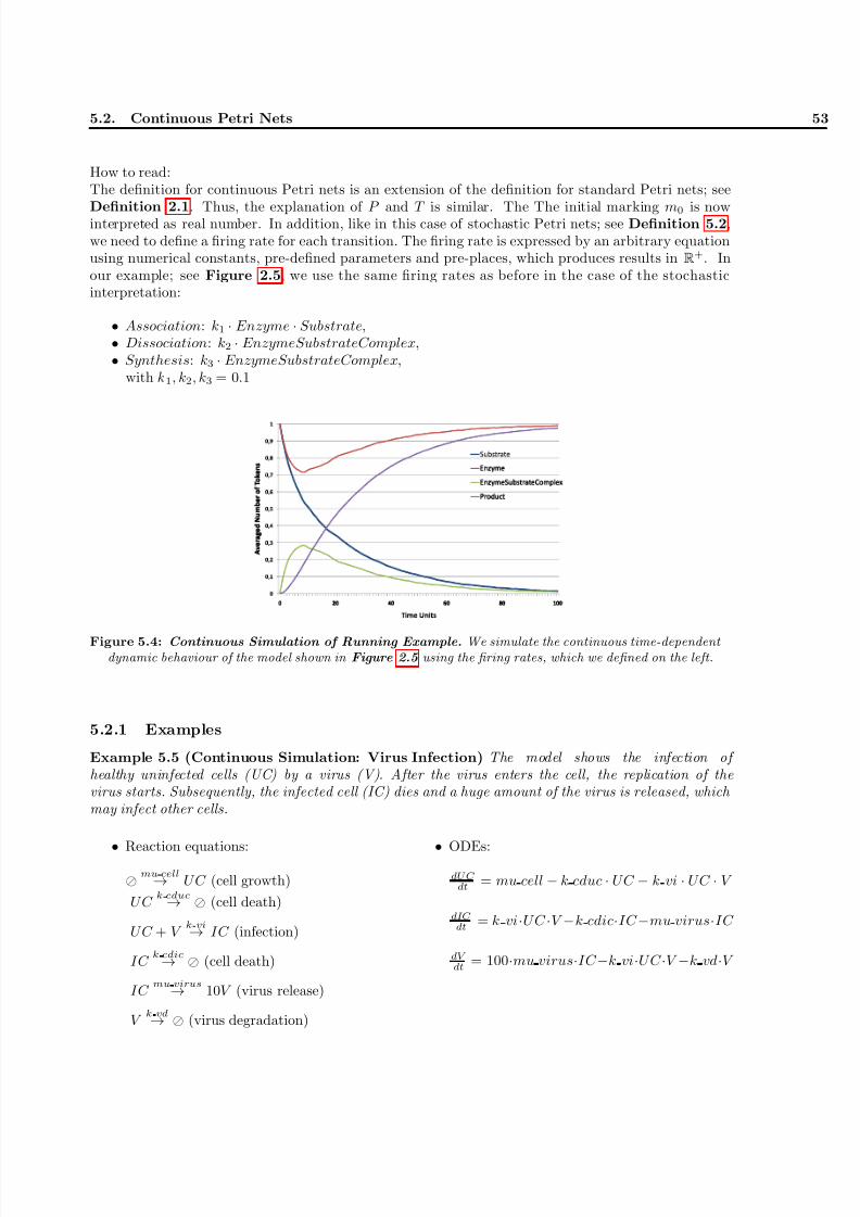
8/15/2019 Bla Et Ke Tutorial
http://slidepdf.com/reader/full/bla-et-ke-tutorial 61/108
5.2. Continuous Petri Nets 53
How to read:The definition for continuous Petri nets is an extension of the definition for standard Petri nets; see
Definition 2.1. Thus, the explanation of P and T is similar. The The initial marking m0 is nowinterpreted as real number. In addition, like in this case of stochastic Petri nets; see Definition 5.2,we need to define a firing rate for each transition. The firing rate is expressed by an arbitrary equationusing numerical constants, pre-defined parameters and pre-places, which produces results in R+. Inour example; see Figure 2.5, we use the same firing rates as before in the case of the stochasticinterpretation:
• Association: k1 · Enzyme · Substrate,• Dissociation: k2 · EnzymeSubstrateComplex,• Synthesis: k3 · EnzymeSubstrateComplex,
with k1, k2, k3 = 0.1
Figure 5.4: Continuous Simulation of Running Example. We simulate the continuous time-dependent dynamic behaviour of the model shown in Figure 2.5 using the firing rates, which we defined on the left.
5.2.1 Examples
Example 5.5 (Continuous Simulation: Virus Infection) The model shows the infection of healthy uninfected cells (UC) by a virus (V). After the virus enters the cell, the replication of the virus starts. Subsequently, the infected cell (IC) dies and a huge amount of the virus is released, which may infect other cells.
• Reaction equations:
mu cell
→ U C (cell growth)
U C k cduc
→ (cell death)
U C + V k vi
→ IC (infection)
IC k cdic
→ (cell death)
IC mu virus
→ 10V (virus release)
V k vd
→ (virus degradation)
• ODEs:dU C
dt = mu cell − k cduc · UC − k vi · UC · V
dIC dt
= k vi·U C ·V −k cdic·IC −mu virus·IC
dV dt
= 100·mu virus·IC −k vi·U C ·V −k vd·V

8/15/2019 Bla Et Ke Tutorial
http://slidepdf.com/reader/full/bla-et-ke-tutorial 62/108
54 Quantitative Petri Net Analysis
• Petri net: • Simulation:
Example 5.6 (Continuous Simulation: Lotka-Voltera Model) The Lotka-Voltera model (predator-prey model) is a famous model which describes the time-dependent oscillating behaviour of biological and ecological systems. The classic stability analysis of the model results in two fixed points. An unstable stable point, where the prey is eradicated, causing the predators to die of starvation.If predators are eradicated, the prey population grows infinitely. The second fixed point causes oscillation as shown here; the levels of the predator and the prey population cycle. A high number of predators leads to a low number of prey and vice versa.
• Reaction equations:
Prey k1→ 2Prey
Prey + Predator k2→ 2Predator
Predator k3→
• ODEs:
dPreydt
= k1 · Prey − k2 · Prey · Predator
dP redatordt
= k2·Prey ·Predator−k3·Predator
• Petri net: • Simulation:

8/15/2019 Bla Et Ke Tutorial
http://slidepdf.com/reader/full/bla-et-ke-tutorial 63/108
CHAPTER 6Model Checking for Petri Nets
In this chapter we introduce some basics about model checking for Petri nets and the use of temporallogics. In the next sections, we address to the following questions:
What is model checking in general?What are temporal logics?How to apply model checking with temporal logics to your system?
Be reminded that we just explain very basic facts about model checking and temporal logics. Werestrict ourself to an informal introduce of the here introduced concepts. Again we stick to the contentgiven in references [12] and [11].
6.1 Introduction to Model Checking
Model checking is an automatic, model-based, property-verification approach. It is used to proof thecorrectness of a model and ensure specific systems properties, e.g., in time. Originally, model checkinghas been designed to automatically verify software, concurrent and reactive systems (systems inter-acting with heir environment). Since biological systems contain concurrent mechanisms and interactwith environmental factors, model checking can also be used to verify models of biological system.In addition to general Petri net properties, model checking can be used to check special behaviouralproperties of the expected transient behaviour which reflect the intended functionality of the system.Properties are specified by mathematical equations using temporal logics; see Section 6.2. The truthof a specified property is determined by model checking.
The principle procedure of verifying a (biological) system via model checking is shown in Figure 6.1.The model checker gets an appropriate model of the system as input as well as system propertiesthat should be verified. System properties are formulated using linear temporal logics. The actualverification entails proving the truth of the defined property. In the case of correctness the output of the model checker is “true”, else the trace/path leading to the breach of the specified property maybedisplayed as a counter example.
6.2 Temporal Logics
To specify properties φ of a model temporal logics are employed. Temporal logic has found an importantapplication in formal verification, where it is used to state certain requirements of a system in a time
line. Beside the classical propositional logic, temporal logics allow to specify temporal relations by
55
8/15/2019 Bla Et Ke Tutorial
http://slidepdf.com/reader/full/bla-et-ke-tutorial 64/108
56 Model Checking for Petri Nets
Figure 6.1: Verification via Model Checking. Based on a (biological) system a model and properties of the system are derived. Properties that should be verified are formulated using temporal logics. Both, the specified properties and the model serve as input for the model checker. The model checker execute the verification step and proves the truth of the defined property. If the property is satisfied by the model, the output is “true”, else “false” and a counter example.
using additional operators (path quantifiers, temporal operators). Thereby, it is possible to describe,e.g., situation, where a certain state will be reached at the next time point, at some point, after anothercertain state or never. In a temporal logic you can express statements like “A certain signal moleculeis always synthesized”, “A certain signal molecule will eventually be synthesized”, or “A certain signalmolecule will be synthesized until the input signal is withdrawn”. Consider the statement: “A moleculeis produced”. Though its meaning is constant in time, the truth value of the statement can varyin time. Sometimes the statement is true, ans sometimes it is false, but it is never true and falsesimultaneously. In temporal logics, specified properties can have a truth value which can vary in time,where atemporal logic can not.Temporal logics always have the ability to reason about a time line. Temporal logics are distinguishedinto two classes: linear-time logics and branching-time logics; see Figure 6.2. Linear time logicsthink of time as a set of paths ; where a path is a sequence of time instances. Branching time logicsrepresent time as a tree. The tree is rooted at the present moment and branches out in the future.Thus, branching-time logics can reason about multiple time lines. This presupposes an environmentthat may act unpredictably. To continue the example above for branching-time logics, you can state“There is a possibility that a certain signal molecule will never be produced”.

8/15/2019 Bla Et Ke Tutorial
http://slidepdf.com/reader/full/bla-et-ke-tutorial 65/108
6.2. Temporal Logics 57
• Linear-time logics
– Set of paths
– A path is a sequence of states
– Every sate has an unique successor
– Infinite sequences
– Linear Time Temporal Logic (LTL),Probabilistic Linear Time TemporalLogic (PLTL)
• Branching-time logics
– Tree
– A tree consists of a root and severalbranches in the future
– Every sate has several successor
– Infinite tree
– Computation Tree Logic (CTL),Branching-time Continuous StochasticLogic (CSL)
Figure 6.2: Linear-time and Branching-time Logics. Temporal logics are used to specify properties of a Model. They can be categorized into linear-time logics (left) and branching-time logics (right) with distinct properties.
In the case of Petri nets, the path/traces needed for linear-time logics can be gained from theentire state space (reachability graph) of the model or from simulation. The computation tree need forbranching-time logics can only be constructed from the entire state space (reachability graph) of themodel. Indeed, model checking requires boundedness.Next, we will explain the most important temporal logics used for Petri nets: Computation TreeLogic (CTL) and Branching-time Continuous Stochastic Logic (CSL) represent branching-time logics.Linear Time Logic (LTL) and Probabilistic Linear Time Logic (PLTL) represent linear-time logics.Furthermore model checking can be divided into analytical model checking (CTL, CSL, LTL); seeSection 6.3, and simulative model checking (PLTL/LTLc); see Section 6.4. Model checking for Petrinets with the here introduced temporal logics can been done with Snoopy [19], Charlie [8] and/or Marcie [16]; see Table 6.1.
Table 6.1: Model Checking Tools and Temporal Logics
Snoopy [19] Charlie [8] Marcie [16]CTL + +CSL +LTL +PLTL +
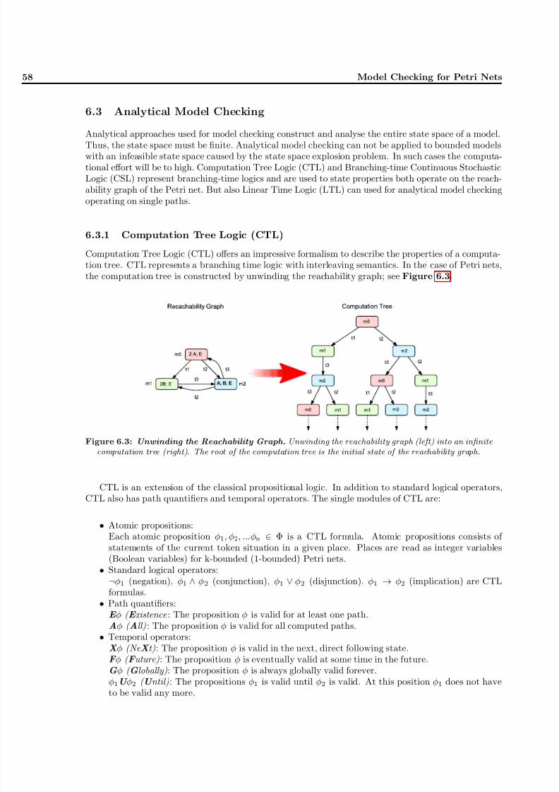
8/15/2019 Bla Et Ke Tutorial
http://slidepdf.com/reader/full/bla-et-ke-tutorial 66/108
58 Model Checking for Petri Nets
6.3 Analytical Model Checking
Analytical approaches used for model checking construct and analyse the entire state space of a model.Thus, the state space must be finite. Analytical model checking can not be applied to bounded modelswith an infeasible state space caused by the state space explosion problem. In such cases the computa-tional effort will be to high. Computation Tree Logic (CTL) and Branching-time Continuous StochasticLogic (CSL) represent branching-time logics and are used to state properties both operate on the reach-ability graph of the Petri net. But also Linear Time Logic (LTL) can used for analytical model checkingoperating on single paths.
6.3.1 Computation Tree Logic (CTL)
Computation Tree Logic (CTL) offers an impressive formalism to describe the properties of a computa-tion tree. CTL represents a branching time logic with interleaving semantics. In the case of Petri nets,
the computation tree is constructed by unwinding the reachability graph; see Figure 6.3.
Figure 6.3: Unwinding the Reachability Graph. Unwinding the reachability graph (left) into an infinite computation tree (right). The root of the computation tree is the initial state of the reachability graph.
CTL is an extension of the classical propositional logic. In addition to standard logical operators,CTL also has path quantifiers and temporal operators. The single modules of CTL are:
• Atomic propositions:Each atomic proposition φ1, φ2, ...φn ∈ Φ is a CTL formula. Atomic propositions consists of statements of the current token situation in a given place. Places are read as integer variables(Boolean variables) for k-bounded (1-bounded) Petri nets.
• Standard logical operators:¬φ1 (negation), φ1 ∧ φ2 (conjunction), φ1 ∨ φ2 (disjunction), φ1 → φ2 (implication) are CTLformulas.
• Path quantifiers:E φ ( E xistence : The proposition φ is valid for at least one path.Aφ ( All) : The proposition φ is valid for all computed paths.
• Temporal operators:X φ (Ne X t): The proposition φ is valid in the next, direct following state.F φ ( F uture): The proposition φ is eventually valid at some time in the future.G φ ( G lobally): The proposition φ is always globally valid forever.φ1U φ2 ( U ntil): The propositions φ1 is valid until φ2 is valid. At this position φ1 does not have
to be valid any more.
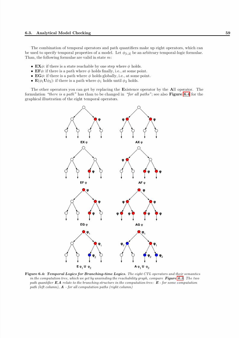
8/15/2019 Bla Et Ke Tutorial
http://slidepdf.com/reader/full/bla-et-ke-tutorial 67/108
6.3. Analytical Model Checking 59
The combination of temporal operators and path quantifiers make up eight operators, which canbe used to specify temporal properties of a model. Let φ[1,2] be an arbitrary temporal-logic formulae.
Than, the following formulae are valid in state m:
• EXφ: if there is a state reachable by one step where φ holds.• EFφ: if there is a path where φ holds finally, i.e., at some point.• EGφ: if there is a path where φ holds globally, i.e., at some point.• E(φ1Uφ2): if there is a path where φ1 holds until φ2 holds.
The other operators you can get by replacing the Existence operator by the All operator. Theformulation “there is a path” has than to be changed in “for all paths” ; see also Figure 6.4 for thegraphical illustration of the eight temporal operators.
Figure 6.4: Temporal Logics for Branching-time Logics. The eight CTL operators and their semantics in the computation tree, which we get by unwinding the reachability graph, compare Figure 6.3 . The twopath quantifier E ,A relate to the branching structure in the computation tree: E - for some computation path (left column), A - for all computation paths (right column)

8/15/2019 Bla Et Ke Tutorial
http://slidepdf.com/reader/full/bla-et-ke-tutorial 68/108
60 Model Checking for Petri Nets
Example 6.1 (CTL Model Checking: RKIP Pathway [11], see Example 4.1) Places are in-terpreted as Boolean variables in the following formulae, in order to simplify the notations.
• Property Q1: There is a state where ERK is phosphorylated and RKIP is not phosphorylated:
EF [(ERKpp ∨ Raf 1Star RKIP ERKpp) ∧
(RKIP ∨ Raf 1Star RKIP ∨ Raf 1Star RKIP ERKpp)]
Meaning: There is finally a state in one of the paths, where ERK is phosphorylated (ERKpp)or phosphorylated and bound to the Raf1Star-RKIP complex and RKIP, is in its initial state,in complex with Raf1Star or in complex with Raf1Star and ERK. This state corresponds to the marking m5 in the reachability graph. The shortest firing sequence is r6, r7.
• Property Q2: The phosphorylation of ERK (to ERKpp) is independent of the phosphorylation
of RKIP:
AG [(ERK ∧ ¬ (RKIPp ∨ RKIP p RP )) → E [¬ (RKIPp ∨ RKIP RP ) U ERKpp]]
Meaning: If we are in any state where ERK is phosphorylated and RKIP is not phosphorylated (RKIPp, RKIPp RP), then there is a path where RKIP can not become phosphorylated as long as ERK is not phosphorylated.
• Property Q3: A cyclic behaviour w.r.t. the presence/absence of RKIP is possible forever:
AG [(RKIP → EF (¬RKIP )) ∧ (¬RKIP → EF (RKIP ))]
Meaning: In any state where RKIP is marked exists a path to a state, where RKIP is not marked
any more, and vice versa.
Example 6.2 (CTL Model Checking: MAP Kinase Cascade [12], see Example 4.2) Places are interpreted as Boolean variables in the following formulae, in order to simplify the notations.
• Property Q1: There is just one possible pathway to fully activate ERK by passing through the states Rafp, MEKp, MEKpp and ERKp in order to reach ERKpp:
¬ [E (¬RAFpU MEKp) ∨ E (¬MEKpU MEKpp) ∨
E (¬MEKppU ERKp) ∨ E (¬ERKpU ERKpp)]
Meaning: it exists no path, where MEKp appears but RAFp has not been there; or where MEKppappears but MEKp has not been there; or where ERKp appears but MEKpp has not been there; or where ERKp appears but ERKpp has not been there.
• Property Q2: Dephosphorylation takes place independently. E.g., the duration of the phospho-rylated state is independent of the duration of the phosphorylated states of MEK and Raf:
(EF [RAF ∧ (ERKp ∨ ERKpp)] ∧ EF [RAFp ∧ (ERKp ∨ ERKpp)] ∧
EF [MEK ∧ (ERKP ∨ ERKPP )] ∧ EF [(MEKp ∨ MEKpp) ∧ (ERKP ∨ ERKPP )])
Meaning: There is a path that contains states, where Raf is not phosphorylated and ERK is phosphorylated (ERKp or ERKpp) and where Raf is phosphorylated (Rafp) and ERK is phospho-rylated, where MEK is not phosphorylated and ERK is phosphorylated and where MEK (MEKp
or MEKpp) is phosphorylated and ERK is phosphorylated.

8/15/2019 Bla Et Ke Tutorial
http://slidepdf.com/reader/full/bla-et-ke-tutorial 69/108
6.3. Analytical Model Checking 61
6.3.2 Branching-time Continuous Stochastic Logic (CSL)
In the case of stochastic Petri nets (see also Chapter 5.1), we can now apply Branching-time Contin-
uous Stochastic Logic (CSL). This allows to perform probabilistic analysis of the transient and steadystate behaviour. CSL uses the CTMC for the verification of properties, which is isomorph to the reach-ability graph. In addition to the state space, the firing rates are also involved in CSL to consider theprobability of a specified property. CSL replaces the path quantifiers (E, A) in CTL by the probabilityoperators Pp (transient analysis) and Sp (steady state analysis) whereby p specifies the proba-bility of the given formula (comparison operator can be replaced by <, ≤, =, =, >, ≥). The operatorP=? is used to return the probability (rather than compare probabilities).
• Pp [φ] - probability that paths fulfil φ is p• Sp [φ] - probability that φ holds in the steady state p
In CSL, we can now use the following abbreviation:
• trueUφ ⇒ Fφ• EFφ ⇒ P≥0 [Fφ]• AFφ ⇒ P≥1 [Fφ]
Example 6.3 (CSL Model Checking: RKIP Pathway [11], see Example 4.1) For the CSLmodel checking, we employ again a 7-level model. Places are now read as integer variables.
• Property S1a: There are reachable states where ERK is phosphorylated and RKIP is not phos-phorylated.
P >0 [F (ERKpp + Raf 1Star RKIP ERKpp ≥ 1∧
RKIP + Raf 1Star RKIP ERKpp + Raf 1Star RKIP = 7)]
• Property S2a: The phosphorylation of ERK (to ERKpp) is independent of the phosphorylated state of RKIP
P >? [G ((ERK = 7 ∧ RKIPp = 0 ∧ RKIPpRP = 0) →
P >0 [(RKIPp = 0 ∧ RKIP p RP = 0) U (ERKpp ≥ 1)])]
As this property always holds true, the returned probability is 1.
• Property S3a: A cyclic behaviour w.r.t. the presence/absence of RKIP is possible forever.
S >0 [RKIP = 0]
S >0 [RKIP ≥= 1]
Here the steady state operator is used to state the non-zero probabilities of RKIP being absent or present after long time, hence RKIP can cycle.
Example 6.4 (CSL Model Checking: MAP Kinase Cascade [12], see Example 4.2) For the CSL model checking, we employ again the model with 4 and 8 Levels. Than, we compute the probability of the suggested properties by varying the initial level L, e.g., 0-N. For the sake of efficiency, we restrict the U operator to 100 time steps. Places are now read as integer variables. (Note: expression in curly bracket {...} indicate the initial state.)
• Property S1a: What is the probability of Rafp increasing, when starting in a state where the amount of Rafp is for the first time at N:
P =?
(RafP = L) U <100
(RafP > L) {RafP = L}

8/15/2019 Bla Et Ke Tutorial
http://slidepdf.com/reader/full/bla-et-ke-tutorial 70/108
62 Model Checking for Petri Nets
Figure 6.5: Probabilities of the Accumulation of Rafp. The graphs show the probabilities of the accumulation of Rafp (A - Probability of property S1a, B - Probability of property S1b)as a function of the initial level. Here we compare the probabilities of two models with 4 and 8 total levels (reproduced from [ 12 ].
Figure 6.5 , A indicates that it is absolutely certain that the concentration of RAfp increases from an initial level 0. The Rafp concentration is not increasing from a level N. More precisely,the increase of Rafp is very likely for low levels. At intermediate levels the increase and decrease of Rafp is equal. The likelihood of an Rafp increase is very low (but not impossible) for high levels.Therefore, the total amount of Rafp will not accumulate in the first layer.
• Property S2a: What is the probability that, given the initial concentrations of Rafp, MEKpp,ERKpp being zero, the concentration of Rafp rises above some Level L while the concentration of MEKpp and ERKpp remain at zero, i.e., Rafp is the first to react?
P =?
((MEKpp = 0) ∧ (ERKpp = 0)) U <=100 (Rafp > L)
{(MEKpp = 0) ∧ (ERKpp = 0) ∧ (Rafp = 0)}]
Figure 6.5 , B points out, that it is very likely that Rafp rises, while MEKpp and ERKpp are zero for low levels of the upper half and even more likely for the bottom half if the levels. The decrease of the likelihood for higher level can be explained by property S1a. This property corresponds toproperties Q1 of Example 6.2 and C1 of Example 6.9 .
The analytical model checking approaches CTL and CSL have both high computational efforts.Analytical model checking constructs and analyses the entire state space, which might become infeasibledue to state explosion problems. Thus, analytical model checking becomes more and more impracticalwith increasing state space. Additionally, CTL and CSL can not handle unbounded models with infinite
state spaces. In order to avoid the enormous computational power required for large state spaces, time-dependent stochastic behaviour can be simulated by dedicated algorithms, and evaluated by simulativestochastic model checking or approximated by a deterministic continuous behaviour. Simulative modelchecking we be considered in the following sections.
6.3.3 Linear Time Logic (LTL)
As indicated before the Linear Temporal Logic (LTL) operates along paths. Paths are extracted fromthe reachability graph. In addition, paths could also be generated by simulating the time-dependent dy-namic behaviour of model if stochastic and continuous Petri nets are used. In that case, the probabilisticextension of LTL (PLTL) should be considered; see Section 6.4.1. LTL allows to make statementsabout (all) paths staring in a state. In contrast to CTL, LTL uses no path quantifiers; see Figure 6.6.
Thus, LTL implies the same modules as CTL despite of the path quantifiers; compare Section 6.3.1.
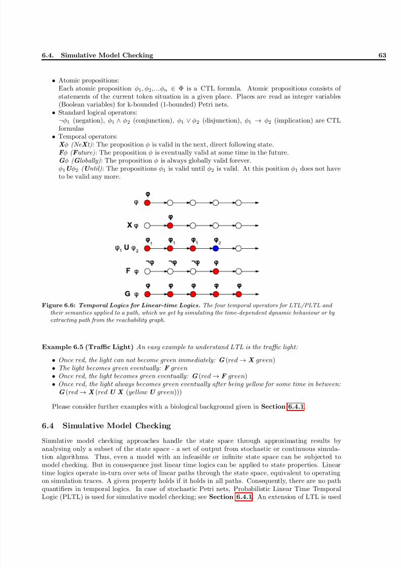
8/15/2019 Bla Et Ke Tutorial
http://slidepdf.com/reader/full/bla-et-ke-tutorial 71/108
6.4. Simulative Model Checking 63
• Atomic propositions:Each atomic proposition φ1, φ2,...φn ∈ Φ is a CTL formula. Atomic propositions consists of
statements of the current token situation in a given place. Places are read as integer variables(Boolean variables) for k-bounded (1-bounded) Petri nets.• Standard logical operators:
¬φ1 (negation), φ1 ∧ φ2 (conjunction), φ1 ∨ φ2 (disjunction), φ1 → φ2 (implication) are CTLformulas
• Temporal operators:X φ (Ne X t): The proposition φ is valid in the next, direct following state.F φ ( F uture): The proposition φ is eventually valid at some time in the future.G φ ( G lobally): The proposition φ is always globally valid forever.φ1U φ2 ( U ntil): The propositions φ1 is valid until φ2 is valid. At this position φ1 does not haveto be valid any more.
Figure 6.6: Temporal Logics for Linear-time Logics. The four temporal operators for LTL/PLTL and their semantics applied to a path, which we get by simulating the time-dependent dynamic behaviour or by extracting path from the reachability graph.
Example 6.5 (Traffic Light) An easy example to understand LTL is the traffic light:
• Once red, the light can not become green immediately: G (red → X green)• The light becomes green eventually: F green• Once red, the light becomes green eventually: G (red → F green)• Once red, the light always becomes green eventually after being yellow for some time in between:
G (red → X (red U X (yellow U green)))
Please consider further examples with a biological background given in Section 6.4.1.
6.4 Simulative Model Checking
Simulative model checking approaches handle the state space through approximating results byanalysing only a subset of the state space - a set of output from stochastic or continuous simula-tion algorithms. Thus, even a model with an infeasible or infinite state space can be subjected tomodel checking. But in consequence just linear time logics can be applied to state properties. Lineartime logics operate in-turn over sets of linear paths through the state space, equivalent to operatingon simulation traces. A given property holds if it holds in all paths. Consequently, there are no pathquantifiers in temporal logics. In case of stochastic Petri nets, Probabilistic Linear Time Temporal
Logic (PLTL) is used for simulative model checking; see Section 6.4.1. An extension of LTL is used

8/15/2019 Bla Et Ke Tutorial
http://slidepdf.com/reader/full/bla-et-ke-tutorial 72/108
64 Model Checking for Petri Nets
to specify properties of the model for simulative model checking. For continuous simulation LTLc, anmodification of LTL is employed Section 6.4.2.
6.4.1 Probabilistic Linear Time Logic (PLTL)
The Probabilistic Linear Time Logic (PLTL) extends the standard LTL to a stochastic setting. InPLTL we also use the probability operators Pp such as in CSL, and a filter construct, {φ}, definingthe initial state of the property. PLTL can be considered as a linear time counterpart to CSL. In PLTLembed probability operators are not allowed. PLTL can not be used to perform steady state analysis.The temporal operators in PLTL do not requires time bounds.PLTL operates along sets of linear paths (traces) of temporal behaviour, which are generated by stochas-tic simulation runs. Each generated trace is evaluated to a Boolean truth value, and the probabilityof a property holding true is computed by the fraction of true values in the set over the whole set.Thus model checking with PLTL incorporates two approximations. The truth value of a single trace isapproximated by operating over a finite sequence of states only, and the probability of the property is
approximated through sampling a finite number of traces (a subset of the model’s behaviour) only.With the help of PLTL, you can easily evaluate the time-dependent behaviour of a model generatedby stochastic simulation runs, as well as experimental time series data. Using PLTL allows to employa greater number of tokens than in the case of analytical model checking. The efficiency of PLTL ismuch higher. In general, for very high numbers of molecules, the stochastic behaviour tends to thedeterministic behaviour of the model.Simulative model checking has its advantage when the range of behaviours that the model checkeroperates over becomes computationally infeasible. The simulative approach allows to check a propertyin a feasible time through approximating the state space of the model.
Example 6.6 (PLTL Model Checking: RKIP Pathway [11], see Example 4.1) Places are read as integer variables. The properties are checked using 100 simulation traces from Gillespie’s
algorithm with a simulation time of 10, 000 s.
• Property S1s: There are reachable states where ERK is phosphorylated and RKIP is not phos-phorylated.
P >0 [F (ERKpp + Raf 1Star RKIP ERKpp ≥ 1∧
RKIP + Raf 1Star RKIP ERKpp + Raf 1Star RKIP = 7)]
• Property S2s: The phosphorylation of ERK (to ERKpp) is independent of the phosphorylated state of RKIP
P ≥1 [(RKIPp + RKIPp RP = 0) U (ERKpp ≥ 1)]
Remember, that embed probability operators are not allowed in PLTL. Thus, this property is much weaker than in the case of CSL. The property says, from the initial state of the system, ERK can phosphorylate without RKIP being phosphorylated. In fact, this is always true from the initial state.
• Property S3s: A cyclic behaviour w.r.t. the presence/absence of RKIP is possible forever.
P >0 [F (RKIP ≥ 1) {time ≥ 5000 ∧ RKIP = 0}]
P >0 [F (RKIP ≥ 0) {time ≥ 5000 ∧ RKIP ≥ 1}]
Direct steady state analysis is not possible in PLTL. But steady state analysis can be approximated by very long simulation runs. Than, the property is checked at/near the end of the simulation.Here, the property of RKIP being absent and present. Here, the property of RKIP being absent
and present in turns holds for long simulation runs.

8/15/2019 Bla Et Ke Tutorial
http://slidepdf.com/reader/full/bla-et-ke-tutorial 73/108
6.4. Simulative Model Checking 65
Figure 6.7: Simulative Model Checking of Property S1s. Simulative model checking of property S1s at a varying number of molecules; 4, 40, 400, 4000. This shows a progression towards the deterministic
behaviour as the number of molecules increases (reproduced from [ 12] .
Example 6.7 (PLTL Model Checking: MAP Kinase Cascade [12], see Example 4.2)Places are read as integer variables. The properties are checked using 100 simulation traces from Gillespie’s algorithm with a simulation time of 300 s.
• Property S1s: What is the probability of the concentration of Rafp increasing, when starting in a state where the level is for the first time at L:
P =? [(RafP = L) U (RafP > L) {RafP = L}]
Figure 6.7 illustrates the probability of Rafp increasing for the stochastic and deterministic be-
haviour varying the amount of molecules from 4 up to 4000 molecules. From the deterministic

8/15/2019 Bla Et Ke Tutorial
http://slidepdf.com/reader/full/bla-et-ke-tutorial 74/108
66 Model Checking for Petri Nets
Figure 6.8: Simulative Model Checking of Property S2s. Simulative model checking of property S2s at a varying number of molecules; 4, 40, 400, 4000. This shows a progression towards the deterministic
behaviour as the number of molecules increases (reproduced from [ 12] .
behaviour it can be observed, that the Rafp will always increase until it reaches the maximum num-ber, which corresponds to a concentration of around 0.1182 mMol. With increasing molecules, the maximum possible number of molecules in the stochastic behaviour of Rafp tends towards the de-terministic behaviour. In more detail, the stochastic behaviour tends to a probability of 0.5. in its possible concentration range, due to the steady increase and decrease.
• Property S2s: What is the probability that, given the initial concentrations of Rafp, MEKpp,
ERKpp being zero, the concentration of Rafp rises abvoe some Level L while the concentration of

8/15/2019 Bla Et Ke Tutorial
http://slidepdf.com/reader/full/bla-et-ke-tutorial 75/108
6.4. Simulative Model Checking 67
MEKpp and ERKpp remain at zero, i.e., Rafp is the first to react?
P =? [((MEKpp = 0) ∧ (ERKpp = 0)) U (Rafp > L)
{(MEKpp = 0) ∧ (ERKpp = 0) ∧ (Rafp = 0)}]
Figure 6.8 shows, that the stochastic behaviour drifts against the deterministic behaviour. In the deterministic scenario, the probability for ERKpp, MEKpp and Rafp being 0 is just given at the initial, else the probability is 1. The stochastic behaviour becomes less curved and more step-like shaped with an increasing amount of molecules and thereby tends towards the vertical line in the deterministic behaviour.
6.4.2 Continuous (Probablistic) Linear Time Logic (LTLc/PLTLc)
In the case of continuous Petri nets, the discrete number of tokens is replaced by continuous value.Hence, the deterministic behaviour can not describe the behaviour of individual levels of molecules but
their concentration. Repeated deterministic simulation will always yield into the same time-dependentbehaviour. The state space of such models is continuous and linear. The natural choice to analysiscontinuous linear behaviour are natural linear time-dependent logics like LTL and PLTL. Here, LTLand PLTL are used in a deterministic setting and interpreted over the continuous simulation trace of ODEs. The deterministic model has only on (averaged) behaviour. Thus, the resulting probability forproperties formalized in PLTL is 1 or 0.
Example 6.8 (LTLc Model Checking: RKIP Pathway [11], see Example 4.1) Places are in-terpreted as real number variables. We used a simulation time of 10, 000 s to evaluate the deterministic behaviour. We use parameter significant and noise to compare the concentration of spezies with cer-tain thresholds. In this example, we applied PLTL to formalize the properties. All properties can be transferred into the LTL setting as well.
• Property C1: There are reachable states where ERK is phosphorylated and RKIP is not phos-phorylated.
P ≥1 [F (ERKpp + Raf 1Star RKIP ERKpp > noise∧
RKIP + Raf 1Star RKIP ERKpp + Raf 1Star RKIP ≥ significant)]
• Property C2: The phosphorylation of ERK (to ERKpp) is independent of the phosphorylated state of RKIP
P ≥1 [(RKIPp + RKIPp RP ≤ noise) U
(ERKpp + Raf 1Star RKIP ERKpp > noise)]
Remember, that embed probability operators are not allowed in PLTL. Thus, this property is much weaker than in the case of CSL. The property says, from the initial state of the system, ERK can phosphorylate without RKIP being phosphorylated. In fact, this is always true from the initial state.
• Property C3: A cyclic behaviour w.r.t. the presence/absence of RKIP is possible forever.
P ≤0 [F (RKIP ≥ 1) {time ≥ 5000 ∧ RKIP ≤ noise}]
P ≤0 [F (RKIP ≤ noise) {time ≥ 5000 ∧ RKIP < noise}]
Direct steady state analysis is not possible in PLTL. But steady state analysis can be approximated by very long simulation runs. Than, the property is checked at/near the end of the simulation.Here, the property of RKIP being absent and present. Here, the property of RKIP being absent
and present in turns holds for long simulation runs.

8/15/2019 Bla Et Ke Tutorial
http://slidepdf.com/reader/full/bla-et-ke-tutorial 76/108
68 Model Checking for Petri Nets
Example 6.9 (LTLc Model Checking: MAP Kinase Cascade [12], see Example 4.2) Places are interpreted as real number variables. We used a simulation time of 400 s to evaluate the determin-
istic behaviour. We use parameter significantspecies and noisespecies to compare the concentration of a species (Rafp, MEKpp, ERKpp) with certain their thresholds. In this example, we applied LTL to formalize the properties. All properties can be transferred into the PLTL setting as well. Note, that properties C1, C2 and C3 correspond to the qualitative properties Q1; see Example 6.2 ., and that S2 of Example 6.7 is the stochastic counterpart of C1.
• Property C1: The concentration of Rafp rises to a significant level, while the concentration of MEKpp and ERKpp remain close zero, i.e., Rafp is really the first species to ract:
((MEKpp < noiseMEKpp) ∧ (ERKpp < noiseERK )) U (Rafp > significantRafp)
• Property C2: If the concentration of Rafp is at a significant concentration level and that of ERKpp is close to zero, them both species remain in these state until the concentration of MEKpp
becomes significant, i.e., MEKpp is the second species to react:
((Rafp > significantRafp) ∧ (ERKpp < noiseERK )) ⇒
((Rafp > significantRafp) ∧ (ERKpp < noiseERK )) U (MEKpp > significantMEKpp)
• Property C3: If the concentration of Rafp and MEKpp are significant, they remain so, until the concentration of ERKpp becomes significant, i.e., ERKpp is the third species to react:
((Rafp > significantRafp) ∧ (MEKpp > significantMEKpp)) ⇒
((Rafp > significantRafp) ∧ (MEKpp > significantMEKpp)) U (ERKpp > significantERKpp)

8/15/2019 Bla Et Ke Tutorial
http://slidepdf.com/reader/full/bla-et-ke-tutorial 77/108
CHAPTER 7Petri Net Editor: Snoopy
In this chapter, we introduce the Petri net editor Snoopy [19]. The following information about Snoopy can also be looked up in detail in references [19, 14]. Snoopy is a tool to design and animate hierarchicalgraphs, among others Petri nets. Thus, Snoopy allows constructing of Petri nets, as well as to animateand simulate the resulting token-flow. The tool has been developed - and is still under development- at the University of Technology in Cottbus [3], Dep. of Computer Science, “Data Structures andSoftware Dependability” [1]. The tool is in use for the verification of technical systems, especiallysoftware-based systems, as well as for the validation of natural systems, i.e., biochemical networks asmetabolic, signal transduction, gene regulatory networks. Several Petri net classes are comprised in theunifying framework offered by Snoopy , like qualitative, stochastic, continuous and Hybrid Petri nets and
in addition the coloured counterparts. Snoopy facilitates the consideration of the qualitative networkstructure of a model under specific kinetic aspects of the specialized Petri net class. The frameworkof Snoopy allows investigating Petri net models in various complementary ways. Therefore, Petri netmodels can be converted into each other. Different Petri net classes can be used simultaneously inSnoopy .
The three outstanding main characteristics of Snoopy are:
1. it is extensible ; it’s generic design facilitates the implementation of new Petri net classes2. it is adaptive ; several models can be used simultaneously, the graphical user interface adapts
dynamically to the network class in the active window3. it is platform independent ; it is executable on all popular operating systems (linux, mac, windows)
Two specialized types of nodes support the design, systematic construction and neat arrangementof large Petri nets. Logical nodes act as connector or multiple used places or transitions sharing thesame factor or function. Macro nodes allow to hierarchically design a Petri net.All elements in each Petri net class can be individually edited and coloured. Computed node sets canbe visualized on the network structure. The network layout can be changed manually or automatically.Syntactical errors in the network structure of a Petri net is prevented by the implementation of thegraphical editor.The tool design of Snoopy and its features facilitate the intuitive construction of Petri nets and theanimation/simulation of the time-dependent dynamic behaviour. Snoopy is still under development andtries to cope with the needs of biological models. The constructed Petri net models can be exportedand analysed in Charlie .The next chapters are concentrated on the stochastic Petri net class. All other Petri net classes are
similarly built.
69

8/15/2019 Bla Et Ke Tutorial
http://slidepdf.com/reader/full/bla-et-ke-tutorial 78/108
70 Petri Net Editor: Snoopy
7.1 Editor Mode
In this section, we explain the graphical user interface of the editing mode in Snoopy based on thestochastic Petri net class.First, to open a new document, you have to start Snoopy and go to File/New or press the new button inthe tool bar . A template dialogue opens, where you can now select the document template; see Figure7.1.
Figure 7.1: Select Template.A new template of the chosen Petri net class can be opened in this dialogue.
Figure 7.2: Graphical Editor User Interface in Snoopy. The window is divided into four functional units: Menu bar (contains several functions), Tool bar (contains some short cuts), Graph elements (lists all available elements), Hierarchy browser (lists all levels) and Editor pane (canvas)

8/15/2019 Bla Et Ke Tutorial
http://slidepdf.com/reader/full/bla-et-ke-tutorial 79/108
7.2. Elements of the Stochastic Petri Net Class 71
Figure 7.2 shows the graphical editor user interface in Snoopy of the stochastic Petri net class.The drop down menus in the Menu bar offer the following commands:
• File : New/Open/Close Window/Save/Save as, Print, Export/Import, Preferences (change thedefault visualisation) and Exit
• Edit : Undo/Redo, Select All/Copy/Copy in new net/Paste/Cut, Clear/Clear all, Hide/Unhide,Edit selected elements/Transform Shapes, Layout (automatic layout function), Sort Nodes (by IDor name), Check Net (duplicate nodes, syntax, consistency) and Convert to
• View : Zoom 100%/Zoom In/Zoom Out, Net Information (numer of each element used in themodel), Toogle Graphelements/Hierachy browser/Filebar/Log window, Show Attributes (choosefor each elements which attributes to be shown in the model), Start Anim-Mode/Simulation-Mode/Steering-Mode
• Elements (list of all available elements): Select/ Place/Transition/ Coarse Place/Coarse Tran-sition/ Immediate Transition/Deterministic Transition/Scheduled Transition/Parameter/CoarseParameter/LookupTable, Edge/Read Edge/Inhibitor Edge/Reset Edge/Equal Edge/Modifier
Edge and Comment• Hierarchy (edit and browse hierarchy): Coarse (chosen elements are encapsulate in a macro
node)/Flatten (chosen macro nodes are decapsulate) and Go Up in Hierarchy/Go To First Childin Hierarchy/Go To Next Sibling in Hierarchy/o To Previous Sibling in Hierarchy
• Search : Search nodes (by ID or name)• Extra : Load node sets (visualise, e.g., T-, P-invariants, siphons and traps), Interaction and General
Information (title, author, description, literature)• Window (arrange all opened windows): Cascade/Tile Horizontally/Tile vertically, Arrange
Icons/Next/Previous and Open Files• Help: Help, About (current version), check update
The tool bar contains four short cuts to:
• Open a new document;• Load a document;• Save a document;• Select an element.
The panel for the Graph elements displays all elements available in the current net class. To useone of them make a left-click on one of the elements. To edit or select all elements of the same class,use a right click on the respective element in the Graph elements panel.
The Hierarchy Browser lists all levels. A left-click the chosen hierarchical level opens the subnet ina new window.
The Editor pane is the canvas, on which to draw the network. Activate the element you want touse in Graph elements panel to use it on the canvas. A left-click on the Editor pane places the selectedelement on the canvas. To draw an arc between two nodes click left onto one node, hold the left-click
and drag the line to the other node, now drop the left-click. To add edges to an arc push the CRTL keyand click left on the arc. You can now drag the edge with another left-click. For a better orientationon the canvas, it is possible to use a grid which can be activated under File/Preferences in the canvas tab. You can also choose between to two edge styles in the Preference dialogue in the elements tab,choose among line or spline .
7.2 Elements of the Stochastic Petri Net Class
Next, we provide an overview of all elements available in the stochastic Petri net class in Snoopy , theirvisualisation and attributes; see Table 7.1. In the following subsections, all elements are explained inmore detail.

8/15/2019 Bla Et Ke Tutorial
http://slidepdf.com/reader/full/bla-et-ke-tutorial 80/108
72 Petri Net Editor: Snoopy
Table 7.1: bersicht zu den Petri-Netz-Elementen und ihren Attributesn
Types of Nodes Elements Graphic Attributes
Standard Place ID, name, marking, comment, logic, graphic
Standard Transition ID, name, function, comment, logic, graphic
Coarse Place name, comment, graphic
Coarse Transition name, comment, graphic
Immediate Transition ID, name, weight function, comment, logic, graphic
Deterministic Transition ID, name, delay, comment, logic, graphic
Scheduled Transition ID, name, begin/repetition/end, comment, logic,graphic
Edge Elements Graphic Attributes
Standrad Edge ID, arc weight, comment, graphicRead Edge ID, arc weight, comment, graphicInhibitor Edge ID, arc weight, comment, graphicReset Edge ID, comment, graphicEqual Edge ID, arc weight, comment, graphic
Modifier Edge ID, comment, graphic
Additional elements for modeling Elements Graphic Attributes
Lookup Table ID, name, (x, f(x))- values, graphic
Parameter ID, name, parameter value, comment, graphic
Coarse Parameter name, comment, graphic
Comment comment, graphic
You can edit the attributes of each element. A double click on an element opens a property dialogue with different tabs where you can now modify the attributes of the chosen element. Here, we show asexample the place editing dialogue in Figure 7.3. Advantageously, you can edit several elements at thesame time by selecting all elements you like to edit.
7.2.1 Places
Snoopy offers two types of places, the standard place and the coarse place . Coarse places correspond tomacro places and facilitate the hierarchical arrangement of Petri nets by opening a new layer to model
a place in more detail; see Section 2.3.1.

8/15/2019 Bla Et Ke Tutorial
http://slidepdf.com/reader/full/bla-et-ke-tutorial 81/108
7.2. Elements of the Stochastic Petri Net Class 73
Figure 7.3: Place Dialogue. In the first tab ”General”, the name of the place can be changed, comments can be provided and the place can be declared as logic. In the tab ”Marking” (not available for coarse places), the number of tokens of the corresponding place can be specified (default is zero). The ”Graphic”tab allows you to change the visualisation of the place.
7.2.2 Transitions
Several types of transitions are available in Snoopy . Among them are standard transitions and coarse transitions . Coarse transitions correspond to macro transitions and facilitate the hierarchical arrange-ment of Petri nets by opening a new layer to model a transition in more detail; see Section 2.3.1. There
are three more specific transitions available: deterministic transitions , immediate transitions and sched-uled transitions . Those specific transitions are very useful to model timed input signals correspondingto the wet-lab experiment.
Figure 7.4 explains the differences between the different types of transition. The rate function of the standard transitions and the weight function of the immediate transition can be defined byvarious mathematical equations. Snoopy offers a function/weight assistant to define such mathematicalexpressions; see Figure 7.5. The function/weight assistant indicates which elements are allowed to beused in the equation; see Figure 7.5. In general, you can use pre-places of a transition and parameters to define the respective rate/weight function . Places that are not a pre-place of a transition can not beused in rate/weight functions. If you want to use such places in the firing rate, they must be connectedwith the respective transition via a modifier edge ; see Section 7.2.3. Places connected via a modifier arc with a transition do affect the kinetic, but not the ability of the transition to be enabled. The function/weight assistant also offers several pre-defined mathematical functions that can be used to
define individual equations; see Table 7.3.
Table 7.2: Classification and Meaning of specific transitions.
Transition Type Informal Definition Meaning
Immediate Transition Immediate Transition Immediate transitions fire as soon as they areenabled. The waiting time is equal to zero.
Standard Transition Timed Transition A waiting time is computed as soon as thetransition is enabled. The transition fires if the timer elapsed zero and the transitions isstill enabled.

8/15/2019 Bla Et Ke Tutorial
http://slidepdf.com/reader/full/bla-et-ke-tutorial 82/108
74 Petri Net Editor: Snoopy
Deterministic Transition Fixed timed transi-tions with periodic
firing trails
Deterministic transitions fire as soon as thefixed time interval elapses during the entire
simulation run time. The respective determin-istic transitions must be enabled at the end of each repeated interval.
Scheduled Transition Fixed timed transi-tions with periodicfiring trails betweentwo time points
Scheduled transitions fire as soon as the fixedtime interval elapsed during the given time-points. The respective deterministic transi-tions must be enabled at the end of each re-peated interval.
Figure 7.4: Comparison of the Standard Transitions and Specific Transitions. For each transition,we show here its functionality by simulating their time-dependent dynamic behaviour. See also Table 7.2
for further explanations.

8/15/2019 Bla Et Ke Tutorial
http://slidepdf.com/reader/full/bla-et-ke-tutorial 83/108
7.2. Elements of the Stochastic Petri Net Class 75
Table 7.3: Pre-defined mathematical Functions.
Name Meaning of the FunctionBioMassAction(.) Stochastic law of mass action. Tokens are interpretated as singlemolecules.
BioLevelInterpretation(.) Stochastic law of mass action. Tokens are interpretated as concentration.ImmediateFiring(.) Refers to immediate transitions.TimedFiring(.) Refers to deterministic transitions.FixedTimedFiring Single(.) Refers to deterministic transitions that only fires once after a given time-
point.FixedTimedFiring(., ., .) Refers to scheduled transitions.abs(.) Absolute valueacos(.) Arc cosine functionasin(.) Arc sine function
atan(.) Arc tangent functionceil(.) Rounding upcos(.) Cosine functionexp(.) exponential functionsin(.) Sine functionsqrt(.) Square roottan(.) Tangent functionfloor(.) Round off log(.) Natural logarithm with constant e as baselog10(.) Common logarithm with constant 10 as basepow(.) Exponent
Figure 7.5: Rate/Wight Assistant. The rate/weight assistant helps to define mathematical functions. All allowed elements (places, parameters) that can be used to define the rate/weight function of a transition are displayed. The assistant also offers several pre-defined mathematical functions that can be used to define rate/weight function. In addition, the assistant proofs whether or not the semantic of the equation is correct.
7.2.3 Edges
In addition to the standard edge , Snoopy offers also several specific edge types: read edge , inhibitor edge ,
reset edge , equal edge and modifier edges . Those specific edge types can be very useful to model certain

8/15/2019 Bla Et Ke Tutorial
http://slidepdf.com/reader/full/bla-et-ke-tutorial 84/108
76 Petri Net Editor: Snoopy
scenarios, e.g., timed inputs, different stimulation patterns. The function of those specific edge types isexplained in Table 7.4.
Table 7.4: Edge types and their meanings.
Edge Illustration Meaning
Standard Edge The transition is enabled and may fire if both pre-places Aand B are sufficiently marked by tokens. After firing of thetransition, tokens are removed from the pre-places A and B;new tokens are produced on place C.
Read Edge The transition is enabled and may fire if both pre-places Aand B are sufficiently marked by tokens. After firing of thetransition, tokens are removed from the pre-place B but not
from pre-place A; new tokens are produced on place C. Thefiring of the transition does not change the amount of tokenson pre-place A.
Inhibitor Edge The transition is enabled and may fire if pre-place B is suffi-ciently marked by tokens. The amount of tokens on pre-placeA must be smaller than the given arc weight. After firing of thetransition, tokens are removed from the pre-place B but notfrom pre-place A; new tokens are produced on place C. Thefiring of the transition does not change the amount of tokenson pre-place A.
Reset Edge The transition is enabled and may fire if pre-place B is suffi-ciently marked by tokens. The amount of tokens on pre-placeA has no effect on the ability to enable the transition and af-fects only the kinetics. After firing of the transition, tokens areremoved from the pre-place B according the arc weight and alltokens on pre-places A are deleted; new tokens are producedon place C.
Equal Edge The transition is enabled and may fire if number of tokenson pre-place A is equal to the correpsonding arc weight andplace B is sufficiently marked. After firing of the transition,tokens are removed from the pre-place B but not from pre-place A; new tokens are produced on place C. The firing of thetransition does not change the amount of tokens on pre-placeA.
Modifier Edg e The transition is enabled and may fire if pre-place B is suffi-ciently marked with tokens. The amount of tokens on pre-placeA has no effect on the ability to enable the transition and af-fects only the kinetics. After firing of the transition, tokens areremoved from the pre-place B but not from pre-place A; newtokens are produced on place C. The firing of the transitiondoes not change the amount of tokens on pre-place A.

8/15/2019 Bla Et Ke Tutorial
http://slidepdf.com/reader/full/bla-et-ke-tutorial 85/108
7.3. Configuration Sets 77
7.2.4 Parameters
The element parameter can be used to define individual parameters. Parameters can be used to define
rate/weight functions but not to define the number of tokens on a certain place. Coarse parameters are a third group of macro elements, which allow encapsulating parameters . Thereby, high numbers of parameters are not visible on the top-level or can also be categorized by the use of coarse parameters .
7.3 Configuration Sets
Snoopy supports the deposition of configuration sets for each type of node (e.g. standard places , standard transitions ) and parameter s; see Figure 7.6. Configuration sets offer a fast and convenient way toflexibly switch between, e.g., different initial markings, firing rates and parameter values at once.The editing, adding and deletion of configuration sets is organized an overview dialogue . The buttonto display the overview dialogue can be found in editor dialogue of each type of node or parameter . ForThe standard configuration set for these elements can not be deleted or renamed. All configuration sets
can be exported using file/export/export to CSV . The chosen configuration sets will be displayed on thePetri net itself and used for animation and simulation.
Figure 7.6: Configuration Set. For each type of node and parameter exists an overview, where all elements are displayed and their values (marking, rate/weight function, parameter value). In the overview dialogue it is possible to edit single entries, to add new sets, rename set and delete sets.
7.4 Animation Mode
The animation mode in Snoopy allows you to observe the token-flow; see Figure 7.7. To start theanimation mode go to View/Start Anim-Mode or simply press F5 . A new window opens, where you cannow steer the animation. The animation mode is very useful to get a first expression of the causality of a model and how it works. Playing with the token-flow in the animation mode may help to understandthe modelled mechanism.You can animate the token-flow manually by clicking on the transition. If you want to fire a transitionthat is not enabled, you get the notification “This transition is not enabled”. You can quickly add tokensby clicking-left on a place and withdraw tokens by clicking-right on a place. You can also animate thetoken-flow by using the radio buttons on the animation steering panel . The animation can be controlledvia the radio buttons step-wise forward and backward or sequentially as long as one transition can beenabled, otherwise you get the notification “Dead State: There are no more enabled transitions.”. In
the animation steering panel you find also information about the transition with the shortest waiting

8/15/2019 Bla Et Ke Tutorial
http://slidepdf.com/reader/full/bla-et-ke-tutorial 86/108
78 Petri Net Editor: Snoopy
time which fires next. You can also change further animation properties under options , like refreshment ,duration and stepping .
In the animation mode , you have also access to the configuration sets . You can choose, which configu-ration sets , you want to use for the animation of the token-flow. The “Stochastic Simulation” buttonat the bottom of the dialogue starts the stochastic simulation mode .
Figure 7.7: Animation Mode. The token-flow can be animated by clicking on a transition or via the control keys in the animation steering panel.
7.5 Simulation Mode
To perform stochastic simulations with the current model in the active window, you can start thestochastic simulation mode : View/Start Simulation , simply press F6 or use the stochastic simulation button the animation control panel .The stochastic simulation mode allows you to simulate the time-dependent dynamic behaviour of the
model indicated by the token-flow or the firing frequency of the transitions. The token-flow indicateshow the concentration levels or the discrete number of the components change over time. The firingfrequency shows how often reactions are performed during the simulation time. Thus, you will get animpression of the time-dependent changes in your model, which might help to understand the wet-labsystem. You can perform several simulation studies with your model by manipulating the structureand/or perturbing the initial state (test various stimuli, mutations, knock-outs/downs etc.) and kinetics.All results can be manually or automatically exported in the standard *.csv-format and thus, can beprocessed and analysed in other mathematical programs.
The graphical interface of the stochastic simulation mode can be divided in three functional units;see Figure 7.8:
• Simulation Control : The simulation control allows choosing the main settings and properties for
the simulation. It can be further divided in 4 panels:

8/15/2019 Bla Et Ke Tutorial
http://slidepdf.com/reader/full/bla-et-ke-tutorial 87/108
7.5. Simulation Mode 79
Figure 7.8: Simulation Mode. The graphical simulation interface is tripartite, consisting of a panel for the simulation control to change the setting and simulation properties (red), display of simulation results as table or plot (green), viewer/node choice.
– Configuration Sets : Modify configuration sets by editing single entries or adding new setsand choosing the configuration sets that should be used for the simulation run.
– Simulation Properties : Set interval start (time-point from which simulation results should bedisplayed), interval end (time-point where the simulation ends) and output step count (num-ber of time-points that should be displayed in the given interval), choose simulator (Gillespieor FAU) and change other properties, e.g., simulation run count (number of simulation runsthat should be performed to average the simulation results).
– Export Properties : Different automatic export settings are available to the *.csv-format.– Start Simulation : Start simulation with the chosen settings and properties. The bar indicates
the progress of the simulation and the required time is given below.
• Viewer/Node Choice : Choose which and how you want to display the simulation results.
– Viewer Choice : You can choose between data tables and data plots . It is also possible toedit, add and delete the data tables and data plots with the buttons below. You can alsochoose if you want to display the token-flow (places) or the firing frequency (transitions) ina data table or data plot .
– Place Choice : You can select the nodes that should be displayed in the data table or data plot .
• Display : In this panel the simulation results are displayed as data table or as data plot . If data
plot is chosen, the x-axis shows the time-interval and the y-axis indicates the averaged number

8/15/2019 Bla Et Ke Tutorial
http://slidepdf.com/reader/full/bla-et-ke-tutorial 88/108
80 Petri Net Editor: Snoopy
of tokens. You can also edit the view of the plot via the buttons below: compress/stretch x-axis ,compress/stretch y-axis , zoom in/out , centre view . There is also a button csv export which allows
you to export the simulation results of the chosen places manually. With the print... button, youcan also save an image of the current plot. The value of the averaged number of tokens or firingfrequency is displayed in the plot by points and which are connected via interpolated lines. If youchoose the data table the token-flow for the selected places is shown in a table. At the bottom of the window you find some options used for model checking, which are explained in Section 7.6.
7.6 Model Checking Mode
Based on the stochastic simulation, Snoopy is also enabled to perform model checking of linear-timeproperties; see Section 6. In more detail, a subset of probabilistic linear-time temporal logic (PLTL)can be employed to formulate and verify properties of the form:
P =? F [t1,t2] [ap]The following grammar defines the atomic proposition ap of PLTL formulas:
ap =
’!’ ap
| ap logicbinop ap
| term cmp term
logicbinop =
’&’ | ’|’ | ’->’ | ’<-’ | ’<->’
cmp =
’=’ | ’!=’ | ’>=’ | ’>’ | ’<=’ | ’<’
term =
term binop term | placename | number
binop =
’+’ | ’-’ | ’*’ | ’/’
Snoopy allows also to check several properties at the same time. Therefore, you have to separate theatomic proposition ap by ’;’.
The following precedence rules apply to the logic operators:
• ! has higher precedence than &,• & higher than |,• | higher than →,• → higher than ←,• ← higher than ↔.
So for example, P | Q & !R → S is short for (P | (Q & (!R))) → S .
The binary logical connectives are given in Table 7.5.
The order of arithmetic operations, or precedence, is expressed here (from high to low):
• terms inside parentheses,
• multiplication and division (as they appear left to right),

8/15/2019 Bla Et Ke Tutorial
http://slidepdf.com/reader/full/bla-et-ke-tutorial 89/108
7.6. Model Checking Mode 81
Table 7.5: Truth table for used logical operators.
P Q P & Q P | Q P → Q P ← Q P ↔ QT T T T T T TT F F T F T FF T F T T F FF F F F T T T
• addition and subtraction (as they appear left to right),
a + b ∗ c ≡ a + (b ∗ c) ≡ (a + b) ∗ c
Operators of the same priority, or precedence, are evaluated as they appear from left to right.
To perform model checking in Snoopy , you have to open the simulation window and chose the tableview; see Figure 7.8. At the bottom of the window, you find three more buttons; see Figure 7.9:
Figure 7.9: Model Checking in Snoopy . Snoopy employs a basic model checker in the simulation mode.You can define or load properties that are checked by simulating the time-dependent dynamic behaviour. It is also possible to apply model checking on the averaged simulation results.
• Enter State Property : Here, you can specify an ap directly in the dialogue. An empty text removesthe current ap and no model checking is performed.
• Load state property : You can load an ap, that is defined in a text file.• Check state property : The model checking is performed on the average behaviour of the previous
simulation.
To perform model checking on all simulation traces, you have enter or load a property and run thesimulation.
With the help of the simulation run count , you can state a number of simulation traces to whichmodel checking should be applied:
• Default value “1” run: You only get the information if the defined property holds “true” or not
“false”.

8/15/2019 Bla Et Ke Tutorial
http://slidepdf.com/reader/full/bla-et-ke-tutorial 90/108
82 Petri Net Editor: Snoopy
• Arbitrary number of runs: The probability of the defined properties is computed based on thenumber of simulation runs. In general, a high accuracy requires a high number of simulation runs.
If you use the option Check state property , you will also just get an information if the definedproperties is “true” or “false”, because model checking is done on the averaged simulation results.
By interval start and interval end , you can set the time interval where model checking should beapplied.
Figure 7.10: Model Checker Log Window. The log window shows the results of the model checking. You get information about the checked formula, the number of simulation runs and threads used for the simulation, the probability of the defined property, its variance and the resulting confidence interval.
The the model checking results are displayed in the log window; see Figure 7.10. The explanationsare given below:
• Formula: shows the formula checked during simulation.• Runs: shows the number of simulation runs performed.• Runtime: shows the number of threads used for simulation.• Threads: shows the number of threads used for simulation.• Prop: shows the computed probability for the formula.• S 2: shows the variance of the probability.• Confidence Interval: shows the size of the confidence interval.• [a, b]: shows the interval of the probability, calculated from the confidence interval
7.7 Get started
In this section, we give you a brief schedule and helpful hints on how to construct a Petri net in Snoopy and simulate its time-dependent dynamic behaviour. We will also pay attention to the hierarchicallyarrangement of a Petri net.
7.7.1 Modelling
We start with some useful points, you should consider while constructing a Petri net in Snoopy .
1. Start Snoopy 2. Open a new template for a stochastic Petri net: File/New - choose Stochastic Petri Net 3. Chose the class of node
• Click on the canvas to set, e.g., standrad transition or standard place • Provide an unique name for each node or use the logic-functions if you want to use multiple
identical copies of one node.

8/15/2019 Bla Et Ke Tutorial
http://slidepdf.com/reader/full/bla-et-ke-tutorial 91/108
7.7. Get started 83
• Define the properties of the node (initial marking , rate/weight function , delay , etc.)
4. Choose the type of edge
• Connect nodes via the chosen edge in the right way• Assign an arc weight corresponding to the stoichiometry if necessary
5. Choose parameters if you want to use them in rate/weight functions (strongly recommended)
• Provide an unique name• Define parameter value
6. Provide any comments if you like
Figure 7.11: Application of Coarse Nodes. Select the target nodes that you want to encapsulate by a coarse node. Use a coarse transition (place) if the target subnet is bounded by places (transitions).
Figure 7.12: Hierarchical Structure of a Model. The levels introduced by the coarse nodes of the top-level are displayed in the hierarchy browser. The selected submodels are displayed in separate windows corresponding to their levels. The top-level shows just the coarse nodes instead of the submodel.
There are two possibilities to structure your model hierarchically and thus, provide a neat arrange-ment.
• Use coarse nodes from the beginning: Connect coarse transitions (coarse places) with all places
(transitions), that you want to use on the new level. Construct the subnet on the separate level.

8/15/2019 Bla Et Ke Tutorial
http://slidepdf.com/reader/full/bla-et-ke-tutorial 92/108
84 Petri Net Editor: Snoopy
• Encapsulate parts of your model after construction via coarse nodes. To do so, consider thefollowing steps:
1. Select the elements that should be directed to a new layer; see Figure 7.11. Remember if you want to use coarse transitions (coarse places), the subnet must be bounded by places(transitions) that are not selected.
2. Go to Hierarchy/Coarse . A new dialogue opens. Choose the coarse node you want to use;see Figure 7.11. After the coarse function is applied to the selected subnet, a new level isdisplayed in the Hierarchy Browser ; see Figure 7.12. The subnets are now hidden by thecoarse node in the top-level .
3. Name the coarse nodes.4. To view or edit a subnet, you can open it in a new window by clicking-right on the coarse
node or clicking on the entry in the Hierarchy Browser .
Further, the coupling of two separate Petri nets with common nodes can be done in two ways:
• Use logical nodes: Indicate nodes that are contained in both models as logical nodes.• Merge nodes: Drag the shared node of the first model on the respective node of the second model;
see Figure 7.13. A dialogue opens, which allows to merge the two nodes and automatically adoptall connections to other nodes.
Figure 7.13: Merge Nodes. Two separate models can be connected via common places that are merged by dragging one onto the other.
If you want to undo any coarse node or decapsulate the subnet of a coarse node, you need to flatten
the coarse node. To do so, go to Hierarchy/Flatten .

8/15/2019 Bla Et Ke Tutorial
http://slidepdf.com/reader/full/bla-et-ke-tutorial 93/108
7.7. Get started 85
7.7.2 Simulation/Animation
In this section, we mention a few more words on how to perform a simulation.
1. Define your rate/weight functions and delays if you have not already done this before. Therate/weight assistant helps you to define mathematical equation and check whether the expressionis correct or wrong.
2. Start the simulation mode :View/Start Simulation or simply press F6 3. Select the configuration sets , you want to use for the simulation run4. Set simulation parameters: interval start , interval end , output step count and simulation run
count (select the highest thread count number if you want to perform several simulation runs,this speeds up the computation).
5. Start the simulation6. After the simulation has finished, choose the viewer, data plot or data table , and select the nodes
you want to display.
7. Export the simulation results if you like to reuse them in other mathematical programs.

8/15/2019 Bla Et Ke Tutorial
http://slidepdf.com/reader/full/bla-et-ke-tutorial 94/108

8/15/2019 Bla Et Ke Tutorial
http://slidepdf.com/reader/full/bla-et-ke-tutorial 95/108
CHAPTER 8Petri Net Analyser: Charlie
In this chapter, we introduce Charlie [8] a software tool to analyse Place/Transition nets. The toolhas been developed - and is still under development - at the University of Technology in Cottbus [3],Dep. of Computer Science, “Data Structures and Software Dependability” [1]. The tool is in use forthe verification of technical systems, especially software-based systems, as well as for the validation of natural systems, i.e., biochemical networks as metabolic, signal transduction, gene regulatory networks.The main features of Charlie are [1]:
• Structural properties (net classes, siphons/traps);• Invariant based analysis (P- and T-invariants, dependent node sets);• Reachability graph based analysis;
– Behavioural properties (boundedness, liveness, reversibility);– Explicit CTL model checking;– Explicit LTL model checking;– Shortest path;
• Reachability/coverability graph visualisation using the JUNG library.
We use Charlie to determine the structural properties of a Petri net and use the analysis results tointerpret the biological system. In the next sections, we show how to work with Charlie and explainthe main features. See Chapter 4 for a list of structural Petri net properties and their biologicalinterpretation.
8.1 Graphical User Interface
In this section, we explain the graphical user interface and the offered analysis options. Charlie consistsof three parts: the main window , a protocol window and the analyser-thread manager ; see Figure 8.1.In the main window, you can find the menu bar , the tool bar and the analysing dialogues . The menu bar consists of four drop down menus:
• File :
– Open : Open a Petri net, e.g., created in Snoopy . A file dialogue pops up and you can nowselect the Petri net file, you want to analyse. Charlie supports the file formats: spept, apnn,spmnet, sptpt, spm, spstochpn, spped, spcontped.
– Reload : Reload the file that you already opened in Charlie . This is useful if you edit thePetri net while analysing and you now want to analyse the changes
– Save session : Save all results that Charlie computed for the recent Petri net.
87

8/15/2019 Bla Et Ke Tutorial
http://slidepdf.com/reader/full/bla-et-ke-tutorial 96/108
88 Petri Net Analyser: Charlie
Figure 8.1: Charlie User Graphical Interface. The user interface is divided into three parts: the main window (red), protocol window (green), analyser-thread-manager (blue). The main window contains the analysers which could be applied to the loaded Petri net.
– Load Session : Load results that have been computed for a Petri net that you have analysedbefore.
– Recent files : List of the files, you used recently. After every start, Charlie checks if the filesare still available.
– Exit : Close Charlie
• Show :
– Show in Snoopy : The currently loaded Petri net will be opened in Snoopy . Before using thisoption for the first time, you have to set up a path to the Snoopy executable. You can nowspecify the path in the file dialogue.
– Debug Petri net : A new window opens with properties of the loaded Petri net, e.g., ids of places and transitions. This item is intended to be used by programmers of Charlie /Charlie plug-ins.
• Preferences :
– Always apply rules : Based on some analysis results it is possible to deduce the fulfilment of other properties by certain rules. The rules are always applied automatically if you mark the
check box.– Write log files : If you mark this check box, the analysis results are automatically written to
a log-file.– Filter : The filter allows setting of some output filter options for the log file.– Update : Check for an updated version of Charlie .
• Help:
– Help: A new window opens where you can find several facts about Charlie .– About : Gives you information about the current version, you are using.
The tool bar contains some useful short cuts to open a Petri net, to reload the currently openedPetri net, to show the protocol and a fast access combo box to open selected analysing dialogues.In the main menu , you can also call an analyser. With the help of the analysers, you can investigate your
model by computing several Petri net properties. Charlie incorporates several analysers/ functionalities:

8/15/2019 Bla Et Ke Tutorial
http://slidepdf.com/reader/full/bla-et-ke-tutorial 97/108
8.1. Graphical User Interface 89
• Marking Editor ,• IM-based Analysis ,
• Siphon/Trap Computation ,• Model Checking ,• Path Search (not considered),• Net Properties .
To open any of those analysers just click on the tab or use the fast access combo box . Each analyserhas several options that you can chose, which we explain in the next sections.
In the protocol window , additional information about the Petri net structure and all analysis resultsof performed analysis are written down, as well as the fulfilment of the typical Petri net propertiesgiven in Chapter 4.
The analyser-thread manager shows which analyser have been performed (green ), which are stillrunning (blue ), which have been paused (orange ) and which have been cancelled (pink ). Each analyser
has four buttons. One to pause or restart an analyser and a second to cancel the analysis. A thirdbutton allows you to display some statistical information about the analysis and the fourth buttondisplays information about the chosen analyser options. The computation time for each analyser isdisplayed in the corresponding panel. With the clear button on the top of the dialogue, you can clearthe analyser-thread manager .
8.1.1 Marking Editor
Figure 8.2: Marking Editor. The marking editor allows adding and editing of marking sets which can be applied to the analysis.
By opening a Petri net for structural analysis in Charlie , all main marking sets of the loaded Petrinet are imported and the chosen marking is applied to the analysis. With the help of the marking editor , you can add new marking sets and edit them. To do so, click on show marking editor and a newwindow pops up. The marking editor displays the list of places and list of marking sets in a table. Themain marking set can not be deleted or edited.You can change the marking of the marking sets. Additionally, you can generate new marking sets.
Click on new and an empty marking set (all entries equal to zero) appears in a new column. You can

8/15/2019 Bla Et Ke Tutorial
http://slidepdf.com/reader/full/bla-et-ke-tutorial 98/108
90 Petri Net Analyser: Charlie
also you copy a selected marking using the copy button. In both cases, you can afterwards edit themarking. It is also possible to remove marking sets using the delete button. However, the main marking
set can not be removed, renamed or edited.The marking editor also allows filtering of places by names or by the number of tokens. To search fora specific place, enable the check box filter place names and type the name of the place. Enable thecheck box filter token count if you want to filter places with a specific number of tokens, set the boundand choose a mathematical operation in the drop-down menu (< - less, <= -less-than-or-equal, = -equal, > - greater, >= - greater-than-or-equal-to, ! = - unequal). After applying on of a filter, onlythose places are shown, which fulfil the property.You can also load marking sets form a file or save them to a file or save the Petri net and chosen markingto the Abstract Petri Net Notation format (*.APPN).Use the drop-down menu to select a marking that you want to apply to the analysis. The marking editor is very helpful, if you want to investigate how a marking influences the properties of your Petrinet model.
8.1.2 IM-based Analysis
All analysers that are contained in the tab IM-Based Analysis ; see Figure 8.3; perform their computa-tion based on the representation of a Petri net by its incidence matrix and linear algebra. The differentanalysers are:
• Rank theorem : Computes the rank of the incidence matrix. Based on the results some rules canbe applied to deduce other properties, e.g., liveness.
• Check structural boundedness : See Section 4.1.2.1 and Table 4.2 B, SB.• P-invariants : See Section 4.1.2.2 and Table 4.4 D, CPI.• T-invariants : See Section 4.1.2.2 and Table 4.4 D, CTI, SCTI.
Figure 8.3: IM-based Analysis. Based on the incidence matrix the integrated analysers compute the matrix rank, decide on structural boundedness and determine all P- and T-invariants of the model.

8/15/2019 Bla Et Ke Tutorial
http://slidepdf.com/reader/full/bla-et-ke-tutorial 99/108
8.1. Graphical User Interface 91
To use one of the analysers mark the respective check box and click on compute . The P-invariant analyser and the T-invariant analyser have additional options, where the rank theorem analyser and
the check of structural boundedness analyser have no further settings. All rules that can be applied tothe results of the rank theorem analyser and the check of structural boundedness analyser , can be lookedup in the rule set help; see Section 8.1.6). For the computation of invariants you have the followingoptions:
• Delete trivial invariants (only for T-invarinats): removes all trivial invariants from the list, i.e.,only those invariants are listed that are not trivial.
• Check coverage : Checks if the Petri net is covered by the computed invariants• Check strong coverage (only for T-invariants): Checks if the Petri net is covered by the computed
invariants• Export invariants to file : with this option you can set a path to a file, where all calculated
invariants are written as text; this file can be imported by Snoopy . A file chooser opens to set thepath.
To compute the coverage or strong coverage of the Petri net by invariants, you can also load invariantsthat have been computed before. To do so, click on the load button and a file chooser opens. Byenabling the check box dependent sets , you can also calculate the dependent sets when invariants arecomputed. By default only the abstract depended sets are computed. Further calculations can be setby opening the options menu for dependent sets.
• Strong dependent sets : The strongly dependent sets of the invariants are computed.• Export sds to file : Enable this check box in order to export the strong dependent sets to a file; a
file chooser will be opened.• Abstract dependent sets : The abstract dependent sets of the invariants are computed.• Export ads to file : Enable this check box in order to export the abstract dependent sets to a file;
a file chooser will be opened.• Connected ADS : The connected abstract dependent sets of the invariant are computed.• Export cads to file : Enable this check box in order to export the connected abstract dependent
sets to a file; a file chooser will be opened.
Finally, you also have the opportunity to export the incidence matrix of the load Petri net in a severalfile formats using the export incidence matrix button. You can reuse the file for your own computationsusing, e.g., matlab to perform flux balance analysis.
8.1.3 Siphon/Trap Computation
In this tab, the siphon/trap analyser ; see Figure 8.4, allows you to compute traps and siphons ; seeChapter 4.2.1 and 4.2.1; by activating the corresponding check box and clicking on the compute button. You can choose between several options:
• Export : By selecting the check box export siphons (resp. export traps ) one can choose a file tothat the siphons (traps) shall be exported. The exported place sets can be visualised on the Petrinet opened in Snoopy .
• Proper Sets : If the check box proper sets is selected then only the proper sets are computed andexported (if exporting is selected).
• When computing siphons is selected, one can additionally check the loaded Petri net for thesiphon-trap-property by selecting the check box stp ; see Table 4.4, STP. The analyser can alsocompute bad siphons and sound siphons if you check the respective boxes.
The siphon/trap tab offers also an integrated place set analyser . By clicking on the button place set analyser a new window opens, where all places are listed. One can click on the entries to manuallycheck if the selected places constitute a siphon or a trap (check boxes at the bottom). In addition, it isshown, whether the set of places selected is a bad siphon or not. You can choose to display the names
of the places, the IDs of the places or both in the menu place settings .

8/15/2019 Bla Et Ke Tutorial
http://slidepdf.com/reader/full/bla-et-ke-tutorial 100/108
92 Petri Net Analyser: Charlie
Figure 8.4: Siphon/Trap Analysis. The analyser allows computing traps and siphons. It can also be checked if the siphon-trap properties hold. Additionally, a place set analyser is available.
8.1.4 Reachability Graph/Coverability Graph
The reachability/coverability graph analyser computes the state space of the loaded Petri net and selectedmarking; see Figure 8.5. The reachability graph is constructed if the net is bounded, otherwise thecoverability graph is constructed. Click on the compute button to start the analyser. After computing,the analyser gives some information about the constructed graph in the rg info dialogue about thenumber of edges , states , strong connected components (ssc ) and the computation time . The analyseroffers several options to define the computation of the state space:
• Check boundedness : Enable check box to check boundedness of the Petri net while computing thestate space.
• Stubborn reduction : Enable check box to reduce the state space by stubborn sets. Stubborn setsare sets of transitions that are not affected by transitions that are not contained in the stubbornset. The state space is reduced but terminal states are persevered. The state space has no deadstates if the reduced stubborn state space has no dead states.
• Fire rules : Choose a firing rule by enabling the respective check box.
– Single step: Enable check box to compute all successor states of the current state by consid-ering that just one enabled transition in the current state can fire at the same time.
– Max step: Enable check box to compute the successor state of the current state that couldbe reached if all enabled transition in the current state fire at the same time.
– Max depth : Define the number of firing events in a sequences that should be computed,meaning the depth of the graph, layers (“0” means that the entire state space is computed).
To visualise the constructed graph click on view RG or on show window . You can select the graphthat should be displayed in the drop-down menu above. A new window pops-up, the graph visualizer ,and shows the selected graph; see Figure 8.5. All strongly connected components are highlighted ina different colour. You have several options to change the visualization of the graph. You can open
different graphs of the same Petri net (with variable markings) and/or different views of the graph in

8/15/2019 Bla Et Ke Tutorial
http://slidepdf.com/reader/full/bla-et-ke-tutorial 101/108
8.1. Graphical User Interface 93
Figure 8.5: Reachability/Coverability Graph analyser. Compute the state space of the loaded Petri net and visualise the computed state space as a graph. Several options al low to modify the visualization.
separate tabs at the same time. The visualization of the graph can be changed in the visualization control at the right site of the window.
• Visualisation :
– Nodes : Enable check box to display the state/marking of each node.
– Edges : Enable check box to display the name of the transition at each arc.
– Buttons : zoom in , zoom out , go up, go down .
• Visual Options
– Layouts : Choose between different automatic layouts in the drop-down menu: TreeLayout ,ISOMLayout , FRLayout , SpringLayout, CycleLayout to change the arrangement of the nodes
and arcs in the graph.– Logic sates : Enable check box if you want to display states that can be reached from different
states as logical nodes.
– Vertical : Enable check box to vertically arrange the current view.
– Max nodes : Choose a maximal number x of nodes that should be displayed. Just the first xnodes that can be reached from the initial marking are displayed.
– Layers: Choose a number of layers that should be displayed meaning the depth of the graph,number of iteration for computing successor nodes.
– X distance : Change the horizontal spaces between the nodes with the slider.
– Y distance : Change the vertical spaces between the nodes with the slider.
– Add view : Opens a new tab and apply the visual options to the graph.

8/15/2019 Bla Et Ke Tutorial
http://slidepdf.com/reader/full/bla-et-ke-tutorial 102/108
94 Petri Net Analyser: Charlie
• Path (not considered)• Filter (not considered )
You can also manually manipulate the graph or the view:
• Move the entire graph by clicking on the canvas and dragging the graph.• Rotate the entire graph by holding SHIFT and clicking on the canvas.• Tilt the entire graph by holding CRTL and clicking on the canvas.• Move single nodes by clicking and dragging the respective node.
By clicking on any node in the graph, the node will be highlighted and all outgoing arcs and themarking is displayed. A menu with the following options pops-up if you use a right-click:
• Copy marking : Copy the marking given as text next to current node. You can paste it in anytext editor.
• Create/Copy filter : Creates an expression in the form of a boolean expression that can be used
to create a filter.• Start path : Selects the current node as start node of a path and stores the path.• Show next states : All states that can be reached from the current state are displayed.• Show previous states : All states that lead to the current state are displayed.
In the menu bar of the graph visualiser are two more tab available with the following options:
– File :
∗ Load Graph : Load a graph that has been saved before.∗ Save graph layout : Save the actual graph layout to a file.∗ Export graph layout : Saves an image of the actual graph layout in a *.pdf file.∗ Save session : Save all results the Charlie computed for the recent Petri net.∗ Load Session : Load results that have been computed for a Petri net that you analysed
before.
∗ Exit : Close graph visualiser .– Sequences :
∗ Reduce sequence : Aggregates nodes of repeated firing sequences.∗ Expand sequence : Expands aggregated nodes of repeated firing sequences.
8.1.5 Model Checking
Charlie offers also a model checker ; see Figure 8.6; to perform explicit CTL and LTL model checking;see also Sections 6.3.1 and 6.3.3 for further explanations. Before, we have a closer look at theoptions, we give you the CTL and LTL grammar used in Charlie .
• CTL grammar:
START = ctl_formula ’;’
ctl_formula = ap
| ’(’ ctl_formula ’)’
| unop ctl_formula
| ctl_formula binop ctl_formula
| ae ’(’ ctl_formula ’U’ ctl_formula ’)’
| untemp ctl_formula
unop = ’!’ | ’~’
binop = ’&’ | ’|’ | ’->’ | ’<-’ | ’<->’

8/15/2019 Bla Et Ke Tutorial
http://slidepdf.com/reader/full/bla-et-ke-tutorial 103/108
8.1. Graphical User Interface 95
Figure 8.6: Model Checking in Charlie. Charlie uses explicit CTL and LTL model checking to verify specific properties of the loaded model.
ae = ’A’ | ’E’
untemp = ’AX’ | ’EX’ | ’AF’ | ’EF’ | ’AG’ | ’EG’
ap = PLACE cmp INT | ’true’ | ’false’
cmp = ’==’ | ’!=’| ’>=’ | ’>’ | ’<=’ | ’<’
• LTL grammar:
START = ltl_formula
ltl_formula = ap
| ’(’ ltl_formula ’)’
| unop ltl_formula
| ltl_formula binop ltl_formula
| ’(’ ltl_formula ’U’ ltl_formula ’)’
| untemp ltl_formula
unop = ’!’ | ’~’
binop = ’&’ | ’|’ | ’->’ | ’<-’ | ’<->’
untemp = ’X’ | ’F’ | ’G’
ap = PLACE cmp INT | ’true’ | ’false’

8/15/2019 Bla Et Ke Tutorial
http://slidepdf.com/reader/full/bla-et-ke-tutorial 104/108
96 Petri Net Analyser: Charlie
cmp = ’=’ | ’!=’| ’>=’ | ’>’ | ’<=’ | ’<’
Before you can use the model checker , the reachability graph must be computed. The model checkerthas the following options:
• RG : Choose a reachability graph from the drop-down menu.• Mode : Choose between CTL and LTL.• Use file : Choose a file that you already loaded in the drop-down menu.• Load formula : Load an ap, that is defined in a text file.• Edit : A small assistant opens, which helps you to define your CTL or LTL formula and checks
the syntax.• Quick formula : Enter an ap.• Compute : Starts verification of the defined properties.
The output window shows the results, whether the property is true or false.
8.1.6 Net Properties
The dialogue net properties is not an analyser itself but shows the properties of the net that already havebeen analysed; see Figure 8.7. All properties and their short cuts as well as an informal descriptioncan be found in Tables 4.1 - 4.4.
Figure 8.7: Net properties. The dialogue net properties shows the computed properties of the loaded Petri net. In this dialogue, you can also open a new windows that gives additional information about the output and the rules that are implemented in Charlie.
The qualitative properties given in Table 4.1 are computed while loading a Petri net. Other propertiesare computed based on the results of the different analysers or are deduced from certain rules. A propertywith a grey background has not yet been analysed or it has not been found by a rule. Properties thateither have been analysed or been implied by a rule have either a red , green or yellow backgrounddepending on the truth value. A green background always implies that the Petri net has the specific
property, while a red background implies that the Petri net does not have the specific property. If the

8/15/2019 Bla Et Ke Tutorial
http://slidepdf.com/reader/full/bla-et-ke-tutorial 105/108
8.2. Visualisation of Analysis Results in Snoopy 97
background is yellow then an analyser found additional information for this property. Examples forthis are the net class (NC) or the k-boundedness. Those colours can change from green/red to yellow
but not vice versa and they will never change from red to green or vice versa.Furthermore, you can go through the different results that either an analyser or a rule provided withthe help of the radio buttons below; see Figure 8.7. The last result set always contains a summary of all results gained so far.With the button output , one can open the output dialogue . In the output dialogue the analysers printout some additional information. Finally, you can get some additional information, by pressing the helpbutton, about the rule set that is stored in the system. The rules that are listed in the rule set can beapplied to the results that are either gained by an analyser or by another rule.
8.2 Visualisation of Analysis Results in Snoopy
All node sets, e.g., P-invariants, T-invariants, siphons, traps, that have been computed in Charlie canbe opened in a text editor or be depicted on the respective Petri net in Snoopy . The visualisation of the place sets makes it much easier to understand their biological meaning. To do so, consider the nextsteps:
Figure 8.8: Visualise Node Sets in Snoopy. All node sets computed in Snoopy can be imported in Snoopy and depicted on the respective Petri net.
• Export the node set in Charlie .• Open the respective Petri net in Snoopy .• Load the node set: Extras/Load node set file... and browse to the file, you want to display.
After choosing the file path, a new window pops-up, which allows you to browse through the node sets.The node sets are depicted on the Petri net if you select one in the dialogue. You can select multiple
node sets if you hold SHIFT. The buttons First/Next/Prev/Last can also be used to browse through the

8/15/2019 Bla Et Ke Tutorial
http://slidepdf.com/reader/full/bla-et-ke-tutorial 106/108
98 Petri Net Analyser: Charlie
node sets. The intersection/union of the selected node sets is shown if the check box intersection /union is enabled. You can also choose between different colours in the colour menu. There are three more
options, you can choose:• Gradient Colouring : Transitions/Places are shown in a lighter colour the edges.• Keep Colouring : The selected elements of the displayed node sets still coloured after closing the
dialogue.• Select Nodes : The selected elements of the displayed node sets are selected to, e.g., copy or edit
them.

8/15/2019 Bla Et Ke Tutorial
http://slidepdf.com/reader/full/bla-et-ke-tutorial 107/108
Bibliography
[1] http://www-dssz.informatik.tu-cottbus.de.
[2] http://www.informatik.uni-hamburg.de/TGI/PetriNets/.
[3] http://www.tu-cottbus.de.[4] W. Brauer and W. Reisig. Carl Adam Petri and
’Petri Nets’. Informatik-Spektrum , 29:369–374,2006.
[5] K.-H. Cho et al. Mathematical Modelling of the Influence of RKIP on ERK Signalling Path-way. Computational methods in systems biology ,2602:127–141, 2003.
[6] E. Curry. Stochastic Simulation of entrained cir-cadian rhythem. Master’s thesis, School of Infor-matics, University of Edinburgh, 2006.
[7] A. Doi et al. Construction biological pathway
models with hybrid functional Petri nets. In SilicoBiology , 4:271–291, 2004.
[8] A. Franzke. Charlie 2.0 - A Multithreaded PetriNet Analyzer. Master’s thesis, Brandenburg Uni-versity of Technology Cottbus, 2009.
[9] P.J.E. Goss and J.Peccoud. Quantitative model-ing of stochastic systems in molecular biology byusing stochastic Petri nets. Proceedings of the Na-tional Academy of Sciences USA, 95:2340–2361,1998.
[10] S. Grunwald et al. Petri net modeling of generegulation of the Duchenne muscular dystrophy.Biosystems , 89:189–205, 2008.
[11] M. Heiner, R. Donaldson, and D. Gilbert. Petri Nets for Systems Biology , chapter 3, pages 61–97.Jones & Bartlett Learning, LCC, 2010.
[12] M. Heiner, D. Gilbert, and R. Donaldson. Petri Nets for Systems and Synthetic Biology , volume5016 of LNCS , pages 215–264. Springer, 2008.
[13] I. Koch, B.H. Junker, and M. Heiner. Applica-tion of Petri Net Theory for Modelling and Vali-dation of the Sucrose Breakdown Pathway in thePotato Tuber. In Proc. 5th Workshop CPN, Univ.of Aarhus, October 2004, volume 21 of Bioinfor-matics, April 2005 , pages 1219 – 1226. (Advance
Access published November 16, 2004), 2005.
[14] S. Lehrack. A Modelling and Simulation Tool forStochastic Petri Nets Models of Biochemical Net-works. Diploma thesis, Brandenburg University of Technology Cottbus, 2007.
[15] C. Li et al. Modelling and simulation of sig-nal transductions in an apoptosis pathway by us-ing timed Petri nets. Journal of Biosciences ,32(1):113–127, 2007.
[16] M. Heiner M. Schwarick, C. Rohr. MARCIE -Model checking And Reachability Analysis doneeffiCIEntly. Proc. 8th International Conference on Quantitative Evaluation of SysTems (QEST 2011), IEEE Computer Society 2011, Achen ,2011.
[17] W. Marwan, A. Sujatha, and C.Starostzik. Re-
constructing the regulatory network controlingcommitment and sporulation in Physarum poly-cephalum based on hierarchical Petri net modelingand simulation. Journal of Theoretical Biology ,236:349–365, 2005.
[18] I. Mura and A. Csiksz-Nasy. Stochastic Petri netextension of a yeast cell cycle model. Journal of Theoretical Biology , 254:850–860, 2008.
[19] C. Rohr, W. Marwan, and M. Heiner. Snoopy- a unifying Petri net framework to investigatebiomolecular networks. Bioinformatics , 26:974–
975, 2010.
[20] A. Sackmann et al. An analysis of the Petri netbased model of the human body iron homeostasisprocess. Computational Biology and Chemistry ,31(1):1–10, 2007.
[21] A. Sackmann, M. Heiner, and I. Koch. Applica-tion of Petri net based analysis techniques to sig-nal transduction pathways. BMC Bioinformatics ,7:1–17, 2006.
[22] O. Schulz-Trieglaff. Modeling the randomness inbiological systems. Master’s thesis, School of In-
formatics, University of Edinburgh, 2005.
99

8/15/2019 Bla Et Ke Tutorial
http://slidepdf.com/reader/full/bla-et-ke-tutorial 108/108
100 Petri Net Analyser: Charlie
[23] O.J. Shaw, L.J. Steggles, and A. Wipat. Au-tomatic parameterization of stochastic Petri netmodels of biological networks. Technical report,CS-TR-909, School of CS, University of Newcas-tle upon Tyne, 2005.
[24] S. Soliman and M. Heiner. A Unique Transfor-mation from Ordinary Differential Equations toReaction Networks. PLoS ONE , 5:1–6, 2010.
[25] R. Srivastava, M.S. Peterson, and W.E. Bent-ley. Stochastic kinetic analysis of the escherichiacoli stress circuit using σ32-targeted antisense.Biotechnology and Bioengineering , 75:120–129,2001.
[26] K. Yeung et al. Suppression of the Raf-1 KinaseActivity and MAP Kinase Signalling by RKIP.Nature , 401:173 – 177, 1999.