1Yangjun Chen

Bipartite Graph

1. A graph G is bipartite if the node set V can be partitioned into two sets V1 and V2 in such a way that no nodes from the same set are adjacent.

2. The sets V1 and V2 are called the color classes of G and (V1, V2) is a bipartition of G. In fact, a graph being bipartite means that the nodes of G can be colored with at most two colors, so that no two adjacent nodes have the same color.

2Yangjun Chen

Bipartite Graph

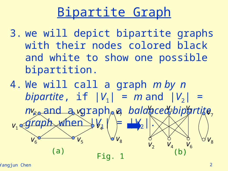
3. we will depict bipartite graphs with their nodes colored black and white to show one possible bipartition.

4. We will call a graph m by n bipartite, if |V1| = m and |V2| = n, and a graph a balanced bipartite graph when |V1| = |V2|.

v1

v2 v3

v4

v5v6

v7

v8

v7

v8

v1 v3 v5

v2 v4 v6

Fig. 1(a) (b)

3Yangjun Chen

Properties

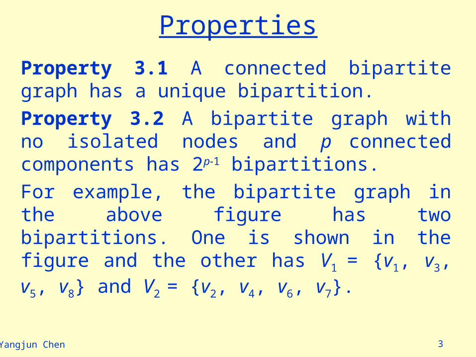
Property 3.1 A connected bipartite graph has a unique bipartition.

Property 3.2 A bipartite graph with no isolated nodes and p connected components has 2p-1 bipartitions.

For example, the bipartite graph in the above figure has two bipartitions. One is shown in the figure and the other has V1 = {v1, v3, v5, v8} and V2

= {v2, v4, v6, v7}.

4Yangjun Chen

PropertiesThe following theorem belongs to König (1916).Theorem 3.3 A graph G is bipartite if and only if G has no cycle of odd length.Corollary 3.4 A connected graph is bipartite if and only if for every node v there is no edge (x, y) such that distance(v, x) = distance(v, y).Corollary 3.5 A graph G is bipartite if and only if it contains no closed walk of odd length.

5Yangjun Chen

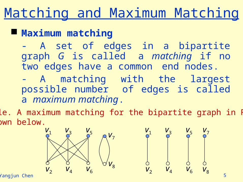
Matching and Maximum Matching Maximum matching

- A set of edges in a bipartite graph G is called a matching if no two edges have a common end nodes.- A matching with the largest possible number of edges is called a maximum matching.

Example. A maximum matching for the bipartite graph in Fig. 1(b)is shown below.

v7

v8

v1 v3 v5

v2 v4 v6

v7

v8

v1 v3 v5

v2 v4 v6

6Yangjun Chen

Maximum Matching Maximum matching

- Many discrete problems can be formulated as problems about maximum matchings. Consider, for

example, probably the most famous:A set of boys each know several girls, is it

possible for the boys each to marry a girl that he knows?This situation has a natural representation as the bipartite graph with bipartition (V1, V2), where V1 is the set of boys, V2 the set of girls, and an edge between a boy and a girl represents that they know one another. The marriage problem is then the problem: does a maximum matching of G have |V1| edges?

7Yangjun Chen

Alternative and Augmenting Path Maximum matching

Let M be a matching of a graph G.- A node v is said to be covered, or saturated by M, if some edges of M is incident with v. We will also call an unsaturated node free.- A path or cycle is alternative, relative to M, if its edges are alternatively in E\M and M.- A path is an augmenting path if it is an alternating path with free origin and terminus.- P - a path. C - a cycle.

|P| - the numbers of edges in P|C| - the numbers of edges in C.

8Yangjun Chen

Properties of Matchings

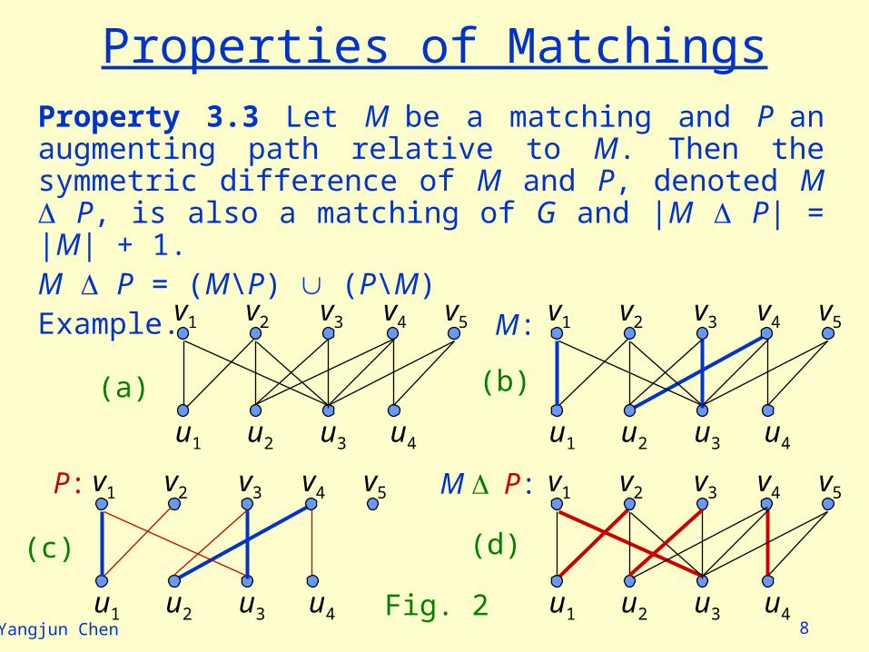
Property 3.3 Let M be a matching and P an augmenting path relative to M. Then the symmetric difference of M and P, denoted M P, is also a matching of G and |M P| = |M| + 1.M P = (M\P) (P\M)Example.

v4

u4

v1 v2 v3

u1 u2 u3

v5v4

u4

v1 v2 v3

u1 u2 u3

v5

v4

u4

v1 v2 v3

u1 u2 u3

v5 v4

u4

v1 v2 v3

u1 u2 u3

v5M:

P: M P:

Fig. 2

(a) (b)

(c) (d)

9Yangjun Chen

Properties of Matchings

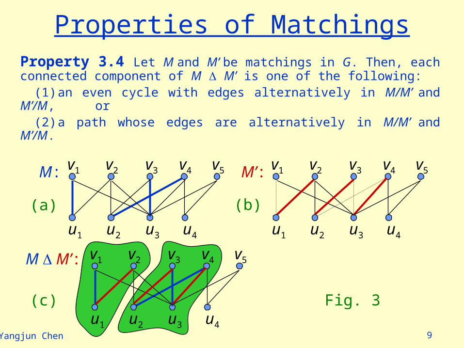
Property 3.4 Let M and M’ be matchings in G. Then, each connected component of M M’ is one of the following:

(1) an even cycle with edges alternatively in M/M’ and M’/M, or

(2) a path whose edges are alternatively in M/M’ and M’/M.

v4

u4

v1 v2 v3

u1 u2 u3

v5M’:v4

u4

v1 v2 v3

u1 u2 u3

v5M:

v4

u4

v1 v2 v3

u1 u2 u3

v5M M’:

Fig. 3

(a) (b)

(c)

10Yangjun Chen

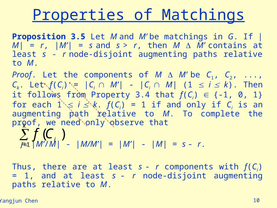
Properties of MatchingsProposition 3.5 Let M and M’ be matchings in G. If |M| = r, |M’| = s and s > r, then M M’ contains at least s - r node-disjoint augmenting paths relative to M.

Proof. Let the components of M M’ be C1, C2, ..., Ck. Let f(Ci) = |Ci M’| - |Ci M| (1 i k). Then it follows from Property 3.4 that f(Ci) {-1, 0, 1} for each 1 i k. f(Ci) = 1 if and only if Ci is an augmenting path relative to M. To complete the proof, we need only observe that

= |M’/M| - |M/M’| = |M’| - |M| = s - r.

Thus, there are at least s - r components with f(Ci) = 1, and at least s - r node-disjoint augmenting paths relative to M.

k

jiCf

1)(

11Yangjun Chen

Properties of MatchingsCombining Proposition 3.5 with Property 3.3, we can deduce the following theorem (Berge, 1957).Theorem 3.6 M is a maximum matching if and only if there is no augmenting path relative to M.The above theorem implies the following property.Property 3.7 If M is a matching of G, then there exists a maximum matching M of G such that the set of nodes covered by M is also covered by M.Proof. If M is a maximum matching, the property trivially holds. Otherwise, consider an augmenting path P relative to M. Then, according to Property 3.1, M P is also a matching of G with

|M P| = |M| + 1.Moreover, the nodes covered by M are also covered by M P. Repeating the above process will prove the property.

12Yangjun Chen

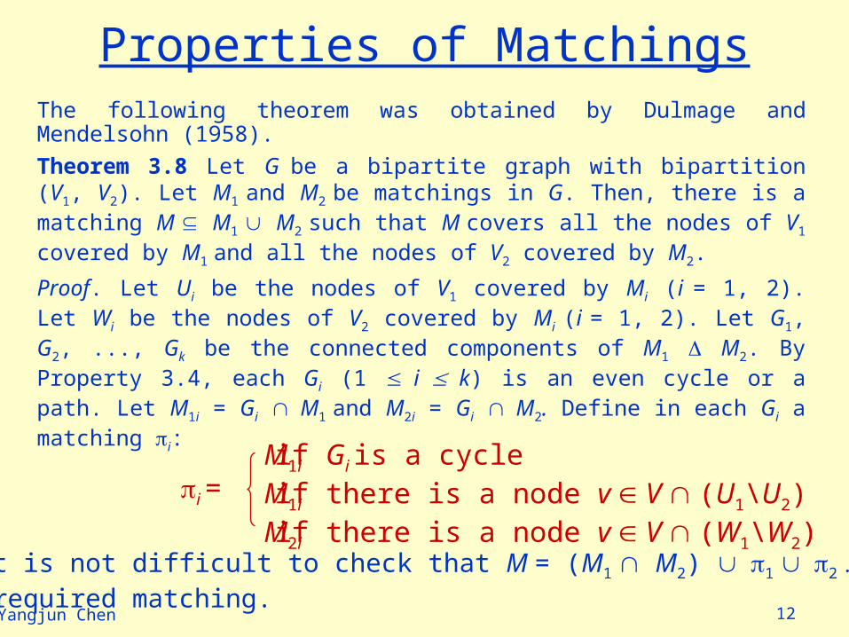
Properties of MatchingsThe following theorem was obtained by Dulmage and Mendelsohn (1958).

Theorem 3.8 Let G be a bipartite graph with bipartition (V1, V2). Let M1 and M2 be matchings in G. Then, there is a matching M M1 M2 such that M covers all the nodes of V1 covered by M1 and all the nodes of V2 covered by M2.

Proof. Let Ui be the nodes of V1 covered by Mi (i = 1, 2). Let Wi be the nodes of V2 covered by Mi (i = 1, 2). Let G1, G2, ..., Gk be the connected components of M1 M2. By Property 3.4, each Gi (1 i k) is an even cycle or a path. Let M1i = Gi M1 and M2i = Gi M2. Define in each Gi a matching i: M1i

M1i

M2i

if Gi is a cycleif there is a node v V (U1\U2)if there is a node v V (W1\W2)

i =

Then, it is not difficult to check that M = (M1 M2) 1 2 k

is the required matching.

13Yangjun Chen

Properties of Matchings

Theorem 3.9 A maximum matching M of a bipartite graph G can be obtained from any other maximum matching M’ by a sequence of transfers along alternating cycles and paths of even length.

Proof. By Property 3.4, every component of M M’ is an alternating even cycle or an alternating path relative to M’. By Property 3.3 and Theorem 3.6, a component of M M’, if it is a path, must be of even length. (Otherwise, if it is an odd path, it must be an augmenting path relative to M or to M’, contradicting the fact that both M and M’ are maximum.) Then, changing M’ in each component in turn will transform M’ into M.

14Yangjun Chen

Properties of Matchings

A perfecting matching of a graph G is a matching which covers every node of G. Clearly, if a graph has two perfect matchings M and M’, all components of M M’ are even cycles. Therefore, according to Theorem 3.9, we can deduce the following result.

Corollary 3.10 Assume that bipartite graph G has a perfect matching M. Then, any other perfect matching can be obtained from M by a sequence of transfers along alternating cycles relative to M.

15Yangjun Chen

Algorithm Algorithms - finding a maximum matching

Lemma 3.11 Let M be a matching with |M| = r and suppose that the cardinality of a maximum matching is s. Then, there exists an augmenting path relative to M of length at most 2 r/(s – r)+ 1.

Proof. Let M’ be a maximum matching. Then, by Proposition 3.5, M M’ contains s - r node-disjoint augmenting paths relative to M. It is easy to see that these paths contain at most r edges from M. So one of them must contain at most r/(s – r) edges from M and so at most 2 r/(s – r) + 1 edges altogether.

16Yangjun Chen

Algorithm

Lemma 3.12 Let M be a matching and P be a shortest augmenting path relative to M. Let Q be an augmenting path relative to M P. Then, |Q| |P| + |P Q|.

Proof. Consider M’ = M P Q. Then, M’ is a matching. By Property 3.3, |M’| = |M P| + 1 = (|M| + 1) + 1 = |M| + 2. According to Proposition 3.5, M M’ contains at least two node-disjoint augmenting paths relative to M. Let P1, ..., Pk (k 2) be such paths. Since P is a shortest augmenting path relative to M, we have

|M M’| = |P Q| |P1| + ... + |Pk| 2|P|.

Note that |P Q| = |P| + |Q| - |P Q| 2|P|. Therefore, we have |Q| |P| + |P Q|.

Note that M’ = M P Q.

17Yangjun Chen

Algorithm

Corollary 3.13 Let P be a shortest augmenting path relative to a matching M, and Q be a shortest augmenting path relative to M P. Then, if |P| = |Q|, the paths P and Q must be node-disjoint. Moreover, Q is also a shortest augmenting path relative to M.Proof. According to Lemma 3.12, we have |P| = |Q| |P| + |P Q|. So P Q = . Thus, P and Q are edge-disjoint. Assume that P and Q share a common node v. Consider the edge e incident with v in M P. Then, P and Q must share e, contradicting P Q = . Therefore, P and Q are also node-disjoint.

18Yangjun Chen

AlgorithmHopcroft-Karp algorithm (1973)The whole computation process is divided into a number of stages, at which some partial matching has been constructed and some way is sought to increase it. At stage i, we have the matching Mi and we search for {Q1, Q2, ..., Qk}, a maximal set of node-disjoint, shortest augmenting paths, relative to Mi. Then, according to Corollary 3.13, Q2 is a shortest augmenting path relative to M Q1, Q3 is a shortest augmenting path relative to (M Q1) Q2, ..., and Qk is a shortest augmenting path relative to (M Q1 Q2 ... Qk-1) Qk.

Therefore, the new matching for the next stage is formed as

Mi+1 = Mi Q1 Q2 ... Qk.

19Yangjun Chen

AlgorithmProposition 3.14 Let s be the cardinality of a maximum matching in a bipartite graph G. Then, to construct a maximum matching by the above process requires at most 2 s1/2 + 2 stages.Proof. It can be derived from Property 3.3 and Lemma 3.11.

Since at each stage at most |E| edges will be accessed, the time complexity of the algorithm is bounded by O(|E|s1/2) = O (|E||V|1/2).

20Yangjun Chen

Algorithm

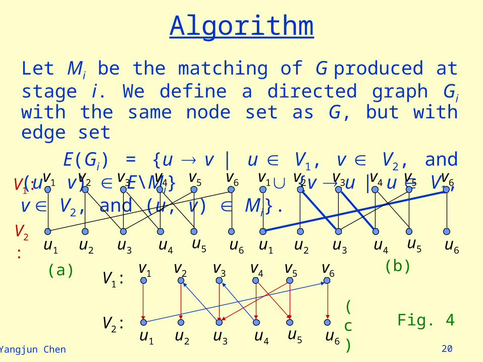
Let Mi be the matching of G produced at stage i. We define a directed graph Gi with the same node set as G, but with edge set

E(Gi) = {u v | u V1, v V2, and (u, v) E\Mi} {v u | u V1, v V2, and (u, v) Mi}.

v4

u4

v1 v2 v3

u1 u2 u3

v5 v6

u5 u6

v4

u4

v1 v2 v3

u1 u2 u3

v5 v6

u5 u6

v4

u4

v1 v2 v3

u1 u2 u3

v5 v6

u5 u6

Fig. 4

(a) (b)

(c)

V1:

V2:

V1:

V2:

21Yangjun Chen

Algorithm

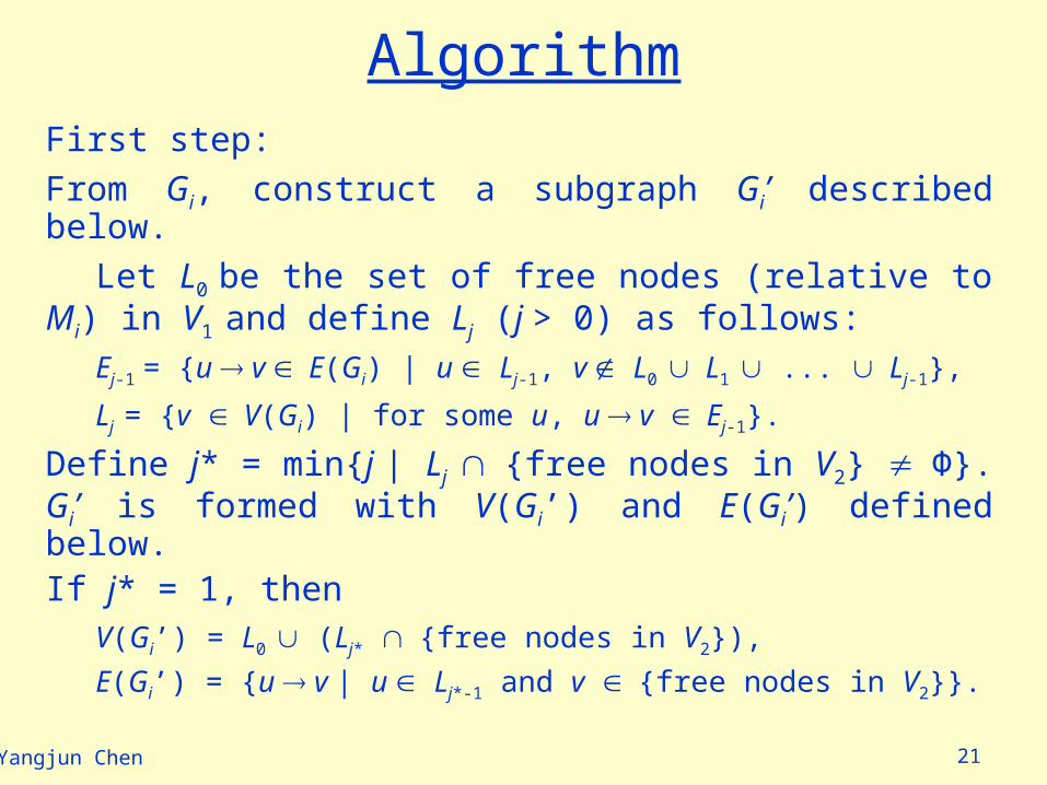
First step:

From Gi, construct a subgraph Gi’ described below.

Let L0 be the set of free nodes (relative to Mi) in V1

and define Lj (j > 0) as follows:

Ej-1 = {u v E(Gi) | u Lj-1, v L0 L1 ... Lj-1},

Lj = {v V(Gi) | for some u, u v Ej-1}.

Define j* = min{j | Lj {free nodes in V2} Ф}. Gi’ is formed with V(Gi’) and E(Gi’) defined below.If j* = 1, then

V(Gi’) = L0 (Lj* {free nodes in V2}),

E(Gi’) = {u v | u Lj*-1 and v {free nodes in V2}}.

22Yangjun Chen

Algorithm

First step:If j* > 1, then

V(Gi’) = L0 L1 ... Lj*-1 (Lj* {free nodes in V2}),

E(Gi’) = E0 E1 ... Ej*-2 {u v | u Lj*-1 and v {free nodes in V2}}.

With this definition of the graph Gi’, directed paths from L0 to Lj* are precisely in one-to-one correspondence with shortest augmenting paths relative to Mi in G.

23Yangjun Chen

Algorithm

Second step:

In this step, we will traverse Gi’ in a depth-first searching fashion to find a maximal set of node-disjoint paths from L0 to Lj*. For this, a stack structure stack is used to control the graph exploring. In addition, we use c-list(v) to represent the set of v’s child nodes.

24Yangjun Chen

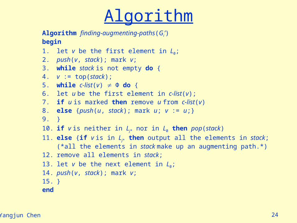
AlgorithmAlgorithm finding-augmenting-paths(Gi’)begin

1. let v be the first element in L0;2. push(v, stack); mark v;3. while stack is not empty do {4. v := top(stack);5. while c-list(v) Ф do {6. let u be the first element in c-list(v);7. if u is marked then remove u from c-list(v)8. else {push(u, stack); mark u; v := u;}9. }

10. if v is neither in Lj* nor in L0 then pop(stack)

11. else {if v is in Lj* then output all the elements in stack;(*all the elements in stack make up an augmenting path.*)

12. remove all elements in stack;

13. let v be the next element in L0;14. push(v, stack); mark v;15. }end

25Yangjun Chen

Example Trace

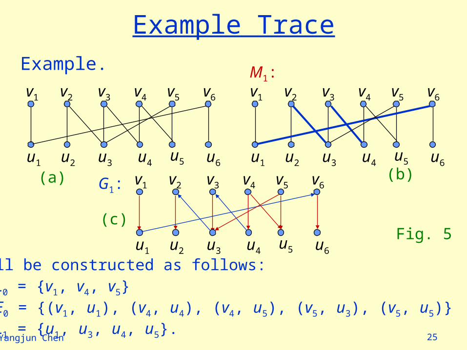
Example.

v4

u4

v1 v2 v3

u1 u2 u3

v5 v6

u5 u6

v4

u4

v1 v2 v3

u1 u2 u3

v5 v6

u5 u6

v4

u4

v1 v2 v3

u1 u2 u3

v5 v6

u5 u6

M1:

G1:

G1’ will be constructed as follows:L0 = {v1, v4, v5}E0 = {(v1, u1), (v4, u4), (v4, u5), (v5, u3), (v5, u5)}L1 = {u1, u3, u4, u5}.

Fig. 5

(a) (b)

(c)

26Yangjun Chen

Example Trace

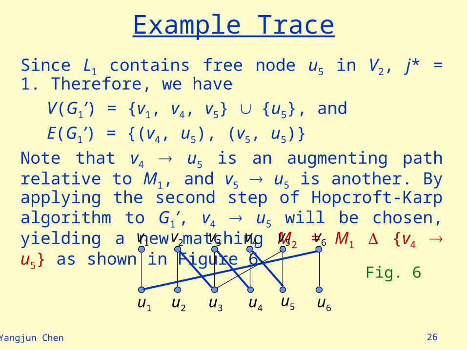
Since L1 contains free node u5 in V2, j* = 1. Therefore, we have

V(G1’) = {v1, v4, v5} {u5}, and

E(G1’) = {(v4, u5), (v5, u5)}

Note that v4 u5 is an augmenting path relative to M1, and v5 u5 is another. By applying the second step of Hopcroft-Karp algorithm to G1’, v4 u5 will be chosen, yielding a new matching M2 = M1 {v4 u5} as shown in Figure 6.

v4

u4

v1 v2 v3

u1 u2 u3

v5 v6

u5 u6

Fig. 6

27Yangjun Chen

Example Trace

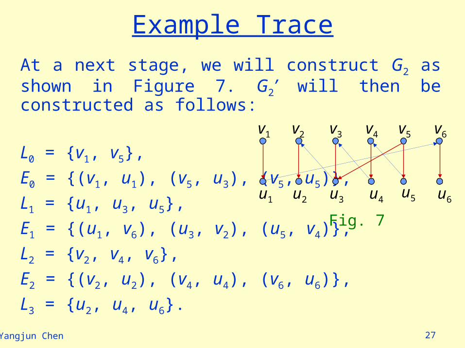
At a next stage, we will construct G2 as shown in Figure 7. G2’ will then be constructed as follows:

L0 = {v1, v5},

E0 = {(v1, u1), (v5, u3), (v5, u5)},

L1 = {u1, u3, u5},

E1 = {(u1, v6), (u3, v2), (u5, v4)},

L2 = {v2, v4, v6},

E2 = {(v2, u2), (v4, u4), (v6, u6)},

L3 = {u2, u4, u6}.

v4

u4

v1 v2 v3

u1 u2 u3

v5 v6

u5 u6

Fig. 7

28Yangjun Chen

Example Trace

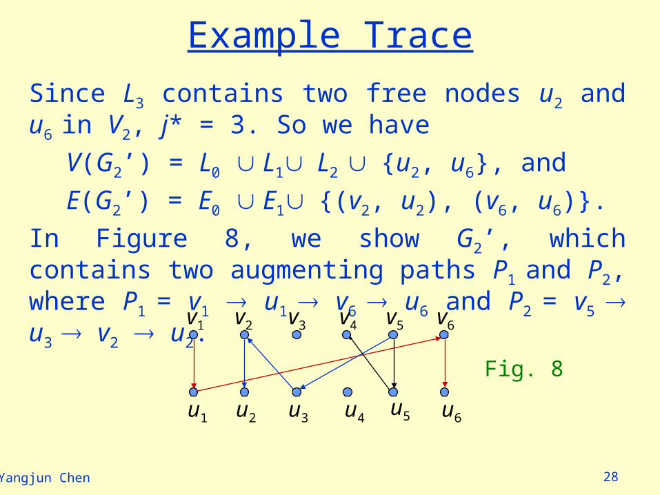
Since L3 contains two free nodes u2 and u6 in V2, j* = 3. So we have

V(G2’) = L0 L1L2 {u2, u6}, and

E(G2’) = E0 E1{(v2, u2), (v6, u6)}.

In Figure 8, we show G2’, which contains two augmenting paths P1 and P2, where P1 = v1 u1 v6 u6 and P2 = v5 u3 v2 u2. v4

u4

v1 v2 v3

u1 u2 u3

v5 v6

u5 u6

Fig. 8

29Yangjun Chen

Example Trace

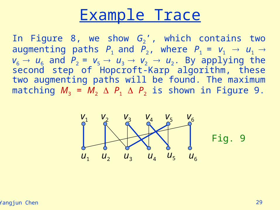
In Figure 8, we show G2’, which contains two augmenting paths P1 and P2, where P1 = v1 u1 v6 u6 and P2 = v5 u3 v2 u2. By applying the second step of Hopcroft-Karp algorithm, these two augmenting paths will be found. The maximum matching M3 = M2 P1 P2 is shown in Figure 9.

v4

u4

v1 v2 v3

u1 u2 u3

v5 v6

u5 u6

Fig. 9

30Yangjun Chen

Example Trace

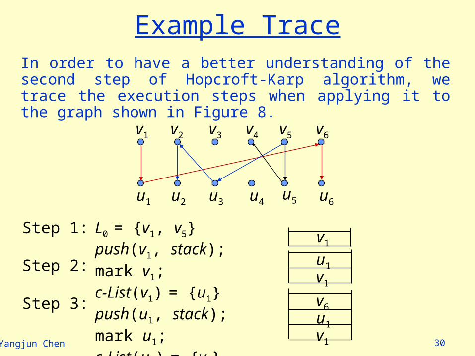
In order to have a better understanding of the second step of Hopcroft-Karp algorithm, we trace the execution steps when applying it to the graph shown in Figure 8.

v4

u4

v1 v2 v3

u1 u2 u3

v5 v6

u5 u6

Step 1:

Step 2:

Step 3:

L0 = {v1, v5}push(v1, stack); mark v1;c-List(v1) = {u1}push(u1, stack); mark u1;c-List(u1) = {v6}push(v6, stack); mark v6;

v1

u1

v1

v6

u1

v1

31Yangjun Chen

v4

u4

v1 v2 v3

u1 u2 u3

v5 v6

u5 u6

Step 4:

Step 5:

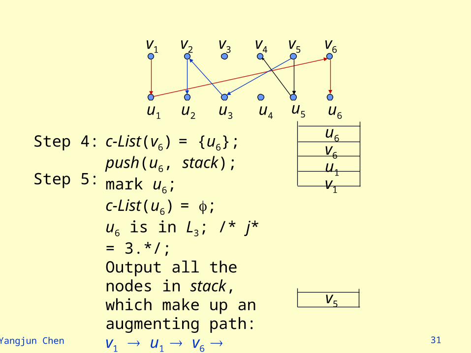
c-List(v6) = {u6};push(u6, stack); mark u6;c-List(u6) = ;u6 is in L3; /* j* = 3.*/;Output all the nodes in stack, which make up an augmenting path:v1 u1 v6 u6 ;empty stack;push(v5, stack); /* v5 is the next element in L0.*/

v5

u6

v6

u1

v1

32Yangjun Chen

v4

u4

v1 v2 v3

u1 u2 u3

v5 v6

u5 u6

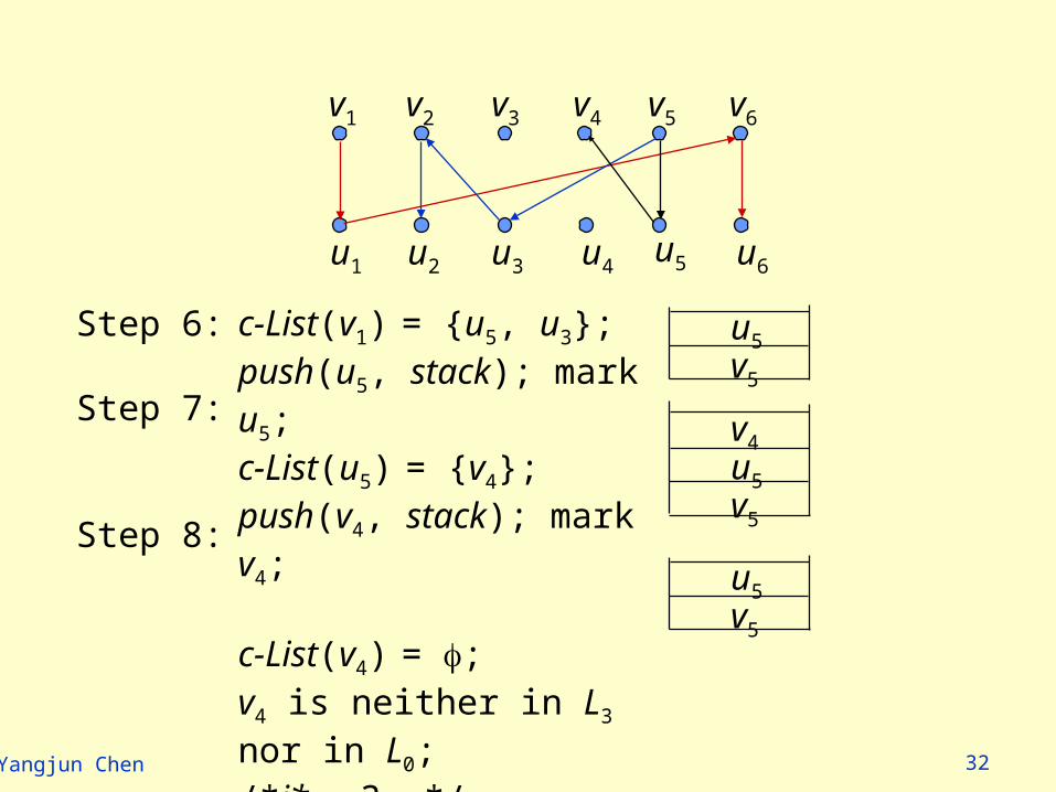
Step 6:

Step 7:

Step 8:

c-List(v1) = {u5, u3};push(u5, stack); mark u5;c-List(u5) = {v4};push(v4, stack); mark v4;

c-List(v4) = ;v4 is neither in L3 nor in L0; /*j* = 3. */pop(stack);

u5

v5

v4

u5

v5

u5

v5

33Yangjun Chen

v4

u4

v1 v2 v3

u1 u2 u3

v5 v6

u5 u6

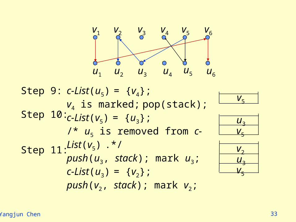
Step 9:

Step 10:

Step 11:

c-List(u5) = {v4};v4 is marked; pop(stack);c-List(v5) = {u3};/* u5 is removed from c-List(v5) .*/push(u3, stack); mark u3;c-List(u3) = {v2};push(v2, stack); mark v2;

u3

v5

v2

u3

v5

v5

34Yangjun Chen

v4

u4

v1 v2 v3

u1 u2 u3

v5 v6

u5 u6

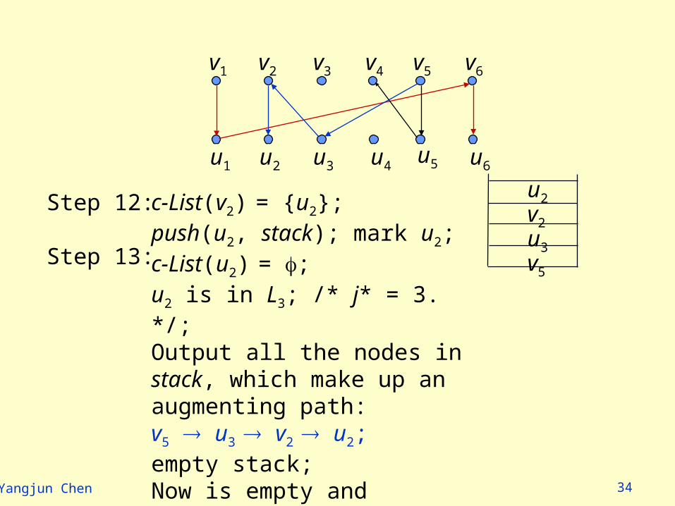
Step 12:

Step 13:

c-List(v2) = {u2};push(u2, stack); mark u2;c-List(u2) = ;u2 is in L3; /* j* = 3. */;Output all the nodes in stack, which make up an augmenting path:v5 u3 v2 u2;empty stack;Now is empty and therefore no element will be pushed into stack. Stop.

u2

v2

u3

v5

35Yangjun Chen

Bipartite Graph

Hopcroft-Karp algorithm (1973)In the above example, we choose the matching shown in Figure 5(b) as an initial matching for ease of explanation. In fact, we can choose any edge in the bipartite graph as an initial matching and then apply Hopcroft-Karp algorithm. Of course, the final matching found may be different from that shown in Figure 9.

36Yangjun Chen

Project Requirement

1. Implementation of the algorithm in C++.

2. Documentation.