Biostatistics: An Introduction

RISE Program 2010

Los Angeles Biomedical Research Institute

at Harbor-UCLA Medical Center

January 15, 2010

Peter D. Christenson

Scientific Decision Making

Setting: Two groups, one gets drug A, one gets placebo (B). Measure outcome.

How do we decide if the drug has an effect?

Perhaps: Say yes if the mean outcome of those receiving drug is greater than the mean of the others?

Outline

Meaning or randomness?

Decisions, truth and errors.

Sensitivity and specificity.

Laws of large numbers.

Experiment size and study power.

Study design considerations.

Resources, software, and references.

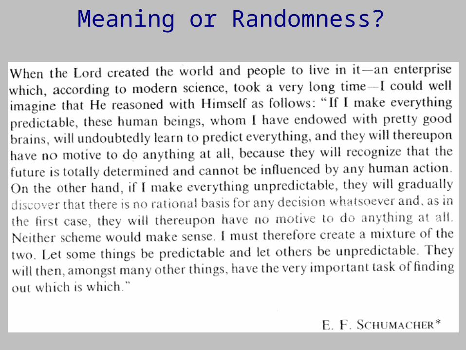
Meaning or Randomness?

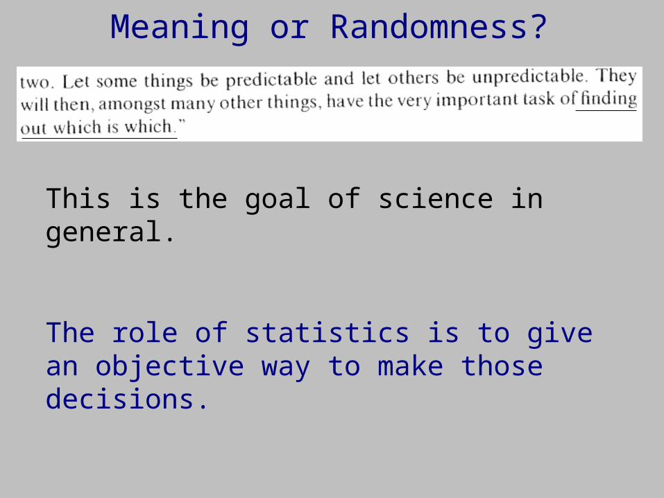
Meaning or Randomness?

This is the goal of science in general.

The role of statistics is to give an objective way to make those decisions.

Meaning or Randomness?

Scientific inferential statistics:

Make a decision: Is it real or random?

Quantify chances that the decision is correct or not.

Other arenas of life:

Suspect guilty? Nobel laureate's opinion?

Make a decision: Is it real or random?

Cannot quantify.

Suppose something “remarkable” happens.

Decision Making

We first discuss using a medical device to make decisions about a patient.

These decisions could be correct or wrong.

We then make an analogy to using an experiment to make decisions about a scientific question.

These decisions could be correct or wrong.

Decision Making: Diagnosis

Mammogram Spot Darkness 100

Definitely Not Cancer

Definitely Cancer

How is the decision made for intermediate darkness?

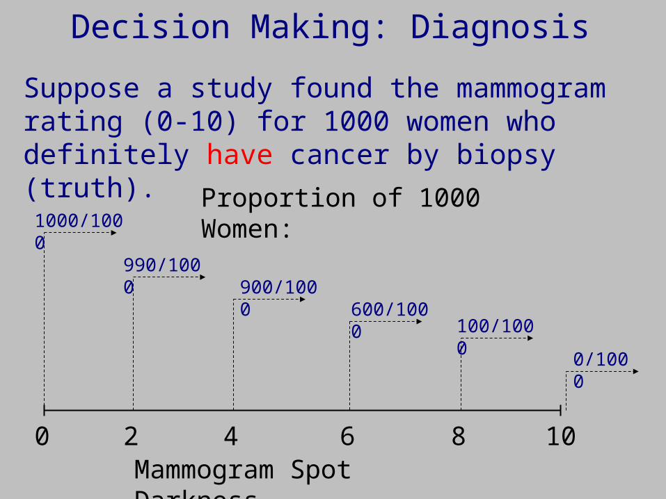
Decision Making: Diagnosis

Mammogram Spot Darkness100

Suppose a study found the mammogram rating (0-10) for 1000 women who definitely have cancer by biopsy (truth).

Proportion of 1000 Women:1000/1000

0/1000

100/1000600/1000

900/1000990/1000

2 4 6 8

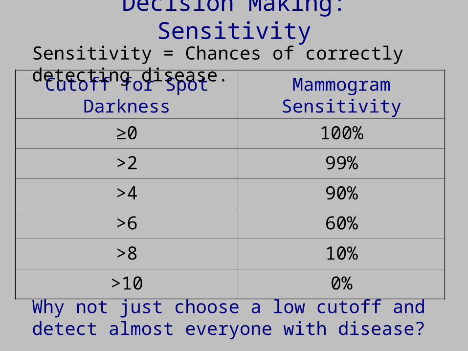
Decision Making: Sensitivity

Cutoff for Spot Darkness Mammogram Sensitivity

≥0 100%

>2 99%

>4 90%

>6 60%

>8 10%

>10 0%

Sensitivity = Chances of correctly detecting disease.

Why not just choose a low cutoff and detect almost everyone with disease?

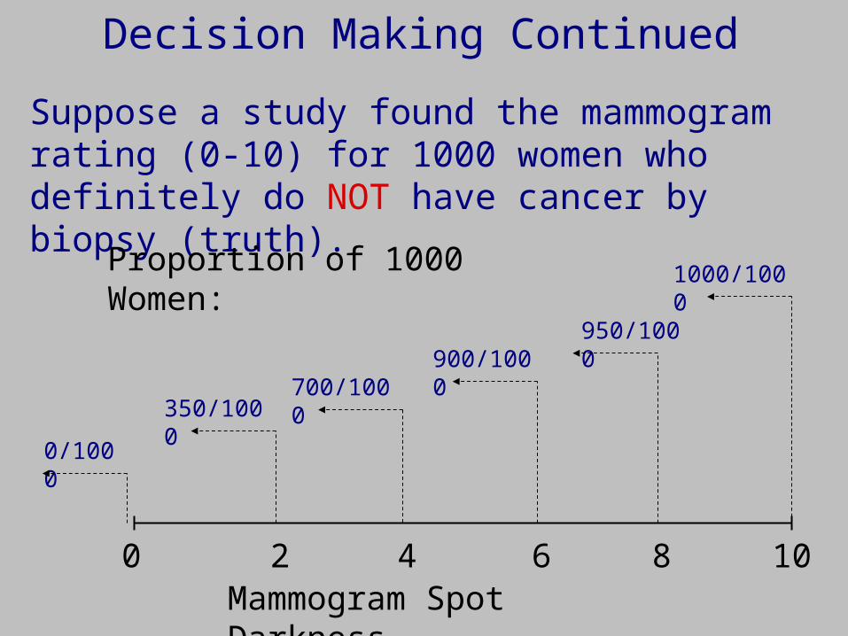
Decision Making Continued

Mammogram Spot Darkness100

Suppose a study found the mammogram rating (0-10) for 1000 women who definitely do NOT have cancer by biopsy (truth).

Proportion of 1000 Women: 1000/1000

0/1000

350/1000700/1000

900/1000950/1000

2 4 6 8

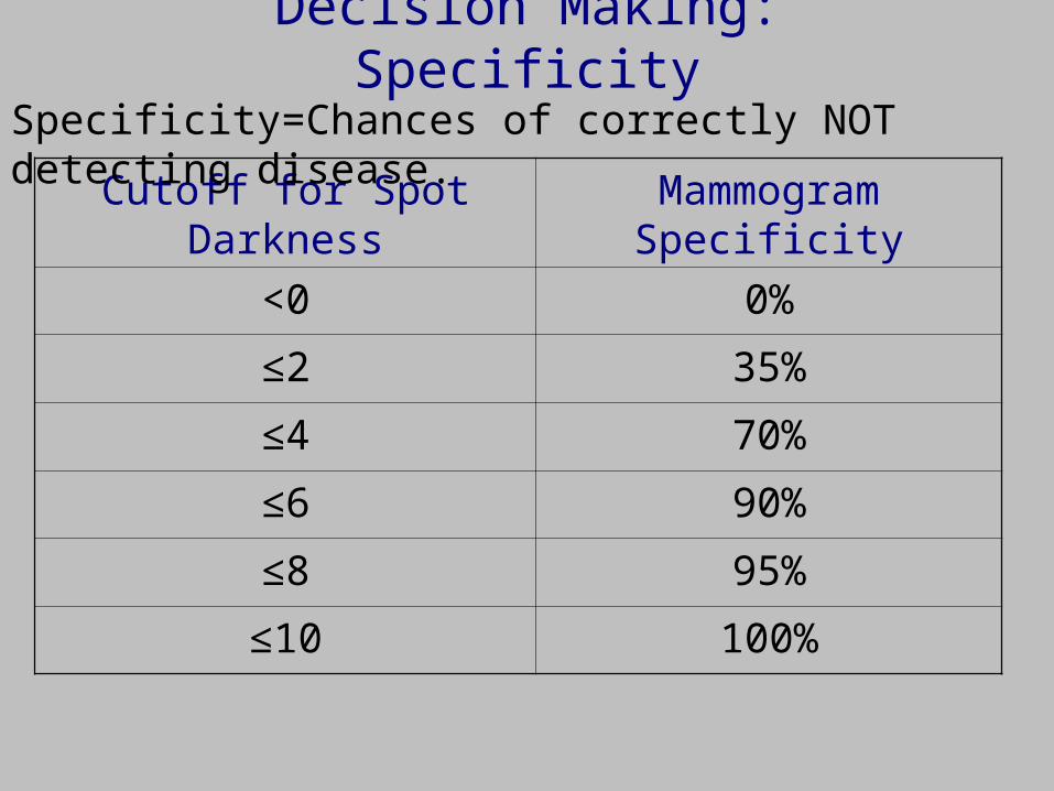
Decision Making: Specificity

Cutoff for Spot Darkness Mammogram Specificity

<0 0%

≤2 35%

≤4 70%

≤6 90%

≤8 95%

≤10 100%

Specificity=Chances of correctly NOT detecting disease.

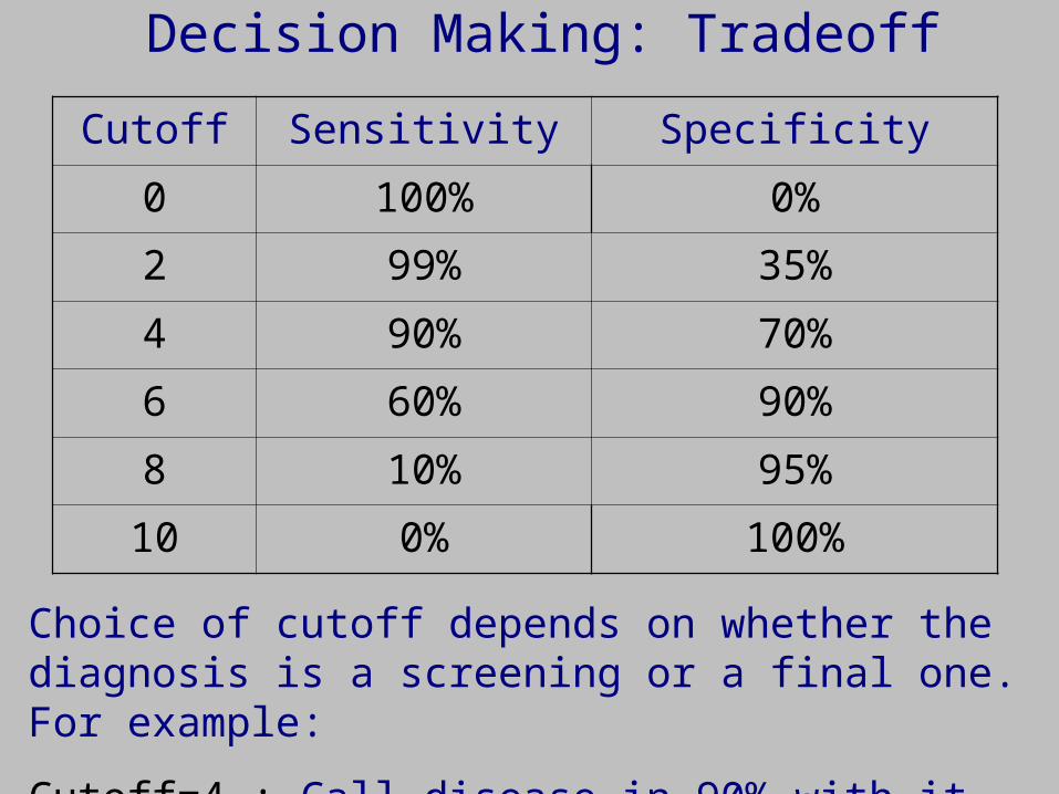
Decision Making: Tradeoff

Cutoff Sensitivity Specificity

0 100% 0%

2 99% 35%

4 90% 70%

6 60% 90%

8 10% 95%

10 0% 100%

Choice of cutoff depends on whether the diagnosis is a screening or a final one. For example:

Cutoff=4 : Call disease in 90% with it and 30% without.

Make Decision: If Spot>6, Decide CA. If Spot≤6, Decide Not CA.

True Non-CA Patients

True CA Patients

Mammogram Spot Darkness0 2 4 6 8 10

\\\ = Specificity = 90%.

/// = Sensitivity = 60%.

Graphical Representation of Tradeoffs

Area under curve =

Probability

Decision Making for Diagnosis: Summary

As sensitivity increases, specificity decreases and vice-versa.

Cannot increase both sensitivity and specificity together.

We now develop sensitivity and specificity to test or decide scientific claims.

True Disease ↔ True claim, real effect.

Decide Disease ↔ Decide claim is true, effect is real.

But, can both increase sensitivity and specificity together.

Scientific Decision Making

Setting: Two groups, one gets drug A, one gets placebo (B). Measure outcome.

How do we decide if the drug has an effect?

Perhaps: Say yes if the mean of those receiving drug is greater than the mean of the others?

Let’s work backwards:

Start with what we want.

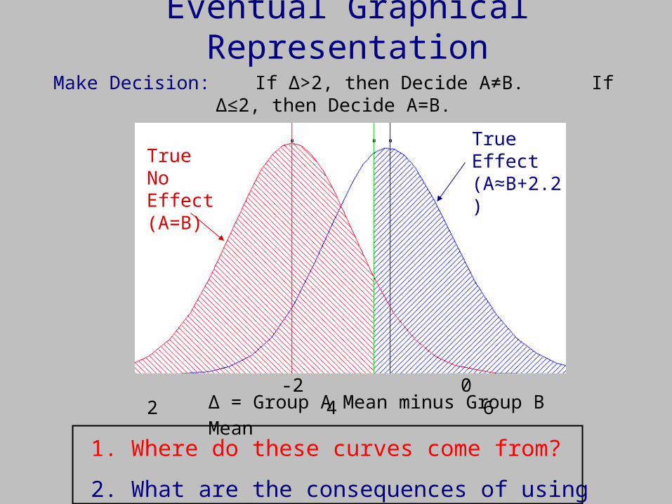
Make Decision: If Δ>2, then Decide A≠B. If Δ≤2, then Decide A=B.

True No Effect (A=B)

True Effect (A≈B+2.2)

Eventual Graphical Representation

1. Where do these curves come from?

2. What are the consequences of using cutoff=2?

Δ = Group A Mean minus Group B Mean -2 0 2 4 6

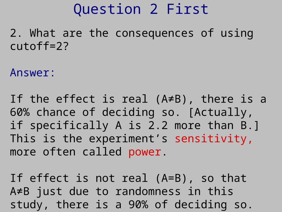
Question 2 First

2. What are the consequences of using cutoff=2?

Answer:

If the effect is real (A≠B), there is a 60% chance of deciding so. [Actually, if specifically A is 2.2 more than B.] This is the experiment’s sensitivity, more often called power.

If effect is not real (A=B), so that A≠B just due to randomness in this study, there is a 90% of deciding so. This is the experiment’s specificity. More often, 100-specificity is called the level of significance.

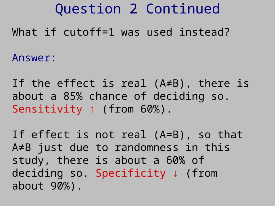
Question 2 Continued

What if cutoff=1 was used instead?

Answer:

If the effect is real (A≠B), there is about a 85% chance of deciding so. Sensitivity ↑ (from 60%).

If effect is not real (A=B), so that A≠B just due to randomness in this study, there is about a 60% of deciding so. Specificity ↓ (from about 90%).

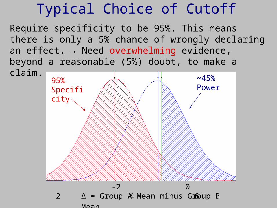
Typical Choice of Cutoff

Δ = Group A Mean minus Group B Mean -2 0 2 4 6

Require specificity to be 95%. This means there is only a 5% chance of wrongly declaring an effect. → Need overwhelming evidence, beyond a reasonable (5%) doubt, to make a claim.

~45% Power

95% Specificity

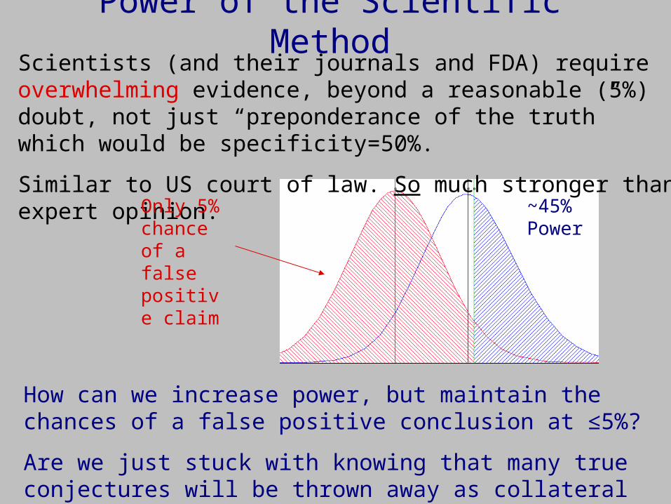
Power of the Scientific MethodScientists (and their journals and FDA) require overwhelming evidence, beyond a reasonable (5%) doubt, not just “preponderance of the truth” which would be specificity=50%.

Similar to US court of law. So much stronger than expert opinion.

~45% Power

Only 5% chance of a false positive claim

How can we increase power, but maintain the chances of a false positive conclusion at ≤5%?

Are we just stuck with knowing that many true conjectures will be thrown away as collateral damage to this rigor?

Back to Question 1

1. Where do the curves in the last figure come from?

Answer:

You specify three quantities: (1) where their peaks are (the experiment’s detectable difference), and how wide they are (determined by (2) natural variation and (3) the # of subjects or animals or tissue samples, N).

Those specifications give a unique set of “bell-shaped” curves. How?

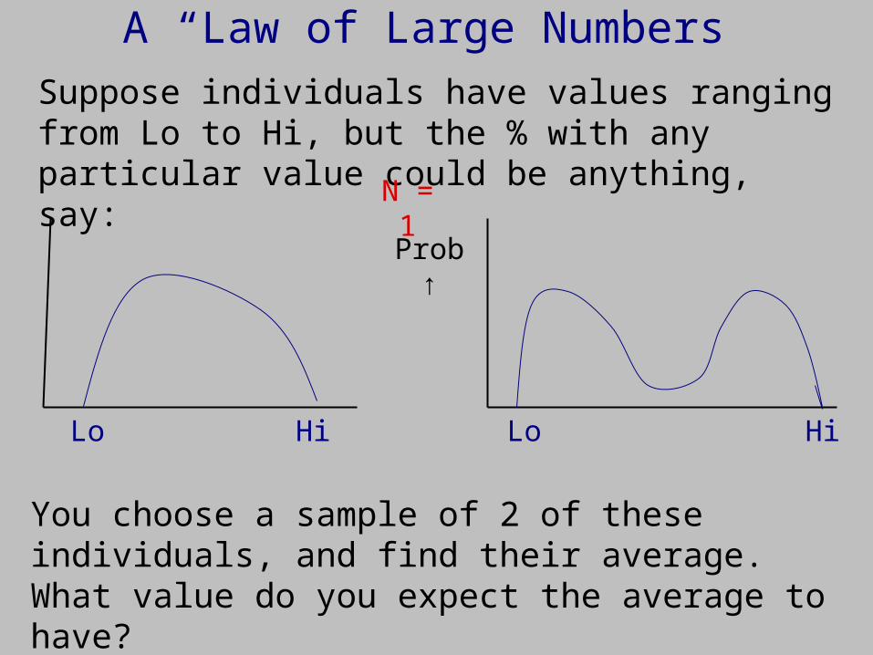
A “Law of Large Numbers”

Suppose individuals have values ranging from Lo to Hi, but the % with any particular value could be anything, say:

You choose a sample of 2 of these individuals, and find their average. What value do you expect the average to have?

Lo LoHi Hi

Prob ↑

N = 1

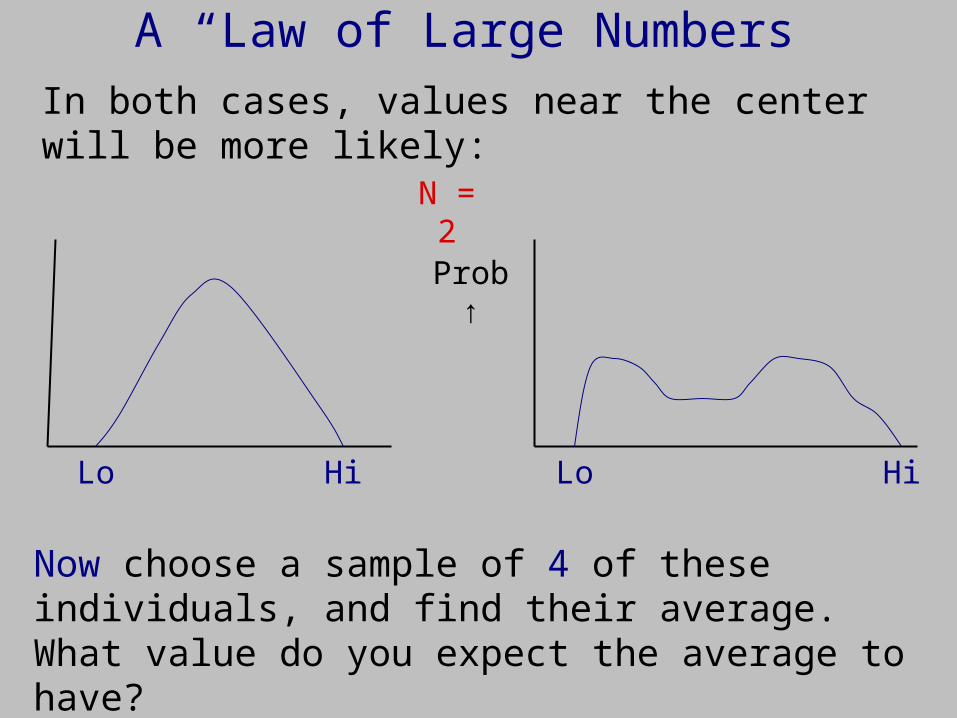
A “Law of Large Numbers”

In both cases, values near the center will be more likely:

Now choose a sample of 4 of these individuals, and find their average. What value do you expect the average to have?

Lo LoHi Hi

Prob ↑

N = 2

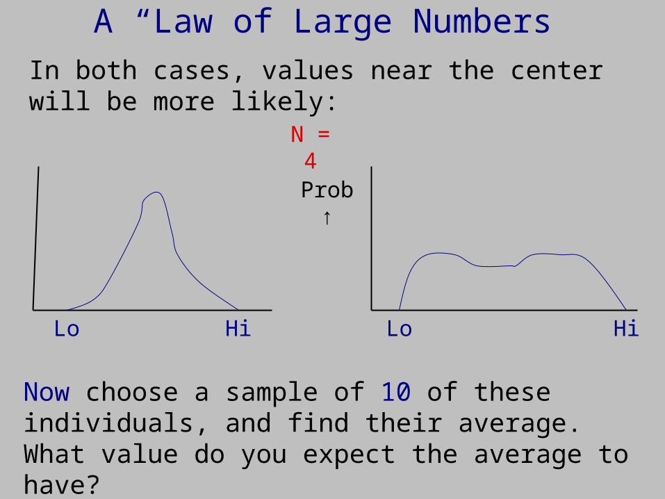
A “Law of Large Numbers”

In both cases, values near the center will be more likely:

Now choose a sample of 10 of these individuals, and find their average. What value do you expect the average to have?

Lo LoHi Hi

Prob ↑

N = 4

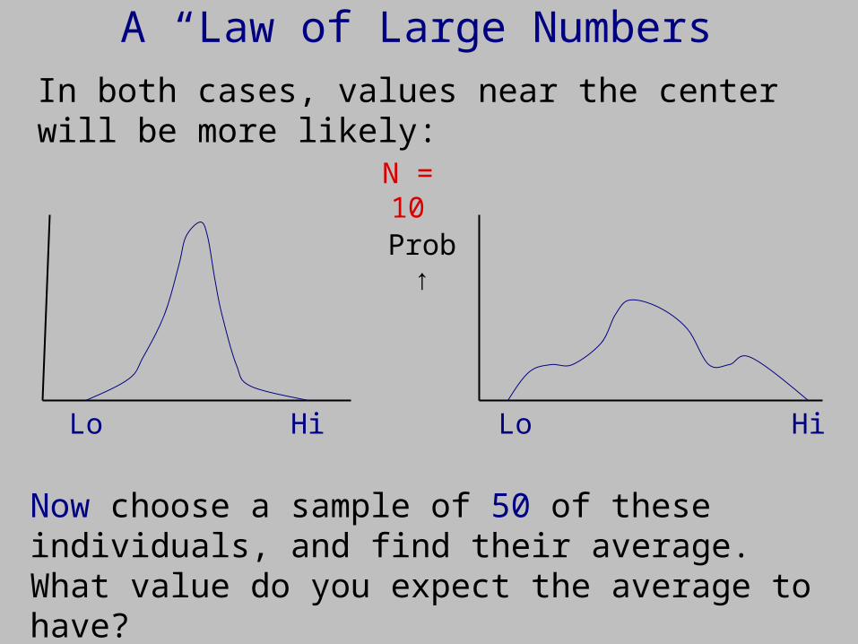
A “Law of Large Numbers”

In both cases, values near the center will be more likely:

Now choose a sample of 50 of these individuals, and find their average. What value do you expect the average to have?

Lo LoHi Hi

Prob ↑

N = 10

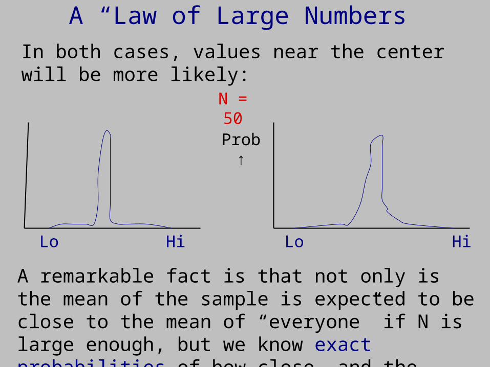
A “Law of Large Numbers”

In both cases, values near the center will be more likely:

A remarkable fact is that not only is the mean of the sample is expected to be close to the mean of “everyone” if N is large enough, but we know exact probabilities of how close, and the shape of the curve.

Lo LoHi Hi

Prob ↑

N = 50

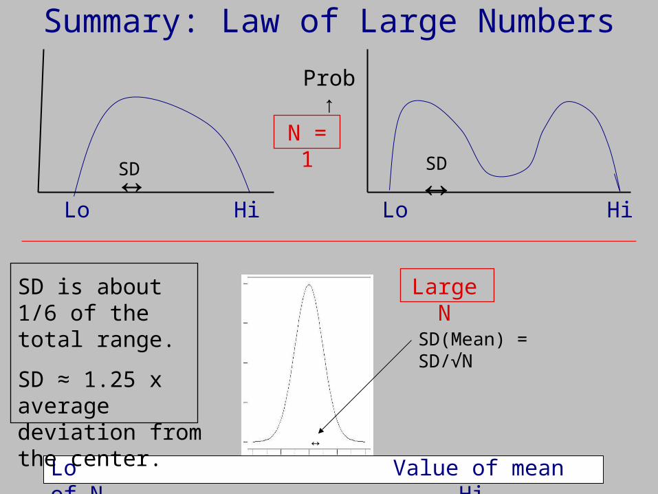
Summary: Law of Large Numbers

Lo LoHi Hi

Prob ↑

N = 1

SD↔ ↔SD

Lo Value of mean of N Hi↔

SD(Mean) = SD/√N

SD is about 1/6 of the total range.

SD ≈ 1.25 x average deviation from the center.

Large N

Scientific Decision Making

So, where are we?

We can now answer the basic dilemma we raised. Repeat earlier slide:

The Power of the Scientific MethodScientists (and their journals and FDA) require overwhelming evidence, beyond a reasonable (5%) doubt, not just “preponderance of the truth” which would be specificity=50%.

Similar to US court of law. So much stronger than expert opinion.

~45% Power

Only 5% chance of a false positive claim

How can we increase power, but maintain the chances of a false positive conclusion at ≤5%?

Are we just stuck with knowing that many true conjectures will be thrown away as collateral damage to this rigor?

N ≈ 170

Scientific Decision Making

So, the answer to the basic dilemma is that by choosing N large enough, we get more precise means, which narrow the curves, which increases the study power.

We can thus find true effects with high certainty, say 80%, and also not claim false effects very often (5%):

Only 5% chance of a false positive claim

80% Power

N ≈ 380

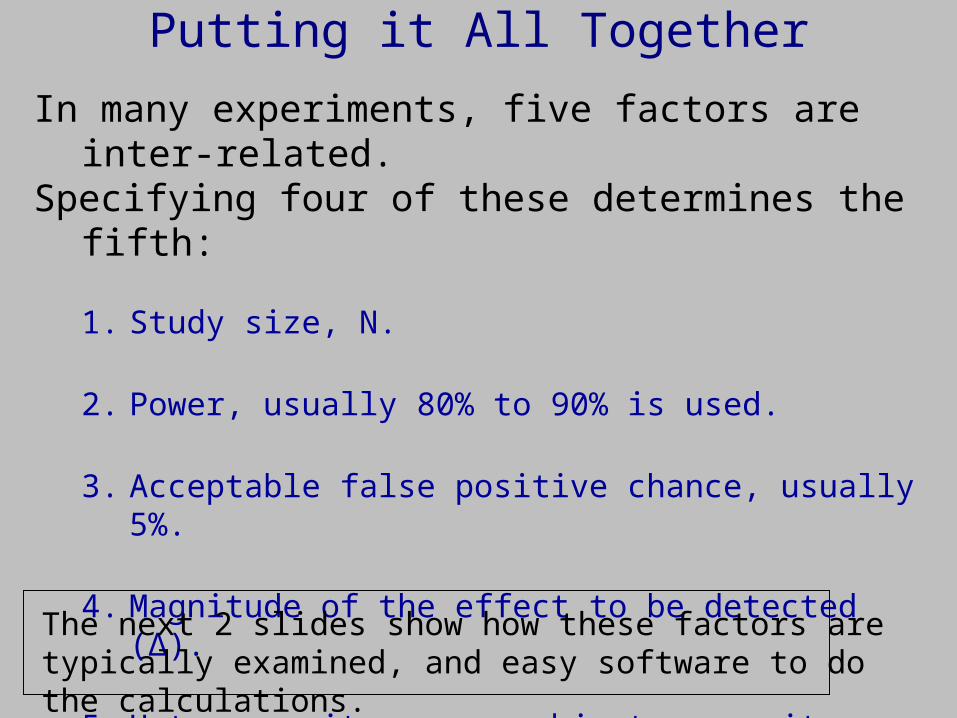
In many experiments, five factors are inter-related. Specifying four of these determines the fifth:

1. Study size, N.

2. Power, usually 80% to 90% is used.

3. Acceptable false positive chance, usually 5%.

4. Magnitude of the effect to be detected (Δ).

5. Heterogeneity among subjects or units (SD).

The next 2 slides show how these factors are typically examined, and easy software to do the calculations.

Putting it All Together

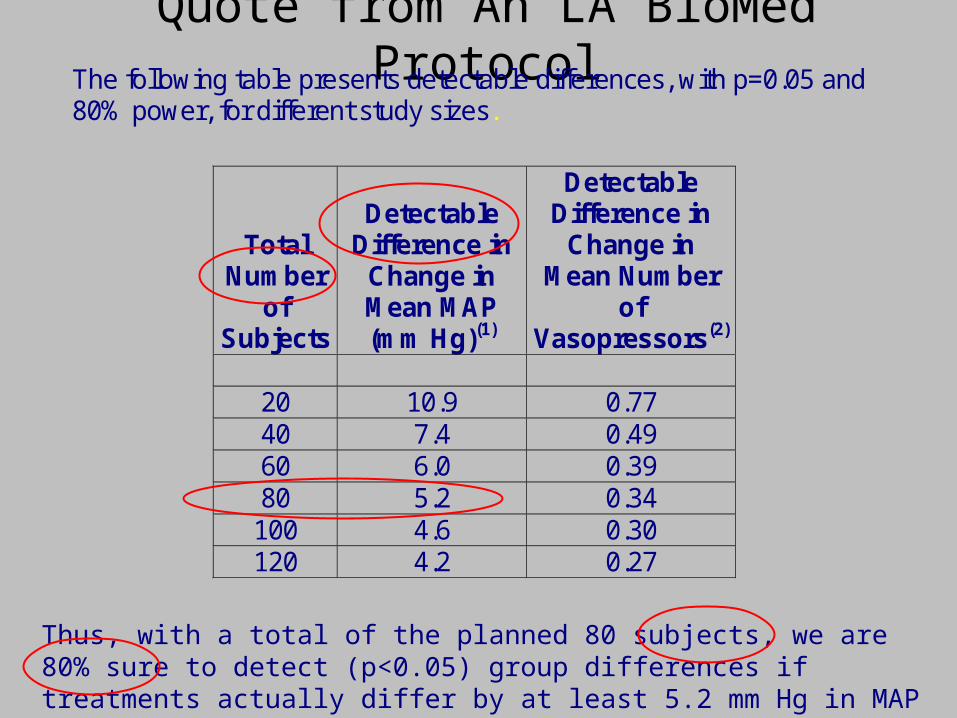
Quote from An LA BioMed ProtocolThe following table presents detectable differences, with p=0.05 and 80% power, for different study sizes.

Total Number

of Subjects

Detectable Difference in

Change in Mean MAP (mm Hg)(1)

Detectable Difference in

Change in Mean Number

of Vasopressors(2)

20 10.9 0.77 40 7.4 0.49 60 6.0 0.39 80 5.2 0.34 100 4.6 0.30 120 4.2 0.27

Thus, with a total of the planned 80 subjects, we are 80% sure to detect (p<0.05) group differences if treatments actually differ by at least 5.2 mm Hg in MAP change, or by a mean 0.34 change in number of vasopressors.

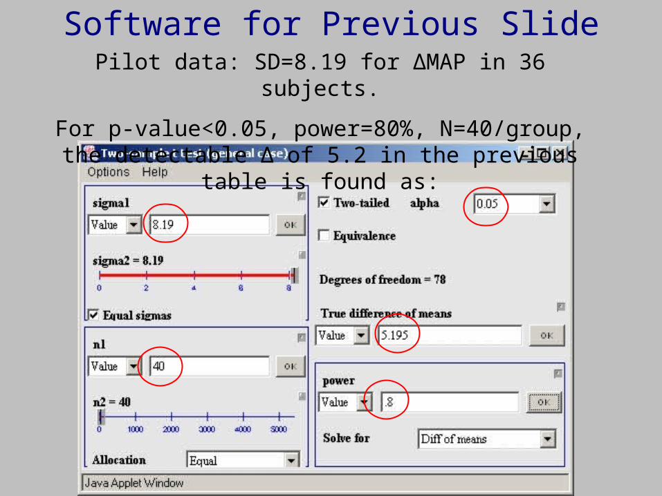
Software for Previous SlidePilot data: SD=8.19 for ΔMAP in 36 subjects.

For p-value<0.05, power=80%, N=40/group, the detectable Δ of 5.2 in the previous table is found as:

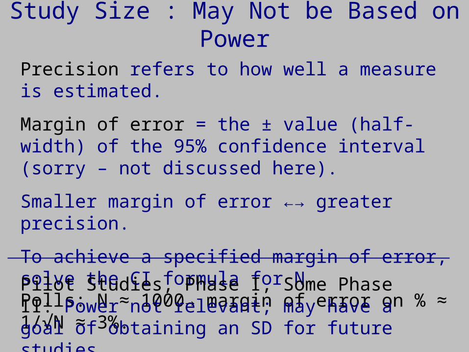
Study Size : May Not be Based on Power

Precision refers to how well a measure is estimated.

Margin of error = the ± value (half-width) of the 95% confidence interval (sorry – not discussed here).

Smaller margin of error ←→ greater precision.

To achieve a specified margin of error, solve the CI formula for N.Polls: N ≈ 1000→ margin of error on % ≈ 1/√N ≈ 3%.

Pilot Studies, Phase I, Some Phase II: Power not relevant; may have a goal of obtaining an SD for future studies.

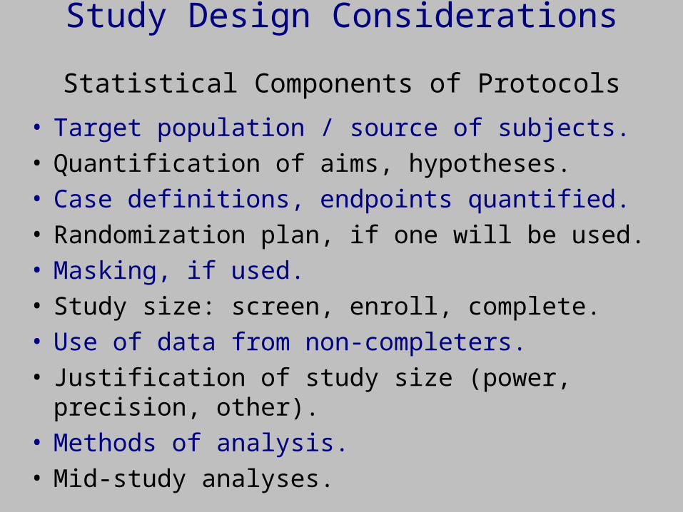
Study Design Considerations Statistical Components of Protocols

• Target population / source of subjects.• Quantification of aims, hypotheses.• Case definitions, endpoints quantified. • Randomization plan, if one will be used.• Masking, if used.• Study size: screen, enroll, complete.• Use of data from non-completers.• Justification of study size (power, precision, other).• Methods of analysis.• Mid-study analyses.

Resources, Software, and References

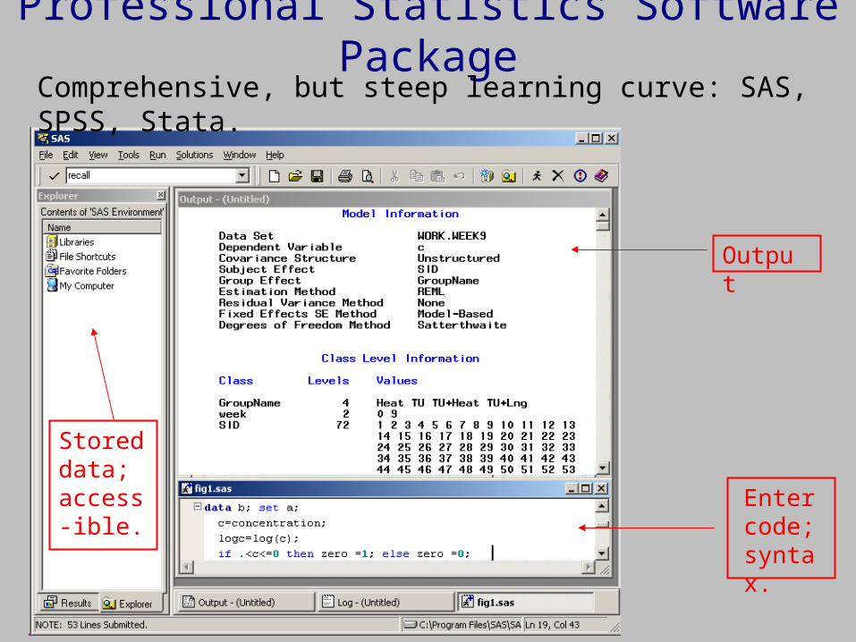
Professional Statistics Software Package

Output

Enter code; syntax.

Stored data; access-ible.

Comprehensive, but steep learning curve: SAS, SPSS, Stata.

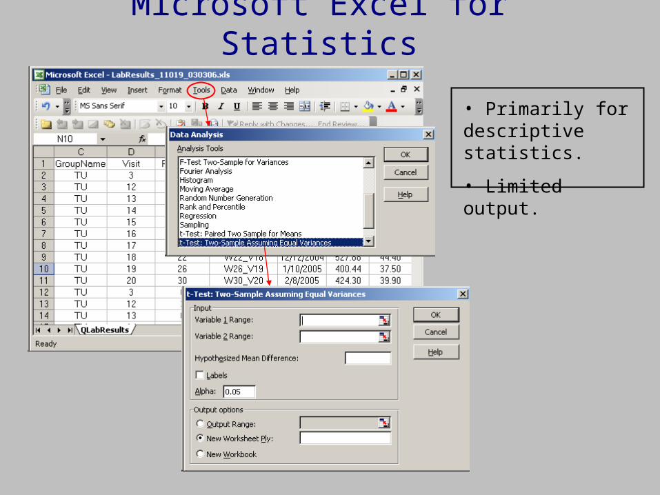
Microsoft Excel for Statistics

• Primarily for descriptive statistics.

• Limited output.

Typical Statistics Software PackageSelect Methods from Menus

Output after menu selection

Data in spreadsheet

www.ncss.com

www.minitab.com

www.stata.com

$100 - $500

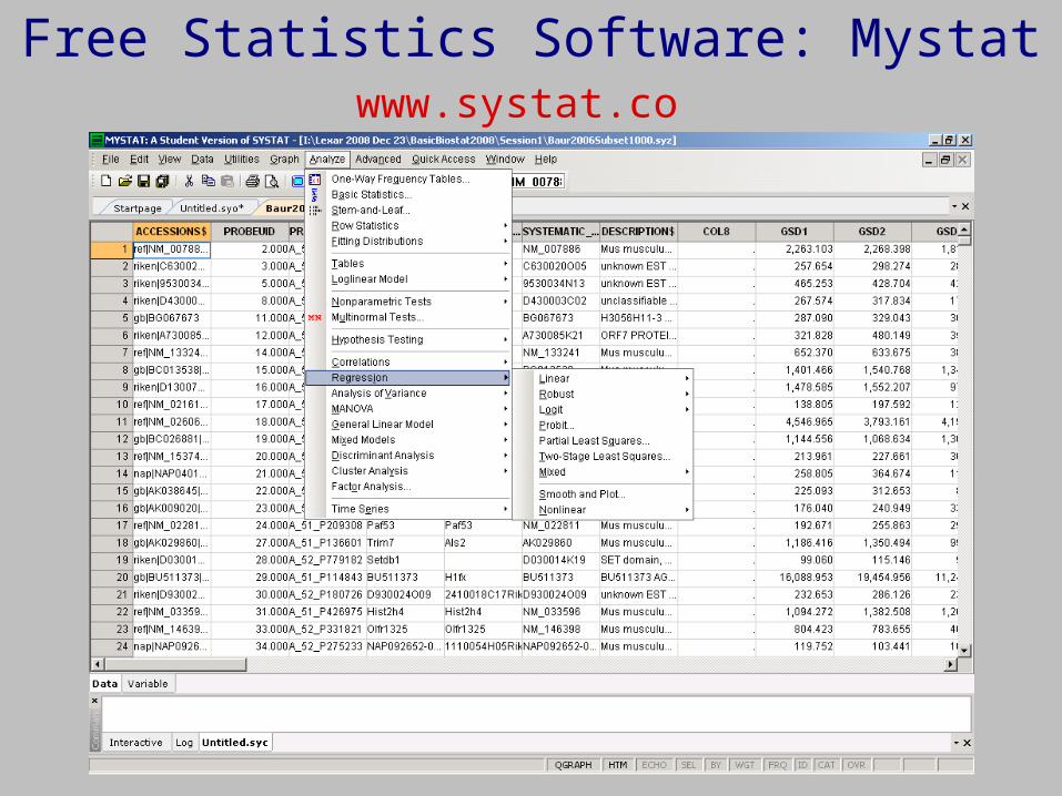
Free Statistics Software: Mystatwww.systat.com

Free Study Size Software

www.stat.uiowa.edu/~rlenth/Power

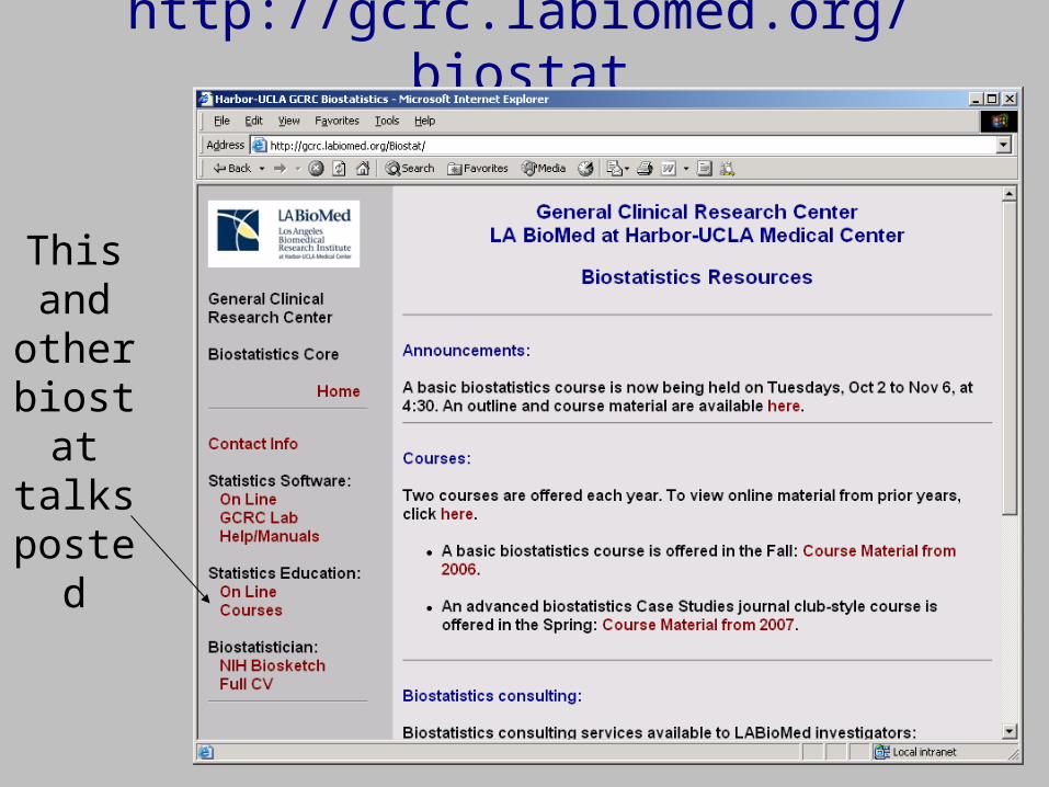
http://gcrc.labiomed.org/biostat

This and

other biostat talks

posted

Recommended Textbook: Making Inference

Design issues

Biases

How to read papers

Meta-analyses

Dropouts

Non-mathematical

Many examples

Thank You

Nils Simonson, in

Furberg & Furberg,

Evaluating Clinical Research