The International Journal of Biostatistics -...

Volume 6, Issue 2 2010 Article 7

The International Journal ofBiostatistics

CAUSAL INFERENCE

An Introduction to Causal Inference

Judea Pearl, University of California, Los Angeles

Recommended Citation:Pearl, Judea (2010) "An Introduction to Causal Inference," The International Journal ofBiostatistics: Vol. 6: Iss. 2, Article 7.DOI: 10.2202/1557-4679.1203Available at: http://www.bepress.com/ijb/vol6/iss2/7

©2010 Berkeley Electronic Press. All rights reserved.

TECHNICAL REPORT R-354

March 2011

An Introduction to Causal InferenceJudea Pearl

Abstract

This paper summarizes recent advances in causal inference and underscores the paradigmaticshifts that must be undertaken in moving from traditional statistical analysis to causal analysis ofmultivariate data. Special emphasis is placed on the assumptions that underlie all causalinferences, the languages used in formulating those assumptions, the conditional nature of allcausal and counterfactual claims, and the methods that have been developed for the assessment ofsuch claims. These advances are illustrated using a general theory of causation based on theStructural Causal Model (SCM) described in Pearl (2000a), which subsumes and unifies otherapproaches to causation, and provides a coherent mathematical foundation for the analysis ofcauses and counterfactuals. In particular, the paper surveys the development of mathematical toolsfor inferring (from a combination of data and assumptions) answers to three types of causalqueries: those about (1) the effects of potential interventions, (2) probabilities of counterfactuals,and (3) direct and indirect effects (also known as "mediation"). Finally, the paper defines theformal and conceptual relationships between the structural and potential-outcome frameworks andpresents tools for a symbiotic analysis that uses the strong features of both. The tools aredemonstrated in the analyses of mediation, causes of effects, and probabilities of causation.

KEYWORDS: structural equation models, confounding, graphical methods, counterfactuals,causal effects, potential-outcome, mediation, policy evaluation, causes of effects

Author Notes: Portions of this paper are adapted from Pearl (2000a, 2009a,b); I am indebted toElja Arjas, Sander Greenland, David MacKinnon, Patrick Shrout, and many readers of the UCLACausality Blog (http://www.mii.ucla.edu/causality/) for reading and commenting on varioussegments of this manuscript, and especially to Erica Moodie and David Stephens for theirthorough editorial input. This research was supported in parts by NIH grant #1R01 LM009961-01,NSF grant #IIS-0914211, and ONR grant #N000-14-09-1-0665.

1 Introduction

Most studies in the health, social and behavioral sciences aim to answer causal

rather than associative – questions. Such questions require some knowledge of the

data-generating process, and cannot be computed from the data alone, nor from the

distributions that govern the data. Remarkably, although much of the conceptual

framework and algorithmic tools needed for tackling such problems are now well

established, they are not known to many of the researchers who could put them

into practical use. Solving causal problems systematically requires certain exten-

sions in the standard mathematical language of statistics, and these extensions are

not typically emphasized in the mainstream literature. As a result, many statistical

researchers have not yet benefited from causal inference results in (i) counterfac-

tual analysis, (ii) nonparametric structural equations, (iii) graphical models, and (iv)

the symbiosis between counterfactual and graphical methods. This survey aims at

making these contemporary advances more accessible by providing a gentle intro-

duction to causal inference for a more in-depth treatment and its methodological

principles (see (Pearl, 2000a, 2009a,b)).

In Section 2, we discuss coping with untested assumptions and new math-

ematical notation which is required to move from associational to causal statistics.

Section 3.1 introduces the fundamentals of the structural theory of causation and

uses these modeling fundamentals to represent interventions and develop mathe-

matical tools for estimating causal effects (Section 3.3) and counterfactual quanti-

ties (Section 3.4). Section 4 outlines a general methodology to guide problems of

causal inference: Define, Assume, Identify and Estimate, with each step benefiting

from the tools developed in Section 3.

Section 5 relates these tools to those used in the potential-outcome frame-

work, and offers a formal mapping between the two frameworks and a symbiosis

(Section 5.3) that exploits the best features of both. Finally, the benefit of this

symbiosis is demonstrated in Section 6, in which the structure-based logic of coun-

terfactuals is harnessed to estimate causal quantities that cannot be defined within

the paradigm of controlled randomized experiments. These include direct and indi-

rect effects, the effect of treatment on the treated, and questions of attribution, i.e.,

whether one event can be deemed “responsible” for another.

1

Pearl: An Introduction to Causal Inference

Published by Berkeley Electronic Press, 2010

2 From Association to Causation

2.1 Understanding the distinction and its implications

The aim of standard statistical analysis is to assess parameters of a distribution from

samples drawn of that distribution. With the help of such parameters, associations

among variables can be inferred, which permits the researcher to estimate prob-

abilities of past and future events and update those probabilities in light of new

information. These tasks are managed well by standard statistical analysis so long

as experimental conditions remain the same. Causal analysis goes one step further;

its aim is to infer probabilities under conditions that are changing, for example,

changes induced by treatments or external interventions.

This distinction implies that causal and associational concepts do not mix;

there is nothing in a distribution function to tell us how that distribution would dif-

fer if external conditions were to change—say from observational to experimental

setup—because the laws of probability theory do not dictate how one property of a

distribution ought to change when another property is modified. This information

must be provided by causal assumptions which identify relationships that remain

invariant when external conditions change.

A useful demarcation line between associational and causal concepts crisp

and easy to apply, can be formulated as follows. An associational concept is any

relationship that can be defined in terms of a joint distribution of observed vari-

ables, and a causal concept is any relationship that cannot be defined from the

distribution alone. Examples of associational concepts are: correlation, regres-

sion, dependence, conditional independence, likelihood, collapsibility, propensity

score, risk ratio, odds ratio, marginalization, conditionalization, “controlling for,”

and many more. Examples of causal concepts are: randomization, influence, effect,

confounding, “holding constant,” disturbance, error terms, structural coefficients,

spurious correlation, faithfulness/stability, instrumental variables, intervention, ex-

planation, and attribution. The former can, while the latter cannot be defined in

term of distribution functions.

This demarcation line is extremely useful in tracing the assumptions that are

needed for substantiating various types of scientific claims. Every claim invoking

causal concepts must rely on some premises that invoke such concepts; it cannot be

inferred from, or even defined in terms statistical associations alone.

This distinction further implies that causal relations cannot be expressed in

the language of probability and, hence, that any mathematical approach to causal

analysis must acquire new notation – probability calculus is insufficient. To illus-

trate, the syntax of probability calculus does not permit us to express the simple fact

that “symptoms do not cause diseases,” let alone draw mathematical conclusions

2

The International Journal of Biostatistics, Vol. 6 [2010], Iss. 2, Art. 7

http://www.bepress.com/ijb/vol6/iss2/7DOI: 10.2202/1557-4679.1203

from such facts. All we can say is that two events are dependent—meaning that if

we find one, we can expect to encounter the other, but we cannot distinguish sta-

tistical dependence, quantified by the conditional probability P(disease|symptom)from causal dependence, for which we have no expression in standard probability

calculus.

2.2 Untested assumptions and new notation

The preceding two requirements: (1) to commence causal analysis with untested,1

theoretically or judgmentally based assumptions, and (2) to extend the syntax of

probability calculus, constitute the two primary barriers to the acceptance of causal

analysis among professionals with traditional training in statistics.

Associational assumptions, even untested, are testable in principle, given

sufficiently large sample and sufficiently fine measurements. Causal assumptions,

in contrast, cannot be verified even in principle, unless one resorts to experimental

control. This difference stands out in Bayesian analysis. Though the priors that

Bayesians commonly assign to statistical parameters are untested quantities, the

sensitivity to these priors tends to diminish with increasing sample size. In contrast,

sensitivity to prior causal assumptions, say that treatment does not change gender,

remains substantial regardless of sample size.

This makes it doubly important that the notation we use for expressing

causal assumptions be cognitively meaningful and unambiguous so that one can

clearly judge the plausibility or inevitability of the assumptions articulated. Statis-

ticians can no longer ignore the mental representation in which scientists store expe-

riential knowledge, since it is this representation, and the language used to access it

that determine the reliability of the judgments upon which the analysis so crucially

depends.

Those versed in the potential-outcome notation (Neyman, 1923, Rubin, 1974,

Holland, 1988), can recognize causal expressions through the subscripts that are at-

tached to counterfactual events and variables, e.g. Yx(u) or Zxy. (Some authors use

parenthetical expressions, e.g. Y (0), Y(1), Y (x,u) or Z(x,y).) The expression Yx(u),for example, stands for the value that outcome Y would take in individual u, had

treatment X been at level x. If u is chosen at random, Yx is a random variable, and

one can talk about the probability that Yx would attain a value y in the population,

written P(Yx = y) (see Section 5 for semantics). Alternatively, Pearl (1995) used

expressions of the form P(Y = y|set(X = x)) or P(Y = y|do(X = x)) to denote the

probability (or frequency) that event (Y = y) would occur if treatment condition

1By “untested” I mean untested using frequency data in nonexperimental studies.

3



X = x were enforced uniformly over the population.2 Still a third notation that dis-

tinguishes causal expressions is provided by graphical models, where the arrows

convey causal directionality.

However, few have taken seriously the textbook requirement that any in-

troduction of new notation must entail a systematic definition of the syntax and

semantics that governs the notation. Moreover, in the bulk of the statistical litera-

ture before 2000, causal claims rarely appear in the mathematics. They surface only

in the verbal interpretation that investigators occasionally attach to certain associ-

ations, and in the verbal description with which investigators justify assumptions.

For example, the assumption that a covariate not be affected by a treatment, a nec-

essary assumption for the control of confounding (Cox, 1958, p. 48), is expressed

in plain English, not in a mathematical expression.

The next section provides a conceptualization that overcomes these mental

barriers by offering a friendly mathematical machinery for cause-effect analysis and

a formal foundation for counterfactual analysis.

3 Structural Models, Diagrams, Causal Effects, and

Counterfactuals

Any conception of causation worthy of the title “theory” must be able to (1) rep-

resent causal questions in some mathematical language, (2) provide a precise lan-

guage for communicating assumptions under which the questions need to be an-

swered, (3) provide a systematic way of answering at least some of these questions

and labeling others “unanswerable,” and (4) provide a method of determining what

assumptions or new measurements would be needed to answer the “unanswerable”

questions.

A “general theory” should do more. In addition to embracing all questions

judged to have causal character, a general theory must also subsume any other the-

ory or method that scientists have found useful in exploring the various aspects of

causation. In other words, any alternative theory needs to evolve as a special case

of the “general theory” when restrictions are imposed on either the model, the type

of assumptions admitted, or the language in which those assumptions are cast.

The structural theory that we use in this survey satisfies the criteria above. It

is based on the Structural Causal Model (SCM) developed in (Pearl, 1995, 2000a)

2Clearly, P(Y = y|do(X = x)) is equivalent to P(Yx = y). This is what we normally assess in a

controlled experiment, with X randomized, in which the distribution of Y is estimated for each level

x of X .

4



which combines features of the structural equation models (SEM) used in eco-

nomics and social science (Goldberger, 1973, Duncan, 1975), the potential-outcome

framework of Neyman (1923) and Rubin (1974), and the graphical models devel-

oped for probabilistic reasoning and causal analysis (Pearl, 1988, Lauritzen, 1996,

Spirtes, Glymour, and Scheines, 2000, Pearl, 2000a).

Although the basic elements of SCM were introduced in the mid 1990’s

(Pearl, 1995), and have been adapted widely by epidemiologists (Greenland, Pearl,

and Robins, 1999, Glymour and Greenland, 2008), statisticians (Cox and Wermuth,

2004, Lauritzen, 2001), and social scientists (Morgan and Winship, 2007), its po-

tentials as a comprehensive theory of causation are yet to be fully utilized. Its

ramifications thus far include:

1. The unification of the graphical, potential outcome, structural equations, de-

cision analytical (Dawid, 2002), interventional (Woodward, 2003), sufficient

component (Rothman, 1976) and probabilistic (Suppes, 1970) approaches to

causation; with each approach viewed as a restricted version of the SCM.

2. The definition, axiomatization and algorithmization of counterfactuals and

joint probabilities of counterfactuals

3. Reducing the evaluation of “effects of causes,” “mediated effects,” and “causes

of effects” to an algorithmic level of analysis.

4. Solidifying the mathematical foundations of the potential-outcome model,

and formulating the counterfactual foundations of structural equation models.

5. Demystifying enigmatic notions such as “confounding,” “mediation,” “ignor-

ability,” “comparability,” “exchangeability (of populations),” “superexogene-

ity” and others within a single and familiar conceptual framework.

6. Weeding out myths and misconceptions from outdated traditions

(Meek and Glymour, 1994, Greenland et al., 1999, Cole and Hernan, 2002,

Arah, 2008, Shrier, 2009, Pearl, 2009c).

This section provides a gentle introduction to the structural framework and

uses it to present the main advances in causal inference that have emerged in the

past two decades.

3.1 A brief introduction to structural equation models

How can one express mathematically the common understanding that symptoms do

not cause diseases? The earliest attempt to formulate such relationship mathemati-

cally was made in the 1920’s by the geneticist Sewall Wright (1921). Wright used

a combination of equations and graphs to communicate causal relationships. For

5



example, if X stands for a disease variable and Y stands for a certain symptom of

the disease, Wright would write a linear equation:3

y = βx+uY (1)

where x stands for the level (or severity) of the disease, y stands for the level (or

severity) of the symptom, and uY stands for all factors, other than the disease in

question, that could possibly affect Y when X is held constant. In interpreting this

equation one should think of a physical process whereby Nature examines the values

of x and u and, accordingly, assigns variable Y the value y = βx+uY . Similarly, to

“explain” the occurrence of disease X , one could write x = uX , where UX stands for

all factors affecting X .

Equation (1) still does not properly express the causal relationship implied

by this assignment process, because algebraic equations are symmetrical objects; if

we re-write (1) as

x = (y−uY )/β (2)

it might be misinterpreted to mean that the symptom influences the disease. To ex-

press the directionality of the underlying process, Wright augmented the equation

with a diagram, later called “path diagram,” in which arrows are drawn from (per-

ceived) causes to their (perceived) effects, and more importantly, the absence of an

arrow makes the empirical claim that Nature assigns values to one variable irrespec-

tive of another. In Fig. 1, for example, the absence of arrow from Y to X represents

the claim that symptom Y is not among the factors UX which affect disease X . Thus,

in our example, the complete model of a symptom and a disease would be written

as in Fig. 1: The diagram encodes the possible existence of (direct) causal influence

of X on Y , and the absence of causal influence of Y on X , while the equations en-

code the quantitative relationships among the variables involved, to be determined

from the data. The parameter β in the equation is called a “path coefficient” and it

quantifies the (direct) causal effect of X on Y ; given the numerical values of β and

UY , the equation claims that, a unit increase for X would result in β units increase

of Y regardless of the values taken by other variables in the model, and regardless

of whether the increase in X originates from external or internal influences.

The variables UX and UY are called “exogenous;” they represent observed or

unobserved background factors that the modeler decides to keep unexplained, that

is, factors that influence but are not influenced by the other variables (called “en-

dogenous”) in the model. Unobserved exogenous variables are sometimes called

“disturbances” or “errors”, they represent factors omitted from the model but judged

3Linear relations are used here for illustration purposes only; they do not represent typical

disease-symptom relations but illustrate the historical development of path analysis. Additionally,

we will use standardized variables, that is, zero mean and unit variance.

6



to be relevant for explaining the behavior of variables in the model. Variable UX , for

example, represents factors that contribute to the disease X , which may or may not

be correlated with UY (the factors that influence the symptom Y ). Thus, background

factors in structural equations differ fundamentally from residual terms in regres-

sion equations. The latters are artifacts of analysis which, by definition, are uncor-

related with the regressors. The formers are part of physical reality (e.g., genetic

factors, socio-economic conditions) which are responsible for variations observed

in the data; they are treated as any other variable, though we often cannot measure

their values precisely and must resign to merely acknowledging their existence and

assessing qualitatively how they relate to other variables in the system.

If correlation is presumed possible, it is customary to connect the two vari-

ables, UY and UX , by a dashed double arrow, as shown in Fig. 1(b).

X Y X Y

Y

X

βX YβX Y

U U U U

x = u

βy = x + u

(b)(a)

Figure 1: A simple structural equation model, and its associated diagrams. Unob-

served exogenous variables are connected by dashed arrows.

In reading path diagrams, it is common to use kinship relations such as

parent, child, ancestor, and descendent, the interpretation of which is usually self

evident. For example, an arrow X → Y designates X as a parent of Y and Y as a

child of X . A “path” is any consecutive sequence of edges, solid or dashed. For

example, there are two paths between X and Y in Fig. 1(b), one consisting of the

direct arrow X → Y while the other tracing the nodes X ,UX ,UY and Y .

Wright’s major contribution to causal analysis, aside from introducing the

language of path diagrams, has been the development of graphical rules for writing

down the covariance of any pair of observed variables in terms of path coefficients

and of covariances among the error terms. In our simple example, one can immedi-

ately write the relations

Cov(X ,Y) = β (3)

for Fig. 1(a), and

Cov(X ,Y) = β +Cov(UY ,UX) (4)

for Fig. 1(b) (These can be derived of course from the equations, but, for large

models, algebraic methods tend to obscure the origin of the derived quantities).

Under certain conditions, (e.g. if Cov(UY ,UX) = 0), such relationships may allow

7



one to solve for the path coefficients in term of observed covariance terms only, and

this amounts to inferring the magnitude of (direct) causal effects from observed,

nonexperimental associations, assuming of course that one is prepared to defend

the causal assumptions encoded in the diagram.

It is important to note that, in path diagrams, causal assumptions are en-

coded not in the links but, rather, in the missing links. An arrow merely indicates

the possibility of causal connection, the strength of which remains to be determined

(from data); a missing arrow represents a claim of zero influence, while a missing

double arrow represents a claim of zero covariance. In Fig. 1(a), for example, the

assumptions that permits us to identify the direct effect β are encoded by the miss-

ing double arrow between UX and UY , indicating Cov(UY ,UX)=0, together with the

missing arrow from Y to X . Had any of these two links been added to the dia-

gram, we would not have been able to identify the direct effect β . Such additions

would amount to relaxing the assumption Cov(UY ,UX) = 0, or the assumption that

Y does not effect X , respectively. Note also that both assumptions are causal, not

associational, since none can be determined from the joint density of the observed

variables, X and Y ; the association between the unobserved terms, UY and UX , can

only be uncovered in an experimental setting; or (in more intricate models, as in

Fig. 5) from other causal assumptions.

Although each causal assumption in isolation cannot be tested, the sum to-

tal of all causal assumptions in a model often has testable implications. The chain

model of Fig. 2(a), for example, encodes seven causal assumptions, each corre-

sponding to a missing arrow or a missing double-arrow between a pair of variables.

None of those assumptions is testable in isolation, yet the totality of all those as-

sumptions implies that Z is unassociated with Y in every stratum of X . Such testable

implications can be read off the diagrams using a graphical criterion known as d-

separation (Pearl, 1988).

Definition 1 (d-separation) A set S of nodes is said to block a path p if either (i) p

contains at least one arrow-emitting node that is in S, or (ii) p contains at least one

collision node that is outside S and has no descendant in S. If S blocks all paths

from X to Y , it is said to “d-separate X and Y,” and then, X and Y are independent

given S, written X⊥⊥Y |S.

To illustrate, the path UZ → Z → X → Y is blocked by S = {Z} and by

S = {X}, since each emits an arrow along that path. Consequently we can infer

that the conditional independencies UZ⊥⊥Y |Z and UZ⊥⊥Y |X will be satisfied in any

probability function that this model can generate, regardless of how we parametrize

the arrows. Likewise, the path UZ → Z → X ← UX is blocked by the null set { /0}but is not blocked by S = {Y}, since Y is a descendant of the collision node X .

8



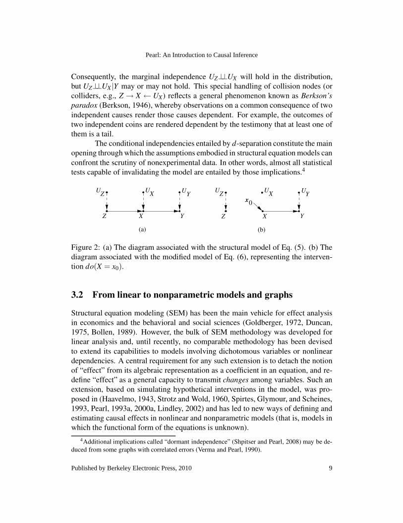
Consequently, the marginal independence UZ⊥⊥UX will hold in the distribution,

but UZ⊥⊥UX |Y may or may not hold. This special handling of collision nodes (or

colliders, e.g., Z → X ← UX) reflects a general phenomenon known as Berkson’s

paradox (Berkson, 1946), whereby observations on a common consequence of two

independent causes render those causes dependent. For example, the outcomes of

two independent coins are rendered dependent by the testimony that at least one of

them is a tail.

The conditional independencies entailed by d-separation constitute the main

opening through which the assumptions embodied in structural equation models can

confront the scrutiny of nonexperimental data. In other words, almost all statistical

tests capable of invalidating the model are entailed by those implications.4

Z X YZ X YU U U

Z X

0x

(b)

Y

U U U

(a)

X YZ

Figure 2: (a) The diagram associated with the structural model of Eq. (5). (b) The

diagram associated with the modified model of Eq. (6), representing the interven-

tion do(X = x0).

3.2 From linear to nonparametric models and graphs

Structural equation modeling (SEM) has been the main vehicle for effect analysis

in economics and the behavioral and social sciences (Goldberger, 1972, Duncan,

1975, Bollen, 1989). However, the bulk of SEM methodology was developed for

linear analysis and, until recently, no comparable methodology has been devised

to extend its capabilities to models involving dichotomous variables or nonlinear

dependencies. A central requirement for any such extension is to detach the notion

of “effect” from its algebraic representation as a coefficient in an equation, and re-

define “effect” as a general capacity to transmit changes among variables. Such an

extension, based on simulating hypothetical interventions in the model, was pro-

posed in (Haavelmo, 1943, Strotz and Wold, 1960, Spirtes, Glymour, and Scheines,

1993, Pearl, 1993a, 2000a, Lindley, 2002) and has led to new ways of defining and

estimating causal effects in nonlinear and nonparametric models (that is, models in

which the functional form of the equations is unknown).

4Additional implications called “dormant independence” (Shpitser and Pearl, 2008) may be de-

duced from some graphs with correlated errors (Verma and Pearl, 1990).

9



The central idea is to exploit the invariant characteristics of structural equa-

tions without committing to a specific functional form. For example, the non-

parametric interpretation of the diagram of Fig. 2(a) corresponds to a set of three

functions, each corresponding to one of the observed variables:

z = fZ(uZ)

x = fX (z,uX ) (5)

y = fY (x,uY )

where in this particular example UZ,UX and UY are assumed to be jointly inde-

pendent but, otherwise, arbitrarily distributed. Each of these functions represents a

causal process (or mechanism) that determines the value of the left variable (output)

from those on the right variables (inputs). The absence of a variable from the right

hand side of an equation encodes the assumption that Nature ignores that variable

in the process of determining the value of the output variable. For example, the

absence of variable Z from the arguments of fY conveys the empirical claim that

variations in Z will leave Y unchanged, as long as variables UY , and X remain con-

stant. A system of such functions are said to be structural if they are assumed to

be autonomous, that is, each function is invariant to possible changes in the form of

the other functions (Simon, 1953, Koopmans, 1953).

3.2.1 Representing interventions

This feature of invariance permits us to use structural equations as a basis for mod-

eling causal effects and counterfactuals. This is done through a mathematical oper-

ator called do(x) which simulates physical interventions by deleting certain func-

tions from the model, replacing them by a constant X = x, while keeping the rest of

the model unchanged. For example, to emulate an intervention do(x0) that holds X

constant (at X = x0) in model M of Fig. 2(a), we replace the equation for x in Eq.

(5) with x = x0, and obtain a new model, Mx0,

z = fZ(uZ)

x = x0 (6)

y = fY (x,uY )

the graphical description of which is shown in Fig. 2(b).

The joint distribution associated with the modified model, denoted

P(z,y|do(x0)) describes the post-intervention distribution of variables Y and Z (also

called “controlled” or “experimental” distribution), to be distinguished from the

pre-intervention distribution, P(x,y, z), associated with the original model of Eq.

10



(5). For example, if X represents a treatment variable, Y a response variable, and Z

some covariate that affects the amount of treatment received, then the distribution

P(z,y|do(x0)) gives the proportion of individuals that would attain response level

Y = y and covariate level Z = z under the hypothetical situation in which treatment

X = x0 is administered uniformly to the population.

In general, we can formally define the post-intervention distribution by the

equation:

PM(y|do(x))∆= PMx

(y) (7)

In words: In the framework of model M, the post-intervention distribution of out-

come Y is defined as the probability that model Mx assigns to each outcome level

Y = y.

From this distribution, one is able to assess treatment efficacy by comparing

aspects of this distribution at different levels of x0. A common measure of treatment

efficacy is the average difference

E(Y |do(x′0))−E(Y |do(x0)) (8)

where x′0

and x0 are two levels (or types) of treatment selected for comparison.

Another measure is the experimental Risk Ratio

E(Y |do(x′0))/E(Y |do(x0)). (9)

The variance Var(Y |do(x0)), or any other distributional parameter, may also enter

the comparison; all these measures can be obtained from the controlled distribu-

tion function P(Y = y|do(x)) = ∑z P(z,y|do(x)) which was called “causal effect” in

Pearl (2000a, 1995) (see footnote 2). The central question in the analysis of causal

effects is the question of identification: Can the controlled (post-intervention) dis-

tribution, P(Y = y|do(x)), be estimated from data governed by the pre-intervention

distribution, P(z,x,y)?The problem of identification has received considerable attention in econo-

metrics (Hurwicz, 1950, Marschak, 1950, Koopmans, 1953) and social science

(Duncan, 1975, Bollen, 1989), usually in linear parametric settings, where it re-

duces to asking whether some model parameter, β , has a unique solution in terms

of the parameters of P (the distribution of the observed variables). In the nonpara-

metric formulation, identification is more involved, since the notion of “has a unique

solution” does not directly apply to causal quantities such as Q(M) = P(y|do(x))which have no distinct parametric signature, and are defined procedurally by sim-

ulating an intervention in a causal model M (as in (6)). The following definition

overcomes these difficulties:

11



Definition 2 (Identifiability (Pearl, 2000a, p. 77)) A quantity Q(M) is identifiable,

given a set of assumptions A, if for any two models M1 and M2 that satisfy A, we

have

P(M1) = P(M2)⇒Q(M1) = Q(M2) (10)

In words, the details of M1 and M2 do not matter; what matters is that the

assumptions in A (e.g., those encoded in the diagram) would constrain the variabil-

ity of those details in such a way that equality of P’s would entail equality of Q’s.

When this happens, Q depends on P only, and should therefore be expressible in

terms of the parameters of P. The next subsections exemplify and operationalize

this notion.

3.2.2 Estimating the effect of interventions

To understand how hypothetical quantities such as P(y|do(x)) or E(Y |do(x0)) can

be estimated from actual data and a partially specified model let us begin with a

simple demonstration on the model of Fig. 2(a). We will see that, despite our igno-

rance of fX , fY , fZ and P(u), E(Y |do(x0)) is nevertheless identifiable and is given

by the conditional expectation E(Y |X = x0). We do this by deriving and comparing

the expressions for these two quantities, as defined by (5) and (6), respectively. The

mutilated model in Eq. (6) dictates:

E(Y |do(x0)) = E( fY (x0,uY )), (11)

whereas the pre-intervention model of Eq. (5) gives

E(Y |X = x0)) = E( fY (X ,uY )|X = x0)

= E( fY (x0,uY )|X = x0) (12)

= E( fY (x0,uY ))

which is identical to (11). Therefore,

E(Y |do(x0)) = E(Y |X = x0)) (13)

Using a similar derivation, though somewhat more involved, we can show that

P(y|do(x)) is identifiable and given by the conditional probability P(y|x).We see that the derivation of (13) was enabled by two assumptions; first, Y

is a function of X and UY only, and, second, UY is independent of {UZ,UX}, hence

of X . The latter assumption parallels the celebrated “orthogonality” condition in

linear models, Cov(X ,UY) = 0, which has been used routinely, often thoughtlessly,

to justify the estimation of structural coefficients by regression techniques.

12



Naturally, if we were to apply this derivation to the linear models of Fig.

1(a) or 1(b), we would get the expected dependence between Y and the intervention

do(x0):

E(Y |do(x0)) = E( fY (x0,uY ))

= E(βx0 +uY )

= βx0

(14)

This equality endows β with its causal meaning as “effect coefficient.” It is ex-

tremely important to keep in mind that in structural (as opposed to regressional)

models, β is not “interpreted” as an effect coefficient but is “proven” to be one by

the derivation above. β will retain this causal interpretation regardless of how X is

actually selected (through the function fX , Fig. 2(a)) and regardless of whether UX

and UY are correlated (as in Fig. 1(b)) or uncorrelated (as in Fig. 1(a)). Correlations

may only impede our ability to estimate β from nonexperimental data, but will not

change its definition as given in (14). Accordingly, and contrary to endless confu-

sions in the literature (see footnote 12) structural equations say absolutely nothing

about the conditional expectation E(Y |X = x). Such connection may exist under

special circumstances, e.g., if cov(X ,UY ) = 0, as in Eq. (13), but is otherwise irrel-

evant to the definition or interpretation of β as effect coefficient, or to the empirical

claims of Eq. (1).

The next subsection will circumvent these derivations altogether by reduc-

ing the identification problem to a graphical procedure. Indeed, since graphs encode

all the information that non-parametric structural equations represent, they should

permit us to solve the identification problem without resorting to algebraic analysis.

3.2.3 Causal effects from data and graphs

Causal analysis in graphical models begins with the realization that all causal ef-

fects are identifiable whenever the model is Markovian, that is, the graph is acyclic

(i.e., containing no directed cycles) and all the error terms are jointly independent.

Non-Markovian models, such as those involving correlated errors (resulting from

unmeasured confounders), permit identification only under certain conditions, and

these conditions too can be determined from the graph structure (Section 3.3). The

key to these results rests with the following basic theorem.

Theorem 1 (The Causal Markov Condition) Any distribution generated by a Marko-

vian model M can be factorized as:

P(v1,v2, . . .,vn) = ∏i

P(vi|pai) (15)

13



where V1,V2, . . .,Vn are the endogenous variables in M, and pai are (values of) the

endogenous “parents” of Vi in the causal diagram associated with M.

For example, the distribution associated with the model in Fig. 2(a) can be

factorized as

P(z,y,x) = P(z)P(x|z)P(y|x) (16)

since X is the (endogenous) parent of Y,Z is the parent of X , and Z has no parents.

Corollary 1 (Truncated factorization) For any Markovian model, the distribution

generated by an intervention do(X = x0) on a set X of endogenous variables is

given by the truncated factorization

P(v1,v2, . . .,vk|do(x0)) = ∏i|Vi 6∈X

P(vi|pai) |x=x0(17)

where P(vi|pai) are the pre-intervention conditional probabilities.5

Corollary 1 instructs us to remove from the product of Eq. (15) those fac-

tors that quantify how the intervened variables (members of set X) are influenced

by their pre-intervention parents. This removal follows from the fact that the post-

intervention model is Markovian as well, hence, following Theorem 1, it must

generate a distribution that is factorized according to the modified graph, yielding

the truncated product of Corollary 1. In our example of Fig. 2(b), the distribution

P(z,y|do(x0)) associated with the modified model is given by

P(z,y|do(x0)) = P(z)P(y|x0)

where P(z) and P(y|x0) are identical to those associated with the pre-intervention

distribution of Eq. (16). As expected, the distribution of Z is not affected by the

intervention, since

P(z|do(x0)) = ∑y

P(z,y|do(x0)) = ∑y

P(z)P(y|x0) = P(z)

while that of Y is sensitive to x0, and is given by

P(y|do(x0)) = ∑z

P(z,y|do(x0)) = ∑z

P(z)P(y|x0) = P(y|x0)

This example demonstrates how the (causal) assumptions embedded in the model

M permit us to predict the post-intervention distribution from the pre-intervention

5A simple proof of the Causal Markov Theorem is given in Pearl (2000a, p. 30). This theorem

was first presented in Pearl and Verma (1991), but it is implicit in the works of Kiiveri, Speed, and

Carlin (1984) and others. Corollary 1 was named “Manipulation Theorem” in Spirtes et al. (1993),

and is also implicit in Robins’ (1987) G-computation formula. See Lauritzen (2001).

14



distribution, which further permits us to estimate the causal effect of X on Y from

nonexperimental data, since P(y|x0) is estimable from such data. Note that we have

made no assumption whatsoever on the form of the equations or the distribution of

the error terms; it is the structure of the graph alone (specifically, the identity of X’s

parents) that permits the derivation to go through.

The truncated factorization formula enables us to derive causal quantities

directly, without dealing with equations or equation modification as in Eqs. (11)–

(13). Consider, for example, the model shown in Fig. 3, in which the error variables

Z1

Z3

Z2

Y

X

Figure 3: Markovian model illustrating the derivation of the causal effect of X on

Y , Eq. (20). Error terms are not shown explicitly.

are kept implicit. Instead of writing down the corresponding five nonparametric

equations, we can write the joint distribution directly as

P(x, z1, z2, z3,y) = P(z1)P(z2)P(z3|z1, z2)P(x|z1, z3)P(y|z2 , z3,x) (18)

where each marginal or conditional probability on the right hand side is directly

estimable from the data. Now suppose we intervene and set variable X to x0. The

post-intervention distribution can readily be written (using the truncated factoriza-

tion formula (17)) as

P(z1, z2, z3,y|do(x0)) = P(z1)P(z2)P(z3|z1, z2)P(y|z2, z3,x0) (19)

and the causal effect of X on Y can be obtained immediately by marginalizing over

the Z variables, giving

P(y|do(x0)) = ∑z1,z2,z3

P(z1)P(z2)P(z3|z1, z2)P(y|z2, z3,x0) (20)

Note that this formula corresponds precisely to what is commonly called “adjusting

for Z1,Z2 and Z3” and, moreover, we can write down this formula by inspection,

without thinking on whether Z1,Z2 and Z3 are confounders, whether they lie on

the causal pathways, and so on. Though such questions can be answered explicitly

15



from the topology of the graph, they are dealt with automatically when we write

down the truncated factorization formula and marginalize.

Note also that the truncated factorization formula is not restricted to inter-

ventions on a single variable; it is applicable to simultaneous or sequential inter-

ventions such as those invoked in the analysis of time varying treatment with time

varying confounders (Robins, 1986, Arjas and Parner, 2004). For example, if X

and Z2 are both treatment variables, and Z1 and Z3 are measured covariates, then

the post-intervention distribution would be

P(z1, z3,y|do(x),do(z2)) = P(z1)P(z3|z1, z2)P(y|z2, z3,x) (21)

and the causal effect of the treatment sequence do(X = x),do(Z2 = z2)6 would be

P(y|do(x),do(z2)) = ∑z1,z3

P(z1)P(z3|z1, z2)P(y|z2 , z3,x) (22)

This expression coincides with Robins’ (1987) G-computation formula,

which was derived from a more complicated set of (counterfactual) assumptions.

As noted by Robins, the formula dictates an adjustment for covariates (e.g., Z3) that

might be affected by previous treatments (e.g., Z2).

3.3 Coping with unmeasured confounders

Things are more complicated when we face unmeasured confounders. For example,

it is not immediately clear whether the formula in Eq. (20) can be estimated if any of

Z1,Z2 and Z3 is not measured. A few but challenging algebraic steps would reveal

that one can perform the summation over Z2 to obtain

P(y|do(x0)) = ∑z1,z3

P(z1)P(z3|z1)P(y|z1 , z3,x0) (23)

which means that we need only adjust for Z1 and Z3 without ever measuring Z2. In

general, it can be shown (Pearl, 2000a, p. 73) that, whenever the graph is Markovian

the post-interventional distribution P(Y = y|do(X = x)) is given by the following

expression:

P(Y = y|do(X = x)) = ∑t

P(y|t,x)P(t) (24)

where T is the set of direct causes of X (also called “parents”) in the graph. This

allows us to write (23) directly from the graph, thus skipping the algebra that led to

(23). It further implies that, no matter how complicated the model, the parents of X

are the only variables that need to be measured to estimate the causal effects of X .

6For clarity, we drop the (superfluous) subscript 0 from x0 and z20.

16



It is not immediately clear however whether other sets of variables beside

X’s parents suffice for estimating the effect of X , whether some algebraic manipu-

lation can further reduce Eq. (23), or that measurement of Z3 (unlike Z1, or Z2) is

necessary in any estimation of P(y|do(x0)). Such considerations become transpar-

ent from a graphical criterion to be discussed next.

3.3.1 Covariate selection – the back-door criterion

Consider an observational study where we wish to find the effect of X on Y , for

example, treatment on response, and assume that the factors deemed relevant to

the problem are structured as in Fig. 4; some are affecting the response, some are

Z1

Z3

Z2

Y

X

W

W

W

1

2

3

Figure 4: Markovian model illustrating the back-door criterion. Error terms are not

shown explicitly.

affecting the treatment and some are affecting both treatment and response. Some

of these factors may be unmeasurable, such as genetic trait or life style, others

are measurable, such as gender, age, and salary level. Our problem is to select a

subset of these factors for measurement and adjustment, namely, that if we compare

treated vs. untreated subjects having the same values of the selected factors, we

get the correct treatment effect in that subpopulation of subjects. Such a set of

factors is called a “sufficient set” or “admissible set” for adjustment. The problem

of defining an admissible set, let alone finding one, has baffled epidemiologists and

social scientists for decades (see (Greenland et al., 1999, Pearl, 1998) for review).

The following criterion, named “back-door” in (Pearl, 1993a), settles this

problem by providing a graphical method of selecting admissible sets of factors for

adjustment.

Definition 3 (Admissible sets – the back-door criterion) A set S is admissible (or

“sufficient”) for adjustment if two conditions hold:

1. No element of S is a descendant of X

17



2. The elements of S “block” all “back-door” paths from X to Y, namely all

paths that end with an arrow pointing to X.

In this criterion, “blocking” is interpreted as in Definition 1. For example, the set

S = {Z3} blocks the path X ←W1 ← Z1 → Z3 → Y , because the arrow-emitting

node Z3 is in S. However, the set S = {Z3} does not block the path X ←W1 ←Z1→ Z3← Z2→W2→ Y , because none of the arrow-emitting nodes, Z1 and Z2, is

in S, and the collision node Z3 is not outside S.

Based on this criterion we see, for example, that the sets {Z 1,Z 2,Z 3},{Z 1,Z 3},{W1,Z3}, and {W2,Z3}, each is sufficient for adjustment, because each blocks all

back-door paths between X and Y . The set {Z3}, however, is not sufficient for ad-

justment because, as explained above, it does not block the path X ←W1← Z1→Z3← Z2→W2→ Y .

The intuition behind the back-door criterion is as follows. The back-door

paths in the diagram carry spurious associations from X to Y , while the paths di-

rected along the arrows from X to Y carry causative associations. Blocking the

former paths (by conditioning on S) ensures that the measured association between

X and Y is purely causative, namely, it correctly represents the target quantity: the

causal effect of X on Y . The reason for excluding descendants of X (e.g., W3 or any

of its descendants) is given in (Pearl, 2009b, pp. 338–41).

Formally, the implication of finding an admissible set S is that, stratifying

on S is guaranteed to remove all confounding bias relative the causal effect of X on

Y . In other words, the risk difference in each stratum of S gives the correct causal

effect in that stratum. In the binary case, for example, the risk difference in stratum

s of S is given by

P(Y = 1|X = 1,S = s)−P(Y = 1|X = 0,S = s)

while the causal effect (of X on Y ) at that stratum is given by

P(Y = 1|do(X = 1),S = s)−P(Y = 1|do(X = 0),S = s).

These two expressions are guaranteed to be equal whenever S is a sufficient set, such

as {Z1,Z3} or {Z2,Z3} in Fig. 4. Likewise, the average stratified risk difference,

taken over all strata,

∑s

[P(Y = 1|X = 1,S = s)−P(Y = 1|X = 0,S = s)]P(S = s),

gives the correct causal effect of X on Y in the entire population

P(Y = 1|do(X = 1))−P(Y = 1|do(X = 0)).

18



In general, for multi-valued variables X and Y , finding a sufficient set S

permits us to write

P(Y = y|do(X = x),S = s) = P(Y = y|X = x,S = s)

and

P(Y = y|do(X = x)) = ∑s

P(Y = y|X = x,S = s)P(S = s) (25)

Since all factors on the right hand side of the equation are estimable (e.g., by regres-

sion) from the pre-interventional data, the causal effect can likewise be estimated

from such data without bias.

An equivalent expression for the causal effect (25) can be obtained by mul-

tiplying and dividing by the conditional probability P(X = x|S = s), giving

P(Y = y|do(X = x)) = ∑s

P(Y = y,X = x,S = s)

P(X = x|S = s)(26)

from which the name “Inverse Probability Weighting” has evolved (Pearl, 2000a,

pp. 73, 95).

Interestingly, it can be shown that any irreducible sufficient set, S, taken as

a unit, satisfies the associational criterion that epidemiologists have been using to

define “confounders”. In other words, S must be associated with X and, simultane-

ously, associated with Y , given X . This need not hold for any specific members of

S. For example, the variable Z3 in Fig. 4, though it is a member of every sufficient

set and hence a confounder, can be unassociated with both Y and X (Pearl, 2000a,

p. 195). Conversely, a pre-treatment variable Z that is associated with both Y and X

may need to be excluded from entering a sufficient set.

The back-door criterion allows us to write Eq. (25) directly, by selecting a

sufficient set S directly from the diagram, without manipulating the truncated factor-

ization formula. The selection criterion can be applied systematically to diagrams

of any size and shape, thus freeing analysts from judging whether “X is condition-

ally ignorable given S,” a formidable mental task required in the potential-response

framework (Rosenbaum and Rubin, 1983). The criterion also enables the analyst to

search for an optimal set of covariate—namely, a set S that minimizes measurement

cost or sampling variability (Tian, Paz, and Pearl, 1998).

All in all, one can safely state that, armed with the back-door criterion,

causality has removed “confounding” from its store of enigmatic and controversial

concepts.

19



3.3.2 Confounding equivalence – a graphical test

Another problem that has been given graphical solution recently is that of deter-

mining whether adjustment for two sets of covariates would result in the same con-

founding bias (Pearl and Paz, 2009). The reasons for posing this question are sev-

eral. First, an investigator may wish to assess, prior to taking any measurement,

whether two candidate sets of covariates, differing substantially in dimensionality,

measurement error, cost, or sample variability are equally valuable in their bias-

reduction potential. Second, assuming that the structure of the underlying DAG is

only partially known, one may wish to test, using adjustment, which of two hypoth-

esized structures is compatible with the data. Structures that predict equal response

to adjustment for two sets of variables must be rejected if, after adjustment, such

equality is not found in the data.

Definition 4 ((c-equivalence)) Define two sets, T and Z of covariates as

c-equivalent, (c connotes “confounding”) if the following equality holds:

∑t

P(y|x, t)P(t) = ∑z

P(y|x, z)P(z) ∀x,y (27)

Definition 5 ((Markov boundary)) For any set of variables S in a DAG G, the

Markov boundary Sm of S is the minimal subset of S that d-separates X from all

other members of S.

In Fig. 4, for example, the Markov boundary of S = {W1,Z1,Z2,Z3} is Sm ={W1,Z3}.

Theorem 2 (Pearl and Paz, 2009)

Let Z and T be two sets of variables in G, containing no descendant of X. A

necessary and sufficient conditions for Z and T to be c-equivalent is that at least

one of the following conditions holds:

1. Zm = Tm, (i.e., the Markov boundary of Z coincides with that of T )

2. Z and T are admissible (i.e., satisfy the back-door condition)

For example, the sets T = {W1,Z3} and Z = {Z3,W2} in Fig. 4 are

c-equivalent, because each blocks all back-door paths from X to Y . Similarly,

the non-admissible sets T = {Z2} and Z = {W2,Z2} are c-equivalent, since their

Markov boundaries are the same (Tm = Zm = {Z2}). In contrast, the sets {W1} and

20



{Z1}, although they block the same set of paths in the graph, are not c-equivalent;

they fail both conditions of Theorem 2.

Tests for c-equivalence (27) are fairly easy to perform, and they can also

be assisted by propensity scores methods. The information that such tests provide

can be as powerful as conditional independence tests. The statistical ramification

of such tests are explicated in (Pearl and Paz, 2009).

3.3.3 General control of confounding

Adjusting for covariates is only one of many methods that permits us to estimate

causal effects in nonexperimental studies. Pearl (1995) has presented examples in

which there exists no set of variables that is sufficient for adjustment and where the

causal effect can nevertheless be estimated consistently. The estimation, in such

cases, employs multi-stage adjustments. For example, if W3 is the only observed

covariate in the model of Fig. 4, then there exists no sufficient set for adjustment

(because no set of observed covariates can block the paths from X to Y through

Z3), yet P(y|do(x)) can be estimated in two steps; first we estimate P(w3|do(x)) =P(w3|x) (by virtue of the fact that there exists no unblocked back-door path from X

to W3), second we estimate P(y|do(w3)) (since X constitutes a sufficient set for the

effect of W3 on Y ) and, finally, we combine the two effects together and obtain

P(y|do(x)) = ∑w3

P(w3|do(x))P(y|do(w3)) (28)

In this example, the variable W3 acts as a “mediating instrumental variable” (Pearl,

1993b, Chalak and White, 2006).

The analysis used in the derivation and validation of such results invokes

mathematical rules of transforming causal quantities, represented by expressions

such as P(Y = y|do(x)), into do-free expressions derivable from P(z,x,y), since

only do-free expressions are estimable from non-experimental data. When such a

transformation is feasible, we are ensured that the causal quantity is identifiable.

Applications of this calculus to problems involving multiple interventions

(e.g., time varying treatments), conditional policies, and surrogate experiments

were developed in Pearl and Robins (1995), Kuroki and Miyakawa (1999), and

Pearl (2000a, Chapters 3–4).

A more recent analysis (Tian and Pearl, 2002) shows that the key to iden-

tifiability lies not in blocking paths between X and Y but, rather, in blocking paths

between X and its immediate successors on the pathways to Y . All existing criteria

for identification are special cases of the one defined in the following theorem:

21



Theorem 3 (Tian and Pearl, 2002) A sufficient condition for identifying the causal

effect P(y|do(x)) is that every path between X and any of its children traces at least

one arrow emanating from a measured variable.7

For example, if W3 is the only observed covariate in the model of Fig. 4, P(y|do(x))can be estimated since every path from X to W3 (the only child of X) traces either

the arrow X→W3, or the arrow W3→Y , both emanating from a measured variable

(W3).Shpitser and Pearl (2006) have further extended this theorem by (1) pre-

senting a necessary and sufficient condition for identification, and (2) extending the

condition from causal effects to any counterfactual expression. The correspond-

ing unbiased estimands for these causal quantities are readable directly from the

diagram.

Graph-based methods for effect identification under measurement errors are

discussed in (Pearl, 2009f, Hernan and Cole, 2009, Cai and Kuroki, 2008).

3.3.4 From identification to estimation

The mathematical derivation of causal effect estimands, like Eqs. (25) and (28) is

merely a first step toward computing quantitative estimates of those effects from

finite samples, using the rich traditions of statistical estimation and machine learn-

ing Bayesian as well as non-Bayesian. Although the estimands derived in (25)

and (28) are non-parametric, this does not mean that one should refrain from us-

ing parametric forms in the estimation phase of the study. Parameterization is

in fact necessary when the dimensionality of a problem is high. For example, if

the assumptions of Gaussian, zero-mean disturbances and additive interactions are

deemed reasonable, then the estimand given in (28) can be converted to the prod-

uct E(Y |do(x)) = rW3XrYW3·X x, where rY Z·X is the (standardized) coefficient of Z in

the regression of Y on Z and X . More sophisticated estimation techniques are the

“marginal structural models” of (Robins, 1999), and the “propensity score” method

of (Rosenbaum and Rubin, 1983) which were found to be particularly useful when

dimensionality is high and data are sparse (see Pearl (2009b, pp. 348–52)).

It should be emphasized, however, that contrary to conventional wisdom

(e.g., (Rubin, 2007, 2009)), propensity score methods are merely efficient estima-

tors of the right hand side of (25); they entail the same asymptotic bias, and cannot

be expected to reduce bias in case the set S does not satisfy the back-door crite-

rion (Pearl, 2000a, 2009c,d). Consequently, the prevailing practice of conditioning

7Before applying this criterion, one may delete from the causal graph all nodes that are not

ancestors of Y .

22



on as many pre-treatment measurements as possible should be approached with

great caution; some covariates (e.g., Z3 in Fig. 3) may actually increase bias if in-

cluded in the analysis (see footnote 16). Using simulation and parametric analysis,

Heckman and Navarro-Lozano (2004) and Wooldridge (2009) indeed confirmed the

bias-raising potential of certain covariates in propensity-score methods. The graph-

ical tools presented in this section unveil the character of these covariates and show

precisely what covariates should, and should not be included in the conditioning set

for propensity-score matching (see also (Pearl and Paz, 2009, Pearl, 2009e)).

3.4 Counterfactual analysis in structural models

Not all questions of causal character can be encoded in P(y|do(x)) type expressions,

thus implying that not all causal questions can be answered from experimental stud-

ies. For example, questions of attribution (e.g., what fraction of death cases are due

to specific exposure?) or of susceptibility (what fraction of the healthy unexposed

population would have gotten the disease had they been exposed?) cannot be an-

swered from experimental studies, and naturally, this kind of questions cannot be

expressed in P(y|do(x)) notation.8 To answer such questions, a probabilistic anal-

ysis of counterfactuals is required, one dedicated to the relation “Y would be y had

X been x in situation U = u,” denoted Yx(u) = y. Remarkably, unknown to most

economists and philosophers, structural equation models provide the formal inter-

pretation and symbolic machinery for analyzing such counterfactual relationships.9

The key idea is to interpret the phrase “had X been x” as an instruction to

make a minimal modification in the current model, which may have assigned X a

different value, say X = x′, so as to ensure the specified condition X = x. Such a

minimal modification amounts to replacing the equation for X by a constant x, as

we have done in Eq. (6). This replacement permits the constant x to differ from

the actual value of X (namely fX (z,uX)) without rendering the system of equations

inconsistent, thus yielding a formal interpretation of counterfactuals in multi-stage

8The reason for this fundamental limitation is that no death case can be tested twice, with and

without treatment. For example, if we measure equal proportions of deaths in the treatment and

control groups, we cannot tell how many death cases are actually attributable to the treatment itself;

it is quite possible that many of those who died under treatment would be alive if untreated and,

simultaneously, many of those who survived with treatment would have died if not treated.9Connections between structural equations and a restricted class of counterfactuals were first rec-

ognized by Simon and Rescher (1966). These were later generalized by Balke and Pearl (1995), us-

ing surgeries (Eq. (29)), thus permitting endogenous variables to serve as counterfactual antecedents.

The term “surgery definition” was used in Pearl (2000a, Epilogue) and criticized by Cartwright

(2007) and Heckman (2005), (see Pearl (2009b, pp. 362–3, 374–9 for rebuttals)).

23



models, where the dependent variable in one equation may be an independent vari-

able in another.

Definition 6 (Unit-level Counterfactuals – “surgical” definition, Pearl (2000a, p. 98))

Let M be a structural model and Mx a modified version of M, with the equation(s)

of X replaced by X = x. Denote the solution for Y in the equations of Mx by the

symbol YMx(u). The counterfactual Yx(u) (Read: “The value of Y in unit u, had X

been x”) is given by:

Yx(u)∆= YMx

(u). (29)

In words: The counterfactual Yx(u) in model M is defined as the solution for Y in

the “surgically modified” submodel Mx.

We see that the unit-level counterfactual Yx(u), which in the Neyman-Rubin

approach is treated as a primitive, undefined quantity, is actually a derived quantity

in the structural framework. The fact that we equate the experimental unit u with

a vector of background conditions, U = u, in M, reflects the understanding that the

name of a unit or its identity do not matter; it is only the vector U = u of attributes

characterizing a unit which determines its behavior or response. As we go from one

unit to another, the laws of nature, as they are reflected in the functions fX , fY , etc.

remain invariant; only the attributes U = u vary from individual to individual.10

To illustrate, consider the solution of Y in the modified model Mx0of Eq.

(6), which Definition 6 endows with the symbol Yx0(uX ,uY ,uZ). This entity has

a clear counterfactual interpretation, for it stands for the way an individual with

characteristics (uX ,uY ,uZ) would respond, had the treatment been x0, rather than

the treatment x = fX (z,uX) actually received by that individual. In our example,

since Y does not depend on uX and uZ , we can write:

Yx0(u) = Yx0

(uY ,uX ,uZ) = fY (x0,uY ). (30)

In a similar fashion, we can derive

Yz0(u) = fY ( fX (z0,uX),uY ),

10The distinction between general, or population-level causes (e.g., “Drinking hemlock causes

death”) and singular or unit-level causes (e.g., “Socrates’ drinking hemlock caused his death”),

which many philosophers have regarded as irreconcilable (Eells, 1991), introduces no tension at all

in the structural theory. The two types of sentences differ merely in the level of situation-specific

information that is brought to bear on a problem, that is, in the specificity of the evidence e that

enters the quantity P(Yx = y|e). When e includes all factors u, we have a deterministic, unit-level

causation on our hand; when e contains only a few known attributes (e.g., age, income, occupation

etc.) while others are assigned probabilities, a population-level analysis ensues.

24



Xz0,y0(u) = fX (z0,uX),

and so on. These examples reveal the counterfactual reading of each individual

structural equation in the model of Eq. (5). The equation x = fX (z,uX), for example,

advertises the empirical claim that, regardless of the values taken by other variables

in the system, had Z been z0, X would take on no other value but x = fX (z0,uX).Clearly, the distribution P(uY ,uX ,uZ) induces a well defined probability on

the counterfactual event Yx0= y, as well as on joint counterfactual events, such as

‘Yx0= y AND Yx1

= y′,’ which are, in principle, unobservable if x0 6= x1. Thus, to

answer attributional questions, such as whether Y would be y1 if X were x1, given

that in fact Y is y0 and X is x0, we need to compute the conditional probability

P(Yx1= y1|Y = y0,X = x0) which is well defined once we know the forms of the

structural equations and the distribution of the exogenous variables in the model.

For example, assuming linear equations (as in Fig. 1),

x = uX y = βx+uX ,

the conditioning events Y = y0 and X = x0 yield UX = x0 and UY = y0− βx0, and

we can conclude that, with probability one, Yx1must take on the value: Yx1

= βx1 +UY = β(x1− x0)+ y0. In other words, if X were x1 instead of x0, Y would increase

by β times the difference (x1− x0). In nonlinear systems, the result would also

depend on the distribution of {UX ,UY} and, for that reason, attributional queries

are generally not identifiable in nonparametric models (see Section 6.3 and 2000a,

Chapter 9).

In general, if x and x′ are incompatible then Yx and Yx′ cannot be measured

simultaneously, and it may seem meaningless to attribute probability to the joint

statement “Y would be y if X = x and Y would be y′ if X = x′.”11 Such concerns

have been a source of objections to treating counterfactuals as jointly distributed

random variables (Dawid, 2000). The definition of Yx and Yx′ in terms of two distinct

submodels neutralizes these objections (Pearl, 2000b), since the contradictory joint

statement is mapped into an ordinary event, one where the background variables

satisfy both statements simultaneously, each in its own distinct submodel; such

events have well defined probabilities.

The surgical definition of counterfactuals given by (29), provides the con-

ceptual and formal basis for the Neyman-Rubin potential-outcome framework, an

approach to causation that takes a controlled randomized trial (CRT) as its rul-

ing paradigm, assuming that nothing is known to the experimenter about the sci-

ence behind the data. This “black-box” approach, which has thus far been denied

the benefits of graphical or structural analyses, was developed by statisticians who

11For example, “The probability is 80% that Joe belongs to the class of patients who will be cured

if they take the drug and die otherwise.”

25



found it difficult to cross the two mental barriers discussed in Section 2.2. Section

5 establishes the precise relationship between the structural and potential-outcome

paradigms, and outlines how the latter can benefit from the richer representational

power of the former.

4 Methodological Principles of Causal Inference

The structural theory described in the previous sections dictates a principled method-

ology that eliminates much of the confusion concerning the interpretations of study

results as well as the ethical dilemmas that this confusion tends to spawn. The

methodology dictates that every investigation involving causal relationships (and

this entails the vast majority of empirical studies in the health, social, and behav-

ioral sciences) should be structured along the following four-step process:

1. Define: Express the target quantity Q as a function Q(M) that can be com-

puted from any model M.

2. Assume: Formulate causal assumptions using ordinary scientific language

and represent their structural part in graphical form.

3. Identify: Determine if the target quantity is identifiable (i.e., expressible in

terms of estimable parameters).

4. Estimate: Estimate the target quantity if it is identifiable, or approximate it,

if it is not. Test the statistical implications of the model, if any, and modify

the model when failure occurs.

4.1 Defining the target quantity

The definitional phase is the most neglected step in current practice of quantitative

analysis. The structural modeling approach insists on defining the target quantity,

be it “causal effect,” “mediated effect,” “effect on the treated,” or “probability of

causation” before specifying any aspect of the model, without making functional or

distributional assumptions and prior to choosing a method of estimation.

The investigator should view this definition as an algorithm that receives a

model M as an input and delivers the desired quantity Q(M) as the output. Surely,

such algorithm should not be tailored to any aspect of the input M; it should be gen-

eral, and ready to accommodate any conceivable model M whatsoever. Moreover,

the investigator should imagine that the input M is a completely specified model,

with all the functions fX , fY , . . . and all the U variables (or their associated probabil-

ities) given precisely. This is the hardest step for statistically trained investigators

to make; knowing in advance that such model details will never be estimable from

26



the data, the definition of Q(M) appears like a futile exercise in fantasy land – it is

not.

For example, the formal definition of the causal effect P(y|do(x)), as given

in Eq. (7), is universally applicable to all models, parametric as well as nonpara-

metric, through the formation of a submodel Mx. By defining causal effect procedu-

rally, thus divorcing it from its traditional parametric representation, the structural

theory avoids the many pitfalls and confusions that have plagued the interpretation

of structural and regressional parameters for the past half century.12

4.2 Explicating causal assumptions

This is the second most neglected step in causal analysis. In the past, the diffi-

culty has been the lack of a language suitable for articulating causal assumptions

which, aside from impeding investigators from explicating assumptions, also inhib-

ited them from giving causal interpretations to their findings.

Structural equation models, in their counterfactual reading, have removed

this lingering difficulty by providing the needed language for causal analysis. Fig-

ures 3 and 4 illustrate the graphical component of this language, where assump-

tions are conveyed through the missing arrows in the diagram. If numerical or

functional knowledge is available, for example, linearity or monotonicity of the

functions fX , fY , . . ., those are stated separately, and applied in the identification

and estimation phases of the study. Today we understand that the longevity and

natural appeal of structural equations stem from the fact that they permit investiga-

tors to communicate causal assumptions formally and in the very same vocabulary

in which scientific knowledge is stored.

Unfortunately, however, this understanding is not shared by all causal ana-

lysts; some analysts vehemently oppose the re-emergence of structure-based causa-

tion and insist, instead, on articulating causal assumptions exclusively in the unnat-

ural (though formally equivalent) language of “potential outcomes,” “ignorability,”

“missing data,” “treatment assignment,” and other metaphors borrowed from clini-

cal trials. This modern assault on structural models is perhaps more dangerous than

the regressional invasion that distorted the causal readings of these models in the

12Note that β in Eq. (1), the incremental causal effect of X on Y , is defined procedurally by

β∆= E(Y |do(x0 +1))−E(Y |do(x0)) =

∂

∂ xE(Y |do(x)) =

∂

∂ xE(Yx).

Naturally, all attempts to give β statistical interpretation have ended in frustrations (Holland, 1988,

Whittaker, 1990, Wermuth, 1992, Wermuth and Cox, 1993), some persisting well into the 21st cen-

tury (Sobel, 2008).

27



late 1970s (Richard, 1980). While sanctioning causal inference in one idiosyncratic

style of analysis, the modern assault denies validity to any other style, including

structural equations, thus discouraging investigators from subjecting models to the

scrutiny of scientific knowledge.

This exclusivist attitude is manifested in passages such as: “The crucial

idea is to set up the causal inference problem as one of missing data” or “If a prob-

lem of causal inference cannot be formulated in this manner (as the comparison of

potential outcomes under different treatment assignments), it is not a problem of

inference for causal effects, and the use of “causal” should be avoided,” or, even

more bluntly, “the underlying assumptions needed to justify any causal conclusions

should be carefully and explicitly argued, not in terms of technical properties like

“uncorrelated error terms,” but in terms of real world properties, such as how the

units received the different treatments” (Wilkinson, the Task Force on Statistical

Inference, and APA Board of Scientific Affairs, 1999).

The methodology expounded in this paper testifies against such restric-

tions. It demonstrates the viability and scientific soundness of the traditional struc-

tural equations paradigm, which stands diametrically opposed to the “missing data”

paradigm. It renders the vocabulary of “treatment assignment” stifling and irrele-

vant (e.g., there is no “treatment assignment” in sex discrimination cases). Most

importantly, it strongly prefers the use of “uncorrelated error terms,” (or “omitted

factors”) over its “strong ignorability” alternative, as the proper way of articulating

causal assumptions. Even the most devout advocates of the “strong ignorability”

language use “omitted factors” when the need arises to defend assumptions (e.g.,

(Sobel, 2008))

4.3 Identification, estimation, and approximation

Having unburden itself from parametric representations, the identification process

in the structural framework proceeds either in the space of assumptions (i.e., the

diagram) or in the space of mathematical expressions, after translating the graph-

ical assumptions into a counterfactual language, as demonstrated in Section 5.3.

Graphical criteria such as those of Definition 3 and Theorem 3 permit the identifi-

cation of causal effects to be decided entirely within the graphical domain, where it

can benefit from the guidance of scientific understanding. Identification of counter-

factual queries, on the other hand, often require a symbiosis of both algebraic and

graphical techniques. The nonparametric nature of the identification task (Defini-

tion 1) makes it clear that contrary to traditional folklore in linear analysis, it is not

the model that need be identified but the query Q – the target of investigation. It

also provides a simple way of proving non-identifiability: the construction of two

28



parameterization of M, agreeing in P and disagreeing in Q, is sufficient to rule out

identifiability.

When Q is identifiable, the structural framework also delivers an algebraic

expression for the estimand EST (Q) of the target quantity Q, examples of which

are given in Eqs. (24) and (25), and estimation techniques are then unleashed as

discussed in Section 3.3.4. An integral part of this estimation phase is a test for

the testable implications, if any, of those assumptions in M that render Q identifi-

able – there is no point in estimating EST (Q) if the data proves those assumptions

false and EST (Q) turns out to be a misrepresentation of Q. Investigators should

be reminded, however, that only a fraction, called “kernel,” of the assumptions em-

bodied in M are needed for identifying Q (Pearl, 2004), the rest may be violated

in the data with no effect on Q. In Fig. 2, for example, the assumption {UZ⊥⊥UX}is not necessary for identifying Q = P(y|do(x)); the kernel {UY⊥⊥UZ,UY⊥⊥UX}(together with the missing arrows) is sufficient. Therefore, the testable implication

of this kernel, Z⊥⊥Y |X , is all we need to test when our target quantity is Q; the

assumption {UZ⊥⊥UX} need not concern us.

More importantly, investigators must keep in mind that only a tiny fraction

of any kernel lends itself to statistical tests, the bulk of it must remain untestable,

at the mercy of scientific judgment. In Fig. 2, for example, the assumption set

{UX⊥⊥UZ,UY⊥⊥UX} constitutes a sufficient kernel for Q = P(y|do(x)) (see Eq.

(28)) yet it has no testable implications whatsoever. The prevailing practice of

submitting an entire structural equation model to a “goodness of fit” test (Bollen,

1989) in support of causal claims is at odd with the logic of SCM (see (Pearl,

2000a, pp. 144–5)). Alternative causal models usually exist that make contradictory

claims and, yet, possess identical statistical implications. Statistical test can be

used for rejecting certain kernels, in the rare cases where such kernels have testable

implications, but the lion’s share of supporting causal claims falls on the shoulders

of untested causal assumptions.

When conditions for identification are not met, the best one can do is derive

bounds for the quantities of interest—namely, a range of possible values of Q that

represents our ignorance about the details of the data-generating process M and that

cannot be improved with increasing sample size. A classical example of non iden-

tifiable model that has been approximated by bounds, is the problem of estimating

causal effect in experimental studies marred by non compliance, the structure of

which is given in Fig. 5.

Our task in this example is to find the highest and lowest values of Q

Q∆= P(Y = y|do(x)) = ∑

uX

P(Y = y|X = x,UX = uX)P(UX = uX) (31)

subject to the equality constraints imposed by the observed probabilities P(x,y, |z),

29



X YZ U UU

YZ X

Figure 5: Causal diagram representing the assignment (Z), treatment (X), and out-

come (Y ) in a clinical trial with imperfect compliance.

where the maximization ranges over all possible functions P(uY ,uX), P(y|x,uX )and P(x|z,uY ) that satisfy those constraints.

Realizing that units in this example fall into 16 equivalence classes, each

representing a binary function X = f (z) paired with a binary function y = g(x),Balke and Pearl (1997) were able to derive closed-form solutions for these bounds.13

They showed that, in certain cases, the derived bounds can yield significant infor-

mation on the treatment efficacy. Chickering and Pearl (1997) further used Bayesian

techniques (with Gibbs sampling) to investigate the sharpness of these bounds as

a function of sample size. Kaufman, Kaufman, and MacLenose (2009) used this

technique to bound direct and indirect effects (see Section 6.1).

5 The Potential Outcome Framework

This section compares the structural theory presented in Sections 1–3 to the potential-

outcome framework, usually associated with the names of Neyman (1923) and Ru-

bin (1974), which takes the randomized experiment as its ruling paradigm and has

appealed therefore to researchers who do not find that paradigm overly constrain-

ing. This framework is not a contender for a comprehensive theory of causation

for it is subsumed by the structural theory and excludes ordinary cause-effect rela-

tionships from its assumption vocabulary. We here explicate the logical foundation

of the Neyman-Rubin framework, its formal subsumption by the structural causal

model, and how it can benefit from the insights provided by the broader perspective

of the structural theory.

The primitive object of analysis in the potential-outcome framework is the

unit-based response variable, denoted Yx(u), read: “the value that outcome Y would

obtain in experimental unit u, had treatment X been x.” Here, unit may stand for an

individual patient, an experimental subject, or an agricultural plot. In Section 3.4

13These equivalence classes were later called “principal stratification” by Frangakis and Rubin

(2002). Looser bounds were derived earlier by Robins (1989) and Manski (1990).

30



(Eq. (29) we saw that this counterfactual entity has a natural interpretation in the

SCM; it is the solution for Y in a modified system of equations, where unit is in-

terpreted a vector u of background factors that characterize an experimental unit.

Each structural equation model thus carries a collection of assumptions about the

behavior of hypothetical units, and these assumptions permit us to derive the coun-

terfactual quantities of interest. In the potential-outcome framework, however, no

equations are available for guidance and Yx(u) is taken as primitive, that is, an unde-

fined quantity in terms of which other quantities are defined; not a quantity that can

be derived from the model. In this sense the structural interpretation of Yx(u) given

in (29) provides the formal basis for the potential-outcome approach; the formation

of the submodel Mx explicates mathematically how the hypothetical condition “had

X been x” is realized, and what the logical consequences are of such a condition.

5.1 The “black-box” missing-data paradigm

The distinct characteristic of the potential-outcome approach is that, although inves-

tigators must think and communicate in terms of undefined, hypothetical quantities

such as Yx(u), the analysis itself is conducted almost entirely within the axiomatic

framework of probability theory. This is accomplished, by postulating a “super”

probability function on both hypothetical and real events. If U is treated as a ran-

dom variable then the value of the counterfactual Yx(u) becomes a random variable

as well, denoted as Yx. The potential-outcome analysis proceeds by treating the ob-

served distribution P(x1, . . .,xn) as the marginal distribution of an augmented proba-

bility function P∗ defined over both observed and counterfactual variables. Queries

about causal effects (written P(y|do(x)) in the structural analysis) are phrased as

queries about the marginal distribution of the counterfactual variable of interest,

written P∗(Yx = y). The new hypothetical entities Yx are treated as ordinary random

variables; for example, they are assumed to obey the axioms of probability calculus,

the laws of conditioning, and the axioms of conditional independence.

Naturally, these hypothetical entities are not entirely whimsy. They are as-

sumed to be connected to observed variables via consistency constraints (Robins,

1986) such as

X = x =⇒ Yx = Y, (32)

which states that, for every u, if the actual value of X turns out to be x, then the value

that Y would take on if ‘X were x’ is equal to the actual value of Y . For example,

a person who chose treatment x and recovered, would also have recovered if given

treatment x by design. When X is binary, it is sometimes more convenient to write

(32) as:

Y = xY1 +(1− x)Y0

31



Whether additional constraints should tie the observables to the unobservables is not

a question that can be answered in the potential-outcome framework; for it lacks an

underlying model to define its axioms.

The main conceptual difference between the two approaches is that, whereas

the structural approach views the intervention do(x) as an operation that changes a

distribution but keeps the variables the same, the potential-outcome approach views

the variable Y under do(x) to be a different variable, Yx, loosely connected to Y

through relations such as (32), but remaining unobserved whenever X 6= x. The

problem of inferring probabilistic properties of Yx, then becomes one of “missing-

data” for which estimation techniques have been developed in the statistical litera-

ture.

Pearl (2000a, Chapter 7) shows, using the structural interpretation of Yx(u),that it is indeed legitimate to treat counterfactuals as jointly distributed random

variables in all respects, that consistency constraints like (32) are automatically

satisfied in the structural interpretation and, moreover, that investigators need not

be concerned about any additional constraints except the following two

Yyz = y for all y, subsets Z, and values z for Z (33)

Xz = x⇒ Yxz = Yz for all x, subsets Z, and values z for Z (34)

Equation (33) ensures that the interventions do(Y = y) results in the condition Y =y, regardless of concurrent interventions, say do(Z = z), that may be applied to

variables other than Y . Equation (34) generalizes (32) to cases where Z is held

fixed, at z. (See (Halpern, 1998) for proof of completeness.)

5.2 Problem formulation and the demystification of “ignorabil-

ity”

The main drawback of this black-box approach surfaces in problem formulation,

namely, the phase where a researcher begins to articulate the “science” or “causal

assumptions” behind the problem of interest. Such knowledge, as we have seen

in Section 1, must be articulated at the onset of every problem in causal analysis

– causal conclusions are only as valid as the causal assumptions upon which they

rest.

To communicate scientific knowledge, the potential-outcome analyst must

express assumptions as constraints on P∗, usually in the form of conditional in-

dependence assertions involving counterfactual variables. For instance, in our ex-

ample of Fig. 5, to communicate the understanding that Z is randomized (hence

32



independent of UX and UY ), the potential-outcome analyst would use the indepen-

dence constraint Z⊥⊥{Yz1,Yz2

, . . . ,Yzk}.14 To further formulate the understanding

that Z does not affect Y directly, except through X , the analyst would write a, so

called, “exclusion restriction”: Yxz = Yx.

A collection of constraints of this type might sometimes be sufficient to

permit a unique solution to the query of interest. For example, if one can plausibly

assume that, in Fig. 4, a set Z of covariates satisfies the conditional independence

Yx⊥⊥X |Z (35)

(an assumption termed “conditional ignorability” by Rosenbaum and Rubin (1983),)

then the causal effect P(y|do(x)) = P∗(Yx = y) can readily be evaluated to yield

P∗(Yx = y) = ∑z

P∗(Yx = y|z)P(z)

= ∑z

P∗(Yx = y|x, z)P(z) (using (35))

= ∑z

P∗(Y = y|x, z)P(z) (using (32))

= ∑z

P(y|x, z)P(z). (36)

The last expression contains no counterfactual quantities (thus permitting us to drop

the asterisk from P∗) and coincides precisely with the standard covariate-adjustment

formula of Eq. (25).

We see that the assumption of conditional ignorability (35) qualifies Z as an

admissible covariate for adjustment; it mirrors therefore the “back-door” criterion

of Definition 3, which bases the admissibility of Z on an explicit causal structure

encoded in the diagram.

The derivation above may explain why the potential-outcome approach ap-

peals to mathematical statisticians; instead of constructing new vocabulary (e.g.,

arrows), new operators (do(x)) and new logic for causal analysis, almost all math-

ematical operations in this framework are conducted within the safe confines of

probability calculus. Save for an occasional application of rule (34) or (32)), the

analyst may forget that Yx stands for a counterfactual quantity—it is treated as any

other random variable, and the entire derivation follows the course of routine prob-

ability exercises.

This orthodoxy exacts a high cost: Instead of bringing the theory to the

problem, the problem must be reformulated to fit the theory; all background knowl-

edge pertaining to a given problem must first be translated into the language of

14The notation Y⊥⊥X |Z stands for the conditional independence relationship P(Y = y,X = x|Z =z) = P(Y = y|Z = z)P(X = x|Z = z) (Dawid, 1979).

33



counterfactuals (e.g., ignorability conditions) before analysis can commence. This

translation may in fact be the hardest part of the problem. The reader may ap-

preciate this aspect by attempting to judge whether the assumption of conditional

ignorability (35), the key to the derivation of (36), holds in any familiar situation,

say in the experimental setup of Fig. 2(a). This assumption reads: “the value that Y

would obtain had X been x, is independent of X , given Z”. Even the most experi-

enced potential-outcome expert would be unable to discern whether any subset Z of

covariates in Fig. 4 would satisfy this conditional independence condition.15 Like-

wise, to derive Eq. (35) in the language of potential-outcome (see (Pearl, 2000a, p.

223)), one would need to convey the structure of the chain X →W3→ Y using the

cryptic expression: W3x⊥⊥{Yw3

,X}, read: “the value that W3 would obtain had X

been x is independent of the value that Y would obtain had W3 been w3 jointly with

the value of X .” Such assumptions are cast in a language so far removed from ordi-

nary understanding of scientific theories that, for all practical purposes, they cannot

be comprehended or ascertained by ordinary mortals. As a result, researchers in

the graph-less potential-outcome camp rarely use “conditional ignorability” (35) to

guide the choice of covariates; they view this condition as a hoped-for miracle of

nature rather than a target to be achieved by reasoned design.16

Replacing “ignorability” with a conceptually meaningful condition (i.e.,

back-door) in a graphical model permits researchers to understand what conditions

covariates must fulfill before they eliminate bias, what to watch for and what to

think about when covariates are selected, and what experiments we can do to test,

at least partially, if we have the knowledge needed for covariate selection.

Aside from offering no guidance in covariate selection, formulating a prob-

lem in the potential-outcome language encounters three additional hurdles. When

counterfactual variables are not viewed as byproducts of a deeper, process-based

model, it is hard to ascertain whether all relevant judgments have been articulated,

whether the judgments articulated are redundant, or whether those judgments are

self-consistent. The need to express, defend, and manage formidable counterfac-

tual relationships of this type explain the slow acceptance of causal analysis among

health scientists and statisticians, and why most economists and social scientists

15Inquisitive readers are invited to guess whether Xz⊥⊥Z|Y holds in Fig. 2(a), then reflect on why

causality is so slow in penetrating statistical education.16The opaqueness of counterfactual independencies explains why many researchers within the

potential-outcome camp are unaware of the fact that adding a covariate to the analysis (e.g., Z3

in Fig. 4, Z in Fig. 5 may actually increase confounding bias in propensity-score matching. Paul

Rosenbaum, for example, writes: “there is little or no reason to avoid adjustment for a true covariate,

a variable describing subjects before treatment” (Rosenbaum, 2002, p. 76). Rubin (2009) goes as

far as stating that refraining from conditioning on an available measurement is “nonscientific ad

hockery” for it goes against the tenets of Bayesian philosophy (see (Pearl, 2009c,d, Heckman and

Navarro-Lozano, 2004) for a discussion of this fallacy).

34



continue to use structural equation models (Wooldridge, 2002, Stock and Watson,

2003, Heckman, 2008) instead of the potential-outcome alternatives advocated in

Angrist, Imbens, and Rubin (1996), Holland (1988), Sobel (1998, 2008).

On the other hand, the algebraic machinery offered by the counterfactual

notation, Yx(u), once a problem is properly formalized, can be extremely powerful

in refining assumptions (Angrist et al., 1996, Heckman and Vytlacil, 2005), deriv-

ing consistent estimands (Robins, 1986), bounding probabilities of necessary and

sufficient causation (Tian and Pearl, 2000), and combining data from experimental

and nonexperimental studies (Pearl, 2000a). The next subsection (5.3) presents a

way of combining the best features of the two approaches. It is based on encoding

causal assumptions in the language of diagrams, translating these assumptions into

counterfactual notation, performing the mathematics in the algebraic language of

counterfactuals (using (32), (33), and (34)) and, finally, interpreting the result in

graphical terms or plain causal language. The mediation problem of Section 6.1 il-

lustrates how such symbiosis clarifies the definition and identification of direct and

indirect effects,17 and how it overcomes difficulties that were deemed insurmount-

able in the exclusivist potential-outcome framework (Rubin, 2004, 2005).

5.3 Combining graphs and potential outcomes

The formulation of causal assumptions using graphs was discussed in Section 3.

In this subsection we will systematize the translation of these assumptions from

graphs to counterfactual notation.

Structural equation models embody causal information in both the equations

and the probability function P(u) assigned to the exogenous variables; the former

is encoded as missing arrows in the diagrams the latter as missing (double arrows)

dashed arcs. Each parent-child family (PAi,Xi) in a causal diagram G corresponds

to an equation in the model M. Hence, missing arrows encode exclusion assump-

tions, that is, claims that manipulating variables that are excluded from an equation

will not change the outcome of the hypothetical experiment described by that equa-

tion. Missing dashed arcs encode independencies among error terms in two or more

equations. For example, the absence of dashed arcs between a node Y and a set of

nodes {Z1, . . .,Zk} implies that the corresponding background variables, UY and

{UZ1, . . .,UZk

}, are independent in P(u).

17Such symbiosis is now standard in epidemiology research (Robins, 2001, Petersen, Sinisi, and

van der Laan, 2006, VanderWeele and Robins, 2007, Hafeman and Schwartz, 2009, VanderWeele,

2009) yet still lacking in econometrics (Heckman, 2008, Imbens and Wooldridge, 2009).

35



These assumptions can be translated into the potential-outcome notation us-

ing two simple rules (Pearl, 2000a, p. 232); the first interprets the missing arrows

in the graph, the second, the missing dashed arcs.

1. Exclusion restrictions: For every variable Y having parents PAY

and for every

set of endogenous variables S disjoint of PAY, we have

YpaY

= YpaY,s. (37)

2. Independence restrictions: If Z1, . . .,Zk is any set of nodes not connected to

Y via dashed arcs, and PA1, . . .,PAk their respective sets of parents, we have

YpaY⊥⊥{Z1 pa1

, . . . ,Zk pak}. (38)

The exclusion restrictions expresses the fact that each parent set includes

all direct causes of the child variable, hence, fixing the parents of Y , determines

the value of Y uniquely, and intervention on any other set S of (endogenous) vari-

ables can no longer affect Y . The independence restriction translates the indepen-

dence between UY and {UZ1, . . .,UZk

} into independence between the correspond-

ing potential-outcome variables. This follows from the observation that, once we

set their parents, the variables in {Y,Z1, . . .,Zk} stand in functional relationships to

the U terms in their corresponding equations.

As an example, consider the model shown in Fig. 5, which serves as the

canonical representation for the analysis of instrumental variables (Angrist et al.,

1996, Balke and Pearl, 1997). This model displays the following parent sets:

PAZ= { /0}, PA

X= {Z}, PA

Y= {X}. (39)

Consequently, the exclusion restrictions translate into:

Xz = Xyz

Zy = Zxy = Zx = Z (40)

Yx = Yxz

the absence of any dashed arc between Z and {Y,X} translates into the indepen-

dence restriction

Z⊥⊥{Yx,Xz}. (41)

This is precisely the condition of randomization; Z is independent of all its non-

descendants, namely independent of UX and UY which are the exogenous parents

of Y and X , respectively. (Recall that the exogenous parents of any variable, say Y ,

36



may be replaced by the counterfactual variable YpaY, because holding PAY constant

renders Y a deterministic function of its exogenous parent UY .)

The role of graphs is not ended with the formulation of causal assumptions.

Throughout an algebraic derivation, like the one shown in Eq. (36), the analyst

may need to employ additional assumptions that are entailed by the original exclu-

sion and independence assumptions, yet are not shown explicitly in their respective

algebraic expressions. For example, it is hardly straightforward to show that the as-

sumptions of Eqs. (40)–(41) imply the conditional independence (Yx⊥⊥Z|{Xz,X})but do not imply the conditional independence (Yx⊥⊥Z|X). These are not easily de-

rived by algebraic means alone. Such implications can, however, easily be tested in

the graph of Fig. 5 using the graphical reading for conditional independence (Def-

inition 1). (See (Pearl, 2000a, pp. 16–17, 213–215).) Thus, when the need arises

to employ independencies in the course of a derivation, the graph may assist the

procedure by vividly displaying the independencies that logically follow from our

assumptions.

6 Counterfactuals at Work

6.1 Mediation: Direct and indirect effects

6.1.1 Direct versus total effects

The causal effect we have analyzed so far, P(y|do(x)), measures the total effect of

a variable (or a set of variables) X on a response variable Y . In many cases, this

quantity does not adequately represent the target of investigation and attention is

focused instead on the direct effect of X on Y . The term “direct effect” is meant

to quantify an effect that is not mediated by other variables in the model or, more

accurately, the sensitivity of Y to changes in X while all other factors in the analysis

are held fixed. Naturally, holding those factors fixed would sever all causal paths

from X to Y with the exception of the direct link X → Y , which is not intercepted

by any intermediaries.

A classical example of the ubiquity of direct effects involves legal disputes

over race or sex discrimination in hiring. Here, neither the effect of sex or race

on applicants’ qualification nor the effect of qualification on hiring are targets of

litigation. Rather, defendants must prove that sex and race do not directly influence

hiring decisions, whatever indirect effects they might have on hiring by way of

applicant qualification.

From a policy making viewpoint, an investigator may be interested in de-

composing effects to quantify the extent to which racial salary disparity is due to

37



educational disparity, or, taking a health-care example, the extent to which sensitiv-

ity to a given exposure can be reduced by eliminating sensitivity to an intermediate

factor, standing between exposure and outcome. Another example concerns the

identification of neural pathways in the brain or the structural features of protein-

signaling networks in molecular biology (Brent and Lok, 2005). Here, the decom-

position of effects into their direct and indirect components carries theoretical sci-

entific importance, for it tells us “how nature works” and, therefore, enables us to

predict behavior under a rich variety of conditions.

Yet despite its ubiquity, the analysis of mediation has long been a thorny is-

sue in the social and behavioral sciences (Judd and Kenny, 1981, Baron and Kenny,

1986, Muller, Judd, and Yzerbyt, 2005, Shrout and Bolger, 2002, MacKinnon,

Fairchild, and Fritz, 2007a) primarily because structural equation modeling in those

sciences were deeply entrenched in linear analysis, where the distinction between

causal parameters and their regressional interpretations can easily be conflated.18

As demands grew to tackle problems involving binary and categorical variables,

researchers could no longer define direct and indirect effects in terms of structural

or regressional coefficients, and all attempts to extend the linear paradigms of ef-

fect decomposition to non-linear systems produced distorted results (MacKinnon,

Lockwood, Brown, Wang, and Hoffman, 2007b). These difficulties have accentu-

ated the need to redefine and derive causal effects from first principles, uncommit-

ted to distributional assumptions or a particular parametric form of the equations.

The structural methodology presented in this paper adheres to this philosophy and

it has produced indeed a principled solution to the mediation problem, based on

the counterfactual reading of structural equations (29). The following subsections

summarize the method and its solution.

6.1.2 Controlled direct-effects

A major impediment to progress in mediation analysis has been the lack of no-

tational facility for expressing the key notion of “holding the mediating variables

fixed” in the definition of direct effect. Clearly, this notion must be interpreted as

(hypothetically) setting the intermediate variables to constants by physical interven-

tion, not by analytical means such as selection, regression, conditioning, matching

or adjustment. For example, consider the simple mediation models of Fig. 6, where

the error terms (not shown explicitly) are assumed to be independent. It will not be

sufficient to measure the association between gender (X) and hiring (Y ) for a given

18All articles cited above define the direct and indirect effects through their regressional interpre-

tations; I am not aware of any article in this tradition that formally adapts a causal interpretation,

free of estimation-specific parameterization.

38



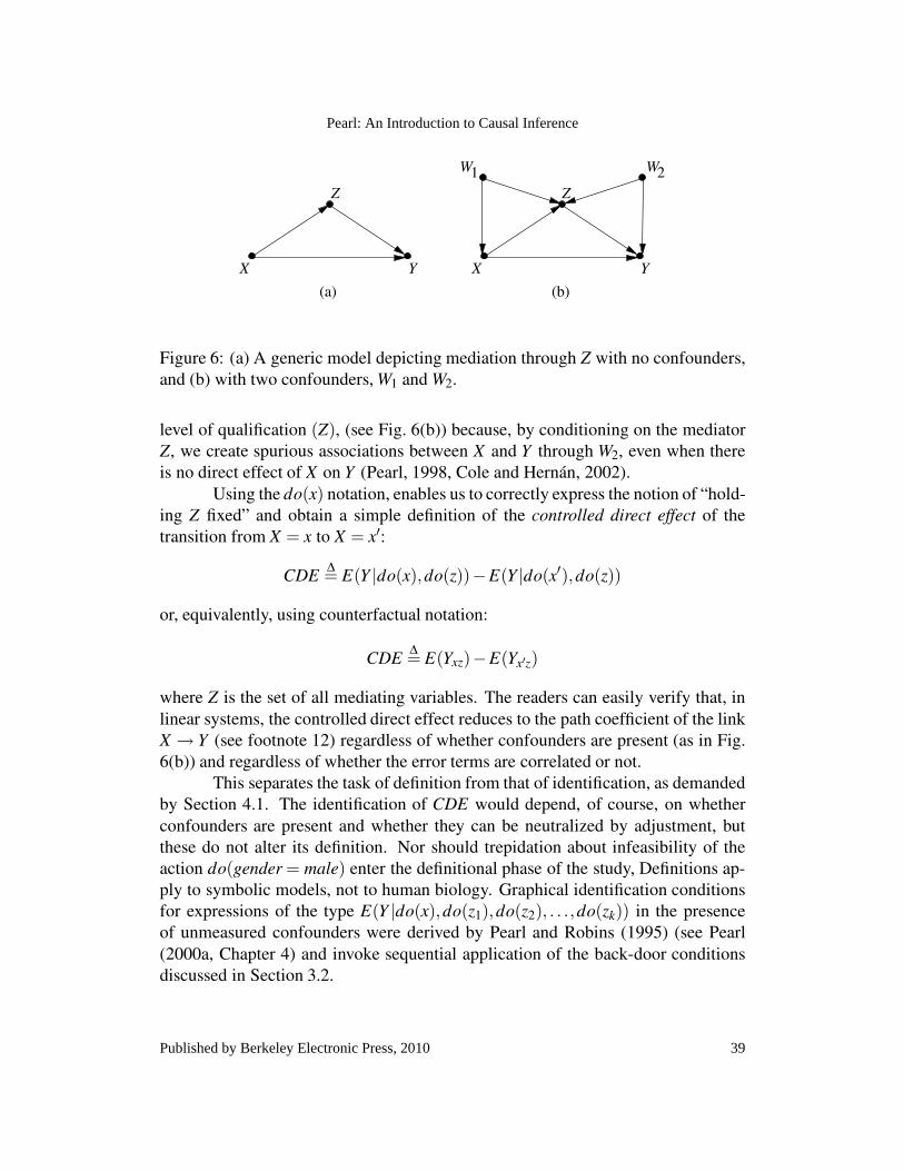
YXYX

W1 W2

(b)(a)

Z Z

Figure 6: (a) A generic model depicting mediation through Z with no confounders,

and (b) with two confounders, W1 and W2.

level of qualification (Z), (see Fig. 6(b)) because, by conditioning on the mediator

Z, we create spurious associations between X and Y through W2, even when there

is no direct effect of X on Y (Pearl, 1998, Cole and Hernan, 2002).

Using the do(x) notation, enables us to correctly express the notion of “hold-

ing Z fixed” and obtain a simple definition of the controlled direct effect of the

transition from X = x to X = x′:

CDE∆= E(Y |do(x),do(z))−E(Y |do(x′),do(z))

or, equivalently, using counterfactual notation:

CDE∆= E(Yxz)−E(Yx′z)

where Z is the set of all mediating variables. The readers can easily verify that, in

linear systems, the controlled direct effect reduces to the path coefficient of the link

X → Y (see footnote 12) regardless of whether confounders are present (as in Fig.

6(b)) and regardless of whether the error terms are correlated or not.

This separates the task of definition from that of identification, as demanded

by Section 4.1. The identification of CDE would depend, of course, on whether

confounders are present and whether they can be neutralized by adjustment, but

these do not alter its definition. Nor should trepidation about infeasibility of the

action do(gender = male) enter the definitional phase of the study, Definitions ap-

ply to symbolic models, not to human biology. Graphical identification conditions

for expressions of the type E(Y |do(x),do(z1),do(z2), . . .,do(zk)) in the presence

of unmeasured confounders were derived by Pearl and Robins (1995) (see Pearl

(2000a, Chapter 4) and invoke sequential application of the back-door conditions

discussed in Section 3.2.

39



6.1.3 Natural direct effects

In linear systems, the direct effect is fully specified by the path coefficient attached

to the link from X to Y ; therefore, the direct effect is independent of the values at

which we hold Z. In nonlinear systems, those values would, in general, modify the

effect of X on Y and thus should be chosen carefully to represent the target policy

under analysis. For example, it is not uncommon to find employers who prefer

males for the high-paying jobs (i.e., high z) and females for low-paying jobs (low

z).

When the direct effect is sensitive to the levels at which we hold Z, it is often

more meaningful to define the direct effect relative to some “natural” base-line level

that may vary from individual to individual, and represents the level of Z just before

the change in X . Conceptually, we can define the natural direct effect DEx,x′(Y )as the expected change in Y induced by changing X from x to x′ while keeping all

mediating factors constant at whatever value they would have obtained under do(x).This hypothetical change, which Robins and Greenland (1992) conceived and called

“pure” and Pearl (2001) formalized and analyzed under the rubric “natural,” mirrors

what lawmakers instruct us to consider in race or sex discrimination cases: “The

central question in any employment-discrimination case is whether the employer

would have taken the same action had the employee been of a different race (age,

sex, religion, national origin etc.) and everything else had been the same.” (In

Carson versus Bethlehem Steel Corp., 70 FEP Cases 921, 7th Cir. (1996)).

Extending the subscript notation to express nested counterfactuals, Pearl

(2001) gave a formal definition for the “natural direct effect”:

DEx,x′(Y ) = E(Yx′,Zx)−E(Yx). (42)

Here, Yx′,Zxrepresents the value that Y would attain under the operation of setting X

to x′ and, simultaneously, setting Z to whatever value it would have obtained under

the setting X = x. We see that DEx,x′(Y ), the natural direct effect of the transition

from x to x′, involves probabilities of nested counterfactuals and cannot be written

in terms of the do(x) operator. Therefore, the natural direct effect cannot in general

be identified, even with the help of ideal, controlled experiments (see footnote 8 for

intuitive explanation). However, aided by the surgical definition of Eq. (29) and the

notational power of nested counterfactuals, Pearl (2001) was nevertheless able to

show that, if certain assumptions of “no confounding” are deemed valid, the natural

direct effect can be reduced to

DEx,x′(Y ) = ∑z

[E(Y |do(x′, z))−E(Y |do(x, z))]P(z|do(x)). (43)

The intuition is simple; the natural direct effect is the weighted average of the con-

trolled direct effect, using the causal effect P(z|do(x)) as a weighing function.

40



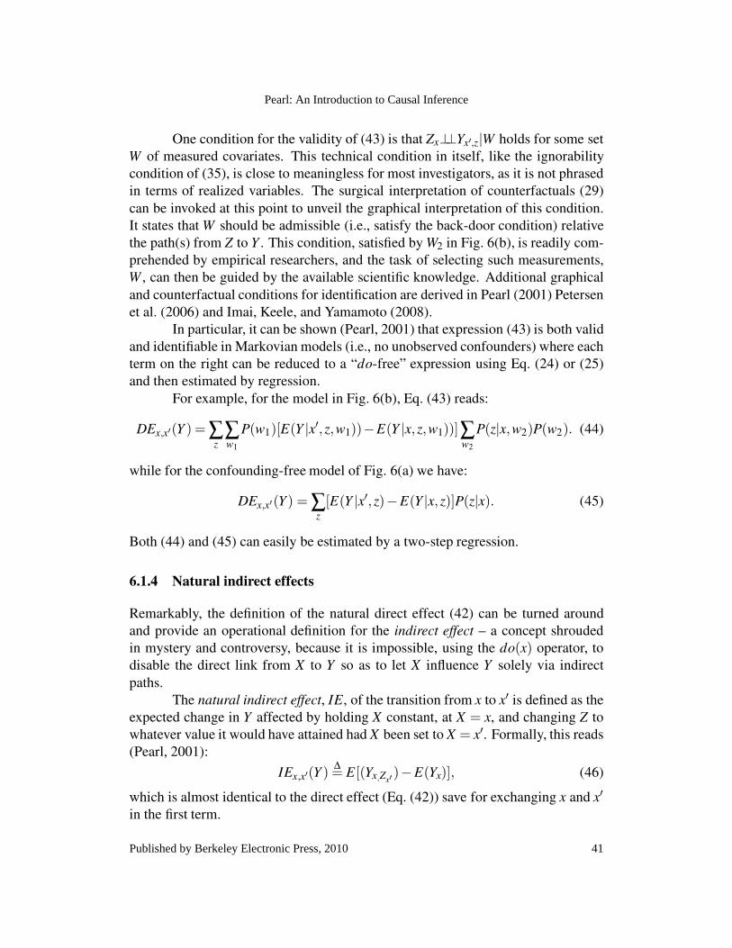
One condition for the validity of (43) is that Zx⊥⊥Yx′,z|W holds for some set

W of measured covariates. This technical condition in itself, like the ignorability

condition of (35), is close to meaningless for most investigators, as it is not phrased

in terms of realized variables. The surgical interpretation of counterfactuals (29)

can be invoked at this point to unveil the graphical interpretation of this condition.

It states that W should be admissible (i.e., satisfy the back-door condition) relative

the path(s) from Z to Y . This condition, satisfied by W2 in Fig. 6(b), is readily com-

prehended by empirical researchers, and the task of selecting such measurements,

W , can then be guided by the available scientific knowledge. Additional graphical

and counterfactual conditions for identification are derived in Pearl (2001) Petersen

et al. (2006) and Imai, Keele, and Yamamoto (2008).

In particular, it can be shown (Pearl, 2001) that expression (43) is both valid

and identifiable in Markovian models (i.e., no unobserved confounders) where each

term on the right can be reduced to a “do-free” expression using Eq. (24) or (25)

and then estimated by regression.

For example, for the model in Fig. 6(b), Eq. (43) reads:

DEx,x′(Y ) = ∑z

∑w1

P(w1)[E(Y |x′, z,w1))−E(Y |x, z,w1))]∑w2

P(z|x,w2)P(w2). (44)

while for the confounding-free model of Fig. 6(a) we have:

DEx,x′(Y) = ∑z

[E(Y |x′, z)−E(Y |x, z)]P(z|x). (45)

Both (44) and (45) can easily be estimated by a two-step regression.

6.1.4 Natural indirect effects

Remarkably, the definition of the natural direct effect (42) can be turned around

and provide an operational definition for the indirect effect – a concept shrouded

in mystery and controversy, because it is impossible, using the do(x) operator, to

disable the direct link from X to Y so as to let X influence Y solely via indirect

paths.

The natural indirect effect, IE, of the transition from x to x′ is defined as the

expected change in Y affected by holding X constant, at X = x, and changing Z to

whatever value it would have attained had X been set to X = x′. Formally, this reads

(Pearl, 2001):

IEx,x′(Y )∆= E[(Yx,Zx′

)−E(Yx)], (46)

which is almost identical to the direct effect (Eq. (42)) save for exchanging x and x′

in the first term.

41



Kaoru

Pencil

Kaoru

Pencil

Kaoru

Text Box

the natural direct effect is

Kaoru

Pencil

Kaoru

Pencil

Kaoru

Pencil

Kaoru

Text Box

"

Kaoru

Pencil

Kaoru

Pencil

Kaoru

Pencil

Kaoru

Pencil

Kaoru

Rectangle

Kaoru

Line

Kaoru

Line

Kaoru

Line

Kaoru

Pencil

Kaoru

Text Box

we have:

Kaoru

Pencil

Kaoru

Text Box

2

Kaoru

Text Box

2

Kaoru

Text Box

2

Kaoru

Text Box

2

Kaoru

Pencil

Kaoru

Text Box

1

Kaoru

Text Box

1

Kaoru

Text Box

w1,

Kaoru

Pencil

Kaoru

Pencil

Kaoru

Oval

Kaoru

Pencil

Kaoru

Pencil

Kaoru

Text Box

identifiability of DEx,x' (Y)

Kaoru

Pencil

Kaoru

Pencil

Kaoru

Line

Indeed, it can be shown that, in general, the total effect T E of a transition

is equal to the difference between the direct effect of that transition and the indirect

effect of the reverse transition. Formally,

T Ex,x′(Y )∆= E(Yx′−Yx) = DEx,x′(Y )− IEx′,x(Y ). (47)

In linear systems, where reversal of transitions amounts to negating the signs of

their effects, we have the standard additive formula

T Ex,x′(Y ) = DEx,x′(Y )+ IEx,x′(Y ). (48)

Since each term above is based on an independent operational definition, this equal-

ity constitutes a formal justification for the additive formula used routinely in linear

systems.

Note that, although it cannot be expressed in do-notation, the indirect effect

has clear policy-making implications. For example: in the hiring discrimination

context, a policy maker may be interested in predicting the gender mix in the work

force if gender bias is eliminated and all applicants are treated equally—say, the

same way that males are currently treated. This quantity will be given by the indirect

effect of gender on hiring, mediated by factors such as education and aptitude,

which may be gender-dependent.

More generally, a policy maker may be interested in the effect of issuing

a directive to a select set of subordinate employees, or in carefully controlling the

routing of messages in a network of interacting agents. Such applications motivate

the analysis of path-specific effects, that is, the effect of X on Y through a selected

set of paths (Avin, Shpitser, and Pearl, 2005).

In all these cases, the policy intervention invokes the selection of signals to

be sensed, rather than variables to be fixed. Pearl (2001) has suggested therefore

that signal sensing is more fundamental to the notion of causation than manipu-

lation; the latter being but a crude way of stimulating the former in experimental

setup. The mantra “No causation without manipulation” must be rejected. (See

(Pearl, 2009b, Section 11.4.5).)

It is remarkable that counterfactual quantities like DE and IE that could

not be expressed in terms of do(x) operators, and appear therefore void of empiri-

cal content, can, under certain conditions be estimated from empirical studies, and

serve to guide policies. Awareness of this potential should embolden researchers to

go through the definitional step of the study and freely articulate the target quan-

tity Q(M) in the language of science, i.e., counterfactuals, despite the seemingly

speculative nature of each assumption in the model (Pearl, 2000b).

42



6.2 The Mediation Formula: a simple solution to a thorny prob-

lem

This subsection demonstrates how the solution provided in equations (45) and (48)

can be applied to practical problems of assessing mediation effects in non-linear

models. We will use the simple mediation model of Fig. 6(a), where all error terms

(not shown explicitly) are assumed to be mutually independent, with the under-

standing that adjustment for appropriate sets of covariates W may be necessary to

achieve this independence and that integrals should replace summations when deal-

ing with continuous variables (Imai et al., 2008).

Combining (45) and (48), the expression for the indirect effect, IE, be-

comes:

IEx,x′(Y) = ∑z

E(Y |x, z)[P(z|x′)−P(z|x)] (49)

which provides a general formula for mediation effects, applicable to any nonlinear

system, any distribution (of U ), and any type of variables. Moreover, the formula is

readily estimable by regression. Owed to its generality and ubiquity, I will refer to

this expression as the “Mediation Formula.”

The Mediation Formula represents the average increase in the outcome Y

that the transition from X = x to X = x′ is expected to produce absent any direct

effect of X on Y . Though based on solid causal principles, it embodies no causal

assumption other than the generic mediation structure of Fig. 6(a). When the out-

come Y is binary (e.g., recovery, or hiring) the ratio (1− IE/TE) represents the

fraction of responding individuals who owe their response to direct paths, while

(1−DE/T E) represents the fraction who owe their response to Z-mediated paths.

The Mediation Formula tells us that IE depends only on the expectation

of the counterfactual Yxz, not on its functional form fY (x, z,uY ) or its distribution

P(Yxz = y). It calls therefore for a two-step regression which, in principle, can be

performed non-parametrically. In the first step we regress Y on X and Z, and obtain

the estimate

g(x, z) = E(Y |x, z)

for every (x, z) cell. In the second step we estimate the expectation of g(x, z) condi-

tional on X = x′ and X = x, respectively, and take the difference:

IEx,x′(Y ) = Ez(g(x, z)|x′)−Ez(g(x, z)|x)

Nonparametric estimation is not always practical. When Z consists of a

vector of several mediators, the dimensionality of the problem would prohibit the

estimation of E(Y |x, z) for every (x, z) cell, and the need arises to use parametric

approximation. We can then choose any convenient parametric form for E(Y |x, z)

43



(e.g., linear, logit, probit), estimate the parameters separately (e.g., by regression

or maximum likelihood methods), insert the parametric approximation into (49)

and estimate its two conditional expectations (over z) to get the mediated effect

(VanderWeele, 2009).

Let us examine what the Mediation Formula yields when applied to both

linear and non-linear versions of model 6(a). In the linear case, the structural model

reads:

x = uX

z = bxx+uZ (50)

y = cxx+ czz+uY

Computing the conditional expectation in (49) gives

E(Y |x, z) = E(cxx+ czz+uY ) = cxx+ czz

and yields

IEx,x′(Y ) = ∑z

(cxx+ czz)[P(z|x′)−P(z|x)].

= cz[E(Z|x′)−E(Z|x)] (51)

= (x′− x)(czbx) (52)

= (x′− x)(b− cx) (53)

where b is the total effect coefficient, b = (E(Y |x′)−E(Y |x))/(x′− x) = cx + czbx.

We thus obtained the standard expressions for indirect effects in linear sys-

tems, which can be estimated either as a difference in two regression coefficients

(Eq. 53) or a product of two regression coefficients (Eq. 52), with Y regressed on

both X and Z. (see (MacKinnon et al., 2007b)). These two strategies do not gener-

alize to non-linear system as we shall see next.

Suppose we apply (49) to a non-linear process (Fig. 7) in which X ,Y , and Z

are binary variables, and Y and Z are given by the Boolean formula

Y = AND (x,ex)∨ AND (z,ez) x, z,ex,ez = 0,1

z = AND (x,exz) z,exz = 0,1

Such disjunctive interaction would describe, for example, a disease Y that would

be triggered either by X directly, if enabled by ex, or by Z, if enabled by ez. Let

us further assume that ex,ez and exz are three independent Bernoulli variables with

probabilities px, pz, and pxz, respectively.

44



OR

AND ANDZ

xe p(~ )x

e p(~ )zz

XAND Y

(~ )e pzx xz

Figure 7: Stochastic non-linear model of mediation. All variables are binary.

As investigators, we are not aware, of course, of these underlying mecha-

nisms; all we know is that X ,Y , and Z are binary, that Z is hypothesized to be a

mediator, and that the assumption of nonconfoundedness permits us to use the Me-

diation Formula (49) for estimating the Z-mediated effect of X on Y . Assume that

our plan is to conduct a nonparametric estimation of the terms in (49) over a very

large sample drawn from P(x,y.z); it is interesting to ask what the asymptotic value

of the Mediation Formula would be, as a function of the model parameters: px, pz,

and pxz.

From knowledge of the underlying mechanism, we have:

P(Z = 1|x) = pxzx x = 0,1

P(Y = 1|x, z) = pxx+ pzz− px pzxz x, z = 0,1

Therefore,

E(Z|x) = pxzx x = 0,1

E(Y |x, z) = xpx + zpz− xzpxpz x, z = 0,1

E(Y |x) = ∑z E(Y |x, z)P(z|x)= xpx +(pz− xpxpz)E(Z|x)= x(px + pxzpz− xpxpz pxz) x = 0,1

Taking x = 0,x′ = 1 and substituting these expressions in (45), (48), and

(49) yields

IE(Y) = pz pxz (54)

DE(Y ) = px (55)

T E(Y ) = pz pxz + px + pxpz pxz (56)

Two observations are worth noting. First, we see that, despite the non-linear

interaction between the two causal paths, the parameters of one do not influence on

45



the causal effect mediated by the other. Second, the total effect is not the sum of the

direct and indirect effects. Instead, we have:

T E = DE + IE−DE · IE

which means that a fraction DE ·IE/T E of outcome cases triggered by the transition

from X = 0 to X = 1 are triggered simultaneously, through both causal paths, and

would have been triggered even if one of the paths was disabled.

Now assume that we choose to approximate E(Y |x, z) by the linear expres-

sion

g(x, z) = a0 +a1x+a2z. (57)

After fitting the a’s parameters to the data (e.g., by OLS) and substituting in (49)

one would obtain

IEx,x′(Y ) = ∑z(a0 +a1x+a2z)[P(z|x′)−P(z|x)]= a2[E(Z|x′)−E(Z|x)]

(58)

which holds whenever we use the approximation in (57), regardless of the underly-

ing mechanism.

If the correct data-generating process was the linear model of (50), we

would obtain the expected estimates a2 = cz,E(z|x′)−E(z|x′) = bx(x′− x) and

IEx,x′(Y ) = bxcz(x′− x).

If however we were to apply the approximation in (57) to data generated by

the nonlinear model of Fig. 7, a distorted solution would ensue; a2 would evaluate

to

a2 = ∑x[E(Y |x, z = 1)−E(Y |x, z = 0)]P(x)= P(x = 1)[E(Y |x = 1, z = 1)−E(Y |x = 1, z = 0)]= P(x = 1)[(px + pz− pxpz)− px]= P(x = 1)pz(1− px),

E(z|x′)−E(z|x) would evaluate to pxz(x′−x), and (58) would yield the approxima-

tion

IEx,x′(Y) = a2[E(Z|x′)−E(Z|x)]= pxzP(x = 1)pz(1− px)

(59)

We see immediately that the result differs from the correct value pz pxz de-

rived in (54). Whereas the approximate value depends on P(x = 1), the correct

value shows no such dependence, and rightly so; no causal effect should depend on

the probability of the causal variable.

46



Fortunately, the analysis permits us to examine under what condition the

distortion would be significant. Comparing (59) and (54) reveals that the approxi-

mate method always underestimates the indirect effect and the distortion is minimal

for high values of P(x = 1) and (1− px).Had we chosen to include an interaction term in the approximation of

E(Y |x, z), the correct result would obtain. To witness, writing

E(Y |x, z) = a0 +a1x+a2z+a3xz,

a2 would evaluate to pz, a3 to px pz, and the correct result obtains through:

IEx,x′(Y ) = ∑z

(a0 +a1x+a2z+a3xz)[P(z|x′)−P(z|x)]

= (a2 +a3x)[E(Z|x′)−E(Z|x)]

= (a2 +a3x)pxz(x′− x)

= (pz− pxpzx)pxz(x′− x)

We see that, in addition to providing causally-sound estimates for mediation

effects, the Mediation Formula also enables researchers to evaluate analytically the

effectiveness of various parametric specifications relative to any assumed model.

This type of analytical “sensitivity analysis” has been used extensively in statistics

for parameter estimation, but could not be applied to mediation analysis, owed to the

absence of an objective target quantity that captures the notion of indirect effect in

both linear and non-linear systems, free of parametric assumptions. The Mediation

Formula of Eq. (49) explicates this target quantity formally, and casts it in terms of

estimable quantities.

The derivation of the Mediation Formula was facilitated by taking seriously

the four steps of the structural methodology (Section 4) together with the graphical-

counterfactual-structural symbiosis spawned by the surgical interpretation of coun-

terfactuals (Eq. (29)).

In contrast, when the mediation problem is approached from an exclusivist

potential-outcome viewpoint, void of the structural guidance of Eq. (29), counterin-

tuitive definitions ensue, carrying the label “principal stratification” (Rubin, 2004,

2005), which are at variance with common understanding of direct and indirect ef-

fects. For example, the direct effect is definable only in units absent of indirect

effects. This means that a grandfather would be deemed to have no direct effect

on his grandson’s behavior in families where he has had some effect on the father.

This precludes from the analysis all typical families, in which a father and a grand-

father have simultaneous, complementary influences on children’s upbringing. In

linear systems, to take an even sharper example, the direct effect would be unde-

fined whenever indirect paths exist from the cause to its effect. The emergence of

47



such paradoxical conclusions underscores the wisdom, if not necessity of a symbi-

otic analysis, in which the counterfactual notation Yx(u) is governed by its structural

definition, Eq. (29).19

6.3 Causes of effects and probabilities of causation

The likelihood that one event was the cause of another guides much of what we

understand about the world (and how we act in it). For example, knowing whether

it was the aspirin that cured my headache or the TV program I was watching would

surely affect my future use of aspirin. Likewise, to take an example from common

judicial standard, judgment in favor of a plaintiff should be made if and only if it

is “more probable than not” that the damage would not have occurred but for the

defendant’s action (Robertson, 1997).

These two examples fall under the category of “causes of effects” because

they concern situations in which we observe both the effect, Y = y, and the putative

cause X = x and we are asked to assess, counterfactually, whether the former would

have occurred absent the latter.

We have remarked earlier (footnote 8) that counterfactual probabilities con-

ditioned on the outcome cannot in general be identified from observational or even

experimental studies. This does not mean however that such probabilities are use-

less or void of empirical content; the structural perspective may guide us in fact

toward discovering the conditions under which they can be assessed from data, thus

defining the empirical content of these counterfactuals.

Following the 4-step process of structural methodology – define, assume,

identify, and estimate – our first step is to express the target quantity in counter-

factual notation and verify that it is well defined, namely, that it can be computed

unambiguously from any fully-specified causal model.

In our case, this step is simple. Assuming binary events, with X = x and

Y = y representing treatment and outcome, respectively, and X = x′, Y = y′ their

negations, our target quantity can be formulated directly from the English sentence:

“Find the probability that Y would be y′ had X been x′, given that, in

reality, Y is actually y and X is x,”

to give:

PN(x,y) = P(Yx′ = y′|X = x,Y = y) (60)

19Such symbiosis is now standard in epidemiology research (Robins, 2001, Petersen et al., 2006,

VanderWeele and Robins, 2007, Hafeman and Schwartz, 2009, VanderWeele, 2009) and is making

its way slowly toward the social and behavioral sciences.

48



This counterfactual quantity, which Robins and Greenland (1989b) named

“probability of causation” and Pearl (2000a, p. 296) named “probability of neces-

sity” (PN), to be distinguished from two other nuances of “causation,” is certainly

computable from any fully specified structural model, i.e., one in which P(u) and all

functional relationships are given. This follows from the fact that every structural

model defines a joint distribution of counterfactuals, through Eq. (29).

Having written a formal expression for PN, Eq. (60), we can move on to

the formulation and identification phases and ask what assumptions would permit

us to identify PN from empirical studies, be they observational, experimental or a

combination thereof.

This problem was analyzed in Pearl (2000a, Chapter 9) and yielded the

following results:

Theorem 4 If Y is monotonic relative to X, i.e., Y1(u)≥ Y0(u), then PN is identifi-

able whenever the causal effect P(y|do(x)) is identifiable and, moreover,

PN =P(y|x)−P(y|x′)

P(y|x)+

P(y|x′)−P(y|do(x′))

P(x,y). (61)

The first term on the r.h.s. of (61) is the familiar excess risk ratio (ERR) that epi-

demiologists have been using as a surrogate for PN in court cases (Cole, 1997,

Robins and Greenland, 1989b). The second term represents the correction needed

to account for confounding bias, that is, P(y|do(x′)) 6= P(y|x′).This suggests that monotonicity and unconfoundedness were tacitly assumed

by the many authors who proposed or derived ERR as a measure for the “fraction

of exposed cases that are attributable to the exposure” (Greenland, 1999).

Equation (61) thus provides a more refined measure of causation, which can

be used in situations where the causal effect P(y|do(x)) can be estimated from either

randomized trials or graph-assisted observational studies (e.g., through Theorem 3

or Eq. (25)). It can also be shown (Tian and Pearl, 2000) that the expression in

(61) provides a lower bound for PN in the general, nonmonotonic case. (See also

(Robins and Greenland, 1989a).) In particular, the tight upper and lower bounds on

PN are given by:

max{

0,P(y)−P(y|do(x′))

P(x,y)

}

≤ PN ≤min{

1,P(y′|do(x′))−P(x′,y′)

P(x,y)

}

(62)

It is worth noting that, in drug related litigation, it is not uncommon to ob-

tain data from both experimental and observational studies. The former is usually

available at the manufacturer or the agency that approved the drug for distribution

(e.g., FDA), while the latter is easy to obtain by random surveys of the population.

49



In such cases, the standard lower bound used by epidemiologists to establish le-

gal responsibility, the Excess Risk Ratio, can be improved substantially using the

corrective term of Eq. (61). Likewise, the upper bound of Eq. (62) can be used to

exonerate drug-makers from legal responsibility. Cai and Kuroki (2006) analyzed

the statistical properties of PN.

Pearl (2000a, p. 302) shows that combining data from experimental and

observational studies which, taken separately, may indicate no causal relations be-

tween X and Y , can nevertheless bring the lower bound of Eq. (62) to unity, thus

implying causation with probability one.

Such extreme results dispel all fears and trepidations concerning the empiri-

cal content of counterfactuals (Dawid, 2000, Pearl, 2000b). They demonstrate that a

quantity PN which at first glance appears to be hypothetical, ill-defined, untestable

and, hence, unworthy of scientific analysis is nevertheless definable, testable and,

in certain cases, even identifiable. Moreover, the fact that, under certain combina-

tion of data, and making no assumptions whatsoever, an important legal claim such

as “the plaintiff would be alive had he not taken the drug” can be ascertained with

probability approaching one, is a remarkable tribute to formal analysis.

Another counterfactual quantity that has been fully characterized recently is

the Effect of Treatment on the Treated (ETT):

ET T = P(Yx = y|X = x′)

ETT has been used in econometrics to evaluate the effectiveness of social programs

on their participants (Heckman, 1992) and has long been the target of research

in epidemiology, where it came to be known as “the effect of exposure on the

exposed,” or “standardized morbidity” (Miettinen, 1974; Greenland and Robins,

1986).

Shpitser and Pearl (2009) have derived a complete characterization of those

models in which ETT can be identified from either experimental or observational

studies. They have shown that, despite its blatant counterfactual character, (e.g.,

“I just took an aspirin, perhaps I shouldn’t have?”) ETT can be evaluated from

experimental studies in many, though not all cases. It can also be evaluated from

observational studies whenever a sufficient set of covariates can be measured that

satisfies the back-door criterion and, more generally, in a wide class of graphs that

permit the identification of conditional interventions.

These results further illuminate the empirical content of counterfactuals and

their essential role in causal analysis. They prove once again the triumph of logic

and analysis over traditions that a-priori exclude from the analysis quantities that are

not testable in isolation. Most of all, they demonstrate the effectiveness and viability

of the scientific approach to causation whereby the dominant paradigm is to model

the activities of Nature, rather than those of the experimenter. In contrast to the

50



ruling paradigm of conservative statistics, we begin with relationships that we know

in advance will never be estimated, tested or falsified. Only after assembling a host

of such relationships and judging them to faithfully represent our theory about how

Nature operates, we ask whether the parameter of interest, crisply defined in terms

of those theoretical relationships, can be estimated consistently from empirical data

and how. It often does, to the credit of progressive statistics.

7 Conclusions

Traditional statistics is strong in devising ways of describing data and inferring

distributional parameters from sample. Causal inference requires two additional

ingredients: a science-friendly language for articulating causal knowledge, and a

mathematical machinery for processing that knowledge, combining it with data

and drawing new causal conclusions about a phenomenon. This paper surveys re-

cent advances in causal analysis from the unifying perspective of the structural the-

ory of causation and shows how statistical methods can be supplemented with the

needed ingredients. The theory invokes non-parametric structural equations mod-

els as a formal and meaningful language for defining causal quantities, formulating

causal assumptions, testing identifiability, and explicating many concepts used in

causal discourse. These include: randomization, intervention, direct and indirect

effects, confounding, counterfactuals, and attribution. The algebraic component

of the structural language coincides with the potential-outcome framework, and its

graphical component embraces Wright’s method of path diagrams. When unified

and synthesized, the two components offer statistical investigators a powerful and

comprehensive methodology for empirical research.

References

Angrist, J., G. Imbens, and D. Rubin (1996): “Identification of causal effects us-

ing instrumental variables (with comments),” Journal of the American Statistical

Association, 91, 444–472.

Arah, O. (2008): “The role of causal reasoning in understanding Simp-

son’s paradox, Lord’s paradox, and the suppression effect: Covariate se-

lection in the analysis of observational studies,” Emerging Themes in

Epidemiology, 4, doi:10.1186/1742–7622–5–5, online at <http://www.ete-

online.com/content/5/1/5>.

Arjas, E. and J. Parner (2004): “Causal reasoning from longitudinal data,” Scandi-

navian Journal of Statistics, 31, 171–187.

51



Avin, C., I. Shpitser, and J. Pearl (2005): “Identifiability of path-specific effects,”

in Proceedings of the Nineteenth International Joint Conference on Artificial In-

telligence IJCAI-05, Edinburgh, UK: Morgan-Kaufmann Publishers, 357–363.

Balke, A. and J. Pearl (1995): “Counterfactuals and policy analysis in structural

models,” in P. Besnard and S. Hanks, eds., Uncertainty in Artificial Intelligence

11, San Francisco: Morgan Kaufmann, 11–18.

Balke, A. and J. Pearl (1997): “Bounds on treatment effects from studies with im-

perfect compliance,” Journal of the American Statistical Association, 92, 1172–

1176.

Baron, R. and D. Kenny (1986): “The moderator-mediator variable distinction in

social psychological research: Conceptual, strategic, and statistical considera-

tions,” Journal of Personality and Social Psychology, 51, 1173–1182.

Berkson, J. (1946): “Limitations of the application of fourfold table analysis to

hospital data,” Biometrics Bulletin, 2, 47–53.

Bollen, K. (1989): Structural Equations with Latent Variables, New York: John

Wiley.

Brent, R. and L. Lok (2005): “A fishing buddy for hypothesis generators,” Science,

308, 523–529.

Cai, Z. and M. Kuroki (2006): “Variance estimators for three ‘probabilities of cau-

sation’,” Risk Analysis, 25, 1611–1620.

Cai, Z. and M. Kuroki (2008): “On identifying total effects in the presence of latent

variables and selection bias,” in D. A. McAllester and P. Myllymaki, eds., Un-

certainty in Artificial Intelligence, Proceedings of the Twenty-Fourth Conference,

Arlington, VA: AUAI, 62–69.

Cartwright, N. (2007): Hunting Causes and Using Them: Approaches in Philoso-

phy and Economics, New York, NY: Cambridge University Press.

Chalak, K. and H. White (2006): “An extended class of instrumental variables for

the estimation of causal effects,” Technical Report Discussion Paper, UCSD, De-

partment of Economics.

Chickering, D. and J. Pearl (1997): “A clinician’s tool for analyzing non-

compliance,” Computing Science and Statistics, 29, 424–431.

Cole, P. (1997): “Causality in epidemiology, health policy, and law,” Journal of

Marketing Research, 27, 10279–10285.

Cole, S. and M. Hernan (2002): “Fallibility in estimating direct effects,” Interna-

tional Journal of Epidemiology, 31, 163–165.

Cox, D. (1958): The Planning of Experiments, NY: John Wiley and Sons.

Cox, D. and N. Wermuth (2004): “Causality: A statistical view,” International

Statistical Review, 72, 285–305.

Dawid, A. (1979): “Conditional independence in statistical theory,” Journal of the

Royal Statistical Society, Series B, 41, 1–31.

52



Dawid, A. (2000): “Causal inference without counterfactuals (with comments and

rejoinder),” Journal of the American Statistical Association, 95, 407–448.

Dawid, A. (2002): “Influence diagrams for causal modelling and inference,” Inter-

national Statistical Review, 70, 161–189.

Duncan, O. (1975): Introduction to Structural Equation Models, New York: Aca-

demic Press.

Eells, E. (1991): Probabilistic Causality, Cambridge, MA: Cambridge University

Press.

Frangakis, C. and D. Rubin (2002): “Principal stratification in causal inference,”

Biometrics, 1, 21–29.

Glymour, M. and S. Greenland (2008): “Causal diagrams,” in K. Rothman,

S. Greenland, and T. Lash, eds., Modern Epidemiology, Philadelphia, PA: Lip-

pincott Williams & Wilkins, 3rd edition, 183–209.

Goldberger, A. (1972): “Structural equation models in the social sciences,” Econo-

metrica: Journal of the Econometric Society, 40, 979–1001.

Goldberger, A. (1973): “Structural equation models: An overview,” in A. Gold-

berger and O. Duncan, eds., Structural Equation Models in the Social Sciences,

New York, NY: Seminar Press, 1–18.

Greenland, S. (1999): “Relation of probability of causation, relative risk, and dou-

bling dose: A methodologic error that has become a social problem,” American

Journal of Public Health, 89, 1166–1169.

Greenland, S., J. Pearl, and J. Robins (1999): “Causal diagrams for epidemiologic

research,” Epidemiology, 10, 37–48.

Greenland, S. and J. Robins (1986): “Identifiability, exchangeability, and epidemi-

ological confounding,” International Journal of Epidemiology, 15, 413–419.

Haavelmo, T. (1943): “The statistical implications of a system of simultaneous

equations,” Econometrica, 11, 1–12, reprinted in D.F. Hendry and M.S. Morgan

(Eds.), The Foundations of Econometric Analysis, Cambridge University Press,

477–490, 1995.

Hafeman, D. and S. Schwartz (2009): “Opening the black box: A motivation for the

assessment of mediation,” International Journal of Epidemiology, 3, 838–845.

Halpern, J. (1998): “Axiomatizing causal reasoning,” in G. Cooper and S. Moral,

eds., Uncertainty in Artificial Intelligence, San Francisco, CA: Morgan Kauf-

mann, 202–210, also, Journal of Artificial Intelligence Research 12:3, 17–37,

2000.

Heckman, J. (1992): “Randomization and social policy evaluation,” in C. Manski

and I. Garfinkle, eds., Evaluations: Welfare and Training Programs, Cambridge,

MA: Harvard University Press, 201–230.

Heckman, J. (2005): “The scientific model of causality,” Sociological Methodology,

35, 1–97.

53



Heckman, J. (2008): “Econometric causality,” International Statistical Review, 76,

1–27.

Heckman, J. and S. Navarro-Lozano (2004): “Using matching, instrumental vari-

ables, and control functions to estimate economic choice models,” The Review of

Economics and Statistics, 86, 30–57.

Heckman, J. and E. Vytlacil (2005): “Structural equations, treatment effects and

econometric policy evaluation,” Econometrica, 73, 669–738.

Hernan, M. and S. Cole (2009): “Invited commentary: Causal diagrams and mea-

surement bias,” American Journal of Epidemiology, 170, 959–962.

Holland, P. (1988): “Causal inference, path analysis, and recursive structural equa-

tions models,” in C. Clogg, ed., Sociological Methodology, Washington, D.C.:

American Sociological Association, 449–484.

Hurwicz, L. (1950): “Generalization of the concept of identification,” in T. Koop-

mans, ed., Statistical Inference in Dynamic Economic Models, Cowles Commis-

sion, Monograph 10, New York: Wiley, 245–257.

Imai, K., L. Keele, and T. Yamamoto (2008): “Identification, inference, and sen-

sitivity analysis for causal mediation effects,” Technical report, Department of

Politics, Princton University.

Imbens, G. and J. Wooldridge (2009): “Recent developments in the econometrics

of program evaluation,” Journal of Economic Literature, 47, 5–86.

Judd, C. and D. Kenny (1981): “Process analysis: Estimating mediation in treat-

ment evaluations,” Evaluation Review, 5, 602–619.

Kaufman, S., J. Kaufman, and R. MacLenose (2009): “Analytic bounds on causal

risk differences in directed acyclic graphs involving three observed binary vari-

ables,” Journal of Statistical Planning and Inference, 139, 3473–3487.

Kiiveri, H., T. Speed, and J. Carlin (1984): “Recursive causal models,” Journal of

Australian Math Society, 36, 30–52.

Koopmans, T. (1953): “Identification problems in econometric model construc-

tion,” in W. Hood and T. Koopmans, eds., Studies in Econometric Method, New

York: Wiley, 27–48.

Kuroki, M. and M. Miyakawa (1999): “Identifiability criteria for causal effects of

joint interventions,” Journal of the Royal Statistical Society, 29, 105–117.

Lauritzen, S. (1996): Graphical Models, Oxford: Clarendon Press.

Lauritzen, S. (2001): “Causal inference from graphical models,” in D. Cox and

C. Kluppelberg, eds., Complex Stochastic Systems, Boca Raton, FL: Chapman

and Hall/CRC Press, 63–107.

Lindley, D. (2002): “Seeing and doing: The concept of causation,” International

Statistical Review, 70, 191–214.

MacKinnon, D., A. Fairchild, and M. Fritz (2007a): “Mediation analysis,” Annual

Review of Psychology, 58, 593–614.

54



MacKinnon, D., C. Lockwood, C. Brown, W. Wang, and J. Hoffman (2007b): “The

intermediate endpoint effect in logistic and probit regression,” Clinical Trials, 4,

499–513.

Manski, C. (1990): “Nonparametric bounds on treatment effects,” American Eco-

nomic Review, Papers and Proceedings, 80, 319–323.

Marschak, J. (1950): “Statistical inference in economics,” in T. Koopmans, ed., Sta-

tistical Inference in Dynamic Economic Models, New York: Wiley, 1–50, cowles

Commission for Research in Economics, Monograph 10.

Meek, C. and C. Glymour (1994): “Conditioning and intervening,” British Journal

of Philosophy Science, 45, 1001–1021.

Miettinen, O. (1974): “Proportion of disease caused or prevented by a given expo-

sure, trait, or intervention,” Journal of Epidemiology, 99, 325–332.

Morgan, S. and C. Winship (2007): Counterfactuals and Causal Inference: Meth-

ods and Principles for Social Research (Analytical Methods for Social Research),

New York, NY: Cambridge University Press.

Muller, D., C. Judd, and V. Yzerbyt (2005): “When moderation is mediated and

mediation is moderated,” Journal of Personality and Social Psychology, 89, 852–

863.

Neyman, J. (1923): “On the application of probability theory to agricultural exper-

iments. Essay on principles. Section 9,” Statistical Science, 5, 465–480.

Pearl, J. (1988): Probabilistic Reasoning in Intelligent Systems, San Mateo, CA:

Morgan Kaufmann.

Pearl, J. (1993a): “Comment: Graphical models, causality, and intervention,” Sta-

tistical Science, 8, 266–269.

Pearl, J. (1993b): “Mediating instrumental variables,” Technical Report R-210,

<http://ftp.cs.ucla.edu/pub/stat ser/R210.pdf>, Department of Computer Sci-

ence, University of California, Los Angeles.

Pearl, J. (1995): “Causal diagrams for empirical research,” Biometrika, 82, 669–

710.

Pearl, J. (1998): “Graphs, causality, and structural equation models,” Sociological

Methods and Research, 27, 226–284.

Pearl, J. (2000a): Causality: Models, Reasoning, and Inference, New York: Cam-

bridge University Press, second ed., 2009.

Pearl, J. (2000b): “Comment on A.P. Dawid’s, Causal inference without counter-

factuals,” Journal of the American Statistical Association, 95, 428–431.

Pearl, J. (2001): “Direct and indirect effects,” in Proceedings of the Seventeenth

Conference on Uncertainty in Artificial Intelligence, San Francisco, CA: Morgan

Kaufmann, 411–420.

Pearl, J. (2004): “Robustness of causal claims,” in M. Chickering and J. Halpern,

eds., Proceedings of the Twentieth Conference Uncertainty in Artificial Intelli-

55



gence, Arlington, VA: AUAI Press, 446–453.

Pearl, J. (2009a): “Causal inference in statistics: An overview,” Statistics Surveys,

3, 96–146, <http://www.i-journals.org/ss/viewarticle.php?id=57>.

Pearl, J. (2009b): Causality: Models, Reasoning, and Inference, New York: Cam-

bridge University Press, second edition.

Pearl, J. (2009c): “Letter to the editor: Remarks on the method

of propensity scores,” Statistics in Medicine, 28, 1415–1416,

<http://ftp.cs.ucla.edu/pub/stat ser/r345-sim.pdf>.

Pearl, J. (2009d): “Myth, confusion, and science in causal analysis,” Technical

Report R-348, Department of Computer Science, University of California, Los

Angeles, CA, <http://ftp.cs.ucla.edu/pub/stat ser/r348.pdf>.

Pearl, J. (2009e): “On a class of bias-amplifying covariates that endanger effect es-

timates,” Technical Report R-346, Department of Computer Science, University

of California, Los Angeles, CA, <http://ftp.cs.ucla.edu/pub/stat ser/r346.pdf>.

Pearl, J. (2009f): “On measurement bias in causal inference,” Technical Report

R-357, <http://ftp.cs.ucla.edu/pub/stat ser/r357.pdf>, Department of Computer

Science, University of California, Los Angeles.

Pearl, J. and A. Paz (2009): “Confounding equivalence in observational studies,”

Technical Report R-343, Department of Computer Science, University of Cali-

fornia, Los Angeles, CA, <http://ftp.cs.ucla.edu/pub/stat ser/r343.pdf>.

Pearl, J. and J. Robins (1995): “Probabilistic evaluation of sequential plans from

causal models with hidden variables,” in P. Besnard and S. Hanks, eds., Uncer-

tainty in Artificial Intelligence 11, San Francisco: Morgan Kaufmann, 444–453.

Pearl, J. and T. Verma (1991): “A theory of inferred causation,” in J. Allen, R. Fikes,

and E. Sandewall, eds., Principles of Knowledge Representation and Reasoning:

Proceedings of the Second International Conference, San Mateo, CA: Morgan

Kaufmann, 441–452.

Petersen, M., S. Sinisi, and M. van der Laan (2006): “Estimation of direct causal

effects,” Epidemiology, 17, 276–284.

Richard, J. (1980): “Models with several regimes and changes in exogeneity,” Re-

view of Economic Studies, 47, 1–20.

Robertson, D. (1997): “The common sense of cause in fact,” Texas Law Review, 75,

1765–1800.

Robins, J. (1986): “A new approach to causal inference in mortality studies with

a sustained exposure period – applications to control of the healthy workers sur-

vivor effect,” Mathematical Modeling, 7, 1393–1512.

Robins, J. (1987): “A graphical approach to the identification and estimation of

causal parameters in mortality studies with sustained exposure periods,” Journal

of Chronic Diseases, 40, 139S–161S.

56



Robins, J. (1989): “The analysis of randomized and non-randomized aids treat-

ment trials using a new approach to causal inference in longitudinal studies,” in

L. Sechrest, H. Freeman, and A. Mulley, eds., Health Service Research Method-

ology: A Focus on AIDS, Washington, D.C.: NCHSR, U.S. Public Health Ser-

vice, 113–159.

Robins, J. (1999): “Testing and estimation of directed effects by reparameterizing

directed acyclic with structural nested models,” in C. Glymour and G. Cooper,

eds., Computation, Causation, and Discovery, Cambridge, MA: AAAI/MIT

Press, 349–405.

Robins, J. (2001): “Data, design, and background knowledge in etiologic infer-

ence,” Epidemiology, 12, 313–320.

Robins, J. and S. Greenland (1989a): “Estimability and estimation of excess and

etiologic fractions,” Statistics in Medicine, 8, 845–859.

Robins, J. and S. Greenland (1989b): “The probability of causation under a stochas-

tic model for individual risk,” Biometrics, 45, 1125–1138.

Robins, J. and S. Greenland (1992): “Identifiability and exchangeability for direct

and indirect effects,” Epidemiology, 3, 143–155.

Rosenbaum, P. (2002): Observational Studies, New York: Springer-Verlag, second

edition.

Rosenbaum, P. and D. Rubin (1983): “The central role of propensity score in ob-

servational studies for causal effects,” Biometrika, 70, 41–55.

Rothman, K. (1976): “Causes,” American Journal of Epidemiology, 104, 587–592.

Rubin, D. (1974): “Estimating causal effects of treatments in randomized and non-

randomized studies,” Journal of Educational Psychology, 66, 688–701.

Rubin, D. (2004): “Direct and indirect causal effects via potential outcomes,” Scan-

dinavian Journal of Statistics, 31, 161–170.

Rubin, D. (2005): “Causal inference using potential outcomes: Design, modeling,

decisions,” Journal of the American Statistical Association, 100, 322–331.

Rubin, D. (2007): “The design versus the analysis of observational studies for

causal effects: Parallels with the design of randomized trials,” Statistics in

Medicine, 26, 20–36.

Rubin, D. (2009): “Author’s reply: Should observational studies be designed to al-

low lack of balance in covariate distributions across treatment group?” Statistics

in Medicine, 28, 1420–1423.

Shpitser, I. and J. Pearl (2006): “Identification of conditional interventional dis-

tributions,” in R. Dechter and T. Richardson, eds., Proceedings of the Twenty-

Second Conference on Uncertainty in Artificial Intelligence, Corvallis, OR:

AUAI Press, 437–444.

Shpitser, I. and J. Pearl (2008): “Dormant independence,” in Proceedings of the

Twenty-Third Conference on Artificial Intelligence, Menlo Park, CA: AAAI

57



Press, 1081–1087.

Shpitser, I. and J. Pearl (2009): “Effects of treatment on the treated: Identification

and generalization,” in Proceedings of the Twenty-Fifth Conference on Uncer-

tainty in Artificial Intelligence, Montreal, Quebec: AUAI Press.

Shrier, I. (2009): “Letter to the editor: Propensity scores,”

Statistics in Medicine, 28, 1317–1318, see also Pearl 2009

<http://ftp.cs.ucla.edu/pub/stat ser/r348.pdf>.

Shrout, P. and N. Bolger (2002): “Mediation in experimental and nonexperimen-

tal studies: New procedures and recommendations,” Psychological Methods, 7,

422–445.

Simon, H. (1953): “Causal ordering and identifiability,” in W. C. Hood and T. Koop-

mans, eds., Studies in Econometric Method, New York, NY: Wiley and Sons, Inc.,

49–74.

Simon, H. and N. Rescher (1966): “Cause and counterfactual,” Philosophy and

Science, 33, 323–340.

Sobel, M. (1998): “Causal inference in statistical models of the process of socioe-

conomic achievement,” Sociological Methods & Research, 27, 318–348.

Sobel, M. (2008): “Identification of causal parameters in randomized studies with

mediating variables,” Journal of Educational and Behavioral Statistics, 33, 230–

231.

Spirtes, P., C. Glymour, and R. Scheines (1993): Causation, Prediction, and Search,

New York: Springer-Verlag.

Spirtes, P., C. Glymour, and R. Scheines (2000): Causation, Prediction, and Search,

Cambridge, MA: MIT Press, 2nd edition.

Stock, J. and M. Watson (2003): Introduction to Econometrics, New York: Addison

Wesley.

Strotz, R. and H. Wold (1960): “Recursive versus nonrecursive systems: An attempt

at synthesis,” Econometrica, 28, 417–427.

Suppes, P. (1970): A Probabilistic Theory of Causality, Amsterdam: North-Holland

Publishing Co.

Tian, J., A. Paz, and J. Pearl (1998): “Finding minimal separating sets,” Technical

Report R-254, University of California, Los Angeles, CA.

Tian, J. and J. Pearl (2000): “Probabilities of causation: Bounds and identification,”

Annals of Mathematics and Artificial Intelligence, 28, 287–313.

Tian, J. and J. Pearl (2002): “A general identification condition for causal effects,”

in Proceedings of the Eighteenth National Conference on Artificial Intelligence,

Menlo Park, CA: AAAI Press/The MIT Press, 567–573.

VanderWeele, T. (2009): “Marginal structural models for the estimation of direct

and indirect effects,” Epidemiology, 20, 18–26.

58



VanderWeele, T. and J. Robins (2007): “Four types of effect modification: A clas-

sification based on directed acyclic graphs,” Epidemiology, 18, 561–568.

Verma, T. and J. Pearl (1990): “Equivalence and synthesis of causal models,” in

Proceedings of the Sixth Conference on Uncertainty in Artificial Intelligence,

Cambridge, MA, 220–227, also in P. Bonissone, M. Henrion, L.N. Kanal and J.F.

Lemmer (Eds.), Uncertainty in Artificial Intelligence 6, Elsevier Science Publish-

ers, B.V., 255–268, 1991.

Wermuth, N. (1992): “On block-recursive regression equations,” Brazilian Journal

of Probability and Statistics (with discussion), 6, 1–56.

Wermuth, N. and D. Cox (1993): “Linear dependencies represented by chain

graphs,” Statistical Science, 8, 204–218.

Whittaker, J. (1990): Graphical Models in Applied Multivariate Statistics, Chich-

ester, England: John Wiley.

Wilkinson, L., the Task Force on Statistical Inference, and APA Board of Scien-

tific Affairs (1999): “Statistical methods in psychology journals: Guidelines and

explanations,” American Psychologist, 54, 594–604.

Woodward, J. (2003): Making Things Happen, New York, NY: Oxford University

Press.

Wooldridge, J. (2002): Econometric Analysis of Cross Section and Panel Data,

Cambridge and London: MIT Press.

Wooldridge, J. (2009): “Should instrumental variables

be used as matching variables?” Technical Report

<https://www.msu.edu/∼ec/faculty/wooldridge/current%20research/treat1r6.pdf>,

Michigan State University, MI.

Wright, S. (1921): “Correlation and causation,” Journal of Agricultural Research,

20, 557–585.

59



The International Journal of Biostatistics -...

Documents

Transcript of The International Journal of Biostatistics -...