BIO Ice-Ocean and Wave Forecasting Models and Systems · PDF fileBIO Ice-Ocean and Wave ......
65
Canadian Technical Report of Hydrography and Ocean Science No. 261 2008 BIO Ice-Ocean and Wave Forecasting Models and Systems for Eastern Canadian Waters by C.L. Tang, T. Yao, W. Perrie. B.M. Detracey, B. Toulany, E. Dunlap, Y. Wu Ocean Sciences Division Maritimes Region Fisheries and Oceans Canada Bedford Institute of Oceanography 1 Challenger Drive Dartmouth, Nova Scotia Canada B2Y 4A2
-
Upload
truongdieu -
Category
Documents
-
view
222 -
download
2
Transcript of BIO Ice-Ocean and Wave Forecasting Models and Systems · PDF fileBIO Ice-Ocean and Wave ......

Canadian Technical Report of
Hydrography and Ocean Science No 261
2008
BIO Ice-Ocean and Wave Forecasting Models and
Systems for Eastern Canadian Waters
by
CL Tang T Yao W Perrie BM Detracey B Toulany E Dunlap Y Wu
Ocean Sciences Division Maritimes Region
Fisheries and Oceans Canada
Bedford Institute of Oceanography 1 Challenger Drive
Dartmouth Nova Scotia Canada B2Y 4A2
ACKNOWLEDGEMENTS
The research documented in this report has been supported by Program of Energy
Research and Development Canadian Coast Guard New Initiative Fund (CCG NIF) Canadian Foundation for Climate and Atmospheric Sciences (CFCAS) and other funding agencies The meteorological and sea-ice data are provided by Canadian Meteorological Centre and Canadian Ice Service (CIS) respectively Many people helped and were involved in the work either directly or indirectly Peter Smith initiated the programs that led to the application and implementation of Princeton Ocean Model and WaveWatch III Simon Prinsenberg John Loder and Charles Hannah assisted in data acquisition and facilitated funding of the project Guoqi Han at NWAFC (Northwest Atlantic fisheries Centre DFO) provided tidal constants from his ocean tide model Doug Bancroft Tom Carrieres Hai Tran at CIS and Alain Caya at Meteorological Service of Canada assisted in the transfer of CECOM to CIS and participated in ice model validation Brian Stone Eacutetienne Beaule Ron Dawson Katherine MacIntyre and Jean Maillette at Canadian Coast Guard managed the CCG NIF project assisted in field trials and transfer of the model output to CANSARP (Canadian Search and Rescue Planning)
copy Her Majesty the Queen in Right of Canada 2008 Cat No FS 97-18261E ISSN 0711-6764
Correct citation for this publication Tang CL T Yao W Perrie BM Detracey B Toulany E Dunlap Y Wu 2008 BIO Ice-Ocean and Wave Forecasting Models and Systems for Eastern Canadian Waters Can Tech Rep Hydrogr Ocean Sci No 261 iv + 61 pp
ii
TABLE OF CONTENTS
Page Acknowledgements helliphelliphelliphelliphelliphelliphelliphelliphelliphelliphelliphelliphelliphelliphelliphelliphelliphelliphelliphelliphelliphelliphelliphelliphelliphelliphellip ii Table of contents helliphelliphelliphelliphelliphelliphelliphelliphelliphelliphelliphelliphelliphelliphelliphelliphelliphelliphelliphelliphelliphelliphelliphelliphelliphelliphelliphellip iii AbstractReacutesumeacute helliphelliphelliphelliphelliphelliphelliphelliphelliphelliphelliphelliphelliphelliphelliphelliphelliphelliphelliphelliphelliphelliphelliphelliphelliphelliphelliphellip iv 1 Introduction helliphelliphelliphelliphelliphelliphelliphelliphelliphelliphelliphelliphelliphelliphelliphelliphelliphelliphelliphelliphelliphelliphelliphelliphelliphelliphelliphelliphellip 1 2 Governing equations of ocean and ice models helliphelliphelliphelliphelliphelliphelliphelliphelliphelliphelliphelliphelliphelliphelliphellip 1 21 Princeton Ocean Model (POM) 22 Ice dynamics 23 Multiple ice categories 24 Ice thermodynamics 3 Finite difference implementation helliphelliphelliphelliphelliphelliphelliphelliphelliphelliphelliphelliphelliphelliphelliphelliphelliphelliphelliphelliphellip 17 31 POM 32 Ice dynamics 33 Mechanical redistribution of ice 4 Canadian East Coast Ocean Model (CECOM) helliphelliphelliphelliphelliphelliphelliphelliphelliphelliphelliphelliphelliphelliphelliphellip 24 41 Rotated spherical coordinates 42 The CECOM domain 43 Ocean initial state boundary conditions and model spin-up 44 Ice categories 5 Model physics of WaveWatch III (WW3) helliphelliphelliphelliphelliphelliphelliphelliphelliphelliphelliphelliphelliphelliphelliphelliphelliphellip 32 6 The Bedford Institute Ocean Forecasting System (BIOFS) helliphelliphelliphelliphelliphelliphelliphelliphelliphelliphellip 33 61 Input data 62 Data assimilation in CECOM 63 Operational implementation of CECOM 64 Operational implementation of WW3 References helliphelliphelliphelliphelliphelliphelliphelliphelliphelliphelliphelliphelliphelliphelliphelliphelliphelliphelliphelliphelliphelliphelliphelliphelliphelliphelliphelliphelliphelliphellip 50 Appendix 1 Turbulence closure helliphelliphelliphelliphelliphelliphelliphelliphelliphelliphelliphelliphelliphelliphelliphelliphelliphelliphelliphelliphelliphellip 55 Appendix 2 Generalised sigma coordinates helliphelliphelliphelliphelliphelliphelliphelliphelliphelliphelliphelliphelliphelliphelliphelliphelliphellip 56 Appendix 3 Rotated spherical coordinates helliphelliphelliphelliphelliphelliphelliphelliphelliphelliphelliphelliphelliphelliphelliphelliphelliphellip 58 Appendix 4 Two-dimensional statistical interpolation helliphelliphelliphelliphelliphelliphelliphelliphelliphelliphelliphelliphellip 60
iii
ABSTRACT Tang CL T Yao W Perrie BM Detracey B Toulany E Dunlap Y Wu 2008 BIO Ice-Ocean and Wave Forecasting Models and System for Eastern Canadian Waters Can Tech Rep Hydrogr Ocean Sci No 261 iv + 61 pp The ice-ocean and wave models used in the Bedford Institute Ocean Forecasting System (BIOFS) are described The coupled ice-ocean model Canadian East Coast Ocean Model (CECOM) is a based on the Princeton Ocean Model and a multicategory ice model The wave model is WaveWatch III (WW3) developed by the US Navy The governing equations model domains numerical grids coordinate system finite difference scheme forcing data boundary conditions for each of the models are explained The models are implemented in BIOFS and run in real-time to provide 48-hour forecasts of ocean and wave conditions for eastern Canadian waters BIOFS includes a procedure to assimilate sea ice and sea surface temperature data into CECOM The structure and operations of BIOFS and the methods of data assimilation are described
REacuteSUMEacute
Nous deacutecrivons les modegraveles glace-oceacutean et les modegraveles de vagues utiliseacutes dans le systegraveme de preacutevision oceacuteanique de lrsquoInstitut oceacuteanographique de Bedford (Bedford Institute Ocean Forecasting System BIOFS) Le modegravele CECOM (Canadian East Coast Ocean Model) est le modegravele coupleacute glace-oceacutean de la cocircte Est du Canada baseacute sur le modegravele oceacuteanique de Princeton et sur un modegravele multicateacutegorie des glaces Le modegravele WaveWatch III (WW3) est le modegravele des vagues mis au point par les Forces navales des Eacutetats-Unis Nous expliquons les eacutequations principales les domaines des modegraveles les grilles numeacuteriques le systegraveme de coordonneacutees le scheacutema de diffeacuterences finies les donneacutees de forccedilage ainsi que les conditions limites Les modegraveles sont appliqueacutes au BIOFS et sont utiliseacutes en temps reacuteel pour fournir des preacutevisions sur 48 heures des conditions oceacuteaniques et de lrsquoeacutetat des vagues dans les eaux de lrsquoEst du Canada Le BIOFS comprend une proceacutedure permettant drsquoassimiler dans le CECOM des donneacutees sur les glaces de mer et sur la tempeacuterature agrave la surface de la mer Nous deacutecrivons en outre la structure et les opeacuterations du BIOFS de mecircme que les meacutethodes drsquoassimilation des donneacutees
iv
1
1 Introduction Ocean forecast research at BIO (Bedford Institute of Oceanography) started in the early 1990s when ice and wave models were developed under a series of PERD (Program for Energy Research and Development) projects In the mid-1990 a coupled ice-ocean model (Tang et al 1996ab) and a second generation wave model (Perrie et al 1989) were implemented in a real-time forecasting system at BIO to provide daily forecasts of ice and waves for eastern Canadian waters The ocean component of the coupled ice-model is a linear diagnostic ocean model and the ice component is the Hibler (1979) two-category ice model In 1998 the coupled ice-ocean model was replaced by a coupled multi-category sea ice model and the Princeton Ocean Model (CIOM Coupled Ice-Ocean Model) (Yao et al 2000 Yao and Tang 2003 Tang et al 2004 Dunlap et al 2007) This model was also used by Canadian Ice Service for operational ice forecasting A new effort was initiated in the mid-2000 to improve the forecast models The model domain of CIOM which covers the Labrador Sea and the Grand Banks was extended north to include Baffin Bay and south to include the Scotian Shelf and the Gulf of St Lawrence The latest POM codes were adopted to improve the model physics and computational efficiency The generalized sigma coordinate and the rotated spherical coordinate systems were employed to improve the vertical and horizontal resolution The modified model Canadian East Coast Ocean Model (CECOM) was implemented in a new forecasting system in September 2008 The associated wave forecasts were also upgraded and are now produced by an advanced third generation wave model WaveWatch 3 (WW3) The wave forecasts are produced for WW3 implemented on a system of nested grids consisting of coarse resolution (10o ) for the entire Atlantic intermediate resolution (05o ) for the Northwest Atlantic and fine resolution (10) for Atlantic Canada waters including the Grand Banks and Scotian Shelf The purpose of this report is to document the progress made in the ocean forecasting models Upgrading calibration and validation of the models are carried out on an ongoing basis as improved parameterization of ocean processes numerics and algorithm and new data become available The report provides a general description of CECOM WW3 and the forecasting systems that integrate the operations of data inputoutput model execution and display of forecast results The systems are run unattended and produce ocean ice and wave forecasts for eastern Canadian waters twice a day Selected forecasts including surface trajectories ice concentration wave height and direction and sea surface elevation are displayed in graphic forms at the following BIO website httpwwwmardfo-mpogccascienceoceanicemodelice_ocean_forecasthtml 2 Governing Equations of Ocean and Ice Models
The ocean component of the coupled ice-ocean model used in the ocean forecasting system is the Princeton Ocean Model (Blumberg and Mellor 1987) A userrsquos guide can be obtained from the POM website httpwwwaosprincetoneduwwwpublichtdocspom The
2
ice component is a multi-category ice model based on the formulation of Thorndike et al (1975) Hibler (1980) and Flato (1994) In the following sections we outline the governing equations the finite difference scheme and the implementation for eastern Canadian waters
21 Princeton Ocean Model (POM) The Princeton Ocean Model is a widely used model for modeling of coastal and open oceans It is a free surface primitive equation terrain-following model with an imbedded turbulence closure model It was developed by Blumberg and Mellor (1987) in the late 1970s with subsequent contributions by others Dynamic and Thermodynamic Equations
Consider a Cartesian (x y z) coordinate system with velocity components (u v w) the ocean bottom at z = minusH and a free surface at z = η Τhe continuity equation is
0=partpart
+partpart
+partpart
zw
yv
xu (21)
The momentum equations are
xMo
MzuK
zxpfv
zuw
yuv
xuu
tu
+⎟⎠⎞
⎜⎝⎛
partpart
partpart
+partpart
minus=minuspartpart
+partpart
+partpart
+partpart
ρ1 (22)
yMo
MzvK
zypfu
zvw
yvv
xvu
tv
+⎟⎠⎞
⎜⎝⎛
partpart
partpart
+partpart
minus=+partpart
+partpart
+partpart
+partpart
ρ1 (23)
zpg
partpart
minus=ρ (24)
where f is the Coriolis parameter g is the acceleration of gravity KM is a vertical eddy diffusivity and Mx My are horizontal mixing terms The hydrostatic and Boussinesq approximations are made ρο is a reference density and ρ is the in situ density Pressure p at depth z from (24) is
int+=η
ρzatm dzgpp
where patm is the atmospheric pressure
The conservation of heat and salt for potential temperature T and salinity S are
zI
cATA
zTK
zzTw
yTv
xTu
tT
pHH part
partminusminusnablasdotnabla+⎟
⎠⎞
⎜⎝⎛
partpart
partpart
=partpart
+partpart
+partpart
+partpart
0
1)(ρ
(25)
3
)( SAzSK
zzSw
ySv
xSu
tS
HH nablasdotnabla+⎟⎠⎞
⎜⎝⎛
partpart
partpart
=partpart
+partpart
+partpart
+partpart (26)
where KH and AH are the vertical and horizontal diffusivities respectively for heat and salt A is ice concentration I is the shortwave radiation (Paulson and Simpson 1977)
[ ])exp()1()exp()1( 21 ξξα zRzRQI w minus+minusminus= (27) where Q is the shortwave radiation reaching the sea surface αw is the albedo for water ξ1 and ξ2 are the attenuation depths of the red and blue-green spectral components of the shortwave radiation Jerlovrsquos (1968) values for water type IA ξ1 = 06 m ξ2 = 20 m R = 062 are used here Upward fluxes are defined positive I is thus always negative The last term of (25) states that no shortwave radiation can reach the ocean surface in fully ice covered waters
The horizontal mixing terms in (22) and (23) are
⎥⎦
⎤⎢⎣
⎡⎟⎟⎠
⎞⎜⎜⎝
⎛partpart
+partpart
partpart
+⎟⎠⎞
⎜⎝⎛
partpart
partpart
=xv
yuA
yxuA
xM MMx 2
(28)
⎥⎦
⎤⎢⎣
⎡⎟⎟⎠
⎞⎜⎜⎝
⎛partpart
+partpart
partpart
+⎟⎟⎠
⎞⎜⎜⎝
⎛partpart
partpart
=xv
yuA
xyvA
yM MMy 2
AM and AH in (25) (26)and (28) are represented as Smagorinsky diffusivities
21222
21
21
⎥⎥⎦
⎤
⎢⎢⎣
⎡⎟⎟⎠
⎞⎜⎜⎝
⎛partpart
+⎟⎟⎠
⎞⎜⎜⎝
⎛partpart
+partpart
+⎟⎠⎞
⎜⎝⎛
partpart
ΔΔ==yv
yu
xv
xuyxCAA HM
where Δx and Δy are the grid intervals and C is a constant
The vertical mixing coefficients KM and KH in (22) to (26) are computed from a second order turbulence closure (Appendix 1) Surface and Bottom Boundary Conditions
The boundary conditions at the surface are
( )yxMo zv
zuK 00 ττρ =⎟
⎠⎞
⎜⎝⎛
partpart
partpart (29)
yv
xu
tw
partpart
+partpart
+partpart
=ηηη
4
( )SpTHo FcFzS
zTK minus=⎟
⎠⎞
⎜⎝⎛
partpart
partpartρ (210)
where ( )yx 00 ττ is the surface wind stress FT is the heat flux cp is the specific heat of seawater and FS is the salt flux The bulk formulas to calculate the fluxes are given in Section 24
The drag coefficient involved in the surface wind stress is based on the wind speed and stability (ie the difference between surface temperature and air temperature) tables (Smith 1988) The surface fluxes of momentum heat and salt in the presence of ice are described in Section 22 (Ice dynamics) and Section 24 (Ice thermodynamics)
The boundary conditions at the ocean bottom are
( )bybxMo zv
zuK ττρ =⎟
⎠⎞
⎜⎝⎛
partpart
partpart (211)
yHv
xHuw
partpart
minuspartpart
minus= (212)
where ( )bybx ττ is the bottom stress ( ) ( ) ( )vuvuCDobybx 2122 += ρττ (213)
The drag coefficient CD is
⎪⎭
⎪⎬⎫
⎪⎩
⎪⎨⎧
times⎥⎦
⎤⎢⎣
⎡⎟⎟⎠
⎞⎜⎜⎝
⎛ += minus
minus
3
2
0
1052ln1maxz
zHC b
D κ (214)
where zb is the z coordinate of the lowest grid point at which (uv) in (213) is evaluated and z0 is a roughness length The maximum value is to account for cases when the bottom boundary layer is not resolved Generalised Sigma Coordinates
The more common applications of POM use sigma coordinates in the vertical
ηησ
+minus
=Hz (215)
σ ranges from minus1 at the bottom to 0 at the surface and varies linearly with z Limitations to sigma coordinates appear in certain circumstances For example if high vertical resolution is desired in the near surface sigma coordinates lead to a loss of resolution over the shelf break and
5
deep ocean Generalised sigma coordinates described by Mellor et al (2002) remove the constraint of a linear variation of vertical coordinate with depth and include as special cases z-level as well as sigma coordinates The momentum temperature and salinity equations in generalised sigma coordinates are given in Appendix 2 22 Ice Dynamics
The momentum balance governing ice velocity uice = (uice vice) is
( ) Fττuku
+minus+nablaminus=times+ waiceice Amgfm
dtd
m η (216)
where m is the mass per unit area k is a unit vector in the upward direction g is the acceleration of gravity A is the ice concentration τa and τw are the air and ocean stress and F is the force arising from gradients in internal ice stress The present model neglects the inertial terms duicedt
The air and ocean stresses are parameterised as τa aaaaC uuρ=
τw ( )uuuu minusminus= iceicewoCρ (217) where ρa and ρo are air and water densities Ca and Cw are drag coefficients and ua and u are surface winds and currents Values for the constants and parameters are given in Table 21 The stress of ice on the ocean (217) involves the ocean surface velocity When solving for the ocean velocity we have found it is necessary to include the dependence of stress on ocean surface velocity (an implicit solution) rather than apply stress with the ocean velocity from the previous time step (an explicit solution)
Hibler (1979) models ice interaction as a viscous compressible fluid The two-dimensional ice stress tensor σij (i and j representing x and y in a Cartesian coordinate system) is
( ) ijijkkijij Pδδεηςεησ21~~2 minusminus+= ampamp (218)
where ijεamp is the rate of strain ijδ is the Kronecker delta ς and η~ (functions of ijεamp and P) are bulk and shear viscosities and P is an ice pressure
The ice force components in (216) are related to stress as
j
iji x
Fpart
part=
σ (219)
6
giving
( ) ( ) ⎥⎦
⎤⎢⎣
⎡⎟⎟⎠
⎞⎜⎜⎝
⎛part
part+
partpart
partpart
+⎥⎦
⎤⎢⎣
⎡minus
partpart
minus+part
part+
partpart
=x
vy
uy
Py
vx
ux
F iceiceiceicex ηηςςη ~
2~~ (220)
( ) ( ) ⎥⎦
⎤⎢⎣
⎡⎟⎟⎠
⎞⎜⎜⎝
⎛part
part+
partpart
partpart
+⎥⎦
⎤⎢⎣
⎡minus
partpart
minus+part
part+
partpart
=x
vy
ux
Px
uy
vy
F iceiceiceicey ηηςςη ~
2~~
Hibler (1979) selects the stress to lie on an ellipse in a principal axis system The viscosities are
2Δ
=Pς 22
~e
PΔ
=η (221)
( )( ) ( )2
2211212
22222
211
2 1241 minusminusminus minus++++=Δ eee εεεεε ampampampampamp where e is the ratio of ellipse axes
The dependence of stress magnitude ( ) 21222
211 σσ + on ijεamp in a principal axis system is
drawn in Figure 21 For isotropic divergence 2211 εε ampamp = 02211 gt+ εε ampamp the stress is zero For isotropic convergence 2211 εε ampamp = 02211 gt+ εε ampamp stress is a maximum Stress is rate independent consistent with a plastic rheology
The pressure P in (218) and (221) is related to mean ice thickness h and concentration A as
( )[ ]AChPP minusminus= lowast 1exp (222) where lowastP and C are parameters An alternative parameterization of P derived from work done in ridging is given by Hibler (1980)
7
Figure 21 Dependence of stress magnitude on ijεamp in a principal axis system from (218) and (221)
23 Multiple Ice Categories Thickness Distribution Function
The present work closely follows Hibler (1980) A thickness distribution function g(h) is defined where g(h)dh describes the fraction of area covered by ice of thickness between h and h + dh Integrating g(h) over all thickness results in
( )intinfin
=0
1dhhg (223)
In terms of g(h) ice concentration is
intinfin
+
=0
)( dhhgA
where the integration is over non-zero h Thickness h = 0 corresponds to open water The presence of open water causes g(h) to have a delta function behaviour at h = 0 The total ice volume per unit area or mean ice thickness h is
8
intinfin
=0
)( dhhhgh (224)
The change in ice thickness is described by
( ) ( ) diffusionhfgg
tg
ice +Ψ=part
part+sdotnabla+
partpart u (225)
The second term in (225) represents the change in g from advection The third term represents the change in g from ice growth or melt f(h) is the rate of change of ice thickness The function Ψ represents mechanical redistribution of ice Mechanical Redistribution of Ice
The redistribution function Ψ satisfies two constraints The first is obtained by integrating (225) over h
intinfin
sdotnabla=Ψ0 icedh u
(226) (226) expresses a balance of ice area During divergence of ice the net flux of ice out of a region must be balanced by formation of open water During convergence ice must be redistributed from thinner to thicker ice categories to accommodate the influx The second constraint is
intinfin
=Ψ0
0dhh (227)
which states that the redistribution process conserves ice volume
Hibler (1980) proposes the redistribution function
( )P
ghWP
hgh ijijrii
ijij εσε
εσδ
ampamp
amp)()( +⎥
⎦
⎤⎢⎣
⎡+=Ψ
(228) where Wr(hg) represents the ridging process For Hiblerrsquos (1979) plastic rheology (221) we can write (228) as
( ) ( ) ( )iirii ghWhgh εεδ ampamp minusΔ++Δ=Ψ21
21)()( (229)
9
To help visualise the behaviour of Ψ we have plotted the factors multiplying )(hδ and
( )ghWr in Figure 22 The factor ( )iiεamp+Δ21 determines the rate of open water formation It is
maximum for pure divergence and zero for convergence The factor ( )iiεampminusΔ21 determines the
rate of ridging It is maximum for pure convergence and zero for divergence
-1
0
1 -1
0
10
1
2
-1
0
1 -1
0
10
1
2
11
11
22
22
( + ) ii12
( ) i i12
Figure 22 The factors )(21
iiεamp+Δ and )(21
iiεampminusΔ in the open water formation and ridging terms
respectively of the ice redistribution function in a principal axis system
10
Ice Ridging
The function Wr representing ridging in (228) is written in terms of thickness distribution functions a(h) and n(h) as
( ) ( )( ) ( )[ ]int minus
+minus=
dhhnhahnhaghWr )( (230)
The denominator in (230) ensures that the first constraint (226) is satisfied a(h) is the distribution of ice which undergoes ridging (the source) n(h) is the distribution of the newly ridged ice (the destination) Thorndike et al (1975) suggest a(h) of the form
)()()( hghbha = (231) where b(h) selectively weights thin ice for participation in the ridging Thorndike et al (1975) suggest b(h) of the form
⎩⎨⎧
gtltleminus
=lowast
lowastlowast
GhGGhGGhG
hb)(0
)(0)(1)( (232)
where G(h) is the cumulative distribution function
( ) hdhghGh
primeprime= int0)( (233)
and lowastG is a cutoff value Ice from the thickness distribution above the cutoff does not contribute to the ridging
The destination distribution n(h) has the form of a convolution integral
( )int primeprime= dhhahhhn )()( γ (234) where )( hhprimeγ represents the ice ridged from thickness hprime to thickness h In order that the second constraint (227) is satisfied we require
int prime=prime hdhhhh )(γ (235)
We follow Thorndike et al (1975) and take )( hhprimeγ as
( ) ( )hkhk
hh primeminus=prime δγ 1 (236)
11
which states that ice ridges to a multiple k of the original thickness Note that (236) satisfies the constraint (235) An alternative form for )( hhprimeγ is suggested by Hibler (1980) Table 21 Parameters related to ice dynamics and redistribution symbol parameter value ρi reference ice density (216) 910 kg m-3
ρa reference air density (217) 13 kg m-3
ρo reference water density (217) 1035 kg m-3
Ca air-ice drag coefficient (217) 3 times 10-3
Cw ice-water drag coefficient (217) 18 times10-2
e ratio of ellipse axes (221) 2 P ice strength parameter (222) 25 times 104 Pa C parameter in ice pressure (222) 20 G cutoff for cumulative distribution function in ridging (232) 015 k ratio of thickness in ridging (236) 15 24 Ice Thermodynamics
The coupled model is forced at the surface by atmospheric variables wind air temperature dew point temperature cloudiness and precipitation We first describe the parameterisations for heat fluxes We then describe the surface heat balance and the thermodynamic coupling between ice and ocean Surface Heat Fluxes Sensible Heat The upward flux of sensible heat HS is given as
( )asaHpaas TTuccH minus= ρ (237) where ρa is the density of air cpa is the specific heat of air cH is the transfer coefficient ua is the wind speed Ts is the surface temperature (ice or ocean) and Ta is the air temperature at the standard level Over water values of cH as functions of wind speed and atmospheric stability are taken from Smith (1988) Over ice cH is constant (Table 22)
12
Latent Heat Upward latent heat flux HL is given as
( )saaEaL qquLcH minusminus= ρ (238) where L is the latent heat of vaporization or sublimation cE is the transfer coefficient qa is the specific humidity at the standard level and qs is the specific humidity at the surface Over ocean cE is taken as 15 cH where cH is from Smith (1988) Over ice cE is taken as a constant The rate of evaporation is determined from (238) as HLL
Specific humidity is related to vapour pressure e by
( )epeq
atm εε
minusminus=
1 (239)
where ε = 0622 is the ratio of molecular weight of water vapour to dry air and patm is the atmospheric pressure The specific humidity at the surface is assumed saturated Saturation vapour pressure over water ew (in mbar where 1 mbar = 102 Pa) at temperature T (oC) from the Smithsonian Meteorological Tables (cited in Gill 1982) is log10 ew (T) = (07859 + 003477 T)(1 + 000412 T) Saturation vapour pressure over ice ei (mbar) at temperature T (oC) is log10 ei (T) = log10 ew (T) + 000422 T Solar Radiation An empirical formulation for incoming short-wave radiation by Shine (1984) is used The Shine formula for Qo the short-wave radiation (W mminus2) under cloudless skies is
( ) 04550cos21101coscos5
2
++times+= minus ZeZ
ZSQo (240)
where S is the solar constant (taken as 1353 W m-2) Z the solar zenith angle and e is the vapour pressure in Pa The cosine of the zenith angle is cos Z = sinφ sinδ + cosφ cosδ cos HA where φ δ and HA are latitude declination and hour angle respectively The declination and hour angle are determined by δ = (2344 π 180) cos[(172 minus day of year) π 180)]
13
ΗΑ = [12 minus solar time (h)] π12 The total incoming short-wave radiation is found by modifying Qo for cloudiness Q = Qo (1 ndash 06 C3) (241) where C is the cloud fraction Long-wave Radiation Smith and Dobson (1984) give the net long-wave radiation QL following Budyko (1974) as
( ) ( )⎥⎦
⎤⎢⎣
⎡minus+minus⎟
⎠⎞
⎜⎝⎛ minus= asaaL TTCceTTQ 41
22132006602540 1
3σε (242)
where ε is the emissivity of the surface relative to a black body σ is the Stefan Boltzmann constant e is the vapour pressure (Pa) c1 is a latitude-dependent cloudiness factor Ta is the air temperature (K) and Ts is the surface temperature (K) Surface Heat Balance
Over open water the net heat flux H(0) is
LLS QHHH ++=)0( (243)
The heat flux H(h) conducted through ice of thickness h is H(h) = ki (T0 ndash Ts)h (244) where ki is the conductivity of ice T0 is the temperature at the bottom of ice (assumed the freezing point) and Ts is the surface temperature The flux (244) represents the zero-layer model of Semtner (1976) The heat conducted through the ice balances the net surface flux Hs + HL ndash (1 ndash 04 Io) (1 minus αi) Q ndash QL = H(h) (245) where αi is the albedo A fraction of solar radiation Io penetrates the ice surface creating brine pockets In (245) we follow Parkinson and Washington (1979) by neglecting 40 of the penetrating radiation and allowing the remaining 60 to heat the surface Io is taken as 017 (Parkinson and Washington 1979)
14
The temperature at the surface of the ice Ts adjusts so that the balance (245) is maintained (245) is solved iteratively If Ts is determined to be above the melting point then Ts is set to the melting point the fluxes are recomputed and the net heat flux melts ice at the upper surface
Snow has a major effect on albedo but snow thickness is not modelled in CECOM αi in (245) is set according to surface temperature following Hibler (1980) The albedo is 075 when the surface temperature is below freezing and 0616 when the surface temperature equals the melting point temperature (Dunlap et al 2007) The open water albedo is set to 01 Ice Ocean Fluxes
The heat flux at the ice-ocean interface FT is given by Mellor and Kantha (1989) as
( )TTCcFzTpoT minusminus= 0ρ (246)
where cp is the specific heat of seawater and T is the temperature at the uppermost model grid point The transfer coefficient
zTC is defined by
( ) TrT BzzP
uCt
z +minus= minus
lowast
01 lnκ
(247)
32
210
rT PuzbB ⎟⎠⎞
⎜⎝⎛= lowast
ν where lowastu = (τρo)12 is the surface friction velocity tr
P = 085 is the turbulent Prandtl number κ = 04 is the von Karman constant z is the vertical coordinate corresponding to T z0 is a roughness parameter (see below) ν is the molecular viscosity and Pr = 129 is the molecular Prandtl number The factor BT parameterises a molecular sublayer The empirical factor b is taken as 3 (see Mellor and Kantha 1989)
The roughness length z0 is a weighted sum of under ice and open ocean roughness lengths ln z0 = A ln z0i + (1 ndash A) ln z0o (248)
15
again following Mellor and Kantha (1989) The underice roughness length z0i is chosen as 005 m for ice thickness 3 m decreasing linearly to zero as ice thickness goes to zero The open ocean roughness length z0o is Charnockrsquos wave relation (Charnock 1955)
gu
za
oo ρ
ρ 2
0 0150 lowast= (249)
The salt flux at the ice ocean surface is given by Mellor and Kantha (1989) analogously
to (246) as
( )SSCFzSS minusminus= 0 (250)
where S0 is the salinity at the ice ocean interface S is the salinity at the uppermost grid point and
( ) SrS BzzP
uCt
z +minus= minus
lowast
01 lnκ
(251)
3221
co
S Suz
bB ⎟⎠⎞
⎜⎝⎛= lowast
ν
with Sc = ναs = 2432 the Schmidt number for salt diffusion (αs is the salt diffusivity) Ice Growth Rate
The heat balance across an infinitesimal control volume about the ice-ocean interface and atmosphere-ocean interface is
oT LWHAhAHF ρ00)0()1()( minusminus+= (252) where W0 is the mass rate of ice growth and L0 is the latent heat of fusion (252) expresses the balance that the weighted heat flux just above the interface less the heat flux just below the interface gives the latent heat of ice growth We assume that heat flux below the interface FT is uniform in a grid cell
Ice growth or melt results in a surface salt flux FS of
)()1())(( 0 PESASSAWWF IAIS minusminus+minusminus= (253) where SI is the salinity of ice and E and P are the evaporation and precipitation rates respectively The term WAI is the ice melt at the upper ice surface which is assumed to run off immediately The ice melt at the upper surface is discussed following (245)
16
There is one further constraint that is the temperature at the ice-ocean interface is at the freezing point as a function of salinity T0 = Tf (S0) (254) The freezing point relationship used here is that given in Gill (1982)
The set of equations (246) (250) (252) (253) and (254) is solved simultaneously for FT FS T0 S0 and W0 thereby determining the ice growth rate Frazil Ice
The formation of frazil ice in the model follows Mellor and Kantha (1989) A constraint on the ocean temperature is that it must remain greater than or equal to the freezing point Suppose that after solving the ocean heat and salt balances the temperature and salinity are T1 and S1 If T1 is below the freezing temperature Tf(S1) then temperature and salinity are changed to a new state T2 and S2 with the formation of frazil ice If the mass fraction of frazil ice is γ heat and salt balances give T2 = T1 + γ L0cp (255) S2 = S1 + γ (S1 ndash SI)
The solution of (255) is
( )( ) ( )[ ]Iffp
fp
STSTcLTSTc
minusminus
minus=
10
11γ (256)
if the dependence of the freezing point on salinity Tf(S) is linear The frazil ice is assumed for simplicity to consolidate immediately on the underside of ice Note that the amount of frazil ice formed is sensitive to the parameterisation of surface heat flux FT in (246) If the parameterisation of FT is an overestimate then the under-ice growth will be too small but the frazil ice growth will be too large Alternatively if the parameterisation of FT is an underestimate then the under-ice growth will be too large but the frazil ice will be too small The total ice growth is not overly sensitive to the parameterisation (246) but depends on atmospheric cooling and heat fluxes within the ocean
17
Table 22 Constants and parameters for thermodynamics Symbol Parameter Value cpa specific heat of air (237) 1005 J kg-1 Kminus1
cH sensible heat transfer coefficient over ice (237) 175 times 10-3
L latent heat of vaporisation (238) 25 times 106 J kg-1
L latent heat of sublimation (238) 28 times 106 J kg-1
cE latent heat transfer coefficient over ice (238) 21 times 10-3
ε emissivity (242) 095 σ Stefan Boltzmann constant (242) 567 times 10-8 W m-2 K-4
αw albedo water (27) 01 ki ice conductivity (244) 204 W m-1 deg C-1
αi albedo ice (245) 0616 αι albedo snow (245) 075 cp specific heat of seawater (246) 399 times 103 J kg-1 deg C-1
ν seawater kinematic viscosity (247) 18 times 10-6 m2 s-1
SI salinity of ice (253) 5 L0 latent heat of fusion (253) 332 times 105 J kg-1
3 Finite Difference Implementation 31 POM
The equations governing the ocean dynamics support the propagation of fast moving external gravity waves and slow moving internal waves A mode splitting technique is used to separate the vertically-averaged velocity (external mode) from the vertically-varying velocity (internal mode) For the external mode the depth-integrated continuity equation (A22) and depth-integrated momentum equations (A23) and (A24) use a short time step with terms involving depth-varying velocity fixed The external model provides sea level elevation η and depth-averaged velocity kus kvs so that internal mode equations can be integrated with a much longer time step
POM employs a C grid in the horizontal It is implemented on an orthogonal curvilinear
coordinate system which includes Cartesian coordinates and spherical coordinates as special cases Generalised sigma coordinates are used in the vertical
For open ocean boundary conditions we use the flow relaxation scheme (FRS) of
Martinsen and Engedahl (1987) which has been applied by Slordal et al (1994) The FRS boundary conditions require a relaxation zone along each open boundary At the exterior of the FRS zone we specify a solution φext For each time step we calculate a solution φint in the interior from the model equations We then obtain the solution φ in the FRS zone by relaxation φ = αφext + (1 minus α)φint (31)
18
The relaxation parameter α is 1 at the exterior of the FRS zone and varies smoothly towards 0 at the interior boundary of the zone Here we choose α as α = 1 ndash tanh(2xE LE) (32) where LE is the width of the FRS zone xE = 0 at the exterior boundary and xE = LE at the interior boundary We choose LE as five grid intervals
We apply the FRS boundary conditions to sea level elevation the horizontal components of velocity temperature and salinity We specify values of vertical velocity and turbulence quantities at FRS exterior boundaries but do not relax these quantities 32 Ice Dynamics The spatial finite difference grid for the ice model defines ice velocity at grid cell vertices and ice concentration at the grid cell centers The finite difference procedures for solving the momentum balance the ice stress terms and the ice advection equation (including the diffusion terms) are described by Hibler (1979) The point relaxation solution for the internal ice stress of Hibler has been replaced by a more efficient line relaxation scheme devised by Zhang and Hibler (1997) A spherical coordinate system is used the governing equations are given in Zhang and Hibler (1997) 33 Mechanical Redistribution of Ice Thickness Distribution Function
The finite difference thickness distribution discussed in this section and the discrete redistribution function and ridging function discussed in subsequent sections follow Flato (1994) In finite difference form we define M discrete ice categories In Figure 31 we show the thickness categories and the other discrete variables The thickness boundaries are h0 h1 helliphM In general the thickness intervals are unequal The centers of the thickness intervals are given by
cM
cc hhh 21 K ch1 is defined as 0 and the first thickness category represents open water The discrete thickness distribution is defined
intminus
= i
i
h
hi dhhgg1
)( i = 1hellipM (33)
gi is the fraction of area occupied by the ith thickness category The cumulative thickness distribution is
⎪⎩
⎪⎨⎧
==
= sum =1
00
1Mig
iG i
j ji K
(34)
19
(The subscript notation here differs from Flato 1994) The ice volume per unit area (mean ice thickness) corresponding to (224) is
i
M
i
ci ghh sum
=
=1
(35)
The change in the discrete thickness distribution (corresponding to (225)) is
diffusionFFgt
giiiiice
i +Ψ+minus=sdotnabla+part
partminus1)(u
(36)
iΨ is the discrete mechanical redistribution function (discussed next) Fi is a flux of ice from one category to the next from growth or melt (discussed in Section 34)
Figure 31 Schematic diagram showing the thickness boundaries and locations at which the discrete variables are defined Redistribution Function
The discrete redistribution function iΨ for Hiblerrsquos (1979) plastic rheology is defined from (229) as
( ) ( )( )⎪
⎩
⎪⎨
⎧
=minusΔ
=minusΔ++Δ=Ψ
MiW
iW
jjri
jjrijj
i
Kamp
ampamp
221
121
21
ε
εε (37)
where Wri is the discrete ridging function
20
Ridging Function
The discrete participation function bi (corresponding to (232)) is defined at thickness boundaries
lowastminus=GG
b ii 1 i = 0hellipM (38)
The discrete distribution function ai governing the ice which contributes to ridging (corresponding to (231)) is
( )
⎪⎪⎪
⎩
⎪⎪⎪
⎨
⎧
gt
gtgtminusminus
ge+
=
minus
minusminus
minuslowast
minus
minus
1
11
11
1
00
0)(2
02
i
iiii
iii
iii
i
i
b
bbhhhhbg
bbbg
a (39)
where h is interpolated as
11
11 minus
minus
minusminus
lowast
minusminus
+= iii
iii b
bbhh
hh (310)
ai is defined for i = 1 hellip M
The discrete distribution function ni governing the thickness into which the ridging
occurs [corresponding to (234)] is
sum=
=M
jjjii an
1γ i = 1hellipM (311)
The function γji transfers ice from the jth category to the ith category Before normalisation it can be written
⎩⎨⎧ ltle
= minus
otherwise01 ˆ 1 i
cji
jihkhhk
γ j =1hellipM i = 1hellipM minus 1
When i = M the criterion for jiγ to be nonzero is modified to c
jM khh leminus1 ie ice which would otherwise ridge into a thickness greater than the upper limit is placed into the maximum ice thickness category The transfer function is normalised to satisfy (236)
21
sum=
l jlcl
cj
jiji hh
γγγ
ˆˆ i j = 1hellipM (313)
The discrete ridging function (corresponding to (230)) may now be written
( )sum =minus
+minus= M
j jj
iiri
na
naW
1
(314)
and substituted into the redistribution function (37)
34 Thermodynamic Redistribution of Ice
The implementation of the discrete thermodynamic redistribution described in this
section follows Hibler (1980) Heat budgets (243) to (245) are solved at the water surface and the surface of ice for each ice category and determine the heat flux through ice The ice growth rates fi at c
ih in the ice distribution equation (225) are determined from the heat fluxes and the ocean heat balance according to (252)
The flux of ice between categories Fi in (36) is defined from the ice growth rates by an
upstream difference
( ) )0min(0max
1
11ci
ci
iiiii hh
gfgfFminus
+=
+
++ (315)
The fluxes must satisfy two constraints The first is that the flux of ice between
categories does not change the total area of ice The second is that the change in ice volume must equal the ice grown or melted With M ice categories the rate of change in ice area per unit area expressed in terms of fluxes is
( )sum=
minus minusM
iii FF
11 (316)
The change is zero provided that F0 = FM = 0 Considering the second constraint the rate of change of volume of ice grown or melted per unit area is
sum=
M
iii gf
1 (317)
Expressed in terms of the fluxes the rate of change in ice volume is
22
( )sum=
minus minusM
i
ciii hFF
11
( )summinus
=+ minus=
1
11
M
i
ci
cii hhF
( ) ( )[ ]summinus
=+++=
1
111 )0min0max
M
iiiii gfgf (318)
( ) ( )summinus
=
++=1
20min0max
M
iMMiiii gfgfgf
(317) and (318) are equal except in the case of f1 negative (open water is absorbing heat) and the case of fM positive (ice from the thickest category is growing) The fluxes Fi in (315) must then be modified to account for these two cases in addition to the requirements following (316)
Open Water Absorbing Heat
In the case of open water absorbing heat we specify that the heat is mixed under the ice and contributes to melt at the bottom surface of the ice We modify the rates of change of ice thickness to if prime
( )⎩⎨⎧
gtminus+=
=prime1110
1 iAfAfi
fi
i (319)
where A is the total ice concentration Note that (319) preserves the net rate of ice growth
sumsum==
=primeM
iiii
M
ii gfgf
11 (320)
Growth of Thickest Ice Category
The second case in which flux of the form (315) does not balance the change in ice volume is when the thickest ice is growing In this case we add thick ice growth proportionally to all ice categories Let
hgfC MM=1 (321)
Then define the flux
23
⎩⎨⎧
gt=minus
=1
1
1
1 igC
iACF
iithick (322)
The flux (322) has the property that the increase of ice area is balanced by a decrease in
open water area Note also that the total rate of increase in ice volume from Fthicki balances the rate of increase of volume from growth of the thickest ice category ie
MMci
M
iithick gfhF =sum
=2 (323)
Maximum Rate of Decay
Hibler (1980) suggests applying a maximum rate of ice decay (minimum growth rate) fmin taken here as minus015 m day-1 We modify the ice growth rates
( ) iimini gfff prime=primeprime max (324)
The difference between ii ff primeprimeprimeand represents excess heat which melts ice laterally The excess rate of decay is
( ) i
M
iii gffExcess sum
=
primeminusprimeprime=1
(325)
Similarly to the thick ice growth we allocate this decay proportionately to all ice categories Define
hExcessC =2 (326)
then the lateral melt in terms of a flux is
⎩⎨⎧
gtminus=
=1
1
2
2 igC
iACF
iilateral (327)
The redistribution of ice from growth or melt can be finally written as
ithickilateraliii FFFF
tg
1 ++minus=Δ
Δminus (328)
24
4 Canadian East Coast Ocean Model (CECOM)
The region of interest for the model extends from the Gulf of Maine in the south to Baffin Bay in the north The model is implemented on a spherical coordinate system To reduce the impact of converging meridians we select a spherical coordinate system that is rotated relative to the earthrsquos longitude and latitude so that the equator of the rotated system bisects the domain In the following sub-sections the coordinate transformation and model domain are described
41 Rotated Spherical Coordinates
The relation between Cartesian coordinates (x y z) and longitude and colatitude (φ θ) (refer to Figure 41) is x = sinθ cosφ y = sinθ sinφ (41) z = cosθ where we take the radius of the sphere as unity Consider the transformation from original coordinates r to coordinates in a rotated system rprime
⎟⎟⎟
⎠
⎞
⎜⎜⎜
⎝
⎛=
zyx
r rArr ⎟⎟⎟
⎠
⎞
⎜⎜⎜
⎝
⎛
primeprime=prime
zyx
r (42)
A rotated system can be defined by the successive application of three rotations (Figure 42) 1 angle ξ about the z axis 2 angle η about the new y axis and 3 angle ζ about the new z axis The angle of rotation is in the clockwise direction looking in the direction of the axis The transformations from r to rprime and components of vectors are given in Appendix 2
25
Figure 41 Spherical coordinate system with longitude φ and co-latitude θ
Figure 42 The decomposition of a coordinate system rotation into three successive rotations of ξ η and ζ The red line is the y axis after one rotation 42 The CECOM Domain
The CECOM model grid has a resolution of 01deg times 01deg As noted it is defined on a rotated spherical coordinate system (Figure 43) The model domain in the geography
26
coordinates and the inner and outer boundaries are shown in Figure 44 The bathymetry of the domain is drawn in Figure 45 Specifics of the domain are given in Table 41
Generalised sigma coordinates are used to retain near-surface resolution even as bottom
depth increases The procedure we use to select the vertical levels is somewhat arbitrary For sufficiently deep water (bottom depth greater than or equal to H1) we specify that a fixed upper layer and the underlying ocean each have a given number of levels The levels are scaled according to the fixed upper or varying lower layer thickness For shallow water (bottom depth less than or equal to H0) all levels are distributed uniformly Between H0 and H1 the levels are linearly interpolated between the levels for H0 and H1
H0 = 10 m H1 = 64 m and an upper layer thickness of 64 m are selected There are a
total of 21 levels with 8 levels in the upper layer and 13 levels in the underlying ocean (at depths greater than H1) These generalised coordinates are shown for a section across the Labrador shelf (27deg longitude in rotated coordinates) in Figure 46
Figure 43 CECOM grid defined by a rotated spherical coordinate system Lines of longitude and latitude in the rotated system are drawn in red
27
Figure 44 CECOM domain (green) in the geographic coordinates The double red lines are the inner and outer boundaries of the model The blue box is the boundary in the rotated system of Fig 43
28
Table 41 Specifications of the CECOM domain ________________________________________________________________________ Coordinate rotation ( ) )1718241( degminusdegdeg=ςηξ Extent (rotated coordinates) 0 to 40deg longitude minus11 to 103deg latitude Horizontal resolution 01deg times 01deg
Dimension 400 times 213 times 21 (east times north times vertical) 410 times 223 times 21 including boundary relaxation zones time step 450 s (internal) 15 s (external) ________________________________________________________________________
Figure 45 The bathymetry of the CECOM domain Depth contours of 200 1000 2000 hellip m are drawn Specified transports (Sv) at open ocean boundary are indicated
29
Figure 46 A cross-section of the generalized coordinates across the Labrador Shelf The upper panel shows the coordinates over the upper 200 m 43 Ocean Initial State Boundary Conditions and Model Spin-up
Monthly climatological ocean temperature and salinity are used as an initial state and as open ocean boundary conditions The monthly climatologies were obtained from an objective analysis of historical data archived at Bedford Institute of Oceanography (Tang 2007) The database covers an area from northern Baffin Bay to Cape Hatteras and from the coast to 42deg W It is derived from a variety of sources dating back to 1910 The objective analysis employed an iterative difference correction procedure with topography-dependent radii of influence The grid resolution is 16deg times 16deg Figure 47 is a sample plot from the data set showing surface temperature and salinity for September
30
Figure 47 Surface temperature and salinity for September from objective analysis The red dots are the locations of the raw data
31
Transports based on large-scale models and observations are specified at the open boundaries of the model (Clarke1983 Ezer and Mellor 1994) In the present implementation the transports as shown in Figure 45 are used Different specifications are being tested to obtain best results The vertical profile of normal velocity is determined by the density through the geostrophic relation The sea level elevation at the open boundaries is determined by geostrophy to within a constant
The model open ocean boundary (double red lines in Fig 44) is interrupted by land masses The procedure to determine sea level in the ocean straits (Nares Strait Lancaster Sound Jones Sound Hudson Strait and St Lawrence Estuary) is as follows We spin up the model with three diagnostic runs of 10 days duration each with zero wind stress The sea level at open boundaries of straits is set to the adjacent interior value from the end of the previous run The spin-up concludes with a 10-day prognostic run
The initial state consists of September temperature and salinity and zero ice We create
12 open ocean boundary conditions corresponding to the monthly temperature and salinity fields As noted previously the geostrophic relation determines sea level elevation only to within a constant The constants ie the sea level average across open boundaries in straits are determined from the spin-up The monthly boundary conditions are linearly interpolated to daily values The sea level elevation and transport stream function after the spin-up process are drawn in Figure 48
Figure 48 The sea level elevation (left) and transport stream function (right) following the spin-up process
32
44 Ice categories
The ice model is implemented with 10 ice thickness categories with boundaries at 005 018 038 066 106 158 224 304 398 and 504 m The corresponding central thicknesses c
ih are 0 012 028 052 086 132 191 254 351 and 451 m 5 Model Physics of WaveWatch III (WW3)
The WAVEWATCH III (hereafter WW3) wave model (version 222) is used in the BIO forecasting system to forecast wave height and direction This is a WAM-type ocean surface wave model developed at NOAANCEP (Tolman and Chalikov1996 Tolman 2002) It has been successfully applied in global and regional scale studies in many areas including the North Atlantic and has proven to be an effective tool to study wave spectral evaluation air-sea interactions and nonlinear wave-wave interactions WW3 is a discrete spectra and phase-averaged model (Battjes 1994)
For regional and global applications the directional wave spectrum is resolved at each model grid point in terms of wavenumber-direction bands and the evolution of the wave field is found by numerically solving the spectral wave action balance equation which is usually written as
σθ
θλ
λθφ
φφSNNk
kNN
tN
g =partpart
+partpart
+partpart
+partpart
+partpart ampampampamp cos
cos1 (5-1)
where λ is longitude φ is latitude θ is wave propagation direction k is wave number t is time σ is the intrinsic angular frequency WW3 evaluates the balance equation for the wave action spectrum )( txkN θ which is usually expressed in spherical coordinates (Komen et al 1994)
The derivatives in (5-1) are the propagation velocities in physical and spectral domains
RUcg φθ
φ+
=cosamp
φθ
λ λ
cossinR
Ucg +=amp
Rcg
g
θφθθ
costanminus= ampamp R is the radius of the earth and
φU and λU are current components in φ and λ directions The left side of equation (1) represents the local rate of change of wave action density propagation in physical space action density shifting in frequency and direction due to the spatial and temporal variation in depth and current The net source term S consists of wind input( inS )white-capping dissipation( dsS ) nonlinear wave-wave interactions( nlS ) and bottom friction( botS ) WW3 uses an explicit scheme to solve the action balance equation (1) for N
Two combinations of the source terms inS and dsS are available in WW3 The default set up of WW3 corresponds to the wave-boundary layer formulation for inS and dsS due to Tolman and Chalikov (1996) Tolman (2002) notes that application of this formulation has entailed a
33
correction in fetch-limited wave heights that results from atmospheric stratification which necessitates a re-tuning of the model by defining an lsquoeffectiversquo wind as well as an additional correction for the impact of stability on wave growth An alternate combination corresponds to WAM cycle 3 physics (hereafter denoted WAMC3 physics) in which inS and dsS are based on WAMDI (1988) Snyder et al (1981) and Komen et al (1994) Quadruplet nonlinear interactions nlS are simulated by DIA and bottom dissipation bfS by the JONSWAP parameterization of Hasselmann et al (1973) Padilla-Hernatildendez et al [2007] compared the WW3 model against WAM and SWAN models for two North Atlantic storms and found that WW3 provided the high quality statistical comparisons to deep water observations 6 The Bedford Institute Ocean Forecasting System (BIOFS) BIOFS is a real-time short-term (2-day) forecasting system for eastern Canadian waters The forecast period is constrained by input data from Environment Canada If meteorological data from long range weather forecasts are available the ocean forecasts can be extended to a longer period It consists of two sub-systems one for CECOM (Section 63) and one for WW3 (Section 64) Graphic display of the forecasts can be viewed at the following public website maintained by DFO httpwwwmardfo-mpogccascienceoceanicemodelice_ocean_forecasthtml The parameters displayed on the website are surface trajectories water level time series at selected locations ice concentration and thickness wave height and direction (Northwest Atlantic and Atlantic Maritimes) sea surface elevation (non-tidal) maps temperature at surface and 50 m They are given at hourly (water level time series) 6-hourly (wave) or 12-hourly (all others) intervals 61 Input Data Meteorological Data Meteorological forcing is taken from the Canadian Meteorological Centre (CMC) Global Environmental Multiscale (GEM) model (Mailhot et al 2006) which provides 48 hour forecasts twice daily at 0000 and 1200 UTC with fields output at 3 hour intervals The GEM model is an operational atmospheric model that is part of the Canadian Regional Forecast System (RFS) developed by Environment Canada The model uses a variable resolution grid over the entire globe with a mesoscale 15 km horizontal resolution window over Northern America Fields used in the forecasting system are 10m winds 2m air and dew point temperatures total cloud coverage and total accumulated precipitation All meteorological parameters are linearly interpolated to the ocean and wave model grids Except for the10 m winds the parameter values change every 3 hours For CECOM the 10m wind field is interpolated in time to the model time step of 75 minutes to avoid temporal discontinuities in the dynamical forcing Total accumulated
34
precipitation is converted to a precipitation rate For WW3 the wind fields are interpolated to the propagation time step of the respective wave model (see Section 64 for details) Sea-Ice Data Ice concentration data are used for data assimilation (Section 62) in the ice model and to define the wave domain in WW3 In WW3 a grid point is considered open ocean if the ice concentration is equal or less than 05 Otherwise it is considered land Digital sea ice charts which include ice concentration data are provided by Canadian Ice Services(CIS) Canadian waters are covered by five digital ice charts (Figure 61) Data from Eastern Arctic Hudson Bay and East Coast are used in the forecasting system CIS produces daily charts for the Gulf of StLawrence and the Labrador and Newfoundland coasts south of 58N Regional charts for Hudson Bay Baffin Bay and the Labrador coast north of 58N are produced fortnightly Typically the regional charts are released several days after the date for which they are valid Since these charts represent more of a two week average condition than an instantaneous one BIOFS uses a regional charts release date as its valid date
Figure 61 Coverage of CISrsquos digital ice charts (courtesy of CIS) The digital charts use the ldquoegg coderdquo (Environment Canada 2005) to indicate the sea ice partial concentration for each stage of development on a regularly spaced grid Each ldquoeggrdquo indicates up to three different ice types (ignoring trace amounts) each of which is assigned a stage and concentration The stage of development may be interpreted as an approximate
35
measure of the ice thickness The conversion of stage to ice model thickness category is illustrated in Table 61 There are also four special cases listed in Table 62 Table 61 Conversion from ice stage to ice model category
Ice stage of development Description
Ice model
categoryIce thickness
boundaries (m)
OW BW IF Open Water bergy water ice-free 1 -005 lt h le 005
1 New 2 005 lt h le 018
2 Nilas 2 005 lt h le 018
3 Young Unknown 3 018 lt h le 038
4 Young Grey 2 005 lt h le 018
5 Young Grey-White 3 018 lt h le 038
6 First Year Unknown 4 038 lt h le 066
7 First Year Thin 5 066 lt h le 106
8 First Year Thin First Stage 5 066 lt h le 106
9 First Year Thin Second Stage 5 066 lt h le 106
1 First Year Medium 6 106 lt h le 158
4 First Year Thick 7 158 lt h le 224
7 Old 8 224 lt h le 304
8 Old Second Year 9 304 lt h le 398
9 Old Multi-Year 9 304 lt h le 398
L Ice of Land Origin 9 304 lt h le 398
B Brash 3 018 lt h le 038
Each stage of development is first converted to a category The partial concentrations
and categories including flags (Table 62) are then nearest-neighbour interpolated to the model grid Grid points with land fast ice will be filled with neighbouring concentrations and categories Including flags in the interpolation preserves grid points which should not be filled by interpolation All the charts available for a forecast date are then combined Where charts overlap the concentrations of each category are averaged Flagged points are ignored in the averaging
36
Table 62 Interpolation of ice data
Ice stage of
development Description Action
POINT NOT COVERED BY
POLYGON Point is outside CIS analysis area Flag
LAND Land point Flag
ICEGLACE Useless CIS category indicating ice presence but not providing concentration or stage
Flag
FASTICE Land fast ice Nearest Neighbour
Tides Tidal constituents of elevation and velocity come from two sources Paturi et al (2008) provides eight constituents (M2 S2 N2 K2 K1 O1 P1 Q1) and covers most of the model domain up to Davis Strait Dunphy et al (2005) provides five tidal constituents (M2 S2 N2 K1 O1) for Baffin Bay Constituents are linearly interpolated to the model grid Where the two sources slightly overlap at Davis Strait matching constituents are averaged 62 Data assimilation in CECOM
Many assimilation schemes have been developed for oceanographic and meteorological applications in the past 20 years Advanced schemes such as 3-d and 4-d variational method and Karmen filter require massive resources and abundant data to yield optimum results In this section we describe three methods to assimilate the annual cycle of the temperature and salinity fields sea surface temperature and ice concentration data into the ocean forecast model Assimilation of the Annual Cycle of the Temperature and Salinity Fields Monthly temperature and salinity climatologies are prescribed at the open boundaries of CECOM Such constraints are not strong enough to prevent the temperature and salinity fields from drifting in multi-year integration To ensure the annual cycles are preserved a nudging term with a constant relaxation time scale tR of 45 days are added to the temperature and salinity equation
37
)(1 TTtt
TCLIM
R
minus+=partpart
)(1 SStt
SCLIM
R
minus+=partpart
where TCLIM and SCLIM are monthly temperature and salinity climatologies linearly interpolated to daily intervals Assimilation of Sea Surface Temperature Data Daily near real-time sea surface temperature (SST) derived mainly from satellite observations are provided by CMC The data are assimilated into the ocean forecast model using a flux correction method The method is based on the theory of optimal interpolation A correction term proportional to the differences between the modeled and observed SST is added to the heat flux equation
We first consider the equation for SST assimilation (see Appendix 4)
( ) [ ])()(
2exp)()( 2
2
22
2
om
ooo
om
mma tTtTtt
tTtT minus⎥⎥⎦
⎤
⎢⎢⎣
⎡ minusminus
++=
τεεε
(61)
where the superscripts and subscripts ldquoardquo ldquomrdquo and ldquoordquo in (61) denote ldquoassimilationrdquo ldquomodelrdquo and ldquoobservationrdquo respectively to is the time of the most recent observation and t is the model time 2
mε and 2oε are the model and data errors respectively τ is the correlation time scale of
SST Since change in SST ΔT is related to change in heat flux ΔQ by
Qhc
tT
p
d Δ=Δρ
where h is the mixed layer depth and td is the time interval of SST data the first terms on each side of (61) can be replaced by the corresponding heat fluxes The equation for SST data assimilation is
( ) [ ])()(2
exp)()( 2
2
om
ooo
d
pma tTtTtt
Ft
hctQtQ minus
⎥⎥⎦
⎤
⎢⎢⎣
⎡ minusminus+=
τρ
(62)
where F = 1 [1+ (εο εm)2] F ranges from 0 to 1 Not all parameters in (62) are well known To implement (62) in the forecast model the parameters are adjusted to yield optimal results
38
Figures 62 and 63 show the impact of data assimilation on model SST from a test run In this run F = 1 td = 1 day τ = 1 day were used and h = 20 m To reduce model noise in the run )( o
m tT in (62) was replaced by the model SST averaged over the previous day (from t0 - 1 day to t0) Significant improvements in the model SST can be achieved by using this assimilation scheme Without data assimilation the difference between the model and data at the Scotian Shelf is of the order of ~ 2o C The difference is reduced to a fraction of a degree with data assimilation Over the model domain the model without data assimilation over predicts SST in the northern Labrador Sea and under predicts SST in the coastal and the North Atlantic Current regions (Figs 63) Data assimilation is able to reduce the errors to less than 1o C
The SST assimilation is applied to ice free waters only In ice covered areas the sea
surface temperature is equal or very close to the freezing temperature
Figure 62 A comparison of SST in a 1o x 1o area centered at the indicated location with and without data assimilation
39
Figure 63 CMC SST (left) and the difference between the model and data with (middle) and without (right) data assimilation Assimilation of sea-ice data An insertion-nudging method is used for ice data assimilation Ice concentration data are inserted to the model gradually and the model concentration is restored to the data value with a prescribed time constant In the equation for the thickness distribution function a term proportional to the difference between the observed and values is introduced
( ) ( ))( ioi
iiice
i ggdiffusionhfg
gt
gminusΓ++Ψ=
partpart
+sdotnabla+part
partu (62)
where goi is the ice chart concentrations and gi is the model concentrations for ice of thickness category i Γ has the following form
⎥⎦
⎤⎢⎣
⎡ minusminus=Γ 2
2
2)(
expw
om
ttγ
γ (63)
where t is the model time to is the time for which the ice chart is valid γm and γw are adjustable parameters The Gaussian function in (63) limits nudging to the times around the ice chart time 1γm is the restoring time scale In the present implementation the values of 1γm and γw are set to 16 hours (5760 seconds) and 3 hours (10800 seconds) respectively At one hour from the ice chart time this scheme gives a concentration change rate of ~05 per hour At times plusmn 2γw from
40
the ice chart time the rate is negligible Where there is no ice chart data the nudging is not applied Figure 64 is a comparison of ice area south of 58o with and without data assimilation for January 2008 Figure 65 shows the ice concentration from CISrsquos East Coast ice chart and the model results with and without data assimilation The data assimilation significantly reduces the model error In particular ice cover in the Gulf of St Lawrence and the location of the eastern ice edge can be simulated more realistically with data assimilation
Figure 64 A comparison of the model ice area south of 58o N with (blue) and without (black) data assimilation The unit is percentage of the model area south of 58o N
41
Figure 65 Ice concentration for January 28 2008 data (left) model results without (middle) and with (right) data assimilation 63 Operational Implementation of CECOM The ice-ocean component of BIOFS is mostly comprised of MATLAB scripts that handle the pre-processing of model input fields the execution of the CECOM FORTRAN executable the post-processing of model results and the management of data files MATLAB was chosen for its platform independence interpolation and graphics functionalities and the abundance of open source tools such as M_Map (Pawlowicz 2006) readgrib (Blanton 2005) snctools (Evans 2007) and T_Tide (Pawlowicz et al 2002) Scheduling and automation is handled by the Linux bash shell but could easily be implemented for other platforms and operating systems Delivery of Meteorological and ice Data
As with any endeavor in real-time forecasting the primary concern is the timely delivery of the data required to force the forecast model To address this concern a separate subsystem written in bash shell scripts automates the retrieval of crucial meteorological forecast data transmitted from CMC to BIO server Emerald2 twice a day The subsystem polls the site for data and performs file checks after retrieval to verify file integrity There is usually a 5-6 hour delay between the CMC regional forecast and the appearance of the forecast data on their ftp site If the system fails to retrieve the data it retries for a predefined number of times The digital ice charts valid for 1800 UTC are delivered daily to an ftp server at BIO Starfish at ~2200 UTC The CIS delivery system itself checks for file integrity after delivery
42
Forecast Schedule CECOM is run three times daily within BIOFS producing 48 hour forecasts for 0000 and 1200 UTC (Table 63 Fig 66) Due to delays in receiving the meteorological data the CMC 1200 UTC data are received at ~1700-1800 UTC and the forecast completes at ~1800-1900 UTC A 1200 UTC data assimilation run using 1800 UTC sea ice concentration data and 1200 UTC sea surface temperature data (the same SST are received in the CMC 0000 UTC forecast data) is made the following morning at ~0300 UTC to assimilate the most recent ice chart and sea surface temperature data The 0000 UTC forecast is run four hours following the data assimilation run at ~0700 UTC Table 63 Ocean forecast schedule Both the local time ldquoATrdquo (Atlantic Time) and UTC are indicated
Day 1 Day 2
1 ndash 2 pm AT 2 ndash 3 pm AT 6 pm AT 11 pm AT 1 ndash 2 am AT 3 am AT
1700-1800 UTC 1800-1900 UTC 2200 UTC 0300 UTC 0500-0600 UTC 0700 UTC
CMC 1200 UTC forecast data
received
1200 UTC 48-hour forecast
CIS charts received
1200 UTC 48-hour ice
and SST assimilation
CMC 0000 UTC forecast data received
0000 UTC 48-hour forecast
43
Figure 66 Flow chart of the forecasting operations in a 24-hour period Forecast Methodology Each forecast is initialized with the most recent output of a previous forecast The ocean lateral boundary conditions are linearly interpolated to daily values from the monthly means to prevent discontinuity The boundary conditions also provide a constraint for temperature and salinity near the boundaries In the interior nudging and statistical interpolation are used to prevent long-term drifts and to assimilate sea surface temperature data into the model (see Section 62)
CMC 1200UTC data
CIS 1800UTC data
CMC 0000UTC data
12 UTC
forecast run
Data assim
ilation run
00 UTC
forecast run
1200 UTC forecasts
0000 UTC forecasts
Day 1 Day 2 Day 3
Ice concentration data
Sea surface temperature data
Add tide and Stokes drift
Add tide and Stokes drift
44
After the model run T_Tide (RPawlowicz et al 2002) calculates the tidal current and
elevation for the forecast period The tidal components are then linearly added to the forecast components For surface currents wave induced Stokes drifts are added to the model surface current to obtain the total surface current (Tang et al 2007) The Stokes drift us is obtained from the 2-dimensional wave spectrum E (f θ) of WW3 by integrations over frequency and direction
( )intint= θθπ dfdfEef kz
s 4 2ku (64)
where f is wave frequency θ is wave direction k is wave number and k is the magnitude of k
There are two options for the Strokes drift in the forecasting system us can be computed directly from (64) at every model grid point A simpler method is to parameterize us by surface winds us = a W + b W2 (65)
β = turning angle (positive for clockwise) relative to wind direction (66) where us and β are the magnitude and direction of us respectively and W is 10 m wind speed The parameters a b and β are determined from least-squared fits of the Strokes velocities computed from (64) for October-December 2007 In most applications (eg surface drifter floating object) vertically averaged surface currents are required The Stokes velocities in (65) and (66) are replaced vertically averaged Stokes velocities The results of the least-squared fits are given in Table 64 for different depths of averaging Table 64 Parameters values of the Stokes drift for different depths of averaging Depth (m) 1000a 1000b β (deg)
1 2525 0641 380 2 1656 0533 400 3 1176 0459 410 4 0889 0405 430 5 0699 0363 440
Drift tracks are calculated from the total surface current field Each track starts at a model grid point and is advected by the surface current Horizontal linear interpolation is used to calculate the surface current field between grid points Distances are calculated using the plane sailing method which ignores the earths curvature
45
For ice forecasts all available 1800 UTC ice charts from the previous day are processed and assimilated into the model to correct the model ice field as described in Section 62 For ocean forecasts 1200 UTC SST data from the previous day are assimilated into the model (Figure 66) 64 Operational Implementation of WW3
The wave models are implemented on a system of three nested grids (Figures 67 68 69 and Table 65) The spatial resolution increases from 10o in the coarse grid to 05o in the intermediate grid to 01667o (10rsquo) in the fine resolution grid This system of grids ensures that energy from distant storms is not lost in simulating storms making landfall in coastal areas of North America The grid dimensions and resolutions are given in Table 65 Etopo2 bathymetry is used from the United States National Geophysical Data Center at 2 minutes resolution WW3 is used for the coarse intermediate and fine resolution simulations Following the Courant-Friedrichs-Leacutevy (CFL) stability criterion the propagation time steps for WW3 are 20 and 10 minutes for the coarse and intermediate grids respectively and 4 minute propagation steps for the fine-resolution grid In Table 65 WW3 has 4 time steps Δtg is the global time step by which the entire wave model solution is propagated forward in time Δtρ1 is the maximum spatial (xy) propagation time step for the lowest frequency which is required to satisfy the CFL criterion Δtis is the maximum intra-spectral (k θ) propagation time step which is also required to satisfy the CFL criterion and Δtst is the minimum time step for the integration of the source terms which is dynamically adjusted for each grid and for Δtg
WW3 interpolates the wind fields to the propagation time step of the respective wave model For fast moving storms WW3 has a built-in scheme to reduce the source term integration time step when the situation is changing rapidly Moreover in WW3 the source term integration time step can be set by the user Thus we set the minimum source term time step to 5 minutes in the coarse-resolution grid to adequately simulate the storms considered here For the intermediate and fine grids source term time steps were both set to 25 (see Table 65) Details regarding the spectral range and resolution of the WW3 model are given in Table 66 in terms of the lowest and highest frequencies ( lowf and highf ) number of points ( n ) frequency resolution ( fΔ ) and angular resolutions ( θΔ ) The 48-hour WW3 wave forecasts run twice daily (0000 UTC and 1200UTC) WW3 simulates waves outside nearshore areas where shallow water wave processes are not important The model includes standard physics for wave propagation growth by wind nonlinear interactions dissipation due to whitecapping and dissipation due to bottom friction In coastal estuary and nearshore areas where water depth is shallow fine-resolution computational domains are sometimes needed for dedicated studies nested within coarserndashresolution basin-scale domains in order to resolve complex topography coastline features and shallow water wave physics In these special cases an option is that the shallow water SWAN wave model (version 4031) can be applied for a fourth domain nested within the third domain (Ris et al 1994 Booij et al 1996 Booij et al 1999 Holthuijsen et al 2003 Booij 2004) in these specific areas The physics of SWAN are different from that of WW3 especially for shallow water waves
46
SWAN can simulate shoaling refraction bottom friction and depth-induced wave breaking besides the processes for whitecapping wind input and nonlinear wave-wave interactions that are present in WW3 SWAN is formulated in terms of an action balance equation Xu et al (2007) describe the implementation of WW3 and nested grids for the North Atlantic and SWAN for Lunenburg Bay for studies related to the waves generated by hurricane Juan (September 28-29 2003)
Figure 67 Model domain of WW3 - Atlantic Ocean and sample model output (0600 UTC November 4 2007) The colors indicate significant wave height The arrows indicate wave period and direction
47
Figure 68 Model domain of WW3 ndash Northwestern North Atlantic Ocean and sample model output (0600 UTC November 4 2007) The colors indicate significant wave height The arrows indicate wave period and direction
48
Figure 69 Model domain of WW3 ndash Atlantic maritimes and sample model output (0600 UTC November 4 2007) The colors indicate significant wave height The arrows indicate wave period and direction
49
Table 65 Geographical location of the grids used in this study λ θΔ are the resolutions in longitude λ and latitudeφ and Nλ and Nφ are the number of points in λ and φ Finally tΔ is the propagation time step and tΔ ST is the required time step for source term integration for the three models as required to satisfy the CFL criterion GRIDS Longitude Latitude λ θΔ Nλ Nφ Δtg tΔ ST
Coarse 40oE ndash 82oW 75oSndash 77oN 1o 123 153 20 min 50 min
Intermediate 40oWndash75oW 20oN-75oN 05o 71 111 10 min 2min
Fine 47oWndash71oW 42oN-52oN 10rsquo 145 61 5 min 25 min
Table 66 Spectral domains for all models lowf highf are the default values
Parameters Value
lowf highf [s-1] 00418 06028
nf fΔ 29 11 ftimes
θn θΔ 36 10o
50
References Battjes JA 1994 Shallow water wave modelling Proc Int Symp Waves -Phys Numerical
Modelling University of British Columbia Vancouver I 1-23 Budyko MI 1974 Climate and Life Academic Press New York 508 pp Blanton B 2005 readgrib
httpwwwopnmlunceduOPNML_Matlabread_gribread_gribhtml Blumberg AF and GL Mellor 1987 A description of a three-dimensional coastal ocean
circulation model in Three-Dimensional Coastal Ocean Models Coastal Estuarine Sci 4 edited by NS Heaps pp 1-16 AGU Washington DC
Booij N LH Holthuijsen and RC Ris 1996 The ldquoSWANrdquo Wave Model For Shallow Water
Coastal Engineering 1 668~672
Booij N RC Ris and LH Holthuijsen 1999 A third-generation wave model for coastal regions Part I Model description and validation J Geophys Res 104 C4 7649-7666
Booij N 2004 SWAN Cycle III version 4041 user manual[Available online at httpfluidmechanicstudelftnlswanindexhtm]
Carton JA G Chepurin and X Cao 2000 A simple ocean data assimilation analysis of the
global upper ocean 1950-95 Part I methodology J Phys Oceanogr 30 294-309 Charnock H 1955 Wind stress on a water surface Quarterly Journal of Royal Meteorological
Society 81 pp 639ndash640 Clarke RA 1984 Transport through the Cape Farewell-Flemish Cap section Rapp PV Reun
Cons Int Explor Mer 185 120-130 Dunphy M F Dupont C G Hannah D Greenberg 2005 Validation of a modelling system for
tides in the Canadian Arctic Archipelago Can Tech Rep Hydrogr Ocean Sci 243 vi + 70 pp
Dunlap E BM Detracey and CL Tang 2007 Short-wave radiation and sea ice in Baffin Bay
Atmosphere-Ocean 45 195-210 Environment Canada 2005 ldquoMANICE - Manual of Standard Procedures for Observing and
Reporting Ice Conditionsrdquo httpice-glacesecgcca AppWsvPageDspcfmLang=engamplnid=23ampScndLvl=noampID=172
Evans J 2007 snctools httpmexcdfsourceforgenet
51
Ezer T and GL Mellor 1994 Diagnostic and prognostic calculations of the North Atlantic circulation and sea level using a sigma coordinate ocean model J Geophys Res 99 14159-14171
Flato GM 1994 McPIC Documentation for the multi-category particle-in-cell sea ice model
Can Tech Rep Hydrogr Ocean Sci 158 74 pp Gill AE 1982 Atmosphere-Ocean Dynamics Academic Press New York 662 pp Hasselmann K TP Barnett E Bouws H Carlson DE Cartwright K Enke JI Ewing H
Gienapp DE Hasselmann P Kruseman A Meerbrug P Muumlller DJ Olbers K Richter W Sell and H Walden 1973 Measurements of wind-wave growth and swell decay during the Joint North Sea Wave Project (JONSWAP) Dtsch Hydrogr Z A8(12) 95 pp
Hibler WD 1979 A dynamic thermodynamic sea ice model J Phys Oceanogr 9 815-846 Hibler WD 1980 Modeling a variable thickness sea ice cover Mon Wea Rev 108 1943-
1973 Holthuijsen L H and HN Booij 2003 Phase-decoupled refraction-diffraction for spectral
wave models Coastal Engineering 49 291-305 Jerlov NG 1968 Optical Oceanography 194 pp Elsevier Komen G J LCavaleri M Donelan M Hasselmann S Hasselmann P A E M Janssen
1994 Dynamics and Modeling of Ocean Waves Cambridge University Press 520pp Mailhot J S Beacutelair L Lefaivre B Bilodeau M Desgagneacute C Girard A Glazer A-M Leduc
A Meacutethot A Patoine A Plante A Rahill T Robinson D Talbot A Tremblay P Vaillancourt A Zadra A Qaddouri 2006 The 15-km Version of the Canadian Regional Forecast System Atmos-Ocean 44 133-149 DOI 103137ao440202
Martinsen EA and H Engedahl 1987 Implementation and testing of a lateral boundary
scheme as an open boundary condition in a barotropic ocean model Coastal Eng 11 603-627
Mellor GL and AF Blumberg 1985 Modeling vertical and horizontal diffusivities with the
sigma coordinate system Mon Wea Rev 113 1380-1383 Mellor GL and LH Kantha 1989 An ice-ocean coupled model J Geophys Res 94
10937-10954 Mellor GL and T Ezer 1991 A Gulf Stream model and an altimetry assimilation scheme J
Geophys Res 96 8779-8795
52
Mellor GL S Hakkinen T Ezer and R Patchen 2002 A generalization of a sigma coordinate ocean model and an intercomparison of model vertical grids in Ocean Forecasting Conceptual Basis and Applications edited by N Pinardi and J Woods pp 55-72 Springer Berlin
Mellor GL and AF Blumberg 2004 Wave breaking and ocean surface layer thermal
response J Phys Oceanogr 34 693-698 Padilla-Hernatildendez R W Perrie B Toulany and P C Smith 2007 Intercomparison of third
generation wave models Weather and Forecasting Vol 22 No 6pages 1229-1242 Parkinson C L and W M Washington 1979 A large-scale numerical model of sea ice J
Geophys Res 84 311-337 Paturi S G Han and B deYoung 2008 A 3-D multi-constituent data assimilative tidal model
of the northwest Atlantic Atmosphere-Ocean Submitted Paulson CL and JJ Simpson 1977 Irradiance measurements in the upper ocean J Phys
Oceangr 7 952-956 Pawlowicz R 2006 M_Map httpwwweosubcca~rich Pawlowicz R B Beardsley and S Lentz 2002 Classical tidal harmonic analysis including
error estimates in MATLAB using T_TIDE Computers and Geosciences 28 929-937 httpwwweosubcca~rich
Perrie W Gunther H Rosenthal W and Toulany B 1989 Modelling wind - generated
surface gravity waves using similarity Quart J Roy Met Soc 115 1373-1396 Ris RC Holthuijsen LH and Booij N 1994 A Spectral Model for Waves in the Near shore
Zone Coastal Engineering 1 68~78 Semtner AJ 1976 A model for the thermodynamic growth of sea ice in numerical
investigations of climate J Phys Oceanogr 67 379-389 Shine KP 1984 Parameterization of the shortwave flux over high albedo surfaces as a
function of cloud thickness and surface albedo Q J R Meterol Soc 110 747-764 Sloslashrdal LH EA Martinsen and AF Blumberg 1994 Modeling the response of an idealized
coastal ocean to a traveling storm and to flow over bottom topography J Phys Oceanogr 24 1698-1705
Smith SD 1988 Coefficients for sea surface wind stress heat flux and wind profiles as a
function wind speed and temperature J Geophys Res 93 15467-15472
53
Smith SD and FW Dobson 1984 The heat budget at Ocean Weather Station Bravo Atmos-Ocean 22 1-22
Snyder RL FW Dobson JA Elliot and RB Long 1981 Array measurements of
atmospheric pressure fluctuations above surface gravity waves J Fluid Mech 20 1166-1174
Tang CL 2007 High-resolution monthly temperature and salinity climatologies for the
northwestern North Atlantic Ocean Canadian Data Report of Hydrography and Ocean Sciences No 169 iv + 55 pp
Tang CL Q Gui and I Peterson 1996a Modeling the mean circulation of the Labrador Sea
and the adjacent shelves J Phys Oceangr 26 1989-2010 Tang CL and Q Gui 1996b A dynamical model for wind-driving ice modtion ndash applicaton to
ice drift on the Labrador Shelf J Geophys Res 101 28343-28364 Tang CL CK Ross T Yao B Petrie BM Detracey and E Dunlap 2004 The circulation
water masses and sea ice of Baffin Bay Progress of Oceanography 63 183-228 Tang CL W Perrie AD Jenkins BM Detracey Y Hu B Toulany and PC Smith 2007
Observation and modeling of surface currents on the Grand Banks a study of the wave effects on surface currents J Geophys Res 112 C10025 doi1010292006JC004028
Thorndike AS DA Rothrock GA Maykut and R Colony 1975 The thickness distribution
of sea ice J Geophys Res 80 4501-4513 Tolman H L 2002 User manual and system documentation of WAVEWATCH-III version
222 Technical Note [Available online at httppolarncepnoaagovwaves] Tolman H L and Chalikov DV 1996 Source terms in a third-generation wind-wave model J
Phys Oceanogr 26 2497-2518 WAMDI group 1988 The WAM model ndash a third generation ocean wave prediction model J
Phys Oceanogr 18 1775-1810 Xu F W Perrie B Toulany and P C Smith 2007 Wind-generated waves in Hurricane Juan
Ocean Modelling Vol 16 pages 188ndash205 Yao T CL Tang and IK Peterson 2000 Modeling the seasonal variation of sea ice in the
Labrador Sea with a coupled multi-category ice model and the Princeton Ocean Model J Geophys Res 105 1153-1165
Yao T CL Tang 2003 The formation and maintenance of the North Water Atmosphere-
Ocean 41 187-201
54
Zhang J and WD Hibler 1997 On an efficient numerical method for modeling sea ice dynamics J Geophys Res 102 8691-8702
55
Appendix 1 Turbulence closure
This appendix outlines the calculations of the vertical mixing coefficients from turbulence closure Governing equations for turbulence kinetic energy q22 and turbulence macroscale l are
)(222 2
1
322
22222
qAlB
qz
Kgzv
zuK
zqK
zzqw
yqv
xqu
tq
HHo
M
q
nablasdotnabla+minuspartpart
+⎥⎥⎦
⎤
⎢⎢⎣
⎡⎟⎠⎞
⎜⎝⎛
partpart
+⎟⎠⎞
⎜⎝⎛
partpart
+
⎟⎟⎠
⎞⎜⎜⎝
⎛part
partpartpart
=part
part+
partpart
+part
part+
partpart
ρρ
)(~ 2
1
31
22
1
22222
lqAwBq
zKglE
zv
zuKlE
zlqK
zzlqw
ylqv
xlqu
tlq
HHo
M
q
nablasdotnabla+minuspartpart
+⎥⎥⎦
⎤
⎢⎢⎣
⎡⎟⎠⎞
⎜⎝⎛
partpart
+⎟⎠⎞
⎜⎝⎛
partpart
+
⎟⎟⎠
⎞⎜⎜⎝
⎛part
partpartpart
=part
part+
partpart
+part
part+
partpart
ρρ
where
2
21~ ⎟⎠⎞
⎜⎝⎛+=
LlEw
κ
( ) ( ) 111 minusminusminus ++minus= zHzL η
κ is the von Karman constant and B1 E1 and E2 are empirical constants
The effects of wave breaking are taken into consideration through the surface boundary condition for q2 At the surface the vertical gradient of q2 is proportional to the cube of the water friction velocity (Mellor and Blumberg 2004) A consequence of this boundary condition is that the eddy viscosity is non-zero at the surface (Tang et al 2007) The boundary conditions at the surface are
⎪⎩
⎪⎨⎧
=
=part
partlowast
covered ice
free ice22
321
2
32
uBq
uz
qBCα
02 =lq
where αBC is a prescribed constant and u is the friction velocity
56
020
20
2 )( ρττ yxu +=
The boundary conditions at the ocean bottom are
02
2
321
2
=
=
lq
uBq
where u is derived from the bottom stress
The mixing coefficients KM KH and Kq can be expressed in terms of stability functions SM SH and Sq
)()( qHMqHM SSSlqKKK = The stability functions are derived from the solution of analytic equations (Blumberg and Mellor 1987) involving the vertical shear and vertical density gradient In the presence of ice the mixing coefficient is the average of the values for open ocean and for ice-covered ocean (no wave effects) weighted by ice concentration Appendix 2 Generalised sigma coordinates
Generalised sigma coordinates are derived by transforming coordinates (x y z t) to (x y s t) The vertical coordinate s is defined
)()( tyxtkyxsz η+= (A21) where s is a function of the vertical variable k which ranges from 1 at the surface to kb at the ocean bottom For the purposes of this discussion k is continuous but it is discrete for the computer implementation Since 0 =partpart xz then
0
xk
ks
xs
x partpart
partpart
+partpart
+partpart
=η
or
k
xx
ss
xk
η+
minus=partpart
Also the z derivative of (A21) gives
kszk 1
=partpart
57
For a function )( tzyxφ partial derivatives in the old coordinate system are related to partial derivatives in the new coordinate system as
1
k
tt
k
k
yy
k
xx
ss
ktt
skz
ss
kyy
ss
kxx
ηφφφ
φφ
ηφφφ
ηφφφ
+partpart
minuspartpart
=partpart
partpart
=partpart
+partpart
minuspartpart
=partpart
+partpart
minuspartpart
=partpart
We define a new vertical velocity ω as
( ) ( ) yyxxtt svsusw ηηηω ++++++=
The continuity equation in transformed coordinates (henceforth dropping the asterisks) is
0)()(
=partpart
+part
part+
partpart
+part
partky
vsx
ust
s kkk ω (A22)
The momentum equations in transformed coordinates are
( ) ( ) ( ) ( ) ( )
int int +⎟⎟⎠
⎞⎜⎜⎝
⎛partpart
partpart
+partpart
minuspartpart
+
+minus=minuspart
part+
partpart
+part
part+
partpart
xk
Mk
o
kx
o
k
xxkkkkk
Mku
sK
kdk
xsgsdk
ksgs
sgsfvsku
yuvs
xsu
tus
ρρ
ρρ
ηω 22
(A23)
( ) ( ) ( ) ( ) ( )
int int +⎟⎟⎠
⎞⎜⎜⎝
⎛partpart
partpart
+partpart
minuspartpart
+
+minus=+part
part+
partpart
+part
part+
partpart
yk
Mk
o
ky
o
k
yykkkkk
Mkv
sK
kdk
ysgsdk
ksgs
sgsfuskv
ysv
xuvs
tvs
ρρ
ρρ
ηω 22
(A24)
The heat and salt equations in transformed coordinates are
( ) ( ) ( ) ( )
Tk
Hkkk MkT
sK
kkT
yvTs
xuTs
tTs
+⎟⎟⎠
⎞⎜⎜⎝
⎛partpart
partpart
=part
part+
partpart
+part
part+
partpart ω
58
( ) ( ) ( ) ( )S
k
Hkkk MkS
sK
kkS
yvSs
xuSs
tSs
+⎟⎟⎠
⎞⎜⎜⎝
⎛partpart
partpart
=part
part+
partpart
+part
part+
partpart ω
The horizontal mixing terms become
⎥⎦
⎤⎢⎣
⎡⎟⎟⎠
⎞⎜⎜⎝
⎛partpart
+partpart
partpart
+⎟⎠⎞
⎜⎝⎛
partpart
partpart
=xv
yuAs
yxuAs
xM MkMkx 2
⎥⎦
⎤⎢⎣
⎡⎟⎟⎠
⎞⎜⎜⎝
⎛partpart
+partpart
partpart
+⎟⎟⎠
⎞⎜⎜⎝
⎛partpart
partpart
=xv
yuAs
xyvAs
yM MkMky 2
⎟⎟⎠
⎞⎜⎜⎝
⎛partpart
partpart
+⎟⎠⎞
⎜⎝⎛
partpart
partpart
=yTAs
yxTAs
xM HkMkT
⎟⎟⎠
⎞⎜⎜⎝
⎛partpart
partpart
+⎟⎠⎞
⎜⎝⎛
partpart
partpart
=ySAs
yxSAs
xM HkMkS
These forms are not simply the transformations of (28) This relates to separating vertical mixing from horizontal mixing in a coordinate system in which constant k surfaces are sloping (Mellor and Blumberg 1985 and Mellor et al 2002) Appendix 3 Rotated spherical coordinate system
Coordinates r on a unit sphere are transformed to rprime in a rotated system (42) with the matrix R by
rRRRRrr ξης==prime (A31) where Rξ Rη Rζ are transformation matrices for rotations by the individual angles ξ η and ζ respectively (Figure 42)
The individual rotation matrices are
⎟⎟⎟
⎠
⎞
⎜⎜⎜
⎝
⎛minus=
1000cossin0sincos
ξξξξ
ξR ⎟⎟⎟
⎠
⎞
⎜⎜⎜
⎝
⎛ minus=
ηη
ηη
η
cos0sin010
sin0cosR
⎟⎟⎟
⎠
⎞
⎜⎜⎜
⎝
⎛minus=
1000cossin0sincos
ςςςς
ςR (A32)
giving the matrix R as
59
⎟⎟⎟
⎠
⎞
⎜⎜⎜
⎝
⎛+minusminusminus
minus+minus
ηξηξηηςξςξηςξςξηςηςξςξηςξςξης
cossinsincossinsinsincoscossincossinsincoscoscossinsincoscossinsincoscossinsincoscoscos
(A33)
As well as transforming coordinates it is also necessary to transform components of
vectors tangent to the sphere Define α(φθ) as the angle between parallels of latitude (Figure A31) The angle between a vector and the local parallel in the rotated system is the corresponding angle in the original system minus α Denoting longitude and co-latitude in the rotated coordinate system as ( )θφ primeprime then
θφφφθα
sintanprimepartpart
primepartpartminus= (A34)
From (41) (φ θ) are related to (x y z) by tan φ = yx cosθ = z (A35)
The partial derivatives in (A34) may be written as
( ) 212
1
1cosz
zzminus
primepartpartminus=
primepartpart
=primepart
part minus φφφ
θ (A36)
and
( ) ⎟⎟⎠
⎞⎜⎜⎝
⎛primepart
partminus
primepartpart
+=
primepartpart
=primepart
part minus
φφφφφ xyyx
yxxy 22
1 1tan (A37)
Eqs (A36) and (A37) involve derivatives φprimepartpartr From (A31)
⎟⎟⎟
⎠
⎞
⎜⎜⎜
⎝
⎛
primeprimeprimeprimeprime
=⎟⎟⎟
⎠
⎞
⎜⎜⎜
⎝
⎛
primeprimeprime
=⎟⎟⎟
⎠
⎞
⎜⎜⎜
⎝
⎛minusminus
θφθφθ
cossinsincossin
11 RRzyx
zyx
(A38)
The partial derivatives in (A36) and (A37) are then
⎟⎟⎟
⎠
⎞
⎜⎜⎜
⎝
⎛primeprimeprimeprimeminus
=⎟⎟⎟
⎠
⎞
⎜⎜⎜
⎝
⎛
primepartpart
primepartpart
primepartpartminus
0cossinsinsin
1 φθφθ
φφφ
Rzyx
(A39)
60
We obtain α by substituting (A39) into (A36) and (A37) and then substituting (A36) and (A37) into (A34)
Figure A31 The angle α between a parallel of latitude in the rotated coordinate system and a parallel of latitude in the original system enables the transformation of components of a vector Appendix 4 Two-dimensional statistical interpolation Consider a variable Ti at a model time and grid point denoted by the subscript i The model value m
iT is corrected by past or present observations to yield an assimilated value aiT
according to
sum=
minus+=N
moi
mi
ai TTPTT
1)(
αααα (A4-1)
where oTα is the observation and mTα is the model value at the time and location of the observation denoted by the subscript ldquoαrdquo N is the number of observations to be included in the assimilation Piα are weights obtained by minimizing the difference between the model prediction and the observation which are solutions of the following algebraic equations (Mellor and Ezer 1991)
sum=
==+N
ii NMDMP1
21)(α
βαβαβα β (A4-2)
61
where Mαβ and Dαβ are the error matrices for model and observation respectively
oomm TTDTTM βααββααβ ΔsdotΔ=ΔsdotΔ= (A4-3)
mTαΔ and oTαΔ are the model and observation errors respectively The error matrices can be parameterized by a Gaussian and a delta function (Mellor and Ezer 1991 Carton et al 2000)
⎥⎥⎦
⎤
⎢⎢⎣
⎡ minusminus
minusminus
minusminus= 2
2
2
2
2
22
2)(
2)(
2)(
expxyx
m
ttL
yyLxx
Mτ
ε βαβαβααβ (A4-4)
αβαβ δε 2
oD = (A4-5) where Lx Ly and τ are the correlation scales of the model errors If the horizontal correlation scale is much larger than the grid spacing of the model the spatial part of (A4-4) can be neglected and (A4-1) is reduced to
)(2
)(exp 112
21
22
2moi
om
mmi
ai TT
ttTT minus⎥
⎦
⎤⎢⎣
⎡ minusminus
++=
τεεε
(A4-6)
where the subscript ldquo1rdquo denotes the time of the most recent observation ( itt le1 )
- Forecastsystem_18Nov08_Part_1
- Forecastsystem_10Dec08_Part_2
-

1
1 Introduction Ocean forecast research at BIO (Bedford Institute of Oceanography) started in the early 1990s when ice and wave models were developed under a series of PERD (Program for Energy Research and Development) projects In the mid-1990 a coupled ice-ocean model (Tang et al 1996ab) and a second generation wave model (Perrie et al 1989) were implemented in a real-time forecasting system at BIO to provide daily forecasts of ice and waves for eastern Canadian waters The ocean component of the coupled ice-model is a linear diagnostic ocean model and the ice component is the Hibler (1979) two-category ice model In 1998 the coupled ice-ocean model was replaced by a coupled multi-category sea ice model and the Princeton Ocean Model (CIOM Coupled Ice-Ocean Model) (Yao et al 2000 Yao and Tang 2003 Tang et al 2004 Dunlap et al 2007) This model was also used by Canadian Ice Service for operational ice forecasting A new effort was initiated in the mid-2000 to improve the forecast models The model domain of CIOM which covers the Labrador Sea and the Grand Banks was extended north to include Baffin Bay and south to include the Scotian Shelf and the Gulf of St Lawrence The latest POM codes were adopted to improve the model physics and computational efficiency The generalized sigma coordinate and the rotated spherical coordinate systems were employed to improve the vertical and horizontal resolution The modified model Canadian East Coast Ocean Model (CECOM) was implemented in a new forecasting system in September 2008 The associated wave forecasts were also upgraded and are now produced by an advanced third generation wave model WaveWatch 3 (WW3) The wave forecasts are produced for WW3 implemented on a system of nested grids consisting of coarse resolution (10o ) for the entire Atlantic intermediate resolution (05o ) for the Northwest Atlantic and fine resolution (10) for Atlantic Canada waters including the Grand Banks and Scotian Shelf The purpose of this report is to document the progress made in the ocean forecasting models Upgrading calibration and validation of the models are carried out on an ongoing basis as improved parameterization of ocean processes numerics and algorithm and new data become available The report provides a general description of CECOM WW3 and the forecasting systems that integrate the operations of data inputoutput model execution and display of forecast results The systems are run unattended and produce ocean ice and wave forecasts for eastern Canadian waters twice a day Selected forecasts including surface trajectories ice concentration wave height and direction and sea surface elevation are displayed in graphic forms at the following BIO website httpwwwmardfo-mpogccascienceoceanicemodelice_ocean_forecasthtml 2 Governing Equations of Ocean and Ice Models
The ocean component of the coupled ice-ocean model used in the ocean forecasting system is the Princeton Ocean Model (Blumberg and Mellor 1987) A userrsquos guide can be obtained from the POM website httpwwwaosprincetoneduwwwpublichtdocspom The
2
ice component is a multi-category ice model based on the formulation of Thorndike et al (1975) Hibler (1980) and Flato (1994) In the following sections we outline the governing equations the finite difference scheme and the implementation for eastern Canadian waters
21 Princeton Ocean Model (POM) The Princeton Ocean Model is a widely used model for modeling of coastal and open oceans It is a free surface primitive equation terrain-following model with an imbedded turbulence closure model It was developed by Blumberg and Mellor (1987) in the late 1970s with subsequent contributions by others Dynamic and Thermodynamic Equations
Consider a Cartesian (x y z) coordinate system with velocity components (u v w) the ocean bottom at z = minusH and a free surface at z = η Τhe continuity equation is
0=partpart
+partpart
+partpart
zw
yv
xu (21)
The momentum equations are
xMo
MzuK
zxpfv
zuw
yuv
xuu
tu
+⎟⎠⎞
⎜⎝⎛
partpart
partpart
+partpart
minus=minuspartpart
+partpart
+partpart
+partpart
ρ1 (22)
yMo
MzvK
zypfu
zvw
yvv
xvu
tv
+⎟⎠⎞
⎜⎝⎛
partpart
partpart
+partpart
minus=+partpart
+partpart
+partpart
+partpart
ρ1 (23)
zpg
partpart
minus=ρ (24)
where f is the Coriolis parameter g is the acceleration of gravity KM is a vertical eddy diffusivity and Mx My are horizontal mixing terms The hydrostatic and Boussinesq approximations are made ρο is a reference density and ρ is the in situ density Pressure p at depth z from (24) is
int+=η
ρzatm dzgpp
where patm is the atmospheric pressure
The conservation of heat and salt for potential temperature T and salinity S are
zI
cATA
zTK
zzTw
yTv
xTu
tT
pHH part
partminusminusnablasdotnabla+⎟
⎠⎞
⎜⎝⎛
partpart
partpart
=partpart
+partpart
+partpart
+partpart
0
1)(ρ
(25)
3
)( SAzSK
zzSw
ySv
xSu
tS
HH nablasdotnabla+⎟⎠⎞
⎜⎝⎛
partpart
partpart
=partpart
+partpart
+partpart
+partpart (26)
where KH and AH are the vertical and horizontal diffusivities respectively for heat and salt A is ice concentration I is the shortwave radiation (Paulson and Simpson 1977)
[ ])exp()1()exp()1( 21 ξξα zRzRQI w minus+minusminus= (27) where Q is the shortwave radiation reaching the sea surface αw is the albedo for water ξ1 and ξ2 are the attenuation depths of the red and blue-green spectral components of the shortwave radiation Jerlovrsquos (1968) values for water type IA ξ1 = 06 m ξ2 = 20 m R = 062 are used here Upward fluxes are defined positive I is thus always negative The last term of (25) states that no shortwave radiation can reach the ocean surface in fully ice covered waters
The horizontal mixing terms in (22) and (23) are
⎥⎦
⎤⎢⎣
⎡⎟⎟⎠
⎞⎜⎜⎝
⎛partpart
+partpart
partpart
+⎟⎠⎞
⎜⎝⎛
partpart
partpart
=xv
yuA
yxuA
xM MMx 2
(28)
⎥⎦
⎤⎢⎣
⎡⎟⎟⎠
⎞⎜⎜⎝
⎛partpart
+partpart
partpart
+⎟⎟⎠
⎞⎜⎜⎝
⎛partpart
partpart
=xv
yuA
xyvA
yM MMy 2
AM and AH in (25) (26)and (28) are represented as Smagorinsky diffusivities
21222
21
21
⎥⎥⎦
⎤
⎢⎢⎣
⎡⎟⎟⎠
⎞⎜⎜⎝
⎛partpart
+⎟⎟⎠
⎞⎜⎜⎝
⎛partpart
+partpart
+⎟⎠⎞
⎜⎝⎛
partpart
ΔΔ==yv
yu
xv
xuyxCAA HM
where Δx and Δy are the grid intervals and C is a constant
The vertical mixing coefficients KM and KH in (22) to (26) are computed from a second order turbulence closure (Appendix 1) Surface and Bottom Boundary Conditions
The boundary conditions at the surface are
( )yxMo zv
zuK 00 ττρ =⎟
⎠⎞
⎜⎝⎛
partpart
partpart (29)
yv
xu
tw
partpart
+partpart
+partpart
=ηηη
4
( )SpTHo FcFzS
zTK minus=⎟
⎠⎞
⎜⎝⎛
partpart
partpartρ (210)
where ( )yx 00 ττ is the surface wind stress FT is the heat flux cp is the specific heat of seawater and FS is the salt flux The bulk formulas to calculate the fluxes are given in Section 24
The drag coefficient involved in the surface wind stress is based on the wind speed and stability (ie the difference between surface temperature and air temperature) tables (Smith 1988) The surface fluxes of momentum heat and salt in the presence of ice are described in Section 22 (Ice dynamics) and Section 24 (Ice thermodynamics)
The boundary conditions at the ocean bottom are
( )bybxMo zv
zuK ττρ =⎟
⎠⎞
⎜⎝⎛
partpart
partpart (211)
yHv
xHuw
partpart
minuspartpart
minus= (212)
where ( )bybx ττ is the bottom stress ( ) ( ) ( )vuvuCDobybx 2122 += ρττ (213)
The drag coefficient CD is
⎪⎭
⎪⎬⎫
⎪⎩
⎪⎨⎧
times⎥⎦
⎤⎢⎣
⎡⎟⎟⎠
⎞⎜⎜⎝
⎛ += minus
minus
3
2
0
1052ln1maxz
zHC b
D κ (214)
where zb is the z coordinate of the lowest grid point at which (uv) in (213) is evaluated and z0 is a roughness length The maximum value is to account for cases when the bottom boundary layer is not resolved Generalised Sigma Coordinates
The more common applications of POM use sigma coordinates in the vertical
ηησ
+minus
=Hz (215)
σ ranges from minus1 at the bottom to 0 at the surface and varies linearly with z Limitations to sigma coordinates appear in certain circumstances For example if high vertical resolution is desired in the near surface sigma coordinates lead to a loss of resolution over the shelf break and
5
deep ocean Generalised sigma coordinates described by Mellor et al (2002) remove the constraint of a linear variation of vertical coordinate with depth and include as special cases z-level as well as sigma coordinates The momentum temperature and salinity equations in generalised sigma coordinates are given in Appendix 2 22 Ice Dynamics
The momentum balance governing ice velocity uice = (uice vice) is
( ) Fττuku
+minus+nablaminus=times+ waiceice Amgfm
dtd
m η (216)
where m is the mass per unit area k is a unit vector in the upward direction g is the acceleration of gravity A is the ice concentration τa and τw are the air and ocean stress and F is the force arising from gradients in internal ice stress The present model neglects the inertial terms duicedt
The air and ocean stresses are parameterised as τa aaaaC uuρ=
τw ( )uuuu minusminus= iceicewoCρ (217) where ρa and ρo are air and water densities Ca and Cw are drag coefficients and ua and u are surface winds and currents Values for the constants and parameters are given in Table 21 The stress of ice on the ocean (217) involves the ocean surface velocity When solving for the ocean velocity we have found it is necessary to include the dependence of stress on ocean surface velocity (an implicit solution) rather than apply stress with the ocean velocity from the previous time step (an explicit solution)
Hibler (1979) models ice interaction as a viscous compressible fluid The two-dimensional ice stress tensor σij (i and j representing x and y in a Cartesian coordinate system) is
( ) ijijkkijij Pδδεηςεησ21~~2 minusminus+= ampamp (218)
where ijεamp is the rate of strain ijδ is the Kronecker delta ς and η~ (functions of ijεamp and P) are bulk and shear viscosities and P is an ice pressure
The ice force components in (216) are related to stress as
j
iji x
Fpart
part=
σ (219)
6
giving
( ) ( ) ⎥⎦
⎤⎢⎣
⎡⎟⎟⎠
⎞⎜⎜⎝
⎛part
part+
partpart
partpart
+⎥⎦
⎤⎢⎣
⎡minus
partpart
minus+part
part+
partpart
=x
vy
uy
Py
vx
ux
F iceiceiceicex ηηςςη ~
2~~ (220)
( ) ( ) ⎥⎦
⎤⎢⎣
⎡⎟⎟⎠
⎞⎜⎜⎝
⎛part
part+
partpart
partpart
+⎥⎦
⎤⎢⎣
⎡minus
partpart
minus+part
part+
partpart
=x
vy
ux
Px
uy
vy
F iceiceiceicey ηηςςη ~
2~~
Hibler (1979) selects the stress to lie on an ellipse in a principal axis system The viscosities are
2Δ
=Pς 22
~e
PΔ
=η (221)
( )( ) ( )2
2211212
22222
211
2 1241 minusminusminus minus++++=Δ eee εεεεε ampampampampamp where e is the ratio of ellipse axes
The dependence of stress magnitude ( ) 21222
211 σσ + on ijεamp in a principal axis system is
drawn in Figure 21 For isotropic divergence 2211 εε ampamp = 02211 gt+ εε ampamp the stress is zero For isotropic convergence 2211 εε ampamp = 02211 gt+ εε ampamp stress is a maximum Stress is rate independent consistent with a plastic rheology
The pressure P in (218) and (221) is related to mean ice thickness h and concentration A as
( )[ ]AChPP minusminus= lowast 1exp (222) where lowastP and C are parameters An alternative parameterization of P derived from work done in ridging is given by Hibler (1980)
7
Figure 21 Dependence of stress magnitude on ijεamp in a principal axis system from (218) and (221)
23 Multiple Ice Categories Thickness Distribution Function
The present work closely follows Hibler (1980) A thickness distribution function g(h) is defined where g(h)dh describes the fraction of area covered by ice of thickness between h and h + dh Integrating g(h) over all thickness results in
( )intinfin
=0
1dhhg (223)
In terms of g(h) ice concentration is
intinfin
+
=0
)( dhhgA
where the integration is over non-zero h Thickness h = 0 corresponds to open water The presence of open water causes g(h) to have a delta function behaviour at h = 0 The total ice volume per unit area or mean ice thickness h is
8
intinfin
=0
)( dhhhgh (224)
The change in ice thickness is described by
( ) ( ) diffusionhfgg
tg
ice +Ψ=part
part+sdotnabla+
partpart u (225)
The second term in (225) represents the change in g from advection The third term represents the change in g from ice growth or melt f(h) is the rate of change of ice thickness The function Ψ represents mechanical redistribution of ice Mechanical Redistribution of Ice
The redistribution function Ψ satisfies two constraints The first is obtained by integrating (225) over h
intinfin
sdotnabla=Ψ0 icedh u
(226) (226) expresses a balance of ice area During divergence of ice the net flux of ice out of a region must be balanced by formation of open water During convergence ice must be redistributed from thinner to thicker ice categories to accommodate the influx The second constraint is
intinfin
=Ψ0
0dhh (227)
which states that the redistribution process conserves ice volume
Hibler (1980) proposes the redistribution function
( )P
ghWP
hgh ijijrii
ijij εσε
εσδ
ampamp
amp)()( +⎥
⎦
⎤⎢⎣
⎡+=Ψ
(228) where Wr(hg) represents the ridging process For Hiblerrsquos (1979) plastic rheology (221) we can write (228) as
( ) ( ) ( )iirii ghWhgh εεδ ampamp minusΔ++Δ=Ψ21
21)()( (229)
9
To help visualise the behaviour of Ψ we have plotted the factors multiplying )(hδ and
( )ghWr in Figure 22 The factor ( )iiεamp+Δ21 determines the rate of open water formation It is
maximum for pure divergence and zero for convergence The factor ( )iiεampminusΔ21 determines the
rate of ridging It is maximum for pure convergence and zero for divergence
-1
0
1 -1
0
10
1
2
-1
0
1 -1
0
10
1
2
11
11
22
22
( + ) ii12
( ) i i12
Figure 22 The factors )(21
iiεamp+Δ and )(21
iiεampminusΔ in the open water formation and ridging terms
respectively of the ice redistribution function in a principal axis system
10
Ice Ridging
The function Wr representing ridging in (228) is written in terms of thickness distribution functions a(h) and n(h) as
( ) ( )( ) ( )[ ]int minus
+minus=
dhhnhahnhaghWr )( (230)
The denominator in (230) ensures that the first constraint (226) is satisfied a(h) is the distribution of ice which undergoes ridging (the source) n(h) is the distribution of the newly ridged ice (the destination) Thorndike et al (1975) suggest a(h) of the form
)()()( hghbha = (231) where b(h) selectively weights thin ice for participation in the ridging Thorndike et al (1975) suggest b(h) of the form
⎩⎨⎧
gtltleminus
=lowast
lowastlowast
GhGGhGGhG
hb)(0
)(0)(1)( (232)
where G(h) is the cumulative distribution function
( ) hdhghGh
primeprime= int0)( (233)
and lowastG is a cutoff value Ice from the thickness distribution above the cutoff does not contribute to the ridging
The destination distribution n(h) has the form of a convolution integral
( )int primeprime= dhhahhhn )()( γ (234) where )( hhprimeγ represents the ice ridged from thickness hprime to thickness h In order that the second constraint (227) is satisfied we require
int prime=prime hdhhhh )(γ (235)
We follow Thorndike et al (1975) and take )( hhprimeγ as
( ) ( )hkhk
hh primeminus=prime δγ 1 (236)
11
which states that ice ridges to a multiple k of the original thickness Note that (236) satisfies the constraint (235) An alternative form for )( hhprimeγ is suggested by Hibler (1980) Table 21 Parameters related to ice dynamics and redistribution symbol parameter value ρi reference ice density (216) 910 kg m-3
ρa reference air density (217) 13 kg m-3
ρo reference water density (217) 1035 kg m-3
Ca air-ice drag coefficient (217) 3 times 10-3
Cw ice-water drag coefficient (217) 18 times10-2
e ratio of ellipse axes (221) 2 P ice strength parameter (222) 25 times 104 Pa C parameter in ice pressure (222) 20 G cutoff for cumulative distribution function in ridging (232) 015 k ratio of thickness in ridging (236) 15 24 Ice Thermodynamics
The coupled model is forced at the surface by atmospheric variables wind air temperature dew point temperature cloudiness and precipitation We first describe the parameterisations for heat fluxes We then describe the surface heat balance and the thermodynamic coupling between ice and ocean Surface Heat Fluxes Sensible Heat The upward flux of sensible heat HS is given as
( )asaHpaas TTuccH minus= ρ (237) where ρa is the density of air cpa is the specific heat of air cH is the transfer coefficient ua is the wind speed Ts is the surface temperature (ice or ocean) and Ta is the air temperature at the standard level Over water values of cH as functions of wind speed and atmospheric stability are taken from Smith (1988) Over ice cH is constant (Table 22)
12
Latent Heat Upward latent heat flux HL is given as
( )saaEaL qquLcH minusminus= ρ (238) where L is the latent heat of vaporization or sublimation cE is the transfer coefficient qa is the specific humidity at the standard level and qs is the specific humidity at the surface Over ocean cE is taken as 15 cH where cH is from Smith (1988) Over ice cE is taken as a constant The rate of evaporation is determined from (238) as HLL
Specific humidity is related to vapour pressure e by
( )epeq
atm εε
minusminus=
1 (239)
where ε = 0622 is the ratio of molecular weight of water vapour to dry air and patm is the atmospheric pressure The specific humidity at the surface is assumed saturated Saturation vapour pressure over water ew (in mbar where 1 mbar = 102 Pa) at temperature T (oC) from the Smithsonian Meteorological Tables (cited in Gill 1982) is log10 ew (T) = (07859 + 003477 T)(1 + 000412 T) Saturation vapour pressure over ice ei (mbar) at temperature T (oC) is log10 ei (T) = log10 ew (T) + 000422 T Solar Radiation An empirical formulation for incoming short-wave radiation by Shine (1984) is used The Shine formula for Qo the short-wave radiation (W mminus2) under cloudless skies is
( ) 04550cos21101coscos5
2
++times+= minus ZeZ
ZSQo (240)
where S is the solar constant (taken as 1353 W m-2) Z the solar zenith angle and e is the vapour pressure in Pa The cosine of the zenith angle is cos Z = sinφ sinδ + cosφ cosδ cos HA where φ δ and HA are latitude declination and hour angle respectively The declination and hour angle are determined by δ = (2344 π 180) cos[(172 minus day of year) π 180)]
13
ΗΑ = [12 minus solar time (h)] π12 The total incoming short-wave radiation is found by modifying Qo for cloudiness Q = Qo (1 ndash 06 C3) (241) where C is the cloud fraction Long-wave Radiation Smith and Dobson (1984) give the net long-wave radiation QL following Budyko (1974) as
( ) ( )⎥⎦
⎤⎢⎣
⎡minus+minus⎟
⎠⎞
⎜⎝⎛ minus= asaaL TTCceTTQ 41
22132006602540 1
3σε (242)
where ε is the emissivity of the surface relative to a black body σ is the Stefan Boltzmann constant e is the vapour pressure (Pa) c1 is a latitude-dependent cloudiness factor Ta is the air temperature (K) and Ts is the surface temperature (K) Surface Heat Balance
Over open water the net heat flux H(0) is
LLS QHHH ++=)0( (243)
The heat flux H(h) conducted through ice of thickness h is H(h) = ki (T0 ndash Ts)h (244) where ki is the conductivity of ice T0 is the temperature at the bottom of ice (assumed the freezing point) and Ts is the surface temperature The flux (244) represents the zero-layer model of Semtner (1976) The heat conducted through the ice balances the net surface flux Hs + HL ndash (1 ndash 04 Io) (1 minus αi) Q ndash QL = H(h) (245) where αi is the albedo A fraction of solar radiation Io penetrates the ice surface creating brine pockets In (245) we follow Parkinson and Washington (1979) by neglecting 40 of the penetrating radiation and allowing the remaining 60 to heat the surface Io is taken as 017 (Parkinson and Washington 1979)
14
The temperature at the surface of the ice Ts adjusts so that the balance (245) is maintained (245) is solved iteratively If Ts is determined to be above the melting point then Ts is set to the melting point the fluxes are recomputed and the net heat flux melts ice at the upper surface
Snow has a major effect on albedo but snow thickness is not modelled in CECOM αi in (245) is set according to surface temperature following Hibler (1980) The albedo is 075 when the surface temperature is below freezing and 0616 when the surface temperature equals the melting point temperature (Dunlap et al 2007) The open water albedo is set to 01 Ice Ocean Fluxes
The heat flux at the ice-ocean interface FT is given by Mellor and Kantha (1989) as
( )TTCcFzTpoT minusminus= 0ρ (246)
where cp is the specific heat of seawater and T is the temperature at the uppermost model grid point The transfer coefficient
zTC is defined by
( ) TrT BzzP
uCt
z +minus= minus
lowast
01 lnκ
(247)
32
210
rT PuzbB ⎟⎠⎞
⎜⎝⎛= lowast
ν where lowastu = (τρo)12 is the surface friction velocity tr
P = 085 is the turbulent Prandtl number κ = 04 is the von Karman constant z is the vertical coordinate corresponding to T z0 is a roughness parameter (see below) ν is the molecular viscosity and Pr = 129 is the molecular Prandtl number The factor BT parameterises a molecular sublayer The empirical factor b is taken as 3 (see Mellor and Kantha 1989)
The roughness length z0 is a weighted sum of under ice and open ocean roughness lengths ln z0 = A ln z0i + (1 ndash A) ln z0o (248)
15
again following Mellor and Kantha (1989) The underice roughness length z0i is chosen as 005 m for ice thickness 3 m decreasing linearly to zero as ice thickness goes to zero The open ocean roughness length z0o is Charnockrsquos wave relation (Charnock 1955)
gu
za
oo ρ
ρ 2
0 0150 lowast= (249)
The salt flux at the ice ocean surface is given by Mellor and Kantha (1989) analogously
to (246) as
( )SSCFzSS minusminus= 0 (250)
where S0 is the salinity at the ice ocean interface S is the salinity at the uppermost grid point and
( ) SrS BzzP
uCt
z +minus= minus
lowast
01 lnκ
(251)
3221
co
S Suz
bB ⎟⎠⎞
⎜⎝⎛= lowast
ν
with Sc = ναs = 2432 the Schmidt number for salt diffusion (αs is the salt diffusivity) Ice Growth Rate
The heat balance across an infinitesimal control volume about the ice-ocean interface and atmosphere-ocean interface is
oT LWHAhAHF ρ00)0()1()( minusminus+= (252) where W0 is the mass rate of ice growth and L0 is the latent heat of fusion (252) expresses the balance that the weighted heat flux just above the interface less the heat flux just below the interface gives the latent heat of ice growth We assume that heat flux below the interface FT is uniform in a grid cell
Ice growth or melt results in a surface salt flux FS of
)()1())(( 0 PESASSAWWF IAIS minusminus+minusminus= (253) where SI is the salinity of ice and E and P are the evaporation and precipitation rates respectively The term WAI is the ice melt at the upper ice surface which is assumed to run off immediately The ice melt at the upper surface is discussed following (245)
16
There is one further constraint that is the temperature at the ice-ocean interface is at the freezing point as a function of salinity T0 = Tf (S0) (254) The freezing point relationship used here is that given in Gill (1982)
The set of equations (246) (250) (252) (253) and (254) is solved simultaneously for FT FS T0 S0 and W0 thereby determining the ice growth rate Frazil Ice
The formation of frazil ice in the model follows Mellor and Kantha (1989) A constraint on the ocean temperature is that it must remain greater than or equal to the freezing point Suppose that after solving the ocean heat and salt balances the temperature and salinity are T1 and S1 If T1 is below the freezing temperature Tf(S1) then temperature and salinity are changed to a new state T2 and S2 with the formation of frazil ice If the mass fraction of frazil ice is γ heat and salt balances give T2 = T1 + γ L0cp (255) S2 = S1 + γ (S1 ndash SI)
The solution of (255) is
( )( ) ( )[ ]Iffp
fp
STSTcLTSTc
minusminus
minus=
10
11γ (256)
if the dependence of the freezing point on salinity Tf(S) is linear The frazil ice is assumed for simplicity to consolidate immediately on the underside of ice Note that the amount of frazil ice formed is sensitive to the parameterisation of surface heat flux FT in (246) If the parameterisation of FT is an overestimate then the under-ice growth will be too small but the frazil ice growth will be too large Alternatively if the parameterisation of FT is an underestimate then the under-ice growth will be too large but the frazil ice will be too small The total ice growth is not overly sensitive to the parameterisation (246) but depends on atmospheric cooling and heat fluxes within the ocean
17
Table 22 Constants and parameters for thermodynamics Symbol Parameter Value cpa specific heat of air (237) 1005 J kg-1 Kminus1
cH sensible heat transfer coefficient over ice (237) 175 times 10-3
L latent heat of vaporisation (238) 25 times 106 J kg-1
L latent heat of sublimation (238) 28 times 106 J kg-1
cE latent heat transfer coefficient over ice (238) 21 times 10-3
ε emissivity (242) 095 σ Stefan Boltzmann constant (242) 567 times 10-8 W m-2 K-4
αw albedo water (27) 01 ki ice conductivity (244) 204 W m-1 deg C-1
αi albedo ice (245) 0616 αι albedo snow (245) 075 cp specific heat of seawater (246) 399 times 103 J kg-1 deg C-1
ν seawater kinematic viscosity (247) 18 times 10-6 m2 s-1
SI salinity of ice (253) 5 L0 latent heat of fusion (253) 332 times 105 J kg-1
3 Finite Difference Implementation 31 POM
The equations governing the ocean dynamics support the propagation of fast moving external gravity waves and slow moving internal waves A mode splitting technique is used to separate the vertically-averaged velocity (external mode) from the vertically-varying velocity (internal mode) For the external mode the depth-integrated continuity equation (A22) and depth-integrated momentum equations (A23) and (A24) use a short time step with terms involving depth-varying velocity fixed The external model provides sea level elevation η and depth-averaged velocity kus kvs so that internal mode equations can be integrated with a much longer time step
POM employs a C grid in the horizontal It is implemented on an orthogonal curvilinear
coordinate system which includes Cartesian coordinates and spherical coordinates as special cases Generalised sigma coordinates are used in the vertical
For open ocean boundary conditions we use the flow relaxation scheme (FRS) of
Martinsen and Engedahl (1987) which has been applied by Slordal et al (1994) The FRS boundary conditions require a relaxation zone along each open boundary At the exterior of the FRS zone we specify a solution φext For each time step we calculate a solution φint in the interior from the model equations We then obtain the solution φ in the FRS zone by relaxation φ = αφext + (1 minus α)φint (31)
18
The relaxation parameter α is 1 at the exterior of the FRS zone and varies smoothly towards 0 at the interior boundary of the zone Here we choose α as α = 1 ndash tanh(2xE LE) (32) where LE is the width of the FRS zone xE = 0 at the exterior boundary and xE = LE at the interior boundary We choose LE as five grid intervals
We apply the FRS boundary conditions to sea level elevation the horizontal components of velocity temperature and salinity We specify values of vertical velocity and turbulence quantities at FRS exterior boundaries but do not relax these quantities 32 Ice Dynamics The spatial finite difference grid for the ice model defines ice velocity at grid cell vertices and ice concentration at the grid cell centers The finite difference procedures for solving the momentum balance the ice stress terms and the ice advection equation (including the diffusion terms) are described by Hibler (1979) The point relaxation solution for the internal ice stress of Hibler has been replaced by a more efficient line relaxation scheme devised by Zhang and Hibler (1997) A spherical coordinate system is used the governing equations are given in Zhang and Hibler (1997) 33 Mechanical Redistribution of Ice Thickness Distribution Function
The finite difference thickness distribution discussed in this section and the discrete redistribution function and ridging function discussed in subsequent sections follow Flato (1994) In finite difference form we define M discrete ice categories In Figure 31 we show the thickness categories and the other discrete variables The thickness boundaries are h0 h1 helliphM In general the thickness intervals are unequal The centers of the thickness intervals are given by
cM
cc hhh 21 K ch1 is defined as 0 and the first thickness category represents open water The discrete thickness distribution is defined
intminus
= i
i
h
hi dhhgg1
)( i = 1hellipM (33)
gi is the fraction of area occupied by the ith thickness category The cumulative thickness distribution is
⎪⎩
⎪⎨⎧
==
= sum =1
00
1Mig
iG i
j ji K
(34)
19
(The subscript notation here differs from Flato 1994) The ice volume per unit area (mean ice thickness) corresponding to (224) is
i
M
i
ci ghh sum
=
=1
(35)
The change in the discrete thickness distribution (corresponding to (225)) is
diffusionFFgt
giiiiice
i +Ψ+minus=sdotnabla+part
partminus1)(u
(36)
iΨ is the discrete mechanical redistribution function (discussed next) Fi is a flux of ice from one category to the next from growth or melt (discussed in Section 34)
Figure 31 Schematic diagram showing the thickness boundaries and locations at which the discrete variables are defined Redistribution Function
The discrete redistribution function iΨ for Hiblerrsquos (1979) plastic rheology is defined from (229) as
( ) ( )( )⎪
⎩
⎪⎨
⎧
=minusΔ
=minusΔ++Δ=Ψ
MiW
iW
jjri
jjrijj
i
Kamp
ampamp
221
121
21
ε
εε (37)
where Wri is the discrete ridging function
20
Ridging Function
The discrete participation function bi (corresponding to (232)) is defined at thickness boundaries
lowastminus=GG
b ii 1 i = 0hellipM (38)
The discrete distribution function ai governing the ice which contributes to ridging (corresponding to (231)) is
( )
⎪⎪⎪
⎩
⎪⎪⎪
⎨
⎧
gt
gtgtminusminus
ge+
=
minus
minusminus
minuslowast
minus
minus
1
11
11
1
00
0)(2
02
i
iiii
iii
iii
i
i
b
bbhhhhbg
bbbg
a (39)
where h is interpolated as
11
11 minus
minus
minusminus
lowast
minusminus
+= iii
iii b
bbhh
hh (310)
ai is defined for i = 1 hellip M
The discrete distribution function ni governing the thickness into which the ridging
occurs [corresponding to (234)] is
sum=
=M
jjjii an
1γ i = 1hellipM (311)
The function γji transfers ice from the jth category to the ith category Before normalisation it can be written
⎩⎨⎧ ltle
= minus
otherwise01 ˆ 1 i
cji
jihkhhk
γ j =1hellipM i = 1hellipM minus 1
When i = M the criterion for jiγ to be nonzero is modified to c
jM khh leminus1 ie ice which would otherwise ridge into a thickness greater than the upper limit is placed into the maximum ice thickness category The transfer function is normalised to satisfy (236)
21
sum=
l jlcl
cj
jiji hh
γγγ
ˆˆ i j = 1hellipM (313)
The discrete ridging function (corresponding to (230)) may now be written
( )sum =minus
+minus= M
j jj
iiri
na
naW
1
(314)
and substituted into the redistribution function (37)
34 Thermodynamic Redistribution of Ice
The implementation of the discrete thermodynamic redistribution described in this
section follows Hibler (1980) Heat budgets (243) to (245) are solved at the water surface and the surface of ice for each ice category and determine the heat flux through ice The ice growth rates fi at c
ih in the ice distribution equation (225) are determined from the heat fluxes and the ocean heat balance according to (252)
The flux of ice between categories Fi in (36) is defined from the ice growth rates by an
upstream difference
( ) )0min(0max
1
11ci
ci
iiiii hh
gfgfFminus
+=
+
++ (315)
The fluxes must satisfy two constraints The first is that the flux of ice between
categories does not change the total area of ice The second is that the change in ice volume must equal the ice grown or melted With M ice categories the rate of change in ice area per unit area expressed in terms of fluxes is
( )sum=
minus minusM
iii FF
11 (316)
The change is zero provided that F0 = FM = 0 Considering the second constraint the rate of change of volume of ice grown or melted per unit area is
sum=
M
iii gf
1 (317)
Expressed in terms of the fluxes the rate of change in ice volume is
22
( )sum=
minus minusM
i
ciii hFF
11
( )summinus
=+ minus=
1
11
M
i
ci
cii hhF
( ) ( )[ ]summinus
=+++=
1
111 )0min0max
M
iiiii gfgf (318)
( ) ( )summinus
=
++=1
20min0max
M
iMMiiii gfgfgf
(317) and (318) are equal except in the case of f1 negative (open water is absorbing heat) and the case of fM positive (ice from the thickest category is growing) The fluxes Fi in (315) must then be modified to account for these two cases in addition to the requirements following (316)
Open Water Absorbing Heat
In the case of open water absorbing heat we specify that the heat is mixed under the ice and contributes to melt at the bottom surface of the ice We modify the rates of change of ice thickness to if prime
( )⎩⎨⎧
gtminus+=
=prime1110
1 iAfAfi
fi
i (319)
where A is the total ice concentration Note that (319) preserves the net rate of ice growth
sumsum==
=primeM
iiii
M
ii gfgf
11 (320)
Growth of Thickest Ice Category
The second case in which flux of the form (315) does not balance the change in ice volume is when the thickest ice is growing In this case we add thick ice growth proportionally to all ice categories Let
hgfC MM=1 (321)
Then define the flux
23
⎩⎨⎧
gt=minus
=1
1
1
1 igC
iACF
iithick (322)
The flux (322) has the property that the increase of ice area is balanced by a decrease in
open water area Note also that the total rate of increase in ice volume from Fthicki balances the rate of increase of volume from growth of the thickest ice category ie
MMci
M
iithick gfhF =sum
=2 (323)
Maximum Rate of Decay
Hibler (1980) suggests applying a maximum rate of ice decay (minimum growth rate) fmin taken here as minus015 m day-1 We modify the ice growth rates
( ) iimini gfff prime=primeprime max (324)
The difference between ii ff primeprimeprimeand represents excess heat which melts ice laterally The excess rate of decay is
( ) i
M
iii gffExcess sum
=
primeminusprimeprime=1
(325)
Similarly to the thick ice growth we allocate this decay proportionately to all ice categories Define
hExcessC =2 (326)
then the lateral melt in terms of a flux is
⎩⎨⎧
gtminus=
=1
1
2
2 igC
iACF
iilateral (327)
The redistribution of ice from growth or melt can be finally written as
ithickilateraliii FFFF
tg
1 ++minus=Δ
Δminus (328)
24
4 Canadian East Coast Ocean Model (CECOM)
The region of interest for the model extends from the Gulf of Maine in the south to Baffin Bay in the north The model is implemented on a spherical coordinate system To reduce the impact of converging meridians we select a spherical coordinate system that is rotated relative to the earthrsquos longitude and latitude so that the equator of the rotated system bisects the domain In the following sub-sections the coordinate transformation and model domain are described
41 Rotated Spherical Coordinates
The relation between Cartesian coordinates (x y z) and longitude and colatitude (φ θ) (refer to Figure 41) is x = sinθ cosφ y = sinθ sinφ (41) z = cosθ where we take the radius of the sphere as unity Consider the transformation from original coordinates r to coordinates in a rotated system rprime
⎟⎟⎟
⎠
⎞
⎜⎜⎜
⎝
⎛=
zyx
r rArr ⎟⎟⎟
⎠
⎞
⎜⎜⎜
⎝
⎛
primeprime=prime
zyx
r (42)
A rotated system can be defined by the successive application of three rotations (Figure 42) 1 angle ξ about the z axis 2 angle η about the new y axis and 3 angle ζ about the new z axis The angle of rotation is in the clockwise direction looking in the direction of the axis The transformations from r to rprime and components of vectors are given in Appendix 2
25
Figure 41 Spherical coordinate system with longitude φ and co-latitude θ
Figure 42 The decomposition of a coordinate system rotation into three successive rotations of ξ η and ζ The red line is the y axis after one rotation 42 The CECOM Domain
The CECOM model grid has a resolution of 01deg times 01deg As noted it is defined on a rotated spherical coordinate system (Figure 43) The model domain in the geography
26
coordinates and the inner and outer boundaries are shown in Figure 44 The bathymetry of the domain is drawn in Figure 45 Specifics of the domain are given in Table 41
Generalised sigma coordinates are used to retain near-surface resolution even as bottom
depth increases The procedure we use to select the vertical levels is somewhat arbitrary For sufficiently deep water (bottom depth greater than or equal to H1) we specify that a fixed upper layer and the underlying ocean each have a given number of levels The levels are scaled according to the fixed upper or varying lower layer thickness For shallow water (bottom depth less than or equal to H0) all levels are distributed uniformly Between H0 and H1 the levels are linearly interpolated between the levels for H0 and H1
H0 = 10 m H1 = 64 m and an upper layer thickness of 64 m are selected There are a
total of 21 levels with 8 levels in the upper layer and 13 levels in the underlying ocean (at depths greater than H1) These generalised coordinates are shown for a section across the Labrador shelf (27deg longitude in rotated coordinates) in Figure 46
Figure 43 CECOM grid defined by a rotated spherical coordinate system Lines of longitude and latitude in the rotated system are drawn in red
27
Figure 44 CECOM domain (green) in the geographic coordinates The double red lines are the inner and outer boundaries of the model The blue box is the boundary in the rotated system of Fig 43
28
Table 41 Specifications of the CECOM domain ________________________________________________________________________ Coordinate rotation ( ) )1718241( degminusdegdeg=ςηξ Extent (rotated coordinates) 0 to 40deg longitude minus11 to 103deg latitude Horizontal resolution 01deg times 01deg
Dimension 400 times 213 times 21 (east times north times vertical) 410 times 223 times 21 including boundary relaxation zones time step 450 s (internal) 15 s (external) ________________________________________________________________________
Figure 45 The bathymetry of the CECOM domain Depth contours of 200 1000 2000 hellip m are drawn Specified transports (Sv) at open ocean boundary are indicated
29
Figure 46 A cross-section of the generalized coordinates across the Labrador Shelf The upper panel shows the coordinates over the upper 200 m 43 Ocean Initial State Boundary Conditions and Model Spin-up
Monthly climatological ocean temperature and salinity are used as an initial state and as open ocean boundary conditions The monthly climatologies were obtained from an objective analysis of historical data archived at Bedford Institute of Oceanography (Tang 2007) The database covers an area from northern Baffin Bay to Cape Hatteras and from the coast to 42deg W It is derived from a variety of sources dating back to 1910 The objective analysis employed an iterative difference correction procedure with topography-dependent radii of influence The grid resolution is 16deg times 16deg Figure 47 is a sample plot from the data set showing surface temperature and salinity for September
30
Figure 47 Surface temperature and salinity for September from objective analysis The red dots are the locations of the raw data
31
Transports based on large-scale models and observations are specified at the open boundaries of the model (Clarke1983 Ezer and Mellor 1994) In the present implementation the transports as shown in Figure 45 are used Different specifications are being tested to obtain best results The vertical profile of normal velocity is determined by the density through the geostrophic relation The sea level elevation at the open boundaries is determined by geostrophy to within a constant
The model open ocean boundary (double red lines in Fig 44) is interrupted by land masses The procedure to determine sea level in the ocean straits (Nares Strait Lancaster Sound Jones Sound Hudson Strait and St Lawrence Estuary) is as follows We spin up the model with three diagnostic runs of 10 days duration each with zero wind stress The sea level at open boundaries of straits is set to the adjacent interior value from the end of the previous run The spin-up concludes with a 10-day prognostic run
The initial state consists of September temperature and salinity and zero ice We create
12 open ocean boundary conditions corresponding to the monthly temperature and salinity fields As noted previously the geostrophic relation determines sea level elevation only to within a constant The constants ie the sea level average across open boundaries in straits are determined from the spin-up The monthly boundary conditions are linearly interpolated to daily values The sea level elevation and transport stream function after the spin-up process are drawn in Figure 48
Figure 48 The sea level elevation (left) and transport stream function (right) following the spin-up process
32
44 Ice categories
The ice model is implemented with 10 ice thickness categories with boundaries at 005 018 038 066 106 158 224 304 398 and 504 m The corresponding central thicknesses c
ih are 0 012 028 052 086 132 191 254 351 and 451 m 5 Model Physics of WaveWatch III (WW3)
The WAVEWATCH III (hereafter WW3) wave model (version 222) is used in the BIO forecasting system to forecast wave height and direction This is a WAM-type ocean surface wave model developed at NOAANCEP (Tolman and Chalikov1996 Tolman 2002) It has been successfully applied in global and regional scale studies in many areas including the North Atlantic and has proven to be an effective tool to study wave spectral evaluation air-sea interactions and nonlinear wave-wave interactions WW3 is a discrete spectra and phase-averaged model (Battjes 1994)
For regional and global applications the directional wave spectrum is resolved at each model grid point in terms of wavenumber-direction bands and the evolution of the wave field is found by numerically solving the spectral wave action balance equation which is usually written as
σθ
θλ
λθφ
φφSNNk
kNN
tN
g =partpart
+partpart
+partpart
+partpart
+partpart ampampampamp cos
cos1 (5-1)
where λ is longitude φ is latitude θ is wave propagation direction k is wave number t is time σ is the intrinsic angular frequency WW3 evaluates the balance equation for the wave action spectrum )( txkN θ which is usually expressed in spherical coordinates (Komen et al 1994)
The derivatives in (5-1) are the propagation velocities in physical and spectral domains
RUcg φθ
φ+
=cosamp
φθ
λ λ
cossinR
Ucg +=amp
Rcg
g
θφθθ
costanminus= ampamp R is the radius of the earth and
φU and λU are current components in φ and λ directions The left side of equation (1) represents the local rate of change of wave action density propagation in physical space action density shifting in frequency and direction due to the spatial and temporal variation in depth and current The net source term S consists of wind input( inS )white-capping dissipation( dsS ) nonlinear wave-wave interactions( nlS ) and bottom friction( botS ) WW3 uses an explicit scheme to solve the action balance equation (1) for N
Two combinations of the source terms inS and dsS are available in WW3 The default set up of WW3 corresponds to the wave-boundary layer formulation for inS and dsS due to Tolman and Chalikov (1996) Tolman (2002) notes that application of this formulation has entailed a
33
correction in fetch-limited wave heights that results from atmospheric stratification which necessitates a re-tuning of the model by defining an lsquoeffectiversquo wind as well as an additional correction for the impact of stability on wave growth An alternate combination corresponds to WAM cycle 3 physics (hereafter denoted WAMC3 physics) in which inS and dsS are based on WAMDI (1988) Snyder et al (1981) and Komen et al (1994) Quadruplet nonlinear interactions nlS are simulated by DIA and bottom dissipation bfS by the JONSWAP parameterization of Hasselmann et al (1973) Padilla-Hernatildendez et al [2007] compared the WW3 model against WAM and SWAN models for two North Atlantic storms and found that WW3 provided the high quality statistical comparisons to deep water observations 6 The Bedford Institute Ocean Forecasting System (BIOFS) BIOFS is a real-time short-term (2-day) forecasting system for eastern Canadian waters The forecast period is constrained by input data from Environment Canada If meteorological data from long range weather forecasts are available the ocean forecasts can be extended to a longer period It consists of two sub-systems one for CECOM (Section 63) and one for WW3 (Section 64) Graphic display of the forecasts can be viewed at the following public website maintained by DFO httpwwwmardfo-mpogccascienceoceanicemodelice_ocean_forecasthtml The parameters displayed on the website are surface trajectories water level time series at selected locations ice concentration and thickness wave height and direction (Northwest Atlantic and Atlantic Maritimes) sea surface elevation (non-tidal) maps temperature at surface and 50 m They are given at hourly (water level time series) 6-hourly (wave) or 12-hourly (all others) intervals 61 Input Data Meteorological Data Meteorological forcing is taken from the Canadian Meteorological Centre (CMC) Global Environmental Multiscale (GEM) model (Mailhot et al 2006) which provides 48 hour forecasts twice daily at 0000 and 1200 UTC with fields output at 3 hour intervals The GEM model is an operational atmospheric model that is part of the Canadian Regional Forecast System (RFS) developed by Environment Canada The model uses a variable resolution grid over the entire globe with a mesoscale 15 km horizontal resolution window over Northern America Fields used in the forecasting system are 10m winds 2m air and dew point temperatures total cloud coverage and total accumulated precipitation All meteorological parameters are linearly interpolated to the ocean and wave model grids Except for the10 m winds the parameter values change every 3 hours For CECOM the 10m wind field is interpolated in time to the model time step of 75 minutes to avoid temporal discontinuities in the dynamical forcing Total accumulated
34
precipitation is converted to a precipitation rate For WW3 the wind fields are interpolated to the propagation time step of the respective wave model (see Section 64 for details) Sea-Ice Data Ice concentration data are used for data assimilation (Section 62) in the ice model and to define the wave domain in WW3 In WW3 a grid point is considered open ocean if the ice concentration is equal or less than 05 Otherwise it is considered land Digital sea ice charts which include ice concentration data are provided by Canadian Ice Services(CIS) Canadian waters are covered by five digital ice charts (Figure 61) Data from Eastern Arctic Hudson Bay and East Coast are used in the forecasting system CIS produces daily charts for the Gulf of StLawrence and the Labrador and Newfoundland coasts south of 58N Regional charts for Hudson Bay Baffin Bay and the Labrador coast north of 58N are produced fortnightly Typically the regional charts are released several days after the date for which they are valid Since these charts represent more of a two week average condition than an instantaneous one BIOFS uses a regional charts release date as its valid date
Figure 61 Coverage of CISrsquos digital ice charts (courtesy of CIS) The digital charts use the ldquoegg coderdquo (Environment Canada 2005) to indicate the sea ice partial concentration for each stage of development on a regularly spaced grid Each ldquoeggrdquo indicates up to three different ice types (ignoring trace amounts) each of which is assigned a stage and concentration The stage of development may be interpreted as an approximate
35
measure of the ice thickness The conversion of stage to ice model thickness category is illustrated in Table 61 There are also four special cases listed in Table 62 Table 61 Conversion from ice stage to ice model category
Ice stage of development Description
Ice model
categoryIce thickness
boundaries (m)
OW BW IF Open Water bergy water ice-free 1 -005 lt h le 005
1 New 2 005 lt h le 018
2 Nilas 2 005 lt h le 018
3 Young Unknown 3 018 lt h le 038
4 Young Grey 2 005 lt h le 018
5 Young Grey-White 3 018 lt h le 038
6 First Year Unknown 4 038 lt h le 066
7 First Year Thin 5 066 lt h le 106
8 First Year Thin First Stage 5 066 lt h le 106
9 First Year Thin Second Stage 5 066 lt h le 106
1 First Year Medium 6 106 lt h le 158
4 First Year Thick 7 158 lt h le 224
7 Old 8 224 lt h le 304
8 Old Second Year 9 304 lt h le 398
9 Old Multi-Year 9 304 lt h le 398
L Ice of Land Origin 9 304 lt h le 398
B Brash 3 018 lt h le 038
Each stage of development is first converted to a category The partial concentrations
and categories including flags (Table 62) are then nearest-neighbour interpolated to the model grid Grid points with land fast ice will be filled with neighbouring concentrations and categories Including flags in the interpolation preserves grid points which should not be filled by interpolation All the charts available for a forecast date are then combined Where charts overlap the concentrations of each category are averaged Flagged points are ignored in the averaging
36
Table 62 Interpolation of ice data
Ice stage of
development Description Action
POINT NOT COVERED BY
POLYGON Point is outside CIS analysis area Flag
LAND Land point Flag
ICEGLACE Useless CIS category indicating ice presence but not providing concentration or stage
Flag
FASTICE Land fast ice Nearest Neighbour
Tides Tidal constituents of elevation and velocity come from two sources Paturi et al (2008) provides eight constituents (M2 S2 N2 K2 K1 O1 P1 Q1) and covers most of the model domain up to Davis Strait Dunphy et al (2005) provides five tidal constituents (M2 S2 N2 K1 O1) for Baffin Bay Constituents are linearly interpolated to the model grid Where the two sources slightly overlap at Davis Strait matching constituents are averaged 62 Data assimilation in CECOM
Many assimilation schemes have been developed for oceanographic and meteorological applications in the past 20 years Advanced schemes such as 3-d and 4-d variational method and Karmen filter require massive resources and abundant data to yield optimum results In this section we describe three methods to assimilate the annual cycle of the temperature and salinity fields sea surface temperature and ice concentration data into the ocean forecast model Assimilation of the Annual Cycle of the Temperature and Salinity Fields Monthly temperature and salinity climatologies are prescribed at the open boundaries of CECOM Such constraints are not strong enough to prevent the temperature and salinity fields from drifting in multi-year integration To ensure the annual cycles are preserved a nudging term with a constant relaxation time scale tR of 45 days are added to the temperature and salinity equation
37
)(1 TTtt
TCLIM
R
minus+=partpart
)(1 SStt
SCLIM
R
minus+=partpart
where TCLIM and SCLIM are monthly temperature and salinity climatologies linearly interpolated to daily intervals Assimilation of Sea Surface Temperature Data Daily near real-time sea surface temperature (SST) derived mainly from satellite observations are provided by CMC The data are assimilated into the ocean forecast model using a flux correction method The method is based on the theory of optimal interpolation A correction term proportional to the differences between the modeled and observed SST is added to the heat flux equation
We first consider the equation for SST assimilation (see Appendix 4)
( ) [ ])()(
2exp)()( 2
2
22
2
om
ooo
om
mma tTtTtt
tTtT minus⎥⎥⎦
⎤
⎢⎢⎣
⎡ minusminus
++=
τεεε
(61)
where the superscripts and subscripts ldquoardquo ldquomrdquo and ldquoordquo in (61) denote ldquoassimilationrdquo ldquomodelrdquo and ldquoobservationrdquo respectively to is the time of the most recent observation and t is the model time 2
mε and 2oε are the model and data errors respectively τ is the correlation time scale of
SST Since change in SST ΔT is related to change in heat flux ΔQ by
Qhc
tT
p
d Δ=Δρ
where h is the mixed layer depth and td is the time interval of SST data the first terms on each side of (61) can be replaced by the corresponding heat fluxes The equation for SST data assimilation is
( ) [ ])()(2
exp)()( 2
2
om
ooo
d
pma tTtTtt
Ft
hctQtQ minus
⎥⎥⎦
⎤
⎢⎢⎣
⎡ minusminus+=
τρ
(62)
where F = 1 [1+ (εο εm)2] F ranges from 0 to 1 Not all parameters in (62) are well known To implement (62) in the forecast model the parameters are adjusted to yield optimal results
38
Figures 62 and 63 show the impact of data assimilation on model SST from a test run In this run F = 1 td = 1 day τ = 1 day were used and h = 20 m To reduce model noise in the run )( o
m tT in (62) was replaced by the model SST averaged over the previous day (from t0 - 1 day to t0) Significant improvements in the model SST can be achieved by using this assimilation scheme Without data assimilation the difference between the model and data at the Scotian Shelf is of the order of ~ 2o C The difference is reduced to a fraction of a degree with data assimilation Over the model domain the model without data assimilation over predicts SST in the northern Labrador Sea and under predicts SST in the coastal and the North Atlantic Current regions (Figs 63) Data assimilation is able to reduce the errors to less than 1o C
The SST assimilation is applied to ice free waters only In ice covered areas the sea
surface temperature is equal or very close to the freezing temperature
Figure 62 A comparison of SST in a 1o x 1o area centered at the indicated location with and without data assimilation
39
Figure 63 CMC SST (left) and the difference between the model and data with (middle) and without (right) data assimilation Assimilation of sea-ice data An insertion-nudging method is used for ice data assimilation Ice concentration data are inserted to the model gradually and the model concentration is restored to the data value with a prescribed time constant In the equation for the thickness distribution function a term proportional to the difference between the observed and values is introduced
( ) ( ))( ioi
iiice
i ggdiffusionhfg
gt
gminusΓ++Ψ=
partpart
+sdotnabla+part
partu (62)
where goi is the ice chart concentrations and gi is the model concentrations for ice of thickness category i Γ has the following form
⎥⎦
⎤⎢⎣
⎡ minusminus=Γ 2
2
2)(
expw
om
ttγ
γ (63)
where t is the model time to is the time for which the ice chart is valid γm and γw are adjustable parameters The Gaussian function in (63) limits nudging to the times around the ice chart time 1γm is the restoring time scale In the present implementation the values of 1γm and γw are set to 16 hours (5760 seconds) and 3 hours (10800 seconds) respectively At one hour from the ice chart time this scheme gives a concentration change rate of ~05 per hour At times plusmn 2γw from
40
the ice chart time the rate is negligible Where there is no ice chart data the nudging is not applied Figure 64 is a comparison of ice area south of 58o with and without data assimilation for January 2008 Figure 65 shows the ice concentration from CISrsquos East Coast ice chart and the model results with and without data assimilation The data assimilation significantly reduces the model error In particular ice cover in the Gulf of St Lawrence and the location of the eastern ice edge can be simulated more realistically with data assimilation
Figure 64 A comparison of the model ice area south of 58o N with (blue) and without (black) data assimilation The unit is percentage of the model area south of 58o N
41
Figure 65 Ice concentration for January 28 2008 data (left) model results without (middle) and with (right) data assimilation 63 Operational Implementation of CECOM The ice-ocean component of BIOFS is mostly comprised of MATLAB scripts that handle the pre-processing of model input fields the execution of the CECOM FORTRAN executable the post-processing of model results and the management of data files MATLAB was chosen for its platform independence interpolation and graphics functionalities and the abundance of open source tools such as M_Map (Pawlowicz 2006) readgrib (Blanton 2005) snctools (Evans 2007) and T_Tide (Pawlowicz et al 2002) Scheduling and automation is handled by the Linux bash shell but could easily be implemented for other platforms and operating systems Delivery of Meteorological and ice Data
As with any endeavor in real-time forecasting the primary concern is the timely delivery of the data required to force the forecast model To address this concern a separate subsystem written in bash shell scripts automates the retrieval of crucial meteorological forecast data transmitted from CMC to BIO server Emerald2 twice a day The subsystem polls the site for data and performs file checks after retrieval to verify file integrity There is usually a 5-6 hour delay between the CMC regional forecast and the appearance of the forecast data on their ftp site If the system fails to retrieve the data it retries for a predefined number of times The digital ice charts valid for 1800 UTC are delivered daily to an ftp server at BIO Starfish at ~2200 UTC The CIS delivery system itself checks for file integrity after delivery
42
Forecast Schedule CECOM is run three times daily within BIOFS producing 48 hour forecasts for 0000 and 1200 UTC (Table 63 Fig 66) Due to delays in receiving the meteorological data the CMC 1200 UTC data are received at ~1700-1800 UTC and the forecast completes at ~1800-1900 UTC A 1200 UTC data assimilation run using 1800 UTC sea ice concentration data and 1200 UTC sea surface temperature data (the same SST are received in the CMC 0000 UTC forecast data) is made the following morning at ~0300 UTC to assimilate the most recent ice chart and sea surface temperature data The 0000 UTC forecast is run four hours following the data assimilation run at ~0700 UTC Table 63 Ocean forecast schedule Both the local time ldquoATrdquo (Atlantic Time) and UTC are indicated
Day 1 Day 2
1 ndash 2 pm AT 2 ndash 3 pm AT 6 pm AT 11 pm AT 1 ndash 2 am AT 3 am AT
1700-1800 UTC 1800-1900 UTC 2200 UTC 0300 UTC 0500-0600 UTC 0700 UTC
CMC 1200 UTC forecast data
received
1200 UTC 48-hour forecast
CIS charts received
1200 UTC 48-hour ice
and SST assimilation
CMC 0000 UTC forecast data received
0000 UTC 48-hour forecast
43
Figure 66 Flow chart of the forecasting operations in a 24-hour period Forecast Methodology Each forecast is initialized with the most recent output of a previous forecast The ocean lateral boundary conditions are linearly interpolated to daily values from the monthly means to prevent discontinuity The boundary conditions also provide a constraint for temperature and salinity near the boundaries In the interior nudging and statistical interpolation are used to prevent long-term drifts and to assimilate sea surface temperature data into the model (see Section 62)
CMC 1200UTC data
CIS 1800UTC data
CMC 0000UTC data
12 UTC
forecast run
Data assim
ilation run
00 UTC
forecast run
1200 UTC forecasts
0000 UTC forecasts
Day 1 Day 2 Day 3
Ice concentration data
Sea surface temperature data
Add tide and Stokes drift
Add tide and Stokes drift
44
After the model run T_Tide (RPawlowicz et al 2002) calculates the tidal current and
elevation for the forecast period The tidal components are then linearly added to the forecast components For surface currents wave induced Stokes drifts are added to the model surface current to obtain the total surface current (Tang et al 2007) The Stokes drift us is obtained from the 2-dimensional wave spectrum E (f θ) of WW3 by integrations over frequency and direction
( )intint= θθπ dfdfEef kz
s 4 2ku (64)
where f is wave frequency θ is wave direction k is wave number and k is the magnitude of k
There are two options for the Strokes drift in the forecasting system us can be computed directly from (64) at every model grid point A simpler method is to parameterize us by surface winds us = a W + b W2 (65)
β = turning angle (positive for clockwise) relative to wind direction (66) where us and β are the magnitude and direction of us respectively and W is 10 m wind speed The parameters a b and β are determined from least-squared fits of the Strokes velocities computed from (64) for October-December 2007 In most applications (eg surface drifter floating object) vertically averaged surface currents are required The Stokes velocities in (65) and (66) are replaced vertically averaged Stokes velocities The results of the least-squared fits are given in Table 64 for different depths of averaging Table 64 Parameters values of the Stokes drift for different depths of averaging Depth (m) 1000a 1000b β (deg)
1 2525 0641 380 2 1656 0533 400 3 1176 0459 410 4 0889 0405 430 5 0699 0363 440
Drift tracks are calculated from the total surface current field Each track starts at a model grid point and is advected by the surface current Horizontal linear interpolation is used to calculate the surface current field between grid points Distances are calculated using the plane sailing method which ignores the earths curvature
45
For ice forecasts all available 1800 UTC ice charts from the previous day are processed and assimilated into the model to correct the model ice field as described in Section 62 For ocean forecasts 1200 UTC SST data from the previous day are assimilated into the model (Figure 66) 64 Operational Implementation of WW3
The wave models are implemented on a system of three nested grids (Figures 67 68 69 and Table 65) The spatial resolution increases from 10o in the coarse grid to 05o in the intermediate grid to 01667o (10rsquo) in the fine resolution grid This system of grids ensures that energy from distant storms is not lost in simulating storms making landfall in coastal areas of North America The grid dimensions and resolutions are given in Table 65 Etopo2 bathymetry is used from the United States National Geophysical Data Center at 2 minutes resolution WW3 is used for the coarse intermediate and fine resolution simulations Following the Courant-Friedrichs-Leacutevy (CFL) stability criterion the propagation time steps for WW3 are 20 and 10 minutes for the coarse and intermediate grids respectively and 4 minute propagation steps for the fine-resolution grid In Table 65 WW3 has 4 time steps Δtg is the global time step by which the entire wave model solution is propagated forward in time Δtρ1 is the maximum spatial (xy) propagation time step for the lowest frequency which is required to satisfy the CFL criterion Δtis is the maximum intra-spectral (k θ) propagation time step which is also required to satisfy the CFL criterion and Δtst is the minimum time step for the integration of the source terms which is dynamically adjusted for each grid and for Δtg
WW3 interpolates the wind fields to the propagation time step of the respective wave model For fast moving storms WW3 has a built-in scheme to reduce the source term integration time step when the situation is changing rapidly Moreover in WW3 the source term integration time step can be set by the user Thus we set the minimum source term time step to 5 minutes in the coarse-resolution grid to adequately simulate the storms considered here For the intermediate and fine grids source term time steps were both set to 25 (see Table 65) Details regarding the spectral range and resolution of the WW3 model are given in Table 66 in terms of the lowest and highest frequencies ( lowf and highf ) number of points ( n ) frequency resolution ( fΔ ) and angular resolutions ( θΔ ) The 48-hour WW3 wave forecasts run twice daily (0000 UTC and 1200UTC) WW3 simulates waves outside nearshore areas where shallow water wave processes are not important The model includes standard physics for wave propagation growth by wind nonlinear interactions dissipation due to whitecapping and dissipation due to bottom friction In coastal estuary and nearshore areas where water depth is shallow fine-resolution computational domains are sometimes needed for dedicated studies nested within coarserndashresolution basin-scale domains in order to resolve complex topography coastline features and shallow water wave physics In these special cases an option is that the shallow water SWAN wave model (version 4031) can be applied for a fourth domain nested within the third domain (Ris et al 1994 Booij et al 1996 Booij et al 1999 Holthuijsen et al 2003 Booij 2004) in these specific areas The physics of SWAN are different from that of WW3 especially for shallow water waves
46
SWAN can simulate shoaling refraction bottom friction and depth-induced wave breaking besides the processes for whitecapping wind input and nonlinear wave-wave interactions that are present in WW3 SWAN is formulated in terms of an action balance equation Xu et al (2007) describe the implementation of WW3 and nested grids for the North Atlantic and SWAN for Lunenburg Bay for studies related to the waves generated by hurricane Juan (September 28-29 2003)
Figure 67 Model domain of WW3 - Atlantic Ocean and sample model output (0600 UTC November 4 2007) The colors indicate significant wave height The arrows indicate wave period and direction
47
Figure 68 Model domain of WW3 ndash Northwestern North Atlantic Ocean and sample model output (0600 UTC November 4 2007) The colors indicate significant wave height The arrows indicate wave period and direction
48
Figure 69 Model domain of WW3 ndash Atlantic maritimes and sample model output (0600 UTC November 4 2007) The colors indicate significant wave height The arrows indicate wave period and direction
49
Table 65 Geographical location of the grids used in this study λ θΔ are the resolutions in longitude λ and latitudeφ and Nλ and Nφ are the number of points in λ and φ Finally tΔ is the propagation time step and tΔ ST is the required time step for source term integration for the three models as required to satisfy the CFL criterion GRIDS Longitude Latitude λ θΔ Nλ Nφ Δtg tΔ ST
Coarse 40oE ndash 82oW 75oSndash 77oN 1o 123 153 20 min 50 min
Intermediate 40oWndash75oW 20oN-75oN 05o 71 111 10 min 2min
Fine 47oWndash71oW 42oN-52oN 10rsquo 145 61 5 min 25 min
Table 66 Spectral domains for all models lowf highf are the default values
Parameters Value
lowf highf [s-1] 00418 06028
nf fΔ 29 11 ftimes
θn θΔ 36 10o
50
References Battjes JA 1994 Shallow water wave modelling Proc Int Symp Waves -Phys Numerical
Modelling University of British Columbia Vancouver I 1-23 Budyko MI 1974 Climate and Life Academic Press New York 508 pp Blanton B 2005 readgrib
httpwwwopnmlunceduOPNML_Matlabread_gribread_gribhtml Blumberg AF and GL Mellor 1987 A description of a three-dimensional coastal ocean
circulation model in Three-Dimensional Coastal Ocean Models Coastal Estuarine Sci 4 edited by NS Heaps pp 1-16 AGU Washington DC
Booij N LH Holthuijsen and RC Ris 1996 The ldquoSWANrdquo Wave Model For Shallow Water
Coastal Engineering 1 668~672
Booij N RC Ris and LH Holthuijsen 1999 A third-generation wave model for coastal regions Part I Model description and validation J Geophys Res 104 C4 7649-7666
Booij N 2004 SWAN Cycle III version 4041 user manual[Available online at httpfluidmechanicstudelftnlswanindexhtm]
Carton JA G Chepurin and X Cao 2000 A simple ocean data assimilation analysis of the
global upper ocean 1950-95 Part I methodology J Phys Oceanogr 30 294-309 Charnock H 1955 Wind stress on a water surface Quarterly Journal of Royal Meteorological
Society 81 pp 639ndash640 Clarke RA 1984 Transport through the Cape Farewell-Flemish Cap section Rapp PV Reun
Cons Int Explor Mer 185 120-130 Dunphy M F Dupont C G Hannah D Greenberg 2005 Validation of a modelling system for
tides in the Canadian Arctic Archipelago Can Tech Rep Hydrogr Ocean Sci 243 vi + 70 pp
Dunlap E BM Detracey and CL Tang 2007 Short-wave radiation and sea ice in Baffin Bay
Atmosphere-Ocean 45 195-210 Environment Canada 2005 ldquoMANICE - Manual of Standard Procedures for Observing and
Reporting Ice Conditionsrdquo httpice-glacesecgcca AppWsvPageDspcfmLang=engamplnid=23ampScndLvl=noampID=172
Evans J 2007 snctools httpmexcdfsourceforgenet
51
Ezer T and GL Mellor 1994 Diagnostic and prognostic calculations of the North Atlantic circulation and sea level using a sigma coordinate ocean model J Geophys Res 99 14159-14171
Flato GM 1994 McPIC Documentation for the multi-category particle-in-cell sea ice model
Can Tech Rep Hydrogr Ocean Sci 158 74 pp Gill AE 1982 Atmosphere-Ocean Dynamics Academic Press New York 662 pp Hasselmann K TP Barnett E Bouws H Carlson DE Cartwright K Enke JI Ewing H
Gienapp DE Hasselmann P Kruseman A Meerbrug P Muumlller DJ Olbers K Richter W Sell and H Walden 1973 Measurements of wind-wave growth and swell decay during the Joint North Sea Wave Project (JONSWAP) Dtsch Hydrogr Z A8(12) 95 pp
Hibler WD 1979 A dynamic thermodynamic sea ice model J Phys Oceanogr 9 815-846 Hibler WD 1980 Modeling a variable thickness sea ice cover Mon Wea Rev 108 1943-
1973 Holthuijsen L H and HN Booij 2003 Phase-decoupled refraction-diffraction for spectral
wave models Coastal Engineering 49 291-305 Jerlov NG 1968 Optical Oceanography 194 pp Elsevier Komen G J LCavaleri M Donelan M Hasselmann S Hasselmann P A E M Janssen
1994 Dynamics and Modeling of Ocean Waves Cambridge University Press 520pp Mailhot J S Beacutelair L Lefaivre B Bilodeau M Desgagneacute C Girard A Glazer A-M Leduc
A Meacutethot A Patoine A Plante A Rahill T Robinson D Talbot A Tremblay P Vaillancourt A Zadra A Qaddouri 2006 The 15-km Version of the Canadian Regional Forecast System Atmos-Ocean 44 133-149 DOI 103137ao440202
Martinsen EA and H Engedahl 1987 Implementation and testing of a lateral boundary
scheme as an open boundary condition in a barotropic ocean model Coastal Eng 11 603-627
Mellor GL and AF Blumberg 1985 Modeling vertical and horizontal diffusivities with the
sigma coordinate system Mon Wea Rev 113 1380-1383 Mellor GL and LH Kantha 1989 An ice-ocean coupled model J Geophys Res 94
10937-10954 Mellor GL and T Ezer 1991 A Gulf Stream model and an altimetry assimilation scheme J
Geophys Res 96 8779-8795
52
Mellor GL S Hakkinen T Ezer and R Patchen 2002 A generalization of a sigma coordinate ocean model and an intercomparison of model vertical grids in Ocean Forecasting Conceptual Basis and Applications edited by N Pinardi and J Woods pp 55-72 Springer Berlin
Mellor GL and AF Blumberg 2004 Wave breaking and ocean surface layer thermal
response J Phys Oceanogr 34 693-698 Padilla-Hernatildendez R W Perrie B Toulany and P C Smith 2007 Intercomparison of third
generation wave models Weather and Forecasting Vol 22 No 6pages 1229-1242 Parkinson C L and W M Washington 1979 A large-scale numerical model of sea ice J
Geophys Res 84 311-337 Paturi S G Han and B deYoung 2008 A 3-D multi-constituent data assimilative tidal model
of the northwest Atlantic Atmosphere-Ocean Submitted Paulson CL and JJ Simpson 1977 Irradiance measurements in the upper ocean J Phys
Oceangr 7 952-956 Pawlowicz R 2006 M_Map httpwwweosubcca~rich Pawlowicz R B Beardsley and S Lentz 2002 Classical tidal harmonic analysis including
error estimates in MATLAB using T_TIDE Computers and Geosciences 28 929-937 httpwwweosubcca~rich
Perrie W Gunther H Rosenthal W and Toulany B 1989 Modelling wind - generated
surface gravity waves using similarity Quart J Roy Met Soc 115 1373-1396 Ris RC Holthuijsen LH and Booij N 1994 A Spectral Model for Waves in the Near shore
Zone Coastal Engineering 1 68~78 Semtner AJ 1976 A model for the thermodynamic growth of sea ice in numerical
investigations of climate J Phys Oceanogr 67 379-389 Shine KP 1984 Parameterization of the shortwave flux over high albedo surfaces as a
function of cloud thickness and surface albedo Q J R Meterol Soc 110 747-764 Sloslashrdal LH EA Martinsen and AF Blumberg 1994 Modeling the response of an idealized
coastal ocean to a traveling storm and to flow over bottom topography J Phys Oceanogr 24 1698-1705
Smith SD 1988 Coefficients for sea surface wind stress heat flux and wind profiles as a
function wind speed and temperature J Geophys Res 93 15467-15472
53
Smith SD and FW Dobson 1984 The heat budget at Ocean Weather Station Bravo Atmos-Ocean 22 1-22
Snyder RL FW Dobson JA Elliot and RB Long 1981 Array measurements of
atmospheric pressure fluctuations above surface gravity waves J Fluid Mech 20 1166-1174
Tang CL 2007 High-resolution monthly temperature and salinity climatologies for the
northwestern North Atlantic Ocean Canadian Data Report of Hydrography and Ocean Sciences No 169 iv + 55 pp
Tang CL Q Gui and I Peterson 1996a Modeling the mean circulation of the Labrador Sea
and the adjacent shelves J Phys Oceangr 26 1989-2010 Tang CL and Q Gui 1996b A dynamical model for wind-driving ice modtion ndash applicaton to
ice drift on the Labrador Shelf J Geophys Res 101 28343-28364 Tang CL CK Ross T Yao B Petrie BM Detracey and E Dunlap 2004 The circulation
water masses and sea ice of Baffin Bay Progress of Oceanography 63 183-228 Tang CL W Perrie AD Jenkins BM Detracey Y Hu B Toulany and PC Smith 2007
Observation and modeling of surface currents on the Grand Banks a study of the wave effects on surface currents J Geophys Res 112 C10025 doi1010292006JC004028
Thorndike AS DA Rothrock GA Maykut and R Colony 1975 The thickness distribution
of sea ice J Geophys Res 80 4501-4513 Tolman H L 2002 User manual and system documentation of WAVEWATCH-III version
222 Technical Note [Available online at httppolarncepnoaagovwaves] Tolman H L and Chalikov DV 1996 Source terms in a third-generation wind-wave model J
Phys Oceanogr 26 2497-2518 WAMDI group 1988 The WAM model ndash a third generation ocean wave prediction model J
Phys Oceanogr 18 1775-1810 Xu F W Perrie B Toulany and P C Smith 2007 Wind-generated waves in Hurricane Juan
Ocean Modelling Vol 16 pages 188ndash205 Yao T CL Tang and IK Peterson 2000 Modeling the seasonal variation of sea ice in the
Labrador Sea with a coupled multi-category ice model and the Princeton Ocean Model J Geophys Res 105 1153-1165
Yao T CL Tang 2003 The formation and maintenance of the North Water Atmosphere-
Ocean 41 187-201
54
Zhang J and WD Hibler 1997 On an efficient numerical method for modeling sea ice dynamics J Geophys Res 102 8691-8702
55
Appendix 1 Turbulence closure
This appendix outlines the calculations of the vertical mixing coefficients from turbulence closure Governing equations for turbulence kinetic energy q22 and turbulence macroscale l are
)(222 2
1
322
22222
qAlB
qz
Kgzv
zuK
zqK
zzqw
yqv
xqu
tq
HHo
M
q
nablasdotnabla+minuspartpart
+⎥⎥⎦
⎤
⎢⎢⎣
⎡⎟⎠⎞
⎜⎝⎛
partpart
+⎟⎠⎞
⎜⎝⎛
partpart
+
⎟⎟⎠
⎞⎜⎜⎝
⎛part
partpartpart
=part
part+
partpart
+part
part+
partpart
ρρ
)(~ 2
1
31
22
1
22222
lqAwBq
zKglE
zv
zuKlE
zlqK
zzlqw
ylqv
xlqu
tlq
HHo
M
q
nablasdotnabla+minuspartpart
+⎥⎥⎦
⎤
⎢⎢⎣
⎡⎟⎠⎞
⎜⎝⎛
partpart
+⎟⎠⎞
⎜⎝⎛
partpart
+
⎟⎟⎠
⎞⎜⎜⎝
⎛part
partpartpart
=part
part+
partpart
+part
part+
partpart
ρρ
where
2
21~ ⎟⎠⎞
⎜⎝⎛+=
LlEw
κ
( ) ( ) 111 minusminusminus ++minus= zHzL η
κ is the von Karman constant and B1 E1 and E2 are empirical constants
The effects of wave breaking are taken into consideration through the surface boundary condition for q2 At the surface the vertical gradient of q2 is proportional to the cube of the water friction velocity (Mellor and Blumberg 2004) A consequence of this boundary condition is that the eddy viscosity is non-zero at the surface (Tang et al 2007) The boundary conditions at the surface are
⎪⎩
⎪⎨⎧
=
=part
partlowast
covered ice
free ice22
321
2
32
uBq
uz
qBCα
02 =lq
where αBC is a prescribed constant and u is the friction velocity
56
020
20
2 )( ρττ yxu +=
The boundary conditions at the ocean bottom are
02
2
321
2
=
=
lq
uBq
where u is derived from the bottom stress
The mixing coefficients KM KH and Kq can be expressed in terms of stability functions SM SH and Sq
)()( qHMqHM SSSlqKKK = The stability functions are derived from the solution of analytic equations (Blumberg and Mellor 1987) involving the vertical shear and vertical density gradient In the presence of ice the mixing coefficient is the average of the values for open ocean and for ice-covered ocean (no wave effects) weighted by ice concentration Appendix 2 Generalised sigma coordinates
Generalised sigma coordinates are derived by transforming coordinates (x y z t) to (x y s t) The vertical coordinate s is defined
)()( tyxtkyxsz η+= (A21) where s is a function of the vertical variable k which ranges from 1 at the surface to kb at the ocean bottom For the purposes of this discussion k is continuous but it is discrete for the computer implementation Since 0 =partpart xz then
0
xk
ks
xs
x partpart
partpart
+partpart
+partpart
=η
or
k
xx
ss
xk
η+
minus=partpart
Also the z derivative of (A21) gives
kszk 1
=partpart
57
For a function )( tzyxφ partial derivatives in the old coordinate system are related to partial derivatives in the new coordinate system as
1
k
tt
k
k
yy
k
xx
ss
ktt
skz
ss
kyy
ss
kxx
ηφφφ
φφ
ηφφφ
ηφφφ
+partpart
minuspartpart
=partpart
partpart
=partpart
+partpart
minuspartpart
=partpart
+partpart
minuspartpart
=partpart
We define a new vertical velocity ω as
( ) ( ) yyxxtt svsusw ηηηω ++++++=
The continuity equation in transformed coordinates (henceforth dropping the asterisks) is
0)()(
=partpart
+part
part+
partpart
+part
partky
vsx
ust
s kkk ω (A22)
The momentum equations in transformed coordinates are
( ) ( ) ( ) ( ) ( )
int int +⎟⎟⎠
⎞⎜⎜⎝
⎛partpart
partpart
+partpart
minuspartpart
+
+minus=minuspart
part+
partpart
+part
part+
partpart
xk
Mk
o
kx
o
k
xxkkkkk
Mku
sK
kdk
xsgsdk
ksgs
sgsfvsku
yuvs
xsu
tus
ρρ
ρρ
ηω 22
(A23)
( ) ( ) ( ) ( ) ( )
int int +⎟⎟⎠
⎞⎜⎜⎝
⎛partpart
partpart
+partpart
minuspartpart
+
+minus=+part
part+
partpart
+part
part+
partpart
yk
Mk
o
ky
o
k
yykkkkk
Mkv
sK
kdk
ysgsdk
ksgs
sgsfuskv
ysv
xuvs
tvs
ρρ
ρρ
ηω 22
(A24)
The heat and salt equations in transformed coordinates are
( ) ( ) ( ) ( )
Tk
Hkkk MkT
sK
kkT
yvTs
xuTs
tTs
+⎟⎟⎠
⎞⎜⎜⎝
⎛partpart
partpart
=part
part+
partpart
+part
part+
partpart ω
58
( ) ( ) ( ) ( )S
k
Hkkk MkS
sK
kkS
yvSs
xuSs
tSs
+⎟⎟⎠
⎞⎜⎜⎝
⎛partpart
partpart
=part
part+
partpart
+part
part+
partpart ω
The horizontal mixing terms become
⎥⎦
⎤⎢⎣
⎡⎟⎟⎠
⎞⎜⎜⎝
⎛partpart
+partpart
partpart
+⎟⎠⎞
⎜⎝⎛
partpart
partpart
=xv
yuAs
yxuAs
xM MkMkx 2
⎥⎦
⎤⎢⎣
⎡⎟⎟⎠
⎞⎜⎜⎝
⎛partpart
+partpart
partpart
+⎟⎟⎠
⎞⎜⎜⎝
⎛partpart
partpart
=xv
yuAs
xyvAs
yM MkMky 2
⎟⎟⎠
⎞⎜⎜⎝
⎛partpart
partpart
+⎟⎠⎞
⎜⎝⎛
partpart
partpart
=yTAs
yxTAs
xM HkMkT
⎟⎟⎠
⎞⎜⎜⎝
⎛partpart
partpart
+⎟⎠⎞
⎜⎝⎛
partpart
partpart
=ySAs
yxSAs
xM HkMkS
These forms are not simply the transformations of (28) This relates to separating vertical mixing from horizontal mixing in a coordinate system in which constant k surfaces are sloping (Mellor and Blumberg 1985 and Mellor et al 2002) Appendix 3 Rotated spherical coordinate system
Coordinates r on a unit sphere are transformed to rprime in a rotated system (42) with the matrix R by
rRRRRrr ξης==prime (A31) where Rξ Rη Rζ are transformation matrices for rotations by the individual angles ξ η and ζ respectively (Figure 42)
The individual rotation matrices are
⎟⎟⎟
⎠
⎞
⎜⎜⎜
⎝
⎛minus=
1000cossin0sincos
ξξξξ
ξR ⎟⎟⎟
⎠
⎞
⎜⎜⎜
⎝
⎛ minus=
ηη
ηη
η
cos0sin010
sin0cosR
⎟⎟⎟
⎠
⎞
⎜⎜⎜
⎝
⎛minus=
1000cossin0sincos
ςςςς
ςR (A32)
giving the matrix R as
59
⎟⎟⎟
⎠
⎞
⎜⎜⎜
⎝
⎛+minusminusminus
minus+minus
ηξηξηηςξςξηςξςξηςηςξςξηςξςξης
cossinsincossinsinsincoscossincossinsincoscoscossinsincoscossinsincoscossinsincoscoscos
(A33)
As well as transforming coordinates it is also necessary to transform components of
vectors tangent to the sphere Define α(φθ) as the angle between parallels of latitude (Figure A31) The angle between a vector and the local parallel in the rotated system is the corresponding angle in the original system minus α Denoting longitude and co-latitude in the rotated coordinate system as ( )θφ primeprime then
θφφφθα
sintanprimepartpart
primepartpartminus= (A34)
From (41) (φ θ) are related to (x y z) by tan φ = yx cosθ = z (A35)
The partial derivatives in (A34) may be written as
( ) 212
1
1cosz
zzminus
primepartpartminus=
primepartpart
=primepart
part minus φφφ
θ (A36)
and
( ) ⎟⎟⎠
⎞⎜⎜⎝
⎛primepart
partminus
primepartpart
+=
primepartpart
=primepart
part minus
φφφφφ xyyx
yxxy 22
1 1tan (A37)
Eqs (A36) and (A37) involve derivatives φprimepartpartr From (A31)
⎟⎟⎟
⎠
⎞
⎜⎜⎜
⎝
⎛
primeprimeprimeprimeprime
=⎟⎟⎟
⎠
⎞
⎜⎜⎜
⎝
⎛
primeprimeprime
=⎟⎟⎟
⎠
⎞
⎜⎜⎜
⎝
⎛minusminus
θφθφθ
cossinsincossin
11 RRzyx
zyx
(A38)
The partial derivatives in (A36) and (A37) are then
⎟⎟⎟
⎠
⎞
⎜⎜⎜
⎝
⎛primeprimeprimeprimeminus
=⎟⎟⎟
⎠
⎞
⎜⎜⎜
⎝
⎛
primepartpart
primepartpart
primepartpartminus
0cossinsinsin
1 φθφθ
φφφ
Rzyx
(A39)
60
We obtain α by substituting (A39) into (A36) and (A37) and then substituting (A36) and (A37) into (A34)
Figure A31 The angle α between a parallel of latitude in the rotated coordinate system and a parallel of latitude in the original system enables the transformation of components of a vector Appendix 4 Two-dimensional statistical interpolation Consider a variable Ti at a model time and grid point denoted by the subscript i The model value m
iT is corrected by past or present observations to yield an assimilated value aiT
according to
sum=
minus+=N
moi
mi
ai TTPTT
1)(
αααα (A4-1)
where oTα is the observation and mTα is the model value at the time and location of the observation denoted by the subscript ldquoαrdquo N is the number of observations to be included in the assimilation Piα are weights obtained by minimizing the difference between the model prediction and the observation which are solutions of the following algebraic equations (Mellor and Ezer 1991)
sum=
==+N
ii NMDMP1
21)(α
βαβαβα β (A4-2)
61
where Mαβ and Dαβ are the error matrices for model and observation respectively
oomm TTDTTM βααββααβ ΔsdotΔ=ΔsdotΔ= (A4-3)
mTαΔ and oTαΔ are the model and observation errors respectively The error matrices can be parameterized by a Gaussian and a delta function (Mellor and Ezer 1991 Carton et al 2000)
⎥⎥⎦
⎤
⎢⎢⎣
⎡ minusminus
minusminus
minusminus= 2
2
2
2
2
22
2)(
2)(
2)(
expxyx
m
ttL
yyLxx
Mτ
ε βαβαβααβ (A4-4)
αβαβ δε 2
oD = (A4-5) where Lx Ly and τ are the correlation scales of the model errors If the horizontal correlation scale is much larger than the grid spacing of the model the spatial part of (A4-4) can be neglected and (A4-1) is reduced to
)(2
)(exp 112
21
22
2moi
om
mmi
ai TT
ttTT minus⎥
⎦
⎤⎢⎣
⎡ minusminus
++=
τεεε
(A4-6)
where the subscript ldquo1rdquo denotes the time of the most recent observation ( itt le1 )
- Forecastsystem_18Nov08_Part_1
- Forecastsystem_10Dec08_Part_2
-

2
ice component is a multi-category ice model based on the formulation of Thorndike et al (1975) Hibler (1980) and Flato (1994) In the following sections we outline the governing equations the finite difference scheme and the implementation for eastern Canadian waters
21 Princeton Ocean Model (POM) The Princeton Ocean Model is a widely used model for modeling of coastal and open oceans It is a free surface primitive equation terrain-following model with an imbedded turbulence closure model It was developed by Blumberg and Mellor (1987) in the late 1970s with subsequent contributions by others Dynamic and Thermodynamic Equations
Consider a Cartesian (x y z) coordinate system with velocity components (u v w) the ocean bottom at z = minusH and a free surface at z = η Τhe continuity equation is
0=partpart
+partpart
+partpart
zw
yv
xu (21)
The momentum equations are
xMo
MzuK
zxpfv
zuw
yuv
xuu
tu
+⎟⎠⎞
⎜⎝⎛
partpart
partpart
+partpart
minus=minuspartpart
+partpart
+partpart
+partpart
ρ1 (22)
yMo
MzvK
zypfu
zvw
yvv
xvu
tv
+⎟⎠⎞
⎜⎝⎛
partpart
partpart
+partpart
minus=+partpart
+partpart
+partpart
+partpart
ρ1 (23)
zpg
partpart
minus=ρ (24)
where f is the Coriolis parameter g is the acceleration of gravity KM is a vertical eddy diffusivity and Mx My are horizontal mixing terms The hydrostatic and Boussinesq approximations are made ρο is a reference density and ρ is the in situ density Pressure p at depth z from (24) is
int+=η
ρzatm dzgpp
where patm is the atmospheric pressure
The conservation of heat and salt for potential temperature T and salinity S are
zI
cATA
zTK
zzTw
yTv
xTu
tT
pHH part
partminusminusnablasdotnabla+⎟
⎠⎞
⎜⎝⎛
partpart
partpart
=partpart
+partpart
+partpart
+partpart
0
1)(ρ
(25)
3
)( SAzSK
zzSw
ySv
xSu
tS
HH nablasdotnabla+⎟⎠⎞
⎜⎝⎛
partpart
partpart
=partpart
+partpart
+partpart
+partpart (26)
where KH and AH are the vertical and horizontal diffusivities respectively for heat and salt A is ice concentration I is the shortwave radiation (Paulson and Simpson 1977)
[ ])exp()1()exp()1( 21 ξξα zRzRQI w minus+minusminus= (27) where Q is the shortwave radiation reaching the sea surface αw is the albedo for water ξ1 and ξ2 are the attenuation depths of the red and blue-green spectral components of the shortwave radiation Jerlovrsquos (1968) values for water type IA ξ1 = 06 m ξ2 = 20 m R = 062 are used here Upward fluxes are defined positive I is thus always negative The last term of (25) states that no shortwave radiation can reach the ocean surface in fully ice covered waters
The horizontal mixing terms in (22) and (23) are
⎥⎦
⎤⎢⎣
⎡⎟⎟⎠
⎞⎜⎜⎝
⎛partpart
+partpart
partpart
+⎟⎠⎞
⎜⎝⎛
partpart
partpart
=xv
yuA
yxuA
xM MMx 2
(28)
⎥⎦
⎤⎢⎣
⎡⎟⎟⎠
⎞⎜⎜⎝
⎛partpart
+partpart
partpart
+⎟⎟⎠
⎞⎜⎜⎝
⎛partpart
partpart
=xv
yuA
xyvA
yM MMy 2
AM and AH in (25) (26)and (28) are represented as Smagorinsky diffusivities
21222
21
21
⎥⎥⎦
⎤
⎢⎢⎣
⎡⎟⎟⎠
⎞⎜⎜⎝
⎛partpart
+⎟⎟⎠
⎞⎜⎜⎝
⎛partpart
+partpart
+⎟⎠⎞
⎜⎝⎛
partpart
ΔΔ==yv
yu
xv
xuyxCAA HM
where Δx and Δy are the grid intervals and C is a constant
The vertical mixing coefficients KM and KH in (22) to (26) are computed from a second order turbulence closure (Appendix 1) Surface and Bottom Boundary Conditions
The boundary conditions at the surface are
( )yxMo zv
zuK 00 ττρ =⎟
⎠⎞
⎜⎝⎛
partpart
partpart (29)
yv
xu
tw
partpart
+partpart
+partpart
=ηηη
4
( )SpTHo FcFzS
zTK minus=⎟
⎠⎞
⎜⎝⎛
partpart
partpartρ (210)
where ( )yx 00 ττ is the surface wind stress FT is the heat flux cp is the specific heat of seawater and FS is the salt flux The bulk formulas to calculate the fluxes are given in Section 24
The drag coefficient involved in the surface wind stress is based on the wind speed and stability (ie the difference between surface temperature and air temperature) tables (Smith 1988) The surface fluxes of momentum heat and salt in the presence of ice are described in Section 22 (Ice dynamics) and Section 24 (Ice thermodynamics)
The boundary conditions at the ocean bottom are
( )bybxMo zv
zuK ττρ =⎟
⎠⎞
⎜⎝⎛
partpart
partpart (211)
yHv
xHuw
partpart
minuspartpart
minus= (212)
where ( )bybx ττ is the bottom stress ( ) ( ) ( )vuvuCDobybx 2122 += ρττ (213)
The drag coefficient CD is
⎪⎭
⎪⎬⎫
⎪⎩
⎪⎨⎧
times⎥⎦
⎤⎢⎣
⎡⎟⎟⎠
⎞⎜⎜⎝
⎛ += minus
minus
3
2
0
1052ln1maxz
zHC b
D κ (214)
where zb is the z coordinate of the lowest grid point at which (uv) in (213) is evaluated and z0 is a roughness length The maximum value is to account for cases when the bottom boundary layer is not resolved Generalised Sigma Coordinates
The more common applications of POM use sigma coordinates in the vertical
ηησ
+minus
=Hz (215)
σ ranges from minus1 at the bottom to 0 at the surface and varies linearly with z Limitations to sigma coordinates appear in certain circumstances For example if high vertical resolution is desired in the near surface sigma coordinates lead to a loss of resolution over the shelf break and
5
deep ocean Generalised sigma coordinates described by Mellor et al (2002) remove the constraint of a linear variation of vertical coordinate with depth and include as special cases z-level as well as sigma coordinates The momentum temperature and salinity equations in generalised sigma coordinates are given in Appendix 2 22 Ice Dynamics
The momentum balance governing ice velocity uice = (uice vice) is
( ) Fττuku
+minus+nablaminus=times+ waiceice Amgfm
dtd
m η (216)
where m is the mass per unit area k is a unit vector in the upward direction g is the acceleration of gravity A is the ice concentration τa and τw are the air and ocean stress and F is the force arising from gradients in internal ice stress The present model neglects the inertial terms duicedt
The air and ocean stresses are parameterised as τa aaaaC uuρ=
τw ( )uuuu minusminus= iceicewoCρ (217) where ρa and ρo are air and water densities Ca and Cw are drag coefficients and ua and u are surface winds and currents Values for the constants and parameters are given in Table 21 The stress of ice on the ocean (217) involves the ocean surface velocity When solving for the ocean velocity we have found it is necessary to include the dependence of stress on ocean surface velocity (an implicit solution) rather than apply stress with the ocean velocity from the previous time step (an explicit solution)
Hibler (1979) models ice interaction as a viscous compressible fluid The two-dimensional ice stress tensor σij (i and j representing x and y in a Cartesian coordinate system) is
( ) ijijkkijij Pδδεηςεησ21~~2 minusminus+= ampamp (218)
where ijεamp is the rate of strain ijδ is the Kronecker delta ς and η~ (functions of ijεamp and P) are bulk and shear viscosities and P is an ice pressure
The ice force components in (216) are related to stress as
j
iji x
Fpart
part=
σ (219)
6
giving
( ) ( ) ⎥⎦
⎤⎢⎣
⎡⎟⎟⎠
⎞⎜⎜⎝
⎛part
part+
partpart
partpart
+⎥⎦
⎤⎢⎣
⎡minus
partpart
minus+part
part+
partpart
=x
vy
uy
Py
vx
ux
F iceiceiceicex ηηςςη ~
2~~ (220)
( ) ( ) ⎥⎦
⎤⎢⎣
⎡⎟⎟⎠
⎞⎜⎜⎝
⎛part
part+
partpart
partpart
+⎥⎦
⎤⎢⎣
⎡minus
partpart
minus+part
part+
partpart
=x
vy
ux
Px
uy
vy
F iceiceiceicey ηηςςη ~
2~~
Hibler (1979) selects the stress to lie on an ellipse in a principal axis system The viscosities are
2Δ
=Pς 22
~e
PΔ
=η (221)
( )( ) ( )2
2211212
22222
211
2 1241 minusminusminus minus++++=Δ eee εεεεε ampampampampamp where e is the ratio of ellipse axes
The dependence of stress magnitude ( ) 21222
211 σσ + on ijεamp in a principal axis system is
drawn in Figure 21 For isotropic divergence 2211 εε ampamp = 02211 gt+ εε ampamp the stress is zero For isotropic convergence 2211 εε ampamp = 02211 gt+ εε ampamp stress is a maximum Stress is rate independent consistent with a plastic rheology
The pressure P in (218) and (221) is related to mean ice thickness h and concentration A as
( )[ ]AChPP minusminus= lowast 1exp (222) where lowastP and C are parameters An alternative parameterization of P derived from work done in ridging is given by Hibler (1980)
7
Figure 21 Dependence of stress magnitude on ijεamp in a principal axis system from (218) and (221)
23 Multiple Ice Categories Thickness Distribution Function
The present work closely follows Hibler (1980) A thickness distribution function g(h) is defined where g(h)dh describes the fraction of area covered by ice of thickness between h and h + dh Integrating g(h) over all thickness results in
( )intinfin
=0
1dhhg (223)
In terms of g(h) ice concentration is
intinfin
+
=0
)( dhhgA
where the integration is over non-zero h Thickness h = 0 corresponds to open water The presence of open water causes g(h) to have a delta function behaviour at h = 0 The total ice volume per unit area or mean ice thickness h is
8
intinfin
=0
)( dhhhgh (224)
The change in ice thickness is described by
( ) ( ) diffusionhfgg
tg
ice +Ψ=part
part+sdotnabla+
partpart u (225)
The second term in (225) represents the change in g from advection The third term represents the change in g from ice growth or melt f(h) is the rate of change of ice thickness The function Ψ represents mechanical redistribution of ice Mechanical Redistribution of Ice
The redistribution function Ψ satisfies two constraints The first is obtained by integrating (225) over h
intinfin
sdotnabla=Ψ0 icedh u
(226) (226) expresses a balance of ice area During divergence of ice the net flux of ice out of a region must be balanced by formation of open water During convergence ice must be redistributed from thinner to thicker ice categories to accommodate the influx The second constraint is
intinfin
=Ψ0
0dhh (227)
which states that the redistribution process conserves ice volume
Hibler (1980) proposes the redistribution function
( )P
ghWP
hgh ijijrii
ijij εσε
εσδ
ampamp
amp)()( +⎥
⎦
⎤⎢⎣
⎡+=Ψ
(228) where Wr(hg) represents the ridging process For Hiblerrsquos (1979) plastic rheology (221) we can write (228) as
( ) ( ) ( )iirii ghWhgh εεδ ampamp minusΔ++Δ=Ψ21
21)()( (229)
9
To help visualise the behaviour of Ψ we have plotted the factors multiplying )(hδ and
( )ghWr in Figure 22 The factor ( )iiεamp+Δ21 determines the rate of open water formation It is
maximum for pure divergence and zero for convergence The factor ( )iiεampminusΔ21 determines the
rate of ridging It is maximum for pure convergence and zero for divergence
-1
0
1 -1
0
10
1
2
-1
0
1 -1
0
10
1
2
11
11
22
22
( + ) ii12
( ) i i12
Figure 22 The factors )(21
iiεamp+Δ and )(21
iiεampminusΔ in the open water formation and ridging terms
respectively of the ice redistribution function in a principal axis system
10
Ice Ridging
The function Wr representing ridging in (228) is written in terms of thickness distribution functions a(h) and n(h) as
( ) ( )( ) ( )[ ]int minus
+minus=
dhhnhahnhaghWr )( (230)
The denominator in (230) ensures that the first constraint (226) is satisfied a(h) is the distribution of ice which undergoes ridging (the source) n(h) is the distribution of the newly ridged ice (the destination) Thorndike et al (1975) suggest a(h) of the form
)()()( hghbha = (231) where b(h) selectively weights thin ice for participation in the ridging Thorndike et al (1975) suggest b(h) of the form
⎩⎨⎧
gtltleminus
=lowast
lowastlowast
GhGGhGGhG
hb)(0
)(0)(1)( (232)
where G(h) is the cumulative distribution function
( ) hdhghGh
primeprime= int0)( (233)
and lowastG is a cutoff value Ice from the thickness distribution above the cutoff does not contribute to the ridging
The destination distribution n(h) has the form of a convolution integral
( )int primeprime= dhhahhhn )()( γ (234) where )( hhprimeγ represents the ice ridged from thickness hprime to thickness h In order that the second constraint (227) is satisfied we require
int prime=prime hdhhhh )(γ (235)
We follow Thorndike et al (1975) and take )( hhprimeγ as
( ) ( )hkhk
hh primeminus=prime δγ 1 (236)
11
which states that ice ridges to a multiple k of the original thickness Note that (236) satisfies the constraint (235) An alternative form for )( hhprimeγ is suggested by Hibler (1980) Table 21 Parameters related to ice dynamics and redistribution symbol parameter value ρi reference ice density (216) 910 kg m-3
ρa reference air density (217) 13 kg m-3
ρo reference water density (217) 1035 kg m-3
Ca air-ice drag coefficient (217) 3 times 10-3
Cw ice-water drag coefficient (217) 18 times10-2
e ratio of ellipse axes (221) 2 P ice strength parameter (222) 25 times 104 Pa C parameter in ice pressure (222) 20 G cutoff for cumulative distribution function in ridging (232) 015 k ratio of thickness in ridging (236) 15 24 Ice Thermodynamics
The coupled model is forced at the surface by atmospheric variables wind air temperature dew point temperature cloudiness and precipitation We first describe the parameterisations for heat fluxes We then describe the surface heat balance and the thermodynamic coupling between ice and ocean Surface Heat Fluxes Sensible Heat The upward flux of sensible heat HS is given as
( )asaHpaas TTuccH minus= ρ (237) where ρa is the density of air cpa is the specific heat of air cH is the transfer coefficient ua is the wind speed Ts is the surface temperature (ice or ocean) and Ta is the air temperature at the standard level Over water values of cH as functions of wind speed and atmospheric stability are taken from Smith (1988) Over ice cH is constant (Table 22)
12
Latent Heat Upward latent heat flux HL is given as
( )saaEaL qquLcH minusminus= ρ (238) where L is the latent heat of vaporization or sublimation cE is the transfer coefficient qa is the specific humidity at the standard level and qs is the specific humidity at the surface Over ocean cE is taken as 15 cH where cH is from Smith (1988) Over ice cE is taken as a constant The rate of evaporation is determined from (238) as HLL
Specific humidity is related to vapour pressure e by
( )epeq
atm εε
minusminus=
1 (239)
where ε = 0622 is the ratio of molecular weight of water vapour to dry air and patm is the atmospheric pressure The specific humidity at the surface is assumed saturated Saturation vapour pressure over water ew (in mbar where 1 mbar = 102 Pa) at temperature T (oC) from the Smithsonian Meteorological Tables (cited in Gill 1982) is log10 ew (T) = (07859 + 003477 T)(1 + 000412 T) Saturation vapour pressure over ice ei (mbar) at temperature T (oC) is log10 ei (T) = log10 ew (T) + 000422 T Solar Radiation An empirical formulation for incoming short-wave radiation by Shine (1984) is used The Shine formula for Qo the short-wave radiation (W mminus2) under cloudless skies is
( ) 04550cos21101coscos5
2
++times+= minus ZeZ
ZSQo (240)
where S is the solar constant (taken as 1353 W m-2) Z the solar zenith angle and e is the vapour pressure in Pa The cosine of the zenith angle is cos Z = sinφ sinδ + cosφ cosδ cos HA where φ δ and HA are latitude declination and hour angle respectively The declination and hour angle are determined by δ = (2344 π 180) cos[(172 minus day of year) π 180)]
13
ΗΑ = [12 minus solar time (h)] π12 The total incoming short-wave radiation is found by modifying Qo for cloudiness Q = Qo (1 ndash 06 C3) (241) where C is the cloud fraction Long-wave Radiation Smith and Dobson (1984) give the net long-wave radiation QL following Budyko (1974) as
( ) ( )⎥⎦
⎤⎢⎣
⎡minus+minus⎟
⎠⎞
⎜⎝⎛ minus= asaaL TTCceTTQ 41
22132006602540 1
3σε (242)
where ε is the emissivity of the surface relative to a black body σ is the Stefan Boltzmann constant e is the vapour pressure (Pa) c1 is a latitude-dependent cloudiness factor Ta is the air temperature (K) and Ts is the surface temperature (K) Surface Heat Balance
Over open water the net heat flux H(0) is
LLS QHHH ++=)0( (243)
The heat flux H(h) conducted through ice of thickness h is H(h) = ki (T0 ndash Ts)h (244) where ki is the conductivity of ice T0 is the temperature at the bottom of ice (assumed the freezing point) and Ts is the surface temperature The flux (244) represents the zero-layer model of Semtner (1976) The heat conducted through the ice balances the net surface flux Hs + HL ndash (1 ndash 04 Io) (1 minus αi) Q ndash QL = H(h) (245) where αi is the albedo A fraction of solar radiation Io penetrates the ice surface creating brine pockets In (245) we follow Parkinson and Washington (1979) by neglecting 40 of the penetrating radiation and allowing the remaining 60 to heat the surface Io is taken as 017 (Parkinson and Washington 1979)
14
The temperature at the surface of the ice Ts adjusts so that the balance (245) is maintained (245) is solved iteratively If Ts is determined to be above the melting point then Ts is set to the melting point the fluxes are recomputed and the net heat flux melts ice at the upper surface
Snow has a major effect on albedo but snow thickness is not modelled in CECOM αi in (245) is set according to surface temperature following Hibler (1980) The albedo is 075 when the surface temperature is below freezing and 0616 when the surface temperature equals the melting point temperature (Dunlap et al 2007) The open water albedo is set to 01 Ice Ocean Fluxes
The heat flux at the ice-ocean interface FT is given by Mellor and Kantha (1989) as
( )TTCcFzTpoT minusminus= 0ρ (246)
where cp is the specific heat of seawater and T is the temperature at the uppermost model grid point The transfer coefficient
zTC is defined by
( ) TrT BzzP
uCt
z +minus= minus
lowast
01 lnκ
(247)
32
210
rT PuzbB ⎟⎠⎞
⎜⎝⎛= lowast
ν where lowastu = (τρo)12 is the surface friction velocity tr
P = 085 is the turbulent Prandtl number κ = 04 is the von Karman constant z is the vertical coordinate corresponding to T z0 is a roughness parameter (see below) ν is the molecular viscosity and Pr = 129 is the molecular Prandtl number The factor BT parameterises a molecular sublayer The empirical factor b is taken as 3 (see Mellor and Kantha 1989)
The roughness length z0 is a weighted sum of under ice and open ocean roughness lengths ln z0 = A ln z0i + (1 ndash A) ln z0o (248)
15
again following Mellor and Kantha (1989) The underice roughness length z0i is chosen as 005 m for ice thickness 3 m decreasing linearly to zero as ice thickness goes to zero The open ocean roughness length z0o is Charnockrsquos wave relation (Charnock 1955)
gu
za
oo ρ
ρ 2
0 0150 lowast= (249)
The salt flux at the ice ocean surface is given by Mellor and Kantha (1989) analogously
to (246) as
( )SSCFzSS minusminus= 0 (250)
where S0 is the salinity at the ice ocean interface S is the salinity at the uppermost grid point and
( ) SrS BzzP
uCt
z +minus= minus
lowast
01 lnκ
(251)
3221
co
S Suz
bB ⎟⎠⎞
⎜⎝⎛= lowast
ν
with Sc = ναs = 2432 the Schmidt number for salt diffusion (αs is the salt diffusivity) Ice Growth Rate
The heat balance across an infinitesimal control volume about the ice-ocean interface and atmosphere-ocean interface is
oT LWHAhAHF ρ00)0()1()( minusminus+= (252) where W0 is the mass rate of ice growth and L0 is the latent heat of fusion (252) expresses the balance that the weighted heat flux just above the interface less the heat flux just below the interface gives the latent heat of ice growth We assume that heat flux below the interface FT is uniform in a grid cell
Ice growth or melt results in a surface salt flux FS of
)()1())(( 0 PESASSAWWF IAIS minusminus+minusminus= (253) where SI is the salinity of ice and E and P are the evaporation and precipitation rates respectively The term WAI is the ice melt at the upper ice surface which is assumed to run off immediately The ice melt at the upper surface is discussed following (245)
16
There is one further constraint that is the temperature at the ice-ocean interface is at the freezing point as a function of salinity T0 = Tf (S0) (254) The freezing point relationship used here is that given in Gill (1982)
The set of equations (246) (250) (252) (253) and (254) is solved simultaneously for FT FS T0 S0 and W0 thereby determining the ice growth rate Frazil Ice
The formation of frazil ice in the model follows Mellor and Kantha (1989) A constraint on the ocean temperature is that it must remain greater than or equal to the freezing point Suppose that after solving the ocean heat and salt balances the temperature and salinity are T1 and S1 If T1 is below the freezing temperature Tf(S1) then temperature and salinity are changed to a new state T2 and S2 with the formation of frazil ice If the mass fraction of frazil ice is γ heat and salt balances give T2 = T1 + γ L0cp (255) S2 = S1 + γ (S1 ndash SI)
The solution of (255) is
( )( ) ( )[ ]Iffp
fp
STSTcLTSTc
minusminus
minus=
10
11γ (256)
if the dependence of the freezing point on salinity Tf(S) is linear The frazil ice is assumed for simplicity to consolidate immediately on the underside of ice Note that the amount of frazil ice formed is sensitive to the parameterisation of surface heat flux FT in (246) If the parameterisation of FT is an overestimate then the under-ice growth will be too small but the frazil ice growth will be too large Alternatively if the parameterisation of FT is an underestimate then the under-ice growth will be too large but the frazil ice will be too small The total ice growth is not overly sensitive to the parameterisation (246) but depends on atmospheric cooling and heat fluxes within the ocean
17
Table 22 Constants and parameters for thermodynamics Symbol Parameter Value cpa specific heat of air (237) 1005 J kg-1 Kminus1
cH sensible heat transfer coefficient over ice (237) 175 times 10-3
L latent heat of vaporisation (238) 25 times 106 J kg-1
L latent heat of sublimation (238) 28 times 106 J kg-1
cE latent heat transfer coefficient over ice (238) 21 times 10-3
ε emissivity (242) 095 σ Stefan Boltzmann constant (242) 567 times 10-8 W m-2 K-4
αw albedo water (27) 01 ki ice conductivity (244) 204 W m-1 deg C-1
αi albedo ice (245) 0616 αι albedo snow (245) 075 cp specific heat of seawater (246) 399 times 103 J kg-1 deg C-1
ν seawater kinematic viscosity (247) 18 times 10-6 m2 s-1
SI salinity of ice (253) 5 L0 latent heat of fusion (253) 332 times 105 J kg-1
3 Finite Difference Implementation 31 POM
The equations governing the ocean dynamics support the propagation of fast moving external gravity waves and slow moving internal waves A mode splitting technique is used to separate the vertically-averaged velocity (external mode) from the vertically-varying velocity (internal mode) For the external mode the depth-integrated continuity equation (A22) and depth-integrated momentum equations (A23) and (A24) use a short time step with terms involving depth-varying velocity fixed The external model provides sea level elevation η and depth-averaged velocity kus kvs so that internal mode equations can be integrated with a much longer time step
POM employs a C grid in the horizontal It is implemented on an orthogonal curvilinear
coordinate system which includes Cartesian coordinates and spherical coordinates as special cases Generalised sigma coordinates are used in the vertical
For open ocean boundary conditions we use the flow relaxation scheme (FRS) of
Martinsen and Engedahl (1987) which has been applied by Slordal et al (1994) The FRS boundary conditions require a relaxation zone along each open boundary At the exterior of the FRS zone we specify a solution φext For each time step we calculate a solution φint in the interior from the model equations We then obtain the solution φ in the FRS zone by relaxation φ = αφext + (1 minus α)φint (31)
18
The relaxation parameter α is 1 at the exterior of the FRS zone and varies smoothly towards 0 at the interior boundary of the zone Here we choose α as α = 1 ndash tanh(2xE LE) (32) where LE is the width of the FRS zone xE = 0 at the exterior boundary and xE = LE at the interior boundary We choose LE as five grid intervals
We apply the FRS boundary conditions to sea level elevation the horizontal components of velocity temperature and salinity We specify values of vertical velocity and turbulence quantities at FRS exterior boundaries but do not relax these quantities 32 Ice Dynamics The spatial finite difference grid for the ice model defines ice velocity at grid cell vertices and ice concentration at the grid cell centers The finite difference procedures for solving the momentum balance the ice stress terms and the ice advection equation (including the diffusion terms) are described by Hibler (1979) The point relaxation solution for the internal ice stress of Hibler has been replaced by a more efficient line relaxation scheme devised by Zhang and Hibler (1997) A spherical coordinate system is used the governing equations are given in Zhang and Hibler (1997) 33 Mechanical Redistribution of Ice Thickness Distribution Function
The finite difference thickness distribution discussed in this section and the discrete redistribution function and ridging function discussed in subsequent sections follow Flato (1994) In finite difference form we define M discrete ice categories In Figure 31 we show the thickness categories and the other discrete variables The thickness boundaries are h0 h1 helliphM In general the thickness intervals are unequal The centers of the thickness intervals are given by
cM
cc hhh 21 K ch1 is defined as 0 and the first thickness category represents open water The discrete thickness distribution is defined
intminus
= i
i
h
hi dhhgg1
)( i = 1hellipM (33)
gi is the fraction of area occupied by the ith thickness category The cumulative thickness distribution is
⎪⎩
⎪⎨⎧
==
= sum =1
00
1Mig
iG i
j ji K
(34)
19
(The subscript notation here differs from Flato 1994) The ice volume per unit area (mean ice thickness) corresponding to (224) is
i
M
i
ci ghh sum
=
=1
(35)
The change in the discrete thickness distribution (corresponding to (225)) is
diffusionFFgt
giiiiice
i +Ψ+minus=sdotnabla+part
partminus1)(u
(36)
iΨ is the discrete mechanical redistribution function (discussed next) Fi is a flux of ice from one category to the next from growth or melt (discussed in Section 34)
Figure 31 Schematic diagram showing the thickness boundaries and locations at which the discrete variables are defined Redistribution Function
The discrete redistribution function iΨ for Hiblerrsquos (1979) plastic rheology is defined from (229) as
( ) ( )( )⎪
⎩
⎪⎨
⎧
=minusΔ
=minusΔ++Δ=Ψ
MiW
iW
jjri
jjrijj
i
Kamp
ampamp
221
121
21
ε
εε (37)
where Wri is the discrete ridging function
20
Ridging Function
The discrete participation function bi (corresponding to (232)) is defined at thickness boundaries
lowastminus=GG
b ii 1 i = 0hellipM (38)
The discrete distribution function ai governing the ice which contributes to ridging (corresponding to (231)) is
( )
⎪⎪⎪
⎩
⎪⎪⎪
⎨
⎧
gt
gtgtminusminus
ge+
=
minus
minusminus
minuslowast
minus
minus
1
11
11
1
00
0)(2
02
i
iiii
iii
iii
i
i
b
bbhhhhbg
bbbg
a (39)
where h is interpolated as
11
11 minus
minus
minusminus
lowast
minusminus
+= iii
iii b
bbhh
hh (310)
ai is defined for i = 1 hellip M
The discrete distribution function ni governing the thickness into which the ridging
occurs [corresponding to (234)] is
sum=
=M
jjjii an
1γ i = 1hellipM (311)
The function γji transfers ice from the jth category to the ith category Before normalisation it can be written
⎩⎨⎧ ltle
= minus
otherwise01 ˆ 1 i
cji
jihkhhk
γ j =1hellipM i = 1hellipM minus 1
When i = M the criterion for jiγ to be nonzero is modified to c
jM khh leminus1 ie ice which would otherwise ridge into a thickness greater than the upper limit is placed into the maximum ice thickness category The transfer function is normalised to satisfy (236)
21
sum=
l jlcl
cj
jiji hh
γγγ
ˆˆ i j = 1hellipM (313)
The discrete ridging function (corresponding to (230)) may now be written
( )sum =minus
+minus= M
j jj
iiri
na
naW
1
(314)
and substituted into the redistribution function (37)
34 Thermodynamic Redistribution of Ice
The implementation of the discrete thermodynamic redistribution described in this
section follows Hibler (1980) Heat budgets (243) to (245) are solved at the water surface and the surface of ice for each ice category and determine the heat flux through ice The ice growth rates fi at c
ih in the ice distribution equation (225) are determined from the heat fluxes and the ocean heat balance according to (252)
The flux of ice between categories Fi in (36) is defined from the ice growth rates by an
upstream difference
( ) )0min(0max
1
11ci
ci
iiiii hh
gfgfFminus
+=
+
++ (315)
The fluxes must satisfy two constraints The first is that the flux of ice between
categories does not change the total area of ice The second is that the change in ice volume must equal the ice grown or melted With M ice categories the rate of change in ice area per unit area expressed in terms of fluxes is
( )sum=
minus minusM
iii FF
11 (316)
The change is zero provided that F0 = FM = 0 Considering the second constraint the rate of change of volume of ice grown or melted per unit area is
sum=
M
iii gf
1 (317)
Expressed in terms of the fluxes the rate of change in ice volume is
22
( )sum=
minus minusM
i
ciii hFF
11
( )summinus
=+ minus=
1
11
M
i
ci
cii hhF
( ) ( )[ ]summinus
=+++=
1
111 )0min0max
M
iiiii gfgf (318)
( ) ( )summinus
=
++=1
20min0max
M
iMMiiii gfgfgf
(317) and (318) are equal except in the case of f1 negative (open water is absorbing heat) and the case of fM positive (ice from the thickest category is growing) The fluxes Fi in (315) must then be modified to account for these two cases in addition to the requirements following (316)
Open Water Absorbing Heat
In the case of open water absorbing heat we specify that the heat is mixed under the ice and contributes to melt at the bottom surface of the ice We modify the rates of change of ice thickness to if prime
( )⎩⎨⎧
gtminus+=
=prime1110
1 iAfAfi
fi
i (319)
where A is the total ice concentration Note that (319) preserves the net rate of ice growth
sumsum==
=primeM
iiii
M
ii gfgf
11 (320)
Growth of Thickest Ice Category
The second case in which flux of the form (315) does not balance the change in ice volume is when the thickest ice is growing In this case we add thick ice growth proportionally to all ice categories Let
hgfC MM=1 (321)
Then define the flux
23
⎩⎨⎧
gt=minus
=1
1
1
1 igC
iACF
iithick (322)
The flux (322) has the property that the increase of ice area is balanced by a decrease in
open water area Note also that the total rate of increase in ice volume from Fthicki balances the rate of increase of volume from growth of the thickest ice category ie
MMci
M
iithick gfhF =sum
=2 (323)
Maximum Rate of Decay
Hibler (1980) suggests applying a maximum rate of ice decay (minimum growth rate) fmin taken here as minus015 m day-1 We modify the ice growth rates
( ) iimini gfff prime=primeprime max (324)
The difference between ii ff primeprimeprimeand represents excess heat which melts ice laterally The excess rate of decay is
( ) i
M
iii gffExcess sum
=
primeminusprimeprime=1
(325)
Similarly to the thick ice growth we allocate this decay proportionately to all ice categories Define
hExcessC =2 (326)
then the lateral melt in terms of a flux is
⎩⎨⎧
gtminus=
=1
1
2
2 igC
iACF
iilateral (327)
The redistribution of ice from growth or melt can be finally written as
ithickilateraliii FFFF
tg
1 ++minus=Δ
Δminus (328)
24
4 Canadian East Coast Ocean Model (CECOM)
The region of interest for the model extends from the Gulf of Maine in the south to Baffin Bay in the north The model is implemented on a spherical coordinate system To reduce the impact of converging meridians we select a spherical coordinate system that is rotated relative to the earthrsquos longitude and latitude so that the equator of the rotated system bisects the domain In the following sub-sections the coordinate transformation and model domain are described
41 Rotated Spherical Coordinates
The relation between Cartesian coordinates (x y z) and longitude and colatitude (φ θ) (refer to Figure 41) is x = sinθ cosφ y = sinθ sinφ (41) z = cosθ where we take the radius of the sphere as unity Consider the transformation from original coordinates r to coordinates in a rotated system rprime
⎟⎟⎟
⎠
⎞
⎜⎜⎜
⎝
⎛=
zyx
r rArr ⎟⎟⎟
⎠
⎞
⎜⎜⎜
⎝
⎛
primeprime=prime
zyx
r (42)
A rotated system can be defined by the successive application of three rotations (Figure 42) 1 angle ξ about the z axis 2 angle η about the new y axis and 3 angle ζ about the new z axis The angle of rotation is in the clockwise direction looking in the direction of the axis The transformations from r to rprime and components of vectors are given in Appendix 2
25
Figure 41 Spherical coordinate system with longitude φ and co-latitude θ
Figure 42 The decomposition of a coordinate system rotation into three successive rotations of ξ η and ζ The red line is the y axis after one rotation 42 The CECOM Domain
The CECOM model grid has a resolution of 01deg times 01deg As noted it is defined on a rotated spherical coordinate system (Figure 43) The model domain in the geography
26
coordinates and the inner and outer boundaries are shown in Figure 44 The bathymetry of the domain is drawn in Figure 45 Specifics of the domain are given in Table 41
Generalised sigma coordinates are used to retain near-surface resolution even as bottom
depth increases The procedure we use to select the vertical levels is somewhat arbitrary For sufficiently deep water (bottom depth greater than or equal to H1) we specify that a fixed upper layer and the underlying ocean each have a given number of levels The levels are scaled according to the fixed upper or varying lower layer thickness For shallow water (bottom depth less than or equal to H0) all levels are distributed uniformly Between H0 and H1 the levels are linearly interpolated between the levels for H0 and H1
H0 = 10 m H1 = 64 m and an upper layer thickness of 64 m are selected There are a
total of 21 levels with 8 levels in the upper layer and 13 levels in the underlying ocean (at depths greater than H1) These generalised coordinates are shown for a section across the Labrador shelf (27deg longitude in rotated coordinates) in Figure 46
Figure 43 CECOM grid defined by a rotated spherical coordinate system Lines of longitude and latitude in the rotated system are drawn in red
27
Figure 44 CECOM domain (green) in the geographic coordinates The double red lines are the inner and outer boundaries of the model The blue box is the boundary in the rotated system of Fig 43
28
Table 41 Specifications of the CECOM domain ________________________________________________________________________ Coordinate rotation ( ) )1718241( degminusdegdeg=ςηξ Extent (rotated coordinates) 0 to 40deg longitude minus11 to 103deg latitude Horizontal resolution 01deg times 01deg
Dimension 400 times 213 times 21 (east times north times vertical) 410 times 223 times 21 including boundary relaxation zones time step 450 s (internal) 15 s (external) ________________________________________________________________________
Figure 45 The bathymetry of the CECOM domain Depth contours of 200 1000 2000 hellip m are drawn Specified transports (Sv) at open ocean boundary are indicated
29
Figure 46 A cross-section of the generalized coordinates across the Labrador Shelf The upper panel shows the coordinates over the upper 200 m 43 Ocean Initial State Boundary Conditions and Model Spin-up
Monthly climatological ocean temperature and salinity are used as an initial state and as open ocean boundary conditions The monthly climatologies were obtained from an objective analysis of historical data archived at Bedford Institute of Oceanography (Tang 2007) The database covers an area from northern Baffin Bay to Cape Hatteras and from the coast to 42deg W It is derived from a variety of sources dating back to 1910 The objective analysis employed an iterative difference correction procedure with topography-dependent radii of influence The grid resolution is 16deg times 16deg Figure 47 is a sample plot from the data set showing surface temperature and salinity for September
30
Figure 47 Surface temperature and salinity for September from objective analysis The red dots are the locations of the raw data
31
Transports based on large-scale models and observations are specified at the open boundaries of the model (Clarke1983 Ezer and Mellor 1994) In the present implementation the transports as shown in Figure 45 are used Different specifications are being tested to obtain best results The vertical profile of normal velocity is determined by the density through the geostrophic relation The sea level elevation at the open boundaries is determined by geostrophy to within a constant
The model open ocean boundary (double red lines in Fig 44) is interrupted by land masses The procedure to determine sea level in the ocean straits (Nares Strait Lancaster Sound Jones Sound Hudson Strait and St Lawrence Estuary) is as follows We spin up the model with three diagnostic runs of 10 days duration each with zero wind stress The sea level at open boundaries of straits is set to the adjacent interior value from the end of the previous run The spin-up concludes with a 10-day prognostic run
The initial state consists of September temperature and salinity and zero ice We create
12 open ocean boundary conditions corresponding to the monthly temperature and salinity fields As noted previously the geostrophic relation determines sea level elevation only to within a constant The constants ie the sea level average across open boundaries in straits are determined from the spin-up The monthly boundary conditions are linearly interpolated to daily values The sea level elevation and transport stream function after the spin-up process are drawn in Figure 48
Figure 48 The sea level elevation (left) and transport stream function (right) following the spin-up process
32
44 Ice categories
The ice model is implemented with 10 ice thickness categories with boundaries at 005 018 038 066 106 158 224 304 398 and 504 m The corresponding central thicknesses c
ih are 0 012 028 052 086 132 191 254 351 and 451 m 5 Model Physics of WaveWatch III (WW3)
The WAVEWATCH III (hereafter WW3) wave model (version 222) is used in the BIO forecasting system to forecast wave height and direction This is a WAM-type ocean surface wave model developed at NOAANCEP (Tolman and Chalikov1996 Tolman 2002) It has been successfully applied in global and regional scale studies in many areas including the North Atlantic and has proven to be an effective tool to study wave spectral evaluation air-sea interactions and nonlinear wave-wave interactions WW3 is a discrete spectra and phase-averaged model (Battjes 1994)
For regional and global applications the directional wave spectrum is resolved at each model grid point in terms of wavenumber-direction bands and the evolution of the wave field is found by numerically solving the spectral wave action balance equation which is usually written as
σθ
θλ
λθφ
φφSNNk
kNN
tN
g =partpart
+partpart
+partpart
+partpart
+partpart ampampampamp cos
cos1 (5-1)
where λ is longitude φ is latitude θ is wave propagation direction k is wave number t is time σ is the intrinsic angular frequency WW3 evaluates the balance equation for the wave action spectrum )( txkN θ which is usually expressed in spherical coordinates (Komen et al 1994)
The derivatives in (5-1) are the propagation velocities in physical and spectral domains
RUcg φθ
φ+
=cosamp
φθ
λ λ
cossinR
Ucg +=amp
Rcg
g
θφθθ
costanminus= ampamp R is the radius of the earth and
φU and λU are current components in φ and λ directions The left side of equation (1) represents the local rate of change of wave action density propagation in physical space action density shifting in frequency and direction due to the spatial and temporal variation in depth and current The net source term S consists of wind input( inS )white-capping dissipation( dsS ) nonlinear wave-wave interactions( nlS ) and bottom friction( botS ) WW3 uses an explicit scheme to solve the action balance equation (1) for N
Two combinations of the source terms inS and dsS are available in WW3 The default set up of WW3 corresponds to the wave-boundary layer formulation for inS and dsS due to Tolman and Chalikov (1996) Tolman (2002) notes that application of this formulation has entailed a
33
correction in fetch-limited wave heights that results from atmospheric stratification which necessitates a re-tuning of the model by defining an lsquoeffectiversquo wind as well as an additional correction for the impact of stability on wave growth An alternate combination corresponds to WAM cycle 3 physics (hereafter denoted WAMC3 physics) in which inS and dsS are based on WAMDI (1988) Snyder et al (1981) and Komen et al (1994) Quadruplet nonlinear interactions nlS are simulated by DIA and bottom dissipation bfS by the JONSWAP parameterization of Hasselmann et al (1973) Padilla-Hernatildendez et al [2007] compared the WW3 model against WAM and SWAN models for two North Atlantic storms and found that WW3 provided the high quality statistical comparisons to deep water observations 6 The Bedford Institute Ocean Forecasting System (BIOFS) BIOFS is a real-time short-term (2-day) forecasting system for eastern Canadian waters The forecast period is constrained by input data from Environment Canada If meteorological data from long range weather forecasts are available the ocean forecasts can be extended to a longer period It consists of two sub-systems one for CECOM (Section 63) and one for WW3 (Section 64) Graphic display of the forecasts can be viewed at the following public website maintained by DFO httpwwwmardfo-mpogccascienceoceanicemodelice_ocean_forecasthtml The parameters displayed on the website are surface trajectories water level time series at selected locations ice concentration and thickness wave height and direction (Northwest Atlantic and Atlantic Maritimes) sea surface elevation (non-tidal) maps temperature at surface and 50 m They are given at hourly (water level time series) 6-hourly (wave) or 12-hourly (all others) intervals 61 Input Data Meteorological Data Meteorological forcing is taken from the Canadian Meteorological Centre (CMC) Global Environmental Multiscale (GEM) model (Mailhot et al 2006) which provides 48 hour forecasts twice daily at 0000 and 1200 UTC with fields output at 3 hour intervals The GEM model is an operational atmospheric model that is part of the Canadian Regional Forecast System (RFS) developed by Environment Canada The model uses a variable resolution grid over the entire globe with a mesoscale 15 km horizontal resolution window over Northern America Fields used in the forecasting system are 10m winds 2m air and dew point temperatures total cloud coverage and total accumulated precipitation All meteorological parameters are linearly interpolated to the ocean and wave model grids Except for the10 m winds the parameter values change every 3 hours For CECOM the 10m wind field is interpolated in time to the model time step of 75 minutes to avoid temporal discontinuities in the dynamical forcing Total accumulated
34
precipitation is converted to a precipitation rate For WW3 the wind fields are interpolated to the propagation time step of the respective wave model (see Section 64 for details) Sea-Ice Data Ice concentration data are used for data assimilation (Section 62) in the ice model and to define the wave domain in WW3 In WW3 a grid point is considered open ocean if the ice concentration is equal or less than 05 Otherwise it is considered land Digital sea ice charts which include ice concentration data are provided by Canadian Ice Services(CIS) Canadian waters are covered by five digital ice charts (Figure 61) Data from Eastern Arctic Hudson Bay and East Coast are used in the forecasting system CIS produces daily charts for the Gulf of StLawrence and the Labrador and Newfoundland coasts south of 58N Regional charts for Hudson Bay Baffin Bay and the Labrador coast north of 58N are produced fortnightly Typically the regional charts are released several days after the date for which they are valid Since these charts represent more of a two week average condition than an instantaneous one BIOFS uses a regional charts release date as its valid date
Figure 61 Coverage of CISrsquos digital ice charts (courtesy of CIS) The digital charts use the ldquoegg coderdquo (Environment Canada 2005) to indicate the sea ice partial concentration for each stage of development on a regularly spaced grid Each ldquoeggrdquo indicates up to three different ice types (ignoring trace amounts) each of which is assigned a stage and concentration The stage of development may be interpreted as an approximate
35
measure of the ice thickness The conversion of stage to ice model thickness category is illustrated in Table 61 There are also four special cases listed in Table 62 Table 61 Conversion from ice stage to ice model category
Ice stage of development Description
Ice model
categoryIce thickness
boundaries (m)
OW BW IF Open Water bergy water ice-free 1 -005 lt h le 005
1 New 2 005 lt h le 018
2 Nilas 2 005 lt h le 018
3 Young Unknown 3 018 lt h le 038
4 Young Grey 2 005 lt h le 018
5 Young Grey-White 3 018 lt h le 038
6 First Year Unknown 4 038 lt h le 066
7 First Year Thin 5 066 lt h le 106
8 First Year Thin First Stage 5 066 lt h le 106
9 First Year Thin Second Stage 5 066 lt h le 106
1 First Year Medium 6 106 lt h le 158
4 First Year Thick 7 158 lt h le 224
7 Old 8 224 lt h le 304
8 Old Second Year 9 304 lt h le 398
9 Old Multi-Year 9 304 lt h le 398
L Ice of Land Origin 9 304 lt h le 398
B Brash 3 018 lt h le 038
Each stage of development is first converted to a category The partial concentrations
and categories including flags (Table 62) are then nearest-neighbour interpolated to the model grid Grid points with land fast ice will be filled with neighbouring concentrations and categories Including flags in the interpolation preserves grid points which should not be filled by interpolation All the charts available for a forecast date are then combined Where charts overlap the concentrations of each category are averaged Flagged points are ignored in the averaging
36
Table 62 Interpolation of ice data
Ice stage of
development Description Action
POINT NOT COVERED BY
POLYGON Point is outside CIS analysis area Flag
LAND Land point Flag
ICEGLACE Useless CIS category indicating ice presence but not providing concentration or stage
Flag
FASTICE Land fast ice Nearest Neighbour
Tides Tidal constituents of elevation and velocity come from two sources Paturi et al (2008) provides eight constituents (M2 S2 N2 K2 K1 O1 P1 Q1) and covers most of the model domain up to Davis Strait Dunphy et al (2005) provides five tidal constituents (M2 S2 N2 K1 O1) for Baffin Bay Constituents are linearly interpolated to the model grid Where the two sources slightly overlap at Davis Strait matching constituents are averaged 62 Data assimilation in CECOM
Many assimilation schemes have been developed for oceanographic and meteorological applications in the past 20 years Advanced schemes such as 3-d and 4-d variational method and Karmen filter require massive resources and abundant data to yield optimum results In this section we describe three methods to assimilate the annual cycle of the temperature and salinity fields sea surface temperature and ice concentration data into the ocean forecast model Assimilation of the Annual Cycle of the Temperature and Salinity Fields Monthly temperature and salinity climatologies are prescribed at the open boundaries of CECOM Such constraints are not strong enough to prevent the temperature and salinity fields from drifting in multi-year integration To ensure the annual cycles are preserved a nudging term with a constant relaxation time scale tR of 45 days are added to the temperature and salinity equation
37
)(1 TTtt
TCLIM
R
minus+=partpart
)(1 SStt
SCLIM
R
minus+=partpart
where TCLIM and SCLIM are monthly temperature and salinity climatologies linearly interpolated to daily intervals Assimilation of Sea Surface Temperature Data Daily near real-time sea surface temperature (SST) derived mainly from satellite observations are provided by CMC The data are assimilated into the ocean forecast model using a flux correction method The method is based on the theory of optimal interpolation A correction term proportional to the differences between the modeled and observed SST is added to the heat flux equation
We first consider the equation for SST assimilation (see Appendix 4)
( ) [ ])()(
2exp)()( 2
2
22
2
om
ooo
om
mma tTtTtt
tTtT minus⎥⎥⎦
⎤
⎢⎢⎣
⎡ minusminus
++=
τεεε
(61)
where the superscripts and subscripts ldquoardquo ldquomrdquo and ldquoordquo in (61) denote ldquoassimilationrdquo ldquomodelrdquo and ldquoobservationrdquo respectively to is the time of the most recent observation and t is the model time 2
mε and 2oε are the model and data errors respectively τ is the correlation time scale of
SST Since change in SST ΔT is related to change in heat flux ΔQ by
Qhc
tT
p
d Δ=Δρ
where h is the mixed layer depth and td is the time interval of SST data the first terms on each side of (61) can be replaced by the corresponding heat fluxes The equation for SST data assimilation is
( ) [ ])()(2
exp)()( 2
2
om
ooo
d
pma tTtTtt
Ft
hctQtQ minus
⎥⎥⎦
⎤
⎢⎢⎣
⎡ minusminus+=
τρ
(62)
where F = 1 [1+ (εο εm)2] F ranges from 0 to 1 Not all parameters in (62) are well known To implement (62) in the forecast model the parameters are adjusted to yield optimal results
38
Figures 62 and 63 show the impact of data assimilation on model SST from a test run In this run F = 1 td = 1 day τ = 1 day were used and h = 20 m To reduce model noise in the run )( o
m tT in (62) was replaced by the model SST averaged over the previous day (from t0 - 1 day to t0) Significant improvements in the model SST can be achieved by using this assimilation scheme Without data assimilation the difference between the model and data at the Scotian Shelf is of the order of ~ 2o C The difference is reduced to a fraction of a degree with data assimilation Over the model domain the model without data assimilation over predicts SST in the northern Labrador Sea and under predicts SST in the coastal and the North Atlantic Current regions (Figs 63) Data assimilation is able to reduce the errors to less than 1o C
The SST assimilation is applied to ice free waters only In ice covered areas the sea
surface temperature is equal or very close to the freezing temperature
Figure 62 A comparison of SST in a 1o x 1o area centered at the indicated location with and without data assimilation
39
Figure 63 CMC SST (left) and the difference between the model and data with (middle) and without (right) data assimilation Assimilation of sea-ice data An insertion-nudging method is used for ice data assimilation Ice concentration data are inserted to the model gradually and the model concentration is restored to the data value with a prescribed time constant In the equation for the thickness distribution function a term proportional to the difference between the observed and values is introduced
( ) ( ))( ioi
iiice
i ggdiffusionhfg
gt
gminusΓ++Ψ=
partpart
+sdotnabla+part
partu (62)
where goi is the ice chart concentrations and gi is the model concentrations for ice of thickness category i Γ has the following form
⎥⎦
⎤⎢⎣
⎡ minusminus=Γ 2
2
2)(
expw
om
ttγ
γ (63)
where t is the model time to is the time for which the ice chart is valid γm and γw are adjustable parameters The Gaussian function in (63) limits nudging to the times around the ice chart time 1γm is the restoring time scale In the present implementation the values of 1γm and γw are set to 16 hours (5760 seconds) and 3 hours (10800 seconds) respectively At one hour from the ice chart time this scheme gives a concentration change rate of ~05 per hour At times plusmn 2γw from
40
the ice chart time the rate is negligible Where there is no ice chart data the nudging is not applied Figure 64 is a comparison of ice area south of 58o with and without data assimilation for January 2008 Figure 65 shows the ice concentration from CISrsquos East Coast ice chart and the model results with and without data assimilation The data assimilation significantly reduces the model error In particular ice cover in the Gulf of St Lawrence and the location of the eastern ice edge can be simulated more realistically with data assimilation
Figure 64 A comparison of the model ice area south of 58o N with (blue) and without (black) data assimilation The unit is percentage of the model area south of 58o N
41
Figure 65 Ice concentration for January 28 2008 data (left) model results without (middle) and with (right) data assimilation 63 Operational Implementation of CECOM The ice-ocean component of BIOFS is mostly comprised of MATLAB scripts that handle the pre-processing of model input fields the execution of the CECOM FORTRAN executable the post-processing of model results and the management of data files MATLAB was chosen for its platform independence interpolation and graphics functionalities and the abundance of open source tools such as M_Map (Pawlowicz 2006) readgrib (Blanton 2005) snctools (Evans 2007) and T_Tide (Pawlowicz et al 2002) Scheduling and automation is handled by the Linux bash shell but could easily be implemented for other platforms and operating systems Delivery of Meteorological and ice Data
As with any endeavor in real-time forecasting the primary concern is the timely delivery of the data required to force the forecast model To address this concern a separate subsystem written in bash shell scripts automates the retrieval of crucial meteorological forecast data transmitted from CMC to BIO server Emerald2 twice a day The subsystem polls the site for data and performs file checks after retrieval to verify file integrity There is usually a 5-6 hour delay between the CMC regional forecast and the appearance of the forecast data on their ftp site If the system fails to retrieve the data it retries for a predefined number of times The digital ice charts valid for 1800 UTC are delivered daily to an ftp server at BIO Starfish at ~2200 UTC The CIS delivery system itself checks for file integrity after delivery
42
Forecast Schedule CECOM is run three times daily within BIOFS producing 48 hour forecasts for 0000 and 1200 UTC (Table 63 Fig 66) Due to delays in receiving the meteorological data the CMC 1200 UTC data are received at ~1700-1800 UTC and the forecast completes at ~1800-1900 UTC A 1200 UTC data assimilation run using 1800 UTC sea ice concentration data and 1200 UTC sea surface temperature data (the same SST are received in the CMC 0000 UTC forecast data) is made the following morning at ~0300 UTC to assimilate the most recent ice chart and sea surface temperature data The 0000 UTC forecast is run four hours following the data assimilation run at ~0700 UTC Table 63 Ocean forecast schedule Both the local time ldquoATrdquo (Atlantic Time) and UTC are indicated
Day 1 Day 2
1 ndash 2 pm AT 2 ndash 3 pm AT 6 pm AT 11 pm AT 1 ndash 2 am AT 3 am AT
1700-1800 UTC 1800-1900 UTC 2200 UTC 0300 UTC 0500-0600 UTC 0700 UTC
CMC 1200 UTC forecast data
received
1200 UTC 48-hour forecast
CIS charts received
1200 UTC 48-hour ice
and SST assimilation
CMC 0000 UTC forecast data received
0000 UTC 48-hour forecast
43
Figure 66 Flow chart of the forecasting operations in a 24-hour period Forecast Methodology Each forecast is initialized with the most recent output of a previous forecast The ocean lateral boundary conditions are linearly interpolated to daily values from the monthly means to prevent discontinuity The boundary conditions also provide a constraint for temperature and salinity near the boundaries In the interior nudging and statistical interpolation are used to prevent long-term drifts and to assimilate sea surface temperature data into the model (see Section 62)
CMC 1200UTC data
CIS 1800UTC data
CMC 0000UTC data
12 UTC
forecast run
Data assim
ilation run
00 UTC
forecast run
1200 UTC forecasts
0000 UTC forecasts
Day 1 Day 2 Day 3
Ice concentration data
Sea surface temperature data
Add tide and Stokes drift
Add tide and Stokes drift
44
After the model run T_Tide (RPawlowicz et al 2002) calculates the tidal current and
elevation for the forecast period The tidal components are then linearly added to the forecast components For surface currents wave induced Stokes drifts are added to the model surface current to obtain the total surface current (Tang et al 2007) The Stokes drift us is obtained from the 2-dimensional wave spectrum E (f θ) of WW3 by integrations over frequency and direction
( )intint= θθπ dfdfEef kz
s 4 2ku (64)
where f is wave frequency θ is wave direction k is wave number and k is the magnitude of k
There are two options for the Strokes drift in the forecasting system us can be computed directly from (64) at every model grid point A simpler method is to parameterize us by surface winds us = a W + b W2 (65)
β = turning angle (positive for clockwise) relative to wind direction (66) where us and β are the magnitude and direction of us respectively and W is 10 m wind speed The parameters a b and β are determined from least-squared fits of the Strokes velocities computed from (64) for October-December 2007 In most applications (eg surface drifter floating object) vertically averaged surface currents are required The Stokes velocities in (65) and (66) are replaced vertically averaged Stokes velocities The results of the least-squared fits are given in Table 64 for different depths of averaging Table 64 Parameters values of the Stokes drift for different depths of averaging Depth (m) 1000a 1000b β (deg)
1 2525 0641 380 2 1656 0533 400 3 1176 0459 410 4 0889 0405 430 5 0699 0363 440
Drift tracks are calculated from the total surface current field Each track starts at a model grid point and is advected by the surface current Horizontal linear interpolation is used to calculate the surface current field between grid points Distances are calculated using the plane sailing method which ignores the earths curvature
45
For ice forecasts all available 1800 UTC ice charts from the previous day are processed and assimilated into the model to correct the model ice field as described in Section 62 For ocean forecasts 1200 UTC SST data from the previous day are assimilated into the model (Figure 66) 64 Operational Implementation of WW3
The wave models are implemented on a system of three nested grids (Figures 67 68 69 and Table 65) The spatial resolution increases from 10o in the coarse grid to 05o in the intermediate grid to 01667o (10rsquo) in the fine resolution grid This system of grids ensures that energy from distant storms is not lost in simulating storms making landfall in coastal areas of North America The grid dimensions and resolutions are given in Table 65 Etopo2 bathymetry is used from the United States National Geophysical Data Center at 2 minutes resolution WW3 is used for the coarse intermediate and fine resolution simulations Following the Courant-Friedrichs-Leacutevy (CFL) stability criterion the propagation time steps for WW3 are 20 and 10 minutes for the coarse and intermediate grids respectively and 4 minute propagation steps for the fine-resolution grid In Table 65 WW3 has 4 time steps Δtg is the global time step by which the entire wave model solution is propagated forward in time Δtρ1 is the maximum spatial (xy) propagation time step for the lowest frequency which is required to satisfy the CFL criterion Δtis is the maximum intra-spectral (k θ) propagation time step which is also required to satisfy the CFL criterion and Δtst is the minimum time step for the integration of the source terms which is dynamically adjusted for each grid and for Δtg
WW3 interpolates the wind fields to the propagation time step of the respective wave model For fast moving storms WW3 has a built-in scheme to reduce the source term integration time step when the situation is changing rapidly Moreover in WW3 the source term integration time step can be set by the user Thus we set the minimum source term time step to 5 minutes in the coarse-resolution grid to adequately simulate the storms considered here For the intermediate and fine grids source term time steps were both set to 25 (see Table 65) Details regarding the spectral range and resolution of the WW3 model are given in Table 66 in terms of the lowest and highest frequencies ( lowf and highf ) number of points ( n ) frequency resolution ( fΔ ) and angular resolutions ( θΔ ) The 48-hour WW3 wave forecasts run twice daily (0000 UTC and 1200UTC) WW3 simulates waves outside nearshore areas where shallow water wave processes are not important The model includes standard physics for wave propagation growth by wind nonlinear interactions dissipation due to whitecapping and dissipation due to bottom friction In coastal estuary and nearshore areas where water depth is shallow fine-resolution computational domains are sometimes needed for dedicated studies nested within coarserndashresolution basin-scale domains in order to resolve complex topography coastline features and shallow water wave physics In these special cases an option is that the shallow water SWAN wave model (version 4031) can be applied for a fourth domain nested within the third domain (Ris et al 1994 Booij et al 1996 Booij et al 1999 Holthuijsen et al 2003 Booij 2004) in these specific areas The physics of SWAN are different from that of WW3 especially for shallow water waves
46
SWAN can simulate shoaling refraction bottom friction and depth-induced wave breaking besides the processes for whitecapping wind input and nonlinear wave-wave interactions that are present in WW3 SWAN is formulated in terms of an action balance equation Xu et al (2007) describe the implementation of WW3 and nested grids for the North Atlantic and SWAN for Lunenburg Bay for studies related to the waves generated by hurricane Juan (September 28-29 2003)
Figure 67 Model domain of WW3 - Atlantic Ocean and sample model output (0600 UTC November 4 2007) The colors indicate significant wave height The arrows indicate wave period and direction
47
Figure 68 Model domain of WW3 ndash Northwestern North Atlantic Ocean and sample model output (0600 UTC November 4 2007) The colors indicate significant wave height The arrows indicate wave period and direction
48
Figure 69 Model domain of WW3 ndash Atlantic maritimes and sample model output (0600 UTC November 4 2007) The colors indicate significant wave height The arrows indicate wave period and direction
49
Table 65 Geographical location of the grids used in this study λ θΔ are the resolutions in longitude λ and latitudeφ and Nλ and Nφ are the number of points in λ and φ Finally tΔ is the propagation time step and tΔ ST is the required time step for source term integration for the three models as required to satisfy the CFL criterion GRIDS Longitude Latitude λ θΔ Nλ Nφ Δtg tΔ ST
Coarse 40oE ndash 82oW 75oSndash 77oN 1o 123 153 20 min 50 min
Intermediate 40oWndash75oW 20oN-75oN 05o 71 111 10 min 2min
Fine 47oWndash71oW 42oN-52oN 10rsquo 145 61 5 min 25 min
Table 66 Spectral domains for all models lowf highf are the default values
Parameters Value
lowf highf [s-1] 00418 06028
nf fΔ 29 11 ftimes
θn θΔ 36 10o
50
References Battjes JA 1994 Shallow water wave modelling Proc Int Symp Waves -Phys Numerical
Modelling University of British Columbia Vancouver I 1-23 Budyko MI 1974 Climate and Life Academic Press New York 508 pp Blanton B 2005 readgrib
httpwwwopnmlunceduOPNML_Matlabread_gribread_gribhtml Blumberg AF and GL Mellor 1987 A description of a three-dimensional coastal ocean
circulation model in Three-Dimensional Coastal Ocean Models Coastal Estuarine Sci 4 edited by NS Heaps pp 1-16 AGU Washington DC
Booij N LH Holthuijsen and RC Ris 1996 The ldquoSWANrdquo Wave Model For Shallow Water
Coastal Engineering 1 668~672
Booij N RC Ris and LH Holthuijsen 1999 A third-generation wave model for coastal regions Part I Model description and validation J Geophys Res 104 C4 7649-7666
Booij N 2004 SWAN Cycle III version 4041 user manual[Available online at httpfluidmechanicstudelftnlswanindexhtm]
Carton JA G Chepurin and X Cao 2000 A simple ocean data assimilation analysis of the
global upper ocean 1950-95 Part I methodology J Phys Oceanogr 30 294-309 Charnock H 1955 Wind stress on a water surface Quarterly Journal of Royal Meteorological
Society 81 pp 639ndash640 Clarke RA 1984 Transport through the Cape Farewell-Flemish Cap section Rapp PV Reun
Cons Int Explor Mer 185 120-130 Dunphy M F Dupont C G Hannah D Greenberg 2005 Validation of a modelling system for
tides in the Canadian Arctic Archipelago Can Tech Rep Hydrogr Ocean Sci 243 vi + 70 pp
Dunlap E BM Detracey and CL Tang 2007 Short-wave radiation and sea ice in Baffin Bay
Atmosphere-Ocean 45 195-210 Environment Canada 2005 ldquoMANICE - Manual of Standard Procedures for Observing and
Reporting Ice Conditionsrdquo httpice-glacesecgcca AppWsvPageDspcfmLang=engamplnid=23ampScndLvl=noampID=172
Evans J 2007 snctools httpmexcdfsourceforgenet
51
Ezer T and GL Mellor 1994 Diagnostic and prognostic calculations of the North Atlantic circulation and sea level using a sigma coordinate ocean model J Geophys Res 99 14159-14171
Flato GM 1994 McPIC Documentation for the multi-category particle-in-cell sea ice model
Can Tech Rep Hydrogr Ocean Sci 158 74 pp Gill AE 1982 Atmosphere-Ocean Dynamics Academic Press New York 662 pp Hasselmann K TP Barnett E Bouws H Carlson DE Cartwright K Enke JI Ewing H
Gienapp DE Hasselmann P Kruseman A Meerbrug P Muumlller DJ Olbers K Richter W Sell and H Walden 1973 Measurements of wind-wave growth and swell decay during the Joint North Sea Wave Project (JONSWAP) Dtsch Hydrogr Z A8(12) 95 pp
Hibler WD 1979 A dynamic thermodynamic sea ice model J Phys Oceanogr 9 815-846 Hibler WD 1980 Modeling a variable thickness sea ice cover Mon Wea Rev 108 1943-
1973 Holthuijsen L H and HN Booij 2003 Phase-decoupled refraction-diffraction for spectral
wave models Coastal Engineering 49 291-305 Jerlov NG 1968 Optical Oceanography 194 pp Elsevier Komen G J LCavaleri M Donelan M Hasselmann S Hasselmann P A E M Janssen
1994 Dynamics and Modeling of Ocean Waves Cambridge University Press 520pp Mailhot J S Beacutelair L Lefaivre B Bilodeau M Desgagneacute C Girard A Glazer A-M Leduc
A Meacutethot A Patoine A Plante A Rahill T Robinson D Talbot A Tremblay P Vaillancourt A Zadra A Qaddouri 2006 The 15-km Version of the Canadian Regional Forecast System Atmos-Ocean 44 133-149 DOI 103137ao440202
Martinsen EA and H Engedahl 1987 Implementation and testing of a lateral boundary
scheme as an open boundary condition in a barotropic ocean model Coastal Eng 11 603-627
Mellor GL and AF Blumberg 1985 Modeling vertical and horizontal diffusivities with the
sigma coordinate system Mon Wea Rev 113 1380-1383 Mellor GL and LH Kantha 1989 An ice-ocean coupled model J Geophys Res 94
10937-10954 Mellor GL and T Ezer 1991 A Gulf Stream model and an altimetry assimilation scheme J
Geophys Res 96 8779-8795
52
Mellor GL S Hakkinen T Ezer and R Patchen 2002 A generalization of a sigma coordinate ocean model and an intercomparison of model vertical grids in Ocean Forecasting Conceptual Basis and Applications edited by N Pinardi and J Woods pp 55-72 Springer Berlin
Mellor GL and AF Blumberg 2004 Wave breaking and ocean surface layer thermal
response J Phys Oceanogr 34 693-698 Padilla-Hernatildendez R W Perrie B Toulany and P C Smith 2007 Intercomparison of third
generation wave models Weather and Forecasting Vol 22 No 6pages 1229-1242 Parkinson C L and W M Washington 1979 A large-scale numerical model of sea ice J
Geophys Res 84 311-337 Paturi S G Han and B deYoung 2008 A 3-D multi-constituent data assimilative tidal model
of the northwest Atlantic Atmosphere-Ocean Submitted Paulson CL and JJ Simpson 1977 Irradiance measurements in the upper ocean J Phys
Oceangr 7 952-956 Pawlowicz R 2006 M_Map httpwwweosubcca~rich Pawlowicz R B Beardsley and S Lentz 2002 Classical tidal harmonic analysis including
error estimates in MATLAB using T_TIDE Computers and Geosciences 28 929-937 httpwwweosubcca~rich
Perrie W Gunther H Rosenthal W and Toulany B 1989 Modelling wind - generated
surface gravity waves using similarity Quart J Roy Met Soc 115 1373-1396 Ris RC Holthuijsen LH and Booij N 1994 A Spectral Model for Waves in the Near shore
Zone Coastal Engineering 1 68~78 Semtner AJ 1976 A model for the thermodynamic growth of sea ice in numerical
investigations of climate J Phys Oceanogr 67 379-389 Shine KP 1984 Parameterization of the shortwave flux over high albedo surfaces as a
function of cloud thickness and surface albedo Q J R Meterol Soc 110 747-764 Sloslashrdal LH EA Martinsen and AF Blumberg 1994 Modeling the response of an idealized
coastal ocean to a traveling storm and to flow over bottom topography J Phys Oceanogr 24 1698-1705
Smith SD 1988 Coefficients for sea surface wind stress heat flux and wind profiles as a
function wind speed and temperature J Geophys Res 93 15467-15472
53
Smith SD and FW Dobson 1984 The heat budget at Ocean Weather Station Bravo Atmos-Ocean 22 1-22
Snyder RL FW Dobson JA Elliot and RB Long 1981 Array measurements of
atmospheric pressure fluctuations above surface gravity waves J Fluid Mech 20 1166-1174
Tang CL 2007 High-resolution monthly temperature and salinity climatologies for the
northwestern North Atlantic Ocean Canadian Data Report of Hydrography and Ocean Sciences No 169 iv + 55 pp
Tang CL Q Gui and I Peterson 1996a Modeling the mean circulation of the Labrador Sea
and the adjacent shelves J Phys Oceangr 26 1989-2010 Tang CL and Q Gui 1996b A dynamical model for wind-driving ice modtion ndash applicaton to
ice drift on the Labrador Shelf J Geophys Res 101 28343-28364 Tang CL CK Ross T Yao B Petrie BM Detracey and E Dunlap 2004 The circulation
water masses and sea ice of Baffin Bay Progress of Oceanography 63 183-228 Tang CL W Perrie AD Jenkins BM Detracey Y Hu B Toulany and PC Smith 2007
Observation and modeling of surface currents on the Grand Banks a study of the wave effects on surface currents J Geophys Res 112 C10025 doi1010292006JC004028
Thorndike AS DA Rothrock GA Maykut and R Colony 1975 The thickness distribution
of sea ice J Geophys Res 80 4501-4513 Tolman H L 2002 User manual and system documentation of WAVEWATCH-III version
222 Technical Note [Available online at httppolarncepnoaagovwaves] Tolman H L and Chalikov DV 1996 Source terms in a third-generation wind-wave model J
Phys Oceanogr 26 2497-2518 WAMDI group 1988 The WAM model ndash a third generation ocean wave prediction model J
Phys Oceanogr 18 1775-1810 Xu F W Perrie B Toulany and P C Smith 2007 Wind-generated waves in Hurricane Juan
Ocean Modelling Vol 16 pages 188ndash205 Yao T CL Tang and IK Peterson 2000 Modeling the seasonal variation of sea ice in the
Labrador Sea with a coupled multi-category ice model and the Princeton Ocean Model J Geophys Res 105 1153-1165
Yao T CL Tang 2003 The formation and maintenance of the North Water Atmosphere-
Ocean 41 187-201
54
Zhang J and WD Hibler 1997 On an efficient numerical method for modeling sea ice dynamics J Geophys Res 102 8691-8702
55
Appendix 1 Turbulence closure
This appendix outlines the calculations of the vertical mixing coefficients from turbulence closure Governing equations for turbulence kinetic energy q22 and turbulence macroscale l are
)(222 2
1
322
22222
qAlB
qz
Kgzv
zuK
zqK
zzqw
yqv
xqu
tq
HHo
M
q
nablasdotnabla+minuspartpart
+⎥⎥⎦
⎤
⎢⎢⎣
⎡⎟⎠⎞
⎜⎝⎛
partpart
+⎟⎠⎞
⎜⎝⎛
partpart
+
⎟⎟⎠
⎞⎜⎜⎝
⎛part
partpartpart
=part
part+
partpart
+part
part+
partpart
ρρ
)(~ 2
1
31
22
1
22222
lqAwBq
zKglE
zv
zuKlE
zlqK
zzlqw
ylqv
xlqu
tlq
HHo
M
q
nablasdotnabla+minuspartpart
+⎥⎥⎦
⎤
⎢⎢⎣
⎡⎟⎠⎞
⎜⎝⎛
partpart
+⎟⎠⎞
⎜⎝⎛
partpart
+
⎟⎟⎠
⎞⎜⎜⎝
⎛part
partpartpart
=part
part+
partpart
+part
part+
partpart
ρρ
where
2
21~ ⎟⎠⎞
⎜⎝⎛+=
LlEw
κ
( ) ( ) 111 minusminusminus ++minus= zHzL η
κ is the von Karman constant and B1 E1 and E2 are empirical constants
The effects of wave breaking are taken into consideration through the surface boundary condition for q2 At the surface the vertical gradient of q2 is proportional to the cube of the water friction velocity (Mellor and Blumberg 2004) A consequence of this boundary condition is that the eddy viscosity is non-zero at the surface (Tang et al 2007) The boundary conditions at the surface are
⎪⎩
⎪⎨⎧
=
=part
partlowast
covered ice
free ice22
321
2
32
uBq
uz
qBCα
02 =lq
where αBC is a prescribed constant and u is the friction velocity
56
020
20
2 )( ρττ yxu +=
The boundary conditions at the ocean bottom are
02
2
321
2
=
=
lq
uBq
where u is derived from the bottom stress
The mixing coefficients KM KH and Kq can be expressed in terms of stability functions SM SH and Sq
)()( qHMqHM SSSlqKKK = The stability functions are derived from the solution of analytic equations (Blumberg and Mellor 1987) involving the vertical shear and vertical density gradient In the presence of ice the mixing coefficient is the average of the values for open ocean and for ice-covered ocean (no wave effects) weighted by ice concentration Appendix 2 Generalised sigma coordinates
Generalised sigma coordinates are derived by transforming coordinates (x y z t) to (x y s t) The vertical coordinate s is defined
)()( tyxtkyxsz η+= (A21) where s is a function of the vertical variable k which ranges from 1 at the surface to kb at the ocean bottom For the purposes of this discussion k is continuous but it is discrete for the computer implementation Since 0 =partpart xz then
0
xk
ks
xs
x partpart
partpart
+partpart
+partpart
=η
or
k
xx
ss
xk
η+
minus=partpart
Also the z derivative of (A21) gives
kszk 1
=partpart
57
For a function )( tzyxφ partial derivatives in the old coordinate system are related to partial derivatives in the new coordinate system as
1
k
tt
k
k
yy
k
xx
ss
ktt
skz
ss
kyy
ss
kxx
ηφφφ
φφ
ηφφφ
ηφφφ
+partpart
minuspartpart
=partpart
partpart
=partpart
+partpart
minuspartpart
=partpart
+partpart
minuspartpart
=partpart
We define a new vertical velocity ω as
( ) ( ) yyxxtt svsusw ηηηω ++++++=
The continuity equation in transformed coordinates (henceforth dropping the asterisks) is
0)()(
=partpart
+part
part+
partpart
+part
partky
vsx
ust
s kkk ω (A22)
The momentum equations in transformed coordinates are
( ) ( ) ( ) ( ) ( )
int int +⎟⎟⎠
⎞⎜⎜⎝
⎛partpart
partpart
+partpart
minuspartpart
+
+minus=minuspart
part+
partpart
+part
part+
partpart
xk
Mk
o
kx
o
k
xxkkkkk
Mku
sK
kdk
xsgsdk
ksgs
sgsfvsku
yuvs
xsu
tus
ρρ
ρρ
ηω 22
(A23)
( ) ( ) ( ) ( ) ( )
int int +⎟⎟⎠
⎞⎜⎜⎝
⎛partpart
partpart
+partpart
minuspartpart
+
+minus=+part
part+
partpart
+part
part+
partpart
yk
Mk
o
ky
o
k
yykkkkk
Mkv
sK
kdk
ysgsdk
ksgs
sgsfuskv
ysv
xuvs
tvs
ρρ
ρρ
ηω 22
(A24)
The heat and salt equations in transformed coordinates are
( ) ( ) ( ) ( )
Tk
Hkkk MkT
sK
kkT
yvTs
xuTs
tTs
+⎟⎟⎠
⎞⎜⎜⎝
⎛partpart
partpart
=part
part+
partpart
+part
part+
partpart ω
58
( ) ( ) ( ) ( )S
k
Hkkk MkS
sK
kkS
yvSs
xuSs
tSs
+⎟⎟⎠
⎞⎜⎜⎝
⎛partpart
partpart
=part
part+
partpart
+part
part+
partpart ω
The horizontal mixing terms become
⎥⎦
⎤⎢⎣
⎡⎟⎟⎠
⎞⎜⎜⎝
⎛partpart
+partpart
partpart
+⎟⎠⎞
⎜⎝⎛
partpart
partpart
=xv
yuAs
yxuAs
xM MkMkx 2
⎥⎦
⎤⎢⎣
⎡⎟⎟⎠
⎞⎜⎜⎝
⎛partpart
+partpart
partpart
+⎟⎟⎠
⎞⎜⎜⎝
⎛partpart
partpart
=xv
yuAs
xyvAs
yM MkMky 2
⎟⎟⎠
⎞⎜⎜⎝
⎛partpart
partpart
+⎟⎠⎞
⎜⎝⎛
partpart
partpart
=yTAs
yxTAs
xM HkMkT
⎟⎟⎠
⎞⎜⎜⎝
⎛partpart
partpart
+⎟⎠⎞
⎜⎝⎛
partpart
partpart
=ySAs
yxSAs
xM HkMkS
These forms are not simply the transformations of (28) This relates to separating vertical mixing from horizontal mixing in a coordinate system in which constant k surfaces are sloping (Mellor and Blumberg 1985 and Mellor et al 2002) Appendix 3 Rotated spherical coordinate system
Coordinates r on a unit sphere are transformed to rprime in a rotated system (42) with the matrix R by
rRRRRrr ξης==prime (A31) where Rξ Rη Rζ are transformation matrices for rotations by the individual angles ξ η and ζ respectively (Figure 42)
The individual rotation matrices are
⎟⎟⎟
⎠
⎞
⎜⎜⎜
⎝
⎛minus=
1000cossin0sincos
ξξξξ
ξR ⎟⎟⎟
⎠
⎞
⎜⎜⎜
⎝
⎛ minus=
ηη
ηη
η
cos0sin010
sin0cosR
⎟⎟⎟
⎠
⎞
⎜⎜⎜
⎝
⎛minus=
1000cossin0sincos
ςςςς
ςR (A32)
giving the matrix R as
59
⎟⎟⎟
⎠
⎞
⎜⎜⎜
⎝
⎛+minusminusminus
minus+minus
ηξηξηηςξςξηςξςξηςηςξςξηςξςξης
cossinsincossinsinsincoscossincossinsincoscoscossinsincoscossinsincoscossinsincoscoscos
(A33)
As well as transforming coordinates it is also necessary to transform components of
vectors tangent to the sphere Define α(φθ) as the angle between parallels of latitude (Figure A31) The angle between a vector and the local parallel in the rotated system is the corresponding angle in the original system minus α Denoting longitude and co-latitude in the rotated coordinate system as ( )θφ primeprime then
θφφφθα
sintanprimepartpart
primepartpartminus= (A34)
From (41) (φ θ) are related to (x y z) by tan φ = yx cosθ = z (A35)
The partial derivatives in (A34) may be written as
( ) 212
1
1cosz
zzminus
primepartpartminus=
primepartpart
=primepart
part minus φφφ
θ (A36)
and
( ) ⎟⎟⎠
⎞⎜⎜⎝
⎛primepart
partminus
primepartpart
+=
primepartpart
=primepart
part minus
φφφφφ xyyx
yxxy 22
1 1tan (A37)
Eqs (A36) and (A37) involve derivatives φprimepartpartr From (A31)
⎟⎟⎟
⎠
⎞
⎜⎜⎜
⎝
⎛
primeprimeprimeprimeprime
=⎟⎟⎟
⎠
⎞
⎜⎜⎜
⎝
⎛
primeprimeprime
=⎟⎟⎟
⎠
⎞
⎜⎜⎜
⎝
⎛minusminus
θφθφθ
cossinsincossin
11 RRzyx
zyx
(A38)
The partial derivatives in (A36) and (A37) are then
⎟⎟⎟
⎠
⎞
⎜⎜⎜
⎝
⎛primeprimeprimeprimeminus
=⎟⎟⎟
⎠
⎞
⎜⎜⎜
⎝
⎛
primepartpart
primepartpart
primepartpartminus
0cossinsinsin
1 φθφθ
φφφ
Rzyx
(A39)
60
We obtain α by substituting (A39) into (A36) and (A37) and then substituting (A36) and (A37) into (A34)
Figure A31 The angle α between a parallel of latitude in the rotated coordinate system and a parallel of latitude in the original system enables the transformation of components of a vector Appendix 4 Two-dimensional statistical interpolation Consider a variable Ti at a model time and grid point denoted by the subscript i The model value m
iT is corrected by past or present observations to yield an assimilated value aiT
according to
sum=
minus+=N
moi
mi
ai TTPTT
1)(
αααα (A4-1)
where oTα is the observation and mTα is the model value at the time and location of the observation denoted by the subscript ldquoαrdquo N is the number of observations to be included in the assimilation Piα are weights obtained by minimizing the difference between the model prediction and the observation which are solutions of the following algebraic equations (Mellor and Ezer 1991)
sum=
==+N
ii NMDMP1
21)(α
βαβαβα β (A4-2)
61
where Mαβ and Dαβ are the error matrices for model and observation respectively
oomm TTDTTM βααββααβ ΔsdotΔ=ΔsdotΔ= (A4-3)
mTαΔ and oTαΔ are the model and observation errors respectively The error matrices can be parameterized by a Gaussian and a delta function (Mellor and Ezer 1991 Carton et al 2000)
⎥⎥⎦
⎤
⎢⎢⎣
⎡ minusminus
minusminus
minusminus= 2
2
2
2
2
22
2)(
2)(
2)(
expxyx
m
ttL
yyLxx
Mτ
ε βαβαβααβ (A4-4)
αβαβ δε 2
oD = (A4-5) where Lx Ly and τ are the correlation scales of the model errors If the horizontal correlation scale is much larger than the grid spacing of the model the spatial part of (A4-4) can be neglected and (A4-1) is reduced to
)(2
)(exp 112
21
22
2moi
om
mmi
ai TT
ttTT minus⎥
⎦
⎤⎢⎣
⎡ minusminus
++=
τεεε
(A4-6)
where the subscript ldquo1rdquo denotes the time of the most recent observation ( itt le1 )
- Forecastsystem_18Nov08_Part_1
- Forecastsystem_10Dec08_Part_2
-

3
)( SAzSK
zzSw
ySv
xSu
tS
HH nablasdotnabla+⎟⎠⎞
⎜⎝⎛
partpart
partpart
=partpart
+partpart
+partpart
+partpart (26)
where KH and AH are the vertical and horizontal diffusivities respectively for heat and salt A is ice concentration I is the shortwave radiation (Paulson and Simpson 1977)
[ ])exp()1()exp()1( 21 ξξα zRzRQI w minus+minusminus= (27) where Q is the shortwave radiation reaching the sea surface αw is the albedo for water ξ1 and ξ2 are the attenuation depths of the red and blue-green spectral components of the shortwave radiation Jerlovrsquos (1968) values for water type IA ξ1 = 06 m ξ2 = 20 m R = 062 are used here Upward fluxes are defined positive I is thus always negative The last term of (25) states that no shortwave radiation can reach the ocean surface in fully ice covered waters
The horizontal mixing terms in (22) and (23) are
⎥⎦
⎤⎢⎣
⎡⎟⎟⎠
⎞⎜⎜⎝
⎛partpart
+partpart
partpart
+⎟⎠⎞
⎜⎝⎛
partpart
partpart
=xv
yuA
yxuA
xM MMx 2
(28)
⎥⎦
⎤⎢⎣
⎡⎟⎟⎠
⎞⎜⎜⎝
⎛partpart
+partpart
partpart
+⎟⎟⎠
⎞⎜⎜⎝
⎛partpart
partpart
=xv
yuA
xyvA
yM MMy 2
AM and AH in (25) (26)and (28) are represented as Smagorinsky diffusivities
21222
21
21
⎥⎥⎦
⎤
⎢⎢⎣
⎡⎟⎟⎠
⎞⎜⎜⎝
⎛partpart
+⎟⎟⎠
⎞⎜⎜⎝
⎛partpart
+partpart
+⎟⎠⎞
⎜⎝⎛
partpart
ΔΔ==yv
yu
xv
xuyxCAA HM
where Δx and Δy are the grid intervals and C is a constant
The vertical mixing coefficients KM and KH in (22) to (26) are computed from a second order turbulence closure (Appendix 1) Surface and Bottom Boundary Conditions
The boundary conditions at the surface are
( )yxMo zv
zuK 00 ττρ =⎟
⎠⎞
⎜⎝⎛
partpart
partpart (29)
yv
xu
tw
partpart
+partpart
+partpart
=ηηη
4
( )SpTHo FcFzS
zTK minus=⎟
⎠⎞
⎜⎝⎛
partpart
partpartρ (210)
where ( )yx 00 ττ is the surface wind stress FT is the heat flux cp is the specific heat of seawater and FS is the salt flux The bulk formulas to calculate the fluxes are given in Section 24
The drag coefficient involved in the surface wind stress is based on the wind speed and stability (ie the difference between surface temperature and air temperature) tables (Smith 1988) The surface fluxes of momentum heat and salt in the presence of ice are described in Section 22 (Ice dynamics) and Section 24 (Ice thermodynamics)
The boundary conditions at the ocean bottom are
( )bybxMo zv
zuK ττρ =⎟
⎠⎞
⎜⎝⎛
partpart
partpart (211)
yHv
xHuw
partpart
minuspartpart
minus= (212)
where ( )bybx ττ is the bottom stress ( ) ( ) ( )vuvuCDobybx 2122 += ρττ (213)
The drag coefficient CD is
⎪⎭
⎪⎬⎫
⎪⎩
⎪⎨⎧
times⎥⎦
⎤⎢⎣
⎡⎟⎟⎠
⎞⎜⎜⎝
⎛ += minus
minus
3
2
0
1052ln1maxz
zHC b
D κ (214)
where zb is the z coordinate of the lowest grid point at which (uv) in (213) is evaluated and z0 is a roughness length The maximum value is to account for cases when the bottom boundary layer is not resolved Generalised Sigma Coordinates
The more common applications of POM use sigma coordinates in the vertical
ηησ
+minus
=Hz (215)
σ ranges from minus1 at the bottom to 0 at the surface and varies linearly with z Limitations to sigma coordinates appear in certain circumstances For example if high vertical resolution is desired in the near surface sigma coordinates lead to a loss of resolution over the shelf break and
5
deep ocean Generalised sigma coordinates described by Mellor et al (2002) remove the constraint of a linear variation of vertical coordinate with depth and include as special cases z-level as well as sigma coordinates The momentum temperature and salinity equations in generalised sigma coordinates are given in Appendix 2 22 Ice Dynamics
The momentum balance governing ice velocity uice = (uice vice) is
( ) Fττuku
+minus+nablaminus=times+ waiceice Amgfm
dtd
m η (216)
where m is the mass per unit area k is a unit vector in the upward direction g is the acceleration of gravity A is the ice concentration τa and τw are the air and ocean stress and F is the force arising from gradients in internal ice stress The present model neglects the inertial terms duicedt
The air and ocean stresses are parameterised as τa aaaaC uuρ=
τw ( )uuuu minusminus= iceicewoCρ (217) where ρa and ρo are air and water densities Ca and Cw are drag coefficients and ua and u are surface winds and currents Values for the constants and parameters are given in Table 21 The stress of ice on the ocean (217) involves the ocean surface velocity When solving for the ocean velocity we have found it is necessary to include the dependence of stress on ocean surface velocity (an implicit solution) rather than apply stress with the ocean velocity from the previous time step (an explicit solution)
Hibler (1979) models ice interaction as a viscous compressible fluid The two-dimensional ice stress tensor σij (i and j representing x and y in a Cartesian coordinate system) is
( ) ijijkkijij Pδδεηςεησ21~~2 minusminus+= ampamp (218)
where ijεamp is the rate of strain ijδ is the Kronecker delta ς and η~ (functions of ijεamp and P) are bulk and shear viscosities and P is an ice pressure
The ice force components in (216) are related to stress as
j
iji x
Fpart
part=
σ (219)
6
giving
( ) ( ) ⎥⎦
⎤⎢⎣
⎡⎟⎟⎠
⎞⎜⎜⎝
⎛part
part+
partpart
partpart
+⎥⎦
⎤⎢⎣
⎡minus
partpart
minus+part
part+
partpart
=x
vy
uy
Py
vx
ux
F iceiceiceicex ηηςςη ~
2~~ (220)
( ) ( ) ⎥⎦
⎤⎢⎣
⎡⎟⎟⎠
⎞⎜⎜⎝
⎛part
part+
partpart
partpart
+⎥⎦
⎤⎢⎣
⎡minus
partpart
minus+part
part+
partpart
=x
vy
ux
Px
uy
vy
F iceiceiceicey ηηςςη ~
2~~
Hibler (1979) selects the stress to lie on an ellipse in a principal axis system The viscosities are
2Δ
=Pς 22
~e
PΔ
=η (221)
( )( ) ( )2
2211212
22222
211
2 1241 minusminusminus minus++++=Δ eee εεεεε ampampampampamp where e is the ratio of ellipse axes
The dependence of stress magnitude ( ) 21222
211 σσ + on ijεamp in a principal axis system is
drawn in Figure 21 For isotropic divergence 2211 εε ampamp = 02211 gt+ εε ampamp the stress is zero For isotropic convergence 2211 εε ampamp = 02211 gt+ εε ampamp stress is a maximum Stress is rate independent consistent with a plastic rheology
The pressure P in (218) and (221) is related to mean ice thickness h and concentration A as
( )[ ]AChPP minusminus= lowast 1exp (222) where lowastP and C are parameters An alternative parameterization of P derived from work done in ridging is given by Hibler (1980)
7
Figure 21 Dependence of stress magnitude on ijεamp in a principal axis system from (218) and (221)
23 Multiple Ice Categories Thickness Distribution Function
The present work closely follows Hibler (1980) A thickness distribution function g(h) is defined where g(h)dh describes the fraction of area covered by ice of thickness between h and h + dh Integrating g(h) over all thickness results in
( )intinfin
=0
1dhhg (223)
In terms of g(h) ice concentration is
intinfin
+
=0
)( dhhgA
where the integration is over non-zero h Thickness h = 0 corresponds to open water The presence of open water causes g(h) to have a delta function behaviour at h = 0 The total ice volume per unit area or mean ice thickness h is
8
intinfin
=0
)( dhhhgh (224)
The change in ice thickness is described by
( ) ( ) diffusionhfgg
tg
ice +Ψ=part
part+sdotnabla+
partpart u (225)
The second term in (225) represents the change in g from advection The third term represents the change in g from ice growth or melt f(h) is the rate of change of ice thickness The function Ψ represents mechanical redistribution of ice Mechanical Redistribution of Ice
The redistribution function Ψ satisfies two constraints The first is obtained by integrating (225) over h
intinfin
sdotnabla=Ψ0 icedh u
(226) (226) expresses a balance of ice area During divergence of ice the net flux of ice out of a region must be balanced by formation of open water During convergence ice must be redistributed from thinner to thicker ice categories to accommodate the influx The second constraint is
intinfin
=Ψ0
0dhh (227)
which states that the redistribution process conserves ice volume
Hibler (1980) proposes the redistribution function
( )P
ghWP
hgh ijijrii
ijij εσε
εσδ
ampamp
amp)()( +⎥
⎦
⎤⎢⎣
⎡+=Ψ
(228) where Wr(hg) represents the ridging process For Hiblerrsquos (1979) plastic rheology (221) we can write (228) as
( ) ( ) ( )iirii ghWhgh εεδ ampamp minusΔ++Δ=Ψ21
21)()( (229)
9
To help visualise the behaviour of Ψ we have plotted the factors multiplying )(hδ and
( )ghWr in Figure 22 The factor ( )iiεamp+Δ21 determines the rate of open water formation It is
maximum for pure divergence and zero for convergence The factor ( )iiεampminusΔ21 determines the
rate of ridging It is maximum for pure convergence and zero for divergence
-1
0
1 -1
0
10
1
2
-1
0
1 -1
0
10
1
2
11
11
22
22
( + ) ii12
( ) i i12
Figure 22 The factors )(21
iiεamp+Δ and )(21
iiεampminusΔ in the open water formation and ridging terms
respectively of the ice redistribution function in a principal axis system
10
Ice Ridging
The function Wr representing ridging in (228) is written in terms of thickness distribution functions a(h) and n(h) as
( ) ( )( ) ( )[ ]int minus
+minus=
dhhnhahnhaghWr )( (230)
The denominator in (230) ensures that the first constraint (226) is satisfied a(h) is the distribution of ice which undergoes ridging (the source) n(h) is the distribution of the newly ridged ice (the destination) Thorndike et al (1975) suggest a(h) of the form
)()()( hghbha = (231) where b(h) selectively weights thin ice for participation in the ridging Thorndike et al (1975) suggest b(h) of the form
⎩⎨⎧
gtltleminus
=lowast
lowastlowast
GhGGhGGhG
hb)(0
)(0)(1)( (232)
where G(h) is the cumulative distribution function
( ) hdhghGh
primeprime= int0)( (233)
and lowastG is a cutoff value Ice from the thickness distribution above the cutoff does not contribute to the ridging
The destination distribution n(h) has the form of a convolution integral
( )int primeprime= dhhahhhn )()( γ (234) where )( hhprimeγ represents the ice ridged from thickness hprime to thickness h In order that the second constraint (227) is satisfied we require
int prime=prime hdhhhh )(γ (235)
We follow Thorndike et al (1975) and take )( hhprimeγ as
( ) ( )hkhk
hh primeminus=prime δγ 1 (236)
11
which states that ice ridges to a multiple k of the original thickness Note that (236) satisfies the constraint (235) An alternative form for )( hhprimeγ is suggested by Hibler (1980) Table 21 Parameters related to ice dynamics and redistribution symbol parameter value ρi reference ice density (216) 910 kg m-3
ρa reference air density (217) 13 kg m-3
ρo reference water density (217) 1035 kg m-3
Ca air-ice drag coefficient (217) 3 times 10-3
Cw ice-water drag coefficient (217) 18 times10-2
e ratio of ellipse axes (221) 2 P ice strength parameter (222) 25 times 104 Pa C parameter in ice pressure (222) 20 G cutoff for cumulative distribution function in ridging (232) 015 k ratio of thickness in ridging (236) 15 24 Ice Thermodynamics
The coupled model is forced at the surface by atmospheric variables wind air temperature dew point temperature cloudiness and precipitation We first describe the parameterisations for heat fluxes We then describe the surface heat balance and the thermodynamic coupling between ice and ocean Surface Heat Fluxes Sensible Heat The upward flux of sensible heat HS is given as
( )asaHpaas TTuccH minus= ρ (237) where ρa is the density of air cpa is the specific heat of air cH is the transfer coefficient ua is the wind speed Ts is the surface temperature (ice or ocean) and Ta is the air temperature at the standard level Over water values of cH as functions of wind speed and atmospheric stability are taken from Smith (1988) Over ice cH is constant (Table 22)
12
Latent Heat Upward latent heat flux HL is given as
( )saaEaL qquLcH minusminus= ρ (238) where L is the latent heat of vaporization or sublimation cE is the transfer coefficient qa is the specific humidity at the standard level and qs is the specific humidity at the surface Over ocean cE is taken as 15 cH where cH is from Smith (1988) Over ice cE is taken as a constant The rate of evaporation is determined from (238) as HLL
Specific humidity is related to vapour pressure e by
( )epeq
atm εε
minusminus=
1 (239)
where ε = 0622 is the ratio of molecular weight of water vapour to dry air and patm is the atmospheric pressure The specific humidity at the surface is assumed saturated Saturation vapour pressure over water ew (in mbar where 1 mbar = 102 Pa) at temperature T (oC) from the Smithsonian Meteorological Tables (cited in Gill 1982) is log10 ew (T) = (07859 + 003477 T)(1 + 000412 T) Saturation vapour pressure over ice ei (mbar) at temperature T (oC) is log10 ei (T) = log10 ew (T) + 000422 T Solar Radiation An empirical formulation for incoming short-wave radiation by Shine (1984) is used The Shine formula for Qo the short-wave radiation (W mminus2) under cloudless skies is
( ) 04550cos21101coscos5
2
++times+= minus ZeZ
ZSQo (240)
where S is the solar constant (taken as 1353 W m-2) Z the solar zenith angle and e is the vapour pressure in Pa The cosine of the zenith angle is cos Z = sinφ sinδ + cosφ cosδ cos HA where φ δ and HA are latitude declination and hour angle respectively The declination and hour angle are determined by δ = (2344 π 180) cos[(172 minus day of year) π 180)]
13
ΗΑ = [12 minus solar time (h)] π12 The total incoming short-wave radiation is found by modifying Qo for cloudiness Q = Qo (1 ndash 06 C3) (241) where C is the cloud fraction Long-wave Radiation Smith and Dobson (1984) give the net long-wave radiation QL following Budyko (1974) as
( ) ( )⎥⎦
⎤⎢⎣
⎡minus+minus⎟
⎠⎞
⎜⎝⎛ minus= asaaL TTCceTTQ 41
22132006602540 1
3σε (242)
where ε is the emissivity of the surface relative to a black body σ is the Stefan Boltzmann constant e is the vapour pressure (Pa) c1 is a latitude-dependent cloudiness factor Ta is the air temperature (K) and Ts is the surface temperature (K) Surface Heat Balance
Over open water the net heat flux H(0) is
LLS QHHH ++=)0( (243)
The heat flux H(h) conducted through ice of thickness h is H(h) = ki (T0 ndash Ts)h (244) where ki is the conductivity of ice T0 is the temperature at the bottom of ice (assumed the freezing point) and Ts is the surface temperature The flux (244) represents the zero-layer model of Semtner (1976) The heat conducted through the ice balances the net surface flux Hs + HL ndash (1 ndash 04 Io) (1 minus αi) Q ndash QL = H(h) (245) where αi is the albedo A fraction of solar radiation Io penetrates the ice surface creating brine pockets In (245) we follow Parkinson and Washington (1979) by neglecting 40 of the penetrating radiation and allowing the remaining 60 to heat the surface Io is taken as 017 (Parkinson and Washington 1979)
14
The temperature at the surface of the ice Ts adjusts so that the balance (245) is maintained (245) is solved iteratively If Ts is determined to be above the melting point then Ts is set to the melting point the fluxes are recomputed and the net heat flux melts ice at the upper surface
Snow has a major effect on albedo but snow thickness is not modelled in CECOM αi in (245) is set according to surface temperature following Hibler (1980) The albedo is 075 when the surface temperature is below freezing and 0616 when the surface temperature equals the melting point temperature (Dunlap et al 2007) The open water albedo is set to 01 Ice Ocean Fluxes
The heat flux at the ice-ocean interface FT is given by Mellor and Kantha (1989) as
( )TTCcFzTpoT minusminus= 0ρ (246)
where cp is the specific heat of seawater and T is the temperature at the uppermost model grid point The transfer coefficient
zTC is defined by
( ) TrT BzzP
uCt
z +minus= minus
lowast
01 lnκ
(247)
32
210
rT PuzbB ⎟⎠⎞
⎜⎝⎛= lowast
ν where lowastu = (τρo)12 is the surface friction velocity tr
P = 085 is the turbulent Prandtl number κ = 04 is the von Karman constant z is the vertical coordinate corresponding to T z0 is a roughness parameter (see below) ν is the molecular viscosity and Pr = 129 is the molecular Prandtl number The factor BT parameterises a molecular sublayer The empirical factor b is taken as 3 (see Mellor and Kantha 1989)
The roughness length z0 is a weighted sum of under ice and open ocean roughness lengths ln z0 = A ln z0i + (1 ndash A) ln z0o (248)
15
again following Mellor and Kantha (1989) The underice roughness length z0i is chosen as 005 m for ice thickness 3 m decreasing linearly to zero as ice thickness goes to zero The open ocean roughness length z0o is Charnockrsquos wave relation (Charnock 1955)
gu
za
oo ρ
ρ 2
0 0150 lowast= (249)
The salt flux at the ice ocean surface is given by Mellor and Kantha (1989) analogously
to (246) as
( )SSCFzSS minusminus= 0 (250)
where S0 is the salinity at the ice ocean interface S is the salinity at the uppermost grid point and
( ) SrS BzzP
uCt
z +minus= minus
lowast
01 lnκ
(251)
3221
co
S Suz
bB ⎟⎠⎞
⎜⎝⎛= lowast
ν
with Sc = ναs = 2432 the Schmidt number for salt diffusion (αs is the salt diffusivity) Ice Growth Rate
The heat balance across an infinitesimal control volume about the ice-ocean interface and atmosphere-ocean interface is
oT LWHAhAHF ρ00)0()1()( minusminus+= (252) where W0 is the mass rate of ice growth and L0 is the latent heat of fusion (252) expresses the balance that the weighted heat flux just above the interface less the heat flux just below the interface gives the latent heat of ice growth We assume that heat flux below the interface FT is uniform in a grid cell
Ice growth or melt results in a surface salt flux FS of
)()1())(( 0 PESASSAWWF IAIS minusminus+minusminus= (253) where SI is the salinity of ice and E and P are the evaporation and precipitation rates respectively The term WAI is the ice melt at the upper ice surface which is assumed to run off immediately The ice melt at the upper surface is discussed following (245)
16
There is one further constraint that is the temperature at the ice-ocean interface is at the freezing point as a function of salinity T0 = Tf (S0) (254) The freezing point relationship used here is that given in Gill (1982)
The set of equations (246) (250) (252) (253) and (254) is solved simultaneously for FT FS T0 S0 and W0 thereby determining the ice growth rate Frazil Ice
The formation of frazil ice in the model follows Mellor and Kantha (1989) A constraint on the ocean temperature is that it must remain greater than or equal to the freezing point Suppose that after solving the ocean heat and salt balances the temperature and salinity are T1 and S1 If T1 is below the freezing temperature Tf(S1) then temperature and salinity are changed to a new state T2 and S2 with the formation of frazil ice If the mass fraction of frazil ice is γ heat and salt balances give T2 = T1 + γ L0cp (255) S2 = S1 + γ (S1 ndash SI)
The solution of (255) is
( )( ) ( )[ ]Iffp
fp
STSTcLTSTc
minusminus
minus=
10
11γ (256)
if the dependence of the freezing point on salinity Tf(S) is linear The frazil ice is assumed for simplicity to consolidate immediately on the underside of ice Note that the amount of frazil ice formed is sensitive to the parameterisation of surface heat flux FT in (246) If the parameterisation of FT is an overestimate then the under-ice growth will be too small but the frazil ice growth will be too large Alternatively if the parameterisation of FT is an underestimate then the under-ice growth will be too large but the frazil ice will be too small The total ice growth is not overly sensitive to the parameterisation (246) but depends on atmospheric cooling and heat fluxes within the ocean
17
Table 22 Constants and parameters for thermodynamics Symbol Parameter Value cpa specific heat of air (237) 1005 J kg-1 Kminus1
cH sensible heat transfer coefficient over ice (237) 175 times 10-3
L latent heat of vaporisation (238) 25 times 106 J kg-1
L latent heat of sublimation (238) 28 times 106 J kg-1
cE latent heat transfer coefficient over ice (238) 21 times 10-3
ε emissivity (242) 095 σ Stefan Boltzmann constant (242) 567 times 10-8 W m-2 K-4
αw albedo water (27) 01 ki ice conductivity (244) 204 W m-1 deg C-1
αi albedo ice (245) 0616 αι albedo snow (245) 075 cp specific heat of seawater (246) 399 times 103 J kg-1 deg C-1
ν seawater kinematic viscosity (247) 18 times 10-6 m2 s-1
SI salinity of ice (253) 5 L0 latent heat of fusion (253) 332 times 105 J kg-1
3 Finite Difference Implementation 31 POM
The equations governing the ocean dynamics support the propagation of fast moving external gravity waves and slow moving internal waves A mode splitting technique is used to separate the vertically-averaged velocity (external mode) from the vertically-varying velocity (internal mode) For the external mode the depth-integrated continuity equation (A22) and depth-integrated momentum equations (A23) and (A24) use a short time step with terms involving depth-varying velocity fixed The external model provides sea level elevation η and depth-averaged velocity kus kvs so that internal mode equations can be integrated with a much longer time step
POM employs a C grid in the horizontal It is implemented on an orthogonal curvilinear
coordinate system which includes Cartesian coordinates and spherical coordinates as special cases Generalised sigma coordinates are used in the vertical
For open ocean boundary conditions we use the flow relaxation scheme (FRS) of
Martinsen and Engedahl (1987) which has been applied by Slordal et al (1994) The FRS boundary conditions require a relaxation zone along each open boundary At the exterior of the FRS zone we specify a solution φext For each time step we calculate a solution φint in the interior from the model equations We then obtain the solution φ in the FRS zone by relaxation φ = αφext + (1 minus α)φint (31)
18
The relaxation parameter α is 1 at the exterior of the FRS zone and varies smoothly towards 0 at the interior boundary of the zone Here we choose α as α = 1 ndash tanh(2xE LE) (32) where LE is the width of the FRS zone xE = 0 at the exterior boundary and xE = LE at the interior boundary We choose LE as five grid intervals
We apply the FRS boundary conditions to sea level elevation the horizontal components of velocity temperature and salinity We specify values of vertical velocity and turbulence quantities at FRS exterior boundaries but do not relax these quantities 32 Ice Dynamics The spatial finite difference grid for the ice model defines ice velocity at grid cell vertices and ice concentration at the grid cell centers The finite difference procedures for solving the momentum balance the ice stress terms and the ice advection equation (including the diffusion terms) are described by Hibler (1979) The point relaxation solution for the internal ice stress of Hibler has been replaced by a more efficient line relaxation scheme devised by Zhang and Hibler (1997) A spherical coordinate system is used the governing equations are given in Zhang and Hibler (1997) 33 Mechanical Redistribution of Ice Thickness Distribution Function
The finite difference thickness distribution discussed in this section and the discrete redistribution function and ridging function discussed in subsequent sections follow Flato (1994) In finite difference form we define M discrete ice categories In Figure 31 we show the thickness categories and the other discrete variables The thickness boundaries are h0 h1 helliphM In general the thickness intervals are unequal The centers of the thickness intervals are given by
cM
cc hhh 21 K ch1 is defined as 0 and the first thickness category represents open water The discrete thickness distribution is defined
intminus
= i
i
h
hi dhhgg1
)( i = 1hellipM (33)
gi is the fraction of area occupied by the ith thickness category The cumulative thickness distribution is
⎪⎩
⎪⎨⎧
==
= sum =1
00
1Mig
iG i
j ji K
(34)
19
(The subscript notation here differs from Flato 1994) The ice volume per unit area (mean ice thickness) corresponding to (224) is
i
M
i
ci ghh sum
=
=1
(35)
The change in the discrete thickness distribution (corresponding to (225)) is
diffusionFFgt
giiiiice
i +Ψ+minus=sdotnabla+part
partminus1)(u
(36)
iΨ is the discrete mechanical redistribution function (discussed next) Fi is a flux of ice from one category to the next from growth or melt (discussed in Section 34)
Figure 31 Schematic diagram showing the thickness boundaries and locations at which the discrete variables are defined Redistribution Function
The discrete redistribution function iΨ for Hiblerrsquos (1979) plastic rheology is defined from (229) as
( ) ( )( )⎪
⎩
⎪⎨
⎧
=minusΔ
=minusΔ++Δ=Ψ
MiW
iW
jjri
jjrijj
i
Kamp
ampamp
221
121
21
ε
εε (37)
where Wri is the discrete ridging function
20
Ridging Function
The discrete participation function bi (corresponding to (232)) is defined at thickness boundaries
lowastminus=GG
b ii 1 i = 0hellipM (38)
The discrete distribution function ai governing the ice which contributes to ridging (corresponding to (231)) is
( )
⎪⎪⎪
⎩
⎪⎪⎪
⎨
⎧
gt
gtgtminusminus
ge+
=
minus
minusminus
minuslowast
minus
minus
1
11
11
1
00
0)(2
02
i
iiii
iii
iii
i
i
b
bbhhhhbg
bbbg
a (39)
where h is interpolated as
11
11 minus
minus
minusminus
lowast
minusminus
+= iii
iii b
bbhh
hh (310)
ai is defined for i = 1 hellip M
The discrete distribution function ni governing the thickness into which the ridging
occurs [corresponding to (234)] is
sum=
=M
jjjii an
1γ i = 1hellipM (311)
The function γji transfers ice from the jth category to the ith category Before normalisation it can be written
⎩⎨⎧ ltle
= minus
otherwise01 ˆ 1 i
cji
jihkhhk
γ j =1hellipM i = 1hellipM minus 1
When i = M the criterion for jiγ to be nonzero is modified to c
jM khh leminus1 ie ice which would otherwise ridge into a thickness greater than the upper limit is placed into the maximum ice thickness category The transfer function is normalised to satisfy (236)
21
sum=
l jlcl
cj
jiji hh
γγγ
ˆˆ i j = 1hellipM (313)
The discrete ridging function (corresponding to (230)) may now be written
( )sum =minus
+minus= M
j jj
iiri
na
naW
1
(314)
and substituted into the redistribution function (37)
34 Thermodynamic Redistribution of Ice
The implementation of the discrete thermodynamic redistribution described in this
section follows Hibler (1980) Heat budgets (243) to (245) are solved at the water surface and the surface of ice for each ice category and determine the heat flux through ice The ice growth rates fi at c
ih in the ice distribution equation (225) are determined from the heat fluxes and the ocean heat balance according to (252)
The flux of ice between categories Fi in (36) is defined from the ice growth rates by an
upstream difference
( ) )0min(0max
1
11ci
ci
iiiii hh
gfgfFminus
+=
+
++ (315)
The fluxes must satisfy two constraints The first is that the flux of ice between
categories does not change the total area of ice The second is that the change in ice volume must equal the ice grown or melted With M ice categories the rate of change in ice area per unit area expressed in terms of fluxes is
( )sum=
minus minusM
iii FF
11 (316)
The change is zero provided that F0 = FM = 0 Considering the second constraint the rate of change of volume of ice grown or melted per unit area is
sum=
M
iii gf
1 (317)
Expressed in terms of the fluxes the rate of change in ice volume is
22
( )sum=
minus minusM
i
ciii hFF
11
( )summinus
=+ minus=
1
11
M
i
ci
cii hhF
( ) ( )[ ]summinus
=+++=
1
111 )0min0max
M
iiiii gfgf (318)
( ) ( )summinus
=
++=1
20min0max
M
iMMiiii gfgfgf
(317) and (318) are equal except in the case of f1 negative (open water is absorbing heat) and the case of fM positive (ice from the thickest category is growing) The fluxes Fi in (315) must then be modified to account for these two cases in addition to the requirements following (316)
Open Water Absorbing Heat
In the case of open water absorbing heat we specify that the heat is mixed under the ice and contributes to melt at the bottom surface of the ice We modify the rates of change of ice thickness to if prime
( )⎩⎨⎧
gtminus+=
=prime1110
1 iAfAfi
fi
i (319)
where A is the total ice concentration Note that (319) preserves the net rate of ice growth
sumsum==
=primeM
iiii
M
ii gfgf
11 (320)
Growth of Thickest Ice Category
The second case in which flux of the form (315) does not balance the change in ice volume is when the thickest ice is growing In this case we add thick ice growth proportionally to all ice categories Let
hgfC MM=1 (321)
Then define the flux
23
⎩⎨⎧
gt=minus
=1
1
1
1 igC
iACF
iithick (322)
The flux (322) has the property that the increase of ice area is balanced by a decrease in
open water area Note also that the total rate of increase in ice volume from Fthicki balances the rate of increase of volume from growth of the thickest ice category ie
MMci
M
iithick gfhF =sum
=2 (323)
Maximum Rate of Decay
Hibler (1980) suggests applying a maximum rate of ice decay (minimum growth rate) fmin taken here as minus015 m day-1 We modify the ice growth rates
( ) iimini gfff prime=primeprime max (324)
The difference between ii ff primeprimeprimeand represents excess heat which melts ice laterally The excess rate of decay is
( ) i
M
iii gffExcess sum
=
primeminusprimeprime=1
(325)
Similarly to the thick ice growth we allocate this decay proportionately to all ice categories Define
hExcessC =2 (326)
then the lateral melt in terms of a flux is
⎩⎨⎧
gtminus=
=1
1
2
2 igC
iACF
iilateral (327)
The redistribution of ice from growth or melt can be finally written as
ithickilateraliii FFFF
tg
1 ++minus=Δ
Δminus (328)
24
4 Canadian East Coast Ocean Model (CECOM)
The region of interest for the model extends from the Gulf of Maine in the south to Baffin Bay in the north The model is implemented on a spherical coordinate system To reduce the impact of converging meridians we select a spherical coordinate system that is rotated relative to the earthrsquos longitude and latitude so that the equator of the rotated system bisects the domain In the following sub-sections the coordinate transformation and model domain are described
41 Rotated Spherical Coordinates
The relation between Cartesian coordinates (x y z) and longitude and colatitude (φ θ) (refer to Figure 41) is x = sinθ cosφ y = sinθ sinφ (41) z = cosθ where we take the radius of the sphere as unity Consider the transformation from original coordinates r to coordinates in a rotated system rprime
⎟⎟⎟
⎠
⎞
⎜⎜⎜
⎝
⎛=
zyx
r rArr ⎟⎟⎟
⎠
⎞
⎜⎜⎜
⎝
⎛
primeprime=prime
zyx
r (42)
A rotated system can be defined by the successive application of three rotations (Figure 42) 1 angle ξ about the z axis 2 angle η about the new y axis and 3 angle ζ about the new z axis The angle of rotation is in the clockwise direction looking in the direction of the axis The transformations from r to rprime and components of vectors are given in Appendix 2
25
Figure 41 Spherical coordinate system with longitude φ and co-latitude θ
Figure 42 The decomposition of a coordinate system rotation into three successive rotations of ξ η and ζ The red line is the y axis after one rotation 42 The CECOM Domain
The CECOM model grid has a resolution of 01deg times 01deg As noted it is defined on a rotated spherical coordinate system (Figure 43) The model domain in the geography
26
coordinates and the inner and outer boundaries are shown in Figure 44 The bathymetry of the domain is drawn in Figure 45 Specifics of the domain are given in Table 41
Generalised sigma coordinates are used to retain near-surface resolution even as bottom
depth increases The procedure we use to select the vertical levels is somewhat arbitrary For sufficiently deep water (bottom depth greater than or equal to H1) we specify that a fixed upper layer and the underlying ocean each have a given number of levels The levels are scaled according to the fixed upper or varying lower layer thickness For shallow water (bottom depth less than or equal to H0) all levels are distributed uniformly Between H0 and H1 the levels are linearly interpolated between the levels for H0 and H1
H0 = 10 m H1 = 64 m and an upper layer thickness of 64 m are selected There are a
total of 21 levels with 8 levels in the upper layer and 13 levels in the underlying ocean (at depths greater than H1) These generalised coordinates are shown for a section across the Labrador shelf (27deg longitude in rotated coordinates) in Figure 46
Figure 43 CECOM grid defined by a rotated spherical coordinate system Lines of longitude and latitude in the rotated system are drawn in red
27
Figure 44 CECOM domain (green) in the geographic coordinates The double red lines are the inner and outer boundaries of the model The blue box is the boundary in the rotated system of Fig 43
28
Table 41 Specifications of the CECOM domain ________________________________________________________________________ Coordinate rotation ( ) )1718241( degminusdegdeg=ςηξ Extent (rotated coordinates) 0 to 40deg longitude minus11 to 103deg latitude Horizontal resolution 01deg times 01deg
Dimension 400 times 213 times 21 (east times north times vertical) 410 times 223 times 21 including boundary relaxation zones time step 450 s (internal) 15 s (external) ________________________________________________________________________
Figure 45 The bathymetry of the CECOM domain Depth contours of 200 1000 2000 hellip m are drawn Specified transports (Sv) at open ocean boundary are indicated
29
Figure 46 A cross-section of the generalized coordinates across the Labrador Shelf The upper panel shows the coordinates over the upper 200 m 43 Ocean Initial State Boundary Conditions and Model Spin-up
Monthly climatological ocean temperature and salinity are used as an initial state and as open ocean boundary conditions The monthly climatologies were obtained from an objective analysis of historical data archived at Bedford Institute of Oceanography (Tang 2007) The database covers an area from northern Baffin Bay to Cape Hatteras and from the coast to 42deg W It is derived from a variety of sources dating back to 1910 The objective analysis employed an iterative difference correction procedure with topography-dependent radii of influence The grid resolution is 16deg times 16deg Figure 47 is a sample plot from the data set showing surface temperature and salinity for September
30
Figure 47 Surface temperature and salinity for September from objective analysis The red dots are the locations of the raw data
31
Transports based on large-scale models and observations are specified at the open boundaries of the model (Clarke1983 Ezer and Mellor 1994) In the present implementation the transports as shown in Figure 45 are used Different specifications are being tested to obtain best results The vertical profile of normal velocity is determined by the density through the geostrophic relation The sea level elevation at the open boundaries is determined by geostrophy to within a constant
The model open ocean boundary (double red lines in Fig 44) is interrupted by land masses The procedure to determine sea level in the ocean straits (Nares Strait Lancaster Sound Jones Sound Hudson Strait and St Lawrence Estuary) is as follows We spin up the model with three diagnostic runs of 10 days duration each with zero wind stress The sea level at open boundaries of straits is set to the adjacent interior value from the end of the previous run The spin-up concludes with a 10-day prognostic run
The initial state consists of September temperature and salinity and zero ice We create
12 open ocean boundary conditions corresponding to the monthly temperature and salinity fields As noted previously the geostrophic relation determines sea level elevation only to within a constant The constants ie the sea level average across open boundaries in straits are determined from the spin-up The monthly boundary conditions are linearly interpolated to daily values The sea level elevation and transport stream function after the spin-up process are drawn in Figure 48
Figure 48 The sea level elevation (left) and transport stream function (right) following the spin-up process
32
44 Ice categories
The ice model is implemented with 10 ice thickness categories with boundaries at 005 018 038 066 106 158 224 304 398 and 504 m The corresponding central thicknesses c
ih are 0 012 028 052 086 132 191 254 351 and 451 m 5 Model Physics of WaveWatch III (WW3)
The WAVEWATCH III (hereafter WW3) wave model (version 222) is used in the BIO forecasting system to forecast wave height and direction This is a WAM-type ocean surface wave model developed at NOAANCEP (Tolman and Chalikov1996 Tolman 2002) It has been successfully applied in global and regional scale studies in many areas including the North Atlantic and has proven to be an effective tool to study wave spectral evaluation air-sea interactions and nonlinear wave-wave interactions WW3 is a discrete spectra and phase-averaged model (Battjes 1994)
For regional and global applications the directional wave spectrum is resolved at each model grid point in terms of wavenumber-direction bands and the evolution of the wave field is found by numerically solving the spectral wave action balance equation which is usually written as
σθ
θλ
λθφ
φφSNNk
kNN
tN
g =partpart
+partpart
+partpart
+partpart
+partpart ampampampamp cos
cos1 (5-1)
where λ is longitude φ is latitude θ is wave propagation direction k is wave number t is time σ is the intrinsic angular frequency WW3 evaluates the balance equation for the wave action spectrum )( txkN θ which is usually expressed in spherical coordinates (Komen et al 1994)
The derivatives in (5-1) are the propagation velocities in physical and spectral domains
RUcg φθ
φ+
=cosamp
φθ
λ λ
cossinR
Ucg +=amp
Rcg
g
θφθθ
costanminus= ampamp R is the radius of the earth and
φU and λU are current components in φ and λ directions The left side of equation (1) represents the local rate of change of wave action density propagation in physical space action density shifting in frequency and direction due to the spatial and temporal variation in depth and current The net source term S consists of wind input( inS )white-capping dissipation( dsS ) nonlinear wave-wave interactions( nlS ) and bottom friction( botS ) WW3 uses an explicit scheme to solve the action balance equation (1) for N
Two combinations of the source terms inS and dsS are available in WW3 The default set up of WW3 corresponds to the wave-boundary layer formulation for inS and dsS due to Tolman and Chalikov (1996) Tolman (2002) notes that application of this formulation has entailed a
33
correction in fetch-limited wave heights that results from atmospheric stratification which necessitates a re-tuning of the model by defining an lsquoeffectiversquo wind as well as an additional correction for the impact of stability on wave growth An alternate combination corresponds to WAM cycle 3 physics (hereafter denoted WAMC3 physics) in which inS and dsS are based on WAMDI (1988) Snyder et al (1981) and Komen et al (1994) Quadruplet nonlinear interactions nlS are simulated by DIA and bottom dissipation bfS by the JONSWAP parameterization of Hasselmann et al (1973) Padilla-Hernatildendez et al [2007] compared the WW3 model against WAM and SWAN models for two North Atlantic storms and found that WW3 provided the high quality statistical comparisons to deep water observations 6 The Bedford Institute Ocean Forecasting System (BIOFS) BIOFS is a real-time short-term (2-day) forecasting system for eastern Canadian waters The forecast period is constrained by input data from Environment Canada If meteorological data from long range weather forecasts are available the ocean forecasts can be extended to a longer period It consists of two sub-systems one for CECOM (Section 63) and one for WW3 (Section 64) Graphic display of the forecasts can be viewed at the following public website maintained by DFO httpwwwmardfo-mpogccascienceoceanicemodelice_ocean_forecasthtml The parameters displayed on the website are surface trajectories water level time series at selected locations ice concentration and thickness wave height and direction (Northwest Atlantic and Atlantic Maritimes) sea surface elevation (non-tidal) maps temperature at surface and 50 m They are given at hourly (water level time series) 6-hourly (wave) or 12-hourly (all others) intervals 61 Input Data Meteorological Data Meteorological forcing is taken from the Canadian Meteorological Centre (CMC) Global Environmental Multiscale (GEM) model (Mailhot et al 2006) which provides 48 hour forecasts twice daily at 0000 and 1200 UTC with fields output at 3 hour intervals The GEM model is an operational atmospheric model that is part of the Canadian Regional Forecast System (RFS) developed by Environment Canada The model uses a variable resolution grid over the entire globe with a mesoscale 15 km horizontal resolution window over Northern America Fields used in the forecasting system are 10m winds 2m air and dew point temperatures total cloud coverage and total accumulated precipitation All meteorological parameters are linearly interpolated to the ocean and wave model grids Except for the10 m winds the parameter values change every 3 hours For CECOM the 10m wind field is interpolated in time to the model time step of 75 minutes to avoid temporal discontinuities in the dynamical forcing Total accumulated
34
precipitation is converted to a precipitation rate For WW3 the wind fields are interpolated to the propagation time step of the respective wave model (see Section 64 for details) Sea-Ice Data Ice concentration data are used for data assimilation (Section 62) in the ice model and to define the wave domain in WW3 In WW3 a grid point is considered open ocean if the ice concentration is equal or less than 05 Otherwise it is considered land Digital sea ice charts which include ice concentration data are provided by Canadian Ice Services(CIS) Canadian waters are covered by five digital ice charts (Figure 61) Data from Eastern Arctic Hudson Bay and East Coast are used in the forecasting system CIS produces daily charts for the Gulf of StLawrence and the Labrador and Newfoundland coasts south of 58N Regional charts for Hudson Bay Baffin Bay and the Labrador coast north of 58N are produced fortnightly Typically the regional charts are released several days after the date for which they are valid Since these charts represent more of a two week average condition than an instantaneous one BIOFS uses a regional charts release date as its valid date
Figure 61 Coverage of CISrsquos digital ice charts (courtesy of CIS) The digital charts use the ldquoegg coderdquo (Environment Canada 2005) to indicate the sea ice partial concentration for each stage of development on a regularly spaced grid Each ldquoeggrdquo indicates up to three different ice types (ignoring trace amounts) each of which is assigned a stage and concentration The stage of development may be interpreted as an approximate
35
measure of the ice thickness The conversion of stage to ice model thickness category is illustrated in Table 61 There are also four special cases listed in Table 62 Table 61 Conversion from ice stage to ice model category
Ice stage of development Description
Ice model
categoryIce thickness
boundaries (m)
OW BW IF Open Water bergy water ice-free 1 -005 lt h le 005
1 New 2 005 lt h le 018
2 Nilas 2 005 lt h le 018
3 Young Unknown 3 018 lt h le 038
4 Young Grey 2 005 lt h le 018
5 Young Grey-White 3 018 lt h le 038
6 First Year Unknown 4 038 lt h le 066
7 First Year Thin 5 066 lt h le 106
8 First Year Thin First Stage 5 066 lt h le 106
9 First Year Thin Second Stage 5 066 lt h le 106
1 First Year Medium 6 106 lt h le 158
4 First Year Thick 7 158 lt h le 224
7 Old 8 224 lt h le 304
8 Old Second Year 9 304 lt h le 398
9 Old Multi-Year 9 304 lt h le 398
L Ice of Land Origin 9 304 lt h le 398
B Brash 3 018 lt h le 038
Each stage of development is first converted to a category The partial concentrations
and categories including flags (Table 62) are then nearest-neighbour interpolated to the model grid Grid points with land fast ice will be filled with neighbouring concentrations and categories Including flags in the interpolation preserves grid points which should not be filled by interpolation All the charts available for a forecast date are then combined Where charts overlap the concentrations of each category are averaged Flagged points are ignored in the averaging
36
Table 62 Interpolation of ice data
Ice stage of
development Description Action
POINT NOT COVERED BY
POLYGON Point is outside CIS analysis area Flag
LAND Land point Flag
ICEGLACE Useless CIS category indicating ice presence but not providing concentration or stage
Flag
FASTICE Land fast ice Nearest Neighbour
Tides Tidal constituents of elevation and velocity come from two sources Paturi et al (2008) provides eight constituents (M2 S2 N2 K2 K1 O1 P1 Q1) and covers most of the model domain up to Davis Strait Dunphy et al (2005) provides five tidal constituents (M2 S2 N2 K1 O1) for Baffin Bay Constituents are linearly interpolated to the model grid Where the two sources slightly overlap at Davis Strait matching constituents are averaged 62 Data assimilation in CECOM
Many assimilation schemes have been developed for oceanographic and meteorological applications in the past 20 years Advanced schemes such as 3-d and 4-d variational method and Karmen filter require massive resources and abundant data to yield optimum results In this section we describe three methods to assimilate the annual cycle of the temperature and salinity fields sea surface temperature and ice concentration data into the ocean forecast model Assimilation of the Annual Cycle of the Temperature and Salinity Fields Monthly temperature and salinity climatologies are prescribed at the open boundaries of CECOM Such constraints are not strong enough to prevent the temperature and salinity fields from drifting in multi-year integration To ensure the annual cycles are preserved a nudging term with a constant relaxation time scale tR of 45 days are added to the temperature and salinity equation
37
)(1 TTtt
TCLIM
R
minus+=partpart
)(1 SStt
SCLIM
R
minus+=partpart
where TCLIM and SCLIM are monthly temperature and salinity climatologies linearly interpolated to daily intervals Assimilation of Sea Surface Temperature Data Daily near real-time sea surface temperature (SST) derived mainly from satellite observations are provided by CMC The data are assimilated into the ocean forecast model using a flux correction method The method is based on the theory of optimal interpolation A correction term proportional to the differences between the modeled and observed SST is added to the heat flux equation
We first consider the equation for SST assimilation (see Appendix 4)
( ) [ ])()(
2exp)()( 2
2
22
2
om
ooo
om
mma tTtTtt
tTtT minus⎥⎥⎦
⎤
⎢⎢⎣
⎡ minusminus
++=
τεεε
(61)
where the superscripts and subscripts ldquoardquo ldquomrdquo and ldquoordquo in (61) denote ldquoassimilationrdquo ldquomodelrdquo and ldquoobservationrdquo respectively to is the time of the most recent observation and t is the model time 2
mε and 2oε are the model and data errors respectively τ is the correlation time scale of
SST Since change in SST ΔT is related to change in heat flux ΔQ by
Qhc
tT
p
d Δ=Δρ
where h is the mixed layer depth and td is the time interval of SST data the first terms on each side of (61) can be replaced by the corresponding heat fluxes The equation for SST data assimilation is
( ) [ ])()(2
exp)()( 2
2
om
ooo
d
pma tTtTtt
Ft
hctQtQ minus
⎥⎥⎦
⎤
⎢⎢⎣
⎡ minusminus+=
τρ
(62)
where F = 1 [1+ (εο εm)2] F ranges from 0 to 1 Not all parameters in (62) are well known To implement (62) in the forecast model the parameters are adjusted to yield optimal results
38
Figures 62 and 63 show the impact of data assimilation on model SST from a test run In this run F = 1 td = 1 day τ = 1 day were used and h = 20 m To reduce model noise in the run )( o
m tT in (62) was replaced by the model SST averaged over the previous day (from t0 - 1 day to t0) Significant improvements in the model SST can be achieved by using this assimilation scheme Without data assimilation the difference between the model and data at the Scotian Shelf is of the order of ~ 2o C The difference is reduced to a fraction of a degree with data assimilation Over the model domain the model without data assimilation over predicts SST in the northern Labrador Sea and under predicts SST in the coastal and the North Atlantic Current regions (Figs 63) Data assimilation is able to reduce the errors to less than 1o C
The SST assimilation is applied to ice free waters only In ice covered areas the sea
surface temperature is equal or very close to the freezing temperature
Figure 62 A comparison of SST in a 1o x 1o area centered at the indicated location with and without data assimilation
39
Figure 63 CMC SST (left) and the difference between the model and data with (middle) and without (right) data assimilation Assimilation of sea-ice data An insertion-nudging method is used for ice data assimilation Ice concentration data are inserted to the model gradually and the model concentration is restored to the data value with a prescribed time constant In the equation for the thickness distribution function a term proportional to the difference between the observed and values is introduced
( ) ( ))( ioi
iiice
i ggdiffusionhfg
gt
gminusΓ++Ψ=
partpart
+sdotnabla+part
partu (62)
where goi is the ice chart concentrations and gi is the model concentrations for ice of thickness category i Γ has the following form
⎥⎦
⎤⎢⎣
⎡ minusminus=Γ 2
2
2)(
expw
om
ttγ
γ (63)
where t is the model time to is the time for which the ice chart is valid γm and γw are adjustable parameters The Gaussian function in (63) limits nudging to the times around the ice chart time 1γm is the restoring time scale In the present implementation the values of 1γm and γw are set to 16 hours (5760 seconds) and 3 hours (10800 seconds) respectively At one hour from the ice chart time this scheme gives a concentration change rate of ~05 per hour At times plusmn 2γw from
40
the ice chart time the rate is negligible Where there is no ice chart data the nudging is not applied Figure 64 is a comparison of ice area south of 58o with and without data assimilation for January 2008 Figure 65 shows the ice concentration from CISrsquos East Coast ice chart and the model results with and without data assimilation The data assimilation significantly reduces the model error In particular ice cover in the Gulf of St Lawrence and the location of the eastern ice edge can be simulated more realistically with data assimilation
Figure 64 A comparison of the model ice area south of 58o N with (blue) and without (black) data assimilation The unit is percentage of the model area south of 58o N
41
Figure 65 Ice concentration for January 28 2008 data (left) model results without (middle) and with (right) data assimilation 63 Operational Implementation of CECOM The ice-ocean component of BIOFS is mostly comprised of MATLAB scripts that handle the pre-processing of model input fields the execution of the CECOM FORTRAN executable the post-processing of model results and the management of data files MATLAB was chosen for its platform independence interpolation and graphics functionalities and the abundance of open source tools such as M_Map (Pawlowicz 2006) readgrib (Blanton 2005) snctools (Evans 2007) and T_Tide (Pawlowicz et al 2002) Scheduling and automation is handled by the Linux bash shell but could easily be implemented for other platforms and operating systems Delivery of Meteorological and ice Data
As with any endeavor in real-time forecasting the primary concern is the timely delivery of the data required to force the forecast model To address this concern a separate subsystem written in bash shell scripts automates the retrieval of crucial meteorological forecast data transmitted from CMC to BIO server Emerald2 twice a day The subsystem polls the site for data and performs file checks after retrieval to verify file integrity There is usually a 5-6 hour delay between the CMC regional forecast and the appearance of the forecast data on their ftp site If the system fails to retrieve the data it retries for a predefined number of times The digital ice charts valid for 1800 UTC are delivered daily to an ftp server at BIO Starfish at ~2200 UTC The CIS delivery system itself checks for file integrity after delivery
42
Forecast Schedule CECOM is run three times daily within BIOFS producing 48 hour forecasts for 0000 and 1200 UTC (Table 63 Fig 66) Due to delays in receiving the meteorological data the CMC 1200 UTC data are received at ~1700-1800 UTC and the forecast completes at ~1800-1900 UTC A 1200 UTC data assimilation run using 1800 UTC sea ice concentration data and 1200 UTC sea surface temperature data (the same SST are received in the CMC 0000 UTC forecast data) is made the following morning at ~0300 UTC to assimilate the most recent ice chart and sea surface temperature data The 0000 UTC forecast is run four hours following the data assimilation run at ~0700 UTC Table 63 Ocean forecast schedule Both the local time ldquoATrdquo (Atlantic Time) and UTC are indicated
Day 1 Day 2
1 ndash 2 pm AT 2 ndash 3 pm AT 6 pm AT 11 pm AT 1 ndash 2 am AT 3 am AT
1700-1800 UTC 1800-1900 UTC 2200 UTC 0300 UTC 0500-0600 UTC 0700 UTC
CMC 1200 UTC forecast data
received
1200 UTC 48-hour forecast
CIS charts received
1200 UTC 48-hour ice
and SST assimilation
CMC 0000 UTC forecast data received
0000 UTC 48-hour forecast
43
Figure 66 Flow chart of the forecasting operations in a 24-hour period Forecast Methodology Each forecast is initialized with the most recent output of a previous forecast The ocean lateral boundary conditions are linearly interpolated to daily values from the monthly means to prevent discontinuity The boundary conditions also provide a constraint for temperature and salinity near the boundaries In the interior nudging and statistical interpolation are used to prevent long-term drifts and to assimilate sea surface temperature data into the model (see Section 62)
CMC 1200UTC data
CIS 1800UTC data
CMC 0000UTC data
12 UTC
forecast run
Data assim
ilation run
00 UTC
forecast run
1200 UTC forecasts
0000 UTC forecasts
Day 1 Day 2 Day 3
Ice concentration data
Sea surface temperature data
Add tide and Stokes drift
Add tide and Stokes drift
44
After the model run T_Tide (RPawlowicz et al 2002) calculates the tidal current and
elevation for the forecast period The tidal components are then linearly added to the forecast components For surface currents wave induced Stokes drifts are added to the model surface current to obtain the total surface current (Tang et al 2007) The Stokes drift us is obtained from the 2-dimensional wave spectrum E (f θ) of WW3 by integrations over frequency and direction
( )intint= θθπ dfdfEef kz
s 4 2ku (64)
where f is wave frequency θ is wave direction k is wave number and k is the magnitude of k
There are two options for the Strokes drift in the forecasting system us can be computed directly from (64) at every model grid point A simpler method is to parameterize us by surface winds us = a W + b W2 (65)
β = turning angle (positive for clockwise) relative to wind direction (66) where us and β are the magnitude and direction of us respectively and W is 10 m wind speed The parameters a b and β are determined from least-squared fits of the Strokes velocities computed from (64) for October-December 2007 In most applications (eg surface drifter floating object) vertically averaged surface currents are required The Stokes velocities in (65) and (66) are replaced vertically averaged Stokes velocities The results of the least-squared fits are given in Table 64 for different depths of averaging Table 64 Parameters values of the Stokes drift for different depths of averaging Depth (m) 1000a 1000b β (deg)
1 2525 0641 380 2 1656 0533 400 3 1176 0459 410 4 0889 0405 430 5 0699 0363 440
Drift tracks are calculated from the total surface current field Each track starts at a model grid point and is advected by the surface current Horizontal linear interpolation is used to calculate the surface current field between grid points Distances are calculated using the plane sailing method which ignores the earths curvature
45
For ice forecasts all available 1800 UTC ice charts from the previous day are processed and assimilated into the model to correct the model ice field as described in Section 62 For ocean forecasts 1200 UTC SST data from the previous day are assimilated into the model (Figure 66) 64 Operational Implementation of WW3
The wave models are implemented on a system of three nested grids (Figures 67 68 69 and Table 65) The spatial resolution increases from 10o in the coarse grid to 05o in the intermediate grid to 01667o (10rsquo) in the fine resolution grid This system of grids ensures that energy from distant storms is not lost in simulating storms making landfall in coastal areas of North America The grid dimensions and resolutions are given in Table 65 Etopo2 bathymetry is used from the United States National Geophysical Data Center at 2 minutes resolution WW3 is used for the coarse intermediate and fine resolution simulations Following the Courant-Friedrichs-Leacutevy (CFL) stability criterion the propagation time steps for WW3 are 20 and 10 minutes for the coarse and intermediate grids respectively and 4 minute propagation steps for the fine-resolution grid In Table 65 WW3 has 4 time steps Δtg is the global time step by which the entire wave model solution is propagated forward in time Δtρ1 is the maximum spatial (xy) propagation time step for the lowest frequency which is required to satisfy the CFL criterion Δtis is the maximum intra-spectral (k θ) propagation time step which is also required to satisfy the CFL criterion and Δtst is the minimum time step for the integration of the source terms which is dynamically adjusted for each grid and for Δtg
WW3 interpolates the wind fields to the propagation time step of the respective wave model For fast moving storms WW3 has a built-in scheme to reduce the source term integration time step when the situation is changing rapidly Moreover in WW3 the source term integration time step can be set by the user Thus we set the minimum source term time step to 5 minutes in the coarse-resolution grid to adequately simulate the storms considered here For the intermediate and fine grids source term time steps were both set to 25 (see Table 65) Details regarding the spectral range and resolution of the WW3 model are given in Table 66 in terms of the lowest and highest frequencies ( lowf and highf ) number of points ( n ) frequency resolution ( fΔ ) and angular resolutions ( θΔ ) The 48-hour WW3 wave forecasts run twice daily (0000 UTC and 1200UTC) WW3 simulates waves outside nearshore areas where shallow water wave processes are not important The model includes standard physics for wave propagation growth by wind nonlinear interactions dissipation due to whitecapping and dissipation due to bottom friction In coastal estuary and nearshore areas where water depth is shallow fine-resolution computational domains are sometimes needed for dedicated studies nested within coarserndashresolution basin-scale domains in order to resolve complex topography coastline features and shallow water wave physics In these special cases an option is that the shallow water SWAN wave model (version 4031) can be applied for a fourth domain nested within the third domain (Ris et al 1994 Booij et al 1996 Booij et al 1999 Holthuijsen et al 2003 Booij 2004) in these specific areas The physics of SWAN are different from that of WW3 especially for shallow water waves
46
SWAN can simulate shoaling refraction bottom friction and depth-induced wave breaking besides the processes for whitecapping wind input and nonlinear wave-wave interactions that are present in WW3 SWAN is formulated in terms of an action balance equation Xu et al (2007) describe the implementation of WW3 and nested grids for the North Atlantic and SWAN for Lunenburg Bay for studies related to the waves generated by hurricane Juan (September 28-29 2003)
Figure 67 Model domain of WW3 - Atlantic Ocean and sample model output (0600 UTC November 4 2007) The colors indicate significant wave height The arrows indicate wave period and direction
47
Figure 68 Model domain of WW3 ndash Northwestern North Atlantic Ocean and sample model output (0600 UTC November 4 2007) The colors indicate significant wave height The arrows indicate wave period and direction
48
Figure 69 Model domain of WW3 ndash Atlantic maritimes and sample model output (0600 UTC November 4 2007) The colors indicate significant wave height The arrows indicate wave period and direction
49
Table 65 Geographical location of the grids used in this study λ θΔ are the resolutions in longitude λ and latitudeφ and Nλ and Nφ are the number of points in λ and φ Finally tΔ is the propagation time step and tΔ ST is the required time step for source term integration for the three models as required to satisfy the CFL criterion GRIDS Longitude Latitude λ θΔ Nλ Nφ Δtg tΔ ST
Coarse 40oE ndash 82oW 75oSndash 77oN 1o 123 153 20 min 50 min
Intermediate 40oWndash75oW 20oN-75oN 05o 71 111 10 min 2min
Fine 47oWndash71oW 42oN-52oN 10rsquo 145 61 5 min 25 min
Table 66 Spectral domains for all models lowf highf are the default values
Parameters Value
lowf highf [s-1] 00418 06028
nf fΔ 29 11 ftimes
θn θΔ 36 10o
50
References Battjes JA 1994 Shallow water wave modelling Proc Int Symp Waves -Phys Numerical
Modelling University of British Columbia Vancouver I 1-23 Budyko MI 1974 Climate and Life Academic Press New York 508 pp Blanton B 2005 readgrib
httpwwwopnmlunceduOPNML_Matlabread_gribread_gribhtml Blumberg AF and GL Mellor 1987 A description of a three-dimensional coastal ocean
circulation model in Three-Dimensional Coastal Ocean Models Coastal Estuarine Sci 4 edited by NS Heaps pp 1-16 AGU Washington DC
Booij N LH Holthuijsen and RC Ris 1996 The ldquoSWANrdquo Wave Model For Shallow Water
Coastal Engineering 1 668~672
Booij N RC Ris and LH Holthuijsen 1999 A third-generation wave model for coastal regions Part I Model description and validation J Geophys Res 104 C4 7649-7666
Booij N 2004 SWAN Cycle III version 4041 user manual[Available online at httpfluidmechanicstudelftnlswanindexhtm]
Carton JA G Chepurin and X Cao 2000 A simple ocean data assimilation analysis of the
global upper ocean 1950-95 Part I methodology J Phys Oceanogr 30 294-309 Charnock H 1955 Wind stress on a water surface Quarterly Journal of Royal Meteorological
Society 81 pp 639ndash640 Clarke RA 1984 Transport through the Cape Farewell-Flemish Cap section Rapp PV Reun
Cons Int Explor Mer 185 120-130 Dunphy M F Dupont C G Hannah D Greenberg 2005 Validation of a modelling system for
tides in the Canadian Arctic Archipelago Can Tech Rep Hydrogr Ocean Sci 243 vi + 70 pp
Dunlap E BM Detracey and CL Tang 2007 Short-wave radiation and sea ice in Baffin Bay
Atmosphere-Ocean 45 195-210 Environment Canada 2005 ldquoMANICE - Manual of Standard Procedures for Observing and
Reporting Ice Conditionsrdquo httpice-glacesecgcca AppWsvPageDspcfmLang=engamplnid=23ampScndLvl=noampID=172
Evans J 2007 snctools httpmexcdfsourceforgenet
51
Ezer T and GL Mellor 1994 Diagnostic and prognostic calculations of the North Atlantic circulation and sea level using a sigma coordinate ocean model J Geophys Res 99 14159-14171
Flato GM 1994 McPIC Documentation for the multi-category particle-in-cell sea ice model
Can Tech Rep Hydrogr Ocean Sci 158 74 pp Gill AE 1982 Atmosphere-Ocean Dynamics Academic Press New York 662 pp Hasselmann K TP Barnett E Bouws H Carlson DE Cartwright K Enke JI Ewing H
Gienapp DE Hasselmann P Kruseman A Meerbrug P Muumlller DJ Olbers K Richter W Sell and H Walden 1973 Measurements of wind-wave growth and swell decay during the Joint North Sea Wave Project (JONSWAP) Dtsch Hydrogr Z A8(12) 95 pp
Hibler WD 1979 A dynamic thermodynamic sea ice model J Phys Oceanogr 9 815-846 Hibler WD 1980 Modeling a variable thickness sea ice cover Mon Wea Rev 108 1943-
1973 Holthuijsen L H and HN Booij 2003 Phase-decoupled refraction-diffraction for spectral
wave models Coastal Engineering 49 291-305 Jerlov NG 1968 Optical Oceanography 194 pp Elsevier Komen G J LCavaleri M Donelan M Hasselmann S Hasselmann P A E M Janssen
1994 Dynamics and Modeling of Ocean Waves Cambridge University Press 520pp Mailhot J S Beacutelair L Lefaivre B Bilodeau M Desgagneacute C Girard A Glazer A-M Leduc
A Meacutethot A Patoine A Plante A Rahill T Robinson D Talbot A Tremblay P Vaillancourt A Zadra A Qaddouri 2006 The 15-km Version of the Canadian Regional Forecast System Atmos-Ocean 44 133-149 DOI 103137ao440202
Martinsen EA and H Engedahl 1987 Implementation and testing of a lateral boundary
scheme as an open boundary condition in a barotropic ocean model Coastal Eng 11 603-627
Mellor GL and AF Blumberg 1985 Modeling vertical and horizontal diffusivities with the
sigma coordinate system Mon Wea Rev 113 1380-1383 Mellor GL and LH Kantha 1989 An ice-ocean coupled model J Geophys Res 94
10937-10954 Mellor GL and T Ezer 1991 A Gulf Stream model and an altimetry assimilation scheme J
Geophys Res 96 8779-8795
52
Mellor GL S Hakkinen T Ezer and R Patchen 2002 A generalization of a sigma coordinate ocean model and an intercomparison of model vertical grids in Ocean Forecasting Conceptual Basis and Applications edited by N Pinardi and J Woods pp 55-72 Springer Berlin
Mellor GL and AF Blumberg 2004 Wave breaking and ocean surface layer thermal
response J Phys Oceanogr 34 693-698 Padilla-Hernatildendez R W Perrie B Toulany and P C Smith 2007 Intercomparison of third
generation wave models Weather and Forecasting Vol 22 No 6pages 1229-1242 Parkinson C L and W M Washington 1979 A large-scale numerical model of sea ice J
Geophys Res 84 311-337 Paturi S G Han and B deYoung 2008 A 3-D multi-constituent data assimilative tidal model
of the northwest Atlantic Atmosphere-Ocean Submitted Paulson CL and JJ Simpson 1977 Irradiance measurements in the upper ocean J Phys
Oceangr 7 952-956 Pawlowicz R 2006 M_Map httpwwweosubcca~rich Pawlowicz R B Beardsley and S Lentz 2002 Classical tidal harmonic analysis including
error estimates in MATLAB using T_TIDE Computers and Geosciences 28 929-937 httpwwweosubcca~rich
Perrie W Gunther H Rosenthal W and Toulany B 1989 Modelling wind - generated
surface gravity waves using similarity Quart J Roy Met Soc 115 1373-1396 Ris RC Holthuijsen LH and Booij N 1994 A Spectral Model for Waves in the Near shore
Zone Coastal Engineering 1 68~78 Semtner AJ 1976 A model for the thermodynamic growth of sea ice in numerical
investigations of climate J Phys Oceanogr 67 379-389 Shine KP 1984 Parameterization of the shortwave flux over high albedo surfaces as a
function of cloud thickness and surface albedo Q J R Meterol Soc 110 747-764 Sloslashrdal LH EA Martinsen and AF Blumberg 1994 Modeling the response of an idealized
coastal ocean to a traveling storm and to flow over bottom topography J Phys Oceanogr 24 1698-1705
Smith SD 1988 Coefficients for sea surface wind stress heat flux and wind profiles as a
function wind speed and temperature J Geophys Res 93 15467-15472
53
Smith SD and FW Dobson 1984 The heat budget at Ocean Weather Station Bravo Atmos-Ocean 22 1-22
Snyder RL FW Dobson JA Elliot and RB Long 1981 Array measurements of
atmospheric pressure fluctuations above surface gravity waves J Fluid Mech 20 1166-1174
Tang CL 2007 High-resolution monthly temperature and salinity climatologies for the
northwestern North Atlantic Ocean Canadian Data Report of Hydrography and Ocean Sciences No 169 iv + 55 pp
Tang CL Q Gui and I Peterson 1996a Modeling the mean circulation of the Labrador Sea
and the adjacent shelves J Phys Oceangr 26 1989-2010 Tang CL and Q Gui 1996b A dynamical model for wind-driving ice modtion ndash applicaton to
ice drift on the Labrador Shelf J Geophys Res 101 28343-28364 Tang CL CK Ross T Yao B Petrie BM Detracey and E Dunlap 2004 The circulation
water masses and sea ice of Baffin Bay Progress of Oceanography 63 183-228 Tang CL W Perrie AD Jenkins BM Detracey Y Hu B Toulany and PC Smith 2007
Observation and modeling of surface currents on the Grand Banks a study of the wave effects on surface currents J Geophys Res 112 C10025 doi1010292006JC004028
Thorndike AS DA Rothrock GA Maykut and R Colony 1975 The thickness distribution
of sea ice J Geophys Res 80 4501-4513 Tolman H L 2002 User manual and system documentation of WAVEWATCH-III version
222 Technical Note [Available online at httppolarncepnoaagovwaves] Tolman H L and Chalikov DV 1996 Source terms in a third-generation wind-wave model J
Phys Oceanogr 26 2497-2518 WAMDI group 1988 The WAM model ndash a third generation ocean wave prediction model J
Phys Oceanogr 18 1775-1810 Xu F W Perrie B Toulany and P C Smith 2007 Wind-generated waves in Hurricane Juan
Ocean Modelling Vol 16 pages 188ndash205 Yao T CL Tang and IK Peterson 2000 Modeling the seasonal variation of sea ice in the
Labrador Sea with a coupled multi-category ice model and the Princeton Ocean Model J Geophys Res 105 1153-1165
Yao T CL Tang 2003 The formation and maintenance of the North Water Atmosphere-
Ocean 41 187-201
54
Zhang J and WD Hibler 1997 On an efficient numerical method for modeling sea ice dynamics J Geophys Res 102 8691-8702
55
Appendix 1 Turbulence closure
This appendix outlines the calculations of the vertical mixing coefficients from turbulence closure Governing equations for turbulence kinetic energy q22 and turbulence macroscale l are
)(222 2
1
322
22222
qAlB
qz
Kgzv
zuK
zqK
zzqw
yqv
xqu
tq
HHo
M
q
nablasdotnabla+minuspartpart
+⎥⎥⎦
⎤
⎢⎢⎣
⎡⎟⎠⎞
⎜⎝⎛
partpart
+⎟⎠⎞
⎜⎝⎛
partpart
+
⎟⎟⎠
⎞⎜⎜⎝
⎛part
partpartpart
=part
part+
partpart
+part
part+
partpart
ρρ
)(~ 2
1
31
22
1
22222
lqAwBq
zKglE
zv
zuKlE
zlqK
zzlqw
ylqv
xlqu
tlq
HHo
M
q
nablasdotnabla+minuspartpart
+⎥⎥⎦
⎤
⎢⎢⎣
⎡⎟⎠⎞
⎜⎝⎛
partpart
+⎟⎠⎞
⎜⎝⎛
partpart
+
⎟⎟⎠
⎞⎜⎜⎝
⎛part
partpartpart
=part
part+
partpart
+part
part+
partpart
ρρ
where
2
21~ ⎟⎠⎞
⎜⎝⎛+=
LlEw
κ
( ) ( ) 111 minusminusminus ++minus= zHzL η
κ is the von Karman constant and B1 E1 and E2 are empirical constants
The effects of wave breaking are taken into consideration through the surface boundary condition for q2 At the surface the vertical gradient of q2 is proportional to the cube of the water friction velocity (Mellor and Blumberg 2004) A consequence of this boundary condition is that the eddy viscosity is non-zero at the surface (Tang et al 2007) The boundary conditions at the surface are
⎪⎩
⎪⎨⎧
=
=part
partlowast
covered ice
free ice22
321
2
32
uBq
uz
qBCα
02 =lq
where αBC is a prescribed constant and u is the friction velocity
56
020
20
2 )( ρττ yxu +=
The boundary conditions at the ocean bottom are
02
2
321
2
=
=
lq
uBq
where u is derived from the bottom stress
The mixing coefficients KM KH and Kq can be expressed in terms of stability functions SM SH and Sq
)()( qHMqHM SSSlqKKK = The stability functions are derived from the solution of analytic equations (Blumberg and Mellor 1987) involving the vertical shear and vertical density gradient In the presence of ice the mixing coefficient is the average of the values for open ocean and for ice-covered ocean (no wave effects) weighted by ice concentration Appendix 2 Generalised sigma coordinates
Generalised sigma coordinates are derived by transforming coordinates (x y z t) to (x y s t) The vertical coordinate s is defined
)()( tyxtkyxsz η+= (A21) where s is a function of the vertical variable k which ranges from 1 at the surface to kb at the ocean bottom For the purposes of this discussion k is continuous but it is discrete for the computer implementation Since 0 =partpart xz then
0
xk
ks
xs
x partpart
partpart
+partpart
+partpart
=η
or
k
xx
ss
xk
η+
minus=partpart
Also the z derivative of (A21) gives
kszk 1
=partpart
57
For a function )( tzyxφ partial derivatives in the old coordinate system are related to partial derivatives in the new coordinate system as
1
k
tt
k
k
yy
k
xx
ss
ktt
skz
ss
kyy
ss
kxx
ηφφφ
φφ
ηφφφ
ηφφφ
+partpart
minuspartpart
=partpart
partpart
=partpart
+partpart
minuspartpart
=partpart
+partpart
minuspartpart
=partpart
We define a new vertical velocity ω as
( ) ( ) yyxxtt svsusw ηηηω ++++++=
The continuity equation in transformed coordinates (henceforth dropping the asterisks) is
0)()(
=partpart
+part
part+
partpart
+part
partky
vsx
ust
s kkk ω (A22)
The momentum equations in transformed coordinates are
( ) ( ) ( ) ( ) ( )
int int +⎟⎟⎠
⎞⎜⎜⎝
⎛partpart
partpart
+partpart
minuspartpart
+
+minus=minuspart
part+
partpart
+part
part+
partpart
xk
Mk
o
kx
o
k
xxkkkkk
Mku
sK
kdk
xsgsdk
ksgs
sgsfvsku
yuvs
xsu
tus
ρρ
ρρ
ηω 22
(A23)
( ) ( ) ( ) ( ) ( )
int int +⎟⎟⎠
⎞⎜⎜⎝
⎛partpart
partpart
+partpart
minuspartpart
+
+minus=+part
part+
partpart
+part
part+
partpart
yk
Mk
o
ky
o
k
yykkkkk
Mkv
sK
kdk
ysgsdk
ksgs
sgsfuskv
ysv
xuvs
tvs
ρρ
ρρ
ηω 22
(A24)
The heat and salt equations in transformed coordinates are
( ) ( ) ( ) ( )
Tk
Hkkk MkT
sK
kkT
yvTs
xuTs
tTs
+⎟⎟⎠
⎞⎜⎜⎝
⎛partpart
partpart
=part
part+
partpart
+part
part+
partpart ω
58
( ) ( ) ( ) ( )S
k
Hkkk MkS
sK
kkS
yvSs
xuSs
tSs
+⎟⎟⎠
⎞⎜⎜⎝
⎛partpart
partpart
=part
part+
partpart
+part
part+
partpart ω
The horizontal mixing terms become
⎥⎦
⎤⎢⎣
⎡⎟⎟⎠
⎞⎜⎜⎝
⎛partpart
+partpart
partpart
+⎟⎠⎞
⎜⎝⎛
partpart
partpart
=xv
yuAs
yxuAs
xM MkMkx 2
⎥⎦
⎤⎢⎣
⎡⎟⎟⎠
⎞⎜⎜⎝
⎛partpart
+partpart
partpart
+⎟⎟⎠
⎞⎜⎜⎝
⎛partpart
partpart
=xv
yuAs
xyvAs
yM MkMky 2
⎟⎟⎠
⎞⎜⎜⎝
⎛partpart
partpart
+⎟⎠⎞
⎜⎝⎛
partpart
partpart
=yTAs
yxTAs
xM HkMkT
⎟⎟⎠
⎞⎜⎜⎝
⎛partpart
partpart
+⎟⎠⎞
⎜⎝⎛
partpart
partpart
=ySAs
yxSAs
xM HkMkS
These forms are not simply the transformations of (28) This relates to separating vertical mixing from horizontal mixing in a coordinate system in which constant k surfaces are sloping (Mellor and Blumberg 1985 and Mellor et al 2002) Appendix 3 Rotated spherical coordinate system
Coordinates r on a unit sphere are transformed to rprime in a rotated system (42) with the matrix R by
rRRRRrr ξης==prime (A31) where Rξ Rη Rζ are transformation matrices for rotations by the individual angles ξ η and ζ respectively (Figure 42)
The individual rotation matrices are
⎟⎟⎟
⎠
⎞
⎜⎜⎜
⎝
⎛minus=
1000cossin0sincos
ξξξξ
ξR ⎟⎟⎟
⎠
⎞
⎜⎜⎜
⎝
⎛ minus=
ηη
ηη
η
cos0sin010
sin0cosR
⎟⎟⎟
⎠
⎞
⎜⎜⎜
⎝
⎛minus=
1000cossin0sincos
ςςςς
ςR (A32)
giving the matrix R as
59
⎟⎟⎟
⎠
⎞
⎜⎜⎜
⎝
⎛+minusminusminus
minus+minus
ηξηξηηςξςξηςξςξηςηςξςξηςξςξης
cossinsincossinsinsincoscossincossinsincoscoscossinsincoscossinsincoscossinsincoscoscos
(A33)
As well as transforming coordinates it is also necessary to transform components of
vectors tangent to the sphere Define α(φθ) as the angle between parallels of latitude (Figure A31) The angle between a vector and the local parallel in the rotated system is the corresponding angle in the original system minus α Denoting longitude and co-latitude in the rotated coordinate system as ( )θφ primeprime then
θφφφθα
sintanprimepartpart
primepartpartminus= (A34)
From (41) (φ θ) are related to (x y z) by tan φ = yx cosθ = z (A35)
The partial derivatives in (A34) may be written as
( ) 212
1
1cosz
zzminus
primepartpartminus=
primepartpart
=primepart
part minus φφφ
θ (A36)
and
( ) ⎟⎟⎠
⎞⎜⎜⎝
⎛primepart
partminus
primepartpart
+=
primepartpart
=primepart
part minus
φφφφφ xyyx
yxxy 22
1 1tan (A37)
Eqs (A36) and (A37) involve derivatives φprimepartpartr From (A31)
⎟⎟⎟
⎠
⎞
⎜⎜⎜
⎝
⎛
primeprimeprimeprimeprime
=⎟⎟⎟
⎠
⎞
⎜⎜⎜
⎝
⎛
primeprimeprime
=⎟⎟⎟
⎠
⎞
⎜⎜⎜
⎝
⎛minusminus
θφθφθ
cossinsincossin
11 RRzyx
zyx
(A38)
The partial derivatives in (A36) and (A37) are then
⎟⎟⎟
⎠
⎞
⎜⎜⎜
⎝
⎛primeprimeprimeprimeminus
=⎟⎟⎟
⎠
⎞
⎜⎜⎜
⎝
⎛
primepartpart
primepartpart
primepartpartminus
0cossinsinsin
1 φθφθ
φφφ
Rzyx
(A39)
60
We obtain α by substituting (A39) into (A36) and (A37) and then substituting (A36) and (A37) into (A34)
Figure A31 The angle α between a parallel of latitude in the rotated coordinate system and a parallel of latitude in the original system enables the transformation of components of a vector Appendix 4 Two-dimensional statistical interpolation Consider a variable Ti at a model time and grid point denoted by the subscript i The model value m
iT is corrected by past or present observations to yield an assimilated value aiT
according to
sum=
minus+=N
moi
mi
ai TTPTT
1)(
αααα (A4-1)
where oTα is the observation and mTα is the model value at the time and location of the observation denoted by the subscript ldquoαrdquo N is the number of observations to be included in the assimilation Piα are weights obtained by minimizing the difference between the model prediction and the observation which are solutions of the following algebraic equations (Mellor and Ezer 1991)
sum=
==+N
ii NMDMP1
21)(α
βαβαβα β (A4-2)
61
where Mαβ and Dαβ are the error matrices for model and observation respectively
oomm TTDTTM βααββααβ ΔsdotΔ=ΔsdotΔ= (A4-3)
mTαΔ and oTαΔ are the model and observation errors respectively The error matrices can be parameterized by a Gaussian and a delta function (Mellor and Ezer 1991 Carton et al 2000)
⎥⎥⎦
⎤
⎢⎢⎣
⎡ minusminus
minusminus
minusminus= 2
2
2
2
2
22
2)(
2)(
2)(
expxyx
m
ttL
yyLxx
Mτ
ε βαβαβααβ (A4-4)
αβαβ δε 2
oD = (A4-5) where Lx Ly and τ are the correlation scales of the model errors If the horizontal correlation scale is much larger than the grid spacing of the model the spatial part of (A4-4) can be neglected and (A4-1) is reduced to
)(2
)(exp 112
21
22
2moi
om
mmi
ai TT
ttTT minus⎥
⎦
⎤⎢⎣
⎡ minusminus
++=
τεεε
(A4-6)
where the subscript ldquo1rdquo denotes the time of the most recent observation ( itt le1 )
- Forecastsystem_18Nov08_Part_1
- Forecastsystem_10Dec08_Part_2
-
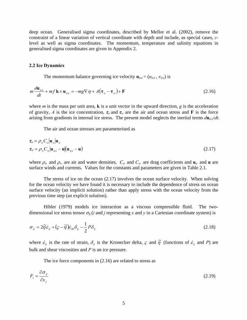

10
Ice Ridging
The function Wr representing ridging in (228) is written in terms of thickness distribution functions a(h) and n(h) as
( ) ( )( ) ( )[ ]int minus
+minus=
dhhnhahnhaghWr )( (230)
The denominator in (230) ensures that the first constraint (226) is satisfied a(h) is the distribution of ice which undergoes ridging (the source) n(h) is the distribution of the newly ridged ice (the destination) Thorndike et al (1975) suggest a(h) of the form
)()()( hghbha = (231) where b(h) selectively weights thin ice for participation in the ridging Thorndike et al (1975) suggest b(h) of the form
⎩⎨⎧
gtltleminus
=lowast
lowastlowast
GhGGhGGhG
hb)(0
)(0)(1)( (232)
where G(h) is the cumulative distribution function
( ) hdhghGh
primeprime= int0)( (233)
and lowastG is a cutoff value Ice from the thickness distribution above the cutoff does not contribute to the ridging
The destination distribution n(h) has the form of a convolution integral
( )int primeprime= dhhahhhn )()( γ (234) where )( hhprimeγ represents the ice ridged from thickness hprime to thickness h In order that the second constraint (227) is satisfied we require
int prime=prime hdhhhh )(γ (235)
We follow Thorndike et al (1975) and take )( hhprimeγ as
( ) ( )hkhk
hh primeminus=prime δγ 1 (236)
11
which states that ice ridges to a multiple k of the original thickness Note that (236) satisfies the constraint (235) An alternative form for )( hhprimeγ is suggested by Hibler (1980) Table 21 Parameters related to ice dynamics and redistribution symbol parameter value ρi reference ice density (216) 910 kg m-3
ρa reference air density (217) 13 kg m-3
ρo reference water density (217) 1035 kg m-3
Ca air-ice drag coefficient (217) 3 times 10-3
Cw ice-water drag coefficient (217) 18 times10-2
e ratio of ellipse axes (221) 2 P ice strength parameter (222) 25 times 104 Pa C parameter in ice pressure (222) 20 G cutoff for cumulative distribution function in ridging (232) 015 k ratio of thickness in ridging (236) 15 24 Ice Thermodynamics
The coupled model is forced at the surface by atmospheric variables wind air temperature dew point temperature cloudiness and precipitation We first describe the parameterisations for heat fluxes We then describe the surface heat balance and the thermodynamic coupling between ice and ocean Surface Heat Fluxes Sensible Heat The upward flux of sensible heat HS is given as
( )asaHpaas TTuccH minus= ρ (237) where ρa is the density of air cpa is the specific heat of air cH is the transfer coefficient ua is the wind speed Ts is the surface temperature (ice or ocean) and Ta is the air temperature at the standard level Over water values of cH as functions of wind speed and atmospheric stability are taken from Smith (1988) Over ice cH is constant (Table 22)
12
Latent Heat Upward latent heat flux HL is given as
( )saaEaL qquLcH minusminus= ρ (238) where L is the latent heat of vaporization or sublimation cE is the transfer coefficient qa is the specific humidity at the standard level and qs is the specific humidity at the surface Over ocean cE is taken as 15 cH where cH is from Smith (1988) Over ice cE is taken as a constant The rate of evaporation is determined from (238) as HLL
Specific humidity is related to vapour pressure e by
( )epeq
atm εε
minusminus=
1 (239)
where ε = 0622 is the ratio of molecular weight of water vapour to dry air and patm is the atmospheric pressure The specific humidity at the surface is assumed saturated Saturation vapour pressure over water ew (in mbar where 1 mbar = 102 Pa) at temperature T (oC) from the Smithsonian Meteorological Tables (cited in Gill 1982) is log10 ew (T) = (07859 + 003477 T)(1 + 000412 T) Saturation vapour pressure over ice ei (mbar) at temperature T (oC) is log10 ei (T) = log10 ew (T) + 000422 T Solar Radiation An empirical formulation for incoming short-wave radiation by Shine (1984) is used The Shine formula for Qo the short-wave radiation (W mminus2) under cloudless skies is
( ) 04550cos21101coscos5
2
++times+= minus ZeZ
ZSQo (240)
where S is the solar constant (taken as 1353 W m-2) Z the solar zenith angle and e is the vapour pressure in Pa The cosine of the zenith angle is cos Z = sinφ sinδ + cosφ cosδ cos HA where φ δ and HA are latitude declination and hour angle respectively The declination and hour angle are determined by δ = (2344 π 180) cos[(172 minus day of year) π 180)]
13
ΗΑ = [12 minus solar time (h)] π12 The total incoming short-wave radiation is found by modifying Qo for cloudiness Q = Qo (1 ndash 06 C3) (241) where C is the cloud fraction Long-wave Radiation Smith and Dobson (1984) give the net long-wave radiation QL following Budyko (1974) as
( ) ( )⎥⎦
⎤⎢⎣
⎡minus+minus⎟
⎠⎞
⎜⎝⎛ minus= asaaL TTCceTTQ 41
22132006602540 1
3σε (242)
where ε is the emissivity of the surface relative to a black body σ is the Stefan Boltzmann constant e is the vapour pressure (Pa) c1 is a latitude-dependent cloudiness factor Ta is the air temperature (K) and Ts is the surface temperature (K) Surface Heat Balance
Over open water the net heat flux H(0) is
LLS QHHH ++=)0( (243)
The heat flux H(h) conducted through ice of thickness h is H(h) = ki (T0 ndash Ts)h (244) where ki is the conductivity of ice T0 is the temperature at the bottom of ice (assumed the freezing point) and Ts is the surface temperature The flux (244) represents the zero-layer model of Semtner (1976) The heat conducted through the ice balances the net surface flux Hs + HL ndash (1 ndash 04 Io) (1 minus αi) Q ndash QL = H(h) (245) where αi is the albedo A fraction of solar radiation Io penetrates the ice surface creating brine pockets In (245) we follow Parkinson and Washington (1979) by neglecting 40 of the penetrating radiation and allowing the remaining 60 to heat the surface Io is taken as 017 (Parkinson and Washington 1979)
14
The temperature at the surface of the ice Ts adjusts so that the balance (245) is maintained (245) is solved iteratively If Ts is determined to be above the melting point then Ts is set to the melting point the fluxes are recomputed and the net heat flux melts ice at the upper surface
Snow has a major effect on albedo but snow thickness is not modelled in CECOM αi in (245) is set according to surface temperature following Hibler (1980) The albedo is 075 when the surface temperature is below freezing and 0616 when the surface temperature equals the melting point temperature (Dunlap et al 2007) The open water albedo is set to 01 Ice Ocean Fluxes
The heat flux at the ice-ocean interface FT is given by Mellor and Kantha (1989) as
( )TTCcFzTpoT minusminus= 0ρ (246)
where cp is the specific heat of seawater and T is the temperature at the uppermost model grid point The transfer coefficient
zTC is defined by
( ) TrT BzzP
uCt
z +minus= minus
lowast
01 lnκ
(247)
32
210
rT PuzbB ⎟⎠⎞
⎜⎝⎛= lowast
ν where lowastu = (τρo)12 is the surface friction velocity tr
P = 085 is the turbulent Prandtl number κ = 04 is the von Karman constant z is the vertical coordinate corresponding to T z0 is a roughness parameter (see below) ν is the molecular viscosity and Pr = 129 is the molecular Prandtl number The factor BT parameterises a molecular sublayer The empirical factor b is taken as 3 (see Mellor and Kantha 1989)
The roughness length z0 is a weighted sum of under ice and open ocean roughness lengths ln z0 = A ln z0i + (1 ndash A) ln z0o (248)
15
again following Mellor and Kantha (1989) The underice roughness length z0i is chosen as 005 m for ice thickness 3 m decreasing linearly to zero as ice thickness goes to zero The open ocean roughness length z0o is Charnockrsquos wave relation (Charnock 1955)
gu
za
oo ρ
ρ 2
0 0150 lowast= (249)
The salt flux at the ice ocean surface is given by Mellor and Kantha (1989) analogously
to (246) as
( )SSCFzSS minusminus= 0 (250)
where S0 is the salinity at the ice ocean interface S is the salinity at the uppermost grid point and
( ) SrS BzzP
uCt
z +minus= minus
lowast
01 lnκ
(251)
3221
co
S Suz
bB ⎟⎠⎞
⎜⎝⎛= lowast
ν
with Sc = ναs = 2432 the Schmidt number for salt diffusion (αs is the salt diffusivity) Ice Growth Rate
The heat balance across an infinitesimal control volume about the ice-ocean interface and atmosphere-ocean interface is
oT LWHAhAHF ρ00)0()1()( minusminus+= (252) where W0 is the mass rate of ice growth and L0 is the latent heat of fusion (252) expresses the balance that the weighted heat flux just above the interface less the heat flux just below the interface gives the latent heat of ice growth We assume that heat flux below the interface FT is uniform in a grid cell
Ice growth or melt results in a surface salt flux FS of
)()1())(( 0 PESASSAWWF IAIS minusminus+minusminus= (253) where SI is the salinity of ice and E and P are the evaporation and precipitation rates respectively The term WAI is the ice melt at the upper ice surface which is assumed to run off immediately The ice melt at the upper surface is discussed following (245)
16
There is one further constraint that is the temperature at the ice-ocean interface is at the freezing point as a function of salinity T0 = Tf (S0) (254) The freezing point relationship used here is that given in Gill (1982)
The set of equations (246) (250) (252) (253) and (254) is solved simultaneously for FT FS T0 S0 and W0 thereby determining the ice growth rate Frazil Ice
The formation of frazil ice in the model follows Mellor and Kantha (1989) A constraint on the ocean temperature is that it must remain greater than or equal to the freezing point Suppose that after solving the ocean heat and salt balances the temperature and salinity are T1 and S1 If T1 is below the freezing temperature Tf(S1) then temperature and salinity are changed to a new state T2 and S2 with the formation of frazil ice If the mass fraction of frazil ice is γ heat and salt balances give T2 = T1 + γ L0cp (255) S2 = S1 + γ (S1 ndash SI)
The solution of (255) is
( )( ) ( )[ ]Iffp
fp
STSTcLTSTc
minusminus
minus=
10
11γ (256)
if the dependence of the freezing point on salinity Tf(S) is linear The frazil ice is assumed for simplicity to consolidate immediately on the underside of ice Note that the amount of frazil ice formed is sensitive to the parameterisation of surface heat flux FT in (246) If the parameterisation of FT is an overestimate then the under-ice growth will be too small but the frazil ice growth will be too large Alternatively if the parameterisation of FT is an underestimate then the under-ice growth will be too large but the frazil ice will be too small The total ice growth is not overly sensitive to the parameterisation (246) but depends on atmospheric cooling and heat fluxes within the ocean
17
Table 22 Constants and parameters for thermodynamics Symbol Parameter Value cpa specific heat of air (237) 1005 J kg-1 Kminus1
cH sensible heat transfer coefficient over ice (237) 175 times 10-3
L latent heat of vaporisation (238) 25 times 106 J kg-1
L latent heat of sublimation (238) 28 times 106 J kg-1
cE latent heat transfer coefficient over ice (238) 21 times 10-3
ε emissivity (242) 095 σ Stefan Boltzmann constant (242) 567 times 10-8 W m-2 K-4
αw albedo water (27) 01 ki ice conductivity (244) 204 W m-1 deg C-1
αi albedo ice (245) 0616 αι albedo snow (245) 075 cp specific heat of seawater (246) 399 times 103 J kg-1 deg C-1
ν seawater kinematic viscosity (247) 18 times 10-6 m2 s-1
SI salinity of ice (253) 5 L0 latent heat of fusion (253) 332 times 105 J kg-1
3 Finite Difference Implementation 31 POM
The equations governing the ocean dynamics support the propagation of fast moving external gravity waves and slow moving internal waves A mode splitting technique is used to separate the vertically-averaged velocity (external mode) from the vertically-varying velocity (internal mode) For the external mode the depth-integrated continuity equation (A22) and depth-integrated momentum equations (A23) and (A24) use a short time step with terms involving depth-varying velocity fixed The external model provides sea level elevation η and depth-averaged velocity kus kvs so that internal mode equations can be integrated with a much longer time step
POM employs a C grid in the horizontal It is implemented on an orthogonal curvilinear
coordinate system which includes Cartesian coordinates and spherical coordinates as special cases Generalised sigma coordinates are used in the vertical
For open ocean boundary conditions we use the flow relaxation scheme (FRS) of
Martinsen and Engedahl (1987) which has been applied by Slordal et al (1994) The FRS boundary conditions require a relaxation zone along each open boundary At the exterior of the FRS zone we specify a solution φext For each time step we calculate a solution φint in the interior from the model equations We then obtain the solution φ in the FRS zone by relaxation φ = αφext + (1 minus α)φint (31)
18
The relaxation parameter α is 1 at the exterior of the FRS zone and varies smoothly towards 0 at the interior boundary of the zone Here we choose α as α = 1 ndash tanh(2xE LE) (32) where LE is the width of the FRS zone xE = 0 at the exterior boundary and xE = LE at the interior boundary We choose LE as five grid intervals
We apply the FRS boundary conditions to sea level elevation the horizontal components of velocity temperature and salinity We specify values of vertical velocity and turbulence quantities at FRS exterior boundaries but do not relax these quantities 32 Ice Dynamics The spatial finite difference grid for the ice model defines ice velocity at grid cell vertices and ice concentration at the grid cell centers The finite difference procedures for solving the momentum balance the ice stress terms and the ice advection equation (including the diffusion terms) are described by Hibler (1979) The point relaxation solution for the internal ice stress of Hibler has been replaced by a more efficient line relaxation scheme devised by Zhang and Hibler (1997) A spherical coordinate system is used the governing equations are given in Zhang and Hibler (1997) 33 Mechanical Redistribution of Ice Thickness Distribution Function
The finite difference thickness distribution discussed in this section and the discrete redistribution function and ridging function discussed in subsequent sections follow Flato (1994) In finite difference form we define M discrete ice categories In Figure 31 we show the thickness categories and the other discrete variables The thickness boundaries are h0 h1 helliphM In general the thickness intervals are unequal The centers of the thickness intervals are given by
cM
cc hhh 21 K ch1 is defined as 0 and the first thickness category represents open water The discrete thickness distribution is defined
intminus
= i
i
h
hi dhhgg1
)( i = 1hellipM (33)
gi is the fraction of area occupied by the ith thickness category The cumulative thickness distribution is
⎪⎩
⎪⎨⎧
==
= sum =1
00
1Mig
iG i
j ji K
(34)
19
(The subscript notation here differs from Flato 1994) The ice volume per unit area (mean ice thickness) corresponding to (224) is
i
M
i
ci ghh sum
=
=1
(35)
The change in the discrete thickness distribution (corresponding to (225)) is
diffusionFFgt
giiiiice
i +Ψ+minus=sdotnabla+part
partminus1)(u
(36)
iΨ is the discrete mechanical redistribution function (discussed next) Fi is a flux of ice from one category to the next from growth or melt (discussed in Section 34)
Figure 31 Schematic diagram showing the thickness boundaries and locations at which the discrete variables are defined Redistribution Function
The discrete redistribution function iΨ for Hiblerrsquos (1979) plastic rheology is defined from (229) as
( ) ( )( )⎪
⎩
⎪⎨
⎧
=minusΔ
=minusΔ++Δ=Ψ
MiW
iW
jjri
jjrijj
i
Kamp
ampamp
221
121
21
ε
εε (37)
where Wri is the discrete ridging function
20
Ridging Function
The discrete participation function bi (corresponding to (232)) is defined at thickness boundaries
lowastminus=GG
b ii 1 i = 0hellipM (38)
The discrete distribution function ai governing the ice which contributes to ridging (corresponding to (231)) is
( )
⎪⎪⎪
⎩
⎪⎪⎪
⎨
⎧
gt
gtgtminusminus
ge+
=
minus
minusminus
minuslowast
minus
minus
1
11
11
1
00
0)(2
02
i
iiii
iii
iii
i
i
b
bbhhhhbg
bbbg
a (39)
where h is interpolated as
11
11 minus
minus
minusminus
lowast
minusminus
+= iii
iii b
bbhh
hh (310)
ai is defined for i = 1 hellip M
The discrete distribution function ni governing the thickness into which the ridging
occurs [corresponding to (234)] is
sum=
=M
jjjii an
1γ i = 1hellipM (311)
The function γji transfers ice from the jth category to the ith category Before normalisation it can be written
⎩⎨⎧ ltle
= minus
otherwise01 ˆ 1 i
cji
jihkhhk
γ j =1hellipM i = 1hellipM minus 1
When i = M the criterion for jiγ to be nonzero is modified to c
jM khh leminus1 ie ice which would otherwise ridge into a thickness greater than the upper limit is placed into the maximum ice thickness category The transfer function is normalised to satisfy (236)
21
sum=
l jlcl
cj
jiji hh
γγγ
ˆˆ i j = 1hellipM (313)
The discrete ridging function (corresponding to (230)) may now be written
( )sum =minus
+minus= M
j jj
iiri
na
naW
1
(314)
and substituted into the redistribution function (37)
34 Thermodynamic Redistribution of Ice
The implementation of the discrete thermodynamic redistribution described in this
section follows Hibler (1980) Heat budgets (243) to (245) are solved at the water surface and the surface of ice for each ice category and determine the heat flux through ice The ice growth rates fi at c
ih in the ice distribution equation (225) are determined from the heat fluxes and the ocean heat balance according to (252)
The flux of ice between categories Fi in (36) is defined from the ice growth rates by an
upstream difference
( ) )0min(0max
1
11ci
ci
iiiii hh
gfgfFminus
+=
+
++ (315)
The fluxes must satisfy two constraints The first is that the flux of ice between
categories does not change the total area of ice The second is that the change in ice volume must equal the ice grown or melted With M ice categories the rate of change in ice area per unit area expressed in terms of fluxes is
( )sum=
minus minusM
iii FF
11 (316)
The change is zero provided that F0 = FM = 0 Considering the second constraint the rate of change of volume of ice grown or melted per unit area is
sum=
M
iii gf
1 (317)
Expressed in terms of the fluxes the rate of change in ice volume is
22
( )sum=
minus minusM
i
ciii hFF
11
( )summinus
=+ minus=
1
11
M
i
ci
cii hhF
( ) ( )[ ]summinus
=+++=
1
111 )0min0max
M
iiiii gfgf (318)
( ) ( )summinus
=
++=1
20min0max
M
iMMiiii gfgfgf
(317) and (318) are equal except in the case of f1 negative (open water is absorbing heat) and the case of fM positive (ice from the thickest category is growing) The fluxes Fi in (315) must then be modified to account for these two cases in addition to the requirements following (316)
Open Water Absorbing Heat
In the case of open water absorbing heat we specify that the heat is mixed under the ice and contributes to melt at the bottom surface of the ice We modify the rates of change of ice thickness to if prime
( )⎩⎨⎧
gtminus+=
=prime1110
1 iAfAfi
fi
i (319)
where A is the total ice concentration Note that (319) preserves the net rate of ice growth
sumsum==
=primeM
iiii
M
ii gfgf
11 (320)
Growth of Thickest Ice Category
The second case in which flux of the form (315) does not balance the change in ice volume is when the thickest ice is growing In this case we add thick ice growth proportionally to all ice categories Let
hgfC MM=1 (321)
Then define the flux
23
⎩⎨⎧
gt=minus
=1
1
1
1 igC
iACF
iithick (322)
The flux (322) has the property that the increase of ice area is balanced by a decrease in
open water area Note also that the total rate of increase in ice volume from Fthicki balances the rate of increase of volume from growth of the thickest ice category ie
MMci
M
iithick gfhF =sum
=2 (323)
Maximum Rate of Decay
Hibler (1980) suggests applying a maximum rate of ice decay (minimum growth rate) fmin taken here as minus015 m day-1 We modify the ice growth rates
( ) iimini gfff prime=primeprime max (324)
The difference between ii ff primeprimeprimeand represents excess heat which melts ice laterally The excess rate of decay is
( ) i
M
iii gffExcess sum
=
primeminusprimeprime=1
(325)
Similarly to the thick ice growth we allocate this decay proportionately to all ice categories Define
hExcessC =2 (326)
then the lateral melt in terms of a flux is
⎩⎨⎧
gtminus=
=1
1
2
2 igC
iACF
iilateral (327)
The redistribution of ice from growth or melt can be finally written as
ithickilateraliii FFFF
tg
1 ++minus=Δ
Δminus (328)
24
4 Canadian East Coast Ocean Model (CECOM)
The region of interest for the model extends from the Gulf of Maine in the south to Baffin Bay in the north The model is implemented on a spherical coordinate system To reduce the impact of converging meridians we select a spherical coordinate system that is rotated relative to the earthrsquos longitude and latitude so that the equator of the rotated system bisects the domain In the following sub-sections the coordinate transformation and model domain are described
41 Rotated Spherical Coordinates
The relation between Cartesian coordinates (x y z) and longitude and colatitude (φ θ) (refer to Figure 41) is x = sinθ cosφ y = sinθ sinφ (41) z = cosθ where we take the radius of the sphere as unity Consider the transformation from original coordinates r to coordinates in a rotated system rprime
⎟⎟⎟
⎠
⎞
⎜⎜⎜
⎝
⎛=
zyx
r rArr ⎟⎟⎟
⎠
⎞
⎜⎜⎜
⎝
⎛
primeprime=prime
zyx
r (42)
A rotated system can be defined by the successive application of three rotations (Figure 42) 1 angle ξ about the z axis 2 angle η about the new y axis and 3 angle ζ about the new z axis The angle of rotation is in the clockwise direction looking in the direction of the axis The transformations from r to rprime and components of vectors are given in Appendix 2
25
Figure 41 Spherical coordinate system with longitude φ and co-latitude θ
Figure 42 The decomposition of a coordinate system rotation into three successive rotations of ξ η and ζ The red line is the y axis after one rotation 42 The CECOM Domain
The CECOM model grid has a resolution of 01deg times 01deg As noted it is defined on a rotated spherical coordinate system (Figure 43) The model domain in the geography
26
coordinates and the inner and outer boundaries are shown in Figure 44 The bathymetry of the domain is drawn in Figure 45 Specifics of the domain are given in Table 41
Generalised sigma coordinates are used to retain near-surface resolution even as bottom
depth increases The procedure we use to select the vertical levels is somewhat arbitrary For sufficiently deep water (bottom depth greater than or equal to H1) we specify that a fixed upper layer and the underlying ocean each have a given number of levels The levels are scaled according to the fixed upper or varying lower layer thickness For shallow water (bottom depth less than or equal to H0) all levels are distributed uniformly Between H0 and H1 the levels are linearly interpolated between the levels for H0 and H1
H0 = 10 m H1 = 64 m and an upper layer thickness of 64 m are selected There are a
total of 21 levels with 8 levels in the upper layer and 13 levels in the underlying ocean (at depths greater than H1) These generalised coordinates are shown for a section across the Labrador shelf (27deg longitude in rotated coordinates) in Figure 46
Figure 43 CECOM grid defined by a rotated spherical coordinate system Lines of longitude and latitude in the rotated system are drawn in red
27
Figure 44 CECOM domain (green) in the geographic coordinates The double red lines are the inner and outer boundaries of the model The blue box is the boundary in the rotated system of Fig 43
28
Table 41 Specifications of the CECOM domain ________________________________________________________________________ Coordinate rotation ( ) )1718241( degminusdegdeg=ςηξ Extent (rotated coordinates) 0 to 40deg longitude minus11 to 103deg latitude Horizontal resolution 01deg times 01deg
Dimension 400 times 213 times 21 (east times north times vertical) 410 times 223 times 21 including boundary relaxation zones time step 450 s (internal) 15 s (external) ________________________________________________________________________
Figure 45 The bathymetry of the CECOM domain Depth contours of 200 1000 2000 hellip m are drawn Specified transports (Sv) at open ocean boundary are indicated
29
Figure 46 A cross-section of the generalized coordinates across the Labrador Shelf The upper panel shows the coordinates over the upper 200 m 43 Ocean Initial State Boundary Conditions and Model Spin-up
Monthly climatological ocean temperature and salinity are used as an initial state and as open ocean boundary conditions The monthly climatologies were obtained from an objective analysis of historical data archived at Bedford Institute of Oceanography (Tang 2007) The database covers an area from northern Baffin Bay to Cape Hatteras and from the coast to 42deg W It is derived from a variety of sources dating back to 1910 The objective analysis employed an iterative difference correction procedure with topography-dependent radii of influence The grid resolution is 16deg times 16deg Figure 47 is a sample plot from the data set showing surface temperature and salinity for September
30
Figure 47 Surface temperature and salinity for September from objective analysis The red dots are the locations of the raw data
31
Transports based on large-scale models and observations are specified at the open boundaries of the model (Clarke1983 Ezer and Mellor 1994) In the present implementation the transports as shown in Figure 45 are used Different specifications are being tested to obtain best results The vertical profile of normal velocity is determined by the density through the geostrophic relation The sea level elevation at the open boundaries is determined by geostrophy to within a constant
The model open ocean boundary (double red lines in Fig 44) is interrupted by land masses The procedure to determine sea level in the ocean straits (Nares Strait Lancaster Sound Jones Sound Hudson Strait and St Lawrence Estuary) is as follows We spin up the model with three diagnostic runs of 10 days duration each with zero wind stress The sea level at open boundaries of straits is set to the adjacent interior value from the end of the previous run The spin-up concludes with a 10-day prognostic run
The initial state consists of September temperature and salinity and zero ice We create
12 open ocean boundary conditions corresponding to the monthly temperature and salinity fields As noted previously the geostrophic relation determines sea level elevation only to within a constant The constants ie the sea level average across open boundaries in straits are determined from the spin-up The monthly boundary conditions are linearly interpolated to daily values The sea level elevation and transport stream function after the spin-up process are drawn in Figure 48
Figure 48 The sea level elevation (left) and transport stream function (right) following the spin-up process
32
44 Ice categories
The ice model is implemented with 10 ice thickness categories with boundaries at 005 018 038 066 106 158 224 304 398 and 504 m The corresponding central thicknesses c
ih are 0 012 028 052 086 132 191 254 351 and 451 m 5 Model Physics of WaveWatch III (WW3)
The WAVEWATCH III (hereafter WW3) wave model (version 222) is used in the BIO forecasting system to forecast wave height and direction This is a WAM-type ocean surface wave model developed at NOAANCEP (Tolman and Chalikov1996 Tolman 2002) It has been successfully applied in global and regional scale studies in many areas including the North Atlantic and has proven to be an effective tool to study wave spectral evaluation air-sea interactions and nonlinear wave-wave interactions WW3 is a discrete spectra and phase-averaged model (Battjes 1994)
For regional and global applications the directional wave spectrum is resolved at each model grid point in terms of wavenumber-direction bands and the evolution of the wave field is found by numerically solving the spectral wave action balance equation which is usually written as
σθ
θλ
λθφ
φφSNNk
kNN
tN
g =partpart
+partpart
+partpart
+partpart
+partpart ampampampamp cos
cos1 (5-1)
where λ is longitude φ is latitude θ is wave propagation direction k is wave number t is time σ is the intrinsic angular frequency WW3 evaluates the balance equation for the wave action spectrum )( txkN θ which is usually expressed in spherical coordinates (Komen et al 1994)
The derivatives in (5-1) are the propagation velocities in physical and spectral domains
RUcg φθ
φ+
=cosamp
φθ
λ λ
cossinR
Ucg +=amp
Rcg
g
θφθθ
costanminus= ampamp R is the radius of the earth and
φU and λU are current components in φ and λ directions The left side of equation (1) represents the local rate of change of wave action density propagation in physical space action density shifting in frequency and direction due to the spatial and temporal variation in depth and current The net source term S consists of wind input( inS )white-capping dissipation( dsS ) nonlinear wave-wave interactions( nlS ) and bottom friction( botS ) WW3 uses an explicit scheme to solve the action balance equation (1) for N
Two combinations of the source terms inS and dsS are available in WW3 The default set up of WW3 corresponds to the wave-boundary layer formulation for inS and dsS due to Tolman and Chalikov (1996) Tolman (2002) notes that application of this formulation has entailed a
33
correction in fetch-limited wave heights that results from atmospheric stratification which necessitates a re-tuning of the model by defining an lsquoeffectiversquo wind as well as an additional correction for the impact of stability on wave growth An alternate combination corresponds to WAM cycle 3 physics (hereafter denoted WAMC3 physics) in which inS and dsS are based on WAMDI (1988) Snyder et al (1981) and Komen et al (1994) Quadruplet nonlinear interactions nlS are simulated by DIA and bottom dissipation bfS by the JONSWAP parameterization of Hasselmann et al (1973) Padilla-Hernatildendez et al [2007] compared the WW3 model against WAM and SWAN models for two North Atlantic storms and found that WW3 provided the high quality statistical comparisons to deep water observations 6 The Bedford Institute Ocean Forecasting System (BIOFS) BIOFS is a real-time short-term (2-day) forecasting system for eastern Canadian waters The forecast period is constrained by input data from Environment Canada If meteorological data from long range weather forecasts are available the ocean forecasts can be extended to a longer period It consists of two sub-systems one for CECOM (Section 63) and one for WW3 (Section 64) Graphic display of the forecasts can be viewed at the following public website maintained by DFO httpwwwmardfo-mpogccascienceoceanicemodelice_ocean_forecasthtml The parameters displayed on the website are surface trajectories water level time series at selected locations ice concentration and thickness wave height and direction (Northwest Atlantic and Atlantic Maritimes) sea surface elevation (non-tidal) maps temperature at surface and 50 m They are given at hourly (water level time series) 6-hourly (wave) or 12-hourly (all others) intervals 61 Input Data Meteorological Data Meteorological forcing is taken from the Canadian Meteorological Centre (CMC) Global Environmental Multiscale (GEM) model (Mailhot et al 2006) which provides 48 hour forecasts twice daily at 0000 and 1200 UTC with fields output at 3 hour intervals The GEM model is an operational atmospheric model that is part of the Canadian Regional Forecast System (RFS) developed by Environment Canada The model uses a variable resolution grid over the entire globe with a mesoscale 15 km horizontal resolution window over Northern America Fields used in the forecasting system are 10m winds 2m air and dew point temperatures total cloud coverage and total accumulated precipitation All meteorological parameters are linearly interpolated to the ocean and wave model grids Except for the10 m winds the parameter values change every 3 hours For CECOM the 10m wind field is interpolated in time to the model time step of 75 minutes to avoid temporal discontinuities in the dynamical forcing Total accumulated
34
precipitation is converted to a precipitation rate For WW3 the wind fields are interpolated to the propagation time step of the respective wave model (see Section 64 for details) Sea-Ice Data Ice concentration data are used for data assimilation (Section 62) in the ice model and to define the wave domain in WW3 In WW3 a grid point is considered open ocean if the ice concentration is equal or less than 05 Otherwise it is considered land Digital sea ice charts which include ice concentration data are provided by Canadian Ice Services(CIS) Canadian waters are covered by five digital ice charts (Figure 61) Data from Eastern Arctic Hudson Bay and East Coast are used in the forecasting system CIS produces daily charts for the Gulf of StLawrence and the Labrador and Newfoundland coasts south of 58N Regional charts for Hudson Bay Baffin Bay and the Labrador coast north of 58N are produced fortnightly Typically the regional charts are released several days after the date for which they are valid Since these charts represent more of a two week average condition than an instantaneous one BIOFS uses a regional charts release date as its valid date
Figure 61 Coverage of CISrsquos digital ice charts (courtesy of CIS) The digital charts use the ldquoegg coderdquo (Environment Canada 2005) to indicate the sea ice partial concentration for each stage of development on a regularly spaced grid Each ldquoeggrdquo indicates up to three different ice types (ignoring trace amounts) each of which is assigned a stage and concentration The stage of development may be interpreted as an approximate
35
measure of the ice thickness The conversion of stage to ice model thickness category is illustrated in Table 61 There are also four special cases listed in Table 62 Table 61 Conversion from ice stage to ice model category
Ice stage of development Description
Ice model
categoryIce thickness
boundaries (m)
OW BW IF Open Water bergy water ice-free 1 -005 lt h le 005
1 New 2 005 lt h le 018
2 Nilas 2 005 lt h le 018
3 Young Unknown 3 018 lt h le 038
4 Young Grey 2 005 lt h le 018
5 Young Grey-White 3 018 lt h le 038
6 First Year Unknown 4 038 lt h le 066
7 First Year Thin 5 066 lt h le 106
8 First Year Thin First Stage 5 066 lt h le 106
9 First Year Thin Second Stage 5 066 lt h le 106
1 First Year Medium 6 106 lt h le 158
4 First Year Thick 7 158 lt h le 224
7 Old 8 224 lt h le 304
8 Old Second Year 9 304 lt h le 398
9 Old Multi-Year 9 304 lt h le 398
L Ice of Land Origin 9 304 lt h le 398
B Brash 3 018 lt h le 038
Each stage of development is first converted to a category The partial concentrations
and categories including flags (Table 62) are then nearest-neighbour interpolated to the model grid Grid points with land fast ice will be filled with neighbouring concentrations and categories Including flags in the interpolation preserves grid points which should not be filled by interpolation All the charts available for a forecast date are then combined Where charts overlap the concentrations of each category are averaged Flagged points are ignored in the averaging
36
Table 62 Interpolation of ice data
Ice stage of
development Description Action
POINT NOT COVERED BY
POLYGON Point is outside CIS analysis area Flag
LAND Land point Flag
ICEGLACE Useless CIS category indicating ice presence but not providing concentration or stage
Flag
FASTICE Land fast ice Nearest Neighbour
Tides Tidal constituents of elevation and velocity come from two sources Paturi et al (2008) provides eight constituents (M2 S2 N2 K2 K1 O1 P1 Q1) and covers most of the model domain up to Davis Strait Dunphy et al (2005) provides five tidal constituents (M2 S2 N2 K1 O1) for Baffin Bay Constituents are linearly interpolated to the model grid Where the two sources slightly overlap at Davis Strait matching constituents are averaged 62 Data assimilation in CECOM
Many assimilation schemes have been developed for oceanographic and meteorological applications in the past 20 years Advanced schemes such as 3-d and 4-d variational method and Karmen filter require massive resources and abundant data to yield optimum results In this section we describe three methods to assimilate the annual cycle of the temperature and salinity fields sea surface temperature and ice concentration data into the ocean forecast model Assimilation of the Annual Cycle of the Temperature and Salinity Fields Monthly temperature and salinity climatologies are prescribed at the open boundaries of CECOM Such constraints are not strong enough to prevent the temperature and salinity fields from drifting in multi-year integration To ensure the annual cycles are preserved a nudging term with a constant relaxation time scale tR of 45 days are added to the temperature and salinity equation
37
)(1 TTtt
TCLIM
R
minus+=partpart
)(1 SStt
SCLIM
R
minus+=partpart
where TCLIM and SCLIM are monthly temperature and salinity climatologies linearly interpolated to daily intervals Assimilation of Sea Surface Temperature Data Daily near real-time sea surface temperature (SST) derived mainly from satellite observations are provided by CMC The data are assimilated into the ocean forecast model using a flux correction method The method is based on the theory of optimal interpolation A correction term proportional to the differences between the modeled and observed SST is added to the heat flux equation
We first consider the equation for SST assimilation (see Appendix 4)
( ) [ ])()(
2exp)()( 2
2
22
2
om
ooo
om
mma tTtTtt
tTtT minus⎥⎥⎦
⎤
⎢⎢⎣
⎡ minusminus
++=
τεεε
(61)
where the superscripts and subscripts ldquoardquo ldquomrdquo and ldquoordquo in (61) denote ldquoassimilationrdquo ldquomodelrdquo and ldquoobservationrdquo respectively to is the time of the most recent observation and t is the model time 2
mε and 2oε are the model and data errors respectively τ is the correlation time scale of
SST Since change in SST ΔT is related to change in heat flux ΔQ by
Qhc
tT
p
d Δ=Δρ
where h is the mixed layer depth and td is the time interval of SST data the first terms on each side of (61) can be replaced by the corresponding heat fluxes The equation for SST data assimilation is
( ) [ ])()(2
exp)()( 2
2
om
ooo
d
pma tTtTtt
Ft
hctQtQ minus
⎥⎥⎦
⎤
⎢⎢⎣
⎡ minusminus+=
τρ
(62)
where F = 1 [1+ (εο εm)2] F ranges from 0 to 1 Not all parameters in (62) are well known To implement (62) in the forecast model the parameters are adjusted to yield optimal results
38
Figures 62 and 63 show the impact of data assimilation on model SST from a test run In this run F = 1 td = 1 day τ = 1 day were used and h = 20 m To reduce model noise in the run )( o
m tT in (62) was replaced by the model SST averaged over the previous day (from t0 - 1 day to t0) Significant improvements in the model SST can be achieved by using this assimilation scheme Without data assimilation the difference between the model and data at the Scotian Shelf is of the order of ~ 2o C The difference is reduced to a fraction of a degree with data assimilation Over the model domain the model without data assimilation over predicts SST in the northern Labrador Sea and under predicts SST in the coastal and the North Atlantic Current regions (Figs 63) Data assimilation is able to reduce the errors to less than 1o C
The SST assimilation is applied to ice free waters only In ice covered areas the sea
surface temperature is equal or very close to the freezing temperature
Figure 62 A comparison of SST in a 1o x 1o area centered at the indicated location with and without data assimilation
39
Figure 63 CMC SST (left) and the difference between the model and data with (middle) and without (right) data assimilation Assimilation of sea-ice data An insertion-nudging method is used for ice data assimilation Ice concentration data are inserted to the model gradually and the model concentration is restored to the data value with a prescribed time constant In the equation for the thickness distribution function a term proportional to the difference between the observed and values is introduced
( ) ( ))( ioi
iiice
i ggdiffusionhfg
gt
gminusΓ++Ψ=
partpart
+sdotnabla+part
partu (62)
where goi is the ice chart concentrations and gi is the model concentrations for ice of thickness category i Γ has the following form
⎥⎦
⎤⎢⎣
⎡ minusminus=Γ 2
2
2)(
expw
om
ttγ
γ (63)
where t is the model time to is the time for which the ice chart is valid γm and γw are adjustable parameters The Gaussian function in (63) limits nudging to the times around the ice chart time 1γm is the restoring time scale In the present implementation the values of 1γm and γw are set to 16 hours (5760 seconds) and 3 hours (10800 seconds) respectively At one hour from the ice chart time this scheme gives a concentration change rate of ~05 per hour At times plusmn 2γw from
40
the ice chart time the rate is negligible Where there is no ice chart data the nudging is not applied Figure 64 is a comparison of ice area south of 58o with and without data assimilation for January 2008 Figure 65 shows the ice concentration from CISrsquos East Coast ice chart and the model results with and without data assimilation The data assimilation significantly reduces the model error In particular ice cover in the Gulf of St Lawrence and the location of the eastern ice edge can be simulated more realistically with data assimilation
Figure 64 A comparison of the model ice area south of 58o N with (blue) and without (black) data assimilation The unit is percentage of the model area south of 58o N
41
Figure 65 Ice concentration for January 28 2008 data (left) model results without (middle) and with (right) data assimilation 63 Operational Implementation of CECOM The ice-ocean component of BIOFS is mostly comprised of MATLAB scripts that handle the pre-processing of model input fields the execution of the CECOM FORTRAN executable the post-processing of model results and the management of data files MATLAB was chosen for its platform independence interpolation and graphics functionalities and the abundance of open source tools such as M_Map (Pawlowicz 2006) readgrib (Blanton 2005) snctools (Evans 2007) and T_Tide (Pawlowicz et al 2002) Scheduling and automation is handled by the Linux bash shell but could easily be implemented for other platforms and operating systems Delivery of Meteorological and ice Data
As with any endeavor in real-time forecasting the primary concern is the timely delivery of the data required to force the forecast model To address this concern a separate subsystem written in bash shell scripts automates the retrieval of crucial meteorological forecast data transmitted from CMC to BIO server Emerald2 twice a day The subsystem polls the site for data and performs file checks after retrieval to verify file integrity There is usually a 5-6 hour delay between the CMC regional forecast and the appearance of the forecast data on their ftp site If the system fails to retrieve the data it retries for a predefined number of times The digital ice charts valid for 1800 UTC are delivered daily to an ftp server at BIO Starfish at ~2200 UTC The CIS delivery system itself checks for file integrity after delivery
42
Forecast Schedule CECOM is run three times daily within BIOFS producing 48 hour forecasts for 0000 and 1200 UTC (Table 63 Fig 66) Due to delays in receiving the meteorological data the CMC 1200 UTC data are received at ~1700-1800 UTC and the forecast completes at ~1800-1900 UTC A 1200 UTC data assimilation run using 1800 UTC sea ice concentration data and 1200 UTC sea surface temperature data (the same SST are received in the CMC 0000 UTC forecast data) is made the following morning at ~0300 UTC to assimilate the most recent ice chart and sea surface temperature data The 0000 UTC forecast is run four hours following the data assimilation run at ~0700 UTC Table 63 Ocean forecast schedule Both the local time ldquoATrdquo (Atlantic Time) and UTC are indicated
Day 1 Day 2
1 ndash 2 pm AT 2 ndash 3 pm AT 6 pm AT 11 pm AT 1 ndash 2 am AT 3 am AT
1700-1800 UTC 1800-1900 UTC 2200 UTC 0300 UTC 0500-0600 UTC 0700 UTC
CMC 1200 UTC forecast data
received
1200 UTC 48-hour forecast
CIS charts received
1200 UTC 48-hour ice
and SST assimilation
CMC 0000 UTC forecast data received
0000 UTC 48-hour forecast
43
Figure 66 Flow chart of the forecasting operations in a 24-hour period Forecast Methodology Each forecast is initialized with the most recent output of a previous forecast The ocean lateral boundary conditions are linearly interpolated to daily values from the monthly means to prevent discontinuity The boundary conditions also provide a constraint for temperature and salinity near the boundaries In the interior nudging and statistical interpolation are used to prevent long-term drifts and to assimilate sea surface temperature data into the model (see Section 62)
CMC 1200UTC data
CIS 1800UTC data
CMC 0000UTC data
12 UTC
forecast run
Data assim
ilation run
00 UTC
forecast run
1200 UTC forecasts
0000 UTC forecasts
Day 1 Day 2 Day 3
Ice concentration data
Sea surface temperature data
Add tide and Stokes drift
Add tide and Stokes drift
44
After the model run T_Tide (RPawlowicz et al 2002) calculates the tidal current and
elevation for the forecast period The tidal components are then linearly added to the forecast components For surface currents wave induced Stokes drifts are added to the model surface current to obtain the total surface current (Tang et al 2007) The Stokes drift us is obtained from the 2-dimensional wave spectrum E (f θ) of WW3 by integrations over frequency and direction
( )intint= θθπ dfdfEef kz
s 4 2ku (64)
where f is wave frequency θ is wave direction k is wave number and k is the magnitude of k
There are two options for the Strokes drift in the forecasting system us can be computed directly from (64) at every model grid point A simpler method is to parameterize us by surface winds us = a W + b W2 (65)
β = turning angle (positive for clockwise) relative to wind direction (66) where us and β are the magnitude and direction of us respectively and W is 10 m wind speed The parameters a b and β are determined from least-squared fits of the Strokes velocities computed from (64) for October-December 2007 In most applications (eg surface drifter floating object) vertically averaged surface currents are required The Stokes velocities in (65) and (66) are replaced vertically averaged Stokes velocities The results of the least-squared fits are given in Table 64 for different depths of averaging Table 64 Parameters values of the Stokes drift for different depths of averaging Depth (m) 1000a 1000b β (deg)
1 2525 0641 380 2 1656 0533 400 3 1176 0459 410 4 0889 0405 430 5 0699 0363 440
Drift tracks are calculated from the total surface current field Each track starts at a model grid point and is advected by the surface current Horizontal linear interpolation is used to calculate the surface current field between grid points Distances are calculated using the plane sailing method which ignores the earths curvature
45
For ice forecasts all available 1800 UTC ice charts from the previous day are processed and assimilated into the model to correct the model ice field as described in Section 62 For ocean forecasts 1200 UTC SST data from the previous day are assimilated into the model (Figure 66) 64 Operational Implementation of WW3
The wave models are implemented on a system of three nested grids (Figures 67 68 69 and Table 65) The spatial resolution increases from 10o in the coarse grid to 05o in the intermediate grid to 01667o (10rsquo) in the fine resolution grid This system of grids ensures that energy from distant storms is not lost in simulating storms making landfall in coastal areas of North America The grid dimensions and resolutions are given in Table 65 Etopo2 bathymetry is used from the United States National Geophysical Data Center at 2 minutes resolution WW3 is used for the coarse intermediate and fine resolution simulations Following the Courant-Friedrichs-Leacutevy (CFL) stability criterion the propagation time steps for WW3 are 20 and 10 minutes for the coarse and intermediate grids respectively and 4 minute propagation steps for the fine-resolution grid In Table 65 WW3 has 4 time steps Δtg is the global time step by which the entire wave model solution is propagated forward in time Δtρ1 is the maximum spatial (xy) propagation time step for the lowest frequency which is required to satisfy the CFL criterion Δtis is the maximum intra-spectral (k θ) propagation time step which is also required to satisfy the CFL criterion and Δtst is the minimum time step for the integration of the source terms which is dynamically adjusted for each grid and for Δtg
WW3 interpolates the wind fields to the propagation time step of the respective wave model For fast moving storms WW3 has a built-in scheme to reduce the source term integration time step when the situation is changing rapidly Moreover in WW3 the source term integration time step can be set by the user Thus we set the minimum source term time step to 5 minutes in the coarse-resolution grid to adequately simulate the storms considered here For the intermediate and fine grids source term time steps were both set to 25 (see Table 65) Details regarding the spectral range and resolution of the WW3 model are given in Table 66 in terms of the lowest and highest frequencies ( lowf and highf ) number of points ( n ) frequency resolution ( fΔ ) and angular resolutions ( θΔ ) The 48-hour WW3 wave forecasts run twice daily (0000 UTC and 1200UTC) WW3 simulates waves outside nearshore areas where shallow water wave processes are not important The model includes standard physics for wave propagation growth by wind nonlinear interactions dissipation due to whitecapping and dissipation due to bottom friction In coastal estuary and nearshore areas where water depth is shallow fine-resolution computational domains are sometimes needed for dedicated studies nested within coarserndashresolution basin-scale domains in order to resolve complex topography coastline features and shallow water wave physics In these special cases an option is that the shallow water SWAN wave model (version 4031) can be applied for a fourth domain nested within the third domain (Ris et al 1994 Booij et al 1996 Booij et al 1999 Holthuijsen et al 2003 Booij 2004) in these specific areas The physics of SWAN are different from that of WW3 especially for shallow water waves
46
SWAN can simulate shoaling refraction bottom friction and depth-induced wave breaking besides the processes for whitecapping wind input and nonlinear wave-wave interactions that are present in WW3 SWAN is formulated in terms of an action balance equation Xu et al (2007) describe the implementation of WW3 and nested grids for the North Atlantic and SWAN for Lunenburg Bay for studies related to the waves generated by hurricane Juan (September 28-29 2003)
Figure 67 Model domain of WW3 - Atlantic Ocean and sample model output (0600 UTC November 4 2007) The colors indicate significant wave height The arrows indicate wave period and direction
47
Figure 68 Model domain of WW3 ndash Northwestern North Atlantic Ocean and sample model output (0600 UTC November 4 2007) The colors indicate significant wave height The arrows indicate wave period and direction
48
Figure 69 Model domain of WW3 ndash Atlantic maritimes and sample model output (0600 UTC November 4 2007) The colors indicate significant wave height The arrows indicate wave period and direction
49
Table 65 Geographical location of the grids used in this study λ θΔ are the resolutions in longitude λ and latitudeφ and Nλ and Nφ are the number of points in λ and φ Finally tΔ is the propagation time step and tΔ ST is the required time step for source term integration for the three models as required to satisfy the CFL criterion GRIDS Longitude Latitude λ θΔ Nλ Nφ Δtg tΔ ST
Coarse 40oE ndash 82oW 75oSndash 77oN 1o 123 153 20 min 50 min
Intermediate 40oWndash75oW 20oN-75oN 05o 71 111 10 min 2min
Fine 47oWndash71oW 42oN-52oN 10rsquo 145 61 5 min 25 min
Table 66 Spectral domains for all models lowf highf are the default values
Parameters Value
lowf highf [s-1] 00418 06028
nf fΔ 29 11 ftimes
θn θΔ 36 10o
50
References Battjes JA 1994 Shallow water wave modelling Proc Int Symp Waves -Phys Numerical
Modelling University of British Columbia Vancouver I 1-23 Budyko MI 1974 Climate and Life Academic Press New York 508 pp Blanton B 2005 readgrib
httpwwwopnmlunceduOPNML_Matlabread_gribread_gribhtml Blumberg AF and GL Mellor 1987 A description of a three-dimensional coastal ocean
circulation model in Three-Dimensional Coastal Ocean Models Coastal Estuarine Sci 4 edited by NS Heaps pp 1-16 AGU Washington DC
Booij N LH Holthuijsen and RC Ris 1996 The ldquoSWANrdquo Wave Model For Shallow Water
Coastal Engineering 1 668~672
Booij N RC Ris and LH Holthuijsen 1999 A third-generation wave model for coastal regions Part I Model description and validation J Geophys Res 104 C4 7649-7666
Booij N 2004 SWAN Cycle III version 4041 user manual[Available online at httpfluidmechanicstudelftnlswanindexhtm]
Carton JA G Chepurin and X Cao 2000 A simple ocean data assimilation analysis of the
global upper ocean 1950-95 Part I methodology J Phys Oceanogr 30 294-309 Charnock H 1955 Wind stress on a water surface Quarterly Journal of Royal Meteorological
Society 81 pp 639ndash640 Clarke RA 1984 Transport through the Cape Farewell-Flemish Cap section Rapp PV Reun
Cons Int Explor Mer 185 120-130 Dunphy M F Dupont C G Hannah D Greenberg 2005 Validation of a modelling system for
tides in the Canadian Arctic Archipelago Can Tech Rep Hydrogr Ocean Sci 243 vi + 70 pp
Dunlap E BM Detracey and CL Tang 2007 Short-wave radiation and sea ice in Baffin Bay
Atmosphere-Ocean 45 195-210 Environment Canada 2005 ldquoMANICE - Manual of Standard Procedures for Observing and
Reporting Ice Conditionsrdquo httpice-glacesecgcca AppWsvPageDspcfmLang=engamplnid=23ampScndLvl=noampID=172
Evans J 2007 snctools httpmexcdfsourceforgenet
51
Ezer T and GL Mellor 1994 Diagnostic and prognostic calculations of the North Atlantic circulation and sea level using a sigma coordinate ocean model J Geophys Res 99 14159-14171
Flato GM 1994 McPIC Documentation for the multi-category particle-in-cell sea ice model
Can Tech Rep Hydrogr Ocean Sci 158 74 pp Gill AE 1982 Atmosphere-Ocean Dynamics Academic Press New York 662 pp Hasselmann K TP Barnett E Bouws H Carlson DE Cartwright K Enke JI Ewing H
Gienapp DE Hasselmann P Kruseman A Meerbrug P Muumlller DJ Olbers K Richter W Sell and H Walden 1973 Measurements of wind-wave growth and swell decay during the Joint North Sea Wave Project (JONSWAP) Dtsch Hydrogr Z A8(12) 95 pp
Hibler WD 1979 A dynamic thermodynamic sea ice model J Phys Oceanogr 9 815-846 Hibler WD 1980 Modeling a variable thickness sea ice cover Mon Wea Rev 108 1943-
1973 Holthuijsen L H and HN Booij 2003 Phase-decoupled refraction-diffraction for spectral
wave models Coastal Engineering 49 291-305 Jerlov NG 1968 Optical Oceanography 194 pp Elsevier Komen G J LCavaleri M Donelan M Hasselmann S Hasselmann P A E M Janssen
1994 Dynamics and Modeling of Ocean Waves Cambridge University Press 520pp Mailhot J S Beacutelair L Lefaivre B Bilodeau M Desgagneacute C Girard A Glazer A-M Leduc
A Meacutethot A Patoine A Plante A Rahill T Robinson D Talbot A Tremblay P Vaillancourt A Zadra A Qaddouri 2006 The 15-km Version of the Canadian Regional Forecast System Atmos-Ocean 44 133-149 DOI 103137ao440202
Martinsen EA and H Engedahl 1987 Implementation and testing of a lateral boundary
scheme as an open boundary condition in a barotropic ocean model Coastal Eng 11 603-627
Mellor GL and AF Blumberg 1985 Modeling vertical and horizontal diffusivities with the
sigma coordinate system Mon Wea Rev 113 1380-1383 Mellor GL and LH Kantha 1989 An ice-ocean coupled model J Geophys Res 94
10937-10954 Mellor GL and T Ezer 1991 A Gulf Stream model and an altimetry assimilation scheme J
Geophys Res 96 8779-8795
52
Mellor GL S Hakkinen T Ezer and R Patchen 2002 A generalization of a sigma coordinate ocean model and an intercomparison of model vertical grids in Ocean Forecasting Conceptual Basis and Applications edited by N Pinardi and J Woods pp 55-72 Springer Berlin
Mellor GL and AF Blumberg 2004 Wave breaking and ocean surface layer thermal
response J Phys Oceanogr 34 693-698 Padilla-Hernatildendez R W Perrie B Toulany and P C Smith 2007 Intercomparison of third
generation wave models Weather and Forecasting Vol 22 No 6pages 1229-1242 Parkinson C L and W M Washington 1979 A large-scale numerical model of sea ice J
Geophys Res 84 311-337 Paturi S G Han and B deYoung 2008 A 3-D multi-constituent data assimilative tidal model
of the northwest Atlantic Atmosphere-Ocean Submitted Paulson CL and JJ Simpson 1977 Irradiance measurements in the upper ocean J Phys
Oceangr 7 952-956 Pawlowicz R 2006 M_Map httpwwweosubcca~rich Pawlowicz R B Beardsley and S Lentz 2002 Classical tidal harmonic analysis including
error estimates in MATLAB using T_TIDE Computers and Geosciences 28 929-937 httpwwweosubcca~rich
Perrie W Gunther H Rosenthal W and Toulany B 1989 Modelling wind - generated
surface gravity waves using similarity Quart J Roy Met Soc 115 1373-1396 Ris RC Holthuijsen LH and Booij N 1994 A Spectral Model for Waves in the Near shore
Zone Coastal Engineering 1 68~78 Semtner AJ 1976 A model for the thermodynamic growth of sea ice in numerical
investigations of climate J Phys Oceanogr 67 379-389 Shine KP 1984 Parameterization of the shortwave flux over high albedo surfaces as a
function of cloud thickness and surface albedo Q J R Meterol Soc 110 747-764 Sloslashrdal LH EA Martinsen and AF Blumberg 1994 Modeling the response of an idealized
coastal ocean to a traveling storm and to flow over bottom topography J Phys Oceanogr 24 1698-1705
Smith SD 1988 Coefficients for sea surface wind stress heat flux and wind profiles as a
function wind speed and temperature J Geophys Res 93 15467-15472
53
Smith SD and FW Dobson 1984 The heat budget at Ocean Weather Station Bravo Atmos-Ocean 22 1-22
Snyder RL FW Dobson JA Elliot and RB Long 1981 Array measurements of
atmospheric pressure fluctuations above surface gravity waves J Fluid Mech 20 1166-1174
Tang CL 2007 High-resolution monthly temperature and salinity climatologies for the
northwestern North Atlantic Ocean Canadian Data Report of Hydrography and Ocean Sciences No 169 iv + 55 pp
Tang CL Q Gui and I Peterson 1996a Modeling the mean circulation of the Labrador Sea
and the adjacent shelves J Phys Oceangr 26 1989-2010 Tang CL and Q Gui 1996b A dynamical model for wind-driving ice modtion ndash applicaton to
ice drift on the Labrador Shelf J Geophys Res 101 28343-28364 Tang CL CK Ross T Yao B Petrie BM Detracey and E Dunlap 2004 The circulation
water masses and sea ice of Baffin Bay Progress of Oceanography 63 183-228 Tang CL W Perrie AD Jenkins BM Detracey Y Hu B Toulany and PC Smith 2007
Observation and modeling of surface currents on the Grand Banks a study of the wave effects on surface currents J Geophys Res 112 C10025 doi1010292006JC004028
Thorndike AS DA Rothrock GA Maykut and R Colony 1975 The thickness distribution
of sea ice J Geophys Res 80 4501-4513 Tolman H L 2002 User manual and system documentation of WAVEWATCH-III version
222 Technical Note [Available online at httppolarncepnoaagovwaves] Tolman H L and Chalikov DV 1996 Source terms in a third-generation wind-wave model J
Phys Oceanogr 26 2497-2518 WAMDI group 1988 The WAM model ndash a third generation ocean wave prediction model J
Phys Oceanogr 18 1775-1810 Xu F W Perrie B Toulany and P C Smith 2007 Wind-generated waves in Hurricane Juan
Ocean Modelling Vol 16 pages 188ndash205 Yao T CL Tang and IK Peterson 2000 Modeling the seasonal variation of sea ice in the
Labrador Sea with a coupled multi-category ice model and the Princeton Ocean Model J Geophys Res 105 1153-1165
Yao T CL Tang 2003 The formation and maintenance of the North Water Atmosphere-
Ocean 41 187-201
54
Zhang J and WD Hibler 1997 On an efficient numerical method for modeling sea ice dynamics J Geophys Res 102 8691-8702
55
Appendix 1 Turbulence closure
This appendix outlines the calculations of the vertical mixing coefficients from turbulence closure Governing equations for turbulence kinetic energy q22 and turbulence macroscale l are
)(222 2
1
322
22222
qAlB
qz
Kgzv
zuK
zqK
zzqw
yqv
xqu
tq
HHo
M
q
nablasdotnabla+minuspartpart
+⎥⎥⎦
⎤
⎢⎢⎣
⎡⎟⎠⎞
⎜⎝⎛
partpart
+⎟⎠⎞
⎜⎝⎛
partpart
+
⎟⎟⎠
⎞⎜⎜⎝
⎛part
partpartpart
=part
part+
partpart
+part
part+
partpart
ρρ
)(~ 2
1
31
22
1
22222
lqAwBq
zKglE
zv
zuKlE
zlqK
zzlqw
ylqv
xlqu
tlq
HHo
M
q
nablasdotnabla+minuspartpart
+⎥⎥⎦
⎤
⎢⎢⎣
⎡⎟⎠⎞
⎜⎝⎛
partpart
+⎟⎠⎞
⎜⎝⎛
partpart
+
⎟⎟⎠
⎞⎜⎜⎝
⎛part
partpartpart
=part
part+
partpart
+part
part+
partpart
ρρ
where
2
21~ ⎟⎠⎞
⎜⎝⎛+=
LlEw
κ
( ) ( ) 111 minusminusminus ++minus= zHzL η
κ is the von Karman constant and B1 E1 and E2 are empirical constants
The effects of wave breaking are taken into consideration through the surface boundary condition for q2 At the surface the vertical gradient of q2 is proportional to the cube of the water friction velocity (Mellor and Blumberg 2004) A consequence of this boundary condition is that the eddy viscosity is non-zero at the surface (Tang et al 2007) The boundary conditions at the surface are
⎪⎩
⎪⎨⎧
=
=part
partlowast
covered ice
free ice22
321
2
32
uBq
uz
qBCα
02 =lq
where αBC is a prescribed constant and u is the friction velocity
56
020
20
2 )( ρττ yxu +=
The boundary conditions at the ocean bottom are
02
2
321
2
=
=
lq
uBq
where u is derived from the bottom stress
The mixing coefficients KM KH and Kq can be expressed in terms of stability functions SM SH and Sq
)()( qHMqHM SSSlqKKK = The stability functions are derived from the solution of analytic equations (Blumberg and Mellor 1987) involving the vertical shear and vertical density gradient In the presence of ice the mixing coefficient is the average of the values for open ocean and for ice-covered ocean (no wave effects) weighted by ice concentration Appendix 2 Generalised sigma coordinates
Generalised sigma coordinates are derived by transforming coordinates (x y z t) to (x y s t) The vertical coordinate s is defined
)()( tyxtkyxsz η+= (A21) where s is a function of the vertical variable k which ranges from 1 at the surface to kb at the ocean bottom For the purposes of this discussion k is continuous but it is discrete for the computer implementation Since 0 =partpart xz then
0
xk
ks
xs
x partpart
partpart
+partpart
+partpart
=η
or
k
xx
ss
xk
η+
minus=partpart
Also the z derivative of (A21) gives
kszk 1
=partpart
57
For a function )( tzyxφ partial derivatives in the old coordinate system are related to partial derivatives in the new coordinate system as
1
k
tt
k
k
yy
k
xx
ss
ktt
skz
ss
kyy
ss
kxx
ηφφφ
φφ
ηφφφ
ηφφφ
+partpart
minuspartpart
=partpart
partpart
=partpart
+partpart
minuspartpart
=partpart
+partpart
minuspartpart
=partpart
We define a new vertical velocity ω as
( ) ( ) yyxxtt svsusw ηηηω ++++++=
The continuity equation in transformed coordinates (henceforth dropping the asterisks) is
0)()(
=partpart
+part
part+
partpart
+part
partky
vsx
ust
s kkk ω (A22)
The momentum equations in transformed coordinates are
( ) ( ) ( ) ( ) ( )
int int +⎟⎟⎠
⎞⎜⎜⎝
⎛partpart
partpart
+partpart
minuspartpart
+
+minus=minuspart
part+
partpart
+part
part+
partpart
xk
Mk
o
kx
o
k
xxkkkkk
Mku
sK
kdk
xsgsdk
ksgs
sgsfvsku
yuvs
xsu
tus
ρρ
ρρ
ηω 22
(A23)
( ) ( ) ( ) ( ) ( )
int int +⎟⎟⎠
⎞⎜⎜⎝
⎛partpart
partpart
+partpart
minuspartpart
+
+minus=+part
part+
partpart
+part
part+
partpart
yk
Mk
o
ky
o
k
yykkkkk
Mkv
sK
kdk
ysgsdk
ksgs
sgsfuskv
ysv
xuvs
tvs
ρρ
ρρ
ηω 22
(A24)
The heat and salt equations in transformed coordinates are
( ) ( ) ( ) ( )
Tk
Hkkk MkT
sK
kkT
yvTs
xuTs
tTs
+⎟⎟⎠
⎞⎜⎜⎝
⎛partpart
partpart
=part
part+
partpart
+part
part+
partpart ω
58
( ) ( ) ( ) ( )S
k
Hkkk MkS
sK
kkS
yvSs
xuSs
tSs
+⎟⎟⎠
⎞⎜⎜⎝
⎛partpart
partpart
=part
part+
partpart
+part
part+
partpart ω
The horizontal mixing terms become
⎥⎦
⎤⎢⎣
⎡⎟⎟⎠
⎞⎜⎜⎝
⎛partpart
+partpart
partpart
+⎟⎠⎞
⎜⎝⎛
partpart
partpart
=xv
yuAs
yxuAs
xM MkMkx 2
⎥⎦
⎤⎢⎣
⎡⎟⎟⎠
⎞⎜⎜⎝
⎛partpart
+partpart
partpart
+⎟⎟⎠
⎞⎜⎜⎝
⎛partpart
partpart
=xv
yuAs
xyvAs
yM MkMky 2
⎟⎟⎠
⎞⎜⎜⎝
⎛partpart
partpart
+⎟⎠⎞
⎜⎝⎛
partpart
partpart
=yTAs
yxTAs
xM HkMkT
⎟⎟⎠
⎞⎜⎜⎝
⎛partpart
partpart
+⎟⎠⎞
⎜⎝⎛
partpart
partpart
=ySAs
yxSAs
xM HkMkS
These forms are not simply the transformations of (28) This relates to separating vertical mixing from horizontal mixing in a coordinate system in which constant k surfaces are sloping (Mellor and Blumberg 1985 and Mellor et al 2002) Appendix 3 Rotated spherical coordinate system
Coordinates r on a unit sphere are transformed to rprime in a rotated system (42) with the matrix R by
rRRRRrr ξης==prime (A31) where Rξ Rη Rζ are transformation matrices for rotations by the individual angles ξ η and ζ respectively (Figure 42)
The individual rotation matrices are
⎟⎟⎟
⎠
⎞
⎜⎜⎜
⎝
⎛minus=
1000cossin0sincos
ξξξξ
ξR ⎟⎟⎟
⎠
⎞
⎜⎜⎜
⎝
⎛ minus=
ηη
ηη
η
cos0sin010
sin0cosR
⎟⎟⎟
⎠
⎞
⎜⎜⎜
⎝
⎛minus=
1000cossin0sincos
ςςςς
ςR (A32)
giving the matrix R as
59
⎟⎟⎟
⎠
⎞
⎜⎜⎜
⎝
⎛+minusminusminus
minus+minus
ηξηξηηςξςξηςξςξηςηςξςξηςξςξης
cossinsincossinsinsincoscossincossinsincoscoscossinsincoscossinsincoscossinsincoscoscos
(A33)
As well as transforming coordinates it is also necessary to transform components of
vectors tangent to the sphere Define α(φθ) as the angle between parallels of latitude (Figure A31) The angle between a vector and the local parallel in the rotated system is the corresponding angle in the original system minus α Denoting longitude and co-latitude in the rotated coordinate system as ( )θφ primeprime then
θφφφθα
sintanprimepartpart
primepartpartminus= (A34)
From (41) (φ θ) are related to (x y z) by tan φ = yx cosθ = z (A35)
The partial derivatives in (A34) may be written as
( ) 212
1
1cosz
zzminus
primepartpartminus=
primepartpart
=primepart
part minus φφφ
θ (A36)
and
( ) ⎟⎟⎠
⎞⎜⎜⎝
⎛primepart
partminus
primepartpart
+=
primepartpart
=primepart
part minus
φφφφφ xyyx
yxxy 22
1 1tan (A37)
Eqs (A36) and (A37) involve derivatives φprimepartpartr From (A31)
⎟⎟⎟
⎠
⎞
⎜⎜⎜
⎝
⎛
primeprimeprimeprimeprime
=⎟⎟⎟
⎠
⎞
⎜⎜⎜
⎝
⎛
primeprimeprime
=⎟⎟⎟
⎠
⎞
⎜⎜⎜
⎝
⎛minusminus
θφθφθ
cossinsincossin
11 RRzyx
zyx
(A38)
The partial derivatives in (A36) and (A37) are then
⎟⎟⎟
⎠
⎞
⎜⎜⎜
⎝
⎛primeprimeprimeprimeminus
=⎟⎟⎟
⎠
⎞
⎜⎜⎜
⎝
⎛
primepartpart
primepartpart
primepartpartminus
0cossinsinsin
1 φθφθ
φφφ
Rzyx
(A39)
60
We obtain α by substituting (A39) into (A36) and (A37) and then substituting (A36) and (A37) into (A34)
Figure A31 The angle α between a parallel of latitude in the rotated coordinate system and a parallel of latitude in the original system enables the transformation of components of a vector Appendix 4 Two-dimensional statistical interpolation Consider a variable Ti at a model time and grid point denoted by the subscript i The model value m
iT is corrected by past or present observations to yield an assimilated value aiT
according to
sum=
minus+=N
moi
mi
ai TTPTT
1)(
αααα (A4-1)
where oTα is the observation and mTα is the model value at the time and location of the observation denoted by the subscript ldquoαrdquo N is the number of observations to be included in the assimilation Piα are weights obtained by minimizing the difference between the model prediction and the observation which are solutions of the following algebraic equations (Mellor and Ezer 1991)
sum=
==+N
ii NMDMP1
21)(α
βαβαβα β (A4-2)
61
where Mαβ and Dαβ are the error matrices for model and observation respectively
oomm TTDTTM βααββααβ ΔsdotΔ=ΔsdotΔ= (A4-3)
mTαΔ and oTαΔ are the model and observation errors respectively The error matrices can be parameterized by a Gaussian and a delta function (Mellor and Ezer 1991 Carton et al 2000)
⎥⎥⎦
⎤
⎢⎢⎣
⎡ minusminus
minusminus
minusminus= 2
2
2
2
2
22
2)(
2)(
2)(
expxyx
m
ttL
yyLxx
Mτ
ε βαβαβααβ (A4-4)
αβαβ δε 2
oD = (A4-5) where Lx Ly and τ are the correlation scales of the model errors If the horizontal correlation scale is much larger than the grid spacing of the model the spatial part of (A4-4) can be neglected and (A4-1) is reduced to
)(2
)(exp 112
21
22
2moi
om
mmi
ai TT
ttTT minus⎥
⎦
⎤⎢⎣
⎡ minusminus
++=
τεεε
(A4-6)
where the subscript ldquo1rdquo denotes the time of the most recent observation ( itt le1 )
- Forecastsystem_18Nov08_Part_1
- Forecastsystem_10Dec08_Part_2
-

11
which states that ice ridges to a multiple k of the original thickness Note that (236) satisfies the constraint (235) An alternative form for )( hhprimeγ is suggested by Hibler (1980) Table 21 Parameters related to ice dynamics and redistribution symbol parameter value ρi reference ice density (216) 910 kg m-3
ρa reference air density (217) 13 kg m-3
ρo reference water density (217) 1035 kg m-3
Ca air-ice drag coefficient (217) 3 times 10-3
Cw ice-water drag coefficient (217) 18 times10-2
e ratio of ellipse axes (221) 2 P ice strength parameter (222) 25 times 104 Pa C parameter in ice pressure (222) 20 G cutoff for cumulative distribution function in ridging (232) 015 k ratio of thickness in ridging (236) 15 24 Ice Thermodynamics
The coupled model is forced at the surface by atmospheric variables wind air temperature dew point temperature cloudiness and precipitation We first describe the parameterisations for heat fluxes We then describe the surface heat balance and the thermodynamic coupling between ice and ocean Surface Heat Fluxes Sensible Heat The upward flux of sensible heat HS is given as
( )asaHpaas TTuccH minus= ρ (237) where ρa is the density of air cpa is the specific heat of air cH is the transfer coefficient ua is the wind speed Ts is the surface temperature (ice or ocean) and Ta is the air temperature at the standard level Over water values of cH as functions of wind speed and atmospheric stability are taken from Smith (1988) Over ice cH is constant (Table 22)
12
Latent Heat Upward latent heat flux HL is given as
( )saaEaL qquLcH minusminus= ρ (238) where L is the latent heat of vaporization or sublimation cE is the transfer coefficient qa is the specific humidity at the standard level and qs is the specific humidity at the surface Over ocean cE is taken as 15 cH where cH is from Smith (1988) Over ice cE is taken as a constant The rate of evaporation is determined from (238) as HLL
Specific humidity is related to vapour pressure e by
( )epeq
atm εε
minusminus=
1 (239)
where ε = 0622 is the ratio of molecular weight of water vapour to dry air and patm is the atmospheric pressure The specific humidity at the surface is assumed saturated Saturation vapour pressure over water ew (in mbar where 1 mbar = 102 Pa) at temperature T (oC) from the Smithsonian Meteorological Tables (cited in Gill 1982) is log10 ew (T) = (07859 + 003477 T)(1 + 000412 T) Saturation vapour pressure over ice ei (mbar) at temperature T (oC) is log10 ei (T) = log10 ew (T) + 000422 T Solar Radiation An empirical formulation for incoming short-wave radiation by Shine (1984) is used The Shine formula for Qo the short-wave radiation (W mminus2) under cloudless skies is
( ) 04550cos21101coscos5
2
++times+= minus ZeZ
ZSQo (240)
where S is the solar constant (taken as 1353 W m-2) Z the solar zenith angle and e is the vapour pressure in Pa The cosine of the zenith angle is cos Z = sinφ sinδ + cosφ cosδ cos HA where φ δ and HA are latitude declination and hour angle respectively The declination and hour angle are determined by δ = (2344 π 180) cos[(172 minus day of year) π 180)]
13
ΗΑ = [12 minus solar time (h)] π12 The total incoming short-wave radiation is found by modifying Qo for cloudiness Q = Qo (1 ndash 06 C3) (241) where C is the cloud fraction Long-wave Radiation Smith and Dobson (1984) give the net long-wave radiation QL following Budyko (1974) as
( ) ( )⎥⎦
⎤⎢⎣
⎡minus+minus⎟
⎠⎞
⎜⎝⎛ minus= asaaL TTCceTTQ 41
22132006602540 1
3σε (242)
where ε is the emissivity of the surface relative to a black body σ is the Stefan Boltzmann constant e is the vapour pressure (Pa) c1 is a latitude-dependent cloudiness factor Ta is the air temperature (K) and Ts is the surface temperature (K) Surface Heat Balance
Over open water the net heat flux H(0) is
LLS QHHH ++=)0( (243)
The heat flux H(h) conducted through ice of thickness h is H(h) = ki (T0 ndash Ts)h (244) where ki is the conductivity of ice T0 is the temperature at the bottom of ice (assumed the freezing point) and Ts is the surface temperature The flux (244) represents the zero-layer model of Semtner (1976) The heat conducted through the ice balances the net surface flux Hs + HL ndash (1 ndash 04 Io) (1 minus αi) Q ndash QL = H(h) (245) where αi is the albedo A fraction of solar radiation Io penetrates the ice surface creating brine pockets In (245) we follow Parkinson and Washington (1979) by neglecting 40 of the penetrating radiation and allowing the remaining 60 to heat the surface Io is taken as 017 (Parkinson and Washington 1979)
14
The temperature at the surface of the ice Ts adjusts so that the balance (245) is maintained (245) is solved iteratively If Ts is determined to be above the melting point then Ts is set to the melting point the fluxes are recomputed and the net heat flux melts ice at the upper surface
Snow has a major effect on albedo but snow thickness is not modelled in CECOM αi in (245) is set according to surface temperature following Hibler (1980) The albedo is 075 when the surface temperature is below freezing and 0616 when the surface temperature equals the melting point temperature (Dunlap et al 2007) The open water albedo is set to 01 Ice Ocean Fluxes
The heat flux at the ice-ocean interface FT is given by Mellor and Kantha (1989) as
( )TTCcFzTpoT minusminus= 0ρ (246)
where cp is the specific heat of seawater and T is the temperature at the uppermost model grid point The transfer coefficient
zTC is defined by
( ) TrT BzzP
uCt
z +minus= minus
lowast
01 lnκ
(247)
32
210
rT PuzbB ⎟⎠⎞
⎜⎝⎛= lowast
ν where lowastu = (τρo)12 is the surface friction velocity tr
P = 085 is the turbulent Prandtl number κ = 04 is the von Karman constant z is the vertical coordinate corresponding to T z0 is a roughness parameter (see below) ν is the molecular viscosity and Pr = 129 is the molecular Prandtl number The factor BT parameterises a molecular sublayer The empirical factor b is taken as 3 (see Mellor and Kantha 1989)
The roughness length z0 is a weighted sum of under ice and open ocean roughness lengths ln z0 = A ln z0i + (1 ndash A) ln z0o (248)
15
again following Mellor and Kantha (1989) The underice roughness length z0i is chosen as 005 m for ice thickness 3 m decreasing linearly to zero as ice thickness goes to zero The open ocean roughness length z0o is Charnockrsquos wave relation (Charnock 1955)
gu
za
oo ρ
ρ 2
0 0150 lowast= (249)
The salt flux at the ice ocean surface is given by Mellor and Kantha (1989) analogously
to (246) as
( )SSCFzSS minusminus= 0 (250)
where S0 is the salinity at the ice ocean interface S is the salinity at the uppermost grid point and
( ) SrS BzzP
uCt
z +minus= minus
lowast
01 lnκ
(251)
3221
co
S Suz
bB ⎟⎠⎞
⎜⎝⎛= lowast
ν
with Sc = ναs = 2432 the Schmidt number for salt diffusion (αs is the salt diffusivity) Ice Growth Rate
The heat balance across an infinitesimal control volume about the ice-ocean interface and atmosphere-ocean interface is
oT LWHAhAHF ρ00)0()1()( minusminus+= (252) where W0 is the mass rate of ice growth and L0 is the latent heat of fusion (252) expresses the balance that the weighted heat flux just above the interface less the heat flux just below the interface gives the latent heat of ice growth We assume that heat flux below the interface FT is uniform in a grid cell
Ice growth or melt results in a surface salt flux FS of
)()1())(( 0 PESASSAWWF IAIS minusminus+minusminus= (253) where SI is the salinity of ice and E and P are the evaporation and precipitation rates respectively The term WAI is the ice melt at the upper ice surface which is assumed to run off immediately The ice melt at the upper surface is discussed following (245)
16
There is one further constraint that is the temperature at the ice-ocean interface is at the freezing point as a function of salinity T0 = Tf (S0) (254) The freezing point relationship used here is that given in Gill (1982)
The set of equations (246) (250) (252) (253) and (254) is solved simultaneously for FT FS T0 S0 and W0 thereby determining the ice growth rate Frazil Ice
The formation of frazil ice in the model follows Mellor and Kantha (1989) A constraint on the ocean temperature is that it must remain greater than or equal to the freezing point Suppose that after solving the ocean heat and salt balances the temperature and salinity are T1 and S1 If T1 is below the freezing temperature Tf(S1) then temperature and salinity are changed to a new state T2 and S2 with the formation of frazil ice If the mass fraction of frazil ice is γ heat and salt balances give T2 = T1 + γ L0cp (255) S2 = S1 + γ (S1 ndash SI)
The solution of (255) is
( )( ) ( )[ ]Iffp
fp
STSTcLTSTc
minusminus
minus=
10
11γ (256)
if the dependence of the freezing point on salinity Tf(S) is linear The frazil ice is assumed for simplicity to consolidate immediately on the underside of ice Note that the amount of frazil ice formed is sensitive to the parameterisation of surface heat flux FT in (246) If the parameterisation of FT is an overestimate then the under-ice growth will be too small but the frazil ice growth will be too large Alternatively if the parameterisation of FT is an underestimate then the under-ice growth will be too large but the frazil ice will be too small The total ice growth is not overly sensitive to the parameterisation (246) but depends on atmospheric cooling and heat fluxes within the ocean
17
Table 22 Constants and parameters for thermodynamics Symbol Parameter Value cpa specific heat of air (237) 1005 J kg-1 Kminus1
cH sensible heat transfer coefficient over ice (237) 175 times 10-3
L latent heat of vaporisation (238) 25 times 106 J kg-1
L latent heat of sublimation (238) 28 times 106 J kg-1
cE latent heat transfer coefficient over ice (238) 21 times 10-3
ε emissivity (242) 095 σ Stefan Boltzmann constant (242) 567 times 10-8 W m-2 K-4
αw albedo water (27) 01 ki ice conductivity (244) 204 W m-1 deg C-1
αi albedo ice (245) 0616 αι albedo snow (245) 075 cp specific heat of seawater (246) 399 times 103 J kg-1 deg C-1
ν seawater kinematic viscosity (247) 18 times 10-6 m2 s-1
SI salinity of ice (253) 5 L0 latent heat of fusion (253) 332 times 105 J kg-1
3 Finite Difference Implementation 31 POM
The equations governing the ocean dynamics support the propagation of fast moving external gravity waves and slow moving internal waves A mode splitting technique is used to separate the vertically-averaged velocity (external mode) from the vertically-varying velocity (internal mode) For the external mode the depth-integrated continuity equation (A22) and depth-integrated momentum equations (A23) and (A24) use a short time step with terms involving depth-varying velocity fixed The external model provides sea level elevation η and depth-averaged velocity kus kvs so that internal mode equations can be integrated with a much longer time step
POM employs a C grid in the horizontal It is implemented on an orthogonal curvilinear
coordinate system which includes Cartesian coordinates and spherical coordinates as special cases Generalised sigma coordinates are used in the vertical
For open ocean boundary conditions we use the flow relaxation scheme (FRS) of
Martinsen and Engedahl (1987) which has been applied by Slordal et al (1994) The FRS boundary conditions require a relaxation zone along each open boundary At the exterior of the FRS zone we specify a solution φext For each time step we calculate a solution φint in the interior from the model equations We then obtain the solution φ in the FRS zone by relaxation φ = αφext + (1 minus α)φint (31)
18
The relaxation parameter α is 1 at the exterior of the FRS zone and varies smoothly towards 0 at the interior boundary of the zone Here we choose α as α = 1 ndash tanh(2xE LE) (32) where LE is the width of the FRS zone xE = 0 at the exterior boundary and xE = LE at the interior boundary We choose LE as five grid intervals
We apply the FRS boundary conditions to sea level elevation the horizontal components of velocity temperature and salinity We specify values of vertical velocity and turbulence quantities at FRS exterior boundaries but do not relax these quantities 32 Ice Dynamics The spatial finite difference grid for the ice model defines ice velocity at grid cell vertices and ice concentration at the grid cell centers The finite difference procedures for solving the momentum balance the ice stress terms and the ice advection equation (including the diffusion terms) are described by Hibler (1979) The point relaxation solution for the internal ice stress of Hibler has been replaced by a more efficient line relaxation scheme devised by Zhang and Hibler (1997) A spherical coordinate system is used the governing equations are given in Zhang and Hibler (1997) 33 Mechanical Redistribution of Ice Thickness Distribution Function
The finite difference thickness distribution discussed in this section and the discrete redistribution function and ridging function discussed in subsequent sections follow Flato (1994) In finite difference form we define M discrete ice categories In Figure 31 we show the thickness categories and the other discrete variables The thickness boundaries are h0 h1 helliphM In general the thickness intervals are unequal The centers of the thickness intervals are given by
cM
cc hhh 21 K ch1 is defined as 0 and the first thickness category represents open water The discrete thickness distribution is defined
intminus
= i
i
h
hi dhhgg1
)( i = 1hellipM (33)
gi is the fraction of area occupied by the ith thickness category The cumulative thickness distribution is
⎪⎩
⎪⎨⎧
==
= sum =1
00
1Mig
iG i
j ji K
(34)
19
(The subscript notation here differs from Flato 1994) The ice volume per unit area (mean ice thickness) corresponding to (224) is
i
M
i
ci ghh sum
=
=1
(35)
The change in the discrete thickness distribution (corresponding to (225)) is
diffusionFFgt
giiiiice
i +Ψ+minus=sdotnabla+part
partminus1)(u
(36)
iΨ is the discrete mechanical redistribution function (discussed next) Fi is a flux of ice from one category to the next from growth or melt (discussed in Section 34)
Figure 31 Schematic diagram showing the thickness boundaries and locations at which the discrete variables are defined Redistribution Function
The discrete redistribution function iΨ for Hiblerrsquos (1979) plastic rheology is defined from (229) as
( ) ( )( )⎪
⎩
⎪⎨
⎧
=minusΔ
=minusΔ++Δ=Ψ
MiW
iW
jjri
jjrijj
i
Kamp
ampamp
221
121
21
ε
εε (37)
where Wri is the discrete ridging function
20
Ridging Function
The discrete participation function bi (corresponding to (232)) is defined at thickness boundaries
lowastminus=GG
b ii 1 i = 0hellipM (38)
The discrete distribution function ai governing the ice which contributes to ridging (corresponding to (231)) is
( )
⎪⎪⎪
⎩
⎪⎪⎪
⎨
⎧
gt
gtgtminusminus
ge+
=
minus
minusminus
minuslowast
minus
minus
1
11
11
1
00
0)(2
02
i
iiii
iii
iii
i
i
b
bbhhhhbg
bbbg
a (39)
where h is interpolated as
11
11 minus
minus
minusminus
lowast
minusminus
+= iii
iii b
bbhh
hh (310)
ai is defined for i = 1 hellip M
The discrete distribution function ni governing the thickness into which the ridging
occurs [corresponding to (234)] is
sum=
=M
jjjii an
1γ i = 1hellipM (311)
The function γji transfers ice from the jth category to the ith category Before normalisation it can be written
⎩⎨⎧ ltle
= minus
otherwise01 ˆ 1 i
cji
jihkhhk
γ j =1hellipM i = 1hellipM minus 1
When i = M the criterion for jiγ to be nonzero is modified to c
jM khh leminus1 ie ice which would otherwise ridge into a thickness greater than the upper limit is placed into the maximum ice thickness category The transfer function is normalised to satisfy (236)
21
sum=
l jlcl
cj
jiji hh
γγγ
ˆˆ i j = 1hellipM (313)
The discrete ridging function (corresponding to (230)) may now be written
( )sum =minus
+minus= M
j jj
iiri
na
naW
1
(314)
and substituted into the redistribution function (37)
34 Thermodynamic Redistribution of Ice
The implementation of the discrete thermodynamic redistribution described in this
section follows Hibler (1980) Heat budgets (243) to (245) are solved at the water surface and the surface of ice for each ice category and determine the heat flux through ice The ice growth rates fi at c
ih in the ice distribution equation (225) are determined from the heat fluxes and the ocean heat balance according to (252)
The flux of ice between categories Fi in (36) is defined from the ice growth rates by an
upstream difference
( ) )0min(0max
1
11ci
ci
iiiii hh
gfgfFminus
+=
+
++ (315)
The fluxes must satisfy two constraints The first is that the flux of ice between
categories does not change the total area of ice The second is that the change in ice volume must equal the ice grown or melted With M ice categories the rate of change in ice area per unit area expressed in terms of fluxes is
( )sum=
minus minusM
iii FF
11 (316)
The change is zero provided that F0 = FM = 0 Considering the second constraint the rate of change of volume of ice grown or melted per unit area is
sum=
M
iii gf
1 (317)
Expressed in terms of the fluxes the rate of change in ice volume is
22
( )sum=
minus minusM
i
ciii hFF
11
( )summinus
=+ minus=
1
11
M
i
ci
cii hhF
( ) ( )[ ]summinus
=+++=
1
111 )0min0max
M
iiiii gfgf (318)
( ) ( )summinus
=
++=1
20min0max
M
iMMiiii gfgfgf
(317) and (318) are equal except in the case of f1 negative (open water is absorbing heat) and the case of fM positive (ice from the thickest category is growing) The fluxes Fi in (315) must then be modified to account for these two cases in addition to the requirements following (316)
Open Water Absorbing Heat
In the case of open water absorbing heat we specify that the heat is mixed under the ice and contributes to melt at the bottom surface of the ice We modify the rates of change of ice thickness to if prime
( )⎩⎨⎧
gtminus+=
=prime1110
1 iAfAfi
fi
i (319)
where A is the total ice concentration Note that (319) preserves the net rate of ice growth
sumsum==
=primeM
iiii
M
ii gfgf
11 (320)
Growth of Thickest Ice Category
The second case in which flux of the form (315) does not balance the change in ice volume is when the thickest ice is growing In this case we add thick ice growth proportionally to all ice categories Let
hgfC MM=1 (321)
Then define the flux
23
⎩⎨⎧
gt=minus
=1
1
1
1 igC
iACF
iithick (322)
The flux (322) has the property that the increase of ice area is balanced by a decrease in
open water area Note also that the total rate of increase in ice volume from Fthicki balances the rate of increase of volume from growth of the thickest ice category ie
MMci
M
iithick gfhF =sum
=2 (323)
Maximum Rate of Decay
Hibler (1980) suggests applying a maximum rate of ice decay (minimum growth rate) fmin taken here as minus015 m day-1 We modify the ice growth rates
( ) iimini gfff prime=primeprime max (324)
The difference between ii ff primeprimeprimeand represents excess heat which melts ice laterally The excess rate of decay is
( ) i
M
iii gffExcess sum
=
primeminusprimeprime=1
(325)
Similarly to the thick ice growth we allocate this decay proportionately to all ice categories Define
hExcessC =2 (326)
then the lateral melt in terms of a flux is
⎩⎨⎧
gtminus=
=1
1
2
2 igC
iACF
iilateral (327)
The redistribution of ice from growth or melt can be finally written as
ithickilateraliii FFFF
tg
1 ++minus=Δ
Δminus (328)
24
4 Canadian East Coast Ocean Model (CECOM)
The region of interest for the model extends from the Gulf of Maine in the south to Baffin Bay in the north The model is implemented on a spherical coordinate system To reduce the impact of converging meridians we select a spherical coordinate system that is rotated relative to the earthrsquos longitude and latitude so that the equator of the rotated system bisects the domain In the following sub-sections the coordinate transformation and model domain are described
41 Rotated Spherical Coordinates
The relation between Cartesian coordinates (x y z) and longitude and colatitude (φ θ) (refer to Figure 41) is x = sinθ cosφ y = sinθ sinφ (41) z = cosθ where we take the radius of the sphere as unity Consider the transformation from original coordinates r to coordinates in a rotated system rprime
⎟⎟⎟
⎠
⎞
⎜⎜⎜
⎝
⎛=
zyx
r rArr ⎟⎟⎟
⎠
⎞
⎜⎜⎜
⎝
⎛
primeprime=prime
zyx
r (42)
A rotated system can be defined by the successive application of three rotations (Figure 42) 1 angle ξ about the z axis 2 angle η about the new y axis and 3 angle ζ about the new z axis The angle of rotation is in the clockwise direction looking in the direction of the axis The transformations from r to rprime and components of vectors are given in Appendix 2
25
Figure 41 Spherical coordinate system with longitude φ and co-latitude θ
Figure 42 The decomposition of a coordinate system rotation into three successive rotations of ξ η and ζ The red line is the y axis after one rotation 42 The CECOM Domain
The CECOM model grid has a resolution of 01deg times 01deg As noted it is defined on a rotated spherical coordinate system (Figure 43) The model domain in the geography
26
coordinates and the inner and outer boundaries are shown in Figure 44 The bathymetry of the domain is drawn in Figure 45 Specifics of the domain are given in Table 41
Generalised sigma coordinates are used to retain near-surface resolution even as bottom
depth increases The procedure we use to select the vertical levels is somewhat arbitrary For sufficiently deep water (bottom depth greater than or equal to H1) we specify that a fixed upper layer and the underlying ocean each have a given number of levels The levels are scaled according to the fixed upper or varying lower layer thickness For shallow water (bottom depth less than or equal to H0) all levels are distributed uniformly Between H0 and H1 the levels are linearly interpolated between the levels for H0 and H1
H0 = 10 m H1 = 64 m and an upper layer thickness of 64 m are selected There are a
total of 21 levels with 8 levels in the upper layer and 13 levels in the underlying ocean (at depths greater than H1) These generalised coordinates are shown for a section across the Labrador shelf (27deg longitude in rotated coordinates) in Figure 46
Figure 43 CECOM grid defined by a rotated spherical coordinate system Lines of longitude and latitude in the rotated system are drawn in red
27
Figure 44 CECOM domain (green) in the geographic coordinates The double red lines are the inner and outer boundaries of the model The blue box is the boundary in the rotated system of Fig 43
28
Table 41 Specifications of the CECOM domain ________________________________________________________________________ Coordinate rotation ( ) )1718241( degminusdegdeg=ςηξ Extent (rotated coordinates) 0 to 40deg longitude minus11 to 103deg latitude Horizontal resolution 01deg times 01deg
Dimension 400 times 213 times 21 (east times north times vertical) 410 times 223 times 21 including boundary relaxation zones time step 450 s (internal) 15 s (external) ________________________________________________________________________
Figure 45 The bathymetry of the CECOM domain Depth contours of 200 1000 2000 hellip m are drawn Specified transports (Sv) at open ocean boundary are indicated
29
Figure 46 A cross-section of the generalized coordinates across the Labrador Shelf The upper panel shows the coordinates over the upper 200 m 43 Ocean Initial State Boundary Conditions and Model Spin-up
Monthly climatological ocean temperature and salinity are used as an initial state and as open ocean boundary conditions The monthly climatologies were obtained from an objective analysis of historical data archived at Bedford Institute of Oceanography (Tang 2007) The database covers an area from northern Baffin Bay to Cape Hatteras and from the coast to 42deg W It is derived from a variety of sources dating back to 1910 The objective analysis employed an iterative difference correction procedure with topography-dependent radii of influence The grid resolution is 16deg times 16deg Figure 47 is a sample plot from the data set showing surface temperature and salinity for September
30
Figure 47 Surface temperature and salinity for September from objective analysis The red dots are the locations of the raw data
31
Transports based on large-scale models and observations are specified at the open boundaries of the model (Clarke1983 Ezer and Mellor 1994) In the present implementation the transports as shown in Figure 45 are used Different specifications are being tested to obtain best results The vertical profile of normal velocity is determined by the density through the geostrophic relation The sea level elevation at the open boundaries is determined by geostrophy to within a constant
The model open ocean boundary (double red lines in Fig 44) is interrupted by land masses The procedure to determine sea level in the ocean straits (Nares Strait Lancaster Sound Jones Sound Hudson Strait and St Lawrence Estuary) is as follows We spin up the model with three diagnostic runs of 10 days duration each with zero wind stress The sea level at open boundaries of straits is set to the adjacent interior value from the end of the previous run The spin-up concludes with a 10-day prognostic run
The initial state consists of September temperature and salinity and zero ice We create
12 open ocean boundary conditions corresponding to the monthly temperature and salinity fields As noted previously the geostrophic relation determines sea level elevation only to within a constant The constants ie the sea level average across open boundaries in straits are determined from the spin-up The monthly boundary conditions are linearly interpolated to daily values The sea level elevation and transport stream function after the spin-up process are drawn in Figure 48
Figure 48 The sea level elevation (left) and transport stream function (right) following the spin-up process
32
44 Ice categories
The ice model is implemented with 10 ice thickness categories with boundaries at 005 018 038 066 106 158 224 304 398 and 504 m The corresponding central thicknesses c
ih are 0 012 028 052 086 132 191 254 351 and 451 m 5 Model Physics of WaveWatch III (WW3)
The WAVEWATCH III (hereafter WW3) wave model (version 222) is used in the BIO forecasting system to forecast wave height and direction This is a WAM-type ocean surface wave model developed at NOAANCEP (Tolman and Chalikov1996 Tolman 2002) It has been successfully applied in global and regional scale studies in many areas including the North Atlantic and has proven to be an effective tool to study wave spectral evaluation air-sea interactions and nonlinear wave-wave interactions WW3 is a discrete spectra and phase-averaged model (Battjes 1994)
For regional and global applications the directional wave spectrum is resolved at each model grid point in terms of wavenumber-direction bands and the evolution of the wave field is found by numerically solving the spectral wave action balance equation which is usually written as
σθ
θλ
λθφ
φφSNNk
kNN
tN
g =partpart
+partpart
+partpart
+partpart
+partpart ampampampamp cos
cos1 (5-1)
where λ is longitude φ is latitude θ is wave propagation direction k is wave number t is time σ is the intrinsic angular frequency WW3 evaluates the balance equation for the wave action spectrum )( txkN θ which is usually expressed in spherical coordinates (Komen et al 1994)
The derivatives in (5-1) are the propagation velocities in physical and spectral domains
RUcg φθ
φ+
=cosamp
φθ
λ λ
cossinR
Ucg +=amp
Rcg
g
θφθθ
costanminus= ampamp R is the radius of the earth and
φU and λU are current components in φ and λ directions The left side of equation (1) represents the local rate of change of wave action density propagation in physical space action density shifting in frequency and direction due to the spatial and temporal variation in depth and current The net source term S consists of wind input( inS )white-capping dissipation( dsS ) nonlinear wave-wave interactions( nlS ) and bottom friction( botS ) WW3 uses an explicit scheme to solve the action balance equation (1) for N
Two combinations of the source terms inS and dsS are available in WW3 The default set up of WW3 corresponds to the wave-boundary layer formulation for inS and dsS due to Tolman and Chalikov (1996) Tolman (2002) notes that application of this formulation has entailed a
33
correction in fetch-limited wave heights that results from atmospheric stratification which necessitates a re-tuning of the model by defining an lsquoeffectiversquo wind as well as an additional correction for the impact of stability on wave growth An alternate combination corresponds to WAM cycle 3 physics (hereafter denoted WAMC3 physics) in which inS and dsS are based on WAMDI (1988) Snyder et al (1981) and Komen et al (1994) Quadruplet nonlinear interactions nlS are simulated by DIA and bottom dissipation bfS by the JONSWAP parameterization of Hasselmann et al (1973) Padilla-Hernatildendez et al [2007] compared the WW3 model against WAM and SWAN models for two North Atlantic storms and found that WW3 provided the high quality statistical comparisons to deep water observations 6 The Bedford Institute Ocean Forecasting System (BIOFS) BIOFS is a real-time short-term (2-day) forecasting system for eastern Canadian waters The forecast period is constrained by input data from Environment Canada If meteorological data from long range weather forecasts are available the ocean forecasts can be extended to a longer period It consists of two sub-systems one for CECOM (Section 63) and one for WW3 (Section 64) Graphic display of the forecasts can be viewed at the following public website maintained by DFO httpwwwmardfo-mpogccascienceoceanicemodelice_ocean_forecasthtml The parameters displayed on the website are surface trajectories water level time series at selected locations ice concentration and thickness wave height and direction (Northwest Atlantic and Atlantic Maritimes) sea surface elevation (non-tidal) maps temperature at surface and 50 m They are given at hourly (water level time series) 6-hourly (wave) or 12-hourly (all others) intervals 61 Input Data Meteorological Data Meteorological forcing is taken from the Canadian Meteorological Centre (CMC) Global Environmental Multiscale (GEM) model (Mailhot et al 2006) which provides 48 hour forecasts twice daily at 0000 and 1200 UTC with fields output at 3 hour intervals The GEM model is an operational atmospheric model that is part of the Canadian Regional Forecast System (RFS) developed by Environment Canada The model uses a variable resolution grid over the entire globe with a mesoscale 15 km horizontal resolution window over Northern America Fields used in the forecasting system are 10m winds 2m air and dew point temperatures total cloud coverage and total accumulated precipitation All meteorological parameters are linearly interpolated to the ocean and wave model grids Except for the10 m winds the parameter values change every 3 hours For CECOM the 10m wind field is interpolated in time to the model time step of 75 minutes to avoid temporal discontinuities in the dynamical forcing Total accumulated
34
precipitation is converted to a precipitation rate For WW3 the wind fields are interpolated to the propagation time step of the respective wave model (see Section 64 for details) Sea-Ice Data Ice concentration data are used for data assimilation (Section 62) in the ice model and to define the wave domain in WW3 In WW3 a grid point is considered open ocean if the ice concentration is equal or less than 05 Otherwise it is considered land Digital sea ice charts which include ice concentration data are provided by Canadian Ice Services(CIS) Canadian waters are covered by five digital ice charts (Figure 61) Data from Eastern Arctic Hudson Bay and East Coast are used in the forecasting system CIS produces daily charts for the Gulf of StLawrence and the Labrador and Newfoundland coasts south of 58N Regional charts for Hudson Bay Baffin Bay and the Labrador coast north of 58N are produced fortnightly Typically the regional charts are released several days after the date for which they are valid Since these charts represent more of a two week average condition than an instantaneous one BIOFS uses a regional charts release date as its valid date
Figure 61 Coverage of CISrsquos digital ice charts (courtesy of CIS) The digital charts use the ldquoegg coderdquo (Environment Canada 2005) to indicate the sea ice partial concentration for each stage of development on a regularly spaced grid Each ldquoeggrdquo indicates up to three different ice types (ignoring trace amounts) each of which is assigned a stage and concentration The stage of development may be interpreted as an approximate
35
measure of the ice thickness The conversion of stage to ice model thickness category is illustrated in Table 61 There are also four special cases listed in Table 62 Table 61 Conversion from ice stage to ice model category
Ice stage of development Description
Ice model
categoryIce thickness
boundaries (m)
OW BW IF Open Water bergy water ice-free 1 -005 lt h le 005
1 New 2 005 lt h le 018
2 Nilas 2 005 lt h le 018
3 Young Unknown 3 018 lt h le 038
4 Young Grey 2 005 lt h le 018
5 Young Grey-White 3 018 lt h le 038
6 First Year Unknown 4 038 lt h le 066
7 First Year Thin 5 066 lt h le 106
8 First Year Thin First Stage 5 066 lt h le 106
9 First Year Thin Second Stage 5 066 lt h le 106
1 First Year Medium 6 106 lt h le 158
4 First Year Thick 7 158 lt h le 224
7 Old 8 224 lt h le 304
8 Old Second Year 9 304 lt h le 398
9 Old Multi-Year 9 304 lt h le 398
L Ice of Land Origin 9 304 lt h le 398
B Brash 3 018 lt h le 038
Each stage of development is first converted to a category The partial concentrations
and categories including flags (Table 62) are then nearest-neighbour interpolated to the model grid Grid points with land fast ice will be filled with neighbouring concentrations and categories Including flags in the interpolation preserves grid points which should not be filled by interpolation All the charts available for a forecast date are then combined Where charts overlap the concentrations of each category are averaged Flagged points are ignored in the averaging
36
Table 62 Interpolation of ice data
Ice stage of
development Description Action
POINT NOT COVERED BY
POLYGON Point is outside CIS analysis area Flag
LAND Land point Flag
ICEGLACE Useless CIS category indicating ice presence but not providing concentration or stage
Flag
FASTICE Land fast ice Nearest Neighbour
Tides Tidal constituents of elevation and velocity come from two sources Paturi et al (2008) provides eight constituents (M2 S2 N2 K2 K1 O1 P1 Q1) and covers most of the model domain up to Davis Strait Dunphy et al (2005) provides five tidal constituents (M2 S2 N2 K1 O1) for Baffin Bay Constituents are linearly interpolated to the model grid Where the two sources slightly overlap at Davis Strait matching constituents are averaged 62 Data assimilation in CECOM
Many assimilation schemes have been developed for oceanographic and meteorological applications in the past 20 years Advanced schemes such as 3-d and 4-d variational method and Karmen filter require massive resources and abundant data to yield optimum results In this section we describe three methods to assimilate the annual cycle of the temperature and salinity fields sea surface temperature and ice concentration data into the ocean forecast model Assimilation of the Annual Cycle of the Temperature and Salinity Fields Monthly temperature and salinity climatologies are prescribed at the open boundaries of CECOM Such constraints are not strong enough to prevent the temperature and salinity fields from drifting in multi-year integration To ensure the annual cycles are preserved a nudging term with a constant relaxation time scale tR of 45 days are added to the temperature and salinity equation
37
)(1 TTtt
TCLIM
R
minus+=partpart
)(1 SStt
SCLIM
R
minus+=partpart
where TCLIM and SCLIM are monthly temperature and salinity climatologies linearly interpolated to daily intervals Assimilation of Sea Surface Temperature Data Daily near real-time sea surface temperature (SST) derived mainly from satellite observations are provided by CMC The data are assimilated into the ocean forecast model using a flux correction method The method is based on the theory of optimal interpolation A correction term proportional to the differences between the modeled and observed SST is added to the heat flux equation
We first consider the equation for SST assimilation (see Appendix 4)
( ) [ ])()(
2exp)()( 2
2
22
2
om
ooo
om
mma tTtTtt
tTtT minus⎥⎥⎦
⎤
⎢⎢⎣
⎡ minusminus
++=
τεεε
(61)
where the superscripts and subscripts ldquoardquo ldquomrdquo and ldquoordquo in (61) denote ldquoassimilationrdquo ldquomodelrdquo and ldquoobservationrdquo respectively to is the time of the most recent observation and t is the model time 2
mε and 2oε are the model and data errors respectively τ is the correlation time scale of
SST Since change in SST ΔT is related to change in heat flux ΔQ by
Qhc
tT
p
d Δ=Δρ
where h is the mixed layer depth and td is the time interval of SST data the first terms on each side of (61) can be replaced by the corresponding heat fluxes The equation for SST data assimilation is
( ) [ ])()(2
exp)()( 2
2
om
ooo
d
pma tTtTtt
Ft
hctQtQ minus
⎥⎥⎦
⎤
⎢⎢⎣
⎡ minusminus+=
τρ
(62)
where F = 1 [1+ (εο εm)2] F ranges from 0 to 1 Not all parameters in (62) are well known To implement (62) in the forecast model the parameters are adjusted to yield optimal results
38
Figures 62 and 63 show the impact of data assimilation on model SST from a test run In this run F = 1 td = 1 day τ = 1 day were used and h = 20 m To reduce model noise in the run )( o
m tT in (62) was replaced by the model SST averaged over the previous day (from t0 - 1 day to t0) Significant improvements in the model SST can be achieved by using this assimilation scheme Without data assimilation the difference between the model and data at the Scotian Shelf is of the order of ~ 2o C The difference is reduced to a fraction of a degree with data assimilation Over the model domain the model without data assimilation over predicts SST in the northern Labrador Sea and under predicts SST in the coastal and the North Atlantic Current regions (Figs 63) Data assimilation is able to reduce the errors to less than 1o C
The SST assimilation is applied to ice free waters only In ice covered areas the sea
surface temperature is equal or very close to the freezing temperature
Figure 62 A comparison of SST in a 1o x 1o area centered at the indicated location with and without data assimilation
39
Figure 63 CMC SST (left) and the difference between the model and data with (middle) and without (right) data assimilation Assimilation of sea-ice data An insertion-nudging method is used for ice data assimilation Ice concentration data are inserted to the model gradually and the model concentration is restored to the data value with a prescribed time constant In the equation for the thickness distribution function a term proportional to the difference between the observed and values is introduced
( ) ( ))( ioi
iiice
i ggdiffusionhfg
gt
gminusΓ++Ψ=
partpart
+sdotnabla+part
partu (62)
where goi is the ice chart concentrations and gi is the model concentrations for ice of thickness category i Γ has the following form
⎥⎦
⎤⎢⎣
⎡ minusminus=Γ 2
2
2)(
expw
om
ttγ
γ (63)
where t is the model time to is the time for which the ice chart is valid γm and γw are adjustable parameters The Gaussian function in (63) limits nudging to the times around the ice chart time 1γm is the restoring time scale In the present implementation the values of 1γm and γw are set to 16 hours (5760 seconds) and 3 hours (10800 seconds) respectively At one hour from the ice chart time this scheme gives a concentration change rate of ~05 per hour At times plusmn 2γw from
40
the ice chart time the rate is negligible Where there is no ice chart data the nudging is not applied Figure 64 is a comparison of ice area south of 58o with and without data assimilation for January 2008 Figure 65 shows the ice concentration from CISrsquos East Coast ice chart and the model results with and without data assimilation The data assimilation significantly reduces the model error In particular ice cover in the Gulf of St Lawrence and the location of the eastern ice edge can be simulated more realistically with data assimilation
Figure 64 A comparison of the model ice area south of 58o N with (blue) and without (black) data assimilation The unit is percentage of the model area south of 58o N
41
Figure 65 Ice concentration for January 28 2008 data (left) model results without (middle) and with (right) data assimilation 63 Operational Implementation of CECOM The ice-ocean component of BIOFS is mostly comprised of MATLAB scripts that handle the pre-processing of model input fields the execution of the CECOM FORTRAN executable the post-processing of model results and the management of data files MATLAB was chosen for its platform independence interpolation and graphics functionalities and the abundance of open source tools such as M_Map (Pawlowicz 2006) readgrib (Blanton 2005) snctools (Evans 2007) and T_Tide (Pawlowicz et al 2002) Scheduling and automation is handled by the Linux bash shell but could easily be implemented for other platforms and operating systems Delivery of Meteorological and ice Data
As with any endeavor in real-time forecasting the primary concern is the timely delivery of the data required to force the forecast model To address this concern a separate subsystem written in bash shell scripts automates the retrieval of crucial meteorological forecast data transmitted from CMC to BIO server Emerald2 twice a day The subsystem polls the site for data and performs file checks after retrieval to verify file integrity There is usually a 5-6 hour delay between the CMC regional forecast and the appearance of the forecast data on their ftp site If the system fails to retrieve the data it retries for a predefined number of times The digital ice charts valid for 1800 UTC are delivered daily to an ftp server at BIO Starfish at ~2200 UTC The CIS delivery system itself checks for file integrity after delivery
42
Forecast Schedule CECOM is run three times daily within BIOFS producing 48 hour forecasts for 0000 and 1200 UTC (Table 63 Fig 66) Due to delays in receiving the meteorological data the CMC 1200 UTC data are received at ~1700-1800 UTC and the forecast completes at ~1800-1900 UTC A 1200 UTC data assimilation run using 1800 UTC sea ice concentration data and 1200 UTC sea surface temperature data (the same SST are received in the CMC 0000 UTC forecast data) is made the following morning at ~0300 UTC to assimilate the most recent ice chart and sea surface temperature data The 0000 UTC forecast is run four hours following the data assimilation run at ~0700 UTC Table 63 Ocean forecast schedule Both the local time ldquoATrdquo (Atlantic Time) and UTC are indicated
Day 1 Day 2
1 ndash 2 pm AT 2 ndash 3 pm AT 6 pm AT 11 pm AT 1 ndash 2 am AT 3 am AT
1700-1800 UTC 1800-1900 UTC 2200 UTC 0300 UTC 0500-0600 UTC 0700 UTC
CMC 1200 UTC forecast data
received
1200 UTC 48-hour forecast
CIS charts received
1200 UTC 48-hour ice
and SST assimilation
CMC 0000 UTC forecast data received
0000 UTC 48-hour forecast
43
Figure 66 Flow chart of the forecasting operations in a 24-hour period Forecast Methodology Each forecast is initialized with the most recent output of a previous forecast The ocean lateral boundary conditions are linearly interpolated to daily values from the monthly means to prevent discontinuity The boundary conditions also provide a constraint for temperature and salinity near the boundaries In the interior nudging and statistical interpolation are used to prevent long-term drifts and to assimilate sea surface temperature data into the model (see Section 62)
CMC 1200UTC data
CIS 1800UTC data
CMC 0000UTC data
12 UTC
forecast run
Data assim
ilation run
00 UTC
forecast run
1200 UTC forecasts
0000 UTC forecasts
Day 1 Day 2 Day 3
Ice concentration data
Sea surface temperature data
Add tide and Stokes drift
Add tide and Stokes drift
44
After the model run T_Tide (RPawlowicz et al 2002) calculates the tidal current and
elevation for the forecast period The tidal components are then linearly added to the forecast components For surface currents wave induced Stokes drifts are added to the model surface current to obtain the total surface current (Tang et al 2007) The Stokes drift us is obtained from the 2-dimensional wave spectrum E (f θ) of WW3 by integrations over frequency and direction
( )intint= θθπ dfdfEef kz
s 4 2ku (64)
where f is wave frequency θ is wave direction k is wave number and k is the magnitude of k
There are two options for the Strokes drift in the forecasting system us can be computed directly from (64) at every model grid point A simpler method is to parameterize us by surface winds us = a W + b W2 (65)
β = turning angle (positive for clockwise) relative to wind direction (66) where us and β are the magnitude and direction of us respectively and W is 10 m wind speed The parameters a b and β are determined from least-squared fits of the Strokes velocities computed from (64) for October-December 2007 In most applications (eg surface drifter floating object) vertically averaged surface currents are required The Stokes velocities in (65) and (66) are replaced vertically averaged Stokes velocities The results of the least-squared fits are given in Table 64 for different depths of averaging Table 64 Parameters values of the Stokes drift for different depths of averaging Depth (m) 1000a 1000b β (deg)
1 2525 0641 380 2 1656 0533 400 3 1176 0459 410 4 0889 0405 430 5 0699 0363 440
Drift tracks are calculated from the total surface current field Each track starts at a model grid point and is advected by the surface current Horizontal linear interpolation is used to calculate the surface current field between grid points Distances are calculated using the plane sailing method which ignores the earths curvature
45
For ice forecasts all available 1800 UTC ice charts from the previous day are processed and assimilated into the model to correct the model ice field as described in Section 62 For ocean forecasts 1200 UTC SST data from the previous day are assimilated into the model (Figure 66) 64 Operational Implementation of WW3
The wave models are implemented on a system of three nested grids (Figures 67 68 69 and Table 65) The spatial resolution increases from 10o in the coarse grid to 05o in the intermediate grid to 01667o (10rsquo) in the fine resolution grid This system of grids ensures that energy from distant storms is not lost in simulating storms making landfall in coastal areas of North America The grid dimensions and resolutions are given in Table 65 Etopo2 bathymetry is used from the United States National Geophysical Data Center at 2 minutes resolution WW3 is used for the coarse intermediate and fine resolution simulations Following the Courant-Friedrichs-Leacutevy (CFL) stability criterion the propagation time steps for WW3 are 20 and 10 minutes for the coarse and intermediate grids respectively and 4 minute propagation steps for the fine-resolution grid In Table 65 WW3 has 4 time steps Δtg is the global time step by which the entire wave model solution is propagated forward in time Δtρ1 is the maximum spatial (xy) propagation time step for the lowest frequency which is required to satisfy the CFL criterion Δtis is the maximum intra-spectral (k θ) propagation time step which is also required to satisfy the CFL criterion and Δtst is the minimum time step for the integration of the source terms which is dynamically adjusted for each grid and for Δtg
WW3 interpolates the wind fields to the propagation time step of the respective wave model For fast moving storms WW3 has a built-in scheme to reduce the source term integration time step when the situation is changing rapidly Moreover in WW3 the source term integration time step can be set by the user Thus we set the minimum source term time step to 5 minutes in the coarse-resolution grid to adequately simulate the storms considered here For the intermediate and fine grids source term time steps were both set to 25 (see Table 65) Details regarding the spectral range and resolution of the WW3 model are given in Table 66 in terms of the lowest and highest frequencies ( lowf and highf ) number of points ( n ) frequency resolution ( fΔ ) and angular resolutions ( θΔ ) The 48-hour WW3 wave forecasts run twice daily (0000 UTC and 1200UTC) WW3 simulates waves outside nearshore areas where shallow water wave processes are not important The model includes standard physics for wave propagation growth by wind nonlinear interactions dissipation due to whitecapping and dissipation due to bottom friction In coastal estuary and nearshore areas where water depth is shallow fine-resolution computational domains are sometimes needed for dedicated studies nested within coarserndashresolution basin-scale domains in order to resolve complex topography coastline features and shallow water wave physics In these special cases an option is that the shallow water SWAN wave model (version 4031) can be applied for a fourth domain nested within the third domain (Ris et al 1994 Booij et al 1996 Booij et al 1999 Holthuijsen et al 2003 Booij 2004) in these specific areas The physics of SWAN are different from that of WW3 especially for shallow water waves
46
SWAN can simulate shoaling refraction bottom friction and depth-induced wave breaking besides the processes for whitecapping wind input and nonlinear wave-wave interactions that are present in WW3 SWAN is formulated in terms of an action balance equation Xu et al (2007) describe the implementation of WW3 and nested grids for the North Atlantic and SWAN for Lunenburg Bay for studies related to the waves generated by hurricane Juan (September 28-29 2003)
Figure 67 Model domain of WW3 - Atlantic Ocean and sample model output (0600 UTC November 4 2007) The colors indicate significant wave height The arrows indicate wave period and direction
47
Figure 68 Model domain of WW3 ndash Northwestern North Atlantic Ocean and sample model output (0600 UTC November 4 2007) The colors indicate significant wave height The arrows indicate wave period and direction
48
Figure 69 Model domain of WW3 ndash Atlantic maritimes and sample model output (0600 UTC November 4 2007) The colors indicate significant wave height The arrows indicate wave period and direction
49
Table 65 Geographical location of the grids used in this study λ θΔ are the resolutions in longitude λ and latitudeφ and Nλ and Nφ are the number of points in λ and φ Finally tΔ is the propagation time step and tΔ ST is the required time step for source term integration for the three models as required to satisfy the CFL criterion GRIDS Longitude Latitude λ θΔ Nλ Nφ Δtg tΔ ST
Coarse 40oE ndash 82oW 75oSndash 77oN 1o 123 153 20 min 50 min
Intermediate 40oWndash75oW 20oN-75oN 05o 71 111 10 min 2min
Fine 47oWndash71oW 42oN-52oN 10rsquo 145 61 5 min 25 min
Table 66 Spectral domains for all models lowf highf are the default values
Parameters Value
lowf highf [s-1] 00418 06028
nf fΔ 29 11 ftimes
θn θΔ 36 10o
50
References Battjes JA 1994 Shallow water wave modelling Proc Int Symp Waves -Phys Numerical
Modelling University of British Columbia Vancouver I 1-23 Budyko MI 1974 Climate and Life Academic Press New York 508 pp Blanton B 2005 readgrib
httpwwwopnmlunceduOPNML_Matlabread_gribread_gribhtml Blumberg AF and GL Mellor 1987 A description of a three-dimensional coastal ocean
circulation model in Three-Dimensional Coastal Ocean Models Coastal Estuarine Sci 4 edited by NS Heaps pp 1-16 AGU Washington DC
Booij N LH Holthuijsen and RC Ris 1996 The ldquoSWANrdquo Wave Model For Shallow Water
Coastal Engineering 1 668~672
Booij N RC Ris and LH Holthuijsen 1999 A third-generation wave model for coastal regions Part I Model description and validation J Geophys Res 104 C4 7649-7666
Booij N 2004 SWAN Cycle III version 4041 user manual[Available online at httpfluidmechanicstudelftnlswanindexhtm]
Carton JA G Chepurin and X Cao 2000 A simple ocean data assimilation analysis of the
global upper ocean 1950-95 Part I methodology J Phys Oceanogr 30 294-309 Charnock H 1955 Wind stress on a water surface Quarterly Journal of Royal Meteorological
Society 81 pp 639ndash640 Clarke RA 1984 Transport through the Cape Farewell-Flemish Cap section Rapp PV Reun
Cons Int Explor Mer 185 120-130 Dunphy M F Dupont C G Hannah D Greenberg 2005 Validation of a modelling system for
tides in the Canadian Arctic Archipelago Can Tech Rep Hydrogr Ocean Sci 243 vi + 70 pp
Dunlap E BM Detracey and CL Tang 2007 Short-wave radiation and sea ice in Baffin Bay
Atmosphere-Ocean 45 195-210 Environment Canada 2005 ldquoMANICE - Manual of Standard Procedures for Observing and
Reporting Ice Conditionsrdquo httpice-glacesecgcca AppWsvPageDspcfmLang=engamplnid=23ampScndLvl=noampID=172
Evans J 2007 snctools httpmexcdfsourceforgenet
51
Ezer T and GL Mellor 1994 Diagnostic and prognostic calculations of the North Atlantic circulation and sea level using a sigma coordinate ocean model J Geophys Res 99 14159-14171
Flato GM 1994 McPIC Documentation for the multi-category particle-in-cell sea ice model
Can Tech Rep Hydrogr Ocean Sci 158 74 pp Gill AE 1982 Atmosphere-Ocean Dynamics Academic Press New York 662 pp Hasselmann K TP Barnett E Bouws H Carlson DE Cartwright K Enke JI Ewing H
Gienapp DE Hasselmann P Kruseman A Meerbrug P Muumlller DJ Olbers K Richter W Sell and H Walden 1973 Measurements of wind-wave growth and swell decay during the Joint North Sea Wave Project (JONSWAP) Dtsch Hydrogr Z A8(12) 95 pp
Hibler WD 1979 A dynamic thermodynamic sea ice model J Phys Oceanogr 9 815-846 Hibler WD 1980 Modeling a variable thickness sea ice cover Mon Wea Rev 108 1943-
1973 Holthuijsen L H and HN Booij 2003 Phase-decoupled refraction-diffraction for spectral
wave models Coastal Engineering 49 291-305 Jerlov NG 1968 Optical Oceanography 194 pp Elsevier Komen G J LCavaleri M Donelan M Hasselmann S Hasselmann P A E M Janssen
1994 Dynamics and Modeling of Ocean Waves Cambridge University Press 520pp Mailhot J S Beacutelair L Lefaivre B Bilodeau M Desgagneacute C Girard A Glazer A-M Leduc
A Meacutethot A Patoine A Plante A Rahill T Robinson D Talbot A Tremblay P Vaillancourt A Zadra A Qaddouri 2006 The 15-km Version of the Canadian Regional Forecast System Atmos-Ocean 44 133-149 DOI 103137ao440202
Martinsen EA and H Engedahl 1987 Implementation and testing of a lateral boundary
scheme as an open boundary condition in a barotropic ocean model Coastal Eng 11 603-627
Mellor GL and AF Blumberg 1985 Modeling vertical and horizontal diffusivities with the
sigma coordinate system Mon Wea Rev 113 1380-1383 Mellor GL and LH Kantha 1989 An ice-ocean coupled model J Geophys Res 94
10937-10954 Mellor GL and T Ezer 1991 A Gulf Stream model and an altimetry assimilation scheme J
Geophys Res 96 8779-8795
52
Mellor GL S Hakkinen T Ezer and R Patchen 2002 A generalization of a sigma coordinate ocean model and an intercomparison of model vertical grids in Ocean Forecasting Conceptual Basis and Applications edited by N Pinardi and J Woods pp 55-72 Springer Berlin
Mellor GL and AF Blumberg 2004 Wave breaking and ocean surface layer thermal
response J Phys Oceanogr 34 693-698 Padilla-Hernatildendez R W Perrie B Toulany and P C Smith 2007 Intercomparison of third
generation wave models Weather and Forecasting Vol 22 No 6pages 1229-1242 Parkinson C L and W M Washington 1979 A large-scale numerical model of sea ice J
Geophys Res 84 311-337 Paturi S G Han and B deYoung 2008 A 3-D multi-constituent data assimilative tidal model
of the northwest Atlantic Atmosphere-Ocean Submitted Paulson CL and JJ Simpson 1977 Irradiance measurements in the upper ocean J Phys
Oceangr 7 952-956 Pawlowicz R 2006 M_Map httpwwweosubcca~rich Pawlowicz R B Beardsley and S Lentz 2002 Classical tidal harmonic analysis including
error estimates in MATLAB using T_TIDE Computers and Geosciences 28 929-937 httpwwweosubcca~rich
Perrie W Gunther H Rosenthal W and Toulany B 1989 Modelling wind - generated
surface gravity waves using similarity Quart J Roy Met Soc 115 1373-1396 Ris RC Holthuijsen LH and Booij N 1994 A Spectral Model for Waves in the Near shore
Zone Coastal Engineering 1 68~78 Semtner AJ 1976 A model for the thermodynamic growth of sea ice in numerical
investigations of climate J Phys Oceanogr 67 379-389 Shine KP 1984 Parameterization of the shortwave flux over high albedo surfaces as a
function of cloud thickness and surface albedo Q J R Meterol Soc 110 747-764 Sloslashrdal LH EA Martinsen and AF Blumberg 1994 Modeling the response of an idealized
coastal ocean to a traveling storm and to flow over bottom topography J Phys Oceanogr 24 1698-1705
Smith SD 1988 Coefficients for sea surface wind stress heat flux and wind profiles as a
function wind speed and temperature J Geophys Res 93 15467-15472
53
Smith SD and FW Dobson 1984 The heat budget at Ocean Weather Station Bravo Atmos-Ocean 22 1-22
Snyder RL FW Dobson JA Elliot and RB Long 1981 Array measurements of
atmospheric pressure fluctuations above surface gravity waves J Fluid Mech 20 1166-1174
Tang CL 2007 High-resolution monthly temperature and salinity climatologies for the
northwestern North Atlantic Ocean Canadian Data Report of Hydrography and Ocean Sciences No 169 iv + 55 pp
Tang CL Q Gui and I Peterson 1996a Modeling the mean circulation of the Labrador Sea
and the adjacent shelves J Phys Oceangr 26 1989-2010 Tang CL and Q Gui 1996b A dynamical model for wind-driving ice modtion ndash applicaton to
ice drift on the Labrador Shelf J Geophys Res 101 28343-28364 Tang CL CK Ross T Yao B Petrie BM Detracey and E Dunlap 2004 The circulation
water masses and sea ice of Baffin Bay Progress of Oceanography 63 183-228 Tang CL W Perrie AD Jenkins BM Detracey Y Hu B Toulany and PC Smith 2007
Observation and modeling of surface currents on the Grand Banks a study of the wave effects on surface currents J Geophys Res 112 C10025 doi1010292006JC004028
Thorndike AS DA Rothrock GA Maykut and R Colony 1975 The thickness distribution
of sea ice J Geophys Res 80 4501-4513 Tolman H L 2002 User manual and system documentation of WAVEWATCH-III version
222 Technical Note [Available online at httppolarncepnoaagovwaves] Tolman H L and Chalikov DV 1996 Source terms in a third-generation wind-wave model J
Phys Oceanogr 26 2497-2518 WAMDI group 1988 The WAM model ndash a third generation ocean wave prediction model J
Phys Oceanogr 18 1775-1810 Xu F W Perrie B Toulany and P C Smith 2007 Wind-generated waves in Hurricane Juan
Ocean Modelling Vol 16 pages 188ndash205 Yao T CL Tang and IK Peterson 2000 Modeling the seasonal variation of sea ice in the
Labrador Sea with a coupled multi-category ice model and the Princeton Ocean Model J Geophys Res 105 1153-1165
Yao T CL Tang 2003 The formation and maintenance of the North Water Atmosphere-
Ocean 41 187-201
54
Zhang J and WD Hibler 1997 On an efficient numerical method for modeling sea ice dynamics J Geophys Res 102 8691-8702
55
Appendix 1 Turbulence closure
This appendix outlines the calculations of the vertical mixing coefficients from turbulence closure Governing equations for turbulence kinetic energy q22 and turbulence macroscale l are
)(222 2
1
322
22222
qAlB
qz
Kgzv
zuK
zqK
zzqw
yqv
xqu
tq
HHo
M
q
nablasdotnabla+minuspartpart
+⎥⎥⎦
⎤
⎢⎢⎣
⎡⎟⎠⎞
⎜⎝⎛
partpart
+⎟⎠⎞
⎜⎝⎛
partpart
+
⎟⎟⎠
⎞⎜⎜⎝
⎛part
partpartpart
=part
part+
partpart
+part
part+
partpart
ρρ
)(~ 2
1
31
22
1
22222
lqAwBq
zKglE
zv
zuKlE
zlqK
zzlqw
ylqv
xlqu
tlq
HHo
M
q
nablasdotnabla+minuspartpart
+⎥⎥⎦
⎤
⎢⎢⎣
⎡⎟⎠⎞
⎜⎝⎛
partpart
+⎟⎠⎞
⎜⎝⎛
partpart
+
⎟⎟⎠
⎞⎜⎜⎝
⎛part
partpartpart
=part
part+
partpart
+part
part+
partpart
ρρ
where
2
21~ ⎟⎠⎞
⎜⎝⎛+=
LlEw
κ
( ) ( ) 111 minusminusminus ++minus= zHzL η
κ is the von Karman constant and B1 E1 and E2 are empirical constants
The effects of wave breaking are taken into consideration through the surface boundary condition for q2 At the surface the vertical gradient of q2 is proportional to the cube of the water friction velocity (Mellor and Blumberg 2004) A consequence of this boundary condition is that the eddy viscosity is non-zero at the surface (Tang et al 2007) The boundary conditions at the surface are
⎪⎩
⎪⎨⎧
=
=part
partlowast
covered ice
free ice22
321
2
32
uBq
uz
qBCα
02 =lq
where αBC is a prescribed constant and u is the friction velocity
56
020
20
2 )( ρττ yxu +=
The boundary conditions at the ocean bottom are
02
2
321
2
=
=
lq
uBq
where u is derived from the bottom stress
The mixing coefficients KM KH and Kq can be expressed in terms of stability functions SM SH and Sq
)()( qHMqHM SSSlqKKK = The stability functions are derived from the solution of analytic equations (Blumberg and Mellor 1987) involving the vertical shear and vertical density gradient In the presence of ice the mixing coefficient is the average of the values for open ocean and for ice-covered ocean (no wave effects) weighted by ice concentration Appendix 2 Generalised sigma coordinates
Generalised sigma coordinates are derived by transforming coordinates (x y z t) to (x y s t) The vertical coordinate s is defined
)()( tyxtkyxsz η+= (A21) where s is a function of the vertical variable k which ranges from 1 at the surface to kb at the ocean bottom For the purposes of this discussion k is continuous but it is discrete for the computer implementation Since 0 =partpart xz then
0
xk
ks
xs
x partpart
partpart
+partpart
+partpart
=η
or
k
xx
ss
xk
η+
minus=partpart
Also the z derivative of (A21) gives
kszk 1
=partpart
57
For a function )( tzyxφ partial derivatives in the old coordinate system are related to partial derivatives in the new coordinate system as
1
k
tt
k
k
yy
k
xx
ss
ktt
skz
ss
kyy
ss
kxx
ηφφφ
φφ
ηφφφ
ηφφφ
+partpart
minuspartpart
=partpart
partpart
=partpart
+partpart
minuspartpart
=partpart
+partpart
minuspartpart
=partpart
We define a new vertical velocity ω as
( ) ( ) yyxxtt svsusw ηηηω ++++++=
The continuity equation in transformed coordinates (henceforth dropping the asterisks) is
0)()(
=partpart
+part
part+
partpart
+part
partky
vsx
ust
s kkk ω (A22)
The momentum equations in transformed coordinates are
( ) ( ) ( ) ( ) ( )
int int +⎟⎟⎠
⎞⎜⎜⎝
⎛partpart
partpart
+partpart
minuspartpart
+
+minus=minuspart
part+
partpart
+part
part+
partpart
xk
Mk
o
kx
o
k
xxkkkkk
Mku
sK
kdk
xsgsdk
ksgs
sgsfvsku
yuvs
xsu
tus
ρρ
ρρ
ηω 22
(A23)
( ) ( ) ( ) ( ) ( )
int int +⎟⎟⎠
⎞⎜⎜⎝
⎛partpart
partpart
+partpart
minuspartpart
+
+minus=+part
part+
partpart
+part
part+
partpart
yk
Mk
o
ky
o
k
yykkkkk
Mkv
sK
kdk
ysgsdk
ksgs
sgsfuskv
ysv
xuvs
tvs
ρρ
ρρ
ηω 22
(A24)
The heat and salt equations in transformed coordinates are
( ) ( ) ( ) ( )
Tk
Hkkk MkT
sK
kkT
yvTs
xuTs
tTs
+⎟⎟⎠
⎞⎜⎜⎝
⎛partpart
partpart
=part
part+
partpart
+part
part+
partpart ω
58
( ) ( ) ( ) ( )S
k
Hkkk MkS
sK
kkS
yvSs
xuSs
tSs
+⎟⎟⎠
⎞⎜⎜⎝
⎛partpart
partpart
=part
part+
partpart
+part
part+
partpart ω
The horizontal mixing terms become
⎥⎦
⎤⎢⎣
⎡⎟⎟⎠
⎞⎜⎜⎝
⎛partpart
+partpart
partpart
+⎟⎠⎞
⎜⎝⎛
partpart
partpart
=xv
yuAs
yxuAs
xM MkMkx 2
⎥⎦
⎤⎢⎣
⎡⎟⎟⎠
⎞⎜⎜⎝
⎛partpart
+partpart
partpart
+⎟⎟⎠
⎞⎜⎜⎝
⎛partpart
partpart
=xv
yuAs
xyvAs
yM MkMky 2
⎟⎟⎠
⎞⎜⎜⎝
⎛partpart
partpart
+⎟⎠⎞
⎜⎝⎛
partpart
partpart
=yTAs
yxTAs
xM HkMkT
⎟⎟⎠
⎞⎜⎜⎝
⎛partpart
partpart
+⎟⎠⎞
⎜⎝⎛
partpart
partpart
=ySAs
yxSAs
xM HkMkS
These forms are not simply the transformations of (28) This relates to separating vertical mixing from horizontal mixing in a coordinate system in which constant k surfaces are sloping (Mellor and Blumberg 1985 and Mellor et al 2002) Appendix 3 Rotated spherical coordinate system
Coordinates r on a unit sphere are transformed to rprime in a rotated system (42) with the matrix R by
rRRRRrr ξης==prime (A31) where Rξ Rη Rζ are transformation matrices for rotations by the individual angles ξ η and ζ respectively (Figure 42)
The individual rotation matrices are
⎟⎟⎟
⎠
⎞
⎜⎜⎜
⎝
⎛minus=
1000cossin0sincos
ξξξξ
ξR ⎟⎟⎟
⎠
⎞
⎜⎜⎜
⎝
⎛ minus=
ηη
ηη
η
cos0sin010
sin0cosR
⎟⎟⎟
⎠
⎞
⎜⎜⎜
⎝
⎛minus=
1000cossin0sincos
ςςςς
ςR (A32)
giving the matrix R as
59
⎟⎟⎟
⎠
⎞
⎜⎜⎜
⎝
⎛+minusminusminus
minus+minus
ηξηξηηςξςξηςξςξηςηςξςξηςξςξης
cossinsincossinsinsincoscossincossinsincoscoscossinsincoscossinsincoscossinsincoscoscos
(A33)
As well as transforming coordinates it is also necessary to transform components of
vectors tangent to the sphere Define α(φθ) as the angle between parallels of latitude (Figure A31) The angle between a vector and the local parallel in the rotated system is the corresponding angle in the original system minus α Denoting longitude and co-latitude in the rotated coordinate system as ( )θφ primeprime then
θφφφθα
sintanprimepartpart
primepartpartminus= (A34)
From (41) (φ θ) are related to (x y z) by tan φ = yx cosθ = z (A35)
The partial derivatives in (A34) may be written as
( ) 212
1
1cosz
zzminus
primepartpartminus=
primepartpart
=primepart
part minus φφφ
θ (A36)
and
( ) ⎟⎟⎠
⎞⎜⎜⎝
⎛primepart
partminus
primepartpart
+=
primepartpart
=primepart
part minus
φφφφφ xyyx
yxxy 22
1 1tan (A37)
Eqs (A36) and (A37) involve derivatives φprimepartpartr From (A31)
⎟⎟⎟
⎠
⎞
⎜⎜⎜
⎝
⎛
primeprimeprimeprimeprime
=⎟⎟⎟
⎠
⎞
⎜⎜⎜
⎝
⎛
primeprimeprime
=⎟⎟⎟
⎠
⎞
⎜⎜⎜
⎝
⎛minusminus
θφθφθ
cossinsincossin
11 RRzyx
zyx
(A38)
The partial derivatives in (A36) and (A37) are then
⎟⎟⎟
⎠
⎞
⎜⎜⎜
⎝
⎛primeprimeprimeprimeminus
=⎟⎟⎟
⎠
⎞
⎜⎜⎜
⎝
⎛
primepartpart
primepartpart
primepartpartminus
0cossinsinsin
1 φθφθ
φφφ
Rzyx
(A39)
60
We obtain α by substituting (A39) into (A36) and (A37) and then substituting (A36) and (A37) into (A34)
Figure A31 The angle α between a parallel of latitude in the rotated coordinate system and a parallel of latitude in the original system enables the transformation of components of a vector Appendix 4 Two-dimensional statistical interpolation Consider a variable Ti at a model time and grid point denoted by the subscript i The model value m
iT is corrected by past or present observations to yield an assimilated value aiT
according to
sum=
minus+=N
moi
mi
ai TTPTT
1)(
αααα (A4-1)
where oTα is the observation and mTα is the model value at the time and location of the observation denoted by the subscript ldquoαrdquo N is the number of observations to be included in the assimilation Piα are weights obtained by minimizing the difference between the model prediction and the observation which are solutions of the following algebraic equations (Mellor and Ezer 1991)
sum=
==+N
ii NMDMP1
21)(α
βαβαβα β (A4-2)
61
where Mαβ and Dαβ are the error matrices for model and observation respectively
oomm TTDTTM βααββααβ ΔsdotΔ=ΔsdotΔ= (A4-3)
mTαΔ and oTαΔ are the model and observation errors respectively The error matrices can be parameterized by a Gaussian and a delta function (Mellor and Ezer 1991 Carton et al 2000)
⎥⎥⎦
⎤
⎢⎢⎣
⎡ minusminus
minusminus
minusminus= 2
2
2
2
2
22
2)(
2)(
2)(
expxyx
m
ttL
yyLxx
Mτ
ε βαβαβααβ (A4-4)
αβαβ δε 2
oD = (A4-5) where Lx Ly and τ are the correlation scales of the model errors If the horizontal correlation scale is much larger than the grid spacing of the model the spatial part of (A4-4) can be neglected and (A4-1) is reduced to
)(2
)(exp 112
21
22
2moi
om
mmi
ai TT
ttTT minus⎥
⎦
⎤⎢⎣
⎡ minusminus
++=
τεεε
(A4-6)
where the subscript ldquo1rdquo denotes the time of the most recent observation ( itt le1 )
- Forecastsystem_18Nov08_Part_1
- Forecastsystem_10Dec08_Part_2
-
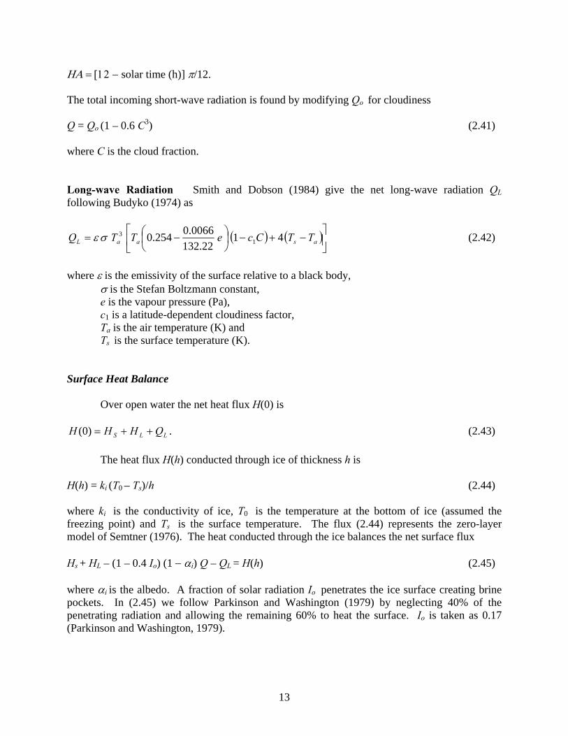
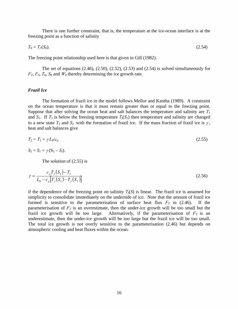
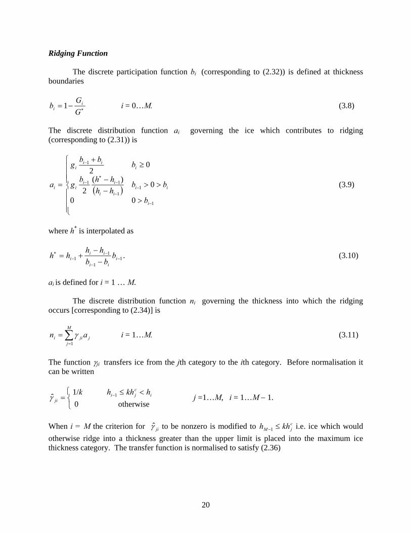
20
Ridging Function
The discrete participation function bi (corresponding to (232)) is defined at thickness boundaries
lowastminus=GG
b ii 1 i = 0hellipM (38)
The discrete distribution function ai governing the ice which contributes to ridging (corresponding to (231)) is
( )
⎪⎪⎪
⎩
⎪⎪⎪
⎨
⎧
gt
gtgtminusminus
ge+
=
minus
minusminus
minuslowast
minus
minus
1
11
11
1
00
0)(2
02
i
iiii
iii
iii
i
i
b
bbhhhhbg
bbbg
a (39)
where h is interpolated as
11
11 minus
minus
minusminus
lowast
minusminus
+= iii
iii b
bbhh
hh (310)
ai is defined for i = 1 hellip M
The discrete distribution function ni governing the thickness into which the ridging
occurs [corresponding to (234)] is
sum=
=M
jjjii an
1γ i = 1hellipM (311)
The function γji transfers ice from the jth category to the ith category Before normalisation it can be written
⎩⎨⎧ ltle
= minus
otherwise01 ˆ 1 i
cji
jihkhhk
γ j =1hellipM i = 1hellipM minus 1
When i = M the criterion for jiγ to be nonzero is modified to c
jM khh leminus1 ie ice which would otherwise ridge into a thickness greater than the upper limit is placed into the maximum ice thickness category The transfer function is normalised to satisfy (236)
21
sum=
l jlcl
cj
jiji hh
γγγ
ˆˆ i j = 1hellipM (313)
The discrete ridging function (corresponding to (230)) may now be written
( )sum =minus
+minus= M
j jj
iiri
na
naW
1
(314)
and substituted into the redistribution function (37)
34 Thermodynamic Redistribution of Ice
The implementation of the discrete thermodynamic redistribution described in this
section follows Hibler (1980) Heat budgets (243) to (245) are solved at the water surface and the surface of ice for each ice category and determine the heat flux through ice The ice growth rates fi at c
ih in the ice distribution equation (225) are determined from the heat fluxes and the ocean heat balance according to (252)
The flux of ice between categories Fi in (36) is defined from the ice growth rates by an
upstream difference
( ) )0min(0max
1
11ci
ci
iiiii hh
gfgfFminus
+=
+
++ (315)
The fluxes must satisfy two constraints The first is that the flux of ice between
categories does not change the total area of ice The second is that the change in ice volume must equal the ice grown or melted With M ice categories the rate of change in ice area per unit area expressed in terms of fluxes is
( )sum=
minus minusM
iii FF
11 (316)
The change is zero provided that F0 = FM = 0 Considering the second constraint the rate of change of volume of ice grown or melted per unit area is
sum=
M
iii gf
1 (317)
Expressed in terms of the fluxes the rate of change in ice volume is
22
( )sum=
minus minusM
i
ciii hFF
11
( )summinus
=+ minus=
1
11
M
i
ci
cii hhF
( ) ( )[ ]summinus
=+++=
1
111 )0min0max
M
iiiii gfgf (318)
( ) ( )summinus
=
++=1
20min0max
M
iMMiiii gfgfgf
(317) and (318) are equal except in the case of f1 negative (open water is absorbing heat) and the case of fM positive (ice from the thickest category is growing) The fluxes Fi in (315) must then be modified to account for these two cases in addition to the requirements following (316)
Open Water Absorbing Heat
In the case of open water absorbing heat we specify that the heat is mixed under the ice and contributes to melt at the bottom surface of the ice We modify the rates of change of ice thickness to if prime
( )⎩⎨⎧
gtminus+=
=prime1110
1 iAfAfi
fi
i (319)
where A is the total ice concentration Note that (319) preserves the net rate of ice growth
sumsum==
=primeM
iiii
M
ii gfgf
11 (320)
Growth of Thickest Ice Category
The second case in which flux of the form (315) does not balance the change in ice volume is when the thickest ice is growing In this case we add thick ice growth proportionally to all ice categories Let
hgfC MM=1 (321)
Then define the flux
23
⎩⎨⎧
gt=minus
=1
1
1
1 igC
iACF
iithick (322)
The flux (322) has the property that the increase of ice area is balanced by a decrease in
open water area Note also that the total rate of increase in ice volume from Fthicki balances the rate of increase of volume from growth of the thickest ice category ie
MMci
M
iithick gfhF =sum
=2 (323)
Maximum Rate of Decay
Hibler (1980) suggests applying a maximum rate of ice decay (minimum growth rate) fmin taken here as minus015 m day-1 We modify the ice growth rates
( ) iimini gfff prime=primeprime max (324)
The difference between ii ff primeprimeprimeand represents excess heat which melts ice laterally The excess rate of decay is
( ) i
M
iii gffExcess sum
=
primeminusprimeprime=1
(325)
Similarly to the thick ice growth we allocate this decay proportionately to all ice categories Define
hExcessC =2 (326)
then the lateral melt in terms of a flux is
⎩⎨⎧
gtminus=
=1
1
2
2 igC
iACF
iilateral (327)
The redistribution of ice from growth or melt can be finally written as
ithickilateraliii FFFF
tg
1 ++minus=Δ
Δminus (328)
24
4 Canadian East Coast Ocean Model (CECOM)
The region of interest for the model extends from the Gulf of Maine in the south to Baffin Bay in the north The model is implemented on a spherical coordinate system To reduce the impact of converging meridians we select a spherical coordinate system that is rotated relative to the earthrsquos longitude and latitude so that the equator of the rotated system bisects the domain In the following sub-sections the coordinate transformation and model domain are described
41 Rotated Spherical Coordinates
The relation between Cartesian coordinates (x y z) and longitude and colatitude (φ θ) (refer to Figure 41) is x = sinθ cosφ y = sinθ sinφ (41) z = cosθ where we take the radius of the sphere as unity Consider the transformation from original coordinates r to coordinates in a rotated system rprime
⎟⎟⎟
⎠
⎞
⎜⎜⎜
⎝
⎛=
zyx
r rArr ⎟⎟⎟
⎠
⎞
⎜⎜⎜
⎝
⎛
primeprime=prime
zyx
r (42)
A rotated system can be defined by the successive application of three rotations (Figure 42) 1 angle ξ about the z axis 2 angle η about the new y axis and 3 angle ζ about the new z axis The angle of rotation is in the clockwise direction looking in the direction of the axis The transformations from r to rprime and components of vectors are given in Appendix 2
25
Figure 41 Spherical coordinate system with longitude φ and co-latitude θ
Figure 42 The decomposition of a coordinate system rotation into three successive rotations of ξ η and ζ The red line is the y axis after one rotation 42 The CECOM Domain
The CECOM model grid has a resolution of 01deg times 01deg As noted it is defined on a rotated spherical coordinate system (Figure 43) The model domain in the geography
26
coordinates and the inner and outer boundaries are shown in Figure 44 The bathymetry of the domain is drawn in Figure 45 Specifics of the domain are given in Table 41
Generalised sigma coordinates are used to retain near-surface resolution even as bottom
depth increases The procedure we use to select the vertical levels is somewhat arbitrary For sufficiently deep water (bottom depth greater than or equal to H1) we specify that a fixed upper layer and the underlying ocean each have a given number of levels The levels are scaled according to the fixed upper or varying lower layer thickness For shallow water (bottom depth less than or equal to H0) all levels are distributed uniformly Between H0 and H1 the levels are linearly interpolated between the levels for H0 and H1
H0 = 10 m H1 = 64 m and an upper layer thickness of 64 m are selected There are a
total of 21 levels with 8 levels in the upper layer and 13 levels in the underlying ocean (at depths greater than H1) These generalised coordinates are shown for a section across the Labrador shelf (27deg longitude in rotated coordinates) in Figure 46
Figure 43 CECOM grid defined by a rotated spherical coordinate system Lines of longitude and latitude in the rotated system are drawn in red
27
Figure 44 CECOM domain (green) in the geographic coordinates The double red lines are the inner and outer boundaries of the model The blue box is the boundary in the rotated system of Fig 43
28
Table 41 Specifications of the CECOM domain ________________________________________________________________________ Coordinate rotation ( ) )1718241( degminusdegdeg=ςηξ Extent (rotated coordinates) 0 to 40deg longitude minus11 to 103deg latitude Horizontal resolution 01deg times 01deg
Dimension 400 times 213 times 21 (east times north times vertical) 410 times 223 times 21 including boundary relaxation zones time step 450 s (internal) 15 s (external) ________________________________________________________________________
Figure 45 The bathymetry of the CECOM domain Depth contours of 200 1000 2000 hellip m are drawn Specified transports (Sv) at open ocean boundary are indicated
29
Figure 46 A cross-section of the generalized coordinates across the Labrador Shelf The upper panel shows the coordinates over the upper 200 m 43 Ocean Initial State Boundary Conditions and Model Spin-up
Monthly climatological ocean temperature and salinity are used as an initial state and as open ocean boundary conditions The monthly climatologies were obtained from an objective analysis of historical data archived at Bedford Institute of Oceanography (Tang 2007) The database covers an area from northern Baffin Bay to Cape Hatteras and from the coast to 42deg W It is derived from a variety of sources dating back to 1910 The objective analysis employed an iterative difference correction procedure with topography-dependent radii of influence The grid resolution is 16deg times 16deg Figure 47 is a sample plot from the data set showing surface temperature and salinity for September
30
Figure 47 Surface temperature and salinity for September from objective analysis The red dots are the locations of the raw data
31
Transports based on large-scale models and observations are specified at the open boundaries of the model (Clarke1983 Ezer and Mellor 1994) In the present implementation the transports as shown in Figure 45 are used Different specifications are being tested to obtain best results The vertical profile of normal velocity is determined by the density through the geostrophic relation The sea level elevation at the open boundaries is determined by geostrophy to within a constant
The model open ocean boundary (double red lines in Fig 44) is interrupted by land masses The procedure to determine sea level in the ocean straits (Nares Strait Lancaster Sound Jones Sound Hudson Strait and St Lawrence Estuary) is as follows We spin up the model with three diagnostic runs of 10 days duration each with zero wind stress The sea level at open boundaries of straits is set to the adjacent interior value from the end of the previous run The spin-up concludes with a 10-day prognostic run
The initial state consists of September temperature and salinity and zero ice We create
12 open ocean boundary conditions corresponding to the monthly temperature and salinity fields As noted previously the geostrophic relation determines sea level elevation only to within a constant The constants ie the sea level average across open boundaries in straits are determined from the spin-up The monthly boundary conditions are linearly interpolated to daily values The sea level elevation and transport stream function after the spin-up process are drawn in Figure 48
Figure 48 The sea level elevation (left) and transport stream function (right) following the spin-up process
32
44 Ice categories
The ice model is implemented with 10 ice thickness categories with boundaries at 005 018 038 066 106 158 224 304 398 and 504 m The corresponding central thicknesses c
ih are 0 012 028 052 086 132 191 254 351 and 451 m 5 Model Physics of WaveWatch III (WW3)
The WAVEWATCH III (hereafter WW3) wave model (version 222) is used in the BIO forecasting system to forecast wave height and direction This is a WAM-type ocean surface wave model developed at NOAANCEP (Tolman and Chalikov1996 Tolman 2002) It has been successfully applied in global and regional scale studies in many areas including the North Atlantic and has proven to be an effective tool to study wave spectral evaluation air-sea interactions and nonlinear wave-wave interactions WW3 is a discrete spectra and phase-averaged model (Battjes 1994)
For regional and global applications the directional wave spectrum is resolved at each model grid point in terms of wavenumber-direction bands and the evolution of the wave field is found by numerically solving the spectral wave action balance equation which is usually written as
σθ
θλ
λθφ
φφSNNk
kNN
tN
g =partpart
+partpart
+partpart
+partpart
+partpart ampampampamp cos
cos1 (5-1)
where λ is longitude φ is latitude θ is wave propagation direction k is wave number t is time σ is the intrinsic angular frequency WW3 evaluates the balance equation for the wave action spectrum )( txkN θ which is usually expressed in spherical coordinates (Komen et al 1994)
The derivatives in (5-1) are the propagation velocities in physical and spectral domains
RUcg φθ
φ+
=cosamp
φθ
λ λ
cossinR
Ucg +=amp
Rcg
g
θφθθ
costanminus= ampamp R is the radius of the earth and
φU and λU are current components in φ and λ directions The left side of equation (1) represents the local rate of change of wave action density propagation in physical space action density shifting in frequency and direction due to the spatial and temporal variation in depth and current The net source term S consists of wind input( inS )white-capping dissipation( dsS ) nonlinear wave-wave interactions( nlS ) and bottom friction( botS ) WW3 uses an explicit scheme to solve the action balance equation (1) for N
Two combinations of the source terms inS and dsS are available in WW3 The default set up of WW3 corresponds to the wave-boundary layer formulation for inS and dsS due to Tolman and Chalikov (1996) Tolman (2002) notes that application of this formulation has entailed a
33
correction in fetch-limited wave heights that results from atmospheric stratification which necessitates a re-tuning of the model by defining an lsquoeffectiversquo wind as well as an additional correction for the impact of stability on wave growth An alternate combination corresponds to WAM cycle 3 physics (hereafter denoted WAMC3 physics) in which inS and dsS are based on WAMDI (1988) Snyder et al (1981) and Komen et al (1994) Quadruplet nonlinear interactions nlS are simulated by DIA and bottom dissipation bfS by the JONSWAP parameterization of Hasselmann et al (1973) Padilla-Hernatildendez et al [2007] compared the WW3 model against WAM and SWAN models for two North Atlantic storms and found that WW3 provided the high quality statistical comparisons to deep water observations 6 The Bedford Institute Ocean Forecasting System (BIOFS) BIOFS is a real-time short-term (2-day) forecasting system for eastern Canadian waters The forecast period is constrained by input data from Environment Canada If meteorological data from long range weather forecasts are available the ocean forecasts can be extended to a longer period It consists of two sub-systems one for CECOM (Section 63) and one for WW3 (Section 64) Graphic display of the forecasts can be viewed at the following public website maintained by DFO httpwwwmardfo-mpogccascienceoceanicemodelice_ocean_forecasthtml The parameters displayed on the website are surface trajectories water level time series at selected locations ice concentration and thickness wave height and direction (Northwest Atlantic and Atlantic Maritimes) sea surface elevation (non-tidal) maps temperature at surface and 50 m They are given at hourly (water level time series) 6-hourly (wave) or 12-hourly (all others) intervals 61 Input Data Meteorological Data Meteorological forcing is taken from the Canadian Meteorological Centre (CMC) Global Environmental Multiscale (GEM) model (Mailhot et al 2006) which provides 48 hour forecasts twice daily at 0000 and 1200 UTC with fields output at 3 hour intervals The GEM model is an operational atmospheric model that is part of the Canadian Regional Forecast System (RFS) developed by Environment Canada The model uses a variable resolution grid over the entire globe with a mesoscale 15 km horizontal resolution window over Northern America Fields used in the forecasting system are 10m winds 2m air and dew point temperatures total cloud coverage and total accumulated precipitation All meteorological parameters are linearly interpolated to the ocean and wave model grids Except for the10 m winds the parameter values change every 3 hours For CECOM the 10m wind field is interpolated in time to the model time step of 75 minutes to avoid temporal discontinuities in the dynamical forcing Total accumulated
34
precipitation is converted to a precipitation rate For WW3 the wind fields are interpolated to the propagation time step of the respective wave model (see Section 64 for details) Sea-Ice Data Ice concentration data are used for data assimilation (Section 62) in the ice model and to define the wave domain in WW3 In WW3 a grid point is considered open ocean if the ice concentration is equal or less than 05 Otherwise it is considered land Digital sea ice charts which include ice concentration data are provided by Canadian Ice Services(CIS) Canadian waters are covered by five digital ice charts (Figure 61) Data from Eastern Arctic Hudson Bay and East Coast are used in the forecasting system CIS produces daily charts for the Gulf of StLawrence and the Labrador and Newfoundland coasts south of 58N Regional charts for Hudson Bay Baffin Bay and the Labrador coast north of 58N are produced fortnightly Typically the regional charts are released several days after the date for which they are valid Since these charts represent more of a two week average condition than an instantaneous one BIOFS uses a regional charts release date as its valid date
Figure 61 Coverage of CISrsquos digital ice charts (courtesy of CIS) The digital charts use the ldquoegg coderdquo (Environment Canada 2005) to indicate the sea ice partial concentration for each stage of development on a regularly spaced grid Each ldquoeggrdquo indicates up to three different ice types (ignoring trace amounts) each of which is assigned a stage and concentration The stage of development may be interpreted as an approximate
35
measure of the ice thickness The conversion of stage to ice model thickness category is illustrated in Table 61 There are also four special cases listed in Table 62 Table 61 Conversion from ice stage to ice model category
Ice stage of development Description
Ice model
categoryIce thickness
boundaries (m)
OW BW IF Open Water bergy water ice-free 1 -005 lt h le 005
1 New 2 005 lt h le 018
2 Nilas 2 005 lt h le 018
3 Young Unknown 3 018 lt h le 038
4 Young Grey 2 005 lt h le 018
5 Young Grey-White 3 018 lt h le 038
6 First Year Unknown 4 038 lt h le 066
7 First Year Thin 5 066 lt h le 106
8 First Year Thin First Stage 5 066 lt h le 106
9 First Year Thin Second Stage 5 066 lt h le 106
1 First Year Medium 6 106 lt h le 158
4 First Year Thick 7 158 lt h le 224
7 Old 8 224 lt h le 304
8 Old Second Year 9 304 lt h le 398
9 Old Multi-Year 9 304 lt h le 398
L Ice of Land Origin 9 304 lt h le 398
B Brash 3 018 lt h le 038
Each stage of development is first converted to a category The partial concentrations
and categories including flags (Table 62) are then nearest-neighbour interpolated to the model grid Grid points with land fast ice will be filled with neighbouring concentrations and categories Including flags in the interpolation preserves grid points which should not be filled by interpolation All the charts available for a forecast date are then combined Where charts overlap the concentrations of each category are averaged Flagged points are ignored in the averaging
36
Table 62 Interpolation of ice data
Ice stage of
development Description Action
POINT NOT COVERED BY
POLYGON Point is outside CIS analysis area Flag
LAND Land point Flag
ICEGLACE Useless CIS category indicating ice presence but not providing concentration or stage
Flag
FASTICE Land fast ice Nearest Neighbour
Tides Tidal constituents of elevation and velocity come from two sources Paturi et al (2008) provides eight constituents (M2 S2 N2 K2 K1 O1 P1 Q1) and covers most of the model domain up to Davis Strait Dunphy et al (2005) provides five tidal constituents (M2 S2 N2 K1 O1) for Baffin Bay Constituents are linearly interpolated to the model grid Where the two sources slightly overlap at Davis Strait matching constituents are averaged 62 Data assimilation in CECOM
Many assimilation schemes have been developed for oceanographic and meteorological applications in the past 20 years Advanced schemes such as 3-d and 4-d variational method and Karmen filter require massive resources and abundant data to yield optimum results In this section we describe three methods to assimilate the annual cycle of the temperature and salinity fields sea surface temperature and ice concentration data into the ocean forecast model Assimilation of the Annual Cycle of the Temperature and Salinity Fields Monthly temperature and salinity climatologies are prescribed at the open boundaries of CECOM Such constraints are not strong enough to prevent the temperature and salinity fields from drifting in multi-year integration To ensure the annual cycles are preserved a nudging term with a constant relaxation time scale tR of 45 days are added to the temperature and salinity equation
37
)(1 TTtt
TCLIM
R
minus+=partpart
)(1 SStt
SCLIM
R
minus+=partpart
where TCLIM and SCLIM are monthly temperature and salinity climatologies linearly interpolated to daily intervals Assimilation of Sea Surface Temperature Data Daily near real-time sea surface temperature (SST) derived mainly from satellite observations are provided by CMC The data are assimilated into the ocean forecast model using a flux correction method The method is based on the theory of optimal interpolation A correction term proportional to the differences between the modeled and observed SST is added to the heat flux equation
We first consider the equation for SST assimilation (see Appendix 4)
( ) [ ])()(
2exp)()( 2
2
22
2
om
ooo
om
mma tTtTtt
tTtT minus⎥⎥⎦
⎤
⎢⎢⎣
⎡ minusminus
++=
τεεε
(61)
where the superscripts and subscripts ldquoardquo ldquomrdquo and ldquoordquo in (61) denote ldquoassimilationrdquo ldquomodelrdquo and ldquoobservationrdquo respectively to is the time of the most recent observation and t is the model time 2
mε and 2oε are the model and data errors respectively τ is the correlation time scale of
SST Since change in SST ΔT is related to change in heat flux ΔQ by
Qhc
tT
p
d Δ=Δρ
where h is the mixed layer depth and td is the time interval of SST data the first terms on each side of (61) can be replaced by the corresponding heat fluxes The equation for SST data assimilation is
( ) [ ])()(2
exp)()( 2
2
om
ooo
d
pma tTtTtt
Ft
hctQtQ minus
⎥⎥⎦
⎤
⎢⎢⎣
⎡ minusminus+=
τρ
(62)
where F = 1 [1+ (εο εm)2] F ranges from 0 to 1 Not all parameters in (62) are well known To implement (62) in the forecast model the parameters are adjusted to yield optimal results
38
Figures 62 and 63 show the impact of data assimilation on model SST from a test run In this run F = 1 td = 1 day τ = 1 day were used and h = 20 m To reduce model noise in the run )( o
m tT in (62) was replaced by the model SST averaged over the previous day (from t0 - 1 day to t0) Significant improvements in the model SST can be achieved by using this assimilation scheme Without data assimilation the difference between the model and data at the Scotian Shelf is of the order of ~ 2o C The difference is reduced to a fraction of a degree with data assimilation Over the model domain the model without data assimilation over predicts SST in the northern Labrador Sea and under predicts SST in the coastal and the North Atlantic Current regions (Figs 63) Data assimilation is able to reduce the errors to less than 1o C
The SST assimilation is applied to ice free waters only In ice covered areas the sea
surface temperature is equal or very close to the freezing temperature
Figure 62 A comparison of SST in a 1o x 1o area centered at the indicated location with and without data assimilation
39
Figure 63 CMC SST (left) and the difference between the model and data with (middle) and without (right) data assimilation Assimilation of sea-ice data An insertion-nudging method is used for ice data assimilation Ice concentration data are inserted to the model gradually and the model concentration is restored to the data value with a prescribed time constant In the equation for the thickness distribution function a term proportional to the difference between the observed and values is introduced
( ) ( ))( ioi
iiice
i ggdiffusionhfg
gt
gminusΓ++Ψ=
partpart
+sdotnabla+part
partu (62)
where goi is the ice chart concentrations and gi is the model concentrations for ice of thickness category i Γ has the following form
⎥⎦
⎤⎢⎣
⎡ minusminus=Γ 2
2
2)(
expw
om
ttγ
γ (63)
where t is the model time to is the time for which the ice chart is valid γm and γw are adjustable parameters The Gaussian function in (63) limits nudging to the times around the ice chart time 1γm is the restoring time scale In the present implementation the values of 1γm and γw are set to 16 hours (5760 seconds) and 3 hours (10800 seconds) respectively At one hour from the ice chart time this scheme gives a concentration change rate of ~05 per hour At times plusmn 2γw from
40
the ice chart time the rate is negligible Where there is no ice chart data the nudging is not applied Figure 64 is a comparison of ice area south of 58o with and without data assimilation for January 2008 Figure 65 shows the ice concentration from CISrsquos East Coast ice chart and the model results with and without data assimilation The data assimilation significantly reduces the model error In particular ice cover in the Gulf of St Lawrence and the location of the eastern ice edge can be simulated more realistically with data assimilation
Figure 64 A comparison of the model ice area south of 58o N with (blue) and without (black) data assimilation The unit is percentage of the model area south of 58o N
41
Figure 65 Ice concentration for January 28 2008 data (left) model results without (middle) and with (right) data assimilation 63 Operational Implementation of CECOM The ice-ocean component of BIOFS is mostly comprised of MATLAB scripts that handle the pre-processing of model input fields the execution of the CECOM FORTRAN executable the post-processing of model results and the management of data files MATLAB was chosen for its platform independence interpolation and graphics functionalities and the abundance of open source tools such as M_Map (Pawlowicz 2006) readgrib (Blanton 2005) snctools (Evans 2007) and T_Tide (Pawlowicz et al 2002) Scheduling and automation is handled by the Linux bash shell but could easily be implemented for other platforms and operating systems Delivery of Meteorological and ice Data
As with any endeavor in real-time forecasting the primary concern is the timely delivery of the data required to force the forecast model To address this concern a separate subsystem written in bash shell scripts automates the retrieval of crucial meteorological forecast data transmitted from CMC to BIO server Emerald2 twice a day The subsystem polls the site for data and performs file checks after retrieval to verify file integrity There is usually a 5-6 hour delay between the CMC regional forecast and the appearance of the forecast data on their ftp site If the system fails to retrieve the data it retries for a predefined number of times The digital ice charts valid for 1800 UTC are delivered daily to an ftp server at BIO Starfish at ~2200 UTC The CIS delivery system itself checks for file integrity after delivery
42
Forecast Schedule CECOM is run three times daily within BIOFS producing 48 hour forecasts for 0000 and 1200 UTC (Table 63 Fig 66) Due to delays in receiving the meteorological data the CMC 1200 UTC data are received at ~1700-1800 UTC and the forecast completes at ~1800-1900 UTC A 1200 UTC data assimilation run using 1800 UTC sea ice concentration data and 1200 UTC sea surface temperature data (the same SST are received in the CMC 0000 UTC forecast data) is made the following morning at ~0300 UTC to assimilate the most recent ice chart and sea surface temperature data The 0000 UTC forecast is run four hours following the data assimilation run at ~0700 UTC Table 63 Ocean forecast schedule Both the local time ldquoATrdquo (Atlantic Time) and UTC are indicated
Day 1 Day 2
1 ndash 2 pm AT 2 ndash 3 pm AT 6 pm AT 11 pm AT 1 ndash 2 am AT 3 am AT
1700-1800 UTC 1800-1900 UTC 2200 UTC 0300 UTC 0500-0600 UTC 0700 UTC
CMC 1200 UTC forecast data
received
1200 UTC 48-hour forecast
CIS charts received
1200 UTC 48-hour ice
and SST assimilation
CMC 0000 UTC forecast data received
0000 UTC 48-hour forecast
43
Figure 66 Flow chart of the forecasting operations in a 24-hour period Forecast Methodology Each forecast is initialized with the most recent output of a previous forecast The ocean lateral boundary conditions are linearly interpolated to daily values from the monthly means to prevent discontinuity The boundary conditions also provide a constraint for temperature and salinity near the boundaries In the interior nudging and statistical interpolation are used to prevent long-term drifts and to assimilate sea surface temperature data into the model (see Section 62)
CMC 1200UTC data
CIS 1800UTC data
CMC 0000UTC data
12 UTC
forecast run
Data assim
ilation run
00 UTC
forecast run
1200 UTC forecasts
0000 UTC forecasts
Day 1 Day 2 Day 3
Ice concentration data
Sea surface temperature data
Add tide and Stokes drift
Add tide and Stokes drift
44
After the model run T_Tide (RPawlowicz et al 2002) calculates the tidal current and
elevation for the forecast period The tidal components are then linearly added to the forecast components For surface currents wave induced Stokes drifts are added to the model surface current to obtain the total surface current (Tang et al 2007) The Stokes drift us is obtained from the 2-dimensional wave spectrum E (f θ) of WW3 by integrations over frequency and direction
( )intint= θθπ dfdfEef kz
s 4 2ku (64)
where f is wave frequency θ is wave direction k is wave number and k is the magnitude of k
There are two options for the Strokes drift in the forecasting system us can be computed directly from (64) at every model grid point A simpler method is to parameterize us by surface winds us = a W + b W2 (65)
β = turning angle (positive for clockwise) relative to wind direction (66) where us and β are the magnitude and direction of us respectively and W is 10 m wind speed The parameters a b and β are determined from least-squared fits of the Strokes velocities computed from (64) for October-December 2007 In most applications (eg surface drifter floating object) vertically averaged surface currents are required The Stokes velocities in (65) and (66) are replaced vertically averaged Stokes velocities The results of the least-squared fits are given in Table 64 for different depths of averaging Table 64 Parameters values of the Stokes drift for different depths of averaging Depth (m) 1000a 1000b β (deg)
1 2525 0641 380 2 1656 0533 400 3 1176 0459 410 4 0889 0405 430 5 0699 0363 440
Drift tracks are calculated from the total surface current field Each track starts at a model grid point and is advected by the surface current Horizontal linear interpolation is used to calculate the surface current field between grid points Distances are calculated using the plane sailing method which ignores the earths curvature
45
For ice forecasts all available 1800 UTC ice charts from the previous day are processed and assimilated into the model to correct the model ice field as described in Section 62 For ocean forecasts 1200 UTC SST data from the previous day are assimilated into the model (Figure 66) 64 Operational Implementation of WW3
The wave models are implemented on a system of three nested grids (Figures 67 68 69 and Table 65) The spatial resolution increases from 10o in the coarse grid to 05o in the intermediate grid to 01667o (10rsquo) in the fine resolution grid This system of grids ensures that energy from distant storms is not lost in simulating storms making landfall in coastal areas of North America The grid dimensions and resolutions are given in Table 65 Etopo2 bathymetry is used from the United States National Geophysical Data Center at 2 minutes resolution WW3 is used for the coarse intermediate and fine resolution simulations Following the Courant-Friedrichs-Leacutevy (CFL) stability criterion the propagation time steps for WW3 are 20 and 10 minutes for the coarse and intermediate grids respectively and 4 minute propagation steps for the fine-resolution grid In Table 65 WW3 has 4 time steps Δtg is the global time step by which the entire wave model solution is propagated forward in time Δtρ1 is the maximum spatial (xy) propagation time step for the lowest frequency which is required to satisfy the CFL criterion Δtis is the maximum intra-spectral (k θ) propagation time step which is also required to satisfy the CFL criterion and Δtst is the minimum time step for the integration of the source terms which is dynamically adjusted for each grid and for Δtg
WW3 interpolates the wind fields to the propagation time step of the respective wave model For fast moving storms WW3 has a built-in scheme to reduce the source term integration time step when the situation is changing rapidly Moreover in WW3 the source term integration time step can be set by the user Thus we set the minimum source term time step to 5 minutes in the coarse-resolution grid to adequately simulate the storms considered here For the intermediate and fine grids source term time steps were both set to 25 (see Table 65) Details regarding the spectral range and resolution of the WW3 model are given in Table 66 in terms of the lowest and highest frequencies ( lowf and highf ) number of points ( n ) frequency resolution ( fΔ ) and angular resolutions ( θΔ ) The 48-hour WW3 wave forecasts run twice daily (0000 UTC and 1200UTC) WW3 simulates waves outside nearshore areas where shallow water wave processes are not important The model includes standard physics for wave propagation growth by wind nonlinear interactions dissipation due to whitecapping and dissipation due to bottom friction In coastal estuary and nearshore areas where water depth is shallow fine-resolution computational domains are sometimes needed for dedicated studies nested within coarserndashresolution basin-scale domains in order to resolve complex topography coastline features and shallow water wave physics In these special cases an option is that the shallow water SWAN wave model (version 4031) can be applied for a fourth domain nested within the third domain (Ris et al 1994 Booij et al 1996 Booij et al 1999 Holthuijsen et al 2003 Booij 2004) in these specific areas The physics of SWAN are different from that of WW3 especially for shallow water waves
46
SWAN can simulate shoaling refraction bottom friction and depth-induced wave breaking besides the processes for whitecapping wind input and nonlinear wave-wave interactions that are present in WW3 SWAN is formulated in terms of an action balance equation Xu et al (2007) describe the implementation of WW3 and nested grids for the North Atlantic and SWAN for Lunenburg Bay for studies related to the waves generated by hurricane Juan (September 28-29 2003)
Figure 67 Model domain of WW3 - Atlantic Ocean and sample model output (0600 UTC November 4 2007) The colors indicate significant wave height The arrows indicate wave period and direction
47
Figure 68 Model domain of WW3 ndash Northwestern North Atlantic Ocean and sample model output (0600 UTC November 4 2007) The colors indicate significant wave height The arrows indicate wave period and direction
48
Figure 69 Model domain of WW3 ndash Atlantic maritimes and sample model output (0600 UTC November 4 2007) The colors indicate significant wave height The arrows indicate wave period and direction
49
Table 65 Geographical location of the grids used in this study λ θΔ are the resolutions in longitude λ and latitudeφ and Nλ and Nφ are the number of points in λ and φ Finally tΔ is the propagation time step and tΔ ST is the required time step for source term integration for the three models as required to satisfy the CFL criterion GRIDS Longitude Latitude λ θΔ Nλ Nφ Δtg tΔ ST
Coarse 40oE ndash 82oW 75oSndash 77oN 1o 123 153 20 min 50 min
Intermediate 40oWndash75oW 20oN-75oN 05o 71 111 10 min 2min
Fine 47oWndash71oW 42oN-52oN 10rsquo 145 61 5 min 25 min
Table 66 Spectral domains for all models lowf highf are the default values
Parameters Value
lowf highf [s-1] 00418 06028
nf fΔ 29 11 ftimes
θn θΔ 36 10o
50
References Battjes JA 1994 Shallow water wave modelling Proc Int Symp Waves -Phys Numerical
Modelling University of British Columbia Vancouver I 1-23 Budyko MI 1974 Climate and Life Academic Press New York 508 pp Blanton B 2005 readgrib
httpwwwopnmlunceduOPNML_Matlabread_gribread_gribhtml Blumberg AF and GL Mellor 1987 A description of a three-dimensional coastal ocean
circulation model in Three-Dimensional Coastal Ocean Models Coastal Estuarine Sci 4 edited by NS Heaps pp 1-16 AGU Washington DC
Booij N LH Holthuijsen and RC Ris 1996 The ldquoSWANrdquo Wave Model For Shallow Water
Coastal Engineering 1 668~672
Booij N RC Ris and LH Holthuijsen 1999 A third-generation wave model for coastal regions Part I Model description and validation J Geophys Res 104 C4 7649-7666
Booij N 2004 SWAN Cycle III version 4041 user manual[Available online at httpfluidmechanicstudelftnlswanindexhtm]
Carton JA G Chepurin and X Cao 2000 A simple ocean data assimilation analysis of the
global upper ocean 1950-95 Part I methodology J Phys Oceanogr 30 294-309 Charnock H 1955 Wind stress on a water surface Quarterly Journal of Royal Meteorological
Society 81 pp 639ndash640 Clarke RA 1984 Transport through the Cape Farewell-Flemish Cap section Rapp PV Reun
Cons Int Explor Mer 185 120-130 Dunphy M F Dupont C G Hannah D Greenberg 2005 Validation of a modelling system for
tides in the Canadian Arctic Archipelago Can Tech Rep Hydrogr Ocean Sci 243 vi + 70 pp
Dunlap E BM Detracey and CL Tang 2007 Short-wave radiation and sea ice in Baffin Bay
Atmosphere-Ocean 45 195-210 Environment Canada 2005 ldquoMANICE - Manual of Standard Procedures for Observing and
Reporting Ice Conditionsrdquo httpice-glacesecgcca AppWsvPageDspcfmLang=engamplnid=23ampScndLvl=noampID=172
Evans J 2007 snctools httpmexcdfsourceforgenet
51
Ezer T and GL Mellor 1994 Diagnostic and prognostic calculations of the North Atlantic circulation and sea level using a sigma coordinate ocean model J Geophys Res 99 14159-14171
Flato GM 1994 McPIC Documentation for the multi-category particle-in-cell sea ice model
Can Tech Rep Hydrogr Ocean Sci 158 74 pp Gill AE 1982 Atmosphere-Ocean Dynamics Academic Press New York 662 pp Hasselmann K TP Barnett E Bouws H Carlson DE Cartwright K Enke JI Ewing H
Gienapp DE Hasselmann P Kruseman A Meerbrug P Muumlller DJ Olbers K Richter W Sell and H Walden 1973 Measurements of wind-wave growth and swell decay during the Joint North Sea Wave Project (JONSWAP) Dtsch Hydrogr Z A8(12) 95 pp
Hibler WD 1979 A dynamic thermodynamic sea ice model J Phys Oceanogr 9 815-846 Hibler WD 1980 Modeling a variable thickness sea ice cover Mon Wea Rev 108 1943-
1973 Holthuijsen L H and HN Booij 2003 Phase-decoupled refraction-diffraction for spectral
wave models Coastal Engineering 49 291-305 Jerlov NG 1968 Optical Oceanography 194 pp Elsevier Komen G J LCavaleri M Donelan M Hasselmann S Hasselmann P A E M Janssen
1994 Dynamics and Modeling of Ocean Waves Cambridge University Press 520pp Mailhot J S Beacutelair L Lefaivre B Bilodeau M Desgagneacute C Girard A Glazer A-M Leduc
A Meacutethot A Patoine A Plante A Rahill T Robinson D Talbot A Tremblay P Vaillancourt A Zadra A Qaddouri 2006 The 15-km Version of the Canadian Regional Forecast System Atmos-Ocean 44 133-149 DOI 103137ao440202
Martinsen EA and H Engedahl 1987 Implementation and testing of a lateral boundary
scheme as an open boundary condition in a barotropic ocean model Coastal Eng 11 603-627
Mellor GL and AF Blumberg 1985 Modeling vertical and horizontal diffusivities with the
sigma coordinate system Mon Wea Rev 113 1380-1383 Mellor GL and LH Kantha 1989 An ice-ocean coupled model J Geophys Res 94
10937-10954 Mellor GL and T Ezer 1991 A Gulf Stream model and an altimetry assimilation scheme J
Geophys Res 96 8779-8795
52
Mellor GL S Hakkinen T Ezer and R Patchen 2002 A generalization of a sigma coordinate ocean model and an intercomparison of model vertical grids in Ocean Forecasting Conceptual Basis and Applications edited by N Pinardi and J Woods pp 55-72 Springer Berlin
Mellor GL and AF Blumberg 2004 Wave breaking and ocean surface layer thermal
response J Phys Oceanogr 34 693-698 Padilla-Hernatildendez R W Perrie B Toulany and P C Smith 2007 Intercomparison of third
generation wave models Weather and Forecasting Vol 22 No 6pages 1229-1242 Parkinson C L and W M Washington 1979 A large-scale numerical model of sea ice J
Geophys Res 84 311-337 Paturi S G Han and B deYoung 2008 A 3-D multi-constituent data assimilative tidal model
of the northwest Atlantic Atmosphere-Ocean Submitted Paulson CL and JJ Simpson 1977 Irradiance measurements in the upper ocean J Phys
Oceangr 7 952-956 Pawlowicz R 2006 M_Map httpwwweosubcca~rich Pawlowicz R B Beardsley and S Lentz 2002 Classical tidal harmonic analysis including
error estimates in MATLAB using T_TIDE Computers and Geosciences 28 929-937 httpwwweosubcca~rich
Perrie W Gunther H Rosenthal W and Toulany B 1989 Modelling wind - generated
surface gravity waves using similarity Quart J Roy Met Soc 115 1373-1396 Ris RC Holthuijsen LH and Booij N 1994 A Spectral Model for Waves in the Near shore
Zone Coastal Engineering 1 68~78 Semtner AJ 1976 A model for the thermodynamic growth of sea ice in numerical
investigations of climate J Phys Oceanogr 67 379-389 Shine KP 1984 Parameterization of the shortwave flux over high albedo surfaces as a
function of cloud thickness and surface albedo Q J R Meterol Soc 110 747-764 Sloslashrdal LH EA Martinsen and AF Blumberg 1994 Modeling the response of an idealized
coastal ocean to a traveling storm and to flow over bottom topography J Phys Oceanogr 24 1698-1705
Smith SD 1988 Coefficients for sea surface wind stress heat flux and wind profiles as a
function wind speed and temperature J Geophys Res 93 15467-15472
53
Smith SD and FW Dobson 1984 The heat budget at Ocean Weather Station Bravo Atmos-Ocean 22 1-22
Snyder RL FW Dobson JA Elliot and RB Long 1981 Array measurements of
atmospheric pressure fluctuations above surface gravity waves J Fluid Mech 20 1166-1174
Tang CL 2007 High-resolution monthly temperature and salinity climatologies for the
northwestern North Atlantic Ocean Canadian Data Report of Hydrography and Ocean Sciences No 169 iv + 55 pp
Tang CL Q Gui and I Peterson 1996a Modeling the mean circulation of the Labrador Sea
and the adjacent shelves J Phys Oceangr 26 1989-2010 Tang CL and Q Gui 1996b A dynamical model for wind-driving ice modtion ndash applicaton to
ice drift on the Labrador Shelf J Geophys Res 101 28343-28364 Tang CL CK Ross T Yao B Petrie BM Detracey and E Dunlap 2004 The circulation
water masses and sea ice of Baffin Bay Progress of Oceanography 63 183-228 Tang CL W Perrie AD Jenkins BM Detracey Y Hu B Toulany and PC Smith 2007
Observation and modeling of surface currents on the Grand Banks a study of the wave effects on surface currents J Geophys Res 112 C10025 doi1010292006JC004028
Thorndike AS DA Rothrock GA Maykut and R Colony 1975 The thickness distribution
of sea ice J Geophys Res 80 4501-4513 Tolman H L 2002 User manual and system documentation of WAVEWATCH-III version
222 Technical Note [Available online at httppolarncepnoaagovwaves] Tolman H L and Chalikov DV 1996 Source terms in a third-generation wind-wave model J
Phys Oceanogr 26 2497-2518 WAMDI group 1988 The WAM model ndash a third generation ocean wave prediction model J
Phys Oceanogr 18 1775-1810 Xu F W Perrie B Toulany and P C Smith 2007 Wind-generated waves in Hurricane Juan
Ocean Modelling Vol 16 pages 188ndash205 Yao T CL Tang and IK Peterson 2000 Modeling the seasonal variation of sea ice in the
Labrador Sea with a coupled multi-category ice model and the Princeton Ocean Model J Geophys Res 105 1153-1165
Yao T CL Tang 2003 The formation and maintenance of the North Water Atmosphere-
Ocean 41 187-201
54
Zhang J and WD Hibler 1997 On an efficient numerical method for modeling sea ice dynamics J Geophys Res 102 8691-8702
55
Appendix 1 Turbulence closure
This appendix outlines the calculations of the vertical mixing coefficients from turbulence closure Governing equations for turbulence kinetic energy q22 and turbulence macroscale l are
)(222 2
1
322
22222
qAlB
qz
Kgzv
zuK
zqK
zzqw
yqv
xqu
tq
HHo
M
q
nablasdotnabla+minuspartpart
+⎥⎥⎦
⎤
⎢⎢⎣
⎡⎟⎠⎞
⎜⎝⎛
partpart
+⎟⎠⎞
⎜⎝⎛
partpart
+
⎟⎟⎠
⎞⎜⎜⎝
⎛part
partpartpart
=part
part+
partpart
+part
part+
partpart
ρρ
)(~ 2
1
31
22
1
22222
lqAwBq
zKglE
zv
zuKlE
zlqK
zzlqw
ylqv
xlqu
tlq
HHo
M
q
nablasdotnabla+minuspartpart
+⎥⎥⎦
⎤
⎢⎢⎣
⎡⎟⎠⎞
⎜⎝⎛
partpart
+⎟⎠⎞
⎜⎝⎛
partpart
+
⎟⎟⎠
⎞⎜⎜⎝
⎛part
partpartpart
=part
part+
partpart
+part
part+
partpart
ρρ
where
2
21~ ⎟⎠⎞
⎜⎝⎛+=
LlEw
κ
( ) ( ) 111 minusminusminus ++minus= zHzL η
κ is the von Karman constant and B1 E1 and E2 are empirical constants
The effects of wave breaking are taken into consideration through the surface boundary condition for q2 At the surface the vertical gradient of q2 is proportional to the cube of the water friction velocity (Mellor and Blumberg 2004) A consequence of this boundary condition is that the eddy viscosity is non-zero at the surface (Tang et al 2007) The boundary conditions at the surface are
⎪⎩
⎪⎨⎧
=
=part
partlowast
covered ice
free ice22
321
2
32
uBq
uz
qBCα
02 =lq
where αBC is a prescribed constant and u is the friction velocity
56
020
20
2 )( ρττ yxu +=
The boundary conditions at the ocean bottom are
02
2
321
2
=
=
lq
uBq
where u is derived from the bottom stress
The mixing coefficients KM KH and Kq can be expressed in terms of stability functions SM SH and Sq
)()( qHMqHM SSSlqKKK = The stability functions are derived from the solution of analytic equations (Blumberg and Mellor 1987) involving the vertical shear and vertical density gradient In the presence of ice the mixing coefficient is the average of the values for open ocean and for ice-covered ocean (no wave effects) weighted by ice concentration Appendix 2 Generalised sigma coordinates
Generalised sigma coordinates are derived by transforming coordinates (x y z t) to (x y s t) The vertical coordinate s is defined
)()( tyxtkyxsz η+= (A21) where s is a function of the vertical variable k which ranges from 1 at the surface to kb at the ocean bottom For the purposes of this discussion k is continuous but it is discrete for the computer implementation Since 0 =partpart xz then
0
xk
ks
xs
x partpart
partpart
+partpart
+partpart
=η
or
k
xx
ss
xk
η+
minus=partpart
Also the z derivative of (A21) gives
kszk 1
=partpart
57
For a function )( tzyxφ partial derivatives in the old coordinate system are related to partial derivatives in the new coordinate system as
1
k
tt
k
k
yy
k
xx
ss
ktt
skz
ss
kyy
ss
kxx
ηφφφ
φφ
ηφφφ
ηφφφ
+partpart
minuspartpart
=partpart
partpart
=partpart
+partpart
minuspartpart
=partpart
+partpart
minuspartpart
=partpart
We define a new vertical velocity ω as
( ) ( ) yyxxtt svsusw ηηηω ++++++=
The continuity equation in transformed coordinates (henceforth dropping the asterisks) is
0)()(
=partpart
+part
part+
partpart
+part
partky
vsx
ust
s kkk ω (A22)
The momentum equations in transformed coordinates are
( ) ( ) ( ) ( ) ( )
int int +⎟⎟⎠
⎞⎜⎜⎝
⎛partpart
partpart
+partpart
minuspartpart
+
+minus=minuspart
part+
partpart
+part
part+
partpart
xk
Mk
o
kx
o
k
xxkkkkk
Mku
sK
kdk
xsgsdk
ksgs
sgsfvsku
yuvs
xsu
tus
ρρ
ρρ
ηω 22
(A23)
( ) ( ) ( ) ( ) ( )
int int +⎟⎟⎠
⎞⎜⎜⎝
⎛partpart
partpart
+partpart
minuspartpart
+
+minus=+part
part+
partpart
+part
part+
partpart
yk
Mk
o
ky
o
k
yykkkkk
Mkv
sK
kdk
ysgsdk
ksgs
sgsfuskv
ysv
xuvs
tvs
ρρ
ρρ
ηω 22
(A24)
The heat and salt equations in transformed coordinates are
( ) ( ) ( ) ( )
Tk
Hkkk MkT
sK
kkT
yvTs
xuTs
tTs
+⎟⎟⎠
⎞⎜⎜⎝
⎛partpart
partpart
=part
part+
partpart
+part
part+
partpart ω
58
( ) ( ) ( ) ( )S
k
Hkkk MkS
sK
kkS
yvSs
xuSs
tSs
+⎟⎟⎠
⎞⎜⎜⎝
⎛partpart
partpart
=part
part+
partpart
+part
part+
partpart ω
The horizontal mixing terms become
⎥⎦
⎤⎢⎣
⎡⎟⎟⎠
⎞⎜⎜⎝
⎛partpart
+partpart
partpart
+⎟⎠⎞
⎜⎝⎛
partpart
partpart
=xv
yuAs
yxuAs
xM MkMkx 2
⎥⎦
⎤⎢⎣
⎡⎟⎟⎠
⎞⎜⎜⎝
⎛partpart
+partpart
partpart
+⎟⎟⎠
⎞⎜⎜⎝
⎛partpart
partpart
=xv
yuAs
xyvAs
yM MkMky 2
⎟⎟⎠
⎞⎜⎜⎝
⎛partpart
partpart
+⎟⎠⎞
⎜⎝⎛
partpart
partpart
=yTAs
yxTAs
xM HkMkT
⎟⎟⎠
⎞⎜⎜⎝
⎛partpart
partpart
+⎟⎠⎞
⎜⎝⎛
partpart
partpart
=ySAs
yxSAs
xM HkMkS
These forms are not simply the transformations of (28) This relates to separating vertical mixing from horizontal mixing in a coordinate system in which constant k surfaces are sloping (Mellor and Blumberg 1985 and Mellor et al 2002) Appendix 3 Rotated spherical coordinate system
Coordinates r on a unit sphere are transformed to rprime in a rotated system (42) with the matrix R by
rRRRRrr ξης==prime (A31) where Rξ Rη Rζ are transformation matrices for rotations by the individual angles ξ η and ζ respectively (Figure 42)
The individual rotation matrices are
⎟⎟⎟
⎠
⎞
⎜⎜⎜
⎝
⎛minus=
1000cossin0sincos
ξξξξ
ξR ⎟⎟⎟
⎠
⎞
⎜⎜⎜
⎝
⎛ minus=
ηη
ηη
η
cos0sin010
sin0cosR
⎟⎟⎟
⎠
⎞
⎜⎜⎜
⎝
⎛minus=
1000cossin0sincos
ςςςς
ςR (A32)
giving the matrix R as
59
⎟⎟⎟
⎠
⎞
⎜⎜⎜
⎝
⎛+minusminusminus
minus+minus
ηξηξηηςξςξηςξςξηςηςξςξηςξςξης
cossinsincossinsinsincoscossincossinsincoscoscossinsincoscossinsincoscossinsincoscoscos
(A33)
As well as transforming coordinates it is also necessary to transform components of
vectors tangent to the sphere Define α(φθ) as the angle between parallels of latitude (Figure A31) The angle between a vector and the local parallel in the rotated system is the corresponding angle in the original system minus α Denoting longitude and co-latitude in the rotated coordinate system as ( )θφ primeprime then
θφφφθα
sintanprimepartpart
primepartpartminus= (A34)
From (41) (φ θ) are related to (x y z) by tan φ = yx cosθ = z (A35)
The partial derivatives in (A34) may be written as
( ) 212
1
1cosz
zzminus
primepartpartminus=
primepartpart
=primepart
part minus φφφ
θ (A36)
and
( ) ⎟⎟⎠
⎞⎜⎜⎝
⎛primepart
partminus
primepartpart
+=
primepartpart
=primepart
part minus
φφφφφ xyyx
yxxy 22
1 1tan (A37)
Eqs (A36) and (A37) involve derivatives φprimepartpartr From (A31)
⎟⎟⎟
⎠
⎞
⎜⎜⎜
⎝
⎛
primeprimeprimeprimeprime
=⎟⎟⎟
⎠
⎞
⎜⎜⎜
⎝
⎛
primeprimeprime
=⎟⎟⎟
⎠
⎞
⎜⎜⎜
⎝
⎛minusminus
θφθφθ
cossinsincossin
11 RRzyx
zyx
(A38)
The partial derivatives in (A36) and (A37) are then
⎟⎟⎟
⎠
⎞
⎜⎜⎜
⎝
⎛primeprimeprimeprimeminus
=⎟⎟⎟
⎠
⎞
⎜⎜⎜
⎝
⎛
primepartpart
primepartpart
primepartpartminus
0cossinsinsin
1 φθφθ
φφφ
Rzyx
(A39)
60
We obtain α by substituting (A39) into (A36) and (A37) and then substituting (A36) and (A37) into (A34)
Figure A31 The angle α between a parallel of latitude in the rotated coordinate system and a parallel of latitude in the original system enables the transformation of components of a vector Appendix 4 Two-dimensional statistical interpolation Consider a variable Ti at a model time and grid point denoted by the subscript i The model value m
iT is corrected by past or present observations to yield an assimilated value aiT
according to
sum=
minus+=N
moi
mi
ai TTPTT
1)(
αααα (A4-1)
where oTα is the observation and mTα is the model value at the time and location of the observation denoted by the subscript ldquoαrdquo N is the number of observations to be included in the assimilation Piα are weights obtained by minimizing the difference between the model prediction and the observation which are solutions of the following algebraic equations (Mellor and Ezer 1991)
sum=
==+N
ii NMDMP1
21)(α
βαβαβα β (A4-2)
61
where Mαβ and Dαβ are the error matrices for model and observation respectively
oomm TTDTTM βααββααβ ΔsdotΔ=ΔsdotΔ= (A4-3)
mTαΔ and oTαΔ are the model and observation errors respectively The error matrices can be parameterized by a Gaussian and a delta function (Mellor and Ezer 1991 Carton et al 2000)
⎥⎥⎦
⎤
⎢⎢⎣
⎡ minusminus
minusminus
minusminus= 2
2
2
2
2
22
2)(
2)(
2)(
expxyx
m
ttL
yyLxx
Mτ
ε βαβαβααβ (A4-4)
αβαβ δε 2
oD = (A4-5) where Lx Ly and τ are the correlation scales of the model errors If the horizontal correlation scale is much larger than the grid spacing of the model the spatial part of (A4-4) can be neglected and (A4-1) is reduced to
)(2
)(exp 112
21
22
2moi
om
mmi
ai TT
ttTT minus⎥
⎦
⎤⎢⎣
⎡ minusminus
++=
τεεε
(A4-6)
where the subscript ldquo1rdquo denotes the time of the most recent observation ( itt le1 )
- Forecastsystem_18Nov08_Part_1
- Forecastsystem_10Dec08_Part_2
-
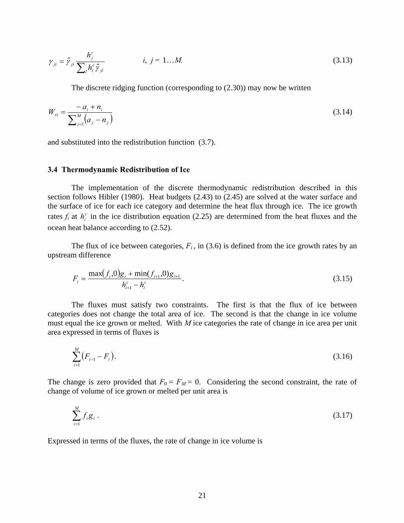
21
sum=
l jlcl
cj
jiji hh
γγγ
ˆˆ i j = 1hellipM (313)
The discrete ridging function (corresponding to (230)) may now be written
( )sum =minus
+minus= M
j jj
iiri
na
naW
1
(314)
and substituted into the redistribution function (37)
34 Thermodynamic Redistribution of Ice
The implementation of the discrete thermodynamic redistribution described in this
section follows Hibler (1980) Heat budgets (243) to (245) are solved at the water surface and the surface of ice for each ice category and determine the heat flux through ice The ice growth rates fi at c
ih in the ice distribution equation (225) are determined from the heat fluxes and the ocean heat balance according to (252)
The flux of ice between categories Fi in (36) is defined from the ice growth rates by an
upstream difference
( ) )0min(0max
1
11ci
ci
iiiii hh
gfgfFminus
+=
+
++ (315)
The fluxes must satisfy two constraints The first is that the flux of ice between
categories does not change the total area of ice The second is that the change in ice volume must equal the ice grown or melted With M ice categories the rate of change in ice area per unit area expressed in terms of fluxes is
( )sum=
minus minusM
iii FF
11 (316)
The change is zero provided that F0 = FM = 0 Considering the second constraint the rate of change of volume of ice grown or melted per unit area is
sum=
M
iii gf
1 (317)
Expressed in terms of the fluxes the rate of change in ice volume is
22
( )sum=
minus minusM
i
ciii hFF
11
( )summinus
=+ minus=
1
11
M
i
ci
cii hhF
( ) ( )[ ]summinus
=+++=
1
111 )0min0max
M
iiiii gfgf (318)
( ) ( )summinus
=
++=1
20min0max
M
iMMiiii gfgfgf
(317) and (318) are equal except in the case of f1 negative (open water is absorbing heat) and the case of fM positive (ice from the thickest category is growing) The fluxes Fi in (315) must then be modified to account for these two cases in addition to the requirements following (316)
Open Water Absorbing Heat
In the case of open water absorbing heat we specify that the heat is mixed under the ice and contributes to melt at the bottom surface of the ice We modify the rates of change of ice thickness to if prime
( )⎩⎨⎧
gtminus+=
=prime1110
1 iAfAfi
fi
i (319)
where A is the total ice concentration Note that (319) preserves the net rate of ice growth
sumsum==
=primeM
iiii
M
ii gfgf
11 (320)
Growth of Thickest Ice Category
The second case in which flux of the form (315) does not balance the change in ice volume is when the thickest ice is growing In this case we add thick ice growth proportionally to all ice categories Let
hgfC MM=1 (321)
Then define the flux
23
⎩⎨⎧
gt=minus
=1
1
1
1 igC
iACF
iithick (322)
The flux (322) has the property that the increase of ice area is balanced by a decrease in
open water area Note also that the total rate of increase in ice volume from Fthicki balances the rate of increase of volume from growth of the thickest ice category ie
MMci
M
iithick gfhF =sum
=2 (323)
Maximum Rate of Decay
Hibler (1980) suggests applying a maximum rate of ice decay (minimum growth rate) fmin taken here as minus015 m day-1 We modify the ice growth rates
( ) iimini gfff prime=primeprime max (324)
The difference between ii ff primeprimeprimeand represents excess heat which melts ice laterally The excess rate of decay is
( ) i
M
iii gffExcess sum
=
primeminusprimeprime=1
(325)
Similarly to the thick ice growth we allocate this decay proportionately to all ice categories Define
hExcessC =2 (326)
then the lateral melt in terms of a flux is
⎩⎨⎧
gtminus=
=1
1
2
2 igC
iACF
iilateral (327)
The redistribution of ice from growth or melt can be finally written as
ithickilateraliii FFFF
tg
1 ++minus=Δ
Δminus (328)
24
4 Canadian East Coast Ocean Model (CECOM)
The region of interest for the model extends from the Gulf of Maine in the south to Baffin Bay in the north The model is implemented on a spherical coordinate system To reduce the impact of converging meridians we select a spherical coordinate system that is rotated relative to the earthrsquos longitude and latitude so that the equator of the rotated system bisects the domain In the following sub-sections the coordinate transformation and model domain are described
41 Rotated Spherical Coordinates
The relation between Cartesian coordinates (x y z) and longitude and colatitude (φ θ) (refer to Figure 41) is x = sinθ cosφ y = sinθ sinφ (41) z = cosθ where we take the radius of the sphere as unity Consider the transformation from original coordinates r to coordinates in a rotated system rprime
⎟⎟⎟
⎠
⎞
⎜⎜⎜
⎝
⎛=
zyx
r rArr ⎟⎟⎟
⎠
⎞
⎜⎜⎜
⎝
⎛
primeprime=prime
zyx
r (42)
A rotated system can be defined by the successive application of three rotations (Figure 42) 1 angle ξ about the z axis 2 angle η about the new y axis and 3 angle ζ about the new z axis The angle of rotation is in the clockwise direction looking in the direction of the axis The transformations from r to rprime and components of vectors are given in Appendix 2
25
Figure 41 Spherical coordinate system with longitude φ and co-latitude θ
Figure 42 The decomposition of a coordinate system rotation into three successive rotations of ξ η and ζ The red line is the y axis after one rotation 42 The CECOM Domain
The CECOM model grid has a resolution of 01deg times 01deg As noted it is defined on a rotated spherical coordinate system (Figure 43) The model domain in the geography
26
coordinates and the inner and outer boundaries are shown in Figure 44 The bathymetry of the domain is drawn in Figure 45 Specifics of the domain are given in Table 41
Generalised sigma coordinates are used to retain near-surface resolution even as bottom
depth increases The procedure we use to select the vertical levels is somewhat arbitrary For sufficiently deep water (bottom depth greater than or equal to H1) we specify that a fixed upper layer and the underlying ocean each have a given number of levels The levels are scaled according to the fixed upper or varying lower layer thickness For shallow water (bottom depth less than or equal to H0) all levels are distributed uniformly Between H0 and H1 the levels are linearly interpolated between the levels for H0 and H1
H0 = 10 m H1 = 64 m and an upper layer thickness of 64 m are selected There are a
total of 21 levels with 8 levels in the upper layer and 13 levels in the underlying ocean (at depths greater than H1) These generalised coordinates are shown for a section across the Labrador shelf (27deg longitude in rotated coordinates) in Figure 46
Figure 43 CECOM grid defined by a rotated spherical coordinate system Lines of longitude and latitude in the rotated system are drawn in red
27
Figure 44 CECOM domain (green) in the geographic coordinates The double red lines are the inner and outer boundaries of the model The blue box is the boundary in the rotated system of Fig 43
28
Table 41 Specifications of the CECOM domain ________________________________________________________________________ Coordinate rotation ( ) )1718241( degminusdegdeg=ςηξ Extent (rotated coordinates) 0 to 40deg longitude minus11 to 103deg latitude Horizontal resolution 01deg times 01deg
Dimension 400 times 213 times 21 (east times north times vertical) 410 times 223 times 21 including boundary relaxation zones time step 450 s (internal) 15 s (external) ________________________________________________________________________
Figure 45 The bathymetry of the CECOM domain Depth contours of 200 1000 2000 hellip m are drawn Specified transports (Sv) at open ocean boundary are indicated
29
Figure 46 A cross-section of the generalized coordinates across the Labrador Shelf The upper panel shows the coordinates over the upper 200 m 43 Ocean Initial State Boundary Conditions and Model Spin-up
Monthly climatological ocean temperature and salinity are used as an initial state and as open ocean boundary conditions The monthly climatologies were obtained from an objective analysis of historical data archived at Bedford Institute of Oceanography (Tang 2007) The database covers an area from northern Baffin Bay to Cape Hatteras and from the coast to 42deg W It is derived from a variety of sources dating back to 1910 The objective analysis employed an iterative difference correction procedure with topography-dependent radii of influence The grid resolution is 16deg times 16deg Figure 47 is a sample plot from the data set showing surface temperature and salinity for September
30
Figure 47 Surface temperature and salinity for September from objective analysis The red dots are the locations of the raw data
31
Transports based on large-scale models and observations are specified at the open boundaries of the model (Clarke1983 Ezer and Mellor 1994) In the present implementation the transports as shown in Figure 45 are used Different specifications are being tested to obtain best results The vertical profile of normal velocity is determined by the density through the geostrophic relation The sea level elevation at the open boundaries is determined by geostrophy to within a constant
The model open ocean boundary (double red lines in Fig 44) is interrupted by land masses The procedure to determine sea level in the ocean straits (Nares Strait Lancaster Sound Jones Sound Hudson Strait and St Lawrence Estuary) is as follows We spin up the model with three diagnostic runs of 10 days duration each with zero wind stress The sea level at open boundaries of straits is set to the adjacent interior value from the end of the previous run The spin-up concludes with a 10-day prognostic run
The initial state consists of September temperature and salinity and zero ice We create
12 open ocean boundary conditions corresponding to the monthly temperature and salinity fields As noted previously the geostrophic relation determines sea level elevation only to within a constant The constants ie the sea level average across open boundaries in straits are determined from the spin-up The monthly boundary conditions are linearly interpolated to daily values The sea level elevation and transport stream function after the spin-up process are drawn in Figure 48
Figure 48 The sea level elevation (left) and transport stream function (right) following the spin-up process
32
44 Ice categories
The ice model is implemented with 10 ice thickness categories with boundaries at 005 018 038 066 106 158 224 304 398 and 504 m The corresponding central thicknesses c
ih are 0 012 028 052 086 132 191 254 351 and 451 m 5 Model Physics of WaveWatch III (WW3)
The WAVEWATCH III (hereafter WW3) wave model (version 222) is used in the BIO forecasting system to forecast wave height and direction This is a WAM-type ocean surface wave model developed at NOAANCEP (Tolman and Chalikov1996 Tolman 2002) It has been successfully applied in global and regional scale studies in many areas including the North Atlantic and has proven to be an effective tool to study wave spectral evaluation air-sea interactions and nonlinear wave-wave interactions WW3 is a discrete spectra and phase-averaged model (Battjes 1994)
For regional and global applications the directional wave spectrum is resolved at each model grid point in terms of wavenumber-direction bands and the evolution of the wave field is found by numerically solving the spectral wave action balance equation which is usually written as
σθ
θλ
λθφ
φφSNNk
kNN
tN
g =partpart
+partpart
+partpart
+partpart
+partpart ampampampamp cos
cos1 (5-1)
where λ is longitude φ is latitude θ is wave propagation direction k is wave number t is time σ is the intrinsic angular frequency WW3 evaluates the balance equation for the wave action spectrum )( txkN θ which is usually expressed in spherical coordinates (Komen et al 1994)
The derivatives in (5-1) are the propagation velocities in physical and spectral domains
RUcg φθ
φ+
=cosamp
φθ
λ λ
cossinR
Ucg +=amp
Rcg
g
θφθθ
costanminus= ampamp R is the radius of the earth and
φU and λU are current components in φ and λ directions The left side of equation (1) represents the local rate of change of wave action density propagation in physical space action density shifting in frequency and direction due to the spatial and temporal variation in depth and current The net source term S consists of wind input( inS )white-capping dissipation( dsS ) nonlinear wave-wave interactions( nlS ) and bottom friction( botS ) WW3 uses an explicit scheme to solve the action balance equation (1) for N
Two combinations of the source terms inS and dsS are available in WW3 The default set up of WW3 corresponds to the wave-boundary layer formulation for inS and dsS due to Tolman and Chalikov (1996) Tolman (2002) notes that application of this formulation has entailed a
33
correction in fetch-limited wave heights that results from atmospheric stratification which necessitates a re-tuning of the model by defining an lsquoeffectiversquo wind as well as an additional correction for the impact of stability on wave growth An alternate combination corresponds to WAM cycle 3 physics (hereafter denoted WAMC3 physics) in which inS and dsS are based on WAMDI (1988) Snyder et al (1981) and Komen et al (1994) Quadruplet nonlinear interactions nlS are simulated by DIA and bottom dissipation bfS by the JONSWAP parameterization of Hasselmann et al (1973) Padilla-Hernatildendez et al [2007] compared the WW3 model against WAM and SWAN models for two North Atlantic storms and found that WW3 provided the high quality statistical comparisons to deep water observations 6 The Bedford Institute Ocean Forecasting System (BIOFS) BIOFS is a real-time short-term (2-day) forecasting system for eastern Canadian waters The forecast period is constrained by input data from Environment Canada If meteorological data from long range weather forecasts are available the ocean forecasts can be extended to a longer period It consists of two sub-systems one for CECOM (Section 63) and one for WW3 (Section 64) Graphic display of the forecasts can be viewed at the following public website maintained by DFO httpwwwmardfo-mpogccascienceoceanicemodelice_ocean_forecasthtml The parameters displayed on the website are surface trajectories water level time series at selected locations ice concentration and thickness wave height and direction (Northwest Atlantic and Atlantic Maritimes) sea surface elevation (non-tidal) maps temperature at surface and 50 m They are given at hourly (water level time series) 6-hourly (wave) or 12-hourly (all others) intervals 61 Input Data Meteorological Data Meteorological forcing is taken from the Canadian Meteorological Centre (CMC) Global Environmental Multiscale (GEM) model (Mailhot et al 2006) which provides 48 hour forecasts twice daily at 0000 and 1200 UTC with fields output at 3 hour intervals The GEM model is an operational atmospheric model that is part of the Canadian Regional Forecast System (RFS) developed by Environment Canada The model uses a variable resolution grid over the entire globe with a mesoscale 15 km horizontal resolution window over Northern America Fields used in the forecasting system are 10m winds 2m air and dew point temperatures total cloud coverage and total accumulated precipitation All meteorological parameters are linearly interpolated to the ocean and wave model grids Except for the10 m winds the parameter values change every 3 hours For CECOM the 10m wind field is interpolated in time to the model time step of 75 minutes to avoid temporal discontinuities in the dynamical forcing Total accumulated
34
precipitation is converted to a precipitation rate For WW3 the wind fields are interpolated to the propagation time step of the respective wave model (see Section 64 for details) Sea-Ice Data Ice concentration data are used for data assimilation (Section 62) in the ice model and to define the wave domain in WW3 In WW3 a grid point is considered open ocean if the ice concentration is equal or less than 05 Otherwise it is considered land Digital sea ice charts which include ice concentration data are provided by Canadian Ice Services(CIS) Canadian waters are covered by five digital ice charts (Figure 61) Data from Eastern Arctic Hudson Bay and East Coast are used in the forecasting system CIS produces daily charts for the Gulf of StLawrence and the Labrador and Newfoundland coasts south of 58N Regional charts for Hudson Bay Baffin Bay and the Labrador coast north of 58N are produced fortnightly Typically the regional charts are released several days after the date for which they are valid Since these charts represent more of a two week average condition than an instantaneous one BIOFS uses a regional charts release date as its valid date
Figure 61 Coverage of CISrsquos digital ice charts (courtesy of CIS) The digital charts use the ldquoegg coderdquo (Environment Canada 2005) to indicate the sea ice partial concentration for each stage of development on a regularly spaced grid Each ldquoeggrdquo indicates up to three different ice types (ignoring trace amounts) each of which is assigned a stage and concentration The stage of development may be interpreted as an approximate
35
measure of the ice thickness The conversion of stage to ice model thickness category is illustrated in Table 61 There are also four special cases listed in Table 62 Table 61 Conversion from ice stage to ice model category
Ice stage of development Description
Ice model
categoryIce thickness
boundaries (m)
OW BW IF Open Water bergy water ice-free 1 -005 lt h le 005
1 New 2 005 lt h le 018
2 Nilas 2 005 lt h le 018
3 Young Unknown 3 018 lt h le 038
4 Young Grey 2 005 lt h le 018
5 Young Grey-White 3 018 lt h le 038
6 First Year Unknown 4 038 lt h le 066
7 First Year Thin 5 066 lt h le 106
8 First Year Thin First Stage 5 066 lt h le 106
9 First Year Thin Second Stage 5 066 lt h le 106
1 First Year Medium 6 106 lt h le 158
4 First Year Thick 7 158 lt h le 224
7 Old 8 224 lt h le 304
8 Old Second Year 9 304 lt h le 398
9 Old Multi-Year 9 304 lt h le 398
L Ice of Land Origin 9 304 lt h le 398
B Brash 3 018 lt h le 038
Each stage of development is first converted to a category The partial concentrations
and categories including flags (Table 62) are then nearest-neighbour interpolated to the model grid Grid points with land fast ice will be filled with neighbouring concentrations and categories Including flags in the interpolation preserves grid points which should not be filled by interpolation All the charts available for a forecast date are then combined Where charts overlap the concentrations of each category are averaged Flagged points are ignored in the averaging
36
Table 62 Interpolation of ice data
Ice stage of
development Description Action
POINT NOT COVERED BY
POLYGON Point is outside CIS analysis area Flag
LAND Land point Flag
ICEGLACE Useless CIS category indicating ice presence but not providing concentration or stage
Flag
FASTICE Land fast ice Nearest Neighbour
Tides Tidal constituents of elevation and velocity come from two sources Paturi et al (2008) provides eight constituents (M2 S2 N2 K2 K1 O1 P1 Q1) and covers most of the model domain up to Davis Strait Dunphy et al (2005) provides five tidal constituents (M2 S2 N2 K1 O1) for Baffin Bay Constituents are linearly interpolated to the model grid Where the two sources slightly overlap at Davis Strait matching constituents are averaged 62 Data assimilation in CECOM
Many assimilation schemes have been developed for oceanographic and meteorological applications in the past 20 years Advanced schemes such as 3-d and 4-d variational method and Karmen filter require massive resources and abundant data to yield optimum results In this section we describe three methods to assimilate the annual cycle of the temperature and salinity fields sea surface temperature and ice concentration data into the ocean forecast model Assimilation of the Annual Cycle of the Temperature and Salinity Fields Monthly temperature and salinity climatologies are prescribed at the open boundaries of CECOM Such constraints are not strong enough to prevent the temperature and salinity fields from drifting in multi-year integration To ensure the annual cycles are preserved a nudging term with a constant relaxation time scale tR of 45 days are added to the temperature and salinity equation
37
)(1 TTtt
TCLIM
R
minus+=partpart
)(1 SStt
SCLIM
R
minus+=partpart
where TCLIM and SCLIM are monthly temperature and salinity climatologies linearly interpolated to daily intervals Assimilation of Sea Surface Temperature Data Daily near real-time sea surface temperature (SST) derived mainly from satellite observations are provided by CMC The data are assimilated into the ocean forecast model using a flux correction method The method is based on the theory of optimal interpolation A correction term proportional to the differences between the modeled and observed SST is added to the heat flux equation
We first consider the equation for SST assimilation (see Appendix 4)
( ) [ ])()(
2exp)()( 2
2
22
2
om
ooo
om
mma tTtTtt
tTtT minus⎥⎥⎦
⎤
⎢⎢⎣
⎡ minusminus
++=
τεεε
(61)
where the superscripts and subscripts ldquoardquo ldquomrdquo and ldquoordquo in (61) denote ldquoassimilationrdquo ldquomodelrdquo and ldquoobservationrdquo respectively to is the time of the most recent observation and t is the model time 2
mε and 2oε are the model and data errors respectively τ is the correlation time scale of
SST Since change in SST ΔT is related to change in heat flux ΔQ by
Qhc
tT
p
d Δ=Δρ
where h is the mixed layer depth and td is the time interval of SST data the first terms on each side of (61) can be replaced by the corresponding heat fluxes The equation for SST data assimilation is
( ) [ ])()(2
exp)()( 2
2
om
ooo
d
pma tTtTtt
Ft
hctQtQ minus
⎥⎥⎦
⎤
⎢⎢⎣
⎡ minusminus+=
τρ
(62)
where F = 1 [1+ (εο εm)2] F ranges from 0 to 1 Not all parameters in (62) are well known To implement (62) in the forecast model the parameters are adjusted to yield optimal results
38
Figures 62 and 63 show the impact of data assimilation on model SST from a test run In this run F = 1 td = 1 day τ = 1 day were used and h = 20 m To reduce model noise in the run )( o
m tT in (62) was replaced by the model SST averaged over the previous day (from t0 - 1 day to t0) Significant improvements in the model SST can be achieved by using this assimilation scheme Without data assimilation the difference between the model and data at the Scotian Shelf is of the order of ~ 2o C The difference is reduced to a fraction of a degree with data assimilation Over the model domain the model without data assimilation over predicts SST in the northern Labrador Sea and under predicts SST in the coastal and the North Atlantic Current regions (Figs 63) Data assimilation is able to reduce the errors to less than 1o C
The SST assimilation is applied to ice free waters only In ice covered areas the sea
surface temperature is equal or very close to the freezing temperature
Figure 62 A comparison of SST in a 1o x 1o area centered at the indicated location with and without data assimilation
39
Figure 63 CMC SST (left) and the difference between the model and data with (middle) and without (right) data assimilation Assimilation of sea-ice data An insertion-nudging method is used for ice data assimilation Ice concentration data are inserted to the model gradually and the model concentration is restored to the data value with a prescribed time constant In the equation for the thickness distribution function a term proportional to the difference between the observed and values is introduced
( ) ( ))( ioi
iiice
i ggdiffusionhfg
gt
gminusΓ++Ψ=
partpart
+sdotnabla+part
partu (62)
where goi is the ice chart concentrations and gi is the model concentrations for ice of thickness category i Γ has the following form
⎥⎦
⎤⎢⎣
⎡ minusminus=Γ 2
2
2)(
expw
om
ttγ
γ (63)
where t is the model time to is the time for which the ice chart is valid γm and γw are adjustable parameters The Gaussian function in (63) limits nudging to the times around the ice chart time 1γm is the restoring time scale In the present implementation the values of 1γm and γw are set to 16 hours (5760 seconds) and 3 hours (10800 seconds) respectively At one hour from the ice chart time this scheme gives a concentration change rate of ~05 per hour At times plusmn 2γw from
40
the ice chart time the rate is negligible Where there is no ice chart data the nudging is not applied Figure 64 is a comparison of ice area south of 58o with and without data assimilation for January 2008 Figure 65 shows the ice concentration from CISrsquos East Coast ice chart and the model results with and without data assimilation The data assimilation significantly reduces the model error In particular ice cover in the Gulf of St Lawrence and the location of the eastern ice edge can be simulated more realistically with data assimilation
Figure 64 A comparison of the model ice area south of 58o N with (blue) and without (black) data assimilation The unit is percentage of the model area south of 58o N
41
Figure 65 Ice concentration for January 28 2008 data (left) model results without (middle) and with (right) data assimilation 63 Operational Implementation of CECOM The ice-ocean component of BIOFS is mostly comprised of MATLAB scripts that handle the pre-processing of model input fields the execution of the CECOM FORTRAN executable the post-processing of model results and the management of data files MATLAB was chosen for its platform independence interpolation and graphics functionalities and the abundance of open source tools such as M_Map (Pawlowicz 2006) readgrib (Blanton 2005) snctools (Evans 2007) and T_Tide (Pawlowicz et al 2002) Scheduling and automation is handled by the Linux bash shell but could easily be implemented for other platforms and operating systems Delivery of Meteorological and ice Data
As with any endeavor in real-time forecasting the primary concern is the timely delivery of the data required to force the forecast model To address this concern a separate subsystem written in bash shell scripts automates the retrieval of crucial meteorological forecast data transmitted from CMC to BIO server Emerald2 twice a day The subsystem polls the site for data and performs file checks after retrieval to verify file integrity There is usually a 5-6 hour delay between the CMC regional forecast and the appearance of the forecast data on their ftp site If the system fails to retrieve the data it retries for a predefined number of times The digital ice charts valid for 1800 UTC are delivered daily to an ftp server at BIO Starfish at ~2200 UTC The CIS delivery system itself checks for file integrity after delivery
42
Forecast Schedule CECOM is run three times daily within BIOFS producing 48 hour forecasts for 0000 and 1200 UTC (Table 63 Fig 66) Due to delays in receiving the meteorological data the CMC 1200 UTC data are received at ~1700-1800 UTC and the forecast completes at ~1800-1900 UTC A 1200 UTC data assimilation run using 1800 UTC sea ice concentration data and 1200 UTC sea surface temperature data (the same SST are received in the CMC 0000 UTC forecast data) is made the following morning at ~0300 UTC to assimilate the most recent ice chart and sea surface temperature data The 0000 UTC forecast is run four hours following the data assimilation run at ~0700 UTC Table 63 Ocean forecast schedule Both the local time ldquoATrdquo (Atlantic Time) and UTC are indicated
Day 1 Day 2
1 ndash 2 pm AT 2 ndash 3 pm AT 6 pm AT 11 pm AT 1 ndash 2 am AT 3 am AT
1700-1800 UTC 1800-1900 UTC 2200 UTC 0300 UTC 0500-0600 UTC 0700 UTC
CMC 1200 UTC forecast data
received
1200 UTC 48-hour forecast
CIS charts received
1200 UTC 48-hour ice
and SST assimilation
CMC 0000 UTC forecast data received
0000 UTC 48-hour forecast
43
Figure 66 Flow chart of the forecasting operations in a 24-hour period Forecast Methodology Each forecast is initialized with the most recent output of a previous forecast The ocean lateral boundary conditions are linearly interpolated to daily values from the monthly means to prevent discontinuity The boundary conditions also provide a constraint for temperature and salinity near the boundaries In the interior nudging and statistical interpolation are used to prevent long-term drifts and to assimilate sea surface temperature data into the model (see Section 62)
CMC 1200UTC data
CIS 1800UTC data
CMC 0000UTC data
12 UTC
forecast run
Data assim
ilation run
00 UTC
forecast run
1200 UTC forecasts
0000 UTC forecasts
Day 1 Day 2 Day 3
Ice concentration data
Sea surface temperature data
Add tide and Stokes drift
Add tide and Stokes drift
44
After the model run T_Tide (RPawlowicz et al 2002) calculates the tidal current and
elevation for the forecast period The tidal components are then linearly added to the forecast components For surface currents wave induced Stokes drifts are added to the model surface current to obtain the total surface current (Tang et al 2007) The Stokes drift us is obtained from the 2-dimensional wave spectrum E (f θ) of WW3 by integrations over frequency and direction
( )intint= θθπ dfdfEef kz
s 4 2ku (64)
where f is wave frequency θ is wave direction k is wave number and k is the magnitude of k
There are two options for the Strokes drift in the forecasting system us can be computed directly from (64) at every model grid point A simpler method is to parameterize us by surface winds us = a W + b W2 (65)
β = turning angle (positive for clockwise) relative to wind direction (66) where us and β are the magnitude and direction of us respectively and W is 10 m wind speed The parameters a b and β are determined from least-squared fits of the Strokes velocities computed from (64) for October-December 2007 In most applications (eg surface drifter floating object) vertically averaged surface currents are required The Stokes velocities in (65) and (66) are replaced vertically averaged Stokes velocities The results of the least-squared fits are given in Table 64 for different depths of averaging Table 64 Parameters values of the Stokes drift for different depths of averaging Depth (m) 1000a 1000b β (deg)
1 2525 0641 380 2 1656 0533 400 3 1176 0459 410 4 0889 0405 430 5 0699 0363 440
Drift tracks are calculated from the total surface current field Each track starts at a model grid point and is advected by the surface current Horizontal linear interpolation is used to calculate the surface current field between grid points Distances are calculated using the plane sailing method which ignores the earths curvature
45
For ice forecasts all available 1800 UTC ice charts from the previous day are processed and assimilated into the model to correct the model ice field as described in Section 62 For ocean forecasts 1200 UTC SST data from the previous day are assimilated into the model (Figure 66) 64 Operational Implementation of WW3
The wave models are implemented on a system of three nested grids (Figures 67 68 69 and Table 65) The spatial resolution increases from 10o in the coarse grid to 05o in the intermediate grid to 01667o (10rsquo) in the fine resolution grid This system of grids ensures that energy from distant storms is not lost in simulating storms making landfall in coastal areas of North America The grid dimensions and resolutions are given in Table 65 Etopo2 bathymetry is used from the United States National Geophysical Data Center at 2 minutes resolution WW3 is used for the coarse intermediate and fine resolution simulations Following the Courant-Friedrichs-Leacutevy (CFL) stability criterion the propagation time steps for WW3 are 20 and 10 minutes for the coarse and intermediate grids respectively and 4 minute propagation steps for the fine-resolution grid In Table 65 WW3 has 4 time steps Δtg is the global time step by which the entire wave model solution is propagated forward in time Δtρ1 is the maximum spatial (xy) propagation time step for the lowest frequency which is required to satisfy the CFL criterion Δtis is the maximum intra-spectral (k θ) propagation time step which is also required to satisfy the CFL criterion and Δtst is the minimum time step for the integration of the source terms which is dynamically adjusted for each grid and for Δtg
WW3 interpolates the wind fields to the propagation time step of the respective wave model For fast moving storms WW3 has a built-in scheme to reduce the source term integration time step when the situation is changing rapidly Moreover in WW3 the source term integration time step can be set by the user Thus we set the minimum source term time step to 5 minutes in the coarse-resolution grid to adequately simulate the storms considered here For the intermediate and fine grids source term time steps were both set to 25 (see Table 65) Details regarding the spectral range and resolution of the WW3 model are given in Table 66 in terms of the lowest and highest frequencies ( lowf and highf ) number of points ( n ) frequency resolution ( fΔ ) and angular resolutions ( θΔ ) The 48-hour WW3 wave forecasts run twice daily (0000 UTC and 1200UTC) WW3 simulates waves outside nearshore areas where shallow water wave processes are not important The model includes standard physics for wave propagation growth by wind nonlinear interactions dissipation due to whitecapping and dissipation due to bottom friction In coastal estuary and nearshore areas where water depth is shallow fine-resolution computational domains are sometimes needed for dedicated studies nested within coarserndashresolution basin-scale domains in order to resolve complex topography coastline features and shallow water wave physics In these special cases an option is that the shallow water SWAN wave model (version 4031) can be applied for a fourth domain nested within the third domain (Ris et al 1994 Booij et al 1996 Booij et al 1999 Holthuijsen et al 2003 Booij 2004) in these specific areas The physics of SWAN are different from that of WW3 especially for shallow water waves
46
SWAN can simulate shoaling refraction bottom friction and depth-induced wave breaking besides the processes for whitecapping wind input and nonlinear wave-wave interactions that are present in WW3 SWAN is formulated in terms of an action balance equation Xu et al (2007) describe the implementation of WW3 and nested grids for the North Atlantic and SWAN for Lunenburg Bay for studies related to the waves generated by hurricane Juan (September 28-29 2003)
Figure 67 Model domain of WW3 - Atlantic Ocean and sample model output (0600 UTC November 4 2007) The colors indicate significant wave height The arrows indicate wave period and direction
47
Figure 68 Model domain of WW3 ndash Northwestern North Atlantic Ocean and sample model output (0600 UTC November 4 2007) The colors indicate significant wave height The arrows indicate wave period and direction
48
Figure 69 Model domain of WW3 ndash Atlantic maritimes and sample model output (0600 UTC November 4 2007) The colors indicate significant wave height The arrows indicate wave period and direction
49
Table 65 Geographical location of the grids used in this study λ θΔ are the resolutions in longitude λ and latitudeφ and Nλ and Nφ are the number of points in λ and φ Finally tΔ is the propagation time step and tΔ ST is the required time step for source term integration for the three models as required to satisfy the CFL criterion GRIDS Longitude Latitude λ θΔ Nλ Nφ Δtg tΔ ST
Coarse 40oE ndash 82oW 75oSndash 77oN 1o 123 153 20 min 50 min
Intermediate 40oWndash75oW 20oN-75oN 05o 71 111 10 min 2min
Fine 47oWndash71oW 42oN-52oN 10rsquo 145 61 5 min 25 min
Table 66 Spectral domains for all models lowf highf are the default values
Parameters Value
lowf highf [s-1] 00418 06028
nf fΔ 29 11 ftimes
θn θΔ 36 10o
50
References Battjes JA 1994 Shallow water wave modelling Proc Int Symp Waves -Phys Numerical
Modelling University of British Columbia Vancouver I 1-23 Budyko MI 1974 Climate and Life Academic Press New York 508 pp Blanton B 2005 readgrib
httpwwwopnmlunceduOPNML_Matlabread_gribread_gribhtml Blumberg AF and GL Mellor 1987 A description of a three-dimensional coastal ocean
circulation model in Three-Dimensional Coastal Ocean Models Coastal Estuarine Sci 4 edited by NS Heaps pp 1-16 AGU Washington DC
Booij N LH Holthuijsen and RC Ris 1996 The ldquoSWANrdquo Wave Model For Shallow Water
Coastal Engineering 1 668~672
Booij N RC Ris and LH Holthuijsen 1999 A third-generation wave model for coastal regions Part I Model description and validation J Geophys Res 104 C4 7649-7666
Booij N 2004 SWAN Cycle III version 4041 user manual[Available online at httpfluidmechanicstudelftnlswanindexhtm]
Carton JA G Chepurin and X Cao 2000 A simple ocean data assimilation analysis of the
global upper ocean 1950-95 Part I methodology J Phys Oceanogr 30 294-309 Charnock H 1955 Wind stress on a water surface Quarterly Journal of Royal Meteorological
Society 81 pp 639ndash640 Clarke RA 1984 Transport through the Cape Farewell-Flemish Cap section Rapp PV Reun
Cons Int Explor Mer 185 120-130 Dunphy M F Dupont C G Hannah D Greenberg 2005 Validation of a modelling system for
tides in the Canadian Arctic Archipelago Can Tech Rep Hydrogr Ocean Sci 243 vi + 70 pp
Dunlap E BM Detracey and CL Tang 2007 Short-wave radiation and sea ice in Baffin Bay
Atmosphere-Ocean 45 195-210 Environment Canada 2005 ldquoMANICE - Manual of Standard Procedures for Observing and
Reporting Ice Conditionsrdquo httpice-glacesecgcca AppWsvPageDspcfmLang=engamplnid=23ampScndLvl=noampID=172
Evans J 2007 snctools httpmexcdfsourceforgenet
51
Ezer T and GL Mellor 1994 Diagnostic and prognostic calculations of the North Atlantic circulation and sea level using a sigma coordinate ocean model J Geophys Res 99 14159-14171
Flato GM 1994 McPIC Documentation for the multi-category particle-in-cell sea ice model
Can Tech Rep Hydrogr Ocean Sci 158 74 pp Gill AE 1982 Atmosphere-Ocean Dynamics Academic Press New York 662 pp Hasselmann K TP Barnett E Bouws H Carlson DE Cartwright K Enke JI Ewing H
Gienapp DE Hasselmann P Kruseman A Meerbrug P Muumlller DJ Olbers K Richter W Sell and H Walden 1973 Measurements of wind-wave growth and swell decay during the Joint North Sea Wave Project (JONSWAP) Dtsch Hydrogr Z A8(12) 95 pp
Hibler WD 1979 A dynamic thermodynamic sea ice model J Phys Oceanogr 9 815-846 Hibler WD 1980 Modeling a variable thickness sea ice cover Mon Wea Rev 108 1943-
1973 Holthuijsen L H and HN Booij 2003 Phase-decoupled refraction-diffraction for spectral
wave models Coastal Engineering 49 291-305 Jerlov NG 1968 Optical Oceanography 194 pp Elsevier Komen G J LCavaleri M Donelan M Hasselmann S Hasselmann P A E M Janssen
1994 Dynamics and Modeling of Ocean Waves Cambridge University Press 520pp Mailhot J S Beacutelair L Lefaivre B Bilodeau M Desgagneacute C Girard A Glazer A-M Leduc
A Meacutethot A Patoine A Plante A Rahill T Robinson D Talbot A Tremblay P Vaillancourt A Zadra A Qaddouri 2006 The 15-km Version of the Canadian Regional Forecast System Atmos-Ocean 44 133-149 DOI 103137ao440202
Martinsen EA and H Engedahl 1987 Implementation and testing of a lateral boundary
scheme as an open boundary condition in a barotropic ocean model Coastal Eng 11 603-627
Mellor GL and AF Blumberg 1985 Modeling vertical and horizontal diffusivities with the
sigma coordinate system Mon Wea Rev 113 1380-1383 Mellor GL and LH Kantha 1989 An ice-ocean coupled model J Geophys Res 94
10937-10954 Mellor GL and T Ezer 1991 A Gulf Stream model and an altimetry assimilation scheme J
Geophys Res 96 8779-8795
52
Mellor GL S Hakkinen T Ezer and R Patchen 2002 A generalization of a sigma coordinate ocean model and an intercomparison of model vertical grids in Ocean Forecasting Conceptual Basis and Applications edited by N Pinardi and J Woods pp 55-72 Springer Berlin
Mellor GL and AF Blumberg 2004 Wave breaking and ocean surface layer thermal
response J Phys Oceanogr 34 693-698 Padilla-Hernatildendez R W Perrie B Toulany and P C Smith 2007 Intercomparison of third
generation wave models Weather and Forecasting Vol 22 No 6pages 1229-1242 Parkinson C L and W M Washington 1979 A large-scale numerical model of sea ice J
Geophys Res 84 311-337 Paturi S G Han and B deYoung 2008 A 3-D multi-constituent data assimilative tidal model
of the northwest Atlantic Atmosphere-Ocean Submitted Paulson CL and JJ Simpson 1977 Irradiance measurements in the upper ocean J Phys
Oceangr 7 952-956 Pawlowicz R 2006 M_Map httpwwweosubcca~rich Pawlowicz R B Beardsley and S Lentz 2002 Classical tidal harmonic analysis including
error estimates in MATLAB using T_TIDE Computers and Geosciences 28 929-937 httpwwweosubcca~rich
Perrie W Gunther H Rosenthal W and Toulany B 1989 Modelling wind - generated
surface gravity waves using similarity Quart J Roy Met Soc 115 1373-1396 Ris RC Holthuijsen LH and Booij N 1994 A Spectral Model for Waves in the Near shore
Zone Coastal Engineering 1 68~78 Semtner AJ 1976 A model for the thermodynamic growth of sea ice in numerical
investigations of climate J Phys Oceanogr 67 379-389 Shine KP 1984 Parameterization of the shortwave flux over high albedo surfaces as a
function of cloud thickness and surface albedo Q J R Meterol Soc 110 747-764 Sloslashrdal LH EA Martinsen and AF Blumberg 1994 Modeling the response of an idealized
coastal ocean to a traveling storm and to flow over bottom topography J Phys Oceanogr 24 1698-1705
Smith SD 1988 Coefficients for sea surface wind stress heat flux and wind profiles as a
function wind speed and temperature J Geophys Res 93 15467-15472
53
Smith SD and FW Dobson 1984 The heat budget at Ocean Weather Station Bravo Atmos-Ocean 22 1-22
Snyder RL FW Dobson JA Elliot and RB Long 1981 Array measurements of
atmospheric pressure fluctuations above surface gravity waves J Fluid Mech 20 1166-1174
Tang CL 2007 High-resolution monthly temperature and salinity climatologies for the
northwestern North Atlantic Ocean Canadian Data Report of Hydrography and Ocean Sciences No 169 iv + 55 pp
Tang CL Q Gui and I Peterson 1996a Modeling the mean circulation of the Labrador Sea
and the adjacent shelves J Phys Oceangr 26 1989-2010 Tang CL and Q Gui 1996b A dynamical model for wind-driving ice modtion ndash applicaton to
ice drift on the Labrador Shelf J Geophys Res 101 28343-28364 Tang CL CK Ross T Yao B Petrie BM Detracey and E Dunlap 2004 The circulation
water masses and sea ice of Baffin Bay Progress of Oceanography 63 183-228 Tang CL W Perrie AD Jenkins BM Detracey Y Hu B Toulany and PC Smith 2007
Observation and modeling of surface currents on the Grand Banks a study of the wave effects on surface currents J Geophys Res 112 C10025 doi1010292006JC004028
Thorndike AS DA Rothrock GA Maykut and R Colony 1975 The thickness distribution
of sea ice J Geophys Res 80 4501-4513 Tolman H L 2002 User manual and system documentation of WAVEWATCH-III version
222 Technical Note [Available online at httppolarncepnoaagovwaves] Tolman H L and Chalikov DV 1996 Source terms in a third-generation wind-wave model J
Phys Oceanogr 26 2497-2518 WAMDI group 1988 The WAM model ndash a third generation ocean wave prediction model J
Phys Oceanogr 18 1775-1810 Xu F W Perrie B Toulany and P C Smith 2007 Wind-generated waves in Hurricane Juan
Ocean Modelling Vol 16 pages 188ndash205 Yao T CL Tang and IK Peterson 2000 Modeling the seasonal variation of sea ice in the
Labrador Sea with a coupled multi-category ice model and the Princeton Ocean Model J Geophys Res 105 1153-1165
Yao T CL Tang 2003 The formation and maintenance of the North Water Atmosphere-
Ocean 41 187-201
54
Zhang J and WD Hibler 1997 On an efficient numerical method for modeling sea ice dynamics J Geophys Res 102 8691-8702
55
Appendix 1 Turbulence closure
This appendix outlines the calculations of the vertical mixing coefficients from turbulence closure Governing equations for turbulence kinetic energy q22 and turbulence macroscale l are
)(222 2
1
322
22222
qAlB
qz
Kgzv
zuK
zqK
zzqw
yqv
xqu
tq
HHo
M
q
nablasdotnabla+minuspartpart
+⎥⎥⎦
⎤
⎢⎢⎣
⎡⎟⎠⎞
⎜⎝⎛
partpart
+⎟⎠⎞
⎜⎝⎛
partpart
+
⎟⎟⎠
⎞⎜⎜⎝
⎛part
partpartpart
=part
part+
partpart
+part
part+
partpart
ρρ
)(~ 2
1
31
22
1
22222
lqAwBq
zKglE
zv
zuKlE
zlqK
zzlqw
ylqv
xlqu
tlq
HHo
M
q
nablasdotnabla+minuspartpart
+⎥⎥⎦
⎤
⎢⎢⎣
⎡⎟⎠⎞
⎜⎝⎛
partpart
+⎟⎠⎞
⎜⎝⎛
partpart
+
⎟⎟⎠
⎞⎜⎜⎝
⎛part
partpartpart
=part
part+
partpart
+part
part+
partpart
ρρ
where
2
21~ ⎟⎠⎞
⎜⎝⎛+=
LlEw
κ
( ) ( ) 111 minusminusminus ++minus= zHzL η
κ is the von Karman constant and B1 E1 and E2 are empirical constants
The effects of wave breaking are taken into consideration through the surface boundary condition for q2 At the surface the vertical gradient of q2 is proportional to the cube of the water friction velocity (Mellor and Blumberg 2004) A consequence of this boundary condition is that the eddy viscosity is non-zero at the surface (Tang et al 2007) The boundary conditions at the surface are
⎪⎩
⎪⎨⎧
=
=part
partlowast
covered ice
free ice22
321
2
32
uBq
uz
qBCα
02 =lq
where αBC is a prescribed constant and u is the friction velocity
56
020
20
2 )( ρττ yxu +=
The boundary conditions at the ocean bottom are
02
2
321
2
=
=
lq
uBq
where u is derived from the bottom stress
The mixing coefficients KM KH and Kq can be expressed in terms of stability functions SM SH and Sq
)()( qHMqHM SSSlqKKK = The stability functions are derived from the solution of analytic equations (Blumberg and Mellor 1987) involving the vertical shear and vertical density gradient In the presence of ice the mixing coefficient is the average of the values for open ocean and for ice-covered ocean (no wave effects) weighted by ice concentration Appendix 2 Generalised sigma coordinates
Generalised sigma coordinates are derived by transforming coordinates (x y z t) to (x y s t) The vertical coordinate s is defined
)()( tyxtkyxsz η+= (A21) where s is a function of the vertical variable k which ranges from 1 at the surface to kb at the ocean bottom For the purposes of this discussion k is continuous but it is discrete for the computer implementation Since 0 =partpart xz then
0
xk
ks
xs
x partpart
partpart
+partpart
+partpart
=η
or
k
xx
ss
xk
η+
minus=partpart
Also the z derivative of (A21) gives
kszk 1
=partpart
57
For a function )( tzyxφ partial derivatives in the old coordinate system are related to partial derivatives in the new coordinate system as
1
k
tt
k
k
yy
k
xx
ss
ktt
skz
ss
kyy
ss
kxx
ηφφφ
φφ
ηφφφ
ηφφφ
+partpart
minuspartpart
=partpart
partpart
=partpart
+partpart
minuspartpart
=partpart
+partpart
minuspartpart
=partpart
We define a new vertical velocity ω as
( ) ( ) yyxxtt svsusw ηηηω ++++++=
The continuity equation in transformed coordinates (henceforth dropping the asterisks) is
0)()(
=partpart
+part
part+
partpart
+part
partky
vsx
ust
s kkk ω (A22)
The momentum equations in transformed coordinates are
( ) ( ) ( ) ( ) ( )
int int +⎟⎟⎠
⎞⎜⎜⎝
⎛partpart
partpart
+partpart
minuspartpart
+
+minus=minuspart
part+
partpart
+part
part+
partpart
xk
Mk
o
kx
o
k
xxkkkkk
Mku
sK
kdk
xsgsdk
ksgs
sgsfvsku
yuvs
xsu
tus
ρρ
ρρ
ηω 22
(A23)
( ) ( ) ( ) ( ) ( )
int int +⎟⎟⎠
⎞⎜⎜⎝
⎛partpart
partpart
+partpart
minuspartpart
+
+minus=+part
part+
partpart
+part
part+
partpart
yk
Mk
o
ky
o
k
yykkkkk
Mkv
sK
kdk
ysgsdk
ksgs
sgsfuskv
ysv
xuvs
tvs
ρρ
ρρ
ηω 22
(A24)
The heat and salt equations in transformed coordinates are
( ) ( ) ( ) ( )
Tk
Hkkk MkT
sK
kkT
yvTs
xuTs
tTs
+⎟⎟⎠
⎞⎜⎜⎝
⎛partpart
partpart
=part
part+
partpart
+part
part+
partpart ω
58
( ) ( ) ( ) ( )S
k
Hkkk MkS
sK
kkS
yvSs
xuSs
tSs
+⎟⎟⎠
⎞⎜⎜⎝
⎛partpart
partpart
=part
part+
partpart
+part
part+
partpart ω
The horizontal mixing terms become
⎥⎦
⎤⎢⎣
⎡⎟⎟⎠
⎞⎜⎜⎝
⎛partpart
+partpart
partpart
+⎟⎠⎞
⎜⎝⎛
partpart
partpart
=xv
yuAs
yxuAs
xM MkMkx 2
⎥⎦
⎤⎢⎣
⎡⎟⎟⎠
⎞⎜⎜⎝
⎛partpart
+partpart
partpart
+⎟⎟⎠
⎞⎜⎜⎝
⎛partpart
partpart
=xv
yuAs
xyvAs
yM MkMky 2
⎟⎟⎠
⎞⎜⎜⎝
⎛partpart
partpart
+⎟⎠⎞
⎜⎝⎛
partpart
partpart
=yTAs
yxTAs
xM HkMkT
⎟⎟⎠
⎞⎜⎜⎝
⎛partpart
partpart
+⎟⎠⎞
⎜⎝⎛
partpart
partpart
=ySAs
yxSAs
xM HkMkS
These forms are not simply the transformations of (28) This relates to separating vertical mixing from horizontal mixing in a coordinate system in which constant k surfaces are sloping (Mellor and Blumberg 1985 and Mellor et al 2002) Appendix 3 Rotated spherical coordinate system
Coordinates r on a unit sphere are transformed to rprime in a rotated system (42) with the matrix R by
rRRRRrr ξης==prime (A31) where Rξ Rη Rζ are transformation matrices for rotations by the individual angles ξ η and ζ respectively (Figure 42)
The individual rotation matrices are
⎟⎟⎟
⎠
⎞
⎜⎜⎜
⎝
⎛minus=
1000cossin0sincos
ξξξξ
ξR ⎟⎟⎟
⎠
⎞
⎜⎜⎜
⎝
⎛ minus=
ηη
ηη
η
cos0sin010
sin0cosR
⎟⎟⎟
⎠
⎞
⎜⎜⎜
⎝
⎛minus=
1000cossin0sincos
ςςςς
ςR (A32)
giving the matrix R as
59
⎟⎟⎟
⎠
⎞
⎜⎜⎜
⎝
⎛+minusminusminus
minus+minus
ηξηξηηςξςξηςξςξηςηςξςξηςξςξης
cossinsincossinsinsincoscossincossinsincoscoscossinsincoscossinsincoscossinsincoscoscos
(A33)
As well as transforming coordinates it is also necessary to transform components of
vectors tangent to the sphere Define α(φθ) as the angle between parallels of latitude (Figure A31) The angle between a vector and the local parallel in the rotated system is the corresponding angle in the original system minus α Denoting longitude and co-latitude in the rotated coordinate system as ( )θφ primeprime then
θφφφθα
sintanprimepartpart
primepartpartminus= (A34)
From (41) (φ θ) are related to (x y z) by tan φ = yx cosθ = z (A35)
The partial derivatives in (A34) may be written as
( ) 212
1
1cosz
zzminus
primepartpartminus=
primepartpart
=primepart
part minus φφφ
θ (A36)
and
( ) ⎟⎟⎠
⎞⎜⎜⎝
⎛primepart
partminus
primepartpart
+=
primepartpart
=primepart
part minus
φφφφφ xyyx
yxxy 22
1 1tan (A37)
Eqs (A36) and (A37) involve derivatives φprimepartpartr From (A31)
⎟⎟⎟
⎠
⎞
⎜⎜⎜
⎝
⎛
primeprimeprimeprimeprime
=⎟⎟⎟
⎠
⎞
⎜⎜⎜
⎝
⎛
primeprimeprime
=⎟⎟⎟
⎠
⎞
⎜⎜⎜
⎝
⎛minusminus
θφθφθ
cossinsincossin
11 RRzyx
zyx
(A38)
The partial derivatives in (A36) and (A37) are then
⎟⎟⎟
⎠
⎞
⎜⎜⎜
⎝
⎛primeprimeprimeprimeminus
=⎟⎟⎟
⎠
⎞
⎜⎜⎜
⎝
⎛
primepartpart
primepartpart
primepartpartminus
0cossinsinsin
1 φθφθ
φφφ
Rzyx
(A39)
60
We obtain α by substituting (A39) into (A36) and (A37) and then substituting (A36) and (A37) into (A34)
Figure A31 The angle α between a parallel of latitude in the rotated coordinate system and a parallel of latitude in the original system enables the transformation of components of a vector Appendix 4 Two-dimensional statistical interpolation Consider a variable Ti at a model time and grid point denoted by the subscript i The model value m
iT is corrected by past or present observations to yield an assimilated value aiT
according to
sum=
minus+=N
moi
mi
ai TTPTT
1)(
αααα (A4-1)
where oTα is the observation and mTα is the model value at the time and location of the observation denoted by the subscript ldquoαrdquo N is the number of observations to be included in the assimilation Piα are weights obtained by minimizing the difference between the model prediction and the observation which are solutions of the following algebraic equations (Mellor and Ezer 1991)
sum=
==+N
ii NMDMP1
21)(α
βαβαβα β (A4-2)
61
where Mαβ and Dαβ are the error matrices for model and observation respectively
oomm TTDTTM βααββααβ ΔsdotΔ=ΔsdotΔ= (A4-3)
mTαΔ and oTαΔ are the model and observation errors respectively The error matrices can be parameterized by a Gaussian and a delta function (Mellor and Ezer 1991 Carton et al 2000)
⎥⎥⎦
⎤
⎢⎢⎣
⎡ minusminus
minusminus
minusminus= 2
2
2
2
2
22
2)(
2)(
2)(
expxyx
m
ttL
yyLxx
Mτ
ε βαβαβααβ (A4-4)
αβαβ δε 2
oD = (A4-5) where Lx Ly and τ are the correlation scales of the model errors If the horizontal correlation scale is much larger than the grid spacing of the model the spatial part of (A4-4) can be neglected and (A4-1) is reduced to
)(2
)(exp 112
21
22
2moi
om
mmi
ai TT
ttTT minus⎥
⎦
⎤⎢⎣
⎡ minusminus
++=
τεεε
(A4-6)
where the subscript ldquo1rdquo denotes the time of the most recent observation ( itt le1 )
- Forecastsystem_18Nov08_Part_1
- Forecastsystem_10Dec08_Part_2
-

22
( )sum=
minus minusM
i
ciii hFF
11
( )summinus
=+ minus=
1
11
M
i
ci
cii hhF
( ) ( )[ ]summinus
=+++=
1
111 )0min0max
M
iiiii gfgf (318)
( ) ( )summinus
=
++=1
20min0max
M
iMMiiii gfgfgf
(317) and (318) are equal except in the case of f1 negative (open water is absorbing heat) and the case of fM positive (ice from the thickest category is growing) The fluxes Fi in (315) must then be modified to account for these two cases in addition to the requirements following (316)
Open Water Absorbing Heat
In the case of open water absorbing heat we specify that the heat is mixed under the ice and contributes to melt at the bottom surface of the ice We modify the rates of change of ice thickness to if prime
( )⎩⎨⎧
gtminus+=
=prime1110
1 iAfAfi
fi
i (319)
where A is the total ice concentration Note that (319) preserves the net rate of ice growth
sumsum==
=primeM
iiii
M
ii gfgf
11 (320)
Growth of Thickest Ice Category
The second case in which flux of the form (315) does not balance the change in ice volume is when the thickest ice is growing In this case we add thick ice growth proportionally to all ice categories Let
hgfC MM=1 (321)
Then define the flux
23
⎩⎨⎧
gt=minus
=1
1
1
1 igC
iACF
iithick (322)
The flux (322) has the property that the increase of ice area is balanced by a decrease in
open water area Note also that the total rate of increase in ice volume from Fthicki balances the rate of increase of volume from growth of the thickest ice category ie
MMci
M
iithick gfhF =sum
=2 (323)
Maximum Rate of Decay
Hibler (1980) suggests applying a maximum rate of ice decay (minimum growth rate) fmin taken here as minus015 m day-1 We modify the ice growth rates
( ) iimini gfff prime=primeprime max (324)
The difference between ii ff primeprimeprimeand represents excess heat which melts ice laterally The excess rate of decay is
( ) i
M
iii gffExcess sum
=
primeminusprimeprime=1
(325)
Similarly to the thick ice growth we allocate this decay proportionately to all ice categories Define
hExcessC =2 (326)
then the lateral melt in terms of a flux is
⎩⎨⎧
gtminus=
=1
1
2
2 igC
iACF
iilateral (327)
The redistribution of ice from growth or melt can be finally written as
ithickilateraliii FFFF
tg
1 ++minus=Δ
Δminus (328)
24
4 Canadian East Coast Ocean Model (CECOM)
The region of interest for the model extends from the Gulf of Maine in the south to Baffin Bay in the north The model is implemented on a spherical coordinate system To reduce the impact of converging meridians we select a spherical coordinate system that is rotated relative to the earthrsquos longitude and latitude so that the equator of the rotated system bisects the domain In the following sub-sections the coordinate transformation and model domain are described
41 Rotated Spherical Coordinates
The relation between Cartesian coordinates (x y z) and longitude and colatitude (φ θ) (refer to Figure 41) is x = sinθ cosφ y = sinθ sinφ (41) z = cosθ where we take the radius of the sphere as unity Consider the transformation from original coordinates r to coordinates in a rotated system rprime
⎟⎟⎟
⎠
⎞
⎜⎜⎜
⎝
⎛=
zyx
r rArr ⎟⎟⎟
⎠
⎞
⎜⎜⎜
⎝
⎛
primeprime=prime
zyx
r (42)
A rotated system can be defined by the successive application of three rotations (Figure 42) 1 angle ξ about the z axis 2 angle η about the new y axis and 3 angle ζ about the new z axis The angle of rotation is in the clockwise direction looking in the direction of the axis The transformations from r to rprime and components of vectors are given in Appendix 2
25
Figure 41 Spherical coordinate system with longitude φ and co-latitude θ
Figure 42 The decomposition of a coordinate system rotation into three successive rotations of ξ η and ζ The red line is the y axis after one rotation 42 The CECOM Domain
The CECOM model grid has a resolution of 01deg times 01deg As noted it is defined on a rotated spherical coordinate system (Figure 43) The model domain in the geography
26
coordinates and the inner and outer boundaries are shown in Figure 44 The bathymetry of the domain is drawn in Figure 45 Specifics of the domain are given in Table 41
Generalised sigma coordinates are used to retain near-surface resolution even as bottom
depth increases The procedure we use to select the vertical levels is somewhat arbitrary For sufficiently deep water (bottom depth greater than or equal to H1) we specify that a fixed upper layer and the underlying ocean each have a given number of levels The levels are scaled according to the fixed upper or varying lower layer thickness For shallow water (bottom depth less than or equal to H0) all levels are distributed uniformly Between H0 and H1 the levels are linearly interpolated between the levels for H0 and H1
H0 = 10 m H1 = 64 m and an upper layer thickness of 64 m are selected There are a
total of 21 levels with 8 levels in the upper layer and 13 levels in the underlying ocean (at depths greater than H1) These generalised coordinates are shown for a section across the Labrador shelf (27deg longitude in rotated coordinates) in Figure 46
Figure 43 CECOM grid defined by a rotated spherical coordinate system Lines of longitude and latitude in the rotated system are drawn in red
27
Figure 44 CECOM domain (green) in the geographic coordinates The double red lines are the inner and outer boundaries of the model The blue box is the boundary in the rotated system of Fig 43
28
Table 41 Specifications of the CECOM domain ________________________________________________________________________ Coordinate rotation ( ) )1718241( degminusdegdeg=ςηξ Extent (rotated coordinates) 0 to 40deg longitude minus11 to 103deg latitude Horizontal resolution 01deg times 01deg
Dimension 400 times 213 times 21 (east times north times vertical) 410 times 223 times 21 including boundary relaxation zones time step 450 s (internal) 15 s (external) ________________________________________________________________________
Figure 45 The bathymetry of the CECOM domain Depth contours of 200 1000 2000 hellip m are drawn Specified transports (Sv) at open ocean boundary are indicated
29
Figure 46 A cross-section of the generalized coordinates across the Labrador Shelf The upper panel shows the coordinates over the upper 200 m 43 Ocean Initial State Boundary Conditions and Model Spin-up
Monthly climatological ocean temperature and salinity are used as an initial state and as open ocean boundary conditions The monthly climatologies were obtained from an objective analysis of historical data archived at Bedford Institute of Oceanography (Tang 2007) The database covers an area from northern Baffin Bay to Cape Hatteras and from the coast to 42deg W It is derived from a variety of sources dating back to 1910 The objective analysis employed an iterative difference correction procedure with topography-dependent radii of influence The grid resolution is 16deg times 16deg Figure 47 is a sample plot from the data set showing surface temperature and salinity for September
30
Figure 47 Surface temperature and salinity for September from objective analysis The red dots are the locations of the raw data
31
Transports based on large-scale models and observations are specified at the open boundaries of the model (Clarke1983 Ezer and Mellor 1994) In the present implementation the transports as shown in Figure 45 are used Different specifications are being tested to obtain best results The vertical profile of normal velocity is determined by the density through the geostrophic relation The sea level elevation at the open boundaries is determined by geostrophy to within a constant
The model open ocean boundary (double red lines in Fig 44) is interrupted by land masses The procedure to determine sea level in the ocean straits (Nares Strait Lancaster Sound Jones Sound Hudson Strait and St Lawrence Estuary) is as follows We spin up the model with three diagnostic runs of 10 days duration each with zero wind stress The sea level at open boundaries of straits is set to the adjacent interior value from the end of the previous run The spin-up concludes with a 10-day prognostic run
The initial state consists of September temperature and salinity and zero ice We create
12 open ocean boundary conditions corresponding to the monthly temperature and salinity fields As noted previously the geostrophic relation determines sea level elevation only to within a constant The constants ie the sea level average across open boundaries in straits are determined from the spin-up The monthly boundary conditions are linearly interpolated to daily values The sea level elevation and transport stream function after the spin-up process are drawn in Figure 48
Figure 48 The sea level elevation (left) and transport stream function (right) following the spin-up process
32
44 Ice categories
The ice model is implemented with 10 ice thickness categories with boundaries at 005 018 038 066 106 158 224 304 398 and 504 m The corresponding central thicknesses c
ih are 0 012 028 052 086 132 191 254 351 and 451 m 5 Model Physics of WaveWatch III (WW3)
The WAVEWATCH III (hereafter WW3) wave model (version 222) is used in the BIO forecasting system to forecast wave height and direction This is a WAM-type ocean surface wave model developed at NOAANCEP (Tolman and Chalikov1996 Tolman 2002) It has been successfully applied in global and regional scale studies in many areas including the North Atlantic and has proven to be an effective tool to study wave spectral evaluation air-sea interactions and nonlinear wave-wave interactions WW3 is a discrete spectra and phase-averaged model (Battjes 1994)
For regional and global applications the directional wave spectrum is resolved at each model grid point in terms of wavenumber-direction bands and the evolution of the wave field is found by numerically solving the spectral wave action balance equation which is usually written as
σθ
θλ
λθφ
φφSNNk
kNN
tN
g =partpart
+partpart
+partpart
+partpart
+partpart ampampampamp cos
cos1 (5-1)
where λ is longitude φ is latitude θ is wave propagation direction k is wave number t is time σ is the intrinsic angular frequency WW3 evaluates the balance equation for the wave action spectrum )( txkN θ which is usually expressed in spherical coordinates (Komen et al 1994)
The derivatives in (5-1) are the propagation velocities in physical and spectral domains
RUcg φθ
φ+
=cosamp
φθ
λ λ
cossinR
Ucg +=amp
Rcg
g
θφθθ
costanminus= ampamp R is the radius of the earth and
φU and λU are current components in φ and λ directions The left side of equation (1) represents the local rate of change of wave action density propagation in physical space action density shifting in frequency and direction due to the spatial and temporal variation in depth and current The net source term S consists of wind input( inS )white-capping dissipation( dsS ) nonlinear wave-wave interactions( nlS ) and bottom friction( botS ) WW3 uses an explicit scheme to solve the action balance equation (1) for N
Two combinations of the source terms inS and dsS are available in WW3 The default set up of WW3 corresponds to the wave-boundary layer formulation for inS and dsS due to Tolman and Chalikov (1996) Tolman (2002) notes that application of this formulation has entailed a
33
correction in fetch-limited wave heights that results from atmospheric stratification which necessitates a re-tuning of the model by defining an lsquoeffectiversquo wind as well as an additional correction for the impact of stability on wave growth An alternate combination corresponds to WAM cycle 3 physics (hereafter denoted WAMC3 physics) in which inS and dsS are based on WAMDI (1988) Snyder et al (1981) and Komen et al (1994) Quadruplet nonlinear interactions nlS are simulated by DIA and bottom dissipation bfS by the JONSWAP parameterization of Hasselmann et al (1973) Padilla-Hernatildendez et al [2007] compared the WW3 model against WAM and SWAN models for two North Atlantic storms and found that WW3 provided the high quality statistical comparisons to deep water observations 6 The Bedford Institute Ocean Forecasting System (BIOFS) BIOFS is a real-time short-term (2-day) forecasting system for eastern Canadian waters The forecast period is constrained by input data from Environment Canada If meteorological data from long range weather forecasts are available the ocean forecasts can be extended to a longer period It consists of two sub-systems one for CECOM (Section 63) and one for WW3 (Section 64) Graphic display of the forecasts can be viewed at the following public website maintained by DFO httpwwwmardfo-mpogccascienceoceanicemodelice_ocean_forecasthtml The parameters displayed on the website are surface trajectories water level time series at selected locations ice concentration and thickness wave height and direction (Northwest Atlantic and Atlantic Maritimes) sea surface elevation (non-tidal) maps temperature at surface and 50 m They are given at hourly (water level time series) 6-hourly (wave) or 12-hourly (all others) intervals 61 Input Data Meteorological Data Meteorological forcing is taken from the Canadian Meteorological Centre (CMC) Global Environmental Multiscale (GEM) model (Mailhot et al 2006) which provides 48 hour forecasts twice daily at 0000 and 1200 UTC with fields output at 3 hour intervals The GEM model is an operational atmospheric model that is part of the Canadian Regional Forecast System (RFS) developed by Environment Canada The model uses a variable resolution grid over the entire globe with a mesoscale 15 km horizontal resolution window over Northern America Fields used in the forecasting system are 10m winds 2m air and dew point temperatures total cloud coverage and total accumulated precipitation All meteorological parameters are linearly interpolated to the ocean and wave model grids Except for the10 m winds the parameter values change every 3 hours For CECOM the 10m wind field is interpolated in time to the model time step of 75 minutes to avoid temporal discontinuities in the dynamical forcing Total accumulated
34
precipitation is converted to a precipitation rate For WW3 the wind fields are interpolated to the propagation time step of the respective wave model (see Section 64 for details) Sea-Ice Data Ice concentration data are used for data assimilation (Section 62) in the ice model and to define the wave domain in WW3 In WW3 a grid point is considered open ocean if the ice concentration is equal or less than 05 Otherwise it is considered land Digital sea ice charts which include ice concentration data are provided by Canadian Ice Services(CIS) Canadian waters are covered by five digital ice charts (Figure 61) Data from Eastern Arctic Hudson Bay and East Coast are used in the forecasting system CIS produces daily charts for the Gulf of StLawrence and the Labrador and Newfoundland coasts south of 58N Regional charts for Hudson Bay Baffin Bay and the Labrador coast north of 58N are produced fortnightly Typically the regional charts are released several days after the date for which they are valid Since these charts represent more of a two week average condition than an instantaneous one BIOFS uses a regional charts release date as its valid date
Figure 61 Coverage of CISrsquos digital ice charts (courtesy of CIS) The digital charts use the ldquoegg coderdquo (Environment Canada 2005) to indicate the sea ice partial concentration for each stage of development on a regularly spaced grid Each ldquoeggrdquo indicates up to three different ice types (ignoring trace amounts) each of which is assigned a stage and concentration The stage of development may be interpreted as an approximate
35
measure of the ice thickness The conversion of stage to ice model thickness category is illustrated in Table 61 There are also four special cases listed in Table 62 Table 61 Conversion from ice stage to ice model category
Ice stage of development Description
Ice model
categoryIce thickness
boundaries (m)
OW BW IF Open Water bergy water ice-free 1 -005 lt h le 005
1 New 2 005 lt h le 018
2 Nilas 2 005 lt h le 018
3 Young Unknown 3 018 lt h le 038
4 Young Grey 2 005 lt h le 018
5 Young Grey-White 3 018 lt h le 038
6 First Year Unknown 4 038 lt h le 066
7 First Year Thin 5 066 lt h le 106
8 First Year Thin First Stage 5 066 lt h le 106
9 First Year Thin Second Stage 5 066 lt h le 106
1 First Year Medium 6 106 lt h le 158
4 First Year Thick 7 158 lt h le 224
7 Old 8 224 lt h le 304
8 Old Second Year 9 304 lt h le 398
9 Old Multi-Year 9 304 lt h le 398
L Ice of Land Origin 9 304 lt h le 398
B Brash 3 018 lt h le 038
Each stage of development is first converted to a category The partial concentrations
and categories including flags (Table 62) are then nearest-neighbour interpolated to the model grid Grid points with land fast ice will be filled with neighbouring concentrations and categories Including flags in the interpolation preserves grid points which should not be filled by interpolation All the charts available for a forecast date are then combined Where charts overlap the concentrations of each category are averaged Flagged points are ignored in the averaging
36
Table 62 Interpolation of ice data
Ice stage of
development Description Action
POINT NOT COVERED BY
POLYGON Point is outside CIS analysis area Flag
LAND Land point Flag
ICEGLACE Useless CIS category indicating ice presence but not providing concentration or stage
Flag
FASTICE Land fast ice Nearest Neighbour
Tides Tidal constituents of elevation and velocity come from two sources Paturi et al (2008) provides eight constituents (M2 S2 N2 K2 K1 O1 P1 Q1) and covers most of the model domain up to Davis Strait Dunphy et al (2005) provides five tidal constituents (M2 S2 N2 K1 O1) for Baffin Bay Constituents are linearly interpolated to the model grid Where the two sources slightly overlap at Davis Strait matching constituents are averaged 62 Data assimilation in CECOM
Many assimilation schemes have been developed for oceanographic and meteorological applications in the past 20 years Advanced schemes such as 3-d and 4-d variational method and Karmen filter require massive resources and abundant data to yield optimum results In this section we describe three methods to assimilate the annual cycle of the temperature and salinity fields sea surface temperature and ice concentration data into the ocean forecast model Assimilation of the Annual Cycle of the Temperature and Salinity Fields Monthly temperature and salinity climatologies are prescribed at the open boundaries of CECOM Such constraints are not strong enough to prevent the temperature and salinity fields from drifting in multi-year integration To ensure the annual cycles are preserved a nudging term with a constant relaxation time scale tR of 45 days are added to the temperature and salinity equation
37
)(1 TTtt
TCLIM
R
minus+=partpart
)(1 SStt
SCLIM
R
minus+=partpart
where TCLIM and SCLIM are monthly temperature and salinity climatologies linearly interpolated to daily intervals Assimilation of Sea Surface Temperature Data Daily near real-time sea surface temperature (SST) derived mainly from satellite observations are provided by CMC The data are assimilated into the ocean forecast model using a flux correction method The method is based on the theory of optimal interpolation A correction term proportional to the differences between the modeled and observed SST is added to the heat flux equation
We first consider the equation for SST assimilation (see Appendix 4)
( ) [ ])()(
2exp)()( 2
2
22
2
om
ooo
om
mma tTtTtt
tTtT minus⎥⎥⎦
⎤
⎢⎢⎣
⎡ minusminus
++=
τεεε
(61)
where the superscripts and subscripts ldquoardquo ldquomrdquo and ldquoordquo in (61) denote ldquoassimilationrdquo ldquomodelrdquo and ldquoobservationrdquo respectively to is the time of the most recent observation and t is the model time 2
mε and 2oε are the model and data errors respectively τ is the correlation time scale of
SST Since change in SST ΔT is related to change in heat flux ΔQ by
Qhc
tT
p
d Δ=Δρ
where h is the mixed layer depth and td is the time interval of SST data the first terms on each side of (61) can be replaced by the corresponding heat fluxes The equation for SST data assimilation is
( ) [ ])()(2
exp)()( 2
2
om
ooo
d
pma tTtTtt
Ft
hctQtQ minus
⎥⎥⎦
⎤
⎢⎢⎣
⎡ minusminus+=
τρ
(62)
where F = 1 [1+ (εο εm)2] F ranges from 0 to 1 Not all parameters in (62) are well known To implement (62) in the forecast model the parameters are adjusted to yield optimal results
38
Figures 62 and 63 show the impact of data assimilation on model SST from a test run In this run F = 1 td = 1 day τ = 1 day were used and h = 20 m To reduce model noise in the run )( o
m tT in (62) was replaced by the model SST averaged over the previous day (from t0 - 1 day to t0) Significant improvements in the model SST can be achieved by using this assimilation scheme Without data assimilation the difference between the model and data at the Scotian Shelf is of the order of ~ 2o C The difference is reduced to a fraction of a degree with data assimilation Over the model domain the model without data assimilation over predicts SST in the northern Labrador Sea and under predicts SST in the coastal and the North Atlantic Current regions (Figs 63) Data assimilation is able to reduce the errors to less than 1o C
The SST assimilation is applied to ice free waters only In ice covered areas the sea
surface temperature is equal or very close to the freezing temperature
Figure 62 A comparison of SST in a 1o x 1o area centered at the indicated location with and without data assimilation
39
Figure 63 CMC SST (left) and the difference between the model and data with (middle) and without (right) data assimilation Assimilation of sea-ice data An insertion-nudging method is used for ice data assimilation Ice concentration data are inserted to the model gradually and the model concentration is restored to the data value with a prescribed time constant In the equation for the thickness distribution function a term proportional to the difference between the observed and values is introduced
( ) ( ))( ioi
iiice
i ggdiffusionhfg
gt
gminusΓ++Ψ=
partpart
+sdotnabla+part
partu (62)
where goi is the ice chart concentrations and gi is the model concentrations for ice of thickness category i Γ has the following form
⎥⎦
⎤⎢⎣
⎡ minusminus=Γ 2
2
2)(
expw
om
ttγ
γ (63)
where t is the model time to is the time for which the ice chart is valid γm and γw are adjustable parameters The Gaussian function in (63) limits nudging to the times around the ice chart time 1γm is the restoring time scale In the present implementation the values of 1γm and γw are set to 16 hours (5760 seconds) and 3 hours (10800 seconds) respectively At one hour from the ice chart time this scheme gives a concentration change rate of ~05 per hour At times plusmn 2γw from
40
the ice chart time the rate is negligible Where there is no ice chart data the nudging is not applied Figure 64 is a comparison of ice area south of 58o with and without data assimilation for January 2008 Figure 65 shows the ice concentration from CISrsquos East Coast ice chart and the model results with and without data assimilation The data assimilation significantly reduces the model error In particular ice cover in the Gulf of St Lawrence and the location of the eastern ice edge can be simulated more realistically with data assimilation
Figure 64 A comparison of the model ice area south of 58o N with (blue) and without (black) data assimilation The unit is percentage of the model area south of 58o N
41
Figure 65 Ice concentration for January 28 2008 data (left) model results without (middle) and with (right) data assimilation 63 Operational Implementation of CECOM The ice-ocean component of BIOFS is mostly comprised of MATLAB scripts that handle the pre-processing of model input fields the execution of the CECOM FORTRAN executable the post-processing of model results and the management of data files MATLAB was chosen for its platform independence interpolation and graphics functionalities and the abundance of open source tools such as M_Map (Pawlowicz 2006) readgrib (Blanton 2005) snctools (Evans 2007) and T_Tide (Pawlowicz et al 2002) Scheduling and automation is handled by the Linux bash shell but could easily be implemented for other platforms and operating systems Delivery of Meteorological and ice Data
As with any endeavor in real-time forecasting the primary concern is the timely delivery of the data required to force the forecast model To address this concern a separate subsystem written in bash shell scripts automates the retrieval of crucial meteorological forecast data transmitted from CMC to BIO server Emerald2 twice a day The subsystem polls the site for data and performs file checks after retrieval to verify file integrity There is usually a 5-6 hour delay between the CMC regional forecast and the appearance of the forecast data on their ftp site If the system fails to retrieve the data it retries for a predefined number of times The digital ice charts valid for 1800 UTC are delivered daily to an ftp server at BIO Starfish at ~2200 UTC The CIS delivery system itself checks for file integrity after delivery
42
Forecast Schedule CECOM is run three times daily within BIOFS producing 48 hour forecasts for 0000 and 1200 UTC (Table 63 Fig 66) Due to delays in receiving the meteorological data the CMC 1200 UTC data are received at ~1700-1800 UTC and the forecast completes at ~1800-1900 UTC A 1200 UTC data assimilation run using 1800 UTC sea ice concentration data and 1200 UTC sea surface temperature data (the same SST are received in the CMC 0000 UTC forecast data) is made the following morning at ~0300 UTC to assimilate the most recent ice chart and sea surface temperature data The 0000 UTC forecast is run four hours following the data assimilation run at ~0700 UTC Table 63 Ocean forecast schedule Both the local time ldquoATrdquo (Atlantic Time) and UTC are indicated
Day 1 Day 2
1 ndash 2 pm AT 2 ndash 3 pm AT 6 pm AT 11 pm AT 1 ndash 2 am AT 3 am AT
1700-1800 UTC 1800-1900 UTC 2200 UTC 0300 UTC 0500-0600 UTC 0700 UTC
CMC 1200 UTC forecast data
received
1200 UTC 48-hour forecast
CIS charts received
1200 UTC 48-hour ice
and SST assimilation
CMC 0000 UTC forecast data received
0000 UTC 48-hour forecast
43
Figure 66 Flow chart of the forecasting operations in a 24-hour period Forecast Methodology Each forecast is initialized with the most recent output of a previous forecast The ocean lateral boundary conditions are linearly interpolated to daily values from the monthly means to prevent discontinuity The boundary conditions also provide a constraint for temperature and salinity near the boundaries In the interior nudging and statistical interpolation are used to prevent long-term drifts and to assimilate sea surface temperature data into the model (see Section 62)
CMC 1200UTC data
CIS 1800UTC data
CMC 0000UTC data
12 UTC
forecast run
Data assim
ilation run
00 UTC
forecast run
1200 UTC forecasts
0000 UTC forecasts
Day 1 Day 2 Day 3
Ice concentration data
Sea surface temperature data
Add tide and Stokes drift
Add tide and Stokes drift
44
After the model run T_Tide (RPawlowicz et al 2002) calculates the tidal current and
elevation for the forecast period The tidal components are then linearly added to the forecast components For surface currents wave induced Stokes drifts are added to the model surface current to obtain the total surface current (Tang et al 2007) The Stokes drift us is obtained from the 2-dimensional wave spectrum E (f θ) of WW3 by integrations over frequency and direction
( )intint= θθπ dfdfEef kz
s 4 2ku (64)
where f is wave frequency θ is wave direction k is wave number and k is the magnitude of k
There are two options for the Strokes drift in the forecasting system us can be computed directly from (64) at every model grid point A simpler method is to parameterize us by surface winds us = a W + b W2 (65)
β = turning angle (positive for clockwise) relative to wind direction (66) where us and β are the magnitude and direction of us respectively and W is 10 m wind speed The parameters a b and β are determined from least-squared fits of the Strokes velocities computed from (64) for October-December 2007 In most applications (eg surface drifter floating object) vertically averaged surface currents are required The Stokes velocities in (65) and (66) are replaced vertically averaged Stokes velocities The results of the least-squared fits are given in Table 64 for different depths of averaging Table 64 Parameters values of the Stokes drift for different depths of averaging Depth (m) 1000a 1000b β (deg)
1 2525 0641 380 2 1656 0533 400 3 1176 0459 410 4 0889 0405 430 5 0699 0363 440
Drift tracks are calculated from the total surface current field Each track starts at a model grid point and is advected by the surface current Horizontal linear interpolation is used to calculate the surface current field between grid points Distances are calculated using the plane sailing method which ignores the earths curvature
45
For ice forecasts all available 1800 UTC ice charts from the previous day are processed and assimilated into the model to correct the model ice field as described in Section 62 For ocean forecasts 1200 UTC SST data from the previous day are assimilated into the model (Figure 66) 64 Operational Implementation of WW3
The wave models are implemented on a system of three nested grids (Figures 67 68 69 and Table 65) The spatial resolution increases from 10o in the coarse grid to 05o in the intermediate grid to 01667o (10rsquo) in the fine resolution grid This system of grids ensures that energy from distant storms is not lost in simulating storms making landfall in coastal areas of North America The grid dimensions and resolutions are given in Table 65 Etopo2 bathymetry is used from the United States National Geophysical Data Center at 2 minutes resolution WW3 is used for the coarse intermediate and fine resolution simulations Following the Courant-Friedrichs-Leacutevy (CFL) stability criterion the propagation time steps for WW3 are 20 and 10 minutes for the coarse and intermediate grids respectively and 4 minute propagation steps for the fine-resolution grid In Table 65 WW3 has 4 time steps Δtg is the global time step by which the entire wave model solution is propagated forward in time Δtρ1 is the maximum spatial (xy) propagation time step for the lowest frequency which is required to satisfy the CFL criterion Δtis is the maximum intra-spectral (k θ) propagation time step which is also required to satisfy the CFL criterion and Δtst is the minimum time step for the integration of the source terms which is dynamically adjusted for each grid and for Δtg
WW3 interpolates the wind fields to the propagation time step of the respective wave model For fast moving storms WW3 has a built-in scheme to reduce the source term integration time step when the situation is changing rapidly Moreover in WW3 the source term integration time step can be set by the user Thus we set the minimum source term time step to 5 minutes in the coarse-resolution grid to adequately simulate the storms considered here For the intermediate and fine grids source term time steps were both set to 25 (see Table 65) Details regarding the spectral range and resolution of the WW3 model are given in Table 66 in terms of the lowest and highest frequencies ( lowf and highf ) number of points ( n ) frequency resolution ( fΔ ) and angular resolutions ( θΔ ) The 48-hour WW3 wave forecasts run twice daily (0000 UTC and 1200UTC) WW3 simulates waves outside nearshore areas where shallow water wave processes are not important The model includes standard physics for wave propagation growth by wind nonlinear interactions dissipation due to whitecapping and dissipation due to bottom friction In coastal estuary and nearshore areas where water depth is shallow fine-resolution computational domains are sometimes needed for dedicated studies nested within coarserndashresolution basin-scale domains in order to resolve complex topography coastline features and shallow water wave physics In these special cases an option is that the shallow water SWAN wave model (version 4031) can be applied for a fourth domain nested within the third domain (Ris et al 1994 Booij et al 1996 Booij et al 1999 Holthuijsen et al 2003 Booij 2004) in these specific areas The physics of SWAN are different from that of WW3 especially for shallow water waves
46
SWAN can simulate shoaling refraction bottom friction and depth-induced wave breaking besides the processes for whitecapping wind input and nonlinear wave-wave interactions that are present in WW3 SWAN is formulated in terms of an action balance equation Xu et al (2007) describe the implementation of WW3 and nested grids for the North Atlantic and SWAN for Lunenburg Bay for studies related to the waves generated by hurricane Juan (September 28-29 2003)
Figure 67 Model domain of WW3 - Atlantic Ocean and sample model output (0600 UTC November 4 2007) The colors indicate significant wave height The arrows indicate wave period and direction
47
Figure 68 Model domain of WW3 ndash Northwestern North Atlantic Ocean and sample model output (0600 UTC November 4 2007) The colors indicate significant wave height The arrows indicate wave period and direction
48
Figure 69 Model domain of WW3 ndash Atlantic maritimes and sample model output (0600 UTC November 4 2007) The colors indicate significant wave height The arrows indicate wave period and direction
49
Table 65 Geographical location of the grids used in this study λ θΔ are the resolutions in longitude λ and latitudeφ and Nλ and Nφ are the number of points in λ and φ Finally tΔ is the propagation time step and tΔ ST is the required time step for source term integration for the three models as required to satisfy the CFL criterion GRIDS Longitude Latitude λ θΔ Nλ Nφ Δtg tΔ ST
Coarse 40oE ndash 82oW 75oSndash 77oN 1o 123 153 20 min 50 min
Intermediate 40oWndash75oW 20oN-75oN 05o 71 111 10 min 2min
Fine 47oWndash71oW 42oN-52oN 10rsquo 145 61 5 min 25 min
Table 66 Spectral domains for all models lowf highf are the default values
Parameters Value
lowf highf [s-1] 00418 06028
nf fΔ 29 11 ftimes
θn θΔ 36 10o
50
References Battjes JA 1994 Shallow water wave modelling Proc Int Symp Waves -Phys Numerical
Modelling University of British Columbia Vancouver I 1-23 Budyko MI 1974 Climate and Life Academic Press New York 508 pp Blanton B 2005 readgrib
httpwwwopnmlunceduOPNML_Matlabread_gribread_gribhtml Blumberg AF and GL Mellor 1987 A description of a three-dimensional coastal ocean
circulation model in Three-Dimensional Coastal Ocean Models Coastal Estuarine Sci 4 edited by NS Heaps pp 1-16 AGU Washington DC
Booij N LH Holthuijsen and RC Ris 1996 The ldquoSWANrdquo Wave Model For Shallow Water
Coastal Engineering 1 668~672
Booij N RC Ris and LH Holthuijsen 1999 A third-generation wave model for coastal regions Part I Model description and validation J Geophys Res 104 C4 7649-7666
Booij N 2004 SWAN Cycle III version 4041 user manual[Available online at httpfluidmechanicstudelftnlswanindexhtm]
Carton JA G Chepurin and X Cao 2000 A simple ocean data assimilation analysis of the
global upper ocean 1950-95 Part I methodology J Phys Oceanogr 30 294-309 Charnock H 1955 Wind stress on a water surface Quarterly Journal of Royal Meteorological
Society 81 pp 639ndash640 Clarke RA 1984 Transport through the Cape Farewell-Flemish Cap section Rapp PV Reun
Cons Int Explor Mer 185 120-130 Dunphy M F Dupont C G Hannah D Greenberg 2005 Validation of a modelling system for
tides in the Canadian Arctic Archipelago Can Tech Rep Hydrogr Ocean Sci 243 vi + 70 pp
Dunlap E BM Detracey and CL Tang 2007 Short-wave radiation and sea ice in Baffin Bay
Atmosphere-Ocean 45 195-210 Environment Canada 2005 ldquoMANICE - Manual of Standard Procedures for Observing and
Reporting Ice Conditionsrdquo httpice-glacesecgcca AppWsvPageDspcfmLang=engamplnid=23ampScndLvl=noampID=172
Evans J 2007 snctools httpmexcdfsourceforgenet
51
Ezer T and GL Mellor 1994 Diagnostic and prognostic calculations of the North Atlantic circulation and sea level using a sigma coordinate ocean model J Geophys Res 99 14159-14171
Flato GM 1994 McPIC Documentation for the multi-category particle-in-cell sea ice model
Can Tech Rep Hydrogr Ocean Sci 158 74 pp Gill AE 1982 Atmosphere-Ocean Dynamics Academic Press New York 662 pp Hasselmann K TP Barnett E Bouws H Carlson DE Cartwright K Enke JI Ewing H
Gienapp DE Hasselmann P Kruseman A Meerbrug P Muumlller DJ Olbers K Richter W Sell and H Walden 1973 Measurements of wind-wave growth and swell decay during the Joint North Sea Wave Project (JONSWAP) Dtsch Hydrogr Z A8(12) 95 pp
Hibler WD 1979 A dynamic thermodynamic sea ice model J Phys Oceanogr 9 815-846 Hibler WD 1980 Modeling a variable thickness sea ice cover Mon Wea Rev 108 1943-
1973 Holthuijsen L H and HN Booij 2003 Phase-decoupled refraction-diffraction for spectral
wave models Coastal Engineering 49 291-305 Jerlov NG 1968 Optical Oceanography 194 pp Elsevier Komen G J LCavaleri M Donelan M Hasselmann S Hasselmann P A E M Janssen
1994 Dynamics and Modeling of Ocean Waves Cambridge University Press 520pp Mailhot J S Beacutelair L Lefaivre B Bilodeau M Desgagneacute C Girard A Glazer A-M Leduc
A Meacutethot A Patoine A Plante A Rahill T Robinson D Talbot A Tremblay P Vaillancourt A Zadra A Qaddouri 2006 The 15-km Version of the Canadian Regional Forecast System Atmos-Ocean 44 133-149 DOI 103137ao440202
Martinsen EA and H Engedahl 1987 Implementation and testing of a lateral boundary
scheme as an open boundary condition in a barotropic ocean model Coastal Eng 11 603-627
Mellor GL and AF Blumberg 1985 Modeling vertical and horizontal diffusivities with the
sigma coordinate system Mon Wea Rev 113 1380-1383 Mellor GL and LH Kantha 1989 An ice-ocean coupled model J Geophys Res 94
10937-10954 Mellor GL and T Ezer 1991 A Gulf Stream model and an altimetry assimilation scheme J
Geophys Res 96 8779-8795
52
Mellor GL S Hakkinen T Ezer and R Patchen 2002 A generalization of a sigma coordinate ocean model and an intercomparison of model vertical grids in Ocean Forecasting Conceptual Basis and Applications edited by N Pinardi and J Woods pp 55-72 Springer Berlin
Mellor GL and AF Blumberg 2004 Wave breaking and ocean surface layer thermal
response J Phys Oceanogr 34 693-698 Padilla-Hernatildendez R W Perrie B Toulany and P C Smith 2007 Intercomparison of third
generation wave models Weather and Forecasting Vol 22 No 6pages 1229-1242 Parkinson C L and W M Washington 1979 A large-scale numerical model of sea ice J
Geophys Res 84 311-337 Paturi S G Han and B deYoung 2008 A 3-D multi-constituent data assimilative tidal model
of the northwest Atlantic Atmosphere-Ocean Submitted Paulson CL and JJ Simpson 1977 Irradiance measurements in the upper ocean J Phys
Oceangr 7 952-956 Pawlowicz R 2006 M_Map httpwwweosubcca~rich Pawlowicz R B Beardsley and S Lentz 2002 Classical tidal harmonic analysis including
error estimates in MATLAB using T_TIDE Computers and Geosciences 28 929-937 httpwwweosubcca~rich
Perrie W Gunther H Rosenthal W and Toulany B 1989 Modelling wind - generated
surface gravity waves using similarity Quart J Roy Met Soc 115 1373-1396 Ris RC Holthuijsen LH and Booij N 1994 A Spectral Model for Waves in the Near shore
Zone Coastal Engineering 1 68~78 Semtner AJ 1976 A model for the thermodynamic growth of sea ice in numerical
investigations of climate J Phys Oceanogr 67 379-389 Shine KP 1984 Parameterization of the shortwave flux over high albedo surfaces as a
function of cloud thickness and surface albedo Q J R Meterol Soc 110 747-764 Sloslashrdal LH EA Martinsen and AF Blumberg 1994 Modeling the response of an idealized
coastal ocean to a traveling storm and to flow over bottom topography J Phys Oceanogr 24 1698-1705
Smith SD 1988 Coefficients for sea surface wind stress heat flux and wind profiles as a
function wind speed and temperature J Geophys Res 93 15467-15472
53
Smith SD and FW Dobson 1984 The heat budget at Ocean Weather Station Bravo Atmos-Ocean 22 1-22
Snyder RL FW Dobson JA Elliot and RB Long 1981 Array measurements of
atmospheric pressure fluctuations above surface gravity waves J Fluid Mech 20 1166-1174
Tang CL 2007 High-resolution monthly temperature and salinity climatologies for the
northwestern North Atlantic Ocean Canadian Data Report of Hydrography and Ocean Sciences No 169 iv + 55 pp
Tang CL Q Gui and I Peterson 1996a Modeling the mean circulation of the Labrador Sea
and the adjacent shelves J Phys Oceangr 26 1989-2010 Tang CL and Q Gui 1996b A dynamical model for wind-driving ice modtion ndash applicaton to
ice drift on the Labrador Shelf J Geophys Res 101 28343-28364 Tang CL CK Ross T Yao B Petrie BM Detracey and E Dunlap 2004 The circulation
water masses and sea ice of Baffin Bay Progress of Oceanography 63 183-228 Tang CL W Perrie AD Jenkins BM Detracey Y Hu B Toulany and PC Smith 2007
Observation and modeling of surface currents on the Grand Banks a study of the wave effects on surface currents J Geophys Res 112 C10025 doi1010292006JC004028
Thorndike AS DA Rothrock GA Maykut and R Colony 1975 The thickness distribution
of sea ice J Geophys Res 80 4501-4513 Tolman H L 2002 User manual and system documentation of WAVEWATCH-III version
222 Technical Note [Available online at httppolarncepnoaagovwaves] Tolman H L and Chalikov DV 1996 Source terms in a third-generation wind-wave model J
Phys Oceanogr 26 2497-2518 WAMDI group 1988 The WAM model ndash a third generation ocean wave prediction model J
Phys Oceanogr 18 1775-1810 Xu F W Perrie B Toulany and P C Smith 2007 Wind-generated waves in Hurricane Juan
Ocean Modelling Vol 16 pages 188ndash205 Yao T CL Tang and IK Peterson 2000 Modeling the seasonal variation of sea ice in the
Labrador Sea with a coupled multi-category ice model and the Princeton Ocean Model J Geophys Res 105 1153-1165
Yao T CL Tang 2003 The formation and maintenance of the North Water Atmosphere-
Ocean 41 187-201
54
Zhang J and WD Hibler 1997 On an efficient numerical method for modeling sea ice dynamics J Geophys Res 102 8691-8702
55
Appendix 1 Turbulence closure
This appendix outlines the calculations of the vertical mixing coefficients from turbulence closure Governing equations for turbulence kinetic energy q22 and turbulence macroscale l are
)(222 2
1
322
22222
qAlB
qz
Kgzv
zuK
zqK
zzqw
yqv
xqu
tq
HHo
M
q
nablasdotnabla+minuspartpart
+⎥⎥⎦
⎤
⎢⎢⎣
⎡⎟⎠⎞
⎜⎝⎛
partpart
+⎟⎠⎞
⎜⎝⎛
partpart
+
⎟⎟⎠
⎞⎜⎜⎝
⎛part
partpartpart
=part
part+
partpart
+part
part+
partpart
ρρ
)(~ 2
1
31
22
1
22222
lqAwBq
zKglE
zv
zuKlE
zlqK
zzlqw
ylqv
xlqu
tlq
HHo
M
q
nablasdotnabla+minuspartpart
+⎥⎥⎦
⎤
⎢⎢⎣
⎡⎟⎠⎞
⎜⎝⎛
partpart
+⎟⎠⎞
⎜⎝⎛
partpart
+
⎟⎟⎠
⎞⎜⎜⎝
⎛part
partpartpart
=part
part+
partpart
+part
part+
partpart
ρρ
where
2
21~ ⎟⎠⎞
⎜⎝⎛+=
LlEw
κ
( ) ( ) 111 minusminusminus ++minus= zHzL η
κ is the von Karman constant and B1 E1 and E2 are empirical constants
The effects of wave breaking are taken into consideration through the surface boundary condition for q2 At the surface the vertical gradient of q2 is proportional to the cube of the water friction velocity (Mellor and Blumberg 2004) A consequence of this boundary condition is that the eddy viscosity is non-zero at the surface (Tang et al 2007) The boundary conditions at the surface are
⎪⎩
⎪⎨⎧
=
=part
partlowast
covered ice
free ice22
321
2
32
uBq
uz
qBCα
02 =lq
where αBC is a prescribed constant and u is the friction velocity
56
020
20
2 )( ρττ yxu +=
The boundary conditions at the ocean bottom are
02
2
321
2
=
=
lq
uBq
where u is derived from the bottom stress
The mixing coefficients KM KH and Kq can be expressed in terms of stability functions SM SH and Sq
)()( qHMqHM SSSlqKKK = The stability functions are derived from the solution of analytic equations (Blumberg and Mellor 1987) involving the vertical shear and vertical density gradient In the presence of ice the mixing coefficient is the average of the values for open ocean and for ice-covered ocean (no wave effects) weighted by ice concentration Appendix 2 Generalised sigma coordinates
Generalised sigma coordinates are derived by transforming coordinates (x y z t) to (x y s t) The vertical coordinate s is defined
)()( tyxtkyxsz η+= (A21) where s is a function of the vertical variable k which ranges from 1 at the surface to kb at the ocean bottom For the purposes of this discussion k is continuous but it is discrete for the computer implementation Since 0 =partpart xz then
0
xk
ks
xs
x partpart
partpart
+partpart
+partpart
=η
or
k
xx
ss
xk
η+
minus=partpart
Also the z derivative of (A21) gives
kszk 1
=partpart
57
For a function )( tzyxφ partial derivatives in the old coordinate system are related to partial derivatives in the new coordinate system as
1
k
tt
k
k
yy
k
xx
ss
ktt
skz
ss
kyy
ss
kxx
ηφφφ
φφ
ηφφφ
ηφφφ
+partpart
minuspartpart
=partpart
partpart
=partpart
+partpart
minuspartpart
=partpart
+partpart
minuspartpart
=partpart
We define a new vertical velocity ω as
( ) ( ) yyxxtt svsusw ηηηω ++++++=
The continuity equation in transformed coordinates (henceforth dropping the asterisks) is
0)()(
=partpart
+part
part+
partpart
+part
partky
vsx
ust
s kkk ω (A22)
The momentum equations in transformed coordinates are
( ) ( ) ( ) ( ) ( )
int int +⎟⎟⎠
⎞⎜⎜⎝
⎛partpart
partpart
+partpart
minuspartpart
+
+minus=minuspart
part+
partpart
+part
part+
partpart
xk
Mk
o
kx
o
k
xxkkkkk
Mku
sK
kdk
xsgsdk
ksgs
sgsfvsku
yuvs
xsu
tus
ρρ
ρρ
ηω 22
(A23)
( ) ( ) ( ) ( ) ( )
int int +⎟⎟⎠
⎞⎜⎜⎝
⎛partpart
partpart
+partpart
minuspartpart
+
+minus=+part
part+
partpart
+part
part+
partpart
yk
Mk
o
ky
o
k
yykkkkk
Mkv
sK
kdk
ysgsdk
ksgs
sgsfuskv
ysv
xuvs
tvs
ρρ
ρρ
ηω 22
(A24)
The heat and salt equations in transformed coordinates are
( ) ( ) ( ) ( )
Tk
Hkkk MkT
sK
kkT
yvTs
xuTs
tTs
+⎟⎟⎠
⎞⎜⎜⎝
⎛partpart
partpart
=part
part+
partpart
+part
part+
partpart ω
58
( ) ( ) ( ) ( )S
k
Hkkk MkS
sK
kkS
yvSs
xuSs
tSs
+⎟⎟⎠
⎞⎜⎜⎝
⎛partpart
partpart
=part
part+
partpart
+part
part+
partpart ω
The horizontal mixing terms become
⎥⎦
⎤⎢⎣
⎡⎟⎟⎠
⎞⎜⎜⎝
⎛partpart
+partpart
partpart
+⎟⎠⎞
⎜⎝⎛
partpart
partpart
=xv
yuAs
yxuAs
xM MkMkx 2
⎥⎦
⎤⎢⎣
⎡⎟⎟⎠
⎞⎜⎜⎝
⎛partpart
+partpart
partpart
+⎟⎟⎠
⎞⎜⎜⎝
⎛partpart
partpart
=xv
yuAs
xyvAs
yM MkMky 2
⎟⎟⎠
⎞⎜⎜⎝
⎛partpart
partpart
+⎟⎠⎞
⎜⎝⎛
partpart
partpart
=yTAs
yxTAs
xM HkMkT
⎟⎟⎠
⎞⎜⎜⎝
⎛partpart
partpart
+⎟⎠⎞
⎜⎝⎛
partpart
partpart
=ySAs
yxSAs
xM HkMkS
These forms are not simply the transformations of (28) This relates to separating vertical mixing from horizontal mixing in a coordinate system in which constant k surfaces are sloping (Mellor and Blumberg 1985 and Mellor et al 2002) Appendix 3 Rotated spherical coordinate system
Coordinates r on a unit sphere are transformed to rprime in a rotated system (42) with the matrix R by
rRRRRrr ξης==prime (A31) where Rξ Rη Rζ are transformation matrices for rotations by the individual angles ξ η and ζ respectively (Figure 42)
The individual rotation matrices are
⎟⎟⎟
⎠
⎞
⎜⎜⎜
⎝
⎛minus=
1000cossin0sincos
ξξξξ
ξR ⎟⎟⎟
⎠
⎞
⎜⎜⎜
⎝
⎛ minus=
ηη
ηη
η
cos0sin010
sin0cosR
⎟⎟⎟
⎠
⎞
⎜⎜⎜
⎝
⎛minus=
1000cossin0sincos
ςςςς
ςR (A32)
giving the matrix R as
59
⎟⎟⎟
⎠
⎞
⎜⎜⎜
⎝
⎛+minusminusminus
minus+minus
ηξηξηηςξςξηςξςξηςηςξςξηςξςξης
cossinsincossinsinsincoscossincossinsincoscoscossinsincoscossinsincoscossinsincoscoscos
(A33)
As well as transforming coordinates it is also necessary to transform components of
vectors tangent to the sphere Define α(φθ) as the angle between parallels of latitude (Figure A31) The angle between a vector and the local parallel in the rotated system is the corresponding angle in the original system minus α Denoting longitude and co-latitude in the rotated coordinate system as ( )θφ primeprime then
θφφφθα
sintanprimepartpart
primepartpartminus= (A34)
From (41) (φ θ) are related to (x y z) by tan φ = yx cosθ = z (A35)
The partial derivatives in (A34) may be written as
( ) 212
1
1cosz
zzminus
primepartpartminus=
primepartpart
=primepart
part minus φφφ
θ (A36)
and
( ) ⎟⎟⎠
⎞⎜⎜⎝
⎛primepart
partminus
primepartpart
+=
primepartpart
=primepart
part minus
φφφφφ xyyx
yxxy 22
1 1tan (A37)
Eqs (A36) and (A37) involve derivatives φprimepartpartr From (A31)
⎟⎟⎟
⎠
⎞
⎜⎜⎜
⎝
⎛
primeprimeprimeprimeprime
=⎟⎟⎟
⎠
⎞
⎜⎜⎜
⎝
⎛
primeprimeprime
=⎟⎟⎟
⎠
⎞
⎜⎜⎜
⎝
⎛minusminus
θφθφθ
cossinsincossin
11 RRzyx
zyx
(A38)
The partial derivatives in (A36) and (A37) are then
⎟⎟⎟
⎠
⎞
⎜⎜⎜
⎝
⎛primeprimeprimeprimeminus
=⎟⎟⎟
⎠
⎞
⎜⎜⎜
⎝
⎛
primepartpart
primepartpart
primepartpartminus
0cossinsinsin
1 φθφθ
φφφ
Rzyx
(A39)
60
We obtain α by substituting (A39) into (A36) and (A37) and then substituting (A36) and (A37) into (A34)
Figure A31 The angle α between a parallel of latitude in the rotated coordinate system and a parallel of latitude in the original system enables the transformation of components of a vector Appendix 4 Two-dimensional statistical interpolation Consider a variable Ti at a model time and grid point denoted by the subscript i The model value m
iT is corrected by past or present observations to yield an assimilated value aiT
according to
sum=
minus+=N
moi
mi
ai TTPTT
1)(
αααα (A4-1)
where oTα is the observation and mTα is the model value at the time and location of the observation denoted by the subscript ldquoαrdquo N is the number of observations to be included in the assimilation Piα are weights obtained by minimizing the difference between the model prediction and the observation which are solutions of the following algebraic equations (Mellor and Ezer 1991)
sum=
==+N
ii NMDMP1
21)(α
βαβαβα β (A4-2)
61
where Mαβ and Dαβ are the error matrices for model and observation respectively
oomm TTDTTM βααββααβ ΔsdotΔ=ΔsdotΔ= (A4-3)
mTαΔ and oTαΔ are the model and observation errors respectively The error matrices can be parameterized by a Gaussian and a delta function (Mellor and Ezer 1991 Carton et al 2000)
⎥⎥⎦
⎤
⎢⎢⎣
⎡ minusminus
minusminus
minusminus= 2
2
2
2
2
22
2)(
2)(
2)(
expxyx
m
ttL
yyLxx
Mτ
ε βαβαβααβ (A4-4)
αβαβ δε 2
oD = (A4-5) where Lx Ly and τ are the correlation scales of the model errors If the horizontal correlation scale is much larger than the grid spacing of the model the spatial part of (A4-4) can be neglected and (A4-1) is reduced to
)(2
)(exp 112
21
22
2moi
om
mmi
ai TT
ttTT minus⎥
⎦
⎤⎢⎣
⎡ minusminus
++=
τεεε
(A4-6)
where the subscript ldquo1rdquo denotes the time of the most recent observation ( itt le1 )
- Forecastsystem_18Nov08_Part_1
- Forecastsystem_10Dec08_Part_2
-
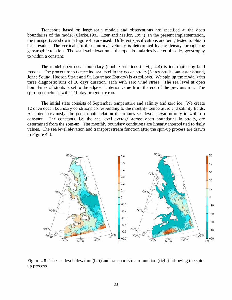
31
Transports based on large-scale models and observations are specified at the open boundaries of the model (Clarke1983 Ezer and Mellor 1994) In the present implementation the transports as shown in Figure 45 are used Different specifications are being tested to obtain best results The vertical profile of normal velocity is determined by the density through the geostrophic relation The sea level elevation at the open boundaries is determined by geostrophy to within a constant
The model open ocean boundary (double red lines in Fig 44) is interrupted by land masses The procedure to determine sea level in the ocean straits (Nares Strait Lancaster Sound Jones Sound Hudson Strait and St Lawrence Estuary) is as follows We spin up the model with three diagnostic runs of 10 days duration each with zero wind stress The sea level at open boundaries of straits is set to the adjacent interior value from the end of the previous run The spin-up concludes with a 10-day prognostic run
The initial state consists of September temperature and salinity and zero ice We create
12 open ocean boundary conditions corresponding to the monthly temperature and salinity fields As noted previously the geostrophic relation determines sea level elevation only to within a constant The constants ie the sea level average across open boundaries in straits are determined from the spin-up The monthly boundary conditions are linearly interpolated to daily values The sea level elevation and transport stream function after the spin-up process are drawn in Figure 48
Figure 48 The sea level elevation (left) and transport stream function (right) following the spin-up process
32
44 Ice categories
The ice model is implemented with 10 ice thickness categories with boundaries at 005 018 038 066 106 158 224 304 398 and 504 m The corresponding central thicknesses c
ih are 0 012 028 052 086 132 191 254 351 and 451 m 5 Model Physics of WaveWatch III (WW3)
The WAVEWATCH III (hereafter WW3) wave model (version 222) is used in the BIO forecasting system to forecast wave height and direction This is a WAM-type ocean surface wave model developed at NOAANCEP (Tolman and Chalikov1996 Tolman 2002) It has been successfully applied in global and regional scale studies in many areas including the North Atlantic and has proven to be an effective tool to study wave spectral evaluation air-sea interactions and nonlinear wave-wave interactions WW3 is a discrete spectra and phase-averaged model (Battjes 1994)
For regional and global applications the directional wave spectrum is resolved at each model grid point in terms of wavenumber-direction bands and the evolution of the wave field is found by numerically solving the spectral wave action balance equation which is usually written as
σθ
θλ
λθφ
φφSNNk
kNN
tN
g =partpart
+partpart
+partpart
+partpart
+partpart ampampampamp cos
cos1 (5-1)
where λ is longitude φ is latitude θ is wave propagation direction k is wave number t is time σ is the intrinsic angular frequency WW3 evaluates the balance equation for the wave action spectrum )( txkN θ which is usually expressed in spherical coordinates (Komen et al 1994)
The derivatives in (5-1) are the propagation velocities in physical and spectral domains
RUcg φθ
φ+
=cosamp
φθ
λ λ
cossinR
Ucg +=amp
Rcg
g
θφθθ
costanminus= ampamp R is the radius of the earth and
φU and λU are current components in φ and λ directions The left side of equation (1) represents the local rate of change of wave action density propagation in physical space action density shifting in frequency and direction due to the spatial and temporal variation in depth and current The net source term S consists of wind input( inS )white-capping dissipation( dsS ) nonlinear wave-wave interactions( nlS ) and bottom friction( botS ) WW3 uses an explicit scheme to solve the action balance equation (1) for N
Two combinations of the source terms inS and dsS are available in WW3 The default set up of WW3 corresponds to the wave-boundary layer formulation for inS and dsS due to Tolman and Chalikov (1996) Tolman (2002) notes that application of this formulation has entailed a
33
correction in fetch-limited wave heights that results from atmospheric stratification which necessitates a re-tuning of the model by defining an lsquoeffectiversquo wind as well as an additional correction for the impact of stability on wave growth An alternate combination corresponds to WAM cycle 3 physics (hereafter denoted WAMC3 physics) in which inS and dsS are based on WAMDI (1988) Snyder et al (1981) and Komen et al (1994) Quadruplet nonlinear interactions nlS are simulated by DIA and bottom dissipation bfS by the JONSWAP parameterization of Hasselmann et al (1973) Padilla-Hernatildendez et al [2007] compared the WW3 model against WAM and SWAN models for two North Atlantic storms and found that WW3 provided the high quality statistical comparisons to deep water observations 6 The Bedford Institute Ocean Forecasting System (BIOFS) BIOFS is a real-time short-term (2-day) forecasting system for eastern Canadian waters The forecast period is constrained by input data from Environment Canada If meteorological data from long range weather forecasts are available the ocean forecasts can be extended to a longer period It consists of two sub-systems one for CECOM (Section 63) and one for WW3 (Section 64) Graphic display of the forecasts can be viewed at the following public website maintained by DFO httpwwwmardfo-mpogccascienceoceanicemodelice_ocean_forecasthtml The parameters displayed on the website are surface trajectories water level time series at selected locations ice concentration and thickness wave height and direction (Northwest Atlantic and Atlantic Maritimes) sea surface elevation (non-tidal) maps temperature at surface and 50 m They are given at hourly (water level time series) 6-hourly (wave) or 12-hourly (all others) intervals 61 Input Data Meteorological Data Meteorological forcing is taken from the Canadian Meteorological Centre (CMC) Global Environmental Multiscale (GEM) model (Mailhot et al 2006) which provides 48 hour forecasts twice daily at 0000 and 1200 UTC with fields output at 3 hour intervals The GEM model is an operational atmospheric model that is part of the Canadian Regional Forecast System (RFS) developed by Environment Canada The model uses a variable resolution grid over the entire globe with a mesoscale 15 km horizontal resolution window over Northern America Fields used in the forecasting system are 10m winds 2m air and dew point temperatures total cloud coverage and total accumulated precipitation All meteorological parameters are linearly interpolated to the ocean and wave model grids Except for the10 m winds the parameter values change every 3 hours For CECOM the 10m wind field is interpolated in time to the model time step of 75 minutes to avoid temporal discontinuities in the dynamical forcing Total accumulated
34
precipitation is converted to a precipitation rate For WW3 the wind fields are interpolated to the propagation time step of the respective wave model (see Section 64 for details) Sea-Ice Data Ice concentration data are used for data assimilation (Section 62) in the ice model and to define the wave domain in WW3 In WW3 a grid point is considered open ocean if the ice concentration is equal or less than 05 Otherwise it is considered land Digital sea ice charts which include ice concentration data are provided by Canadian Ice Services(CIS) Canadian waters are covered by five digital ice charts (Figure 61) Data from Eastern Arctic Hudson Bay and East Coast are used in the forecasting system CIS produces daily charts for the Gulf of StLawrence and the Labrador and Newfoundland coasts south of 58N Regional charts for Hudson Bay Baffin Bay and the Labrador coast north of 58N are produced fortnightly Typically the regional charts are released several days after the date for which they are valid Since these charts represent more of a two week average condition than an instantaneous one BIOFS uses a regional charts release date as its valid date
Figure 61 Coverage of CISrsquos digital ice charts (courtesy of CIS) The digital charts use the ldquoegg coderdquo (Environment Canada 2005) to indicate the sea ice partial concentration for each stage of development on a regularly spaced grid Each ldquoeggrdquo indicates up to three different ice types (ignoring trace amounts) each of which is assigned a stage and concentration The stage of development may be interpreted as an approximate
35
measure of the ice thickness The conversion of stage to ice model thickness category is illustrated in Table 61 There are also four special cases listed in Table 62 Table 61 Conversion from ice stage to ice model category
Ice stage of development Description
Ice model
categoryIce thickness
boundaries (m)
OW BW IF Open Water bergy water ice-free 1 -005 lt h le 005
1 New 2 005 lt h le 018
2 Nilas 2 005 lt h le 018
3 Young Unknown 3 018 lt h le 038
4 Young Grey 2 005 lt h le 018
5 Young Grey-White 3 018 lt h le 038
6 First Year Unknown 4 038 lt h le 066
7 First Year Thin 5 066 lt h le 106
8 First Year Thin First Stage 5 066 lt h le 106
9 First Year Thin Second Stage 5 066 lt h le 106
1 First Year Medium 6 106 lt h le 158
4 First Year Thick 7 158 lt h le 224
7 Old 8 224 lt h le 304
8 Old Second Year 9 304 lt h le 398
9 Old Multi-Year 9 304 lt h le 398
L Ice of Land Origin 9 304 lt h le 398
B Brash 3 018 lt h le 038
Each stage of development is first converted to a category The partial concentrations
and categories including flags (Table 62) are then nearest-neighbour interpolated to the model grid Grid points with land fast ice will be filled with neighbouring concentrations and categories Including flags in the interpolation preserves grid points which should not be filled by interpolation All the charts available for a forecast date are then combined Where charts overlap the concentrations of each category are averaged Flagged points are ignored in the averaging
36
Table 62 Interpolation of ice data
Ice stage of
development Description Action
POINT NOT COVERED BY
POLYGON Point is outside CIS analysis area Flag
LAND Land point Flag
ICEGLACE Useless CIS category indicating ice presence but not providing concentration or stage
Flag
FASTICE Land fast ice Nearest Neighbour
Tides Tidal constituents of elevation and velocity come from two sources Paturi et al (2008) provides eight constituents (M2 S2 N2 K2 K1 O1 P1 Q1) and covers most of the model domain up to Davis Strait Dunphy et al (2005) provides five tidal constituents (M2 S2 N2 K1 O1) for Baffin Bay Constituents are linearly interpolated to the model grid Where the two sources slightly overlap at Davis Strait matching constituents are averaged 62 Data assimilation in CECOM
Many assimilation schemes have been developed for oceanographic and meteorological applications in the past 20 years Advanced schemes such as 3-d and 4-d variational method and Karmen filter require massive resources and abundant data to yield optimum results In this section we describe three methods to assimilate the annual cycle of the temperature and salinity fields sea surface temperature and ice concentration data into the ocean forecast model Assimilation of the Annual Cycle of the Temperature and Salinity Fields Monthly temperature and salinity climatologies are prescribed at the open boundaries of CECOM Such constraints are not strong enough to prevent the temperature and salinity fields from drifting in multi-year integration To ensure the annual cycles are preserved a nudging term with a constant relaxation time scale tR of 45 days are added to the temperature and salinity equation
37
)(1 TTtt
TCLIM
R
minus+=partpart
)(1 SStt
SCLIM
R
minus+=partpart
where TCLIM and SCLIM are monthly temperature and salinity climatologies linearly interpolated to daily intervals Assimilation of Sea Surface Temperature Data Daily near real-time sea surface temperature (SST) derived mainly from satellite observations are provided by CMC The data are assimilated into the ocean forecast model using a flux correction method The method is based on the theory of optimal interpolation A correction term proportional to the differences between the modeled and observed SST is added to the heat flux equation
We first consider the equation for SST assimilation (see Appendix 4)
( ) [ ])()(
2exp)()( 2
2
22
2
om
ooo
om
mma tTtTtt
tTtT minus⎥⎥⎦
⎤
⎢⎢⎣
⎡ minusminus
++=
τεεε
(61)
where the superscripts and subscripts ldquoardquo ldquomrdquo and ldquoordquo in (61) denote ldquoassimilationrdquo ldquomodelrdquo and ldquoobservationrdquo respectively to is the time of the most recent observation and t is the model time 2
mε and 2oε are the model and data errors respectively τ is the correlation time scale of
SST Since change in SST ΔT is related to change in heat flux ΔQ by
Qhc
tT
p
d Δ=Δρ
where h is the mixed layer depth and td is the time interval of SST data the first terms on each side of (61) can be replaced by the corresponding heat fluxes The equation for SST data assimilation is
( ) [ ])()(2
exp)()( 2
2
om
ooo
d
pma tTtTtt
Ft
hctQtQ minus
⎥⎥⎦
⎤
⎢⎢⎣
⎡ minusminus+=
τρ
(62)
where F = 1 [1+ (εο εm)2] F ranges from 0 to 1 Not all parameters in (62) are well known To implement (62) in the forecast model the parameters are adjusted to yield optimal results
38
Figures 62 and 63 show the impact of data assimilation on model SST from a test run In this run F = 1 td = 1 day τ = 1 day were used and h = 20 m To reduce model noise in the run )( o
m tT in (62) was replaced by the model SST averaged over the previous day (from t0 - 1 day to t0) Significant improvements in the model SST can be achieved by using this assimilation scheme Without data assimilation the difference between the model and data at the Scotian Shelf is of the order of ~ 2o C The difference is reduced to a fraction of a degree with data assimilation Over the model domain the model without data assimilation over predicts SST in the northern Labrador Sea and under predicts SST in the coastal and the North Atlantic Current regions (Figs 63) Data assimilation is able to reduce the errors to less than 1o C
The SST assimilation is applied to ice free waters only In ice covered areas the sea
surface temperature is equal or very close to the freezing temperature
Figure 62 A comparison of SST in a 1o x 1o area centered at the indicated location with and without data assimilation
39
Figure 63 CMC SST (left) and the difference between the model and data with (middle) and without (right) data assimilation Assimilation of sea-ice data An insertion-nudging method is used for ice data assimilation Ice concentration data are inserted to the model gradually and the model concentration is restored to the data value with a prescribed time constant In the equation for the thickness distribution function a term proportional to the difference between the observed and values is introduced
( ) ( ))( ioi
iiice
i ggdiffusionhfg
gt
gminusΓ++Ψ=
partpart
+sdotnabla+part
partu (62)
where goi is the ice chart concentrations and gi is the model concentrations for ice of thickness category i Γ has the following form
⎥⎦
⎤⎢⎣
⎡ minusminus=Γ 2
2
2)(
expw
om
ttγ
γ (63)
where t is the model time to is the time for which the ice chart is valid γm and γw are adjustable parameters The Gaussian function in (63) limits nudging to the times around the ice chart time 1γm is the restoring time scale In the present implementation the values of 1γm and γw are set to 16 hours (5760 seconds) and 3 hours (10800 seconds) respectively At one hour from the ice chart time this scheme gives a concentration change rate of ~05 per hour At times plusmn 2γw from
40
the ice chart time the rate is negligible Where there is no ice chart data the nudging is not applied Figure 64 is a comparison of ice area south of 58o with and without data assimilation for January 2008 Figure 65 shows the ice concentration from CISrsquos East Coast ice chart and the model results with and without data assimilation The data assimilation significantly reduces the model error In particular ice cover in the Gulf of St Lawrence and the location of the eastern ice edge can be simulated more realistically with data assimilation
Figure 64 A comparison of the model ice area south of 58o N with (blue) and without (black) data assimilation The unit is percentage of the model area south of 58o N
41
Figure 65 Ice concentration for January 28 2008 data (left) model results without (middle) and with (right) data assimilation 63 Operational Implementation of CECOM The ice-ocean component of BIOFS is mostly comprised of MATLAB scripts that handle the pre-processing of model input fields the execution of the CECOM FORTRAN executable the post-processing of model results and the management of data files MATLAB was chosen for its platform independence interpolation and graphics functionalities and the abundance of open source tools such as M_Map (Pawlowicz 2006) readgrib (Blanton 2005) snctools (Evans 2007) and T_Tide (Pawlowicz et al 2002) Scheduling and automation is handled by the Linux bash shell but could easily be implemented for other platforms and operating systems Delivery of Meteorological and ice Data
As with any endeavor in real-time forecasting the primary concern is the timely delivery of the data required to force the forecast model To address this concern a separate subsystem written in bash shell scripts automates the retrieval of crucial meteorological forecast data transmitted from CMC to BIO server Emerald2 twice a day The subsystem polls the site for data and performs file checks after retrieval to verify file integrity There is usually a 5-6 hour delay between the CMC regional forecast and the appearance of the forecast data on their ftp site If the system fails to retrieve the data it retries for a predefined number of times The digital ice charts valid for 1800 UTC are delivered daily to an ftp server at BIO Starfish at ~2200 UTC The CIS delivery system itself checks for file integrity after delivery
42
Forecast Schedule CECOM is run three times daily within BIOFS producing 48 hour forecasts for 0000 and 1200 UTC (Table 63 Fig 66) Due to delays in receiving the meteorological data the CMC 1200 UTC data are received at ~1700-1800 UTC and the forecast completes at ~1800-1900 UTC A 1200 UTC data assimilation run using 1800 UTC sea ice concentration data and 1200 UTC sea surface temperature data (the same SST are received in the CMC 0000 UTC forecast data) is made the following morning at ~0300 UTC to assimilate the most recent ice chart and sea surface temperature data The 0000 UTC forecast is run four hours following the data assimilation run at ~0700 UTC Table 63 Ocean forecast schedule Both the local time ldquoATrdquo (Atlantic Time) and UTC are indicated
Day 1 Day 2
1 ndash 2 pm AT 2 ndash 3 pm AT 6 pm AT 11 pm AT 1 ndash 2 am AT 3 am AT
1700-1800 UTC 1800-1900 UTC 2200 UTC 0300 UTC 0500-0600 UTC 0700 UTC
CMC 1200 UTC forecast data
received
1200 UTC 48-hour forecast
CIS charts received
1200 UTC 48-hour ice
and SST assimilation
CMC 0000 UTC forecast data received
0000 UTC 48-hour forecast
43
Figure 66 Flow chart of the forecasting operations in a 24-hour period Forecast Methodology Each forecast is initialized with the most recent output of a previous forecast The ocean lateral boundary conditions are linearly interpolated to daily values from the monthly means to prevent discontinuity The boundary conditions also provide a constraint for temperature and salinity near the boundaries In the interior nudging and statistical interpolation are used to prevent long-term drifts and to assimilate sea surface temperature data into the model (see Section 62)
CMC 1200UTC data
CIS 1800UTC data
CMC 0000UTC data
12 UTC
forecast run
Data assim
ilation run
00 UTC
forecast run
1200 UTC forecasts
0000 UTC forecasts
Day 1 Day 2 Day 3
Ice concentration data
Sea surface temperature data
Add tide and Stokes drift
Add tide and Stokes drift
44
After the model run T_Tide (RPawlowicz et al 2002) calculates the tidal current and
elevation for the forecast period The tidal components are then linearly added to the forecast components For surface currents wave induced Stokes drifts are added to the model surface current to obtain the total surface current (Tang et al 2007) The Stokes drift us is obtained from the 2-dimensional wave spectrum E (f θ) of WW3 by integrations over frequency and direction
( )intint= θθπ dfdfEef kz
s 4 2ku (64)
where f is wave frequency θ is wave direction k is wave number and k is the magnitude of k
There are two options for the Strokes drift in the forecasting system us can be computed directly from (64) at every model grid point A simpler method is to parameterize us by surface winds us = a W + b W2 (65)
β = turning angle (positive for clockwise) relative to wind direction (66) where us and β are the magnitude and direction of us respectively and W is 10 m wind speed The parameters a b and β are determined from least-squared fits of the Strokes velocities computed from (64) for October-December 2007 In most applications (eg surface drifter floating object) vertically averaged surface currents are required The Stokes velocities in (65) and (66) are replaced vertically averaged Stokes velocities The results of the least-squared fits are given in Table 64 for different depths of averaging Table 64 Parameters values of the Stokes drift for different depths of averaging Depth (m) 1000a 1000b β (deg)
1 2525 0641 380 2 1656 0533 400 3 1176 0459 410 4 0889 0405 430 5 0699 0363 440
Drift tracks are calculated from the total surface current field Each track starts at a model grid point and is advected by the surface current Horizontal linear interpolation is used to calculate the surface current field between grid points Distances are calculated using the plane sailing method which ignores the earths curvature
45
For ice forecasts all available 1800 UTC ice charts from the previous day are processed and assimilated into the model to correct the model ice field as described in Section 62 For ocean forecasts 1200 UTC SST data from the previous day are assimilated into the model (Figure 66) 64 Operational Implementation of WW3
The wave models are implemented on a system of three nested grids (Figures 67 68 69 and Table 65) The spatial resolution increases from 10o in the coarse grid to 05o in the intermediate grid to 01667o (10rsquo) in the fine resolution grid This system of grids ensures that energy from distant storms is not lost in simulating storms making landfall in coastal areas of North America The grid dimensions and resolutions are given in Table 65 Etopo2 bathymetry is used from the United States National Geophysical Data Center at 2 minutes resolution WW3 is used for the coarse intermediate and fine resolution simulations Following the Courant-Friedrichs-Leacutevy (CFL) stability criterion the propagation time steps for WW3 are 20 and 10 minutes for the coarse and intermediate grids respectively and 4 minute propagation steps for the fine-resolution grid In Table 65 WW3 has 4 time steps Δtg is the global time step by which the entire wave model solution is propagated forward in time Δtρ1 is the maximum spatial (xy) propagation time step for the lowest frequency which is required to satisfy the CFL criterion Δtis is the maximum intra-spectral (k θ) propagation time step which is also required to satisfy the CFL criterion and Δtst is the minimum time step for the integration of the source terms which is dynamically adjusted for each grid and for Δtg
WW3 interpolates the wind fields to the propagation time step of the respective wave model For fast moving storms WW3 has a built-in scheme to reduce the source term integration time step when the situation is changing rapidly Moreover in WW3 the source term integration time step can be set by the user Thus we set the minimum source term time step to 5 minutes in the coarse-resolution grid to adequately simulate the storms considered here For the intermediate and fine grids source term time steps were both set to 25 (see Table 65) Details regarding the spectral range and resolution of the WW3 model are given in Table 66 in terms of the lowest and highest frequencies ( lowf and highf ) number of points ( n ) frequency resolution ( fΔ ) and angular resolutions ( θΔ ) The 48-hour WW3 wave forecasts run twice daily (0000 UTC and 1200UTC) WW3 simulates waves outside nearshore areas where shallow water wave processes are not important The model includes standard physics for wave propagation growth by wind nonlinear interactions dissipation due to whitecapping and dissipation due to bottom friction In coastal estuary and nearshore areas where water depth is shallow fine-resolution computational domains are sometimes needed for dedicated studies nested within coarserndashresolution basin-scale domains in order to resolve complex topography coastline features and shallow water wave physics In these special cases an option is that the shallow water SWAN wave model (version 4031) can be applied for a fourth domain nested within the third domain (Ris et al 1994 Booij et al 1996 Booij et al 1999 Holthuijsen et al 2003 Booij 2004) in these specific areas The physics of SWAN are different from that of WW3 especially for shallow water waves
46
SWAN can simulate shoaling refraction bottom friction and depth-induced wave breaking besides the processes for whitecapping wind input and nonlinear wave-wave interactions that are present in WW3 SWAN is formulated in terms of an action balance equation Xu et al (2007) describe the implementation of WW3 and nested grids for the North Atlantic and SWAN for Lunenburg Bay for studies related to the waves generated by hurricane Juan (September 28-29 2003)
Figure 67 Model domain of WW3 - Atlantic Ocean and sample model output (0600 UTC November 4 2007) The colors indicate significant wave height The arrows indicate wave period and direction
47
Figure 68 Model domain of WW3 ndash Northwestern North Atlantic Ocean and sample model output (0600 UTC November 4 2007) The colors indicate significant wave height The arrows indicate wave period and direction
48
Figure 69 Model domain of WW3 ndash Atlantic maritimes and sample model output (0600 UTC November 4 2007) The colors indicate significant wave height The arrows indicate wave period and direction
49
Table 65 Geographical location of the grids used in this study λ θΔ are the resolutions in longitude λ and latitudeφ and Nλ and Nφ are the number of points in λ and φ Finally tΔ is the propagation time step and tΔ ST is the required time step for source term integration for the three models as required to satisfy the CFL criterion GRIDS Longitude Latitude λ θΔ Nλ Nφ Δtg tΔ ST
Coarse 40oE ndash 82oW 75oSndash 77oN 1o 123 153 20 min 50 min
Intermediate 40oWndash75oW 20oN-75oN 05o 71 111 10 min 2min
Fine 47oWndash71oW 42oN-52oN 10rsquo 145 61 5 min 25 min
Table 66 Spectral domains for all models lowf highf are the default values
Parameters Value
lowf highf [s-1] 00418 06028
nf fΔ 29 11 ftimes
θn θΔ 36 10o
50
References Battjes JA 1994 Shallow water wave modelling Proc Int Symp Waves -Phys Numerical
Modelling University of British Columbia Vancouver I 1-23 Budyko MI 1974 Climate and Life Academic Press New York 508 pp Blanton B 2005 readgrib
httpwwwopnmlunceduOPNML_Matlabread_gribread_gribhtml Blumberg AF and GL Mellor 1987 A description of a three-dimensional coastal ocean
circulation model in Three-Dimensional Coastal Ocean Models Coastal Estuarine Sci 4 edited by NS Heaps pp 1-16 AGU Washington DC
Booij N LH Holthuijsen and RC Ris 1996 The ldquoSWANrdquo Wave Model For Shallow Water
Coastal Engineering 1 668~672
Booij N RC Ris and LH Holthuijsen 1999 A third-generation wave model for coastal regions Part I Model description and validation J Geophys Res 104 C4 7649-7666
Booij N 2004 SWAN Cycle III version 4041 user manual[Available online at httpfluidmechanicstudelftnlswanindexhtm]
Carton JA G Chepurin and X Cao 2000 A simple ocean data assimilation analysis of the
global upper ocean 1950-95 Part I methodology J Phys Oceanogr 30 294-309 Charnock H 1955 Wind stress on a water surface Quarterly Journal of Royal Meteorological
Society 81 pp 639ndash640 Clarke RA 1984 Transport through the Cape Farewell-Flemish Cap section Rapp PV Reun
Cons Int Explor Mer 185 120-130 Dunphy M F Dupont C G Hannah D Greenberg 2005 Validation of a modelling system for
tides in the Canadian Arctic Archipelago Can Tech Rep Hydrogr Ocean Sci 243 vi + 70 pp
Dunlap E BM Detracey and CL Tang 2007 Short-wave radiation and sea ice in Baffin Bay
Atmosphere-Ocean 45 195-210 Environment Canada 2005 ldquoMANICE - Manual of Standard Procedures for Observing and
Reporting Ice Conditionsrdquo httpice-glacesecgcca AppWsvPageDspcfmLang=engamplnid=23ampScndLvl=noampID=172
Evans J 2007 snctools httpmexcdfsourceforgenet
51
Ezer T and GL Mellor 1994 Diagnostic and prognostic calculations of the North Atlantic circulation and sea level using a sigma coordinate ocean model J Geophys Res 99 14159-14171
Flato GM 1994 McPIC Documentation for the multi-category particle-in-cell sea ice model
Can Tech Rep Hydrogr Ocean Sci 158 74 pp Gill AE 1982 Atmosphere-Ocean Dynamics Academic Press New York 662 pp Hasselmann K TP Barnett E Bouws H Carlson DE Cartwright K Enke JI Ewing H
Gienapp DE Hasselmann P Kruseman A Meerbrug P Muumlller DJ Olbers K Richter W Sell and H Walden 1973 Measurements of wind-wave growth and swell decay during the Joint North Sea Wave Project (JONSWAP) Dtsch Hydrogr Z A8(12) 95 pp
Hibler WD 1979 A dynamic thermodynamic sea ice model J Phys Oceanogr 9 815-846 Hibler WD 1980 Modeling a variable thickness sea ice cover Mon Wea Rev 108 1943-
1973 Holthuijsen L H and HN Booij 2003 Phase-decoupled refraction-diffraction for spectral
wave models Coastal Engineering 49 291-305 Jerlov NG 1968 Optical Oceanography 194 pp Elsevier Komen G J LCavaleri M Donelan M Hasselmann S Hasselmann P A E M Janssen
1994 Dynamics and Modeling of Ocean Waves Cambridge University Press 520pp Mailhot J S Beacutelair L Lefaivre B Bilodeau M Desgagneacute C Girard A Glazer A-M Leduc
A Meacutethot A Patoine A Plante A Rahill T Robinson D Talbot A Tremblay P Vaillancourt A Zadra A Qaddouri 2006 The 15-km Version of the Canadian Regional Forecast System Atmos-Ocean 44 133-149 DOI 103137ao440202
Martinsen EA and H Engedahl 1987 Implementation and testing of a lateral boundary
scheme as an open boundary condition in a barotropic ocean model Coastal Eng 11 603-627
Mellor GL and AF Blumberg 1985 Modeling vertical and horizontal diffusivities with the
sigma coordinate system Mon Wea Rev 113 1380-1383 Mellor GL and LH Kantha 1989 An ice-ocean coupled model J Geophys Res 94
10937-10954 Mellor GL and T Ezer 1991 A Gulf Stream model and an altimetry assimilation scheme J
Geophys Res 96 8779-8795
52
Mellor GL S Hakkinen T Ezer and R Patchen 2002 A generalization of a sigma coordinate ocean model and an intercomparison of model vertical grids in Ocean Forecasting Conceptual Basis and Applications edited by N Pinardi and J Woods pp 55-72 Springer Berlin
Mellor GL and AF Blumberg 2004 Wave breaking and ocean surface layer thermal
response J Phys Oceanogr 34 693-698 Padilla-Hernatildendez R W Perrie B Toulany and P C Smith 2007 Intercomparison of third
generation wave models Weather and Forecasting Vol 22 No 6pages 1229-1242 Parkinson C L and W M Washington 1979 A large-scale numerical model of sea ice J
Geophys Res 84 311-337 Paturi S G Han and B deYoung 2008 A 3-D multi-constituent data assimilative tidal model
of the northwest Atlantic Atmosphere-Ocean Submitted Paulson CL and JJ Simpson 1977 Irradiance measurements in the upper ocean J Phys
Oceangr 7 952-956 Pawlowicz R 2006 M_Map httpwwweosubcca~rich Pawlowicz R B Beardsley and S Lentz 2002 Classical tidal harmonic analysis including
error estimates in MATLAB using T_TIDE Computers and Geosciences 28 929-937 httpwwweosubcca~rich
Perrie W Gunther H Rosenthal W and Toulany B 1989 Modelling wind - generated
surface gravity waves using similarity Quart J Roy Met Soc 115 1373-1396 Ris RC Holthuijsen LH and Booij N 1994 A Spectral Model for Waves in the Near shore
Zone Coastal Engineering 1 68~78 Semtner AJ 1976 A model for the thermodynamic growth of sea ice in numerical
investigations of climate J Phys Oceanogr 67 379-389 Shine KP 1984 Parameterization of the shortwave flux over high albedo surfaces as a
function of cloud thickness and surface albedo Q J R Meterol Soc 110 747-764 Sloslashrdal LH EA Martinsen and AF Blumberg 1994 Modeling the response of an idealized
coastal ocean to a traveling storm and to flow over bottom topography J Phys Oceanogr 24 1698-1705
Smith SD 1988 Coefficients for sea surface wind stress heat flux and wind profiles as a
function wind speed and temperature J Geophys Res 93 15467-15472
53
Smith SD and FW Dobson 1984 The heat budget at Ocean Weather Station Bravo Atmos-Ocean 22 1-22
Snyder RL FW Dobson JA Elliot and RB Long 1981 Array measurements of
atmospheric pressure fluctuations above surface gravity waves J Fluid Mech 20 1166-1174
Tang CL 2007 High-resolution monthly temperature and salinity climatologies for the
northwestern North Atlantic Ocean Canadian Data Report of Hydrography and Ocean Sciences No 169 iv + 55 pp
Tang CL Q Gui and I Peterson 1996a Modeling the mean circulation of the Labrador Sea
and the adjacent shelves J Phys Oceangr 26 1989-2010 Tang CL and Q Gui 1996b A dynamical model for wind-driving ice modtion ndash applicaton to
ice drift on the Labrador Shelf J Geophys Res 101 28343-28364 Tang CL CK Ross T Yao B Petrie BM Detracey and E Dunlap 2004 The circulation
water masses and sea ice of Baffin Bay Progress of Oceanography 63 183-228 Tang CL W Perrie AD Jenkins BM Detracey Y Hu B Toulany and PC Smith 2007
Observation and modeling of surface currents on the Grand Banks a study of the wave effects on surface currents J Geophys Res 112 C10025 doi1010292006JC004028
Thorndike AS DA Rothrock GA Maykut and R Colony 1975 The thickness distribution
of sea ice J Geophys Res 80 4501-4513 Tolman H L 2002 User manual and system documentation of WAVEWATCH-III version
222 Technical Note [Available online at httppolarncepnoaagovwaves] Tolman H L and Chalikov DV 1996 Source terms in a third-generation wind-wave model J
Phys Oceanogr 26 2497-2518 WAMDI group 1988 The WAM model ndash a third generation ocean wave prediction model J
Phys Oceanogr 18 1775-1810 Xu F W Perrie B Toulany and P C Smith 2007 Wind-generated waves in Hurricane Juan
Ocean Modelling Vol 16 pages 188ndash205 Yao T CL Tang and IK Peterson 2000 Modeling the seasonal variation of sea ice in the
Labrador Sea with a coupled multi-category ice model and the Princeton Ocean Model J Geophys Res 105 1153-1165
Yao T CL Tang 2003 The formation and maintenance of the North Water Atmosphere-
Ocean 41 187-201
54
Zhang J and WD Hibler 1997 On an efficient numerical method for modeling sea ice dynamics J Geophys Res 102 8691-8702
55
Appendix 1 Turbulence closure
This appendix outlines the calculations of the vertical mixing coefficients from turbulence closure Governing equations for turbulence kinetic energy q22 and turbulence macroscale l are
)(222 2
1
322
22222
qAlB
qz
Kgzv
zuK
zqK
zzqw
yqv
xqu
tq
HHo
M
q
nablasdotnabla+minuspartpart
+⎥⎥⎦
⎤
⎢⎢⎣
⎡⎟⎠⎞
⎜⎝⎛
partpart
+⎟⎠⎞
⎜⎝⎛
partpart
+
⎟⎟⎠
⎞⎜⎜⎝
⎛part
partpartpart
=part
part+
partpart
+part
part+
partpart
ρρ
)(~ 2
1
31
22
1
22222
lqAwBq
zKglE
zv
zuKlE
zlqK
zzlqw
ylqv
xlqu
tlq
HHo
M
q
nablasdotnabla+minuspartpart
+⎥⎥⎦
⎤
⎢⎢⎣
⎡⎟⎠⎞
⎜⎝⎛
partpart
+⎟⎠⎞
⎜⎝⎛
partpart
+
⎟⎟⎠
⎞⎜⎜⎝
⎛part
partpartpart
=part
part+
partpart
+part
part+
partpart
ρρ
where
2
21~ ⎟⎠⎞
⎜⎝⎛+=
LlEw
κ
( ) ( ) 111 minusminusminus ++minus= zHzL η
κ is the von Karman constant and B1 E1 and E2 are empirical constants
The effects of wave breaking are taken into consideration through the surface boundary condition for q2 At the surface the vertical gradient of q2 is proportional to the cube of the water friction velocity (Mellor and Blumberg 2004) A consequence of this boundary condition is that the eddy viscosity is non-zero at the surface (Tang et al 2007) The boundary conditions at the surface are
⎪⎩
⎪⎨⎧
=
=part
partlowast
covered ice
free ice22
321
2
32
uBq
uz
qBCα
02 =lq
where αBC is a prescribed constant and u is the friction velocity
56
020
20
2 )( ρττ yxu +=
The boundary conditions at the ocean bottom are
02
2
321
2
=
=
lq
uBq
where u is derived from the bottom stress
The mixing coefficients KM KH and Kq can be expressed in terms of stability functions SM SH and Sq
)()( qHMqHM SSSlqKKK = The stability functions are derived from the solution of analytic equations (Blumberg and Mellor 1987) involving the vertical shear and vertical density gradient In the presence of ice the mixing coefficient is the average of the values for open ocean and for ice-covered ocean (no wave effects) weighted by ice concentration Appendix 2 Generalised sigma coordinates
Generalised sigma coordinates are derived by transforming coordinates (x y z t) to (x y s t) The vertical coordinate s is defined
)()( tyxtkyxsz η+= (A21) where s is a function of the vertical variable k which ranges from 1 at the surface to kb at the ocean bottom For the purposes of this discussion k is continuous but it is discrete for the computer implementation Since 0 =partpart xz then
0
xk
ks
xs
x partpart
partpart
+partpart
+partpart
=η
or
k
xx
ss
xk
η+
minus=partpart
Also the z derivative of (A21) gives
kszk 1
=partpart
57
For a function )( tzyxφ partial derivatives in the old coordinate system are related to partial derivatives in the new coordinate system as
1
k
tt
k
k
yy
k
xx
ss
ktt
skz
ss
kyy
ss
kxx
ηφφφ
φφ
ηφφφ
ηφφφ
+partpart
minuspartpart
=partpart
partpart
=partpart
+partpart
minuspartpart
=partpart
+partpart
minuspartpart
=partpart
We define a new vertical velocity ω as
( ) ( ) yyxxtt svsusw ηηηω ++++++=
The continuity equation in transformed coordinates (henceforth dropping the asterisks) is
0)()(
=partpart
+part
part+
partpart
+part
partky
vsx
ust
s kkk ω (A22)
The momentum equations in transformed coordinates are
( ) ( ) ( ) ( ) ( )
int int +⎟⎟⎠
⎞⎜⎜⎝
⎛partpart
partpart
+partpart
minuspartpart
+
+minus=minuspart
part+
partpart
+part
part+
partpart
xk
Mk
o
kx
o
k
xxkkkkk
Mku
sK
kdk
xsgsdk
ksgs
sgsfvsku
yuvs
xsu
tus
ρρ
ρρ
ηω 22
(A23)
( ) ( ) ( ) ( ) ( )
int int +⎟⎟⎠
⎞⎜⎜⎝
⎛partpart
partpart
+partpart
minuspartpart
+
+minus=+part
part+
partpart
+part
part+
partpart
yk
Mk
o
ky
o
k
yykkkkk
Mkv
sK
kdk
ysgsdk
ksgs
sgsfuskv
ysv
xuvs
tvs
ρρ
ρρ
ηω 22
(A24)
The heat and salt equations in transformed coordinates are
( ) ( ) ( ) ( )
Tk
Hkkk MkT
sK
kkT
yvTs
xuTs
tTs
+⎟⎟⎠
⎞⎜⎜⎝
⎛partpart
partpart
=part
part+
partpart
+part
part+
partpart ω
58
( ) ( ) ( ) ( )S
k
Hkkk MkS
sK
kkS
yvSs
xuSs
tSs
+⎟⎟⎠
⎞⎜⎜⎝
⎛partpart
partpart
=part
part+
partpart
+part
part+
partpart ω
The horizontal mixing terms become
⎥⎦
⎤⎢⎣
⎡⎟⎟⎠
⎞⎜⎜⎝
⎛partpart
+partpart
partpart
+⎟⎠⎞
⎜⎝⎛
partpart
partpart
=xv
yuAs
yxuAs
xM MkMkx 2
⎥⎦
⎤⎢⎣
⎡⎟⎟⎠
⎞⎜⎜⎝
⎛partpart
+partpart
partpart
+⎟⎟⎠
⎞⎜⎜⎝
⎛partpart
partpart
=xv
yuAs
xyvAs
yM MkMky 2
⎟⎟⎠
⎞⎜⎜⎝
⎛partpart
partpart
+⎟⎠⎞
⎜⎝⎛
partpart
partpart
=yTAs
yxTAs
xM HkMkT
⎟⎟⎠
⎞⎜⎜⎝
⎛partpart
partpart
+⎟⎠⎞
⎜⎝⎛
partpart
partpart
=ySAs
yxSAs
xM HkMkS
These forms are not simply the transformations of (28) This relates to separating vertical mixing from horizontal mixing in a coordinate system in which constant k surfaces are sloping (Mellor and Blumberg 1985 and Mellor et al 2002) Appendix 3 Rotated spherical coordinate system
Coordinates r on a unit sphere are transformed to rprime in a rotated system (42) with the matrix R by
rRRRRrr ξης==prime (A31) where Rξ Rη Rζ are transformation matrices for rotations by the individual angles ξ η and ζ respectively (Figure 42)
The individual rotation matrices are
⎟⎟⎟
⎠
⎞
⎜⎜⎜
⎝
⎛minus=
1000cossin0sincos
ξξξξ
ξR ⎟⎟⎟
⎠
⎞
⎜⎜⎜
⎝
⎛ minus=
ηη
ηη
η
cos0sin010
sin0cosR
⎟⎟⎟
⎠
⎞
⎜⎜⎜
⎝
⎛minus=
1000cossin0sincos
ςςςς
ςR (A32)
giving the matrix R as
59
⎟⎟⎟
⎠
⎞
⎜⎜⎜
⎝
⎛+minusminusminus
minus+minus
ηξηξηηςξςξηςξςξηςηςξςξηςξςξης
cossinsincossinsinsincoscossincossinsincoscoscossinsincoscossinsincoscossinsincoscoscos
(A33)
As well as transforming coordinates it is also necessary to transform components of
vectors tangent to the sphere Define α(φθ) as the angle between parallels of latitude (Figure A31) The angle between a vector and the local parallel in the rotated system is the corresponding angle in the original system minus α Denoting longitude and co-latitude in the rotated coordinate system as ( )θφ primeprime then
θφφφθα
sintanprimepartpart
primepartpartminus= (A34)
From (41) (φ θ) are related to (x y z) by tan φ = yx cosθ = z (A35)
The partial derivatives in (A34) may be written as
( ) 212
1
1cosz
zzminus
primepartpartminus=
primepartpart
=primepart
part minus φφφ
θ (A36)
and
( ) ⎟⎟⎠
⎞⎜⎜⎝
⎛primepart
partminus
primepartpart
+=
primepartpart
=primepart
part minus
φφφφφ xyyx
yxxy 22
1 1tan (A37)
Eqs (A36) and (A37) involve derivatives φprimepartpartr From (A31)
⎟⎟⎟
⎠
⎞
⎜⎜⎜
⎝
⎛
primeprimeprimeprimeprime
=⎟⎟⎟
⎠
⎞
⎜⎜⎜
⎝
⎛
primeprimeprime
=⎟⎟⎟
⎠
⎞
⎜⎜⎜
⎝
⎛minusminus
θφθφθ
cossinsincossin
11 RRzyx
zyx
(A38)
The partial derivatives in (A36) and (A37) are then
⎟⎟⎟
⎠
⎞
⎜⎜⎜
⎝
⎛primeprimeprimeprimeminus
=⎟⎟⎟
⎠
⎞
⎜⎜⎜
⎝
⎛
primepartpart
primepartpart
primepartpartminus
0cossinsinsin
1 φθφθ
φφφ
Rzyx
(A39)
60
We obtain α by substituting (A39) into (A36) and (A37) and then substituting (A36) and (A37) into (A34)
Figure A31 The angle α between a parallel of latitude in the rotated coordinate system and a parallel of latitude in the original system enables the transformation of components of a vector Appendix 4 Two-dimensional statistical interpolation Consider a variable Ti at a model time and grid point denoted by the subscript i The model value m
iT is corrected by past or present observations to yield an assimilated value aiT
according to
sum=
minus+=N
moi
mi
ai TTPTT
1)(
αααα (A4-1)
where oTα is the observation and mTα is the model value at the time and location of the observation denoted by the subscript ldquoαrdquo N is the number of observations to be included in the assimilation Piα are weights obtained by minimizing the difference between the model prediction and the observation which are solutions of the following algebraic equations (Mellor and Ezer 1991)
sum=
==+N
ii NMDMP1
21)(α
βαβαβα β (A4-2)
61
where Mαβ and Dαβ are the error matrices for model and observation respectively
oomm TTDTTM βααββααβ ΔsdotΔ=ΔsdotΔ= (A4-3)
mTαΔ and oTαΔ are the model and observation errors respectively The error matrices can be parameterized by a Gaussian and a delta function (Mellor and Ezer 1991 Carton et al 2000)
⎥⎥⎦
⎤
⎢⎢⎣
⎡ minusminus
minusminus
minusminus= 2
2
2
2
2
22
2)(
2)(
2)(
expxyx
m
ttL
yyLxx
Mτ
ε βαβαβααβ (A4-4)
αβαβ δε 2
oD = (A4-5) where Lx Ly and τ are the correlation scales of the model errors If the horizontal correlation scale is much larger than the grid spacing of the model the spatial part of (A4-4) can be neglected and (A4-1) is reduced to
)(2
)(exp 112
21
22
2moi
om
mmi
ai TT
ttTT minus⎥
⎦
⎤⎢⎣
⎡ minusminus
++=
τεεε
(A4-6)
where the subscript ldquo1rdquo denotes the time of the most recent observation ( itt le1 )
- Forecastsystem_18Nov08_Part_1
- Forecastsystem_10Dec08_Part_2
-
32
44 Ice categories
The ice model is implemented with 10 ice thickness categories with boundaries at 005 018 038 066 106 158 224 304 398 and 504 m The corresponding central thicknesses c
ih are 0 012 028 052 086 132 191 254 351 and 451 m 5 Model Physics of WaveWatch III (WW3)
The WAVEWATCH III (hereafter WW3) wave model (version 222) is used in the BIO forecasting system to forecast wave height and direction This is a WAM-type ocean surface wave model developed at NOAANCEP (Tolman and Chalikov1996 Tolman 2002) It has been successfully applied in global and regional scale studies in many areas including the North Atlantic and has proven to be an effective tool to study wave spectral evaluation air-sea interactions and nonlinear wave-wave interactions WW3 is a discrete spectra and phase-averaged model (Battjes 1994)
For regional and global applications the directional wave spectrum is resolved at each model grid point in terms of wavenumber-direction bands and the evolution of the wave field is found by numerically solving the spectral wave action balance equation which is usually written as
σθ
θλ
λθφ
φφSNNk
kNN
tN
g =partpart
+partpart
+partpart
+partpart
+partpart ampampampamp cos
cos1 (5-1)
where λ is longitude φ is latitude θ is wave propagation direction k is wave number t is time σ is the intrinsic angular frequency WW3 evaluates the balance equation for the wave action spectrum )( txkN θ which is usually expressed in spherical coordinates (Komen et al 1994)
The derivatives in (5-1) are the propagation velocities in physical and spectral domains
RUcg φθ
φ+
=cosamp
φθ
λ λ
cossinR
Ucg +=amp
Rcg
g
θφθθ
costanminus= ampamp R is the radius of the earth and
φU and λU are current components in φ and λ directions The left side of equation (1) represents the local rate of change of wave action density propagation in physical space action density shifting in frequency and direction due to the spatial and temporal variation in depth and current The net source term S consists of wind input( inS )white-capping dissipation( dsS ) nonlinear wave-wave interactions( nlS ) and bottom friction( botS ) WW3 uses an explicit scheme to solve the action balance equation (1) for N
Two combinations of the source terms inS and dsS are available in WW3 The default set up of WW3 corresponds to the wave-boundary layer formulation for inS and dsS due to Tolman and Chalikov (1996) Tolman (2002) notes that application of this formulation has entailed a
33
correction in fetch-limited wave heights that results from atmospheric stratification which necessitates a re-tuning of the model by defining an lsquoeffectiversquo wind as well as an additional correction for the impact of stability on wave growth An alternate combination corresponds to WAM cycle 3 physics (hereafter denoted WAMC3 physics) in which inS and dsS are based on WAMDI (1988) Snyder et al (1981) and Komen et al (1994) Quadruplet nonlinear interactions nlS are simulated by DIA and bottom dissipation bfS by the JONSWAP parameterization of Hasselmann et al (1973) Padilla-Hernatildendez et al [2007] compared the WW3 model against WAM and SWAN models for two North Atlantic storms and found that WW3 provided the high quality statistical comparisons to deep water observations 6 The Bedford Institute Ocean Forecasting System (BIOFS) BIOFS is a real-time short-term (2-day) forecasting system for eastern Canadian waters The forecast period is constrained by input data from Environment Canada If meteorological data from long range weather forecasts are available the ocean forecasts can be extended to a longer period It consists of two sub-systems one for CECOM (Section 63) and one for WW3 (Section 64) Graphic display of the forecasts can be viewed at the following public website maintained by DFO httpwwwmardfo-mpogccascienceoceanicemodelice_ocean_forecasthtml The parameters displayed on the website are surface trajectories water level time series at selected locations ice concentration and thickness wave height and direction (Northwest Atlantic and Atlantic Maritimes) sea surface elevation (non-tidal) maps temperature at surface and 50 m They are given at hourly (water level time series) 6-hourly (wave) or 12-hourly (all others) intervals 61 Input Data Meteorological Data Meteorological forcing is taken from the Canadian Meteorological Centre (CMC) Global Environmental Multiscale (GEM) model (Mailhot et al 2006) which provides 48 hour forecasts twice daily at 0000 and 1200 UTC with fields output at 3 hour intervals The GEM model is an operational atmospheric model that is part of the Canadian Regional Forecast System (RFS) developed by Environment Canada The model uses a variable resolution grid over the entire globe with a mesoscale 15 km horizontal resolution window over Northern America Fields used in the forecasting system are 10m winds 2m air and dew point temperatures total cloud coverage and total accumulated precipitation All meteorological parameters are linearly interpolated to the ocean and wave model grids Except for the10 m winds the parameter values change every 3 hours For CECOM the 10m wind field is interpolated in time to the model time step of 75 minutes to avoid temporal discontinuities in the dynamical forcing Total accumulated
34
precipitation is converted to a precipitation rate For WW3 the wind fields are interpolated to the propagation time step of the respective wave model (see Section 64 for details) Sea-Ice Data Ice concentration data are used for data assimilation (Section 62) in the ice model and to define the wave domain in WW3 In WW3 a grid point is considered open ocean if the ice concentration is equal or less than 05 Otherwise it is considered land Digital sea ice charts which include ice concentration data are provided by Canadian Ice Services(CIS) Canadian waters are covered by five digital ice charts (Figure 61) Data from Eastern Arctic Hudson Bay and East Coast are used in the forecasting system CIS produces daily charts for the Gulf of StLawrence and the Labrador and Newfoundland coasts south of 58N Regional charts for Hudson Bay Baffin Bay and the Labrador coast north of 58N are produced fortnightly Typically the regional charts are released several days after the date for which they are valid Since these charts represent more of a two week average condition than an instantaneous one BIOFS uses a regional charts release date as its valid date
Figure 61 Coverage of CISrsquos digital ice charts (courtesy of CIS) The digital charts use the ldquoegg coderdquo (Environment Canada 2005) to indicate the sea ice partial concentration for each stage of development on a regularly spaced grid Each ldquoeggrdquo indicates up to three different ice types (ignoring trace amounts) each of which is assigned a stage and concentration The stage of development may be interpreted as an approximate
35
measure of the ice thickness The conversion of stage to ice model thickness category is illustrated in Table 61 There are also four special cases listed in Table 62 Table 61 Conversion from ice stage to ice model category
Ice stage of development Description
Ice model
categoryIce thickness
boundaries (m)
OW BW IF Open Water bergy water ice-free 1 -005 lt h le 005
1 New 2 005 lt h le 018
2 Nilas 2 005 lt h le 018
3 Young Unknown 3 018 lt h le 038
4 Young Grey 2 005 lt h le 018
5 Young Grey-White 3 018 lt h le 038
6 First Year Unknown 4 038 lt h le 066
7 First Year Thin 5 066 lt h le 106
8 First Year Thin First Stage 5 066 lt h le 106
9 First Year Thin Second Stage 5 066 lt h le 106
1 First Year Medium 6 106 lt h le 158
4 First Year Thick 7 158 lt h le 224
7 Old 8 224 lt h le 304
8 Old Second Year 9 304 lt h le 398
9 Old Multi-Year 9 304 lt h le 398
L Ice of Land Origin 9 304 lt h le 398
B Brash 3 018 lt h le 038
Each stage of development is first converted to a category The partial concentrations
and categories including flags (Table 62) are then nearest-neighbour interpolated to the model grid Grid points with land fast ice will be filled with neighbouring concentrations and categories Including flags in the interpolation preserves grid points which should not be filled by interpolation All the charts available for a forecast date are then combined Where charts overlap the concentrations of each category are averaged Flagged points are ignored in the averaging
36
Table 62 Interpolation of ice data
Ice stage of
development Description Action
POINT NOT COVERED BY
POLYGON Point is outside CIS analysis area Flag
LAND Land point Flag
ICEGLACE Useless CIS category indicating ice presence but not providing concentration or stage
Flag
FASTICE Land fast ice Nearest Neighbour
Tides Tidal constituents of elevation and velocity come from two sources Paturi et al (2008) provides eight constituents (M2 S2 N2 K2 K1 O1 P1 Q1) and covers most of the model domain up to Davis Strait Dunphy et al (2005) provides five tidal constituents (M2 S2 N2 K1 O1) for Baffin Bay Constituents are linearly interpolated to the model grid Where the two sources slightly overlap at Davis Strait matching constituents are averaged 62 Data assimilation in CECOM
Many assimilation schemes have been developed for oceanographic and meteorological applications in the past 20 years Advanced schemes such as 3-d and 4-d variational method and Karmen filter require massive resources and abundant data to yield optimum results In this section we describe three methods to assimilate the annual cycle of the temperature and salinity fields sea surface temperature and ice concentration data into the ocean forecast model Assimilation of the Annual Cycle of the Temperature and Salinity Fields Monthly temperature and salinity climatologies are prescribed at the open boundaries of CECOM Such constraints are not strong enough to prevent the temperature and salinity fields from drifting in multi-year integration To ensure the annual cycles are preserved a nudging term with a constant relaxation time scale tR of 45 days are added to the temperature and salinity equation
37
)(1 TTtt
TCLIM
R
minus+=partpart
)(1 SStt
SCLIM
R
minus+=partpart
where TCLIM and SCLIM are monthly temperature and salinity climatologies linearly interpolated to daily intervals Assimilation of Sea Surface Temperature Data Daily near real-time sea surface temperature (SST) derived mainly from satellite observations are provided by CMC The data are assimilated into the ocean forecast model using a flux correction method The method is based on the theory of optimal interpolation A correction term proportional to the differences between the modeled and observed SST is added to the heat flux equation
We first consider the equation for SST assimilation (see Appendix 4)
( ) [ ])()(
2exp)()( 2
2
22
2
om
ooo
om
mma tTtTtt
tTtT minus⎥⎥⎦
⎤
⎢⎢⎣
⎡ minusminus
++=
τεεε
(61)
where the superscripts and subscripts ldquoardquo ldquomrdquo and ldquoordquo in (61) denote ldquoassimilationrdquo ldquomodelrdquo and ldquoobservationrdquo respectively to is the time of the most recent observation and t is the model time 2
mε and 2oε are the model and data errors respectively τ is the correlation time scale of
SST Since change in SST ΔT is related to change in heat flux ΔQ by
Qhc
tT
p
d Δ=Δρ
where h is the mixed layer depth and td is the time interval of SST data the first terms on each side of (61) can be replaced by the corresponding heat fluxes The equation for SST data assimilation is
( ) [ ])()(2
exp)()( 2
2
om
ooo
d
pma tTtTtt
Ft
hctQtQ minus
⎥⎥⎦
⎤
⎢⎢⎣
⎡ minusminus+=
τρ
(62)
where F = 1 [1+ (εο εm)2] F ranges from 0 to 1 Not all parameters in (62) are well known To implement (62) in the forecast model the parameters are adjusted to yield optimal results
38
Figures 62 and 63 show the impact of data assimilation on model SST from a test run In this run F = 1 td = 1 day τ = 1 day were used and h = 20 m To reduce model noise in the run )( o
m tT in (62) was replaced by the model SST averaged over the previous day (from t0 - 1 day to t0) Significant improvements in the model SST can be achieved by using this assimilation scheme Without data assimilation the difference between the model and data at the Scotian Shelf is of the order of ~ 2o C The difference is reduced to a fraction of a degree with data assimilation Over the model domain the model without data assimilation over predicts SST in the northern Labrador Sea and under predicts SST in the coastal and the North Atlantic Current regions (Figs 63) Data assimilation is able to reduce the errors to less than 1o C
The SST assimilation is applied to ice free waters only In ice covered areas the sea
surface temperature is equal or very close to the freezing temperature
Figure 62 A comparison of SST in a 1o x 1o area centered at the indicated location with and without data assimilation
39
Figure 63 CMC SST (left) and the difference between the model and data with (middle) and without (right) data assimilation Assimilation of sea-ice data An insertion-nudging method is used for ice data assimilation Ice concentration data are inserted to the model gradually and the model concentration is restored to the data value with a prescribed time constant In the equation for the thickness distribution function a term proportional to the difference between the observed and values is introduced
( ) ( ))( ioi
iiice
i ggdiffusionhfg
gt
gminusΓ++Ψ=
partpart
+sdotnabla+part
partu (62)
where goi is the ice chart concentrations and gi is the model concentrations for ice of thickness category i Γ has the following form
⎥⎦
⎤⎢⎣
⎡ minusminus=Γ 2
2
2)(
expw
om
ttγ
γ (63)
where t is the model time to is the time for which the ice chart is valid γm and γw are adjustable parameters The Gaussian function in (63) limits nudging to the times around the ice chart time 1γm is the restoring time scale In the present implementation the values of 1γm and γw are set to 16 hours (5760 seconds) and 3 hours (10800 seconds) respectively At one hour from the ice chart time this scheme gives a concentration change rate of ~05 per hour At times plusmn 2γw from
40
the ice chart time the rate is negligible Where there is no ice chart data the nudging is not applied Figure 64 is a comparison of ice area south of 58o with and without data assimilation for January 2008 Figure 65 shows the ice concentration from CISrsquos East Coast ice chart and the model results with and without data assimilation The data assimilation significantly reduces the model error In particular ice cover in the Gulf of St Lawrence and the location of the eastern ice edge can be simulated more realistically with data assimilation
Figure 64 A comparison of the model ice area south of 58o N with (blue) and without (black) data assimilation The unit is percentage of the model area south of 58o N
41
Figure 65 Ice concentration for January 28 2008 data (left) model results without (middle) and with (right) data assimilation 63 Operational Implementation of CECOM The ice-ocean component of BIOFS is mostly comprised of MATLAB scripts that handle the pre-processing of model input fields the execution of the CECOM FORTRAN executable the post-processing of model results and the management of data files MATLAB was chosen for its platform independence interpolation and graphics functionalities and the abundance of open source tools such as M_Map (Pawlowicz 2006) readgrib (Blanton 2005) snctools (Evans 2007) and T_Tide (Pawlowicz et al 2002) Scheduling and automation is handled by the Linux bash shell but could easily be implemented for other platforms and operating systems Delivery of Meteorological and ice Data
As with any endeavor in real-time forecasting the primary concern is the timely delivery of the data required to force the forecast model To address this concern a separate subsystem written in bash shell scripts automates the retrieval of crucial meteorological forecast data transmitted from CMC to BIO server Emerald2 twice a day The subsystem polls the site for data and performs file checks after retrieval to verify file integrity There is usually a 5-6 hour delay between the CMC regional forecast and the appearance of the forecast data on their ftp site If the system fails to retrieve the data it retries for a predefined number of times The digital ice charts valid for 1800 UTC are delivered daily to an ftp server at BIO Starfish at ~2200 UTC The CIS delivery system itself checks for file integrity after delivery
42
Forecast Schedule CECOM is run three times daily within BIOFS producing 48 hour forecasts for 0000 and 1200 UTC (Table 63 Fig 66) Due to delays in receiving the meteorological data the CMC 1200 UTC data are received at ~1700-1800 UTC and the forecast completes at ~1800-1900 UTC A 1200 UTC data assimilation run using 1800 UTC sea ice concentration data and 1200 UTC sea surface temperature data (the same SST are received in the CMC 0000 UTC forecast data) is made the following morning at ~0300 UTC to assimilate the most recent ice chart and sea surface temperature data The 0000 UTC forecast is run four hours following the data assimilation run at ~0700 UTC Table 63 Ocean forecast schedule Both the local time ldquoATrdquo (Atlantic Time) and UTC are indicated
Day 1 Day 2
1 ndash 2 pm AT 2 ndash 3 pm AT 6 pm AT 11 pm AT 1 ndash 2 am AT 3 am AT
1700-1800 UTC 1800-1900 UTC 2200 UTC 0300 UTC 0500-0600 UTC 0700 UTC
CMC 1200 UTC forecast data
received
1200 UTC 48-hour forecast
CIS charts received
1200 UTC 48-hour ice
and SST assimilation
CMC 0000 UTC forecast data received
0000 UTC 48-hour forecast
43
Figure 66 Flow chart of the forecasting operations in a 24-hour period Forecast Methodology Each forecast is initialized with the most recent output of a previous forecast The ocean lateral boundary conditions are linearly interpolated to daily values from the monthly means to prevent discontinuity The boundary conditions also provide a constraint for temperature and salinity near the boundaries In the interior nudging and statistical interpolation are used to prevent long-term drifts and to assimilate sea surface temperature data into the model (see Section 62)
CMC 1200UTC data
CIS 1800UTC data
CMC 0000UTC data
12 UTC
forecast run
Data assim
ilation run
00 UTC
forecast run
1200 UTC forecasts
0000 UTC forecasts
Day 1 Day 2 Day 3
Ice concentration data
Sea surface temperature data
Add tide and Stokes drift
Add tide and Stokes drift
44
After the model run T_Tide (RPawlowicz et al 2002) calculates the tidal current and
elevation for the forecast period The tidal components are then linearly added to the forecast components For surface currents wave induced Stokes drifts are added to the model surface current to obtain the total surface current (Tang et al 2007) The Stokes drift us is obtained from the 2-dimensional wave spectrum E (f θ) of WW3 by integrations over frequency and direction
( )intint= θθπ dfdfEef kz
s 4 2ku (64)
where f is wave frequency θ is wave direction k is wave number and k is the magnitude of k
There are two options for the Strokes drift in the forecasting system us can be computed directly from (64) at every model grid point A simpler method is to parameterize us by surface winds us = a W + b W2 (65)
β = turning angle (positive for clockwise) relative to wind direction (66) where us and β are the magnitude and direction of us respectively and W is 10 m wind speed The parameters a b and β are determined from least-squared fits of the Strokes velocities computed from (64) for October-December 2007 In most applications (eg surface drifter floating object) vertically averaged surface currents are required The Stokes velocities in (65) and (66) are replaced vertically averaged Stokes velocities The results of the least-squared fits are given in Table 64 for different depths of averaging Table 64 Parameters values of the Stokes drift for different depths of averaging Depth (m) 1000a 1000b β (deg)
1 2525 0641 380 2 1656 0533 400 3 1176 0459 410 4 0889 0405 430 5 0699 0363 440
Drift tracks are calculated from the total surface current field Each track starts at a model grid point and is advected by the surface current Horizontal linear interpolation is used to calculate the surface current field between grid points Distances are calculated using the plane sailing method which ignores the earths curvature
45
For ice forecasts all available 1800 UTC ice charts from the previous day are processed and assimilated into the model to correct the model ice field as described in Section 62 For ocean forecasts 1200 UTC SST data from the previous day are assimilated into the model (Figure 66) 64 Operational Implementation of WW3
The wave models are implemented on a system of three nested grids (Figures 67 68 69 and Table 65) The spatial resolution increases from 10o in the coarse grid to 05o in the intermediate grid to 01667o (10rsquo) in the fine resolution grid This system of grids ensures that energy from distant storms is not lost in simulating storms making landfall in coastal areas of North America The grid dimensions and resolutions are given in Table 65 Etopo2 bathymetry is used from the United States National Geophysical Data Center at 2 minutes resolution WW3 is used for the coarse intermediate and fine resolution simulations Following the Courant-Friedrichs-Leacutevy (CFL) stability criterion the propagation time steps for WW3 are 20 and 10 minutes for the coarse and intermediate grids respectively and 4 minute propagation steps for the fine-resolution grid In Table 65 WW3 has 4 time steps Δtg is the global time step by which the entire wave model solution is propagated forward in time Δtρ1 is the maximum spatial (xy) propagation time step for the lowest frequency which is required to satisfy the CFL criterion Δtis is the maximum intra-spectral (k θ) propagation time step which is also required to satisfy the CFL criterion and Δtst is the minimum time step for the integration of the source terms which is dynamically adjusted for each grid and for Δtg
WW3 interpolates the wind fields to the propagation time step of the respective wave model For fast moving storms WW3 has a built-in scheme to reduce the source term integration time step when the situation is changing rapidly Moreover in WW3 the source term integration time step can be set by the user Thus we set the minimum source term time step to 5 minutes in the coarse-resolution grid to adequately simulate the storms considered here For the intermediate and fine grids source term time steps were both set to 25 (see Table 65) Details regarding the spectral range and resolution of the WW3 model are given in Table 66 in terms of the lowest and highest frequencies ( lowf and highf ) number of points ( n ) frequency resolution ( fΔ ) and angular resolutions ( θΔ ) The 48-hour WW3 wave forecasts run twice daily (0000 UTC and 1200UTC) WW3 simulates waves outside nearshore areas where shallow water wave processes are not important The model includes standard physics for wave propagation growth by wind nonlinear interactions dissipation due to whitecapping and dissipation due to bottom friction In coastal estuary and nearshore areas where water depth is shallow fine-resolution computational domains are sometimes needed for dedicated studies nested within coarserndashresolution basin-scale domains in order to resolve complex topography coastline features and shallow water wave physics In these special cases an option is that the shallow water SWAN wave model (version 4031) can be applied for a fourth domain nested within the third domain (Ris et al 1994 Booij et al 1996 Booij et al 1999 Holthuijsen et al 2003 Booij 2004) in these specific areas The physics of SWAN are different from that of WW3 especially for shallow water waves
46
SWAN can simulate shoaling refraction bottom friction and depth-induced wave breaking besides the processes for whitecapping wind input and nonlinear wave-wave interactions that are present in WW3 SWAN is formulated in terms of an action balance equation Xu et al (2007) describe the implementation of WW3 and nested grids for the North Atlantic and SWAN for Lunenburg Bay for studies related to the waves generated by hurricane Juan (September 28-29 2003)
Figure 67 Model domain of WW3 - Atlantic Ocean and sample model output (0600 UTC November 4 2007) The colors indicate significant wave height The arrows indicate wave period and direction
47
Figure 68 Model domain of WW3 ndash Northwestern North Atlantic Ocean and sample model output (0600 UTC November 4 2007) The colors indicate significant wave height The arrows indicate wave period and direction
48
Figure 69 Model domain of WW3 ndash Atlantic maritimes and sample model output (0600 UTC November 4 2007) The colors indicate significant wave height The arrows indicate wave period and direction
49
Table 65 Geographical location of the grids used in this study λ θΔ are the resolutions in longitude λ and latitudeφ and Nλ and Nφ are the number of points in λ and φ Finally tΔ is the propagation time step and tΔ ST is the required time step for source term integration for the three models as required to satisfy the CFL criterion GRIDS Longitude Latitude λ θΔ Nλ Nφ Δtg tΔ ST
Coarse 40oE ndash 82oW 75oSndash 77oN 1o 123 153 20 min 50 min
Intermediate 40oWndash75oW 20oN-75oN 05o 71 111 10 min 2min
Fine 47oWndash71oW 42oN-52oN 10rsquo 145 61 5 min 25 min
Table 66 Spectral domains for all models lowf highf are the default values
Parameters Value
lowf highf [s-1] 00418 06028
nf fΔ 29 11 ftimes
θn θΔ 36 10o
50
References Battjes JA 1994 Shallow water wave modelling Proc Int Symp Waves -Phys Numerical
Modelling University of British Columbia Vancouver I 1-23 Budyko MI 1974 Climate and Life Academic Press New York 508 pp Blanton B 2005 readgrib
httpwwwopnmlunceduOPNML_Matlabread_gribread_gribhtml Blumberg AF and GL Mellor 1987 A description of a three-dimensional coastal ocean
circulation model in Three-Dimensional Coastal Ocean Models Coastal Estuarine Sci 4 edited by NS Heaps pp 1-16 AGU Washington DC
Booij N LH Holthuijsen and RC Ris 1996 The ldquoSWANrdquo Wave Model For Shallow Water
Coastal Engineering 1 668~672
Booij N RC Ris and LH Holthuijsen 1999 A third-generation wave model for coastal regions Part I Model description and validation J Geophys Res 104 C4 7649-7666
Booij N 2004 SWAN Cycle III version 4041 user manual[Available online at httpfluidmechanicstudelftnlswanindexhtm]
Carton JA G Chepurin and X Cao 2000 A simple ocean data assimilation analysis of the
global upper ocean 1950-95 Part I methodology J Phys Oceanogr 30 294-309 Charnock H 1955 Wind stress on a water surface Quarterly Journal of Royal Meteorological
Society 81 pp 639ndash640 Clarke RA 1984 Transport through the Cape Farewell-Flemish Cap section Rapp PV Reun
Cons Int Explor Mer 185 120-130 Dunphy M F Dupont C G Hannah D Greenberg 2005 Validation of a modelling system for
tides in the Canadian Arctic Archipelago Can Tech Rep Hydrogr Ocean Sci 243 vi + 70 pp
Dunlap E BM Detracey and CL Tang 2007 Short-wave radiation and sea ice in Baffin Bay
Atmosphere-Ocean 45 195-210 Environment Canada 2005 ldquoMANICE - Manual of Standard Procedures for Observing and
Reporting Ice Conditionsrdquo httpice-glacesecgcca AppWsvPageDspcfmLang=engamplnid=23ampScndLvl=noampID=172
Evans J 2007 snctools httpmexcdfsourceforgenet
51
Ezer T and GL Mellor 1994 Diagnostic and prognostic calculations of the North Atlantic circulation and sea level using a sigma coordinate ocean model J Geophys Res 99 14159-14171
Flato GM 1994 McPIC Documentation for the multi-category particle-in-cell sea ice model
Can Tech Rep Hydrogr Ocean Sci 158 74 pp Gill AE 1982 Atmosphere-Ocean Dynamics Academic Press New York 662 pp Hasselmann K TP Barnett E Bouws H Carlson DE Cartwright K Enke JI Ewing H
Gienapp DE Hasselmann P Kruseman A Meerbrug P Muumlller DJ Olbers K Richter W Sell and H Walden 1973 Measurements of wind-wave growth and swell decay during the Joint North Sea Wave Project (JONSWAP) Dtsch Hydrogr Z A8(12) 95 pp
Hibler WD 1979 A dynamic thermodynamic sea ice model J Phys Oceanogr 9 815-846 Hibler WD 1980 Modeling a variable thickness sea ice cover Mon Wea Rev 108 1943-
1973 Holthuijsen L H and HN Booij 2003 Phase-decoupled refraction-diffraction for spectral
wave models Coastal Engineering 49 291-305 Jerlov NG 1968 Optical Oceanography 194 pp Elsevier Komen G J LCavaleri M Donelan M Hasselmann S Hasselmann P A E M Janssen
1994 Dynamics and Modeling of Ocean Waves Cambridge University Press 520pp Mailhot J S Beacutelair L Lefaivre B Bilodeau M Desgagneacute C Girard A Glazer A-M Leduc
A Meacutethot A Patoine A Plante A Rahill T Robinson D Talbot A Tremblay P Vaillancourt A Zadra A Qaddouri 2006 The 15-km Version of the Canadian Regional Forecast System Atmos-Ocean 44 133-149 DOI 103137ao440202
Martinsen EA and H Engedahl 1987 Implementation and testing of a lateral boundary
scheme as an open boundary condition in a barotropic ocean model Coastal Eng 11 603-627
Mellor GL and AF Blumberg 1985 Modeling vertical and horizontal diffusivities with the
sigma coordinate system Mon Wea Rev 113 1380-1383 Mellor GL and LH Kantha 1989 An ice-ocean coupled model J Geophys Res 94
10937-10954 Mellor GL and T Ezer 1991 A Gulf Stream model and an altimetry assimilation scheme J
Geophys Res 96 8779-8795
52
Mellor GL S Hakkinen T Ezer and R Patchen 2002 A generalization of a sigma coordinate ocean model and an intercomparison of model vertical grids in Ocean Forecasting Conceptual Basis and Applications edited by N Pinardi and J Woods pp 55-72 Springer Berlin
Mellor GL and AF Blumberg 2004 Wave breaking and ocean surface layer thermal
response J Phys Oceanogr 34 693-698 Padilla-Hernatildendez R W Perrie B Toulany and P C Smith 2007 Intercomparison of third
generation wave models Weather and Forecasting Vol 22 No 6pages 1229-1242 Parkinson C L and W M Washington 1979 A large-scale numerical model of sea ice J
Geophys Res 84 311-337 Paturi S G Han and B deYoung 2008 A 3-D multi-constituent data assimilative tidal model
of the northwest Atlantic Atmosphere-Ocean Submitted Paulson CL and JJ Simpson 1977 Irradiance measurements in the upper ocean J Phys
Oceangr 7 952-956 Pawlowicz R 2006 M_Map httpwwweosubcca~rich Pawlowicz R B Beardsley and S Lentz 2002 Classical tidal harmonic analysis including
error estimates in MATLAB using T_TIDE Computers and Geosciences 28 929-937 httpwwweosubcca~rich
Perrie W Gunther H Rosenthal W and Toulany B 1989 Modelling wind - generated
surface gravity waves using similarity Quart J Roy Met Soc 115 1373-1396 Ris RC Holthuijsen LH and Booij N 1994 A Spectral Model for Waves in the Near shore
Zone Coastal Engineering 1 68~78 Semtner AJ 1976 A model for the thermodynamic growth of sea ice in numerical
investigations of climate J Phys Oceanogr 67 379-389 Shine KP 1984 Parameterization of the shortwave flux over high albedo surfaces as a
function of cloud thickness and surface albedo Q J R Meterol Soc 110 747-764 Sloslashrdal LH EA Martinsen and AF Blumberg 1994 Modeling the response of an idealized
coastal ocean to a traveling storm and to flow over bottom topography J Phys Oceanogr 24 1698-1705
Smith SD 1988 Coefficients for sea surface wind stress heat flux and wind profiles as a
function wind speed and temperature J Geophys Res 93 15467-15472
53
Smith SD and FW Dobson 1984 The heat budget at Ocean Weather Station Bravo Atmos-Ocean 22 1-22
Snyder RL FW Dobson JA Elliot and RB Long 1981 Array measurements of
atmospheric pressure fluctuations above surface gravity waves J Fluid Mech 20 1166-1174
Tang CL 2007 High-resolution monthly temperature and salinity climatologies for the
northwestern North Atlantic Ocean Canadian Data Report of Hydrography and Ocean Sciences No 169 iv + 55 pp
Tang CL Q Gui and I Peterson 1996a Modeling the mean circulation of the Labrador Sea
and the adjacent shelves J Phys Oceangr 26 1989-2010 Tang CL and Q Gui 1996b A dynamical model for wind-driving ice modtion ndash applicaton to
ice drift on the Labrador Shelf J Geophys Res 101 28343-28364 Tang CL CK Ross T Yao B Petrie BM Detracey and E Dunlap 2004 The circulation
water masses and sea ice of Baffin Bay Progress of Oceanography 63 183-228 Tang CL W Perrie AD Jenkins BM Detracey Y Hu B Toulany and PC Smith 2007
Observation and modeling of surface currents on the Grand Banks a study of the wave effects on surface currents J Geophys Res 112 C10025 doi1010292006JC004028
Thorndike AS DA Rothrock GA Maykut and R Colony 1975 The thickness distribution
of sea ice J Geophys Res 80 4501-4513 Tolman H L 2002 User manual and system documentation of WAVEWATCH-III version
222 Technical Note [Available online at httppolarncepnoaagovwaves] Tolman H L and Chalikov DV 1996 Source terms in a third-generation wind-wave model J
Phys Oceanogr 26 2497-2518 WAMDI group 1988 The WAM model ndash a third generation ocean wave prediction model J
Phys Oceanogr 18 1775-1810 Xu F W Perrie B Toulany and P C Smith 2007 Wind-generated waves in Hurricane Juan
Ocean Modelling Vol 16 pages 188ndash205 Yao T CL Tang and IK Peterson 2000 Modeling the seasonal variation of sea ice in the
Labrador Sea with a coupled multi-category ice model and the Princeton Ocean Model J Geophys Res 105 1153-1165
Yao T CL Tang 2003 The formation and maintenance of the North Water Atmosphere-
Ocean 41 187-201
54
Zhang J and WD Hibler 1997 On an efficient numerical method for modeling sea ice dynamics J Geophys Res 102 8691-8702
55
Appendix 1 Turbulence closure
This appendix outlines the calculations of the vertical mixing coefficients from turbulence closure Governing equations for turbulence kinetic energy q22 and turbulence macroscale l are
)(222 2
1
322
22222
qAlB
qz
Kgzv
zuK
zqK
zzqw
yqv
xqu
tq
HHo
M
q
nablasdotnabla+minuspartpart
+⎥⎥⎦
⎤
⎢⎢⎣
⎡⎟⎠⎞
⎜⎝⎛
partpart
+⎟⎠⎞
⎜⎝⎛
partpart
+
⎟⎟⎠
⎞⎜⎜⎝
⎛part
partpartpart
=part
part+
partpart
+part
part+
partpart
ρρ
)(~ 2
1
31
22
1
22222
lqAwBq
zKglE
zv
zuKlE
zlqK
zzlqw
ylqv
xlqu
tlq
HHo
M
q
nablasdotnabla+minuspartpart
+⎥⎥⎦
⎤
⎢⎢⎣
⎡⎟⎠⎞
⎜⎝⎛
partpart
+⎟⎠⎞
⎜⎝⎛
partpart
+
⎟⎟⎠
⎞⎜⎜⎝
⎛part
partpartpart
=part
part+
partpart
+part
part+
partpart
ρρ
where
2
21~ ⎟⎠⎞
⎜⎝⎛+=
LlEw
κ
( ) ( ) 111 minusminusminus ++minus= zHzL η
κ is the von Karman constant and B1 E1 and E2 are empirical constants
The effects of wave breaking are taken into consideration through the surface boundary condition for q2 At the surface the vertical gradient of q2 is proportional to the cube of the water friction velocity (Mellor and Blumberg 2004) A consequence of this boundary condition is that the eddy viscosity is non-zero at the surface (Tang et al 2007) The boundary conditions at the surface are
⎪⎩
⎪⎨⎧
=
=part
partlowast
covered ice
free ice22
321
2
32
uBq
uz
qBCα
02 =lq
where αBC is a prescribed constant and u is the friction velocity
56
020
20
2 )( ρττ yxu +=
The boundary conditions at the ocean bottom are
02
2
321
2
=
=
lq
uBq
where u is derived from the bottom stress
The mixing coefficients KM KH and Kq can be expressed in terms of stability functions SM SH and Sq
)()( qHMqHM SSSlqKKK = The stability functions are derived from the solution of analytic equations (Blumberg and Mellor 1987) involving the vertical shear and vertical density gradient In the presence of ice the mixing coefficient is the average of the values for open ocean and for ice-covered ocean (no wave effects) weighted by ice concentration Appendix 2 Generalised sigma coordinates
Generalised sigma coordinates are derived by transforming coordinates (x y z t) to (x y s t) The vertical coordinate s is defined
)()( tyxtkyxsz η+= (A21) where s is a function of the vertical variable k which ranges from 1 at the surface to kb at the ocean bottom For the purposes of this discussion k is continuous but it is discrete for the computer implementation Since 0 =partpart xz then
0
xk
ks
xs
x partpart
partpart
+partpart
+partpart
=η
or
k
xx
ss
xk
η+
minus=partpart
Also the z derivative of (A21) gives
kszk 1
=partpart
57
For a function )( tzyxφ partial derivatives in the old coordinate system are related to partial derivatives in the new coordinate system as
1
k
tt
k
k
yy
k
xx
ss
ktt
skz
ss
kyy
ss
kxx
ηφφφ
φφ
ηφφφ
ηφφφ
+partpart
minuspartpart
=partpart
partpart
=partpart
+partpart
minuspartpart
=partpart
+partpart
minuspartpart
=partpart
We define a new vertical velocity ω as
( ) ( ) yyxxtt svsusw ηηηω ++++++=
The continuity equation in transformed coordinates (henceforth dropping the asterisks) is
0)()(
=partpart
+part
part+
partpart
+part
partky
vsx
ust
s kkk ω (A22)
The momentum equations in transformed coordinates are
( ) ( ) ( ) ( ) ( )
int int +⎟⎟⎠
⎞⎜⎜⎝
⎛partpart
partpart
+partpart
minuspartpart
+
+minus=minuspart
part+
partpart
+part
part+
partpart
xk
Mk
o
kx
o
k
xxkkkkk
Mku
sK
kdk
xsgsdk
ksgs
sgsfvsku
yuvs
xsu
tus
ρρ
ρρ
ηω 22
(A23)
( ) ( ) ( ) ( ) ( )
int int +⎟⎟⎠
⎞⎜⎜⎝
⎛partpart
partpart
+partpart
minuspartpart
+
+minus=+part
part+
partpart
+part
part+
partpart
yk
Mk
o
ky
o
k
yykkkkk
Mkv
sK
kdk
ysgsdk
ksgs
sgsfuskv
ysv
xuvs
tvs
ρρ
ρρ
ηω 22
(A24)
The heat and salt equations in transformed coordinates are
( ) ( ) ( ) ( )
Tk
Hkkk MkT
sK
kkT
yvTs
xuTs
tTs
+⎟⎟⎠
⎞⎜⎜⎝
⎛partpart
partpart
=part
part+
partpart
+part
part+
partpart ω
58
( ) ( ) ( ) ( )S
k
Hkkk MkS
sK
kkS
yvSs
xuSs
tSs
+⎟⎟⎠
⎞⎜⎜⎝
⎛partpart
partpart
=part
part+
partpart
+part
part+
partpart ω
The horizontal mixing terms become
⎥⎦
⎤⎢⎣
⎡⎟⎟⎠
⎞⎜⎜⎝
⎛partpart
+partpart
partpart
+⎟⎠⎞
⎜⎝⎛
partpart
partpart
=xv
yuAs
yxuAs
xM MkMkx 2
⎥⎦
⎤⎢⎣
⎡⎟⎟⎠
⎞⎜⎜⎝
⎛partpart
+partpart
partpart
+⎟⎟⎠
⎞⎜⎜⎝
⎛partpart
partpart
=xv
yuAs
xyvAs
yM MkMky 2
⎟⎟⎠
⎞⎜⎜⎝
⎛partpart
partpart
+⎟⎠⎞
⎜⎝⎛
partpart
partpart
=yTAs
yxTAs
xM HkMkT
⎟⎟⎠
⎞⎜⎜⎝
⎛partpart
partpart
+⎟⎠⎞
⎜⎝⎛
partpart
partpart
=ySAs
yxSAs
xM HkMkS
These forms are not simply the transformations of (28) This relates to separating vertical mixing from horizontal mixing in a coordinate system in which constant k surfaces are sloping (Mellor and Blumberg 1985 and Mellor et al 2002) Appendix 3 Rotated spherical coordinate system
Coordinates r on a unit sphere are transformed to rprime in a rotated system (42) with the matrix R by
rRRRRrr ξης==prime (A31) where Rξ Rη Rζ are transformation matrices for rotations by the individual angles ξ η and ζ respectively (Figure 42)
The individual rotation matrices are
⎟⎟⎟
⎠
⎞
⎜⎜⎜
⎝
⎛minus=
1000cossin0sincos
ξξξξ
ξR ⎟⎟⎟
⎠
⎞
⎜⎜⎜
⎝
⎛ minus=
ηη
ηη
η
cos0sin010
sin0cosR
⎟⎟⎟
⎠
⎞
⎜⎜⎜
⎝
⎛minus=
1000cossin0sincos
ςςςς
ςR (A32)
giving the matrix R as
59
⎟⎟⎟
⎠
⎞
⎜⎜⎜
⎝
⎛+minusminusminus
minus+minus
ηξηξηηςξςξηςξςξηςηςξςξηςξςξης
cossinsincossinsinsincoscossincossinsincoscoscossinsincoscossinsincoscossinsincoscoscos
(A33)
As well as transforming coordinates it is also necessary to transform components of
vectors tangent to the sphere Define α(φθ) as the angle between parallels of latitude (Figure A31) The angle between a vector and the local parallel in the rotated system is the corresponding angle in the original system minus α Denoting longitude and co-latitude in the rotated coordinate system as ( )θφ primeprime then
θφφφθα
sintanprimepartpart
primepartpartminus= (A34)
From (41) (φ θ) are related to (x y z) by tan φ = yx cosθ = z (A35)
The partial derivatives in (A34) may be written as
( ) 212
1
1cosz
zzminus
primepartpartminus=
primepartpart
=primepart
part minus φφφ
θ (A36)
and
( ) ⎟⎟⎠
⎞⎜⎜⎝
⎛primepart
partminus
primepartpart
+=
primepartpart
=primepart
part minus
φφφφφ xyyx
yxxy 22
1 1tan (A37)
Eqs (A36) and (A37) involve derivatives φprimepartpartr From (A31)
⎟⎟⎟
⎠
⎞
⎜⎜⎜
⎝
⎛
primeprimeprimeprimeprime
=⎟⎟⎟
⎠
⎞
⎜⎜⎜
⎝
⎛
primeprimeprime
=⎟⎟⎟
⎠
⎞
⎜⎜⎜
⎝
⎛minusminus
θφθφθ
cossinsincossin
11 RRzyx
zyx
(A38)
The partial derivatives in (A36) and (A37) are then
⎟⎟⎟
⎠
⎞
⎜⎜⎜
⎝
⎛primeprimeprimeprimeminus
=⎟⎟⎟
⎠
⎞
⎜⎜⎜
⎝
⎛
primepartpart
primepartpart
primepartpartminus
0cossinsinsin
1 φθφθ
φφφ
Rzyx
(A39)
60
We obtain α by substituting (A39) into (A36) and (A37) and then substituting (A36) and (A37) into (A34)
Figure A31 The angle α between a parallel of latitude in the rotated coordinate system and a parallel of latitude in the original system enables the transformation of components of a vector Appendix 4 Two-dimensional statistical interpolation Consider a variable Ti at a model time and grid point denoted by the subscript i The model value m
iT is corrected by past or present observations to yield an assimilated value aiT
according to
sum=
minus+=N
moi
mi
ai TTPTT
1)(
αααα (A4-1)
where oTα is the observation and mTα is the model value at the time and location of the observation denoted by the subscript ldquoαrdquo N is the number of observations to be included in the assimilation Piα are weights obtained by minimizing the difference between the model prediction and the observation which are solutions of the following algebraic equations (Mellor and Ezer 1991)
sum=
==+N
ii NMDMP1
21)(α
βαβαβα β (A4-2)
61
where Mαβ and Dαβ are the error matrices for model and observation respectively
oomm TTDTTM βααββααβ ΔsdotΔ=ΔsdotΔ= (A4-3)
mTαΔ and oTαΔ are the model and observation errors respectively The error matrices can be parameterized by a Gaussian and a delta function (Mellor and Ezer 1991 Carton et al 2000)
⎥⎥⎦
⎤
⎢⎢⎣
⎡ minusminus
minusminus
minusminus= 2
2
2
2
2
22
2)(
2)(
2)(
expxyx
m
ttL
yyLxx
Mτ
ε βαβαβααβ (A4-4)
αβαβ δε 2
oD = (A4-5) where Lx Ly and τ are the correlation scales of the model errors If the horizontal correlation scale is much larger than the grid spacing of the model the spatial part of (A4-4) can be neglected and (A4-1) is reduced to
)(2
)(exp 112
21
22
2moi
om
mmi
ai TT
ttTT minus⎥
⎦
⎤⎢⎣
⎡ minusminus
++=
τεεε
(A4-6)
where the subscript ldquo1rdquo denotes the time of the most recent observation ( itt le1 )
- Forecastsystem_18Nov08_Part_1
- Forecastsystem_10Dec08_Part_2
-
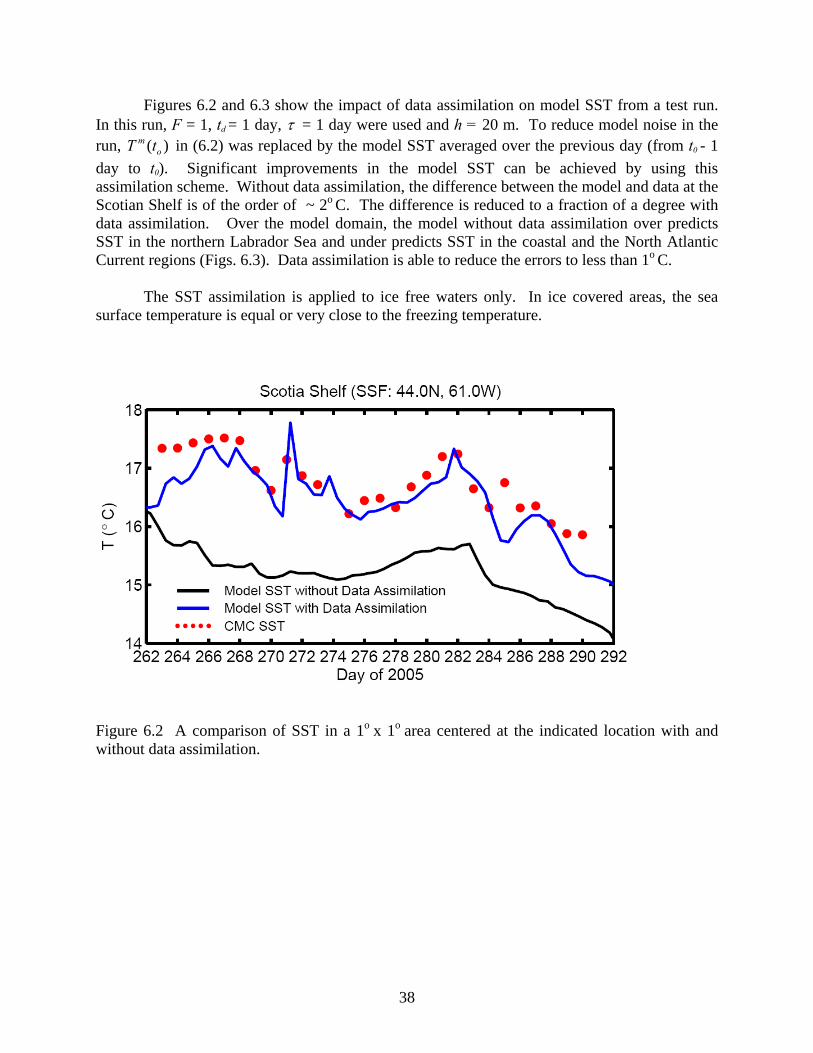
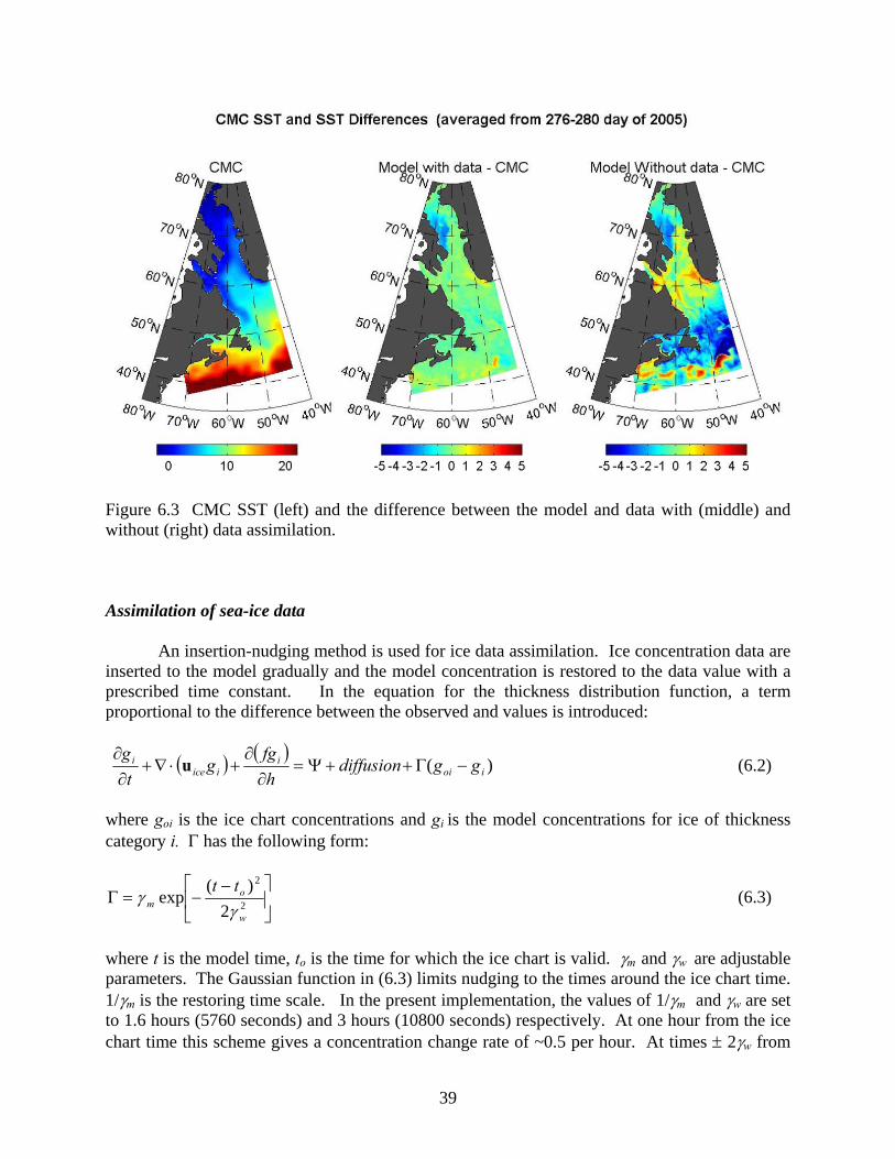
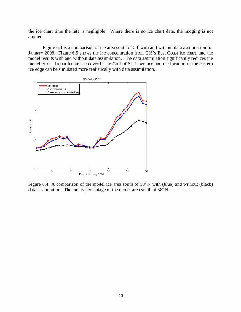
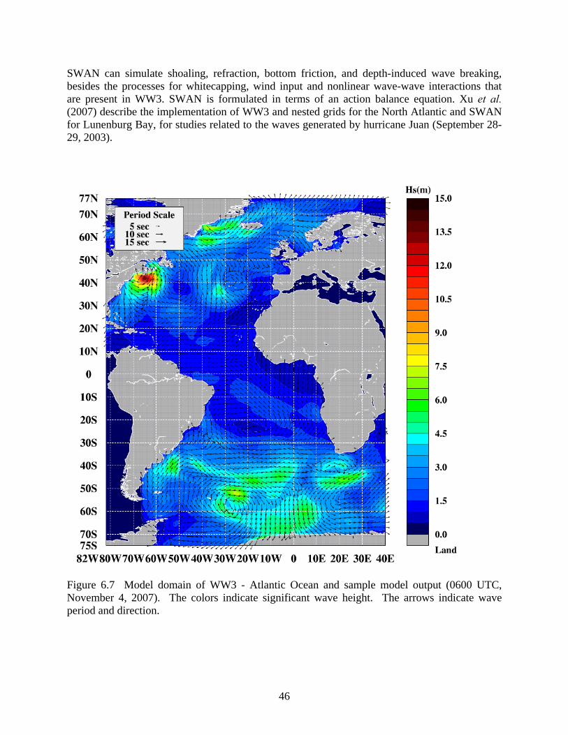
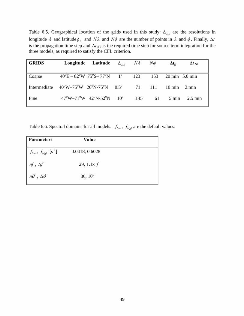