Better Together: Quantifying the Benefits of the Smart Network

©2013 Joe Weinman. All Rights Reserved.

Better Together: Quantifying the Benefits of the

Smart Network

Working Paper, March 3, 2013

Joe Weinman1

Permalink: http://www.joeweinman.com/Resources/SmartNetwork.pdf

Abstract

Three approaches to load balancing in a distributed computing network are evaluated analytically using

statistics and via Monte Carlo simulation: 1) random selection; 2) selection based solely on identifying

the server with the lowest response time; 3) selection based on identification of a combination of path

and server with the lowest total response time. Analytical and simulation results show that the lowest

expected response times occur via joint optimization. The exact improvement depends on the

underlying distributions of path response times and server response times. An exemplary case where

each path and server is an independent, identically distributed random variable with a continuous

uniform distribution on is assessed; then the improvement may be approximated by

√ , where is the number of alternative combinations of path and server. Generally, when

is a random variable representing path response times, the value of a smart network in reducing

response time is as . Such improvements support a philosophy of “smart”

networks vs. “dumb pipes.”

1. Introduction

In the late ‘90s, the world underwent a tectonic shift from circuit-switched POTS (Plain Old Telephone

Service) to everything over the Internet, as David Isenberg presciently foretold in “The Rise of the Stupid

Network1”. However, as I argued recently2, it isn’t clear any longer that “dumb pipes” and “stupid

networks” are the most performant architecture for distributed computing; better results can be

achieved for certain applications via global optimization across endpoints and networks. As we will

show, “intelligent networks,” —at least smart enough to provide status on congestion or response time

and quickly control the path that flows should take—can offer quantifiably superior performance that is

formally provable. Reduced response time generates business value, through, e.g., greater revenue,

reduced churn, and enhanced labor productivity3. Such networks occur in a variety of campus and wide

1 Joe Weinman leads Cloud Services and Strategy for Telx. The views expressed herein are his own. Contact

information is at http://www.joeweinman.com/contact.htm .

http://www.joeweinman.com/Resources/SmartNetwork.pdf

http://www.joeweinman.com/contact.htm

Better Together: Quantifying the Benefits of the Smart Network

© 2013 Joe Weinman. All Rights Reserved.

area network contexts, such as software-defined networks and OpenFlow4, but can even occur locally,

such as in the use of multi-path I/O, e.g., a switched fabric such as InfiniBand5. The general problem is

broader than computing, as in the selection of a particular coffee shop from among many based on the

wait for baristas and rush hour highway traffic. Abstractly, the problem is even broader than merely

response time, as in the selection of the least expensive vacation based both on airfare (transport

network) costs and hotel (on demand utility service) costs.

One key networked computing application is “anycasting,” where a client can be served from any of

several nodes. An example might be a search query, where the search index and query servers are

replicated in multiple geographic regions. Another might be eCommerce, where a product catalog page

can be delivered from anywhere, and a purchase transaction can be concluded anywhere. Yet another

example might be content delivery, where a given song or movie can be streamed from any of several

locations.

There are a number of approaches to selecting such a node, including random selection or round robin

approaches, which are intended to have the effect of load balancing, to load balancing based on server

load or recent response times, where a site is selected based on an expectation that it is in the best

position to take on additional work. However, an experimental system called “Aster*x” (formerly “Plug-

n-Serve6”) run at Stanford University by Nikhil Handigol, Nick McKeown, and their colleagues offers

tantalizing evidence7 that considering both network response times—which vary based on everything

from propagation delays to congestion in packet-switched networks—together with server response

times can offer the best performance. Moreover, Handigol points out8 that today’s reality is very

different: A CDN provider is likely to pick a node based on load, whereas an ISP is likely to pick a path

based on network congestion; the decisions are disjoint, and thus the performance is suboptimal.

We’ll quantify this and examine simulation results below, but for a preview, let’s briefly consider a

simple formulation. Let round-trip latencies on paths have distributions , where each is

an independent, identically distributed continuous random variable with

, and similarly let response times for servers be

characterized by independent, identically distributed continuous random variables , where

, and let response

times of various combinations of paths and servers follow . Then an algorithm that selects

combinations at random will have an expected response time of since the mean of the sum is

the sum of the means. One based on server-only selection without considering the path, i.e., a “stupid

network” approach, will have an expected value of , where is the first order statistic,

i.e., minimum, of a set of samples { } As approaches , the term approaches

, thus the total response time will never be better than However, an algorithm which

performs joint optimization has an expected total response time of . With such a “smart

network” approach, as , the expected total response time approaches . Except for

the trivial case of one server on one path where , the “smart network” approach always provides

better performance than the “stupid” one, and in the general case, the improvement is in

the limit as . Monte Carlo simulation results support the analysis.



2. A Simple Analogy

To understand qualitatively why joint optimization is better than server-only selection, let’s consider a

simple game of cards, where the lowest total face value for a pair of cards wins. Faced with the deal

shown in Figure 1, and with no additional information, the wisest course of action would be to pick the

pair that includes the six of diamonds, given that the expected value of each of the unseen cards is

identical and thus that choice offers the best odds of winning.

Figure 1: Playing Card Pair Selection with Partial Information

As it happens, however, if we could see the other cards, we would come to realize that the rightmost

pair is not the best selection. In fact, as can be seen in Figure 2, the six of diamonds is paired with the

ten of spades, making it the worst selection, with a total of 16, as opposed to the winning choice of the

pair comprising the eight of clubs and the three of hearts, with a winning low score of 11.



Figure 2: Playing Card Pair Selection with Complete Information

This card game is a metaphor for a distributed computing scenario, such as cloud computing or content

delivery. In the playing card example we are choosing a pair of cards, in the computing scenario we

need to choose a pair comprising a server and the path to that server, as shown in Figure 3. The path

may include one or more local area, metropolitan area, or wide area networks. The server is an

abstraction for a web server, database server, file server, etc., or combination of these and other

elements such as firewalls. The choices now have different values, but instead of face values, they are

now response times. We will consider network response time to be round trip latency.



Figure 3: A Distributed Computing Scenario with 4 Options

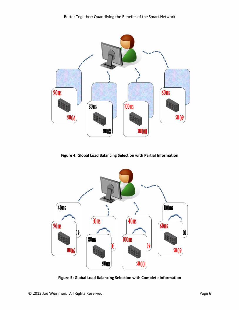
To relate this distributed computing example back to the playing card context, we can refer to Figure 4,

which shows us trying to make a decision of which combination of path and server to select based only

on the server data with no visibility into the network performance. As might be expected, the best

choice can only be made when we have complete information, as in Figure 5.



Figure 4: Global Load Balancing Selection with Partial Information

Figure 5: Global Load Balancing Selection with Complete Information



We could refer to only server data to do load balancing, but we can make a wiser decision when we use

both server and network data.

While more information in these examples led to a better solution, one might ask how much better the

solution is, and whether more options increases the quality of the solution. In other words, we can do

better both by turning the face down card face up, and by having more pairs of cards or servers and

paths to choose from.

3. Quantifying the Benefits of the Smart Network

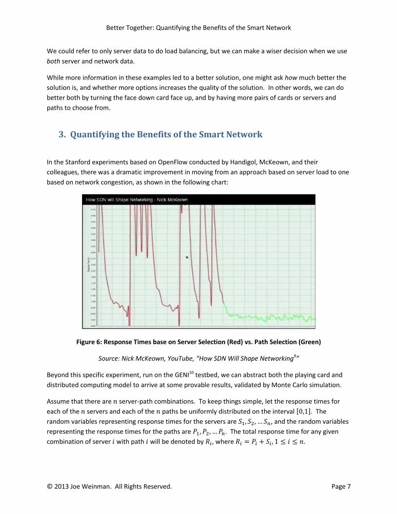
In the Stanford experiments based on OpenFlow conducted by Handigol, McKeown, and their

colleagues, there was a dramatic improvement in moving from an approach based on server load to one

based on network congestion, as shown in the following chart:

Figure 6: Response Times base on Server Selection (Red) vs. Path Selection (Green)

Source: Nick McKeown, YouTube, “How SDN Will Shape Networking9”

Beyond this specific experiment, run on the GENI10 testbed, we can abstract both the playing card and

distributed computing model to arrive at some provable results, validated by Monte Carlo simulation.

Assume that there are server-path combinations. To keep things simple, let the response times for

each of the servers and each of the paths be uniformly distributed on the interval . The

random variables representing response times for the servers are , and the random variables

representing the response times for the paths are . The total response time for any given

combination of server with path will be denoted by , where .



We can now evaluate three different algorithms for servicing a given user request.

Random Selection. If a combination of network path and server is selected at random, the expected

value of is This is because , since the

expected value of a uniformly distributed random variable—either or —on [0,1] is .5.

Server-Based Selection. The case of server-based selection is like the selection of a pair of playing cards

without seeing the value of the card that is face down. The expected value of the path, .

However, the expected value of the response time of the best server is a little bit trickier. If we only

have one server it is , but we may have several to choose from. The more servers we have to choose

from, the more likely it is that there will be a lower and lower value. In fact, it turns out that in this

exact case, based on the theory of order statistics, ( ) { }

.

Consequently, the expected value of is

( )

Joint Optimization. Suppose we try to optimize jointly based on the selecting one of the pairs. The

distribution of response times across both server and path may be characterized as a new random

variable which “encodes” the total of both and , i.e., . The sum of two independent

uniformly distributed random variables on is a random variable on that has a symmetric

triangular distribution. Using the formula11 derived by H. N. Nagaraja, a professor of Statistics,

Biostatistics, and Medicine and chair of the Division of Biostatistics at Ohio State University, and co-

author of the book Order Statistics12, but doubling the expected value for the min of a triangular

distribution on to arrive at one for a symmetric triangular distribution on we know that

{ } ∑ (

)

∑ (

)

{

}

Fortunately, this rather complex formula has been shown13 by Nagaraja to be approximately equal to

√ (after doubling the formula he provides for a triangular distribution on .)

4. Simulation Results

Simulation results bear this out. A Monte Carlo simulation, shown in Figure 7, was written14 in Javascript

to quantify the difference between a random algorithm, a server-only-based algorithm, and a joint

optimization algorithm, as the number of choices increases from 1 to 20.



Figure 7: ComplexModels.com Smart Networks Simulation,

As can be seen, the fastest total does not necessarily use the fastest path nor fastest server. The data

below (where 100 represents 1.0) are from 20 experiments (simulation runs), each of 10,000 trials.

Figure 8: Compilation of Simulation results for to

0

20

40

60

80

100

120

1 3 5 7 9 11 13 15 17 19

Joint Optimization

Server Only

Random



5. Observations

What do the simulation runs and the abstract analysis tell us?

1) When there is only one combination, there is no difference between the three strategies.

2) When there are two or more combinations to choose from, we can do better than random.

3) Except for the trivial case of only one combination, where there is no difference, the joint

optimization strategy is always better than the server-only strategy.

4) The server-only strategy flat-lines at the expected value of a randomly selected path.

5) The joint optimization strategy can go as low as we might desire…with an infinite number of

options, the expected value of the total response time is . Extrapolating the simulation results

shows this as well as considering the value of √ as .

6) Even with only a handful of options, there are substantial benefits to be gained from any kind of

optimization, but the joint optimization strategy is significantly better than merely making

decisions based on server loads.

6. Caveats

There are a few assumptions that are worth surfacing, lest too-broad conclusions be drawn.

1) One assumption is that server loads are independent of each other and independent of path

loads. To the extent that each given server only has one path to it and transactions have similar

characteristics, each server load and response time will be highly correlated with its

corresponding path load and response time. In today’s multi-carrier, multi-application

environment and mesh Internet architecture, they are likely to be independent, however.

2) Another assumption is that server response times and path response times are on par with one

another. To the extent that the server response times are much greater than path response

times, the network becomes insignificant. With today’s wide area cloud and ecommerce

transactions, however, it is not unusual to find both on the order of, say, 30 to 50 milliseconds,

and so this assumption is not unrealistic. In fact, one may find the reverse is true, where

embarrassingly parallel activities for, say, serving search queries have reduced the server-side

response time to such a low level that geographic dispersion to multiple service nodes is

required to bring the network latencies back into rough parity. Even then, network latencies



may be an order of magnitude or two greater than server response times, say, for keystroke

processing for progressive search.

3) We have assumed uniform distributions. The general logic still holds with different

distributions, although, to the extent that, say, response times are normally distributed with

extremely small standard deviations, response times would in effect be close to constant,

obviating the need for any such optimization.

4) We have assumed uniform distributions on . To the extent that the range and thus

standard deviation are small relative to the minimum (i.e., a low coefficient of variation), such

optimization becomes irrelevant. For example, if the range were optimization would

achieve a less than difference. The general form of and are on the interval [ , with

In fact, even if uniformly distributed, each path and server might have a different lower

and upper bound, i.e., (

)

, and so on. If, say,

, our algorithms don’t need to be very smart to determine that Path 1 is always best.

5) Decision cycle times are also important and short-term stability is important. The assumption is

that a selection of a path and server combination can be made quickly enough after

measurement of path and server response times to select the best combination. If by the time a

user transaction is routed to a selected combination the congestion or load of each element has

changed, we are for all intents and purposes making a random selection, not an intentional

optimizing one. Moreover, we are assuming that the problem is computationally tractable at

scale, and that “microflows” based on connections between particular clients and servers can be

maintained for the duration of a session and that deployment of rules defining selected options

can be successfully transitioned. Fortunately, Richard Wang, Dana Butnariu, and Jennifer

Rexford of Princeton University have shown15 that there are feasible algorithms for

“partitioning” and “transitioning” such traffic in suitable time frames.

6) We also have implicitly assumed that the selection of path does not create a “tragedy of the

commons” type of aggregate behavior. If enough user traffic was routed to the best-performing

route to make it the worst-performing route, results could be worse than if a route was selected

at random. The general notion of a software-defined network with logically centralized control

should prevent this.

Despite these caveats, however, results from the Stanford University study deployed on a real-world

test bed showed dramatic improvement by moving to a path-based approach from a server-based

approach, so the results would appear to have validity.



7. Conclusion

This analysis shows that subject to the assumptions, optimization decisions made by considering both

network and server behavior, with such routing applied to the network through various emerging

techniques such as Network as a Service, or Software Defined Networks such as OpenFlow, can improve

the end-user experience and/or performance of distributed applications. As the number of options

approaches infinity, a random selection remains mired at a response time of ; a server-

only-based algorithm can never do better than ; and a joint optimization solution

approaches a response time of { } , which is . We have focused on

the simplest case to analyze, where all random variables are uniformly distributed on , but subject

to the caveats, it should be apparent that the conclusions are broadly applicable and a consequence of

the fundamentals of order statistics, rather than any domain-specific characteristic. This suggests that

smart networks can offer better performance than “stupid” ones, in turn generating business value.

8. Acknowledgment

I cannot thank H. N. Nagaraja (http://www.stat.osu.edu/~hnn/) enough for his extremely responsive and

thoughtful replies to a request arriving out of the blue to characterize the order statistics for the

triangular distribution, a surprisingly complex problem as can be surmised by Section 3.

9. References 1 David Isenberg, “The Rise of the Stupid Network,” Computer Telephony, August 1997, pp. 16-26.

http://isen.com/stupid.html. 2 Joe Weinman, “Why the ‘Stupid Network’ Isn’t Our Destiny After All,” GigaOM.com, Dec. 15, 2012.

http://gigaom.com/2012/12/15/why-the-stupid-network-isnt-our-destiny-after-all/. 3 Joe Weinman, Cloudonomics: The Business Value of Cloud Computing, John Wiley & Sons, 2012.

4 Nick McKeown, Tom Anderson, Hari Balakrishnan, Guru Parulkar, Larry Peterson, Jennifer Rexford, Scott Shenker,

and Jonathan Turner, “OpenFlow: Enabling Innovation in Campus Networks,” ACM SIGCOMM Computer Communication Review, 38(2):69–74, April 2008. http://ccr.sigcomm.org/online/files/p69-v38n2n-mckeown.pdf. 5 Bob Rizika, “InfiniBand—A Great Cloud Computing Network Interconnect,” ProfitBricks Blog, September 7, 2012.

http://blog.profitbricks.com/infiniband-a-great-cloud-computing-network-interconnect/. 6 Nikhil Handigol, Srinivasan Seetharaman, Nick McKeown, and Ramesh Johari, “Plug-n-Serve: Load-Balancing Web

Traffic using OpenFlow,” http://conferences.sigcomm.org/sigcomm/2009/demos/sigcomm-pd-2009-final26.pdf. 7 Nikhil Handigol, Srini Seetharaman, Mario Flajslik, Aaron Gember, Nick McKeown, Guru Parulkar, Aditya Akella,

Nick Feamster, Russ Clark, Arvind Krishnamurthy, Vjekoslav Brajkovic, and Tom Anderson, “Aster*x: Load-Balancing Web Traffic over Wide-Area Networks.” http://www.stanford.edu/~nikhilh/pubs/handigol-gec9.pdf. 8 Nikhil Handigol, “Should a Load Balancer Choose the Path as Well as the Server?,” May, 2011.

http://www.mvdirona.com/jrh/TalksAndPapers/Handigol-Amazon-May2011.pdf. 9 Nick McKeown, “How SDN Will Shape Networking,” YouTube.com. http://www.youtube.com/watch?v=c9-

K5O_qYgA. 10

http://www.geni.net/

http://isen.com/stupid.html

http://gigaom.com/2012/12/15/why-the-stupid-network-isnt-our-destiny-after-all/

http://ccr.sigcomm.org/online/files/p69-v38n2n-mckeown.pdf

http://blog.profitbricks.com/infiniband-a-great-cloud-computing-network-interconnect/

http://conferences.sigcomm.org/sigcomm/2009/demos/sigcomm-pd-2009-final26.pdf

http://www.stanford.edu/~nikhilh/pubs/handigol-gec9.pdf

http://www.mvdirona.com/jrh/TalksAndPapers/Handigol-Amazon-May2011.pdf

http://www.youtube.com/watch?v=c9-K5O_qYgA

http://www.youtube.com/watch?v=c9-K5O_qYgA

http://www.geni.net/



11

H. N. Nagaraja, “Expected Value of the Sample Minimum From a Triangular Distribution,” February 27, 2013, personal communication. 12

David, H. A. and Nagaraja, H. N., Order Statistics, Third Edition, Wiley, N.J., 2003. 13

H. N. Nagaraja, “Moments of the Sample Minimum from the Triangular Distribution,” March 2, 2013, personal communication. 14

Joe Weinman, http://www.complexmodels.com/SmartNetwork.htm. 15

Richard Wang, Dana Butnariu, and Jennifer Rexford , “OpenFlow-Based Server Load Balancing Gone Wild.” http://static.usenix.org/event/hotice11/tech/full_papers/Wang_Richard.pdf.

http://www.complexmodels.com/SmartNetwork.htm

http://static.usenix.org/event/hotice11/tech/full_papers/Wang_Richard.pdf

Better Together: Quantifying the Benefits of the Smart Network

Documents

Transcript of Better Together: Quantifying the Benefits of the Smart Network