Benders DecompositionOperations Research

Anthony Papavasiliou

1 / 35

Contents

1 Context and Description of the Algorithm

2 Useful Results

3 Statement of Algorithm and Proof of Convergence

4 Example: Capacity Expansion Planning

2 / 35

Table of Contents

1 Context and Description of the Algorithm

2 Useful Results

3 Statement of Algorithm and Proof of Convergence

4 Example: Capacity Expansion Planning

3 / 35

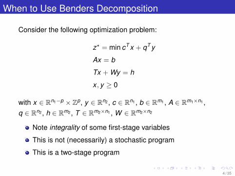
When to Use Benders Decomposition

Consider the following optimization problem:

z? = min cT x + qT y

Ax = b

Tx + Wy = h

x , y ≥ 0

with x ∈ Rn1−p × Zp, y ∈ Rn2 , c ∈ Rn1 , b ∈ Rm1 , A ∈ Rm1×n1 ,q ∈ Rn2 , h ∈ Rm2 , T ∈ Rm2×n1 , W ∈ Rm2×n2

Note integrality of some first-stage variables

This is not (necessarily) a stochastic program

This is a two-stage program

4 / 35

Context for Benders decomposition:

1 entire problem is difficult to solve

2 if Tx + Wy = h is ignored, problem is relatively easy

3 if x is fixed, problem is relatively easy

5 / 35

Idea of Benders Decomposition

Define value function V : Rn1 → R

(S) : V (x) = miny

qT y

Wy = h − Tx

y ≥ 0

Equivalent description of problem

min cT x + V (x)

Ax = b

x ∈ dom V

x ≥ 0

Note: dom V = {x : ∃y ,Tx + Wy = h}6 / 35

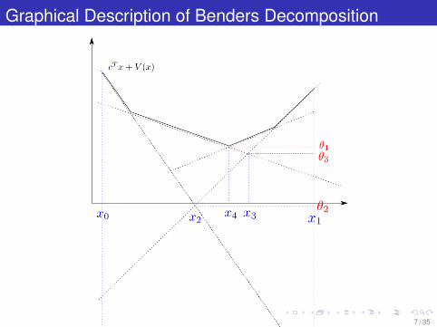
Graphical Description of Benders Decomposition

7 / 35

Table of Contents

1 Context and Description of the Algorithm

2 Useful Results

3 Statement of Algorithm and Proof of Convergence

4 Example: Capacity Expansion Planning

8 / 35

Dual of Second-Stage Linear Program

The dual of (S) can be expressed as:

(D) : maxπ

πT (h − Tx)

πT W ≤ qT

Note: feasible region of (D) does not depend on x

V : set of extreme points of πT W ≤ qT

R: set of extreme rays of πT W ≤ qT

9 / 35

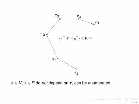
π ∈ V , σ ∈ R do not depend on x , can be enumerated

10 / 35

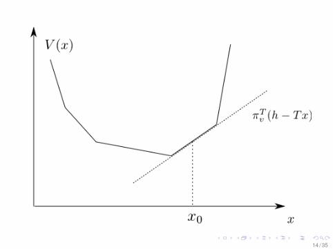
Value Function Is Piecewise Linear

V (x) is a piecewise linear convex function of x

If πv are dual optimal multipliers of (S) given x0, then

πTv (h − Tx0)

is a supporting hyperplane of V (x) at x0

We recall a previous result for the proof

11 / 35

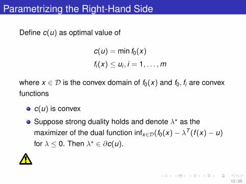
Parametrizing the Right-Hand Side

Define c(u) as optimal value of

c(u) = min f0(x)

fi(x) ≤ ui , i = 1, . . . ,m

where x ∈ D is the convex domain of f0(x) and f0, fi are convexfunctions

c(u) is convex

Suppose strong duality holds and denote λ? as themaximizer of the dual function infx∈D(f0(x)− λT (f (x)− u)

for λ ≤ 0. Then λ? ∈ ∂c(u).

12 / 35

From previous result:

V (h − Tx) is convex, so V (x) is convex

πv ∈ ∂V (h − Tx0), so πTv (h − Tx) is a supporting

hyperplane of V (x) at x0

(S) has a finite number of dual optimal multipliers⇒ finitenumber of supporting hyperplanes for V (x)⇒ V (x) ispiecewise linear convex

13 / 35

14 / 35

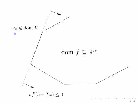
Domain of Value Function

dom V can be expressed equivalently as follows:

dom V = {σTr (h − Tx) ≤ 0, σr ∈ R}

where σr , r ∈ R is the set of extreme rays of πT W ≤ qT

15 / 35

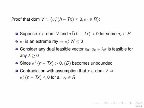
Proof that dom V ⊆ {σTr (h − Tx) ≤ 0, σr ∈ R}:

Suppose x ∈ dom V and σTr (h − Tx) > 0 for some σr ∈ R

σr is an extreme ray⇒ σTr W ≤ 0

Consider any dual feasible vector π0: π0 + λσ is feasible forany λ ≥ 0

Since σTr (h − Tx) > 0, (D) becomes unbounded

Contradiction with assumption that x ∈ dom V ⇒σT

r (h − Tx) ≤ 0 for all σr ∈ R

16 / 35

Proof that {σTr (h − Tx) ≤ 0, σr ∈ R} ⊆ dom V :

Any ray of πT W ≤ qT can be expressed as convexcombination of extreme rays

Therefore, for any ray σ of πT W ≤ qT it follows thatσT (h − Tx) ≤ 0⇒ (D) cannot become unbounded

17 / 35

18 / 35

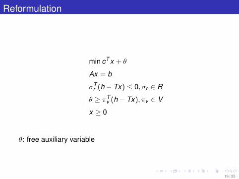
Reformulation

min cT x + θ

Ax = b

σTr (h − Tx) ≤ 0, σr ∈ R

θ ≥ πTv (h − Tx), πv ∈ V

x ≥ 0

θ: free auxiliary variable

19 / 35

Master Problem

Relax inequalities that define V (x) and dom V :

(M) : zk = min cT x + θ

Ax = b

σTr (h − Tx) ≤ 0, σr ∈ Rk ⊆ R

θ ≥ πTv (h − Tx), πv ∈ Vk ⊆ V

x ≥ 0

20 / 35

Bounds and Exchange of Information

Solution of master problem provides:

lower bound zk ≤ z?

candidate solution xk

under-estimator of V (xk ), θk ≤ V (xk )

Solution of slave problem with input xk provides:

upper bound cT xk + qT yk+1 ≥ z?

new vertex πk+1 or new extreme ray σk+1

21 / 35

Table of Contents

1 Context and Description of the Algorithm

2 Useful Results

3 Statement of Algorithm and Proof of Convergence

4 Example: Capacity Expansion Planning

22 / 35

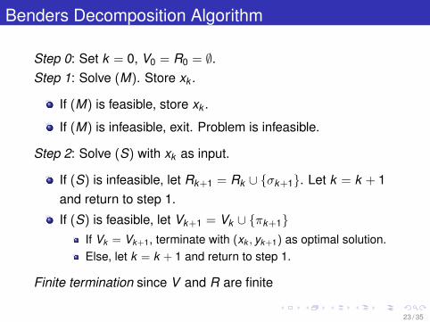
Benders Decomposition Algorithm

Step 0: Set k = 0, V0 = R0 = ∅.Step 1: Solve (M). Store xk .

If (M) is feasible, store xk .

If (M) is infeasible, exit. Problem is infeasible.

Step 2: Solve (S) with xk as input.

If (S) is infeasible, let Rk+1 = Rk ∪ {σk+1}. Let k = k + 1and return to step 1.

If (S) is feasible, let Vk+1 = Vk ∪ {πk+1}If Vk = Vk+1, terminate with (xk , yk+1) as optimal solution.Else, let k = k + 1 and return to step 1.

Finite termination since V and R are finite

23 / 35

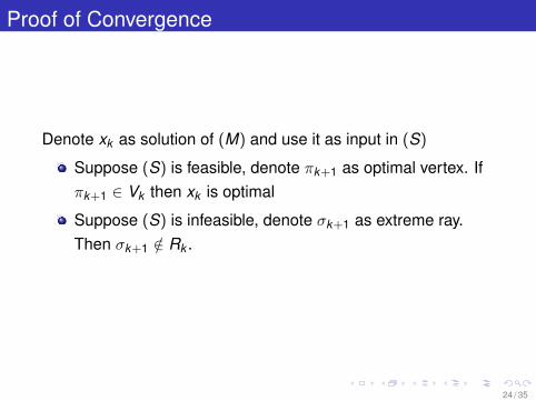
Proof of Convergence

Denote xk as solution of (M) and use it as input in (S)

Suppose (S) is feasible, denote πk+1 as optimal vertex. Ifπk+1 ∈ Vk then xk is optimal

Suppose (S) is infeasible, denote σk+1 as extreme ray.Then σk+1 /∈ Rk .

24 / 35

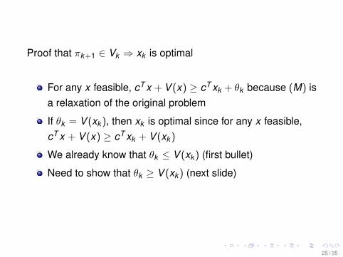
Proof that πk+1 ∈ Vk ⇒ xk is optimal

For any x feasible, cT x + V (x) ≥ cT xk + θk because (M) isa relaxation of the original problem

If θk = V (xk ), then xk is optimal since for any x feasible,cT x + V (x) ≥ cT xk + V (xk )

We already know that θk ≤ V (xk ) (first bullet)

Need to show that θk ≥ V (xk ) (next slide)

25 / 35

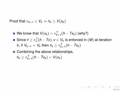
Proof that πk+1 ∈ Vk ⇒ θk ≥ V (xk )

We know that V (xk ) = πTk+1(h − Txk ) (why?)

Since θ ≥ πTv (h− Tx), v ∈ Vk is enforced in (M) at iteration

k , if Vk+1 = Vk then θk ≥ πTk+1(h − Txk )

Combining the above relationships,θk ≥ πT

k+1(h − Txk ) = V (xk )

26 / 35

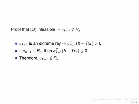
Proof that (S) infeasible⇒ σk+1 /∈ Rk

σk+1 is an extreme ray⇒ σTk+1(h − Txk ) > 0

If σk+1 ∈ Rk , then σTk+1(h − Txk ) ≤ 0

Therefore, σk+1 /∈ Rk

27 / 35

Table of Contents

1 Context and Description of the Algorithm

2 Useful Results

3 Statement of Algorithm and Proof of Convergence

4 Example: Capacity Expansion Planning

28 / 35

Load Duration Curve

Load duration curve is obtained by sorting load time series indescending order

29 / 35

Mathematical Programming Formulation

minx ,y≥0

n∑i=1

(Ii · xi +m∑

j=1

Ci · Tj · yij)

s.t.n∑

i=1

yij = Dj , j = 1, . . . ,m

m∑j=1

yij ≤ xi , i = 1, . . .n

Ii ,Ci : fixed/variable cost of technology i

Dj ,Tj : height/width of load block j

yij : capacity of i allocated to j

xi : capacity of i

30 / 35

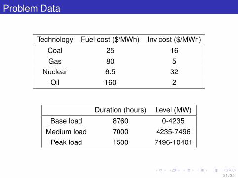
Problem Data

Technology Fuel cost ($/MWh) Inv cost ($/MWh)Coal 25 16Gas 80 5

Nuclear 6.5 32Oil 160 2

Duration (hours) Level (MW)Base load 8760 0-4235

Medium load 7000 4235-7496Peak load 1500 7496-10401

31 / 35

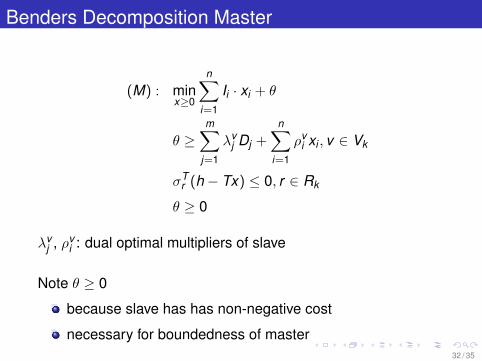
Benders Decomposition Master

(M) : minx≥0

n∑i=1

Ii · xi + θ

θ ≥m∑

j=1

λvj Dj +

n∑i=1

ρvi xi , v ∈ Vk

σTr (h − Tx) ≤ 0, r ∈ Rk

θ ≥ 0

λvj , ρv

i : dual optimal multipliers of slave

Note θ ≥ 0

because slave has has non-negative cost

necessary for boundedness of master32 / 35

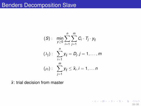
Benders Decomposition Slave

(S) : miny≥0

n∑i=1

m∑j=1

Ci · Tj · yij

(λj) :n∑

i=1

yij = Dj , j = 1, . . . ,m

(ρi) :m∑

j=1

yij ≤ x̄i , i = 1, . . .n

x̄ : trial decision from master

33 / 35

Sequence of Investments

Iteration Coal (MW) Gas (MW) Nuclear (MW) Oil (MW)1 0 0 0 02 0 0 0 8735.63 0 0 0 18565.14 0 14675.8 0 05 10673.3 0 0 06 0 0 7337.9 3063.17 0 1497.7 7337.9 732.28 0 1497.7 7337.9 2033.39 0 0 8966 1435

10 2851.8 2187.2 5362 011 8321 0 0 208012 6989.5 4489.5 56.5 013 3261 2905 4235 0

34 / 35

Observations

A new investment proposal is necessarily made in eachiteration (why?)

Greedy behaviorFirst iteration: no investmentEarly iterations: technologies with low investment cost

35 / 35