Belief Propagation in a 3D Spatio-temporal MRF for Moving Object Detection

Zhaozheng Yin and Robert CollinsDepartment of Computer Science and Engineering

The Pennsylvania State University, University Park, PA 16802{zyin,rcollins}@cse.psu.edu

Abstract

Previous pixel-level change detection methods eithercontain a background updating step that is costly for mov-ing cameras (background subtraction) or can not locate ob-ject position and shape accurately (frame differencing). Inthis paper we present a Belief Propagation approach formoving object detection using a 3D Markov Random Field(MRF) model. Each hidden state in the 3D MRF model rep-resents a pixel’s motion likelihood and is estimated usingmessage passing in a 6-connected spatio-temporal neigh-borhood. This approach deals effectively with difficult mov-ing object detection problems like objects camouflaged bysimilar appearance to the background, or objects with uni-form color that frame difference methods can only par-tially detect. Three examples are presented where movingobjects are detected and tracked successfully while han-dling appearance change, shape change, varied movingspeed/direction, scale change and occlusion/clutter.

1. IntroductionBelief Propagation (BP) has emerged as a powerful tool

to solve early vision problems such as stereo, optical flowand image restoration using MRF models [4] [6]. Somepopular inference algorithms to approximate the best esti-mate of each node in the MRF model are developed andcompared in [13] [14]. In this paper we present a 3D MRFmodel for detecting moving objects in video streams, anda BP algorithm for approximate inference under this model(Fig.1). This approach overcomes the deficiencies of somecommon pixel-level change detection methods.

Previous pixel-level change detection methods such asbackground subtraction, inter-frame differencing and three-frame differencing are widely used [2] [8] [10]. Back-ground subtraction relies on a background model for com-parison, but adaptive background updating is costly for amoving camera. With stationary cameras, inter-frame dif-ferencing easily detects motion but does a poor job of lo-calizing the object (usually only parts of the object are de-

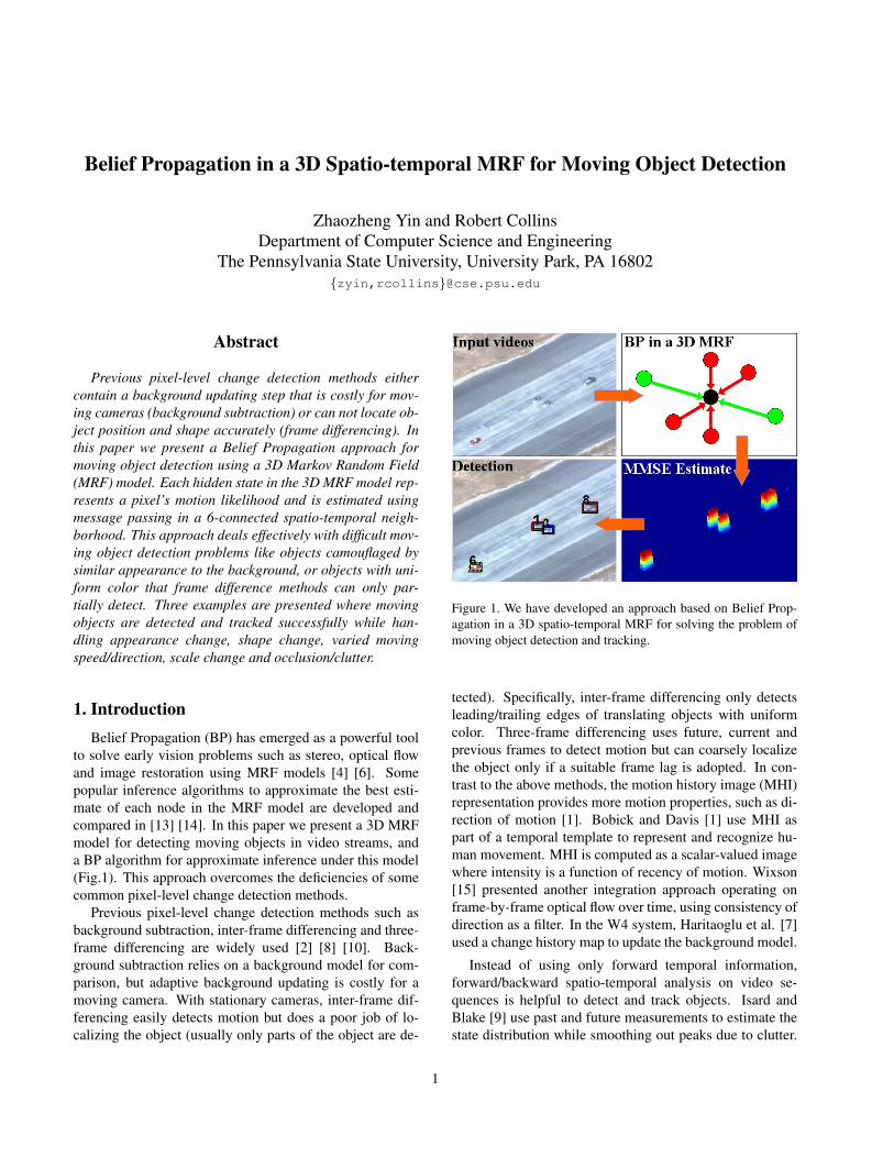
Figure 1. We have developed an approach based on Belief Prop-agation in a 3D spatio-temporal MRF for solving the problem ofmoving object detection and tracking.

tected). Specifically, inter-frame differencing only detectsleading/trailing edges of translating objects with uniformcolor. Three-frame differencing uses future, current andprevious frames to detect motion but can coarsely localizethe object only if a suitable frame lag is adopted. In con-trast to the above methods, the motion history image (MHI)representation provides more motion properties, such as di-rection of motion [1]. Bobick and Davis [1] use MHI aspart of a temporal template to represent and recognize hu-man movement. MHI is computed as a scalar-valued imagewhere intensity is a function of recency of motion. Wixson[15] presented another integration approach operating onframe-by-frame optical flow over time, using consistency ofdirection as a filter. In the W4 system, Haritaoglu et al. [7]used a change history map to update the background model.

Instead of using only forward temporal information,forward/backward spatio-temporal analysis on video se-quences is helpful to detect and track objects. Isard andBlake [9] use past and future measurements to estimate thestate distribution while smoothing out peaks due to clutter.

1

Luthon et al. [12] propose an energy minimization strat-egy in the spatio-temporal domain for object detection andbuild a data pyramid by 3D low-pass filtering and 3D sub-sampling. To find the minimum of the energy function, a de-terministic relaxation algorithm ICM (Iterated ConditionalModes) is used.

With the realization that each pixel influences neighbor-ing pixels spatially and temporally in the video sequence,we develop a 3D MRF model to represent the system. Eachpixel has a hidden state node and an observed data node(e.g. inter-frame differencing result). Each state node has6-connected neighboring nodes: four 4-connected spatialones and 2 temporal ones (past and future). We apply theBelief Propagation algorithm to estimate the current stateby spatio-temporal message passing. Spatially we performloopy Belief Propagation [16] on each 2D frame grid. Tem-porally we perform 1D forward/backward BP for each pixelwithin a sliding temporal window. The intermediate resultsof our approach bear a strong resemblance to MHI repre-sentations, for example leaving a “trail” behind the mov-ing object. However the best estimate by forward/backwardspatio-temporal BP is much smoother than MHI, becauseour approach uses more (6-connected) neighbors for mes-sage passing than forward MHI (only the past temporalneighbor is used).

We first derive the 3D MRF model in Section 2. BeliefPropagation is discussed in Section 3. To illustrate the ef-fectiveness of this approach, we test it on challenging mov-ing object detection cases containing camouflaged objectsand objects with uniform color that are only partially de-tected by frame differencing. In Section 4 several track-ing examples are presented where moving object detectionis used to track vehicles. The tracking examples illustratethe algorithm’s performance in the presence of appearancechange, shape change, varied moving speed/direction, scalechange and occlusion/clutter.

2. Markov Random Field ModelMarkov chains defined in the time domain, e.g. Hidden

Markov Models (HMM), are often used to perform sequen-tial analysis. We note that a moving object covers a volumein the (x,y,t) space, and therefore use 3D Markov RandomFields for analyzing image sequences in the spatio-temporaldomain to detect moving objects (Fig.2).

The problem of detecting moving objects in the currentimage is equivalent to determining whether each pixel is oris not a motion pixel based on the given video observations.In other words, we need to estimate each pixel’s motionlikelihood state, given observed image data. Belief Prop-agation is a powerful algorithm for making approximate in-ferences over joint distributions defined by MRF models.

Using the 3D spatio-temporal MRF model, pixel (m,n)at time instant k has a hidden state node s(m,n, k) (cen-

Figure 2. 3D lattice defining the neighbors of a pixel.

ter black node in Fig.2) and a corresponding data noded(m,n, k). The network consists of nodes connected byedges that indicate conditional dependency. The statenode s(m,n, k) has a 3D neighborhood involving sixspatio-temporal interactions. In the spatial domain, nodes(m,n, k) has four-connected spatial neighbors: s(m ±1, n, k) and s(m,n ± 1, k). In the time domain, nodes(m,n, k) has two nearest temporal neighbors: s(m,n, k±1), which correspond to the past time instant k−1 and futuretime instant k + 1 separately. The design of these cliquesand nodes is described in Section 3.1. This spatio-temporalMRF model satisfies the 1st-order Markov characteristics—state node s(m,n, k) only interacts with its neighboringnodes, i.e. the state of node s(m,n, k) is determined ifits corresponding data node, four spatial neighboring statenodes and two temporal neighboring state nodes are known.Since the neighborhood of a pixel in the current frame in-cludes future frames, it is a bilateral MRF model and intro-duces a fixed lag in the detection system.

3. Belief PropagationThe above model contains only pairwise cliques, and the

joint probability over the 3D volume is

P (s1, ..., sN , d1, ...dN ) =∏i 6=j

ψij(si, sj)∏k

φk(sk, dk)

(1)where si and di represent state node and data node sepa-rately. ψ is the state transition function between a pair ofdifferent hidden state nodes and φ is the measurement func-tion between the hidden state node and observed data node.N represents the total number of state or data nodes in the3D volume. Under the squared loss function, the best es-timate for node sj is the mean of the posterior marginalprobability (minimum mean squared error estimate, MMSEestimate):

sjMMSE =∑sj

sj

∑si,i 6=j

P (s1, ..., sN , d1, ...dN ) (2)

where the inner sum gives the marginal distribution of sj .

Figure 3. (a) Computing belief; (b) Computing message.

Since the joint probability involves all the hidden statenodes and data nodes in the 3D volume, it is hard tocompute the MMSE estimate based on the implicit multi-variable probability distribution. However belief propaga-tion messages are effective to compute the MMSE estimaterecursively. Each hidden state node has a belief, which isa probability distribution defining the node’s motion likeli-hood. Thus the MMSE estimate of one node is computedas

sjMMSE =∑sj

sjb(sj) (3)

whereb(sj) = φj(sj , dj)

∏k∈Neighbor(j)

Mkj (4)

is the belief at node sj and k runs over all neighboringhidden state nodes of node sj . The belief at node sj isthe product of all the incoming messages (Mk

j ) and the lo-cal observed data message (φj(sj , dj)). The computationis shown in Fig.3(a). The passed messages specify whatdistribution each node thinks its neighbors should have.Fig.3(b) shows how to compute the message from node sk

to sj :

Mkj =

∑sk

ψjk(sj , sk)b(sk) (5)

After substituting b(sk) by Eq.4, we have

Mkj =

∑sk

ψjk(sj , sk)φk(sk, dk)∏

i∈Neighbor(k)\j

M ik (6)

where i ∈ Neighbor(k)\j denotes all the neighboring nodesof k other than j. After multiplying all the incoming mes-sages (M i

k) from neighboring nodes (except from the nodesj) and the observed data message (φk(sk, dk)), the productis evolved from the message-sender to the message-receiverby transition function ψjk(sj , sk).

3.1. Compatibility Function Selection

The hidden state sj represents the likelihood that a pixelcontains object motion, and its corresponding observationdata dj represents the binary motion detection result com-puted by inter-frame differencing at that time instant. Wecoarsely quantize each node’s belief and incoming/outgoingmessages into C buckets (C ≥ 2) and describe them as adiscrete probability mass function over [1, C].φj(sj , dj) describes the measurement relation (data

clique in Fig.2) between observation dj and hidden statenode sj . If dj equals zero, no motion is detected at thispixel by inter-frame differencing, and a uniform distribu-tion is used to represent “no-motion”. However, when dj

equals one, i.e. motion is definitely detected by inter-framedifferencing at this pixel, sj has an impulse distribution atsj = C to show the confidence of existing motion regard-less of what messages are passed to the node. Let sp

j denotethe pth state candidate at node sj (p ∈ [1, C]), the compati-bility function between observation and hidden state is

φj(spj , dj) =

{1C if dj = 0δ(sp

j = C) if dj = 1(7)

Currently we make “hard” decisions on the data term. A“soft” frame-differencing threshold for determining motioncould also be explored, i.e. the larger the intensity differ-ence between pixels in two frames, the more likely thatpixel is moving.ψij(si, sj) defines a state transition function (spa-

tial/temporal cliques in Fig.2) between two neighboringnodes via the Potts model:

ψij(spi , s

qj) =

{θ if p = q

ε otherwise(8)

where 0 < θ < 1, ε = (1 − θ)/(C − 1) and θ � ε.This compatibility function encourages neighboring nodesto have the same states. It also acts as a decay functionto reduce the motion likelihood in the absence of currentintensity differences. A pixel is NOT exactly as likely tomove as its neighbors, since the Potts model introduces thedecay term θ. Spatial cliques and temporal cliques couldhave different θ values, but in our testing, we use the samecompatibility function for both.

3.2. Message Computation

Fig.4 shows a 1D example to compute messages in termsof matrix operations. The message from observed data noded2 is a vector of C elements based on Eq.7:

φ2(s2, d2) =

{[ 1C . . . 1

C ]T if d2 = 0[0 . . . 0 1]T if d2 = 1

(9)

Figure 5. Test on the synthesized video sequence.

Figure 6. MMSE estimates of random patch by different kinds of BP with θ = 0.7 and C = 10.

Figure 4. 1D message computation example with C = 2.

The state transition is a C-by-C compatibility matrixbased on the Potts model of Eq.8:

Ψ =

θ ε . . . εε θ . . . ε...

. . . . . ....

ε . . . ε θ

(10)

The belief at node s2 (C element vector) is computed byEq.4:

b(s2) = φ2(s2, d2)·M12 (11)

where ‘·’ represents the element-wise product of two vec-tors. The message from node s2 to s3 is computed by Eq.6(matrix multiplication does the marginal sum):

M23 = Ψ ∗ b(s2) = Ψ ∗ (φ2(s2, d2)·M1

2 ) (12)

3.3. Message Update Schedule

To illustrate the effects of different message passingschedules, we use a synthesized image sequence as shownin Fig.5(a): the background is a 100*100 random map(each pixel has a uniform random intensity value within[0, 255]) and the moving object is a 10*10 random patch.It is hard for an appearance-based detector (e.g. histogrambased detector) to detect the camouflaged object, but ourforward/backward spatio-temporal BP algorithm easily de-tects object motion as shown in Fig.5(g). Based on the ob-served inter frame difference data (Fig.5(b)), a median filter(Fig.5(c)) or Gaussian filter (Fig.5(d-f)) can not recover thewhole moving object well. The median filter removes manyisolated detected motion pixels resulting in an object maskthat is too small. Gaussian filters are rotationally symmet-ric low pass filters. They blur the differenced image, anddifferent Gaussian window sizes and variance values causedifferent blur effects (thus prior knowledge about the objectsize is needed). Neither median filter nor Gaussian filterslocalize the object position accurately in Fig.5(c-f).

Each state node in our 3D MRF model has 6-connectedneighbors (two temporal and four spatial ones). There arenumerous ways to update the node’s belief and schedule itsmessage passing (Fig.6). For each frame (2D spatial gridgraph), we perform asynchronous accelerated message up-dating [14]. Four 1-dimensional BP sweeps (left to right,up to down, right to left, and down to up) are performed in-dividually and in parallel as shown in Fig.7. Here 1D BP

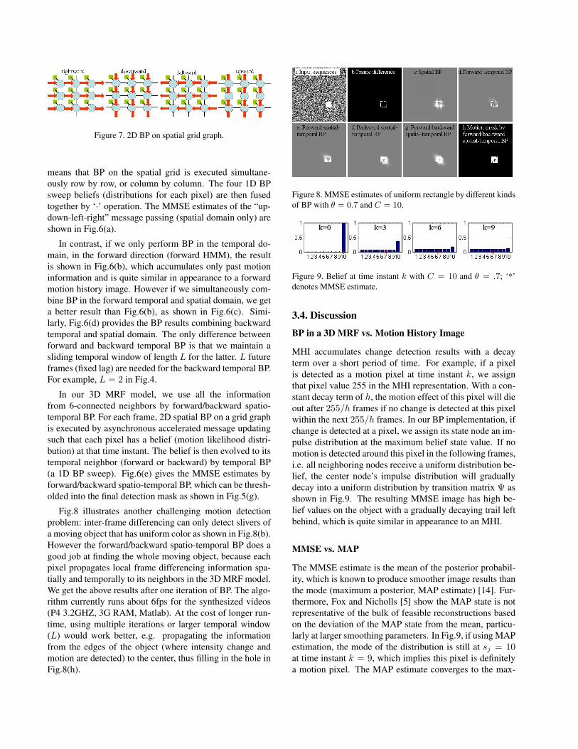
Figure 7. 2D BP on spatial grid graph.

means that BP on the spatial grid is executed simultane-ously row by row, or column by column. The four 1D BPsweep beliefs (distributions for each pixel) are then fusedtogether by ‘·’ operation. The MMSE estimates of the “up-down-left-right” message passing (spatial domain only) areshown in Fig.6(a).

In contrast, if we only perform BP in the temporal do-main, in the forward direction (forward HMM), the resultis shown in Fig.6(b), which accumulates only past motioninformation and is quite similar in appearance to a forwardmotion history image. However if we simultaneously com-bine BP in the forward temporal and spatial domain, we geta better result than Fig.6(b), as shown in Fig.6(c). Simi-larly, Fig.6(d) provides the BP results combining backwardtemporal and spatial domain. The only difference betweenforward and backward temporal BP is that we maintain asliding temporal window of length L for the latter. L futureframes (fixed lag) are needed for the backward temporal BP.For example, L = 2 in Fig.4.

In our 3D MRF model, we use all the informationfrom 6-connected neighbors by forward/backward spatio-temporal BP. For each frame, 2D spatial BP on a grid graphis executed by asynchronous accelerated message updatingsuch that each pixel has a belief (motion likelihood distri-bution) at that time instant. The belief is then evolved to itstemporal neighbor (forward or backward) by temporal BP(a 1D BP sweep). Fig.6(e) gives the MMSE estimates byforward/backward spatio-temporal BP, which can be thresh-olded into the final detection mask as shown in Fig.5(g).

Fig.8 illustrates another challenging motion detectionproblem: inter-frame differencing can only detect slivers ofa moving object that has uniform color as shown in Fig.8(b).However the forward/backward spatio-temporal BP does agood job at finding the whole moving object, because eachpixel propagates local frame differencing information spa-tially and temporally to its neighbors in the 3D MRF model.We get the above results after one iteration of BP. The algo-rithm currently runs about 6fps for the synthesized videos(P4 3.2GHZ, 3G RAM, Matlab). At the cost of longer run-time, using multiple iterations or larger temporal window(L) would work better, e.g. propagating the informationfrom the edges of the object (where intensity change andmotion are detected) to the center, thus filling in the hole inFig.8(h).

Figure 8. MMSE estimates of uniform rectangle by different kindsof BP with θ = 0.7 and C = 10.

Figure 9. Belief at time instant k with C = 10 and θ = .7; ‘*’denotes MMSE estimate.

3.4. Discussion

BP in a 3D MRF vs. Motion History Image

MHI accumulates change detection results with a decayterm over a short period of time. For example, if a pixelis detected as a motion pixel at time instant k, we assignthat pixel value 255 in the MHI representation. With a con-stant decay term of h, the motion effect of this pixel will dieout after 255/h frames if no change is detected at this pixelwithin the next 255/h frames. In our BP implementation, ifchange is detected at a pixel, we assign its state node an im-pulse distribution at the maximum belief state value. If nomotion is detected around this pixel in the following frames,i.e. all neighboring nodes receive a uniform distribution be-lief, the center node’s impulse distribution will graduallydecay into a uniform distribution by transition matrix Ψ asshown in Fig.9. The resulting MMSE image has high be-lief values on the object with a gradually decaying trail leftbehind, which is quite similar in appearance to an MHI.

MMSE vs. MAP

The MMSE estimate is the mean of the posterior probabil-ity, which is known to produce smoother image results thanthe mode (maximum a posterior, MAP estimate) [14]. Fur-thermore, Fox and Nicholls [5] show the MAP state is notrepresentative of the bulk of feasible reconstructions basedon the deviation of the MAP state from the mean, particu-larly at larger smoothing parameters. In Fig.9, if using MAPestimation, the mode of the distribution is still at sj = 10at time instant k = 9, which implies this pixel is definitelya motion pixel. The MAP estimate converges to the max-

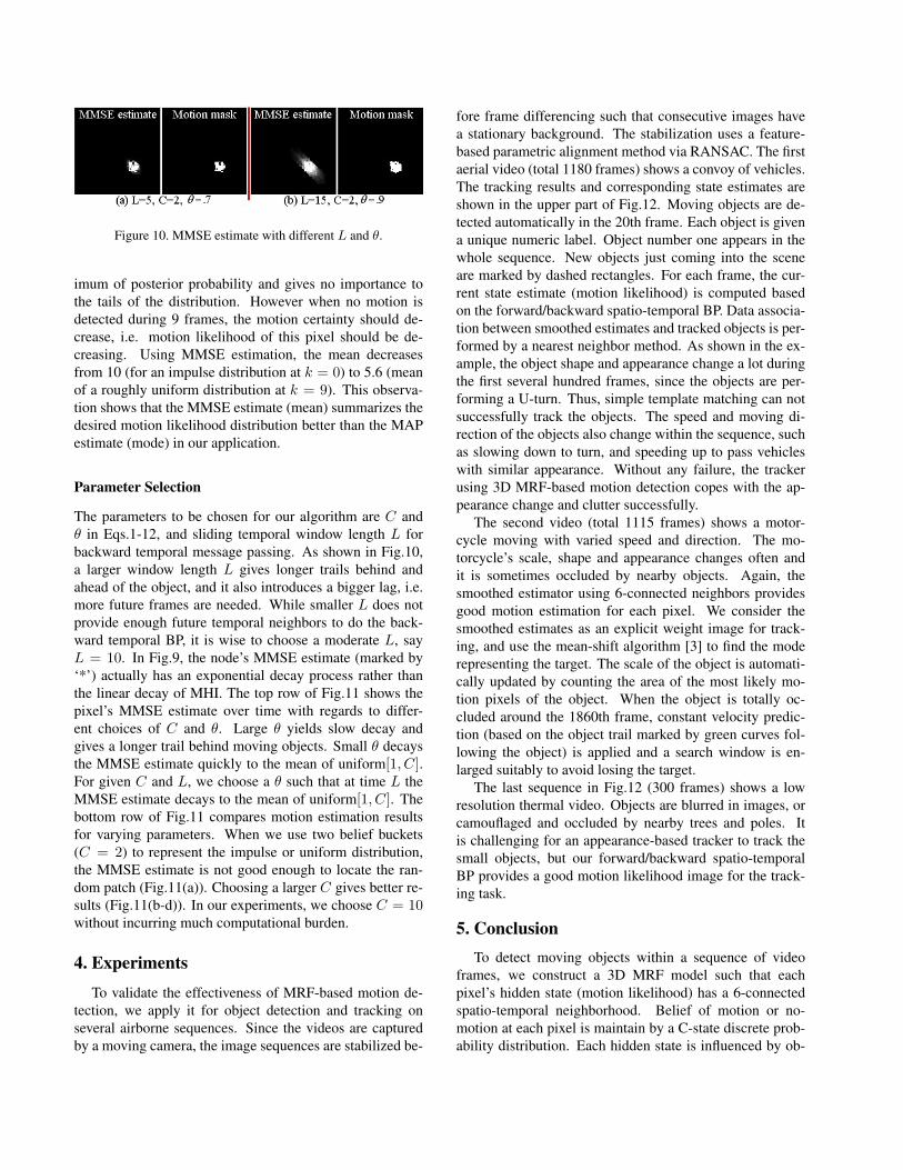
Figure 10. MMSE estimate with different L and θ.

imum of posterior probability and gives no importance tothe tails of the distribution. However when no motion isdetected during 9 frames, the motion certainty should de-crease, i.e. motion likelihood of this pixel should be de-creasing. Using MMSE estimation, the mean decreasesfrom 10 (for an impulse distribution at k = 0) to 5.6 (meanof a roughly uniform distribution at k = 9). This observa-tion shows that the MMSE estimate (mean) summarizes thedesired motion likelihood distribution better than the MAPestimate (mode) in our application.

Parameter Selection

The parameters to be chosen for our algorithm are C andθ in Eqs.1-12, and sliding temporal window length L forbackward temporal message passing. As shown in Fig.10,a larger window length L gives longer trails behind andahead of the object, and it also introduces a bigger lag, i.e.more future frames are needed. While smaller L does notprovide enough future temporal neighbors to do the back-ward temporal BP, it is wise to choose a moderate L, sayL = 10. In Fig.9, the node’s MMSE estimate (marked by‘*’) actually has an exponential decay process rather thanthe linear decay of MHI. The top row of Fig.11 shows thepixel’s MMSE estimate over time with regards to differ-ent choices of C and θ. Large θ yields slow decay andgives a longer trail behind moving objects. Small θ decaysthe MMSE estimate quickly to the mean of uniform[1, C].For given C and L, we choose a θ such that at time L theMMSE estimate decays to the mean of uniform[1, C]. Thebottom row of Fig.11 compares motion estimation resultsfor varying parameters. When we use two belief buckets(C = 2) to represent the impulse or uniform distribution,the MMSE estimate is not good enough to locate the ran-dom patch (Fig.11(a)). Choosing a larger C gives better re-sults (Fig.11(b-d)). In our experiments, we choose C = 10without incurring much computational burden.

4. Experiments

To validate the effectiveness of MRF-based motion de-tection, we apply it for object detection and tracking onseveral airborne sequences. Since the videos are capturedby a moving camera, the image sequences are stabilized be-

fore frame differencing such that consecutive images havea stationary background. The stabilization uses a feature-based parametric alignment method via RANSAC. The firstaerial video (total 1180 frames) shows a convoy of vehicles.The tracking results and corresponding state estimates areshown in the upper part of Fig.12. Moving objects are de-tected automatically in the 20th frame. Each object is givena unique numeric label. Object number one appears in thewhole sequence. New objects just coming into the sceneare marked by dashed rectangles. For each frame, the cur-rent state estimate (motion likelihood) is computed basedon the forward/backward spatio-temporal BP. Data associa-tion between smoothed estimates and tracked objects is per-formed by a nearest neighbor method. As shown in the ex-ample, the object shape and appearance change a lot duringthe first several hundred frames, since the objects are per-forming a U-turn. Thus, simple template matching can notsuccessfully track the objects. The speed and moving di-rection of the objects also change within the sequence, suchas slowing down to turn, and speeding up to pass vehicleswith similar appearance. Without any failure, the trackerusing 3D MRF-based motion detection copes with the ap-pearance change and clutter successfully.

The second video (total 1115 frames) shows a motor-cycle moving with varied speed and direction. The mo-torcycle’s scale, shape and appearance changes often andit is sometimes occluded by nearby objects. Again, thesmoothed estimator using 6-connected neighbors providesgood motion estimation for each pixel. We consider thesmoothed estimates as an explicit weight image for track-ing, and use the mean-shift algorithm [3] to find the moderepresenting the target. The scale of the object is automati-cally updated by counting the area of the most likely mo-tion pixels of the object. When the object is totally oc-cluded around the 1860th frame, constant velocity predic-tion (based on the object trail marked by green curves fol-lowing the object) is applied and a search window is en-larged suitably to avoid losing the target.

The last sequence in Fig.12 (300 frames) shows a lowresolution thermal video. Objects are blurred in images, orcamouflaged and occluded by nearby trees and poles. Itis challenging for an appearance-based tracker to track thesmall objects, but our forward/backward spatio-temporalBP provides a good motion likelihood image for the track-ing task.

5. ConclusionTo detect moving objects within a sequence of video

frames, we construct a 3D MRF model such that eachpixel’s hidden state (motion likelihood) has a 6-connectedspatio-temporal neighborhood. Belief of motion or no-motion at each pixel is maintain by a C-state discrete prob-ability distribution. Each hidden state is influenced by ob-

Figure 11. Top row: MMSE estimates of one pixel over time with respect to different θ’s and C’s; Bottom row: Comparison of MMSEestimates of all pixels and thresholded motion masks at one time instant with respect to chosen θ and C.

Figure 12. Experimental results on three video sequences.

served inter-frame difference data such that an observed in-tensity difference at a pixel introduces an impulse spike atstate C of the motion likelihood, whereas no observed inten-sity difference results in a uniform distribution across like-lihood states. A compatibility function on spatio-temporalcliques is defined via the Potts model, which in the absenceof observed intensity differences at a pixel serves to decaymotion belief towards a uniform distribution (representingno-motion). Within the 2D spatial grid graph, asynchronousaccelerated message updating is performed on all pixelsfor each frame, and along the temporal axis, 1D BP (for-ward/backward) is applied on each pixel through time. Thuseach pixel’s hidden state node incorporates its six neigh-bor’s messages to decide its state. The MMSE estimate ofthe state at each node provides an accurate and smooth esti-mate of the pixel’s motion likelihood.

In this paper, the 3D MRF-based detector deals well withdifficult motion detection and tracking problems such as ob-jects with uniform color and objects camouflaged by similarappearance to the background. The approach is validated onseveral synthesized and real-world video sequences. So far,only motion information is smoothed to estimate the currentstate. In future work, other cues such as shape and appear-ance can be fused into the 3D MRF network and processedby Belief Propagation.

AcknowledgmentsThis work was funded under the NSF Computer Vision

program via grant IIS-0535324 on Persistent Tracking.

References[1] A. Bobick and J. Davis, “The Recognition of Human Move-

ment Using Temporal Templates,” IEEE Transactions Pat-tern Analysis and Machine Intelligence, 23(3): p257-267March 2001.

[2] R. Collins, A. Lipton, H. Fujiyoshi and T. Kanade, “Al-gorithms for Cooperative Multi-Sensor Surveillance,” Pro-ceedings of the IEEE, 89(10): p1456-1477, October 2001.

[3] D. Comaniciu, V. Ramesh and P. Meer, “Kernel-Based Ob-ject Tracking,” IEEE Transactions Pattern Analysis and Ma-chine Intelligence, 25(5): 564-577 May 2003.

[4] P. Felzenszwalb and D. Huttenlocher, “Efficient belief prop-agation for early vision,” In IEEE Conference on ComputerVision and Pattern Recognition, p261-268, 2004.

[5] C. Fox and G. Nicholls, “Exact map states and expectationsfrom perfect sampling: Greig, Porteous and Seheult revis-ited,” In Proc. Twentieth Int. Workshop on Bayesian Infer-ence and Maximum Entropy Methods in Sci. and Eng., 2000

[6] W. Freeman, E. Pasztor and O. Carmichael, “Learning Low-Level Vision,” International Journal of Computer Vision,40(1): p25-47, 2000.

[7] I. Haritaoglu, D. Harwood and L. Davis, “W4: Real-timeSurveillance of People and Their Activities,” IEEE Trans-actions Pattern Analysis and Machine Intelligence, 22(8):p809-830 August 2000.

[8] M. Irani and P. Anandan, “A Unified Approach to MovingObject Detection in 2D and 3D Scenes,” IEEE TransactionsPattern Analysis and Machine Intelligence, 20(6): p577-589June 1998.

[9] M. Isard and A. Blake. “A smoothing filter for Condensa-tion.” In Proceedings of the 5th European Conference onComputer Vision, p767-781, 1998.

[10] R. Kumar, H. Sawhney et.al, “Aerial Video Surveillance andExploitation,” In Proceedings of the IEEE, 89(10): p1518-1539 October 2001.

[11] X. Lan, S. Roth et.al, “Efficient Belief Propagation withLearned Higher-Order Markov Random Fields.” In Proceed-ings of the 9th European Conference on Computer Vision,p269-282, 2006.

[12] F. Luthon, A. Caplier and M. Lievin, “Spatiotemporal MRFapproach to video segmentation: application to motion de-tection and lip segmentation.” Signal Processing, 76(1):p61-80, July 1999.

[13] R. Szeliski, R. Zabih et.al, “A Comparative Study of En-ergy Minimization Methods for Markov Random Fields.” InProceedings of the 9th European Conference on ComputerVision, p19-26, 2006.

[14] M. Tappen and W. Freeman, “Comparison of graph cuts withbelief propagation for stereo, using identical MRF parame-ters.” In: ICCV, p900-907, 2003

[15] L. Wixson, “Detecting Salient Motion by AccumulatingDirectionally-Consistent Flow, ” IEEE Transactions PatternAnalysis and Machine Intelligence, 22(8): p774-780 August2000.

[16] J. Yedidia, W. Freeman and Y. Weiss, “Generalized beliefpropagation.” In: NIPS, p689-695, 2000