Bayesian Evaluation and Selection Strategies in PortfolioDecision Analysis

Eeva Vilkkumaa∗, Juuso Liesiö, Ahti SaloDepartment of Mathematics and Systems Analysis, School of Science, Aalto University, P.O.

Box 11100, 00076 Aalto, Finland

Abstract

Practically all firms pursue goals by selecting a portfolio of courses of action thatconsume resources. Yet, due to uncertainties such as unforeseen market develop-ments, it may not be possible to know in advance how much value these actionsyield. Thus, the selection must be based on uncertain ex ante estimates aboutthe future values of the actions. In this paper we show that the explicit Bayesianmodeling of these uncertainties serves to increase both the expected value of theselected portfolio and the expected number of those selected actions that belongto the ex post optimal portfolio. Bayesian modeling is also shown to eliminatethe expected negative gap between the true and estimated portfolio value, whichis caused not by biased value estimates but by the statistical properties of opti-mizing under uncertainty. Furthermore, we offer analytic results for the optimaltargeting of additional evaluations and show that it often suffices to re-evaluateonly a subset of the actions. Finally, we propose a novel project performancemeasure, which is the probability that the project belongs to the optimal portfo-lio.Keywords: Decision analysis, Portfolio selection, Bayesian methods, Value ofinformation

∗Corresponding author. Tel.: +358 9 470 25885; Fax: +358 9 470 23096,Email addresses: eeva.vilkkumaa@aalto.fi (Eeva Vilkkumaa),

juuso.liesio@aalto.fi (Juuso Liesiö), ahti.salo@aalto.fi (Ahti Salo)

Preprint submitted to European Journal of Operational Research September 12, 2012

1. Introduction

Allocating resources among alternative courses of action is a recurring activityin most organizations (Salo, Keisler, and Morton, 2011). Industrial firms, forinstance, start research and development projects based on expectations aboutthe projects’ future revenues. Municipalities allocate public funds to facilities thatdeliver social and educational services to their citizens. While these problems areseemingly different, they are methodologically similar in that there is a portfolioof actions (referred to as projects in the rest of the paper) which is to be selectedsubject to the availability of scarce resources.

More formally, projects are typically selected based on ex ante evaluationsabout their future value. Depending on the problem context, this value maybe measured in terms of the net present value (NPV), the benefit-to-cost ratio(BCR) or a multicriteria value function, for instance. The evaluations are usuallyuncertain due to reasons such as future market developments or unforeseeableinnovations. These uncertainties make it difficult to determine the optimal selec-tions (i.e., projects that belong to the ex post optimal portfolio), and hence theresulting portfolio is likely to be suboptimal. Furthermore, it can be shown thateven if the estimates for the projects’ values are unbiased, the value of the se-lected portfolio is systematically overestimated, causing the decision-maker (DM)to experience post-decision disappointment (Brown, 1974; Harrison and March,1984; Smith and Winkler, 2006).

In this paper, we show that the explicit Bayesian modeling of evaluation un-certainties (i) increases the expected portfolio value, (ii) raises the expected num-ber of optimal selections and (iii) alleviates post-decision disappointment. TheBayesian framework also allows us to study analytically the extent to which theacquisition of additional project evaluations increases expected portfolio value.In particular, we show that additional evaluations should be targeted on thoseprojects that (i) have initial value estimates close to the selection threshold, (ii)can be re-evaluated relatively accurately, and (iii) are uncertain in the sense thatthe distribution of their initial value estimates has a relatively high variance. Oursimulation experiments suggest that, in keeping with these guidelines, it sufficesto re-evaluate only a fraction of the projects to gain almost as much additionalvalue as by conducting a complete re-evaluation. Because the evaluation pro-

2

cess can be expensive and time consuming, this result is of considerable practicalrelevance.

The rest of the paper is structured as follows. In Section 2 we briefly dis-cuss earlier research on uncertainty modeling in project portfolio selection. InSection 3 we present our framework and illustrate the issued due the estima-tion uncertainties. The explicit modeling of these uncertainties through Bayesianmethods is studied in Section 4. In Section 5 we discuss the practical implicationsof our results. Section 6 concludes.

2. Earlier Approaches to Modelling Uncertainty

Methods of portfolio decision analysis are widely employed to support projectportfolio selection in a variety of contexts in both public administration (e.g. Go-labi, Kirkwood, and Sicherman, 1981; Kleinmuntz and Kleinmuntz, 1999) andindustrial organizations (e.g. Stummer and Heidenberger, 2003; Liesiö, Mild, andSalo, 2008). In particular, different approaches have been developed to captureuncertainties about the projects’ values. For instance, methods that use set in-clusion of feasible parameters have been applied in decision contexts such as theselection of road pavement projects (Liesiö, Mild, and Salo, 2007), developmentof strategic plans for air traffic management (Grushka-Cockayne, De Reyck, andDegraeve, 2008), the selection of a strategic product portfolio in a telecommu-nications company (Lindstedt, Liesiö, and Salo, 2008) and scenario-based fore-sight (Liesiö and Salo, 2012).

In project selection, Bayesian modeling of uncertainties means that the priorbelief about a project’s future value is updated in view of ex ante evaluationinformation. Analogous techniques have a long tradition in financial portfolioselection, where Bayesian analysis is used to both revise the model parametersand to predict security prices with the aim of optimally allocating the currentwealth among the securities (Winkler and Barry, 1975; Barry and Winkler, 1976;Aguilar and West, 2000; Polson and Tew, 2000; Brandt et al., 2005; Soyer andTanyeri, 2006). However, financial portfolio selection differs from project port-folio selection in several respects. First, a project has no market price; rather,its estimated value is typically derived from expert opinions about relevant con-cerns, such as the project’s societal and environmental impact. Second, a project

3

can either be selected or not so that the decision variables are binary, whereasin financial portfolio selection, it is possible to allocate any fractional amountof the budget to a security. Finally, whereas security prices are often heavilycorrelated, project interdependencies stem mainly from the constraint structureof the problem including, for instance, mutual exclusiveness (either project A orproject B can be selected but not both) or logical constraints (project B can onlybe selected if A is selected).

Beyond finance, it has been noted that in prediction tasks, people typicallyneglect the prior information or the ‘base rate’ of the outcome. Instead, peoplemake judgments based merely on the evidence at hand, leading them to erro-neously predict rare events and extreme values (Kahneman and Tversky, 1973,1979). When selecting a single best alternative out of many, this means that theestimated value of the recommended alternative is likely to be overly optimistic,causing the DM to experience post-decision disappointment once the true valueis realized. Bayesian adjustment of uncertain value estimates has been shownto eliminate the post-decision disappointment, i.e., the expected negative gapbetween the true and estimated value of the selected alternative (Brown, 1974;Harrison and March, 1984; Smith and Winkler, 2006).

Harrison and March (1984) recognize the practical difficulties of assessing theBayesian adjustment parameters in an arbitrary decision context. They arguethat reducing estimation uncertainties tends to increase the value of the selectedalternative and to decrease the level of post-decision disappointment. This recog-nition has motivated research on the value of information and its dependence onthe parameters of the decision problem. Yet, many studies conclude that thevalue of information varies in unexpected, ambiguous and sometimes counterin-tuitive ways (Gould, 1974; Laffont, 1976; Hilton, 1981; Eeckhoudt and Godfroid,2000). Delquié (2008), however, shows that under very general assumptions, thevalue of information in choosing between two alternatives is highest when the DMis initially indifferent between the two, and that the value is lower when the initialpreference for one of the alternatives is stronger. Bickel (2008) obtain a similarresult for the value of imperfect information relative to perfect information in adecision problem with normal priors and exponential utility.

Frazier and Powell (2010) study optimal information collection for selecting

4

a single best alternative out of many, when both the prior and the sampling dis-tribution are normal. They find that with many a priori identical alternatives,it pays off to obtain additional information about only a subset of the alterna-tives such that this subset becomes smaller when estimation accuracy improves.Furthermore, they investigate the concavity characteristics of the marginal valueof information and develop a fully sequential information collection strategy thathelps overcome the challenge of potential non-concavity of the marginal value.

In the context of portfolio decision analysis, the value of information has beenstudied mostly through simulation studies. Keisler (2004), for instance, simulatesdifferent portfolio selection strategies and demonstrates that the value added bythe systematic prioritization of project proposals (compared to random funding)often exceeds the value added through the development of very accurate estimatesof the projects’ values. In Keisler (2009), he uses a similar approach to study thevalue of assessing weights in multicriteria portfolio decision analysis.

3. Project Portfolio Selection under Uncertainty

Consider a set of project proposals i = 1, . . . ,m which, if funded, will yieldvalues v = [v1, . . . , vm]

′. These so-called ‘true values’ v are realizations of randomvariables V = [V1, . . . , Vm]

′ ∼ f(v) such that the joint distribution function f(v)

is assumed to be known.1 The term ‘true value’ here refers to the ex post realizedvalue of the project, observed possibly long after the project has been completed;see e.g. Arnott, Li, and Sherrerd (2009).

The DM wants to select a portfolio of projects such that the sum of theselected projects’ true values is maximized. The selection decision is denotedby z = [z1, . . . zm] such that z is a binary row vector with zi = 1 if and only ifproject i is selected. The selection is subject to resource and other constraintsthat define the set of feasible portfolios Z. If the true values v were known, the

1Throughout this paper random variables are denoted by capital letters, and their fixedrealizations by the lower-case counterparts.

5

optimal portfolio z(v) could be determined from the optimization problem2

z(v) = argmaxz∈Z

zv. (1)

In reality, the DM does not know the true values v, but only estimatesvE = [vE1 , . . . , v

Em]

′ of v. These estimates are assumed to be a realizationof a random variable (V E|V ) ∼ f(vE|v) with a known distribution functionf(vE|v) such that the estimates are conditionally unbiased, i.e., E[V E

i |V = v] =∫∞−∞ vEi f(v

Ei |v)dvEi = vi. After observing the estimates vE, the DM selects the

portfolio z(vE) by solving the optimization problem

z(vE) = argmaxz∈Z

zvE. (2)

Using the value estimates vE only without accounting for the implicationsof estimation uncertainties in the selection problem can be problematic. Forexample, consider the selection of a portfolio of projects A, . . . , J , whose costs varyin the range from 1 to 12 Me . The budget is 25 Me. Here, the projects’ valuesvi are realizations of independent and identically distributed random variablesVi = µi +Ei, where µi = 10 and Ei ∼ N(0, 32), i = A, . . . , J . Projects A throughD are conventional projects, whose future performance can be estimated relativelyaccurately; this is modeled so that (V E

i |Vi = vi) = vi +∆i with ∆i ∼ N(0, 12) fori = A, . . . , D. Projects E through J , on the other hand, are novel, radical projectsabout which it is much more difficult to obtain reliable estimation information;(V E

i |Vi = vi) = vi + ∆i with ∆i ∼ N(0, 2.82) for i = E, . . . , J . Project B isa follow-up project for A, and thus can be selected only on condition that A isselected.

Figure 1 illustrates one possible realization of this decision setting. The size ofthe markers is proportional to the project cost. If the projects’ true values wereknown in advance, the DM would select projects {C,D,G, I, J}. In reality, onlythe estimates are observed, so that projects {C,D,E,H, J} marked with blackcircles are selected.

Based on this example, we highlight three concerns that are typically encoun-tered in portfolio selection under uncertainty:

2If there are multiple solutions to the maximization problem, z(·) is selected at randomamong these solutions.

6

0 2 4 6 8 10 12 14 16 180

2

4

6

8

10

12

14

16

18

True value v (MEUR)

Est

imat

ed v

alue

vE (

ME

UR

)

A

B

C

D

E

F

G

H

I

J * *

*

*

*

Figure 1: The true and estimated values of 10 projects, marker size proportional to projectcost. B can only be selected if A is selected. Vi = 10 +Ei, Ei ∼ N(0, 32) ∀i. For i = A, . . . ,D:(V E

i |Vi = vi) = vi +∆i, ∆i ∼ N(0, 12). For i = E, . . . , J : ∆i ∼ N(0, 2.82). The truly optimalportfolio z(v) = {C,D,G, I, J} (asterisks); the recommended portfolio z(vE) = {C,D,E,H, J}(black markers).

(i) Suboptimal portfolio value: The true value of the selected portfolio (51.6Me) is 7% lower than that of the optimal portfolio (55.3 Me).

(ii) Non-optimal selections: The ‘radical’ projects E and H that do notbelong to the truly optimal portfolio have been selected as a result of over-estimation.

(iii) Post-decision disappointment: The ex ante value estimate of the se-lected portfolio (62.1 Me) is 21% higher than its true value ex post (51.6Me).

Although Figure 1 presents a single realization of a portfolio selection problem,the above concerns apply even when averaged over a large number of selection

7

processes. More specifically, by consistently selecting portfolios based on uncer-tain estimates, the DM will not maximize the expected portfolio value; nor willshe maximize the expected number of projects that belong to the optimal portfo-lio. Furthermore, the true value of the selected portfolio will, on average, be lowerthan estimated. The logic behind this phenomenon is, in short, that the morethe value of a project has been overestimated, the more probable it is that thisproject will be selected. Thus, even if the value estimates are unbiased a priori,the optimization-based selection process implies that the estimates for the recom-mended projects in (2) tend to have an upward bias. The general phenomenon isformalized in Proposition 1, which does not make specific assumptions about thedistributions f(v) and f(vE|v) or about the feasibility constraints. All proofs arein the Appendix.

Proposition 1. Let V E be a conditionally unbiased estimator of V . Then,

E[z(V E)V − z(V E)V E] ≤ 0,

where z(V E) is obtained from (2). Moreover, if P(z(V ) ̸= z(V E)) > 0, wherez(V ) is obtained from (1), then E[z(V E)V − z(V E)V E] < 0.

Proposition 1 states that, on average, the selected portfolio z(vE) will not yieldmore than its estimated value. Furthermore, if there is a positive probabilityof selecting ‘wrong’ projects – as there always is, whenever the estimates maydiffer from the true values – the expected gap between the true and estimatedportfolio value is strictly negative. This means that even if the value estimates areunbiased, the portfolio value will be systematically overestimated when averagedover a large number of selection processes. Thus, the DM will experience post-decision disappointment.

The more uncertain the value estimates, the larger the disappointment – in-deed, a large variance in estimation errors not only makes it more difficult toidentify the best projects, but also implies that the values of the selected projectsare likely to have been significantly overestimated. Figure 2 illustrates the effectof estimation uncertainties on the magnitude of post-decision disappointment.In this Figure, the selection of 10 projects out of 100 with true values vi drawnfrom the standard normal distribution has been simulated with different levels of

8

standard deviation τ of the additive, normally distributed zero-mean estimationerror. For instance, when τ = 0.8, the average estimated value of the selectedportfolio is 22.16, which is 65% higher than the expected true value 13.45.

0 0.2 0.4 0.6 0.8 112

14

16

18

20

22

24

26

Standard deviation of estimation error

Por

tfolio

val

ue

EstimatedTrue

PDD

Figure 2: The average true (solid) and estimated (dashed) values of the selected portfolioas functions of the standard deviation of the normally distributed zero-mean estimation error.Selection of 10 out of 100 projects with true values drawn from the standard normal distribution.1000 simulation rounds (Monte Carlo).

4. Bayesian Modeling of Uncertainty in Portfolio Selection

Because the DM does not know the projects’ true values a priori, the prob-lems of suboptimal portfolio value, non-optimal selections and post-decision dis-appointment cannot be fully avoided. Nevertheless, they can be alleviated byexplicitly modeling the underlying uncertainties through Bayesian methods (foran overview, see e.g. Gelman et al. 2004). That is, assuming that the prior dis-tribution f(v) for the true values and the likelihood distribution f(vE|v) for theestimates are known, the posterior distribution f(v|vE) for the true values giventhe estimates can be obtained by using Bayes’ rule f(v|vE) ∝ f(v)f(vE|v). Withthe help of the posterior distribution, it is possible to study notions such as the

9

expected true value E[Vi|V E = vE] of project i given the estimates, or the prob-ability P(zi(V ) = 1|V E = vE) of project i being included in the truly optimalportfolio. These notions can then be used to formulate optimization problems forportfolio selection with the aim of either (i) maximizing the expected portfoliovalue or (ii) maximizing the expected number of optimal selections. Furthermore,the posterior distribution allows us to study the value of information in portfo-lio selection. This leads us to formulate guidelines for the applying cost-efficientproject re-evaluation strategies.

4.1. Maximization of the Expected Portfolio Value

When maximizing the expected portfolio value, the objective function iszE[V |V E = vE]. Thus, project selection is based on the Bayes estimatesvB = [vB1 . . . , vBm]

′, which are computed from the observed estimates vE through

vBi = E[Vi|V E = vE] =

∫ ∞

−∞vif(vi|vE)dvi. (3)

The Bayes estimate for project i is thus the mean of the posterior distributionf(vi|vE). The portfolio that maximizes the expected value is determined by

z(vB) = argmaxz∈Z

zE[V |V E = vE] = argmaxz∈Z

zvB. (4)

To study the average performance of selection rule (4) we need to define the Bayesestimator V B = [V B

1 , . . . , V Bm ]′ (a random variable), which is obtained from (3)

by replacing the observed estimates vE with the random variable V E:

V Bi = E[Vi|V E] =

∫ ∞

−∞vif(vi|V E)dvi. (5)

Under very general assumptions, the selection based on the Bayes estimates canbe expected to yield at least as much value as the portfolio which maximizes thesum of the initial value estimates vE.

Proposition 2. Let V E, V , and z(V E) be as in Proposition 1. Then,

E[z(V E)V − z(V B)V ] ≤ 0,

where V B is given by (5) and z(V B) is obtained from (4). Moreover, if P(z(V E) ̸=z(V B)) > 0, then E[z(V E)V − z(V B)V ] < 0.

10

This is an intuitive result because by (4), z(vB) maximizes the expected portfoliovalue. Nevertheless, if there is a positive probability of selecting a different port-folio when using Bayes estimates than by using the estimates as such, the averagevalue of the selected portfolio is strictly better. Generally P(z(V E) ̸= z(V B)) > 0,implying that Bayes estimates do yield a higher expected portfolio value.

A closed form expression for the Bayes estimate can be provided if the projects’values and the value estimates are generated by conjugate distributions. Forexample, assume that both the true values and the estimation errors follow theself-conjugate normal distribution so that for each project i

True values: Vi = µi + Ei, Ei ∼ N(0, σ2i ),

Estimates: (V Ei |Vi = vi) = vi +∆i, ∆i ∼ N(0, τ 2i ).

Then, the Bayes estimate in (3) becomes

vBi = αivEi + (1− αi)µi, where αi =

(1 +

τ 2iσ2i

)−1

. (6)

For the normal distribution, the Bayes estimate is thus a weighted averageof the prior mean and the observed estimate. The weighting is determined bythe variance ratio τ 2i /σ

2i . If the estimate is very uncertain so that the estimation

error variance τ 2i is very large compared to the prior variance σ2i , it follows that

the weight αi of the estimate vEi is small and more emphasis is given to priorexpectation µi. On the other hand, with very accurate estimates and/or verylarge prior variance, αi approaches 1. This means that the estimate offers highlyreliable information about the project’s true value.

If the prior distribution of values f(v) and the likelihood distribution f(vE|v)are not conjugate, the Bayes estimates can be computed through numerical inte-gration or simulation. Essentially, this requires the approximation of the posteriordistribution f(vi|vE) for each project i. This can be done, for instance, by form-ing a discrete joint distribution for Vi and V E by first sampling L values of vi(ℓ),ℓ = 1, . . . , L from the prior and then, corresponding to each vi(ℓ), K vectorsof vE(ℓ, k), k = 1, . . . , K from the conditional distribution for (V E|Vi = vi(ℓ)).The posterior distribution corresponding to the initial estimates vE can then befound by setting V E = vE in the discrete joint distribution and by normalizingthe resulting marginal distribution function.

11

If the discretization is dense enough, the above method works well for problemswith independent project values. There are indeed many decision contexts inwhich the projects’ values are essentially independent; for instance, in the fundingof public research projects, the value of a project proposal usually does not dependon that of the others. However, if there are dependencies among the projects’values and value estimates, sampling a sufficient amount of data at every pointin a dense multi-dimensional grid may become prohibitively expensive. Moreefficient simulation and numerical integration strategies for such cases have beendeveloped by, e.g., Müller (1999) and Gelman et al. (2004).

4.2. Mitigation of Post-Decision Disappointment

The Bayes estimates shift expectations from the estimates towards prior valueinformation f(v); and, more specifically, towards the prior mean µi, if the truevalues and estimation errors are normally distributed. Thus, they could be ex-pected to yield more conservative (i.e., less overestimated) assessments about thevalue of the selected portfolio. It turns out, that without specific assumptionsabout the distributions f(v) and f(vE|v) or about the problem constraints, Bayesestimates eliminate the expected gap between the true and estimated value of theselected portfolio.

Proposition 3. Let V , V E, V B, and z(·) be as in Proposition 2. Then

E[z(vB)V − z(vB)vB|V E = vE] = 0

for all vE, and hence E[z(V B)V − z(V B)V B] = 0.

Proposition 3 states that the expected difference between the ex post truevalue of the selected portfolio and its value determined by the Bayes estimates iszero. Nevertheless, even in individual cases the Bayes estimates serve to alleviatepost-decision disappointment, because extreme Bayes estimates vBi are less prob-able than extreme estimates vEi . Figure 3 illustrates the Bayesian adjustment ofuncertain value estimates using the same data as in Figure 1. Based on the Bayesestimates in Figure 3(b), portfolio {A,B,C,D, I, J} is selected.

Compared to the estimates in Figure 3(a), the Bayes estimates in Figure 3(b)are closer to the common prior mean 10, especially for projects E through J with

12

a high estimation error variance: for instance, the Bayes estimate of project H

with initial estimate vEH = 16.56 is

vBH =(1 +

2.82

32

)−1

· 16.56 +

(1−

(1 +

2.82

32

)−1)

· 10 = 13.96.

Due to the Bayesian adjustment, the degree of overestimation of project H andunderestimation of project I is much lower. Based on the initial estimates vE,the value of the selected portfolio is overestimated by 21%; by using the Bayesestimates vB, on the other hand, the estimated value of the selected portfoliois only 7% higher than the true value. Furthermore, the true value of portfolioz(vB) is only 1% lower than optimal.

0 2 4 6 8 10 12 14 16 180

2

4

6

8

10

12

14

16

18

True value v (MEUR)

Est

imat

e vE

(M

EU

R)

AB

C

D

E

F

G

H

I

JPrior mean

**

*

*

*

(a) True values vs. estimates

0 2 4 6 8 10 12 14 16 180

2

4

6

8

10

12

14

16

18

1

True value v (MEUR)

Bay

es e

stim

ate

vB (

ME

UR

)

A

F

I

E

J

B

D C

H

G

Prior mean

*

* ** *

*

(b) True values vs. Bayes estimates

Figure 3: True values, estimates and Bayes estimates of 10 projects, marker size proportionalto project cost. A can only be selected if B is selected. Vi = 10 + Ei, Ei ∼ N(0, 32) ∀i. Fori = A, . . . ,D, estimation error ∆i ∼ N(0, 12); for i = E, . . . , J , estimation error ∆i ∼ N(0, 2.82).The truly optimal portfolio z(v) is marked with asterisks, z(vE) with black markers in Figure(a), and z(vB) with black markers Figure (b).

4.3. Maximization of the Expected Number of Optimal Selections

The Bayesian approach can be used to analyze the number of selected projectsthat can be expected to belong to the optimal portfolio. This can be particu-larly relevant in contexts where the projects’ values are not estimated with awell-defined measure such as the NPV. In public research project funding, forinstance, the value estimates are typically expert opinions that reflect several

13

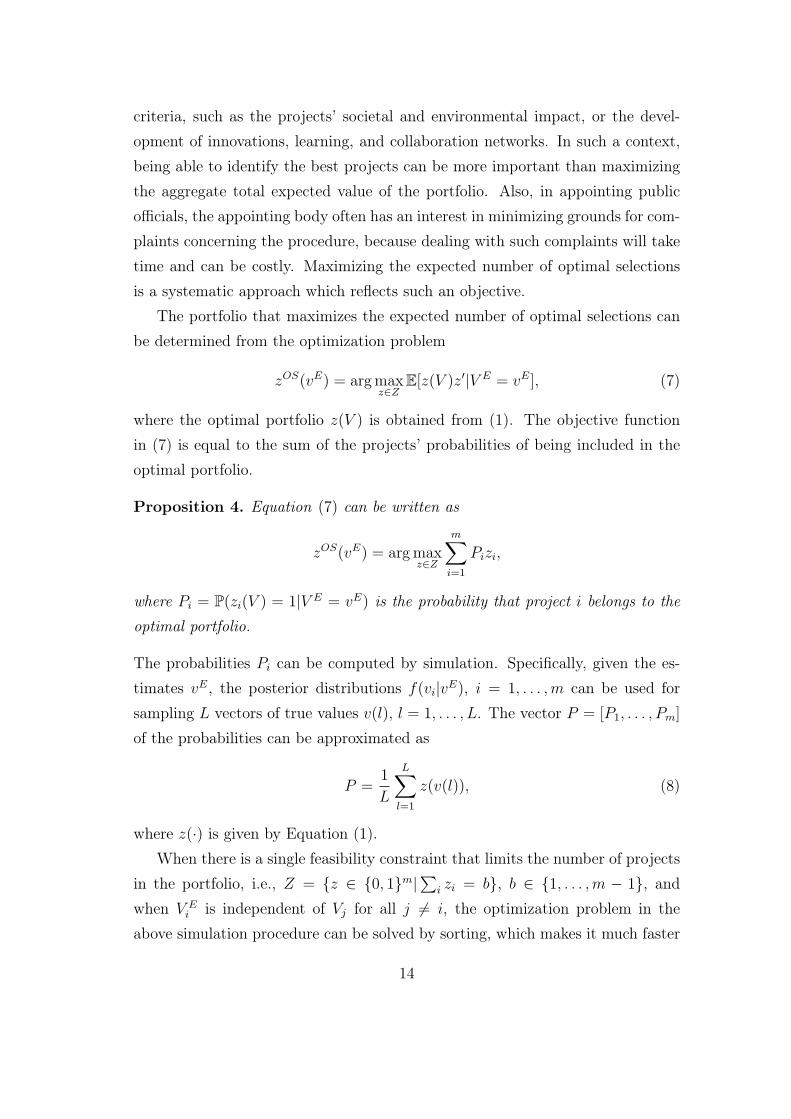
criteria, such as the projects’ societal and environmental impact, or the devel-opment of innovations, learning, and collaboration networks. In such a context,being able to identify the best projects can be more important than maximizingthe aggregate total expected value of the portfolio. Also, in appointing publicofficials, the appointing body often has an interest in minimizing grounds for com-plaints concerning the procedure, because dealing with such complaints will taketime and can be costly. Maximizing the expected number of optimal selectionsis a systematic approach which reflects such an objective.

The portfolio that maximizes the expected number of optimal selections canbe determined from the optimization problem

zOS(vE) = argmaxz∈Z

E[z(V )z′|V E = vE], (7)

where the optimal portfolio z(V ) is obtained from (1). The objective functionin (7) is equal to the sum of the projects’ probabilities of being included in theoptimal portfolio.

Proposition 4. Equation (7) can be written as

zOS(vE) = argmaxz∈Z

m∑i=1

Pizi,

where Pi = P(zi(V ) = 1|V E = vE) is the probability that project i belongs to theoptimal portfolio.

The probabilities Pi can be computed by simulation. Specifically, given the es-timates vE, the posterior distributions f(vi|vE), i = 1, . . . ,m can be used forsampling L vectors of true values v(l), l = 1, . . . , L. The vector P = [P1, . . . , Pm]

of the probabilities can be approximated as

P =1

L

L∑l=1

z(v(l)), (8)

where z(·) is given by Equation (1).When there is a single feasibility constraint that limits the number of projects

in the portfolio, i.e., Z = {z ∈ {0, 1}m|∑

i zi = b}, b ∈ {1, . . . ,m − 1}, andwhen V E

i is independent of Vj for all j ̸= i, the optimization problem in theabove simulation procedure can be solved by sorting, which makes it much faster

14

to compute Pi. Moreover, Pi can be computed exactly (apart from errors innumerical integration) in polynomial time. Denoting Ji = {1, . . . ,m} \ {i}, wehave

Pi =

∫ ∞

−∞f(vi|vE)

∑J ′⊆Ji|J ′|<b

∏j∈J ′

P(Vj > vi|V E = vE)∏

j∈Ji\J ′

P(Vj < vi|V E = vE)dvi.

(9)The computational effort of evaluating (9) is proportional to Lm2, where L is thenumber of points at which the integrand is evaluated (Chen and Jun, 1997).

Table 1 shows the Pi-measures using the same data as in Figures 1 and 3. Thebolded numbers in each column of Table 1 indicate which projects are selected.Here z(vB) = zOS(vE); however, the Bayes estimates and the Pi-measures do notin general result in the same portfolio. In fact, the expected value of portfoliozOS(vE) may in some cases be far from optimal. Moreover, the available resourcesmay not be efficiently utilized.

For example, assume that there are five projects A, . . . , E such that projectsA and B consume one resource unit and projects C, D, E four resource unitseach. The budget is five resource units. The Bayesian estimated benefit-to-costratio (BCR; value divided by cost) is the same for each project. Moreover, theprior distribution of the BCR and the conditional distribution of the estimatedBCR are the same for all projects. All truly optimal portfolios are thus expectedto contain one project from set {A,B} and one from set {C,D,E} so that thereare six alternative portfolios which are optimal with equal probability. Hence,we have PA = PB = 1/2 and PC = PD = PE = 1/3. If the expected numberof optimal selections is maximized, projects A and B are selected, which wouldyield 60% lower expected portfolio value and leave three resource units unused.

The Pi-measures are nevertheless useful in analyzing individual projects evenif the primary objective is the maximization of the expected portfolio value. Thisis because Pi describes the performance of the project not only in terms of its valueor cost, but with respect to the entire portfolio. That is, apart from reflectingthe reliability of the estimation information, Pi takes into account factors such asthe project’s cost relative to the budget or interdependencies with other projects.

Using the example of Table 1, Figure 4 illustrates the Bayes estimates vBi

so that their respective standard deviations ρi are plotted against project costs.

15

Project i vi vEi vBi Pi Cost

A 5.36 6.08 7.63 0.56 9B 10.20 9.02 9.41 0.56 3C 12.73 13.03 11.82 0.99 4D 11.07 11.11 10.67 0.70 6E 7.22 10.23 10.14 0.68 5F 4.09 4.00 6.38 0.14 7G 16.23 12.03 11.23 0.02 12H 13.44 16.56 13.96 0.30 8I 8.18 6.16 7.68 0.75 2J 7.09 11.19 10.72 0.98 1

Estimated value - 62.12 57.93 -True value 55.30 51.55 54.63 54.63

# Optimal selections (estimated) - 3.65 4.54 4.54# Optimal selections (true) 5 3 4 4

Cost 25 24 25 25

Table 1: Numerical data for 10 projects. True values vi generated from Vi ∼ N(10, 32), estimatesfrom (V E

i |Vi = vi) = vi +∆i; ∆i ∼ N(0, 12) for i = A, . . . ,D, ∆i ∼ N(0, 2.82) for i = E, . . . , J .Project B can only be selected if A is selected. Budget 25 Me.

The benefit-to-cost ratios of projects D and H are the same (1.75). The factthat H would consume one third of the budget by itself, however, is reflected inthe projects’ Pi-measures: PD = 0.7 and PH = 0.3. Furthermore, project A isclearly inferior to project H because it is both less valuable and more expensive;nevertheless, selecting project A is a necessary precondition for selecting theinexpensive project B with a high benefit-to-cost ratio (3.13), whereby A has ahigher Pi-measure (0.56) than H (0.3).

4.4. Value of Additional Evaluations

In many decision contexts, uncertainties can be reduced by obtaining addi-tional evaluations. The evaluation process may be expensive and time-consuming,and thus the DM should only re-evaluate those projects about which the addi-tional information can be expected to lead to a higher portfolio value that offsetsthe cost of the re-evaluation. In keeping with the standard definition, we treat

16

0 2 4 6 8 10 12 140

2

4

6

8

10

12

14

16

18

0.98

0.75

0.56

0.990.7

0.56

0.68

0.14

0.3

0.02

Project cost (MEUR)

Bay

es e

stim

ate

(ME

UR

)

J

I

B

C

DE

H

FA

G

BCR

Figure 4: Bayes estimates vBi ± ρi plotted against project costs using data from Table 1. Pi-measures on top. Selected projects marked with black circles.

the value of information as the increase in expected value that results from actingin accordance to the information (La Valle, 1968; Marschak and Radner, 1972;Gould, 1974; Laffont, 1980; Delquié, 2008). That is, the additional information isused to update the expected project values, based on which a different portfoliomay be recommended.

Definition 1. The expected value of information V E is

EVI[V E] = E[maxz∈Z

zE[V |V E]]−max

z∈ZzE[V ].

The definition is applicable in situations where the DM has already carried outone or more project evaluation rounds and seeks to assess the value of additionalevaluations; in this case E[V ] denotes the expected project values given the ob-served evaluations, and E[V |V E] is a random variable representing the expectedproject values after the additional evaluation V E.

Evaluating EVI in its general form is a stochastic optimization problem withbinary decision variables. In practice this means that EVI is computed through

17

simulation by sampling values of vE, using the posterior distribution to obtainE[V |V E = vE], and solving the optimization problem maxz∈Z zE[V |V E = vE] ineach simulation round. Figure 5 illustrates the EVI computed in this manner forthe example data in Figure 4, when an additional evaluation is acquired only fora single project at a time.

A comparison of Figures 5 and 4 shows that the EVI is low for projects C

and J whose Pi-measures are close to 1, and also for project G whose Pi-measureis close to 0. This makes sense: if a project is optimal/non-optimal with ahigh probability, additional information is of little use. Re-evaluating project E

with the highest benefit-to-cost ratio among the currently rejected projects yieldsan expected increase of ca. 214 ke in portfolio value, because there is a goodchance that the additional estimate will take E to the new optimal portfolio. Theinterdependent projects A and B in the currently optimal portfolio also have ahigh EVI, because A is expensive and has the lowest current estimate among theselected projects. Based on the additional estimates, either A or B may not bevaluable enough for both of them to be selected, whereby almost one half of thebudget is released for more profitable projects.

0 2 4 6 8 10 12 14−0.05

0

0.05

0.1

0.15

0.2

0.25

0.3

J

I B

C

D

E FH

G

Project cost (MEUR)

EV

I (M

EU

R)

A

Figure 5: Simulated EVI for the projects in the example of Figure 4. Average values of 5000simulation rounds (Monte Carlo) with 95% confidence intervals.

To derive analytic results on EVI, we consider the case in which V Ei is indepen-

18

dent of Vj for all j ̸= i, there is a single feasibility constraint limiting the numberof projects in the portfolio, and an additional evaluation is acquired only for oneproject i. If project i is not yet included in the portfolio, the optimal portfoliochanges only if the evaluation vEi is high enough to result in E[Vi|V E

i = vEi ] thatexceeds the smallest expected project value in the current portfolio (denoted byx+). In this case the expected value of the portfolio grows by E[Vi|V E

i = vEi ]−x+.If, in turn, project i is currently included in the portfolio, then the portfoliovalue changes by E[Vi|V E

i = vEi ] − E[Vi], unless vEi is low enough to result inE[Vi|V E

i = vEi ] that is smaller than the greatest expected project value not in-cluded in the portfolio (denoted by x−). In the latter case the portfolio valuechanges by x− − E[Vi|V E

i = vEi ]. Prior to observing vEi , the EVI is computed bytaking expectations over random V E

i .

Proposition 5. Let Z = {z ∈ {0, 1}m|∑

i zi = b}, b ∈ {1, ...,m − 1}, and letV Ei , Vj be independent for all i ̸= j and z∗ ∈ argmax{zE[V ]|z ∈ Z}. The expected

value of an additional evaluation V Ei of project i is

EVI[V Ei ] =

{E[max{0,E[Vi|V E

i ]− x+}], if z∗i = 0

E[max{0, x− − E[Vi|V E

i ]}], if z∗i = 1

,

where x+ = minj{E[Vj]|z∗j = 1} and x− = maxj{E[Vj]|z∗j = 0}.

Because the value estimates are conditionally unbiased, the expected value ofthe Bayes estimate after the additional evaluation is equal to the current expectedproject value E[E[Vi|V E

i ]] = E[Vi]. Hence, the value of acquiring an additionalestimate V E

i is driven by the tails of E[Vi|V Ei ]’s distribution. If project i is

not included in the current portfolio, a fat tail above the threshold value x+

implies greater expected value of an additional evaluation, and hence both ahigher probability of pushing the project that has the highest expected value x+

out of the portfolio, and a higher updated portfolio value. Similarly, the fatterthe tail below x− for a project in the current portfolio, the higher the value of anadditional evaluation.

Unless Vi and V Ei |Vi have conjugate distributions, there is no closed-form ex-

pression for E[Vi|V Ei ] and its distribution. However, conjugate relationships have

been established for many distributions that are typically used in the model-ing of prior and estimated value information (Fink, 1997). The self-conjugate

19

normal distribution, for instance, provides a base case for modeling the random-ness of many types of real-world phenomena. The normal distribution also hasthe maximum entropy among all real-valued distributions with known mean µ

and standard deviation σ. This means that minimal prior structure needs to bespecified beyond these two parameters (Park and Bera, 2009). Moreover, by theBayesian central limit theorem the posterior distribution approaches normal dis-tribution under very general conditions as the sample-size grows. The normallydistributed case thus provides qualitative insights into the process of reducinguncertainties even if the underlying distributions are not normal.

Proposition 6. Let the assumptions of Proposition 5 hold. Assume that basedon current information, Vi ∼ N(µi, σ

2i ) and V E

i = Vi +∆i, where ∆i ∼ N(0, τ 2i ).Then E[Vi|V E

i ] ∼ N(µi, ρ2i ), where ρ2i = σ4

i /(σ2i + τ 2i ), and the expected value of

an additional evaluation of project i is

EVI[V Ei ] =

{h(x+ − µi, ρi), if z∗i = 0

h(µi − x−, ρi), if z∗i = 1, (10)

where h : R2+ → R+ such that h(d, 0) = 0 and h(d, ρ) = ρφ(−d/ρ)−dΦ(−d/ρ), if

ρ > 0. Furthermore, h is increasing in ρ, decreasing in d and h(0, ρ) = ρ/√2π.

Here φ and Φ denote the probability density function of the standard normaldistribution and its cumulative distribution function, respectively.

By Proposition 6, the expected value of additional information can be maxi-mized by targeting the evaluations on those projects (i) whose expected value isclosest to the threshold x∗ (either x∗ = x− or x∗ = x+ depending on whether theproject is included in the current portfolio or not) and (ii) that have the highestposterior variance ρ2i = σ4

i /(σ2i + τ 2i ). On the one hand, if two projects have

equally uncertain current expected values that are equally far from the thresholdbefore the additional evaluation (σi = σj and |µi − x∗| = |µj − x∗|), it would beoptimal to re-evaluate the project about which more accurate information can beacquired (i.e., τ 2 is smaller). On the other hand, if two projects are equally closeto their respective thresholds and can be evaluated with equal accuracy, thenthe one whose current expected value is more uncertain (i.e., greater σ2) shouldbe re-evaluated. Finally, if the posterior variances are equal (ρ2i = ρ2j), then it

20

is most beneficial to re-evaluate the project with expected value closest to thethreshold.

The above results are intuitively sensible. First, if the current expectationis close to the threshold, it is more likely that an additional estimate will ‘tipthe scales’ in one way or another. Second, the larger the variance σ2

i of thecurrent estimate, the more probable it is that the new estimate will be sufficientlydifferent from the current one to result in a change in the recommended portfolio.Finally, the smaller the estimation error variance τ 2i , the greater the impact ofan additional evaluation in (6). Conversely, if the additional estimate is veryuncertain, it will not have much impact on decision-making.

6 5 4 3 2 1 −00

0.2

0.4

0.6

0.8

1

1.2

1.4

1.6

1.8

2

0.05

0.05

0.05

0.05

0.05

0.15

0.15

0.15

0.15

0.450.45

ρi

x+− µi

−2 −1 0 1 2 3 4

0

0.2

0.4

0.6

0.8

1

1.2

1.4

1.6

1.8

2

µi

0.05

0.05

0.05

0.05

0.05

0.15

0.15

0.15

0.15

0.45

0.45

ρi

µi − x−

0 1 2 3 4 5 6 70

0.2

0.4

0.6

0.8

1

1.2

1.4

1.6

1.8

25 6 7 8 9 10 11

0

0.2

0.4

0.6

0.8

1

1.2

1.4

1.6

1.8

2

µi

Figure 6: Contours of EVI[V Ei ], when project values and evaluation errors are normally dis-

tributed (see Proposition 6). Selection of 20 out of 100 projects. Two project types (50% ofeach): µ = 3, σ1 = 2, σ2 = 1, τ1 = 1, τ2 = 2. 30 projects with the highest µi marked withblack circles, 30 projects with the highest EVI marked with the dashed ellipse.

Figure 6 illustrates how our results guide the acquisition of additional evalua-tions. This Figure shows an example of selecting the 20 best projects out of 100,

21

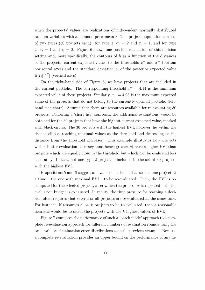
when the projects’ values are realizations of independent normally distributedrandom variables with a common prior mean 3. The project population consistsof two types (50 projects each): for type 1, σi = 2 and τi = 1, and for type2, σi = 1 and τi = 2. Figure 6 shows one possible realization of this decisionsetting and, more specifically, the contours of h as a function of the distancesof the projects’ current expected values to the thresholds x− and x+ (bottomhorizontal axes) and the standard deviation ρi of the posterior expected valueE[Vi|V E

i ] (vertical axes).On the right-hand side of Figure 6, we have projects that are included in

the current portfolio. The corresponding threshold x+ = 4.14 is the minimumexpected value of these projects. Similarly, x− = 4.03 is the maximum expectedvalue of the projects that do not belong to the currently optimal portfolio (left-hand side chart). Assume that there are resources available for re-evaluating 30projects. Following a ‘short list’ approach, the additional evaluations would beobtained for the 30 projects that have the highest current expected value, markedwith black circles. The 30 projects with the highest EVI, however, lie within thedashed ellipse, reaching maximal values at the threshold and decreasing as thedistance from the threshold increases. This example illustrates how projectswith a better evaluation accuracy (and hence greater ρ) have a higher EVI thanprojects which are equally close to the threshold but which can be evaluated lessaccurately. In fact, not one type 2 project is included in the set of 30 projectswith the highest EVI.

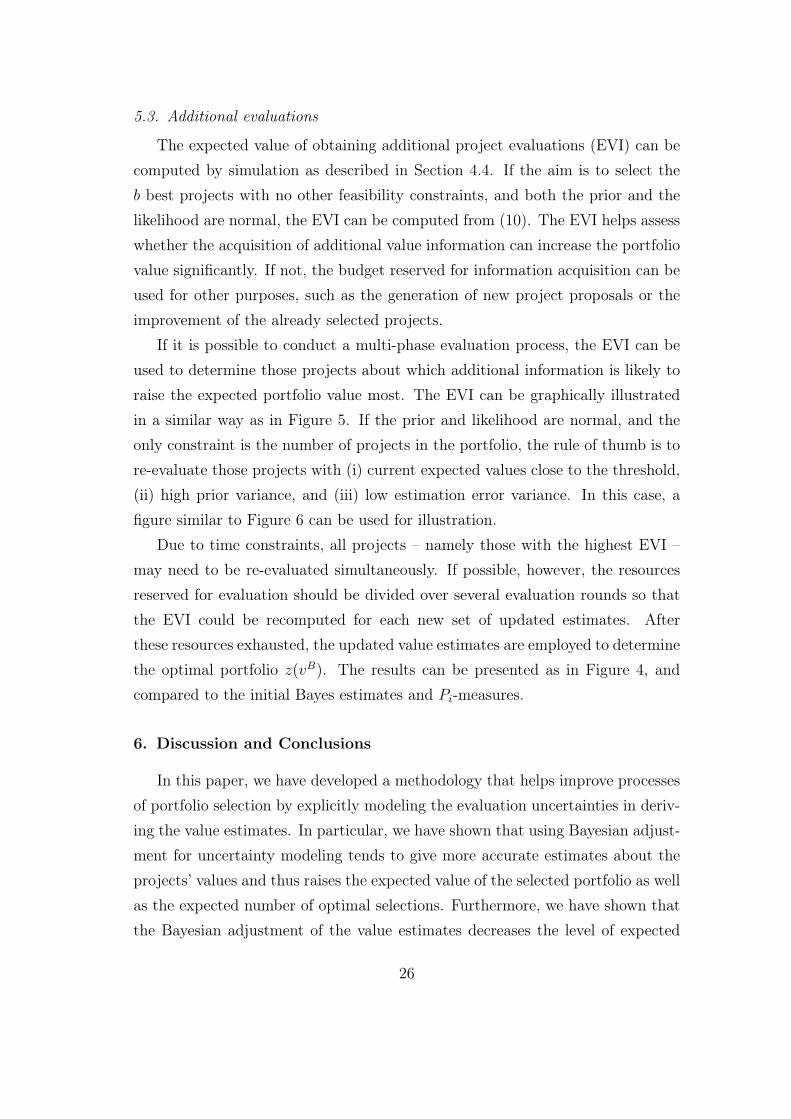
Propositions 5 and 6 suggest an evaluation scheme that selects one project ata time – the one with maximal EVI – to be re-evaluated. Then, the EVI is re-computed for the selected project, after which the procedure is repeated until theevaluation budget is exhausted. In reality, the time pressure for reaching a deci-sion often requires that several or all projects are re-evaluated at the same time.For instance, if resources allow k projects to be re-evaluated, then a reasonableheuristic would be to select the projects with the k highest values of EVI.

Figure 7 compares the performance of such a ‘batch mode’ approach to a com-plete re-evaluation approach for different numbers of evaluation rounds using thesame value and estimation error distributions as in the previous example. Becausea complete re-evaluation provides an upper bound on the performance of any in-

22

complete evaluation scheme, it seems that the batch mode approach is a goodapproximation of the optimal procedure for k evaluations. More importantly, thebatch mode approach seems to yield considerably better results than obtainingadditional evaluations at random. Furthermore, this approach appears to out-perform the often applied ‘short list’ approach of selecting k projects that havethe highest expected values for re-evaluation. Because the three lowest curvesin Figure 7 represent equally expensive evaluation strategies, re-evaluating thoseprojects with the highest EVI is a better strategy in this case than the ‘short list’approach or random selection regardless of the evaluation costs.

1 2 3 491

92

93

94

95

96

97

Number of evaluation rounds

Por

tfolio

val

ue (

% o

f the

opt

imum

)

Complete re−evaluation30 highest EVI30 highest expectationRandom 30

(a) Portfolio value (% of the optimum)

1 2 3 464

66

68

70

72

74

76

78

Number of evaluation rounds

Sha

re o

f opt

imal

sel

ectio

ns (

%)

Complete re−evaluation30 highest EVI30 highest expectationRandom 30

(b) Share of optimal selections (%)

Figure 7: Portfolio value and share of optimal selections with 95% confidence intervals fordifferent numbers of evaluation rounds. Selection of 20 out of 100 projects. Two project types(50% of each): µ = 3, σ1 = 2, σ2 = 1, τ1 = 1, τ2 = 2. 5000 simulation rounds (Monte Carlo).

5. Implications for Decision Support

5.1. Elicitation of the distributions

In the previous sections, we have developed Bayesian methods for modelingvalue and estimation uncertainties in portfolio selection. A prerequisite for theimplementation of these methods is the elicitation of the distributions f(v) (prior)and f(vE|v) (likelihood). Because project portfolio selection is often a recurringactivity in organizations, historical data about the dispersion of the projects’values and about the errors in the value estimates may be available for specifyingthese distributions (Jose, 2010). Nevertheless, if the projects represent completely

23

novel activities, such historical data may not be available, and other estimationmethods are needed.

5.1.1. The prior

To obtain a normal prior, the DM can be asked to specify the prior mean µi

and variance σ2i . If the DM has some information about the location and scale

of the value of project i, it is possible to match these with µi and σ2i . As a rule

of thumb, most of the probability mass (99.9%) lies in the interval I = [µi± 3σi].If the DM can specify some plausible upper and lower bounds for vi, the priormean µi and variance σ2

i can be determined so that these bounds correspond tothe endpoints of interval I (Bolstad, 2007).

In some cases the prior is not normal. For instance, the project values may beasymmetrically distributed with a large part of the probability mass concentratedon smaller values. One possible prior in such cases is the triangular distribution,defined by lower and upper bounds for possible values of vi, and a peak at themost likely value (the mode).

More generally, the DM may be asked to assess the percentiles of the trueproject values vi for each i; i.e., the values below which a certain percentage (e.g.,10%, 20%,. . . ,90%) of observed vi are assumed to fall. The resulting step func-tions can be transformed into continuous distribution functions by using kernelsmoothing methods (e.g. Hastie, Tibshirani, and Friedman, 2009). If the DMdoes not have any prior information about the projects, it is possible to use anuninformative prior (e.g. Price and Manson, 2002). In this case the posteriordistribution is completely determined by the evaluation information.

5.1.2. The likelihood

Often it is plausible to assume that the estimation errors are additive, project-specific, and normally distributed with a zero mean. Then, the specificationof the likelihood corresponds to assessing the estimation error variance τ 2i fori = 1, . . . ,m. To assess τ 2i , the DM can be asked to specify a range within whichshe would expect to see, say, 80% of the estimates given the true value of theproject. Then, τ 2i could be determined to correspond to this range.

Alternatively, if the project is evaluated by multiple experts, the varianceacross the experts’ assessments could be interpreted as τ 2i . Such an approach

24

has been advocated by some researchers (e.g. Gaur et al., 2007). Furthermore,because this method does not require the person(s) evaluating the projects todirectly specify τ 2i , it helps overcome the empirically observed tendency of consis-tently overestimating the precision of one’s value assessments (Liechtenstein andFischhoff, 1977; Kahneman and Tversky, 1979; Soll and Klayman, 2004; Van denSteen, 2011).

As an alternative for assessing τ 2i in the case of normal prior and likeli-hood, Smith and Winkler (2006) suggest that the posterior variance ρ2i is es-timated by asking questions such as: If you had another year and unlimitedresources for additional analysis, how much might the estimate change? If theDM is asked to specify a range (e.g., 10th and 90th percentiles) for the potentialchange, this can be used to estimate ρ2i . Then, by noting that ρ2i = (1 − αi)σ

2i ,

the weight αi of the value estimate in (6) can be readily computed.

5.2. Portfolio selection

Once the necessary distributions have been specified and the value estimatesvE have been observed, the Bayes estimates vB can be computed either throughsimulation (Equation (3)) or, in case of normal prior and likelihood, by usingEquation (6). The Pi-measures can be computed through simulation as describedin Section 4.3 and Equation (9). The recommended portfolio z(vB) can be illus-trated graphically as in Figure 4. By computing the estimated values of bothz(vE) and z(vB), the level of overestimation resulting form the initial estimatesvE can be approximated. Comparison between portfolios z(vE) and z(vB) alsohelps identify those projects that are no longer in the recommended portfolio,because their value estimates have been deflated through Bayesian adjustment.

The variances of the Bayes estimates convey information about the robustnessof the currently optimal portfolio. If the Bayes estimates are very uncertain,additional value information could result in a different optimal portfolio. Here,the Pi-measures are useful: the closer the values of Pi are to either 0 or 1 for all i,the more probable it is that the currently optimal portfolio is truly optimal, andthe less sensitive this portfolio is to additional information. On the other hand,projects that have high Pi-measures but are not included in z(vB) are candidatesfor the elicitation of additional estimates.

25

5.3. Additional evaluations

The expected value of obtaining additional project evaluations (EVI) can becomputed by simulation as described in Section 4.4. If the aim is to select theb best projects with no other feasibility constraints, and both the prior and thelikelihood are normal, the EVI can be computed from (10). The EVI helps assesswhether the acquisition of additional value information can increase the portfoliovalue significantly. If not, the budget reserved for information acquisition can beused for other purposes, such as the generation of new project proposals or theimprovement of the already selected projects.

If it is possible to conduct a multi-phase evaluation process, the EVI can beused to determine those projects about which additional information is likely toraise the expected portfolio value most. The EVI can be graphically illustratedin a similar way as in Figure 5. If the prior and likelihood are normal, and theonly constraint is the number of projects in the portfolio, the rule of thumb is tore-evaluate those projects with (i) current expected values close to the threshold,(ii) high prior variance, and (iii) low estimation error variance. In this case, afigure similar to Figure 6 can be used for illustration.

Due to time constraints, all projects – namely those with the highest EVI –may need to be re-evaluated simultaneously. If possible, however, the resourcesreserved for evaluation should be divided over several evaluation rounds so thatthe EVI could be recomputed for each new set of updated estimates. Afterthese resources exhausted, the updated value estimates are employed to determinethe optimal portfolio z(vB). The results can be presented as in Figure 4, andcompared to the initial Bayes estimates and Pi-measures.

6. Discussion and Conclusions

In this paper, we have developed a methodology that helps improve processesof portfolio selection by explicitly modeling the evaluation uncertainties in deriv-ing the value estimates. In particular, we have shown that using Bayesian adjust-ment for uncertainty modeling tends to give more accurate estimates about theprojects’ values and thus raises the expected value of the selected portfolio as wellas the expected number of optimal selections. Furthermore, we have shown thatthe Bayesian adjustment of the value estimates decreases the level of expected

26

post-decision disappointment, defined as the negative gap between the true andestimated portfolio value. On the other hand, we have shown that by selectingthe portfolio based on initial value estimates alone, the DM should expect to ex-perience post-decision disappointment even if the value estimates were unbiaseda priori.

Recognizing the logic of post-decision disappointment in practical applicationsis important, because otherwise an average negative gap between the true andestimated portfolio value may be interpreted as a systematic underperformance ofprojects, or even as the deliberate misrepresentation of their values and costs. Fly-vbjerg, Skamris Holm, and Buhl (2002), for instance, study the estimated andtrue costs of public transportation infrastructure projects and conclude that thestatistically significant average gap between the true and estimated project costs(ca. 28% for 258 projects, p < 0.001) is best explained by strategic misrepresen-tation by the project promoters, that is, lying. Nevertheless, our results implythat by consistently selecting the projects with the lowest cost estimates withoutexplicitly accounting for estimation uncertainties, the DM is bound to experiencepost-decision disappointment. Against this background, we argue that the under-estimation of the costs of the selected projects can at least in part be attributedto the statistical properties of the value and estimation uncertainties, and notonly to lying or unwarranted optimism.

Apart from its uses in debiasing value estimates, the Bayesian framework isuseful in other ways as well. First, it makes it possible to compute the probabilitywith which a project belongs to the optimal portfolio. This probability serves asa useful project performance measure, because it takes project interdependenciesand other constraints into account. Second, the Bayesian framework makes itpossible to study the value of additional information both analytically and bysimulation; it also helps identify those projects about which additional evaluationsshould be acquired. Our results indicate that it often suffices to re-evaluate onlya subset of the projects. Because the available time and monetary resourcesfor project evaluation are often limited, this result is of considerable practicalinterest.

There are several interesting research directions for the future. For instance,instead of a one-shot decision, portfolio selection can be modeled as a dynamic

27

process, where projects are not only started or rejected, but also sometimes dis-continued to release resources for new projects that offer more value. In such amodeling framework, the analysis of projects with different degrees of uncertain-ties seems particularly interesting, because such differences are likely to suggestdifferent optimal time intervals between project evaluations. Furthermore, theinclusion of risk attitudes will further increase the relevance of this work for prac-tical applications.

Appendix

Proof of Proposition 1: Let us fix v and vE. Then,

z(vE)v − z(vE)vE ≤ z(v)v − z(vE)vE ≤ z(v)v − z(v)vE, (11)

where the first inequality holds because z(v) is the optimal solution to (1) andthe second inequality holds because z(vE) is the optimal solution to (2). Thus,conditioning on V = v and taking expectations of (11) over random V E withdistribution f(vE|v) we have

E[z(V E)v − z(V E)V E|V = v] ≤ E[z(v)v − z(v)V E|V = v] (12)

= z(v)v − z(v)E[V E|V = v]︸ ︷︷ ︸=v

= 0.

with the last equality following from the assumption that the value estimatesare conditionally unbiased. Because (12) holds for all v, we have E[z(V E)V −z(V E)V E] ≤ 0. If there is a possibility of selecting non-optimal projects, i.e.,P(z(V E) ̸= z(V )) > 0, then the first inequality in (11) is strict for some v, vE.Thus, if this event has a positive probability, the inequality in (12) is strict forthe corresponding v, and thus E[z(V E)V − z(V E)V E] < 0�.Proof of Proposition 2: For a given vE, the Bayes estimates vB and the optimalsolutions z(vE) and z(vB) to (2) and (4), respectively, are fixed. The conditionalexpectation of z(vE)V − z(vB)V is

E[z(vE)V − z(vB)V |V E = vE] = z(vE)E[V |V E = vE]︸ ︷︷ ︸=vB

− (13)

−z(vB)E[V |V E = vE]︸ ︷︷ ︸=vB

= z(vE)vB − z(vB)vB ≤ 0,

28

where the second equality follows from the definition of vB, and the last inequalityholds because z(vB) is the optimal solution to (4). Thus, integrating over vE

yields E[z(V E)V − z(V B)V ] ≤ 0. If for some vE we have z(vE) ̸= z(vB), thenz(vE)vB − z(vB)vB < 0 for the corresponding vB = E[V |V E = vE]. Thus, ifP(z(V E) ̸= z(V B)) > 0, then the inequality in (13) is strict and E[z(V E)V −z(V B)V ] < 0 �.Proof of Proposition 3: For a given set of value estimates vE, the Bayesestimates vB and the optimal solution z(vB) to (4) are fixed. The conditionalexpectation of z(vB)V − z(vB)vB is

E[z(vB)V − z(vB)vB|V E = vE] = z(vB)E[V |V E = vE]︸ ︷︷ ︸=vB

−z(vB)vB = 0.

The first equality follows from vB being fixed, and the second from the definitionof vB. By integrating over vE, we have E[z(V B)V − z(V B)V B] = 0 �.Proof of Proposition 4:

E[z(V )z′|V E = vE] =∑

z∗∈{0,1}m[z∗z′P(z(V ) = z∗|V E = vE)]

=∑

z∗∈{0,1}m[

m∑i=1

z∗i ziP(z(V ) = z∗|V E = vE)]

=m∑i=1

[∑

z∗∈{0,1}mz∗i ziP(z(V ) = z∗|V E = vE)]

=m∑i=1

[zi∑

z∗∈{0,1}mP(z(V ) = z∗|V E = vE)z∗i︸ ︷︷ ︸=P(zi(V )=1|V E=vE)

]

=m∑i=1

P(zi(V ) = 1|V E = vE)zi �.

Proof of Proposition 5: Let Z(b) = {z ∈ {0, 1}m|∑m

i=1 zi ≤ b} and z∗ ∈ Z(b)

be such that γ := maxz∈Z(b) zE[V ] = z∗E[V ]. Denote x+ = minj{E[Vj]|z∗j = 1}and x− = maxj{E[Vj]|z∗j = 0}. For any i ∈ {0, ...m}, V E

i , Vj are independent

29

whenever i ̸= j and thus E[Vj|V Ei ] = E[Vj]. Hence by definition

EVI[V Ei ] = E[ max

z∈Z(b)zE[V |V E

i ]]− γ = E[ maxz∈Z(b)

(ziE[Vi|V Ei ] +

m∑j=1j ̸=i

zjE[Vj])]− γ

= E[max{maxz∈Z(b)zi=0

zE[V ],E[Vi|V Ei ] + max

z∈Z(b−1)zi=0

zE[V ]}]− γ. (14)

If z∗i = 0, thenmaxz∈Z(b)zi=0

zE[V ] = γ , maxz∈Z(b−1)

zi=0

zE[V ] = γ − x+,

which can be substituted into (14) to obtain EVI[V Ei ] = E[max{γ,E[Vi|V E

i ]+γ−x−}] − γ = E[max{0,E[Vi|V E

i ] − x−} + γ] − γ = E[max{0,E[Vi|V Ei ] − x−}]. If

z∗i = 1, then

maxz∈Z(b)zi=0

zE[V ] = γ − E[Vi] + x−, maxz∈Z(b−1)

zi=0

zE[V ] = γ − E[Vi],

which can be substituted into (14) to obtain

EVI[V Ei ] = E[max{γ − E[Vi] + x−,E[Vi|V E

i ] + γ − E[Vi]}]− γ

= E[max{x− − E[Vi],E[Vi|V Ei ]− E[Vi]}]

= E[max{x− − E[Vi]− (E[Vi|V Ei ]− E[Vi]), 0}+ E[Vi|V E

i ]− E[Vi]]

= E[max{x− − E[Vi|V Ei ], 0}] + E[E[Vi|V E

i ]]− E[Vi],

where E[E[Vi|V Ei ]] = E[Vi] �.

Proof of Proposition 6: Take any i and denote V Bi = E[Vi|V E

i ]. Using Equa-tion (6) for random V E

i gives V Bi ∼ N(µi, ρ

2i ). Then E[V B

i |V Bi > x+] = µi +

ρiφ(−(x+−µi)

ρi)/Φ(−(x+−µi)

ρi) and E[V B

i |V Bi < x−] = µi − ρiφ(

−(µi−x−)ρi

)/Φ(−(µi−x−)ρi

)

(Sampford, 1953). If z∗i = 0, then x+ − µi ≥ 0, and Proposition 5 implies

EVI[V Ei ] = E

[max{0, V B

i − x+}]= P(V B

i > x+)(E[V B

i |V Bi > x+]− x+

)= Φ

(−(x+ − µi)

ρi

)(µi + ρi

φ(−(x+−µi)ρi

)

Φ(−(x+−µi)ρi

)− x+

)= ρiφ

(−(x+ − µi)

ρi

)− (x+ − µi)Φ

(−(x+ − µi)

ρi

).

Notice that if ρi = 0, then P(V Bi > x+) = 0, wherefore EVI is zero. If z∗i = 1,

30

then µi − x− ≥ 0, and Proposition 5 implies

EVI[V Ei ] = E

[max{0, x− − V B

i }]= P(V B

i ≤ x−)(x− − E[V B

i |V Bi < x−]

)= Φ

(−(µi − x−)

ρi

)(x− − µi + ρi

φ(−(µi−x−)ρi

)

Φ(−(µi−x−)ρi

)

)= ρiφ

(−(µi − x−)

ρi

)− (µi − x−)Φ

(−(µi − x−)

ρi

).

Again ρi = 0 implies that P(V Bi ≤ x−) = 0 and thus EVI is zero. Defining

h : R2+ → R+ such that h(d, ρ) = ρφ(−d/ρ)− dΦ(−d/ρ), if ρ > 0 and h(d, 0) = 0

establishes the main result. To confirm that h is non-negative, decreasing ind and increasing in ρ we write h(d, ρ) = ρΦ(−d/ρ)[φ(−d/ρ)/Φ(−d/ρ) − d/ρ].Because d ≥ 0 and ρ > 0 (omitting the case h(d, 0) = 0), ρΦ(−d/ρ) is clearlypositive, decreasing in d and increasing in ρ. The same can be shown to hold forφ(−d/ρ)/Φ(−d/ρ)− d/ρ (see Sampford 1953 for details). As a product of theseterms, h is nonnegative (with h(d, ρ) = 0 iff ρ = 0), decreasing in d and increasingin ρ. h(0, ρ) = ρ/

√2π follows directly from substitution �.

References

Aguilar, O., M. West. 2000. Bayesian dynamic factor models and portfolio allo-cation. Journal of Business & Economic Statistics 18 338–357.

Arnott, R.D., F. Li, K.F. Sherrerd. 2009. Clairvoyant value and the value effect.Portfolio Management 35 12–26.

Barry, C.B., R.L. Winkler. 1976. Nonstationarity and portfolio choice. The Jour-nal of Financial and Quantitative Analysis 11 217–235.

Bickel, J.E. 2008. The relationship between perfect and imperfect information ina two-action risk-sensitive problem. Decision Analysis 5 116–128.

Bolstad, W.K. 2007. Introduction to Bayesian Statistics (2nd Edition), Wiley,New Jersey.

Brandt, M.W., A. Goyal, P. Santa-Clara, J.R. Stroud. 2005. A simulation ap-proach to dynamic portfolio choice with an application to learning about returnpredictability. Review of Financial Studies 18 831–873.

31

Brown, K.C. 1974. A note on the apparent bias of net revenue estimates forcapital investment projects. Journal of Finance 29 1215–1216.

Chen, S.X., L. Jun. 1997. Statistical applications of the Poisson-binomial andconditional Bernoulli distributions. Statistica Sinica 7 875–892.

Delquié, P. 2008. The value of information and intensity of preference. DecisionAnalysis 5 129–139.

Eeckhoudt, L., P. Godfroid. 2000. Risk aversion and the value of information.Journal of Economic Education 31 382–388.

Fink, D. 1997. A compendium of conjugate priors. Technical report. RetreivedJanuary 10, 2012, www.johndcook.com/CompendiumOfConjugatePriors.pdf.

Flyvbjerg, B., M. Skamris Holm, S. Buhl. 2002. Underestimating costs in pub-lic works projects: error or lie? Journal of the American Planning Associa-tion 68 279–295.

Frazier, P.I., W.B. Powell. 2010. Paradoxes in learning and the marginal value ofinformation. Decision Analysis 7 378–403.

Gaur, V., S. Kesavan, A. Raman, M.L. Fisher. 2007. Estimating demand uncer-tainty using judgemental forecasts. Manufacturing & Service Operations Man-agement 9 480–491.

Gelman, A., J.B. Carlin, H.S. Stern, D.B. Rubin. 2004. Bayesian Data Analysis,Second Edition, Chapman & Hall, London, UK.

Golabi, K., C.W. Kirkwood, A. Sicherman. 1981. Selecting a portfolio of so-lar energy projects using multiattribute preference theory. Management Sci-ence 27 174–189.

Gould, J.P. 1974. Risk, stochastic preference, and the value of information. Jour-nal of Economic Theory 8 64–84.

Grushka-Cockayne, Y., B. De Reyck, Z. Degraeve. 2008. An integrated decision-making approach for improving European air traffic management. ManagementScience 54 1395–1409.

32

Harrison, J.R., J.G. March. 1984. Decision making and post-decision surprises.Administrative Science Quarterly 29 26–42.

Hastie, T., R. Tibshirani, J. Friedman. 2009. The Elements of Statistical Learning:Data Mining, Inference, and Prediction, Second Edition. Springer, New York.

Hilton, R.W. 1981. Determinants of information value: Synthesizing some generalresults. Management Science 27 57–64.

Jose, V.R.R. 2010. Assessing probability distributions from data. In: Wiley Ency-clopedia of Operations Research and Management Science, J.J. Cochran, L.A.Cox Jr., P. Keskinocak, J.P. Kharoufeh, J.C. Smith (Eds.). Wiley, New Jersey.

Kahneman, D., A. Tversky. 1973. On the psychology of prediction. PsychologicalReview 80 237–251.

Kahneman, D., A. Tversky. 1979. Intuitive prediction: biases and corrective pro-cedures. In: Studies in the Management Sciences: Forecasting, S. Makridakisand S.C. Wheelwright (Eds.). Springer, New York.

Keisler, J. 2004. Value of information in portfolio decision analysis. DecisionAnalysis 1 177–189.

Keisler, J. 2009. The value of assessing weights in multi-criteria portfolio decisionanalysis. Journal of Multi-Criteria Decision Analysis 15 111–123.

Kleinmuntz, C.E., D.N. Kleinmuntz. 1999. Strategic approaches for allocatingcapital in healthcare organizations. Healthcare Financial Management 53 52–58.

Laffont, J.-J. 1976. Risk, stochastic preference and information evaluation in deci-sions under uncertainty: A comment. Journal of Economic Theory 12 483–487.

Laffont, J.-J. 1980. Essays in the Economics of Uncertainty, Harvard BusinessPress, Boston.

La Valle, I.H. 1968. On cash equivalents and information evaluation in decisionsunder uncertainty – Part I: Basic theory. Journal of the American StatisticalAssociation 36 252–276.

33

Lichtenstein, S., B. Fischhoff. 1977. Do those who know more also knowmore about what they know? Organizational Behavior and Human Perfor-mance 20 159–183.

Liesiö, J., P. Mild, A. Salo. 2007. Preference programming for Robust Port-folio Modeling and project selection. European Journal of Operational Re-search 181 1488–1505.

Liesiö, J., P. Mild, A. Salo. 2008. Robust Portfolio Modeling with Incomplete CostInformation and Project Interdependencies. European Journal of OperationalResearch 190 679–695.

Liesiö, J., A. Salo. 2012. Scenario-Based Portfolio Selection of Investment Projectswith Incomplete Probability and Utility Information. European Journal of Op-erational Research 217 162–172.

Lindstedt, M., J. Liesiö, A. Salo. 2008. Participatory development of a strategicproduct portfolio in a telecommunication company. International Journal ofTechnology Management 42 250–266.

Marschak, J., R. Radner. 1972. Economic Theory of Teams, Yale University Press,New Haven, CT.

Müller, P. 1999. Simulation-based opitmal design. In: Bayesian Statistics 6, J.M.Bernardo, J.O. Berger, A.P. Dawid, A.F.M. Smith (Eds.), pp. 459–474. OxfordUniversity Press, London.

Park, S.Y., A.K. Bera. 2009. Maximum entropy autoregressive conditional het-eroskedasticity model. Journal of Econometrics 150 219–230.

Polson, N.G., B.V. Tew. 2000. Bayesian portfolio selection: an empirical analy-sis of the S&P 500 index 1970-1996. Journal of Business & Economic Statis-tics 18 164–173.

Price, H.J., A.R. Manson. 2002. Uninformative priors for Bayes’ theorem. Ameri-can Institute of Physics Conference Proceedings: Bayesian Inference and Max-imum Entropy Methods in Science and Engineering 617 379–391

34

Salo, A., J. Keisler, A. Morton. 2011. An invitation to portfolio decision analysis.In: Portfolio Decision Analysis: Improved Methods for Resource Allocation, A.Salo, J. Keisler, A. Morton (Eds.). Springer, New York.

Sampford, M.R. 1953. Some inequalities on Mill’s ratio and related functions.The Annals of Mathematical Statistics 24 130–132.

Smith, J.E., R.L. Winkler. 2006. The optimizer’s curse: Skepticism and postde-cision surprise in decision analysis. Management Science 52 311–322.

Soll, J.B., J. Klayman. 2004. Overconfidence in interval estimates. Journal ofExperimental Psychology, 30 299–314.

Soyer, R., K. Tanyeri. 2006. Bayesian portfolio selection with multi-variate ran-dom variance models. European Journal of Operational Research 171 977–990.

Stummer, C., K. Heidenberger. 2003. Interactive R&D portfolio analysis withproject interdependencies and time profiles of multiple objectives. IEEE Trans-actions on Engineering Management 50 175–183.

Van den Steen, E. 2011. Overconfidence by Bayesian-rational agents. ManagementScience 57 884–896.

Winkler, R.L., C.B. Barry. 1975. A Bayesian model for portfolio selection andrevision. The Journal of Finance 30 179–192.

35