BAW Code of Practice - Infozentrum Wasserbau … Code of Practice Principles for the Design of Bank...
200
BAW Code of Practice Principles for the Design of Bank and Bottom Protection for Inland Waterways (GBB) Issue 2010
Transcript of BAW Code of Practice - Infozentrum Wasserbau … Code of Practice Principles for the Design of Bank...

BAW Code of Practice
Principles for the Design of Bank and Bottom Protection for Inland Waterways (GBB) Issue 2010

Karlsruhe ∙ March 2011 ∙ ISSN 2192-9807
BAW Codes of Practice and Guidelines Publisher
Bundesanstalt für Wasserbau (BAW) Kußmaulstraße 17 76187 Karlsruhe, Germany
P. O. Box 21 02 53 76152 Karlsruhe, Germany
Tel.: +49 721 9726-0 Fax: +49 721 9726-4540
[email protected] www.baw.de
No part of this bulletin may be translated, reproduced or duplicated in any from or by any means without the prior permission of the publisher: © BAW 2011

Principles for the Design
of Bank and Bottom Protection
for Inland Waterways
(GBB)
Issue 2010

Principles for the Design
of Bank and Bottom Protection
for Inland Waterways
(GBB)
Published by: Bundesanstalt für Wasserbau (BAW)
Kußmaulstraße 17 ∙ 76187 Karlsruhe ∙ Germany ∙ Phone (+49721) 9726-0 ∙ Fax (+49721) 9726-4540
e-mail: [email protected] ∙ Internet: http://www.baw.de
No part of this document may be translated, reproduced or duplicated in any form or by any
means without the prior permission of the publisher.
© BAW 2011

Principles for the Design of Bank and Bottom Protection for Inland Waterways
Stand 3/2011 GBB 2010 1
Principles for the Design of Bank and Bottom Protection
for Inland Waterways
Status: March 2011

Principles for the Design of Bank and Bottom Protection for Inland Waterways
GBB 2010
Principles for the Design of Bank and Bottom Protection
for Inland Waterways
Authors and Contributors:
ABROMEIT, Uwe BOR, Federal Waterways Engineering and Research Institute (BAW), Karlsruhe Office (until 2005)
ALBERTS, Dirk Dipl.-Ing., Federal Waterways Engineering and Research Institute (BAW), Hamburg Office († 2005)
BARTNIK, Wolfgang LBDir, Waterways Construction Office (Wasserstraßen-Neubauamt) Datteln
1)
FISCHER, Uwe BDir, Federal Ministry of Transport, Building and Urban Development, Bonn
1)
FLEISCHER, Petra BOR, Federal Waterways Engineering and Research Institute (BAW), Karlsruhe Office
FUEHRER, Manfred Dr. rer. nat., formerly Federal Waterways Engineering and Research Institute (BAW), Karlsruhe Office (until 2000)
GESING, Carolin Dipl.-Ing., Federal Waterways Engineering and Research Institute (BAW), Karlsruhe Office
2)
HEIBAUM, Michael LTRDir, Dr.-Ing., Federal Waterways Engineering and Research Institute (BAW), Karlsruhe Office
1)
HOLFELDER, Tilman Dr.-Ing., Federal Waterways Engineering and Research Institute (BAW), Karlsruhe Office (until 2008)
KAYSER, Jan BDir, Dr.-Ing., Federal Waterways Engineering and Research Institute (BAW), Karlsruhe Office
KNAPPE, Gerd Dipl.-Ing., Waterways Construction Office (Wasserstraßen-Neubauamt) Datteln
1)
KÖHLER, Hans-Jürgen Dipl.-Ing., Federal Waterways Engineering and Research Institute (BAW), Karlsruhe Office (until 2006)
LIEBRECHT, Arno Dipl.-Ing., Regional Waterways and Shipping Directorate Centre (WSD Mitte), Hannover
1)
REINER, Wilfried LBDir, Regional Waterways and Shipping Directorate Centre (WSD Mitte)
1)
SCHMIDT-VÖCKS, Dieter FORMERLY LBDir, Regional Waterways and Shipping Directorate Centre (WSD Mitte) (until 2000)
SCHULZ, Hartmut Prof. Dr.-Ing., Universität der Bundeswehr München (until 1996)
SCHUPPENER, Bernd LBDir, Dr.-Ing., Federal Waterways Engineering and Research Institute (BAW), Karlsruhe Office (1996 until 2009)

Principles for the Design of Bank and Bottom Protection for Inland Waterways
GBB 2010
SÖHNGEN, Bernhard BDir Prof. Dr.-Ing., Federal Waterways Engineering and Research Institute (BAW), Karlsruhe Office
SOYEAUX, Renald Dr.-Ing., Federal Waterways Engineering and Research Institute (BAW), Karlsruhe Office
1) contributor of GBB 2004 (German version)
2) contributor of GBB 2010 (German version)

Principles for the Design of Bank and Bottom Protection for Inland Waterways
Status 3/2011 GBB 2010 4
Content
1 Preliminary remarks 8
1.1 Development of the GBB (Principles for the Design of Bank and Bottom Protection for Inland Waterways) 8
1.2 Scope of application 8
1.3 Structure 9
2 Terms and Definitions 11
3 Summary of the hydraulic actions on the banks and bottoms of rivers and canals 16
3.1 General remarks 16
3.2 Currents 16
3.3 Waves 16
3.3.1 General remarks 16
3.3.2 Form and impact of the wave on the bank 18
3.4 The effect of water level drawdown 18
3.4.1 General remarks 18
3.4.2 Slowly falling water level 19
3.4.3 Rapidly falling water level 19
3.5 Groundwater inflow 20
4 Safety and design concept 21
4.1 General remarks 21
4.2 Hydraulic analyses 22
4.2.1 Aspects of the specification of the design values 22
4.2.2 Recommendations for hydraulic design 23
4.2.2.1 Primary wave field 23
4.2.2.2 Secondary wave field 25
4.2.2.3 Propeller jet 25
4.2.2.4 Recommendations for hydraulic design in standard cases 26
4.3 Geotechnical verifications 27
5 Determination of the hydraulic actions 28
5.1 General remarks 28
5.2 Data on waterways 29
5.2.1 Geometry of waterways 29
5.2.2 Geometry of fairways 29
5.2.3 Water level 29
5.3 Data on vessels 29
5.4 Hydraulic actions due to shipping 31
5.4.1 Components 31
Principles for the Design of Bank and Bottom Protection for Inland Waterways
Status 3/2011 GBB 2010 5
5.4.2 Sailing situations 31
5.4.2.1 Sailing at normal speed 31
5.4.2.2 Manoeuvering 32
5.5 Magnitude of ship-induced waves (design situation: “sailing at normal speed”) 34
5.5.1 Hydraulically effective cross section of canals and ships 35
5.5.1.1 Influence of shallow water 35
5.5.1.2 Influence of boundary layers 43
5.5.2 Critical ship speed for canal conditions 44
5.5.3 Mean drawdown and return flow velocity for vessels sailing in the centre of a canal 47
5.5.4 Hydraulic design parameters and geotechnically relevant drawdown parameters for any
sailing position 52
5.5.4.1 Definition of wave height 52
5.5.4.2 Maximum drawdown at bow and associated return flow velocity without the influence of eccentricity 52
5.5.4.3 Maxium drawdown at the stern and associated return flow velocity without the influence of eccentricity53
5.5.4.4 Maximum heights of bow and stern waves due to eccentric sailing 54
5.5.4.5 Slope supply flow 55
5.5.4.6 Determining the critical flow velocities close to the bank where a natural current is present 58
5.5.4.7 Increase in wave heights in the case of vessels sailing with drift 59
5.5.4.8 Drawdown from ship-induced waves 61
5.5.5 Secondary waves 64
5.5.5.1 General remarks 64
5.5.5.2 Calculation of secondary wave heights 67
5.5.5.3 Additional secondary waves in analogy to an imperfect hydraulic jump 69
5.5.5.4 Secondary waves caused by small boats at planing speed and when sailing close to a bank 70
5.5.5.5 Wave run-up 73
5.5.6 Passing and Overtaking 76
5.6 Hydraulic actions on waterways due to flow caused by propulsion (propeller jet) 76
5.6.1 Induced initial velocity of the propeller jet for stationary vessels (ship speed through water vS = 0) 76
5.6.2 Velocity of the propeller jet at ship speed through water vS 0 79
5.6.3 Jet dispersion characteristics 81
5.6.3.1 Standard jet dispersion situations 81
5.6.3.2 Characteristics of the decrease in the main velocity 83
5.6.3.3 Calculation of the distribution of the jet velocity orthogonal to the jet axis 86
5.6.3.4 Multi screw drives 89
5.6.4 Simplified calculation of the maximum near bed velocity 89
5.6.5 Flow velocity at the bed allowing for the surrounding flow field 90
5.6.6 Load due to bow thrusters 92
5.7 Waves in general, wave deformation and water levels 94
6 Hydraulic design of unbound armour stone cover layers 95
6.1 General remarks 95

Principles for the Design of Bank and Bottom Protection for Inland Waterways
Status 3/2011 GBB 2010 6
6.2 Armour stone size required to resist load caused by transversal stern waves 95
6.3 Stone size required to resist flow due to propulsion 96
6.3.1 Stone size required to resist attack from propeller jet 96
6.3.2 Stone size required to limit the depth of scour due to propeller jet 98
6.4 Armour stone size required to resist load due to secondary diverging waves 99
6.5 Stone size required to resist wind waves or the combined load from ship induced waves and wind waves 99
6.6 Stone size required to resist attack by currents 99
6.6.1 Stone size required to resist attack by currents flowing largely parallel to the slope 100
6.6.2 Stone size required to resist load on the slope due to slope supply flow 101
6.7 Stone size required for all types of load 102
6.8 Armour stone sizes and classes 103
6.9 Minimum thickness of the armour layer 105
6.9.1 Minimum thickness as the basis for armour stone dimensioning 105
6.9.2 Minimum thickness of an armour layer for protection purposes 107
6.10 Minimum length of revetment in the bank slope line (partial revetment) 107
6.10.1 General remarks 107
6.10.2 Above the still water level 107
6.10.3 Below the still water level 107
7 Geotechnical design of unbound armour layers 109
7.1 Design principles 109
7.1.1 General remarks 109
7.1.2 Maximum rapid drawdown za 109
7.1.3 Magnitude of the excess pore water pressure u 110
7.2 Local stability of permeable revetments 112
7.2.1 General remarks 112
7.2.2 Guidance on properties of the ground 113
7.2.3 Depth of the critical failure surface dkrit 113
7.2.4 Effective weight density of the armour layer at buoyancy 113
7.2.5 Weight per unit area of the armour layer required to protect slope revetments against sliding failure 114
7.2.5.1 General remarks 114
7.2.5.2 Method of calculation 114
7.2.6 Weight per unit area of the armour layer required to prevent hydrodynamic soil displacement 116
7.2.6.1 General remarks 116
7.2.6.2 Method of calculation 116
7.2.7 Weight per unit area of an armour layer taking into account a toe support 116
7.2.7.1 General remarks 116
7.2.7.2 Failure mechanism 1 at the upper edge of the toe of the revetment 117
7.2.7.3 Failure mechanism 2 with a toe blanket 118
7.2.7.4 Failure mechanism 2 for an embedded toe 122
7.2.7.5 Failure mechanism 2 for a sheet pile wall at the toe 124

Principles for the Design of Bank and Bottom Protection for Inland Waterways
Status 3/2011 GBB 2010 7
7.2.8 Weight per unit area of the armour layer allowing for a suspension of the revetment 126
7.2.8.1 General remarks 126
7.2.8.2 Verification of the external local-bearing capacity 127
7.2.8.3 Verification of the internal load-bearing capacity 128
7.2.9 Slope revetment above the lowered water level 128
7.3 Local stability of impermeable revetments 129
7.3.1 General remarks 129
7.3.2 Weight per unit area of the armour layer of an impermeable revetment to resist uplift 129
7.3.3 Weight per unit area of the armour layer of an impermeable revetment without toe support required
to resist sliding 129
7.4 Verification of the global stability of the water-slide slope 130
8 Hydraulic and geotechnical design of armour layers consisting of partially grouted
armour stones 131
8.1 Hydraulic Design 131
8.2 Geotechnical Design 131
8.2.1 General remarks 131
8.2.2 Local stability of permeable revetments with partially grouted armour layers 131
8.2.3 Local stability of impermeable revetments with partially grouted armour layers 132
8.3 Verification of the global stability of the water-side slope 132
9 Literature 133
10 Nomenclature 144
10.1 Abbreviations 144
10.2 Symbols 144
Annexes
Annex A Calculation methods for geotechnical design for determining the required
weight per unit area of armour layers
Annex B Flow chart for carrying out the geotechnical design
Annex C Determination of an equivalent trapezoidal profile
Annex D Change in the mean return flow velocity between ship and bank for slender
ships and small drawdown
Annex E General jet dispersion for standard situations 1 and 2 and for vS = 0

Principles for the Design of Bank and Bottom Protection for Inland Waterways
Status 3/2011 GBB 2010 8
1 Preliminary remarks
1.1 Development of the GBB (Principles for the Design of Bank and Bottom
Protection for Inland Waterways)
This publication describes in detail the principles of the design of bank and bottom protection for inland waterways, taking into account the results of the latest research. The principles include the verification by calculation of the stability and resistance to erosion of canal embankments and, with certain limitations, the banks of rivers exposed to natural hydraulic influences and to those caused by shipping.
The first version of the GBB was published in 2004 /BAW 2005/, when for the first time comprehensive principles for the design of bank and bottom protection for inland waterways became available. Since then, the GBB have successfully and diversely been implemented in large numbers of projects for the dimensioning of bank and bottom protection.
The Code of Practice “Use of Standard Construction Methods for Bank and Bottom Protection on Inland Waterways (MAR)” was revised on the basis of the GBB, and extensive calculations according to the GBB were carried out for this purpose. The revised MAR was published in 2008 /MAR 2008/. The MAR enables the dimensioning of bank and bottom protection under defined boundary conditions and without the need for further calculations.
Furthermore a working Group of the BAW and WSV developed the software GBBSoft /BAW 2008/, which was completed in the year 2008 and enables the uncomplicated application of the GBB. Further facts regarding design were established during research and development work with the help of theoretical observations and studies from models and in the field.
Now after six years of intensive use of the GBB it was time to revise them to include new information in the application and to correct errors that had been identified. During the revision work, the following principal amendments were made:
additions to the calculation principles for the diminishing of drawdown between ship and bank
revision of the design formulae for scouring as a result of propeller jet
generalisation of the jet dispersion from multi-screw drives
consideration of velocities greater than the planing speed of recreational craft
consideration of varying flow velocities at bottom and bank in the design of stone size
introduction of a weighting concept that allows for differing methods for determining armour stone size
more precise structuring with regard to geotechnical and hydraulic calculations
summary of the impact of differing waves and the elimination of wind waves (Note: These waves usually cause less impact than ship-induced waves; they are seldom relevant to the design. Regarding this point we merely refer to the GBB from 2005 /BAW 2005/. The corresponding chapters there retain their validity.)
Adjustment to stone classes according to /DIN EN 13383/.
Expanded definition of minimum thicknesses and elimination of hydraulically equivalent armour layer thicknesses
revision of the global stability of the water-side slope
expansion of the appendices for better understanding of the theoretical background
The revised GBB is herewith made available as the GBB 2010.
1.2 Scope of application
The scope of the hydraulic design approaches primarily covers waterways with predominantly parallel banks (prismatic cross sections), with fairways confined both laterally and in depth, with depths that are virtually constant except in the vicinity of the banks (i.e. no berms), with a maximum ratio of the water surface width to ship’s length (bws/L) of around 2:1 and with shipping traffic (including recreational craft) that causes displacement that would influence the design of the armour layers. Within certain limitations, the methods described can also be applied to widened stretches of canals and waterbodies regulated by impoundments, if vessels sail close to the banks and those banks are regular, i.e. without any projections or funnels where
Principles for the Design of Bank and Bottom Protection for Inland Waterways
Status 3/2011 GBB 2010 9
ship-induced waves can accumulate. Within these limitations, the influence of the shape of the bank, the turbulence and the current on wave propagation can be disregarded. The influence of shallow water (i.e. if bws/L is greater than 2/1) on possible ship speeds and drawdown in the vicinity of ships can be taken into account by approximation by allowing for an equivalent canal cross section. Approximation equations have been included for the calculation of the decrease in wave height as the waves move away from a vessel. Approximation methods are also used to estimate the hydraulic actions caused by recreational craft and craft with short stocky hulls (such as pusher craft and tugs).
Methods of calculating the hydraulic design parameters (wave height, flow velocity) described in chapter 5 do not cover the following situations:
extremely variable sequence of cross sections and waterways with irregular banks
unconventional propulsion such as Schottel propellers or jet propulsion
non-displacement craft such as hovercrafts
sea-going vessels and other vessels whose design differs from the usual design of inland navigation vessels, e.g. ships with bulbous bows (These give rise to different types of secondary waves.)
depth-based Froude numbers 8.0mS hgv (Here the secondary wave system is altered significantly.)
the course of a vessel of which the sailing line deviates considerably from the axis of the canal (causing pronounced changes in the primary and secondary wave systems)
Design procedures based on readings, e.g. for ship-induced wave heights, if available, can be applied directly when determining the size of armour stones (see chapter 6).
The following points are not covered by the procedure for determining the size of armour stones given in chapter 6. (This does not affect the geotechnical design process.):
banks with gradients of less than approx. 1:5 (at which significant deformation of the incoming waves occurs) and greater than approx. 1:2
wave deformation at the slope (although this is taken into account indirectly in the design procedures covering wave heights at the toe of the slope)
slope revetments comprising shaped stones, gabions or asphalt
1.3 Structure
This current GBB 2010 is divided into three main sections:
The first section includes definitions of the relevant terminology, explanations of the hydraulic and geotechnical principles and an introduction to the safety philosophy and the design concept (see chapters 2 to 4).
The second section deals with the determination of the hydraulic actions that constitute the input parameters for the design (see chapter 5).
The third section deals with hydraulic and geotechnical design procedures (see chapters 6 to 8).
The design of bank and bottom protection comprises a hydraulic and a geotechnical component (see Figure 1.1). The two design components must be carried out separately.

Principles for the Design of Bank and Bottom Protection for Inland Waterways
Status 3/2011 GBB 2010 10
Figure 1.1 Main components of the design of bank and bottom protection
Hydraulic design deals with the determination of the required individual stone size of a revetment consisting of loose armour stones, depending on the load from waves and current. The purpose of geotechnical design is to establish the required mass per unit area of the revetment to ensure adequate resistance to sliding failure, uplift and hydrodynamic soil displacement. In addition to this, a geotechnical verification of the overall stability of the slope including the revetment is required.
Finally, the results of hydraulic and geotechnical design serve as the basis for determining the required minimum thickness of armour layers. It must also be checked whether sufficient protection is ensured in the event of ship impact as well as anchor drop and ultraviolet radiation, and that the filtration length is sufficient to safeguard against the transport of particles.
The methods described in this publication apply in conjunction with the latest versions of the following codes and guidelines for bank and bottom protection on waterways
- BAW Code of Practice "Use of Standard Construction Methods for Bank and Bottom Protection on Inland Waterways (MAR)" /MAR 2008/
- BAW Merkblatt „Anwendung von Kornfiltern an Wasserstraßen (MAK)“ /MAK 1989/ [BAW Code of Practice: "Use of Gravel Filters on Waterways"; only in German language]
- BAW Code of Practice "Use of Geotextile Filters on Waterways (MAG)" /MAG 1993/
- BAW Code of Practice "Use of Cementitious and Bituminous Materials for Grouting Armourstone on Waterways (MAV)" /MAV 2008/
- Technische Lieferbedingungen für Wasserbausteine /TLW 2003/ ["Technical Supply Conditions for Armourstones"; only in German language]
- Richtlinien für Regelquerschnitte von Schifffahrtskanälen /BMV 1994/ ["Guidelines for Standard Cross Sections of Shipping Canals"; only in German language]
Geotechnical Design
statically required thickness of armour layer
Design results
Required size or weight of individual armour stones
Required thickness of the armour layer as a maximum of the geotechnical design and the minimum thickness
Hydraulic Design
Size of individual stones
Minimum thickness of the armour layer

Principles for the Design of Bank and Bottom Protection for Inland Waterways
Status 3/2011 GBB 2010 11
2 Terms and Definitions
Advance ratio of a propeller: Ratio J of the velocity of the approach flow towards the propeller vA to the product of the propeller speed n and propeller diameter D (J = vA/nD).
Armour layer: The upper layer of a revetment; it must be resistant to erosion and have adequate resistance to anchor drop or ship impact.
Bow swell (‘swell-up’ at the bow): Accumulation of water in front of the bow over the influence width, caused by vessels accelerating or when sailing steadily along canals with rough beds (water surface elevation); unlike
bow waves, bow swell occurs over large widths (canal width) (see Figure 2.1).
Bed: Wetted perimeter of a canal or river, consisting of the bed and banks.
Blockage ratio: The ratio n of the cross-sectional area A of a waterway at a particular water level (which affects the return flow) to the cross-sectional area AM of the submerged part of a vessel (n = A/AM). In the literature in Britain and North America the blockage coefficient k = 1/n, the reciprocal value of the cross section ratio n or blockage ratio, is generally used.
Bow thruster: A ship’s propeller (standard model) that accelerates water in a tube in the bow section orthogonal to the axis of the vessel. It exerts a transversal thrust that acts in the same way as a rudder. It is most effective at low ship speeds over ground.
Bow wave: Accumulation of approaching water directly in front of the bow of a vessel (stagnation point) that
gives rise to the formation of secondary waves on either side of the vessel.
Breaking of waves: A wave will break when the wave steepness reaches a critical value as a result of
wave shoaling. The process is accompanied by the formation of a water-air mix and a loss of wave energy
( plunging breakers).
Breaking waves: Breaking of waves
Figure 2.1 Deformation of water surface in the direction of travel, squat and direction of return flow (vector arrows) for a conventional inland navigation vessel with a full bow as described by /Kuhn 1985/
(a) Lowered water level and ship-induced waves
1 vessel at rest, 2 vessel in motion, 3 still-water level, 4 lowered water level (primary wave), 5 superimposed secondary wave, 6 bow swell, 7 stern wave, 8 return flow,
Δt squat,tfl dynamic underkeel clearance,tv draught of vessel while sailing,
(b) (-) trim angle, bow-heavy
(c) (+) trim angle, stern-heavy
(b) and (c) without deformation of the water surface

Principles for the Design of Bank and Bottom Protection for Inland Waterways
Status 3/2011 GBB 2010 12
Canal conditions: Confined waterway (with restricted depth and width). Canals are the most common type of inland waterway.
The effect of the width limit (“canal condition”) becomes noticeable when the ratio of the water surface width bWS to the length of the vessel L becomes bWS/L ≤ 2-3 /Schuster 1952/.
Canal conditions exist at low blockage ratios. As a rough approximation, n = A/AM ≤ 25–35 for motor vessels and large inland cargo vessels, the higher value applying to long, narrow vessels with a shallow draught and the lower value to short, wide vessels with a deep draught.
Cross section ratio blockage ratio
Deep water: Waves can propagate or diminish entirely unhindered due to the absence of any depth or width restriction; this situation obtains in large, deep lakes and in seas.
Depth, critical: The depth at which a failure surface parallel to and close to the surface of a slope occurs in the
underlying soil after the shear resistance of the soil has been reduced to a minimum as a result of the excess
pore water pressure caused by rapid drawdown ( local stability).
Diffraction: Occurs when a wave front hits an obstacle. As each point of a wave crest is the starting point for new circular wavelets, waves are generated at the end of the obstacle that is exposed to waves and propagate on its lee side. The wave celerity is not altered but the wave height and direction change at the open flanks.
Diverging waves: These form part of the secondary wave system in which the wave crests diverge at an acute angle to the vessel’s direction of travel.
Drawdown velocity: Average rate at which the water level falls at any point on a bank.
Drawdown, rapid: Drawdown in which the rate at which the water level drops is higher than the permeability of the bed and banks of the river or canal.
Drawdown: Lowering of the water level adjacent to a vessel caused by the displacement flow.
Ducted propeller: Propeller enclosed in a cylindrical duct to increase its efficiency.
Excess pore water pressure: The water pressure in the pores of a soil in excess of the hydrostatic pore water pressure, which arises when the volume of the pore water is prevented from increasing (if the pore water pressure changes) or when the volume of the granular structure is prevented from decreasing (if there are
changes in the total or effective tension of the granular structure). It is caused by rapid drawdown. As a result, the pressure in the subsoil is higher than at the water/soil interface.
Fetch: Area of the surface of a body of water in which wind waves can be generated. The effective fetch takes into account any restrictions in length or width owing to topographical features (such as banks or islands) and/or meteorological conditions (e.g. wind direction).
Influence width (~, effective): The effective influence width bE is the imaginary width in which the entire return flow field around a vessel is concentrated. It enables the maximum drawdown and return flow velocities of vessels sailing in shallow water to be calculated for an equivalent waterway cross section of the same width.
Manoeuvring situation: Navigation at low speed for the purposes of manoeuvring vS ~ 0, i.e. at an advance ratio of the propeller of J ~ 0 and maximum propeller thrust loading (for starting, stopping and turning).
Midship section, submerged: Maximum submerged cross-sectional area of a vessel at rest (beam multiplied by the draught).
n-ratio: Cross section ratio
Planing speed: Speed at which a vessel (recreational craft) begins to slide and ride up on its own bow wave.
Plunging breaker: The velocity of approaching waves decreases close to the ground as the water becomes shallower; at the same time, the steepness of the wave front increases without any significant absorption of air. Intensive absorption of air occurs when the wave front is more or less vertical and the wave front plunges. When a plunging wave hits a bank, it breaks with substantial force as a result of the compressibility of the absorbed air, and loses a great amount of its energy. This type of breaker can be observed at steep banks.
Positive surge / drawdown waves: Variations in the water level are caused by sudden changes in the flow of water owing to the operation of the waterway. They are similar to single waves in shallow water.

Principles for the Design of Bank and Bottom Protection for Inland Waterways
Status 3/2011 GBB 2010 13
Primary wave (primary wave system): Consequence of the interaction between a vessel and the waterway as a result of the flow around the hull due to displacement. The lowering of the water level on either side of the vessel and the bow swell and stern are part of the displacement flow. The primary wave system surrounds the vessel and travels with it; the waves decline as they move away from the ship’s hull (see Figure 2.2 and Figure 2.3).
Reflection: When waves strike a boundary surface (wall, groyne, training wall, steep bank, etc.) they are partially reflected, resulting in a loss of wave energy. The height of the reflected wave is usually lower than that of the incoming wave. Incoming waves and reflected waves are superimposed on each other.
Refraction: Change in the direction and magnitude of a wave front owing to friction on the river or canal bed caused by a change in the depth of the water in the vicinity of a bank. Applies to waves that initially travel parallel and are refracted towards the bank, and to ship-induced secondary waves which are already running at
a diverging angle. One side of the wave crest is in shallower water than the other. As the velocity of shallow water waves diminishes with the depth of the water, the wave flank closest to the bank moves more slowly than
the flank furthest away from the bank, resulting in curvature of the wave crest. Refraction causes the wave
height to diminish. Refraction is accompanied by wave shoaling.
Return flow: Water flowing in the opposite direction to the vessel; it is caused by the displacement action of the vessel and drawdown.
Revetment: Permeable or impermeable lining of a waterway intended to prevent changes in its bed and banks.
Running wave: When transversal stern waves travelling along a bank break they are referred to as running waves; they are particularly high when a vessel approaches its critical speed.
Sailing at normal speed: Navigation at a speed permitted on open stretches of canals in the Regulations for Navigation on Inland Waterways or at a technically feasible ship speed.
Sailing line: Position of the actual axis of the path of a vessel in relation to the axis of the waterway.
Secondary waves (secondary wave system): Regular, short-periodic waves, which are known as secondary waves, develop simultaneously at the bug and stern of the ship because of the changes in contour of the hull of the ship. On the one hand, these are diverging waves, which spread out at an angle to the axis of the ship and, on the other, transverse waves, which are aligned almost perpendicularly to the ship’s axis. The superimpos ition of the two systems produces an interference line, which, depending on the speed of the vessel, has a characteristic angle to the ship’s axis: at normal ship speeds this angle is 19.47°. (see Figure 2.2 and Figure 2.3).
Figure 2.2 Deformation of the water surface (top view). Least favourable superimposition of primary and secondary wave systems.
Principles for the Design of Bank and Bottom Protection for Inland Waterways
Status 3/2011 GBB 2010 14
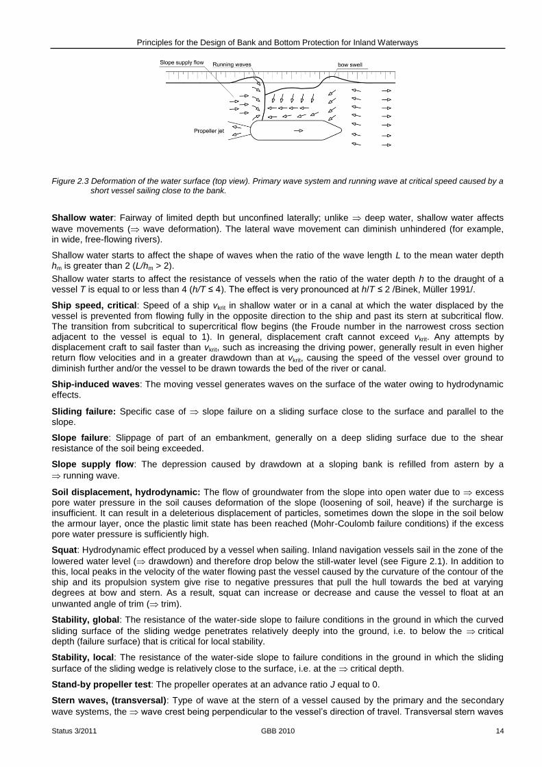
Figure 2.3 Deformation of the water surface (top view). Primary wave system and running wave at critical speed caused by a short vessel sailing close to the bank.
Shallow water: Fairway of limited depth but unconfined laterally; unlike deep water, shallow water affects
wave movements ( wave deformation). The lateral wave movement can diminish unhindered (for example, in wide, free-flowing rivers).
Shallow water starts to affect the shape of waves when the ratio of the wave length L to the mean water depth hm is greater than 2 (L/hm > 2).
Shallow water starts to affect the resistance of vessels when the ratio of the water depth h to the draught of a vessel T is equal to or less than 4 (h/T ≤ 4). The effect is very pronounced at h/T ≤ 2 /Binek, Müller 1991/.
Ship speed, critical: Speed of a ship vkrit in shallow water or in a canal at which the water displaced by the vessel is prevented from flowing fully in the opposite direction to the ship and past its stern at subcritical flow. The transition from subcritical to supercritical flow begins (the Froude number in the narrowest cross section adjacent to the vessel is equal to 1). In general, displacement craft cannot exceed vkrit. Any attempts by displacement craft to sail faster than vkrit, such as increasing the driving power, generally result in even higher return flow velocities and in a greater drawdown than at vkrit, causing the speed of the vessel over ground to diminish further and/or the vessel to be drawn towards the bed of the river or canal.
Ship-induced waves: The moving vessel generates waves on the surface of the water owing to hydrodynamic effects.
Sliding failure: Specific case of slope failure on a sliding surface close to the surface and parallel to the slope.
Slope failure: Slippage of part of an embankment, generally on a deep sliding surface due to the shear resistance of the soil being exceeded.
Slope supply flow: The depression caused by drawdown at a sloping bank is refilled from astern by a
running wave.
Soil displacement, hydrodynamic: The flow of groundwater from the slope into open water due to excess pore water pressure in the soil causes deformation of the slope (loosening of soil, heave) if the surcharge is insufficient. It can result in a deleterious displacement of particles, sometimes down the slope in the soil below the armour layer, once the plastic limit state has been reached (Mohr-Coulomb failure conditions) if the excess pore water pressure is sufficiently high.
Squat: Hydrodynamic effect produced by a vessel when sailing. Inland navigation vessels sail in the zone of the
lowered water level ( drawdown) and therefore drop below the still-water level (see Figure 2.1). In addition to this, local peaks in the velocity of the water flowing past the vessel caused by the curvature of the contour of the ship and its propulsion system give rise to negative pressures that pull the hull towards the bed at varying degrees at bow and stern. As a result, squat can increase or decrease and cause the vessel to float at an
unwanted angle of trim ( trim).
Stability, global: The resistance of the water-side slope to failure conditions in the ground in which the curved
sliding surface of the sliding wedge penetrates relatively deeply into the ground, i.e. to below the critical depth (failure surface) that is critical for local stability.
Stability, local: The resistance of the water-side slope to failure conditions in the ground in which the sliding
surface of the sliding wedge is relatively close to the surface, i.e. at the critical depth.
Stand-by propeller test: The propeller operates at an advance ratio J equal to 0.
Stern waves, (transversal): Type of wave at the stern of a vessel caused by the primary and the secondary
wave systems, the wave crest being perpendicular to the vessel’s direction of travel. Transversal stern waves

Principles for the Design of Bank and Bottom Protection for Inland Waterways
Status 3/2011 GBB 2010 15
caused by primary and secondary wave systems may be superimposed on each other. Running waves are a particular type of transversal stern wave (see Figure 2.1).
Superposition of waves: When waves of different origins, directions or celerities meet, their heights are superimposed on each other if the wave heights are small in proportion to the depth of the water.
Toe protection: Lower part of a slope revetment.
Transversal waves: These form part of the secondary wave system in which the wave crests are perpendicular to the direction of travel of the vessel.
Trim, dynamic: Additional inclination of the longitudinal axis of a vessel in relation to the horizontal, caused by
dynamic processes occurring while the vessel is in motion ( squat).
Trim, static: A greater draught at the bow than at the stern can be chosen for safety reasons to ensure that the bow of the vessel (not the stern) touches the bed first at shallows in bodies of water with moving beds, e.g. rivers.
Water depth, mean: Calculated depth of a waterway obtained by dividing the flow cross section by the water surface width.
Some important terms relating to the hydraulic features of rivers and canals as well as to the dimensions of waterways and fairways as used in this publication are shown in Figure 2.4.
Figure 2.4 Dimensions of canal and fairway according to /Kuhn 1985/ 1 canal cross section or bed relevant to the design, bF width of fairway, bWS water surface width, h' depth of
fairway, h water depth, T draught, Δt squat, tv draught while sailing = T + Δt, tf underkeel clearance = h' - T, tfl dynamic under-keel clearance, tfl,min minimum dynamic under-keel clearance, A canal cross section, AM submerged midship section of vessel, lu wetted perimeter of canal (without vessel), BW operating water level
Water depth-to-draught ratio: Ratio of the water depth h to the draught of a vessel T (h/T).
Wave crest: Peak line of a wave orthogonal to its direction of propagation.
Wave deformation: Changes in the wave crest, and in particular in the wave height, will occur if waves are
unable to propagate unhindered (for example, as a result of variations in the water depth caused by shallow water, beds of rivers or canals, structures, approach angles etc.). The principal types of deformation are
wave shoaling, breaking, diffraction, refraction and reflection.
Wave height: A definition of wave height of regular waves or specified design waves is the vertical difference between a trough and the preceding crest, for example. The length of time between these two points is half a wave length or wave period. Statistical methods can be used to determine the design wave height of natural, irregular waves.
Wave length: Defined, for example, as the horizontal distance between two wave crests or troughs for regular waves or specified design waves. Statistical methods can be used for natural, irregular waves.
Wave run-up: Occurs when a wave, either broken or unbroken, runs up the bank for a certain distance.
Wave shoaling: Waves in shallow water are always in contact with the bed. A reduction in the depth of the water causes a decrease in the wave celerity and the wave length as well as an increase in the wave height
with the wave period remaining constant. The front and back of the wave become steeper. Refraction also occurs when waves run up a bank at an oblique angle.
Wave steepness: Ratio of wave height to wave length. It is a variable geometrical parameter for waves.
Wind set-up: Rise in the water level in the lee of a fetch caused by shear stress between the air flow and the surface of the water during constant wind action over a relatively long period of time.
Wind waves: Waves caused by the action of the wind on the surface of the water.
Principles for the Design of Bank and Bottom Protection for Inland Waterways
Status 3/2011 GBB 2010 16
3 Summary of the hydraulic actions on the banks and bottoms of rivers
and canals
3.1 General remarks
The bottoms and banks of rivers and canals are exposed to the following hydraulic actions, that can occur alone or at the same time:
- currents
- waves
- drawdown
- groundwater inflow
Currents and waves can cause erosion of the bottoms and banks of a canal or river, while rapid drawdown or a considerable inflow of groundwater may result in sliding or loosening of the soil (heave).
The resistance of the bottoms and banks of rivers and canals to such hydraulic actions must be verified if any changes to the cross section of the waterway are unacceptable. Protection must be provided for banks and/or bottoms if resistance (stability) is inadequate.
3.2 Currents
Only turbulent currents are of significance for waterways. They can cause erosion, depending on the particle size of the material present in the banks and beds. Highly turbulent currents occur, in particular, in:
- the tail water of weirs
- the propeller jet of ships
- the return flow caused by shipping
- the slope supply flow
3.3 Waves
3.3.1 General remarks
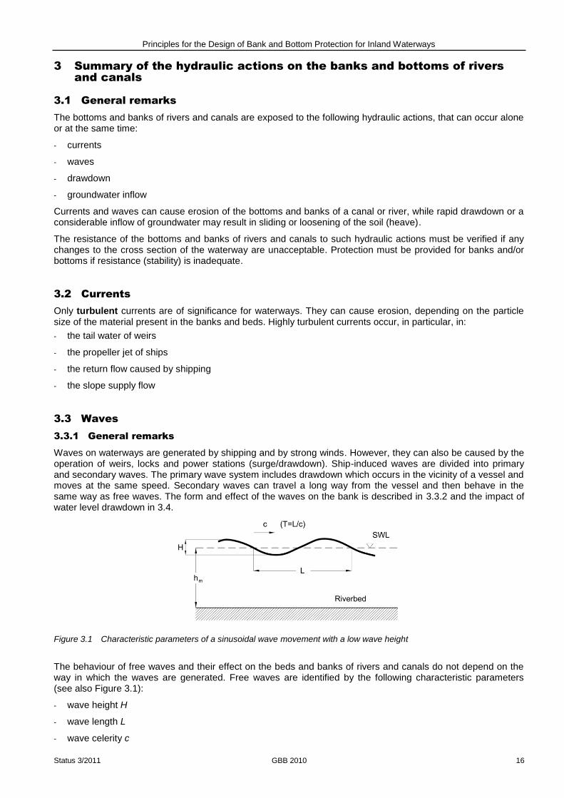
Waves on waterways are generated by shipping and by strong winds. However, they can also be caused by the operation of weirs, locks and power stations (surge/drawdown). Ship-induced waves are divided into primary and secondary waves. The primary wave system includes drawdown which occurs in the vicinity of a vessel and moves at the same speed. Secondary waves can travel a long way from the vessel and then behave in the same way as free waves. The form and effect of the waves on the bank is described in 3.3.2 and the impact of water level drawdown in 3.4.
Figure 3.1 Characteristic parameters of a sinusoidal wave movement with a low wave height
The behaviour of free waves and their effect on the beds and banks of rivers and canals do not depend on the way in which the waves are generated. Free waves are identified by the following characteristic parameters (see also Figure 3.1):
- wave height H
- wave length L
- wave celerity c
Principles for the Design of Bank and Bottom Protection for Inland Waterways
Status 3/2011 GBB 2010 17
- wave period T
- mean water depth hm
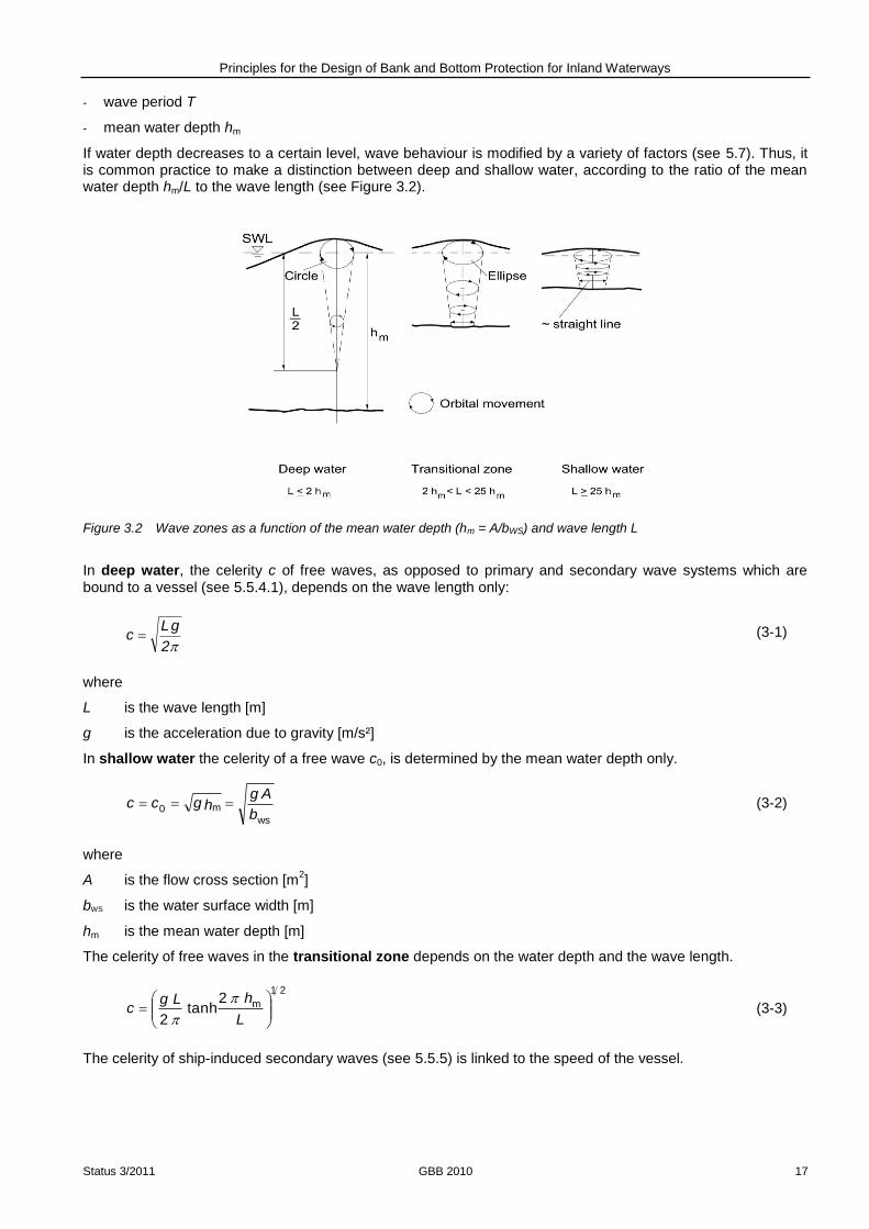
If water depth decreases to a certain level, wave behaviour is modified by a variety of factors (see 5.7). Thus, it is common practice to make a distinction between deep and shallow water, according to the ratio of the mean water depth hm/L to the wave length (see Figure 3.2).
Figure 3.2 Wave zones as a function of the mean water depth (hm = A/bWS) and wave length L
In deep water, the celerity c of free waves, as opposed to primary and secondary wave systems which are bound to a vessel (see 5.5.4.1), depends on the wave length only:
2
gLc
(3-1)
where
L is the wave length [m]
g is the acceleration due to gravity [m/s²]
In shallow water the celerity of a free wave c0, is determined by the mean water depth only.
ws
m0b
Ag hgcc (3-2)
where
A is the flow cross section [m2]
bWS is the water surface width [m]
hm is the mean water depth [m]
The celerity of free waves in the transitional zone depends on the water depth and the wave length.
21
m2tanh
2
L
hLgc
(3-3)
The celerity of ship-induced secondary waves (see 5.5.5) is linked to the speed of the vessel.

Principles for the Design of Bank and Bottom Protection for Inland Waterways
Status 3/2011 GBB 2010 18
In general, according to /Press, Schröder 1966/, the following distinctions are sufficient for practical calculations:
Deep water: hm / L
≥ 0.5
Shallow water: hm / L
< 0.5
Accordingly, ship-induced secondary waves are generally to be regarded as deep water waves and the primary wave due to drawdown as a shallow water wave.
3.3.2 Form and impact of the wave on the bank
Unbroken wave travelling with the ship
When an unbroken wave passes in the longitudinal direction of the bank, rapid hydrostatic pressure changes occur at the slope, to which the pore water pressure in the subsoil cannot adapt as quickly (see 3.4). The pore water pressure in the soil may be greater or less than the external hydrostatic pressure (i.e. caused by wave troughs or wave crests), depending on the water level at any given moment, giving rise to a flow of water into or out of the subsoil. The flow of pore water out of the subsoil reduces the weight of individual soil particles, which has already been diminished by buoyancy, and may cause loosening of the soil. It may promote erosion if actions due to flow occur at the same time.
In transitional zones and in shallow water zones, the orbital movement of a wave can give rise to a reciprocating motion in individual soil particles, causing them, and also small armour stones, to shift slightly. A significant degree of erosion does not occur until the flow forces reach a level at which they transport away the material that has been set in motion.
Breaking run-up wave
Free waves and secondary ship-induced waves can run up in a direction transverse to the bank and break. The type of breaker described in GBB 2004 /BAW 2005/ depends largely on the inclination of the slope. The stability of the bank (zone of fluctuating water levels) is especially impacted by plunging breakers, as the plunging water and the resulting run-up and run-down have a highly erosive effect (displacement of stones) through their flow force and high level of turbulence. The resulting hydraulic shock also causes excess pore pressure in the saturated subsoil, which may be several times the hydrostatic head of the waves. Its effect is relatively small if the waves break in a water cushion or an armour layer with a large number of cavities (e.g. rip-rap). Only several hydraulic shocks in close succession can reduce the stability of the bank slope, because the excess pore water pressure in the soil is unable to diminish quickly enough, thus lowering the shear strength.
Breaking wave travelling with the ship
A wave travelling with the ship parallel to a bank at the stern of a vessel (transversal stern wave) may break – depending on the wave steepness and the Froude number or the ratio of the ship speed to the critical speed – (running wave or slope supply flow). The locally high velocity of the slope supply flow can lead to the displacement of armour stones.
3.4 The effect of water level drawdown
3.4.1 General remarks
Natural or man-made influences can cause the water level of a river or canal to change slowly or rapidly. The geotechnical stability of the banks and bottom is primarily dependent on whether the pore water in the underlying soil is able to adapt to the changes in the water level of the river or canal without significant excess pressures being generated.
A comparison of the drawdown rate of the water level (vza) and the permeability of the soil (k) can provide a first conservative estimate of whether excess pore water pressure is being generated.
(a) slowly falling water level: vza < k
(b) rapidly falling water level: vza < k

Principles for the Design of Bank and Bottom Protection for Inland Waterways
Status 3/2011 GBB 2010 19
3.4.2 Slowly falling water level
In the soil of the bed and banks of a river or canal, the decrease in the hydrostatic pore water pressure is always delayed when drawdown occurs, as pore water can only flow out of a slope if a pressure differential exists.
If the drawdown rate is less than the permeability of the soil of the bed and banks (vza < k), the possible gradient is also small, and the pore water pressure is only slightly above that of the free water level that is acting at that particular moment. The associated flow force can be disregarded with respect to the stability of the banks and the bed of the waterway.
3.4.3 Rapidly falling water level
Excess pore water pressure in the soil occurs when the rate at which the water level falls exceeds the rate at which the hydrostatic pore water pressure in the soil is able to adapt (vza ≥ k). Excess pore water pressure is caused by the delay in pressure equalization owing to gas bubbles that increase in size as the pressure decreases. /Köhler 1993/;/Köhler 1997/
The excess pore water pressure gives rise to seepage flow towards the ground surface (see Figure 3.3). The effective stresses in the soil and, thus, the frictional forces, may be reduced, causing static limit states to occur. Then sliding failure may occur in banks (with or without a revetment) along a failure interface parallel to the slope at the depth dkrit (see 7.2.3) or loosening of the soil may occur near the surface (“hydrodynamic displacement of the soil”) of the slope or of the bed (see Annex A).
The provision of a sufficiently heavy revetment that is dimensioned principally by the density of the armour stones and by the revetment thickness can prevent such limit states occurring in the ground.
Figure 3.3 Flow lines and equipotential lines in the ground below a permeable slope revetment during rapid drawdown of the water level
The magnitude and development of excess pore water pressure due to rapid drawdown are governed primarily by the drawdown za, the drawdown time ta, the permeability of the soil k and the compressibility of the water-soil-mix (including the gas that it contains) in the zone of the banks and bed of the river or canal that is close to the surface. The influencing variables ta, k and compressibility are incorporated in the pore water pressure parameter b (see 7.1.3).
The excess pore water pressure Δu at the surface of the slope equals zero and increases with depth z (see Figure 3.4). It is at its highest value at the time ta, at which the maximum drawdown za is reached, and then decreases over time.

Principles for the Design of Bank and Bottom Protection for Inland Waterways
Status 3/2011 GBB 2010 20
Figure 3.4 Hydrostatic pore water pressure and excess pore water pressure during rapid drawdown
3.5 Groundwater inflow
Groundwater will flow into a river or canal if the groundwater table in the slope is higher than the still-water level, e.g. where a river flows through a cutting or after a flood retreats. The inflow means that a higher hydrostatic water pressure acts in the subsoil of the slope, giving rise to flow forces in the direction of the river or canal. All geotechnical design calculations must take such actions into account.
Experience shows that if groundwater flows out of an unprotected slope, the limit state for local slope stability will be reached at a slope inclination of
β φ'/2 (3-4)
where
β is the slope angle [°]
φ' is the effective angle of shearing resistance of the soil [°]
Any outflow of groundwater from the surface over a fairly long period of time should therefore be avoided. A continuous grass cover will provide an adequate level of protection for slope angles β < φ'/2 if groundwater outflow occurs rarely or only for short periods of time.

Principles for the Design of Bank and Bottom Protection for Inland Waterways
Status 3/2011 GBB 2010 21
4 Safety and design concept
4.1 General remarks
No distinction according to the load cases specified in /DIN 1054/ is made for the design of bank and bottom protection.
The geotechnical analyses are conducted with load approaches based on conservative calculations and allow for local failure mechanisms with relatively low potential for damage. They are therefore considered to be completed – unless explicitly stated otherwise – when the analysis demonstrates that the limiting equilibrium state is maintained under the relevant combination of actions. A higher safety level involving the use of partial safety factors as laid down in /DIN 1054/ will only be specified if verification of global stability is required (see 7.4).
The requirements regarding the probability of occurrence of the actions to be used in the design are less stringent for hydraulic analyses, the purpose of which is to determine the stone size required to provide resistance to movement on exposure to currents and wave loads, than for geotechnical analyses. This is because the displacement of individual stones – despite accumulating over time – does not jeopardize the stability of revetments or canal embankments. Hydraulic design should therefore be based on a cost-benefit analysis in which the additional cost of providing a heavier or partially grouted revetment is compared with the cost of repairing and maintaining a lighter revetment over its lifetime rather than on the method applied here in which limit values of the loads are used. In addition to the structure of the revetment, the most important parameters as regards maintenance costs are the volume of shipping and fleet composition: the number of stones that are displaced from a revetment, and move to its toe, increases with the volume of traffic as passing ships subject revetments to high levels of loading.
However, such cost-benefit analyses require comprehensive and detailed data on the cost of maintaining the various types of revetment, which depends on the volume of shipping and fleet composition. Such data are not yet available.
Nevertheless, sailing tests conducted recently with various types of vessels /BAW 2009/ have been used in addition to published calculation methods and measuring results in order to establish an initial design approach. The sailing tests caused significant, but quantifiable, displacement of armour stones in new revetments as a result of loads due to waves and currents. More systematic documentation of the level of maintenance required for revetments should be conducted in future so that, in conjunction with the measuring results for the actions, a broader and more reliable, experience-based understanding of the problem can be developed as a basis for the design of revetments.
The design concept presented in this chapter includes the following hydraulic analyses:
determination of the size of stones required to withstand loads due to transversal stern waves (for ships sailing at normal speed) in accordance with 6.2
determination of the size of stones required to withstand loads due to propulsion-induced flow (while a ship is manoeuvring) in accordance with 6.3
determination of the size of stones required to withstand loads due to secondary diverging waves in accordance with 5.4
determination of the size of stones required to withstand loads due to wind waves or a combination of ship-induced waves and wind waves in accordance with 6.5
determination of the size of armour stones required to withstand action due to currents in accordance with 5.6
compliance with the minimum thicknesses of the armour layer specified in 6.9
determining of the minimum length of the revetment in the line of the slope (partial revetment) as specified in 6.10
The design values required for the hydrodynamic analyses, such as the height of transversal stern waves or the flow velocities caused by propeller jet near the bed of a river or canal, can either be measurement data or be obtained by means of the formulae given in Chapter 5, if the appropriate measurement values are not available, e.g. in the case of forecasts.

Principles for the Design of Bank and Bottom Protection for Inland Waterways
Status 3/2011 GBB 2010 22
The following geotechnical analyses are required:
local stability of a permeable armour layer for the determination of the mass per unit area to ensure resistance to sliding failure according to 7.2.5, hydrodynamic soil displacement according to 7.2.6 and allowing for a toe support according to 7.2.7
local stability of an impermeable revetment for the determination of the mass per unit area required to prevent uplift (see 7.3.2) and sliding (see7.3.3)
global stability of the water-side slope including the revetment as specified in 7.4
The values relevant to the design are either the largest armour stone size required and the greatest thickness of the armour layer as determined in the various analyses or the greatest mass per unit area of the armour layer.
4.2 Hydraulic analyses
The design method discussed below applies primarily to revetments consisting of non-grouted rip-rap. Some aspects of the use of partial grouting are dealt with in Chapter 8.
4.2.1 Aspects of the specification of the design values
The appropriate limits for the design values must be selected when designing bank protection. The values are determined primarily by the ship chosen for design purposes, the ship speed, position in the cross section of the river and the sailing situation (a ship sailing alone, one ship passing or overtaking another). When selecting these parameters, their probability of occurrence and any possible damage should be taken into account. Consideration must be given to the following aspects:
Risk of failure: The stability of a bank can be endangered by the drawdown caused by a single vessel passing at high speed. The highest realistic ship speed (critical ship speed vkrit or the maximum permitted speed vzul) must therefore be used in analyses of the global stability of banks. A representative maximum ship speed may be used if failure of the structure would not be caused by single cases of damage, such as displacement of stones, but would result only from the sum of such cases (permanent damage). Generally speaking, it is recommended that 97% of the critical ship speed be used in the analysis, as specified in /MAR 2008/.
Volume of shipping and fleet composition: If modern vessels with an engine power that enables them to reach the critical speed vkrit predominate in the stretch of the canal being considered and/or there are reasons for vessels in that stretch to sail at particularly high speeds, the design speeds will have to be higher than if older motorised vessels and units with less powerful engines are more common. The percentages of recreational craft, tugs and pusher craft sailing alone, including their respective engine powers and sizes, must also be taken into account when the composition of the fleet is being considered. For these types of vessel, it is the planing speed, and not the critical ship speed, that limits the possible ship speed, and thus the wave height. It will be necessary to check whether the vessel’s potential engine power will enable it to reach this speed.
Traffic volume: The rate at which permanent damage accumulates is proportional to the volume of traffic. The greater the volume of traffic, the faster permanent damage accumulates and the higher the probability is that the high ship speeds relevant to the design will be reached, whether intentionally or not, especially when vessels sail close to the bank, for example, during evasion manoeuvres. The design ship speeds can therefore be set lower for low volumes of traffic than for high volumes.
Size of canal cross sections: In narrow canal cross sections, e.g. in those designed for alternating one-way traffic, boatmasters have only limited scope for varying the speed of their vessels (between the nautical minimum speed and vkrit), with the exception of manoeuvring courses, in order to sail with ease and safety. The probability that vkrit will be reached is higher in such cross sections than in wide canals, as even vessels with less powerful engines may also reach the critical ship speed in narrow canal cross sections. Supercritical sailing conditions may also need to be taken into account in narrow canal cross sections when vessels sailing at vkrit in the middle of the canal change course and sail towards the bank. The reason for this is that the critical ship speed is lower for vessels sailing steadily close to a bank than that of those sailing in the middle of a canal. The probability of this load case occurring is lower in wide canals, as vessels lose speed by the time they reach the bank (which in this case is further away).
Sailing situation (ships sailing alone, passing or overtaking): Observations have shown that the greatest loads are usually caused by single vessels sailing close to the bank. This also applies to wide canals. Here ships can pass or overtake each other without having to reduce their speed very much. Such situations may therefore also influence the design under these circumstances.

Principles for the Design of Bank and Bottom Protection for Inland Waterways
Status 3/2011 GBB 2010 23
Permitted ship speeds: The ship speeds permitted on German canals vary. They mostly depend on whether vessels are loaded or empty although usually only a draught-related limit is stated. Observations of shipping traffic have shown that vessels sometimes sail at far higher speeds than permitted if their engine power and the blockage ratio conditions permit them to do so. Conversely, modern loaded vessels, in particular, are not always able to reach the permitted speeds owing to the low blockage ratio (n- conditions), i.e. the critical ship speed limits the possible speed. This must be taken into account when the design speed is specified.
4.2.2 Recommendations for hydraulic design
The relevant hydraulic load on the bed and banks of rivers and canals are obtained from the parameters described below.
4.2.2.1 Primary wave field
The primary wave field consists of the following:
Drawdown: The maximum drawdown is caused by large inland cargo vessels and units sailing at their maximum draught and governs the following quantities:
- the required minimum depth of the revetment below still-water level (see 6.10.3)
- the dynamic underkeel clearance owing to the squat associated with the drawdown of a ship in motion; as a result there is an increase in the impact of the propeller jet on the bed of the waterway, which determines the size of the armour stones required to protect the bed of the waterway (see 6.3)
- the period of time during which the water level drops, thus reducing the stability of the slope. It will need to be examined on a case-to-case basis whether a shorter drawdown time, such as in the case of vessels sailing at high speed, where the drawdown at the bow is less than at the stern, results in less favourable design values than a longer drawdown time. The latter occurs between the bow and the stern and is associated with a greater drawdown at the stern (see 5.5.4.8).
Transversal stern wave: When vessels approach critical speed the transversal stern wave (see 5.5.4.4) may break and form a running wave (like a moving hydraulic jump), especially if the vessel is sailing close to the bank, in which case the wave length will decrease and the wave steepness, and thus the wave height, will increase. It is the running waves that are usually responsible for the displacement of stones in bank revetments. Very high transversal stern waves occur in the following situations in particular:
- eccentric paths, in particular close to the banks
- empty vessels, which usually exhibit a stern-heavy dynamic trim and vessels that are statically trimmed by the stern (i.e. sailing with ballast)
- pusher craft, tugs and recreational craft sailing alone that generate large diverging waves at the bow (which may be blunt) that may be superimposed on the transversal stern wave (see 5.5.5.1 Distance case B and 5.5.5.2)
- vessels travelling close to the critical ship speed, which will usually have a stern-heavy dynamic trim, increasing the drawdown, and thus the height of the stern wave (see 5.5.4.4). Additional transversal stern waves similar to the rippling flow of an imperfect hydraulic jump may also occur (see 5.5.5.3)
- recreational craft designed for planing but which displace water when accelerating towards planing speed, in which case the transversal waves of the bow and stern wave systems are superimposed (see 5.5.5.1 Distance case C and 5.5.5.4)
The required armour stone size is determined by the pressure gradients and flow velocities caused by the orbital movement and the plunging water of the broken wave that also occur at the bank (see 6.2). The height of the bank revetment is determined by the height of the waves above the still-water level – which owing to the asymmetrical shape of such waves is much greater than the wave trough – even if the waves stay mainly parallel to the bank, i.e. where there is little tendency to wave run-up, due only to refraction (see 5.5.5.5).
In the case of vessels with a considerable static trim, the greatest degree of drawdown may occur at the bow as opposed to the stern. The wave may also break in this situation. The exposure of banks to this type of loading is not dealt with here.

Principles for the Design of Bank and Bottom Protection for Inland Waterways
Status 3/2011 GBB 2010 24
Slope supply flow: The running wave close to a bank is usually accompanied by a current flowing parallel to the bank that refills the depression caused by drawdown from behind. In limiting cases, the slope supply flow velocity umax may reach the same speed as the vessel (see 5.5.4.5) and even exceed it like a turbulent fluctuation in the form of a surge. This occurs when the wave celerity of the transversal stern wave, as a result of its momentum in the event of large wave heights, increases so strongly that the wave threatens to overtake the vessel. However, the fact that the wave system is bound to the vessel prevents this from happening and the wave breaks. This effect is most pronounced in narrow canal cross sections and when vessels sail close to a bank at a speed approaching the critical ship speed. The higher potential speeds of empty vessels or tugs mean that this case may be relevant to the design, despite the fact that the ratio of umax to vS is lower than for vessels sailing at their maximum draught (see 6.6.2).
Return flow: The mean return flow velocity increases with the ship speed, the displacement by the vessel and the reciprocal value of the effective cross-sectional area. The local return flow in the vicinity of the bed and bank will exceed the mean value, especially at the bilge at the bow or, more generally, at all pronounced curvatures of the contour of traditional inland navigation vessels, as these approach the bottom or the banks. Significant local lowering of the water level occurs at these points, resulting in a further increase in the return flow velocity owing to the narrowing of the flow cross section. This effect is most noticeable between the ship’s side and a sloping bank when a vessel sails close to the bank (see 5.5.4.4). It must be established which of the following load cases give rise to the highest return flow velocities:
- a vessel at its maximum draught sailing along the centre of a fairway, where by tendency the higher possible ship speed, in conjunction with the greater displacement, results in high return flow velocities
- a vessel at its maximum draught sailing close to the bank where, although the ship speed tends to be lower, the narrowing effect results in an increase in the return flow velocity at the bank
- an empty vessel sailing at high speed close to the bank where the higher ship speed, together with the greater stern-heavy trim of such vessels, may be more significant than the smaller displacement effect of an empty vessel in comparison to a vessel at its maximum draught
The influence of an eccentric sailing line on the distribution of the return flow velocities and thus their local maximum values is small compared to its influence on the wave height.
Generally speaking, the influence of the return flow in narrow canals, e.g. those designed for alternating one-way traffic, on the size of the armour stones required for a slope revetment is greater than the influence of waves. In the case of wide canals, it is usually the height of the transversal stern wave that is relevant to the design.
The hydraulic parameters described above are determined by means of the one-dimensional canal theory (see 5.5.3) which is based on the following important simplifications:
- a constant return flow velocity over the canal cross section
- constant drawdown over the length of the vessel
- the drawdown corresponds to the squat (the draught at the bow and at the stern is the same)
- frictionless flow.
The one-dimensional canal theory provides the correlation between the mean drawdown, the mean return flow velocity and the ship speed. It also provides a reference value for the critical ship speed.
Owing to the simplifications listed above, corrections are required to take the following influences into account:
- Shallow water conditions in wide canals or vessels that are short in relation to the canal width: an equivalent canal cross section and approximation equations are used to modify the height of the wave between the vessel and the bank (see 5.5.1.1).
- The inclination of the water surface between bow and stern and the shape of the vessel: the mean drawdown and mean return flow velocity are increased to enable the maximum values at the bank closer to the vessel to be estimated (see 5.5.4.2 to 5.5.4.4).
- Eccentric sailing line: a smaller equivalent canal cross section is used to take account of the possible ship speed and the mean drawdown and mean return flow.
- Vessel shape and dynamic trim: the mean values of the hydraulic parameters are increased (see 5.5.4.3 and 5.5.4.4).
- Flow supply flow rate: stated as a function of the ship speed and wave height (see 5.5.4.5).

Principles for the Design of Bank and Bottom Protection for Inland Waterways
Status 3/2011 GBB 2010 25
4.2.2.2 Secondary wave field
The waves generated by the discontinuities and pronounced curvature of the ship’s contours are divided into diverging waves and transversal waves. They originate primarily at the bow and stern and give rise to interferences that diverge at stern along a line at an angle. It is at these interferences where the highest waves occur. The diverging wave system is focused on a narrow strip along this line. For energy-related reasons it diminishes exponentially at -1/3 with its distance from the vessel. Transversal waves diminish more rapidly, i.e. at a power of -1/2, in the direction of the bank. Therefore, the highest waves at the bank are generally caused by the diverging wave systems when vessels sail far from the bank and by the transversal wave systems when vessels sail close to the bank (see 5.5.5).
A situation of general relevance to the design occurs when a ship travels at a distance from the bank such that the interferences cause waves precisely at bank, which are locally higher than those caused at all other distances. Thus, the sailing line closest to the bank will not necessarily result in the highest waves, in spite of the fact that the wave height diminishes least at the bank. This must be checked on a case-to-case basis (see 5.5.5.1).
The secondary wave system determines:
- the wave run-up and, thus, the maximum required height of the slope revetment (see 5.5.5.5), the largest waves being caused by vessels with a blunt bow form sailing at high speeds and by pusher craft, tugs or recreational craft with powerful engines sailing alone
- the size of the armour stones required to prevent erosion due to the impact of waves (see 6.4).
Furthermore, secondary waves generated at the bows of short vessels and transversal stern waves may be superimposed at the bank (see Distance case B in 5.5.5.1). Large stern waves are caused by recreational craft designed for high speeds, and thus for planing, when the craft reach planing speed. Long deep-going recreational craft produce the largest stern waves (see 5.5.5.2 and 5.5.5.4). Whether such waves need to be taken into consideration in the design, and whether speed limits need to be set and effective speed controls enforced, will have to be checked on a case-to-case basis. The equations for the wave heights provided in this publication can also be used to estimate which ship speeds should be permitted in order to minimise the damage caused by waves.
4.2.2.3 Propeller jet
The weight of the armour stones required for a bed revetment and, in certain cases, an embankment is determined by the propulsion-induced flow velocities (see 6.3). The flow velocities near the bed are greatest when:
- ship’s propellers have large diameters and high design pitch ratios
- ship’s propellers designed for high rotational speeds or high performance
- unducted propellers have middle rudders located behind them owing to the division of the jet caused by the angular momentum
- if propagation of the propeller jet is limited, e.g. in the vicinity of a quay wall, and
- when dynamic underkeel clearances are small (see 5.6.3).
Generally speaking, the load case of relevance to the design will be a vessel that is stationary or starting off, which, for instance, makes full use of its installed engine power when manoeuvring to leave a mooring. The impact caused by propeller jet normally decreases as the ship speed increases.
The main propulsion of a vessel causes significant loads on the bank when the main rudder directs the propeller jet towards the bank, for instance when the vessel is leaving a mooring. High levels of loading may also be caused to the bank by the main drive during turning manoeuvres.
If directed towards a bank, the jet produced by an active bow rudder when a vessel is leaving a mooring can cause local scour and hence a great deal of damage to ungrouted revetments (see 5.6.5 and 6.3.2). A revetment design that withstands the load produced by bow thrusters may result in over-dimensioning when compared to a design that only covers the other loads. It will need to be considered whether such damage should be repaired during maintenance work or if it is advisable to grout the revetments in the affected areas. In narrow canals, e.g. those designed for alternating one-way traffic, the propeller jet of a bow thruster can cause damage to the banks not only in manoeuvring situations, but also when the vessel is in forward motion, if this has be at low ship speed, and this must be allowed for in the design of the revetment.

Principles for the Design of Bank and Bottom Protection for Inland Waterways
Status 3/2011 GBB 2010 26
4.2.2.4 Recommendations for hydraulic design in standard cases
Based on the present-day fleet (as at 2003) on German inland waterways and on experience acquired so far with constructed revetments, designs that take account of the following loads due to shipping will, in the normal case, provide embankments with sufficient resistance to erosion and adequate stability, although a certain minimum amount of maintenance is assumed:
- vessels sailing alone close to the bank (vessels sailing over the toe of the slope or edge of the fairway, less the safety margin), i.e.
- loaded large inland cargo vessels (return flow, running waves and slope supply flow determine the size of the armour stones; drawdown and drawdown time define the thickness of the revetment and the required depth of anchoring below still-water level)
- large inland cargo vessels that are empty or are ballasted to be stern-heavy (running waves and slope supply flow at the slope determine the size of the armour stones, and the height of secondary waves the required height of the bank revetment above still-water level)
- large inland cargo vessels that owing to their engine power are capable of reaching the critical ship speed.
The erosion resistance of bank and bottom protection exposed to the propeller jet of ships where there is small dynamic under keel clearance is determined by a vessel casting off, that is, a vessel with a powerful engine and a large propeller diameter that remains in the critical position in the relevant design situation for a short time only. Loads exerted on banks by bow thrusters will need to be taken into account particularly at moorings. The damage can be minimised by grouting the armour stones.
The loads on revetments and wave run-up heights of ship-induced waves caused by pushers and recreational craft sailing alone will need to be taken into account if they occur frequently, or if it is not possible to limit them by supporting measures, such as speed restrictions.

Principles for the Design of Bank and Bottom Protection for Inland Waterways
Status 3/2011 GBB 2010 27
4.3 Geotechnical verifications
The purpose of the geotechnical verifications is to determine the mass per unit area of the revetment or the armour layer.
The most unfavourable combination of bank geometry and water level must be established for each analysis as it will determine the design water level. As the lowest n ratio is reached at the lower operating water level, the latter is generally decisive for the geotechnical design.
Unscheduled emptying of a canal in the event of damage needs not be taken into account in the design of the bank revetment. However, any damage to adjacent property caused by failure of the slope revetment must be ruled out.
If a canal section is emptied as scheduled, the slope revetment can be designed for the combination of actions occurring at that time. Structural measures (such as dewatering) may be taken into account.
Geotechnical design does not take into account actions due to currents.
In canals, the drawdown due to wind set-up is taken into account by the water level BWu.
The maximum difference between the lowered water level and the groundwater level occurring at the slope must be included in the design to take account of the drawdown due to tidal fluctuations, the operation of locks or other relatively slow changes in the water level.
The maximum possible drawdown over the toe of the slope caused by a vessel passing at the selected design ship speed must be taken into account in as far as conditions permit the design ship speed to be reached.
Secondary waves due to drawdown of the ship need not be taken into account.
The following equations are to be used to calculate the drawdown rate and drawdown time of wind waves or ship-induced secondary waves:
vza = H/T (4-1)
ta = T/2 (4-2)
where
H is the wave height [m]
ta is the drawdown time [s]
T is the wave period [s]
The design groundwater level is the maximum possible groundwater level (e.g. as established by measurements taken over many years).
The various stages of construction need only be considered if they lead to even more unfavourable combinations of actions.

Principles for the Design of Bank and Bottom Protection for Inland Waterways
Status 3/2011 GBB 2010 28
5 Determination of the hydraulic actions
The procedures described in Chapter 5 are not required if the hydraulic characteristics needed to determine the size of the armour stones and the thickness of the revetment have been obtained from measurement data for each of the relevant design situations. Measurement data is preferable to calculated values as the latter are subject to the following limitations:
(1) Generally speaking, they are obtained by calculation methods that are based on assumptions regarding the relevant physical processes, that work with simplified fundamental equations and use simplified geometrical data for the boundary conditions (for instance, the flow field around a moving vessel is approximated as one-dimensional in an equivalent canal cross section).
(2) Any necessary empirical corrections to the design approaches based on the simplifications, such as those taking account of wave shoaling when vessels sail close to a bank, only apply to the cases for which measurement data is available.
(3) Experience is not available on the applicability of all of the methods described here to the individual design situation (e.g. for the wave heights caused by recreational craft).
It is for this reason that partially more than one calculation method will be offered to the user, which may appear equally plausible, or may illustrate different aspects of design, such as the influence of the slope inclination or wave steepness on the stability of individual armour stones. It is the responsibility of the project engineer to select the appropriate design parameters by comparing the results of calculations based on equally feasible methods.
As regards the accuracy of the calculation methods, it should be noted that the loads resulting from the primary wave field can be determined more accurately than those arising from the secondary wave field, the slope supply flow and wind waves. It is particularly difficult to determine the loads due to the propulsion units of ships, as the latter depend largely on the ship design and it is not possible to deal with all special cases.
5.1 General remarks
The following design parameters are required for the design of armour layers to resist possible hydraulic actions on the bottom and banks of rivers and canals as described below in Chapters 6 and 7:
a) for hydraulic design (Chapter 6)
- maximum wave height
- maximum flow velocity
b) for geotechnical design (Chapter 7)
- maximum rapid drawdown or excess pore water pressure in the soil
- maximum drawdown velocity
The values of these parameters can be determined either by measurements or by calculation.
Calculation methods are specified below along with a guide on how to determine the values of the following hydraulic actions and the reaction variables of the soil:
- wave height (wind, shipping)
- return flow of vessels
- propeller jet
- rapid drawdown due to shipping
- rapid drawdown due to the operation of weirs, locks or power stations
- rapid drawdown in conjunction with a receding flood wave
Furthermore, certain input parameters for the waterway and shipping as well as meteorological input parameters are required for the design. Guidance on how to determine such parameters is also given below.

Principles for the Design of Bank and Bottom Protection for Inland Waterways
Status 3/2011 GBB 2010 29
5.2 Data on waterways
5.2.1 Geometry of waterways
The geometry of the river or canal affects both the natural and the ship-induced hydraulic actions. Therefore, the dimensions, shape and course of the waterway in the reach or section considered must be known in order to perform a stability analysis.
As the calculation methods described below apply to trapezoidal cross sections, irregular cross sections, such as are normally found in rivers, must be approximated using suitable trapezoidal cross sections. For this point, we refer the reader to Annex C. Canal cross sections generally have a trapezoidal section and may therefore be used for the calculations without alteration. In this event the Richtlinien für Regelquerschnitte von Schifffahrtskanälen (“Guidelines for Standard Cross Sections of Shipping Canals”) /BMV 1994/ apply.
5.2.2 Geometry of fairways
Minimum fairway widths are specified in the “Guidelines for Standard Cross Sections of Shipping Canals” /BMV 1994/.
The fairway depth depends on the waterway class stated in the ECMT Classification of European Inland Waterways /BMV 1996/.
For determining the hydraulic actions on the banks and bottom of rivers and canals caused by navigation, the fairway must be clearly defined and the positions of the design ship selected appropriately.
5.2.3 Water level
The locally applicable water level is the principal input parameter for determining the hydraulic load variables and the hydraulic design determined by these, (Chapter 6), and the geotechnical design (Chapter 7). This water level may be influenced by many factors:
- hydrology
- hydraulics of bodies of water
- water resources management
- other types of wave (see 5.7)
- operational procedures
In individual cases thorough studies must be carried out before the design is made.
5.3 Data on vessels
The length, width, draught, installed engine power and propeller diameter of the design ship are important input data for the determination of the hydraulic actions on the bed and banks of rivers and canals. The upper limits that apply to common classes of waterways are laid down in /BMV 1996/. Specifications for coastal motor vessels, pushed lighters and push tow units are included in /EAU 2004/. The current values for the most common types of inland vessels have been compiled in Table 5.1.
The different types of push tow units sailing on the section of waterway under consideration need to be taken into account when specifying the dimensions of the design ship. Large inland cargo vessels (GMS) may also operate as composite units.
While propeller jet is not generally critical to bank and bottom protection when a ship is moving at normal speed, revetments may be damaged by the wash caused by the main propulsion unit or by bow thrusters when a vessel is manoeuvring (e.g. while mooring, casting off, turning, etc.). The diameter and rotation rate of the propellers, the number of propellers and the thrust coefficient of the propeller and/or bow thruster or, alternatively, the propeller diameter and the propulsion power of the types of vessel under consideration need to be known for designs taking account of such actions. Guide values are given in Table 5.1.

Principles for the Design of Bank and Bottom Protection for Inland Waterways
Status 3/2011 GBB 2010 30
Table 5.1 Technical data for (a) inland navigation vessels in use today (guide values; data for future inland navigation vessels available on request) and (b) bow thrusters
Ship type
Abbr. Name
- - L/B/T D P d,Nenn N Nenn
- - [m/m/m] [m] [kW] [1/min]
üGMS Extra-large inland
cargo vessel
115-135 /
11.45-12 /
2.5-2.8
1.70 2 x 800 310 - 400
GMS
Large inland
cargo vessel /
large Rhine ship
95-110 /
11.4 / 2.5-
2.8
1.70 1200 310 - 400
ESEurope ship
(Johann Welker)80-85 / 9.5 / 2.5 1.70 550 250 - 310
MSMotor vessel
(Gustav Königs)67-80 / 8.2 / 2.5 1.50 375 270 - 340
- Kempenaar 50-55 / 6.6 / 2.5 1.30 ≈ 200 290 - 370
- Peniche 38.5 / 5.05 / 1.8-2.2 1.10 150 330 - 420
SB
Small pusher
craft 1 or 2
propellers
1.50
375
bzw.
750
270 - 340
SB
Long-distance
pusher craft,
small, 2
propellers
1.70 750 - 1500 280 - 350
SB
Long-distance
pusher craft,
large, 2 or 3
propellers
1.85
2 x 750 = 1500
or 3
x 875 = 2625
240 - 300 or
250 - 320
SB
Large epusher
craft Lower
Rhine, 2 or 3
propellers
2.10
2 x 1313 = 2625
or 3 x
1500 = 4500
240 - 300
or 250 -
310
- Tugs (example) 31 / 5 / 2.2 1.50 290 275
- Europa I 70 / 9.5 / 2.5 - - -
- Europa II 76.5 / 9.5 / 2.5 - - -
FGSPassenger ship
(example)34 / 6.6 / 1.2 0.80 2 x 180 1700
FKSRiver cruise
ship1)
(example)70 / 10 / 1.2 1.00 2 x 250 400
-Yacht (example) 14 / 4 / 0.8 0.60 2 x 250 700
-
Recreational craft
(example) 6 / 2 / 0.3 0.30 50 200
Lighters
Other water craft
Details available from
ship-builder or
shipping company
Motorised cargo vessels
Length / beam /
max. draught
Propeller
diameter
Approx. rated
power
Rated
propeller
rotation
speed
Pusher craft and tugs
Explanation: 1)
Also hotelship
Abbr. Name
- - P Bug D
- - [kW] [m]
üGMS Extra-large inland
cargo vessel
250 - 500 1.0
GMS,
-
Large inland
cargo vessel,
lighters I + II
150 - 250 0.90
ES Europe ship ≈ 150 0.80
Installed powerpropeller
diameter
Ship type
(a) Technical data for inland navigation vessels
(b) Technical data for bow thrusters

Principles for the Design of Bank and Bottom Protection for Inland Waterways
Status 3/2011 GBB 2010 31
If no exact data is available for the design ship, propeller rotation rates between n = 300 [1/min] (large propeller diameter) and n = 500 [1/min] (small propeller diameter) can be assumed for inland navigation vessels. The relevant values for pusher craft need to be obtained on enquiry from the operator. The rated rotation rates given in Table 5.1 are approximate values and may be exceeded by up to 20% in certain cases. The lower limits apply to ducted propellers.
Bow thrusters are generally installed so that they are flush with the bottom of the ship’s hull. Special forms such as pump jets must also be considered. Here the jet is discharged at a speed of up to 14 m/s and strikes the bed at an angle of between 8° and 17°.
5.4 Hydraulic actions due to shipping
5.4.1 Components
The hydraulic actions on the bed and banks of a river or canal due to shipping are caused by
drawdown
ship-induced waves (primary and secondary wave systems)
return flow (flow due to displacement)
propeller jet (flow due to propulsion)
These factors, which usually act simultaneously, affect the bed and banks in different ways depending on the way in which the fairway is restricted (laterally unrestricted shallow water, or canal with restricted width and depth) and the range of ship speeds (subcritical, critical or supercritical) used by shipping (see 4.2.2).
5.4.2 Sailing situations
A distinction must be drawn between the two situations described below for design purposes; in both instances a quasi-stationary state with invariable ship speed is considered.
5.4.2.1 Sailing at normal speed
Navigation on open stretches usually is conducted at a speed permitted in the Binnenschifffahrtsstraßenordnung (BinSchStrO) [Regulations for Navigation on Inland Waterways] or at a technically feasible ship speed. In many waterways, the ship speed has an upper restriction because of the engine power and the hydraulic boundary conditions. Permitted ship speeds can vary widely, depending on the waterway. In many canals with upgraded cross sections for modern ships (DEK, MLK, RHK, WDK etc.), for instance, the following values apply, which depend solely on the draught (see Section 15.04 BinSchStrO):
T < 1.3 m νzul = 12 km/h
T > 1.3 m νzul = 10 km/h
For smaller canal cross sections, νzul is lower.
The sailing line may be in the centre of the canal or eccentric. In theory, the highest critical ship speeds are associated with sailing lines along the centre of a river or canal with a shallow draught. The critical ship speed tends to decrease with an increase in the draught and/or if the sailing line becomes more eccentric (i.e., closer to one of the banks). The following must be considered with regard to the effect of eccentricity:
(1) The effect of eccentricity, which would result in a reduction of the possible ship speed during a steady course, is disregarded below in order to take account of the unsteady sailing situation in a canal in which a vessel approaching a bank maintains the higher ship speed possible in the centre of the canal.
(2) By contrast, the much greater influence of the eccentricity of the sailing line, or of the proximity to the bank, on the critical ship speed is taken into account for shallow water conditions.
(3) The influence of eccentricity on the water level drawdown and wave height at the slope must always be taken into account, not only for vessels sailing on canals but also where shallow water effects occur.

Principles for the Design of Bank and Bottom Protection for Inland Waterways
Status 3/2011 GBB 2010 32
The draught and distance from the bank must therefore be regarded as parameters of fundamental importance when specifying design situations.
Vessels sailing alone usually travel either along the centre of the waterway or eccentrically at the edge of a single lane along the canal axis (see Figure 5.1 a/b). As a general rule, a value of 0.97 vkrit is recommended for the design ship speed of vessels sailing in the centre of a waterway. When a vessel is preparing to pass or overtake another ship, it can also sail along the outermost edge of the existing double lane specified according to the Guidelines for Standard Canal Cross sections /BMV 1994/ see Figure 5.1 c). The ship’s bilge in the midship section will then lie over the toe of the slope. Given a draught of 2.8 m, a squat of 0.5 m and a minimum dynamic under keel clearance of 0.2 m, a lateral clearance of 1.5 m between the vessel and the bank will be required for safety in accordance with the guidelines. This value can also be used for other canal cross sections in order to specify the position of the vessel when it is sailing close to a bank. The ship speed stated above should also be assumed for eccentric sailing positions when a vessel is sailing alone.
The special cases involving vessels meeting or overtaking each other are dealt with in 5.5.6.
With regard to the mean draught T and the water depth h, the limitations of the modelling method lie at
T 1/3 h.
The relevant hydraulic actions on the bed and banks of a waterway or on the slope and bank revetment that result from the above sailing conditions are:
- drawdown due to the ship-induced primary wave system
- wave run-up and run-off at the banks due to the ship-induced secondary wave system.
Other hydraulic actions are:
- return flow and
- propeller jet (which decreases as the advance ratio of the propeller increases, i.e. it diminishes as the ship speed increases).
5.4.2.2 Manoeuvering
Ships manoeuvre at low speed vs 0 (advance ratio of the propeller J = 0) with maximum propeller thrust in the following situations:
- mooring and casting off
- acceleration phase when a vessel sails out of a lock (situation similar to stand-by propeller test).
The relevant hydraulic action on the bed and banks of a canal or river or on the slope and bank revetment is caused by the propeller jet from the main rudder and bow thrusters striking the slope and bed.
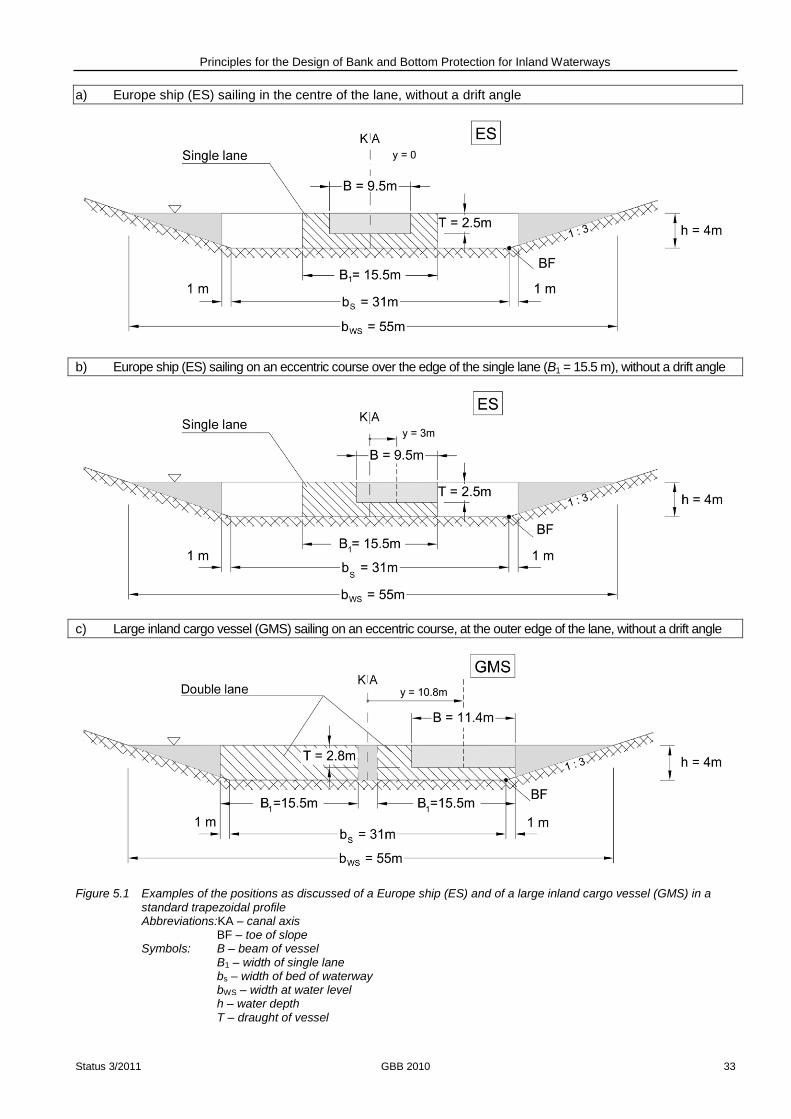
Principles for the Design of Bank and Bottom Protection for Inland Waterways
Status 3/2011 GBB 2010 33
a) Europe ship (ES) sailing in the centre of the lane, without a drift angle
b) Europe ship (ES) sailing on an eccentric course over the edge of the single lane (B1 = 15.5 m), without a drift angle
c) Large inland cargo vessel (GMS) sailing on an eccentric course, at the outer edge of the lane, without a drift angle
Figure 5.1 Examples of the positions as discussed of a Europe ship (ES) and of a large inland cargo vessel (GMS) in a standard trapezoidal profile Abbreviations:KA – canal axis
BF – toe of slope Symbols: B – beam of vessel
B1 – width of single lane bs – width of bed of waterway bWS – width at water level h – water depth T – draught of vessel

Principles for the Design of Bank and Bottom Protection for Inland Waterways
Status 3/2011 GBB 2010 34
5.5 Magnitude of ship-induced waves
(design situation: “sailing at normal speed”)
The primary wave field around a moving vessel is unevenly distributed. When the vessel is sailing in shallow water, the greatest return flow velocity occurs directly at the vessel and rapidly diminishes with increasing distance from it. This effect does not occur at the bank nearer to the vessel, when the latter is sailing close to a bank and the water is shallow. In this case, the drawdown and return flow velocity at the bank may even exceed those in the vicinity of the vessel. The return flow and drawdown caused by ships sailing on canals are distributed more or less uniformly.
The lack of uniformity of the return flow field is taken into consideration in the calculations by assuming that the entire return flow is concentrated in the influence width bE, i.e. occurs in an equivalent canal cross section, with the same values of the return flow speed as in the vicinity of the vessel. This enables the one-dimensional canal theory to be applied. The theory provides the drawdown and return flow velocity in the vicinity of the vessel and thus the critical ship speed.
Approximation equations are included in 5.5.1.1 to enable the cross-sectional area of this equivalent canal cross section to be determined as a function of the relevant influence parameters, which are the length of the vessel, the width of the canal and the distance of the vessel from the bank. The approximation equations are based on the 2-D potential theory for vessels being approached by a source-sink flow /BAW 2009/ (for derivation, see Annex D).
Approximation equations for the ratio of the drawdown at the bank to that at the vessel are also included in 5.5.1.1 on the basis of the same theory and depicted as a diagram in Figure 5.7. The ratio is taken into account when specifying the hydraulically equivalent slope inclination of the equivalent canal cross section approximated to a trapezoidal profile. This enables the mean water depth of this canal cross section to be calculated. The effective cross section of the vessel required for the application of the 1-D canal theory is determined in 5.5.1.2, taking account of the draughts at the bow and stern and the displacement effect of the boundary layer.
These data are used in 5.5.2 to calculate the critical ship speed. This forms the basis for the selection of the design ship speed, which is generally specified as a percentage of the critical ship speed. The mean drawdown and mean return flow velocity for this ship speed in the equivalent canal cross section and with a sailing line in the centre of the waterway are determined in 5.5.3. These are subsequently used to calculate the values at the bank, taking into account approximation equations given in 5.5.1.1 and depicted in diagram form in Figure 5.7. The drawdown and return flow velocity are then corrected in 5.5.4.3 to take account of the effects of the difference in the water levels between the bow and stern and the dynamic trim. This is necessary as the 1-D canal theory of potential flow used here does not allow for the difference in the water levels between bow and stern.
The continuity equation is used to calculate the maximum return flow velocity at the bank from the maximum local drawdown obtained above. Finally, the design wave heights at the bow and stern are determined (see 5.5.4.4). In doing so, the influence of the wave steepness and of shoaling effects on the wave heights has to be taken into account. This can be done by applying an empirical equation for the effect of the eccentricity of the sailing line /PIANC 1987a/.
The diagram in Figure 5.2 illustrates the entire procedure described so far.
Further aspects of the primary wave field are examined below in sections 5.5.4.5 to 5.5.4.8. These are the slope supply flow, influence of the drift angle, influence of the natural flow and drawdown velocity. Finally, section 5.5.5 deals with secondary waves, which generally occur independently of the primary wave field and can therefore be considered as independent load variables.
Particular hydraulic actions on canal linings, such as propeller jet, wind waves and other types of wave (positive surge/drawdown waves, flood waves) are considered in sections 5.6 to 5.7. In 7.1.3, the excess pore water pressures required for the geotechnical analyses are determined.

Principles for the Design of Bank and Bottom Protection for Inland Waterways
Status 3/2011 GBB 2010 35
Figure 5.2 Procedure for determining the hydraulic design parameters such as the maximum return flow velocity and maximum wave heights due to the primary wave field of ships sailing in shallow water when subject to shallow water and boundary layer effects, stating the relevant sections of this publication
5.5.1 Hydraulically effective cross section of canals and ships
5.5.1.1 Influence of shallow water
The area of the waterway cross section that is primarily involved in the drawdown and return flows and determines the equivalent canal cross section depends on the calculated width of the waterway.
br = A/h (5-1)
where
A is flow cross section, unmodified [m2]
h is water depth [m] see Figure 5.3
according to Figure 5.3, the effective influence width of the return flow field (bE) and the position of the vessel (eccentricity) within the cross section of the waterway. As a result, there are three width cases, which are illustrated in Figure 5.3. The differences between the width cases and the associated design principles apply to
ratios of water depth h to draught T where 1.25 h/T 5 /Kriebel 2003/ and of ship’s length L to beam B where
L/B 5.
For the practical application, it is advisable to use a sketch showing the dimensions of the cross section, influence width and position of the vessel in order to identify the case.

Principles for the Design of Bank and Bottom Protection for Inland Waterways
Status 3/2011 GBB 2010 36
Figure 5.3 Basic cases for the ratio of the influence width bE of the return flow field [see eq. (5-7)] to the calculated width br
of the waterway (approximative rectangular profile with the same cross section at the same water depth) [see eq. (5-1)]: A: canal: bE > br B: shallow water: bE < br C: transitional situation: bE includes one bank
Width case A: “Canal” long vessels, narrow canals
The return flow acts over the entire width of the canal when a ships’ hull is long in relation to the canal width. A canal cross section with the dimensions
bWS width of the canal at water level [m]
h depth of water [m]
m slope inclination [-] corresponding to the cotangent of the slope angle (tan = 1/m)
can therefore be used without modification for the following calculations based on the 1-D canal theory:
AK,äqui = AK (5-2)
AS,äqui = AS,eff (5-3)
mK,äqui = m (5-4)

Principles for the Design of Bank and Bottom Protection for Inland Waterways
Status 3/2011 GBB 2010 37
where
AK is the canal cross section [m2], AK = h (bWS - m h)
AK,äqui is the equivalent canal cross section [m2]
AS,äqui is the equivalent cross-sectional area of the ship [m2]
AS,eff is the effective cross-sectional area of the ship [m2], taking into account boundary layer effects and the
drift angle, where appropriate
mK,äqui is the equivalent slope inclination [-].
This situation, which applies only to canals, occurs when the greater distance ur,max (see Figure 5.4) between the axis of the ship and the imaginary bank of an approximative rectangular profile with the same area (R-profile) at the same depth of water, fulfils the following condition:
2E
maxr,
bu (5-5)
where
ur,max is the maximum distance to bank in the approximative rectangular profile [m] (see Figure 5.4) and
bE is the influence width of the return flow field [m].
Figure 5.4 Definition of the bank distances ur,min and ur, max to the bank lines of the approximative R-profile
For a trapezoidal profile featuring slopes with the same inclination, the following applies:
br = bWS - m h
ur,min = ½ br -y (5-6)
A = br h
The following approach applies to bE; it is dependent on the type of ship:
influence width bE of the return flow field [m]
)(2
BE BfLb
(5-7)

Principles for the Design of Bank and Bottom Protection for Inland Waterways
Status 3/2011 GBB 2010 38
where
B is the beam of the ship [m]
fB is the factor of the influence width [-], which is dependent on the type of ship
fB = 3 common inland navigation vessel
fB 1.5 modern seagoing vessel that can also navigate inland waterways, ship with bulbous bow
fB = 0 elliptical ship body plan (according to the theory)
L is the overall ship length [m].
The diagrams in Figure 5.6 and Figure 5.7 illustrating more precise calculations are based on equation (5-7) for fB = 3.
Equation (5-7) can also be applied in general cases, i.e. where fB ≠ 3, by substituting Leff / B for the ratio L / B in Figure 5.6 and Figure 5.7. The following applies to the effective ship’s length for slender ships:
effective ship's length Leff [m]
)3( Beff fBLL (5-8)
Slight shallow water effects may occur in canals and can be taken into account in the equivalent cross-sectional area for a more precise calculation in accordance with Figure 5.6, which has been derived from the simplified 2-D potential theory. The equivalent cross-sectional area of the canal AK,äqui is obtained as follows:
equivalent cross-sectional area of the canal AK,äqui
hbA äquir,äquiK, (5-9)
where
br,äqui is the calculated width of the equivalent canal cross section[m] and
h is the depth of water [m].
In canals, the change in the return flow velocity and drawdown between the ship and the bank is slight and can generally be disregarded. The following procedure can be followed for the transition from width case A to width cases B and C to achieve a more precise calculation:
The parameters determined using the equivalent cross-sectional area of the canal, i.e,
- mean drawdown h according to equation (5-24) in 5.5.3
- mean return flow velocity rückv in accordance with equation (5-23) in 5.5.3
decrease or increase between the ship and the bank (index ‘u’), resulting in new values (see eqs. [5-26] and [5-27]):
h uh
rückv urück,v
where
h is the mean drawdown averaged in the longitudinal and transverse directions [m]
uh is the mean drawdown averaged in a longitudinal direction at the bank [m]
rückv is the mean return flow velocity averaged in the longitudinal and transverse directions [m/s]
urück,v is the mean return flow velocity averaged in a longitudinal direction at the bank [m/s]
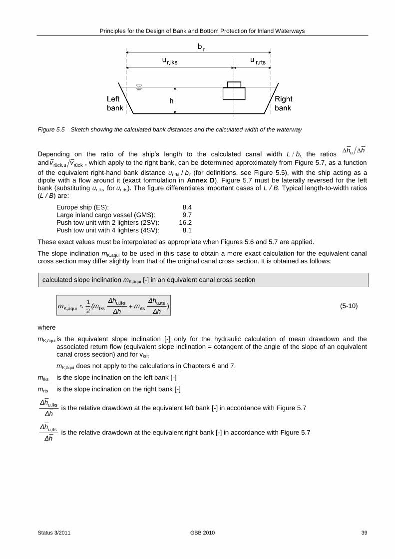
Principles for the Design of Bank and Bottom Protection for Inland Waterways
Status 3/2011 GBB 2010 39
Figure 5.5 Sketch showing the calculated bank distances and the calculated width of the waterway
Depending on the ratio of the ship’s length to the calculated canal width L br, the ratios hh u
and rückurück, vv , which apply to the right bank, can be determined approximately from Figure 5.7, as a function
of the equivalent right-hand bank distance ur,rts / b r (for definitions, see Figure 5.5), with the ship acting as a dipole with a flow around it (exact formulation in Annex D). Figure 5.7 must be laterally reversed for the left bank (substituting ur,lks for ur,rts). The figure differentiates important cases of L / B. Typical length-to-width ratios (L / B) are:
Europe ship (ES): 8.4 Large inland cargo vessel (GMS): 9.7 Push tow unit with 2 lighters (2SV): 16.2 Push tow unit with 4 lighters (4SV): 8.1
These exact values must be interpolated as appropriate when Figures 5.6 and 5.7 are applied.
The slope inclination mK,äqui to be used in this case to obtain a more exact calculation for the equivalent canal cross section may differ slightly from that of the original canal cross section. It is obtained as follows:
calculated slope inclination mK,äqui [-] in an equivalent canal cross section
)2
1 rtsu,
rts
lksu,
lksäquiK,hΔ
hΔm
hΔ
hΔ(mm (5-10)
where
mK,äqui is the equivalent slope inclination [-] only for the hydraulic calculation of mean drawdown and the associated return flow (equivalent slope inclination = cotangent of the angle of the slope of an equivalent canal cross section) and for vkrit
mK,äqui does not apply to the calculations in Chapters 6 and 7.
mlks is the slope inclination on the left bank [-]
mrts is the slope inclination on the right bank [-]
hΔ
hΔ lksu, is the relative drawdown at the equivalent left bank [-] in accordance with Figure 5.7
hΔ
hΔ rtsu, is the relative drawdown at the equivalent right bank [-] in accordance with Figure 5.7

Principles for the Design of Bank and Bottom Protection for Inland Waterways
Status 3/2011 GBB 2010 40
Figure 5.6 Calculated width of an equivalent canal cross section br,äqui as a function of the calculated canal width br
(see Figures 5.4 and 5.5 for definition) and the equivalent bank distances ur,rts and ur,lks for the right and left banks respectively (see Figure 5.5 for definition); ship’s length L and beam B for L / B = 5, 10 and 20
[for fB 3 in eq. (5-7), L is to be replaced by Leff according to eq. (5-8)].

Principles for the Design of Bank and Bottom Protection for Inland Waterways
Status 3/2011 GBB 2010 41
Figure 5.7 Mean return flow velocity ( rtsu,rück,v ) or drawdown ( rtsu,h ) at the equivalent (Index r) right (Index rts) bank
(Index u) in relation to the corresponding values at the ship ( hv ,rück ) and the bank distances ur,rts and ur,lks for
the equivalent right and left banks respectively (see Figure 5.5 for definitions); ship’s length L and beam B for L / B = 5, 10 and 20. N.B. Substitute ur,lks for ur,rts to calculate the values for the left bank (mirror image).

Principles for the Design of Bank and Bottom Protection for Inland Waterways
Status 3/2011 GBB 2010 42
The calculated trapezoidal profile, that is used as an equivalent in subsequent calculations then has the values AK,äqui, mK,äqui and h. The equivalent width at water level bWS,äqui can then be obtained from those values, i.e.
equivalent width at water level bWS,äqui [m]
hAhmb /äquiK,äquiK,äquiWS, (5-11)
where
AK,äqui is the equivalent canal cross section [m2] as per eq. (5-9) in 5.5.1.1
Note: If in the width case A all shallow water effects – such as the decrease of the return flow and drawdown fields towards the bank, as well as the resulting width of the equivalent canal cross section – are implemented according to Annex D, as in the Software GBBSoft /BAW 2008/, which corresponds to GBB 2010, the width cases B and C are thus also included. One exception is the approach for the shoaling of waves when the sailing line is eccentric (see 5.5.4.4). In this instance, the width case must be verified explicitly according to Figure 5.3.
Width case B: “Shallow water” short vessels, large bank distances
Shallow water conditions exist when a vessel is short in proportion to the width of the canal and for very large bank distances. This width case occurs when the smallest bank distance u r,min meets the following criterion according to Figure 5.4:
2
Eminr,
bu (5-12)
where
bE is the influence width according to eq. (5-7)
u r,min is the minimum bank distance in an equivalent canal cross section [m] (See Figure 5.4 for definition.)
The 1-D canal theory can then be applied by approximation to the following equivalent canal cross section AK,äqui, the width of which is limited by bE:
hbA EäquiK, (5-13)
For very large bank distances, that is, ur,min bE/2, the slope inclination of the equivalent canal cross section is
mK,äqui 0. In this case, the return flow velocity and the drawdown diminish towards the bank (distance ur) approximately as follows:
2
E
r
u
rück
urück,
1
1
b
uh
h
v
v
(5-14)
The much smaller decrease in the return flow field must be taken into account if a more exact calculation is required, particularly in the transition from width case B to width cases A or C. In this case, the following procedure should be followed:
- AK,äqui according to eq. (5-9)
- br,äqui according to Figure 5.6
- mK,äqui according to eq. (5-10)
- bWS,äqui according to eq. (5-11)
- Change h and rückv between the ship and the bank to the new values uh und urück,v according to
Figure 5.7.

Principles for the Design of Bank and Bottom Protection for Inland Waterways
Status 3/2011 GBB 2010 43
Width case C: “Transitional situation” Transition from canal to shallow water conditions
The influence width bE and the bank nearest the vessel overlap in the transitional area between canal and
shallow water conditions. The transitional area thus satisfies the following criterion:
maxr,E
minr,2
ub
u (5-15)
The equivalent canal cross section is obtained by approximation by disregarding the ineffective portion of the influence width bE (see Figure 5.3). The associated equivalent cross-sectional area AK,äqui is then:
hub
A
minr,
EäquiK,
2 (5-16)
The associated equivalent slope inclination is mK,äqui ≈ m / 2.
It can be assumed in the first approximation for the bank nearest the ship that rückurück, vv and hh u . For
a more exact calculation, see equations (5-9), (5-10) and (5-11) and Figure 5.6 and Figure 5.7.
5.5.1.2 Influence of boundary layers
As previously mentioned, the effects of boundary layers are taken into consideration. In this way, the energy losses at the hull of the ship that are disregarded in the 1-D canal theory can be quantified by approximation. This is done separately for the bow and stern regions by means of an effective cross-sectional area of the ship AS,eff in the prismatic section of the hull (midship section):
Bow (negligible boundary layer effects):
effective cross-sectional area of the ship at the bow AS,eff,B [m²]
BBBBS,Beff,S, TBAA (5-17)
where
AS,B is the cross-sectional area of the ship at the bow [m2]
BB is the beam at the bow [m]
TB is the draught of the ship at the bow [m]
B is the block coefficient of the cross-sectional area of the ship at the bow [-], usually B = 1.0
(prismatic midship section) N.B.: not to be confused with the block coefficient of the volume of the ship.
Stern (greatest boundary layer thickness):
effective cross-sectional area of the ship at the stern AS,eff,H [m²]
mm1HHS,Heff,S, 2TBAA
HHHS,H BTA (5-18)
5.2
SS
H10H1H log62.189.1645.0
K
LL

Principles for the Design of Bank and Bottom Protection for Inland Waterways
Status 3/2011 GBB 2010 44
where
AS,H is the cross-sectional area of the ship at the stern or at the point of greatest displacement [m2]
BH is the beam at the stern [m]
Bm is the mean beam between bow and stern [m]
KSS is the equivalent sand roughness of the ship’s hull [m], SSK ≈ m105.0103.0 33
LH is the development length of the boundary layer between the bow and the end of the midship section [m]
TH is the draught of the vessel at the stern [m]
Tm is the mean draught of the vessel between bow and stern [m]
H is the block coefficient of the ship cross section at the stern [-], generally equal to 1.0 (prismatic midship section) N.B.: not to be confused with the block coefficient of the volume of the ship.
1H is the thickness of the boundary layer at the stern [m] N.B.: It cannot exceed the dynamic underkeel clearance.
If the vessel does not have a prismatic hull, as is often the case with tugs, the cross section with the greatest displacement may be selected by way of an approximation of AS,eff. The thickness of the boundary layer will then need to be determined for that cross section.
5.5.2 Critical ship speed for canal conditions
In confined waterways with restricted depth and width, the flow around a ship and wave formation are subject to typical changes when the ship speed increases. While the water displaced by the ship flows in the opposite direction to the ship in the case of “subcritical” ship speed, when critical ship speed is reached, the unsteady development of the critical gradient required for the transition to supercritical flow begins.
An analysis of the results of field tests conducted with a modern large inland cargo vessel /BAW 2009/ in a canal (with approximately the standard trapezoidal profile in accordance with /BMV 1994/) indicates that calculations of the critical ship speed should include AK,äqui and AS,eff to account for the boundary layer around the ship’s hull and the shallow water effects described in 5.5.1. The tests /BAW 2009/, taking into account the unsteady course on approaching the bank, showed that the influence of eccentricity on the critical ship speed only proved to be significant for width case C in 5.5.1.1, that is, when ships that are short in proportion to the width of the canal sail close to the bank. The influence of eccentricity is taken into consideration below by reducing the width of the original canal cross section. The critical ship speed observed during the tests was slightly affected by the trim. Compared to vessels without a trim, ships with a static trim by the stern or a large stern-trim caused by the moving ship tend to decrease in critical ship speed and to increase in wave height.
Accordingly, the following equations apply to the mean drawdown at critical ship speed krith and the critical
ship speed vkrit (speed relative to the water) (Figure 5.8):
critical ship speed vkrit [m/s], associated mean drawdown krith [m]
mkritkrit hxh
(5-19)
mkritkrit ghyv
The values of xkrit and ykrit are calculated iteratively using the following auxiliary equations:
n
11
WS
m~
b
hmf
fxf~
1 krit
Principles for the Design of Bank and Bottom Protection for Inland Waterways
Status 3/2011 GBB 2010 45
(The value of xkrit (see below) must be provided here – the return address for iteration.)
)21(2* ff
f
3
1~*f
r
2/3
*2/1
krit ~2arccos
3
1
3cos~2~
r
frx
N.B.: Calculations in radian measure
f
xx krit
krit
~
N.B.: At this point return to calculation of f until the result is sufficiently stable.
2/1
2krit
kritkrit
1
2
fx
xy
The auxiliary functions are associated with the following parameters of the canal and the ship:
AK,äqui equivalent canal cross section [m2] as per eq. (5-9) in 5.5.1.1
AS,eff effective cross section of vessel [m2], allowing for boundary layer effects at bow and stern in accordance
with 5.5.1 and 5.5.4.6
b WS width at water level [m], b WS = b WS,äqui in accordance with eq. (5-11) in 5.5.1.1
hm mean water depth [m], hm = AK,äqui / b WS,äqui
m inclination of slope [-], m = mK,äqui in accordance with eq. (5-10) in 5.5.1.1
n blockage ratio [-], n = näqui =AK,äqui / AS,eff (equivalent blockage ratio)
In the iteration, the solution for a rectangular cross section can be used as an initial estimate for xkrit as follows:
arccos
3
1
3cos2kritx
N.B.: Calculations in radian measure
The dimensionless values ykrit for the critical ship speed and xkrit for the critical drawdown depend primarily on
the blockage ratio 1/n. The form parameter f~
, which describes the shape of the canal cross section, has a
slight effect on vkrit (see Figure 5.8). The influence of f~
on vkrit can be disregarded in rough calculations.
The value of vkrit for typical blockage ratios is then obtained from Figure 5.8. The influence of f~
on xkrit can be seen in Figures 5.8 and 5.11, from which approximate values can be determined.

Principles for the Design of Bank and Bottom Protection for Inland Waterways
Status 3/2011 GBB 2010 46
Figure 5.8 Dependence of the critical ship speed vkrit and the associated mean drawdown krith on näqui using the example
of a standard trapezoidal cross section (T-profile) and a standard rectangular cross section (R-profile)
Top diagram: 1 ≤ näqui ≤ 50 Bottom diagram: 1 ≤ näqui ≤ 4 (detail from top diagram)
Modified approaches, which may be consulted in /Römisch 1989/, among others, as an alternative to the approximation equation (5-19) given here, apply to the critical speed in special cases, such as waterway cross sections with a very irregular water depth (e.g. cross section with berms or dredged fairways).
A larger effective ship cross section must be used for vessels sailing with drift (see 5.5.4.7).

Principles for the Design of Bank and Bottom Protection for Inland Waterways
Status 3/2011 GBB 2010 47
5.5.3 Mean drawdown and return flow velocity for vessels sailing in the centre of a canal
The one-dimensional calculation of the return flow velocity and drawdown occurring when a vessel is in steady motion in a canal is based on Bernoulli’s equation (energy conservation) and the continuity equation (conservation of mass). The equations are applied to the undisturbed canal cross section in front of the vessel and the restricted cross section adjacent to the vessel caused by the submerged midship section and drawdown (see Figure 5.9). The canal cross section flows towards the hypothetical “fixed” vessel at the ship speed vs (relative to the water). In the literature, the symbol vSdW is also used for ship speed through water, however, in this document, only the symbol vS will be used throughout. It is assumed in this case that the flow distribution over the cross section is uniform, the squat of the vessel corresponds to the mean drawdown in the narrowest flow cross section (cross section with the greatest drawdown) using the simplified assumption: squat = drawdown, and any energy losses are disregarded. Furthermore, the dynamic trim of the vessel, if any, is not taken into consideration. With the exception of flow cross sections with rough beds and high levels of turbulence due to a superposed flow field, the 1-D canal theory provides reliable results, in spite of the simplifications referred to above, if the influences that are not taken into account are subsequently corrected empirically.
Allowance for boundary layer effects at the vessel and shallow water effects can be made to enable the application of the 1-D canal theory by approximation using the algorithms given in 5.5.1 with an equivalent cross-sectional area of the canal AK,äqui and an effective cross-sectional area of the ship AS,eff. The influence of a natural current on the calculation of the drawdown for a specified ship speed over ground vSüG is taken into account by calculating the ship speed through water vS:
Ship speed through water vS[m/s]
StrSüGS vvv (5-20)
(+: upstream travel, -: downstream travel)
where
vStr is the mean flow velocity [m/s] in the cross section
vSüG is the ship speed over ground [m/s]
If vS = 0.97vkrit is assumed for design purposes, this corresponds to the ship speed through water. The flow
velocity is then irrelevant to the calculation of the drawdown. Accordingly, each of the speeds given below is measured in relation to the surrounding body of water. The effect of the natural flow close to the bank must be considered when determining the required size of armour stones, as it will determine either an increase or a decrease in the size, see 5.5.4.6.
Figure 5.9 Sketch showing how to calculate the flow due to displacement; see text and eqs. (5-21) to (5-23) for explanation of (some of the) symbols
The following two basic relationships then apply:
1. The maximum drawdown h in the narrowest flow cross section adjacent to the ship, averaged over the width of the canal, is obtained by means of Bernouilli’s equation (Figure 5.9):
2
S
2
rückS1x2
1vvv
ghhh (5-21)

Principles for the Design of Bank and Bottom Protection for Inland Waterways
Status 3/2011 GBB 2010 48
2. In accordance with the continuity equation
rückmM vvhbAAvA SS (5-22)
the associated return flow velocity at the bow and stern, averaged over the cross section, is:
return flow velocity averaged over the cross section rückv [m/s]
SS
mM
mMrück
)(v
AA
Av
hbAA
hbAv
(5-23)
where
A is the canal cross section [m2], A = A
K,äqui as defined in 5.5.1.1
AM is the submerged midship section (making allowance for boundary layer effects and shallow water effects at bow and stern) [m
2], AM = AS,eff according to 5.5.1.2 and 5.5.4.7
ΔA is the reduction in the cross section of the canal due to the cross section of the ship and drawdown [m2],
hbAA mM
bm is the mean width at water level in the drawdown area [m], mhbb WSm
bS is the width of the bed [m]
bWS is the width at water level [m], äquiWS,WS bb according to eq. (5-11) in 5.5.1.1
g is the acceleration due to gravity [m/s²]
h is the depth of water in the canal [m]
hx is the depth of water at the narrowest flow cross section [m]
h is the maximum drawdown in the narrowest flow cross section, averaged over the width of the canal [m]
m is the slope inclination [-], m = mK,äqui in accordance with eq. (5-10) in 5.5.1.1
T is the draught of ship at the midship section [m]
vS is the ship speed through water [m/s] according to eq. (5-20)
rückv is the mean return flow velocity [m/s],
Note: relative to an observer moving at vStr
1 is the correction coefficient [-] according to eq. (5-25)
The implicit method of calculating the relationship )( Svfh is derived from eq. (5-21):
correlation between ship speed through water vS [m/s] and mean drawdown h [m]
1
22
1
S
AA
A
hgv
(5-24)
Principles for the Design of Bank and Bottom Protection for Inland Waterways
Status 3/2011 GBB 2010 49
where
1 is the correction coefficient [-] according to eq. (5-25)
The solution of this calculation method is performed iteratively after specifying h (normal range between 0.2 and 0.5 m) until the calculated speed corresponds to the design ship speed. Plotting the calculated ship speed
through water vS against h is recommended (see Figure 5.10). rückv can then be calculated using eq. (5-23).
The correction coefficient 1 used in eqs. (5-21) and (5-24), which describes, amongst other things, the
influence of the irregularity of the return flow field depending on how close the actual ship speed is to the critical ship speed, is stated by /Przedwodjski et al. 1995/:
krit
S1 4.04.1
v
v (5-25)
For small vs/v
krit ratios, the correction coefficient
1 leads to drawdown h occurring, even where the n ratio
(reciprocal value of the blockage ratio) is very large and also in the theoretical special case n
(very flat bank slopes), that is, when no more mean return flow can actually exist. This is because of the local flow around the ship that also occurs in deep water without significant displacement effects. This localised flow field depends mainly on the contours of the ship and declines rapidly with increasing distance from the ship. Calculation results which were arrived at in the equations (5-21) to (5-24) using eq. (5-25) for slender ship contours, large distances from the bank or low ship speeds, are therefore often well on the safe side.
An exact calculation in accordance with eq. (5-24) is not necessary if only a rough estimate is required. Instead,
calculations can be performed with vS / vkrit, the blockage ratio 1/n, form parameter f~
and Figure 5.11.
The values of the return flow velocity rückv and drawdown h must be multiplied by the ratios given in 5.5.1.1,
Figure 5.7, to allow for their decline between the ship and the bank and to obtain the corresponding values at
the bank urück,v and uh :
5.7Figure
uu
h
hhh (5-26)
5.7Figurerück
urück,
rückurück,
v
vvv (5-27)
h and rückv are design values for ships sailing in the centre of the waterway. They serve as input data for
other empirical calculations regarding the influence of the water surface gradient and eccentric sailing lines according to 5.5.4.2 to 5.5.4.4.
Numerous other calculation methods have been developed for the 1-D canal theory /Bouwmeester 1977/;
/Dand, White 1978/; /Führböter et al. 1983/; /Jansen, Schijf 1953/; /Söhngen 1992/. The mean drawdown h provided by each of the methods referred to here is a value obtained by averaging over the primary wave only.

Principles for the Design of Bank and Bottom Protection for Inland Waterways
Status 3/2011 GBB 2010 50
Figure 5.10 Ship speed through water vs calculated with eq. (5-24) as a function of the mean drawdown h in accordance with the 1-D canal theory for a large inland cargo vessel (length L = 110 m , beam B = 11.4 m, draught
T 2.8 m, thickness of boundary layer at bow section 1H = 0.19 m) in standard trapezoidal and rectangular
profiles
Symbols: R - rectangular, T - trapezoidal

Principles for the Design of Bank and Bottom Protection for Inland Waterways
Status 3/2011 GBB 2010 51
Figure 5.11 Relative values (in relation to krith and mh ) of the mean drawdown h as a function of näqui and the form
parameter f~
for typical relative ship speeds vS / vkrit calculated using the 1-D canal theory. (The calculations
were based on the sailing line in the centre of the canal for a large inland cargo vessel with a draught of 2.8 metres and a kSS of 0.4 mm).

Principles for the Design of Bank and Bottom Protection for Inland Waterways
Status 3/2011 GBB 2010 52
5.5.4 Hydraulic design parameters and geotechnically relevant drawdown parameters for
any sailing position
5.5.4.1 Definition of wave height
The design ship-induced wave heights H at the bow (HB) and stern (HH) are calculated taking account of the
calculated canal width at the centre of the slope. Any changes in the waves running up the slope are not dealt with separately but are incorporated into the overall design calculations.
The basic primary and secondary wave patterns, as they would be perceived by a stationary observer on the bank, are shown in Figure 5.12.
Figure 5.12 Formation of ship-induced primary waves at subcritical (vS < vkrit), critical (vS vkrit) and supercritical (vS > vkrit) speeds
5.5.4.2 Maximum drawdown at bow and associated return flow velocity without the
influence of eccentricity
The cross section of the vessel at the bow must be used to calculate the maximum drawdown at the bow, allowing, where applicable, for boundary layer and shallow water effects as described in 5.5.1. The following equation /Przedwojski et al. 1995/ applies to the height of bow waves at the bank for modern large inland cargo vessels and tugs, when there is no influence of eccentricity; the equation takes account of, amongst other things, the water level elevation ΔhWA,B in front of the bow:
maximum drawdown near the bank at the bow u,Bugh [m] without the influence of eccentricity
Bugu,1Bugu,ˆ hFh (5-28)
where
F1 is the factor for the maximum water level drawdown in proximity to the bank at the bow of the vessel [-] standard: F1 = 1.1 recreational craft F1 = 1.0
Note: The coefficient may be greater than 1.1 for a full bow.
Bugu,h is the maximum water level drawdown near the bank at the bow [m]
u,Bugh is the mean water level drawdown near the bank at the bow [m], calculated for the blockage ratios at the
bow according to 5.5.3

Principles for the Design of Bank and Bottom Protection for Inland Waterways
Status 3/2011 GBB 2010 53
The influence of eccentricity on the bow wave is taken into account in 5.5.4.4.
The maximum return flow velocity at the bow Bugu,rück,v can be calculated approximately from the continuity
equation eq. (5-23) when, in this equation, Bugu,h is substituted for h . It should be borne in mind that both bm
and A are affected by Bugu,h
5.5.4.3 Maxium drawdown at the stern and associated return flow velocity without the
influence of eccentricity
The difference between the maximum drawdown at the stern and uh [see eq. (5-26)] depends on the following
influences:
(1) Ratio of draught to water depth. (The ratio Hecku,Hecku, /ˆ hh tends to be greater for smaller hT / ratios.)
(2) Type of propulsion ( Hecku,h tends to be greater for twin-screw vessels sailing close to a bank than for
single-screw vessels.)
(3) Closeness to vkrit (due to the increase in the water surface gradient between the bow and the stern, the associated stern-heavy trim and the secondary waves caused by the transverse stern wave as described in 5.5.5)
(4) Superposition of secondary waves originating at the bow for short vessels or wide canals (distance case B as described in 5.5.5.1)
Influences (1) and (3) can be taken into consideration approximately by means of the following equation according to the approach of /Przedwojski et al. 1995/:
maximum drawdown near the bank at the stern u,Heckh [m] without the influence of eccentricity
u,HeckHHeck,uˆ hCh (5-29)
where
CH is the factor for the influence of the type of ship, draught, trim and water level difference between bow and stern [-]
CH ≈ 1.3 for modern inland navigation vessels (T / h ≈ 0.7)
CH ≈ 1.5 for partially laden, in particular ballasted, modern inland navigation vessels and tugs (T / h ≈ 0.4)
CH ≈ 1.1 for sea-going vessels that can also navigate inland waterways, as they usually have a large bow trim
Hecku,h is the mean drawdown near the bank [m], calculated according to 5.5.3 for the blockage ratios at the
stern.
Heck,uh is the maximum water level drawdown near the bank at the stern [m]
Additional transverse stern waves may occur at ship speeds close to vkrit; they are described in 5.5.5.3. They
may affect u,Heckh to a greater extent than the influences (1) - (3) described above, in particular if the
additional influence (4) occurs.
As an alternative to eq. (5-29), Heck,uh results from the following equation, in accordance with measurements of
the BAW at the Wesel-Datteln Canal /BAW 2009/:
qSek,Hecku, H2
1hΔˆ h (5-30)

Principles for the Design of Bank and Bottom Protection for Inland Waterways
Status 3/2011 GBB 2010 54
where
HSek,q is the height of the additional secondary wave according to 5.5.5.2 from eq. (5-61), also taking account of eq. (5-65).
If influence (4) occurs, the part of the height of the secondary bow wave below the still-water level (SWL),
obtained by means of eq. (5-56) (see 5.5.5.2) must be added to u,Heckh in accordance with eq (5-29) or
eq. (5-30).
The maximum return flow speed at the stern Hecku,rück,v can be calculated approximately from the continuity
equation eq. (5-23) when, in this equation, Hecku,h is substituted for h . It should be borne in mind that both bm
and A are affected by Hecku,h .
5.5.4.4 Maximum heights of bow and stern waves due to eccentric sailing
There is a steep increase in the wave heights at the slope as the distance between the vessel and the banks decreases. This is because, as the bank distance decreases, wave lengths continually decrease, given a constant wave energy level, and increasing wave heights are associated with these. The increase in wave height at the bank nearest the ship is calculated as follows as described by /Przedowojski et al. 1995/ as a function of the ratio of the cross-sectional area between the ship and the bank to the canal cross section (or, for vessels sailing in shallow water, to the equivalent cross-sectional area of the canal in accordance with 5.5.1.1); see Figure 5.13:
Figure 5.13 Definition of A' for eccentric sailing in width case A in accordance with 5.5.1.1
maximum bow wave height Hu,Bug [m] at the bank closer to the vessel for eccentric sailing
Bugu,Bugu,ˆ)
'20.2( h
A
AH (5-31)
maximum stern wave height Hu,Heck [m] at the bank closer to the vessel for eccentric sailing
Hecku,Hecku,ˆ)
'20.2( h
A
AH (5-32)
where
A is the relevant cross-sectional area of the canal [m2]
A' is the cross-sectional area between the ship’s axis and the bank [m2] (see Figure 5.13)
A'/A is the ratio [-] corresponding to the cases described in 5.5.1.1 and Figure 5.3
To determine A’/A, the following equations – depending on the width case – are recommended:
Principles for the Design of Bank and Bottom Protection for Inland Waterways
Status 3/2011 GBB 2010 55
Width case A: 0br
minr,
u
A
A (5-33)
Width case B: 5.0
A
A (5-34)
Width case C: 0
2minr,
E
minr,
ub
u
A
A (5-35)
u,Bugh is the maximum drawdown near the bank at the bow [m] according to 5.5.4.2
u,Heckh is the maximum drawdown near the bank at the stern [m] according to 5.5.4.3
The above mentioned conditional equations for A’/A can stand without a direct interpretation of the cross sections by hypothesis of ur,min and bE. Alternatively to these conditional equations, A’ and A could be calculated from the equivalent canal cross section. To do so, however, the cross section of this eccentricity would have to be verified; this eccentricity may deviate from that in the original profile, and no conditional equations for it are stated here. Therefore the above mentioned equations are also used in the software GBBSoft. In this, only the width case according to Figure 5.3 is to be identified, even if br,äqui is determined in width case A with the more precise methods.
If a vessel is sailing extremely close to a bank, the point of impact of the interferences caused by the diverging waves of the secondary bow wave system may coincide with the maximum drawdown at the stern. In this case, half the height of the secondary wave HSek according to eq. (5-56) must be added to the height of the stern wave according to eq. (5-53), which is used for armour stone dimensioning, but not for geotechnical design (special instance of distance case B in 5.5.5.1).
Hu,Bug and Hu,Heck can be taken as u,Bugh and u,Heckh respectively at the bank furthest from the vessel for
design purposes.
The influence of the proximity to the bank on the return flow velocity is small and can be disregarded. The design values are therefore obtained directly, as described in 5.5.4.2 and 5.5.4.3
5.5.4.5 Slope supply flow
A significant slope supply flow parallel to the bank occurs when stern waves break, but also in the case of high stern waves that do not break, and when a vessel sails close to the bank. It is indicated by the area of spume travelling alongside the vessel (Figure 5.14).
The flow velocity umax relative to the moving vessel which occurs at the height of the revetment stones, without allowing for a natural flow velocity close to the bank, reaches the same velocity as the ship, if the waves are very high, or if they break, plus the turbulent fluctuations. In the case of lower wave heights, the flow velocity depends above all on the ratio of the ship speed to the celerity of the breaking wave calculated by: local water
depth ≈ wave height (parameter rF~
). The following approximation equation for umax has been derived from measurement data of the BAW (German Federal Waterways Engineering and Research Institute) for the Wesel-Datteln Canal /BAW 2009/:
maximum velocity of slope supply flow umax [m/s]
smax 3.0 vu for 83.1~ 2 rF
svrF
vu
12.1
71.0~
17.03.02
smax (5–36)
for 83.1~
71.0 2 rF
smax 0.1 vu for 71.0~ 2 rF

Principles for the Design of Bank and Bottom Protection for Inland Waterways
Status 3/2011 GBB 2010 56
Figure 5.14 Slope supply flow for vessels sailing close to a bank. The photos show a laden inland cargo vessel (GMS) (top), an empty inland cargo vessel (GMS) (centre) and a tug boat (bottom) in a standard trapezoidal profile (T-profile)

Principles for the Design of Bank and Bottom Protection for Inland Waterways
Status 3/2011 GBB 2010 57
where
rF~
is the Froude number formed using the maximum height of the stern waves instead of the water depth
Hecku,
2
S~
Hg
vrF
(5-37)
Hu,Heck is the maximum height of the stern waves [m] according to 5.5.4.4, eq. (5-32) (design wave height)
vS is the ship speed through water [m/s]
umax is the maximum velocity of the slope supply flow at the height of the revetment stones [m/s]
An approach in which the roughness of the slope revetment is taken into consideration has been described by /Verhey, Bogaerts 1989/.
In addition to the parameter rF~
, the local Froude number and the ratio of the wave height Hu,Heck to the distance
from the bank ueff determine whether a significant slope supply flow will occur or not. Sailing tests carried out on
the Wesel-Datteln Canal /BAW 2009/ have enabled the definition of the areas shown in Figure 5.15 (breaker criterion). The Froude number is obtained from the maximum return flow velocity and maximum wave height at the stern in accordance with 5.5.4.3 and 5.5.4.4.
According to current experience the above mentioned eq. (5-36) and the breaker criterion according to Figure 5.15 apply only to canals with typical blockage ratios where n lies approximately between 5 and 10. For large n ratios and large bank distances, umax is generally overestimated when using eq. (5-36). This is particularly true for low ship speeds, where the lower threshold value 0.3 vS is decisive as, strictly speaking, the factor 0.3 decreases as n increases.
New studies have shown that umax should only be used for design purposes when the breaker criterion has been
met, as only breaking waves have a severe erosive impact on armour stones. A calculation method on this basis has been developed by /Söhngen et al. 2010/. It is particularly recommended for large bank distances for which eq. (5-36) tends to produce values that are too high.
Figure 5.15 Distinction between unbroken waves, waves with significant slope supply flow and waves that have fully broken at slopes for vessels sailing close to the bank (breaker criterion)

Principles for the Design of Bank and Bottom Protection for Inland Waterways
Status 3/2011 GBB 2010 58
5.5.4.6 Determining the critical flow velocities close to the bank where a natural current
is present
The equations shown in 5.5.3 and 5.5.4.5 use the ship speed through water vSdW for calculating the ship-induced flows parallel to the slope. If the inland navigation vessel is in a waterway with a natural current, this means that the calculated flow speeds must be regarded as relative to an observer moving at vStr. In order to obtain the values relative to the bank that are relevant for dimensioning the size of the armour stones, the influence of the natural flow must also be allowed for in retrospect. Corresponding to the differing flow directions of the return flow and the slope supply flow and the direction of motion upstream or downstream, the natural flow may have the effect of reducing or increasing the values as the case may be.
For the flow velocity, the value vstr,Ufer for a sailing line close to the bank must be assumed, as the revetment is situated at the bank. This will be less than the mean flow velocity. If no measurement data is available, the following approximation for the mean flow velocity without influence of shipping in the vicinity of the slope can be made assuming the flow velocity distribution according to Gauckler-Manning-Strickler:
3
2
v
Str
uStr,StrUferStr,
hk
kvv
(5-38)
where
h is the water depth [m] in the trapezoidal cross section
kStr,u is the Strickler roughness [m1/3
/s] of the bank, i.e. of the revetment ( 30 m1/3
/s)
kStr is the mean Strickler roughness [m1/3
/s] of the lateral cross section (from hydraulic calculation)
vStr is the mean flow velocity [m/s] in the cross section
v is the boundary layer thickness [m] of the return flow field (estimated value 1 m)
For the maximum flow velocity vmax in the vicinity of the bank consisting of return flow and flow velocity, as it is to be used in eq. (6-10) for the dimensioning of armour stones, the following values result:
with flow velocity in the direction of motion (downstream motion):
Ufer,Strrückmax vvv (5-39)
with flow velocity against direction of motion (upstream motion):
Ufer,Strrückmax vvv (5-40)
where
vmax is the maximum flow velocity [m/s] made up of return flow and flow velocity vStr,Ufer in the vicinity of the bank (at a distance equal to the thickness of the boundary layer of the return flow field)
rückv is the maximum return flow velocity [m/s]
rückv = Bugu,,rückv
for the bow region according to 5.5.4.2
rückv = Hecku,,rückv
for the stern region according to 5.5.4.3
vStr,Ufer is the mean flow velocity [m/s] without influence of navigation close to the slope according to eq. (5-38)
The same considerations apply for the load on the slope caused by the slope supply flow as for the return flow velocity. Here, the effect of the natural flow, however, acts exactly counter to that of the return flow. Because the slope supply flow runs with the ship in the direction of motion of the vessel, the speed of the slope supply flow increases by the magnitude of the natural flow at the bank, when a vessel is travelling downstream and the ship is therefore travelling in the direction of flow. This provides the design speed for the slope supply flow umax,B that is to be used in eq. (6-11):

Principles for the Design of Bank and Bottom Protection for Inland Waterways
Status 3/2011 GBB 2010 59
with flow velocity in the direction of motion (downstream motion):
UferStrB vuu ,maxmax, (5-41)
with flow velocity against direction of motion (upstream motion):
UferStrB vuu ,maxmax, (5-42)
where
umax,B is the design speed in the slope supply flow [m/s]
umax is the maximum velocity of slope supply flow according to 5.5.4.5
vStr,Ufer is the mean flow velocity [m/s] without influence of navigation close to the slope according to eq. (5-38)
5.5.4.7 Increase in wave heights in the case of vessels sailing with drift
Even when a vessel is sailing along a straight stretch, a drift angle D can occur temporarily between the axis of the ship and that of the canal as a result of the meandering course of the vessel; according to /BMV 1994/ it is to be estimated at approx. 2.1° (for large inland cargo vessels GMS) or approx. 1.25° (for 185-metre push tow units); see Figure 5.16.
The drift angle D is considerably larger when a vessel navigates a bend (see Figure 5.16b), particularly for
older vessels and for vessels not using a bow rudder. It can be obtained from the relative position of the ship’s pivot point (tactical centre of rotation determined by the dynamic constant cF) in accordance with Figure 5.16b.
In still water, design tasks for navigational dynamics should take the values cF 0.9 for push tow units and
cF 1.0 for large inland cargo vessels, as recommended by /Dettmann 1998/. The guidelines in the Netherlands
/RVW 2009/ recommend values of cF 0.7 for fully laden ships and cF 1.0 for empty vessels. Reference
should be made to /Dettmann, Jurisch 2001/ and /Söhngen, Tittizer 2009/ regarding the influence of flow.
This effect of the drift angle is taken into account by defining a notionally enlarged submerged midship section AS, eff,D (boundary layer effects being disregarded).
ship cross section AS,eff,D of a ship sailing with drift [m²]
MD
Deff,S,
sin25.0A
B
)β L (BA
(5-43)
where
AM is the submerged midship section [m²] (the boundary layer is disregarded here)
B is the beam of the ship [m]
L is the length of the ship [m]
D is the drift angle [°]
The changes in the loads on the slope that occur when a ship sails with a drift angle are introduced into the design by means of AS,eff,D (instead of AS,eff according to 5.5.1.2) and the eccentricity of the vessel, which may be increased, if appropriate (a critical factor for the dimensioning of the armour stones is, as a rule, the position of the stern of the vessel, more precisely, the position of the ship section at the stern) (because AS,eff,D > AM). The influence of the drift angle on the hydraulic design parameters is small for vessels sailing alone and is only relevant for long push-tow units. Both cases may need to be considered, as it is not possible to decide in advance whether sailing with or without drift will be relevant to the design.

Principles for the Design of Bank and Bottom Protection for Inland Waterways
Status 3/2011 GBB 2010 60
Figure 5.16 Diagram showing how to determine the drift angle on straight stretches (a) and on bends (b)
As the calculation methods offered in GBBSoft only assume a position of the ship parallel to the bank, several ship positions may have to be examined (see Figure 5.17). This is because the ship positions have differing effects on the various design target parameters:
- As already stated above, the eccentricity of the ship’s position in the cross section corresponding to the position of a ship section close to the stern (generally identical with the position of the draught mark farthest aft, about LH in distance from the bow) should be selected for the dimensioning of armour stone size from slope supply flow.
- On the other hand, the position of the ship’s bow that is closer to the bank, or rather, of the beginning of the midship section (generally positioned at the first draught mark – at a distance of about LB from the bow) can be decisive for the geotechnical design. Corresponding to this smaller distance from the bank, a greater eccentricity of the ship’s course from the axis is to be assumed. So that the stern does not determine the drawdown time – which can indeed be the case, when calculating, for ships with ballast – the stern draught should be reduced in the calculation.
- Should the return flow velocity be relevant to the design, then both the bow (because it is closer to the bank) and the stern (for example, because it is ballasted) may require larger design values.
In order to cover all the above special cases, it is advisable, in the case of motion at a significant angle of drift, to distinguish between the three situations described below. For simple, practical calculations, the consideration of the ship in a centred position is fully adequate.
Figure 5.17 Sketch showing the three situations recommended for the design in the event of a sailing line with a significant angle of drift

Principles for the Design of Bank and Bottom Protection for Inland Waterways
Status 3/2011 GBB 2010 61
1. Ship position close to bank (N.B.: when the inner bank of the bend is the design bank)
The position close to the bank corresponds to the position of the beginning of the midship section in the area of the bow of the ship. For the dimensioning of the armour stones from the return flow at the bow, and for the geotechnical design from the drawdown time and drawdown at the bow, the draught at the stern is reduced in the calculation. If the bow position is known, for example, from a particular alignment using rectangular ship symbols, the additional distance of the midship section from the bank will be calculated as follows:
DBLu sin (5-44)
where
∆u is the additional proportion of the bank at the bow of the ship (see Figure 5.17)
LB is the distance of the bow from the beginning of the midship section
LB 0.1 – 0.2 ship lengths
D is the drift angle [°]
2. Ship position farthest from bank (N.B.: when the inner bank of the bend is the design bank)
The position farthest from the bank corresponds to the position of the end of the midship section at the stern of the ship. This is decisive for the sizing of the armour stones based on return flow, slope supply flow and wave height at the stern. If the bow position is also known in this case, the midship section lies additionally at the following distance from the bank:
DHLu sin (5-45)
where
LH is the distance of the bow from the end of the midship section
3. Position of the centre of the ship
As a first approximation for all design sizes for unmodified draughts, the position of the centre of the ship relative to the bank can be used. The relevant bank distance in comparison with that of the bow is then:
D
BH LLu sin
2
(5-46)
where
(LH+LB) /2 is the distance of the bow from the centre of the ship (if LH and LB are unknown, L / 2 may be taken as an approximation)
5.5.4.8 Drawdown from ship-induced waves
A moving vessel will cause the water to flow around it, giving rise to bow swell, drawdown and a stern wave owing to the localised and temporary changes in the blockage ratios. The maximum drawdown values za,B and za,H at the bank (based on the elevated water level caused ahead of the ship at any given moment, without the bow wave height as a result of the bow swell), the associated drawdown time ta and, thus, the drawdown speed
zav must be known for geotechnical design considerations (see. 7.1).

Principles for the Design of Bank and Bottom Protection for Inland Waterways
Status 3/2011 GBB 2010 62
Figure 5.18 Basic correlation between drawdown za,B or za,H [eqs.(7-1) and (7-2)] and drawdown time ta for the geotechnical design
In general, the following approximation equation applies for small bank distances
(“small bank distance” = up to bE/2) for the time ta,B of the maximum drawdown at the bow
(including water surface elevation ahead of the bow: za,B according to Figure 5.18):
SüG
effa,B
v
uCt (5-47)
where
C is a constant [-] C = 1.7 for large and extra-large inland cargo vessels C = 1.5 for tugs C = 1.3 for relatively old vessels with a full form, e.g. Europe ship and pushing units
ta,B is the drawdown time at the bow [s] (see Figure 5.18)
ueff is the effective bank distance [m] (distance between the ship’s axis and the equivalent bank line at still-water level as shown in Figure 5.19) N.B.: The equivalent bank line is situated in the centre of the remaining slope on the bank nearest the ship.
vSüG is the ship speed over ground [m/s], which is linked with the ship speed through water vS and the flow velocity vStr according to eq. (5-20).
Figure 5.19 Definition of effective bank distance ueff (distance between ship’s axis and equivalent bank line) in a symmetrical trapezoidal profile

Principles for the Design of Bank and Bottom Protection for Inland Waterways
Status 3/2011 GBB 2010 63
The following equations apply to the effective bank distance in symmetrical trapezoidal profiles, depending on the position of the vessel (for definitions, see Figure 5.19):
Ship passes over the toe of the slope :
22
rtsr,
hmBu
442
rtsr,eff
Bhmuu (5-48)
N.B.: The bilge line of the ship must not pass over the slope.
The ship maintains a larger distance to the bank (i.e. not above the slope):
22
rtsr,
hmBu r,rtseff uu (5-49)
The drawdown time, even when a vessel is sailing extremely close to a bank, cannot be arbitrarily small, as in this case the reduction is limited by the secondary wave system.
For 8.0mS ghv the smallest possible drawdown time applies:
Seka,B,a,B tt (5-50)
where
ta,B is the drawdown time at the bow in general [s]
ta,B,Sek is the drawdown time of the maximum secondary bow wave [s] in accordance with eq. (5-51)
The drawdown time of the secondary bow waves is calculated – distinguishing between transversal and diverging waves – as follows:
SüG
2S
Seka,B,vg
vt for transversal waves
(5-51)
SüG
2S
Seka,B,3
2
vg
vt for diverging waves
The maximum of both values calculated with eq. (5-51), that is the drawdown time of the transversal waves at the bow, is used in eq. (5-50). The values determined using eq. (5-51) are also to be used for the special case of secondary wave load only, for example, from recreational craft.
The stern wave system predominates in the case of vessels with static trim at the stern, for instance during empty runs (runs with ballast) and small, relatively fast craft, a tug or recreational craft. For the drawdown time at the stern ta,H the following applies:
SüG
pris
a,Ba,Hv
Ltt (5-52)
where
prisL is the length of the hull with a largely prismatic cross section [m]
LL 9.0pris for push tow units with 2 lighters (2SV)
LL 8.0pris for large inland cargo vessels (GMS) and Europe ships (ES)
LL 3.0pris for recreational craft with transom stern
LL 0.0pris for tugs
The average drawdown velocity zav is obtained by dividing the relevant wave height by the associated
drawdown time.

Principles for the Design of Bank and Bottom Protection for Inland Waterways
Status 3/2011 GBB 2010 64
5.5.5 Secondary waves
5.5.5.1 General remarks
All the equations shown in 5.5.5.2 and 5.5.5.3 apply only up to the planing speed of the ship according to eq (5-69) in 5.5.5.4, Up to this speed, the secondary wave heights increase. For greater ship speeds they decrease again. For this special case an approximation equation for recreational craft is shown in 5.5.5.4.
Vessels in motion generate diverging and transversal waves that originate at the bow and stern (Figure 5.20). It is these waves that form the secondary wave system. The waves are superposed on each other and form pronounced interference lines at which the highest waves occur.
For Froude numbers based on depth ghvFr Sh up to 0.7, or up to 0.8 for rough estimates, the interference
line is inclined towards the ship’s axis at the Kelvin angle K of approx. 19°. The fronts of the diverging waves
are inclined at an angle W ≈ 55° in relation to the ship’s axis and, thus, also in relation to the canal bank when the ship is sailing approximately parallel to the bank. The angle of impact of the diverging waves will be modified if the ship is not sailing parallel to the bank, and this must be taken into consideration in the following equations.
Figure 5.20 Secondary wave system for 8.0h Fr
The secondary waves diverge as they travel towards the bank, decreasing in height in the process. The scaling parameter is the distance to the bank u, which, unlike the methods for the primary wave system, is always measured at the height of the (approximated) still water level when calculating the secondary wave heights. Transversal waves diminish to a greater extent than diverging waves. The three design cases described below must generally be taken into account, as the transversal waves of the stern wave system are more pronounced than those of the bow wave system, particularly for short, fast ships and vessels on empty runs, although the diverging bow waves are larger than the diverging stern waves (see Figure 5.21).
The drawdown due to the return flow field may need to be taken into account in the case of high values of h
when determining u or u '. In this case, u and u ' are reduced by around m uh
( uh in accordance with eq. (5-26) in 5.5.3).

Principles for the Design of Bank and Bottom Protection for Inland Waterways
Status 3/2011 GBB 2010 65
Figure 5.21 Standard distance cases for secondary waves
Distance case A
The primary and secondary wave systems are not usually superposed on each other in a way that is relevant to
the design where u ' < L tanK, i.e. when they are generated by vessels that are long in relation to the width of the canal or for short bank distances (the standard situation for Europe ships (ES), large inland cargo vessels (GMS) and push tow units (SV) in canals). The heights of the secondary waves are obtained as described in 5.5.5.2. The armour stone size required for stabilisation of the slope can therefore be calculated separately for the primary and secondary wave fields (cf. 6.2 and 6.4).
Further information regarding the distance cases:
The calculation of distance case A using precise calculation methods includes the distance cases B and C.

Principles for the Design of Bank and Bottom Protection for Inland Waterways
Status 3/2011 GBB 2010 66
Distance case B
The transversal stern wave of the primary wave system may be superposed on the interferences of the
secondary bow waves in wide canals or in the case of short vessels. This is approximately valid for u’ = L tanK.
Since because of their length the waves are not always superposed at precisely the distances stated above, it is advisable to define a distance range u’ü instead of the exact distance, within which the superposition occurs. This was the basis for the derivation of the following equation for the wave superposition, which takes into account to 100% the proportion which must be allowed for of the secondary wave height HSek at the stern wave height at u’ = u’ü and causes these to diminish to zero at both sides at a distance which corresponds to half the secondary wave length. To calculate on the safe side, fred = 1 is assumed.
SekredHeckuStBemHecku HfHH 5.0,,, (5-53)
where
fred is the reduction factor for the proportion of the secondary wave height HSek which is to be allowed for at the stern wave height
Kq
üKq
red
uuf
tan5.0
''tan5.0 (5-54)
HSek is the secondary wave height [m] according to eq. (5-56) in 5.5.5.2
Hu,Heck,StBem is the stern wave height in the vicinity of the bank [m], that is relevant to the design of the armour stone size
Hu,Heck is the maximum value of the stern wave height at the bank closer to the ship [m] according to eq. (5-32) in 5.5.4.4
u’ is the distance from the side of the ship to the bank line [m]
u’ = u - B/2 (cf. Figure 5.21)
u’ü is the distance range [m], in which the transversal stern wave of the primary wave system is superposed by the secondary bow wave
K is the Kelvin angle [°] (K 19°)
q is the wave length of the tranversal stern wave [m] according to eq. (5-55).
The wave height at the stern needed to determine the required size of the armour stones results from the superposition of the secondary bow wave according to 5.5.5.2 and the transversal stern wave of the primary wave system according to 5.5.4.4. As the wavelengths in the primary wave system differ from those in the secondary wave system, the entire height of the primary wave and half the height of the secondary wave are used in the design when the waves are superposed.
Superposed waves are particularly high when the bow is full or blunt, i.e. in the case of pusher craft sailing alone, and when a vessel is moving at a speed close to the critical ship speed. The speed of pusher craft sailing alone or of large recreational craft may therefore need to be restricted in order to avoid very high wave loads on the banks, even though they seldom occur.
Distance case C
Short boats with powerful engines such as recreational craft may reach, and exceed, the planing speed, even in confined fairways. The most unfavourable case as regards wave development, which coincides with the maximum power requirement, occurs when the ship reaches planing speed. This happens when the wave-generating ship length LW is equal to half the length of the secondary waves. In this case, the bow is at the height of the first wave crest of the transversal bow wave system while the stern lies in the trough of this bow transversal wave and in the trough of the secondary stern transversal wave system at the same time. The ship must travel “uphill,” so to speak, in its own secondary transversal wave system. This special case is dealt with in 5.5.5.2, eq. (5-61) and additionally in 5.5.5.4. The following applies:

Principles for the Design of Bank and Bottom Protection for Inland Waterways
Status 3/2011 GBB 2010 67
W
!
q 2 L
LL λW (5-55)
g
v2
sq 2
where
L is the ship’s length [m]
LW is the wave-generating ship length [m] (corresponds to the length at the level of the waterline)
vS is the ship speed through water [m/s]
N.B.: vS vS,gl with vS,gl according to eq. (5-69)
is the coefficient for the wave-generating length of the ship [-]
≈ 0.72 for fast ships, according to /Horn 1928/
≈ 0.90 for common types of inland navigation vessels and push-tow units
q is the length of the transversal waves [m]
Eq. (5-55) can be used for a given ship length, to calculate, for example, the ship speed, at which a ship starts to slide when distance case C applies.
Transversal bow and stern waves are superposed to a significant degree as soon as q exceeds 4/3 LW.
5.5.5.2 Calculation of secondary wave heights
The following applies to the interference points of the diverging bow and stern waves in accordance with /Blaauw et al. 1984/ and /Gates, Herbich 1977/:
height of secondary waves HSek [m] at the interference line of diverging bow and stern waves
cr3
13
4
38
sWSek
)'(g
f
u
vAH (5-56)
where
AW is the wave height coefficient [-], dependent on the shape and dimensions of the ship, draught and water depth
The following values can be used in rough calculations:
AW ≈ 0.25 for conventional inland navigation vessels and tugs
AW ≈ 0.35 for empty, single-line push tow units
AW ≈ 0.80 for fully laden, multi-line push tow units and recreational craft
fcr is the coefficient of velocity [-], according to eq. (5-57), range: 1.0 to 1.7
g is the acceleration due to gravity [m/s²]
HSek is the height of the secondary waves [m]
u’ is the distance from ship’s side to bank line [m], u' = u - B/2 (cf. Figure 5.21)
The coefficient of velocity fcr in eq. (5-56) accounts for the increase in the height of the secondary waves near the critical ship speed. The following approximation applies by analogy to the increase in the resistance of the ship, where the ship speed approaches the wave celerity:
Principles for the Design of Bank and Bottom Protection for Inland Waterways
Status 3/2011 GBB 2010 68
0.1cr f for 8.0krit
s v
v
and for 1.2
krit
s v
v
2
krit
scr 8.0
8.0
2sin7.00.1
v
vf
(5-57)
for 2.18.0
krit
s v
v
N.B.: sine (radian measure)
Strictly speaking, eq. (5-56) is only valid for the bank distances u‘ at which there is interference of the secondary wave heights at the bank. Because of coincidental irregularities of the ship’s path and the secondary waves, it can generally be applied for design purposes when the following restriction is observed:
Kq tan2
1' u (5-58)
where
K is the Kelvin angle [°]
q is the length of the transversal stern wave [m]
gv2
sq 2
The length of the diverging waves is obtained as follows for 8.0S ghv
qs3
2 (5-59)
where
S is the length of the diverging wave [m]
q is the length of the transversal stern wave [m]
gv2
sq 2 (5-60)
The following applies to pure transversal stern waves until planing speed is reached:
secondary wave height HSek,q [m] of pure transversal stern waves
λcr
212
sWqSek,
2ff
u
B
g
vAH
(5-61)
where
AW is the wave height coefficient [-], according to eq. (5-56)
B is the beam of the ship [m]
fcr is the coefficient of velocity [-], according to eq. (5-57)
f is the coefficient of wave length [-], according to eq. (5-62)
u is the distance between the ship’s axis and bank line [m] (cf. Figure 5.19 and Figure 5.21)

Principles for the Design of Bank and Bottom Protection for Inland Waterways
Status 3/2011 GBB 2010 69
vS is the ship speed through water [m/s]
The coefficient of wave length f describes the superposition of the transversal stern waves by the transversal bow wave. The following equation applies:
0λ f for Wq3
4L
and for Wq L2
2
12sin9.0
q
Wλ
Lf (5-62)
for WqW 23
4LL
N.B.: sine (radian measure)
The following restriction applies to the heights of secondary waves previously determined by means of eqs. (5-56) and (5-61), as secondary waves break when they exceed a certain steepness:
for diverging waves:
2/SSek H (5-63)
here: HSek according to eq. (5-56), S according to eq. (5-59)
for transversal waves:
2/qqSek, H (5-64)
here: HSek,q according to eq. (5-61), q according to eq. (5-60)
Eqs. (5-56), (5-61), (5-63) and (5-64) form the basis for the further calculations in Chapter 6. They are used to obtain the wave heights that have not yet been influenced by the vicinity of the bank (wave height near a bank).
Secondary waves approaching a bank are deformed by the decrease in the depth of the water. This behaviour is extremely complex. By way of simplification, it can be said that the influence of the bank is taken into account indirectly for the slope inclinations considered here, i.e. between 1:2 and 1:5, by using the wave height near the bank in the derivation of the design equations, for example for the required size of armour stones. For bank slopes flatter than 1:5 this influence is not included in the design formula.
5.5.5.3 Additional secondary waves in analogy to an imperfect hydraulic jump
Even before the critical ship speed is attained, a Froude number of 1.0, calculated by considering the maximum local return flow velocity and the drawdown, may be reached in the vicinity of the ship. Because the Froude number behind the ship is lower than 1, there will be a flow transition in the stern region of the ship. The latter is associated with a stable hydraulic jump roller – the breaking transversal stern wave – only in case of higher ship speeds and, thus, at higher Froude numbers. In the range of speeds considered here, additional large transversal stern waves may occur as in the case of an imperfect hydraulic jump (see Figure 5.22).
Their transverse propagation corresponds to the transversal stern wave. In a first approximation, their height, which interferes with the transversal stern wave of the primary wave system as described in 5.5.4.4, can be determined from eq. (5-61) for secondary transversal waves.
The height of these waves is also limited as follows for energy-related reasons and owing to the fact that they break when they become very steep:
g
vH
2S
Sek (5-65)

Principles for the Design of Bank and Bottom Protection for Inland Waterways
Status 3/2011 GBB 2010 70
Figure 5.22 MS Concordia sailing on the Main-Danube-Canal (measurements taken at Kriegenbrunn) close to the critical ship speed (vS = 12 km/h) /Schäle, Mollus 1971/
5.5.5.4 Secondary waves caused by small boats at planing speed and when sailing close
to a bank
Rapidly moving passenger ships and recreational craft may cause very large secondary wave heights,
particularly when travelling in the transition mode between displacement motion and planing. The largest
secondary wave heights occur at planing speed at the bank distance u*, at which the first group of interference
waves strikes the bank. In this, the most unfavourable case, the largest wave height at the interference points of
the diverging waves of the stern wave system of recreational craft is:
31
glSek,*
4.1
u
LTH (5-66)
where
B is the width [m] of the recreational vessel or passenger ship
HSek,gl is the secondary wave height [m] during motion at planing speed
L is the length [m] of the recreational vessel or passenger ship
T is the draught [m] of the recreational vessel or passenger ship
u* is the bank distance [m], at which the first group of interference waves strikes the bank, u* 0.5 B + 0.4 L
At lower ship speeds, or at much higher values than the planing speed, and in general for differing bank distances, the wave heights are lower. Thus, there are three ranges of speed for the calculation of secondary wave heights of sliders (see Figure 5.23). According to /Maynord 2005/ these may be limited by using the
Froude number, of which the characteristic length is the volume of displaced water .
31
g
vSFr (5-67)
where
cB is the block coefficient [-], estimated value for sliders 0.4
Fr is the Froude number [-], with reference to the volume of water displaced [-]
g is the acceleration due to gravity [m/s²]
vS is the ship speed through water [m/s]
is the volume of displaced water [m³], TBLcB

Principles for the Design of Bank and Bottom Protection for Inland Waterways
Status 3/2011 GBB 2010 71
For the secondary wave height HSek,gl at precisely planing speed and as a reference parameter in all three ranges according to Figure 5.23, /Maynord 2005/ states the following equation for sliders:
0.42
31
0.582May
31
glSek,
uFrCH
(5-68)
where
CMay is the coefficient [-] for determining the angle of trim, here CMay 0.8
Fr2 is the Froude number [-], with reference to the volume of water displaced at the beginning of the fully
developed state of planing, here Fr2 = 1.3
u is the bank distance [m]
According to /Söhngen et al. 2010/, continuing from /Maynord 2005/, the progression of the secondary wave height depicted in Figure 5.23, which was extrapolated to lower ship speeds than planing speed, is expressed
as a function of the Froude number Fr. The ratio of secondary wave height to secondary wave height at planing speed was depicted on the vertical axis and compared with the measured values.
Figure 5.23 Theoretical progression of the secondary wave height for recreational craft and measured values from model tests.
The associated parameters of the Froude number Fr for the three ranges and the formulas for the planing speeds and secondary wave heights are to be stated as follows:

Principles for the Design of Bank and Bottom Protection for Inland Waterways
Status 3/2011 GBB 2010 72
Speed range 1: Fr < 1.1 or vS < vS,gl1
The Froude number Fr1, which marks the beginning of the transition range, is stated by /Söhngen at al. 2010/
and /Maynord 2005/ as 1.1. Thus the reference parameter for Fr < 1.1 is a planing speed vS,gl1 of
31
1, 1.1 gv glS (5-69)
where
is the volume of displaced water [m³], TBLcB
g is the acceleration due to gravity [m/s²]
vS,gl1 is the planing speed [m/s] at the transition point from displacement to planing
For the increasing secondary wave height at motion up to planing speed vS,gl1 the following dependency on the ship speed results analogously to eq. (5-56):
38
1,
,
glS
SglSekSek
v
vHH (5-70)
where
HSek is the secondary wave height [m]
HSek,gl is the secondary wave height [m] when the vessel is travelling at planing speed, according to eq. (5-69)
vS is the ship speed through water [m/s]
Speed range 2: 1.1 Fr 1.3 or vS,gl1 < vS < vS,gl2
In this transition area, the maximum wave height is reached. It occurs up to the point of transition to full planing
mode at vS,gl2 according to eq. (5-72). The Froude number Fr2 which marks the transition to the full planing mode is stated by /Maynord 2005/ as 1.3.
The following applies to the secondary wave height:
glSekSek HH , according to eq. (5-68) (5-71)
Depending on the type of vessel, this speed range may vary. The above limits may need to be more precisely defined by means of tests.
Speed range 3: Fr >1.3 or vS > vS,gl2
For values of Fr > 1.3, in the range of full planing mode, the reference parameter obtained is a planing speed vS,gl2 of
31
2, 3.1 gv glS (5-72)
where
is the volume of displaced water [m³], TBLcB
g is the acceleration due to gravity [m/s²]
vS,gl2 is the planing speed [m/s] at the transition point to the full planing mode.
For motion faster than the planing speed vS,gl2 the wave height then decreases again. According to /Maynord 2005/ the following ratio results:

Principles for the Design of Bank and Bottom Protection for Inland Waterways
Status 3/2011 GBB 2010 73
58.0
2,,
glS
SglSekSek
v
vHH (5-73)
where
HSek is the secondary wave height [m]
HSek,gl is the secondary wave height [m] when the vessel is travelling at planing speed, according to eq. (5-68)
vS is the ship speed through water [m/s]
5.5.5.5 Wave run-up
The wave run-up height of wind waves and secondary diverging waves is defined as the height zAL
measured
vertically from the still-water level (SWL) to the highest run-up point reached on the slope.
The highest wave run-up heights occur when the waves propagate at right angles to the bank (wave crests
parallel to the bank). The run-up height decreases as the angle W between the direction of propagation of waves and the perpendicular to the bank increases (see ‘Incoming waves’).
When wave propagation is parallel to the bank, as in the case of ship-induced transversal stern waves, it may be assumed that there will be no change in the wave height at the bank. The asymmetrical shape of secondary waves must be considered here. The greatest elevation of the water level above the still-water level exceeds half the height of the wave. It is also referred to below as the “run-up height" (see Parallel waves).
Figure 5.24 Definitions relating to wave run-up height zAL: (a) cross section (b) view from above
There are numerous empirical equations available for the determination of the run-up height which, depending on the development, include wave height, length and period, slope inclination and profile (concave/convex) and water depth.
Incoming waves
Generally speaking, an increase in the percentage of voids in a slope and in the roughness of a slope surface will result in a lower run-up height, while an increase in the steepness of the slope, wave height and wave period will result in a greater run-up height.
An equation for wave run-up that also takes into account the angle between the wave front and the slope as well as the roughness of the revetment surface is found in /CUR-TAW 1992/.
wave run-up height zAL [m] of diverging waves
2
1cos S
SredWAAL
HHg T
mfCz (5-74)

Principles for the Design of Bank and Bottom Protection for Inland Waterways
Status 3/2011 GBB 2010 74
where
CA is a constant for the wave run-up [-]
CA = 0.4 for regular waves and ship-induced waves /EAK 1993/ CA = 0.74 for irregular wind waves /CUR-TAW 1992/
fred is the reduction factor for energy losses during wave run-up [-], see Table 5.2
HS is the design wave height [m] Note: maximum secondary wave height according to eq. (5-56) in 5.5.5.2 (diverging waves) and those according to 5.5.5.4 (diverging waves from small, fast vessels), while taking into account eq. (5-65) in 5.5.5.3 and, if applicable, the height of wind waves according to 5.7.
m is the slope inclination [-]
T is the mean wave period [s]
W is the approach angle between a perpendicular to the wave crest and the fall line of the slope [°] (see Figure 5.24)
N.B.:W ≈ 55° for diverging waves of the secondary wave system when a ship sails close to a bank and Frh < 0.7(or up to Frh = 0.8 for rough approximations)
zAL is the wave run-up height [m]
g is the acceleration due to gravity [m/s²]
The equation applies to slope inclinations up to m = 3 (1:3) and approach angles of up to approx. 55°. A similar formula, which takes more input parameters into account, is included in /EAK 2002/. The result is also a reference value for the component of the freeboard (distance from the SWL to the crown of the slope) that is dependent on the wave run-up. Adequate safety against wave overtopping is thus ensured. Statistically, only 2% of all waves exceed the calculated wave run-up.
If the slope features a berm, more specialised literature should be consulted for the calculation of the wave run-up /Przedwojski et al. 1995/.
The increase in the surface roughness and voids content in the slope surface considerably reduces wave run-up, which is expressed as a reduction factor fred (see Table 5.2). For natural slopes, fred must be estimated on the basis of the data in Table 5.2.
The wave run-up height of ship-induced waves on slope revetments consisting of riprap and granular materials decreases as follows, depending on the voids content of the revetment, according to /Abromeit 1997/:
0AL,0S
DSStAL,
z
H
ndHz (5-75)
where
dD is the armour layer thickness [m]
HS is the design wave height [m]
n is the voids content [-]
zAL,St is the wave run-up height on riprap [m]
zAL,0 is the wave run-up height when fred = 1 [m]
A filter layer of coarse gravel or an equivalent layer may be added to the armour layer.

Principles for the Design of Bank and Bottom Protection for Inland Waterways
Status 3/2011 GBB 2010 75
Table 5.2 Reduction factor fred for wave run-up for different types of armour layer, according to /CUR-TAW 1992/ including an amendment (*)
Parallel waves
There is an upper limit to the run-up height as calculated by eqs. (5-74) and (5-75) for high values of βW. The
following applies in the limiting case βW
= 90° (transversal waves generated by ships sailing parallel
to the bank):
wave run-up height zAL [m] of parallel waves
22
4cosh2
2sinh
2cosh
8
S
q3
q
q
q
2
S
loWS,AL SHHh
h
h
HHz
(5-76)
where
h is the local water depth ≈ HS at the breaking point of the wave at the bank [m]
HS,oW l is the component of the wave height above the still-water level [m]
HS is the design wave height [m] Note: maximum value of the secondary wave heights according to 5.5.5.2, eq. (5-56) (diverging bow and stern waves), eq. (5-61) (transversal stern waves) and according to 5.5.5.4 (diverging and stern waves of small, fast boats) allowing for eq. (5-65) from 5.5.5.3
zAL
is the wave run-up height [m]
q is the wave length of the transversal waves [m] according to 5.5.5.1, eq. (5-55)
Note: eq.(5-76) applies only to waves that have not broken. It may be used as an approximation as per
eq. (5-64) when HS ≤ q / 2.

Principles for the Design of Bank and Bottom Protection for Inland Waterways
Status 3/2011 GBB 2010 76
5.5.6 Passing and Overtaking
Tests with models and in the field have demonstrated that the largest return flow velocities and wave heights occur in the case of a single ship. This is because, although there is adequate space for them in the channel, single ships may temporarily travel at a distance to the bank that is as small as it would be when they are passing or overtaking another ship. In the former case, though, they are moving much faster than in a manoeuvring situation. Passing and overtaking therefore can be regarded as a special design case for protection from ship-induced flow and waves from the primary wave system, with the exception of the load from propeller jet.
In these special navigational situations, there are no reliable approximation methods for calculating the ship-induced loads from the primary wave field. The following assumptions for the calculation represent a rough approximation and refer only to the wave heights, but not to the ship-induced flow velocities.
The more frequent navigational situation is when two ships pass each other. The limiting cases, on the safe side, are the following:
(1) The two vessels are sailing at the same speed when they pass each other. Each vessel generates its own return flow field in the associated part of the canal or river cross section, which opposes the direction of travel of the other ship. In a first approximation, this limiting case can be dealt with by considering both ships to be sailing in the same direction and adding the submerged midship sections together. The reference cross section is the overall canal cross section.
The other situation on canals, which rarely occurs, is overtaking. In the normal case (1) one ship (usually at its maximum draught) is moving very slowly and the other (usually empty) is travelling very fast. A special case (2) occurs when both vessels sail next to each other at approximately the same speed for a short period of time. The following two safe assumptions can be made for the limiting cases:
(1) The ship that is being overtaken is stationary; the ship that is overtaking will generally pass it at 0.8 vkrit (of the single ship in the original canal cross section). In this case, the first ship is sailing in a canal cross section that has been reduced by the cross-sectional area of the second ship. The recommended design value of the relative speed of the ship that is overtaking, 0.8 vkrit, (relative to the original canal cross section) may even exceed 1.0 vkrit (relative to the reduced canal cross section) in the smaller canal cross section. If this is the case, a value of 1.0 vkrit (relative to the reduced canal cross section) must be assumed.
(2) Both ships are moving at approximately the same speed, 0.8 vkrit (of a single ship in the original canal cross section). The relevant submerged ship cross-sectional area is equal to the sum of the cross-sectional areas of the two ships. The speed 0.8 vkrit of the single ship may exceed 1.0 vkrit of the “double ship” (that is, both ships together). In this case 1.0 vkrit of this “double ship” is decisive.
5.6 Hydraulic actions on waterways due to flow caused by propulsion
(propeller jet)
The following sections refer to canals without a natural current. The wake speed behind the ship which, with the natural flow, is superposed on the propeller jet, is initially not accounted for. Both influences are considered in 6.3.
5.6.1 Induced initial velocity of the propeller jet for stationary vessels
(ship speed through water vS = 0)
The induced initial velocity of a propeller is calculated for a ship speed through water vs = 0 (propeller advance ratio J = 0). This applies to bollard pull propeller test conditions or manoeuvres under similar conditions. It is based on the methods described below.
• Unducted propellers (see Figure 5.25)
maximum induced initial velocity v0 in accordance with the simplified momentum theory [m/s]
KDnfv TNennN0 60.1 (5-77)

Principles for the Design of Bank and Bottom Protection for Inland Waterways
Status 3/2011 GBB 2010 77
where
D is the diameter of the propeller [m] (taken from Table 5.1)
fN is the factor for the applicable propeller rotation rate [-]
recommendation according to /EAU 2004/:
fN ≈ 0.75 for a starting manoeuvre from a stationary position
KT is the thrust coefficient of the propeller for J = 0 [-], 0.25 ≤ KT ≤ 0.50 according to /EAU 2004/
nNenn is the design propeller rotation rate [1/s], see Table 5.1
N.B.: in Table 5.1 values are given as [1/min]
v0 is the induced initial velocity after contraction of the jet [m/s].
The induced initial velocity v0 of unducted propellers reaches its maximum value at a distance of D/2 behind the plane of the propeller where the maximum contraction of the jet occurs. The diameter of the jet at this point is
20
Dd (5-78)
where
d0 is the jet diameter at the point of maximum contraction [m]
D is the diameter of the propeller [m] (taken from Table 5.1)
Estimation of KT as the upper limit (according to /Peters 2002/):
0
4.10 for55.0T
J
D
P
D
PK (5-79)
where
P is the design pitch [m]
P/D is the design pitch ratio [-]
P/D 0.7 main drive inland navigation vessel P/D 1.0 main drive pusher craft and bow thruster
A polynomial approximation obtained from tests /Oosterveld, Oossannen 1975/ can be applied to calculate KT if,
in addition to P/D, the ratio of the areas AA / A0 (AA – area of approach flow in front of the propeller, A0 –
cross-sectional area at the narrowest contraction behind the propeller; see Figure 5.25) and the number of blades on the propeller z are known. Calculation programmes (e.g. /PROFIX 2002/) may also be used if sufficient geometric data is available.

Principles for the Design of Bank and Bottom Protection for Inland Waterways
Status 3/2011 GBB 2010 78
Figure 5.25 Unducted propeller as the ideal thrust accelerator
Left: vS = 0
Right: vS 0
Top: change in velocity as water flows through propeller
Centre: associated pressures
Bottom: associated velocities
Symbols: vS – ship speed through water [m/s], vA – velocity of approach flow to propeller [m/s]; vP –speed in the plane of the propeller [m/s]
• Ducted propellers
maximum induced initial velocity v0 with ducted propellers [m/s]
KDnfv DPT,NennN0 5.060.1 (5-80)
where
KT,DP is the thrust coefficient of the ducted propeller system as a whole for J = 0 [-].
Estimation of KT as the upper limit (according to /Peters 2002/):
0
8.10 for67.0DPT,
J
D
P
D
PK (5-81)
A polynomial approximation obtained in tests /Yosifov et al. 1986/ can also be used in this case to calculate KT if, in addition to P/D, the ratio of the areas AE / A0 (AE – area of inlet into the propeller plane, A0 – cross-sectional area at the narrowest contraction behind the propeller) and the number of blades on the propeller z are known. The calculation programme /DVPFIX 2002/ may be used if sufficient geometric data is available.

Principles for the Design of Bank and Bottom Protection for Inland Waterways
Status 3/2011 GBB 2010 79
Approximation calculation based on installed engine power
maximum induced initial velocity v0 due to the installed engine power [m/s]
D
PfCv
2
/
W
Nennd,P
31
0
(5-82)
where
C is a coefficient [-]
C ≈ 1.2-1.4 for ducted propellers C ≈ 1.5 for unducted propellers
fP is the factor for the applicable engine power [-] recommendation according to /EAU 2004/:
fP ≈ 0.42 for starting manoeuver from a stationary position (context 3
NP ff )
Pd,Nenn is the nominal power per propeller [W], see Table 5.1
N.B.: Values in Table 5.1 are stated in [kW]
v0 is the induced initial velocity [m/s] (in unducted propellers after contraction of jet)
ρW is the density of the water [kg/m3]
5.6.2 Velocity of the propeller jet at ship speed through water vS 0
The propeller inflow velocity (propeller advance ratio J ≠ 0) increases as the ship gathers speed. The velocity of
the propeller jet also changes from v0 to v0J. Unlike other definitions in the literature on the technology of ship
construction, v0J includes the proportion of the approach flow velocity, that is, v0J corresponds to the amount of
the resulting velocity with which the water in the propeller jet moves backwards in relation to the ship. For unducted propellers the value of v0J initially decreases slightly with increasing ship speed in relation to v0 at
vs = 0 for low propeller advance ratios, after which it increases again. The increase depends essentially on the
design pitch ratio of the propeller P / D, with the values returning to v0J ≈ v0 in the P / D range relevant to
practice as the propeller advance ratio increases. The reduction does not occur at low propeller advance ratios in the case of ducted propellers. A better approximation in the range that is customary in practice for free propellers
AJ vvv3
100 (5-83)
can be assumed. For ducted propellers, the following approximation equation should be used:
0
2
003
1
v
vvv A
J (5-84)
These equations can be used if there is no available information on the rotation rate and design pitch of the propeller and v0 is thus calculated using eq. (5-82).
More exact estimates of the thrust coefficients KTJ and KT,DPJ and thus the jet velocity v0J as the upper limit are
possible if D, n and P / D are known for the propeller:

Principles for the Design of Bank and Bottom Protection for Inland Waterways
Status 3/2011 GBB 2010 80
• Unducted propellers
JD
PK 46.055.0TJ (5-85)
induced initial velocity of jet v0J [m/s] for an unducted propeller at any ship speed through water vs ≠ 0
0
TJ2
0J
40.1
55.2vv
D
P
KJ (5-86)
• Ducted propellers
JD
PK 77.067.0DPJT, (5-87)
induced initial velocity of jet v0J [m/s] for a ducted propeller at any ship speed through water vs ≠ 0
0
DPJT,2
0J
41.3
10.5
v
D
P
KJJ
v
(5-88)
Dn
wv
Dn
vJ
nenn
S
nenn
A 1 (5-89)
where
D is the diameter of the propeller [m]
J is the advance ratio of the propeller [-]
KT,DPJ is the thrust coefficient of a ducted propeller for J ≠ 0 [-]
KTJ is the thrust coefficient of an unducted propeller for J ≠ 0 [-]
nnenn is the design propeller rotation rate [1/s]
P is the design pitch [m]
P/D is the design pitch ratio [-]
vS is the ship speed through water [m/s]
vA is the velocity of approach flow to the propeller [m/s]
v0 is the induced initial velocity at J = 0 [m/s]
v0J is the induced initial velocity of the propeller jet at J ≠ 0 [m/s] (relative to the ship)
w is the wake factor [-] w ≈ 0.3
Calculation programmes (such as /DVPFIX 2002; PROFIX 2002/) may be used for ducted and unducted propellers if sufficient geometric data is available.

Principles for the Design of Bank and Bottom Protection for Inland Waterways
Status 3/2011 GBB 2010 81
5.6.3 Jet dispersion characteristics
5.6.3.1 Standard jet dispersion situations
The geometry of the jet depends primarily on the following conditions:
- the rudder configuration of the ship
- limitation of the dispersion area due to quay walls beside the ship and in the direction of jet dispersion
These boundary conditions are dealt with under the standard situations described below (see Figure 5.26).
• Standard situation 1 (no splitting of the jet)
propeller without a middle rudder located behind it; jet restricted by the depth of the water but no lateral limits to the dispersion of the jet and ducted propellers followed by a middle rudder
Jet dispersion occurs
- for unducted propellers along the jet axis as it is diverted towards the bed of the river or canal at an angle of
approx. 0 = 2.5°
- for ducted propellers and vessels with a tunnel stern along the jet axis as it is diverted towards the bed of the
river or canal at an angle of approx. 0 = 0° and
- in all cases when the outer angle of limitation of the jet is approx. = 13° in relation to the jet axis.
Figure 5.26 Standard jet dispersion situations

Principles for the Design of Bank and Bottom Protection for Inland Waterways
Status 3/2011 GBB 2010 82
The following applies to the increase in the diameter of the jet cone:
increase in the diameter of the jet cone dx [m]
tan2x xDd (5-90)
where
x is the distance from the plane of the propeller [m]
is the outer angle of limitation of the jet []
With ducted propellers followed by a middle rudder, there is no splitting of the jet. In this case, standard situation 1 applies.
• Standard situation 2 (jet splitting)
unducted propeller followed by a middle rudder; jet dispersion is restricted by the depth of the water but not laterally
The angular momentum causes the jet to split at the rudder into a jet directed towards the bed of the waterway and one directed towards the water surface, the former giving rise to the relevant hydromechanical loads. Jet dispersion occurs
- with the axes of the two partial jets being diverted towards the bed of the waterway or towards the water
surface respectively at an angle of approx. 0 = 12°
- at an outer limiting angle of the jet of approx. = 10° to the axes of the two partial jets directed towards the bed and the surface of the waterway respectively (corresponding to an angle of 22° between the boundary of the jet and the bed or the water surface)
• Standard situation 3 (jet splitting)
unducted propeller followed by a middle rudder; additional lateral limitation of jet dispersion (by quay wall)
When a vessel casts off from a vertical wall, the jet is split, and at the same time, the jet is diverted towards the lateral boundary. The jet directed towards the bed is dispersed as follows:
- the axis of the jet is diverted laterally towards the quay wall at an angle of approx. 0 = 7° (horizontally)
- at angles of the outer jet boundary of approx. = 13° horizontally and approx. = 12° vertically
• Standard situation 4 (no splitting of the jet)
ducted propeller (also with a middle rudder) or unducted propeller without a middle rudder; vertical restriction of the jet dispersion in the direction of its propagation (e.g. by a quay wall).
The jet is deflected by the wall to the sides and towards the bed of the waterway where it is deflected again. Jet dispersion occurs
- without the jet axis being diverted towards the bed (approx. 0 = 0°)
- with an outer angle of limitation of the jet of approx. = 13°
- with outer angles of limitation of the deflected jets and the jet reflected off the bed of approx. = 13°
Other situations
The standard situations described above do not include all possible load situations. Intermediate situations can be covered by selecting the appropriate parameters.

Principles for the Design of Bank and Bottom Protection for Inland Waterways
Status 3/2011 GBB 2010 83
5.6.3.2 Characteristics of the decrease in the main velocity
The characteristic quantity of the propeller jet is the main velocity vx,max, that is reached on the jet axis at a distance x from the propeller plane. It is required for the calculation of the entire three-dimensional velocity field acting on the boundaries of the fairway
- with reference to the induced initial velocity v0 (see 5.6.1) or v0J (see 5.6.2),
- from the relative decrease in the main velocity vxmax/v0 = function of (x/D) and
- in conjunction with the radial velocity distribution (see 5.6.3.3) to be assumed in accordance with the normal distribution law and the “standard” jet dispersion situation relevant to each case (see 5.6.3.1)
For a ship speed through water vS > 0, v0J must be substituted for the reference velocity v0 in the following eqs.
(5-91), (5-92), (5-94) and (5-97); see also 5.6.2.
The decrease in the main velocity can be divided into three sections (cf. Figure 5.27):
(1) Main velocity in the approach area (extent x/D ≤ 2.6 from the propeller plane) for all standard situations
main velocity vxmax in the approach area [m/s]
10
xmax v
v (5-91)
(2) Area in which jet dispersion (2.6 < x/D ≤ xgr/D) is not obstructed by the water level, bed or any lateral
boundaries for all standard situations
main velocity vxmax for unobstructed jet dispersion [m/s]
D
x
v
v1
0
xmax 6.2 (5-92)
Figure 5.27 Characteristics of the decrease in the main velocity vxmax over the distance x from the propeller plane, plotted
over dimensionless variables and compared with measured values for hp/D = 3.72
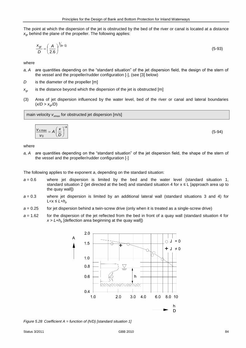
Principles for the Design of Bank and Bottom Protection for Inland Waterways
Status 3/2011 GBB 2010 84
The point at which the dispersion of the jet is obstructed by the bed of the river or canal is located at a distance xgr behind the plane of the propeller. The following applies:
)1(a1
gr
6.2
A
D
x (5-93)
where
a, A are quantities depending on the “standard situation” of the jet dispersion field, the design of the stern of the vessel and the propeller/rudder configuration [-], (see [3] below)
D is the diameter of the propeller [m]
xgr is the distance beyond which the dispersion of the jet is obstructed [m]
(3) Area of jet dispersion influenced by the water level, bed of the river or canal and lateral boundaries (x/D > xgr/D)
main velocity vxmax for obstructed jet dispersion [m/s]
D
xA
v
v x
a
0
max (5-94)
where
a, A are quantities depending on the “standard situation” of the jet dispersion field, the shape of the stern of the vessel and the propeller/rudder configuration [-]
The following applies to the exponent a, depending on the standard situation:
a = 0.6 where jet dispersion is limited by the bed and the water level (standard situation 1, standard situation 2 (jet directed at the bed) and standard situation 4 for x ≤ L [approach area up to the quay wall])
a = 0.3 where jet dispersion is limited by an additional lateral wall (standard situations 3 and 4) for L<x ≤ L+hp
a = 0.25 for jet dispersion behind a twin-screw drive (only when it is treated as a single-screw drive)
a = 1.62 for the dispersion of the jet reflected from the bed in front of a quay wall (standard situation 4 for x > L+hp [deflection area beginning at the quay wall])
Figure 5.28 Coefficient A = function of (h/D) [standard situation 1]

Principles for the Design of Bank and Bottom Protection for Inland Waterways
Status 3/2011 GBB 2010 85
The following applies to coefficient A:
(1) For jet dispersion limited only by the bed and water level behind a propeller without jet splitting, i.e. for propellers without a middle rudder behind them or for ducted propellers (in this case also followed by a middle rudder) for 1.0 ≤ h/D ≤ 9
(standard situation 1, see Figure 5.28):
/D)(h - A 092.0e88.1 (5-95)
where
h is the depth of water [m].
(2) In the case of jet splitting through a middle rudder behind the propeller (0.7 ≤ hp /D ≤ 5)
(standard situations 2 and 3, see Figure 5.29):
DhA p061,0
e88.1
(5-96)
where
hp is the height of the propeller axis above the bed [m]
Figure 5.29 Coefficient A = function of (hp /D) [standard situation 2]
(3) For twin-screw drives (approximation) A = 0.9 = constant when calculating as for a single screw drive (interaction of the jets outweighs the influence of the water depth)
(4) Where the dispersion field is limited by a deflecting wall located in the direction of propagation of the jet (for the jets reflected from the bed and wall, x ≥ L+hp)
(standard situation 4, see Figure 5.30):
62.1
p
0
max )(
D
hL
v
LvA
x (5-97)
where
hp is the height of the propeller axis above the bed (length of the jet deflected downwards at the wall, measured from wall to bed) [m]
L is the distance between the deflecting wall and the plane of the propeller [m]
D is the diameter of the propeller [m]
vxmax(L) is the main velocity at distance L behind the plane of the propeller [m/s]

Principles for the Design of Bank and Bottom Protection for Inland Waterways
Status 3/2011 GBB 2010 86
The jet velocity relevant to scour at the toe of the quay wall is taken as the velocity occurring at the point where x = L (see Figure 5.30).
Figure 5.30 Jet dispersion characteristics of the twin-screw drive of an ocean-going vessel where the jet is reflected from a deflecting wall at the deflection distances L / D = 3.0 and 5.0 (standard situation 4) /Römisch 1975/
5.6.3.3 Calculation of the distribution of the jet velocity orthogonal to the jet axis
The distribution of the jet velocity vxr orthogonal to the jet axis in the area of jet impact is governed by
- the position of the jet axis above or at the bed at a distance x from the propeller plane (see 5.6.3.1) and
- the main velocity vxmax
N.B.: vxmax is calculated in the eqs. (5-91), (5-92) and (5-94) with
v0 where vS = 0 and J = 0
v0J when vS 0 and J 0
taking into account the radial velocity distribution:
e
2x2.22
max
xr xr -
xv
v (5-98)
where
rx is the radial distance of the considered point, e.g. the bed, from the jet axis at a distance x from the plane of the propeller [m]
vxr is the jet velocity relative to the ship in the radius rx [m/s]
The jet velocity vxr1 at the bed or bank, taking into account the ship speed is obtained as an approximation as follows:
J0
Sxr1xr
v
v1vv (5-99)
where
vxr is the jet velocity relative to the ship in the radius rx [m/s]
vS is the ship speed through water [m/s]; when applicable use signed: vS is negative if the movement of the
ship and the propeller jet point in the same direction, e.g. when the vessel is stopping.
v0J is the induced initial velocity at J > 0 [m/s]

Principles for the Design of Bank and Bottom Protection for Inland Waterways
Status 3/2011 GBB 2010 87
The following correlation between rx, x and hp is obtained for loads on a plane river or canal bed (cf. Figure 5.31):
00px cos/sin xhr (5-100)
0x0S sincos rxx (5-101)
Figure 5.31 Geometrical definitions for the calculation of the distribution of near-bed flow velocities orthogonal to the jet axis
The near-bed flow velocity calculated using eqs. (5-98) to (5-101) initially increases in the x-direction, before decreasing again. The maximum near-bed flow velocity vxr is referred to as vBmax for the purpose of determining the size of the armour stones. The following equation can be used to calculate the position of this maximum for rough estimates:
B
p
maxS,tan
hx (5-102)
where
hp is the height of the propeller axis above the bed [m]
xS,max is the position of the maximum near-bed flow velocity behind the centre of rotation of the propeller plane [m]
B is the mean angle of diversion
B = 8.5° for standard situations 1 and 4 at xS,max < L
B = 13° for standard situations 2 and 3 (see 5.6.3.1)
Allowance for the influence of the propeller advance ratio on v0 and thus on vxmax and vBmax has already been made in eqs. (5-85) to (5-89). However, the velocity of the impact on the bed of the waterway is also affected by the propeller advance ratio and is calculated approximately by eq. (5-104).
The standard situations describing the jet dispersion characteristics in 5.6.3.1 can be used analogously to determine the loads on slopes rising in the same direction as the jet. The maximum flow velocity at the bed and slope must be determined by eq. (5-98) taking account of the geometrical boundary conditions shown in Figure 5.32 and Figure 6.1 and in accordance with eq. (6-4). A meaningful assumption of the largest angle between the ship’s axis and the bank line must be made. Large angles occur, for example, when ships navigate bends.
When a ship casts off, the jet strikes the slope because it is deflected at the rudder. The smallest angle relevant
to the design, St
, between a perpendicular to the slope line and the axis of the deflected jet may be 15°
(see Figure 6.1). The deflection of the jet reduces the jet velocity to around 85% of its initial value at the propeller.
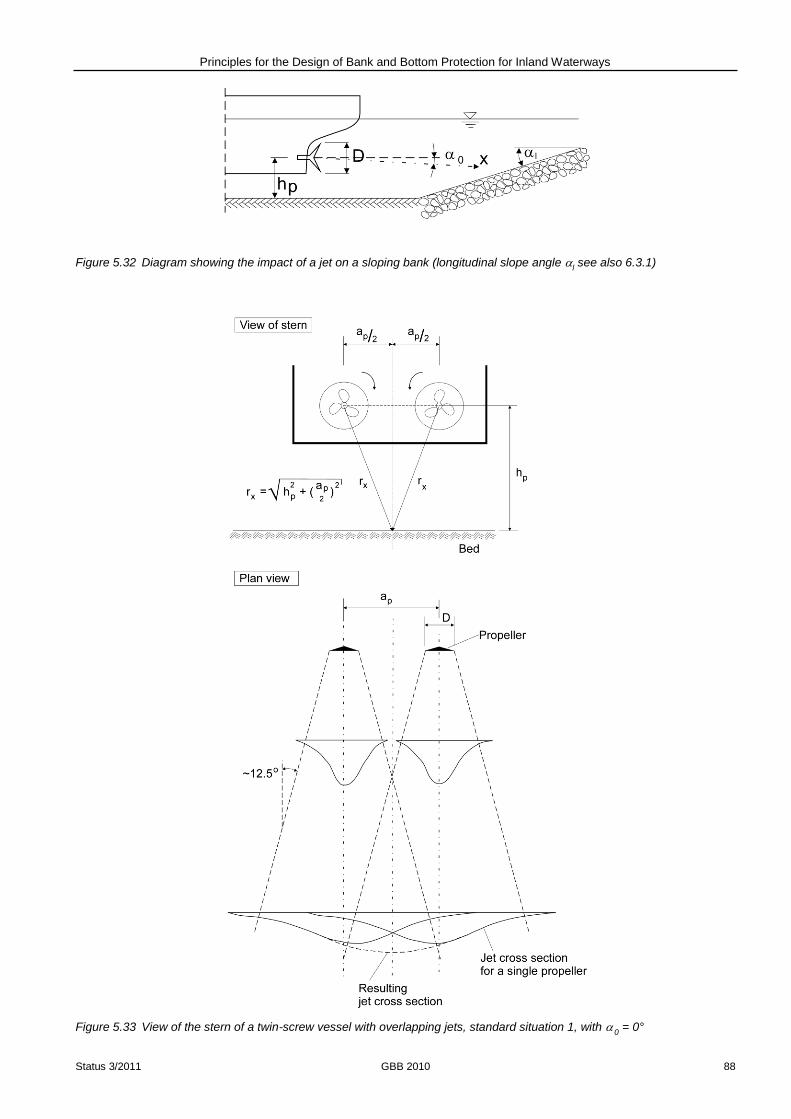
Principles for the Design of Bank and Bottom Protection for Inland Waterways
Status 3/2011 GBB 2010 88
Figure 5.32 Diagram showing the impact of a jet on a sloping bank (longitudinal slope angle l see also 6.3.1)
Figure 5.33 View of the stern of a twin-screw vessel with overlapping jets, standard situation 1, with 0 = 0°

Principles for the Design of Bank and Bottom Protection for Inland Waterways
Status 3/2011 GBB 2010 89
5.6.3.4 Multi screw drives
In the case of multi-screw drives, the jet dispersion for each propeller must first be considered separately by means of the algorithms given in Chapters 5.6.1 to 5.6.3.3 in accordance with /Römisch 1994/. The parameter a
must be chosen as if there were two single-screw drives (a ≠ 0.25). The vxr values can be added by way of
approximation in order to determine how the drives act in combination. With 0 = 0° in standard situation 1 the
geometrical boundary conditions shown in Figure 5.33 are obtained.
For 0 0°, if jets are dispersed laterally or strike the bank at an angle, a sketch with all the relevant
geometrical dimensions is recommended in order to obtain a meaningful superposition of the two partial jets.
The values of the jet velocity at the bed obtained for twin-screw vessels when the propellers counter-rotate towards each other may be higher than those obtained by addition, as indicated in Figure 5.33.
Note: A generalised calculation method for jet superposition is shown in Annex E. As an approximation, multi-screw drives with parameters (a = 0.25 and A = 0.9) as stated in eq. (5-94) may also be treated as single-screw drives.
5.6.4 Simplified calculation of the maximum near bed velocity
A simplified method of calculating the maximum near-bed velocity for propeller advance ratios J = 0 and J ≠ 0 in some cases is described below for single and multi-screw vessels. The method can be used only if the jets are not superposed.
Ship speed through water vS = 0
The maximum near-bed velocity at the point of impact of the propeller jet vBmax can be estimated as follows for
the standard jet dispersion situations 1, 2 and 3 for J = 0 as an approximation (see 5.6.3.1):
maximum near-bed velocity at the point of impact vBmax for J = 0 (simplified calculation) [m/s]
0p
Bmax vh
DEv
(5-103)
where
D is the diameter of the propeller [m]
hp is the height of the propeller axis above the bed [m]
E is the coefficient for characterisation of stern shape and rudder configuration [-] (see Figure 5.34)
E = 0.71 for slender sterns with a middle rudder
E = 0.42 for slender sterns without a middle rudder
E = 0.25 for modern inland navigation craft with a tunnel stern and twin rudders
v0 is the induced initial velocity at J = 0 [m/s], see 5.6.1

Principles for the Design of Bank and Bottom Protection for Inland Waterways
Status 3/2011 GBB 2010 90
Figure 5.34 Change in relative maximum near-bed velocity of the propeller jet vBmax / v0 = as a function of (hp /D, E)
Ship speed through water vS ≠ 0
When a ship casts off, i.e. when the propeller advance ratio is increasing, there is a decrease in the induced initial velocity relative to the bed and bank and, thus of the associated velocity at which the propeller jet strikes the boundaries of the fairway.
The maximum near-bed velocity vBmax1 at the propeller advance ratio J ≠ 0 can be calculated approximately in
this case as follows:
maximum near-bed velocity at the point of impact vBmax1 for J ≠ 0 (simplified calculation) [m/s]
J
SBB
v
vvv
0
max1max 1 (5-104)
where
vBmax is the maximum near-bed velocity at the point of impact [m/s] for vS = 0 or J = 0 (simplified calculation)
vBmax1 is the maximum near-bed velocity at the point of impact [m/s] for vS ≠ 0 or J = 0
vS is the ship speed through water [m/s];
when applicable use signed: vS is negative if the movement of the ship and the propeller jet point in the
same direction, e.g. when the vessel is stopping.
v0J is the induced initial velocity [m/s] at J > 0, according to 5.6.2
For narrow fairway conditions (e.g. lock exits), the reductions in the near-bed velocities referred to above are negligible due to the very low ship speeds that are possible owing to the extreme limitation of the fairway. In this case, the load conditions can be assumed as for J = 0.
5.6.5 Flow velocity at the bed allowing for the surrounding flow field
In the case of a moving ship, the flow velocity close to the bed that is critical for the sizing of the armour layer material for bed protection consists, in addition to the propulsion jet velocity, of the return flow, the wake and the current in the canal or river. It should be remembered that
- the flow velocity near the bed is lower
- the return flow underneath the ship may be hindered by the hull of the ship
- even the wake (water carried along by the ship in the direction of motion) can act against the flow due to propulsion

Principles for the Design of Bank and Bottom Protection for Inland Waterways
Status 3/2011 GBB 2010 91
Thus the flow velocity vmax,S at the bed that is critical to the design is calculated for the special case of flow
parallel to the ship’s path for upstream and downstream motion as follows:
upstream: vmax,S,Berg
= vmax,S + v
fl,bem + v
Nach,bem (5-105)
downstream: vmax,S,Tal = v
max,S – vfl,bem
+ vNach,bem
(5-106)
where
vmax,S,Berg is the flow velocity [m/s] critical to the design at the bed allowing for the surrounding flow field during upstream motion
vmax,S,Tal is the flow velocity [m/s] critical to the design at the bed allowing for the surrounding flow field during downstream motion
vmax,S is the maximum flow velocity [m/s] at the bed without allowing for the surrounding flow field
vmax,S = vxr or vxr1 calculated precisely according to 5.6.3.3
vmax,S = vBmax or vBmax1 simplified calculation according to 5.6.4
vfl,bem is the flow velocity [m/s] within the propeller jet close to bed or revetment at a distance equal to the
boundary layer from the revetment according to eq. (5-107)
vNach,bem is the wake [m/s] close to the bed according to eq. (5-108)
The flow velocity close to the bed or revetment vfl,bem should be determined within the propeller jet at the
boundary layer distance of G from the revetment. As an approximation, G = 1 m can be assumed. By
assuming a 1/7 power law for the vertical flow velocity distribution, the following can be applied for the flow
velocity at the bed, that is, at the boundary layer distance G:
m
71
Gmbemfl,
7
8v
hvv
(5-107)
where
vfl,bem is the flow velocity [m/s] close to the bed or revetment
vm is the mean flow velocity [m/s] as the depth mean in the path of the ship
G is the boundary layer distance [m]
h is the mean water depth [m] of the body of water
Note: The 1/7 power law can be applied for beds or banks consisting of material ranging from gravel to armour stones.
The wake vNach,Bem close to the bed can be estimated as follows according to /Maynord 2004/:
S
81,1
BemNach, 78.0 vT
hv
(5-108)
where
vNach,Bem is the velocity of the wake [m/s] close to the bed
T is the draught [m]
vS is the ship speed through water [m/s]
It should be remembered that this equation states the maximum value behind the ship. However, this does not necessarily occur at the same point as the maximum propeller jet velocity. Strictly speaking, the distribution of the wake velocity behind the ship should be considered. However, the above equation is considered to be adequate for an estimation of the flow velocity vmax,S at the bed.

Principles for the Design of Bank and Bottom Protection for Inland Waterways
Status 3/2011 GBB 2010 92
5.6.6 Load due to bow thrusters
According to /Schokking 2002/ revetments can be damaged by bow thrusters operated in the vicinity of mooring places and such damage needs to be taken into account in the design. The ship speed is negligible in this case and vS = 0 will be assumed below. According to trials with models the equations stated below can also be taken
as approximations for ship speeds of up to around 5 km/h. A distinction is made between temporary load during a mooring manoeuvre and persistent load, and between load on a sloping bank (slope inclination < 45°) and on the bed in front of a vertical bank (quay wall), see Figure 5.35. This load is not generally relevant to the design if the vessel is moving (vS ≠ 0) as, in that case, the jet is deflected.
Figure 5.35 Jet dispersion for load from bow thrusters; a) sloping bank, b) quay wall, where the jet is deflected towards the bed of the river or canal
= slope angle αl = longitudunal slope angle, see Figure 6.1 and eq. (6-4)
The induced initial velocity v0 corresponds approximately to that of a ducted propeller with an advance ratio of J = 0. Depending on the engine power, the following equation applies in accordance with /EAU 2004/; /Blaauw, Kaa 1978/
31
2W
Bug0 )(1.1
D
Pv
(5-109)
where
PBug is the installed power of the bow thruster [W] see Table 5.1
N.B.: The value is stated in [kW] in Table 5.1
D is the duct diameter diameter of the propeller of the bow thruster [m]
ρW is the density of the water [kg/m3]
or eq. (5-80) applies, depending on the thrust coefficient
DPT,NennN0 13.1 KDnfv (5-110)

Principles for the Design of Bank and Bottom Protection for Inland Waterways
Status 3/2011 GBB 2010 93
where
fN is the factor for the applicable propeller rotation rate [-]
recommended according to /EAU 2004/:
fN ≈ 0.75 for a starting manoeuvre from a stationary position
KT,DP is the thrust coefficient of a ducted propeller [-] for J = 0 as in eq. (5-80)
nNenn is the design propeller rotation rate [1/s], see Table 5.1
N.B.: in Table 5.1 values are given as [1/min]
v0 is the induced initial velocity at J = 0 [m/s]
The decrease in the induced initial velocity is lower for bow thrusters than for free propellers. The following applies to the maximum axial flow velocity (main velocity) vxmax at a sloping bank and as derived from
measurements by /Schokking 2002/:
maximum axial flow velocity of a bow thruster at a sloping bank vxmax [m/s]
0max vv x for 0.1D
x
(5-111)
31
0max
D
xvv x for 0.1
D
x
where
D is the duct diameter diameter of the propeller [m]
vxmax is the maximum axial flow velocity, main velocity [m/s]
v0 is the induced initial velocity [m/s]
x is the distance from the outlet side of the bow thruster [m]
The design value at the slope occurs where x = L.
At the toe of a quay wall, the maximum jet velocity at the bed vmax,S,K is (according to /Blokland 1994/):
P
0S,Kmax, 0.1
h
Dvv for 8.1
P
h
L
(5-112)
P
0S,Kmax, 8.2
hL
Dvv
for 8.1
P
h
L
where
hP is the height of the bow thruster axis above the bed [m]
L is the distance between the plane of the bow thruster outlet and the quay wall [m]
Vmax,S,K is the maximum flow velocity at the bed at the toe of the quay wall [m/s]
The further decrease in the jet at the bed vmax,S,xK after deflection can be calculated as follows in the same way
as for the propeller jet of the main drive as a function of the distance xK from the quay wall:
62.1
PS,Kmax,xKS,max,
x
hLvv (5-113)

Principles for the Design of Bank and Bottom Protection for Inland Waterways
Status 3/2011 GBB 2010 94
where
x is the distance along the jet axis measured from the jet outlet to the quay wall and then to the bed of the river or canal [m] x = L + hP + xK
xK is the distance of the deflected jet from the quay wall measured along the bed of the river or canal [m]
Vmax,S,xK is the changed maximum flow velocity at the bed after deflection at a distance of xK from the quay
wall [m/s]
The size of stones required for ungrouted revetments is determined as in Chapter 6.3. Chapter 8 deals with how to allow for partial grouting.
5.7 Waves in general, wave deformation and water levels
Wind waves and wind set-up
In addition to the ship-induced waves, other waves may occur in bodies of water as a result of the action of wind. Their height and length depends on the direction of the wind, its speed and the duration of the wind action. In individual cases, it may be necessary to consider their combined impact with other waves. This should be examined, for example, in the case of waterways on large plains (Rhine Lowlands, North German Plain) and for long, wide reaches of waterways (impoundments). Wind waves can usually be disregarded in the case of canals, although wind set-up may be of relevance, especially in long impoundments. Further information on wind data, fetch and minimum impact duration, wind set-up and the height and periodicity of wind waves can be found in GBB 2004 /BAW 2005/.
Wave deformation
All wave heights determined in 5.4 to 5.6 depend on waves being able to propagate unhindered. This applies in most design cases. However, in certain situations, the wave front is subject to numerous disturbances and influences (structures, variations in the depth of the water, angles of approach) that change the height of the wave. The environment around the planned revetment must therefore be examined to determine how it is likely to affect the wave height at the design point. Wave shoaling and breaking of waves, diffraction, refraction and/or reflection may occur. Further infomation can be found in GBB 2004 /BAW 2005/.
Other waves
Other causes of variations in the water level besides the short-periodic ship- and wind-induced waves may be long-periodic waves. These include positive surge waves and drawdown waves, tidal waves and flood waves. Depending on the design situation and problem, these types of wave must be added cumulatively to the waves originating in other ways (wind, ship).

Principles for the Design of Bank and Bottom Protection for Inland Waterways
Status 3/2011 GBB 2010 95
6 Hydraulic design of unbound armour stone cover layers
6.1 General remarks
The hydraulic design of unbound armour stone cover layers must be based on the action of waves and/or currents as described in Chapter 4.
Experience and tests conducted with models have shown that the resistance of an unbound armour stone cover layer to erosion due to the actions of waves or currents is affected by the following parameters:
size or weight of individual armour stones (stone size) and bulk density
installation thickness of the riprap
The design rules for varying hydraulic loads developed on the basis of experience and in model tests will be explained below. The design parameter is the armour stone size D50 (size of armour stones in the cover layer defined by sieve at 50% sieve throughput), or Dn50 (nominal stone size at 50% sieve throughput). More detailed explanations of the armour stone sizes and their implementation in standardised stone size classes are shown in 6.8.
6.2 Armour stone size required to resist load caused by transversal stern waves
The minimum mean stone size D50 of the armour layer material of bank revetments that is required to resist displacement under normal sailing conditions can be calculated for the maximum height of any transversal stern wave by means of the following equation:
armour stone size D50 required to resist transversal stern waves [m]
mB
HD
1/3
W
WSB
Bem50
(6-1)
where
B'B is the stability coefficient [-], derived from field tests /BAW 2009/
B'B= 1.5 (lower limit of measured values) – 2.3 (mean measured value)
The following is recommended for the design:
B'B=1.5 if the design case occurs frequently or if damage to the revetment should be completely avoided
B'B=2.3 if the design case occurs infrequently or when a limited amount of maintenance is acceptable
D50 is the required stone size (stone size defined by sieve) at 50% mass throughput of the cumulative line [m]
HBem is the design wave height [m],
HBem = MAX {Hu,Heck; Hu,Heck,StBem ; HSek,q}
Hu,Heck stern wave height of the primary wave system according to 5.5.4.4 ,eq. (5-32) and Figure 5.12
Hu,Heck,StBem design value according to eq. (5-53) in 5.5.5.1 for distance case B
HSek,q height of pure transversal stern waves of the secondary wave system according to 5.5.5.2, eq.
(5-61), limited by eq. (5-65)
m is the slope inclination m = cot β [-], 2 m 5
N.B.: mK,äqui should not be used here, but the actual slope inclination mrts or mlks
is the slope angle [°]
ρW is the density of the water [kg/m3]
ρS bulk density of the armour stones [kg/m³]
N.B.: /TLW 2003/

Principles for the Design of Bank and Bottom Protection for Inland Waterways
Status 3/2011 GBB 2010 96
The design equation is based on Hudson’s equation for determining the stone size required to withstand wave run-up. In the latter the slope inclination influences both the type of breaker and the run-off velocity of the wave which causes the greatest loads. For these waves, which usually run parallel to the bank, the influence m
- 1/3 on
D50 is overestimated, particularly for small, gentle slope inclinations. Eq. (6-1) should therefore only be used for engineered slopes with inclinations m of approximately 2-5.
The following can be assumed to allow for the influence of the repose angle of the armourr layer material 'D,hydr
and of the slope angle in a first approximation in analogy to the design for slope supply flow:
W
WS*B
Böu,Heck50
B
CHD (6-2)
where
B*B is the coefficient for frequency of occurrence [-]
B*B ≈ 2.0 if the design case occurs frequently or if damage to the revetment should be completely avoided
B*B ≈ 3.0 if the design case occurs infrequently or when a limited amount of maintenance is acceptable
CBö is the factor for consideration of the influence of the slope [-]; for definition see eq. (6-8) in 6.6.1
Hu,Heck is the stern wave height [m] according to 5.5.4.4, eq. (5-32) and Figure 5.12 or the secondary transversal wave height according to 5.5.5.2, eq. (5-61), limited by eq. (5-65) or the design value Hu,Heck,StBem according to eq. (5-53) in 5.5.5.1 for distance case B
6.3 Stone size required to resist flow due to propulsion
6.3.1 Stone size required to resist attack from propeller jet
In order to ensure the stability of the bed in manoeuvring areas without significant degree of scouring, the mean armour stone size D50 of the armour layer material of the bed protection that is required for the maximum velocity vxr (see 5.6.3.3) or vBmax (see 5.6.4) can be determined as follows:
stone size D50 required to resist propeller jet [m]
W
WS
Smax,
S50
1
g
vBD
2
(6-3)
where
BS is the coefficient for attack from propeller jet on a plane bed
BS ≈ 1.23 for ships without a middle rudder and inland navigation vessels with a tunnel stern, standard situations 1 and 4, (see 5.6.3.1) and bow thrusters (see 5.6.6)
BS ≈ 0.64 for ships with a middle rudder; standard situations 2 and 3 (see 5.6.3.1)
vmax,S is the maximum flow velocity at the bed [m/s]
vmax,S = vxr, or according to exact calculation, vxr1, ; see 5.6.3.3
vmax,S = vBmax or vBmax1 (simplified calculation) see 5.6.4
vmax,S = vmax,S,Berg or vmax,S,Tal in the special case of flow parallel to the ship’s path, see 5.6.5

Principles for the Design of Bank and Bottom Protection for Inland Waterways
Status 3/2011 GBB 2010 97
If the jet from the main drive or bow thrusters strikes a bank, the value of BS stated above must be replaced with BS,Bö as in eq. (6-4), depending on the longitudinal slope angle and the cross slope angle in the direction of the jet (see Figure 6.1).
Figure 6.1 Diagram showing propeller jet attack on a bank during (a) a turning manoeuvre or (b) deflection of the jet during a casting-off manoeuvre
Stq
Stl
2
hydrD,
2
q
hydrD,
hydrD,l
l
ql
SBöS,
sintantan
costantan
'tan
tan1cos
'sin
)'sin(
/
K
K
KKK
KBB
(6-4)
where
K is the inclination coefficient [-]
K l is the longitudinal slope coefficient [-]
Kq is the cross slope coefficient [-]
l is the longitudinal slope angle [°]
q is the cross slope angle [°]
is the slope angle [°], = arctan (1/m)
St is the angle between jet axis and a perpendicular to the slope line (angle of impact) [°]
'D,hydr is the angle of repose of the armour layer material [°], normally 45°
Note: For the hydraulic design a lower limit of the angle of repose will be assumed.

Principles for the Design of Bank and Bottom Protection for Inland Waterways
Status 3/2011 GBB 2010 98
6.3.2 Stone size required to limit the depth of scour due to propeller jet
The equations stated by /Römisch 1975/ and /Ducker, Miller 1996/ can be used for estimating the depth of scour caused by propeller jet or the stone size required for a given tolerated scour depth:
13
*85
*
m85
Kolk 1.0
B
BC
D
hfor 4.11
*85
*
B
B
25.2
*85
*
m85
Kolk 6.4
B
BC
D
hfor 4.1
*85
*
B
B
(6-5)
85
Smax,*
' Dg
vB
KBB *0,85
*85
where
*B is the load coefficient [-]
*85B is the stability coefficient for slopes [-]
*0,85B is the stability coefficient, in general [-]
25.1*0,85 B standard situations 1 and 4 (see 5.6.3.1) and bow thrusters (see 5.6.6)
73.1*0,85 B standard situations 2 and 3 (see 5.6.3.1)
Cm is the coefficient for the duration of the load [-]
Cm = 1.0 for persistent load
Cm = 0.3 for temporary load during manoeuvring of ship and for scouring in revetments comprising common types of armour stones (does not apply to sand or gravel)
g' is the relative density [m/s2], g' = g ((S -W)/W)
hKolk is the depth of scour below the bed of the river or canal [m]
K is the inclination coefficient [-], see eq. (6-4)
vmax,S is the maximum flow velocity at the bed [m/s]
- for main drive vBmax or vBmax1 according to 5.6.4
- for bow thruster vxmax or vmax,S,K according to 5.6.6
W is the density of the water [kg/m3]
S is the density of the riprap material [kg/m3]
In the case of small stone sizes and large scour depths, the development of scour over time must be observed more precisely than with the coefficient Cm /Gaudio, Marion 2003/.
Solving of the eq. (6-5) for D85 with a given tolerated scour depth leads to ambiguities. For this reason, when
using the equations, hKolk should be plotted as a function of D85 and a plausible value for erf D85 read from this.
In addition, the following condition should be complied with:

Principles for the Design of Bank and Bottom Protection for Inland Waterways
Status 3/2011 GBB 2010 99
50
50
8585 Derf
Dvorh
DvorhDerf (6-6)
where
erf D50 is the required stone size at 50% sieve throughput [cm]
erf D85 is the required stone size at 85% sieve throughput [cm]
vorh D50 is the existing stone size at 50% sieve throughput [cm] of the mean grading curve
vorh D85 is the existing stone size at 85% sieve throughput [cm] of the mean grading curve
6.4 Armour stone size required to resist load due to secondary diverging waves
The wave crests of the diverging waves propagating from the bow and stern of a ship strike the bank at an
angle W of approximately 55° when the ship is underway parallel to the bank and when 8.0mS hgv
(see Figure 5.20). According to /Verhey, Bogaerts 1989/, the ship-induced secondary waves can be treated as
incoming waves if the wave height is reduced as follows by the factor cos W:
nominal armour stone size Dn50 required to resist secondary diverging waves [m]
21
Sek
S
W
WS
21
21
WSek50n
tan
sincos25.2
cos
H
HD
(6-7)
where
HSek is the height of the secondary waves [m] in accordance with 5.5.5, possibly with superposed wind waves as described in 5.7
S is the wave length of the secondary diverging wave [m] in accordance with eq. (5-59)
is the slope angle [°]
W is the angle between the wave crest of the secondary diverging wave and the bank line [°], normally
W = 55° see Figure 5.20
is the surf similarity parameter [-]
The equations (6-1) and (6-2) may be used as approximations for transversal stern waves that run parallel to the bank. HSek,q according to eq. (5-61), is thus to be substituted for Hu,Heck limited by eq. (5-65).
6.5 Stone size required to resist wind waves or the combined load from ship
induced waves and wind waves
If the armour layer is affected only by load from wind waves – which may be the case for large water surfaces in inland regions – the required mean nominal stone size Dn50 can be determined according to 6.5 in the GBB
2004 /BAW 2005/.
In rare cases, the secondary diverging waves and wind waves may be unfavourably superposed, usually behind the ship. More details on this may be found in 6.6 in the GBB 2004 /BAW 2005/.
6.6 Stone size required to resist attack by currents
In addition to load caused by ship-induced waves and possibly from wind waves, the planned armour layer must also withstand attack by currents flowing parallel to the bank and bottom of the river or canal. This results from the natural current, the return flow and in some cases from the superposition of these two above mentioned parameters or from the slope supply flow of the breaking stern wave.

Principles for the Design of Bank and Bottom Protection for Inland Waterways
Status 3/2011 GBB 2010 100
6.6.1 Stone size required to resist attack by currents flowing largely parallel to the slope
The following equation may be used to obtain a rough estimate of the stone size /PIANC 1987a/:
stone size D50 required to resist currents [m]
g
vCCD
W
WS
2max
BöIsb50
1
(6-8)
where
CBö is a factor for considering the influence of the slope [-], CBö=1/k
CIsb is a factor according to Isbash [-], CIsb ≈ 0.7
D50 is the required stone size (stone size defined by sieve) at 50% mass throughput of the cumulative line [m]
g is the acceleration due to gravity [m/s²]
k is the factor [-]
k = cosβ [1 - (tan²β/tan² 'D,hydr)]0.5
(6-9)
vmax is the maximum flow velocity [m/s] made up of return flow and flow velocity vStr,Ufer in the vicinity of the bank (at a distance equal to the thickness of the boundary layer of the return flow field) according to eqs. (5-39) and (5-40) in 5.5.4.6
β is the slope angle [°]
'D,hydr is the repose angle of the armour layer material [°], usually 'D,hydr = 45°
ρW is the density of the water [kg/m3]
ρS is the density of the riprap [kg/m3]
Eq. (6-8) is based on a limit definition by Isbash /DVWK 1997/ that ensures stability against pure attack only by currents for horizontal and gently sloping river and canal beds. Compared to other methods, eq. (6-8) yields higher values /DVWK 1997/; /Söhngen, Koll 1997/.
Extending the basic equation by the factor CBö describes the increase in the required nominal stone size Dn50
due to the slope angle β and the angle of repose 'D,hydr of the armour layer material of the riprap. The
dependency CBö = function of (β, 'D,hydr) can be seen in Figure 6.2.
The point at which the natural bed material (adjacent to the toe of the revetment) begins to move can be estimated by means of the methods described by Hjulström (empirical method; correlation between the mean flow velocity and mean stone size), Shields (semi-empirical method; correlation between the velocity of the shear stress at the bed and the roughness of the bed; iterative solution) or Bonnefille (like Shields; direct solution), which are explained in detail in /Dittrich 1998/. All of these methods apply to uniform bed material (U = D60/D10 < 3) with stone sizes D < 100 mm.

Principles for the Design of Bank and Bottom Protection for Inland Waterways
Status 3/2011 GBB 2010 101
Figure 6.2 Dependence of the factor CBö on the slope angle or the slope inclination m and the angle of shearing
resistance 'D,hydr
6.6.2 Stone size required to resist load on the slope due to slope supply flow
The coefficient CIsb in eq. (6-8) must be reduced for loads due to the highly turbulent temporary currents, partly
mixed with air and parallel to the slope, that occur when a transversal stern wave breaks (surf similarity parameter, see Figure 5.15 in 5.5.4.5) and the resulting depression is filled from astern. According to this, with the maximum value of the flow velocity umax and allowing for the natural current, the following stone size D50 is
obtained:
armour stone size D50 required to resist slope supply flow [m]
W
WS
2Bmax,
Bö50
15.0
g
uCD (6-10)
where
umax,B is the design velocity resulting from the slope supply flow [m/s] in consideration of the natural current
close to the bank according to eq. (5-41) and (5-42) in 5.5.4.6
Allowance must be made for boundary effects as the depth of water in the slope supply flow is small, which corresponds more or less to the wave height. The load acting on a slope is therefore greater for rough slopes than for slopes stabilised with small stone sizes. This effect can be taken into account as an approximation as follows by introducing the height of the stern waves in accordance with /BAW 2009/.
armour stone size D50 [m] allowing for the stern wave height
23
31
Hecku,W
WS
Bö2
Bmax,50
4.1
Hg
CuD
(6-11)

Principles for the Design of Bank and Bottom Protection for Inland Waterways
Status 3/2011 GBB 2010 102
where
Hu,Heck is the maximum height of the stern wave [m] including the secondary wave component near the slope in accordance with 5.5.4.4, eq. (5-32)
The above equation can only provide an initial estimate of the armour stone size required for a revetment owing to the uncertainties in the determination of umax,B. However, they show that the ship speed and the height of the
breaking stern wave, on which umax,B largely depends, are crucial to determining the stone size.
6.7 Stone size required for all types of load
Sailing at normal speed
As the banks are subject to all types of load simultaneously when a vessel is underway at normal speed, the determining of an acceptable individual stone size must also take account of all design formulae according to the proportion of their impact. This leads to a weighting concept that allows for the physical relationships of the various load variables and takes these equally into consideration in the calculation of the size of the armour stones.
- Transversal stern wave and slope supply flow are part of the primary wave field of the flow around the ship, which by means of the eqs. (6-1), (6-2), (6-10) and (6-11) result in stone sizes, each of which accounts for 25%.
- The return flow is a separate process, meaning that eq. (6-8) applies 100%.
- In the secondary wave field an armour stone size for diverging waves is obtained using only eq. (6-7) and, for the transversal waves, from eqs. (6-1) and (6-2) in equal parts; for diverging and transversal waves the maximum value should be selected.
All three groups yield a result for the individual armour stone size, of which in each case the maximum size is to be taken as relevant for design. The method is shown in a diagram in Figure 6.3.
Figure 6.3 Diagram of weighting concept to consider all types of load when determining the required size of individual armour stones
Manoeuvring
For manoeuvring situations the eqs. (6-3), (6-4) and (6-5) are to be used to determine the size of individual stones.
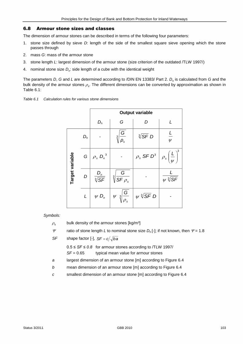
Principles for the Design of Bank and Bottom Protection for Inland Waterways
Status 3/2011 GBB 2010 103
6.8 Armour stone sizes and classes
The dimension of armour stones can be described in terms of the following four parameters:
1. stone size defined by sieve D: length of the side of the smallest square sieve opening which the stone passes through
2. mass G: mass of the armour stone
3. stone length L: largest dimension of the armour stone (size criterion of the outdated /TLW 1997/)
4. nominal stone size Dn: side length of a cube with the identical weight
The parameters D, G and L are determined according to /DIN EN 13383/ Part 2. Dn is calculated from G and the
bulk density of the armour stones s. The different dimensions can be converted by approximation as shown in
Table 6.1:
Table 6.1 Calculation rules for various stone dimensions
Output variable
Dn G D L
Targ
et
vari
ab
le
Dn - 3
sρ
G DSF3
L
G 3
ns D - 3DSFs
3
Ls
D 3 SF
Dn 3
sSF
G
-
3 SF
L
L nD 3
s
G
DSF3 -
Symbols:
s bulk density of the armour stones [kg/m³]
ratio of stone length L to nominal stone size Dn [-]; if not known, then = 1.8
SF shape factor [-], abcSF
0.5 ≤ SF ≤ 0.8 for armour stones according to /TLW 1997/
SF = 0.65 typical mean value for armour stones
a largest dimension of an armour stone [m] according to Figure 6.4
b mean dimension of an armour stone [m] according to Figure 6.4
c smallest dimension of an armour stone [m] according to Figure 6.4

Principles for the Design of Bank and Bottom Protection for Inland Waterways
Status 3/2011 GBB 2010 104
Figure 6.4 Definition of the dimensions a, b and c of an armour stone
A riprap revetment always consists of stones of varying sizes within certain limits. The size and the percentage of stones in the riprap can be seen in the cumulative line (particle size distribution) as shown in Figure 6.5 for stone size defined by sieve D.
Figure 6.5 Cumulative line defining stone size Dx
Explanatory remark: Gi corresponds to the proportion by mass of a screening sample which passes through a sieve with opening size Dio, but is retained on a sieve with opening size Diu.
The variable Dx can be derived from the cumulative line. Dx is the stone size, which is not exceeded by X mass percent of a stone fraction. The design value for loose armour stones is for the most part D50 (cf. 6.2 to 6.6).
The size Dx, which belongs to a percent by weight X, which lies between Xiu and Xio, can be calculated by log-linear interpolation (for description, see Figure 6.5)
iuio
iu
XX
XX
D
DDD
iu
ioiux (6-12)
The standardised stone classes with limits for permitted stone size distributions are shown in Part 1, “Specification”, of /DIN EN 13383/. The important parameters here are the lower and upper class limit. The size and permitted proportion of stones which lie below the lower class limit (undersized stones) or above the upper limit (oversized stones) are also stated.

Principles for the Design of Bank and Bottom Protection for Inland Waterways
Status 3/2011 GBB 2010 105
In the standard /DIN EN 13383/ small armour stones are defined by the sieve diameter D (side length of the square-meshed sieve) and known as CPx/y class (coarse particle, with x being the lower class limit [mm] and y the upper class limit). The larger stones are defined by their weight G as light weight class LMx/y (light mass, where x is the lower class limit [kg], and y the upper class limit [kg]) or heavy class HMx/y (heavy mass). The classes that are normally used for armour layers for inland waterways are CP90/250, LMB5/40 and LMB10/60 /Kayser 2006/. The standard /DIN EN 13383/ does not stipulate a 50% value (D50 or G50), as obtained from the hydraulic design. For an evenly spread cumulative line within the lower class limit Du and the upper class limit Do, D50 is calculated according to eq. (6-12) to:
5.0
u
ou50
D
DDD (6-13)
or G50 accordingly
5.0
u
ou50
G
GGG (6-14)
6.9 Minimum thickness of the armour layer
6.9.1 Minimum thickness as the basis for armour stone dimensioning
The applications of the design formulae mentioned in 6.2 to 6.6 for the required armour stone size presuppose that the individual armour stones together form a stable stone structure. An armour layer of loose armour stones must therefore have a minimum thickness of dD of the armour stones. This is obtained from the boundary conditions of various model tests, which are the basis of the design approaches /Dietz 1973/; /Hudson 1959/; Fuehrer, Römisch 1985/ and from the many years of experience in the operation of waterways /Kayser 2006/.
minimum required thickness of armour layer dD [m]
n50D 0.25.1min Dd (6-15)
where
min dD is the minimum required installation thickness of an armour layer [m]
Dn50 is the required mean nominal stone size [m]
If the uniformity coefficient U of the riprap is taken into consideration, the following thickness can be recommended as the minimum installation thickness for erosion-resistant riprap /Abromeit 1997/.
minimum required thickness of an armour layer min dD [m] allowing for unconformity
UDd n50D 1.5min (6-16)
where
Dn50 is the required mean nominal stone size [m]
D10 stone size at 10% sieve throughput [m]
D60 stone size at 60% sieve throughput [m]
min dD is the minimum required installation thickness of an armour layer [m]
U uniformity coefficient of the riprap [-]
U = D60/D10 (6-17)
The following criteria have been derived from experience in operating waterways /Kayser 2006/:

Principles for the Design of Bank and Bottom Protection for Inland Waterways
Status 3/2011 GBB 2010 106
minimum required thickness of an armour layer min dD [m] allowing for the upper limit of stone size distribution
ÜkD
oKlGrD
1.0min
1.33min
Ld
Ld
(6-18)
where
L length = largest dimension of an armour stone [m] according to /DIN EN 13383/
LoKlGr length L of an armour stone [m], which corresponds to the upper limit of a stone class
LÜk length L of an armour stone [m], which corresponds to the maximum permissible oversized stone of a stone class
The values LoKlGr and LÜk must normally be calculated on the basis of data available on a stone fraction. A stone fraction can be defined using the class limits (lower and upper class limit for length, mass or sieve diameter) or by means of a cumulative line (for length, mass or sieve diameter). The equation for the calculation of LoKlGr and LÜk are shown in Table 6.2, depending on this definition.
Table 6.2 Calculation of LoKlGr and LÜk (cf. Table 6.1)
Definition by
class limits cumulative line
LoK
lGr
weight
class 3
oKlGr
s
G
3
70
s
G
size class oKlGr3 DSF
903 DSF
length
class LoKlGr L90
LÜ
k
weight
class 3
Ük
s
G
3
100
s
G
size
class*
1.0
KlGr u
KlGr ooKlGr
3
D
DDSF
1003 DSF
length
class 1.33 LoKlGr L100
* For the size classes defined by class limits, a realistic estimate is formulated using the oversized stones of the 100-% value of the log-linear straight lines of the above graph.
Symbols:
ratio of stone length L to nominal stone size Dn [-]; if not known, then = 1.8
SF shape factor [-] see Table 6.1
s bulk density of the armour stones [kg/m³]
G stone mass [kg]
D stone size (stone size defined by sieve) [m]
L stone length [m]
Indices:
uKrGr lower limit of a stone class
oKrGr upper limit of a stone class
Ük maximum permitted oversize stone of a stone class

Principles for the Design of Bank and Bottom Protection for Inland Waterways
Status 3/2011 GBB 2010 107
6.9.2 Minimum thickness of an armour layer for protection purposes
The minimum thicknesses specified below must be complied with additionally in order to ensure the various protective functions of the armour layer /Abromeit 1997/.
The minimum thickness of an armour layer (on the bed) required to provide adequate safety against anchor cast regardless of the stone class used is:
filter geotextile on 6.0min
filter granular on 50.min
D
D
xmd
xmd (6-19)
where
min dD Minimum thickness of the armour layer
x is the additional thickness for different kinds of stone material [m]
x = 0 m when armour stones are used
x = 0.2 m for small-grained or ungraded material
The minimum thickness (at the slope) required to provide adequate safety against impacts by ships regardless of the stone class used is:
filter geotextile on 5.0min
filter granular on 30.min
D
D
xmd
xmd (6-20)
When using granular filters, the following minimum thickness of the armour layer should generally be adhered to, depending on the stone class used:
min dD ≥ 1.5 L50 + 0.10 m (6-21)
where
L50 is the armour stone length [m] at 50% mass throughput of the cumulative line
When using geotextile filters, the following minimum thickness of the armour layer is necessary to ensure adequate protection against ultraviolet radiation:
m10.0
5.1 of maximummin
50D
Ld (6-22)
where
L50 is the armour stone length [m] at 50% mass throughput of the cumulative line
6.10 Minimum length of revetment in the bank slope line (partial revetment)
6.10.1 General remarks
If a slope revetment exposed to wave action is held in place on the slope by friction in accordance with 7.2.5.2 and the natural ground below the lower edge of the slope revetment is resistant to erosion as specified in /MAK 1989/ (e.g. rock, rocky soil), the slope revetment does not need to be continued down to the bed of the canal or river with the same stone size and thickness in accordance with the design principles stated above.
The length of a revetment in the direction of the bank slope line will depend on the still water level SWL and on the types of wave.
6.10.2 Above the still water level
The upper boundary of a revetment is determined by the wave run-up (see 5.5.5.5) and wind set-up (see 5.7.4 in the GBB 2004 /BAW 2005/) allowing for the required freeboard.
6.10.3 Below the still water level
The lower boundary of a revetment is determined by the required mean stone size Dn50 /PIANC 1987a/.

Principles for the Design of Bank and Bottom Protection for Inland Waterways
Status 3/2011 GBB 2010 108
For primary waves the depth R'd below the SWL can be determined from Figure 6.6 using the maximum
drawdown (bow) Bugu,h (see 5.5.4.2) or Hecku,h (stern) (see 5.5.4.3). The length of the revetment below SWL
is determined by the slope inclination or the slope angle.
For secondary waves and wind waves the depth R'd depends on the relevant wave height H and can be seen
in Figure 6.7. For example, in the case of wind waves H = HS is the significant wave height
(see 5.7.5 in the GBB 2004 /BAW 2005/).
The more unfavourable of the two R'd values is to be used for the design.
The revetment must extend at least below the bilge of a moving ship when the safety margin between ship and bank is small and there is a risk of ships colliding with the bank.
Figure 6.6 Length of a revetment below SWL for primary waves in accordance with /PIANC 1987a/
Figure 6.7 Length of a revetment below SWL for secondary waves and wind waves in accordance with /PIANC 1987a/

Principles for the Design of Bank and Bottom Protection for Inland Waterways
Status 3/2011 GBB 2010 109
7 Geotechnical design of unbound armour layers
7.1 Design principles
7.1.1 General remarks
In the geotechnical design of an armour layer a distinction must be made between the local and global stability of permeable and impermeable revetments.
The design must ensure local stability for the load case in which excess pore water pressure occurs as a result of rapid drawdown of the water level. The required mass per unit area of the revetment must be determined. The global stability of the water-side slope must also be verified.
The weight of the granular filter may be added to the mass per unit area of the armour layer in each of the following analyses for the geotechnical design of the armour layer.
For mineral granular filters, a value of n = 0.45 can – conservatively – be assumed for the porosity (voids ratio)
for the weight densities F and 'F of the filter material. Additional guidance on design is given in 4.3.
The angle of shearing resistance required to ensure the appropriate shear strength of armour layers may, without further verification, be taken as φ'D = 55° (cohesion c' = 0) for loose armour stones of the classes
CP90/250, LMB5/40, LMB10/60 to LMB40/200 according to /TLW 2003/ and as φ'D = 70° (c' = 0) for partially grouted
armour layers.
7.1.2 Maximum rapid drawdown za
Hydraulic input parameters are required for the geotechnical design of unbound armour layers. They are derived from the hydraulic parameters determined in Chapter 5.
Other input parameters for the geotechnical design are the soil parameters.
Figure 7.1 Hydraulic input parameters for the geotechnical design (for a factor fhWA,B = 1 in the eqs.(7-1) and (7-2))
On principle, both the bow wave and the stern wave may be relevant to the design (see Figure 7.1). The drawdown time of the bow wave ta,B is shorter than that of the stern wave ta,H, which means that the pore water pressure parameter b (see 7.1.3) for the same soil will be greater for the bow wave than for the stern wave. However, the drawdown at the bow za,B is generally less pronounced than that at the stern za,H. Both these
parameters are included as non-linear parameters in the calculation of the excess pore water pressure u
(see 7.1.3) and the critical depth (see 7.2.3), and in the geotechnical design they affect the calculation of the required revetment thickness in opposing ways. As the non-linearity of the parameters means that their interplay cannot be predicted, both the fast, yet shallower, bow wave and the slower, yet larger, stern wave may be relevant to the design of a revetment. Accordingly, both cases need to be examined.
First, the corresponding drawdown times at the bow and stern are calculated (see 5.5.4.8). The pore water pressure parameter b can then be determined in each case using these drawdown times and the water permeability k of the soil (see 7.1.3).
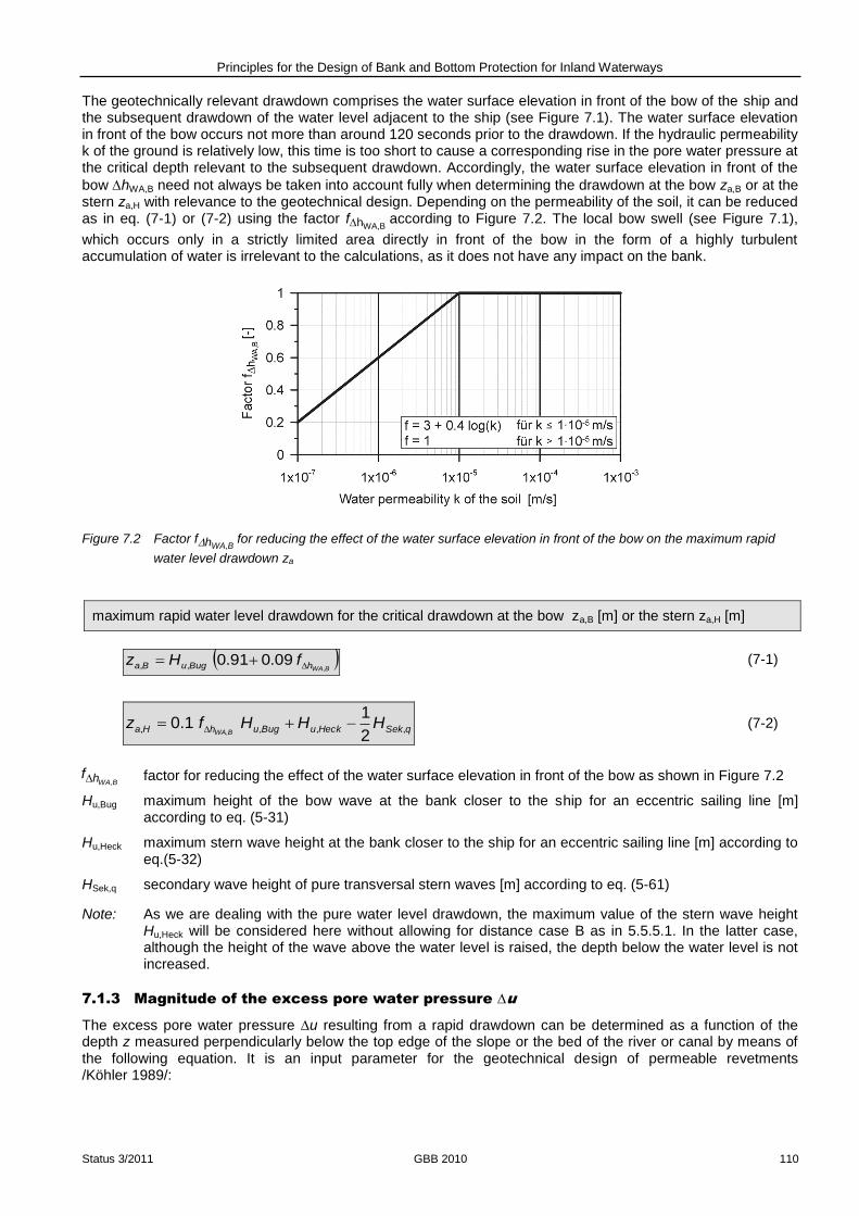
Principles for the Design of Bank and Bottom Protection for Inland Waterways
Status 3/2011 GBB 2010 110
The geotechnically relevant drawdown comprises the water surface elevation in front of the bow of the ship and the subsequent drawdown of the water level adjacent to the ship (see Figure 7.1). The water surface elevation in front of the bow occurs not more than around 120 seconds prior to the drawdown. If the hydraulic permeability k of the ground is relatively low, this time is too short to cause a corresponding rise in the pore water pressure at the critical depth relevant to the subsequent drawdown. Accordingly, the water surface elevation in front of the
bow hWA,B need not always be taken into account fully when determining the drawdown at the bow za,B or at the stern za,H with relevance to the geotechnical design. Depending on the permeability of the soil, it can be reduced as in eq. (7-1) or (7-2) using the factor fhWA,B
according to Figure 7.2. The local bow swell (see Figure 7.1),
which occurs only in a strictly limited area directly in front of the bow in the form of a highly turbulent accumulation of water is irrelevant to the calculations, as it does not have any impact on the bank.
Figure 7.2 Factor fhWA,B for reducing the effect of the water surface elevation in front of the bow on the maximum rapid
water level drawdown za
maximum rapid water level drawdown for the critical drawdown at the bow za,B [m] or the stern za,H [m]
BWAhBuguBa fHz
,09.091.0,, (7-1)
qSekHeckuBuguhHa HHHfzBWA ,,,,
2
11.0
,
(7-2)
factor for reducing the effect of the water surface elevation in front of the bow as shown in Figure 7.2
Hu,Bug maximum height of the bow wave at the bank closer to the ship for an eccentric sailing line [m] according to eq. (5-31)
Hu,Heck maximum stern wave height at the bank closer to the ship for an eccentric sailing line [m] according to eq.(5-32)
HSek,q secondary wave height of pure transversal stern waves [m] according to eq. (5-61)
Note: As we are dealing with the pure water level drawdown, the maximum value of the stern wave height Hu,Heck will be considered here without allowing for distance case B as in 5.5.5.1. In the latter case, although the height of the wave above the water level is raised, the depth below the water level is not increased.
7.1.3 Magnitude of the excess pore water pressure u
The excess pore water pressure u resulting from a rapid drawdown can be determined as a function of the depth z measured perpendicularly below the top edge of the slope or the bed of the river or canal by means of the following equation. It is an input parameter for the geotechnical design of permeable revetments /Köhler 1989/:
B,WAhf

Principles for the Design of Bank and Bottom Protection for Inland Waterways
Status 3/2011 GBB 2010 111
excess pore water pressure u [kN/m2]
zbazzu e1aW (7-3)
where
a is the pore water pressure parameter [-], a = 1,
Note: Other values may result from the mathematical description of measurement results.
b is the pore water pressure parameter [1/m] according to eq. (7-4)
e is Euler’s constant [-], e 2.718
z is the depth below the surface of the slope [m] or below the bed of the river or canal, perpendicular to the bed
za is the maximum rapid drawdown [m]
za = za,B maximum rapid drawdown for the critical drawdown at the bow as in eq.(7-1)
za = za,H maximum rapid drawdown for the critical drawdown at the stern as in eq.(7-2)
ta is the drawdown time in seconds [s] associated with za :
ta = ta,B for drawdown at the bow according to eqs. (5-47) and (5-50)
ta = ta,H for drawdown at the stern according to eq. (5-52)
ta = ta,B,Sek for secondary waves according to eq. (5-51)
W is the weight density of the water [kN/m3], W = W g
W is the density of the water [kg/m3]
The pore water pressure parameter b is a measurement for the decrease in the excess pore water pressure u with the depth.
The larger b is, the greater is the excess pore water pressure u in the subsoil and the greater is its destabilising effect on the revetment.
The pore water pressure parameter b can be determined as a function of the hydraulic permeability k of the soil for a drawdown time ta = ta* = 5 s according to Figure 7.3 or eq. (7-5). This value b (k,ta = 5 s) will be referred to below as b*. Other influential parameters such as the oedometer modulus of soil ES and the degree of saturation S of the soil have already been dealt with in Figure 7.3 and eq. (7-5) /Köhler 1997/.
The conversion of b* to a b for a different drawdown time ta ≠ 5 s may be carried out using the factor aa tt *:
a
a
t
tbb
(7-4)
where
b is the pore water pressure parameter [1/m]
b is the pore water pressure parameter [1/m] according to Figure 7.3 and eq. (7-5) for s5aa tt
b = 0.166 k-0.327
(7-5)
ta is the drawdown time [s]
ta = ta,B for drawdown at the bow according to eq. (5-47)
ta = ta,H for drawdown at the stern according to eq. (5-52)
k is the water permeability of the soil [m/s]
With eq. (7-4) lower b values are obtained for longer drawdown times ta > 5 s and, vice versa, higher b values are obtained for shorter drawdown times ta < 5 s than for ta = 5 s.

Principles for the Design of Bank and Bottom Protection for Inland Waterways
Status 3/2011 GBB 2010 112
Figure 7.3 Pore water pressure parameter b* as a function of the permeability of the soil k for a drawdown velocity
vza = 0.12 m/s /Köhler 1997/ or a drawdown time of s5*a t
7.2 Local stability of permeable revetments
7.2.1 General remarks
The rapid drawdown of the water level of a river or canal is always accompanied by excess pore water pressures in the soil close to the surface of the bed and banks of the canal or river (see 3.4.3).
Depending on the degree and velocity of drawdown, the following may therefore occur in the case of a permeable revetment if the weight per unit area of the revetment is not sufficiently large:
sliding along a failure surface in the ground parallel to the slope at the critical depth dkrit below the revetment or
hydrodynamic soil displacement directly below the revetment.
Geotechnical analyses for both above-mentioned types of failure must always be carried out in order to determine the required weight per unit area of permeable revetments on banks, i.e. for the assessment of local stability. Such analyses can also be used to check the local stability of natural bank slopes.
If the length of the depression caused by drawdown for short vessels is less than 30 m, then only the proof of resistance to hydrodynamic soil displacement according to 7.2.6 is mandatory. Because of the spatial impact of the unbound armour layer, the lateral shearing forces in this case are sufficient to prevent sliding failure of the armour layer. The length of the depression caused by drawdown can be estimated from the drawdown times and ship speed using eq. (7-6).
length of the depression caused by drawdown LAM [m]
LAM = ta,H vSüG (7-6)
where
vSüG is the ship speed over ground [m/s] according to eq. (5-20)
ta,B is the drawdown time for drawdown at the bow [s] according to eqs. (5-47), (5-50) and (5-51)
ta,H is the drawdown time for drawdown at the stern [s] according to eq. (5-52)

Principles for the Design of Bank and Bottom Protection for Inland Waterways
Status 3/2011 GBB 2010 113
7.2.2 Guidance on properties of the ground
For determining the necessary armour layer thickness, not only is the shear strength, but also the permeability of the soil of particular importance. The less permeable the natural soil is, the greater the excess pore water pressure will be at a specific hydraulic load. For a conservative estimate, the water permeability is thus to be assumed at the lower end of the possible range of values (= lowest permeability).
If the soil has a permanently effective cohesion even under water (c’ ≥ Δu tan β) as defined in Section 7.2.5.2, the local stability of permeable revetments in accordance with 7.2 can normally be assumed without further verification.
If a revetment is placed on stratified ground – estimating conservatively – the stratum requiring the highest weight per unit area will determine the weight per unit area of the revetment as a whole. Soil layers with small thicknesses (≤ 1 m) can, as a general rule, be disregarded. If significantly differing friction parameters or permeability coefficients are present, then a shear strength or permeability averaged over the slope length should be selected.
7.2.3 Depth of the critical failure surface dkrit
The shear resistance of the soil is at its lowest at the critical depth dkrit owing to the excess pore water pressure, so that, on slopes, a soil layer above the critical depth may slide. The depth of the critical failure surface is required for calculation of the required weight per unit area of the armour layer and is determined as follows:
depth of the critical failure surface dkrit [m]
0
tantancos
tanln
1 aWkrit
bz
bd (7-7)
Note: valid for ' >
where
b is the pore water pressure parameter [1/m] according to eq. (7-4)
za is the maximum rapid drawdown [m]
za = za,B maximum rapid drawdown for the relevant drawdown at the bow according to eq. (7-1) za = za,H maximum rapid drawdown for the relevant drawdown at the stern according to eq.(7-2)
is the slope angle [°]
' is the effective weight density of soil at buoyancy [kN/m³]
W is the weight density of water [kN/m3]
' is the effective angle of shearing resistance of the soil [°]
If dkrit 0, local stability is ensured even without the weight of the revetment.
Eq. (7-7) is defined only for ' > . If ≥ ', a verification with this calculation method is no longer possible. In this case, the armour layer must then be designed as if it were a retaining wall without bending stiffness.
7.2.4 Effective weight density of the armour layer at buoyancy
The effective weight density of the armour layer at buoyancy is an essential parameter for the proofs of the local stability of the revetment. It is calculated as follows:
effective weight density of the permeable armour layer at buoyancy D [kN/m³]
WSD 1 n (7-8)

Principles for the Design of Bank and Bottom Protection for Inland Waterways
Status 3/2011 GBB 2010 114
where
n is the porosity of the revetment [-]
'D is the effective weight density of the armour layer at buoyancy [kN/m³]
S is the bulk density of the armour stones [kN/m3]
W is the weight density of water [kN/m3]
For the porosity n the following values apply:
approx. 50-55% for dumping under water
approx. 45% for placing in a dry condition
approx. 30-40% for subsequent manual finishing work
These values apply assuming that the level of the tips of the armour stones is regarded as the upper edge of the armour layer. If that is the case, the values already allow for the higher porosity in the upper third of the armour layer.
7.2.5 Weight per unit area of the armour layer required to protect slope revetments
against sliding failure
7.2.5.1 General remarks
The following method of calculating the required weight per unit area of a permeable armour layer on a bank slope is based on the failure mechanisms specified for the equilibrium of forces in the plastic limit state in accordance with Rankine’s special case.
First, as a basic case, an infinitely long slope in the direction in which the slope falls is considered notionally. Then the additional influences resulting from a toe support or revetment suspension are included.
The shear stresses in the sliding surface are determined. Any other relevant forces (e.g. toe support) are converted into equivalent shear stresses.
The weight per unit area of the armour layer and the associated thickness of a permeable slope revetment are calculated for a failure surface close to the surface and parallel to the slope at the critical depth dkrit, which is
determined as described in 7.2.3.
7.2.5.2 Method of calculation
The weight of the armour layer required to prevent sliding failure of a slope is calculated according to the following equation /Köhler 1989/:
weight per unit area g' of the permeable armour layer required to prevent sliding failure [kN/m²]
)(sintancos
tankritFF
AFDD dd
cudg
(7-9)
Note: valid for ‘ >
where
c' is the effective cohesion of the soil [kN/m2]
dD is the thickness of the armour layer [m]
dF is the thickness of the filter [m]
dkrit is the critical depth of the failure surface [m] in accordance with eq. (7-7)
g' is the weight per unit area of the armour layer [kN/m2]
u is the excess pore water pressure [kN/m2] in accordance with eq. (7-3) for z = dkrit
is the slope angle [°]
' is the effective weight density of soil at buoyancy [kN/m³]

Principles for the Design of Bank and Bottom Protection for Inland Waterways
Status 3/2011 GBB 2010 115
'D is the effective weight density of the armour layer at buoyancy [kN/m³]
'F is the weight density of the filter at buoyancy [kN/m3] for geotextile filters 'F = 0
' is the effective angle of shearing resistance of the soil [°]
A is the additional stress [kN/m²] from a suspension of the armour layer (see 7.2.8)
F is the additional stress [kN/m²] from a toe support (see 7.2.7)
Eq. (7-9) is defined only for soils with an angle of shearing resistance of ' > .
If the effective cohesion c' of the natural soil is
tanuc
and if this is permanent, the safety of the revetment on a cohesive soil against sliding failure will be adequate. Permeable armour layers on a clay lining will also have an adequate level of safety against sliding failure, as the clay lining is considered as being similar to a natural cohesive soil for the purpose of the analysis.
In considering a toe support or anchoring forces, allowance is made for the resulting equivalent additional
stresses F (see 7.2.7) or A (see 7.2.8) in eq. (7-9). In this case, attention is drawn to the fact that different types
of deformation are required to mobilise these kinds of stress and that they may be allowed for only to the degree to which they are mobilised.
The required equivalent shear stress erf is obtained for a selected armour layer thickness by means of eq. (7-9) as follows:
required equivalent shear stress erf [kN/m²]
cuddd tantancossinerf kritFFDD (7-10)
where
c' is the effective cohesion of the soil [kN/m2]
dD is the thickness of the armour layer [m]
dF is the thickness of the filter [m]
dkrit is the critical depth of the failure surface [m] in accordance with eq. (7-7)
erf is the required shear stress [kN/m²]
F with a toe support
A with a revetment suspension
u is the excess pore water pressure [kN/m2] in accordance with eq. (7-3) for z = dkrit
is the slope angle [°]
' is the effective weight density of soil at buoyancy [kN/m³]
'D is the effective weight density of the armour layer at buoyancy [kN/m³]
'F is the effective weight density of the filter at buoyancy [kN/m3] for geotextile filters 'F = 0
' is the effective angle of shearing resistance of the soil [°]

Principles for the Design of Bank and Bottom Protection for Inland Waterways
Status 3/2011 GBB 2010 116
7.2.6 Weight per unit area of the armour layer required to prevent hydrodynamic soil
displacement
7.2.6.1 General remarks
If there is a high toe support force, a revetment suspension or a very gentle slope inclination, the necessary weight per unit area of the revetment required to prevent sliding failure may become so low that the excess pore water pressure may cause the surface of the soil to move upwards, resulting in a loosening of the ground.
This may result in hydrodynamic soil displacement below the revetment in non-cohesive soils (c' = 0) /Köhler, Koenders 2003/. In such a case, the weight per unit area selected for the design must be high enough to suppress the excess pore water pressure at the critical depth by applying a sufficiently high surcharge.
The above verification is not required for cohesive soils (c' > 0) as hydrodynamic soil displacement does not occur.
7.2.6.2 Method of calculation
The weight per unit area g' of the armour layer at buoyancy that is required to prevent hydrodynamic displacement of the soil is calculated as follows analogously to hydraulic heave:
weight per unit area g' of the permeable armour layer at buoyancy required to prevent hydrodynamic soil displacement [kN/m²]
)(cos
krithBFFDD ddu
dg
(7-11)
where
b is the pore water pressure parameter [1/m] according to eq. (7-4)
dD is the thickness of the armour layer [m] measured perpendicularly to the surface
dF is the thickness of the filter [m] measured perpendicularly to the surface
dkrithB is the critical depth of the failure surface [m] relevant to the hydrodynamic displacement of soil
0bz
b
1d aw
krithB
cosln (7-12)
g ' is the weight per unit area of the armour layer [kN/m2]
za is the maximum rapid drawdown [m], see 7.1.2
is the slope angle [°]
'D is the effective weight density of the armour layer at buoyancy [kN/m³]
' is the effective weight density of soil at buoyancy [kN/m³]
'F is the effective weight density of the filter at buoyancy [kN/m3] for geotextile filters 'F = 0
W is the weight density of water [kN/m3]
u is the excess pore water pressure [kN/m2] in accordance with eq. (7-3) for z = dkrit
7.2.7 Weight per unit area of an armour layer taking into account a toe support
7.2.7.1 General remarks
If the revetment at the toe of the slope is designed as specified in /MAR 2008/ (e.g. with a toe blanket, embedded toe or sheet pile wall at the toe), a toe support force can be taken into consideration when determining the weight per unit area of the armour layer. The magnitude of the toe support force results from the shear strength of the revetment (failure mechanism 1) or from the stability of the toe of the revetment (failure mechanism 2).

Principles for the Design of Bank and Bottom Protection for Inland Waterways
Status 3/2011 GBB 2010 117
The method of calculating the mobilisable toe support force is based on conservative simplifications of the failure geometry and the shear resistance. The toe support force is considered as an equivalent shear stress in the sliding surface.
Generally speaking, two failure mechanisms of the supported revetment may occur in a slope:
Failure mechanism 1: The revetment shears off in a horizontal joint through the upper edge of the toe of the revetment (see Figure 7.4).
Failure mechanism 2: Failure of the toe of the revetment (see Figures 7.5, 7.6 and 7.7).
The failure mechanism for which the higher armour layer weight is obtained is decisive for the design and depends on the design of the toe of the revetment.
7.2.7.2 Failure mechanism 1 at the upper edge of the toe of the revetment
In the case of failure mechanism 1, the sliding surface is located at the upper edge of the toe of the revetment and passes horizontally through the revetment (Figure 7.4). This failure mechanism does not depend on the design of the toe.
Figure 7.4 Failure mechanism 1 of a toe support
The equivalent shear stress max F1 resulting from the toe support force below the slope revetment cannot exceed the value required for equilibrium in the direction in which the slope falls.
The required weight per unit area g' of the armour layer or the associated armour layer thickness is obtained for failure mechanism 1 as follows:
required thickness of the permeable armour layer dD for failure mechanism 1 [m]
AC
BAd
D
2D
5.0 (7-13)
with the auxiliary functions
A = (C 'D dF - D E 'D) / C 'D
B = D E (dF 'F + dkrit ´) + D F - G
C = tan'D cos
D = (cos - sin tan'D) (hW - za)
E = sin - cos tan'
F = u tan' - c‘
G = 0.5 dF2 'F

Principles for the Design of Bank and Bottom Protection for Inland Waterways
Status 3/2011 GBB 2010 118
and with the symbols
c' effective cohesion of the soil [kN/m2]
dF thickness of the filter [m]
dkrit critical depth of the failure surface [m] in accordance with eq. (7-7)
hW water depth at still water level [m]
za maximum rapid drawdown [m], see 7.1.2
slope angle [°]
'D effective weight density of the armour layer at buoyancy [kN/m³]
'F effective weight density of the filter at buoyancy [kN/m3] for geotextile filters 'F = 0
' effective weight density of soil at buoyancy [kN/m³]
' effective angle of shearing resistance of the soil [°]
'D effective angle of shearing resistance of the armour layer material [°] in ungrouted armour layers 'D = 55°
u excess pore water pressure [kN/m2] in accordance with eq. (7-3) for z = dkrit
The maximum equivalent shear stress max F1 due to shearing in the revetment in the direction in which the slope falls is obtained as follows:
maximum equivalent shear stress max F1 for failure mechanism 1 [kN/m²]
awD
DD2
DFDF2
F
F1tansincos
costan2
1
2
1
maxzh
dddd
(7-14)
where
dD is the thickness of the armour layer [m]
dF is the thickness of the filter layer [m]
hw is the water depth at still water level [m]
za is the maximum rapid drawdown [m], see 7.1.2
is the slope angle [°]
'D is the effective weight density of the armour layer at buoyancy [kN/m³]
'F is the effective weight density of the filter at buoyancy [kN/m³]
'D is the angle of shearing resistance of the armour layer material [°] in ungrouted armour layers 'D = 55°
max F1 is the maximum possible equivalent shear stress [kN/m2] below the slope revetment for failure
mechanism 1
7.2.7.3 Failure mechanism 2 with a toe blanket
If a toe blanket is used, the critical sliding surface in failure mechanism 2 will occur underneath the filter layer, following the boundary between the subsoil and the toe blanket, wedging out below the passive earth pressure wedge in front of the toe blanket at the level of the bed of the river or canal (see Figure 7.5). Beneath the slope, the critical sliding surface runs as in failure mechanism 1 (see 7.2.7.2).

Principles for the Design of Bank and Bottom Protection for Inland Waterways
Status 3/2011 GBB 2010 119
Figure 7.5 Failure mechanism 2 in a slope revetment with a toe blanket
The excess pore water pressure in the bed of the river or canal caused by drawdown za (see 7.1) generates an unsteady upward flow of pore water that can temporarily destabilise the soil at the bed. The flow results in the loss of the effective stress of the soil at the bed above the critical depth tkrit immediately after the maximum drawdown za has been reached. Consequently, there is a reduction in the supporting effect of the mobilisable passive earth pressure in front of the toe blanket /Köhler, Koenders 2003/. The difference between the vertical
stress from the potentially buoyant soil block G' (see Annex A) and the excess pore water pressure u(z) at the bed, which varies with time, results in a minimum in the critical depth tkrit. The surplus energy from the unsteady pore water flow is dissipated by the incipient vertical soil movement.
This critical depth tkrit at the bed (from eq. (7-7) for the slope angle = 0) is calculated as follows:
0'
ln1 aW
krit
zb
bt (7-15)
The maximum equivalent shear stress max F2 that can be assumed for the toe blanket is calculated from the required equilibrium conditions (see Annex A) of all forces acting inside and outside of the toe of the revetment (cf. Figure 7.5), where the following applies:
maximum equivalent shear stress max F2 for failure mechanism 2 for a toe blanket [kN/m²]
)z(h
dddd
awDFDFDF
DFFFDFFF2
FFDF
2
DF
iF2,tan2sincotcos
sin2
max
inside (7-16)
aw
phFuv
aF2,'tansincos
sin'''tan'max
zh
ELc
outside (7-17)
with the equation
FFFFDFDFv dd (7-18)
and with the symbols
b pore water pressure parameter [1/m] according to eq. (7-4)
c' effective cohesion of the soil [kN/m2]
dDF thickness of the armour stone layer in the toe blanket [m]
dFF thickness of the filter in the toe blanket [m]
E'ph horizontal component of the passive earth pressure in front of the toe blanket [kN/m] according to eq. (7-21)
hW water depth at still water level [m]

Principles for the Design of Bank and Bottom Protection for Inland Waterways
Status 3/2011 GBB 2010 120
LFu length of the toe blanket [m]
max F2 maximum equivalent shear stress [kN/m2] below the slope revetment due to the toe blanket
tkrit critical depth at the river or canal bed [m]
tF thickness of the toe blanket as a whole [m]
za maximum rapid drawdown [m], see 7.1.2
slope angle [°]
' effective weight density of soil at buoyancy [kN/m³]
'DF effective weight density of the armour layer in the toe blanket at buoyancy [kN/m³]
'FF effective weight density of the granular filter in the toe blanket at buoyancy [kN/m3]; for geotextile filters in
the toe blanket: 'FF = 0
W weight density of water [kN/m3]
DF angle of the sliding surface of the passive earth pressure wedge within the toe blanket [° ] , 35DF
p angle of sliding surface of the passive earth pressure wedge in the soil directly in front of the toe blanket [°]
'v effective vertical stress [kN/m²]
' effective angle of shearing resistance of the soil [°]
'DF effective angle of shearing resistance of the riprap in the toe blanket [°], 'DF ≤ 35°
The approach using earth pressure for toe support force is only permissible if scouring in front of the toe blanket can be ruled out. Otherwise the earth pressure E'ph must not be included in eq. (7-17).
For assessments of the internal, maximum shear stress max F2,i that can be mobilized if a toe support is used,
the angle of shearing resistance 'DF must be limited to 'DF = 35°, as larger angles of shearing resistance will
lead to incorrect results being obtained when using the algorithms for rigid failure mechansims to calculate the internal shear stress.
The thickness tF = dDF + dFF and the length LFu of the toe blanket must first be specified. The dimensions finally selected for the toe blanket must satisfy the following three conditions:
(1) The safety against liquefaction of the soil for the selected thickness tF must be verified in order to ensure a sufficient minimum thickness of the toe blanket. The following inequality must be satisfied, while taking into
consideration the critical depth t krit below the river or canal bed ( = 0):
DF
kritFFFFaWDF
krit1
tdez
d
tb
(7-19)
The required minimum thickness of the armour layer dDF must satisfy the above inequality for the selected thickness tF of the toe blanket. If in a location with stratified ground the type of natural soil present in the vicinity of the toe of the slope differs from that at the slope itself, then the permeability of the soil at the toe of the slope should be used for determining b according to eq.(7-4) and tkrit according to eq. (7-15).
(2)The length LFu of the toe blanket, which is to be specified, must be determined in such a way that it does not exceed the maximum permissible length (max LFu) and that it ensures the minimum length (min LFu ) required for inner stability.
The following applies to the final specification of the length LFu of the toe blanket:

Principles for the Design of Bank and Bottom Protection for Inland Waterways
Status 3/2011 GBB 2010 121
min LFu LFu max LFu
FFu 4max tL (7-20)
DF
FFu
tanmin
tL
with the simplifying and conservative assumption for determining the passive sliding surface angle DF at the
passive earth pressure wedge within the toe blanket (verification of internal shear stress):
35DF
(3) The relevant angle of shearing resistance ' of the soil at a bed of the river or canal is used to calculate the passive earth pressure in front of the toe blanket E'ph as follows
pppvph costansin CCUGE (7-21)
with the auxiliary functions
p
2
kritF
2
ttG
tan
and
245p
p
kritF ttcC
sin
kritFp
awv
krit
kritF
tantte
b
eezU
tbtbtb
N.B.: excess pore water pressure Uv applies only when Uv 0; when Uv < 0 use Uv = 0
and with the symbols
b pore water pressure parameter [1/m] according to eq. (7-4)
c' effective cohesion of the soil [kN/m2]
E'ph horizontal component of the passive earth pressure in front of the toe blanket [kN/m]
tkrit critical depth at the river or canal bed [m]
tF thickness of the toe blanket as a whole [m]
za maximum rapid drawdown [m], see 7.1.2
W weight density of water [kN/m3]
' effective weight density of soil at buoyancy [kN/m³]
' effective angle of shearing resistance of the soil [°]
p angle of sliding surface of the passive earth pressure wedge in the soil directly in front of the toe blanket [°]
The maximum equivalent shear stress max F2 that can be transmitted by the toe blanket is obtained by comparing the results for the external and internal shear stresses obtained in accordance with eqs. (7-16) and (7-17). The lower of the two calculated shear stress values shall be the one used in the following calculation of the required weight per unit area g' of the armour layer on the slope.
required weight per unit area of a permeable armour layer g' for designs including a toe blanket [kN/m2]
kritFF
F2DD
sintancos
maxtandd
cudg (7-22)

Principles for the Design of Bank and Bottom Protection for Inland Waterways
Status 3/2011 GBB 2010 122
where
c' is the effective cohesion of the soil [kN/m2]
dD is the thickness of the armour layer [m]
dF is the thickness of the filter [m]
dkrit is the critical depth of the failure surface [m] in accordance with eq. (7-7)
g' is the required weight per unit area [kN/m²] of the armour layer for failure mechanism 2
max F2 is the maximum equivalent shear stress [kN/m²] from the toe blanket for failure mechanism 2:
for minimum, see eqs. (7-16) and (7-17)
u is the excess pore water pressure [kN/m2] in accordance with eq. (7-3) for z = dkrit
za is the maximum rapid drawdown [m], see 7.1.2
is the slope angle [°]
' is the effective weight density of soil at buoyancy [kN/m³]
'D is the effective weight density of the armour layer at buoyancy [kN/m³]
'F is the effective weight density of the filter at buoyancy [kN/m3] for geotextile filters 'F = 0
' is the effective angle of shearing resistance of the soil [°]
7.2.7.4 Failure mechanism 2 for an embedded toe
In failure mechanism 2 for an embedded toe, a sliding surface will be examined which runs under the slope at a distance dkrit from the boundary between filter and soil, in the area of the embedded toe directly along the boundary filter/soil and in the soil under the waterway bed underneath the passive soil wedge (see Figure 7.6).
The excess pore water pressure is also relevant to the revetment at the embedded toe below the bed of the river or canal as the pores in this area may be clogged with backfill. The permeability of the latter will then be relevant to the revetment too.
The rapid drawdown also generates excess pore water pressure in the soil at the horizontal bed (see 7.1) and, consequently, a pore water flow. The pore water flow leads to a loss of the effective stresses (soil liquefaction) near the surface reaching to the critical depth tkrit. At the depth tkrit the buoyant force resulting from the difference between the excess pore water pressure and the vertical stress due to the dead weight of the soil reaches its maximum value. The energy arising from the pore water flow is dissipated by the movement of the soil. The
critical depth tkrit at the river or canal bed (slope angle = 0) is calculated analogously to eq. (7-15) as follows:
0ln1 aW
krit
zb
bt (7-23)
Figure 7.6 Failure mechanism 2 for a bank revetment with an embedded toe
The maximum equivalent shear stress max F2 is calculated from the equilibrium conditions for the sliding
wedge shown in Figure 7.6.

Principles for the Design of Bank and Bottom Protection for Inland Waterways
Status 3/2011 GBB 2010 123
maximum equivalent shear stress max F2 for failure mechanism 2 for an embedded toe [kN/m²]
22v211v1
F2
kritkaWu
u
F2F2
sin
0max
CD
GU
B
ACGUF
ttzhL
L
F
(7-24)
with the auxiliary functions
cotcossin
cotcossin
cotcossin
p
ppp
D
B
A
kritFaW
v2
kritFp
aWv1
krit
kritF
krit
kritF
tan
tan
tteb
eezU
tteb
eezU
tbtbtb
tbtbtb
tantantan
tan)tan1(arctan
sin;
sin
tan2;
tan2
2
p
kritF2
p
kritF1
2kritF
2p
2kritF
1
ttcC
ttcC
ttG
ttG
and with the symbols
see below eq. (7-25).
The weight per unit area required in this case is then obtained as follows, taking into account the maximum attainable equivalent shear stress:
required weight per unit area of the permeable armour layer g' for designs including an embedded toe [kN/m²]
kritFFF2
DD
sintancos
maxtandd
cu
dg
(7-25)
where
b is the pore water pressure parameter [1/m] according to eq. (7-4)
c' is the effective cohesion of the soil [kN/m2]
dD is the thickness of the armour layer [m]
dF is the thickness of the filter [m]
dkrit is the critical depth within the slope [m] in accordance with eq. (7-7)
hW is the water depth at still water level [m]
tF is the depth of the toe embedment [m]

Principles for the Design of Bank and Bottom Protection for Inland Waterways
Status 3/2011 GBB 2010 124
tk is the scour depth at the river or canal bed in front of the toe of the revetment [m]
tkrit is the critical depth at the bed [m] according to eq. (7-23)
u is the excess pore water pressure [kN/m2] in accordance with eq. (7-3) for z = dkrit
za is the maximum rapid drawdown [m], see 7.1.2
is the slope angle [°]
' is the effective weight density of the soil at buoyancy [kN/m³]
'D is the effective weight density of the armour layer at buoyancy [kN/m³]
'F is the effective weight density of the filter at buoyancy [kN/m³]
W is the weight density of water [kN/m3]
' is the effective angle of shearing resistance of the soil [°]
p is the angle of the sliding surface [°]
max F2 is the maximum equivalent shear stress due to the embedded toe [kN/m²] according to eq. (7-24)
Depending on local experience, scouring to a depth of tk may need to be taken into consideration as in Figure 7.6 when specifying the embedment depth tF.
Negative values may be obtained when determining the required thickness of the armour layer dD. In this event,
a revetment is not required for the assessment of the toe embedment. The thickness of the revetment is then obtained using failure mechanism 1.
7.2.7.5 Failure mechanism 2 for a sheet pile wall at the toe
Failure mechanism 2 consists of the failure of a fixed sheet pile wall installed at the lower edge of a slope revetment. The following influences must be taken into consideration when designing sheet pile walls (see Figure 7.7):
(a) the toe support force F acting on the head of the sheet pile wall in the direction in which the armour layer
falls; F is obtained from the additional shear stress erf F according to eq. (7-10) for the selected thickness
dD of the armour layer in conjunction with the following equation:
uFerf LF (7-26)
where
hW is the water depth at still water level [m]
Lu is the length of the slope revetment below the water level [m]
sin
aWu
zhL
(7-27)
za is the maximum rapid drawdown [m], see 7.1.2
is the slope angle [°]
erf F is the required shear stress for a sheet pile wall at the toe [kN/m²] according to eq. (7-10)
(b) the active earth pressure E'a in the soil below the slope revetment
(c) a scour depth tk, to be specified in accordance with /MAR 2008/ or according to experience with local conditions
(d) the critical depth tkrit, at which the buoyancy force due to the difference between the excess pore water pressure and the self-weight of the soil reaches its maximum
(e) the excess pore water pressure resulting from excess pore water pressure at both sides Ub = u(tk) where tk > 0 according to Figure 7.7.

Principles for the Design of Bank and Bottom Protection for Inland Waterways
Status 3/2011 GBB 2010 125
Figure 7.7 Toe support for a slope revetment in the form of a sheet pile wall (failure mechanism 2)
Symbols: E'a - active earth pressure, E'p - passive earth pressure, F - force from the revetment, tk – scour depth, Ub - resultant force of excess pore water pressure
Unanchored sheet pile walls are designed for full restraint in accordance with /EAU 2004/. If a scour depth tk is assumed, the stress assessment for the load case 2 /EAU 2004/ is to be carried out if the scour is of only temporary duration.
The excess pore water pressure at the bed must be taken into account when determining the earth resistance E'p in front of the sheet pile wall analogously to eq. (7-3). E'p is the resultant of the earth resistance inclined at a
wall friction angle p = 2/3 ' in accordance with /DIN 4085/.
A simplified, conservative, method for determining the values of the horizontal earth pressure force E'ph can be carried out using the earth pressure ordinates e'ph according to the equation stated below, which includes the effect of the excess pore water pressure due to rapid drawdown. The passive earth pressure can be taken as increasing linearly with the depth (see Figure 7.7).
earth pressure ordinate e'ph (tF) [kN/m²]
kritF
pp
Fph
cos2
tt
Ete
(7-28)
with the auxiliary functions
p
2
kritF
p
kritF
ppp
pppv
p
tan2
sin
cotcossin
sincotcos
ttG
ttcC
CGUE
kritFp
awv
krit
kritF
tantte
b
eezU
btbtbt

Principles for the Design of Bank and Bottom Protection for Inland Waterways
Status 3/2011 GBB 2010 126
bz
bt
)(
aWkrit
p
2
p
ln1
tantantan
tantan1arctan
and with the symbols
b pore water pressure parameter [1/m] according to eq. (7-4)
c' effective cohesion of the soil [kN/m2]
E'p passive earth pressure [kN/m]
t depth below the bed of the river or canal [m]
tkrit critical depth [m] at the river or canal bed (= 0°) according to eq.(7-23)
tF depth of the sheet pile wall at the toe [m] (the selected value of tF must be greater than tkrit)
za maximum rapid drawdown [m], see 7.1.2
' effective weight density of soil at buoyancy [kN/m³]
p wall friction angle [°]; as a rule p = 2/3 ' for sheet pile walls
W weight density of water [kN/m3]
' effective angle of shearing resistance of the soil [°]
p angle of the sliding surface [°]
The vertical component of the excess pore water pressure u in the area of earth resistance is already included in eq. (7-28).
The active earth pressure E'a may be determined using the effective weight density of the soil at buoyancy in accordance with /DIN 4085/.
The resulting water pressure on the active side may be simplified by means of a triangle, as shown in Figure 7.7, of which the ordinate is obtained at the lower edge of the scour using eq. (7-3) for the depth
z = t k = tk - (dF+dD)/cos and for the drawdown time t = ta .
The stability of the armour layer is guaranteed if the sheet pile wall at the toe can be dimensioned for the influences referred to in (a) to (c). The weight of the armour layer or the embedment depth and, if applicable, the moment of resistance of the sheet piles must otherwise be increased.
7.2.8 Weight per unit area of the armour layer allowing for a suspension of the revetment
7.2.8.1 General remarks
The stability of the revetment can be increased by anchoring the armour layer at the top (“suspended revetment”) as in Figure 7.8. These kinds of suspension can either consist of individual anchors (steel cables, high-tensile fabric strips) or high-tensile sheets (geosynthetics).
The use of a suspension (= anchor) in conjunction with other supporting construction components (such as a toe support) means the latter cannot be presumed for purposes of statics because of their differing mobilisation behaviour.
The tensile force Z that must be withstood is obtained by multiplying the required shear stress erf according to eq. (7-10) depending on the selected thickness of the revetment dD, by the length Lu of the armour layer lying
below the lowered water level.
The following verifications must be performed if the resistance to the tensile force Z is to be provided by the weight of the armour layer above the lowered water level:
verification of the external load-bearing capacity (see 7.2.8.2)
verification of the internal load-bearing capacity (see 7.2.8.3)

Principles for the Design of Bank and Bottom Protection for Inland Waterways
Status 3/2011 GBB 2010 127
Figure 7.8 Diagram showing a method for the suspension of a slope revetment
7.2.8.2 Verification of the external local-bearing capacity
The external load-bearing capacity should be verified as described below if the anchoring forces above the lowered water level are transferred into the ground by friction below the armour layer. The required weight per unit area g' of the armour layer is obtained as follows:
required weight per unit area g' of a permeable armour layer, taking into account the suspension of the revetment [kN/m²]
FoFo
ABo
ABoABABDoDo d
L
LcZdg
sin
coscos (7-29)
with the quantities
uAerf LZ (7-30)
sin
kWu
tzhL a
(7-31)
and with the symbols
c'AB cohesion/adhesion between tension element and soil above the lowered water level [kN/m²]
Note: Without verification assume c'AB = 0.
dDo thickness of the armour layer above the lowered water level [m]
dFo thickness of a mineral filter above the lowered water level [m]
erf A required additional supporting shear stress [kN/m²], erf A = erf according to eq. (7-10)
Lu length of the slope revetment below the lowered water level [m]
Lo length of the slope revetment above the lowered water level [m]
hW water depth at still water level [m]
tk depth of scour at the bed in front of the toe of the revetment [m], to be determined according to experience of local conditions
za maximum rapid drawdown [m], see 7.1.2
Z tensile force of a revetment suspension [kN/m]
slope angle [°]

Principles for the Design of Bank and Bottom Protection for Inland Waterways
Status 3/2011 GBB 2010 128
Do weight density of the armour layer above the lowered water level [kN/m3]
Fo weight density of a mineral filter above the lowered water level [kN/m³]
'AB effective angle of shearing resistance [°] between tension element and soil or between tension element
and armour layer above the lowered water level, whichever is smaller
Forms of load transfer other than by friction in the revetment (e.g. anchor trenches) must be assessed separately in respect of the tensile force Z.
7.2.8.3 Verification of the internal load-bearing capacity
The internal load-bearing capacity of the anchorage is to be verified in accordance with the methods of designing reinforcement elements, e.g. stress analysis or limit state GZ 1B in accordance with the safety concept involving partial safety factors as described in sub-clause 4.3.2 of /DIN 1054/. The strain under service load of geosynthetics may not exceed 2% of the strain at failure as specified in /DIN EN ISO 10319/.
If the resulting thickness dDo of the armour layer above the lowered water level is too large, the weight per unit area of the armour layer dD below the lowered water level can be increased to reduce the tensile force that is transmitted. If permitted by the verification of the internal load-bearing capacity, the tension elements can be anchored in a trench at the shoulder of the embankment slope in accordance with the Empfehlungen für den Entwurf und die Berechnung von Erdkörpern mit Bewehrungen aus Geokunststoffen (Recommendations for Design and Analysis of Earth Structures using Geosynthetic Reinforcements) /EBGEO 1997/.
7.2.9 Slope revetment above the lowered water level
The stability of a slope above the lowered water level is ensured if the revetment required to protect the slope from erosion extends to the highest wave run-up point in accordance with 5.5.5.5.
If, in a slope which is in a stationary state, groundwater seeps from a position above the slope revetment, the local stability of the part of the slope parallel to the surface that is fully subject to seepage is ensured according to /DIN 4084/, issue 2009, provided that the unprotected slope of non-cohesive material satisfies the following condition :
tan
'
'tan
W
(7-32)
where
is the slope angle above the lowered water level [°]
' is the effective weight density of soil at buoyancy [kN/m³]
W is the weight density of water [kN/m3]
' is the effective angle of shearing resistance of the soil [°]
Assuming that the weight density of the soil at buoyancy is equal to the density of water, the following simplification can be used (see 3.5):
2
(7-33)
If this condition is not satisfied and if it is not intended to extend the slope revetment over the area in which groundwater seepage occurs, other suitable measures will be required to prevent damage.
As a general rule cohesive soils are stable in this respect.

Principles for the Design of Bank and Bottom Protection for Inland Waterways
Status 3/2011 GBB 2010 129
7.3 Local stability of impermeable revetments
7.3.1 General remarks
The impermeable revetment must be designed to withstand the maximum excess water pressure if the ground water level is sometimes higher than the lowered water level in the canal.
The weight per unit area of the armour layer of an impermeable revetment must be large enough to prevent uplift of the revetment caused by the excess pressure below the lining (see 7.3.2).
If the impermable revetment is constructed without a toe support, an additional verification of resistance to sliding (see 7.3.3) must be carried out.
7.3.2 Weight per unit area of the armour layer of an impermeable revetment to resist
uplift
In the case of an impermeable revetment on the bed or of an impermeable revetment on a slope with adequate toe support it must be verified that the weight per unit area of the revetment is sufficient to resist uplift.
The weight per unit area g' of the armour layer of an impermeable revetment required to resist uplift is calculated as:
weight per unit area g' of the armour layer of an impermeable revetment required to resist uplift [kN/m²]
)(cos
DiDiFFA
DD ddu
dg
(7-34)
with the equation
WaW )( zhu (7-35)
and with the symbols
dD thickness of the armour layer [m]
dDi thickness of the impervious lining [m]
dF thickness of the filter [m]
g ' weight per unit area of the armour layer [kN/m2]
u excess pore water pressure below the lining [kN/m²]
za maximum rapid drawdown [m], see 7.1.2
slope angle [°]
hW height difference [m] between the groundwater level and still water level of the waterway:
when the groundwater level is higher than the still water level this value is positive
A safety against uplift [-], A = 1.00
'D effective weight density of the armour layer at buoyancy [kN/m³]
'Di effective weight density of the lining material at buoyancy [kN/m³]
'F effective weight density of the filter at buoyancy [kN/m³]
7.3.3 Weight per unit area of the armour layer of an impermeable revetment without toe
support required to resist sliding
The weight per unit area of the armour layer of an impermeable slope revetment without any additional support necessary to resist sliding at the boundary surface between lining and soil is calculated as follows:

Principles for the Design of Bank and Bottom Protection for Inland Waterways
Status 3/2011 GBB 2010 130
weight per unit area g' of the armour layer of an impermeable revetment required to resist sliding [kN/m²]
)(sintancos
tanDiDiFFDD dd
cudg
(7-36)
where
c' is the effective cohesion of the soil [kN/m2]
dD is the thickness of the armour layer [m]
dDi is the thickness of the impervious lining [m]
dF is the thickness of the filter [m]
g' is the weight per unit area of the armour layer [kN/m2]
u is the excess pore water pressure below the lining [kN/m²] according to eq. (7-35)
za is the maximum rapid drawdown [m], see 7.1.2
is the slope angle [°]
hW is the height difference [m] between the groundwater level and still water level of the waterway:
when the groundwater level is higher than the still water level this value is positive
'D is the effective weight density of the armour layer at buoyancy [kN/m³]
'Di is the effective weight density of the lining material at buoyancy [kN/m³]
'F is the effective weight density of the filter at buoyancy [kN/m³]
W is the weight density of water [kN/m3]
' is the effective angle of shearing resistance of the soil [°]
The verification of a failure surface in the lining when assuming the strength of the lining as the undrained shear strength cu ≥ 5 kN/m², in comparison with eq. (7-36), leads to a smaller thickness of the armour layer. A verification of sliding in the lining is therefore not generally required.
7.4 Verification of the global stability of the water-slide slope
The global stability of the water-side slope must be verified according to /DIN 1054/ for the limit state GZ 1C with the method specified in /DIN 4084/. The following situations are to be examined:
(a) operating water level BW or mean water level MW without drawdown with the partial safety factors for load case LC 1 according to /DIN 1054/
(b) water level drawdown as a result of the passage of a ship, assuming stationary pore water pressure that is, without allowing for the excess pore water pressure as described in 7.1 with the partial safety factors for load case LC 2 according to /DIN 1054/; the stationary pore water pressure can be assumed, for example, as drawdown acting
- as hydrostatic excess pressure on the sliding body or
- via a seepage line, which is formed by the existing initial water level in the soil and the lowered water level in the waterway and runs between the two on the slope below the revetment
N.B.: The excess pore water pressures according to 7.1 can be disregarded here for the verification of the global stability, as their destabilising effect on the large failure bodies that are critical to the global stability is significantly less than on the relatively small and flat failure bodies that are of importance when verifying the local stability as in 7.2, 7.3 and Chapter 8.
Critical high water levels in impounded or free-flowing waterways and the associated load case are to be defined for each specific case and, where appropriate, the rapidly receding flood wave should also be considered.
On operational traffic routes possible load from traffic is to be allowed for.

Principles for the Design of Bank and Bottom Protection for Inland Waterways
Status 3/2011 GBB 2010 131
8 Hydraulic and geotechnical design of armour layers consisting of
partially grouted armour stones
8.1 Hydraulic Design
Field tests and experience have shown that partially grouted armour layers as specified in /MAV 1990/ provide adequate resistance to all known hydraulic actions occurring on waterways. Hydraulic design is not then required, provided that the maximum flow velocity does not exceed 7.7 m/s /LWI 1998/, which is generally the case.
Experience has shown that adequate safety against damage caused by anchor cast and furrowing on inland waterways is ensured when the armour layer is at least 40 cm deep, and the quantity of grout is selected as specified in /MAV 1990/.
8.2 Geotechnical Design
8.2.1 General remarks
For the sake of simplification, the design may be calculated with an angle of shearing resistance of 'D = 70° for
the overall shear strength for a partially grouted armour layer in accordance with /MAV 1990/. The quantity of grouting material can be included in the calculation of the weight density of the revetment as follows:
mass per unit area of a partially grouted armour layer at buoyancy g ' [kN/m²]
WVV
DWS1000
1 m
dng (8-1)
where
dD is the thickness of the armour layer [m]
g ' is the mass per unit area of a partially grouted armour layer at buoyancy [kN/m²]
mV is the quantity of grouting material used [l/m²]
N.B.: denominator of 1000 due to conversion of litres to cubic metres
n is the voids ratio of the ungrouted armour layer [-] in accordance with 7.2.4
S is the bulk density of the armour stones [kN/m3]
V is the weight density of the grouting material [kN/m³], as a rule V = 22 kN/m³
W is the weight density of water [kN/m3]
8.2.2 Local stability of permeable revetments with partially grouted armour layers
For the geotechnical design of partially grouted armour layers it must be verified that
- adequate safety against hydrodynamic soil displacement beneath the revetment is ensured as specified in 7.2.6 and
- adequate safety of the slope above the revetment is ensured as specified in 7.2.9.
Note: The extent of dynamic hydraulic actions on armour layers due to the passage of ships is limited. The internal bond of partially grouted armour layers is sufficient to transfer forces to lateral areas not subject to load. Consequently, verification that the armour layer provides safety against sliding and shearing is not required.
An embedded toe (toe extension as described in /MAR 2008/) is generally required to provide protection against scour.

Principles for the Design of Bank and Bottom Protection for Inland Waterways
Status 3/2011 GBB 2010 132
8.2.3 Local stability of impermeable revetments with partially grouted armour layers
For the geotechnical design of partially grouted armour layers above an impervious lining it must be verified that
- adequate safety against uplift of the revetment is ensured according to 7.3.2 and
- adequate safety against sliding of the revetment on the slope is ensured according to 7.3.3.
8.3 Verification of the global stability of the water-side slope
The global stability of the slope must be verified as specified in 7.4.

Principles for the Design of Bank and Bottom Protection for Inland Waterways
Status 3/2011 GBB 2010 133
9 Literature
/Abromeit 1997/ Abromeit, H.-U.
Ermittlung technisch gleichwertiger Deckwerke an Wasserstraßen und im Küstenbereich in Abhängigkeit von der Trockenrohdichte der verwendeten Wasserbausteine [Determination of technically equivalent revetments on waterways or in marine environment dependent on the density of armour stone used]
in: BAW Newsletter No. 75, pp. 1-76
Self-published, Karlsruhe 2004
/BAW 2005/ Bundesanstalt für Wasserbau [Federal Waterways Engineering and Research Institute]
Principles for the Design of Bank and Bottom Protection for Inland Waterways (GBB 2004) Newsletter No. 88
Self-published, Karlsruhe 2005
/BAW 2008/ Bundesanstalt für Wasserbau [Federal Waterways Engineering and Research Institute]
GBBSoft – Software for Designing Bank and Bottom Protection for Inland Waterways
Software and manual
Karlsruhe 2008
/BAW 2009/ Bundesanstalt für Wasserbau [Federal Waterways Engineering and Research Institute]
Fahrversuche am Wesel-Datteln-Kanal und Modellversuche bei der DST zur Frage der Sohlen- und Deckwerksstabilität bei Schifffahrt [Navigation trials on the Wesel-Datteln Canal and model tests at the DST regarding the staibility of bed and revetment when affected by shipping]
unpublished
/Binek, Müller 1991/ Binek, H., Müller, E.
Bestimmung der Wassertiefenabhängigkeit des Formfaktors eines Ein-Schrauben-Binnenschiffes [Determination of the dependency of the relation between water depth and form factor of a single screw inland navigation vessel]
Früher: Versuchsanstalt für Binnenschiffbau; heute: Entwicklungszentrum für Schiffstechnik und Transportsysteme e.V. [formerly: Test Centre for Inland Navigation Vessels; currently: Development Centre for Ship Technology and Transport Systems]
Self-published, Duisburg 1991

Principles for the Design of Bank and Bottom Protection for Inland Waterways
Status 3/2011 GBB 2010 134
/Blaauw et al. 1984/ Blaauw, H. G.; van der Knaap, F. C. M.; de Groot, M. T.; Pilarczyk, K. W.
Design of bank protection of inland navigation fairways
International Conference on Flexible Armoured Revetments Incorporating Geotextiles Publication No. 320 London 1984
/Blaauw, Kaa 1978/ Blaauw, H. G.; van de Kaa, E. J.
Erosion of bottom and sloping banks caused by the screw race of manoeuvering ships
WL publication 202; 1978
/Blokland 1994/ Blokland, T.
In-situ tests of current velocities and stone movements caused by a propeller jet against a vertical quay wall
Rotterdam Public Works 1994
/BMV 1994/ Bundesministerium für Verkehr [German Federal Ministry of Transport]
Richtlinien für Regelquerschnitte von Schifffahrtskanälen [Guidelines for Standard Cross Sections of Shipping Canals]
Self-published, Bonn 1994
/BMV 1996/ Bundesministerium für Verkehr [German Federal Ministry of Transport]
Bundeswasserstraßenkarte [Map of the federal waterways in Germany]
Drucksachenstelle [Printing Office] of the WSV Hanover 1996
/Bouwmeester 1977/ Bouwmeester, J.
Recent studies on push-towing as a base for dimensioning waterways
Publication No. 194, 39 p. Delft Hydraulic Laboratory Self-published, Delft 1977
/CUR-TAW 1992/ Centre for civil engineering research and codes (CUR), Technical advisory committee on water defences (TAW)
Guide for design of river dikes Volume 1 - upper river area
Report 142 Self-published, Gouda/NL 1992
/Dand, White 1978/ Dand, J. W.; White, W. R.
Design of navigation canals
Symposium on aspects of navigability of constraint waterways including harbour entrances
Delft 1978

Principles for the Design of Bank and Bottom Protection for Inland Waterways
Status 3/2011 GBB 2010 135
/Dettmann 1998/ Dettmann, T.
Ein Beitrag zur Berechnung von Fahrrinnenverbreiterungen in Kanal- und Flusskrümmungen bei niedrigen Fließgeschwindigkeiten [A contribution to the calculation of fairway extension in canal and river bends during low flow velocities]
Binnenschifffahrt No. 23, pp. 38-40 December 1998
/Dettmann, Jurisch 2001/ Dettmann, T.; Jurisch, R.
Beitrag zur Bemessung von Fahrrinnenbreiten in Kanälen und Flüssen [Contribution to the dimensioning of fairway width of canals and rivers]
Binnenschifffahrt No. 6, pp. 72-75 June 2001
/Dietz 1973/ Dietz, J. W.
Sicherung der Flusssohle unterhalb von Wehren und Sperrwerken [Protection of the river bed downstream of weirs and barrages]
Wasserwirtschaft 63 (1973) 3, pp. 76-83
/DIN 1054/ Deutsches Institut für Normung [German Institute for Standardization] (ed.)
Permissible Loading of Subsoil [Zulässige Belastung des Baugrunds]
Status of the German version: 2010
Beuth Verlag, Berlin
/DIN 4084/ Deutsches Institut für Normung [German Institute for Standardization] (ed.)
Subsoil; Calculations of Terrain Failure and Slope Failure; Examples of Calculation [Gelände- und Böschungsbruchberechnungen]
Status of the German version: 2010
Beuth Verlag, Berlin
/DIN 4085/ Deutsches Institut für Normung [German Institute for Standardization] (ed.)
Berechnung des Erddrucks [Calculation of earth-pressure]
Status of the German version: 2010
Beuth Verlag, Berlin
/DIN EN 13383/ Deutsches Institut für Normung [German Institute for Standardization] (ed.)
Armour stones [Translation in progress] [Wasserbausteine]
Status of the German version: 2010
Part 1 and Part 2 Beuth Verlag, Berlin

Principles for the Design of Bank and Bottom Protection for Inland Waterways
Status 3/2011 GBB 2010 136
/DIN EN ISO 10319/ Deutsches Institut für Normung [German Institute for Standardization] (ed.)
Geosynthetics - Wide-width tensile test [Geotextilien- Zugversuch am breiten Streifen]
Status of the German version: 2010
Beuth Verlag, Berlin
/Dittrich 1998/ Dittrich, A.
Wechselwirkungen Morphologie/Strömung naturnaher Fließgewässer [Interaction of morphology and flow of running waters in a near-natural state]
Mitteilungen aus dem Institut für Wasserbau und Kulturtechnik, [Newsletter of the Institute of Water Resources Management, Hydraulic and Rural Engineering], University of Karlsruhe, Issue No.198 Self-published, Karlsruhe 1998
/Ducker, Miller 1996/ Ducker, H. P.; Miller, C.
Harbour bottom erosion at berths due to propeller jets
Proceedings of the 11th International Harbour Congress
Antwerpen, 1996
/DVPFIX 2002/ Programme documentation DVPFIX
Institut für Energie- und Umwelttechnik [Institute for Energy and Environmental Engineering], University of Rostock 2002
/DVWK 1997/ Deutscher Verband für Wasserwirtschaft und Kulturbau e. V. [German Association For Water Resources and Land Improvement], DVWK (ed.)
Maßnahmen zur naturnahen Gewässerstabilisierung [Measures for near-natural stabilisation of waterways]
DVWK publications, Issue no.118 Wirtschafts- und Verlagsgesellschaft mbH, Bonn 1997
/EAK 1993/ Deutsche Gesellschaft für Erd- und Grundbau (DGEG) [formerly: German Society for Soil Mechanics and Foundation Engineering; now Deutsche Gesellschaft für Geotechnik (German Geotechnical Society)] Hafenbautechnische Gesellschaft (HTG) [German Port Technology Association]
Empfehlungen für die Ausführung von Küstenschutzbauwerken [Recommendations for Coastal Protection Works]
Die Küste Westholsteinische Verlagsanstalt Boyens & Co., Heide in Holstein 1993
/EAK 2002/ Deutsche Gesellschaft für Geotechnik e.V. (DGGT) [German Geotechnical Society], Hafenbautechnische Gesellschaft e. V. (HTG) [German Port Technology Association]
Empfehlungen für die Ausführung von Küstenschutzwerken [Recommendations for Coastal Protection Works]
Die Küste, Issue No.65, 2002

Principles for the Design of Bank and Bottom Protection for Inland Waterways
Status 3/2011 GBB 2010 137
/EAU 2004/ Hafenbautechnische Gesellschaft e. V. (HTG) [German Port Technology Association], Deutsche Gesellschaft für Geotechnik e. V. (DGGT) [German Geotechnical Society]
Empfehlungen des Arbeitsausschusses “Ufereinfassungen” Häfen und Wasserstraßen EAU 2004 [Recommendations of the Committee for Waterfront Structures, Harbours and Waterways, EAU 2004] 10
th edition
Verlag Wilhelm Ernst & Sohn, Berlin 2005
/EBGEO 1997/ Deutsche Gesellschaft für Geotechnik e. V. (DGGT) [German Geotechnical Society]
Empfehlungen für den Entwurf und die Berechnung von Erdkörpern mit Bewehrungen aus Geokunststoffen
Ernst & Sohn, Berlin 1997
[Available in English as:
Recommendations for Design and Analysis of Earth Structures using Geosynthetic Reinforcements – EBGEO
Ernst & Sohn, Berlin
April 2011]
/Fuehrer, Römisch 1985/ Fuehrer, M.; Römisch, K.
Dimensionierung von Sohlen- und Böschungsbefestigungen an Schiffahrts-kanälen [Dimensioning of bed and bank reinforcements in navigational canals]
Newsletters of the Forschungsanstalt für Schiffahrt, Wasser- und Grundbau Schriftenreihe Wasser- und Grundbau [until 1990: The Research Institute for Shipping, Hydraulic and Foundation Engineering], No. 47, Berlin 1985
/Führböter et al. 1983/ Führböter, A.; Dette, H. H.; Jensen, J.
Ergebnisse von Wind- und Schiffswellenmessungen an der Unterelbe in den Jahren 1980/1981 [Results of measurements of wind waves and ship-induced waves on the Lower Elbe in the years 1980/1981]
Report No. 546 (unpublished) Leichtweiß Institute, Technical University of Braunschweig Self-published 1983
/Gates, Herbich 1977/ Gates, E. T.; Herbich, J. B.
Mathematical model to predict the behavior of deep-draft vessels in restricted waterways
Texas A and M University, Sea Grant College Report TAMU-SG-77-206, 1977
/Gaudio, Marion 2003/ Gaudio, R.; Marion, A.
Time evolution of scouring downstream of bed sills
Journal of Hydraulic Research Vol. 41, No. 3 (2003), pp. 271 - 284

Principles for the Design of Bank and Bottom Protection for Inland Waterways
Status 3/2011 GBB 2010 138
/Horn 1928/ Horn, F.
Theorie des Schiffes [Theory of the ship]
in: “Mechanik der Flüssigkeiten nebst technischen Anwendungsgebieten” von Auerbach, F.; Hort, W. pp. 552-718 Johann Ambrosius Barth Verlag, Leipzig 1928
/Hudson 1959/ Hudson, R. Y.
Laboratory investigations of rubble mound breakwaters
Journal of Waterways and Harbours ASCE, New York 1959
/Jansen, Schijf 1953/ Jansen, P. Ph.; Schijf, J. B.
Untitled
PIANC 18th International Navigation Congress
Section I – Communication I, pp. 175-197 Self-published, Rome 1953
/Kayser 2006/ Kayser, J.
Neue Norm: Handhabung und Umsetzung in einer Steinbemessung – Norm DIN EN 13383 für Wasserbausteine – [New standard: Handling and implementing in armour stone dimensioning – Standard DIN EN 13383 for Armour stone]
Binnenschifffahrt, Issue No. 1-2, pp. 60-63 January 2006
/Köhler 1989/ Köhler, H.-J.
Messung von Porenwasserüberdrücken im Untergrund [Measuring excess pore water pressure in the subsoil]
Newsletter of the Bundesanstalt für Wasserbau No. 66, pp. 155-174 Self-published, Karlsruhe 1989
/Köhler 1993/ Köhler, H.-J.
The influence of hydraulic head and hydraulic gradient on the filtration process
in: “Filters in Geotechnical and Hydraulic Engineering” Proceedings of the 1
st International Conference ‘Geofilters’
Karlsruhe 1992, pp. 225 - 240 A. A. Balkema Verlag, Rotterdam 1993
/Köhler 1997/ Köhler, H.-J.
Boden und Wasser - Druck und Strömung [Soil and water – pressure and flow]
Newsletter of the Bundesanstalt für Wasserbau No. 76, pp. 15-33 Self-published, Karlsruhe 1997

Principles for the Design of Bank and Bottom Protection for Inland Waterways
Status 3/2011 GBB 2010 139
/Köhler, Koenders 2003/ Köhler, H.-J.; Koenders, M. A.
Direct visualization of underwater phenomena in soil-fluid interaction and analysis of the effects of an ambient pressure drop on unsaturated media
Journal of Hydraulic Research, Vol. 41, Issue 1 (2003), pp. 69 - 78
/Kriebel 2003/ Kriebel, D.
Development of unified description of ship generated waves
Annual Meeting of the U. S. Section of PIANC October 27-30, 2003, Portland, Oregon, USA Passing Vessel Issues Workshop
/Kuhn 1985/ Kuhn, R.
Binnenverkehrswasserbau [Waterways engineering for inland waterways]
Ernst & Sohn, Berlin 1985
/LWI 1998/ N.N.
Stabilität von verklammerten Deckwerken [Stability of grouted revetments]
Report No. 833 Leichtweiß-Institut für Wasserbau [Leichtweiß Institute for Hydraulic Engineering]/ Technical University of Braunschweig, August 1998
/MAG 1993/ Bundesanstalt für Wasserbau [Federal Waterways Engineering and Research Institute]
Code of Practice: “Use of Geotextile Filters on Waterways”
Self-published, Karlsruhe 1993
/MAK 1989/ Bundesanstalt für Wasserbau [Federal Waterways Engineering and Research Institute]
Code of Practice: “Use of Gravel Filters on Waterways”
Self-published, Karlsruhe 1989
/MAR 2008/ Bundesanstalt für Wasserbau [Federal Waterways Engineering and Research Institute]
Code of Practice: “Use of Standard Construction Methods for Bank and Bottom Protection on Inland Waterways”
Self-published, Karlsruhe 2008

Principles for the Design of Bank and Bottom Protection for Inland Waterways
Status 3/2011 GBB 2010 140
/MAV 1990/ Bundesanstalt für Wasserbau [Federal Waterways Engineering and Research Institute]
Merkblatt Anwendung von hydraulisch- und bitumengebundenen Stoffen zum Verguss von Wasserbausteinen an Wasserstraßen
Self-published, Karlsruhe 1990 (no longer available)
BAW Code of Practice: "Use of Cementitious and Bituminous Materials for Grouting Armourstone on Waterways"
Self-published, Karlsruhe 2008
/Maynord 2004/ Maynord, S. T.
Ship effects at the bankline of navigation channels
Proceedings of the ICE - Maritime Engineering, Vol. 157, Issue 2, pp. 93 – 100
ICE Virtual Library, 2004
/Maynord 2005/ Maynord, S. T.
Wave height from planing and semi-planing small boats
River Res. Applic. 21: 1 - 17 (2005)
Published on-line in Wiley InterScience (www.interscience.wiley.com)
/Oosterveld, Oossanen 1975/ Oosterveld, M. W. C.; van Oossanen, P.
Further computer-analysed data of the Wageningen B-Screw Series
International Shipbuilding Progress, Vol. 22, No. 251. July 1975, pp. 251 - 262
/Peters 2002/ Peters, H.-E.
Stellungnahme und Vorschläge zur Abschätzung der Strahlgeschwindigkeit von Propellern und Düsenpropellern [Opinion and proposals on the estimation of jet velocity from propellers and ducted propellers]
Prepared on behalf of the BAW (unpublished) Rostock 2002
/PIANC 1987a/ Permanent International Association of Navigation Congresses - PIANC (Hrsg.)
Guidelines for the design and construction of flexible revetments incorporating geotextiles for inland waterways
Report of the Working Group 4 of the Permanent Technical Committee I Supplement to Bulletin No. 57 Self-published, Brussels1987
/Press, Schröder 1966/ Press, H.; Schröder, R.
Hydromechanik im Wasserbau [Hydromechanics in hydraulic engineering]
Ernst & Sohn, Berlin 1966

Principles for the Design of Bank and Bottom Protection for Inland Waterways
Status 3/2011 GBB 2010 141
/PROFIX 2002/ Programme documentation PROFIX
Institut für Energie- und Umwelttechnik, [Institute for Energy and Environmental Engineering], University of Rostock 2002
/Przedwojski et al. 1995/ Przedwojski, B.; Blazejewski, R.; Pilarczyk, K. W.
River training techniques - fundamentals, design and application
Balkema, Rotterdam 1995
/Römisch 1975/ Römisch, K.
Der Propellerstrahl als erodierendes Element bei An- und Ablegemanövern in Hafenbecken [The propeller jet as an element of erosion during docking and casting off manoeuvres of ships in harbour basins]
Seewirtschaft Issue No. 7 (1975) Berlin
/Römisch 1989/ Römisch, K.
Empfehlungen zur Bemessung von Hafeneinfahrten [Recommendations for the design of harbour entrances]
Technische Universität Dresden, Sektion Wasserwesen [Dresden University of Technology] Wasserbauliche Mitteilungen, Issue 1, pp. 2-84 Self-published, Dresden 1989
/Römisch 1994/ Römisch, K.
Propellerstrahlinduzierte Erosionserscheinungen [Propeller-induced erosion effects]
HANSA – Schifffahrt – Schiffbau – Hafen No. 9 / 1994 (131st year), pp. 231-234
/RVW 2009/ Ministry of Transport, Public Works and Water Management (Ed.), Broisma, J. U. (Ed.), Roelse, K. (Ed.)
Guidelines for Waterways
Self-published, Rotterdam 2009
Originaltitel: Richtlinien vaarwegen 2e gecorr.dr. 2006 ISBN 90-369-3630-6
/Schäle, Mollus 1971/ Schäle, E.; Mollus, G.
Bildbericht über die Versuche auf Rhein und Main sowie in den Haltungen Hausen und Kriegenbrunn [Ilustrated report on trials in the Rhine and Main rivers and in the impoundments at Hausen and Kriegenbrunn]
Kanal- und Schifffahrtsversuche [Canal and navigation trials], 3rd Series
Früher: Versuchsanstalt für Binnenschiffbau; heute: Entwicklungszentrum für Schiffstechnik und Transportsysteme e.V. [formerly: Test Centre for Inland Navigation Vessels; currently: Development Centre for Ship Technology and Transport Systems], Duisburg 1971

Principles for the Design of Bank and Bottom Protection for Inland Waterways
Status 3/2011 GBB 2010 142
/Schokking 2002/ Schokking, L. A.
Bowthruster-induced damage
Master of Science Thesis TU [Delft University of Technology] Delft 2002
/Schuster 1952/ Schuster, S.
Untersuchungen über die Strömungs- und Widerstandsverhältnisse bei der Fahrt von Schiffen in beschränktem Wasser [Studies on the flow and resistance conditions for ships underway in restricted waterways]
Yearbook of the Schiffbautechnische Gesellschaft [German Society for Maritime Technology] 1952
/Söhngen 1992/ Söhngen, B.
Dimensionierung von Fahrrinnenquerschnitten im Rahmen der Planung von Staustufen [Design of fairway cross sections when planning barrages]
13th Colloquium on Ship and Ocean Technology in Duisburg, May 1992
/Söhngen, Tittizer 2009/ Söhngen, B.; Tittizer, T.
Lecture notes: Binnenwasserstraßen, Verkehrswasserbau und Ökologie [Inland waterways, waterways engineering and ecology]
Institut für Wasserbau und Wasserwirtschaft [Institute for Hydraulic and Water Resources Management], TU Darmstadt [Darmstadt University of Technology] 2009
/Söhngen et al. 2010/ Söhngen, B.; Pohl, M.; Gesing, C.
Bemessung von losen Schüttsteinen gegen schiffsinduzierte Strömungen und Wellen [Dimensioning Loose Riprap to Withstand Ship-Induced Flow and Waves]
Institute of Hydraulic Engineering and Technical Hydromechanics [Dresden University of Technology (TU)] Dresdner Wasserbauliche Mitteilungen, Issue No. 40, pp. 137 ff. Dresden 2010
/Söhngen, Koll 1997/ Söhngen, B.; Koll, K.
Bemessung von Sohlendeckwerken unter starkem Strömungsangriff [Design of bed protection for strong flow impact]
In Journal Issue No. 118 of the DVWK Deutscher Verband für Wasserwirtschaft und Kulturbau [German Association For Water Resources and Land Improvement], 1997
/TLW 1997/ Bundesministerium für Verkehr [German Federal Ministry of Transport]
Technical Supply Conditions for Armourstones
Self-published, Bonn 1997
/TLW 2003/ Bundesministerium für Verkehr [German Federal Ministry of Transport]
Technical Supply Conditions for Armourstones
Self-published, Bonn 2003

Principles for the Design of Bank and Bottom Protection for Inland Waterways
Status 3/2011 GBB 2010 143
/Verhey, Bogaerts 1989/ Verhey, H. J.; Bogaerts, M. P.
Ship waves and the stability of armour layers protecting slopes
9th International Harbour Congress
Antwerp, Belgium, June1989 Delft Hydraulics Publication No. 428 (from 1989)
/Yosifov et al. 1986/ Yosifov, K.; Zlatev, Z.; Staneva, A.
Optimum characteristics equations for K-J ducted propeller design charts
Bulgarian Ship Hydrodynamics Centre, Selected Papers Volume 1, Book 1, Varna 1986, pp. 73 - 84

Principles for the Design of Bank and Bottom Protection for Inland Waterways
Status 3/2011 GBB 2010 144
10 Nomenclature
10.1 Abbreviations
BF toe of slope
BinSchStrO Binnenschifffahrtsstraßenordnung (Regulations for Navigation on Inland Waterways)
BW operating water level
BWStr inland waterway(s)
ECMT European Conference of Ministers of Transport
DEK Dortmund-Ems Canal
DST Development Centre for Ship Technology and Transport Systems
ES Europe ship (inland waterway vessel type)
FGS Passenger ship
FKS River cruise ship
Fkt. function of (...)
Eq. equation(s)
GMS large inland cargo vessel
GW ground water level
KA canal axis
MAX {…} maximum of {…}
MLK Mittelland (Midland) Canal
MS motor vessel / motor ship
MW mean water level
RHK Rhein-Herne Canal
R-profile (standard) rectangular profile
SWL still water level
SB pusher craft
SV push-tow unit
T-profile (standard) trapezoidal profile
üGMS extra-long large inland cargo vessels
WDK Wesel-Datteln Canal
1D one-dimensional
2SV/4SV push-tow unit with 2 or 4 lighters
10.2 Symbols
a [m] largest dimension of an armour stone
a [-] exponent for describing the propeller jet dispersion situation
a [-] pore water pressure parameter
ap [m] distance between the propeller axes of a twin-screw drive
A [-] coefficient for describing the propeller jet dispersion situation

Principles for the Design of Bank and Bottom Protection for Inland Waterways
Status 3/2011 GBB 2010 145
A [m] auxiliary variable for calculation of the required thickness of the armour layer for failure mechanism 1
A [-] auxiliary variable for the calculation of max τF2 for failure mechanism 2 for an embedded toe
A [m2] flow cross section, waterway cross section, canal cross section
A' [m2] cross-sectional area between the ship’s axis and the bank
A0 [m2] cross-sectional area at the narrowest jet contraction behind the propeller
AA [m2] area of approach flow in front of the propeller
AE [m2] area of inlet into the plane of the propeller
AK [m2] unmodified cross-sectional area of the canal
AK,äqui [m2] equivalent canal cross section
AM [m2] submerged midship section
AS,äqui [m2] equivalent cross-sectional area of ship
AS,B [m2] cross-sectional area of ship at the bow
AS,eff [m2] effective submerged cross-sectional area of the ship, effective cross section of vessel
allowing for boundary layer effects at bow and stern
AS,eff,B [m2] effective submerged cross-sectional area of the ship at the bow
AS,eff,D [m2] virtually increased effective submerged midship section of a ship sailing with drift
AS,eff,H [m2] effective submerged cross-sectional area of the ship at the stern
AS,H [m2] cross-sectional area of ship at the stern
AW [-] wave height coefficient, dependent on the shape and dimensions of the ship, draught and
water depth
b [1/m] pore water pressure parameter
b [m] mean dimension of an armour stone
b* [1/m] pore water pressure parameter for ta = ta* = 5s
bE [m] influence width of return flow field, equivalent canal width for a ship sailing in shallow water
conditions
bF [m] fairway width
bm [m] mean water surface width in the area of water level increase/drawdown
br [m] equivalent (calculated) canal width, equivalent (calculated) waterway width
br,äqui [m] calculated width of the equivalent canal cross section[m]
bS [m] width of the canal bed, bed width
bWS [m] water surface width, width at water level
bWS,äqui [m] equivalent water level width
B [m] beam width
B [kN/m] auxiliary variable for calculation of the required thickness of the armour layer for failure mechanism 1
B [-] auxiliary variable for the calculation of max τF2 for failure mechanism 2 for an embedded toe
*B [-] load coefficient
B1 [m] width of the single lane

Principles for the Design of Bank and Bottom Protection for Inland Waterways
Status 3/2011 GBB 2010 146
*85B [-] stability coefficient for slopes
*0,85B [-] stability coefficient (general)
BB [m] beam width at the bow
B'B [-] stability coefficient
*BB [-] coefficient for frequency of occurrence
BH [m] beam width at the stern
Bm [m] mean beam width between bow and stern
BS [-] coefficient for attack from propeller jet on a plane bed
BS,Bö [-] coefficient for attack from propeller jet on a bank slope
BW [m+NN] operating water level
BWu [m+NN] lower operating water level
c [m] smallest dimension of an armour stone
c [m/s] wave celerity
cB [-] block coefficient, ratio between the actual volume of the hull of the ship to the volume of the
surrounding cuboid L . B
. T (length/width/depth)
c' [kN/m²] effective cohesion of soil, permanently effective cohesion
c0 [m/s] wave celerity in shallow water
c'AB [kN/m²] cohesion/adhesion between tension element and soil above the lowered water level
cF [-] constant of pivot point
cu [kN/m²] strength of the lining as undrained shear strength
C [-] constant for the approximation of the drawdown time
C [-] coefficient (for induced initial velocity based on the engine power)
C [-] auxiliary variable for calculation of the required thickness of the armour layer for failure mechanism 1
C' [kN/m] auxiliary variable for the calculation of E'ph and e'ph
C'1 [kN/m] auxiliary variable for the calculation of max τF2 for failure mechanism 2 for an embedded toe
C'2 [kN/m] auxiliary variable for the calculation of max τF2 for failure mechanism 2 for an embedded toe
CA [-] constant for the wave run-up
CBö [-] factor for considering the influence of the slope
CH [-] factor for the influence of the type of ship, draught, trim and water level gradient
CIsb [-] factor according to Isbash
Cm [-] coefficient for load duration
CMay [-] coefficient for allowing for the angle of trim
d0 [m] jet diameter at the point of maximum contraction
dA [m] jet diameter in region of approach flow
dD [m] thickness of the armour layer [m] (measured perpendicularly to the surface)
dDF [m] thickness of armour stone layer in toe blanket

Principles for the Design of Bank and Bottom Protection for Inland Waterways
Status 3/2011 GBB 2010 147
dDi [m] thickness of impervious lining
dDo [m] thickness of the armour layer above the lowered water level
dF [m] thickness of filter
dFF [m] thickness of the filter in the toe blanket
dFo [m] thickness of a mineral filter above the lowered water level
dkrit [m] critical depth of failure surface, depth of critical failure surface, depth of a failure interface parallel to the slope
dkrithB [m] critical depth of failure surface to prevent hydrodynamic soil displacement
dx [m] diameter of propeller jet cone
D [m] auxiliary variable for calculation of the required thickness of the armour layer for failure mechanism 1
D [-] auxiliary variable for the calculation of max τF2 for failure mechanism 2 for an embedded toe
D [m] grain size, stone size, sieve diameter
D [m] diameter of the propeller, diameter of the duct of the bow thruster
D10 [m] stone size at 10% sieve throughput
D50 [m] required stone size, stone size at 50% mass throughput of the cumulative line
D60 [m] stone size at 60% sieve throughput
D85 [m] stone size at 85% sieve throughput
D90 [m] stone size at 90% sieve throughput
D i [m] representative stone size of the class i, which corresponds to the geometric mean of D io and D iu
D io [m] upper limit of stone size class i (square sieve opening)
D iu [m] lower limit of stone size class i (square sieve opening)
Dn [m] nominal armour stone size
Dn50 [m] required mean nominal armour stone diameter, nominal armour stone size
Do [m] upper limit for class of armour stone size
DoKlGr [m] size of an armour stone corresponding to the upper limit of a stone class
D u [m] lower limit for class of armour stone size
DuKlGr [m] size of an armour stone corresponding to the lower limit of a stone class
Dx [m] stone size at x% sieve throughput
e [-] Euler’s constant e 2.718
e'ph [kN/m²] horizontal component of the passive earth pressure
erf D50 [cm] required armour stone size at 50% sieve throughput
erf D85 [cm] required armour stone size at 85% sieve throughput
erf [kN/m²] required shear stress
erf A [kN/m²] required additional supporting shear stress
erf F [kN/m²] required shear stress in the case of a sheet pile wall at the toe
E [-] coefficient for characterisation of stern shape and rudder configuration
E [-] auxiliary variable for calculation of the required thickness of the armour layer for failure mechanism 1

Principles for the Design of Bank and Bottom Protection for Inland Waterways
Status 3/2011 GBB 2010 148
E'a [kN/m] active earth pressure in the soil below the slope revetment
E'p [kN/m] passive earth pressure, earth resistance
E'ph [kN/m] horizontal component of the passive earth pressure in front of the toe blanket
ES [MN/m²] oedometer modulus of soil
f [-] auxiliary variable for calculation of the critical ship speed
f* [-] auxiliary variable for calculation of the critical ship speed
f~
[-] form parameter
fB [-] factor of the influence width depending on the type of ship
fcr [-] coefficient of velocity
fN [-] factor for the selected propeller rotation rate
fP [-] factor for the applicable engine power
fred [-] reduction factor for energy loss at wave run-up, reduction factor for the proportion of secondary wave height of the stern wave height, which must be allowed for
f [-] wave length coefficient
B,WAhf [-] factor for reducing the effect of the water surface elevation in front of the bow
F [kN/m] toe support force, force from revetment
F [kN/m²] auxiliary variable for calculation of the required thickness of the armour layer for failure mechanism 1
F1 [-] factor for the maximum water level drawdown in proximity to the bank at the bow
FF2 [kN/m] auxiliary variable for the calculation of max τF2 for failure mechanism 2 for an embedded toe
Fr [-] Froude number at stern
rF~
[-] Froude number formed using the maximum height of the stern waves instead of the water depth
Frh [-] Froude number, with reference to water depth h
Fr [-] Froude number, with reference to the volume of displaced water
Fr1 [-] Froude number, with reference to the volume of displaced water at the beginning of the transition zone
Fr2 [-] Froude number, with reference to the volume of displaced water at the beginning of the stage of fully developed planing mode
g [m/s²] acceleration due to gravity
g' [kN/m²] required weight per unit area of the armour layer
g' [m/s²] relative density
G [kN/m] auxiliary variable for calculation of the required thickness of the armour layer for failure mechanism 1
G [kg] mass of stone
G' [kN] effective weight of soil block
G' [kN/m] auxiliary variable for the calculation of E'ph and e'ph
G'1 [kN/m] auxiliary variable for the calculation of max τF2 for failure mechanism 2 for an embedded toe

Principles for the Design of Bank and Bottom Protection for Inland Waterways
Status 3/2011 GBB 2010 149
G'2 [kN/m] auxiliary variable for the calculation of max τF2 for failure mechanism 2 for an embedded toe
Gi [kg] representative mass of stone of class i, corresponding to the geometric mean of Gio and Giu
Gio [kg] upper limit of mass of stone of class i
Giu [kg] lower limit of mass of stone of class i
G50 [kg] required mean mass of stone, stone mass at 50% mass throughput of the cumulative line
G70 [kg] stone mass at 70% mass throughput of the cumulative line
G100 [kg] stone mass at 100% mass throughput of the cumulative line
Go [kg] upper class limit of stone mass
GoKlGr [kg] mass of an armour stone corresponding to the upper limit of a stone class
Gu [kg] lower class limit of stone mass
GÜk [kg] mass of an armour stone which corresponds to the maximum permissible oversized stone of a stone class
h [m] water depth, canal water depth, local water depth, mean water depth
h' [m] fairway depth
hKolk [m] scour depth below bed of river or canal
hm [m] mean water depth
hp [m] level of the propeller axis above the bed
hW [m] water depth at still water level
hx [m] water depth at narrowest flow cross section
H [m] wave height, ship-induced wave height, design wave height
HB [m] ship-induced wave height at bow
HBem [m] design wave height
HH [m] ship-induced wave height at stern
Hs [m] significant wave height, design wave height
HSek [m] height of secondary waves, height of additional secondary waves
HSek,gl [m] secondary wave height during motion at planing speed
HSek,q [m] height of pure secondary transversal stern waves
Hu,Bug [m] maximum bow wave height at the bank for an eccentric sailing line
Hu,Heck [m] maximum stern wave height at the bank for an eccentric sailing line
Hu,Heck,StBem [m] stern wave height in the vicinity of the bank, relevant to the design of the armour stone size
ip [kN/m³] seepage pressure
J [-] advance ratio of the propeller
k [-] blockage coefficient
k [m/s] permeability of the soil, water permeability of the soil, hydraulic permeability of the ground
k [-] factor for CBö
kStr [m1/3
/s] mean Strickler roughness of the cross section
kStr,u [m1/3
/s] Strickler roughness of the bank, i.e. of the revetment

Principles for the Design of Bank and Bottom Protection for Inland Waterways
Status 3/2011 GBB 2010 150
K [-] inclination coefficient
K l [-] longitudinal slope coefficient
Kq [-] cross slope coefficient
KSS [m] equivalent sand roughness of the ship’s hull
KT [-] thrust coefficient of the propeller for J = 0
KT,DP [-] thrust coefficient of a ducted propeller for J = 0
KT,DPJ [m] thrust coefficient of a ducted propeller for J ≠ 0
KTJ [-] thrust coefficient of an unducted propeller for J ≠ 0
lu [m] wetted perimeter
L [m] ship’s length, length of recreational craft
L [m] distance between the propeller plane and the quay wall; distance between the bow thruster outlet and the quay wall or bank
L [m] wave length
L [m] stone length, largest size of an armour stone according to DIN 13383
L50 [kg] armour stone length at 50% mass throughput of the cumulative line
L90 [kg] armour stone length at 90% mass throughput of the cumulative line
L100 [kg] armour stone length at 100% mass throughput of the cumulative line
LAM [m] length of the depression caused by drawdown
LB [m] distance of the bow from the beginning of the midship section
Leff [m] effective length of ship
LFu [m] length of toe blanket
LH [m] development length of the boundary layer between the bow and the end of the midship section, distance between bow and end of the midship section
Lo [m] length of the slope revetment above the lowered water level
LoKlGr [m] length of an armour stone, which corresponds to the upper limit of a stone class
Lpris [m] length of the hull with a prismatic cross section
Lu [m] length of slope revetment below the lowered water level length of slope revetment below water level
LÜk [m] length of an armour stone which corresponds to the maximum permissible oversized stone
of a stone class
LW [m] wave-generating ship length
m [-] slope inclination (Note: definition differs from that of the slope of a straight line)
mK,äqui [-] equivalent slope inclination
mlks [-] slope inclination on the left bank
mrts [-] slope inclination on the right bank
mv [l/m²] quantity of grouting material
max LFu [m] maximum permissible length of toe blanket
max vza [m/s] maximum drawdown velocity
max F1 [kN/m²] maximum equivalent shear stress for failure mechanism 1
max F2 [kN/m²] maximum equivalent shear stress at a toe blanket or embedded toe

Principles for the Design of Bank and Bottom Protection for Inland Waterways
Status 3/2011 GBB 2010 151
max F2,a [kN/m²] outer maximum equivalent shear stress at a toe blanket
max F2,i [kN/m²] inner maximum equivalent shear stress at a toe blanket
min dD [m] minimum required installation thickness, minimum thickness of the armour layer
min LFu [m] minimum possible length of the toe blanket
n [-] voids ratio, porosity of the mineral granular filter or of the (ungrouted) revetment
n [1/min] propeller rotation rate, propeller rotation speed of the bow thruster
n [-] blockage ratio, cross section ratio
näqui [-] equivalent blockage ratio
nNenn [1/min] design propeller rotation rate
p [bar; Pa] pressure
p0 [bar; Pa] pressure
p1 [bar; Pa] pressure
p2 [bar; Pa] pressure
P [m] design pitch
PBug [kW] installed power of the bow thrusters
Pd,Nenn [kW] nominal power
rx [m] radial distance of impact point below jet axis at distance x behind propeller plane
r~ [-] auxiliary variable for calculation of the critical ship speed
R [m] inner, smaller radius of a curved fairway
R'd [m] vertical depth of the revetment below still water level
SWL [m+NN] still water level
S [-] degree of saturation of the soil
SF [-] shape factor for armour stones
t [s] time
t [m] depth below bed of river or canal
t0 [s] starting time
ta [s] drawdown time, general
*at [s] drawdown time ta = *
at = 5 s
ta,B [s] drawdown time at the bow
ta,B,Sek [s] drawdown time of the maximum secondary wave at the bow
ta,H [s] drawdown time at the stern
t f [m] under-keel clearance
tF [m] depth of the embedded toe / depth of the toe sheet pile wall / depth of the total toe blanket
t fl [m] dynamic under-keel clearance
t fl,min [m] minimum dynamic under-keel clearance

Principles for the Design of Bank and Bottom Protection for Inland Waterways
Status 3/2011 GBB 2010 152
tk [m] scour depth in front of the toe of the revetment, scour depth
tkrit [m] critical depth below the bed of the river or canal
tv [m] draught while sailing
t∞ [s] starting time
T [s] mean wave period, wave period
T [m] draught, midship draught while sailing
TB [m] draught at bow section
TH [m] draught at stern section
Tm [m] mean draught between bow and stern
u [m] bank distance (middle of ship to bank line at SWL)
u' [m] distance from the side of the ship to the bank line
u’ü [m] distance range [m], in which the transversal stern wave of the primary wave system is
superposed by the secondary bow wave
u* [m] bank distance at the moment of impact of the first interference wave group on the bank
Ub [kN/m] resultant force of the excess pore water pressure
ueff [m] effective bank distance
umax [m/s] maximum velocity of the slope supply flow above the revetment stones
umax,B [m/s] design speed resulting from the slope supply flow
ur [m] equivalent bank distance, distance to equivalent bank
ur,lks [m] distance to the left bank in the equivalent canal cross section
u r,max [m] maximum bank distance in equivalent cross section
u r,min [m] minimum bank distance in equivalent cross section
ur,rts [m] distance to the right bank in the equivalent canal cross section
U [-] uniformity coefficient of the riprap
Uv [kN/m] auxiliary variable for the calculation of E'ph and e'ph
Uv1 [kN/m] auxiliary variable for the calculation of max τF2 for failure mechanism 2 for an embedded toe
Uv2 [kN/m] auxiliary variable for the calculation of max τF2 for failure mechanism 2 for an embedded toe
v [m/s] velocity (general)
v0 [m/s] induced initial velocity at J = 0
v0J [m/s] induced initial velocity at J > 0
vA [m/s] velocity of approach flow towards the propeller
vBmax [m/s] maximum near-bed flow velocity at the impact point of the propeller jet for J = 0
vBmax1 [m/s] maximum near-bed flow velocity at the impact point of the propeller jet for J ≠ 0
vkl,bem [m/s] flow velocity close to the bed or revetment
vkrit [m/s] critical ship speed
vm [m/s] mean flow velocity as the depth mean in the ship’s path
vmax [m/s] maximum flow velocity, made up of return flow and flow velocity in the vicinity of the bank

Principles for the Design of Bank and Bottom Protection for Inland Waterways
Status 3/2011 GBB 2010 153
vmax,S [m/s] maximum flow velocity at the bed disregarding the surrounding flow field
vmax,S,Berg [m/s] maximum flow velocity at the bed allowing for the surrounding flow field during upstream motion
vmax,S,Tal [m/s] maximum flow velocity at the bed allowing for the surrounding flow field during downstream motion
vmax,S,K [m/s] maximum flow velocity at the bed of the river or canal at the toe of the quay wall
vmax,S,xK [m/s] modified maximum flow velocity at the bed of the river or canal after deflection at the distance xK from the quay wall
vNach.Bem [m/s] wake close to the bed
vP [m/s] velocity in the propeller plane
rückv [m/s] mean return flow velocity; return flow velocity averaged in the longitudinal and transverse
directions
urück,v [m/s] mean return flow velocity near the bank,
return flow velocity averaged in the longitudinal direction at bank
rtsu,rück,v [m/s] return flow velocity averaged in the longitudinal direction at the right bank
rückv [m/s] maximum return flow velocity
u,Bugrück,v [m/s] maximum return flow velocity at the bow near the bank
Heckrück,u,v [m/s] maximum return flow velocity at the stern near the bank
vS [m/s] ship speed through water
vSdW [m/s] ship speed through water
vS,gl [m/s] planing speed
vS,gl1 [m/s] sliding speed during transition from displacement motion to sliding
vS,gl2 [m/s] sliding speed at the transition point to full sliding mode
vStr [m/s] mean flow velocity in the cross section
vStr,Ufer [m/s] mean flow velocity without influence of navigation close to the slope
vSüG [m/s] ship speed over ground
vxmax [m/s] main velocity; maximum axial flow velocity
vxr [m/s] jet velocity relative to ship at a distance equivalent to the radius rx from the jet axis
vxr1 [m/s] jet velocity at the bed or bank, taking into account the ship speed
vza [m/s] drawdown rate of water level
zav [m/s] mean drawdown rate
za,Bugv [m/s] mean drawdown rate at the bow
Heckza,v [m/s] mean drawdown rate at the stern
vzul [m/s] permitted speed according to BinSchStrO
vorh D50 [cm] existing armour stone size at 50% sieve throughput of the mean grading curve
vorh D85 [cm] existing armour stone size at 85% sieve throughput of the mean grading curve
w [-] wake factor

Principles for the Design of Bank and Bottom Protection for Inland Waterways
Status 3/2011 GBB 2010 154
x [m] distance from the propeller plane within the jet axis, distance from the outlet side of the bow thruster, distance along the jet axis measured from the jet outlet to the quay wall and then to the bed of the river or canal
x [m] additional thickness for different kinds of stone material
X [%] mass percentage, mass proportion
xgr [m] distance beyond which the dispersion of the jet is obstructed
xkrit [-] auxiliary variable for calculation of the critical ship speed
kritx~ [-] auxiliary variable for calculation of the critical ship speed
xK [m] distance of the deflected jet on the bed of the river or canal, measured from the quay wall
xS [m] distance from the rotation centre of the propeller plane, measured on the bed of the river or
canal
xS,max [m] position of the maximum near-bed flow velocity behind the centre of rotation of the
propeller plane
y [m] distance of sailing line from canal axis, distance between the axis of the sailing line and the canal axis
ykrit [-] auxiliary variable for calculation of the critical ship speed
z [-] number of blades of a propeller
z [m] depth below the surface of the slope
z [m] depth below the slope surface or below the bed of the river or canal, perpendicular to the bed of the river or canal
za [m] maximum rapid drawdown, drawdown
za,B [m] maximum rapid drawdown for the relevant drawdown at the bow
za,H [m] maximum rapid drawdown for the relevant drawdown at the stern
zAL [m] wave run-up height
zAL,0 [m] wave run-up height for fred = 1
zAL,St [m] wave run-up height on riprap
Z [kN/m] tensile force in a revetment suspension
° angle of the outer jet boundary
1 [-] correction coefficient describing nearness to critical ship speed
0 [°] angle between propeller axis and jet axis
B [°] mean angle of diversion
K ° Kelvin angle (K ≈ 19.47°)
l [°] trim angle; longitudinal slope angle
q [°] cross slope angle
[°] slope angle, slope angle above the lowered water level
[-] auxiliary variable for calculation of the critical ship speed
D [°] drift angle
K [°] angle between wave crest of secondary diverging waves and bank line
(usually: K = 54.74°)
Principles for the Design of Bank and Bottom Protection for Inland Waterways
Status 3/2011 GBB 2010 155
St [°] angle between jet axis and a perpendicular to the slope line (angle of impact)
W [°] approach angle between a perpendicular to the wave crest and the bank slope line,
angle between wave crest of secondary diverging wave and the axis of the ship or the bank line
[-] coefficient for the wave-generating ship length
' [kN/m³] effective weight density of soil at buoyancy
A [-] safety against uplift
B [-] block coefficient of ship cross section at bow section
'D [kN/m³] effective weight density of the armour layer at buoyancy
'DF [kN/m³] effective weight density of the armour layer in the toe blanket at buoyancy
'Di [kN/m³] effective weight density of the sealing material at buoyancy
Do [kN/m³] effective weight density of the armour layer above the lowered water level
F [kN/m³] effective weight density of the filter
'F [kN/m³] effective weight density of the (granular) filter at buoyancy
'FF [kN/m³] effective weight density of the filter in the toe blanket at buoyancy
Fo [kN/m³] weight density of a mineral filter above the lowered water level
H [-] block coefficient of ship cross section at stern section
S [kN/m3] bulk density of the armour stones
V [kN/m3] weight density of the grouting material
W [kN/m³] weight density of water
[°] trim angle
a [°] wall friction angle (active side)
G [m] boundary layer distance
p [°] wall friction angle (passive side)
1H [m] thickness of the boundary layer at stern
v [m] boundary layer thickness of the return flow field
A [m²] reduction in the cross section of the canal due to the cross section of the ship and drawdown
G i [kg] mass of all single stones of a stone size class i
h [m] maximum drawdown averaged over the canal width at narrowest flow cross section, mean drawdown according to 1-D canal theory, drawdown averaged in the longitudinal and transverse directions
Bugh [m] drawdown at bow
Heckh [m] drawdown at stern
krith [m] mean drawdown at critical ship speed
loWs,H [m] part of the wave height above the still-water level
hSek [m] maximum water level increase of secondary wave system

Principles for the Design of Bank and Bottom Protection for Inland Waterways
Status 3/2011 GBB 2010 156
uh [m] drawdown averaged in the longitudinal direction at bank
Bugu,h [m] drawdown averaged at bank in the bow section for ships sailing in the centre of a river or
canal
u,Bugh [m] maximum drawdown at bow near the bank without the influence of eccentricity
lksu,h [m] drawdown averaged in the longitudinal direction at the left bank
u,Heckh [m] drawdown averaged at the stern section at bank for ships sailing in the centre of a river or
canal
u,Heckh [m] maximum drawdown at the stern near the bank without the influence of eccentricity
rtsu,h [m] drawdown averaged in the longitudinal direction at the right bank
hW [m] height difference between the groundwater level and still water level in the waterway
hWA,B [m] water surface elevation in front of the bow
Δp [bar; Pa] pressure difference
t [m] dynamic squat
t k [m] scour depth below bottom of the filter
u [kN/m²] excess pore water pressure
u [m] additional proportion of the bank distance at the bow of the ship
p [°] angle of sliding surface of the passive earth pressure wedge in the soil directly in front of
the toe blanket
DF [°] angle of the sliding surface of the passive earth pressure wedge within the toe blanket
q [m] length of transversal wave, length of transversal stern wave
S [m] length of diverging wave
[-] surf similarity parameter
S [kg/m³] density of the riprap, bulk density of the armour stones
W [kg/m³] density of water
'V [kN/m²] effective vertical stress
A [kN/m²] additional stress from a revetment suspension
F [kN/m²] additional stress from a toe support

Principles for the Design of Bank and Bottom Protection for Inland Waterways
Status 3/2011 GBB 2010 157
' [°] effective angle of shearing resistance of the soil
'AB [°] effective angle of shearing resistance between tension element and soil or between tension
element and armour layer above the lowered water level, whichever is smaller
'D [°] effective angle of shearing resistance of the riprap or the armour layer material
'D,hydr [°] angle of shearing resistance of the armour layer material, repose angle of the armour layer
material
'DF [°] effective angle of shearing resistance of the riprap at the toe blanket
[-] ratio of armour stone length to the nominal armour stone diameter
[m3] volume of water displaced

Principles for the Design of Bank and Bottom Protection for Inland Waterways
Status 3/2011 GBB 2010 Page 1
Annex A Calculation methods for geotechnical design for determining
the required weight per unit area of armour layers
Annex A1 Sliding failure of the armour layer, basic case (Chapter 7.2.5.2)
Forces per running metre and per width unit
Dead weight: 11)'''(' kritFFDD dddG
(1)
Excess pore water pressure: 11)1()( zb
aw eazzuU (2)
with kritdz
Cohesion force: 11'' cC (3)
Additional equivalent shear force: 11 zzT (4)
The additional equivalent shear force represents other forces which also act on the failure body e.g. from the toe support or anchor.
Equilibriums of forces for local stability
V = 0: 0sinsin')'cos(cos' zTCQUG (5)
H = 0: 0coscos')'sin(sin zTCQU (6)
system polygon of forces

Principles for the Design of Bank and Bottom Protection for Inland Waterways
Status 3/2011 GBB 2010 Page 2
Transformations
(5) :)'sin(
0)'sin(sin)'(
)'sin()'cos()'sin(cos)'sin('
zTC
QUG (7)
(6) :)'cos(
0)'cos(cos)'()'cos()'sin()'cos(sin zTCQU (8)
(7) - (8):
0))'cos(cos)'sin((sin)'(
))'cos(sin)'sin((cos)'sin('
zTC
UG
0'cos)'('sin)'sin(' zTCUG (9)
Required weight of armour layer
Solving the basic equation (9) for the required weight G’:
)'sin(
'cos)'('sin'
zTCU
G 'cos/1
'cos/1
sin'tancos
''tan'
zTCU
G (10)
Inserting (1), (2), (3) and (4) into (10) provides the required armour layer weight g’ for z = dkrit:
)''(
sin'tancos
''tan)('' kritFF
zkritDD dd
cdudg
in GBB 2010 eq. (7-9) (11)
with: kritdbkrit azdu
e1aW excess pore water pressure at the critical depth
N.B.: In eq. (7-9) in GBB 2010, – Z = – F – A stands in the numerator, because the additional shear stress
(Z) can be provided by means of a toe support (F) and a suspension.
Additionally required equivalent shear stress erf z
At a given armour layer weight, (9) provides the additionally required equivalent shear force Tz:
''tan)'tancos(sin' CUGTZ (12)

Principles for the Design of Bank and Bottom Protection for Inland Waterways
Status 3/2011 GBB 2010 Page 3
Inserting (1), (2), (3) and (4) into (12) for the depth z = dkrit yields the additionally required
equivalent shear stress erf z :
''tan)(
)'tancos(sin)'''(
cdu
ddderf
krit
kritFFDDz
in GBB 2010 eq. (7-10) (13-1)
Derivation of dkrit from eq. (9)
'cos)'('sin)'sin(')( zTCUGzf
Inserting (1) and (2) gives the result
'cos)'('sin)1()'sin()'''()(
z
zb
awFFDD TCeazzddzf
derivation for depth z (where a = 1)
'sin)1)(()'sin(')(
zbaw ebzz
dz
zdf
angle theorem
minimum:
0)(
dz
zdf
'sin)sin'coscos'(sin'0 zb
aw ebzz : 'sin
zb
aw ebzz
)sin'tan
1(cos'0
zb
aw ebzz
)
'tan
sin'tancos('0
. 'tan costansin
)tan'(tancos''tan zebz zb
aw
Critical depth dkrit for sliding failure of the armour layer
at the depth z = dkrit
and ( )-1
and ln ( )
)tan'(tancos'
'tanln
1krit
bz
bd aw
in GBB 2010 eq. (7-7) (13-2)
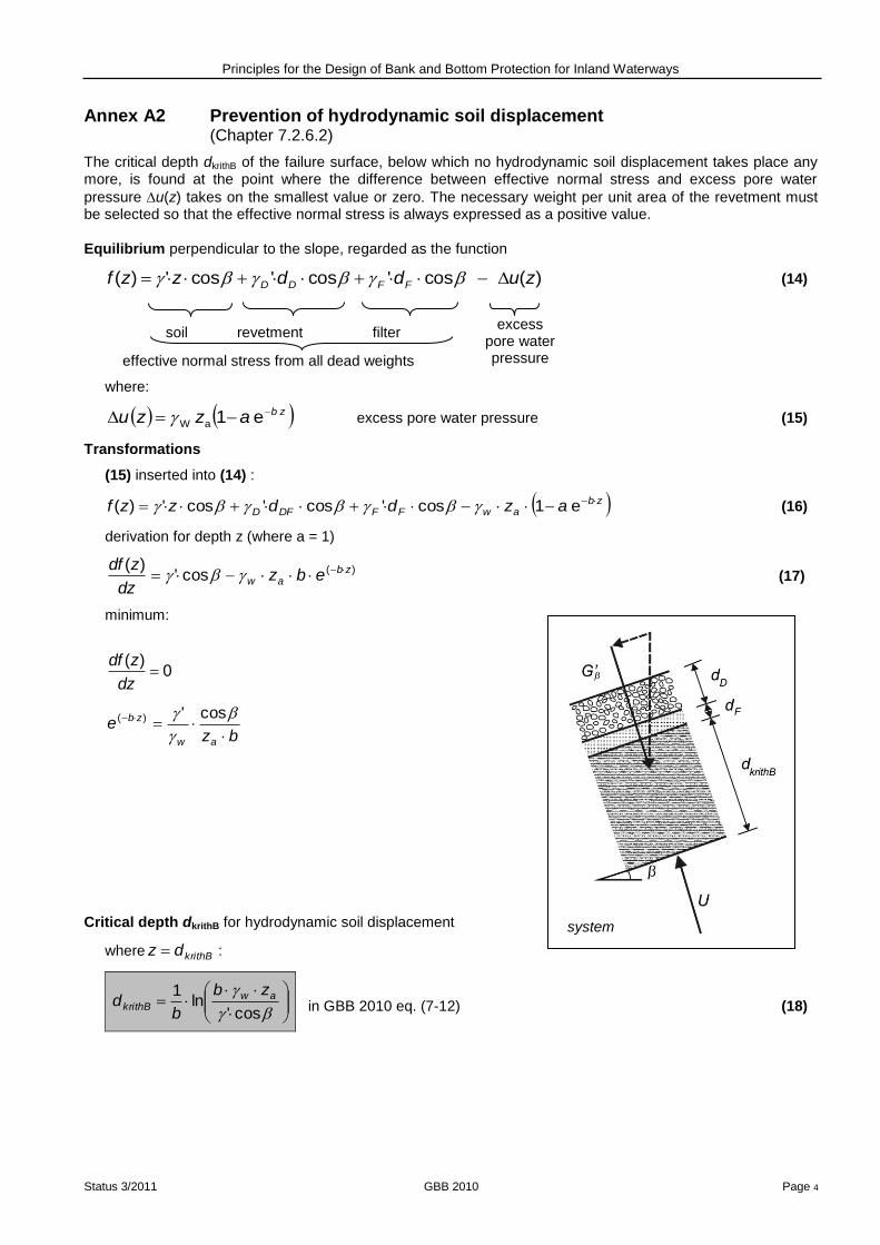
Principles for the Design of Bank and Bottom Protection for Inland Waterways
Status 3/2011 GBB 2010 Page 4
Annex A2 Prevention of hydrodynamic soil displacement (Chapter 7.2.6.2)
The critical depth dkrithB of the failure surface, below which no hydrodynamic soil displacement takes place any more, is found at the point where the difference between effective normal stress and excess pore water
pressure u(z) takes on the smallest value or zero. The necessary weight per unit area of the revetment must be selected so that the effective normal stress is always expressed as a positive value.
Equilibrium perpendicular to the slope, regarded as the function
)(cos'cos'cos')( zuddzzf FFDD (14)
where:
zbazzu e1aW excess pore water pressure (15)
Transformations
(15) inserted into (14) :
zbawFFDFD azddzzf e1cos'cos'cos')( (16)
derivation for depth z (where a = 1)
)(cos')( zb
aw ebzdz
zdf
minimum:
0)(
dz
zdf
bze
aw
zb
cos')(
Critical depth dkrithB for hydrodynamic soil displacement
where krithBdz :
cos'ln
1 awkrithB
zb
bd in GBB 2010 eq. (7-12) (18)
soil revetment filter excess
pore water pressure effective normal stress from all dead weights
(17)
system

Principles for the Design of Bank and Bottom Protection for Inland Waterways
Status 3/2011 GBB 2010 Page 5
Equilibrium perpendicular to the slope:
U cos G' G' (19)
)1(cos'cos'cos')( krithBdb
awkrithBFFDD ezddd
(20)
cos)''()1(cos')(
krithBFFdb
awDD ddezd krithB (21)
Required surcharge (= superimposed load) g’ for the prevention of hydrodynamic soil displacement:
)''(cos
'' krithBFFDD ddu
dg
in GBB 2010 eq. (7-11) (22)
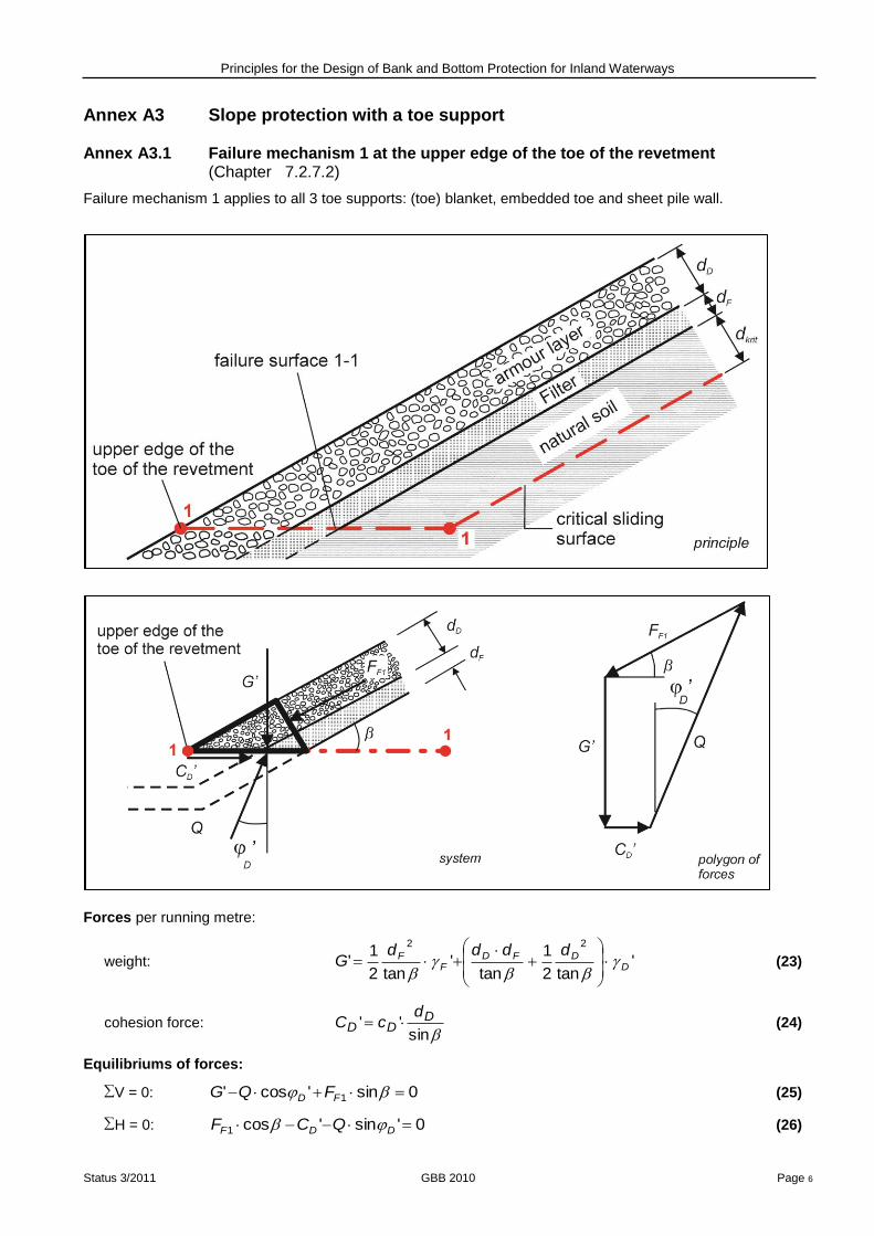
Principles for the Design of Bank and Bottom Protection for Inland Waterways
Status 3/2011 GBB 2010 Page 6
Annex A3 Slope protection with a toe support
Annex A3.1 Failure mechanism 1 at the upper edge of the toe of the revetment (Chapter 7.2.7.2)
Failure mechanism 1 applies to all 3 toe supports: (toe) blanket, embedded toe and sheet pile wall.
Forces per running metre:
weight: 'tan2
1
tan'
tan2
1'
22
DDFD
FF dddd
G
(23)
cohesion force: sin
'' DDD
dcC (24)
Equilibriums of forces:
V = 0: 0sin'cos' 1 FD FQG (25)
H = 0: 0'sin'cos1 DDF QCF (26)
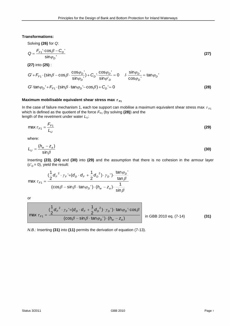
Principles for the Design of Bank and Bottom Protection for Inland Waterways
Status 3/2011 GBB 2010 Page 7
Transformations:
Solving (26) for Q:
'sin
'cos'1
D
DF CFQ
(27)
(27) into (25) :
'tan'cos
'sin/0
'sin
'cos')
'sin
'coscos(sin' 1 D
D
D
D
DD
D
DF CFG
0')cos'tan(sin'tan' 1 DDFD CFG (28)
Maximum mobilisable equivalent shear stress max F1
In the case of failure mechanism 1, each toe support can mobilise a maximum equivalent shear stress max F1
which is defined as the quotient of the force FF1 (by solving (28)) and the length of the revetment under water LU:
U
FF
L
F 11max (29)
where:
sin
)( awU
zhL
(30)
Inserting (23), (24) and (30) into (29) and the assumption that there is no cohesion in the armour layer
(c’D = 0), yield the result:
sin
1)()'tansin(cos
tan
'tan)')
2
1('
2
1(
max
22
1
awD
DDDFDFF
F
zh
dddd
or
)()'tansin(cos
cos'tan)')2
1('
2
1(
max
22
1
awD
DDDFDFF
Fzh
dddd
in GBB 2010 eq. (7-14) (31)
N.B.: Inserting (31) into (11) permits the derivation of equation (7-13).

Principles for the Design of Bank and Bottom Protection for Inland Waterways
Status 3/2011 GBB 2010 Page 8
Annex A3.2 Failure mechanism 2 with a toe support
The verification in failure mechanism 2 differs according to the type of support.
Annex A3.2.1 Failure mechanism 2 with a toe blanket (Chapter 7.2.7.3)
In the case of a toe blanket, verifications for failure mechanism 2 must be carried out inside and outside the toe blanket (failure surfaces 2i and 2a respectively).
A) Verification inside
System sketch for determining the toe support force max FF2,i within the toe blanket:
Equilibriums of forces
∑V = 0: 0sinmax''cos 2 FDFDFDF FGQ (32)
∑H = 0: 0cosmax'sin 2 FDFDF FQ (33)

Principles for the Design of Bank and Bottom Protection for Inland Waterways
Status 3/2011 GBB 2010 Page 9
Transformations
Solving (33) for Q:
DFDF
FFQ
'sin
cosmax 2
Inserted into (32) and where
2
'45 DF
DF
is the angle of the sliding surface (34)
results in max FF2 :
sin'cotcos
'max 2
DFFD
F
GF (35)
where
DF
DFFFDF
DF
FFFF
DF
DFDF ddddG
tan
'
tan2
'
tan2
''
22
is the effective weight (36)
Maximum mobilisable equivalent shear stress max F2,i
In failure mechanism 2 (verification inside) a maximum equivalent shear stress of max F2,i is mobilised, which
is defined analogously to (29):
u
FiF
L
F 2,2
maxmax
(37) With (35) and (36) and also (30) the following is obtained:
)z(h
dddd
awDFDFDF
DFFFDFFF2
FFDF
2
DF
iF2,tan2sincotcos
sin2
max
in GBB 2010 eq. (7-16) (38)
corresp. to
G’D1
corresp. to G’F
corresp. to
G’D2

Principles for the Design of Bank and Bottom Protection for Inland Waterways
Status 3/2011 GBB 2010 Page 10
B) Verification outside
System sketch for determining the toe support force max FF2,a outside the toe blanket:
Equilibriums of forces
∑V = 0: 0sinmax´'cos 2 aFGQ (39)
∑H = 0: 0''sincosmax 2 pha EQF (40)
Transformations
Solving (39) for Q and inserting into (40):
´tansincos
'´tan´max 2
ph
a
EGF (41)
Maximum mobilisable equivalent shear stress max F2,a
In failure mechanism 2 (verification outside), a maximal equivalent shear stress
max F2,a will be mobilised, which is defined analogously to (29):
u
aaF
L
F2,2
maxmax
results in:
aw
phFuv
aF2,'tansincos
sin'''tan'max
zh
ELc
in GBB 2010 eq. (7-17) (42)
system

Principles for the Design of Bank and Bottom Protection for Inland Waterways
Status 3/2011 GBB 2010 Page 11
Passive earth pressure E’ph
For the maximum equivalent shear stress max F2,a according to (42), the passive earth pressure acting in front
of the toe blanket E’ph may be allowed for.
System sketch for determining the passive earth pressure E’ph :
Equilibriums of forces
(1) ∑V = 0: 0''cossin GUQC VPP (43)
(2) ∑H = 0: 0''sincos phPP EQC (44)
Passive earth pressure Eph’ in front of the toe blanket
Solving (43) for Q’ and insertion into (44) and solving for Eph’ gives the result:
pppvph CCUGE cos'tansin'' in GBB 2010 eq. (7-21) (45)
with the following auxiliary functions:
2
'45
P
p
kritF ttG
tan2
'2
p
kritF ttcC
sin
'
kritFtb
tbtb
p
awv tte
b
eezU krit
kritF
tan
system

Principles for the Design of Bank and Bottom Protection for Inland Waterways
Status 3/2011 GBB 2010 Page 12
Annex A3.2.2 Failure mechanism 2 with an embedded toe (Chapter 7.2.7.4)
In the case of an embedded toe, for failure mechanism 2, a left-hand soil wedge in front of the toe embedment
(sliding surface angle P ) and a right-hand soil wedge with the embedded revetment (slope angle ) must be
considered when determining the achievable equivalent shear stress of the toe support.
Sketch of the entire system of the toe embedment
Geometric parameters
sin
kritkawu
ttzhL
(46)
´tan
tan´tan
´tan´tan1arctan
2
P angle of sliding surface (47)
awkrit
zb
bt ln
1 critical depth = fluidisation depth from (18) where = 0 (48)
Left-hand soil wedge (1)
- In the left-hand soil wedge, no soil weight is assumed in the area of the critical depth tkrit. - In the remaining area of soil, a vertical excess pore water pressure Uv1 is allowed for. - For the transfer of forces between the left- and right-hand soil wedges, an internal force Fint is introduced.
System sketch of the left-hand soil wedge for determining the internal force Fint
system
Underwater length of the revetment, allowing for scour depth (guideline) and critical depth [according to (48)]

Principles for the Design of Bank and Bottom Protection for Inland Waterways
Status 3/2011 GBB 2010 Page 13
Vertical excess pore water pressure Uv1
System sketch of the left-hand soil wedge for determining the excess pore water pressure Uv1
Distribution of the excess pore water pressure in the remaining, unfluidised soil:
kritkritkritF
kritF
krit
btbtFF
btbtF
P
aw
kritFbt
P
awt
t
bt
P
awv
btaw
P
P
kritFkritv
ettetteb
teb
tz
ttez
dtez
U
eztudt
dx
tttudxxuU
000
1
1
11
tan
1tan
1tan
1andtan
w ith
tan
kritFbt
btbt
P
awv tte
b
eezU krit
kritF
tan1 (49)
Equilibriums of forces
∑V = 0: 0sin´cossin int1111 FGUQC vPP (50)
∑H = 0: 0cos´sincos int11 FQC PP (51)
Transformations
Solving (51) for Q1:
P
PCFQ
´tan
coscos 1int1 (52)
(52) into (50):
0sin
´tan
coscossin int11
1int1
FGU
CFC v
P
PP
system

Principles for the Design of Bank and Bottom Protection for Inland Waterways
Status 3/2011 GBB 2010 Page 14
Internal force Fint
Solving for Fint:
P
PvP
P
CUGCF
´tan
cossinsin
´tan
cos1111int
P
P
PPv CGU
F
´tan
cossin
´tan
cossin111
int (53)
where
P
kritF ttG
tan2
1 2
1
P
kritF ttcC
sin1
Right-hand soil wedge (2)
- In the right-hand soil wedge, no soil weight is assumed in the area of the critical depth tkrit. - In the remaining area of soil, a vertical excess pore water pressure Uv2 will be allowed for. - For the transfer of forces between the left- and right-hand soil wedges, an internal force Fint according to (53) is used.
System sketch of the right-hand soil wedge for determining the internal force Fint
Vertical excess pore water pressure UV2
Analogously to (49), the following is true for P :
kritFbt
btbtaw
v tteb
ee
tan
zU krit
kritF
2 (54)
system

Principles for the Design of Bank and Bottom Protection for Inland Waterways
Status 3/2011 GBB 2010 Page 15
Equilibriums of forces
∑V = 0: 0sinsinsin´cos 2int2222 Fv FFCQUG (55)
∑H = 0: 0coscos´sincos 222int FFCQF (56)
Transformations
Solving (56) for Q2:
sin
cos2int22
CFFQ F (57)
(57) into (55) and order:
0sinsinsin´cotcos 2int22int222 FFv FFCCFFUG
´cotcossin
´coscos
´cotcossinsinsin´cotcos
int222
22
int222
FCGU
CG
FCUF
v
vF
Achievable shear force FF2
Solving for FF2:
int222
2´cotcossin
FCGU
F vF
(58)
where
tan2
1 2
2
kritF tt
G
sin
2kritF ttc
C
(58) with (53):
2
221112
´cotcossin´cotcossin
´cotcossinC
GUCGUF v
P
PPPvF
222111
2 CD
GU
B
ACGUF vv
F
in GBB 2010 eq. (7-24) (59)
where
´cotcossin
´cotcossin
´cotcossin
D
B
A
P
PPP

Principles for the Design of Bank and Bottom Protection for Inland Waterways
Status 3/2011 GBB 2010 Page 16
Annex A3.2.3 Failure mechanism 2 for a toe sheet pile wall (Chapter 7.2.7.5)
In the case of the sheet pile wall at the toe, determining the earth pressure ordinate e'ph is important for failure mechanism 2.
System sketch for determining eph
Geometric parameters
´tan
tan´tan
´tan´tan1arctan
p
2
p angle of the sliding surface (60)
bz
bt awkrit ln
1 critical depth = fluidisation depth from (18) where = 0 (61)
Excess pore water pressure Uv
Analogous to (49):
kritFbt
btbt
P
awv tte
b
eezU krit
kritF
tan (62)
Equilibriums of forces
∑V = 0: 0sinsin´cos pPPPv ECQUG (63)
∑H = 0: 0cos´sincos pPPP EQC (64)
Transformations
Solving (64) for Q:
´sin
coscos
P
PpP CEQ (65)
(65) into (63) and order:
0sin'sin´cotcoscos' pPPPPppv ECCEUG
´cotcossin´cotcossin PPPvPppP CCGUE
system

Principles for the Design of Bank and Bottom Protection for Inland Waterways
Status 3/2011 GBB 2010 Page 17
Horizontal earth pressure ordinate e’ph
Solving for earth resistance E’p
´cotcossin
sin´cotcos
Ppp
PPPvp
CGUE (66)
where
P
kritF ttcC
sin
P
kritF ttG
tan2
2
horizontal component
of the passive earth resistance
(see system sketch on right)
FphkritFPpph tettEE 2
1cos
kritF
PFph
tt
Ete
cos2 in GBB 2010 eq. (7-28) (67)
system
sheet pile wall

Principles for the Design of Bank and Bottom Protection for Inland Waterways
Status 3/2011 GBB 2010 Page 18
Annex A3.2.4 Required weight per unit area of the armour layer above the lowered water level in the case of a revetment suspension
(Chapter 7.2.8.2)
For a revetment suspension, the tensile force Z that must be withstood is obtained by multiplying the required
shear stress erf according to eq. (7-10) depending on the selected thickness of the revetment dD, by the length Lu of the armour layer that lies below the lowered water level.
Forces per running metre
uAerf LZ (68)
oABAB LcC ' (69)
where Lo is the length of the revetment suspension above the lowered water level (must be specified)
oFoFoDoDoDo LddG (70)
Equilibriums of forces
∑V = 0: 0'cossin'sin ABABDo QCZG (71)
∑H = 0: 0'sincos'cos ABAB QCZ (72)
Transformations
Solving (72) for Q:
AB
ABCZQ
'sin
cos'cos (73)
(73) into (71) and solving for GDo:
0'sin
'coscos'cossin'sin
AB
ABABABDo
CZCZG
system

Principles for the Design of Bank and Bottom Protection for Inland Waterways
Status 3/2011 GBB 2010 Page 19
AB
ABABABABABDo
CZG
'sin
'sinsin'coscos''sinsin'coscos
with the angle function
ABABAB 'cos'sinsin'coscos
AB
ABABABDo
CZG
'sin
'cos''cos (74)
Required weight per unit area g’
(69) and (70) into (74)
FoFo
ABo
ABoABABDoDo d
L
LcZdg
'sin
'cos''cos' in GBB 2010 eq. (7-29) (75)

Principles for the Design of Bank and Bottom Protection for Inland Waterways
Status 3/2011 GBB 2010 Page 20
Annex B Flow chart for carrying out the geotechnical design
dD,BM1
without toe support
revetment suspension
embedded toe
Fracture mechanism 1
toe blanket toe sheet pile wall
Fracture mechanism 2
Geotechnical design of an armour layer
(Verification of the local stability for determining the required armour layer thickness erf dD,geo)
permeable armour layer
(loose or partly grouted)
unbound armour layer
partially grouted armour layer
erf dD,geo = dD,hB erf dD,geo = dD, abheben
dD, equation 7-2
where F = A = 0
erf dD,geo = Max
{dD,abgleiten, dD,hB}
erf dD,geo = Max {dD,hB, dD,BM1, dD,BM2}
erf dD,geo = Max ( dD,hB, dD,BM1)
dD,BM1
without toe support
with toe support
Failure mechanism 1
Failure mechanism 2
Geotechnical design of an armour layer
(Verification of the local stability for determining the required armour layer thickness erf dD,geo)
verifiation of resistance to hydrodynamic soil
displacement dD,hB
verification of resistance to uplift
dD,abheben
verification of resistance to sliding
failure dD,abgleiten
impermeable armour layer
(full grouting or impervious lining)
ungrouted armour layer
partially grouted armour layer
erf dD,geo = Max {dD,abgleiten, dD,abheben}
erf dD,geo = dD,hB
without toe support with toe support
verification of resistance to
uplift dD,abheben
erf dD,geo = dD,abheben
erf dD,geo = dD,hB
dD,BM2 = f(tf,Plan, LFu) dD,BM2 = f(tf,Plan) calculation of input values for sheet pile wall
statics
dD acc. to
eq. (7-9)
where
F = A = 0
calculation of tensile force for the design of the
suspension
erf dD,geo = Max {dD,hB, dD,BM1}
Note: When determining the required thickness of an armour layer erf dD the minimum
thicknesses min dD should be considered subsequently in addition to erf dD,geo.
verification of resistance to sliding failure dD,abgleiten
Only with
excess pressure
from groundw
ater
!!

Principles for the Design of Bank and Bottom Protection for Inland Waterways
Status 3/2011 GBB 2010 Page 21
Annex C Determination of an equivalent trapezoidal profile
With reference to Chapter 5.2.1 “Geometry of waterways”
The hydraulic calculation methods in Chapter 5 are based on a trapezoidal waterway cross section with a constant water depth. These methods may be also used as approximations for an irregular cross section, if this can be approximated using an equivalent trapezoidal cross section. If the bank which is to be designed is situated on the left-hand side of the irregular cross section, this must first be mirror-imaged around the axis of the cross section, as the right bank is always used for the design procedure. Subsequently, the equivalent trapezoidal cross section can be constructed according to the following principles, which are listed in order of their importance. The general restriction to largely prismatic cross sections, which thus may only be altered slightly in the direction of motion, is still applicable here, so that the general assumption of the quasi-steady motion assumed in Chapter 5 continues to be relevant.
1. The mean water depth hSP in the area of the ship’s path largely determines the possible ship
speed and, thus, the water level drawdown. For this reason hSP should be selected as the water
depth h of the equivalent trapezoidal cross section.
2. The slope inclination of the right bank as the design bank mrts,real in the real cross section,
especially as averaged in the zone of fluctuating water levels, is decisive for the stability of the revetment. It should match the right-hand slope inclination in the equivalent trapezoidal profile.
3. The largest distance between the ship and the design bank ureal in the real cross section should
match the distance u in the equivalent trapezoidal profile so that the formulae for the decline in the drawdown between the ship and the bank and of the shoaling of the waves near the bank can be depicted correctly.
The distance of the ship from the opposite bank of the real profile should also be reflected in the equivalent trapezoidal profile, so that the decline function, which also depends in large ship to bank distances on the position of the ship in the cross section, as shown in Annex C, can be stated correctly. Only if the distance to the left bank is many times larger than half the influence width of the return flow field, can the cross section be cut off there; see sketch below.
4. Besides the water depth, the achievable ship speed and the water level drawdown are determined by the cross-sectional area occupied by the return flow field and, consequently, the related n-ratio. This part of the cross-sectional area in the real profile Areal should therefore correspond to the area A of the equivalent trapezoidal cross section (parity of cross section).
A diagrammatic example for the application of these principles is shown below. The area without impact on the return flow according to distance case C in Chapter 5.5.1.1 is cut off towards the left bank. If the real cross section shape is too strongly deformed by this, the area with impact on the return flow should be enlarged. In the example it is possible to apply all four of the above-mentioned principles, and after selection of h, mrts and mlks, the as yet unknown water surface width bWS in the
equivalent trapezoidal profile can be recalculated from the requirement of identical cross-sectional areas in the critical cross-section area of the real profile. In the example, the width of the equivalent trapezoidal cross section thus becomes somewhat larger than the reading from the real cross section. This is because the water depths in the left-hand cross-sectional area are on average larger than hSP.

Principles for the Design of Bank and Bottom Protection for Inland Waterways
Status 3/2011 GBB 2010 Page 22

Principles for the Design of Bank and Bottom Protection for Inland Waterways
Status 3/2011 GBB 2010 Page 23
Annex D: Change in the mean return flow velocity between ship and bank for slender ships and small drawdown
With reference to Chapter 5.5 “Magnitude of ship-induced waves (design situation: ‘sailing at normal speed’)”
Below we will show the derivation of approximation formulae for the modification of return flow velocity and drawdown between the ship and the bank. We will assume vessels that are “slender” in proportion to their length and to the width of the canal. This means, for example, that the proportion of the return flow field beneath the ship can be disregarded. Furthermore, by simultaneously assuming that the drawdown is small in proportion to the water depth h, the flow field around the ship can be understood as a plane problem, corresponding to a constant flow velocity over the water depth, which is similarly assumed to be constant. In the case of a small drawdown, the distribution of the latter across the width of the waterway is identical to that from the return flow field. Finally, in a further simplification, the inland navigation vessel will be considered as having an elliptical shape, which along with the assumption of a frictionless flow, permits a largely analytical description of the flow field around the ship.
These simplifications mean that the relative change (i.e. in relation to the value at the ship) of the return flow velocity, and therefore also of the drawdown towards the bank (decline function), can be made to depend on only a small number of influencing parameters, such as the calculated waterway width br, the related distance of the ship from the design bank ur,rts, the effective ship length Leff and the beam of the ship B. The same is true for the influence width of the return flow field bE and the
associated calculated width of the equivalent R-profile br,äqui, which reflects the progress of the decline function. Of course, the decline function is also influenced by the contours of the ship, particularly in the case of compact ship hulls and small ratios of draught T to water depth h (in both instances a smaller influence width will result than according to the present theory), but this influence is of less significance than that of the above-mentioned parameters and can therefore be disregarded.
Next, the case of a ship in an infinitesimally large fairway will be considered in order to derive the base equations for the distribution of velocities, to derive a useable formula for the influence width bE
and to demonstrate the linear dependence of the drawdown h on the return flow velocity vrück. Subsequently, a fairway that is confined on one side (towards the right bank) will be considered in order to explain the mirror image principle that will finally also be used for fairways that are confined in all dimensions, from which the general relationship of the decline function is derived.
1) A ship in a fairway of infinite width
Approximation of a ship using a source-sink flow
The plane potential flow between a source (logarithmic potential 1, source strength Q) and a sink (potential 2), that is, a dipole flow (distance between the poles = a) in combination with the approach flow of the ship (speed vS from the perspective of an observer moving with the ship, potential 3), forms a flow line in the shape of an ellipse, which should approximate the contours of the ship; see sketch below. This flow line separates the area of the inner flow between the poles (in the ship) from the outer flow, that is, the flow field around the ship which is of interest here. According to the laws of
potential flow, the potentials are superposed linearly to the overall potential as shown below. From this, the flow velocities are obtained by the formation of gradients.

Principles for the Design of Bank and Bottom Protection for Inland Waterways
Status 3/2011 GBB 2010 Page 24
Source (1):
2221
211 yxr,rln
4
Q
Sink (2):
2222
222 yxar,rln
4
Q
Natural flow (3):
xvS 3
Superposition:
321
By differentiating the function with respect to x the speed component in vS – direction vx is obtained.
In order to obtain the related return flow velocity vrück (also known as “disturbance flow velocity” or “overspeed”), which would be registered by a stationary observer, the ship speed must per definition be deducted. It will subsequently be determined from the source and sink term.
2
2
2
1
Sxr
xa2
r
x2
4
Qv
xv
For vx at the centre of the ship (where x = a/2) the following result is obtained:
v vˆ
y2
a
2
a
Qv
2
axv rückS
2
2Sx
Integrating this vx distribution over y results in an equation for the associated discharge. In the area of
the assumed flow line, which separates the inner from the outer flow, this must correspond to the source strength Q, since the source-sink flow produces the outer flow of the ship through displacement. If the requirement is that this should be the case over the beam of the ship B, then a conditional equation is obtained for Q:
Proportion of disturbance flow vrück
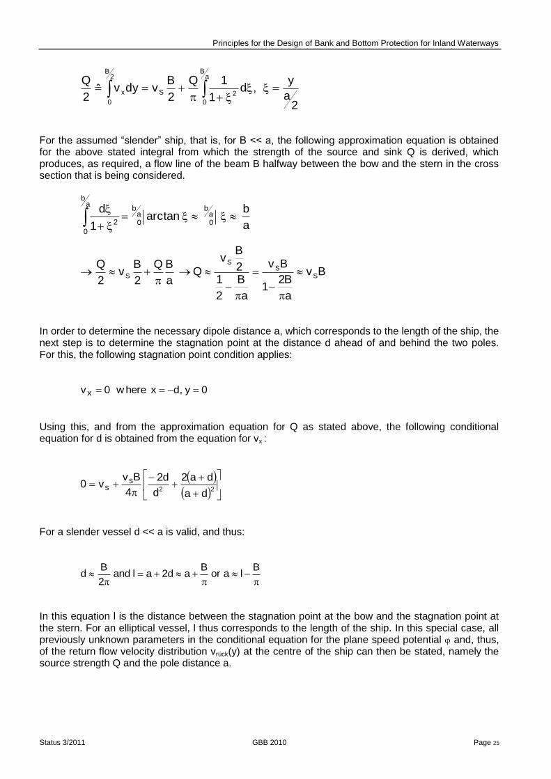
Principles for the Design of Bank and Bottom Protection for Inland Waterways
Status 3/2011 GBB 2010 Page 25
2a
y,d
1
1Q
2
Bvdyvˆ
2
Q aB
0
2S
2B
0
x
For the assumed “slender” ship, that is, for B << a, the following approximation equation is obtained for the above stated integral from which the strength of the source and sink Q is derived, which produces, as required, a flow line of the beam B halfway between the bow and the stern in the cross section that is being considered.
a
b
0
ab
0a
b
02 a
barctan
1
d
Bv
a
B21
Bv
a
B
2
12
Bv
Qa
BQ
2
Bv
2
QS
SS
S
In order to determine the necessary dipole distance a, which corresponds to the length of the ship, the next step is to determine the stagnation point at the distance d ahead of and behind the two poles. For this, the following stagnation point condition applies:
0y,dxw here0vx
Using this, and from the approximation equation for Q as stated above, the following conditional equation for d is obtained from the equation for vx :
22
SS
da
da2
d
d2
4
Bvv0
For a slender vessel d << a is valid, and thus:
Blaor
Bad2aland
2
Bd
In this equation l is the distance between the stagnation point at the bow and the stagnation point at the stern. For an elliptical vessel, l thus corresponds to the length of the ship. In this special case, all previously unknown parameters in the conditional equation for the plane speed potential and, thus, of the return flow velocity distribution vrück(y) at the centre of the ship can then be stated, namely the source strength Q and the pole distance a.

Principles for the Design of Bank and Bottom Protection for Inland Waterways
Status 3/2011 GBB 2010 Page 26
Influence width of the return flow field:
With the above stated equations, it is possible to obtain, amongst others, the return flow velocity at
the ship vrück(y = B/2) = vRmax. Under canal conditions (width case “A” in Chapter 5.1.1.1) this value is
constant across the canal width and can be calculated according to the one-dimensional canal theory
as in Chapter 5.5.3. The latter can also be applied in the general case under consideration here of a
plane flow around the ship, if the entire discharge which constitutes the return flow field beside the
ship is imagined as being included in a width bm that has still to be determined, and the return flow
velocity there assumes the maximum constant value vRmax. If this is again used as a simplification for
the centre of the ship (x = a/2), and if the ship beam B is allowed for, where there is no impact from
the return flow in the external field, then the width bm is obtained as demonstrated in the following
illustration, which shows the return flow distribution in diagram form, from the condition that the entire
return flow is led away over the cross-sectional area hBbm with maxRv .
dyvv2Bbv
2B
v
Sx
!
mmaxR
rück
Using this conditional equation for vRmax, the integration over the entire area affected by the return flow can then be carried out and assessed quantitatively for a slender vessel and, from this the width bm, over which the return flow field can be consolidated, can be obtained. This width is described in Chapter 5.5.1.1 as the influence width of the return flow field bE.
aBfora
Q2
a
B1
1
a
Q2
2
B
2
a
2
a
Q
2
By,
2
axvv
222rückmaxR
dady,a
y,dy
y2
a
2
a
Q2Bb
a
Q2
2
B 2
2m

Principles for the Design of Bank and Bottom Protection for Inland Waterways
Status 3/2011 GBB 2010 Page 27
1a
Bfor
a
B2
a2
B
a2
B 2
2ma
Barctanarctan
Q22arctan2
Qd
2
1
1QBb
a
Q2
a
B
2
Q2Bb
a
Q2m
Emm ba2
ba
B
2aBb
Approximation of a real inland navigation vessel using an ellipse:
As a real inland navigation vessel is not elliptical, a or l must be linked with the usual ship dimensions L and B with regard to bE. To do so, it can be assumed that the flow ahead of the vessel (in sketch
below, left-hand side) splits at an angle of 1:1 and is reunited behind the ship at a separation angle of 1:5. For a rectangular, slender vessel the following relationships ensue between the length of the ellipse and the dimensions of the ship:
3f,BfLl B
From this, with the relationship between l and a that is derived from the stagnation point condition, the sought for equation for bm or bE is obtained:
1fBL
2
Bl
2a
2b Bm
Since 1/ fB for an inland navigation vessel with a rectangular contour, the values for the sought after relationships between the ship dimensions and bm and also a can be found. As a result, the decline function can now be quantitatively evaluated.

Principles for the Design of Bank and Bottom Protection for Inland Waterways
Status 3/2011 GBB 2010 Page 28
B3L2
bm
and
B3La
This will be explained using the example of a large inland cargo vessel with a length of 105 m and a beam of 11 m: From the equations for vrück and vRmax using the previously stated relationships, a
relationship for the ratio between vrück and vRmax, can be obtained, which depends only on the relative
distance = y / a, that is, with reference to the dipole distance a. This relationship is applied for the GMS (large inland cargo vessel) and is illustrated below.
a
y,
2
1
4
1
y2
a
2
a
Q
Q2
a
v
v:
2
by
0.1v
v:
2
by
)hˆt,problemplane(0v:2/By0
1
22
22
maxR
rücks
maxR
RS
SR
Accordingly, the bell-shaped curve of the decline function for the large inland cargo vessel in a laterally unrestricted fairway can be roughly approximated using the following reference values, in order to estimate the extent to which the return flow velocity declines towards the design bank.
Lyat3
1
L3/2y.approxat2
1
L3/1y.approxat5
4
v
v
maxR
rück

Principles for the Design of Bank and Bottom Protection for Inland Waterways
Status 3/2011 GBB 2010 Page 29
Linear relationship between drawdown and return flow velocity
In order to be able to utilise the above mentioned relationships for the distribution of the return flow velocity beside the vessel for the related drawdown h, Bernoulli's equation for potential flows will be
used for the assumed condition h << h, where a point far ahead of the ship (flow velocity = vS) is
compared with a second point in the cross section at the centre of the ship, in which vx is identical to
the amount of the resulting speed vector:
rückSx
2
x
2
S vvv;hhg2
vh
g2
v
1
v
v1
g2
v1
v
v
g2
vvv
g2
1h
2
S
rück
2
S
2
S
x
2
S2
S
2
x
According to this, for assumed return flow velocities that are small in comparison to the velocity of the
ship, h is directly proportional to vrück, providing an equation for the ratio of the drawdown at the
distance y from the axis of the ship h to the drawdown at the ship maxh . Because of this equation
the progression of the decline function in Figure 5.7 in Chapter 5.5.1.1 under the above stated
conditions for vrück,u,rts and h u,rts is identical.
g
vv
v
v2
g2
vh rückS
S
rück
2
S
maxR
rück
maxv
v
h
h
2) A ship in a fairway confined at one side
Because of the superposition principle of potential flows, motion in a laterally confined fairway can be described as shown in the sketch below and the following equations by superposition of the flow fields of two ships which are underway in sailing lines that are symmetrical with regard to the bank. The superposition yields a flow line at the right bank, which is assumed to be perpendicular. In the case of inclined slopes the relevant bank distance ur,rts is to be taken as the value of the equivalent R-profile according to Figure 5.5.

Principles for the Design of Bank and Bottom Protection for Inland Waterways
Status 3/2011 GBB 2010 Page 30
xvvandxv xB2B1A2A1
N.B.: ur,rts and ur,lks describe the distance of the ship from the bank and must therefore both be positive
values.
For slender ships, that is, for B << a, it can be assumed as an approximation that the boundary conditions which apply to the ship in fairways confined at both sides will also be true for the superposition, i.e., the closed flow line which the ship forms is still at the distance y = B/2 and the stagnation point is at x = d. For x = a/2 the following equations apply as an approximation for the discharge between the two dipoles A and B, which form the flow field, for the related superposed return flow velocities and, finally, for the relationship between the velocities at the distance y from the ship and the value at the ship:
QˆBv
a
B21
BvQQ S
SBA
2rts,r
2
2
2rück
u2y2
a
2
a
Q
y2
a
2
a
Qv
2
rts,r
2
2
2rück
u2y2
a
1
y2
a
1
2
Qav
xxyy AA
!!
,
rts,rAB u2yy
rts,rB u2yy
xxx AB

Principles for the Design of Bank and Bottom Protection for Inland Waterways
Status 3/2011 GBB 2010 Page 31
2
rts,r
222maxR
u22
B
2
a
1
2
B
2
a
1
2
Qav
12
rts,r
21
22
1
2
rts,r
21
2
2
maxR
rts
u22
B
2
a
2
B
2
a
u2y2
ay
2
a
v
v
With the introduction of the following definitions the equation for the decline functionvrück / vRmax can
be written in dimensionless form. The dipole distance a was selected as the scaling length.
a
y , au r
!
rts,r , aB!
It follows, therefore, that the decline function, beside the relative distance, i.e. the distance y relative to a, depends on only two further parameters: the relative bank distance r and the relative beam of the ship (the slenderness of the ship).
max
12
r
21
22
1
2
r
21
2
2
maxR
rück
h
h
222
1
22
1
22
1
2
1
v
v
Applied to a large inland cargo vessel with a length of 105 m and a beam of 11 m (a = 138 m, = 0.10) and e.g. for a bank that lies at a distance equivalent to the ship length ( = r = 0.76), this equation produces a value of 0.57 for the decline function. In an infinitesimally wide fairway this value according to the above statements would be 0.30. When a ship is underway close to the bank, the return flow field thus declines much more weakly than when there is no influence from the bank.
3) A ship underway in a fairway that is confined in all dimensions (canal)
The mirror image principle can also be used for fairways laterally confined at both sides. In order to produce the desired flow lines at both banks, the mirror imaging at the right bank with dipole B, which has already been described, must first be repeated for the left bank, as in the sketch below. This is carried out using the dipole D, which, however, also produces a disturbance potential at the right bank, which deflects the flow line there towards the right as a result of the displacement effect of the ship D. In order to compensate for this effect, a dipole C can be added, which compensates for the displacement effect of dipole D, but which now again deflects the flow line of the left bank, so that a further dipole should be positioned at position E. This observation shows that the flow lines at the left and right banks can only be produced with an infinite continuation of the mirror image principle.

Principles for the Design of Bank and Bottom Protection for Inland Waterways
Status 3/2011 GBB 2010 Page 32
Nevertheless, the superposition of 5 dipoles as shown in the sketch below and the relevant geometrical boundary conditions should first be studied, from which analogously to the simple superposition, the following equation for the decline function is obtained:
2
axxxxx EDCBA
rtsrlksrAElksrADlksrrtsrACrtsrrtsrABA uuyyuyyuuyyuyuyyyy ,,,,,,, 2,2,2,22,
a
u
a
u
a
B
a
y lksr
l
rtsr
r
,,,,,
12
rl
221
2
l
221
2
rl
21
2
r
21
22
1
2
rl
21
2
l
21
2
rl
21
2
r
21
2
2
maxR
R
2222
12
22
122
22
12
22
1
22
1
222
12
2
122
2
12
2
1
2
1
v
v
In the standard R-profile (width 42 m) according to the Guidelines for Standard Cross Sections, a value of 0.99 for the decline function is obtained using this equation for the large inland cargo vessel underway in the middle of the waterway, which has already been discussed several times. This demonstrates that the return flow velocity in the canal situation is indeed more or less constant.
For a further mirror image, the following term is also included in the numerator in the above mentioned equation:
1
2
rl
21
2
lr
2
242124
21
Accordingly the denominator is:
12
rl
21
2
lr
2
2422
12422
1

Principles for the Design of Bank and Bottom Protection for Inland Waterways
Status 3/2011 GBB 2010 Page 33
A further mirror imaging procedure must be supplemented with the following:
numerator: 1
2
rl
21
2
rl
2
442144
21
denominator:
12
rl
21
2
rl
2
4422
14422
1
This demonstrates the law of formulation for n mirror imaging steps. With the following definitions a generally valid equation for the decline function can finally be obtained with which the diagrams according to Figure 5.7 were calculated.
It is precisely valid for n . For the numerical evaluation usually only a few mirror images are sufficient. Therefore one possibility is to use the formula for successively increased values of n until there is no further significant change in the desired function value.
a
u,
a
u,
2a2
B,
a
yw ith,
v
v rts,rr
lks,rl0
0maxR
rück
n
1i
1
2rl
21
2rl
2
n
1i
1
2rl
21
2rl
21
22
n2n22
11n2n2
2
1
n2n22
1n21n2
2
1
2
1
4) Width of the equivalent canal cross section
Analogously to the definition of the influence width of the return flow field, a canal width of br,äqui can
also be defined in the general case of a fairway confined in all dimensions, in which one can imagine
the entire return flow field being concentrated when it takes on the maximum value at the ship at this
width. This leads to the equation below, in which, if slender vessels are assumed, the return flow field
beneath the ship can again be disregarded.
dyyvdyyvBbv
2B
rück
2B
rückäqui,rmaxR
With the definitions a
Band
a
y this results in:
dda
b
20
2
0
äqui,r

Principles for the Design of Bank and Bottom Protection for Inland Waterways
Status 3/2011 GBB 2010 Page 34
In GBBSoft the two above stated integrals in the equation for br,äqui are evaluated numerically and for the canal situation (br bE) sufficient precision is achieved by division into 50 intervals of equal size and use of the trapeze rule. For wide canals (br bE) the number of integration intervals ni per ship side is selected as follows in the software GBBSoft:
Eri b/b50n
For a canal with the width br,äqui the one-dimensional canal theory can then be used to calculate the
drawdown h and the return flow velocityvrück. In accordance with the definition of br,äqui, the latter
correspond to the maximum values at the ship. They must therefore be modified in accordance with
the decline function 0maxR
rück
v
v
from the ship to the bank, in order to obtain the corresponding
values at the design bank.

Principles for the Design of Bank and Bottom Protection for Inland Waterways
Status 3/2011 GBB 2010 Page 35
Annex E: General jet dispersion for standard situations 1 and 2 and for vS = 0
With reference to Chapter 5.6.3.4 “Multi-screw drives”
Analogously to the procedure in 5.6.3.4 a calculation method for the superposition of several propeller
jets at random positions of the ship in relation to the bank slope is shown below. With the given value
v0 in accordance with 5.6.1, it uses the eqs. (5-100) to (5-101) for the decrease of the main velocity
along the axis of the propeller jet, assuming an unrestricted jet dispersion to the sides and in the
direction of the jet as in standard situations 1 and 2 (corresponding to a = 0.6 in eq. (5-94) and A
according to eq. (5-95) or (5-96). The velocity distribution in the single jet is calculated according to
eq. (5-98). The calculation method thus does not allow either for the deflection of the jet where it
impacts the bank, whether perpendicularly or obliquely, or for the mutual interaction of the partial jets.
The superposition of the partial jets thus takes place independently of the distance to the bed or bank.
The linearly superposed velocities are to a certain extent only projected onto the bank or bed,
resulting in an area of impact similar to that of a ray of light from one or several electric torches. In
spite of these simplifications, the calculation method provides information about the point at which the
greatest bed load occurs and whether, and to what extent, the partial jets of a multi-screw drive are
superposed on each other.
The superposition of the partial jets at each point of the bed or banks that was considered occurs as a
vector. The induced initial speed v0 and the main velocity vxmax are also vectors, which, as shown in
the following sketches (geometric boundary conditions and the depiction of a partial jet), define the
angle S between a line perpendicular to the bank and the axis of the jet, depending on the casting-off
angle A of the ship and the jet diversion angle R by the steering gear. Furthermore, the jet vectors
0v and maxxv of a maximum of three single propellers positioned at the same height above the bed
can be inclined towards the bed at the angle S. This corresponds to the angle 0 between the
propeller axis and the jet axis in Figure 5.26 in 5.6.3.1.
By reason of the vectorial consideration, a direction must also be assigned to the jet velocity at the distance rx from the jet axis as in eq. (5-98). It is equated with the direction of the axis of the jet.
With these assumptions the jet superposition is reduced to the geometrical relationships as shown below in the diagram. As it is not known beforehand at which point of the bed or bank the greatest load will occur, it is generally necessary to consider a large number of potential points on the bed or bank, so that a rasterization is recommended for the bed. This has been implemented in the GBBSoft software.

Principles for the Design of Bank and Bottom Protection for Inland Waterways
Status 3/2011 GBB 2010 Page 36
Geometric boundary conditions of a ship in relation to the bank slope. The values that must be specified in GBBSoft are emphasised below in bold type.
L, M, R Left, middle and right propeller
E corner of the ship facing the slope (point closest to the bank)
H centre of the stern
aE distance between the point of the ship closest to the bank and the toe of the slope measured horizontally
aH distance of the propeller plane from the stern transom
A angle of casting off ( 45°)
R angle of diversion by the rudder ( 75°)
LL y~,x~ coordinates of the left propeller
MM y~,x~ “ middle “
RR y~,x~ “ right “
B beam of the ship
hp height of the propeller axis above the bed [m]
np number of propellers
j numerator of the propeller (j = 1 to maximally 3 propellers)
ap horizontal distance between the propellers (for only one propeller ap = 0)
m slope inclination
h water depth

Principles for the Design of Bank and Bottom Protection for Inland Waterways
Status 3/2011 GBB 2010 Page 37
vStr flow velocity
D diameter of the propeller
The relationships described below are based on the previous diagram. In the first place they define the
geometric boundary conditions of the ship with angle of casting off, angle of jet diversion and distance of the
closest point of the ship to the toe of the slope, with the foot of the perpendicular to this line on the toe of the
slope having been selected as the origin of the coordinates, to which the propeller positions are also related.
coordinates of the corner point E closest to the bank and the centre of the stern of the vessel H:
corner point: EEE ay~,x~ 0
point at centre of stern: AEHAEH cosB
y~y~,sinB
x~x~ 22
coordinates of the propeller for single screw drives and the central propeller for 3-screw drives:
:31 ornp
AHHM
AHHM
sinay~y~
cosax~x~
for
MMp
MMp
y~ˆy~,x~ˆx~:n
y~ˆy~,x~ˆx~:n
22
11
3
1
coordinates of the right propeller for drives with 2 or 3 screws
:32 ornp
A
p
pMR
A
p
pMR
cosn
ay~y~
sinn
ax~x~
2
1
2
1
for
R
R
pp
yy
xx
nandn
~ˆ~
~ˆ~
:32
1
1
coordinates of the left propeller for drives with 2 or 3 screws
:32 ornp
A
p
pML
A
p
pML
cosn
ay~y~
sinn
ax~x~
2
1
2
1
for
LLp
LLp
y~ˆy~,x~ˆx~:n
y~ˆy~,x~ˆx~:n
33
22
3
2
Now the coordinates of the sources of the propeller wash are known and the impact points of the jet and the axis of the jet on the bed or bank can be calculated for each propeller along with the maximum amount of the superposed jet velocity.
To do this, first the expected point of impact of the centre of gravity of the individual propeller washes
(coordinates Ax~ and Ay~ ) on the bed will be calculated according to eq. (5-102), with sA corresponding to xS,max
in the direction x from the same equation.
SSAMA cossinsx~x~
SSAMA coscossy~y~

Principles for the Design of Bank and Bottom Protection for Inland Waterways
Status 3/2011 GBB 2010 Page 38
From this position a raster is generated in GBBSoft with external dimensions selected so that it includes the maximum expected value of the jet velocity.
Coordinates of a partial jet with impact point on the bank
S angle of jet to the perpendicular of the slope (= 90° - A - R)
S inclination of the jet axis relative to the horizontal line
jx~ , jy~ , jz~ coordinates of the jet source (i.e. the propeller) j
ix~ , iy~ , iz~ coordinates of the point of impact
i number of the point on the bed or bank being considered (i.e. of the point of impact)
sij distance of the point of impact i from the source of the jet, measured along the axis of the jet
nij vertical distance of the point of impact i to the axis of the jet
From the above diagram the straight line equations of each jet from the source of the jet j under consideration in each case (corresponding to propellers 1 to 3) and the distance equation of a point on the bed or bank i to the
axis of the jet can be obtained. A random point on the jet axis with the coordinates x~ , y~ and z~ is thus made
dependent on the distance s of the source of the jet.
straight line equation for the jet in parameter form
SSj cossinsx~x~
SSj coscossy~y~
Sj sinsz~z~
distance a of a point )z~,y~,x~( on the axis of the jet to the point i on bed or bank
²a
)²sinsz~z~()²coscossy~y~()²cossinsx~x~(
)²z~z~()²y~y~()²x~x~(
SjiSSjiSSji
iii

Principles for the Design of Bank and Bottom Protection for Inland Waterways
Status 3/2011 GBB 2010 Page 39
In this way the values rx (here corresponding to nij) and x (here sij) for determining the jet velocity distribution
along the jet axis (vxmax) and at right angles to the jet axis (vxr) according to eqs. (5-101) and (5-98) can be
calculated. The index x of the values rx, vxmax and vxr in this case represents the point x on the jet axis and has
nothing to do with the x~ coordinate. The distance rx in eq. (5-98) corresponds to the minimum distance nij of
each point i that is considered in relation to the axis of the jet at the distance x or sij from the propeller plane.
This distance sij of the point i on the propeller plane is thus found by differentiating the above mentioned
equation of a with respect to s with the following condition: 0ds
da (for 0a ). This results in:
SSSSS
SijSSijSSijij
sincoscoscossin
sinz~z~coscosy~y~cossinx~x~
s
22222
When s = sij, then nij from the previously mentioned equation for a where nij ≙ a(sij) can be obtained. The
velocity in the axis of the jet at the distance sij vxmax,ij can then be obtained from eqs. (5-91) to (5-96), with the
values vxmax,ij and sij selected here corresponding to the values vxmax and x in these equations. According to eq.
(5-98), where rx ≙ nij the value for the jet velocity vxrij at the point i on bed/bank will be obtained:
2
2.22
max
ij
ij
s
n
ijxxrij evv
In so doing, vxmaxij is the main velocity when the jet dispersion is restricted according to eqs. (5-91) to (5-96) with
the associated a, A.
Taking the assumed jet direction into consideration, the components of the jet velocity in the directions yx ~,~ and
z~ are obtained as follows:
SSxrijx~,xrij cossinvv
SSxrijy~,xrij coscosvv
Sxrijz~,xrij sinvv
The resulting superposed jet velocity vxrij relative to bed/bank for j = 1 to a maximum of 3 propeller washes can
then be calculated from:
Str
Str
zxrijj
yxrijj
Strxxrijj
xrij
v
v
vvvvv
:f low ) the w ithg(travellin motion dow nstream
:flow ) the against g(travellin motion upstream
2~,
2~,
2~,
This calculation is carried out for all raster points and the maximum of the calculated values vxrij is sought. This
value, equated with vmax,S for use in eq.(6-3) and vmax for use in eq. (6-8), using the geometric relationships to
the influence of the direction of the jet relative to the slope according to eq. (6-4).At the same time, St will be
equated with the direction in the maximum velocity of the jet that has been ascertained.
Strxxrij
yxrij
Stvv
v
~,
~,arctan