
Basics of Sacs
112
SACS SACS
-
Upload
panneer-selvam-easwaran -
Category
Documents
-
view
938 -
download
93
description
123
Transcript of Basics of Sacs

SACS SACS

EDI
Wave LoadWave Load
EDI
Wave LoadWave Load
• For the design of offshore structures, the waves are characterized as regular waves with reasonable accuracy.
• Several wave theories are available for the purpose of determining the wave loads:
Airy’s Linear Theory Cnoidal Theory Solitary Wave Theory Stokes 5th Order Theory Stream Function Theory

EDI
Wave LoadWave Load• The wave theory to be used is selected based on the
water depth and wave height.
• Wave loading on a member is categorized into Drag , Inertia, Diffraction, Slamming and Vortex Shedding Slamming and Vortex Shedding Induced load Induced load
• If the member size is small < (1/5) x Wavelength, Morison’s equation can be used to calculate the wave loading.
• Morison’s Equation:
Where : Cd is the coefficient of drag, Cm is coefficient of mass
D is the diameter, U is the velocity , is the fluid density and A is the area.
UAρCUUDρ0.5CF MD
Drag forceDrag force Inertia forceInertia force

EDI
Wave LoadWave Load• Various options available for defining coefficient of drag Cd and
coefficient of mass Cm
• (1) API Defaults smooth Cd=0.65 Cm=1.6rough Cd=1.05 Cm=1.0
Note: Cd & Cm are constant for all diameters
• (2) Wake Encounter Effects
As a wave moves past a vertical cylinder a wakeis produced. The turbulence produced by the wake impinges on the cylinder again due to the circular motion of the water particles in a wave motion. The amount of turbulence affects Cd and Cm.

EDI
Wave LoadWave Load• (2) Wake Encounter Effects (Continued)
Members within 15 degrees of vertical subject to wake encounter effects.
Use Keulegan-Carpenter number K tocalculate Cd and Cm.
K = Umo. Tapp/D
Umo = Max horizontal velocity (containing inline current effects) at MWL under crest.
Tapp = Apparent wave period
D = Member diameter

EDI
Wave LoadWave Load• (2) Wake Encounter Effects (Continued)
Use relative surface roughness ‘e’ to find the drag coefficientfor steady flow Cds from Figure C.2.3.1-4.
e=k/Deff eff
where:
k = average peak to valley height along the surface of the marine growth
Deff = Dc + 2t
Dc = Diameter of clean tube
t = average thickness of marine growth

EDI
Wave LoadWave Load• (2) Wake Encounter Effects (Continued)
Use the Keulegan-Carpenter together with the steady flow drag coefficient Cds and figures C.2.3.1-5 and C.2.3.1-6 to find the drag coefficient.
• •
•

EDI
Wave LoadWave Load• (2) Wake Encounter Effects (Continued)
Similarly use figures C.2.3.1-7 and C.2.3.1-8 to find the mass coefficient Cm.
• •
•

EDI
Wave LoadWave Load• (2) Wake Encounter Effects (Continued)
Shielding Factor
Closely spaced members such as conductors may have a reduced wave loading due to shielding. The amount of shielding depends upon the centerline spacing and the wave velocity and period.The shielding factor may be different for each wave direction. Both CdCm are multiplied by the shielding factor.
Use shielding factor as follows:
A/S > 2.5 Use figure C2.3.1-9
0.5 < A/S < 2.5 Linear Interpolation
A/S < 0.5 No shielding
A=Umo Tapp/2 (amplitude of oscillation)
S=center to center spacing

EDI
Wave LoadWave Load
• (2) Wake Encounter Effects (Continued)
Surface roughness input with the marine growth data (MGROV input line).
•
•
•
•
•
•
•
•
•

EDI
Wave LoadWave Load• (3 ) User defined coefficients of mass and drag
Input diameter verses coefficients of drag and mass. The program will linearly interpolate for intermediate sizes (CDM input line).

EDI
Wave LoadWave Load• (4) Default table for clean and fouled members

EDI
Wave LoadWave LoadWave Kinematics Factor
Directional spreading of waves produces peak forces that are smaller than those of unidirectional seas.
The wave kinematics factor is given by :
where n is the exponent of the Cosnspreading function at spectral peak frequency.
API Recommendations:
Kinematics Factor = 0.88 (hurricanes)
Kinematics Factor = 0.95 to 1.0 (extra-tropical storms)
• Note the Kinematics Factor multiplies the horizontal velocity and acceleration value of the wave.

EDI
Current LoadCurrent Load
•
• Current Profile
User defined current profile defined from mudline upwards.
Current Stretching options include:
- constant
- linear
-nonlinear
User defined current blockage.
Blockage calculated automaticallyusing a reference elevation.

EDI
Wind LoadWind Load
• Wind loads are calculated on all members above the mean water level as per API-RP2A guidelines.
• Typically a wind load for a 5-sec gust, is considered for global loading on the decks.
• For shallow water fixed platforms (i.e. jacket type structures) wind loads contribute less than 10% of
the total load.

EDI
Wind LoadWind Load
• Wind load criteria options available
API
ABS
Australian criteria
Cyclonic or Non-Cyclonic criteria
•

EDI
Wind LoadWind Load
API –RP2A 21st Edition Criterion API-RP2A 20th Edition Criterion
Gust effects Included Gust effects not included•
Where: z = height t = gust duration Uo = one hour wind speed at reference height of 10 meters (32.8 ft)

EDI
Wind LoadWind Load
API –RP2A 21st Edition Criterion verses API-RP2A 20th Edition Criterion
•

EDI
Wind LoadWind Load
ABS Criterion
•
Shape Coefficient Cs Beams 1.5 Cylinders 0.5 Sides of buildings 1.5 Overall Projected Areas 1.0

EDI
Wind LoadWind LoadABS 2000 Criterion
•
Where: P = pressure z = height Cs = shape factor Ch = height coefficient Vz = wind velocity at height z Vref = wind velocity at reference height of 10m Zref = reference height of 10m
= 0.9 – 0.16 for 1 min average wind = 0.125 for 1 hour average wind
EDI
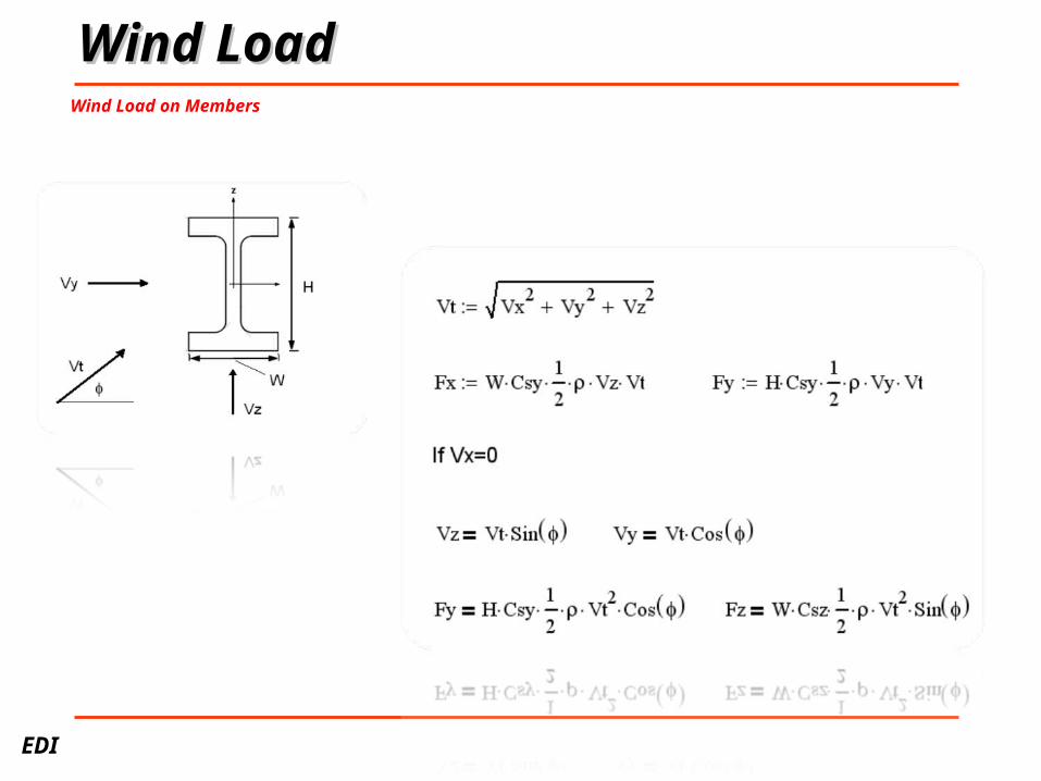
Wind LoadWind LoadWind Load on Members
•

EDI
Wind LoadWind Load
• Wind Load on Inclined Areas/Members
Where : p is pressure A is the total area exposed to wind load in the direction of wind is the angle between the direction of the wind and the axis of the member (or plane of surface)

EDI
Wind LoadWind Load• Wind Areas
Wind areas or are defined to account for the wind loading on un-modeled items such as derricks, buildings, mechanical equipment, flare booms, etc.
A wind area is designated by a two character area identifier and consists of one or more surfaces defined using AREA input lines.
The orientation of the surface is specified either by entering the projections of it on planes normal to the global axis or by specifying the area along with the azimuth and elevation angles.

EDI
Wind Load• Wind Areas
If more then one projected plane is specified for the same area identifier then the resultant area is used.
It is recommended that if an object has projected areas in two or three planes that two separate wind areas be defined rather than specifying two projections together.

EDI
Wind Load• Wind Areas
The surface shape may be designated as flat or round together with a corresponding shape factor.
The wind force components are calculated by multiplying the calculated wind pressure by the shape factor and the projected areas. The wind force is assumed to act at the specified centroid of the surface.
•

EDI
Wind LoadWind Areas
The wind load is distributed over the specified number of joints.
If more than one joint distribution is specified, the program assumes that these joints are connected to a rigid body to which the wind force is applied. The load is distributed to each joint by assuming the rigid body is supported at each joint by three translational and three rotational springs.
The stiffness of the translational springs is unity while that of the rotational springs is 0.01 in the unit system the problem is defined.
Wind Shield Zones
By default, members located above the water surface receive wind loading. The program allows the specification of wind shield zones where members do not receive wind loading.Wind shield zones are defined by specifying the bottom and top elevation of the zone. Elevations are defined using global z elevation.

EDI
Special ElementsSpecial ElementsSACS Special Elements :
Wishbone Elements
Gap Elements : Compression Only Element
Tension Only Element
No Load Element
User defined Load Deflection Element
Friction Element

EDI
Special ElementsSpecial ElementsWishbone Element:
Wishbone Element is a factious element connecting two coincident
joints used to model special boundary conditions between connecting structures.
6 inch
direction of offset
For example : Pile inside leg, conductor guide.
two coincident joints
member end release at one joint 1 0 0 1 1 1 x y z rx ry yz 1
EDI
Special Elements Special Elements
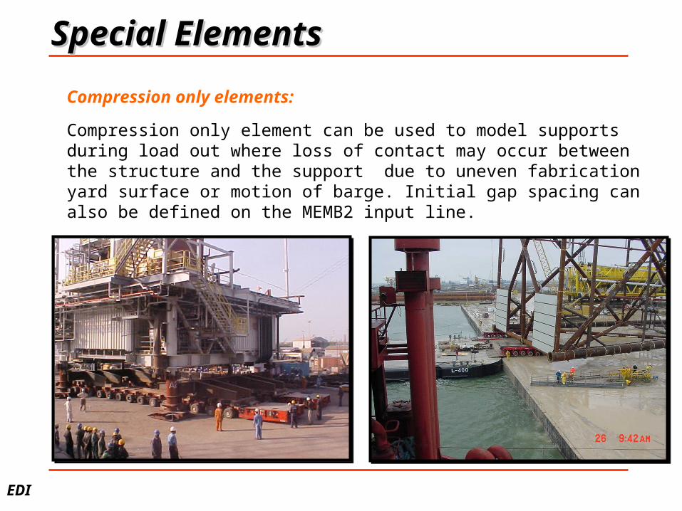
Compression only elements:
Compression only element can be used to model supports during load out where loss of contact may occur between the structure and the support due to uneven fabrication yard surface or motion of barge. Initial gap spacing can also be defined on the MEMB2 input line.

EDI
Special ElementsSpecial ElementsTension only elements:
Tension only elements/ Cable elements can be used to model slings for a
lift analysis in conjunction with moment member end releases. Pre
tension can be defined on the MEMB2 input line.
•

EDI
Special ElementsSpecial ElementsNo Load elements:
No load elements can be used to model tie downs for the pre transportation analysis phase. The no load switch can then be turned off for the transportation analysis and the results from the two can then be combined directly. Same model can be used for both analysis.No load elements can also be used for loadout analysis to model loss of support.

EDI
Special ElementsSpecial ElementsUser defined load-deflection elements:
User defined load deflection elements can be used to define non-linear load deflection characteristics.Many uses: Contact problems, suction pile behavior…etc
P

EDI
Special ElementsSpecial ElementsSpring Elements Any or all degrees of freedom of a joint may be designated as a translation or rotation elastic spring provided that the degree of freedom is designated as fixed (i.e. ‘1’) on the respective joint description line.
When all three translational and/or rotational degrees of freedom are fixed, the support joint coordinate system may be redefined using two reference joints on the ‘Joint Elastic Support’ line. The support joint local X-axis is defined by the support joint and the first reference joint. The local XZ plane is defined by the support joint and the reference joints with the local Z-axis perpendicular to the local X axis.

EDI
Special ElementsSpecial ElementsDented Members Accounts for local indentation and overall deformation. The local dent and the overall deformation are in the direction of member local z direction. The length of the dent is the length of the member or length of segment. The local z can be orientated in any direction using a chord angle or a reference joint. Code check in accordance to modified API equations to account for reduction in cross section and overall deformation as per J.T. Loh paper “Ultimate Strength of Dented Tubular Steel Members”

EDI
Special ElementsSpecial Elements
Super elements: A super element can be defined to be a portion of the structure which has been modeled and reduced down to a set of boundary joints in terms of a reduced stiffness matrix and reduced loads – also known as sub-structuring. Super elements can be useful where: The model is too large for analysis, where portions of the structure are repeated or for linearization of the foundation. Method: The structure is broken down into two portions. The boundary elements on the substructure are defined by boundary conditions of 222222. The same joints exist on the master model with no special boundary conditions. The substructure is reduced using the Superelement module. The super element is imported into the master model during analysis via the super element tab under the analysis options.

EDI
Post - ProcessingPost - Processing• Member Design
– API-WSD
– API-LRFD
– Norsok
– Eurocode
– Danish
– British
– Canadian
– Linear Global (Section 17)
• Joint Design
– API-WSD
– API-LRFD
– Norsok
– Danish
– Canadian
– MSL
– Linear Global (Section 17)

EDI
Post - ProcessingPost - Processing• Element Code Check
K-Factors / Effective Buckling Lengths
• K-factors or effective buckling length, but not both, may be specified for buckling about the local Y and Z axes. K-factors are specified on the pertinent GRUP line in columns but may be overridden on the MEMBER line in columns.
• When K-factors are used, the effective buckling length is calculated as the K-factor multiplied by the actual member length. When effective lengths are specified on the MEMBER line, then the effective buckling length is determined by multiplying the K factor from the GRUP line with the effective length value on the MEMBER line.

EDI
Post - ProcessingPost - Processing• Element Code Check
X Brace K-Factors
For X bracing the K factor for compression elements is 0.9 when one pair of members framing into the joint must be in tension if the joint is not braced out of plane.
•

EDI
Post - ProcessingPost - Processing• Element Code Check
K Brace K-Factors
For K bracing the K factor for compression elements is 0.8 when one pair of members framing into the joint must be in tension if the joint is not braced out of plane.
•

EDI
Post - ProcessingPost - Processing• Element Code Check
Reduction Factor Cm
Cm can be based upon a constant value of 0.85, based upon end moments or axial load calculations or set to 1.0. The various options are defined on the GRUP line on column 47.
Alternatively enter ‘M’ in column 34 of the OPTIONS line to exclude the value of the reduction factor Cm for combined axial compression and bending unity check, or enter ‘C’ to globally set the value of Cb to 1.0
•

EDI
Post - ProcessingPost - Processing• Element Code Check
Cb
The value for Cb for members with Compact or Non-compact Sections with Unbraced length greater than Lb can be taken as 1.0 (default) or based upon end moment calculations as shown below by entering B in column 33 of the OPTIONS line.
•

EDI
Post - ProcessingPost - Processing• Joint Can
API RP2A 21st Edition Supplement 2 guidelines implemented.
Joints checked against API specified validity ranges.
Where validity ranges have been infringed, Joint Can will report the lesser capacity based upon actual geometry or the limiting dimension.
Joint capacities dependant of joint classification (i.e. K, X and Y)

EDI
Post - ProcessingPost - Processing• Joint Can
Basic Capacity of joints without overlap is given by:
Strength Factor Qu varies with the joint and load type (Table 4.3-1 API RP2A 21st Edition Supplement 2)

EDI
Post - ProcessingPost - Processing• Joint Can
Chord Load Factor Qf
Values for C1, C2 and C3 vary by joint type (Table 4.3-2)
FS = factor of safety Pc and Mc are axial and bending moment resultants in chord

EDI
Post - ProcessingPost - Processing• Joint Can
Joints with Thickened Cans
Lc is the chord length. Pa dependent upon chord length (BRCOVR)
where : is the thickened can reduction factor
Tn is nominal chord member thickness Tc is the chord can thickness (Pa)c is axial allowable based upon chord geometric and material properties

EDI
Post - ProcessingPost - Processing• Joint Can
Strength Check Interaction Ratio

EDI
Post - ProcessingPost - Processing• Joint Can
API assumes compression capacity is limited by brace. Joint Can assumes Qu for compression is the same as for tension.
Grouted Joints
The Qf calculation for double skinned joints is based upon the chord thickness T With load sharing between the chord and inner tube accounted for. Implementation to Overlapped Joints Currently under consideration
Ovalization failure capacity estimated by using effective formulation. T=chord thickness, Tp = Inner tube thickness

EDI
Post - ProcessingPost - Processing• Joint Can
Mixed Class Joints For mixed class joints the axial term in the interaction equation can be based upon either interpolation or ratio calculations.
Interpolation
RatioIn which k, x and y are proportions of the classification
EDI
PSI - CapabilitiesPSI - Capabilities
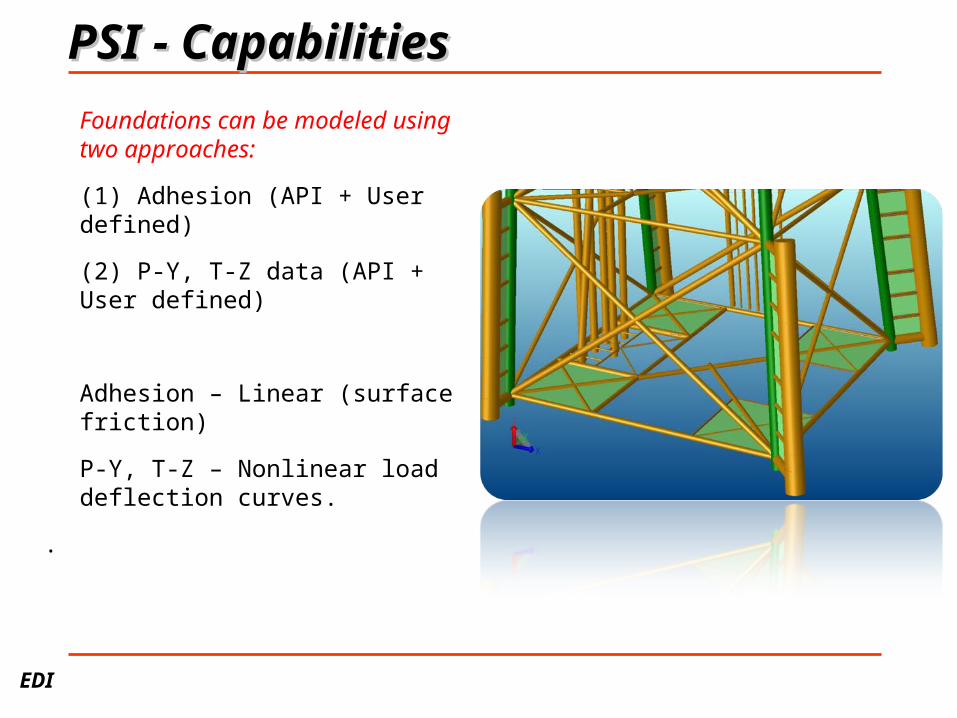
Foundations can be modeled using two approaches:
(1) Adhesion (API + User defined)
(2) P-Y, T-Z data (API + User defined)
Adhesion – Linear (surface friction)
P-Y, T-Z – Nonlinear load deflection curves.
.
EDI
PSI - CapabilitiesPSI - Capabilities
•
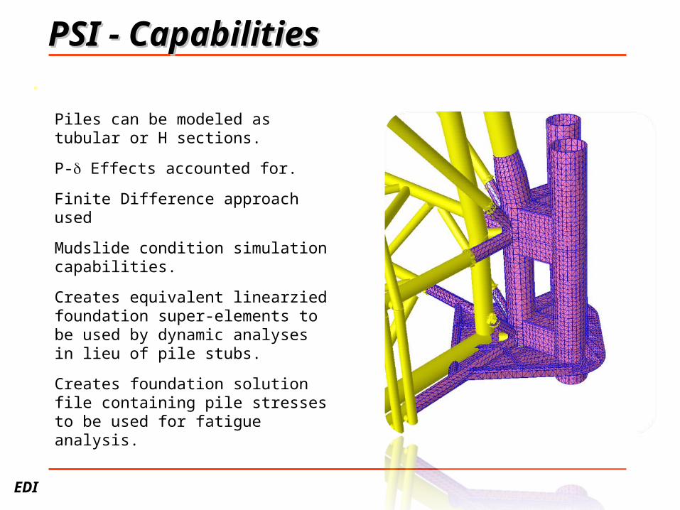
Piles can be modeled as tubular or H sections.
P- Effects accounted for.
Finite Difference approach used
Mudslide condition simulation capabilities.
Creates equivalent linearzied foundation super-elements to be used by dynamic analyses in lieu of pile stubs.
Creates foundation solution file containing pile stresses to be used for fatigue analysis.
EDI
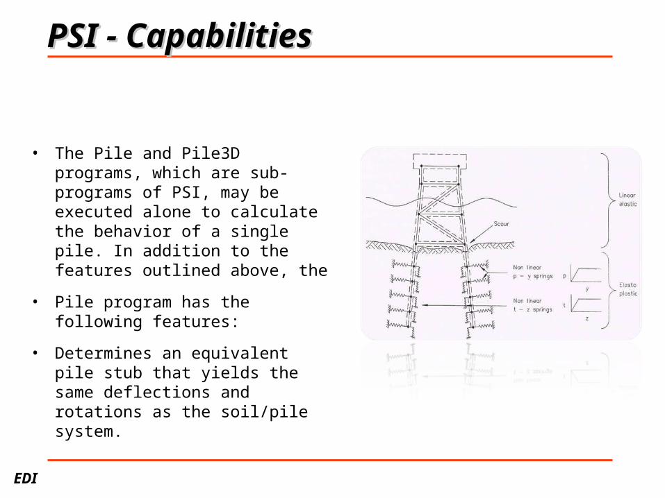
PSI - CapabilitiesPSI - Capabilities
• The Pile and Pile3D programs, which are sub-programs of PSI, may be executed alone to calculate the behavior of a single pile. In addition to the features outlined above, the
• Pile program has the following features:
• Determines an equivalent pile stub that yields the same deflections and rotations as the soil/pile system.

EDI
PSI - ModelingPSI - Modeling
• Pile head Joint
• The interface joints between the linear structure and the nonlinear foundation must be designated in the SACS model by specifying the support condition ‘PILEHD’ on the appropriate JOINT input line. NOTE: The ‘PILEHD’ support condition represents fully fixed condition in lieu of a PSI analysis.
• Pile Local Coordinate System
The pile default local coordinate system is defined with the local X axis pointing upward from the pile head joint along the pile axis defined by the pile batter joint or batter coordinates. By default, the local Y and Z axis orientations are load case dependent. For each load case, the local Y axis is automatically oriented such that it coincides with the direction of maximum pilehead deflection.
The orientation of the local Y and Z axes may be overridden by the user by specifying the rotation angle about the local X axis in columns 51-56 on the PILE line

EDI
PSI - ModelingPSI - Modeling
• Specifying Elevations for Soil Resistance Curves
• Within a soil stratum, the PSI program connects the input P-Y or T-Z points with straight lines to fully define the pile/soil interaction curve for arbitrary displacements in that stratum. At depths between specified soil strata, PSI has the ability to linearly interpolate between curves or to use a constant T-Z curve. Interpolation between different strata may be achieved by omitting the bottom of strata location.

EDI
PSI Solution Procedure (P-Y, T-Z)
The jacket structure is initially reduced to a super element at each pile head.

EDI
PSI Solution Process
Iterative Solution Procedures
Stiffness Table Approximation (5%)
Fine Tune Solution
SOLUTION
EDI
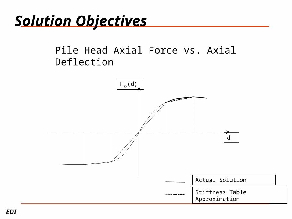
Pile Head Axial Force vs. Axial Deflection
Fax(d)
d
Actual Solution
Stiffness Table Approximation
Solution Objectives

EDI
Stiffness Table Approximation
• Approximate model of the pile head behavior
• Pile head forces are sampled for a range of points
• Linear interpolation between the points
• Reduction of computation time
• Improved chance of solution for highly non-linear problems
• Automatically generated (internal) … OR …
• User-specified with the TABR line
•

EDI
TABR lines
Excerpt from PSI Listing File
*********************** TABR CARD IMAGES ******************* TABR AXIAL DF .0250 .10 PL1 SOL1 TABR DEFLECTN 0. 2.0 5.0 PL1 SOL1 TABR ROTATION -.01500. .0150 PL1 SOL1 TABR TORSION 0. 100.0 PL1 SOL1 TABR AXIAL DF -.0557.44430 PL2 SOL2 TABR DEFLECTN 0. 2.0 5.0 PL2 SOL2 TABR ROTATION -.01500. .0150 PL2 SOL2 TABR TORSION 0. 100.0 PL2 SOL2
TABR AXIAL LD -7500. 0. 7500. PL3 SOL3
Axial Adhesion Model
cm/in
rad
kips-ft/kN-m
cm/in
kN/kips
EDI
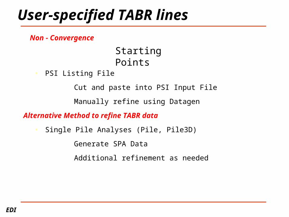
User-specified TABR lines
• PSI Listing File
Cut and paste into PSI Input File
Manually refine using Datagen
• Single Pile Analyses (Pile, Pile3D)
Generate SPA Data
Additional refinement as needed
Starting Points
Non - Convergence
Alternative Method to refine TABR data

EDI
PSI Convergence Tolerances
Iterative Solution Procedures
Stiffness Table Approximation
Fine Tune Solution
SOLUTION
Force Tol. (0.5%)
Deflection Tol. (5%)
Rotation Tol (0.0001)
Deflection Tol (0.001)

EDI
Convergence Report
** ITERATION DATA FOR LOAD CASE XXXX **
ITERATION RMS DEFLECTION RMS ROTATION
1 0.039673 0.000027
2 0.001083 0.000003
3 0.000070 0.000000
MAXIMUM PILEHEAD FORCE DIFFERENCE= 7.53085 %
4 0.022679 0.000026
MAXIMUM PILEHEAD FORCE DIFFERENCE= 7.67680 %
5 0.000626 0.000001
MAXIMUM PILEHEAD FORCE DIFFERENCE= 0.35047 %
Excerpt from PSI listing file
• Stiffness Table Approximation • Fine Tune Solution

EDI
Trouble Shooting – A checklist
• Review convergence report
• If necessary, use TABR lines
• Check tolerances and controls
• Review soil data
• Investigate each pile using Single Pile Analysis
• Fully constrain the pile heads and run SACS

EDI
Future Developments
• Shallow Foundations
Spud-can Foundations
Soil Plasticity Models (Collapse only)
• API RP 2A-WSD /21 Supplement 3
CPT Methods (loose soils, dense silt)
Scour Depth Guidelines

EDI
Solution Objectives (lateral)
Fz(dz,θ)
θ
dz
Actual Solution
Stiffness Table Approximation
Lateral Pile Head Force vs. Lateral Deflection and Rotation

EDI
PSI/Pile Module
• PSI Utilities
Plot Soil Data
Plot Pile Capacity
Plot Pile Load

EDI
Grouted Joints – Joint Can
The following technique is used to determine the internal loads of a leg. 1.The internal moment in the leg is determined by ratio the moment of inertia of the combined section to that of the leg only.
2. Similarly, the axial load in the leg is based upon the ratio of the combined section area to that of the leg only.

EDI
Grouted Joints – Joint Can/Fatigue
The following methods are available for determining the effective thickness of a leg for joint can and fatigue analysis. 1. Effective thickness based upon moment of inertia of composite section

EDI
Grouted Joints – Joint Can/Fatigue
The following methods are available for determining the effective thickness of a leg for joint can and fatigue analysis. 2. Effective thickness based upon moment of inertia of the walls instead of composite section.

EDI
Grouted Joints – Joint Can/Fatigue
The following methods are available for determining the effective thickness of a leg for joint can analysis. 3. Square root of the sum of the squares of the leg and pile thickness.
EDI
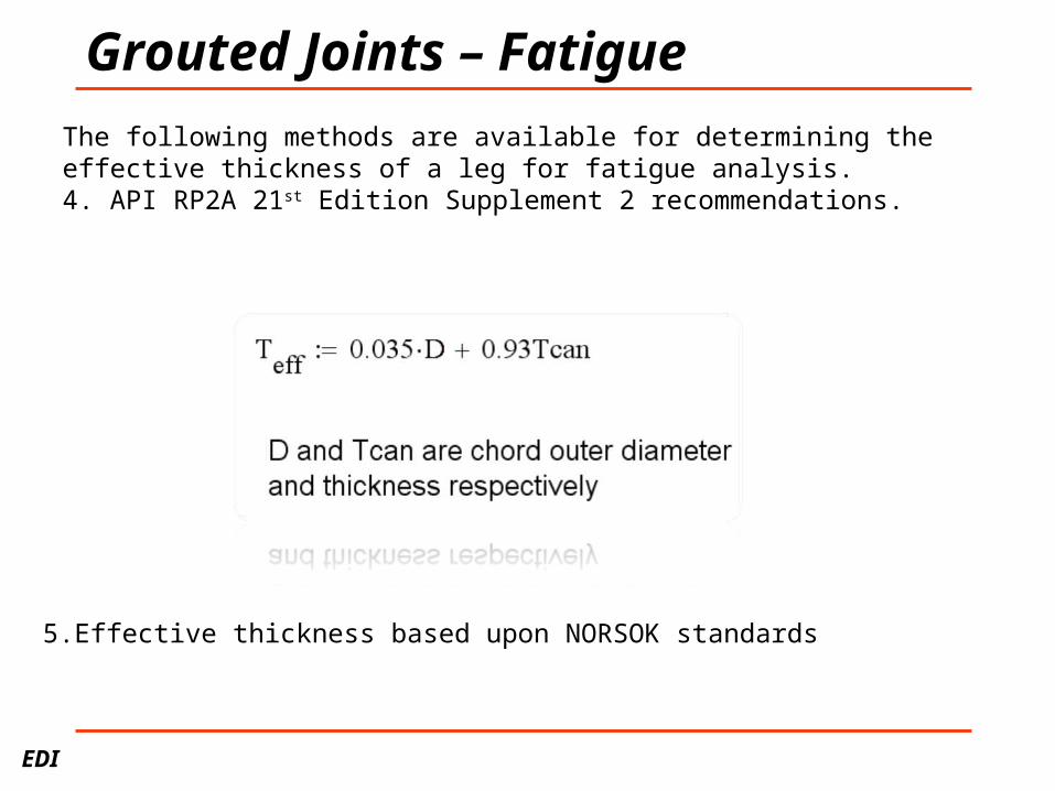
Grouted Joints – Fatigue
The following methods are available for determining the effective thickness of a leg for fatigue analysis. 4. API RP2A 21st Edition Supplement 2 recommendations.
5.Effective thickness based upon NORSOK standards

EDI
Ring Stiffened Joints – Fatigue
SCF’s factored using Smedley and Fisher ring stiffened formulation. The RING input line may be used to define the ring dimensions and the ring group. The ring stiffened connection input line CONRST may be used to apply the rings to a particular brace and the location of the ring.

EDI
Modal Extraction : DYNPAC• Some of the main features and capabilities of the DYNPAC MODULE are:
Determines Natural Frequencies
and modes of vibration.
Accounts for structural mass and
fluid added mass automatically
Supports lumped or consistent
mass generation
Determines modal mass
• participation to allow determination
of number of modes required for
subsequent forced dynamic analysis.

EDI
Modal Extraction : DYNPACAnalysis Procedure:
Linearize Foundation (Pile Superelement)
- identify load cases for pile linearization, load cases dependent upon type
of analysis.
- include dead load
- run PSI to generate Pile superelement.
Modal Analysis
- specify retained degrees of freedom.
- Identify load cases to be converted to mass.
- check cumulative mass participation factors.
- check natural frequency and period (dynamic response low if period less
that 2 seconds)

EDI
Load Path Dependent SCF’s
For any tubular connection, all braces that lie in a plane with the Chord or within 15
degrees of that plane are considered in the calculation of load path SCF’s
The chord member is selected on the following hierarchy:
1. Largest diameter
2. Largest wall thickness
3. Highest Yield stress
4. Members that are in-line with a 5 degree tolerance

EDI
Load Path Dependent SCF’s
Joint Classification
KT-connection: Axial load in middle brace opposes axial load from outside brace.
For a KT connection the load to be transferred is taken as the
smallest value of:
1) Center brace axial load
2) Twice the axial load component
normal to the chord.
The KT percentage for each brace is ratio of the
transferred KT normal axial load component and the
original axial load value.
The remaining axial loads are then considered for
K joint load transfer.

EDI
Load Path Dependent SCF’sJoint Classification
For a K joint the axial load component normal to the chord is balanced by the axial
load component normal to the chord in other braces (on the same side of the
chord).
The brace with the smallest normal axial load component is considered first with
the brace containing the largest opposing normal axial load component.
The balanced load is subtracted from the opposing brace and the process is
repeated until all K joints are identified.
Any X joint load paths are considered next for braces on opposite sides of the
chord. The largest opposing normal axial force is considered first. The balanced
load is subtracted from opposing brace and the process is repeated until all X joints
are identified. Braces with remaining unbalanced axial loads are treated T/Y joints.

EDI
Load Path Dependent SCF’s
SCF Determination
The load path dependent SCF is calculated as a weighted average of the
applicable KT, K, X and TY joints as:
SCF = RKT*SCFKT+ RK*SCFK + RX*SCFX + RTY*SCFTY
where RKT, RK , RX , and RTY are the ratios of each type of joint action.

EDI
Importing FE Joint MeshJoint Meshing
Two approaches are available for importing meshed joints into a SACS ‘stick’ model.
1. FEMGV
Precede can generate a FEMGV batch file once a joint has been isolated by inserting
a joint on the braces and chord members to define the portion of the joint that needs
to be meshed. Precede will require the joint name, the number of elements around
the circumference of a brace with the smallest diameter and also the element type.
The batch file can then be subsequently read into FEMGV and the mesh is generated
automatically.
FEMGV can generate a FEMGV neutral file which can be read back into Precede and
the mesh can be incorperated into the rest of the model by tools provided in Precede.

EDI
Importing FE Joint MeshJoint Meshing (Continued)
2. SACS Mesh Joint Utility
Very simple to use. Provide joint name to mesh, the mesh intensity ( limits 0.5 – 2, mesh
intensity 1 = approx 28 nodes around the circumference of the smallest brace) and the model
file name.
The mesh utility will automatically mesh the joint and output a OCI file containing the ‘stick’
model with the joint mesh incorporated.
FEMGV - Mesh Joint Utility
FEMGV allows the user to control the length of brace/chord to be meshed. Also gives choice of
element types. Cannot mesh joints with overlapped braces.
Mesh Joint Utility allows the meshing of overlapped joints. No user control over the length of
brace/chord member to be meshed. Meshing restricted to triangular palte elements (this is not a
disadvantage).

EDI
Fatigue AnalysisFatigue Analysis• Fatigue analysis is required due to the cyclic loading imposed on the Jacket tubular joints by
wave loads.
• Fatigue analysis could be of two types: : Deterministic Fatigue
Spectral Dynamic Fatigue
• SCF for tubular joints are based on SCF for tubular joints are based on parametric equations available for the parametric equations available for the class of joint under consideration.class of joint under consideration.
• Number of cycles to failure NNumber of cycles to failure N ii is is
obtained from the S-N curve. obtained from the S-N curve.
• S-N curve used is selected based on S-N curve used is selected based on the particular weld detail.the particular weld detail.

EDI
Fatigue AnalysisFatigue Analysis
• In Deterministic FatigueDeterministic Fatigue, discrete number of waves are used to
characterize the total fatigue environment
• Partial Damage from the sea state =
• Damage is accumulated over all sea states (Miners LawMiners Law):
•
•
• Deterministic analysis has been done for many years and has proven to be a reliable approach for dynamically insensitive structures, and for situations where all fatigue waves are of sufficiently long wave periods to avoid peaks and valleys of the structures transfer function.
• Very sensitive to the waves chosen for the analysis
i
i
N
n
..........N
n
N
n
N
n
N
n
3
3
2
2
1
1
i
i
i
D

EDI
Fatigue AnalysisFatigue Analysis
• The spectral fatigue approach utilizes wave spectra and transfer functions, thus allowing the relationship of the ratio of structural response to wave height as a function of wave frequency to be developed for the wave frequency range. Therefore spectral fatigue accounts for the actual distribution of energy over the entire wave frequency range.
• In Dynamic Spectral Fatigue , Spectrum used to define the fatigue
environment are:
• JONSWAP
• Ochi-Hubble
• Pierson-Moskowitz
• These Spectra are in-built in SACS
•

EDI
Fatigue AnalysisFatigue Analysis•Fatigue program features are as below
• Includes a wide range Stress Concentration Factor Includes a wide range Stress Concentration Factor (SCF) th(SCF) theories and allows user defined input.
• Automatic redesign of chords or braces may be done to determine required joint can or brace stub thickness
• API, AWS and NPD fatigue failure (S-N) curves are built into the program. Also allows user defined input.
• • Generates output for the Interactive Fatigue Module for Interactive redesign.Generates output for the Interactive Fatigue Module for Interactive redesign.
J182 J186-J182 TUB 45.7 1.0 K BRC 3.74 5.03 4.76 4.74 4.84 0.26334 B 94.93
J182 JF2-J182 TUB 55.9 2.5 K CHD 3.74 2.31 1.88 1.88 1.99 3.70E-03 T 6,763.51
Chord
Len.(m)
Out of
Plane
Service
Life
Stress Concentration Factors
OD(cm)
WT (cm)
Joint
Type
Member
Type
Original Dimensions
Joint Member Type ID Inplane Damage LocationAxial
(Crown)
Axial
(Saddle)
MEMBER FATIGUE REPORT (DAMAGE ORDER)

EDI
Dynamic Spectral FatigueAnalysis Procedure:
Linearize Foundation
-choose load cases for developing foundation superelement
Modal Analysis to generate mass and mode files
- check cumulative mass participation factors
Run Wave Response to generate Transfer Function for each direction.
- use waves of constant steepness to generate transfer function.
- avoid waves under 1 foot ( 30cm )
- check transfer function for overturning moment and base shear.
- solve for equivalent static loads.
Run Fatigue
- choose appropriate spectrum
- choose S-N and SCF options

EDI
Earthquake AnalysisTwo approaches available: 1)Response Spectrum:
A response spectrum depicts the maximum response to a ground motion of a series of single degree of freedom oscillators having different natural periods but the same amount of internal damping.
2) Time History Time History is a continuous record of ground motion or response.

EDI
Earthquake AnalysisAnalysis Method:
1. All support points are assumed to be moving with the ground.
2. Each mode of vibration is assumed to act as a single degree of freedom.
3. Solve equations of motion for each mode.
4. The response from each mode for each direction (X, Y and Z) is combined using the SRSS (Square Root of the Sum of Squares) method to obtain the multi directional response. The SRSS approach is used on the assumption that the responses from different directions are uncoupled
5. The response for each mode in each direction is also combined using the CQC (Completer Quadratic Combination) method. For the cases where there is sufficient modal separation in different directions the CQC method devolves into the SRSS approach.

EDI
Earthquake AnalysisAnalysis Method: 6. The dynamic response program creates a common solution file containing end forces, stresses, reactions and displacements. Because these results are obtained by combining modal results using RMS techniques, end forces, stresses…etc. have no sign associated with them and are taken as all positive values. 7. The dynamic response generates two sets of load cases for both the member check and the joint check.
8. The seismic results are then combined with the results from a static analysis. This is followed by element code check and joint can check.
EDI
Earthquake AnalysisDamping: Damping effects are important and for structure immersed in fluid the damping is a nonlinear effect since damping is a function of the amplitude of response. Three options for damping available.
1.Linear modal damping. (API recommends overall modal damping of 5% (SDAMP line)
2. User defined amplitude to be used in fluid damping calculation (FDAMP line).
3. Program will calculate through iterative technique as follows (FDAMP line): (a)Calculate the response based upon an assumed amplitude.
(b) Calculate equivalent fluid damping based upon this response.
(c) Repeat this process until the response until the response amplitude agrees with the amplitude used for equivalent fluid damping.

EDI
Earthquake AnalysisStrength Requirements:
G is the ratio of the effective horizontal ground acceleration to gravitational acceleration.
Using the response spectrum, the ordinates of the spectrum shouldbe multiplied by the factor G forthe zone in which the platform islocated. The resulting spectrum should beapplied equally along both principalhorizontal axis and one half in the Vertical direction. All three spectrashould be applied simultaneously andresponses combined using CQCmethod.

EDI
Earthquake Analysis Strength Requirements:
The strength requirements are intended ensure that no significant structural damage can occur due to a strength level earthquake. For strength level earth quake both the member check and joint check allowables may be increased by 70 percent.
Tubular Joints
Joints for the primary structural members should be sized for either the tensile yield load or the compressive buckling load of the brace.

EDI
Earthquake Analysis Strength Requirements:
Tubular Joints – calculation of allowables.
The punching shear stress allowable, vpa is :
The factor Qf is given by :
In which the factor A is computed as :
Where fAX, fIPB and fOPB are stress in the chord due to twice the strength levelseismic loads in combination with gravity, buoyancy, hydrostatic pressure or or the full capacity of the chord away from the joint can – whichever is the less.whichever is the less.

EDI
Earthquake Analysis Strength Requirements:
Tubular Joints – calculation of unity check
For combined axial and bending stresses in the brace the followinginteraction equation should be satisfied:
For earthquake analysis the terms corresponding to bending areignored since we are checking against the tensile yield loads or thecompressive buckling load of the brace. Joint can requirements for a earthquake analysis can be activated by specifyingthe EQK option on the JCNOPT line and also by specifying 2.0 for the jointload case factor on the STCMB line.

EDI
Earthquake AnalysisDuctility Requirements
Rare Intense Earthquake:
In seismically active areas, rare intensive earthquake motion may involve inelastic action and structural damage may occur. The ductility requirements are intended to ensure that the structure and the foundation have enough reserve capacity to prevent collapse in the event of a rare intense earthquake.
Equivalent Static Loads: The Dynamic response module can output equivalent static loads corresponding to The modal responses being combined to generate the highest amount of base shear or overturning moment in 20 directions (every 18 degrees)

EDI
Earthquake AnalysisDesign Criteria:
Equivalent Static Loads: The Dynamic response module can output equivalent static loads corresponding to the modal responses being combined to generate the highest amount of base shear or overturning moment in 20 directions (every 18 degrees).
For rare intense earthquakes the equivalent static loads can be used to design the foundations and also conduct an elasto-plastic analysis of the structure to design against failure.

EDI
Earthquake AnalysisDesign Criteria:
Low-level Earthquake: For areas where the ground acceleration is less than 0.05g no earthquake analysis is required. For areas where the ground acceleration is between 0.05g – 0.1g a low level earthquake analysis is required. The joint check requirements for a low level earthquake are the same as those for an in-place analysis.
The joint can requirements for a low-level earthquake analysis can be activated by specifying LLEW option for API working stress design , LLEL for API LRFD design on the JCNOPT line and also by using the DLOAD load line in the Joint can input file to identify the dead load case used in static analysis.

EDI
Spectral Wind FatigueMethod: 1.Conduct modal extraction analysis – determine mode shapes and natural frequencies. 2. 2. Each mode of vibration is assumed to act as a single degree of freedom. 3.Determine Mechanical Transfer function H(f) for each mode.
where Ki is the generalized stiffness matrix, fn is the natural frequency and c is percent damping.

EDI
Spectral Wind FatigueMethod (continued): 4. Determine RMS response for each mode. where Si(f) is the Harris spectrum given by:
where LH is the reference length (1800m), k is the surface roughness coefficient (0.0025) and v10 is the wind speed at 10m reference height.

EDI
Spectral Wind FatigueMethod (continued): 5. The response for each mode is combined to obtain the total response using the CQC (Completer Quadratic Combination) method.
where I and k refer to the ith and the kth mode and Pik is the modal correlation coefficient.

EDI
Spectral Wind FatigueMethod (continued): 6. Wind velocities are assumed to conform to the Weibull distribution. Wind velocities are selected to define the Weibull distribution time slices and velocity ranges for integration limits to calculate fraction of occurrence.
EDI
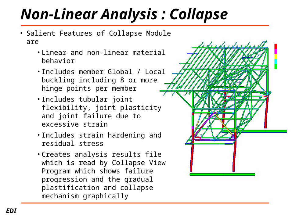
Non-Linear Analysis : Collapse• Salient Features of Collapse Module are
• Linear and non-linear material behavior
• Includes member Global / Local buckling including 8 or more hinge points per member
• Includes tubular joint flexibility, joint plasticity and joint failure due to excessive strain
• Includes strain hardening and residual stress
• Creates analysis results file which is read by Collapse View Program which shows failure progression and the gradual plastification and collapse mechanism graphically

EDI
Pushover Analysis• Pushover Analysis conducted to determine the
reserve strength ratio of a jacket structure.
Loading applied to the structure in sequence.
Apply all gravity loads first.
Apply environmental storm loading.
Increase magnitude of environmental loading until the structure fails.
RSR = Base Shear at 100% storm Load Base Shear at Failure
Other approaches define failure with
100, 500, 1000, 5000,…year storms
First Failure

EDI
Ship Impact Analysis is carried out to determine the
Reserve Strength in the structure after the collision.
Vessel mass, added mass coefficient and velocity at
the time of collision is specified on ENERGY line.
Impact load case and impact joint defined on
IMPACT input line.
Run Collapse – impact load will be applied until all
kinetic energy is absorbed. The structure will then
automatically unload and the post impact loading
can be applied.
SACS can optionally account for vessel
deformation. Local indentation energy can be
accounted for by either meshing the impacted
member or using API methodology.
Ship Impact Analysis (Static)

EDI
Dynamic Response
Force Driven Analysis Force time history, Periodic and Engine vibration analyses are supported. The main capabilities and features for force driven analysis are detailed below: Force Time History 1. Linear, quadratic, or cubic interpolation available for the time history input. 2. Automatic load case selection based on overturning moment, base shear, joint displacement, etc. 3. Variable time step integration procedure. 4. Time history plots including modal responses, overturning moments, base shear, etc. 5.Generation of equivalent static loads for force/time history collapse analysis.

EDI
Blast AnalysisBlast Analysis
Large Deflection, Elasto-Plastic Non- Large Deflection, Elasto-Plastic Non- Linear Finite Element Analysis is performed Linear Finite Element Analysis is performed
in SACS for Blast loads. in SACS for Blast loads.
Blast Resistant Design to minimize the risk Blast Resistant Design to minimize the risk
to people and facilities from the hazards of to people and facilities from the hazards of accidental explosions. accidental explosions.
Dynamic Response Module can be used to Dynamic Response Module can be used to
apply blast load profile to the structure at apply blast load profile to the structure at
discrete time steps.discrete time steps.
Dynamic Response

EDI
Blast Analysis (continued)
Dynamic Response will generate a structural output file
containing incremental loading (including dynamic and
static components).
Dynamic Response will also output a load sequence
file for Collapse.
Run Collapse for non-linear elasto-plastic
analysis using incremental loading.
Collapse shows plasticity over time
with each load step representing a
time increment.
Dynamic Response

EDI
Dynamic Ship Impact Use Dynamic Response module to determine dynamic
structural response due to impact.
Set analysis option to SHIP on the DROPT line.
Define vessel mass, velocity, direction of motion and
the impact joint on the SHIP input line.
Define the time history source as SHIP on the time
history load line THLOD.
Prepare Collapse input with control parameters
and load sequence for dead loads.
Run dynamic response.
Dynamic will output Collapse load sequence
and incremental loading containing dynamic
and static components of the structural
response
Dynamic Response

EDI
Dynamic Response
Earthquake/Base Driven Analysis Both spectral earthquake and time history earthquake analyses are supported. Some of the seismic analysis capabilities follow: Spectral Earthquake 1. API response spectra are built into the program. 2. Supports user defined response spectra. 3. Spectral motion can be described as acceleration, velocity, or displacement. 4. Modal combinations using linear, SRSS, peak plus SRSS, or CQC methods. 5. Ability to use a different response spectrum for each direction. 6. Combines seismic results with static results automatically.

EDI
Dynamic Response
Earthquake/Base Driven Analysis Time History Earthquake 1. Includes earthquake time history libraries. 2. User defined input time histories. 3. Linear, quadratic, or cubic interpolation available for the time history input. 4. Variable time step integration procedure. 5. Automatic load case selection based on overturning moment, base shear, etc. 6. Graphical representation of output variables.

EDI
Dynamic Response
Engine/Compressor Vibration 1.Supports mechanical unbalanced forces and gas torques in addition to reciprocating loads. 2. Linear and/or nonlinear interpolation of forces between running speeds. 3. User can select specific joints to monitor or monitor all joints. 4. Allows user defined phasing of forces and moments within a load case. 5. Can automatically combine maximum response of various load cases. 6. Generates plots of input data versus time for any load case. 7. Calculates periodic forces amplitudes and periods from force versus time input.

EDI
Dynamic Response
Spectral Wind Analysis The wind spectral fatigue and extreme wind analyses are supported. Some of the spectral wind analysis capabilities are as follows: Extreme Wind 1. Determines dynamic amplification factors automatically. 2. Generates common solution file containing internal loads, stresses, reactions and displacements multiplied by its own dynamic amplification factor. 3. Includes cross correlation of modal responses using the Complete Quadratic Combination (CQC) modal combination technique. 4. Plots generalized force spectrum and response spectrum for each wind speed. 5. Uses Harris Wind spectrum.

EDI
Dynamic Response
Spectral Wind Analysis The wind spectral fatigue and extreme wind analyses are supported. Some of the spectral wind analysis capabilities are as follows: Wind Fatigue 1. Uses Harris Wind spectrum. 2. Optionally creates Fatigue input file automatically. 3. Distributes wind speed utilizing a Weibull distribution. 4. Assumes Rayleigh distribution of RMS stresses. 5. Handles multiple wind directions in same analysis execution.

EDI
Dynamic Response
Ice Force Analysis Ice Vibration The ice vibration analysis capability includes the following features: 1. Automatically includes ice stiffness. 2. Maximum and minimum peak selection. 3. Automatic cycle count for fatigue analyses. 4. Creates fatigue input data automatically. 5. Full plot capabilities including ice forces, modal responses, overturning moments, base shear, etc. 6. Variable time step integration procedure.