Basics of RF Ampliﬁ er Measurements with the E5072A ENA ... · Basics of RF Ampliﬁ er...

Basics of RF Amplifi er Measurements with

the E5072A ENA Series Network Analyzer

Application Note

The RF power amplifi er is a key component used in a wide variety of industries

such as wireless communication systems, medical equipments, and aerospace

and defense areas. Characterizing the basic performance of the amplifi ers is a

critical stage in the R&D or manufacturing test environments. These amplifi ers

must meet strict performance specifi cations in order that the systems can

comply with regulations.

This application note illustrates how to setup fundamental amplifi er measure-

ments such as S-parameters, K-factor gain compression, harmonic distortion

or pulsed measurements with a simple confi guration using a vector network

analyzer (VNA). Some advanced techniques using the Agilent E5072A ENA

Series Network Analyzer 1 will be covered in the note with step-by-step instruc-

tions of typical amplifi er characterization.

1. See the E5072A technical overview, product number 5990-8004EN for more detail about the

E5072A.

Introduction

2

Contents

Introduction ................................................................................................................. 1

Characterizing RF Amplifi ers

S-parameter/Stability factor ............................................................................. 3

Full 2-port correction for high-power amplifi er.............................................. 6

Gain with leveled output power ....................................................................... 8

Gain compression ............................................................................................. 15

AM-to-PM conversion ...................................................................................... 16

Harmonic distortion .......................................................................................... 20

Pulsed Measurement ....................................................................................... 27

Summary .................................................................................................................... 32

Appendix A. Power Handling Consideration ..................................................... 33

Appendix B. Amplifi er Measurement Wizard .................................................... 34

Appendix C. Comparison with the E5071C ......................................................... 35

3

Figure 1. Internal source attenuators for uncoupled power.

S-parameters/stability factor

Traditionally, S-parameters (both refl ection and transmission) measurements

have been performed with VNAs. As well as basic S-parameters of devices,

designers and manufacturers have to carefully look into various parameters

calculated from the S-parameters. K-factor is one of the examples and a signifi -

cant parameter especially for amplifi er designers. This factor can be calculated

from all the S-parameters of two-port devices (S11 to S22), and represents the

stability of amplifi ers. When K-factor is greater than 1 while delta is smaller than

1, the amplifi er is unconditionally stable and no oscillation is expected for any

load.

Since K-factor requires all four S-parameters of devices under test (DUT), full

2-port calibration is necessary for most accurate measurements. Full 2-port

calibration uses all four S-parameters, thus it is critical to make sure that all the

S-parameters are accurate.

For measurements of high-gain amplifi ers, external attenuation on the output

port is often required to protect the VNA’s receivers from damage, which

degrades system dynamic range of reverse measurements such as S12 or S22.

The E5072A has two built-in source attenuators on each port and the attenua-

tion can be changed independently, allowing for uncoupled power level for port

1 and port 2. Uncoupling port power is useful for setting a very low source signal

from port 1 and eliminating additional external attenuator on port 2 to improve

dynamic range, which can also improve accuracy of reverse measurements and

a K-factor calculated from all S-parameters. The block diagram of the E5072A

in Figure 1 indicates the independent source attenuators for uncoupled power.

Different power level can be set for each port by selecting different attenuation

of the internal attenuator for the port.

2 2 211 22

12 21

11 21 12 21

1 – S – S +K =

2 S S

where

= S S – S S

Δ

Δ

R1

A

R2

B

High-gain amp

–85 dBm 0 dBm

ATT = 40 dB(Port 1)

ATT = 0 dB(Port 2)

Characterizing RF Amplifi ers – Measurement Parameters

4

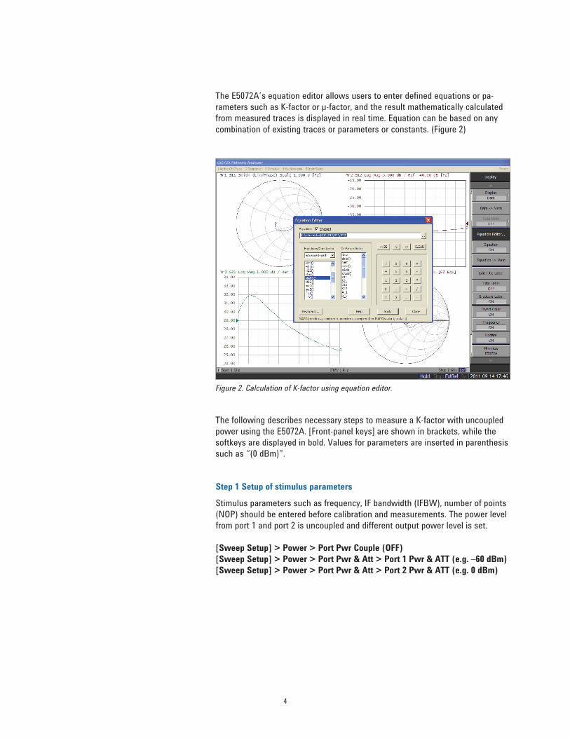
Figure 2. Calculation of K-factor using equation editor.

The E5072A’s equation editor allows users to enter defi ned equations or pa-

rameters such as K-factor or μ-factor, and the result mathematically calculated

from measured traces is displayed in real time. Equation can be based on any

combination of existing traces or parameters or constants. (Figure 2)

The following describes necessary steps to measure a K-factor with uncoupled

power using the E5072A. [Front-panel keys] are shown in brackets, while the

softkeys are displayed in bold. Values for parameters are inserted in parenthesis

such as “(0 dBm)”.

Step 1 Setup of stimulus parameters

Stimulus parameters such as frequency, IF bandwidth (IFBW), number of points

(NOP) should be entered before calibration and measurements. The power level

from port 1 and port 2 is uncoupled and different output power level is set.

[Sweep Setup] > Power > Port Pwr Couple (OFF)

[Sweep Setup] > Power > Port Pwr & Att > Port 1 Pwr & ATT (e.g. –60 dBm)

[Sweep Setup] > Power > Port Pwr & Att > Port 2 Pwr & ATT (e.g. 0 dBm)

5

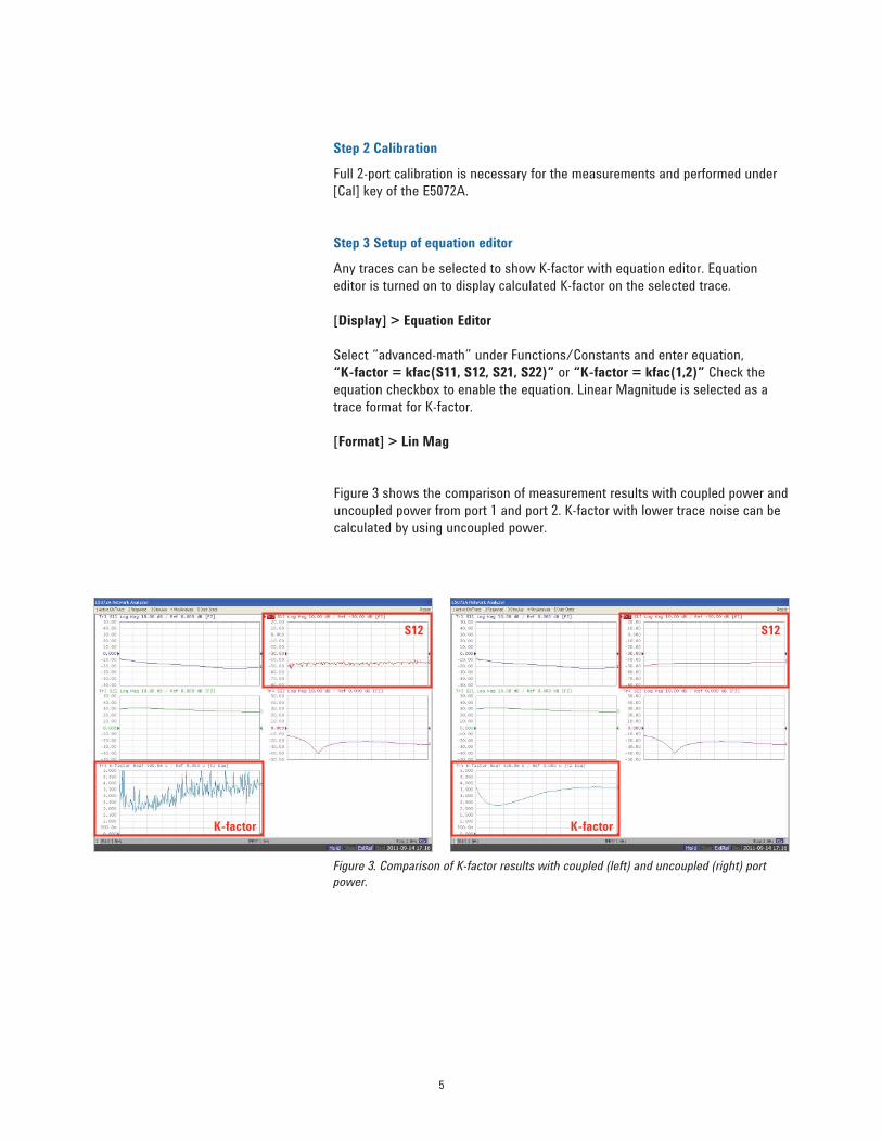
Figure 3 shows the comparison of measurement results with coupled power and

uncoupled power from port 1 and port 2. K-factor with lower trace noise can be

calculated by using uncoupled power.

Figure 3. Comparison of K-factor results with coupled (left) and uncoupled (right) port

power.

Step 2 Calibration

Full 2-port calibration is necessary for the measurements and performed under

[Cal] key of the E5072A.

Step 3 Setup of equation editor

Any traces can be selected to show K-factor with equation editor. Equation

editor is turned on to display calculated K-factor on the selected trace.

[Display] > Equation Editor

Select “advanced-math” under Functions/Constants and enter equation,

“K-factor = kfac(S11, S12, S21, S22)” or “K-factor = kfac(1,2)” Check the

equation checkbox to enable the equation. Linear Magnitude is selected as a

trace format for K-factor.

[Format] > Lin Mag

S12

K-factor

S12

K-factor

6

Full 2-port correction for high-power amplifi er

When designing amplifi ers, it is always important to pay attention to stability

in both small and large signal operation. Not only small signal stability but

large signal stability should be monitored to secure stability of amplifi ers under

real operation. When testing high-power amplifi ers, output power of the DUT

can exceed input compression level or damage level of the internal receivers;

large attenuation should be placed on the output port to protect receivers. The

problem is the large attenuation degrades signal-to-noise (S/N) ratio of reverse

measurements such as S12 or S22 with full 2-port correction. Especially for

refl ection measurements on DUT’s the output port (S22 = B/R2), the source

signal from the analyzer’s port 2 will go through the attenuation, and refl ected

signal from the DUT must go through the attenuation again to reach the receiver

B. This degrades measurement accuracy signifi cantly. The measurement

confi guration is shown in Figure 4.

To solve this problem, the E5072A with a confi gurable test set provides access

to the signal paths between the internal source, receivers, bridges, and the

analyzer’s test ports. The alternative confi guration using the direct receiver ac-

cess is illustrated in Figure 5. For forward measurements such as S21 (= B/R1),

The DUT’s output signal is measured at the receiver B via external coupler, and

appropriate attenuation for protecting the receiver can be selected and inserted

in the receiver path. Isolators with high isolation will attenuate the signal to the

port 2 for protection of the analyzer from damage of high-power input.

For reverse measurements such as S12 (= A/R2) or S22 (= B/R2), the S/N

ratio can be improved by low-loss isolators inserted in the source path from the

port 2 compared to the confi guration with large attenuation in Figure 4. More

accurate S12 or S22 measurements can be performed with the confi guration.

Figure 4. Measurement result of a high-power amplifi er with a

typical confi guration with large attenuation.Figure 5. Measurement result of a high-power amplifi er with a

confi guration using direct receiver access.

S11 S12

S21 S22

S11 S12

S21 S22

7

The power level of measurement example using the both configurations is pre-

sented in Figure 6. The comparison is given for measurements of a high-power

(+30 dBm) amplifier. When the typical configuration using large attenuation is

selected (left), input power level of the receiver B for reverse measurements is

attenuated down to –86 dBm because of large attenuation in the DUT’s output

path. This very small power level results in degraded measurement accuracy

for reverse measurements. Whereas input power level at the receive B can be

optimized (e.g. -50 dBm) by selecting appropriate components in the configura-

tion using direct receiver access (right). Note that higher input power level can

be applied to the DUT for reverse measurements, which improves the S/N ratio

and measurement accuracy for S12 and S22.

Figure 6. Comparison of power level using the confi guration with large attenuation (left) and the confi guration using direct

receiver access (right).

Reverse measurement

Forward measurement

R1

A

R2

B

DUTisolatorcoupler

30 dB ATT

30 dBm 10 dBm

–20 dBm–50 dBm

–26 dBm–86 dBm

10 dBm–20 dBm

R1

A

R2

B

30 dB ATT

0 dBm 30 dBm

0 dBm0 dBm

–60 dBm

DUT

–30 dBm

0 dBm

Reverse measurement

0 dBm

0 dBm

Forward measurement

0 dBm

0 dBm

8

Gain with leveled output power

Some power amplifi ers are tuned and characterized when they are in saturation.

The output level across specifi ed frequency range needs to be very fl at at a

desired constant value, with less than 0.1 dB deviation across the band. Since

the amplifi er’s gain varies across the band, external power leveling of output

power to account for the gain variation is necessary for device characterization.

Conventionally this type of test has been made with a combination of a signal

generator, a power meter and spectrum analyzer. The simple test confi guration

is shown in Figure 7. The DUT’s output power is monitored by a power sensor

via coupler, and the source power from signal generator is adjusted to achieve

target power level of the DUT’s output. Since this power leveling sequence

requires that all the measurement instruments are controlled by a system

controller and measurements have to be synchronized for each data point,

total measurement process takes long time to complete. Also overall cost of

test system with multiple instruments for calibration and repair becomes very

expensive.

Figure 7. Conventional test confi guration for power leveling.

SASG

Power

sensor

System controller

Coupler

Source power is adjusted.

DUTPin Pout

i.e. GPIB

9

The E5072A has capabilities of power calibration techniques for accurate

measurements which offer the replacement to legacy test systems with multiple

instruments. Especially its receiver leveling function using the receiver measure-

ment offers fast leveling of input or output power of the DUT during measure-

ments. The complexity of rack and stack test system can be reduced by using

the useful features available with the E5072A.

1. Power calibration

If you need to characterize the amplifi er at a specifi c input power, power

calibration using a power meter/sensor connected to the E5072A should be

performed prior to measurements. The output power level of the E5072A’s test

port is adjusted automatically to achieve the desired power level at the calibra-

tion plane (usually DUT’s interface). Power calibration transfers the accuracy of

the power sensor connected to the E5072A’s source, and sets the power level

at the DUT’s input to a specifi ed tolerance level with deviation of less than 0.1

dB or below.

2. Receiver calibration

Receiver calibration is necessary for absolute measurements in dBm using the

E5072A’s receivers. The calibration mathematically removes frequency response

in the receiver path and adjusts the E5072A’s readings to the same as the

targeted power level calibrated by power calibration. With the receiver calibra-

tion, it is possible to achieve accurate absolute power measurements (in dBm)

with the E5072A to monitor input or output power of the DUT.

3. Receiver leveling

The E5072A has receiver leveling function that uses the receiver measure-

ments to adjust the source power level across a frequency or power sweep.

Before each measurement sweep, a variable number of background sweeps are

performed to repeatedly measure power at the receiver. Those power measure-

ments are then used to adjust the E5072A’s source power level for providing tar-

geted leveled power at the DUT's interface. With this receiver leveling function,

you can achieve great power level accuracy with faster throughput compared to

conventional leveling methods using a power meter and power sensor.

These power calibration techniques with the E5072A enable test system

designers to simplify complicated test systems that are conventionally used for

amplifi er measurements.

10

The measurement process is described in the following steps:


Step 2 Power calibration

Step 3 Receiver calibration

Step 4 Calibration

Step 5 Receiver leveling


Stimulus parameters such as frequency, IFBW, NOP should be entered before

calibration and measurements. Measurement traces are allocated to measure

the DUT’s gain, input power or output power level over the frequency with the

trace 1, 2 or 3 respectively. The DUT’s input power is monitored by absolute

measurement using the E5072A’s internal receiver R1 of port 1, while the output

power is monitored by measurements of the receiver B of port 2.

[Display] > Num Trace (3)

[Display] > Allocate Trace (x3)

Activate trace 1 and [Meas] > S21, [Format] > Log Mag

Activate trace 2 and [Meas] > S21, [Format] > Phase

Activate trace 3 and [Meas] > Absolute > R1 (1)

Activate trace 4 and [Meas] > Absolute > B (1)

The following describes necessary steps to measure the amplifi er’s gain over

frequency with leveled output power using the power calibration techniques of

the E5072A. The test confi guration is shown in Figure 8. An optional attenuator

is required before port 2 to absorb the high power from the DUT for protection

of internal receivers. Refer to appendix A “Power-Handling Consideration” for

details on the E5072A’s power-handling capability.

Figure 8. Confi guration example of gain measurement.

DUT

Port 1 Port 2

Pin Pout

Attenuator

(optional)

11

Figure 9. Power calibration using the power sensor.

Port 1 Port 2

Pin

Power Sensor

(i.e. Agilent U2000 Series)

Connected to the E5072A


Power calibration with a connected a power sensor is performed to get accurate

power level at the calibration plane (DUT’s input). Agilent U2000 Series USB

power sensor can be directly connected on the USB port of the E5072A, and the

calibration procedure can be controlled by the E5072A fi rmware. (Figure 9)

(1) Connect a power meter/sensor to the E5072A.

(2) Confi gure setup of power sensor. (Below instructions are given for

calibration with a USB power sensor.)

[System] > Misc Setup > Power Meter Setup > Select Type (USB)

[System] > Misc Setup > Power Meter Setup > USB

(3) Set target power level

The target power level for power calibration is set. The power level at the

calibration plane is adjusted by power calibration.

[Sweep Setup] > Power (e.g. –10 dBm)

(4) Set tolerance and maximum iteration for power calibration

Measurement sweep of power calibration is continued until the power

level at the calibration plane is adjusted within the accuracy tolerance.

Maximum iteration allows you to set the maximum number of sweeps for

power calibration until the required accuracy is obtained.

[Cal] > Power Calibration > Tolerance (e.g. 0.05 dB)

[Cal] > Power Calibration > Max Iteration (e.g. 10)

(5) Perform power calibration

[Cal] > Power Calibration > Take Cal Sweep

12


Receiver calibration is performed prior to receiver leveling. Receiver calibration

mathematically removes frequency response in the receiver path such as loss of

a cable or attenuator, and displays the absolute value in dBm at the calibration

plane for absolute measurements with the E5072A. After performing calibration

by connecting a thru between port 1 with calibrated source power and port 2

of the receiver indicated in Figure 10, the power level in dBm at the calibration

plane is displayed.

If the “B (1)” (the absolute value at receiver B when port 1 is selected for the

source) is selected as a measurement trace, the DUT’s output power in dBm

can be monitored with the measurement sweep of the E5072A. Also receiver

calibration for the receiver R1 is performed to display the DUT’s input power

with the trace “R1 (1)”.

(1) Select source and receiver port to be calibrated.

[Cal] > Receiver Calibration > Select Receiver > R1 & B

[Cal] > Receiver Calibration > Source Port (1)

[Cal] > Receiver Calibration > Power Offset (0 dB)

(2) Perform receiver calibration

[Cal] > Receiver Calibration > Calibrate

Figure 10. Receiver calibration.

Port 1 Port 2

R1 B

Attenuator

(optional)

Thru

13

Figure 11. Calibration with calibration standards.

Step 4 Calibration

Perform response thru calibration with a thru standard. If the accurate refl ec-

tion (S11) measurement is required as well, perform enhanced response cal by

connection calibration standards such as open, short and load. (Figure 11)

Port 1 Port 2

R1 B

Attenuator

(optional)

Thru

Open/Short/Load

(Optional)

14

Figure 12. Gain vs. frequency with leveled input power (left), and with leveled output power with receiver leveling (right).


Receiver leveling is enabled to obtain the target power level at the calibration

plane. Leveling sweeps are performed at each stimulus data point and the

deviation from the target power level is applied to the source power level until

the desired target power level is achieved. If the receiver B is selected as a

receiver for receiver leveling, the DUT’s output power level is adjusted within

the specifi ed tolerance value or the leveling sweeps continue until the specifi c

number has been reached.

(1) Select a receiver to be used for receiver leveling.

[Sweep Setup] > Power > Receiver Leveling > Port 1 > Receiver > B

(2) Set tolerance and maximum iteration

[Sweep Setup] > Power > Receiver Leveling > Port 1 > Tolerance (e.g. 0.1 dB)

[Sweep Setup] > Power > Receiver Leveling > Port 1 > Max Iteration (e.g. 10)

(3) Turn on receiver leveling for port 1.

[Sweep Setup] > Power > Receiver Leveling > Port 1 > Leveling > ON

Figure 12 shows the gain over frequency of an RF amplifi er with leveled power

targeted at –10 dBm. The DUT’s input power (Pin) and output power (Pout) are

monitored simultaneously with the measurement sweep. External leveling using

receiver leveling with the receiver B reduces the variations of output power due

to the amplifi er gain directly, and provides feedback for compensation of source

power from the E5072A. The result is that the output power can be fl atter as a

function of frequency range of measurements.

Gain (S21) Gain (S21)

Pin PoutPout Pin

Ref = –10 dBm, 0.1 dBm/div Ref = –10 dBm, 0.1 dBm/div

15

Gain compression

Gain compression is a common specification for an amplifier that is used to define

the transition region between the linear and nonlinear region of operation. The 1 dB

gain compression is defined as the input power level where the amplifier gain drops

1 dB relative to the small signal gain in the linear region of operation.

Using the power sweep with the VNA, the gain of the amplifier at the 1-dB compres-

sion point can simply monitored as a function of input power level. This is accom-

plished by observing the reduction in gain at a continuous wave (CW) frequency as

input power is increased indicated in Figure 13.

When characterizing amplifiers, it becomes more important to know input or output

power levels so that the amplifier is operating in its proper power range. If you want

to measure non-linear behavior such as the 1 dB compression point or AM-to-PM

conversion, it is necessary to know power levels of the DUT more accurately.

The E5072A’s power calibration techniques are also useful for gain compression

measurements where absolute power accuracy is desired.

The power sweep range must be wide enough to drive the amplifier from its linear

region of operation to its region of compression. The E5072A provide output power

from the test port up to +20 dBm 1 in the frequency range of 300 kHz to 1 GHz,

which is great enough to drive most amplifiers into compression. If the output power

of the E5072A is not adequate to drive the amplifier under test, it is necessary to

have an external booster amplifier to boost the power. 2

Gain compression is a 2D measurement that consists of power sweep and frequency

sweep. The swept frequency gain compression locates the frequency point where

compression first occurs. Agilent offers the amplifier measurement wizard for the

E5072A that supports swept gain compression measurements. See appendix B

“Amplifier Measurement Wizard” for more details.

Figure 13. Gain compression measurement.

Gain

(i.e. S

21)

Input Power (dBm)

x dB

Ou

tpu

t P

ow

er

(dB

m)

Input Power (dBm)

Linear region

Compression

(nonlinear) region

1. The value is supplemental performance

data or SPD that is most likely occur. Not

guaranteed by the product warranty.

2. For more details of high-power measure-

ments, refer to Agilent application note,

"High-power Measurements Using the

E5072A", part number 5990-8005EN.

(http://cp.literature.agilent.com/litweb/

pdf/5990-8005EN.pdf)

16

Figure 14. AM-to-PM conversion measurement.

x degree/dBm

Gain

(i.e. S

21)

Input Power (dBm)

Outp

ut

Pow

er

(dB

m)

Input Power (dBm)

Linear region

Compression

(nonlinear) region

AM-to-PM Conversion

Measurements of AM-to-PM conversion are also useful in characterizing the

nonlinear behavior of amplifi ers. AM-to-PM conversion is a measure of the

undesired phase shifts that occur as a result of any amplitude variations in a

system. AM-to-PM conversion can be measured with a power sweep with a

VNA and the result data is displayed as the phase of forward transmission (S21)

versus input power to DUT (Figure 14). The change in amplitude and phase can

be easily measured with marker functions of the VNA.

The following describes necessary steps to measure the amplifi er’s gain

compression and AM-to-PM conversion with the E5072A. Also input power and

output power of the DUT are monitored by absolute measurements using the

E5072A’s internal receivers at the same time. The test confi guration is the same

as illustrated in Figure 8.

17


Stimulus parameters such as CW frequency, power sweep range, IFBW or

NOP should be entered before calibration and measurements. Power sweep is

selected as a sweep type of measurement. Measurement traces are allocated to

measure gain compression, AM-to-PM conversion, input power or output power

level with the trace 1, 2, 3 or 4 respectively. The DUT’s input power is monitored

by absolute measurements using the E5072A’s receiver R1, while output power

is monitored by measurements of the receiver B. If the “B (1)” (the absolute

value at receiver B when port 1 is selected for the source) is selected as a

measurement trace, the DUT’s output power level in dBm can be monitored

after receiver calibration. R1 (1) can be used to monitor input power level.

[Sweep Setup] > Sweep Type > Power Sweep

[Sweep Setup] > Power > CW Freq (e.g. 1 GHz)

[Start] (e.g. –15 dBm)

[Start] (e.g. +5 dBm)

[Display] > Num Trace (4)

[Display] > Allocate Trace (x4)

Activate trace 1 and [Meas] > S21, [Format] > Log Mag

Activate trace 2 and [Meas] > S21, [Format] > Phase

Activate trace 3 and [Meas] > Absolute > R1 (1)

Activate trace 4 and [Meas] > Absolute > B (1)


Power calibration with a connected a power sensor is performed to get accurate

power level from the port 1 at the calibration plane (DUT’s input). (Figure 9)

[Cal] > Power Calibration > Select Port (1)




Receiver calibration is necessary for accurate absolute measurements. A thru is

connected between the port 1 and port 2 and receiver calibration for the receiver

R1 and receiver B is performed. When an absolute measurement of each

receiver is selected as a measurement trace, input or output power level of the

DUT is displayed after receiver calibration. (Figure 10)





Step 4 Calibration

Perform calibration with calibration standards under [Cal]. (Figure 11)

18


Receiver leveling is enabled to obtain the target power level at the calibration

plane. Leveling sweeps are performed at each stimulus data point and the

deviation from the target power level is applied to the source power level until

the desired target power level is achieved. If the receiver R1 is selected as a

receiver for receiver leveling, the DUT’s input power level is adjusted within

the specifi ed tolerance value or the leveling sweeps continue until the specifi c

number has been reached.

[Sweep Setup] > Power > Receiver Leveling > Port 1 > Receiver > R1



[Sweep Setup] > Power > Receiver Leveling > Port 1 > Leveling > ON

Step 6 Search compression point

A marker is placed on a small signal gain of gain measurement with S21 of a

trace 1. Gain compression point can be found by marker search function relative

to a small signal gain.

Select trace 1 and [Marker] > Marker 1

[Marker] > Ref Marker

[Marker Search] > Target > Target Value (e.g. –1 dB)

[Marker Search] > Target > Search Target

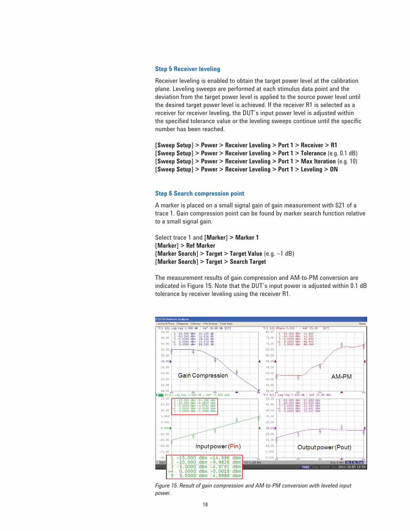
The measurement results of gain compression and AM-to-PM conversion are

indicated in Figure 15. Note that the DUT’s input power is adjusted within 0.1 dB

tolerance by receiver leveling using the receiver R1.

Figure 15. Result of gain compression and AM-to-PM conversion with leveled input

power.

19

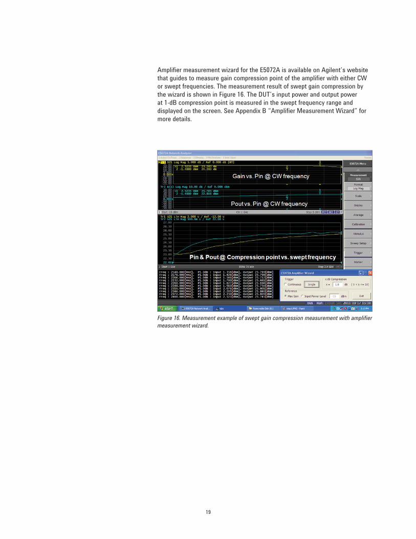
Amplifi er measurement wizard for the E5072A is available on Agilent’s website

that guides to measure gain compression point of the amplifi er with either CW

or swept frequencies. The measurement result of swept gain compression by

the wizard is shown in Figure 16. The DUT’s input power and output power

at 1-dB compression point is measured in the swept frequency range and

displayed on the screen. See Appendix B “Amplifi er Measurement Wizard” for

more details.

Figure 16. Measurement example of swept gain compression measurement with amplifi er

measurement wizard.

20

Figure 17. Harmonic distortion of amplifi ers.

Harmonic Distortion

Harmonic distortion is specifi ed to describe nonlinear behavior of amplifi er.

Harmonic level is defi ned as the difference in absolute power level between the

fundamental and the harmonics, expressed in dBc (dB relative to carrier) for a

specifi ed input or output power. (Figure 17)

Many applications require information regarding harmonics performance,

as excessive nonlinear distortion of the amplifi er causes adjacent channel

interference in communication systems. Traditionally, harmonics distortion

measurements have been performed with equipments such as a spectrum

analyzer and a signal generator. However, the E5072A offers frequency-offset

mode option (option 008) 1 which enables the source and receiver to sweep at

different frequencies for harmonics measurements. While the source is set to

the fundamental frequency, the receivers are tune to the desired harmonics.

By combining the frequency offset sweep and power level calibration such as

source power calibration and receiver calibration, fast and accurate harmon-

ics measurements can be performed with a single VNA. This can replace the

traditional method for measuring harmonic distortion using the combination of

a signal generator and spectrum analyzer and provide real-time CW or swept

frequency harmonics measurements.

The following describes necessary steps to measure harmonic distortion using

the E5072A. The power of the fundamental tone is measured in channel 1, while

the second and third harmonic is measured in channel 2 and 3 respectively. The

E5072A’s source from port 1 is set to the fundamental frequency for all channels

and the receiver B of port 2 is used as a receiver to measure the DUT’s output

power at fundamental and harmonic frequencies. An optional external attenua-

tor is needed on the port 2 to protect damage or compression of the receiver B.

This measurement process is described in the following steps:


Step 2 Power calibration & receiver calibration in harmonic frequency range

Step 3 Power calibration in fundamental frequency range

Step 4 Perform harmonic measurements

In Step 2, receiver calibration with the power-calibrated source is performed for

absolute measurements in all channels. The frequency range for this calibration

is set in harmonic frequency range. And then, power calibration is performed for

the source in fundamental frequency range in Step 3 to get accurate power level

at the DUT’s input for harmonics measurements.

fo 3fo2fo . . .fo

Ou

tpu

t pow

er (

dB

m)

Delta (dBc)

fo 3fo2fo

1. See the E5072A configuration guide, part

number 5990-8001EN.


pdf/5990-8001EN.pdf) for more detail.

21


Stimulus parameters such as frequency, IFBW or NOP should be entered for

channel 1, 2 and 3.

(1) Setup channel 1 for fundamental

Stimulus parameters such as frequency, IFBW or source power level for

fundamental signal are entered in channel 1. The absolute measurement

using the receiver B is selected for a measurement trace. Three channels

are allocated on the screen.

[Meas] > Absolute > B (1)

[Start] (e.g. 1.2 GHz)

[Stop] (e.g. 1.5 GHz)

[Avg] > IF Bandwidth (e.g. 1 kHz)

[Sweep Setup] > Points (e.g. 51)

[Sweep Setup] > Power > Power (e.g. 0 dBm)

[Display] > Allocate Channel (x3)

(2) Setup channel 2 for second harmonic

Channel 2 is selected and stimulus parameters are entered as the same as

channel 1. In addition, Frequency-offset mode (FOM) is enabled and the

source and receiver frequency is tuned at second harmonic frequency

range (e.g. 2.4 to 3 GHz).

[Sweep Setup] > Frequency Offset > Port 1 > Multiplier (2)


[Sweep Setup] > Frequency Offset > Frequency Offset (On)

(3) Setup channel 3 for third harmonic

Channel 3 is selected and stimulus parameters are entered as the same as

channel 1 or 2. FOM is enabled and the source and receiver frequency is

tuned at third harmonic frequency range (e.g. 3.6 to 4.5 GHz).



[Sweep Setup] > Frequency Offset > Frequency Offset (On)

22

Step 2 Power calibration & receiver calibration in harmonic frequency range

(1) Perform power calibration

Power calibration is necessary prior to receiver calibration in order to

accurately characterize the E5072A’s receivers for absolute measurements.

A power sensor is connected to the E5072A’s port 1 and power calibration

is performed at: fundamental frequency (f1) in channel 1, second harmonic

frequency (f2) in channel 2 and third harmonic frequency (f3) in channel 3

respectively. (Figure 18)




Figure 18. Confi guration of power calibration for harmonics frequency range.

Port 1 Port 2

Power Sensor

(i.e. Agilent U2000 Series)

Connected to the E5072A

f1

f2

f3

Ch 1

Ch 2

Ch 3

23

(2) Perform receiver calibration

After connecting a thru between the port 1 and port 2, receiver calibration

is performed for absolute measurements using the receiver B for all

channels. The receiver B is calibrated in the frequency range of the

fundamental in channel 1, second harmonic in channel 2, and third

harmonic in channel 3 respectively. (Figure 19)

[Cal] > Receiver Calibration > Select Receiver > B


Figure 19. Confi guration of receiver calibration for harmonics frequency range.

Port 1 Port 2

B

Attenuator

(optional)

Thru

Ch 1: f1

Ch 2: f2

Ch 3: f3

Ch 1: f1

Ch 2: f2

Ch 3: f3

24

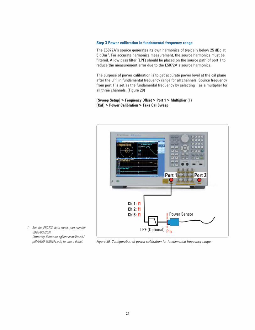
Figure 20. Confi guration of power calibration for fundamental frequency range.

Port 1 Port 2

Power Sensor

LPF (Optional)

Ch 1: f1

Ch 2: f1

Ch 3: f1

Pin

Step 3 Power calibration in fundamental frequency range

The E5072A’s source generates its own harmonics of typically below 25 dBc at

5 dBm 1. For accurate harmonics measurement, the source harmonics must be

fi ltered. A low pass fi lter (LPF) should be placed on the source path of port 1 to

reduce the measurement error due to the E5072A’s source harmonics.

The purpose of power calibration is to get accurate power level at the cal plane

after the LPF in fundamental frequency range for all channels. Source frequency

from port 1 is set as the fundamental frequency by selecting 1 as a multiplier for

all three channels. (Figure 20)



1. See the E5072A data sheet, part number

5990-8002EN.


pdf/5990-8002EN.pdf) for more detail.

25

Step 4 Perform harmonic measurements

The DUT is connected and harmonics measurements are performed for all three

channels of the E5072A (Figure 21). The harmonics measurement example of an

amplifi er with swept frequency input is indicated in Figure 22. The fundamental

power is monitored with the absolute measurement in channel 1, while second

and harmonics are monitored in channel 2 and 3.

Figure 21. Confi guration of harmonic measurements with the E5072A.

Figure 22. Measurement result of swept harmonic measurement.

Port 1 Port 2

B

Attenuator

(optional)

Ch 1: f1

Ch 2: f2

Ch 3: f3

LPF (Optional)

Ch 1: f1

Ch 2: f1

Ch 3: f1

Pin

DUT

26

Figure 23. Measurement example of swept harmonic measurement with amplifi er

measurement wizard.

Amplifi er measurement wizard for the E5072A guides you through swept-

frequency harmonics measurements. The measurement example of swept

frequency harmonics by the wizard is shown in Figure 23. The power level of

fundamental and up to 5th harmonics (in dBm), and harmonics relative to carrier

(in dBc) can be monitored by with the utility wizard. See Appendix B “Amplifi er

Measurement Wizard” for more details.

27

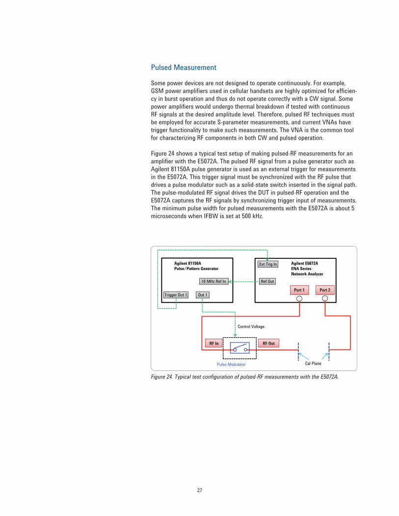
Pulsed Measurement

Some power devices are not designed to operate continuously. For example,

GSM power amplifi ers used in cellular handsets are highly optimized for effi cien-

cy in burst operation and thus do not operate correctly with a CW signal. Some

power amplifi ers would undergo thermal breakdown if tested with continuous

RF signals at the desired amplitude level. Therefore, pulsed RF techniques must

be employed for accurate S-parameter measurements, and current VNAs have

trigger functionality to make such measurements. The VNA is the common tool

for characterizing RF components in both CW and pulsed operation.

Figure 24 shows a typical test setup of making pulsed-RF measurements for an

amplifi er with the E5072A. The pulsed RF signal from a pulse generator such as

Agilent 81150A pulse generator is used as an external trigger for measurements

in the E5072A. This trigger signal must be synchronized with the RF pulse that

drives a pulse modulator such as a solid-state switch inserted in the signal path.

The pulse-modulated RF signal drives the DUT in pulsed-RF operation and the

E5072A captures the RF signals by synchronizing trigger input of measurements.

The minimum pulse width for pulsed measurements with the E5072A is about 5

microseconds when IFBW is set at 500 kHz.

Figure 24. Typical test confi guration of pulsed-RF measurements with the E5072A.

Agilent 81150A

Pulse/Pattern Generator Agilent E5072A

ENA Series

Network Analyzer

10 MHz Ref In Ref Out

Port 1 Port 2Trigger Out 1 Out 1

Cal Plane

RF In RF Out

Ext Trig In

Pulse Modulator

Control Voltage

28

Figure 25. Timing chart of pulsed-RF measurements with the E5072A.

The typical timing chart for pulsed measurements is shown in Figure 25. Sam-

pling or data acquisition in the E5072A must take place during the RF pulse, and

this is achieved by externally triggering the analyzers to measure the appropriate

points in time. It is important to remember that there is some latency or delay

between the external pulse trigger and when the sampling actually starts in the

E5072A (indicated as “Td” in Figure 25). This means the E5072A must be trig-

gered before the RF pulse is applied from a pulse generator. Note that there is

some inherent settling time on the E5072A before the setup of parameters such

as sweep frequency, IFBW, or power level. The typical delay time of the E5072A

is about 12.3 microseconds.

Delay

RF On

Period

Duty cycle (%)

Td Ts Ta Td

Pulse Width

RF On RF On RF On

81150A Trigger OUT 1

81150A Out 1 (Pulsed RF Signal)

E5072A Ex. Trigger Input

E5072A Data Acquisition

E5072A Performance:

Td = 12.3 ± 0.1 us (typ.)

Ts = 5 us (min. @ IFBW 500 kHz)Ta = 10 us (min.)

29

Figure 26. Test confi guration of pulsed-RF measurements using receiver leveling of the

E5072A.

Port 1 Port 2R1

B

Attenuator

(optional)

Pulse

modulator

CouplerPin Pout

DUT

As many devices under pulsed condition are active devices and the characteris-

tics including compression and distortion are typically sensitive to input power

level. Inaccurate stimulus power may introduce considerable measurement er-

rors and it is critical to employ the appropriate techniques for accurately leveling

the stimulus power. Power level calibration techniques such as receiver leveling

are recommended for pulsed measurements with the E5072A.

The following describes the necessary steps for the pulsed RF measurement

using the E5072A. Input and output power of the DUT in pulsed operation are

monitored by absolute measurements with the E5072A. The output signal of

the pulse modulator is measured by the receiver R1, and temperature drift of

the modulator is eliminated by the receiver leveling with the E5072A to get

accurate power level at the DUT’s input. The DUT’s output power is monitored

by absolute measurements using the receiver B. The test confi guration of the

measurement with the E5072A is shown in Figure 26.

30

Step 1 Setup of a pulse generator

Pulse width, pulse period or signal levels of pulse signals are setup by a pulse

generator such as Agilent 81150A pulse generator. The trigger delay can be setup

by a pulse generator with accurate resolution. The pulsed signals are supplied to a

pulse modulator in the signal path and the external trigger input of the E5072A.


Stimulus parameters such as frequency, IFBW or NOP should be entered on

the E5072A before calibration and measurements. Note that IFBW should be

wide enough for data acquisition when narrow pulse width is required for the

measurement. The minimum pulse width for the E5072A is about 5 microsec-

onds when 500 kHz is selected for IFBW.

[Avg] > IF Bandwidth (e.g. 500 kHz)


Power calibration with a power sensor connected at the calibration plane is

performed to get accurate power level at the DUT’s input by compensating the

loss of the pulse modulator or coupler in the signal path. Note that duty cycle

of a pulse generator should be set at 100% when the average power sensor is

used for power calibration.

[Cal] > Power Calibration > Select Port (1)




Step 4 Receiver Calibration

Receiver calibration is necessary for accurate absolute measurements. A thru is

connected between the port 1 and port 2 and receiver calibration for the receiver

R1 and receiver B is performed. When an absolute measurement of each

receiver is selected as a measurement trace, input or output power level of the

DUT is displayed after receiver calibration.





Step 5 Calibration

For S-parameter calibration in pulsed condition, external trigger input must be

selected as a trigger source for the calibration. To minimize the variation of the

delay time between trigger input and data acquisition for accurate timing setup,

it is recommended that the low-latency external trigger mode be turned on with

the [Low Latency] soft key.

[Trigger] > Trigger Source > External

[Trigger] > Trigger Event > On Point

[Trigger] > Low Latency (On)

31

Calibration using mechanical cal kits is required for synchronized calibration

measurements with external trigger input. An appropriate calibration technique

under [Cal] hard key is selected and calibration is performed with pulsed-RF

signals. Note that duty cycle of pulsed signals from the pulse generator should

be set before calibration measurements to apply pulsed RF signals to a pulse

modulator and the E5072A.


To remove the temperature drift of a pulse modulator, receiver leveling using the

receiver measurement is useful. The source power from the E5072A is adjusted

to get accurate targeted power level at the DUT’s input.

[Sweep Setup] > Power > Receiver Leveling > Port 1 > Receiver > R1



[Sweep Setup] > Power > Receiver Leveling > Port 1 > Leveling (ON)

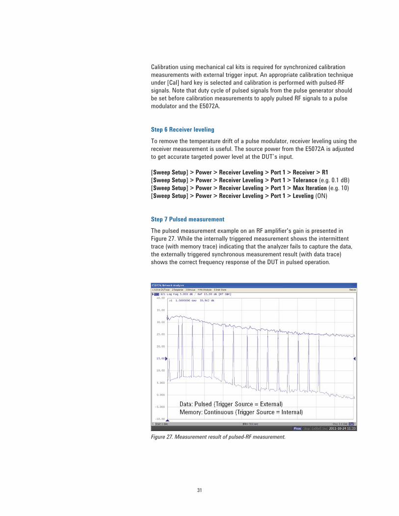
Step 7 Pulsed measurement

The pulsed measurement example on an RF amplifi er's gain is presented in

Figure 27. While the internally triggered measurement shows the intermittent

trace (with memory trace) indicating that the analyzer fails to capture the data,

the externally triggered synchronous measurement result (with data trace)

shows the correct frequency response of the DUT in pulsed operation.

Figure 27. Measurement result of pulsed-RF measurement.

32

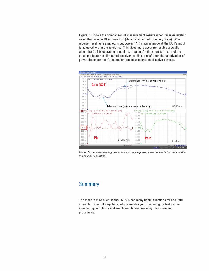
Figure 28 shows the comparison of measurement results when receiver leveling

using the receiver R1 is turned on (data trace) and off (memory trace). When

receiver leveling is enabled, input power (Pin) in pulse mode at the DUT’s input

is adjusted within the tolerance. This gives more accurate result especially

when the DUT is operating in nonlinear region. As the short-term drift of the

pulse modulator is eliminated, receiver leveling is useful for characterization of

power-dependent performance or nonlinear operation of active devices.

Figure 28. Receiver leveling makes more accurate pulsed measurements for the amplifi er

in nonlinear operation.

The modern VNA such as the E5072A has many useful functions for accurate

characterization of amplifi ers, which enables you to reconfi gure test system

eliminating complexity and simplifying time-consuming measurement

procedures.

Summary

33

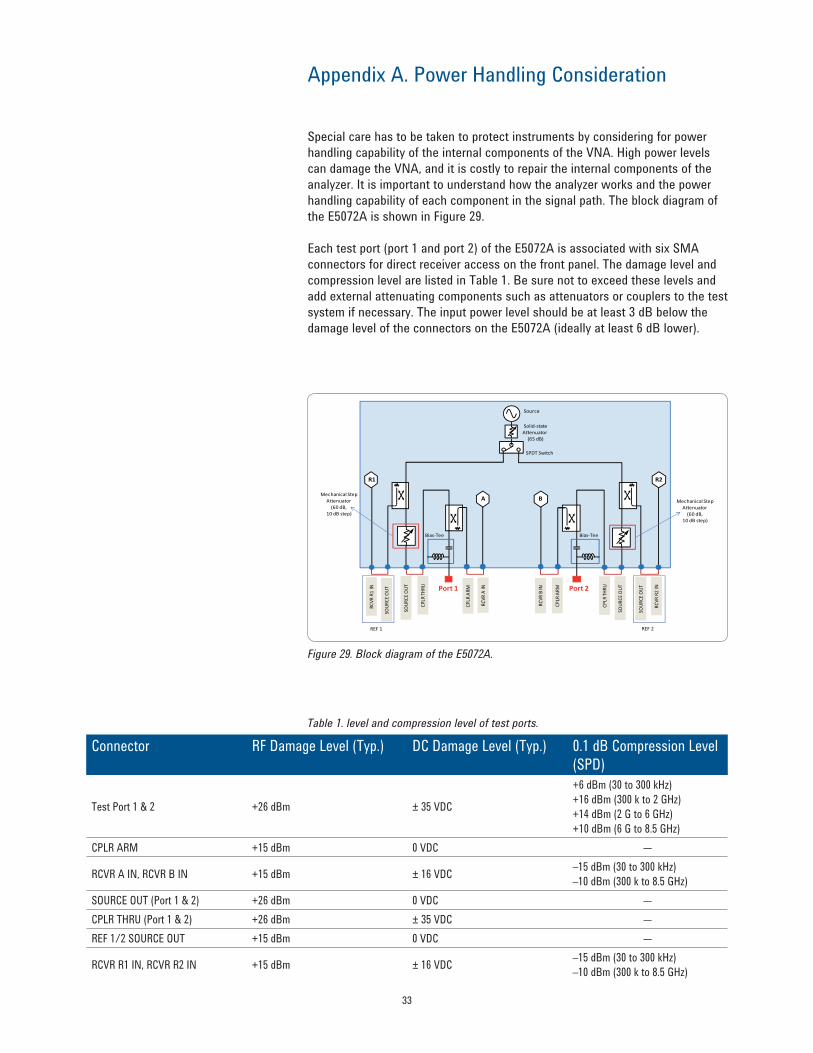
Special care has to be taken to protect instruments by considering for power

handling capability of the internal components of the VNA. High power levels

can damage the VNA, and it is costly to repair the internal components of the

analyzer. It is important to understand how the analyzer works and the power

handling capability of each component in the signal path. The block diagram of

the E5072A is shown in Figure 29.

Each test port (port 1 and port 2) of the E5072A is associated with six SMA

connectors for direct receiver access on the front panel. The damage level and

compression level are listed in Table 1. Be sure not to exceed these levels and

add external attenuating components such as attenuators or couplers to the test

system if necessary. The input power level should be at least 3 dB below the

damage level of the connectors on the E5072A (ideally at least 6 dB lower).

Appendix A. Power Handling Consideration

Connector RF Damage Level (Typ.) DC Damage Level (Typ.) 0.1 dB Compression Level (SPD)

Test Port 1 & 2 +26 dBm ± 35 VDC

+6 dBm (30 to 300 kHz)

+16 dBm (300 k to 2 GHz)

+14 dBm (2 G to 6 GHz)

+10 dBm (6 G to 8.5 GHz)

CPLR ARM +15 dBm 0 VDC ―

RCVR A IN, RCVR B IN +15 dBm ± 16 VDC–15 dBm (30 to 300 kHz)

–10 dBm (300 k to 8.5 GHz)

SOURCE OUT (Port 1 & 2) +26 dBm 0 VDC ―

CPLR THRU (Port 1 & 2) +26 dBm ± 35 VDC ―

REF 1 /2 SOURCE OUT +15 dBm 0 VDC ―

RCVR R1 IN, RCVR R2 IN +15 dBm ± 16 VDC–15 dBm (30 to 300 kHz)

–10 dBm (300 k to 8.5 GHz)

Figure 29. Block diagram of the E5072A.

R1

A

R2

B

Port 1 Port 2

RCVR

R1

IN

SOU

RCE

OU

T

CPLR

TH

RU

SOU

RCE

OU

T

RCVR

A IN

CPLR

ARM

RCVR

B IN

CPLR

ARM

CPLR

TH

RU

SOU

RCE

OU

T

RCVR

R2

IN

SOU

RCE

OU

T

Source

SPDT Switch

Solid-stateA�enuator

(65 dB)

Mechanical Step A�enuator

(60 dB, 10 dB step)

Bias-Tee Bias-Tee

Mechanical Step A�enuator

(60 dB, 10 dB step)

REF 1 REF 2

Table 1. level and compression level of test ports.

34

Figure 30. Amplifi er measurement wizard for the E5072A.

The ENA Series includes Microsoft VBA Macro programming capability, a

time-saving tool for test automation. You can customize your interface easily

to optimize the operating environment at no additional cost and you can also

add automation processes. Many VBA sample programs for the ENA series are

available on Agilent’s website (www.agilent.com/find/enavba) to help you

create your own program library for your applications.

Amplifi er measurement wizard for the E5072A is provided for basic amplifi er

measurements. (Figure 30) This utility program supports the following measure-

ments of amplifi ers with the E5072A:

S-parameters / K-factor

Swept-frequency harmonic distortion

Gain compression and AM-to-PM Conversion (CW)

Swept-frequency gain compression

It guides you through measurement procedures to setup parameters and

perform necessary calibration for measurements, so that you can minimize the

time spent on measurement setup. High-power amplifi er measurements with

the E5072A using an external booster amplifi er are also supported by the wizard.

Appendix B. Amplifi er Measurement Wizard

35

The comparison of the Agilent E5071C and E5072A ENA Series Network

Analyzer is shown in table 2. The E5072A is a more suited solution for RF

amplifi er characterization.

Appendix C. Comparison with E5071C

Features/ Functions E5071C 2-port RF Options(opt.24x, 26x, 28x)

E5072A

Confi gurable test set

(Direct receiver access)No Yes (standard)

Uncoupled power (with source attenuators) No Yes

Max output power +10 dBm (up to 5 GHz)+16 dBm (spec, up to 3 GHz)

+20 dBm (SPD 1, 300 k to 1 GHz)

Power calibration YesYes (More accurate with tolerance and max

iteration)

Receiver calibration Yes Yes (with four independent receivers)

Receiver Leveling No Yes

Harmonic distortion Yes (with FOM option) Yes (with FOM option)

Pulsed-RF Yes (wide pulse width) Yes (wide pulse width)

Amplifi er measurement wizard YesYes (High-power measurement is also

supported.)

Equation Editor Yes Yes

References

E5072A Configuration Guide, part number 5990-8001EN

http://cp.literature.agilent.com/litweb/pdf/5990-8001EN.pdf

E5072A Data Sheet, part number 5990-8002EN


E5072A Quick Fact Sheet, part number 5990-8003EN


E5072A Technical Overview, part number 5990-8004EN


High-power Measurement Using the E5072A, part number 5990-8005EN


7 Reasons to update from the 8753 to the ENA, part number 5989-0206EN


ENA series web page: http://www.agilent.com/find/ena

E5072A web page: http://www.agilent.com/find/e5072a

Agilent 81150A and 81160A Pulse Function Arbitrary Noise Generators Data Sheet


Table 2. Comparison with the E5071C ENA series network analyzer.

1. The value is supplemental performance data or SPD that is most likely occur. Not guaranteed by

the product warranty.

www.agilent.com

www.agilent.com/quality

Agilent Email Updates

www.agilent.com/find/emailupdates

Get the latest information on the

products and applications you select.

www.lxistandard.org

LAN eXtensions for Instruments puts

the power of Ethernet and the Web

inside your test systems. Agilent is a

founding member of the LXI consortium.

Agilent Channel Partners

www.agilent.com/find/channelpartners

Get the best of both worlds: Agilent’s

measurement expertise and product

breadth, combined with channel

partner convenience.

Agilent Advantage Services is committed

to your success throughout your equip-

ment’s lifetime. To keep you competitive,

we continually invest in tools and

processes that speed up calibration and

repair and reduce your cost of ownership.

You can also use Infoline Web Services

to manage equipment and services more

effectively. By sharing our measurement

and service expertise, we help you create

the products that change our world.

www.agilent.com/find/advantageservices

For more information on Agilent Technologies’ products, applications or services, please contact your local Agilent

office. The complete list is available at:

www.agilent.com/fi nd/contactus

AmericasCanada (877) 894 4414 Brazil (11) 4197 3600Mexico 01800 5064 800 United States (800) 829 4444

Asia Pacifi cAustralia 1 800 629 485China 800 810 0189Hong Kong 800 938 693India 1 800 112 929Japan 0120 (421) 345Korea 080 769 0800Malaysia 1 800 888 848Singapore 1 800 375 8100Taiwan 0800 047 866Other AP Countries (65) 375 8100

Europe & Middle EastBelgium 32 (0) 2 404 93 40 Denmark 45 45 80 12 15Finland 358 (0) 10 855 2100France 0825 010 700* *0.125 €/minute

Germany 49 (0) 7031 464 6333 Ireland 1890 924 204Israel 972-3-9288-504/544Italy 39 02 92 60 8484Netherlands 31 (0) 20 547 2111Spain 34 (91) 631 3300Sweden 0200-88 22 55United Kingdom 44 (0) 118 927 6201

For other unlisted countries: www.agilent.com/fi nd/contactusRevised: January 6, 2012

Product specifications and descriptions in this document subject to change without notice.

© Agilent Technologies, Inc. 2012Published in USA, March 22 20125990-9974EN

Basics of RF Ampliﬁ er Measurements with the E5072A ENA ... · Basics of RF Ampliﬁ er...

Documents

Transcript of Basics of RF Ampliﬁ er Measurements with the E5072A ENA ... · Basics of RF Ampliﬁ er...