Basic Statistics

Inferences About Two Population Means

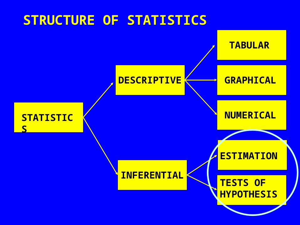
STRUCTURE OF STATISTICS

STATISTICS

DESCRIPTIVE

INFERENTIAL

TABULAR

GRAPHICAL

NUMERICAL

ESTIMATION

TESTS OF HYPOTHESIS

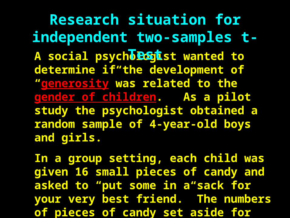
A social psychologist wanted to determine if the development of “generosity”was related to the gender of children. As a pilot study the psychologist obtained a random sample of 4-year-old boys and girls.

In a group setting, each child was given 16 small pieces of candy and asked to “put some in a sack for your very best friend.” The numbers of pieces of candy set aside for friend by 10 girls and 10 boys are shown below:

Research situation for independent two-samples t-Test

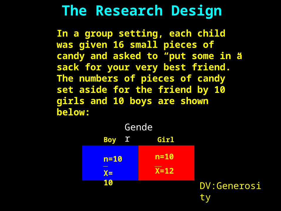
The Research Design

In a group setting, each child was given 16 small pieces of candy and asked to “put some in a sack for your very best friend.” The numbers of pieces of candy set aside for the friend by 10 girls and 10 boys are shown below:

GenderBoy Girl

n=10

X= 10

n=10

X=12

DV:Generosity

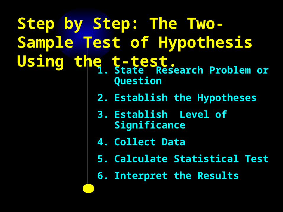
Step by Step: The Two-Sample Test of Hypothesis Using the t-test.

1. State Research Problem or Question

2. Establish the Hypotheses

3. Establish Level of Significance

4. Collect Data

5. Calculate Statistical Test

6. Interpret the Results

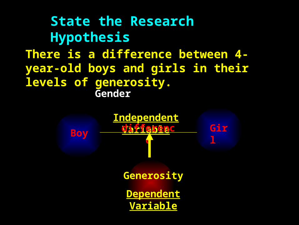
State the Research Hypothesis

There is a difference between 4-year-old boys and girls in their levels of generosity.

Boy Girl

Generosity

Dependent Variable

Gender Independent Variable

difference

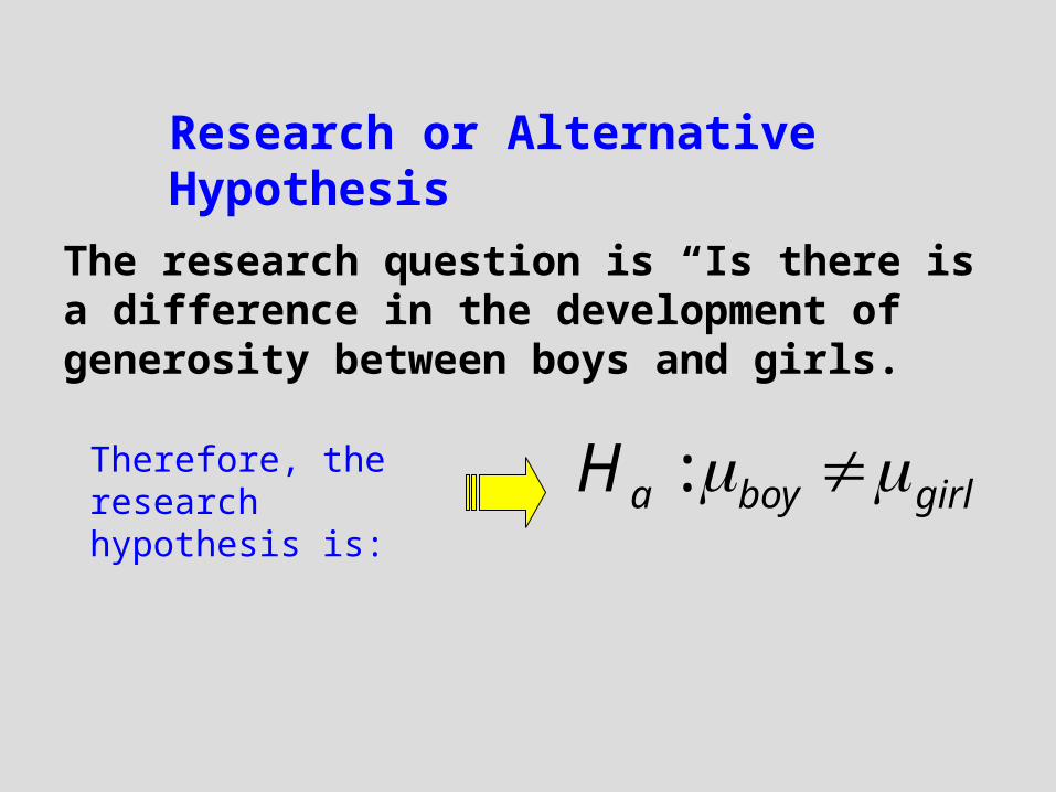
The research question is “Is there is a difference in the development of generosity between boys and girls.

Research or Alternative Hypothesis

Therefore, the research hypothesis is: girlboyaH :

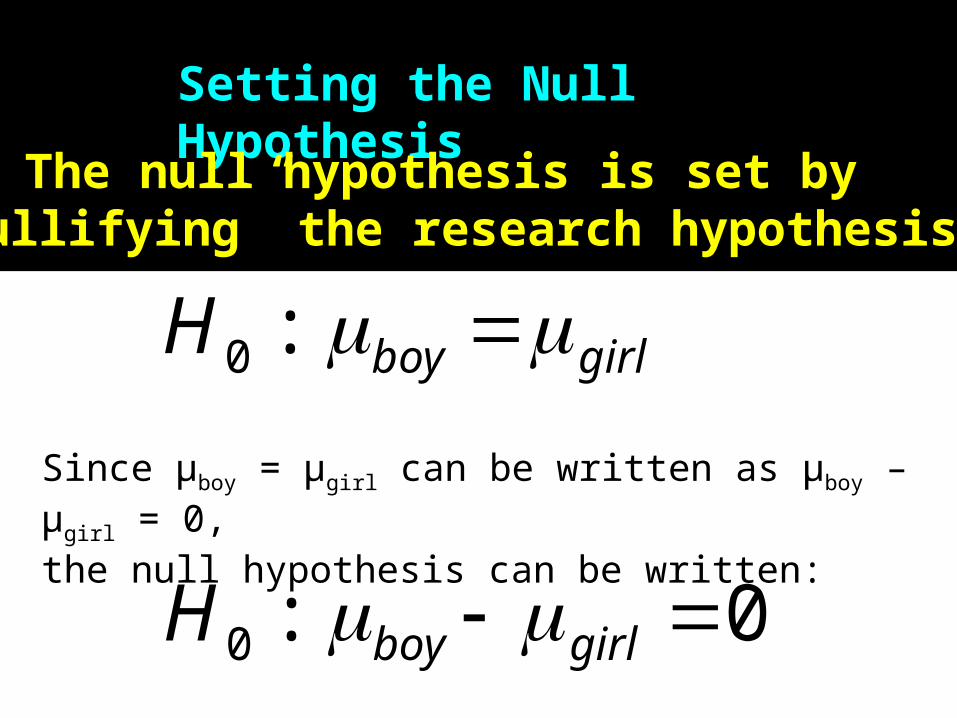
Setting the Null Hypothesis

The null hypothesis is set by “nullifying” the research hypothesis.

girlboyH :0

Since μboy = μgirl can be written as μboy – μgirl = 0, the null hypothesis can be written:

0:0 girlboyH

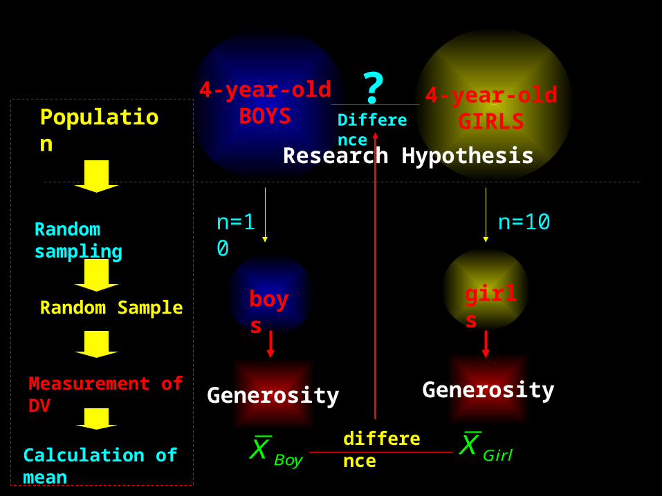
Generosity

4-year-old BOYS GIRL

boys girls

n=10 n=10

Population

Random sampling

Measurement of DV

4-year-old GIRLS

Random Sample

Generosity

BoyX GirlXCalculation of meandifference

?Difference

Research Hypothesis

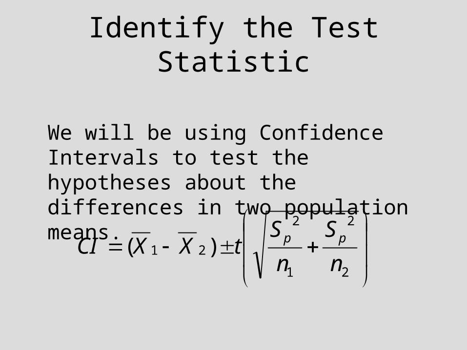
Identify the Test Statistic

We will be using Confidence Intervals to test the hypotheses about the differences in two population means.

2

2

1

2

21 )(n

S

n

StXXCI pp

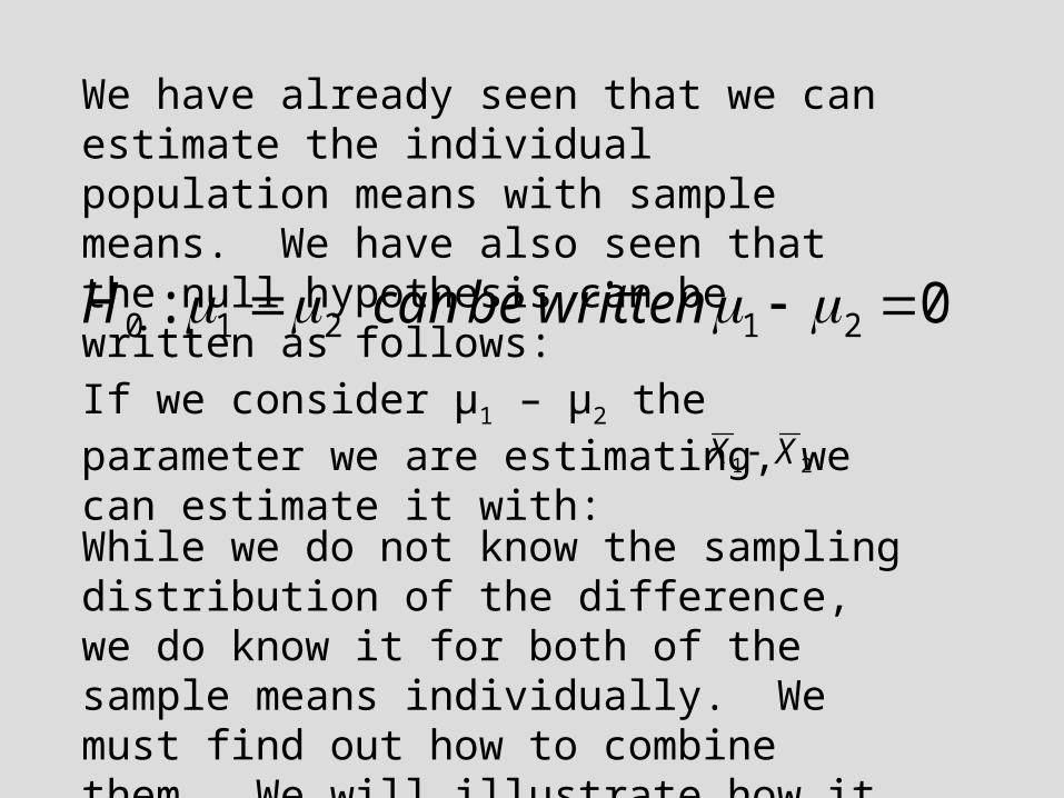
We have already seen that we can estimate the individual population means with sample means. We have also seen that the null hypothesis can be written as follows:

0: 21210 writtenbecanH

If we consider μ1 – μ2 the parameter we are estimating, we can estimate it with: 21 XX

While we do not know the sampling distribution of the difference, we do know it for both of the sample means individually. We must find out how to combine them. We will illustrate how it might be done with a simple example.

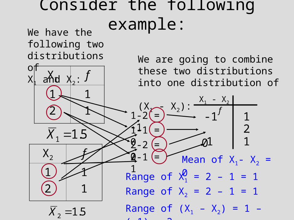
Consider the following example:

X2 f

1

2

1

1

X1 f

1

2

1

1

We have the following two distributions of X1 and X2: We are going to combine these two

distributions into one distribution of

(X1 - X2):

1-2 = -1

5.11 X

5.12 X

-1

X1 - X2 f

11-1 = 0 0 12-2 = 0 1

2

2-1 = 1

1

Range of X1 = 2 – 1 = 1

Range of X2 = 2 – 1 = 1

Range of (X1 – X2) = 1 – (-1) = 2

Mean of X1- X2 = 0

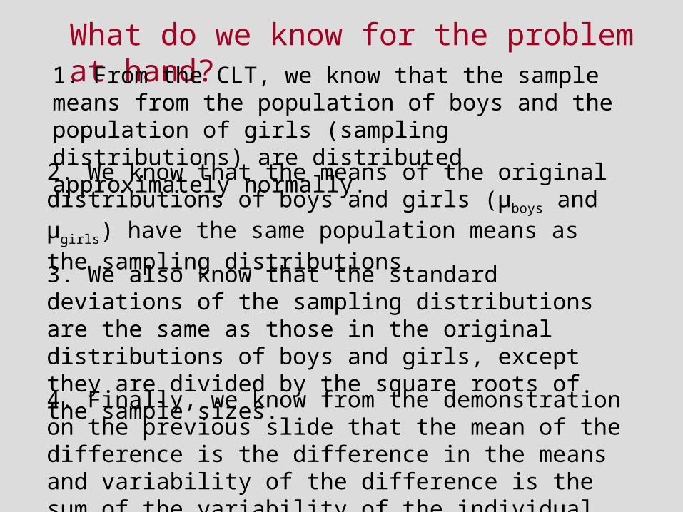
What do we know for the problem at hand?1. From the CLT, we know that the sample means from the population of boys and the population of girls (sampling distributions) are distributed approximately normally.

2. We know that the means of the original distributions of boys and girls (μboys and μgirls) have the same population means as the sampling distributions.

3. We also know that the standard deviations of the sampling distributions are the same as those in the original distributions of boys and girls, except they are divided by the square roots of the sample sizes.

4. Finally, we know from the demonstration on the previous slide that the mean of the difference is the difference in the means and variability of the difference is the sum of the variability of the individual distributions.

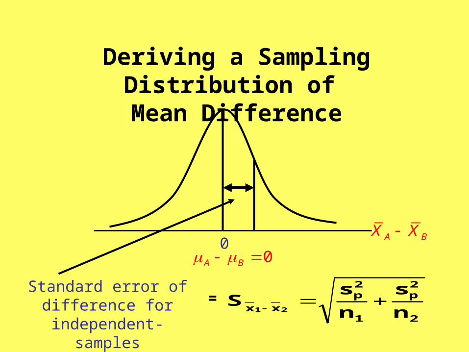
0

Standard error of difference for independent-

samples

A BX X

Deriving a Sampling Distribution of Mean Difference

0A B

2

2p

1

2p

xx n

s

n

sS

21

=

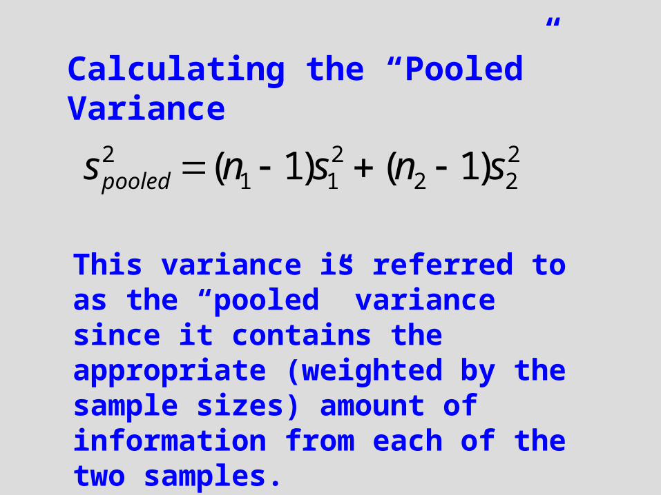
Calculating the “Pooled” Variance

This variance is referred to as the “pooled” variance since it contains the appropriate (weighted by the sample sizes) amount of information from each of the two samples.

222

211

2 )1()1( snsnspooled

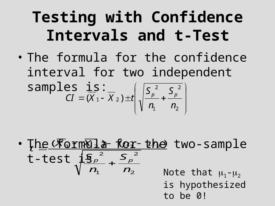
Testing with Confidence Intervals and t-Test

• The formula for the confidence interval for two independent samples is:

• The formula for the two-sample t-test is

2

2

1

2

21 )(n

S

n

StXXCI pp

2

2

1

2

2121 )()(

n

S

n

S

XXt

pp

Note that 1-2 is hypothesized to be 0!

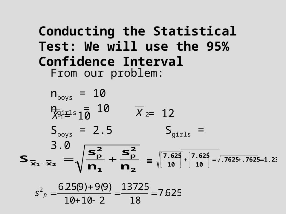
Conducting the Statistical Test: We will use the 95% Confidence Interval

From our problem:

nboys = 10 ngirls = 10

1X 2X = 12 = 10Sboys = 2.5 Sgirls = 3.0

2

2p

1

2p

xx n

s

n

sS

21 =

625.718

25.137

21010

)9(9)9(25.62

ps

1.23.7625.762510

7.625

10

7.625

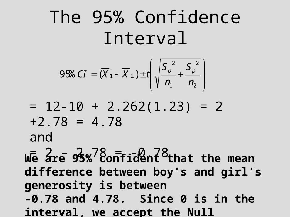
The 95% Confidence Interval

2

2

1

2

21 )(%95n

S

n

StXXCI pp

= 12-10 + 2.262(1.23) = 2 +2.78 = 4.78 and = 2 – 2.78 = -0.78

We are 95% confident that the mean difference between boy’s and girl’s generosity is between –0.78 and 4.78. Since 0 is in the interval, we accept the Null Hypothesis of no difference in generosity.

0

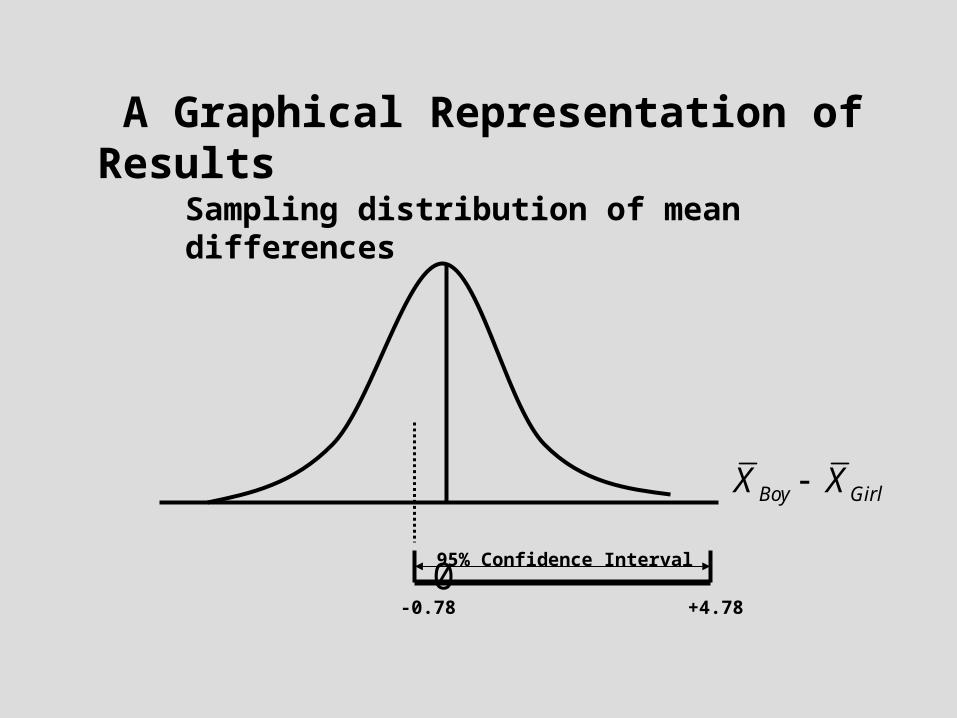
A Graphical Representation of Results

Sampling distribution of mean differences

Boy GirlX X

-0.78 +4.78

95% Confidence Interval

The “Dependent” Samples t-test

The previous example assumed independent random sampling. What if the two samples are dependent on each other?

An Example

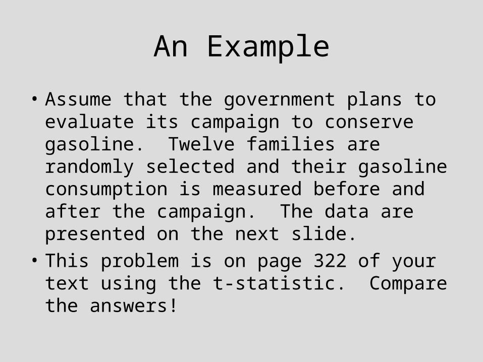
• Assume that the government plans to evaluate its campaign to conserve gasoline. Twelve families are randomly selected and their gasoline consumption is measured before and after the campaign. The data are presented on the next slide.

• This problem is on page 322 of your text using the t-statistic. Compare the answers!

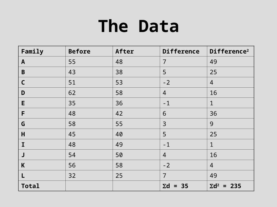
The DataFamily Before After Difference Difference2

A 55 48 7 49

B 43 38 5 25

C 51 53 -2 4

D 62 58 4 16

E 35 36 -1 1

F 48 42 6 36

G 58 55 3 9

H 45 40 5 25

I 48 49 -1 1

J 54 50 4 16

K 56 58 -2 4

L 32 25 7 49

Total d = 35 d2 = 235

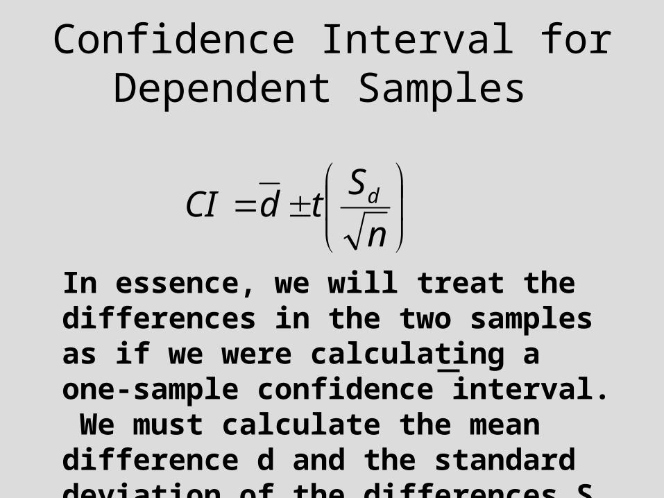
In essence, we will treat the differences in the two samples as if we were calculating a one-sample confidence interval. We must calculate the mean difference d and the standard deviation of the differences Sd

Confidence Interval for Dependent Samples

n

StdCI d

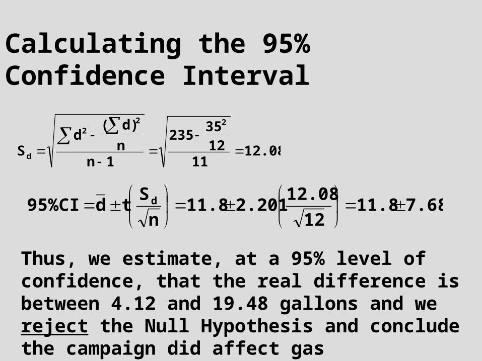
Calculating the 95% Confidence Interval

12.0811

1235

235

1nn

d)(d

S

222

d

7.6811.812

12.082.20111.8

n

Std95%CI d

Thus, we estimate, at a 95% level of confidence, that the real difference is between 4.12 and 19.48 gallons and we reject the Null Hypothesis and conclude the campaign did affect gas consumption. (see page 324)

Summary of Two Sample Tests

• We can use confidence intervals to test an hypothesis about the difference in two independent samples.

• We can also use confidence intervals to test an hypothesis about the difference in two dependent samples.

• The conclusions reached using confidence intervals are exactly the same as using the t-statistic.