Barbara M. Fraumeni Muskie School of Public Service, USM, Portland, ME & the National Bureau of...
27
Barbara M. Fraumeni ie School of Public Service, USM, Portland, the National Bureau of Economic Research, U ference of European Statisticians, UNECE/OECD/Euros Task Force on Measuring Sustainable Development Geneva, Switzerland September 24, 2009 Construction of Human Capital Accounts in the Measurement of Sustainable Development uskie School of Public Service Ph.D. Program in Public Policy
-
Upload
candace-mccarthy -
Category
Documents
-
view
214 -
download
1
Transcript of Barbara M. Fraumeni Muskie School of Public Service, USM, Portland, ME & the National Bureau of...

Barbara M. FraumeniMuskie School of Public Service, USM, Portland, ME
& the National Bureau of Economic Research, USA
Conference of European Statisticians, UNECE/OECD/EurostatTask Force on Measuring Sustainable Development
Geneva, Switzerland September 24, 2009
Construction of Human Capital Accountsin the
Measurement of Sustainable Development
Muskie School of Public Service Ph.D. Program in Public Policy

2
Sustainable development as development that meets
“…the needs of the present without compromising the ability of future
generations to meet their own needs”
World Commissionon Environment & Development, 1987
Muskie School of Public Service Ph.D. Program in Public Policy

3
Importance of Human Capital
• Role in satisfying the present and future needs of humankind
• Not just the impact of humans on natural resources and the environment
Muskie School of Public Service Ph.D. Program in Public Policy

4
Context for Constructing Human Capital Accounts
• OECD consortium
• Jorgenson-Fraumeni human capital accounts have been constructed for Australia, Canada, China, New Zealand, Norway, Sweden and the United States
• “New” countries using J-F methodology will facilitate cross-country comparisons
Muskie School of Public Service Ph.D. Program in Public Policy

5
Recommend that countries initially
estimate only market lifetime income
Muskie School of Public Service Ph.D. Program in Public Policy

6
J-F Approach
Human capital is measured as lifetime income, e.g., present and
future income
Muskie School of Public Service Ph.D. Program in Public Policy

7
J-F Approach
• All of the data listed below is needed for even a market only approach
• By individual years of age & level of education (highest level attained or enrollment)– Population– Enrollment– Labor compensation– Survival rates (by sex and age only)
Muskie School of Public Service Ph.D. Program in Public Policy

8
J-F (1992) “The Output of the Labor Income
• From contemporary information and data sets, assess the probabilities that persons will go to school, perform market work, and live
• Future wage rates (labor incomes) are assumed to increase at a specified rate
• Future labor incomes are discounted
Muskie School of Public Service Ph.D. Program in Public Policy

9
J-F (1992) “The Output of the Education Sector”
Methodology
• Backwards recursive
• Estimates dependent upon those older in the calendar year, e.g., relative future wage rates (labor incomes) come from contemporary relationships
• Stages dictated by data availability
Muskie School of Public Service Ph.D. Program in Public Policy

10
J-F (1992) “The Output of the Education Sector”
Five Stages
• Stage 1: No school or work, ages 0-4
• Stage 2: School, but no work, ages 5-15
• Stage 3: School and work, ages 16-34
• Stage 4: Work only, ages 35-74
• Stage 5: Retirement, zero income, ages 75 or older
Muskie School of Public Service Ph.D. Program in Public Policy
11
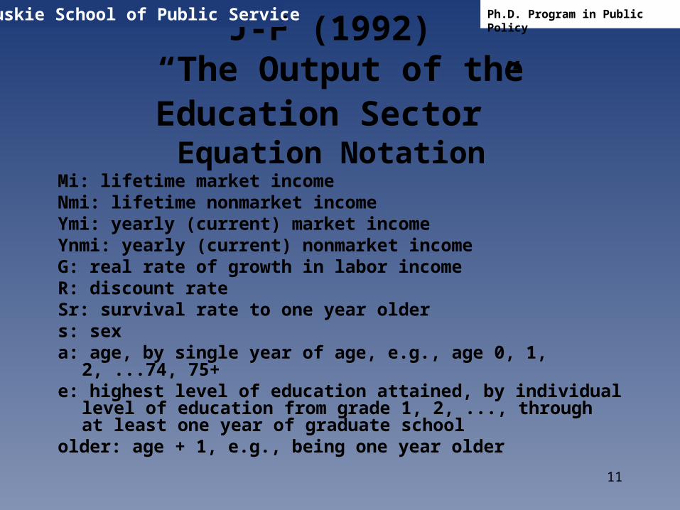
J-F (1992) “The Output of the Education Sector”
Equation Notation
Mi: lifetime market income Nmi: lifetime nonmarket incomeYmi: yearly (current) market incomeYnmi: yearly (current) nonmarket incomeG: real rate of growth in labor incomeR: discount rateSr: survival rate to one year olders: sexa: age, by single year of age, e.g., age 0, 1, 2, ...74, 75+e: highest level of education attained, by individual level of education
from grade 1, 2, ..., through at least one year of graduate schoololder: age + 1, e.g., being one year older
Muskie School of Public Service Ph.D. Program in Public Policy

12
J-F (1992) “The Output of the Education Sector”
Equations for Ages 35-74
mi(s,a,E) = ymi(s,a,e) + sr(s,older) * mi(s,older,e) * (1+g)/(1+r)
nmi(s,a,e) = ynmi(s,a,e) + sr(s,older) * nmi(s,older,e) * (1+g)/(1+r)
Muskie School of Public Service Ph.D. Program in Public Policy

13
J-F (1992) “The Output of the Education Sector”
Equations for Ages 0-4
mi(s,a,e) = sr(s,older) * mi(s,older,e) * (1+g)/(1+r)
nmi(s,a,e) = sr(s,older) * nmi(s,older,e) * (1+g)/(1+r)
Muskie School of Public Service Ph.D. Program in Public Policy

14
J-F (1992) “The Output of the Education Sector”
More Equation Notation
Senr: school enrollment rate
Enr: grade level enrolled, by individual level of education, grade 1, 2, through at least one year of graduate school
e+1: the next higher level of education completed, from grade 1, 2, ..., through at most one year of graduate school
Muskie School of Public Service Ph.D. Program in Public Policy
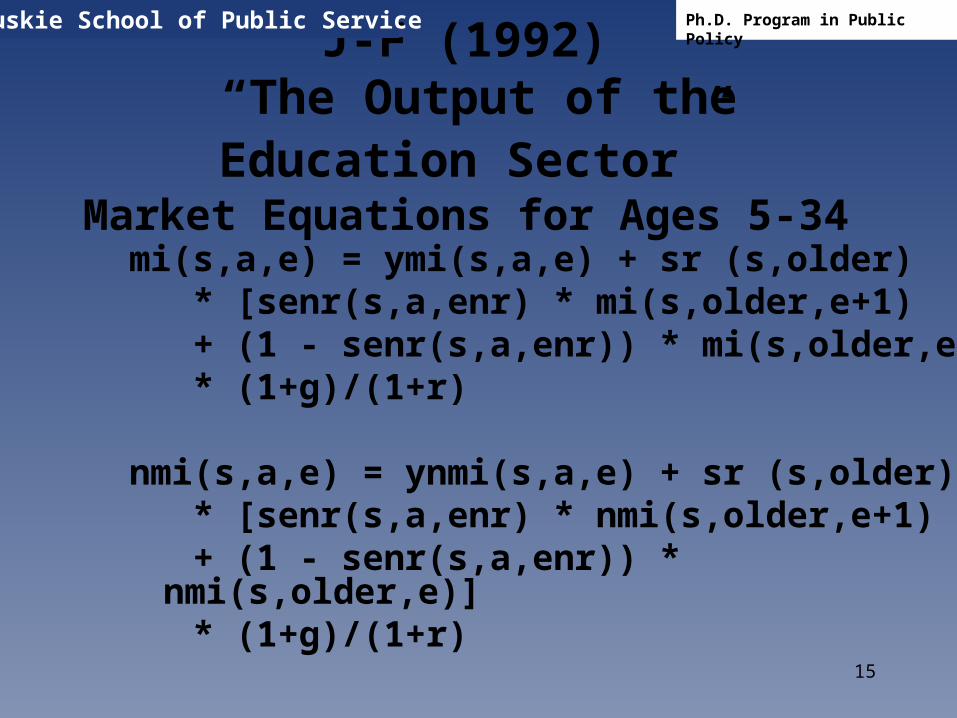
15
J-F (1992) “The Output of the Education Sector”
Market Equations for Ages 5-34
mi(s,a,e) = ymi(s,a,e) + sr (s,older) * [senr(s,a,enr) * mi(s,older,e+1) + (1 - senr(s,a,enr)) * mi(s,older,e)] * (1+g)/(1+r)
nmi(s,a,e) = ynmi(s,a,e) + sr (s,older) * [senr(s,a,enr) * nmi(s,older,e+1) + (1 - senr(s,a,enr)) * nmi(s,older,e)] * (1+g)/(1+r)
Muskie School of Public Service Ph.D. Program in Public Policy

16
Focus on implementation of the Fraumeni
simplified method
Muskie School of Public Service Ph.D. Program in Public Policy

17
Muskie School of Public Service Ph.D. Program in Public Policy
“Human capital accounting is simultaneously one of the easiest and most difficult exercises in empirical economics.
It is easy in the sense that the statistical
techniques necessary are relatively simple.
On the other hand, getting the data right can be massive challenge.”
Christian (2009)
18
Categorical Approach Challenges
• Finding data
• “Adjusting” the data
• Making reasonable assumptions
Muskie School of Public Service Ph.D. Program in Public Policy

19
Categorical Approach Major Issues
• School (and work?) years– Match between enrollment and age
categories– Progression, including assumptions– Age of enrollment
• Births
Muskie School of Public Service Ph.D. Program in Public Policy

20
Examples of Categorical ApproachesCanada
• In most cases individuals of a certain age are assumed to be enrolled in a specific grade determined by their current educational attainment level
• Individuals who are older individuals for a particular enrollment level are spread across grades
Muskie School of Public Service Ph.D. Program in Public Policy

21
Examples of Categorical ApproachesCanada
In the U.S., students in a particular pre-college grade are typically of two
different ages
Muskie School of Public Service Ph.D. Program in Public Policy

22
Examples of Categorical ApproachesNorway
Used years left to complete education
Muskie School of Public Service Ph.D. Program in Public Policy

23
Examples of Categorical ApproachesChina
• Have data on initial enrollment
• Used average probability of advancement to the next education level
• Labor income determined with Mincer equations
Muskie School of Public Service Ph.D. Program in Public Policy
24
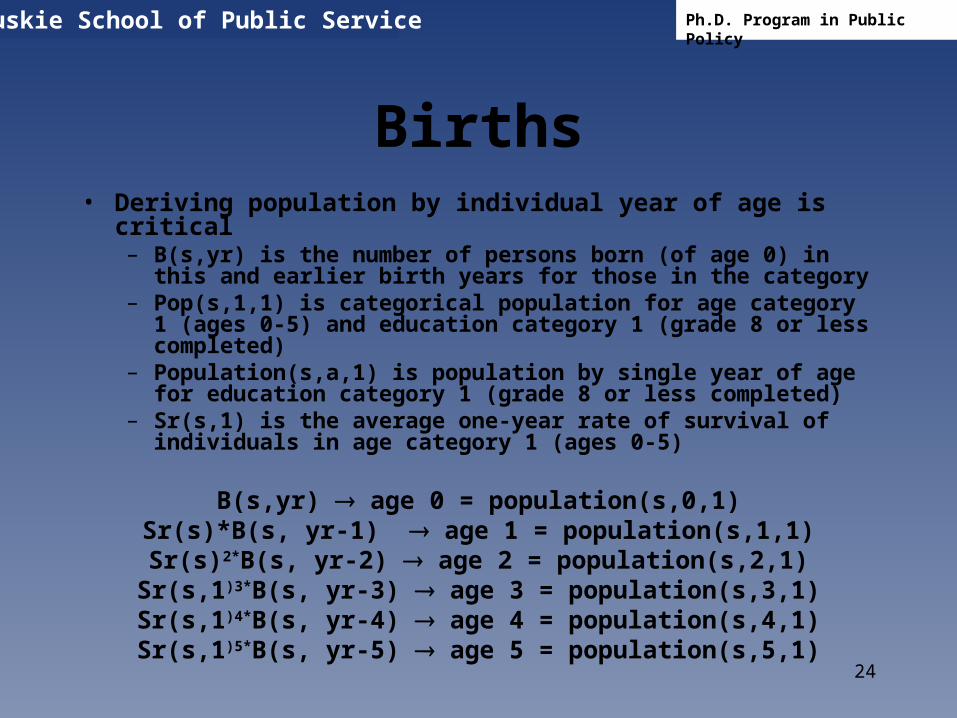
• Deriving population by individual year of age is critical– B(s,yr) is the number of persons born (of age 0) in this and earlier
birth years for those in the category– Pop(s,1,1) is categorical population for age category 1 (ages 0-5) and
education category 1 (grade 8 or less completed)– Population(s,a,1) is population by single year of age for education
category 1 (grade 8 or less completed)– Sr(s,1) is the average one-year rate of survival of individuals in age
category 1 (ages 0-5)
B(s,yr) age 0 = population(s,0,1)Sr(s)*B(s, yr-1) age 1 = population(s,1,1)Sr(s)2*B(s, yr-2) age 2 = population(s,2,1)
Sr(s,1)3*B(s, yr-3) age 3 = population(s,3,1)Sr(s,1)4*B(s, yr-4) age 4 = population(s,4,1)Sr(s,1)5*B(s, yr-5) age 5 = population(s,5,1)
Muskie School of Public Service Ph.D. Program in Public Policy
Births

25
Issues With This Birth Imputation
• Survival rates are taken from the current year
• The survival rate from age 0 to age 1 is typically significantly different from later ages survival rates
Muskie School of Public Service Ph.D. Program in Public Policy

26
Rose-colored glasses effect in the U.S.
Elsewhere?
Muskie School of Public Service Ph.D. Program in Public Policy

27
Country Success with J-F
The current efforts indicate that J-F can be done with categorical data
Data problems are being overcome
Looks good moving forward
Muskie School of Public Service Ph.D. Program in Public Policy