Comments Welcome

Ratings-Based Regulation and Systematic Risk Incentives

by

Giuliano Iannotta

Department of Economics and Business Administration Universitá Cattolica

Email: giuliano.iannotta@unicatt.it

and

George Pennacchi

Department of Finance University of Illinois

Email: gpennacc@illinois.edu

First Draft: August 2011 This Draft: September 2014

Abstract

When capital regulation is based on credit ratings, our model shows that a financial institution raises its shareholder value by selecting similarly-rated loans and bonds with the highest systematic risk. This moral hazard occurs if loan and bond credit spreads incorporate systematic risk premia not reflected in credit ratings. Our empirical evidence confirms that similarly-rated bonds have significantly greater credit spreads when their issuers have a higher systematic risk or “debt beta.” Moreover if a financial institution chooses higher-yielding, but equivalently-rated, bonds, its systematic risk and fair capital requirements rise by an economically significant amount. Our theory provides an explanation for prior research documenting that banks and insurance companies took excessive systematic risks.

An earlier version of this paper was titled “Bank Regulation, Credit Ratings, and Systematic Risk.” Valuable comments were provided by Tobias Berg, Timotej Homar, Christine Parlour, Andrea Resti, Francesco Saita, João Santos, Andrea Sironi, René Stulz, Andrew Winton and participants of the 2011 International Risk Management Conference, the 2011 Bank of Finland Future of Risk Management Conference, the 2012 Financial Risks International Forum, the 2012 Red Rock Conference, the 2012 FDIC Bank Research Conference, the 2012 Banque centrale du Luxembourg Conference, the 2013 Financial Intermediation Research Society Meetings, the 2013 Banco de Portugal Conference, and seminars at Copenhagen Business School, the Federal Reserve Banks of Cleveland and San Francisco, the Federal Reserve Board, HEC Paris, Imperial College, Indiana University, INSEAD, the Korea Deposit Insurance Corporation, Universitá Bocconi, Universitat Pompeu Fabra, the University of Tennessee, and Warwick Business School. We are very grateful to CAREFIN for providing financial assistance.

1. Introduction

Governments insure the liabilities of several financial institutions that invest in fixed-income

securities. Prime examples are federal government insurance of bank deposits and state government

guarantees of insurance company policies.1 One justification for guaranteeing these liabilities is that they are

held by unsophisticated individuals who cannot adequately judge the institutions’ default risks. Moreover, a

government, rather than private, guarantor may be warranted when the institutions are exposed to systematic

risks or their liabilities are subject to runs. These circumstances could lead to systemic financial institution

failures that only a government could credibly insure.

A consequence of providing guarantees is that financial institutions may have incentives to take

excessive risks. If unchecked, this moral hazard exposes governments to large losses from resolving

insolvent institutions. Regulation in the form of risk-based capital standards, and sometimes risk-based

insurance premiums, aims to neutralize these moral hazard incentives. However, the current regulatory

framework for banks and insurance companies might actually create a particular form of moral hazard. As

shown by Kupiec (2004) and Pennacchi (2006), risk-based capital requirements and premium assessments

that fail to differentiate between systematic and idiosyncratic risks can encourage systematic risk-taking; that

is, banks and insurance companies will have an incentive to make loans and invest in bonds that are highly

likely to suffer losses during an economic downturn.

The objective of our paper is to examine whether the use of credit ratings in setting regulatory

standards can promote this systematic moral hazard. We analyze, both theoretically and empirically, whether

an insured financial institution (IFI) might profitably exploit credit rating-based regulations. More

specifically, Basel II and III Accords base a bank’s required capital on either the external or internal credit

ratings of its loans and bonds. Similarly, the U.S. National Association of Insurance Commissioners (NAIC)

and European Solvency II standards set minimum capital based on the credit ratings of an insurance

company’s investments. If these ratings reflect differences in physical, but not risk-neutral, expected default

losses, we show that such regulation subsidizes an IFI’s relative cost of funding systematically risky

investments. The reason is that an IFI whose investments have high systematic default risk earns a large

systematic risk premium above the investments’ expected default losses. But this IFI does not pay a

1 Another example is federal government insurance of private defined-benefit pension plan retirement payments. Brown (2010) surveys various government insurance programs.

2

commensurate systematic risk cost on its government-insured liabilities if credit rating-based capital

standards or insurance premiums fail to penalize systematic risk. The IFI can exploit this subsidy and

increase its shareholder value simply by selecting the highest yielding loans and bonds within each

regulatory credit rating class.

The consequences of this credit rating-induced moral hazard are particularly devastating to financial

system stability. First, IFIs will herd into the most systematically risky investments, making simultaneous IFI

failures particularly sensitive to economic downturns. Second, IFIs will prefer to fund borrowers with high

systematic risk, misdirecting the economy’s allocation of capital toward excessively pro-cyclical projects.

Critical empirical questions regarding the validity of this moral hazard theory are whether credit spreads

indeed reflect systematic risk and, if so, whether credit ratings fail to account for this risk to the same degree.

Our paper’s theory predicts “reaching for yield” behavior: an inordinate preference by some investors

for high-yielding securities (Becker and Ivashina (2012)). It explains why IFIs subject to credit rating-based

regulations prefer debt whose yields reflect high systematic risk premia, though not necessarily high

expected default losses. Empirically, our paper develops an arguably superior measure of a corporate debt

security’s systematic risk and shows how this “debt beta” is an economically significant component of bond

yields. The paper also shows how one can calculate the required increase in fair capital when IFIs exploit this

regulatory arbitrage by reaching for yield.

A key distinction made in our paper is the difference in information reflected in a debt security’s credit

spread versus its credit rating, where a rating can derive from an IFI’s “internal” model or from an “external”

rating agency such as Moody’s or Standard & Poor’s (S&P). Asset pricing theory predicts that credit spreads

incorporate systematic risk premia to compensate investors for risk-neutral expected default losses. If ratings

were to reflect the same risk, then two debt issues that have the same probability of default (PD) and loss

given default (LGD) should have different ratings if one were more likely to experience default losses during

a macroeconomic downturn. In other words, ratings need to penalize systematic (undiversifiable) default

losses more than idiosyncratic (diversifiable) default losses. We argue that many internal ratings, including

Basel’s Internal Ratings-Based Approach, fail to reflect systematic risk differences across broad classes of

fixed-income securities.

Whether external credit rating agencies design their credit ratings to penalize systematic default risks is

3

not obvious and is the focus of our paper’s empirical tests. In the past, S&P stated that its credit ratings

reflect only PDs, but in 2010 it introduced a new stability criterion to its rating methodology (Standard &

Poor’s 2010): a lower rating is assigned if “an issuer or security has a high likelihood of experiencing

unusually large adverse changes in credit quality under conditions of moderate stress (for example,

recessions of moderate severity, such as the U.S. recession of 1982 and the U.K. recession in the early 1990s

or appropriate sector-specific stress scenarios).” S&P’s revision appears to be the first time that it explicitly

penalizes issuers for systematic, relative to nonsystematic, risk. Moody’s, whose ratings aim to reflect

expected default losses (PD×LGD), has not announced a similar revision.

Prior empirical evidence on whether credit spreads and ratings reflect systematic risk is limited. Elton,

Gruber, Agrawal, and Mann (2001) analyze average credit spreads on bonds grouped by rating class and by

maturity, and they find that monthly changes in spreads are significantly related to Fama and French (1993)

risk factors. Systematic risk factors also are found to explain individual corporate bonds’ monthly changes in

spreads (Collin-Dufresne, Goldstein, and Martin (2001)) and monthly excess returns (Schaefer and

Strebulaev (2008)).2 Closer to our paper is Hilscher and Wilson (2010) who find that S&P issuer ratings are

related to some measures of systematic default risk. They also find that systematic risk is strongly related to

bond credit spreads. However, none of these studies tests whether a bond’s credit spread reflects systematic

risk beyond that implied by its credit rating, which is the critical issue for the regulatory use of ratings.

Our paper begins by employing a standard structural credit risk model that shows why banks and

insurance companies have an incentive to invest in the most systematically risky loans and bonds if ratings-

based regulatory capital and guarantee premia fail to reflect differences in systematic risk. The model also

shows how the systematic risk of a loan or bond (debt beta) can be derived from the systematic risk of the

issuing firm’s stock (equity beta). To assess the realism of the model, we carry out three empirical exercises.

First, we examine whether credit spreads actually impound systematic risk, as measured by the issuer’s debt

beta, after controlling for credit ratings. Second, we investigate whether credit ratings reflect systematic risk,

either fully, partially, or not at all. Third, we consider the economic significance of the systematic risk

premium embedded in credits spreads and calculate the regulatory capital shortfall that occurs when an IFI

exploits credit ratings-based capital standards.

2 These findings do not establish that credit spreads embed a systematic risk premium since changes in credit spreads or returns may reflect changes in expected default losses that are correlated with systematic risk factors.

4

Our empirical analysis of credit spreads and credit ratings uses an international sample of 3,924 bonds

issued during the period from 1999 to 2010. The data comprise credit spreads and issue credit ratings at the

time that each bond is underwritten, along with characteristics of each bond and its issuer. Three main results

emerge that indicate there is scope for arbitrage of credit rating-based regulations when applied to corporate

debt. First, investors require significantly higher credit spreads on bonds issued by firms with relatively high

debt betas, even after controlling for the bond’s credit rating. Similarly, if a bank or insurance company

chooses bonds of a given credit rating class that have above median credit spreads, the systematic risk of its

investments rises by an economically significant amount. In contrast, we find that the idiosyncratic risk of

the issuer’s debt has no impact on credit spreads after accounting for credit ratings. As such, ratings do not

fully incorporate the issuer’s systematic risk, while they do capture idiosyncratic risk. These results are

robust to controlling for a bond’s illiquidity, to excluding bonds issued during the 2008 to 2010 financial

crisis, and to including only bonds rated by Moody’s or only bonds rated by S&P.

Second, after accounting for the total risk or idiosyncratic risk of an issuer’s debt, there is no evidence

in our overall sample that issuers with higher systematic risk are given a worse credit rating. However, if

bonds issued during the financial crisis are excluded, we find that ratings reflect an economically small

amount of the issuer’s systematic risk. Nonetheless, since we found that credit spreads incorporate a large

systematic risk premium after controlling for credit ratings, the implication is that rating agencies fail to

account for systematic risk to the same extent as investors. Third, the size of the systematic risk premium

embedded in bond spreads is consistent with standard asset pricing theory. Moreover, when IFIs reach for

yield by choosing bonds of a given rating class that have relatively high systematic risk, their regulatory

capital levels are lower than a fair level by an economically significant degree.

By demonstrating that credit spreads incorporate a systematic risk premium not accounted for by credit

ratings, our empirical work highlights the potential for profitably exploiting credit rating-based regulation.

While prior research such as Coval, Jurek, and Stafford (2009) has emphasized the high systematic risk

inherent in structured securities, we show that there is also scope for high systematic risk in corporate debt.

We review prior research and informal evidence that is consistent with banks and insurance companies

having an especial attraction to a variety of highly-rated but systematically-risky investments.

The paper proceeds as follows. Section 2 presents a model that shows why regulation based on credit

5

ratings gives IFIs incentives to take excessive systematic risk. Section 3 describes our data and presents

summary statistics. Section 4 investigates whether credit spreads reflect an issuer’s systematic risk while

Section 5 analyzes the impact of the issuer’s systematic risk on its credit ratings. Section 6 considers the size

of the systematic risk premium in credit spreads and its implication for fair capital standards. Section 7

discusses empirical evidence from other studies that relate to our model’s predictions, while Section 8

concludes.

2. A model of a regulated financial intermediary

This section illustrates why the current structure of ratings-based regulation creates incentives for

banks and insurance companies to take excessive systematic risk. Its model is similar to the binomial models

in Kupiec (2004) and Pennacchi (2006), but uses the standard continuous-time settings of Merton (1974,

1977), Galai and Masulis (1976), and Cummins (1988). This framework is better suited to guide our

empirical analysis which uses the “debt beta” measure of systematic risk that derives from the model. The

model is also used to compute an IFI’s capital shortfall when it exploits credit rating-based regulations.

2.1. Model assumptions

An IFI is assumed to invest in a portfolio of bonds and loans that it funds by issuing shareholders’

equity and government-insured liabilities. For concreteness, we refer to this IFI as a “bank” and its liabilities

as “deposits.” However, as discussed below, with minor modeling changes this IFI can be interpreted as an

“insurance company” and its liabilities as “insurance policies.”

At the initial date 0, the bank has insured deposits of D0 on which it pays the competitive, default-free

interest rate of r. Shareholders contribute equity capital equal to K0, so initially the bank has assets worth A0

= D0 + K0 that are invested in a portfolio of default-risky bonds and loans. These bonds and loans represent

the debt of firms in m industries that are exposed to different sources of risk. Each firm has a capital structure

that satisfies the assumptions in Merton (1974). If the bank maintains constant portfolio proportions invested

in the m different industries, Appendix A shows that the rate of return on the bank’s total assets is

,1

mtA i ii

t

dA dt dzA

dt dz

µ σ

µ σ

== +

= +

∑ (1)

6

where σA,i is the volatility of returns from the bank’s loans and bonds of firms in industry i, dzi is the

Brownian motion process specific to firm asset returns in industry i, dzidzj = ρijdt, 2, ,1

m m

A j A i ijj iσ σ σ ρ

== ∑ ∑ ,

and 1,1

m

A i iidz dzσ σ

=≡ ∑ . Assuming the Capital Asset Pricing Model (CAPM) holds, Appendix A shows that

the expected rate of return on the bank’s asset portfolio satisfies the relationship

1

mM i ii

rµ ϕ ω β=

= + ∑ (2)

where ϕM is the excess expected return on the market portfolio of all assets (or “equity premium”), ωi is the

bank’s proportion of total assets held in bonds and loans of firms in industry i, and βi is the average debt beta

of firms in industry i. Firms’ debt betas (and equity betas) are calculated based on Galai and Masulis (1976),

and details are given in Appendix A where equations (A.4) and (A.5) show that a firm’s debt beta is an

increasing function of its leverage, asset volatility, and asset beta.

A government regulator sets a risk-based capital standard and a deposit insurance premium for the

bank. The insurance premium is set at date 0 but payable at a future date T, which also is the time that the

regulator audits the bank. Let p be the (continuously-compounded) annual premium rate per deposit, so that

the bank’s total insurance premium to be paid at date T is DT(epT-1) and its total amount of deposits plus

premium payable at date T is DTepT = D0e(r+p)T .3 Similar to Merton (1977), if at the audit date AT < D0e(r+p)T,

the bank is declared to have failed and is closed or merged with another institution. The government

regulator/deposit insurer incurs any loss required to pay off insured deposits.

2.2. Fair insurance premiums and capital standards

There are three claimants on the bank’s assets: depositors, bank shareholders, and the government

regulator/insurer. Since insured depositors have a default-free claim paying the competitive rate r, the date 0

value of their claim is worth D0. Denote the date 0 values of claims on the bank’s assets by shareholders and

by the government regulator as E0 and G0, respectively. Then

0 0 0 0 0 0A D K D E G= + = + + (3)

or K0 = E0 + G0. When capital standards or deposit insurance premiums are set fairly, G0 = 0, so that E0 = K0

=A0 – D0; that is, the shareholders’ claim equals the funds that they contribute. If G0 < 0, so that E0 > K0, then

3 This insurance premium is analogous to a credit spread on deposits if deposits were uninsured. In the absence of deposit insurance and regulation, uninsured depositors would set the credit spread, p, to make the date 0 fair value of their default-risky deposits equal to D0, the amount they contribute initially.

7

a government subsidy transfers value to the shareholders. In general, the government’s claim equals

[ ] ( )( )( )

( ) ( )

0 0 0 0

0

E E max ,0

E min 1 ,

1 E max ,0

rT Q rT Q pTT T T T

rT Q pTT T T

pT rT Q pTT T

G A D E

e A D e A D e

e D e A D

D e e D e A

− −

−

−

= − −

= − − − = − −

= − − − (4)

where EQ[·] computes “risk-neutral” expectations of the bank’s assets.4 Equation (4) shows that the claim of

the government equals the value of its premium income, D0(epT – 1), minus the value of a put option written

on the bank’s assets, e-rTEQ[max(DTepT-AT ,0)]. If G0 = 0, indicating no subsidy, equation (4) implies:

( ) ( )( ) ( ) ( )

( )

0

0 2 0 0 1

0 0 0

1 E max ,0

, ,

pT rT Q pTT T

pT

pT

D e e D e A

D e N d K D N d

Put K D D e T

− − = − = − − + −

≡ +

(5)

where ( )( ) ( )21 0 0 0ln / /pTd K D D e T Tσ σ = + + , 2 1d d Tσ= − , and Put(A0,X,T) is the value of a

Black-Scholes put option written on assets current worth A0, having exercise price X, and time until maturity

of T. The key insight of equation (5) is that initial capital, K0, is set fairly when it produces risk-neutral

expected losses, ( )E max ,0rT Q pTT Te D e A− − = ( )0 0 0, ,pTPut K D D e T+ , equal to the value of the

government’s insurance premium, ( )0 1pTD e − .

Similar to Cummins (1988), equation (5) can be reinterpreted as the relationship between an insurance

company’s fair capital, K0, and its guaranty fund premium rate, p. D0 is now the initial value of the policies

underwritten by the company which equals the initial premiums paid by insured policyholders to the

company. However, unlike deposits, future policy values can be uncertain due to unexpected claims

experience. Let σD be the annualized standard deviation of the insurance company’s policyholder claims, and

let ρAD be the correlation between policyholders’ claims and the insurance company’s asset returns.5 Then

equation (5) continues to hold with σ2 replaced with 2 2 2 2I D AD Dσ σ σ ρ σσ≡ + − .

2.3. Actual insurance premiums and capital standards

4 The risk-neutral asset return process is / Qt tdA A rdt dzσ= + .

5 The risk-neutral process for insurance policy values is assumed to be /t t

QD DdD D rdt dzσ= + , where AD

Q QDdz dtdz ρ= .

8

To motivate how current regulation deviates from the fair standard (5), this section briefly overviews

the setting of premiums and capital requirements for U.S. and European Union (E.U.) banks and insurance

companies. A common feature is that regulation fails to account for differences in systematic risk across

broad asset classes due to internal or external ratings reflecting physical, not risk-neutral, expected losses.

2.3.1 Deposit insurance: Premium assessments differ across countries. The U.S. FDIC attempts to

calibrate a bank’s premium to cover the FDIC’s physical expected loss from the bank’s failure.6 In addition,

the overall level of premia is adjusted to target FDIC Deposit Insurance Fund (DIF) reserves, a policy that

Pennacchi (1999) shows is inconsistent with setting fair premia. Currently, the E.U. has a mix of deposit

insurance assessment schemes that generally are not risk-based. However, in December 2013 the European

Parliament agreed to move toward a common deposit insurance fund with an FDIC-like reserve target.7

2.3.2 Bank capital requirements: The U.S. and E.U. have implemented the recommendations of the

Basel Accords at different dates. Basel II and III are almost identical in terms of setting credit risk weights

for determining capital requirements, and they both include a “Standardized” approach (generally applicable

to smaller banks) and an “Internal Ratings-Based” (IRB) approach (applicable to larger banks). Large U.S.

banks transitioned from Basel I to the Basel III IRB in January 2014.8 The E.U. implemented the Basel II

Standardized approach in January 2007 and the IRB approach in January 2008.

Under the IRB approach, credit risk capital charges are based on internal ratings generated from the

single risk factor portfolio model analyzed in Gordy (2003). Inputs into the capital charge formula are the

bank’s own estimates of its bonds’ and loans’ physical probabilities of default (PD) and losses given default

(LGD).9 The Basel formula then converts these physical inputs into their hypothetical risk-neutral

6 For example, see Federal Register 76 (38) February 25, 2011 which amends the Federal Deposit Insurance Act to comply with the Dodd-Frank Act. An underlying principle for setting premiums (assessments) is stated on page 10700: “Under the FDI (Federal Deposit Insurance) Act, the FDIC’s Board of Directors must establish a risk-based assessment system so that a depository institution’s deposit insurance assessment is calculated based on the probability that the DIF (Deposit Insurance Fund) will incur a loss with respect to the institution.” The FDIC’s statistical failure probability models, on which its premium schedule is based, use physical, rather than risk-neutral, probabilities of bank failures. 7 The current FDIC DIF reserve target is between 1.35% and 1.50% of insured deposits. The EU target will be 0.8%. 8 With few exceptions, credit risk weights for small U.S. banks remain the same as Basel I. All corporate obligations are assigned a single 100% risk weight. 9 There is a “Foundation” IRB approach where LGD is fixed for corporate claims. For example, it is 45% for all senior, unsecured bonds and loans. Under the “Advanced” IRB approach, guidelines recommend that banks estimate a bond or loan’s “downturn” LGD which reflects losses that are expected to occur if default happens during an economic downturn. In principle, use of downturn LGDs may differentiate between high and low systematic risk claims, but since PDs are not conditioned on a downturn, the VaR capital requirement is unlikely to fully incorporate systematic risk.

9

counterparts using an assumed beta or market correlation for each asset class.10 Importantly, this assumed

beta (correlation) is not chosen by the bank but is set by Basel IRB rules and is essentially the same across

very broad asset classes.11 Hence, within an asset class, such as all corporate claims, there is no ability to

differentiate between high and low systematic default risk for debt securities having the same PD×LGD.

The Basel Standardized approach links a bond or loan’s capital charge to its external credit rating. For

corporate claims, credit risk weights are 20%, 50%, 100%, and 150% for bonds or loans rated AAA to AA-,

A+ to A-, BBB+ to BB-, and below BB-, respectively. Thus, for a given rating category, there is no scope for

distinguishing between high and low systematic risk bonds and loans, i.e. the capital charge for a given

rating category can reflect only a single level of systematic risk. The U.S. did not implement the

Standardized approach in part because the Dodd-Frank Wall Street Reform and Consumer Protection Act of

2010 mandated the removal of external credit ratings from all regulations. With few exceptions, small U.S.

banks’ credit risk weights remain the same as Basel I, which for corporate obligations is a single 100% risk

weight. Hence, there is no differentiation in systematic risk whatsoever across corporate bonds and loans.

Interestingly, in November 2001 while under Basel I, U.S. regulators implemented for all banks a type of

Standardized approach for structured securities, such as mortgage-backed securities (MBS) and asset-backed

securities (ABS). MBS and ABS tranches rated AAA to AA-, A+ to A-, BBB+ to BBB-, and BB+ to BB-

were assigned risk weights of 20%, 50%, 100%, and 200%, respectively. Hence, U.S. capital requirements

favored highly-rated structured securities relative to corporate bonds and loans.12

Rather than being subject to Basel’s aforementioned “credit” risk weights, fixed-income securities held

in a bank’s “trading book” are subject to a “market” risk capital requirement based on a Value-at-Risk (VaR)

calculation. However, even these calculations may rely on external credit ratings. For example, in 2008 the

10 Since ,, /i Mi i A i Mρ σω β σ= , where ρi,M is the correlation between the market risk factor and the asset class i’s return,

an assumption regarding the correlation ρi,M essentially is an assumption regarding the asset class’s beta. 11 IRB rules require sufficient initial capital, K0, such that there is no more than a 0.1% physical probability of losses exceeding this initial capital over a one-year horizon. The VaR capital requirement formula assumes correlations with the market risk factor (betas) that differ across classes of credit risky claims. In principle, these correlations could distinguish between claims with high and low systematic risk claims. However, correlation values are the same for broad classes of bonds and loans. For corporate bonds and loans, the correlation value varies between 8% and 24%, but the variation is a function only of the borrowing firm’s annual sales (greater for firms with more than €50 million in sales) and the bank’s estimated physical PD, where correlation is higher for lower PDs. See BCBS (2005). Fitch Ratings (2008) finds no empirical support for the IRB rule’s inverse relationship between PDs and portfolio correlation (systematic risk). As will be reported in our empirical work, neither do we find an inverse relationship between a firm’s systematic risk (debt beta) and its probability of default (as reflected in its credit rating). 12 Basel III’s Standardized approach continues to link structured securities to their credit ratings. Under Basel III, small U.S. banks are assigned risk weights for structured securities based on a “Simplified Supervisory Formula” described in http://www.federalreserve.gov/bankinforeg/basel/files/capital_rule_community_bank_guide_20130709.pdf .

10

Swiss Federal Banking Commission required that UBS report the key causes of its severe losses. UBS’s

report to shareholders (UBS, 2008) states that external credit ratings helped determine “the relevant product-

type time series to be used in calculating VaR” (p. 20). Moreover, an over-reliance on credit ratings, which

appears to be common in large banks, was found to be a primary cause of UBS’s losses as “a comprehensive

analysis of the portfolios may have indicated that the positions would necessarily perform consistent with

their ratings” (p. 39). RiskMetrics also sometimes advocates basing VaR calculations on an issuer’s rating.13

2.3.3 Insurance company guaranty fund assessments: U.S. states assess insurance companies for the

cost of resolving an insolvency that occurs in their state. Typically, premiums are not related to an individual

company’s risk and are assessed after an insolvency, though New York is an exception that sets rates on a

pre-insolvency basis. The E.U. has a variety of guarantee schemes, with most funded on a post-insolvency

basis. Only Germany sets risk-based premiums inversely related to a company’s excess equity capital.

2.3.4 Insurance company capital regulation: Similar to the Basel Standardized approach, the U.S.

NAIC sets capital requirements of 0.4%, 1.3%, 4.6%, 10.0%, 23.0%, and 30.0% for debt securities rated

AAA to A, BBB, BB, B, CCC, and CC and below, respectively.14 Current E.U. regulation (Solvency I) sets

capital requirements as a fraction of technical provisions (for life insurers) and turnover figures (for non-life

insurers) unrelated to investment risk. However, in 2016 the EU’s Solvency II standards will set capital

requirements based on the product of a bond’s risk factor and its duration. A bond’s risk factor is 0.9%,

1.1%, 1.4%, 2.5%, 4.5%, and 7.5% for bonds rated AAA, AA, A, BBB, BB, and B or below, respectively.15

2.4. Implications of actual versus fair regulation

To summarize the previous section, bank and insurance company guarantee assessments are risk-

insensitive or based on physical expected losses. Also, bank and insurance company capital required for a

given bond or loan is based on either an external credit rating or an internal credit rating linked to estimated

physical expected default losses. Importantly, conditional on either type of rating, there is no differentiation

of systematic risk across a broad asset class, such as all corporate obligations. If, like internal ratings,

13 As stated in Mina and Xiao (2001, p.42) “For example, in marking-to-market a cash flow from an instrument issued by the U.S. Treasury, Treasury rates will be used, while for a cash flow from a Aa-rated financial corporate bond, the financial corporate Aa zero rate curve will be a good choice if a firm-specific zero rate curve is not available.” 14 Until 2009, structured securities, such as MBS, were also classified according to their credit ratings. Afterwards, NAIC modified the risk assessment of such securities, and Becker and Opp (2014) argue that these new MBS capital standards do not even cover expected default losses nor account for systematic risk. 15 For example, a BBB-rated bond with a duration of 5 years would require 2.5%×5 = 12.5% capital.

11

external credit ratings primarily measure physical expected losses, then similarly-rated debt can have

potentially sizable differences in systematic risk. Indeed, our empirical work will present such evidence.

Now if ratings fail to differentiate degrees of systematic risk, the capital charge for a given rating can

be fair for only a single level of systematic risk or debt beta. Equivalently, the implicit fair beta reflected in

the capital charge for a given rating may differ from the true beta of an IFI’s loan or bond having that rating.

Consequently, while an IFI’s true expected rate of return on assets is1

mM i ii

rµ ϕ ω β=

= + ∑ in equation (2),

actual capital rules imply a different expected rate of return 1

mB M i ii

r Bµ ϕ ω=

= + ∑ where Bi is the average

fair beta implied by the ratings of the IFI’s loans or bonds of industry i. Hence, when actual capital standards

fail to distinguish differences in systematic risks for a given rating class, it may be that Bi ≠βi and µB ≠ µ.

Accounting for this disparity between true and capital regulation-implied betas of the IFI’s assets, the

actual relationship between premiums and regulatory capital satisfies:

( ) ( ) ( ) ( ) ( )( ) ( )( )

0 0 2 0 0 1

0 0 0

1

, ,

B

B

TpT pT B B

T pT

D e D e N d K D e N d

Put K D e D e T

µ µ

µ µ

−

−

− = − − + −

= + (6)

where ( ) ( )( ) ( )211 0 0 0 2ln / /B TB pT T Td K D e D eµ µ σ σ− = + + and 2 1

B B Td d σ= − . Note that in equation (6)

collapses to the fair relationship (5) when µB = µ. However, when µB ≠ µ, actual capital standards fail to

convert physical expected losses to the correct risk-neutral expected losses, and the relationship (6) reflects

the deviation, µ - µB. Thus, the actual regulatory relationship leads to the same Black-Scholes put option

pricing formula as (5) except that the underlying asset value ( )0 0K D+ is everywhere replaced with

( ) ( )0 0

B TK D e µ µ−+ . Because put options are decreasing functions of the value of their underlying assets,

when µ > µB the value of the put option in equation (6) is less than that in equation (5):

( ) ( )( ) ( )0 0 0 0 0 0 if , , , , BB

T pT pTPut K D e D e T Put K D D e Tµ µ µ µ− >+ < + (7)

An implication of inequality (7) is that when a regulator uses equation (6) to set assessment rates, p,

and capital standards, K0, they are lower than those implied by the fair, no-subsidy relationship in equation

(5). Consequently, equation (4) shows G0 < 0 and from equation (3) E0 = K0 – G0 > K0, so that the subsidy

accrues to the IFI’s shareholders. To verify this transfer of subsidy, note that shareholders’ equity equals

12

( )( )( ) ( ) ( )

0 0

0 0 1 0 2

E max ,0

r p TrT QT

pT

E e A D e

K D N d D e N d

+− = − = + −

(8)

and since ( ) ( )0 0 0 1/ 1 0E K K N d∂ − ∂ = − < and ( ) ( )0 0 0 2/ 0pTE K p pD e N d∂ − ∂ = − < , the difference between

the market value and book value of equity, E0 - K0, increases as initial capital and the insurance premium

declines. The greater is (µ - µB), the greater is the difference between the put options in (7) and the greater is

subsidy reflected in the market value of equity, E0 - K0.

It is now apparent that an IFI can increase the subsidy accruing to its shareholders by raising the

relative systematic risk of its bond and loan portfolio, ( )1

mB M i i ii

Bµ µ ϕ ω β=

− = −∑ , by selecting greater

portfolio weights, ωi, in industries where the average debt beta of firms is high relative to the debt beta

implied by capital standard ratings. Also, within an industry, the IFI can select those bonds and loans of

firms with relatively high debt betas, thereby raising the average relative debt beta in that industry, (βi - Bi).

Such portfolio decisions need not change the overall volatility of the asset portfolio, σ, but even if they do,

the relative subsidy for any given level of portfolio volatility, σ, still increases.

Our model implies that IFIs subject to ratings-based capital rules will intentionally engage in

regulatory arbitrage by taking excessive systematic risks that raise their shareholders’ value. But naïve IFIs

that focus only on capital standards and credit spreads may also be tempted to do the same. Why? Note that

controlling for physical expected default losses, bonds or loans with greater systematic risk will have larger

credit spreads or yields to maturity. This is because if the debt beta of the ith bond or loan is βi, its expected

rate of return is r + ϕMβi. All else equal (including expected default losses), higher systematic risk and debt

beta raises the expected rate of return of the bond or loan, which must lower its price relative to its promised

payment, thereby raising its yield and credit spread.

Thus, if a naïve IFI subject to credit rating-based capital charges simply chooses bonds and loans that

have the highest credit spread or yield for a given credit rating, it will automatically pick relatively high beta

bonds and loans. By simply selecting top-yielding bonds and loans within a given rating class, the IFI may

inadvertently be loading up on systematic risk and, in turn, receiving a greater government subsidy.

The model implies that IFIs will herd into systematically risky loans and investments, thereby creating

a systemically risky banking and insurance sectors. Other models predict that banks may choose common

13

exposures, though not necessarily by investing in assets with relatively high systematic risk. Penati and

Protopapadakis (1988) develop a model where banks are “bailed out” by the government if a sufficiently

high proportion of them become insolvent at the same time, where “bailout” means de facto government

insurance of the insolvent banks’ de jure uninsured liabilities (e.g., shareholders’ equity or subordinated

debt). As a result, banks have an incentive to over-invest in similar loans.16 Acharya and Yorulmazer (2007)

provide a rationale for why governments would grant such bailouts, even though they are time-inconsistent

policies: allowing many banks to simultaneously fail leads to insufficient surviving banks that could

efficiently deploy the failed banks’ assets. Many governments’ reactions to the recent financial crisis appear

to confirm these papers’ predictions. Several banks and insurance companies were bailed out by their

national governments through provisions that range from the guarantee of uninsured debt to equity capital

injections. Consistent with their models, one way that IFIs could achieve common exposures would be to

lend to borrowers with high systematic risk, since they tend to default together during economic downturns.

However, our argument is different from these papers’ “too many to fail” rationale for government

bailouts that create moral hazard by banks. Our model shows that capital charges or insurance premia based

on credit ratings can lead an individual IFI to take more systematic risk, even if other IFIs do not and even if

the IFI is not bailed out but is allowed to fail.17 An individual IFI chooses to do so because credit rating-

based regulation, which determines the IFI’s cost of insured liability funding, fails to discriminate between

defaults in good versus bad times. However, credits spreads on loans and bonds, which determine the IFI’s

revenue, do reflect the systematic risk of defaults.

The next sections consider the empirical validity of our model’s main assumptions and, hence, whether

credit rating-based regulation can be exploited. We examine the relationships between credit spreads, credit

ratings, and systematic risk based on an international sample of bonds which we now describe.

3. Data

We obtained data from DCM Analytics on corporate bonds issued over the years 1999 to 2010. The

data has information on each bond issuer (nationality, industry, etc.) and each bond’s characteristics (credit

spread, credit rating of the issue, years to maturity, face value, currency, etc.). Because this data contains

16 Their main example is banks’ aggressive lending to less developed countries (LDCs) during the late 1970s and early 1980s. In equilibrium, the incentive to herd in these LDC loans pushed interest rates below competitive levels. 17 Consequently, even if legislative reforms, such as the Dodd-Frank Act, prevented government bailouts of de jure uninsured liabilities, our theory predicts that IFIs would continue to herd into systematically risky investments.

14

issue ratings and credit spreads at the time of a bond’s issuance, it is ideal for testing whether credit ratings

and spreads incorporate similar information. This primary bond market data avoids problems of stale ratings:

issue ratings should impound all information available to the rating agency at the time of issuance, the same

time when the bond’s initial credit spread is set by investors.18

From an initial sample of 7,413 fixed-coupon, investment-grade bonds that were non-convertible, non-

perpetual, and non-callable, we used Bloomberg to attempt to match each bond’s ISIN code with the issuer’s

corresponding stock ISIN code. Our final matched sample consists of 3,924 bonds issued by 620 listed firms,

mostly from North America, Europe, and Japan. For each bond, we collected from Bloomberg the issuer’s

stock returns for the 52 weeks prior to the bond’s issuance date along with the contemporaneous weekly

returns of the MSCI World Index.19

The construction of each bond issuer’s debt beta, the key variable in our analysis, is based on Galai

and Masulis (1976) and is detailed in Appendix A. The procedure uses data on the issuer’s market value of

equity, the beta and total volatility of its stock returns, and balance sheet information on the issuer’s debt, to

infer the market value, beta, and total volatility of the issuer’s assets. In turn, this information on the issuer’s

asset characteristics allows us to calculate debt beta, the systematic risk faced by the firm’s bondholders:

( ) ( )( )

11

1D A E

N dA EN dD D N d

β β β−

= − = (10)

where A, D, E are market values and βA, βD, βE are betas of the firm’s assets, debt, and equity, respectively,

( ) ( ) ( )211 2ln / /d A B r σ σ ττ = + + , 2 1d d σ τ= − , σ is asset volatility, and B is the promised payment

on debt to be paid in τ years.20 Similarly, estimates of the total and residual volatilities of the issuer’s stock

returns are used to compute the debt’s total and residual volatilities, measures of total and idiosyncratic risk.

Note that all of our calculations regarding a bond issuer’s debt beta and debt residual volatility do not

use information on the new bond issue itself, but instead rely on the issuer’s stock market and balance sheet

information just prior to the bond issue. In principle, a bond’s debt beta and residual volatility could be

estimated from a time series of the bond’s post-issuance returns. However, since many bonds are traded

18 Other studies sometime use issuer ratings and secondary market bond spreads. Since ratings may become “stale” due to infrequent adjustments, new information may be reflected in secondary market spreads prior to ratings. 19 Our main findings are robust to using the issuer’s domestic stock index rather than the MSCI World Index. 20 Our estimates of debt beta assume τ = 10 years, though the paper’s results are robust to assuming a 5-year maturity.

15

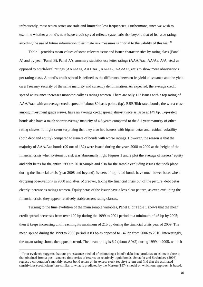
infrequently, most return series are stale and limited to low frequencies. Furthermore, since we wish to

examine whether a bond’s new-issue credit spread reflects systematic risk beyond that of its issue rating,

avoiding the use of future information to estimate risk measures is critical to the validity of this test.21

Table 1 provides mean values of some relevant issue and issuer characteristics by rating class (Panel

A) and by year (Panel B). Panel A’s summary statistics use letter ratings (AAA/Aaa, AA/Aa, A/A, etc.) as

opposed to notch-level ratings (AAA/Aaa, AA+/Aa1, AA/Aa2, AA-/Aa3, etc.) to show more observations

per rating class. A bond’s credit spread is defined as the difference between its yield at issuance and the yield

on a Treasury security of the same maturity and currency denomination. As expected, the average credit

spread at issuance increases monotonically as ratings worsen. There are only 132 issues with a top rating of

AAA/Aaa, with an average credit spread of about 80 basis points (bp). BBB/Bbb rated bonds, the worst class

among investment grade issues, have an average credit spread almost twice as large at 149 bp. Top-rated

bonds also have a much shorter average maturity of 4.8 years compared to the 8.1 year maturity of other

rating classes. It might seem surprising that they also had issuers with higher betas and residual volatility

(both debt and equity) compared to issuers of bonds with worse ratings. However, the reason is that the

majority of AAA/Aaa bonds (99 out of 132) were issued during the years 2008 to 2009 at the height of the

financial crisis when systematic risk was abnormally high. Figures 1 and 2 plot the average of issuers’ equity

and debt betas for the entire 1999 to 2010 sample and also for the sample excluding issues that took place

during the financial crisis (year 2008 and beyond). Issuers of top-rated bonds have much lower betas when

dropping observations in 2008 and after. Moreover, taking the financial crisis out of the picture, debt betas

clearly increase as ratings worsen. Equity betas of the issuer have a less clear pattern, as even excluding the

financial crisis, they appear relatively stable across rating classes.

Turning to the time evolution of the main sample variables, Panel B of Table 1 shows that the mean

credit spread decreases from over 100 bp during the 1999 to 2001 period to a minimum of 46 bp by 2005;

then it keeps increasing until reaching its maximum of 215 bp during the financial crisis year of 2009. The

mean spread during the 1999 to 2005 period is 83 bp as opposed to 147 bp from 2006 to 2010. Interestingly,

the mean rating shows the opposite trend. The mean rating is 6.2 (about A/A2) during 1999 to 2005, while it

21 Prior evidence suggests that our pre-issuance method of estimating a bond’s debt beta produces an estimate close to that obtained from a post-issuance time series of returns on relatively liquid bonds. Schaefer and Strebulaev (2008) regress a corporation’s monthly excess bond return on its excess stock (equity) return and find that the estimated sensitivities (coefficients) are similar to what is predicted by the Merton (1974) model on which our approach is based.

16

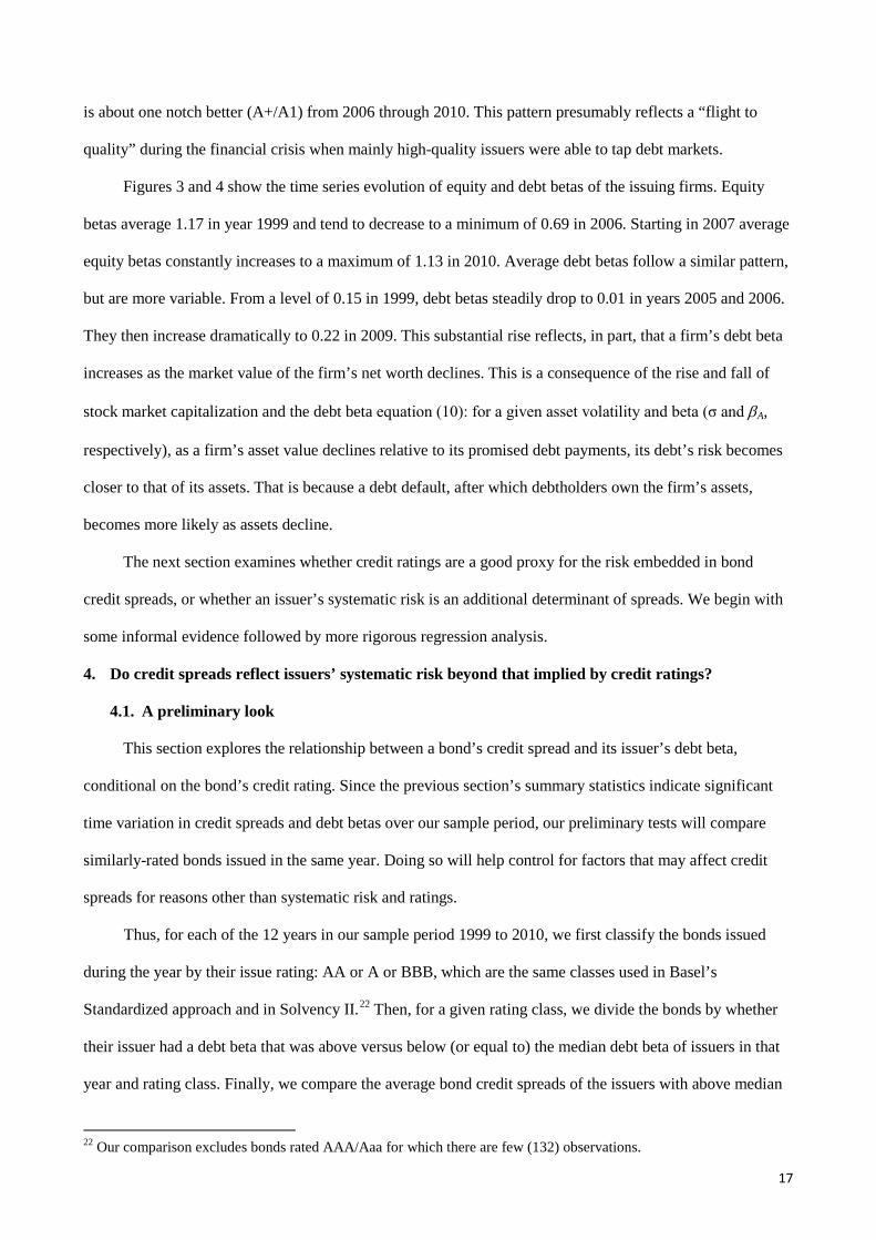
is about one notch better (A+/A1) from 2006 through 2010. This pattern presumably reflects a “flight to

quality” during the financial crisis when mainly high-quality issuers were able to tap debt markets.

Figures 3 and 4 show the time series evolution of equity and debt betas of the issuing firms. Equity

betas average 1.17 in year 1999 and tend to decrease to a minimum of 0.69 in 2006. Starting in 2007 average

equity betas constantly increases to a maximum of 1.13 in 2010. Average debt betas follow a similar pattern,

but are more variable. From a level of 0.15 in 1999, debt betas steadily drop to 0.01 in years 2005 and 2006.

They then increase dramatically to 0.22 in 2009. This substantial rise reflects, in part, that a firm’s debt beta

increases as the market value of the firm’s net worth declines. This is a consequence of the rise and fall of

stock market capitalization and the debt beta equation (10): for a given asset volatility and beta (σ and βA,

respectively), as a firm’s asset value declines relative to its promised debt payments, its debt’s risk becomes

closer to that of its assets. That is because a debt default, after which debtholders own the firm’s assets,

becomes more likely as assets decline.

The next section examines whether credit ratings are a good proxy for the risk embedded in bond

credit spreads, or whether an issuer’s systematic risk is an additional determinant of spreads. We begin with

some informal evidence followed by more rigorous regression analysis.

4. Do credit spreads reflect issuers’ systematic risk beyond that implied by credit ratings?

4.1. A preliminary look

This section explores the relationship between a bond’s credit spread and its issuer’s debt beta,

conditional on the bond’s credit rating. Since the previous section’s summary statistics indicate significant

time variation in credit spreads and debt betas over our sample period, our preliminary tests will compare

similarly-rated bonds issued in the same year. Doing so will help control for factors that may affect credit

spreads for reasons other than systematic risk and ratings.

Thus, for each of the 12 years in our sample period 1999 to 2010, we first classify the bonds issued

during the year by their issue rating: AA or A or BBB, which are the same classes used in Basel’s

Standardized approach and in Solvency II.22 Then, for a given rating class, we divide the bonds by whether

their issuer had a debt beta that was above versus below (or equal to) the median debt beta of issuers in that

year and rating class. Finally, we compare the average bond credit spreads of the issuers with above median

22 Our comparison excludes bonds rated AAA/Aaa for which there are few (132) observations.

17

debt betas to those of the issuers who were below or equal to the median. Hence, this comparison of credit

spreads by debt beta controls for not only the bonds’ rating class but also yearly time variation in spreads.

The first row of Panel A in Table 2 reports the results of this exercise by rating class. It gives the

average credit spreads of bonds issued by firms that had above and below the median debt betas in the year

the bonds were issued. For example comparing AA-rated bonds, the average credit spread for issuers whose

debt beta was above the median in the year of issue was 97.6 basis points while that of issuers whose debt

beta was below the median in the year of issue was 78.9 basis points, a statistically significant difference of

18.7 basis points. Similar findings occur for A and BBB-rated bonds: there is a positive, statistically

significant difference between the credit spreads of high and low debt beta issuers.

We repeated this comparison but using only bonds denominated in the same currency. Rows 2 to 5 of

Panel A, Table 2 report results from bonds denominated in Euros, U.S. dollars, Japanese yen, or British

pounds. The results we found when aggregating bonds across currencies generally hold on a currency by

currency basis. In only two of the 12 currency-rating classifications are the differences in credit spreads

between high and low debt beta issuers not positive and statistically significant, and in these two exceptions

the numbers of observations are relatively small. The last two rows of Panel A, Table 2 perform a similar

exercise but on subsamples of bonds whose maturities were above and below the median maturity in their

rating class and year. The qualitative result that credit spreads of bonds are higher when its issuer has a

relatively high debt beta appears to hold for both long- and short-maturity bonds.

In summary, Panel A of Table 2 suggests that similarly-rated bonds have higher credit spreads when

their issuer has a relatively high debt beta. Next, consider a related but different question: Are bonds with

relatively high credit spreads issued by firms with relatively high debt betas? To answer this, we repeat the

previous exercise but on a year-by-year basis sort similarly-rated bonds by whether their credit spreads were

above versus below the median for that rating class in that year. We then compare for each rating and year

the average debt betas of issuers whose bonds had above- versus below-median credit spreads.

The first row of Panel B, Table 2 reports the results for all AA, A, and BBB rated bonds. There we see

that, for each rating class, there is a positive and statistically significant difference between the debt betas of

issuers whose bonds had above median credit spreads versus those whose bonds had below median credit

spreads. The results generally hold for subsamples of bonds having a given currency denomination, as well

18

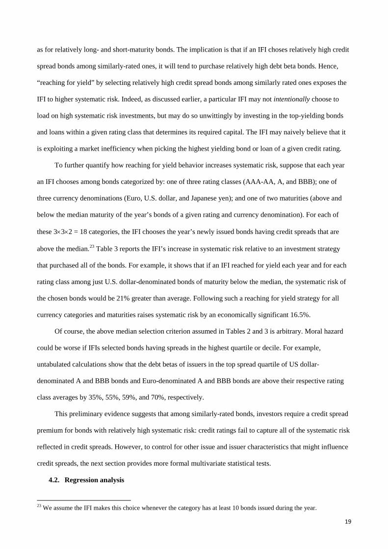
as for relatively long- and short-maturity bonds. The implication is that if an IFI choses relatively high credit

spread bonds among similarly-rated ones, it will tend to purchase relatively high debt beta bonds. Hence,

“reaching for yield” by selecting relatively high credit spread bonds among similarly rated ones exposes the

IFI to higher systematic risk. Indeed, as discussed earlier, a particular IFI may not intentionally choose to

load on high systematic risk investments, but may do so unwittingly by investing in the top-yielding bonds

and loans within a given rating class that determines its required capital. The IFI may naively believe that it

is exploiting a market inefficiency when picking the highest yielding bond or loan of a given credit rating.

To further quantify how reaching for yield behavior increases systematic risk, suppose that each year

an IFI chooses among bonds categorized by: one of three rating classes (AAA-AA, A, and BBB); one of

three currency denominations (Euro, U.S. dollar, and Japanese yen); and one of two maturities (above and

below the median maturity of the year’s bonds of a given rating and currency denomination). For each of

these 3×3×2 = 18 categories, the IFI chooses the year’s newly issued bonds having credit spreads that are

above the median.23 Table 3 reports the IFI’s increase in systematic risk relative to an investment strategy

that purchased all of the bonds. For example, it shows that if an IFI reached for yield each year and for each

rating class among just U.S. dollar-denominated bonds of maturity below the median, the systematic risk of

the chosen bonds would be 21% greater than average. Following such a reaching for yield strategy for all

currency categories and maturities raises systematic risk by an economically significant 16.5%.

Of course, the above median selection criterion assumed in Tables 2 and 3 is arbitrary. Moral hazard

could be worse if IFIs selected bonds having spreads in the highest quartile or decile. For example,

untabulated calculations show that the debt betas of issuers in the top spread quartile of US dollar-

denominated A and BBB bonds and Euro-denominated A and BBB bonds are above their respective rating

class averages by 35%, 55%, 59%, and 70%, respectively.

This preliminary evidence suggests that among similarly-rated bonds, investors require a credit spread

premium for bonds with relatively high systematic risk: credit ratings fail to capture all of the systematic risk

reflected in credit spreads. However, to control for other issue and issuer characteristics that might influence

credit spreads, the next section provides more formal multivariate statistical tests.

4.2. Regression analysis

23 We assume the IFI makes this choice whenever the category has at least 10 bonds issued during the year.

19

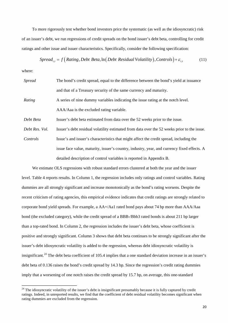
To more rigorously test whether bond investors price the systematic (as well as the idiosyncratic) risk

of an issuer’s debt, we run regressions of credit spreads on the bond issuer’s debt beta, controlling for credit

ratings and other issue and issuer characteristics. Specifically, consider the following specification:

( )( ), ,, , ln ,i t i tSpread f Rating Debt Beta Debt Residual Volatility Controls ε= + (11)

where:

Spread The bond’s credit spread, equal to the difference between the bond’s yield at issuance

and that of a Treasury security of the same currency and maturity.

Rating A series of nine dummy variables indicating the issue rating at the notch level.

AAA/Aaa is the excluded rating variable.

Debt Beta Issuer’s debt beta estimated from data over the 52 weeks prior to the issue.

Debt Res. Vol. Issuer’s debt residual volatility estimated from data over the 52 weeks prior to the issue.

Controls Issue’s and issuer’s characteristics that might affect the credit spread, including the

issue face value, maturity, issuer’s country, industry, year, and currency fixed effects. A

detailed description of control variables is reported in Appendix B.

We estimate OLS regressions with robust standard errors clustered at both the year and the issuer

level. Table 4 reports results. In Column 1, the regression includes only ratings and control variables. Rating

dummies are all strongly significant and increase monotonically as the bond’s rating worsens. Despite the

recent criticism of rating agencies, this empirical evidence indicates that credit ratings are strongly related to

corporate bond yield spreads. For example, a AA+/Aa1 rated bond pays about 74 bp more than AAA/Aaa

bond (the excluded category), while the credit spread of a BBB-/Bbb3 rated bonds is about 211 bp larger

than a top-rated bond. In Column 2, the regression includes the issuer’s debt beta, whose coefficient is

positive and strongly significant. Column 3 shows that debt beta continues to be strongly significant after the

issuer’s debt idiosyncratic volatility is added to the regression, whereas debt idiosyncratic volatility is

insignificant.24 The debt beta coefficient of 105.4 implies that a one standard deviation increase in an issuer’s

debt beta of 0.136 raises the bond’s credit spread by 14.3 bp. Since the regression’s credit rating dummies

imply that a worsening of one notch raises the credit spread by 15.7 bp, on average, this one-standard

24 The idiosyncratic volatility of the issuer’s debt is insignificant presumably because it is fully captured by credit ratings. Indeed, in unreported results, we find that the coefficient of debt residual volatility becomes significant when rating dummies are excluded from the regression.

20

deviation higher debt beta impacts the spread only slightly less than would a notch downgrade.

Earlier we noted that bonds issued during the financial crisis have better issue ratings, notwithstanding

a remarkably higher systematic risk. The association between good ratings and high systematic risk observed

from 2008 to 2010 might bias our results, leading to an over-estimate of the systematic risk premium

required by investors. Thus, Column 4 of Table 2 reports results of a regression that excludes bonds issued in

the years 2008 and beyond. Two main findings emerge.

First, the premiums for lower quality ratings relative to a AAA/Aaa rating are much smaller for all

rating notch classes, reflecting the ease of tapping debt markets in the pre-crisis era. For example, while in

the whole sample the average BBB-/Bbb3 bond pays about 208 bp more than a AAA/Aaa rated bond,

excluding the financial crisis the figure drops to 76 bp, roughly the same as a AA+/Aa1 in the whole sample.

In addition, when excluding the financial crisis a AA+/Aa1 bond does not have a significantly higher credit

spread than a top-rated bond. In particular, credit spreads for the whole AA/Aa rating class (including bonds

with ratings equal to AA+/Aa1, AA/Aa2, AA-/Aa3) are not statistically different from that of a AAA/Aaa

bond if we exclude 2008 to 2010. Therefore, it seems that in the pre-crisis era bond investors relied on credit

ratings mostly to discriminate between just the best and the worst of investment-grade bonds. This result is

relevant for capital regulation. Under Basel II/III, claims rated from AAA to AA- have the same risk weight

(20% for claims on corporates).25 Our evidence suggests this standard holds in “normal” times, but in times

of stress investors discriminate between a AAA bond and each notch-level rating within the AA class.

Second, although strongly significant, the coefficient on debt beta is smaller compared to the whole

sample regression (67.8 versus 108.8). Thus, it is plausible that investors required a greater systematic risk

premium during the financial crisis. Column 5 reports a regression that interacts a dummy variable for the

financial crisis years (2008-10) and the issuer’s debt beta. As expected, the interaction term is positive and

strongly significant, suggesting that the market price of systematic risk rose after 2008.26

4.3. Controlling for liquidity

Spreads between corporate bonds and Treasuries may reflect not only credit risk but also illiquidity.

The regressions reported in Table 4 controlled for a number of issue characteristics, including the issue size,

25 There is even less granularity under U.S. NAIC regulations, as the least risk category that is given a 0.3% capital charge includes bonds with ratings from AAA to A. 26 This is consistent with Berg (2010) who analyzes the term structure of credit default swap (CDS) spreads and finds a rise in the short-term market price of systematic risk during the financial crisis.

21

which should proxy for a bond’s secondary market liquidity. However, if for some reason bonds of issuers

with high debt betas were less liquid, they might be priced less at issuance and have higher spreads. Thus,

since credit ratings do not account for bond liquidity, what our previous regression analysis of credit spreads

presumes to be a systematic risk premium might actually be an illiquidity risk premium. We now address this

concern with an additional test that controls for a bond’s observed illiquidity in the secondary market. A

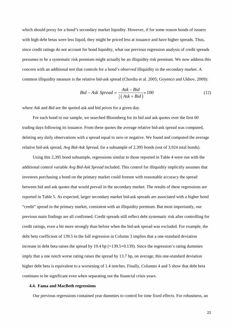
common illiquidity measure is the relative bid-ask spread (Chordia et al. 2005; Goyenco and Ukhov, 2009):

( )12

100Ask BidBid Ask SpreadAsk Bid

−− = ×

+ (12)

where Ask and Bid are the quoted ask and bid prices for a given day.

For each bond in our sample, we searched Bloomberg for its bid and ask quotes over the first 60

trading days following its issuance. From these quotes the average relative bid-ask spread was computed,

deleting any daily observations with a spread equal to zero or negative. We found and computed the average

relative bid-ask spread, Avg Bid-Ask Spread, for a subsample of 2,395 bonds (out of 3,924 total bonds).

Using this 2,395 bond subsample, regressions similar to those reported in Table 4 were run with the

additional control variable Avg Bid-Ask Spread included. This control for illiquidity implicitly assumes that

investors purchasing a bond on the primary market could foresee with reasonable accuracy the spread

between bid and ask quotes that would prevail in the secondary market. The results of these regressions are

reported in Table 5. As expected, larger secondary market bid-ask spreads are associated with a higher bond

“credit” spread in the primary market, consistent with an illiquidity premium. But most importantly, our

previous main findings are all confirmed. Credit spreads still reflect debt systematic risk after controlling for

credit ratings, even a bit more strongly than before when the bid-ask spread was excluded. For example, the

debt beta coefficient of 139.5 in the full regression in Column 3 implies that a one-standard deviation

increase in debt beta raises the spread by 19.4 bp (=139.5×0.139). Since the regression’s rating dummies

imply that a one notch worse rating raises the spread by 13.7 bp, on average, this one-standard deviation

higher debt beta is equivalent to a worsening of 1.4 notches. Finally, Columns 4 and 5 show that debt beta

continues to be significant even when separating out the financial crisis years.

4.4. Fama and MacBeth regressions

Our previous regressions contained year dummies to control for time fixed effects. For robustness, an

22

alternative method for controlling time variation is presented. Using similar specifications and variables as in

the prior regressions, we now run year-by-year Fama and MacBeth (1973) - style regressions. Table 6 reports

the average of the year-by-year regression coefficients along with robust standard errors clustered at the

issuer level. The results are remarkably consistent with those of the earlier regressions. In all of the credit

spread specifications, the coefficient on debt beta is positive and statistically significant while that on debt

residual volatility is not. This is true whether a bid-ask spread control for bond illiquidity is included or not.

4.5. Regressions with only Moody’s or only S&P ratings

In our previous regressions, the dummy variables for the bond’s issue rating at the notch level reflected

the average of its Moody’s and S&P rating when both were available. When only one agency rated the bond,

just that rating was used. Hence, the rating control reflected a blend of both Moody’s and S&P ratings. To

see whether our results are sensitive to using only Moody’s ratings or only S&P ratings, we reran regressions

on subsamples of Moody’s-rated and S&P-rated bonds. The results are reported in Table 7. The subsample

of bond rated by S&P is somewhat larger than that of Moody’s, whether or not the bond sample is restricted

to those having a bid-ask spread control for bond illiquidity. That said, the results are not qualitatively

different. As before, debt beta is a positive and statistically significant predictor of credit spreads, while debt

residual volatility is not. Hence, whether one controls for Moody’s rating or S&P’s rating does not change

the influence of debt beta on credit spreads.

To sum up, our results suggest that credit spreads required by bond investors incorporate systematic

risk beyond that reflected in credit ratings. In contrast, once one controls for credit ratings, credit spreads do

not appear to reflect the issuer’s idiosyncratic risk. Put another way, credit ratings seem to be based on

physical expected default losses, while investors value bonds based on risk-neutral expected default losses.

However, we cannot reject the hypothesis that ratings at least partially impound information about the

issuer’s systematic risk. Indeed, it is possible that investors assign a different weight to systematic risk than

raters do. In the next section we investigate whether issue ratings reflect issuers’ systematic risk by running

regressions of ratings on the issuers’ debt betas, volatilities, and other issue and issuer controls.

5. Do credit ratings reflect issuers’ systematic risk?

Statements by credit rating agencies suggest that issue ratings reflect a bond’s physical probability of

default, as would be true if ratings measured the issuer’s overall default likelihood and not how default states

23

are split between economic expansions versus economic recessions. If, instead, ratings differentiated

between idiosyncratic and systematic default states, they might reflect risk-neutral probabilities of default if

defaults in bad economic states were weighted relatively greater.

Both Moody’s and S&P claim that normal fluctuations in economic activity and the consequent effects

on the credit quality of an issuer or issue are impounded into their credit ratings. In other words, ratings are

assigned “through the cycle.” Whether this approach includes an assessment of systematic risk is unclear. On

the one hand, an evaluation of the possible adverse consequences of an economic slowdown on a credit

rating would arguably imply an analysis of the bond’s systematic risk. On the other hand, if raters place

probabilities on the likely occurrence of different economic scenarios equal to their physical (actual), rather

than risk-neutral, probabilities, then their calculations of expected default or expected default losses will not

equal risk-neutral expected default or default losses. For example, an issuer with high systematic risk might

be considered extremely vulnerable to a recession, but if the probability of a recession is not weighted

greater than its physical probability, ratings will not reflect risk-neutral expected default losses.

Recently, S&P announced new ratings criteria (Standard & Poor’s, 2008, 2010) that suggests it may

switch from using physical default probabilities to something akin to risk-neutral ones. The President of

S&P, Deven Sharma, summarized this change with the statement “Under S&P’s new criteria,…we may feel

that two securities have similar default risk, but if we believe one is more prone to a sharp downgrade in

periods of economic stress, it will be rated lower initially.” Such a rating methodology might have the

potential to place greater weight on default losses during an economic downturn.

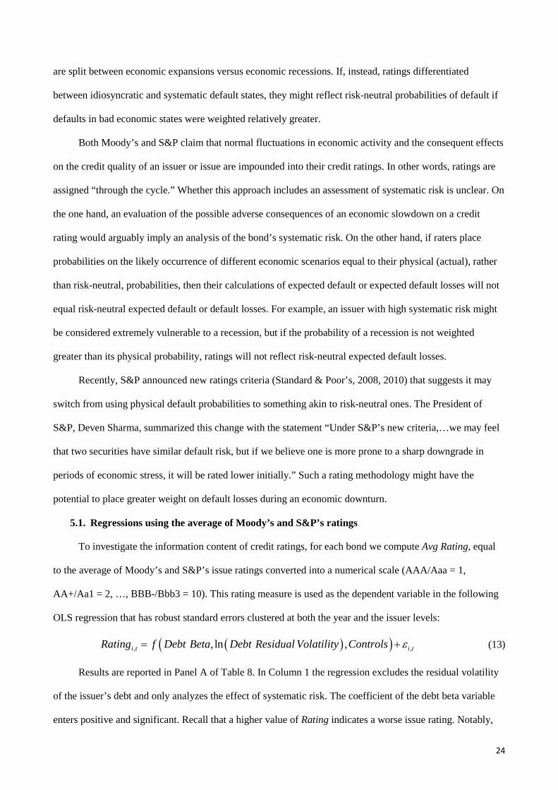
5.1. Regressions using the average of Moody’s and S&P’s ratings

To investigate the information content of credit ratings, for each bond we compute Avg Rating, equal

to the average of Moody’s and S&P’s issue ratings converted into a numerical scale (AAA/Aaa = 1,

AA+/Aa1 = 2, …, BBB-/Bbb3 = 10). This rating measure is used as the dependent variable in the following

OLS regression that has robust standard errors clustered at both the year and the issuer levels:

( )( ), , , ln ,i t i tRating f Debt Beta Debt Residual Volatility Controls ε= + (13)

Results are reported in Panel A of Table 8. In Column 1 the regression excludes the residual volatility

of the issuer’s debt and only analyzes the effect of systematic risk. The coefficient of the debt beta variable

enters positive and significant. Recall that a higher value of Rating indicates a worse issue rating. Notably,

24

however, when including the issuer’s idiosyncratic risk, the debt beta becomes insignificant (Column 2).

Results are very similar when replacing the idiosyncratic (residual) volatility of the issuer’s debt with the

total volatility of the issuer’s debt (Column 3).

As noted earlier, two effects of the financial crisis on the bond market are clearly detectable in our

sample: i) primarily high credit quality issuers could access the market, resulting in better average issue

ratings; and ii) the systematic risk of issuers increased dramatically. As a result, during the crisis high-quality

bonds are associated with very high issuer debt betas, therefore possibly biasing our results towards the

finding that ratings do not account for systematic risk. Indeed, by focusing on the sub-sample of bonds issued

before 2008, a different picture emerges. Ratings do reflect systematic risk (Column 4), even when

controlling for the residual or total volatility of the issuer’s debt (Columns 5 and 6). However, the effect is

economically small. For example, based on the debt beta coefficient of 1.682 in Column 5, a one standard

deviation increase in debt beta worsens the rating by only 0.18 of a notch (=1.682×0.1079). In contrast, the

previous section’s results show that a one-standard deviation increase in debt beta raised the spread by an

amount equivalent to about one full notch or more. The results imply that raters may partially account for

systematic risk, but not nearly as much as bond investors.

Our use of Avg_Rating as the dependent variable in an OLS regression implicitly assumes that ratings

are cardinal measures of risk; that is, the risk difference between rating classes is constant. It also reflects a

discrete, granular scale that may not accurately reflect the regression’s continuous explanatory risk variables.

To see if these issues may drive our results, we now consider an ordered probit regression. To limit the

number of cases in the dependent variable, we round the Avg_Rating variable to the closest integer. Results,

reported in Columns 7 and 8 of Panel A in Table 8, confirm our previous findings. Excluding bonds issued

during the financial crisis, issue ratings reflect both systematic and either idiosyncratic or total risk.

5.2. Regressions using only Moody’s rating or only S&P’s rating

As mentioned previously, S&P recently announced a change in its rating methodology, introducing a

criterion based on stability (Standard & Poor’s, 2008, 2010). Now ratings (both issuer and issue) are assigned

based on the current credit quality and also on the rating’s expected stability in a stress scenario. According

to this newly adopted criterion, S&P’s ratings should reflect the tendency of a firm’s (or security’s) credit

quality to deteriorate in bad times. Moody’s did not react to the S&P’s announcement with an analogous

25

change in its rating criteria. This might introduce a wedge between the two agencies over ratings assigned

from 2008 on. Alternatively, it is possible that Moody’s already assessed systematic risk to some extent. To

check whether raters differ in their assessment of systematic risk, we run regressions of ratings on debt beta

by using Moody’s and S&P’s ratings separately. Results, reported in Columns 1-8 of Panel B of Table 8, are

similar to those obtained in the previous section. When dropping bonds issued during the financial crisis,

both Moody’s and S&P reflect issuers’ systematic risk.

6. Implications of our empirical results for bond risk premia and capital standards

6.1. The premium for bond systematic risk

The CAPM, extended to account for illiquidity premia, predicts that the promised yield to maturity on

a default-risky bond, y, is approximately

D My r PD LGD ip β ϕ= + × + + × (14)

where r is the yield on an equivalent maturity default-free bond, PD is the annualized physical probability of

default (default intensity), LGD is the proportional physical loss given default, ip is an illiquidity premium,

βD is the bond’s debt beta, and ϕM is the excess expected return on the market portfolio of all assets. Our tests

in Section 4 regressed credit spreads, y – r, on credit ratings and other issuer and issue control variables. If,

as our empirical findings suggest, ratings primarily capture physical expected default losses, PD × LGD, and

other controls (such as the bond’s bid-ask spread) capture illiquidity premia, ip, then the term βD × ϕM should

capture systematic risk. Indeed, the regression coefficient on the bond’s debt beta βD can be interpreted as an

estimate of the excess return on the market portfolio, ϕM, assumingϕM is constant over time.

For example, in Table 5 which includes bonds’ bid-ask spreads as a control for illiquidity, the

coefficient on debt beta for the benchmark regression in Column (3) is 139.5. Since the regression’s credit

spreads are in basis points, this estimate translates to an estimate of ϕM = 1.395%. Multiplying this by the

sample’s average debt beta of βD = 0.099 implies that the average systematic risk premium for the sample’s

bonds is βD × ϕM = 0.138% or 13.8 basis points.27

This estimate of ϕM = 1.395% is lower than U.S. stocks’ historical “equity premium” of around 8%,

27 Similarly, if in Column 3 of Table 5 the product of Avg Bid-Ask Spread and its coefficient of 90.4 is assumed to account for the liquidity risk premium, ip, then given the sample average of 0.278 for Avg Bid-Ask Spread, the bond sample’s average liquidity risk premium is 90.4×0.278 = 25.2 basis points.

26

though such a high historical equity risk premium may be a puzzle.28 However, there is evidence that ϕM may

not be constant since the regression in Column (5) indicates that it rose to a value of ϕM = (2.9963 + 0.6514)

= 3.65% during the financial crisis years 2008-2010.

There are theoretical reasons why the systematic risk premium reflected in bonds might be less than

that reflected in stocks. If, as our model predicts, IFIs choose fixed-income securities having relatively high

systematic risk (debt beta), their extraordinary demand may affect these securities’ equilibrium risk premia.

For example, if different types of debt securities were in perfectly inelastic supply, greater demand for

securities with systematically-risky payoffs would bid up their prices and lower their yields, reducing the

premium for systematic risk reflected in their yields. Conversely, if debt securities with systematically-risky

payoffs were in perfectly elastic supply, greater IFI demand would generate greater supply with no reduction

in these securities’ systematic risk premia.29 This issue is relevant because banks fund a high proportion of

loans and insurance companies are major investors in corporate bonds.30 However, there is likely to be some

elasticity in the supply of systematically-risky, but highly-rated debt. The growth in the supply of highly-

rated, structured securities may have been a response to greater demand (Coval, Jurek, and Stafford, 2009).

Moreover, there are empirical reasons why our estimate of ϕM is likely to be downward biased. Based

on equation (10), each bond’s debt beta was calculated from an estimate of the issuing firm’s stock beta and

volatility, as well as the firm’s debt-to-equity ratio. Arguably, this procedure is superior to estimating betas

from a time-series of bond returns because bonds tend to be much less liquid than stocks and their debt betas

display more time variation compared to equity betas (Figures (3) and (4)).31 Still, there is estimation error in

our construction of debt beta, which is well known to produce a downward biased coefficient estimate.

Suggestive evidence of this bias is the higher debt beta coefficient that was obtained using the subsample of

bonds for which bid-ask spreads are available. The firms that issue such bonds are likely to have relatively

28 Each year, the Federal Reserve Bank of Philadelphia’s Survey of Professional Forecasters (http://www.phil.frb.org/research-and-data/real-time-center/survey-of-professional-forecasters/ ) reports forecasts of the return on the U.S. S&P500 over the next ten years, as well as forecasts of U.S. Treasury bill returns over the next ten years. The difference between these two forecasts provides a forecast of the equity premium. The difference in the mean forecasts over the 1999 to 2010 period was 3.65%, significantly lower than the historical time series average. 29 Perfectly inelastic supplies would correspond to an endowment economy such as Lucas (1978), while perfectly elastic supplies would correspond to a production economy such as Cox, Ingersoll, and Ross (1985). 30 Bord and Santos (2012) report that in 2007, banks’ approximate shares of syndicated credit lines and term loans were 92% and 44%, respectively. For the year 2010, Becker and Ivashina (2012) note that U.S. life insurance companies were the single largest investors in corporate bonds which represented 39% of their portfolios, and Fitch Ratings (2011) report that corporate bonds represented 35% of E.U. insurance companies’ assets. 31 Studies of bond returns, such as Bao and Pan (2013) who use TRACE data and Schaefer and Strebulaev (2008) who use Merrill Lynch data, are limited to constructing monthly returns due infrequent bond trading.

27

liquid and transparent stock prices, reducing the estimation error when calculating their debt betas.

6.2. Capital deficits from exploiting ratings-based capital standards

This section addresses the following issue. Suppose ratings-based capital standards are calibrated to

the average systematic risk for the universe of fixed-income securities in a given rating class. However, an

IFI exploits these capital standards by choosing among similarly-rated securities those with higher than

average systematic risk. How much would capital requirements need to be raised in order to fairly reflect the

IFI’s higher systematic risk?

Consider the situation of a U.S. commercial bank using the model and parameter estimates in

Pennacchi (2005). The parameter estimates derive from a sample of 42 large, publically-traded banks. The

model is the same as that in Section 2 but modified in two ways to better characterize a large U.S. bank.

First, when a bank fails (its end of period assets are less than liabilities), the cost to the government insurer is

3.2% of liabilities, which is the FDIC’s average loss rate for large banks. Second, the model is multi-period

in that the single-period model of Section 2 is repeated for multiple year-length periods: banks that are

solvent at the end of each year partially adjust their capital ratios back to a target level, where capital mean-

reverts such that capital deviations from target are expected to decline by 17.7% over the next year.

Our capital calibrations use the average annual asset/liability volatility from this 42 bank sample of σ =

3.14%. We then suppose that ratings-based target capital requirements would be set fairly for this bank if the

bank chose fixed-income securities with the average debt beta of B. However, we assume the bank actually

chooses fixed-income securities with having an average debt beta of β. Thus, as in the model of Section 2,

the bank earns an excess systematic risk premium of µ - µB = (β-B)×ϕM. We then calculate how much higher

target capital requirements would need to be when (β-B) equals 0.136, which is one standard deviation of the

debt betas in our corporate bond sample, and ϕM = 5%, which is higher than our downward biased regression

estimate but lower than the historical equity premium.

The calibration assumes that target capital requirements are set so that a steady state average deposit

insurance premium of p = 10 basis points is fair, similar to equation (5). However, regulators may adjust a

solvent bank’s actual insurance premium each year as its capital deviates from target. Assuming that each

year regulators adjust a bank’s deposit insurance premium to a fair level that fully reflects the bank’s capital

deviation from target, then the government’s liability is that of a limited-term, annual contract. Under this

28

assumption, we calculate that the bank’s choice of higher beta securities require 6.3% greater target capital.

However, in practice deposit insurance premiums are slow to adjust to changes in bank capital. If we

continue to assume that target capital requirements are set so that a steady state average deposit insurance

premium of p = 10 basis points is fair, but regulators adjust premiums to a fair level with a five-year moving

average, then the government’s liability is no longer that of a one-year limited-term contract. Under this

alternative, arguably more realistic assumption, we calculate that the bank’s choice of higher beta securities

would require a 16.0% higher target level of capital, an economically significant increase.

7. Direct empirical evidence on systematic moral hazard

The empirical work in previous sections of this paper tests and confirms a critical assumption of our

model, namely, that corporate bond credit spreads embed a systematic risk premium not accounted for by

credit ratings. It shows that this risk premium is economically significant and creates scope for regulatory

arbitrage if IFIs reach for yield by choosing high credit spread bonds among similarly-rated corporate bonds.

Previous empirical work has documented that other fixed-income securities, in particular senior

tranches of structured securities, also can have high systematic default risk. These securities include highly-

rated MBS, ABS, and collateralized debt obligations (CDOs). Coval, Jurek, and Stafford (2009) show that

the pooling of loans and bonds diversifies away idiosyncratic risks and exposes the senior tranches of these

securitized pools to mainly systematic default risk.32 However, they present empirical evidence that the

credit spreads on these highly-rated tranches failed to adequately reflect systematic risk because investors

mistakenly focused on the securities’ high ratings and low physical expected default losses. But using a

different calibration methodology, Collin-Dufresne, Goldstein, and Yang (2012) present opposite evidence

that these securities’ credit spreads did fully incorporate systematic risk. Evidence consistent with structured

securities’ yields embedding high systematic risk is Chernenko, Hanson, and Sunderam (2014) who find that,

prior to the financial crisis, the average yields on AAA-rated non-prime residential MBS and CDOs were

higher by 18 bp and 30 bp, respectively, compared to the average yield on AAA-rated corporate bonds.

Merrill, Nadauld, and Strahan (2014) also estimate that the average yields on AAA-rated structured

securities were almost 36 bp higher than the average yield on AAA-rated corporate bonds.33

32 Using a different model, Wojtowicz (2011) arrives at a similar result for collateralized bond obligations. 33 These yield comparisons presume that a given rating (e.g., AAA) measures the same default risk (e.g., physical expected losses) for both structured securities and corporate bonds. However, some research has argued that ratings for

29

Having presented evidence consistent with yields on corporate bonds and structured securities

containing systematic risk premia, the remainder of this section summarizes prior empirical research relevant

to our model’s prediction that IFIs subject to ratings-based capital regulation will prefer systematically-risky

investments. We start with empirical evidence for banks followed by evidence for insurance companies.

As mentioned earlier in Section 2.3.2, in 2001 U.S. bank regulators lowered the risk weights on AAA-

and AA-rated securitizations to 20% while the risk weights on all corporate obligations remained at 100%.

Given their generally higher spreads and lower capital charges, highly-rated structured securities appear to

have offered U.S. banks the best opportunity to exploit the regulatory arbitrage illustrated by our model.34

Some supporting evidence is a U.S. Government Accountability Office (GAO, 2013) investigation of the 414

U.S. bank failures from 2008 and 2011. It concluded that in about 10% of the small- and medium-sized bank

failures, losses on private label MBS and Fannie Mae and Freddie Mac preferred stock were a factor.

Evidence in Erel, Nadauld, and Stulz (2014) suggests that large banks who were active underwriters of

securitizations may have retained the highly-rated, but systematically risky, tranches of these securitizations

on their balance sheets due to the securities’ low 20% risk-weighting.35 However, prior to the crisis large

banks could earn the sizable systematic risk premium on highly-rated structured securities at an even lower

effective capital charge. This was done by funding these securities off-balance sheet in asset-backed

commercial paper conduits supported by the sponsoring bank’s lines of credit. Acharya, Schnabl, and Suarez

(2013) document that these credit lines backing the commercial paper were de facto credit guarantees but

qualified as liquidity guarantees for regulatory capital purposes. As a result, the conduit’s securities obtained

a capital risk weighting equal to only 10% of the capital charge had the securities been on-balance sheet.

Regulators in several European countries also permitted similar capital relief, explaining why many

European banks sponsored asset-backed commercial paper conduits that invested in structured securities.

Turning to insurance companies, they permit a more powerful test of our model predictions because,

relative to banks, insurance companies are subject to more detailed reporting of their security holdings. As

noted in Section 2.3.4, U.S. insurance companies were subject to external ratings-based capital standards that

structured securities were particularly inflated. As we discuss next, U.S. bank capital standards particularly favored highly-rated structured securities relative to similarly-rated corporate obligations. Opp, Opp, and Harris (2013) and Cole and Cooley (2014) argue that the increased regulatory reliance on ratings was the primary cause of this ratings inflation. 34 Stanton and Wallace (2012) also note that U.S. bank capital requirements particularly favored highly-rated MBS. 35 In the absence of their low capital charges it would be puzzling if banks retained these highly-rated senior tranches. Models of optimal securitization contracts, such as Pennacchi (1988), predict that banks would retain the most junior tranches (equity) to give them greater incentives to efficiently screen and monitor the securitized loan pool.

30

applied equally to corporate bonds and structured securities. Becker and Ivashina (2012) compare the

corporate bond holdings of insurance companies to those of mutual funds and pension funds, where the latter

two types of intermediaries are not subject to regulatory capital requirements. They find that, for a given

regulatory rating class, insurance companies own a higher proportion of bonds that have above average

credit spreads.36 Moreover, the tendency to select bonds with the highest spreads in a given rating class is

greater for insurance companies with more binding regulatory capital constraints. Furthermore, they show

that the insurance companies that chose high-yielding bonds were exposed to greater systematic risk.

Merrill, Nadauld, and Strahan (2014) provide complementary evidence on U.S. insurance companies’

holdings of structured securities. They find that when interest rates declined in the early 2000s and led to

losses in insurance companies’ annuities underwriting, the companies with the greatest capital declines

shifted their portfolios to highly-rated structured securities. The shift occurred only in these companies’

“general account” (which is subject to capital requirements) and not in their “separate accounts” (which are

not). The authors argue that this behavior is consistent with the relatively high credit spreads and low capital

requirements of highly-rated structured securities. Chernenko, Hanson, and Sunderam (2014) provide

additional evidence showing that holdings of high-yielding structured securities were greater for those U.S.

insurance companies that were poorly capitalized and organized as stock, rather than mutual, companies.

In summary, a variety of empirical evidence from both banking and insurance is consistent with our

model’s prediction that IFIs subject to ratings-based capital standards have incentives to invest in

systematically-risky, high credit spread assets.

8. Conclusions

This paper’s model predicts that if a debt security’s credit spread embeds a systematic default risk

premium that is not reflected in the debt’s credit rating, then rating-based regulation creates incentives for

IFIs to take excessive systematic risks. Complementing previous literature that emphasized the high

systematic risk of structured securities, this paper demonstrates that corporate bond credit spreads also can

contain economically significant systematic risk premia. It introduces a new empirical measure of a bond’s

systematic risk, the issuer’s debt beta, and show that it is an important component of a bond’s credit spread

36 As an example, they report that among newly issued bonds in the AAA to A regulatory rating class, insurance companies purchase 75% of bonds in the lowest spread quartile and 82% of bonds in the highest spread quartile, and this difference is statistically significant.

31

after accounting for the bond’s rating.

Since 2009, reforms to bank and insurance company capital requirements have concentrated on

structured securities and largely ignored corporate debt.37 With greater risk weights on structured securities,

corporate bonds and loans might now be the preferred vehicle for IFIs to engage in regulatory arbitrage. Our

empirical finding of significant variation in corporate bonds’ systematic risks shows that there remains scope

for IFIs to exploit ratings-based regulation.

What regulatory reforms might address this moral hazard? One reform advocated by some academics

and regulatory economists is to reduce the distortions of directly regulating IFIs by placing greater reliance

on market discipline.38 When an IFI obtains subordinated funding from investors who are not de jure or de

facto insured by a government, this uninsured debt’s credit spread should account for the IFI’s systematic

risk and act as a deterrent.39 In turn, regulatory capital requirements and supervisory actions might better

respond to systematic risk if they were linked to the credit spreads or credit default swap spreads of the IFI’s

uninsured debt, as Hart and Zingales (2010) advocate. In addition, decreasing the reliance on credit ratings

may be beneficial if an improved risk measure can be substituted. Indeed, as our analysis suggests, greater

use of credit spreads on loans and securities for setting capital requirements and insurance premiums

represents a likely improvement.40 Finally, more emphasis on setting capital requirements based on the

outcome of stress tests is a welcome regulatory innovation.41 By focusing on performance during severe

economic and financial downturns, the most systematically risky IFIs might be identified for greater required

capital.

37 Under Basel III, the Basel Committee (2009) has raised risk weights for securitizations and resecuritizations (e.g., CDOs) under both the Standardized approach and for the IRB approach. Also, NAIC no longer sets capital based on a structured security’s external rating. Thus far Basel III and NAIC recommend no major changes for risk weights on corporate claims relative to the standards set before the crisis. 38 See Flannery (1998) for a review. 39 In our model if an intermediary issued uninsured debt, its credit spread, p, would satisfy the fair standard equation (5). One approach to implement greater market discipline would be to narrow the scope of activities that could be funded by insured liabilities. Non-qualifying activities would need to be funded with uninsured funds in separate subsidiaries or separate firms. Examples of this approach are the 2010 Dodd-Frank Act’s “Volker Rule” that bars proprietary trading by banks, the 2011 U.K. Independent Commission on Banking’s (Vickers) proposal to restrict deposit-insured banks to “ring-fenced” retail and payments-related activities, and the 2012 European Commission High-Level Expert Group (Liikanen) Report’s proposal to restrict propriety trading and other risky activities non-bank, uninsured subsidiaries. 40 Credit spreads may be refined to adjust for possible liquidity and tax effects. Empirical evidence by Morgan and Ashcraft (2003) finds that credit spreads on a bank’s loans are a superior predictor of future bank distress. 41 Examples include the U.S.’s Comprehensive Capital Analysis and Review (CCAR) and the European Banking Authority’s EU-Wide Stress Test.

32

References

Acharya, V., Schnabl, P., and Suarez, G., 2013. Securitization without risk transfer. Journal of Financial

Economics 107, 515-536.

Acharya, V., and Yorulmazer, T., 2007. Too many to fail – An analysis of time-inconsistency in bank

closure policies. Journal of Financial Intermediation 16, 1-31.

Bao, J., and Pan, J., 2013. Bond illiquidity and excess volatility. Review of Financial Studies 26, 3068-3103.

Basel Committee on Banking Supervision, 2005. An Explanatory Note on the Basel II IRB Risk Weight

Functions. Bank for International Settlements.

_________________, 2009. Enhancements to the Basel II framework. Bank for International Settlements.

Becker, B., and Ivashina, V., 2012. Reaching for yield in the bond market. Journal of Finance (forthcoming).

Becker, B., and Opp, M., 2014. Regulatory reform and risk-taking. Swedish School of Economics and

University of California, Berkeley working paper.

Berg, T., 2010. The term structure of risk premia: New evidence from the financial crisis. Working Paper no.

1165, European Central Bank.

Bord, V., and Santos, J., 2012. The rise of the originate-to-distribute model and the role of banks in financial

intermediation. Federal Reserve Bank of New York Policy Review (July), 21-34.

Brown, J., 2010. Public Insurance and Private Markets, AEI Press, Washington, D.C.

Chernenko, S., Hanson, S., and Sunderam, A., 2014. The rise and fall of securitization. Harvard University

and Ohio State University working paper.

Chordia, T., Sarkar, A., and Subrahmanyam, A., 2005. An empirical analysis of stock and bond market

liquidity. Review of Financial Studies 18, 85-129.

Cole, H., and Cooley, T., 2014. Rating agencies. Working Paper 19972. National Bureau of Economic

Research.

Collin-Dufresne, P., Goldstein, R., and Martin, J., 2001. The determinants of credit spread changes. Journal

of Finance 56, 2177-2207.

Collin-Dufresne, P., Goldstein, R., and Yang, F., 2012. On the relative pricing of long-maturity index options

and collateralized debt obligations. Journal of Finance 67, 1983-2014.

33

Coval, J., Jurek, J., and Stafford, E., 2009. Economic catastrophe bonds. American Economic Review 99,

628-666.

Cox, J., Ingersoll, J., and Ross, S., 1985. An intertemporal general equilibrium model of asset prices.

Econometrica 53, 363-384.

Cummins, J.D., 1988. Risk-based Premiums for Insurance Guaranty Funds. Journal of Finance 43, 823-839.

Elton, E., Gruber, M., Agrawal, D., and Mann, C., 2001. Explaining the rate spread on corporate bonds.

Journal of Finance 56, 247-277.

Erel, I., Nadauld, T., and Stulz, R., 2014. Why did holdings of highly rated securitization tranches differ so

much across banks? Review of Financial Studies 27, 404-453.

Fama, E., and French, K., 1993. Common risk factors in the returns on stocks and bonds. Journal of

Financial Economics 33, 3-57.

Fama, E., and MacBeth J., 1973. Risk, Return and Equilibrium: Empirical Tests. Journal of Political

Economy 81 (3), 607-636.

Fitch Ratings, 2008. Basel II Correlations Values. Credit Market Research Financial Institutions Special

Report.

Fitch Ratings, 2011. Solvency II set to reshape asset allocation and capital markets. Insurance Rating Group

Special Report.

Flannery, M., 1998. Using market information in prudential bank supervision: A review of the U.S. empirical

evidence. Journal of Money, Credit and Banking 30, 273-305.

Fons, J., 2002. Understanding Moody’s corporate bond ratings and rating process. Moody’s Investors Service

Special Comment.

Galai, D., and Masulis, R., 1976. The option pricing model and the risk factor of stock. Journal of Financial

Economics 3, 53-81.

Gordy, M., 2003. A risk-factor model foundation for ratings-based bank capital rules. Journal of Financial

Intermediation 12, 199-232.

Government Accountability Office, 2013. Financial institutions: Causes and consequences of recent bank

failures. Report to Congressional Committees GAO-13-71,

34

Goyenco, A.D., and Ukhov, R.Y., 2009. Stock and bond market liquidity: A long-run empirical analysis.

Journal of Financial and Quantitative Analysis 44, 189-212.

Hart, O., and Zingales, L., 2009. A new capital regulation for large financial institutions. Harvard University

and University of Chicago working paper.

Hilscher J., and Wilson, M., 2010. Credit ratings and credit risk. Brandeis University working paper.

Kupiec, P., 2004. Is the new Basel Accord incentive compatible? In: Gup, B. (Ed.), The New Basel Capital

Accord. Thompson South-Western Publishers.

Lucas, R., 1978. Asset prices in an exchange economy. Econometrica 46, 1429-1445.

Marcus, A., and Shaked, I., 1984. The valuation of FDIC deposit insurance using option-pricing estimates.

Journal of Money, Credit and Banking 16, 446-460.

Merton, R., 1974. On the pricing of corporate debt: The risk structure of interest rates. Journal of Finance

29, 449-470.

Merton, R., 1977. An analytic derivation of the cost of deposit insurance and loan guarantees: An application

of modern option pricing theory. Journal of Banking and Finance 1, 3-11.

Merrill, C., Nadauld, T., and Strahan, P., 2014. Final demand for structured finance securities. Boston

College and Brigham Young University working paper.

Mina, J., and Xiao, J.Y., 2001. Return to RiskMetrics: The evolution of a standard. RiskMetrics Technical

Document.

Morgan, D., and Ashcraft, A., 2003. Using loan rates to measure and regulate bank risk: Findings and an

immodest proposal. Journal of Financial Services Research 24, 181-200.

Opp, C., Opp, M., and Harris, M., 2013. Ratings agencies in the face of regulation. Journal of Financial

Economics 108, 46-61.

Penati, A., and Protopapadakis, A., 1988. The effect of implicit deposit insurance on banks’ portfolio choices

with an application to international overexposure. Journal of Monetary Economics 21, 107–126.

Pennacchi, G., 1988. Loan sales and the cost of bank capital. Journal of Finance 43, 375-96.

Pennacchi, G., 1999. The effects of setting deposit insurance premia to target insurance fund reserves.

Journal of Financial Services Research 16, 63-90.

35

Pennacchi, G., 2005. Risk-based capital standards, deposit insurance, and procyclicality. Journal of

Financial Intermediation 14, 432-465.

Pennacchi, G., 2006. Deposit insurance, bank regulation, and financial system risk. Journal of Monetary

Economics 53, 1–30.

Schaefer, S., and Strebulaev, I., 2008. Structural models of credit risk are useful: Evidence from hedge ratios

on corporate bonds. Journal of Financial Economics 90, 1-19.

Standard & Poor’s, 2008. General criteria: Standard & Poor’s to explicitly recognize credit stability as an

important rating factor. (October 15) Available at www.standardandpoors.com.

Standard & Poor’s, 2010. General criteria: Methodology: Credit stability criteria. Available at

www.standardandpoors.com.

Stanton, R., and Wallace, N., 2012. CMBS subordination, ratings inflation, and regulatory-capital arbitrage.

University of California, Berkeley, working paper.

UBS, 2008. Shareholder report on UBS’s write-downs. Available at www. ubs.com.

Wojtowicz, M., 2011. CDOs and the financial crisis: Credit ratings and fair premia. VU University

Amsterdam working paper.

36

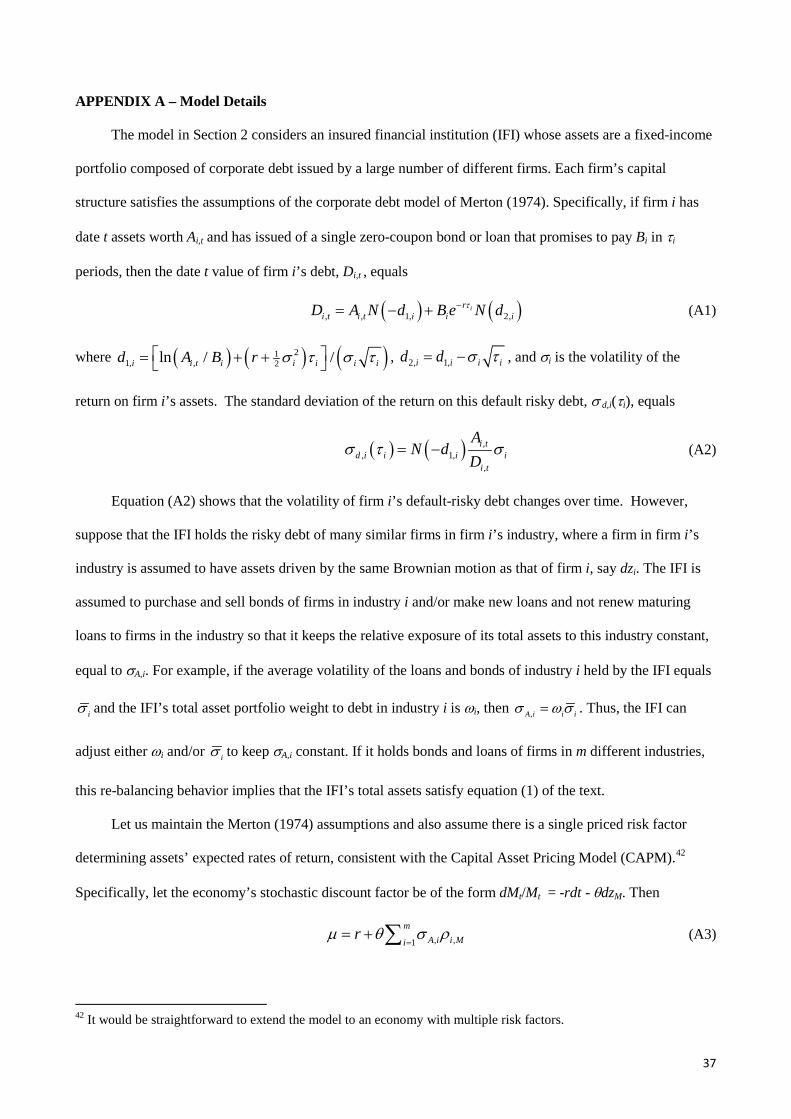
APPENDIX A – Model Details

The model in Section 2 considers an insured financial institution (IFI) whose assets are a fixed-income

portfolio composed of corporate debt issued by a large number of different firms. Each firm’s capital

structure satisfies the assumptions of the corporate debt model of Merton (1974). Specifically, if firm i has

date t assets worth Ai,t and has issued of a single zero-coupon bond or loan that promises to pay Bi in τi

periods, then the date t value of firm i’s debt, Di,t , equals

( ) ( ), , 1, 2,ir

i t i t i i iD A N d B e N dτ−= − + (A1)

where ( ) ( ) ( )211, , 2ln / /i i t i i i i id A B r σ τ σ τ = + + , 2, 1,i i i id d σ τ= − , and σi is the volatility of the

return on firm i’s assets. The standard deviation of the return on this default risky debt, σ d,i(τi), equals

( ) ( ) ,, 1,

,

i td i i i i

i t

AN d

Dσ τ σ= − (A2)

Equation (A2) shows that the volatility of firm i’s default-risky debt changes over time. However,

suppose that the IFI holds the risky debt of many similar firms in firm i’s industry, where a firm in firm i’s

industry is assumed to have assets driven by the same Brownian motion as that of firm i, say dzi. The IFI is

assumed to purchase and sell bonds of firms in industry i and/or make new loans and not renew maturing

loans to firms in the industry so that it keeps the relative exposure of its total assets to this industry constant,

equal to σA,i. For example, if the average volatility of the loans and bonds of industry i held by the IFI equals

iσ and the IFI’s total asset portfolio weight to debt in industry i is ωi, then ,A i i iσ ωσ= . Thus, the IFI can

adjust either ωi and/or iσ to keep σA,i constant. If it holds bonds and loans of firms in m different industries,

this re-balancing behavior implies that the IFI’s total assets satisfy equation (1) of the text.

Let us maintain the Merton (1974) assumptions and also assume there is a single priced risk factor

determining assets’ expected rates of return, consistent with the Capital Asset Pricing Model (CAPM).42

Specifically, let the economy’s stochastic discount factor be of the form dMt/Mt = -rdt - θdzM. Then

, ,1

mA i i Mi

rµ θ σ ρ=

= + ∑ (A3)

42 It would be straightforward to extend the model to an economy with multiple risk factors.

37

where dzidzM = ρi,Mdt. In the context of the CAPM, θ = ϕM/σM is the Sharpe ratio of the market portfolio,

equal to the expected excess return on the market portfolio, ϕM, divided by the market portfolio’s standard

deviation of return, σM. Thus, from equation (A3), the IFI portfolio’s expected rate of return can be rewritten

as equation (2) in the text where βi = 2, /i M i M Mσ σ ρ σ is the beta of the average loan or bond from industry i

that is held by the IFI.

Next we outline how debt betas can be calculated for an individual firm. Let βA,i = 2, /M i M Miσ ρ σσ be

the asset beta of firm i. Galai and Masulis (1976) show that the firm’s equity beta (βE,i) and debt beta (βi)

satisfy:

( )

( )

, , ,, , 1, ,

, , ,

, , ,, 1, ,

, , ,

i t i t i tE i A i i A i

i t i t i t

i t i t i ti A i i A i

i t i t i t

E A AN d

A E ED A A

N dA D D

β β β

β β β

∂= =∂

∂= = −∂

(A4)

where Ei,t = Ai,t –Di,t is the market value of the firm’s shareholders equity. The above implies

( )( ) ( )

1,, ,, ,

, , ,1, 1,

1 1ii t i ti E i E i

i t i t i ti i

N dE ED A EN d N d

β β β −

= = − −

(A5)

Based on equation (A5), a firm’s debt beta could be computed from its equity (stock) beta and the

market value of the firm’s equity, Ei,t, if we also know the market value of the firm’s assets, Ai,t, and the

volatility of the firm’s assets, σi. Similar to Marcus and Shaked (1984), we solve for Ai,t and σi by using

information on the market value of the firm’s total equity, Ei,t, as well as an estimate of the equity’s total

volatility, call it σE,i:

( ) ( )

( ), , 1, 2,

,, 1,

,

iri t i t i i i

i tE i i i

i t

E A N d B e N d

AN d

E

τ

σ σ

−= −

= (A6)

The two equations in (A6) are two non-linear equations in the two unknowns, Ai,t and σi. We take τi = 10

years and Bi equal to the book value of the firm’s debt. For robustness, we also estimate firms’ debt betas

assuming τi = 5 years.

Once Ai,t and σi are derived, the firm’s debt beta is computed from equation (A.5). The credit spread on

a new bond issued by this firm should approximately equal expected default losses plus the firm’s debt beta

38

times the expected excess return on the market. Assuming the expected excess return on the market is

constant, then the debt beta is the appropriate measure to include in a credit spread regression.

Based on the same logic of Galai and Masulis (1976), the total volatility and residual volatility of the

firm’s debt can be computed. The same factor in equation (A.5) that converts equity beta to debt beta is used

to convert equity total volatility and equity residual volatility to debt total volatility and debt residual

volatility. Debt residual volatility is a measure of the idiosyncratic risk of a bond issued by the firm.

39

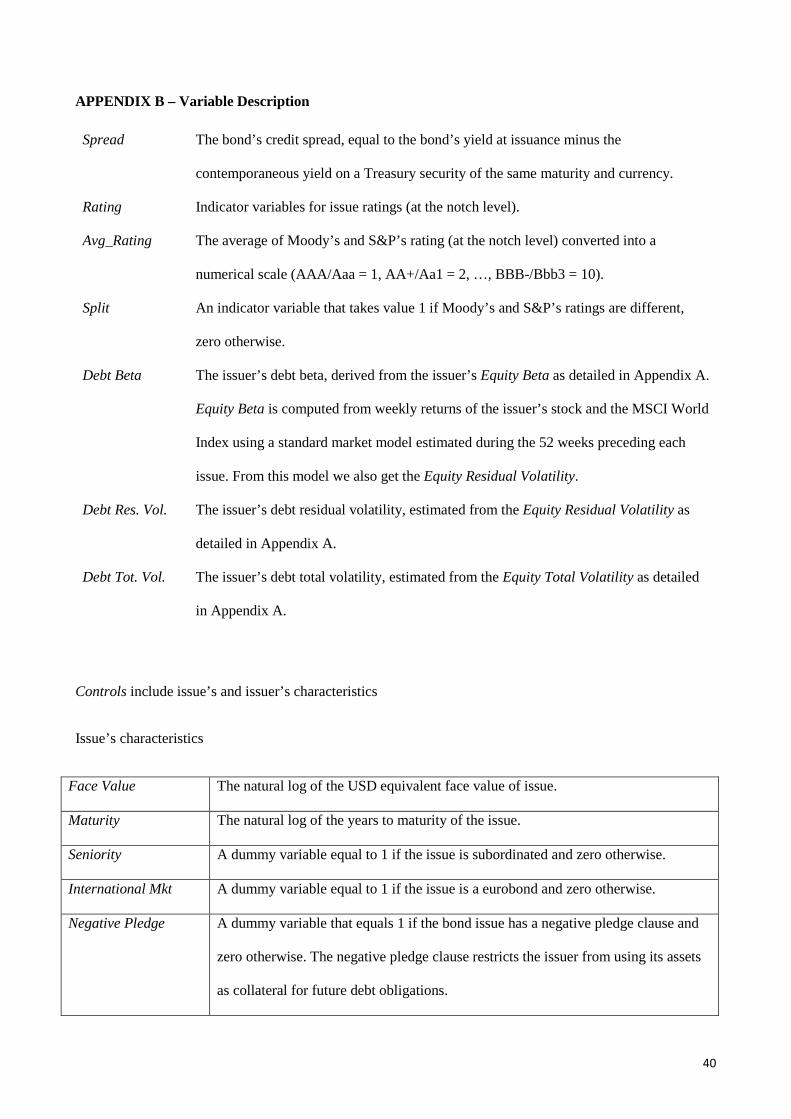
APPENDIX B – Variable Description

Spread The bond’s credit spread, equal to the bond’s yield at issuance minus the

contemporaneous yield on a Treasury security of the same maturity and currency.

Rating Indicator variables for issue ratings (at the notch level).

Avg_Rating The average of Moody’s and S&P’s rating (at the notch level) converted into a

numerical scale (AAA/Aaa = 1, AA+/Aa1 = 2, …, BBB-/Bbb3 = 10).

Split An indicator variable that takes value 1 if Moody’s and S&P’s ratings are different,

zero otherwise.

Debt Beta The issuer’s debt beta, derived from the issuer’s Equity Beta as detailed in Appendix A.

Equity Beta is computed from weekly returns of the issuer’s stock and the MSCI World

Index using a standard market model estimated during the 52 weeks preceding each

issue. From this model we also get the Equity Residual Volatility.

Debt Res. Vol. The issuer’s debt residual volatility, estimated from the Equity Residual Volatility as

detailed in Appendix A.

Debt Tot. Vol. The issuer’s debt total volatility, estimated from the Equity Total Volatility as detailed

in Appendix A.

Controls include issue’s and issuer’s characteristics

Issue’s characteristics

Face Value The natural log of the USD equivalent face value of issue.

Maturity The natural log of the years to maturity of the issue.

Seniority A dummy variable equal to 1 if the issue is subordinated and zero otherwise.

International Mkt A dummy variable equal to 1 if the issue is a eurobond and zero otherwise.

Negative Pledge A dummy variable that equals 1 if the bond issue has a negative pledge clause and

zero otherwise. The negative pledge clause restricts the issuer from using its assets

as collateral for future debt obligations.

40

Reg D A dummy variable equal to 1 if the issue is Regulation D and zero otherwise.

Reg S A dummy variable equal to 1 if the issue is Regulation S and zero otherwise.

Rule 144a A dummy variable equal to 1 if the issue is Rule 144a and zero otherwise.

Fungible A dummy variable equal to 1 if the issue is fungible and zero otherwise.

Force majeure A dummy variable equal to 1 if the issue has a force majeure clause and zero

otherwise.

Shelf registration A dummy variable equal to 1 if the issue is shelf-registered and zero otherwise.

Cross-default A dummy variable that equals 1 if the bond issue has a cross-default clause and zero

otherwise. The cross-default clause avoids the possibility of selective default on the

part of the issuer. If the issuer is insolvent on one loan or bond issue, it is

automatically considered as insolvent on all other loans and obligations.

Year Year fixed effects.

Currency Currency fixed effects.

Avg Bid-Ask Spread The average bid-ask spread over the 60 trading days following the issuance of each

bond. This variable is available for 2,395 bonds (out of the entire sample of 3,924

bonds).

Issuer’s characteristics

Size The natural log of the USD equivalent issuer’s market capitalization.

Country Country fixed effects.

Industry Industry fixed effects.

41

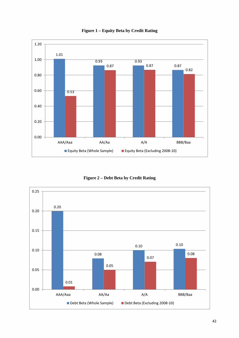
Figure 1 – Equity Beta by Credit Rating

Figure 2 – Debt Beta by Credit Rating

1.01

0.93 0.93 0.87

0.53

0.87 0.87 0.82

0.00

0.20

0.40

0.60

0.80

1.00

1.20

AAA/Aaa AA/Aa A/A BBB/Baa

Equity Beta (Whole Sample) Equity Beta (Excluding 2008-10)

0.20

0.08

0.10 0.10

0.01

0.05

0.07 0.08

0.00

0.05

0.10

0.15

0.20

0.25

AAA/Aaa AA/Aa A/A BBB/Baa

Debt Beta (Whole Sample) Debt Beta (Excluding 2008-10)

42

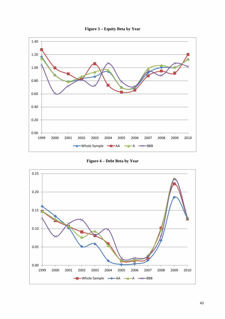
Figure 3 – Equity Beta by Year

Figure 4 – Debt Beta by Year

0.00

0.20

0.40

0.60

0.80

1.00

1.20

1.40

1999 2000 2001 2002 2003 2004 2005 2006 2007 2008 2009 2010

Whole Sample AA A BBB

0.00

0.05

0.10

0.15

0.20

0.25

1999 2000 2001 2002 2003 2004 2005 2006 2007 2008 2009 2010

Whole Sample AA A BBB

43

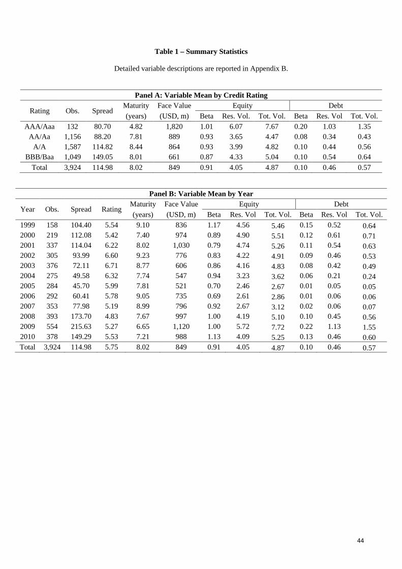
Table 1 – Summary Statistics

Detailed variable descriptions are reported in Appendix B.

Panel A: Variable Mean by Credit Rating

Rating Obs. Spread Maturity Face Value Equity Debt (years) (USD, m) Beta Res. Vol. Tot. Vol. Beta Res. Vol Tot. Vol.

AAA/Aaa 132 80.70 4.82 1,820 1.01 6.07 7.67 0.20 1.03 1.35 AA/Aa 1,156 88.20 7.81 889 0.93 3.65 4.47 0.08 0.34 0.43

A/A 1,587 114.82 8.44 864 0.93 3.99 4.82 0.10 0.44 0.56 BBB/Baa 1,049 149.05 8.01 661 0.87 4.33 5.04 0.10 0.54 0.64

Total 3,924 114.98 8.02 849 0.91 4.05 4.87 0.10 0.46 0.57

Panel B: Variable Mean by Year

Year Obs. Spread Rating Maturity Face Value Equity Debt (years) (USD, m) Beta Res. Vol Tot. Vol. Beta Res. Vol Tot. Vol.

1999 158 104.40 5.54 9.10 836 1.17 4.56 5.46 0.15 0.52 0.64 2000 219 112.08 5.42 7.40 974 0.89 4.90 5.51 0.12 0.61 0.71 2001 337 114.04 6.22 8.02 1,030 0.79 4.74 5.26 0.11 0.54 0.63 2002 305 93.99 6.60 9.23 776 0.83 4.22 4.91 0.09 0.46 0.53 2003 376 72.11 6.71 8.77 606 0.86 4.16 4.83 0.08 0.42 0.49 2004 275 49.58 6.32 7.74 547 0.94 3.23 3.62 0.06 0.21 0.24 2005 284 45.70 5.99 7.81 521 0.70 2.46 2.67 0.01 0.05 0.05 2006 292 60.41 5.78 9.05 735 0.69 2.61 2.86 0.01 0.06 0.06 2007 353 77.98 5.19 8.99 796 0.92 2.67 3.12 0.02 0.06 0.07 2008 393 173.70 4.83 7.67 997 1.00 4.19 5.10 0.10 0.45 0.56 2009 554 215.63 5.27 6.65 1,120 1.00 5.72 7.72 0.22 1.13 1.55 2010 378 149.29 5.53 7.21 988 1.13 4.09 5.25 0.13 0.46 0.60 Total 3,924 114.98 5.75 8.02 849 0.91 4.05 4.87 0.10 0.46 0.57

44

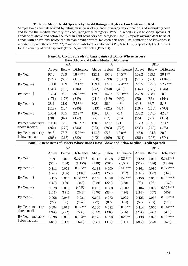
Table 2 – Mean Credit Spreads by Credit Ratings – High vs. Low Systematic Risk Sample bonds are categorized by rating class, year of issuance, currency denomination, and maturity (above and below the median maturity for each rating-year category). Panel A reports average credit spreads of bonds with above and below the median debt betas for each category. Panel B reports average debt betas of bonds with above and below the median credit spreads for each category. The number of observations is reported in parentheses. ***, **, * indicate statistical significance (1%, 5%, 10%, respectively) of the t-test for the equality of credit spreads (Panel A) or debt betas (Panel B).

Panel A: Credit Spreads (in basis points) of Bonds Whose Issuers

Have Above and Below Median Debt Betas AA A BBB

Above Below Difference Above Below Difference Above Below Difference By Year 97.6 78.9 18.7*** 122.1 107.6 14.5*** 159.2 139.1 20.1**

(573) (583) (1,156) (788) (799) (1,587) (518) (531) (1,049) By Year - € 111.0 93.9 17.1** 159.4 127.0 32.4*** 228.5 175.8 52.7***

(146) (158) (304) (242) (250) (492) (167) (179) (346) By Year - $ 132.4 96.1 36.3*** 179.5 147.2 32.3*** 268.9 258.1 10.8

(171) (178) (349) (211) (219) (430) (78) (86) (164) By Year - ¥ 28.4 21.0 7.5*** 30.8 26.0 4.8* 41.8 36.7 5.1*

(112) (134) (246) (213) (221) (434) (197) (206) (403) By Year - £ 106.4 83.5 22.9** 136.3 137.7 -1.4 230.2 187.6 42.5*

(70) (82) (152) (77) (87) (164) (55) (60) (115) By Year –maturity above median

103.6 77.1 26.5*** 128.9 120.8 8.1 177.3 155.9 21.4* (264) (272) (536) (383) (393) (776) (233) (242) (475)

By Year –maturity below median

94.6 78.7 15.9*** 114.8 95.8 19.0** 145.0 124.8 20.2 (305) (315) (620) (402) (409) (811) (281) (293) (574)

Panel B: Debt Betas of Issuers Whose Bonds Have Above and Below Median Credit Spreads AA A BBB

Above Below Difference Above Below Difference Above Below Difference By Year 0.091 0.067 0.024*** 0.113 0.088 0.025*** 0.120 0.087 0.033***

(576) (580) (1,156) (790) (797) (1,587) (519) (530) (1,049) By Year - € 0.111 0.076 0.035** 0.133 0.090 0.042*** 0.161 0.089 0.072***

(148) (156) (304) (242) (250) (492) (169) (177) (346) By Year - $ 0.115 0.075 0.040*** 0.148 0.098 0.050*** 0.150 0.068 0.082***

(169) (180) (349) (209) (221) (430) (78) (86) (164) By Year - ¥ 0.078 0.053 0.025* 0.085 0.088 -0.002 0.104 0.077 0.027***

(115) (131) (246) (200) (234) (434) (196) (207) (403) By Year - £ 0.068 0.046 0.021 0.075 0.072 0.002 0.125 0.057 0.068***

(72) (80) (152) (77) (87) (164) (53) (62) (115) By Year –maturity above median

0.084 0.062 0.022** 0.100 0.082 0.019** 0.114 0.070 0.044*** (264) (272) (536) (382) (394) (776) (234) (241) (475)

By Year –maturity below median

0.096 0.073 0.024** 0.120 0.098 0.022** 0.130 0.098 0.032*** (303) (317) (620) (401) (410) (811) (282) (292) (574)

45

Table 3 – Average Increase in Beta of Bonds with Above Median Credit Spreads

Sample bonds are categorized by year, rating class, currency denomination, and maturity (above and below the median of the year-rating-currency category). For each category with at least 10 issues, we compute the ratio of the average beta of bonds with above median credit spreads to the average beta of all the bonds within that category. This table reports the mean log ratios. ***, **, * indicate statistical significance (1%, 5%, 10%, respectively) of the t-test for the equality of the mean log ratios to zero.

Maturity € $ ¥ Total Below 0.189** 0.212*** 0.005 0.145*** Above 0.137 0.309*** 0.071 0.187*** Total 0.166*** 0.261*** 0.036 0.165***

46

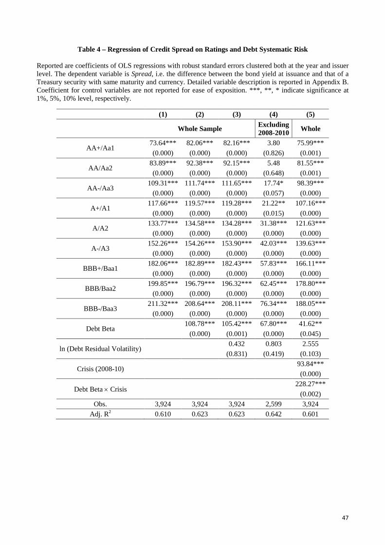
Table 4 – Regression of Credit Spread on Ratings and Debt Systematic Risk

Reported are coefficients of OLS regressions with robust standard errors clustered both at the year and issuer level. The dependent variable is Spread, i.e. the difference between the bond yield at issuance and that of a Treasury security with same maturity and currency. Detailed variable description is reported in Appendix B. Coefficient for control variables are not reported for ease of exposition. ***, **, * indicate significance at 1%, 5%, 10% level, respectively.

(1) (2) (3) (4) (5)

Whole Sample Excluding 2008-2010 Whole

AA+/Aa1 73.64*** 82.06*** 82.16*** 3.80 75.99*** (0.000) (0.000) (0.000) (0.826) (0.001)

AA/Aa2 83.89*** 92.38*** 92.15*** 5.48 81.55*** (0.000) (0.000) (0.000) (0.648) (0.001)

AA-/Aa3 109.31*** 111.74*** 111.65*** 17.74* 98.39***

(0.000) (0.000) (0.000) (0.057) (0.000)

A+/A1 117.66*** 119.57*** 119.28*** 21.22** 107.16***

(0.000) (0.000) (0.000) (0.015) (0.000)

A/A2 133.77*** 134.58*** 134.28*** 31.38*** 121.63***

(0.000) (0.000) (0.000) (0.000) (0.000)

A-/A3 152.26*** 154.26*** 153.90*** 42.03*** 139.63***

(0.000) (0.000) (0.000) (0.000) (0.000)

BBB+/Baa1 182.06*** 182.89*** 182.43*** 57.83*** 166.11***

(0.000) (0.000) (0.000) (0.000) (0.000)

BBB/Baa2 199.85*** 196.79*** 196.32*** 62.45*** 178.80***

(0.000) (0.000) (0.000) (0.000) (0.000)

BBB-/Baa3 211.32*** 208.64*** 208.11*** 76.34*** 188.05***

(0.000) (0.000) (0.000) (0.000) (0.000)

Debt Beta 108.78*** 105.42*** 67.80*** 41.62** (0.000) (0.001) (0.000) (0.045)

ln (Debt Residual Volatility) 0.432 0.803 2.555 (0.831) (0.419) (0.103)

Crisis (2008-10) 93.84*** (0.000)

Debt Beta × Crisis 228.27*** (0.002)

Obs. 3,924 3,924 3,924 2,599 3,924 Adj. R2 0.610 0.623 0.623 0.642 0.601

47

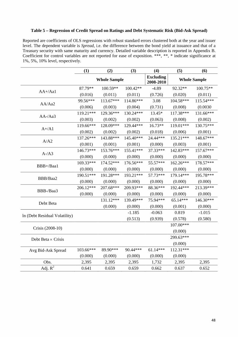
Table 5 – Regression of Credit Spread on Ratings and Debt Systematic Risk (Bid-Ask Spread)

Reported are coefficients of OLS regressions with robust standard errors clustered both at the year and issuer level. The dependent variable is Spread, i.e. the difference between the bond yield at issuance and that of a Treasury security with same maturity and currency. Detailed variable description is reported in Appendix B. Coefficient for control variables are not reported for ease of exposition. ***, **, * indicate significance at 1%, 5%, 10% level, respectively.

(1) (2) (3) (4) (5) (6)

Whole Sample Excluding 2008-2010 Whole Sample

AA+/Aa1 87.79** 100.59** 100.42** -4.89 92.32** 100.75** (0.016) (0.011) (0.011) (0.726) (0.020) (0.011)

AA/Aa2 99.56*** 113.67*** 114.86*** 3.08 104.58*** 115.54*** (0.006) (0.003) (0.004) (0.731) (0.008) (0.0030

AA-/Aa3 119.21*** 129.36*** 130.24*** 13.45* 117.38*** 131.66***

(0.003) (0.002) (0.002) (0.063) (0.008) (0.002)

A+/A1 119.66*** 128.09*** 129.44*** 16.73** 119.01*** 130.75***

(0.002) (0.002) (0.002) (0.018) (0.006) (0.001)

A/A2 137.26*** 143.88*** 145.40*** 24.44*** 135.21*** 148.67***

(0.001) (0.001) (0.001) (0.000) (0.003) (0.001)

A-/A3 146.73*** 153.76*** 155.41*** 37.33*** 142.83*** 157.67***

(0.000) (0.000) (0.000) (0.000) (0.000) (0.000)

BBB+/Baa1 169.33*** 174.52*** 176.56*** 55.57*** 162.26*** 178.57***

(0.000) (0.000) (0.000) (0.000) (0.000) (0.000)

BBB/Baa2 190.51*** 191.28*** 193.21*** 57.73*** 179.14*** 195.78***

(0.000) (0.000) (0.000) (0.000) (0.000) (0.000)

BBB-/Baa3 206.12*** 207.68*** 209.93*** 88.36*** 192.44*** 213.39***

(0.000) (0.000) (0.000) (0.000) (0.000) (0.000)

Debt Beta 131.12*** 139.49*** 75.94*** 65.14*** 146.30*** (0.000) (0.000) (0.000) (0.001) (0.000)

ln (Debt Residual Volatility) -1.185 -0.063 0.819 -1.015 (0.513) (0.939) (0.578) (0.580)

Crisis (2008-10) 107.00*** (0.000)

Debt Beta × Crisis 299.63*** (0.000)

Avg Bid-Ask Spread

103.66*** 89.90*** 90.44*** 61.14*** 112.31*** (0.000) (0.000) (0.000) (0.000) (0.000)

Obs. 2,395 2,395 2,395 1,732 2,395 2,395 Adj. R2 0.641 0.659 0.659 0.662 0.637 0.652

48

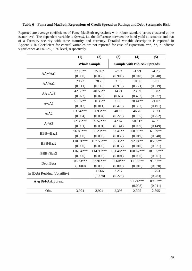
Table 6 – Fama and MacBeth Regressions of Credit Spread on Ratings and Debt Systematic Risk

Reported are average coefficients of Fama-MacBeth regressions with robust standard errors clustered at the issuer level. The dependent variable is Spread, i.e. the difference between the bond yield at issuance and that of a Treasury security with same maturity and currency. Detailed variable description is reported in Appendix B. Coefficient for control variables are not reported for ease of exposition. ***, **, * indicate significance at 1%, 5%, 10% level, respectively.

(1) (2) (3) (4) (5)

Whole Sample Sample with Bid-Ask Spreads

AA+/Aa1 27.10** 25.09* -2.93 -1.59 -4.75 (0.050) (0.055) (0.908) (0.948) (0.848)

AA/Aa2 29.22 28.76 3.15 10.36 3.01

(0.111) (0.118) (0.915) (0.721) (0.919)

AA-/Aa3 42.36** 40.53** 14.71 23.99 15.82 (0.023) (0.026) (0.65) (0.463) (0.627)

A+/A1 51.97** 50.35** 21.16 28.44** 21.07 (0.012) (0.011) (0.479) (0.352) (0.491)

A/A2 63.54*** 61.93*** 40.13 46.76 38.33 (0.004) (0.004) (0.229) (0.165) (0.252)

A-/A3 72.36*** 69.57*** 42.67 50.31* 42.21 (0.001) (0.001) (0.141) (0.089) (0.149)

BBB+/Baa1 96.83*** 95.29*** 63.41** 68.95** 61.09** (0.000) (0.000) (0.033) (0.019) (0.040)

BBB/Baa2 110.01*** 107.53*** 85.35** 92.04** 85.05**

(0.000) (0.000) (0.017) (0.010) (0.021)

BBB-/Baa3 116.84*** 114.90*** 101.48*** 108.87*** 101.55***

(0.000) (0.000) (0.001) (0.000) (0.001)

Debt Beta 106.23*** 82.91*** 92.60*** 111.58** 91.67**

(0.000) (0.000) (0.006) (0.016) (0.020)

ln (Debt Residual Volatility) 1.566 2.217 1.753 (0.378) (0.225) (0.283)

Avg Bid-Ask Spread

91.24*** 89.97** (0.008) (0.011)

Obs. 3,924 3,924 2,395 2,395 2,395

49

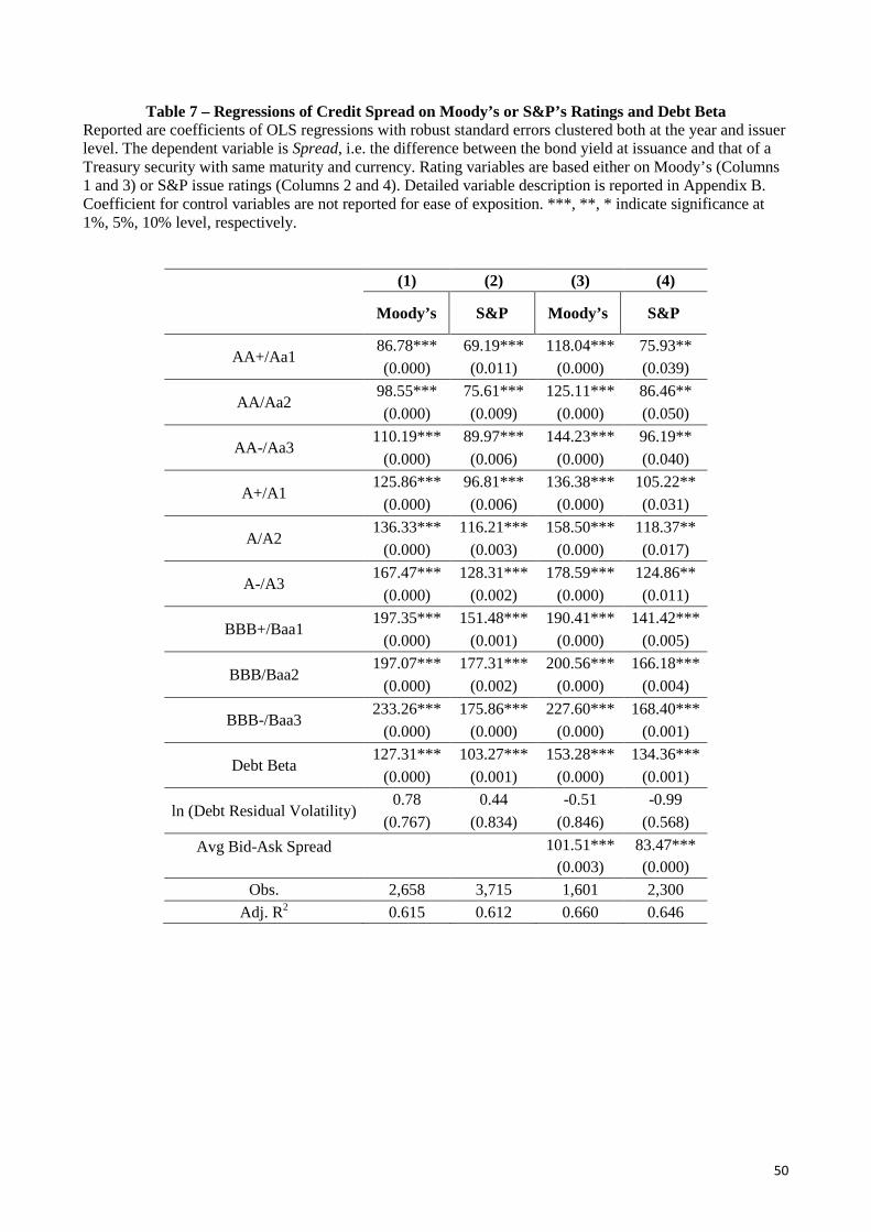
Table 7 – Regressions of Credit Spread on Moody’s or S&P’s Ratings and Debt Beta Reported are coefficients of OLS regressions with robust standard errors clustered both at the year and issuer level. The dependent variable is Spread, i.e. the difference between the bond yield at issuance and that of a Treasury security with same maturity and currency. Rating variables are based either on Moody’s (Columns 1 and 3) or S&P issue ratings (Columns 2 and 4). Detailed variable description is reported in Appendix B. Coefficient for control variables are not reported for ease of exposition. ***, **, * indicate significance at 1%, 5%, 10% level, respectively.

(1) (2) (3) (4)

Moody’s S&P Moody’s S&P

AA+/Aa1 86.78*** 69.19*** 118.04*** 75.93** (0.000) (0.011) (0.000) (0.039)

AA/Aa2 98.55*** 75.61*** 125.11*** 86.46** (0.000) (0.009) (0.000) (0.050)

AA-/Aa3 110.19*** 89.97*** 144.23*** 96.19**

(0.000) (0.006) (0.000) (0.040)

A+/A1 125.86*** 96.81*** 136.38*** 105.22**

(0.000) (0.006) (0.000) (0.031)

A/A2 136.33*** 116.21*** 158.50*** 118.37**

(0.000) (0.003) (0.000) (0.017)

A-/A3 167.47*** 128.31*** 178.59*** 124.86**

(0.000) (0.002) (0.000) (0.011)

BBB+/Baa1 197.35*** 151.48*** 190.41*** 141.42***

(0.000) (0.001) (0.000) (0.005)

BBB/Baa2 197.07*** 177.31*** 200.56*** 166.18***

(0.000) (0.002) (0.000) (0.004)

BBB-/Baa3 233.26*** 175.86*** 227.60*** 168.40***

(0.000) (0.000) (0.000) (0.001)

Debt Beta 127.31*** 103.27*** 153.28*** 134.36***

(0.000) (0.001) (0.000) (0.001)

ln (Debt Residual Volatility) 0.78 0.44 -0.51 -0.99

(0.767) (0.834) (0.846) (0.568) Avg Bid-Ask Spread

101.51*** 83.47*** (0.003) (0.000)

Obs. 2,658 3,715 1,601 2,300 Adj. R2 0.615 0.612 0.660 0.646

50

Table 8 – Regressions of Ratings on Debt Systematic Risk

In Panel A are reported coefficients of OLS regressions (Columns 1-6) and ordered probit (Columns 7-8) with robust standard errors clustered both at the year and issuer level. The dependent variable is Avg_Rating, i.e. the average of Moody’s and S&P’s issue ratings, converted into numerical scale (AAA/Aaa = 1, AA-/Aa1 = 2, …, BBB-/Bbb3 = 10). In Panel B are reported coefficients of OLS regressions with robust standard errors clustered both at the year and issuer level. The dependent variable is Rating that is either Moody’s or S&P’s issue rating, converted into numerical scale (AAA/Aaa = 1, AA-/Aa1 = 2, …, BBB-/Bbb3 = 10). Detailed variable description is reported in Appendix B. Coefficient for control variables are not reported for ease of exposition. ***, **, * indicate significance at 1%, 5%, 10% level, respectively.

Panel A: Regressions of Average Ratings on Debt Systematic Risk

(1) (2) (3) (4) (5) (6) (7) (8)

OLS Ordered Probit Whole Sample Excluding 2008-2010

Debt Beta 1.875*** 0.917 0.883 2.947*** 1.682*** 1.627*** 1.259*** 1.219*** (0.006) (0.202) (0.218) (0.000) (0.002) (0.003) (0.000) (0.000)

ln (Debt Residual Volatility) 0.123*** 0.155*** 0.109*** (0.000) (0.000) (0.000)

ln (Debt Total Volatility) 0.121*** 0.153*** 0.108*** (0.000) (0.000) (0.000)

Obs. 3,924 3,924 3,924 2,599 2,599 2,599 2,599 2,599 Adj. R2 0.474 0.482 0.481 0.523 0.537 0.537 0.186 0.186

Panel B: Regressions of Moody’s Rating or S&P’s Rating on Debt Systematic Risk

(1) (2) (3) (4) (5) (6) (7) (8)

Whole Sample Excluding 2008-2010 Moody's S&P's Moody's S&P's

Debt Beta 0.664 0.631 0.553 0.527 1.527*** 1.451*** 1.441*** 1.391**

(0.494) (0.516) (0.472) (0.493) (0.002) (0.005) (0.008) (0.012) ln (Debt Residual

Volatility) 0.136*** 0.128*** 0.190*** 0.160*** (0.002) (0.000) (0.000) (0.000)

ln (Debt Total Volatility)

0.134*** 0.126*** 0.188*** 0.158*** (0.002) (0.000) (0.000) (0.000)

Obs. 2,658 2,658 3,715 3,715 1,472 1,472 2,489 2,489 Adj. R2 0.523 0.523 0.475 0.475 0.564 0.564 0.538 0.538

51