Banking Efficiency, Risk and Stock Performance in the ... · Banking Efficiency, Risk and Stock...

Banking Efficiency, Risk and Stock Performance in

the European Union Banking System: the Effect of the

World Financial Crisis

Thesis submitted for the degree of

Doctor of Philosophy

at the University of Leicester

By

Saleem Janoudi

School of Management

University of Leicester

2014

ii

Banking Efficiency, Risk and Stock Performance in

the European Union Banking System: the Effect of the


By Saleem Janoudi

Abstract

This thesis has three main objectives; first, it assesses and evaluates cost and profit

efficiencies of the European Union banking system by employing the stochastic

frontier analysis (SFA) over the period 2004-2010. It divides the EU region into four

groups; the entire EU region, the old and the new EU countries as well as the GIIPS

countries. Second, this study investigates the determinants of bank cost and profit

inefficiencies with the focus mainly being on the role of banking risks and the world

financial crisis (2007-2009) in affecting banking efficiency. Third, this thesis evaluates

the impact of different variables on bank stock returns, with the emphasis on bank

efficiency, risk and the world financial crisis, over the period 2004-2010.

The empirical findings show that commercial banks in the EU improve their cost and

profit efficiencies on average between 2004 and 2010. Also, banks in the old EU

countries appear to be more cost efficient but less profit efficient compared to banks in

the new EU countries. Interestingly, the empirical analysis concludes that overall

insolvency, credit and liquidity risks have significant and positive effects on bank cost

and profit inefficiencies during the world financial crisis, suggesting that banks that

maintain less risk outperform their counterparts during crisis time. The world financial

crisis appears to affect negatively both cost and profit efficiencies of EU banks;

however, it has stronger negative effect on banks in the old EU member states than in

the new EU countries. Finally, the results show that changes in cost and profit

efficiencies along with capital and size variables appear to have a positive and

significant influence on bank stock performance in the EU and that bank stock returns

are significantly sensitive to market and interest rate risks.

iii

Acknowledgements

I would like to express my gratitude to my respected supervisors, Professor Peter

Jackson and Dr Mohamed Shaban, for their advice and guidance in writing this thesis.

I have greatly benefited from their comments and constructive criticisms which have

significantly improved the purpose and the content of this thesis. Also, they patiently

provided the vision, encouragement and advice necessary for me to successfully

proceed through the doctorial program and complete my thesis. My heartfelt

appreciation goes to my parents for their unconditional love and endless support

throughout the process of writing this thesis. They have spent their lives paving the

way to highly educate me in order for me to become a successful and notable person in

this life. I am, also, in debt to my brothers and sisters for their inspiring support and

precious encouragement over the years of conducting this thesis. Last but not least, I

want to thank all my friends that I have met during my life in England, in particular

Dogus Emin, with whom, together, we have overcome the hardships of writing our

theses.

This thesis is dedicated to my parents

for their love, endless support

and encouragement

iv

Table of Contents

Abstract ............................................................................................................................ ii

Acknowledgements ........................................................................................................ iii

Table of Contents ........................................................................................................... iv

List of Tables ................................................................................................................ viii

List of Figures ................................................................................................................. ix

List of Acronyms ............................................................................................................. x

1 Background, Objectives, Methodology and Structure of the

Study ...................................................................................................... 1

1.1 Introduction .............................................................................................................. 1

1.2 Objectives and Motivations ..................................................................................... 3

1.3 Research Methodology and Data ............................................................................. 4

1.4 Structure of the Study .............................................................................................. 6

2 Efficiency, Risk and Global Financial Crisis: Theory and

Measurement ........................................................................................ 9

2.1 Introduction .............................................................................................................. 9

2.2 Conventional Versus Frontier Efficiency Methods ............................................... 10

2.3 The Framework of Efficiency ................................................................................ 12

2.3.1 Technical, Allocative, Cost and Revenue Efficiency .............................................. 12

2.3.2 Pure Technical and Scale Efficiency ....................................................................... 16

2.3.3 Economies of Scale and Scope ................................................................................ 18

2.4 The Measurement of Efficiency ............................................................................. 20

2.4.1 Data Envelopment Analysis (DEA) ........................................................................ 20

2.4.2 Free Disposal Hull (FDH) ....................................................................................... 21

2.4.3 Stochastic Frontier Analysis (SFA) ......................................................................... 21

2.4.4 Distribution Free Approach (DFA) ......................................................................... 22

2.4.5 Thick Frontier Approach (TFA) .............................................................................. 23

2.4.6 What is the Best Frontier Method?.......................................................................... 24

2.5 Risk in Banking Institutions ................................................................................... 25

2.5.1 Banking Risks Overview and CAPM ...................................................................... 26

2.5.2 Insolvency Risk ....................................................................................................... 27

2.5.3 Credit Risk............................................................................................................... 28

2.5.4 Liquidity Risk .......................................................................................................... 29

2.5.5 Market (or Trading) Risk ........................................................................................ 30

v

2.5.6 Capital Requirements and Bank Risks .................................................................... 30

2.6 World Financial Crisis ........................................................................................... 32

2.6.1 Overview of the World Financial Crisis .................................................................. 32

2.6.2 World Financial Crisis and Banking Risks ............................................................. 35

2.7 Eurozone Debt Crisis ............................................................................................. 38

2.8 Summary and Conclusion ...................................................................................... 40

3 The Structure and Regulatory Environment in the EU Banking

System and Selected Literature on Banking Efficiency and

Risk ...................................................................................................... 42

3.1 Introduction ............................................................................................................ 42

3.2 The European Union Banking System: Regulation and Structure ......................... 43

3.2.1 Deregulation and Re-regulation in European Banking Markets ............................. 43

3.2.2 European Monetary Union and the Adoption of the Euro ...................................... 46

3.2.3 European Banking Structure ................................................................................... 47

3.2.4 The Eastern Enlargement of the European Union ................................................... 54

3.3 Literature Review on European Banking Efficiency ............................................. 56

3.3.1 Comparative Efficiency Studies in the EU Banking Markets ................................. 57

3.3.2 Bank Efficiency, Integration, Ownership and Consolidation .................................. 63

3.4 Literature on Risk in European Banking ............................................................... 66

3.4.1 Bank Efficiency and Risk ........................................................................................ 67

3.4.2 Banking Risk in the EU ........................................................................................... 69

3.5 Summary and Conclusion ...................................................................................... 72

4 Methodology and Data ...................................................................... 74

4.1 Introduction ............................................................................................................ 74

4.2 Measuring Banking Efficiency .............................................................................. 75

4.2.1 Stochastic Frontier Analysis (SFA) ......................................................................... 75

4.2.2 Stochastic Frontier Models for Panel Data .............................................................. 76

4.2.2.1 Panel Data Cost Frontier Models and Specification.................................. 78

4.2.2.2 Panel Data Profit Frontier Models and Specification ................................ 85

4.3 Measuring Banking Risk ........................................................................................ 88

4.4 Data Description and Variables ............................................................................. 90

4.4.1 Bank Efficiency and its Determinants ..................................................................... 90

4.4.1.1 The Input and Output Variables (Control Variables) ................................ 92

4.4.1.2 The Environmental Variables (Efficiency Correlates) .............................. 95

4.5 Summary and Conclusion .................................................................................... 105

vi

5 Empirical Analysis of Efficiency in the European Union Banking

Sector ................................................................................................. 106

5.1 Introduction .......................................................................................................... 106

5.2 Efficiency Frontier Estimates .............................................................................. 107

5.2.1 Cost Frontier Estimates ......................................................................................... 107

5.2.2 Profit Frontier Estimates ....................................................................................... 110

5.3 Bank Efficiency Levels ........................................................................................ 113

5.3.1 Cost Efficiency Levels .......................................................................................... 113

5.3.2 Profit Efficiency Levels ........................................................................................ 117

5.3.3 Cost and Profit Efficiency Levels and Bank Size ................................................. 121

5.4 Bank Efficiency Evolution ................................................................................... 123

5.5 Dispersion of Bank Efficiency ............................................................................. 127

5.6 Global Financial Crisis and Efficiency ................................................................ 129


6 Risk and Determinants of Efficiency in the European Union

Banking Sector ................................................................................. 136

6.1 Introduction .......................................................................................................... 136

6.2 Bank Risk Analysis .............................................................................................. 137

6.3 Risk, Cost and Profit Inefficiencies: Determinants of Cost and Profit

Inefficiencies (Environmental Variables) ............................................................ 144

6.3.1 Bank Risk Effects on Inefficiency......................................................................... 148

6.3.2 Other Variables’ Effects on Inefficiency ............................................................... 153

6.4 Rank Order Correlation of Efficiency Scores and Traditional Non-Frontier

Performance Measures ......................................................................................... 161


7 Bank Stock Performance, Efficiency and Risk in the European

Union Market ................................................................................... 166

7.1 Introduction .......................................................................................................... 166

7.2 Literature Review ................................................................................................. 168

7.2.1 Studies on Bank Efficiency and Stock Performance ............................................. 168

7.2.2 Studies on Risk and Stock Performance ................................................................ 172

7.3 Methodology and Data ......................................................................................... 175

7.3.1 Measuring Bank Stock Return and its Determinants ................................ 175

7.3.1.1 Panel Data Estimation Methods ............................................................. 175

7.3.1.2 The Regression Models’ Specification ................................................... 177

7.3.1.3 Diagnostic Tests ..................................................................................... 179

vii

7.3.2 Variables Specification and Definition ..................................................... 181

7.4 Empirical Results: Analysis and Discussion ........................................................ 191

7.4.1 Model (A) Regression Results .............................................................................. 191

7.4.2 Model (B) Regression Results ............................................................................... 197


8 Conclusions and Limitations of the Research ............................... 202

8.1 Introduction and Summary of Findings ............................................................... 202

8.2 Policy Implications .............................................................................................. 205

8.3 Limitations of the Study and Future Research ..................................................... 207

Appendices ............................................................................................... 210

Appendix 1: Cross-Sectional Cost Frontier Models ..................................................... 210

Appendix 2a: Number of Banks and Observations in sample for Countries ................ 212

Appendix 2b: Expected Signs of the Determinants of Banks’ Inefficiency ................. 213

Appendix 2c: Descriptive Statistics of the Determinants of Banks’ Inefficiency ........ 214

Appendix 3: Cost and Profit Efficiency Estimates and Evolution for EU Groups ................ 215

Appendix 4: Correlation Matrix of Environmental Variables ...................................... 216

Appendix 5a: Number of Banks and Observations in Sample for Countries ............... 218

Appendix 5b: Descriptive Statistics and Trends of Cost/Income and ROE Ratios ................ 219

Appendix 5c: Expected Signs of the Determinants of Bank Stock Return ................... 220

Appendix 5d: Stock Returns Correlation ...................................................................... 220

Appendix 6a: Model (A) Regression Diagnostic Tests of STATA for Model (I) ........ 221

Appendix 6b: Model (A) Regression Diagnostic Tests of STATA for Model (II) ...... 222

Appendix 6c: Model (A) Regression Diagnostic Tests of STATA for Model (III) ..... 224

Appendix 6d: Model (A) Regression Diagnostic Tests of STATA for Model (IV) ..... 225

Appendix 6e: Model (B) Regression Diagnostic Tests of STATA .............................. 227

Bibliography ............................................................................................. 229

viii

List of Tables

Table 3.1 Structural Financial Indicators for the EU15 Banking Sectors .................... 50

Table 3.2 Structural Financial Indicators for the EU12 Banking Sectors .................... 51

Table 4.1 Input and Output Variables .......................................................................... 93

Table 4.2 Descriptive Statistics of Dependent variables, Input Prices and Outputs .... 95

Table 5.1 Maximum Likelihood Estimates for Cost Function Models ..................... 108

Table 5.2 Maximum Likelihood Estimates for Profit Function Models .................... 111

Table 5.3 Cost Efficiency Estimates: Common vs. Separate Frontiers ..................... 114

Table 5.4 Cost Efficiency Estimates and Evolution .................................................. 117

Table 5.5 Profit Efficiency Estimates: Common vs. Separate Frontier ..................... 119

Table 5.6 Profit Efficiency Estimates and Evolution ................................................. 121

Table 5.7 Average Cost and Profit Efficiencies by size Groups ................................ 122

Table 5.8 Cost Efficiency Estimates and Crisis ......................................................... 130

Table 5.9 Profit Efficiency Estimates and Crisis ....................................................... 132

Table 6.1 Bank Risk Descriptive Statistics for the EU27 and the EUGIIPS ............. 138

Table 6.2 Bank Risk Descriptive Statistics for the EU15 and the EU12 ................... 139

Table 6.3 Determinants of Cost Inefficiency ............................................................. 146

Table 6.4 Determinants of Profit Inefficiency ........................................................... 147

Table 6.5 Spearman’s Rank Correlation of Efficiency and Traditional Performance

Measures .................................................................................................... 163

Table 7.1 Descriptive Statistics of Bank Stock Returns and Risk Factors ................ 189

Table 7.2 Determinants of Stock Returns (Model 1) ................................................. 193

Table 7.3 Determinants of Stock Returns (Model 2) ................................................. 198

ix

List of Figures

Figure 2.1 Farrell’s Efficiency Measures (input-oriented) .......................................... 13

Figure 2.2 Farrell’s Efficiency Measures (output-oriented) ........................................ 15

Figure 2.3 Pure Technical and Scale Efficiency .......................................................... 17

Figure 2.4 Economies and Diseconomies of Scale ...................................................... 19

Figure 3.1 Structural Banking Indicators in the EU (2004-2010) ............................... 53

Figure 5.1 Cost Efficiency Estimates of the EU Banks (2004-2010) ........................ 124

Figure 5.2 Profit Efficiency Estimates of the EU Banks (2004-2010) ...................... 126

Figure 5.3 Dispersion of Bank Cost Efficiency (2004-2010) .................................... 128

Figure 5.4 Dispersion of Bank Profit Efficiency (2004-2010) .................................. 129

Figure 5.5 Bank Cost Efficiency and the Financial Crisis ......................................... 131

Figure 5.6 Bank Profit Efficiency and the Financial Crisis ....................................... 133

Figure 6.1 Equity to Total Assets Ratio (Insolvency Risk) ....................................... 141

Figure 6.2 Total Loans to Total Assets Ratio (Liquidity Risk) ................................. 142

Figure 6.3 Non-Performing Loans to Total Loans Ratio (Credit Risk) ..................... 144

Figure 7.1 Stock Returns of Banks and Market Indices ............................................ 190

x

List of Acronyms

EMU Economic and Monetary Union

ECB European Central Bank

EU European Union

SFA Stochastic Frontier Analysis

DEA Data Envelopment Analysis

REM Random Effects Model

FEM Fixed Effects Model

IMF International Monetary Fund

FDH Free Disposal Hull

DFA Distribution Free Approach

TFA Thick Frontier Approach

CAPM Capital Asset Pricing Model

ROA Return on Assets

ROE Return on Equity

CRS Constant Returns to Scale

VRS Variable Returns to Scale

TE Technical Efficiency

AE Allocative Efficiency

CE Cost Efficiency

PTE Pure Technical Efficiency

SE Scale Efficiency

PE Profit Efficiency

DMU Decision Making Unit

EFA Economic Frontier Approach

ML Maximum Likelihood

OLS Ordinary Least Squares

GLS Generalised Least Squares

xi

VAR Value-at-Risk

CDO Collateralised Debt Obligation

MBS Mortgage-Backed Security

GDP Gross Domestic Product

SEM Single European Market

EMS European Monetary System

EMI European Monetary Institute

ERM Exchange Rate Mechanism

M&A Merger and Acquisition

ECSC European Coal and Steel Community

EEC European Economic Community

EAEC European Atomic Energy Community

EC European Communities

CEE Central and Eastern Europe

SEE South Eastern Europe

CIS Commonwealth of Independent States

ABS Asset-Backed Security

LSDV Least Squares Dummy Variable

MLE Maximum Likelihood Estimation

ROAA Return on Average Assets

APT Arbitrage Pricing Theory

CASR Cumulative Annual Stock Return

ECM Error Component Model

BLUE Best Linear Unbiased Estimator

CLRM Classical Linear Regression Model

VIF Variance-Inflation Factor

LM Lagrange Multiplier

1

Chapter 1

Background, Objectives, Methodology and Structure of the

Study

1.1 Introduction

During the last two decades the integration process has been accelerated in the

European banking markets. The multiple forces of financial deregulation, the

foundation of the Economic and Monetary Union (EMU) and the introduction of the

euro have contributed to that integration. Along with deregulation, the technological

change has contributed to the progressive process of integration and increased

competition in the banking industry (European Central Bank [ECB], 2010b).

Therefore, policy makers and central banks in Europe find it important to study the

impact of these changes on banks’ performance. The performance in terms of cost

reduction or profit maximisation is not the only concern by policy makers and

emphasis has been placed on measuring the risk taken to generate acceptable returns

within a highly competitive banking environment. The improvement in banking

performance also tends to send positive signals to shareholders and investors regarding

the future of the bank in which they invest. This in turn highlights the importance of

measuring how banks’ performance would reflect on banks’ stock performance and

their wealth maximisation objective. It is expected that banks’ managers should aim at

improving bank efficiency, controlling risks and maximising shareholders’ wealth as

long as there is no agency problem.

The financial integration, globalisation, complications of the financial markets and

financial innovation are all reasons that have raised concerns about risk in banking

systems all around the world. Controlling and monitoring banking risks has been an

important issue in recent years because of the negative consequences that risk might

bear towards bank performance. Systematic and unsystematic risk might have a

significant influence on banking performance and indeed on shareholders’ wealth,

which as a result should be taken into consideration when analysing banks’

performance. The recent global financial crisis (2007-2009) has highlighted the

2

importance of maintaining a sound and healthy banking system by monitoring its

performance and risks so as to maintain financial and economic stability. The crisis

has deteriorated the performance of banking and financial markets in the US and

Europe and other regions across the world.

The banking systems of the European Union (EU) member states; the old and the new

states, have faced significant challenges with regard to financial regulations (Casu et

al., 2006). A) Regarding the old EU countries, the Second European Banking

Directive and the single European Passport played a key role in deregulation and

eliminating market entry barriers between those countries. This resulted in a higher

level of competition and a more unified banking market. The combined effects of the

euro introduction, information technology advancement, and the benefitting of new

investors from a global capital market fostered the competition and consolidation in

the European banking system. B) The new EU countries, on the other hand, underwent

major reforms and transformation during the 1990s. They had to move from the

centralised planned economic system and mono-banking system towards more

liberalised financial and banking systems. The banking sectors in these countries have

become more developed due to the flow of foreign capital, market integration, and the

establishment of an efficient regulatory framework (Hollo and Nagy, 2006). While the

accession of the new EU countries creates more opportunities, it also imposes

challenges regarding catching up with the old developed European countries

(Mamatzakis et al., 2008). The characteristics of the new countries’ financial systems

indeed differ from the old ones. The new countries depend heavily on bank finance,

maintain lower levels of financial intermediation, present higher levels of bank

concentration and exhibit higher degrees of foreign involvement in the banking sector

than the old EU states (ECB, 2005). The changes in the structure of the economic and

financial systems of the EU countries are likely to have significant effects on the

performance of banks in this region. So it is interesting to investigate how the

integration and unification between the financial systems in all the EU member states

have influenced the integration in the banking performance, particularly between the

old and the new EU countries.

3

1.2 Objectives and Motivations

This thesis aims to assess and evaluate the performance of European Union

commercial banks in terms of cost and profit efficiencies during the period from 2004

to 2010. This period is of specific importance as it demonstrates a post-transition

period for the new EU countries and the effect of unification and integration of the

banking and financial systems between the newly joined countries to the EU and the

old ones. This represents an interesting case study to analyse and compare between the

performance of banking systems of the old and the new EU member states. In

particular, unveiling to what extent the banking systems in the two groups (old and

new EU countries) are integrated, and how this has influenced the performance of the

banks operating in these countries is an interesting issue to study.

This study clusters the EU countries into four groups and examines banks’ efficiency

in these groups; the entire EU countries (27 countries), the old EU countries (15

countries), the new EU countries (12 countries) and the GIIPS1 countries (5 countries).

We avoid clustering the sample into eurozone and non-eurozone countries as such

comparison is out of the scope of this thesis. The influence of risk factors and the

global financial crisis (2007-2009) as well as other variables on the EU banking

efficiency are also investigated in this study. The study further evaluates the impact of

banks’ efficiency, risk and other variables on banks’ stock returns over the period

2004-2010. The main research questions of this study can be summarised as follows:

1- How do cost and profit efficiency levels of the EU banking system change

during the period 2004-2010?

2- How do bank risks and other environmental variables affect bank cost and

profit inefficiencies?

3- Do variations in banking efficiency and risks explain variations in the EU bank

stock returns over the period from 2004 to 2010?

The contribution of this study to the literature is four-fold. First, to the best of the

author’s knowledge, this is the first study to cover bank cost and profit efficiencies for

1 GIIPS refers to five EU countries that have faced sovereign-debt crisis; Greece, Ireland, Italy, Portugal

and Spain.

4

the entire EU that includes 27 countries while dividing this sample into four groups;

the entire EU, the old EU countries, the new EU countries and the GIIPS countries,

and making comparisons between these groups. This comparison takes place in the

period that follows the joining of ten countries to the EU in 2004 after they

experienced financial transition process. This allows investigation into whether such

countries experience deterioration in their banking efficiency as the pressure of

meeting the criteria for joining the EU is relieved after that year. We investigate both

cost and profit efficiencies because cost efficiency alone might not provide a full

picture regarding bank’s management performance in competitive markets. Some

studies, such as Altunbas et al. (2001) and Maudos et al. (2002a), argue that the

ongoing deregulation and increased competition from non-bank financial

intermediaries postulates not only improving cost efficiency but also profit efficiency.

However, improving efficiency may motivate excessive risk-taking in order to defend

market shares (Koetter and Porath, 2007). Second, this study uses three types of

banking risks that had significant effects in the occurrence of the financial crisis, and

investigates whether the level of these risks at banks matters during the crisis period

(2007-2009) in terms of bank efficiency. Third, this study investigates in what way the

financial crisis affects bank cost and profit efficiencies in the four EU groups and

whether one group is affected more by the crisis than the others. Finally, this study

contributes to the European bank efficiency literature by relating banking efficiency

and risks to banking stock performance in the EU using the largest number of the EU

countries, to the best of our knowledge. The unique experience of the European Union

and the related financial and banking integration between its member states is worthy

of study for many years to come.

1.3 Research Methodology and Data

The stochastic frontier analysis (SFA), as a parametric approach, and the data

envelopment analysis (DEA), as a non-parametric approach, are the most widely used

efficiency frontier methods in the literature (Berger and Humphrey, 1997). Data

envelopment analysis is a linear mathematical programming technique and its

advantage is that it is simple to apply because no functional forms and preliminary

restrictive assumptions are needed, and it performs well with a small sample of firms.

5

However, the main disadvantage of the DEA is that it does not account for random

errors, and therefore it might overestimate the inefficiency term [Berger and

Humphrey (1997) and Coelli et al. (2005)]. On the other hand, the SFA is a stochastic

approach that uses econometric tools to estimate efficiency frontier. The main

advantage of the SFA is that, contrary to the DEA, it allows for random error by using

a composed error model where inefficiency follows an asymmetric distribution and

random error follows a symmetric distribution. Therefore, the SFA provides the

technique by which the inefficiency term can be disentangled from the error term,

resulting in an unbiased estimation of inefficiency differences that are under the

control of banks’ management and independent of exogenous factors [Berger and

Humphrey (1997) and Hollo and Nagy (2006)].

In this thesis the stochastic frontier approach (SFA) is adopted to measure bank

efficiency for the advantage aforementioned. Also, the SFA can account for risk

preference and environmental differences between countries and banks using one stage

analysis which allows for more robust and unbiased efficiency estimates, while DEA

does not allow for that (Weill, 2003). Moreover, as mentioned earlier, the DEA

approach performs better with a small sample which is not the case in this study, hence

the SFA is superior and more suitable to be used in this study. We use the Battese and

Coelli (1995) one-step SFA estimation procedure to generate bank cost and profit

efficiency estimates and investigate their determinants, as opposed to the two-step

model. The two-stage approach has been criticised by Wang and Schmidt (2002) who

argue that the assumption that the inefficiency component is independently and

identically distributed across banks is violated in the second step of the approach,

where the inefficiency estimate is assumed to be dependent on different explanatory

variables.

With regard to investigating the determinants of bank stock return, this study uses

multiple regression models for panel data in which bank stock returns are regressed

against different explanatory variables; such as bank efficiency and risks. The fixed

effects model (FEM) and the random effects model (REM) are the estimation

techniques to be adopted, while the Hausman test is used to choose between the two

estimation techniques. We run different diagnostic tests to investigate problems such

as multicollinearity, heteroskedasticity and autocorrelation and to account for them

where they exist.

6

The thesis uses unbalanced panel dataset, composed of 4250 observations

corresponding to 947 commercial banks operating in the 27 EU states over the period

2004-2010. The number of commercial banks included in the study sample from the

old EU states (745 banks) dominates the number of banks from the new EU states (202

banks). Regarding the GIIPS countries, 202 commercial banks operating in these

countries are included in the sample. The data used to measure bank efficiency and its

determinants are collected from balance sheets and income statements of commercial

banks provided by “Bankscope” database of BVD-IBCA. It is important to mention

here that all listed banks in the EU member states were required to adopt the

International Financial Reporting Standards (IFRS) from 2005 rather than the US

Generally Accepted Accounting Principles (GAAP). Data concerning bank stock

prices are also collected from the “Bankscope” database on a monthly basis.

Macroeconomic data, on the other hand, are collected from the “Datastream” database

developed by Thomson Financial Limited and from the IMF’s International Financial

Statistics.

1.4 Structure of the Study

The structure of this thesis is as follows:

Chapter 2 aims to introduce the theoretical framework regarding productive

efficiency and efficiency measurements, to provide a summary of the types of risk that

can be faced by banks as well as to present summaries of the world financial crisis and

the Eurozone crisis. It briefly discusses the differences between the conventional

methods of measuring performance and the frontier methods of measuring firms’

efficiency. Moreover, it provides a framework of productive efficiency where

technical, allocative, cost and revenue efficiencies are introduced and defined. In

addition, this chapter reviews the main frontier techniques; parametric and non-

parametric, that can be used to measure efficiency. Different types of banking risk and

the relationship between risk and return are also analysed in this chapter. Finally, this

chapter explains briefly the world financial crisis (2007-2009) and its relationship with

banking risks as well as it sheds light briefly on the Eurozone debt crisis.

7

Chapter 3 sheds light on the main changes in European banking structure and

financial regulations that the European Union has gone through in order to create more

unified and stabilised banking systems. It discusses the process of deregulation and re-

regulation in the European banking markets and the related legislative changes since

the late 1970s. Furthermore, this chapter covers briefly the introduction of the

European Monetary Union (EMU) and the adoption of the Euro as well as the stages

and conditions related to them. It also uses five structural banking indicators to explore

and analyse the structure of the EU banking system and the changes associated with it

over the period 2004-2010. Additionally, the Eastern enlargement processes of the EU

together with the transition process through which the accession countries have gone

through, are discussed in this chapter. Moreover, literature review on European

banking efficiency and risk and the relationship between them is reviewed in this

chapter. The main focus in this literature review is on European studies of banking

efficiencies and risks using different measurements and different time periods.

Chapter 4 has the objective of describing and explaining the methodology used to

measure bank efficiency and risk in the EU banking system. It briefly defines the

stochastic frontier analysis (SFA) and the models associated with this frontier method

for panel data. Also, this chapter introduces the SFA translog functional forms for cost

and profit efficiencies and the specifications of such models based on the Battese and

Coelli (1995) one-step procedure. Three financial ratios are defined as the measures to

represent three types of banking risk; insolvency, credit and liquidity risks.

Additionally, Chapter 4 provides dataset description and defines variables for bank

efficiency and its determinants as well as banking risk. This includes efficiency inputs

and outputs and the environmental variables that can be considered as efficiency

correlates.

Chapter 5 provides banking efficiency analysis and empirical results which aim to

investigate and compare cost and profit efficiency levels based on common and

separate frontiers. It introduces cost and profit efficiency mean estimates for the four

EU groups adopted in this study and for the EU countries individually and analyses

efficiency by bank size. This chapter also discusses the evolution and dispersion of

bank cost and profit efficiencies over the seven years under study and provides

comparisons between the country groups, particularly the efficiency gap between the

old and the new EU member states. In this chapter, we also examine the influence of

8

the world financial crisis (2007-2009) on cost and profit efficiencies for the four

country groups by comparing the levels of efficiency in the crisis, non-crisis and the

entire time period under study.

Chapter 6 aims to introduce a descriptive analysis for the aforementioned three types

of banks risk and to investigate the correlates of bank efficiency. It starts by analysing

and discussing graphically the level of risks in the four EU groups and providing

comparisons between them. Then this chapter examines and discusses the

determinants of bank cost and profit inefficiencies. The main focus in these

determinants is on the risk variables and their effects on efficiency overall and during

the crisis time. In addition, other explanatory variables that might affect bank

efficiency are also investigated; some of these variables are micro while others are

macro variables in addition to industry-specific variables. At the end of this chapter,

the rank order correlation of efficiency scores and traditional non-frontier performance

measures are also investigated.

Chapter 7 aims to investigate the effects of different factors on commercial banks’

stock returns, particularly efficiency and risk variables in the EU markets over the

period from 2004 to 2010. First, it reviews the literature on the relationship between

bank efficiency and stock performance and between risk and stock performance.

Furthermore, this chapter explains the methodology used to investigate the effects of

different factors including bank efficiency and various risk variables, on bank stock

returns. This includes a summary of fixed and random effects models for panel data

and the diagnostic tests related as well as the two regression model specifications

adopted in this chapter. Also, this chapter defines the dataset and the dependent and

independent variables used in the empirical analysis. The empirical results generated

by the two regression models and the related analysis and discussion are also provided

and reported in this chapter.

Chapter 8 is the concluding chapter that summarises the main empirical findings and

the limitations of this study.

9

Chapter 2

Efficiency, Risk, and Global Financial Crisis: Theory and

Measurement

2.1 Introduction

The main objective of this chapter is to introduce the theoretical framework regarding

productive efficiency and efficiency measurements, to provide a summary of the types

of risk that banks can be exposed to as well as to present summaries of the world

financial crisis and the Eurozone crisis. Section 2.2 briefly discusses the differences

between the conventional methods (financial ratios) of measuring performance and the

methods of frontier that have gained popularity in banking efficiency measurement

studies in the last two or three decades. Section 2.3 provides a framework of

productive efficiency. In this section technical, allocative, cost and revenue

efficiencies are introduced using a graphical explanation to the concept of the “best-

practice” frontier. Technical efficiency can be decomposed into pure technical and

scale efficiency while this section also sheds light on the definitions of economies to

scale and scope.

Section 2.4 reviews the main frontier techniques that can be used to measure

efficiency. These frontier techniques can be divided into non-parametric and

parametric techniques. The non-parametric techniques are mathematical programming

approaches and they include Data Envelopment Analysis (DEA) and Free Disposal

Hull (FDH). On the other hand, the parametric techniques require pre-specified

functional forms and they include the Stochastic Frontier Analysis (SFA), Distribution

Free Approach (DFA), and Thick Frontier Approach (TFA). Section 2.5 introduces an

overview of risks at banking institutions and defines the relationship between risk and

return utilising Capital Asset Pricing Model (CAPM). Moreover, this section defines

four important risks that banks face, namely; insolvency risk, credit risk, liquidity risk,

and market risk, while capital requirements set by regulators to reduce such risks are

also discussed. Section 2.6 explains briefly the world financial crisis (2007-2009) and

its connection with bank risks, while section 2.7 gives a brief summary of the

10

Eurozone debt crisis and its causes in the GIIPS countries. Finally, section 2.8

summarises this chapter.

2.2 Conventional Versus Frontier Efficiency Methods

Bank performance studies usually adopt two kinds of methods; the frontier methods

and the conventional non-frontier methods (i.e. financial ratios). The conventional

methods are based on simple cost and profit analysis that can be implemented using

simple financial ratios, such as return on assets ratio (ROA), return on equity (ROE),

capital assets ratio, cost to income ratio as well as CAMELS2 approach, etc. However,

recent banking efficiency studies tend to use frontier methods more than financial

ratios as an implicit consensus on the superiority of the frontier methods. Even though

financial ratios are easy to apply and useful to give a swift and preliminary image of

the performance of banks when they are compared with previous periods and with

other banks’ performances, they still have shortcomings. For example, Yeh (1996)

argues that a major disadvantage of financial ratios is that “each single ratio must be

compared with some benchmark ratios one at a time while one assumes that other

factors are fixed and the benchmarks chosen are suitable for comparison” (p.980). The

author adds that this problem can be fixed by combining a group of financial ratios to

give a better picture of the firm’s performance; however, the aggregation of those

ratios can be a difficult and complex task. In addition, financial ratios are short-term

measures that cannot reflect the effect of the current management’s actions and

decisions on the long-term performance of the firm [Sherman and Gold (1985) and

Oral and Yolalan (1990)]. These criticisms in addition to other performance

measurement considerations highlight the need for more robust performance

measuring techniques, such as the efficiency frontier methods.

The frontier methods (non-parametric and parametric) are based on the idea of

constructing a best-practice frontier against which relative performances of firms

2 CAMELS is an international bank rating system to measure the soundness and performance of banks

and finance companies. It includes six factors: C - Capital adequacy, A - Asset quality, M -

Management quality, E – Earnings, L – Liquidity, S - Sensitivity to Market Risk. For more on

CAMELS, see Grier (2007).

11

(banks) are measured. These methods were developed to generate more reliable and

superior performance measuring results compared to the non-frontier methods. Berger

and Humphrey (1997:176) state that “frontier analysis provides an overall, objectively

determined, numerical efficiency value and ranking of firms […] that is not otherwise

available.” The authors add that by evaluating the performance of firms using the

frontier methods, very useful information can be generated regarding which

institutions perform well and which perform poorly. This information can be used

effectively 1) to help government policy makers and regulators evaluate the potential

consequences of deregulation, consolidations, or market structure on firms’

performances; 2) to support the process of conducting research on industry or its

firms’ efficiency, or making comparisons between efficiency of different techniques

used; or 3) to help poorly-performing firms improve their performances and decrease

the gap with the well-performing firms by specifying “best practices” and “worst

practices” of the sample firms3. These advantages of the frontier techniques make

them superior and more appropriate to be adopted in this thesis than the non-frontier

methods.

In spite of the aforementioned advantages of the frontier methods, frontier methods are

not without limitations as Weill (2003b) argues. The first statistical problem of the

efficiency frontiers is that contrary to the financial ratios, the frontier methods measure

the relative efficiency of firms and hence, some of these methods, such as the SFA,

need a large sample to perform well. As different frontier approaches (parametric and

non-parametric) can be adopted, they might generate different efficiency results for a

similar sample of firms (Bauer et al., 1998). The final problem is the definition of

inputs and outputs that are required for the estimation of cost/profit efficiencies when

using the frontier methods, where more than one approach can be used to define inputs

and outputs (to be discussed later in the methodology chapter). As in this study, a large

sample of banks operating in the entire EU region is used, in addition to adopting only

one frontier approach (the SFA), the first two problems mentioned above are solved,

leaving the last problem to be discussed later when defining the inputs and outputs for

the cost/profit frontiers in the methodology chapter.

3 For more detailed discussion, refer to Berger and Humphrey (1997).

12

2.3 The Framework of Efficiency

The aim of this section is to shed light on a number of efficiency concepts that can be

calculated relative to a given frontier. The focus is on the pioneering work of Farrell

(1957) which paved the way to present the concept of overall (productive) efficiency

using a production frontier. The overall efficiency can be decomposed into technical

and allocative efficiency, while technical efficiency in turn can be decomposed into

pure technical and scale efficiencies. All these efficiency measures as well as the

concepts of cost efficiency, revenue efficiency, economies of scale and scope are

discussed in this section.

2.3.1 Technical, Allocative, Cost and Revenue Efficiency

Before embarking on presenting and defining frontier efficiencies, it is important to

refer to the early studies of Debreu (1951), Koopmans (1951), Shephard (1953, 1970),

and Farrell (1957). These studies were superior in defining the firm’s efficiency as the

radial distance of its real performance to a frontier. If a production function is

considered, this frontier represents the maximum level of outputs that can be achieved

given a certain level of inputs, or alternatively it represents the minimum level of

inputs that can be used to generate a certain level of outputs. In spite of the importance

of all these studies in paving the way to develop different frontier methods to measure

the efficiency of a firm, Farrell’s (1957) study is superior in presenting a clear

explanation to the production function. Farrell (1957) decomposes the overall (or

economic) efficiency into allocative (or price) efficiency and technical efficiency. The

allocative efficiency reflects the ability of a firm to use the optimal proportion of

inputs given their respective prices and production technology. On the other hand,

technical efficiency reflects the ability of a firm to obtain the maximum level of

outputs given a set of inputs, or the ability of a firm to minimise input utilisation given

a set of outputs.

To illustrate the analysis carried out by Farrell (1957), we discuss efficiency from an

input-oriented perspective where the focus is on reducing inputs utilisation. Consider a

firm that produces only one output Y from two inputs X1 and X2, under the

assumption of constant returns to scale (CRS). The unit isoquant SS’ in Figure 2.1

represents the various combinations of inputs X1 and X2 by which the firm can

13

produce unit output Y when it is perfectly efficient. Put another way, SS’ shows the

minimum combinations of inputs needed to produce certain output level. Therefore, it

can be argued that any firm which uses a combination of inputs that is located on the

unit isoquant SS’ to produce a unit of output is considered technically efficient. On the

other hand, a firm that uses a combination of inputs that is located above or to the right

of the isoquant, such as the one defined by point C is considered as technically

inefficient since it uses an input combination that is more than enough to produce a

unit of outputs. The technical inefficiency of that firm can be presented by the distance

QC along the ray 0C, which is the amount by which all inputs could be proportionally

reduced without reducing the amount of output. This technical inefficiency can be

expressed as a percentage by the ratio QC/0C, which refers to the percentage by which

all inputs need to be reduced in order to achieve technically efficient production. The

technical efficiency (TE) of a firm can hence be measured by the ratio 0Q/0C, which

takes a value between zero and one. A value of one implies that a firm is fully

technically efficient.

14

In the presence of input price information, the allocative efficiency can be derived

from the isocost line AA’ shown in Figure 2.1. AA’ represents the cost minimising

line and its slope represents the input price ratio. The allocative efficiency can be

measured by the ratio 0R/0Q, and the distance RQ represents the reduction in

production costs which a firm needs to achieve in order to move from a technically but

not allocatively efficient input combination Q to both a technically and allocatively

combination Q’. A firm operating at point Q’ is both technically and allocatively

efficient. Let W represent input prices vector and X represent the input vector

associated with point C. Also, let X` and X* represent the input vector associated with

the technically efficient point Q and the cost-minimising point Q’, respectively. We

can now calculate technical efficiency (TE) and allocative efficiency (AE) measures as

follows:

;

(1)

And in the presence of input price information, another efficiency measure can be

calculated. This measure is cost efficiency which can be defined as the ratio of input

costs associated with input vector X and X*, associated with points C and Q’,

respectively. Therefore, cost efficiency (CE) can be calculated by the following ratio:

Given the measures of technical efficiency and allocative efficiency, the total overall

cost efficiency can be expressed as a product of both measures as follows:

(2)

All the three efficiency measures take values between zero and one.

While the above input-oriented efficiency measure sheds light on reducing input

quantities proportionally to produce certain amount of outputs, the output-oriented

efficiency measure refers to the idea of increasing output quantities proportionally

using specific amount of inputs. Meaning that in the case of output-oriented, the focus

is on increasing outputs produced. To illustrate this, consider a firm that produces two

outputs Y1 and Y2 using a single input X1 under the assumption of constant returns to

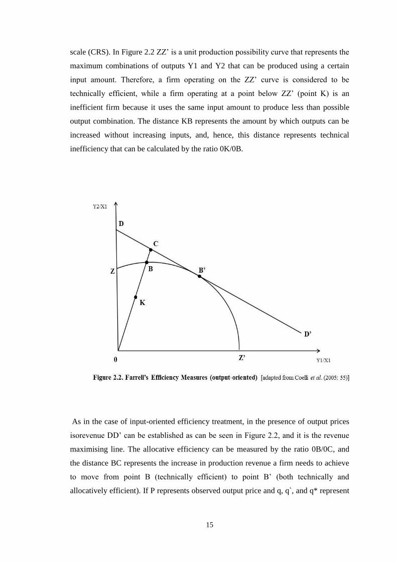
15

scale (CRS). In Figure 2.2 ZZ’ is a unit production possibility curve that represents the

maximum combinations of outputs Y1 and Y2 that can be produced using a certain

input amount. Therefore, a firm operating on the ZZ’ curve is considered to be

technically efficient, while a firm operating at a point below ZZ’ (point K) is an

inefficient firm because it uses the same input amount to produce less than possible

output combination. The distance KB represents the amount by which outputs can be

increased without increasing inputs, and, hence, this distance represents technical

inefficiency that can be calculated by the ratio 0K/0B.

As in the case of input-oriented efficiency treatment, in the presence of output prices

isorevenue DD’ can be established as can be seen in Figure 2.2, and it is the revenue

maximising line. The allocative efficiency can be measured by the ratio 0B/0C, and

the distance BC represents the increase in production revenue a firm needs to achieve

to move from point B (technically efficient) to point B’ (both technically and

allocatively efficient). If P represents observed output price and q, q`, and q* represent

16

output vector of firm associated with point K, point B, and point B’, respectively, then

Farrell’s efficiency measures are as follows:

;

(3)

And the output prices, also, can be utilised to calculate the revenue efficiency:

Given the measures of technical efficiency and allocative efficiency, the total overall

revenue efficiency can be expressed as a product of both measures as follows:

(4)

And as in the case of input-oriented measures, all the three efficiency measures are

bounded between zero and one.

If information on both input prices and output prices is available, then profit efficiency

can be calculated by combining the two analyses above into one analysis, taking into

consideration both cost and revenue efficiencies. In this sense, a profit efficient firm

maintains a production process at which the lowest costs are used to produce the

maximum revenues given input and output prices. In the methodology chapter, we will

present a comprehensive discussion on how to measure both cost and profit

efficiencies using the method of Stochastic Frontier Analysis (SFA).

2.3.2 Pure Technical and Scale Efficiency

Although a firm can be both technically and allocatively efficient, it might still operate

at a scale of operation that is not optimal. In the previous section we presented

efficiency measures based on constant returns to scale assumption, but this

assumption does not always hold. A firm might be operating within the increasing

returns to scale or within the decreasing returns to scale part of the production

function. In other words, the firm might be operating under the assumption of variable

returns to scale (VRS). Therefore, the technical efficiency, in general, can be

decomposed into pure technical efficiency (PTE) and scale efficiency (SE) (Coelli et

al., 2005). To illustrate how to calculate these two efficiency measures, we assume a

17

one-input, one-output production function considering the input orientation

perspective4 in Figure 2.3.

Firms operating at points F, B, and C are all technically efficient as they are operating

on the production frontier. However, firm F is operating within the increasing returns

to scale portion of the production frontier and can be more productive by increasing its

operating scale towards point B. Firm C, on the other hand, is operating within the

decreasing returns to scale of the production frontier and can be more productive by

decreasing its operating scale towards point B. A firm operating at point B, that is

located on the constant returns to scale frontier, is operating at the most productive

scale size or at the technically optimal productive scale (TOPS) and cannot be more

productive. Coelli et al. (2005: 59) state that, “A scale efficiency measure can be used

to indicate the amount by which productivity can be increased by moving to the point

of TOPS.” The firm represented by point D in Figure 2.3 is technically inefficient

4 A similar analogy can be followed to illustrate pure technical and scale efficiency measures under

output orientation perspective.

18

because it is operating below the production frontier. The pure technical efficiency

(PTE) of this firm under the VRS technology is equal to the ratio GF/GD, while the

scale efficiency (SE) is represented by the distance from point F to the CRS

technology and is equal to GA/GF. The value of SE is unity when operating at the

constant return to scale, as in the case of point B, while it is less than unity for firms F

and C because they are operating on the VRS frontier but not on the CRS frontier.

Thus, scale efficiency can be calculated by dividing total technical efficiency by pure

technical efficiency. Or alternatively, scale efficiency (SE) is equal to the ratio of

technical efficiency under the CRS assumption to the technical efficiency under the

VRS assumption;

= (GA/GD)/ (GF/GD) = GA/GF (5).

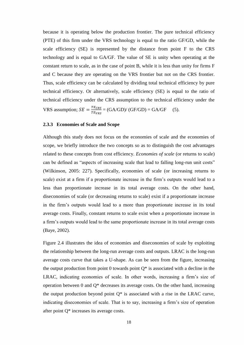
2.3.3 Economies of Scale and Scope

Although this study does not focus on the economies of scale and the economies of

scope, we briefly introduce the two concepts so as to distinguish the cost advantages

related to these concepts from cost efficiency. Economies of scale (or returns to scale)

can be defined as “aspects of increasing scale that lead to falling long-run unit costs”

(Wilkinson, 2005: 227). Specifically, economies of scale (or increasing returns to

scale) exist at a firm if a proportionate increase in the firm’s outputs would lead to a

less than proportionate increase in its total average costs. On the other hand,

diseconomies of scale (or decreasing returns to scale) exist if a proportionate increase

in the firm’s outputs would lead to a more than proportionate increase in its total

average costs. Finally, constant returns to scale exist when a proportionate increase in

a firm’s outputs would lead to the same proportionate increase in its total average costs

(Baye, 2002).

Figure 2.4 illustrates the idea of economies and diseconomies of scale by exploiting

the relationship between the long-run average costs and outputs. LRAC is the long-run

average costs curve that takes a U-shape. As can be seen from the figure, increasing

the output production from point 0 towards point Q* is associated with a decline in the

LRAC, indicating economies of scale. In other words, increasing a firm’s size of

operation between 0 and Q* decreases its average costs. On the other hand, increasing

the output production beyond point Q* is associated with a rise in the LRAC curve,

indicating diseconomies of scale. That is to say, increasing a firm’s size of operation

after point Q* increases its average costs.

19

Economies of scope exist when the total costs of producing two or more products

jointly is less than the total costs of producing those products separately or

independently (Molyneux et al., 1996). Conversely, diseconomies of scope occur

when the joint production of two or more products is more costly than separate or

independent production of those products. To illustrate this, consider a firm that

produces two outputs Q1 and Q2. If the two outputs are produced independently, their

separate cost functions are C (Q1, 0) and C (0, Q2), while, if they are produced jointly,

then their joint production cost is C (Q1, Q2). If the total costs of producing the two

outputs jointly is less than the combined cost of producing the two outputs separately,

then economies of scope exist and that can be expressed as C(Q1, Q2) < C (Q1, 0) + C

(0, Q2). If the inequality sign is reversed, then diseconomies of scope exist. For banks,

economies of scope can be exploited if producing multiple financial and banking

services jointly is less costly than producing those services separately, which would

lead to cost savings, and the reverse is true (diseconomies of scope exist) when the

joint production of services is more costly than the separate production of those

20

services. Given the example above, the overall economies of scope can be measured as

follows:

( ) ( ) ( )

( ) (6)

Where SCOPE > 0 indicates overall economies of scope and SCOPE < 0 indicates

diseconomies of scope.

2.4 The Measurement of Efficiency

In this section we present a brief overview of the frontier efficiency methods which

differ mainly in the assumptions of data regarding the functional form of the best-

practice frontier, whether or not random error is taken into consideration, and the

technique used to disentangle inefficiency term from random error if random error is

considered (Berger and Humphrey, 1997). We start by introducing the non-parametric

efficiency methods, then we present the parametric methods.

2.4.1 Data Envelopment Analysis (DEA)

Data envelopment analysis is a linear mathematical programming technique that can

be used to construct the efficiency frontier (best-practice frontier) against which the

relative performance of different homogenous entities called Decision Making Units

(DMUs) can be measured5. This method was suggested by Boles (1966), Shephard

(1970) and Afriat (1972); however, it was first applied by Charnes, Cooper and

Rhodes (CCR) (1978). Charnes, Cooper and Rhodes (1978) proposed the data

envelopment analysis as a mathematical programming technique based on input-

oriented model assuming constant returns to scale (CRS). This technique allows for

multiple inputs and outputs for a sample of decision making units (DMUs). Following

studies of data envelopment analysis, such as Färe, Grosskopf and Logan (1983),

Banker, Charnes and Cooper (BCC) (1984), extending the DEA method was suggested by

Charnes, Cooper and Rhodes (CCR) (1978) so as to be applied assuming variable

returns to scale (VRS). This method is called data envelopment analysis because the

5 For more comprehensive explanation, see [Färe et al. (1985), Ali & Seiford (1993), and Lovell

(1994)].

21

data for the best practice DMUs envelop the data for the rest of the DMUs in the

sample. The DEA frontier is formed as a linear combination of the best practice

observations that lead to the formation of a convex production possibility set. The

DEA is a technique that assumes that there are no random errors, so that all deviations

from the efficiency frontier are considered as inefficiency, and this is the main

difference between this approach and the parametric approaches, such as the stochastic

frontier analysis (SFA), as will be discussed later on in this section.

2.4.2 Free Disposal Hull (FDH)

The other non-parametric approach is the Free Disposal Hull (FDH) approach, which

is a special case of the data envelopment analysis (DEA). The FDH requires minimal

production technology assumptions compared to the other frontier approaches,

including the DEA. For instance, the FDH relaxes the assumption of convexity of the

production possibility set. The FDH approach was suggested as a new frontier method

for measuring productive efficiency by Deprins et al. (1984) and Tulkens (1986,

1993). De Borger et al. (1994) argue that the FDH approach has some advantages; for

example, it does not make strong assumptions concerning the production technology

and it is a non-parametric approach that does not depend on a particular parametric

form to be chosen in order to do the economic analysis. However, the authors state that

its major shortcoming is that it is “sensitive both to the number and the distribution of

the observations in the data set, and to the number of input and output dimensions

considered” (p.656). Moreover, Tulkens (1993) argues that the FDH is compatible or

interior to the DEA frontier and therefore it overestimates the average efficiency

compared to the DEA approach. Between the two non-parametric frontier methods

aforementioned, the DEA is much more popular and widely used in banking efficiency

studies compared to the FDH approach.

2.4.3 Stochastic Frontier Analysis (SFA)

As opposed to the non-parametric frontier approaches, the parametric frontier

approaches are more sophisticated and require functional forms and assumptions to

construct a stochastic optimal frontier to measure efficiency. In addition, parametric

approaches are capable of combining both technical and allocative efficiencies. The

best-known parametric technique and the most widely used for measuring efficiency

among others is the Stochastic Frontier Analysis (SFA) (it is also known as the

22

Economic Frontier Approach, EFA). The SFA was independently developed by

Aigner et al. (1977) and Meeusen and van den Broeck (1977) and was motivated by

the idea that not all deviations from the efficiency frontier might be under the control

of the management of the DMUs under study. The SFA specifies a functional form for

cost (or profit) frontier where a composed error term is considered so as to separate

inefficiency term from random noise using some distributional assumptions. The

random noise is assumed to follow a symmetric (two-sided) distribution while the

other non-negative part of the composed error term that represents inefficiency follows

a particular one-sided distribution.

To illustrate the idea upon which the SFA is built, we refer to a simple example of cost

efficiency function. Consider a single-equation stochastic cost function form:

( ) ( ) (7)

Where is the total costs, is a vector of outputs, is an input price vector, is a

two-sided noise component, and is a non-negative disturbance term that represents

inefficiency (the deviation from cost efficiency frontier). While the noise term is

usually assumed to follow a normal distribution, different distributional assumptions

with regard to the inefficiency term have been proposed. Those distributions range

from half-normal and exponential distributions proposed by Aigner et al. (1977) and

Mester (1993) to truncated normal and gamma distributions [Berger and Humphrey

(1997) and Kumbhakar and Lovell (2000)]. To obtain the parameters of the frontier

function and the composed error, maximum likelihood (ML) estimation or the

corrected ordinary least squares can be used. However, Kumbhakar and Lovell (2000)

argue that the ML estimation generates more efficient estimates by utilising the

distributional assumptions when the independence of factors and regressors matters.

We will discuss the stochastic frontier analysis (SFA) for panel data models in detail

in the methodology chapter.

2.4.4 Distribution Free Approach (DFA)

The distribution free approach (DFA) was developed by Berger (1993) following

earlier panel data approaches introduced by Schmidt and Sickles (1984). Similar to the

SFA, DFA specifies functional forms for the efficiency frontier, however, it differs

from the SFA in the way it disentangles inefficiency term from the random error. It

23

assumes that inefficiency is persistent over time and the random error tends to zero-

value over time as the random errors cancel each other by averaging. In the panel data

model, cost or profit functions are estimated for every period of the panel data where

the composed residual is comprised of inefficiency and random error terms. As the

random errors cancel each other over time, the average of residual from all the

regressions is an estimate of inefficiency.

The DFA has the advantage of easy implementation as it does not require strong

assumptions as to the distribution of inefficiency term or random error. For this reason,

and contrary to the SFA, the cost or profit function based on the DFA can be estimated

using generalised least squares (GLS), as done by Schmidt and Sickles (1984), or the

ordinary least squares (OLS), as done by Berger (1993). However, the main drawback

of the DFA is that it assumes that efficiency is persistent over time and the random

error tends to zero-value average over time. Therefore, if the study period is too long

then inefficiency might not be persistent over time, or if the study period is so short

then error terms might not cancel each other, which might all generate misleading

results.

2.4.5 Thick Frontier Approach (TFA)

The thick frontier approach (TFA) was developed by Berger and Humphrey (1991), and

it differs from the other frontier parametric approaches in terms of the estimation of

efficiency frontier. This approach estimates cost/profit function for the lowest/highest

average cost/profit quartile of firms (considered as thick frontier), where firms’

efficiencies are higher than the sample average efficiency, rather than estimating a

precise efficiency bound. Moreover, a cost/profit function for the highest/lowest

average cost/profit quartile is estimated too, where firms’ efficiencies are lower than

the sample average efficiency. The main assumption here is that the difference

between the two cost/profit functions (related to the highest and the lowest quartiles) is

attributed to inefficiencies and exogenous factors, while the error terms within the

highest and lowest quartiles represent measurement error and luck. This approach is

not widely used in banking efficiency studies because the aforementioned assumption

is difficult to be held exactly, resulting in imprecise estimates of banking

inefficiencies, in addition to the problems of skewing and heteroskedasticity of error

terms that might result from dividing data into quartiles (Matousek and Taci, 2004).

24

Furthermore, a main disadvantage of this approach is that it does not provide estimated

efficiency scores for individual firms, rather it provides an estimate of average

efficiency for the whole tested sample. However, Berger and Humphrey (1991) argue

that their main purpose of using the TFA is to obtain a basic idea as to the likely

magnitude of efficiency and not to get an exact efficiency measurement.

2.4.6 What is the Best Frontier Method?

There is no consensus as to what frontier method is preferred for measuring banking

efficiency, but the stochastic frontier analysis (SFA) and data envelopment analysis

(DEA) are the most widely used efficiency frontier methods among the others

discussed above (Berger and Humphrey, 1997). As the data envelopment analysis

(DEA) is a non-parametric approach and the stochastic frontier analysis (SFA) is a

parametric approach, then there must be differences in the application and the

assumptions of both approaches. It is important to highlight such differences as only

one approach (the stochastic frontier approach) will be adopted in this thesis. The

advantage of the DEA method is that it is simple to apply because no functional forms

and preliminary restrictive assumptions are needed, and it performs well with small

sample of firms. In addition, as Oral and Yolalan (1990) argue, DEA performs well

and provides meaningful efficiency results when firms use similar resources to provide

similar services. The major disadvantage of the DEA is that it does not account for

random errors6 and therefore it considers all deviations from the efficiency frontier as

inefficiencies resulting in the inclusion of exogenous variables in the inefficiency

term, hence the inefficiency term might be overestimated [Berger and Humphrey

(1997); Coelli et al. (2005); Weill (2003) and Murillo-Zamorano (2004)]. Another

shortcoming of the DEA is that it is very sensitive to outliers because it envelops the

outlier observations even though those outliers might be the result of an error and not

real ones (Sarafidis, 2002, Havrylchyk, 2006).

On the other hand, the SFA is a stochastic approach that uses econometric tools to

estimate efficiency frontier. The main weakness is that it “impose[s] more structure on

the shape of the frontier by specifying a functional form for the cost [or profit]

function” (Weill, 2003: 579). However, the main advantage of the SFA is that,

contrary to the DEA, it allows for random error by using a composed error model

6 For more on this shortcoming, see [Berger and Humphrey (1997) and Coelli et al. (2005)].

25

where inefficiency follows an asymmetric distribution (e.g. half normal, gamma,

truncated normal) and random error follows a symmetric distribution (usually the

standard normal). Therefore, the SFA provides the technique by which the inefficiency

term can be disentangled from the error term, resulting in an unbiased estimation of

inefficiency differences that are under the control of the firm’s management and

independent of exogenous factors [Berger and Humphrey (1997) and Hollo and Nagy

(2006)]. In this thesis the stochastic frontier analysis (SFA) is the approach chosen to

measure bank efficiency for the advantage mentioned above, where the random error

is taken into account and inefficiency term can be disentangled from error term using

some distribution assumptions. The sample used in this thesis is large, combining

banking sectors in the European Union 27 member states, where there might be

heterogeneity and different exogenous factors affecting banking efficiency scores and

need not be included in the inefficiency term. Also, the SFA can account for risk

preference and environmental differences between countries and banks which allow

for more robust and unbiased efficiency estimates, while DEA does not allow for that

(Weill, 2003). Moreover, as mentioned earlier, DEA approach performs better with a

small sample which is not the case in this study, hence the SFA is superior and more

suitable to be used in this study.

2.5 Risk in Banking Institutions

As this study will investigate different types of risk and the link between such risks

and bank efficiency and stock performance, we briefly shed light on risks in banking

institutions in this section. Commercial banks engage in different related activities that

range from providing products and services to customers to intermediation and risk

management. Risk management has to be an important issue to be considered when

studying the activities of commercial banks. Merton (1989: 243) states that “an

important part of the management of financial intermediaries is the management and

control of the risk exposures created by issuing their financial products.” Saunders and

Cornett (2006) add that modern financial institutions are in the risk management

business as they bear and manage risk on their customers’ behalf by pooling risks and

selling their services as risk specialists. This section aims at introducing an overview

of banking risks and analysing the relationship between risk and return. The Capital

26

Asset Pricing Model (CAPM) is utilised to explain the trade-off between risk and

return on an investment. Four banking risks are explained in this section; namely,

insolvency risk, credit risk, liquidity risk, and market risk. Although banks face other

types of risks, these risks are chosen because they will be adopted in this thesis to

examine their level and their effects on bank efficiency and stock returns. Finally, the

important role of bank capital in reducing risks and enhancing banking sector stability

is highlighted through a brief discussion of the capital requirements based on Basle

Accords.

2.5.1 Banking Risks Overview and CAPM

Risk in finance can be defined as the probability of making profits or losing money on

an investment, or as Howells and Bain (2008) argue that risk is the probability that the

actual return might not be the same as the expected return. Also, risk can be looked at

as the uncertainty surrounding the outcome that would take place in the future, where

more than one possible outcome might occur. The investigation of bank risk has led to

different risk classifications proposed by authors based on their analytical purposes.

For instance, Vyas and Singh (2011) argue that risk faced by banks belong mainly to

two general groups. The first group is transactional risks, under which category market

risk and credit risk are listed. The second group is operational risks that Vyas and

Singh (2011: 17) define as “a risk arising from execution of a company’s business

functions [such as] fraud risks, legal risks, physical or environmental risks, etc.”

Greuning and Bratanovic (2009) classify bank risk into three categories; financial,

operational, and environmental risks. Rose (1999) divides bank risks into six types;

credit risk, liquidity risk, market risk, interest rate risk, earning risk, and solvency risk,

while Jorion (1997) refers to three types of bank risks; business risk, strategic risks,

and financial risks.

In general, there is a trade-off between risk and return on an investment. In other

words, one would not invest in a risky investment unless they receive a return to

compensate them for the risk implied by that investment, because people, in general,

are risk-averse. To illustrate the relationship between risk and return, Sharpe (1964)

and Lintner (1965) developed a capital asset pricing model (CAPM) that attempts to

explain the relationship between risk and return on a financial security that helps

determine the fair price of such security. The CAPM is based on the idea that if a

27

security helps to stabilise a portfolio by making it in line with the market, then this

security should earn a similar return as the market portfolio. While if the security

increases the risk of a portfolio compared to the market portfolio, then the demand on

this security will decrease by risk-averse investors leading its price to fall and its

expected return will be higher than the market return. On the other hand, if the security

makes a portfolio less risky compared to the market portfolio, then it will be in higher

demand, leading its price to rise and its expected return to fall below the market return.

Based on some assumptions, such as the existence of perfect or efficient market,

investors are risk-averse, and no transaction costs exist, CAPM is defined by the

following equation where only systematic risk is priced and measured by beta (β):

( ) ( ) (8)

Where ( ) is the expected return for a security (or asset) i, is the risk-free rate of

return available for investors, is the measure of systematic risk (beta) for security i,

and ( ) is the expected return on market portfolio7.

2.5.2 Insolvency Risk

Insolvency risk for a bank can be defined as “the potential disability of a bank to raise

enough cash timely in order to meet payment obligations [and hence becomes

insolvent]” (Matz and Neu, 2007: 178). This risk is closely related to financial gearing

(leverage) as banks are highly leveraged (maintain high ratio of debt/equity) compared

to other institutions. A bank must have enough capital (equity) in order to be able to

absorb potential losses that might result from taking on excessive risks and hence

remain solvent (has a positive net worth of shareholders’ equity), otherwise it might be

forced into liquidation. Therefore, as bank capital is the difference between its assets

and liabilities value, insolvency or capital risk refers to the decrease in the market

value of its assets below the market value of its liabilities (Casu et al., 2006). In this

sense, bank capital is the cushion against the risk of failure by absorbing financial and

operating losses until management becomes able to solve the bank’s problems and

restore its profitability (Rose, 1999). For this reason, a bank with higher risk taken

should maintain greater amount of capital, and this is the principle behind the Basle

capital requirements (as will be explained later in this chapter).

7 7 For more on CAPM, see [Arnold (2008) and Pilbeam (2005)].

28

Banks usually prefer to hold less capital and larger debts to finance their investments

because of the higher costs associated with raising equity capital. In general, as Arnold

(2008) argues, raising capital by issuing new shares is more costly than obtaining

loans (debts) because of the direct costs associated with issuing shares and more

importantly, because the rate of return required by shareholders is higher than the rate

of return (interest rate) on issuing bonds (debts). Also, shareholders’ dividends are

paid out of after-tax profits, while interest payments on loans are tax deductible.

Moreover, higher capital means lower returns on equity holders because, as discussed

by Mishkin and Eakins (2012), the return on equity (ROE) is negatively related to

equity capital according to the following equation:

( ) ( )

( ) (9)

Therefore, banks prefer to maintain less capital so as to reduce their costs and increase

their profits, or in other words, banks tend to maintain less capital in order to increase

their cost and profit efficiencies.

2.5.3 Credit Risk

Credit risk can be defined according to the Basle Committee on Banking Supervision

(2000: 1) as “the potential that a bank borrower or counterparty will fail to meet its

obligations in accordance with agreed terms.” Tapiero (2004) argues that with regard

to credit risk, uncertainty stems from two sources: default by a party to a financial

contract or changes in the present value of future cash flows that might result from

fluctuations in the financial market conditions or changes in the economic

environment or interest rates. Banks’ management should give close attention to the

creditworthiness of their borrowers so as to decrease the probability of default on their

loans, and hence decrease the probability of bank failure as banks usually tend to hold

little equity capital. Bank managers must decrease the amount of credit losses by

building a diversified portfolio and should investigate the ability of their borrowers to

pay their loans before and after they issue the loans.

As loans usually constitute the largest part of banks’ assets, it is highly important for

banks to decrease the credit risk associated with issuing loans by setting up sound

standards to investigate the creditworthiness of banks’ borrowers. One measure of

bank credit risk is the ratio of non-performing loans to total gross loans, the higher this

29

ratio is, the higher the level of credit risk that a bank has. With higher level of credit

risk, costs related to monitoring, screening, working out loans, or selling bad loans

increase, this in turn decreases the cost efficiency of the bank. Furthermore, the higher

the level of credit risk associated with higher non-performing loans (for example), the

higher the costs associated with monitoring and working out, selling, or writing-off the

bad loans and the higher the expenses related to the loan-loss provisions. This in turn

would decrease banks’ profits and therefore would lead to lower bank profit

efficiency.

2.5.4 Liquidity Risk

Liquidity (or funding) risk can be defined as the potential that a bank (or a firm) will

be unable to meet its obligations as they fall due because they lack the ability to

liquidate some of their assets or raise enough funding from new source at reasonable

costs. Banks must have sufficient cash and borrowing capacity in order to meet

deposits withdrawal, net loan demand, and other cash needs (Rose, 1999). As it might

be confusing, Hull (2010) distinguishes solvency from liquidity. He argues that

solvency refers to the idea that a bank has more assets than liabilities and hence its

equity capital is positive. On the other hand, liquidity refers to the ability of a bank to

make cash payments as the fall due. Liquidity risk might result from a mismatch

between the size and the maturity of assets and liabilities in a bank’s balance sheet.

For instance, if a bank is not able to meet deposit withdrawals, this might lead to a

bank run where depositors rush to withdraw their deposits as a consequence of losing

confidence in the bank. This, in turn, might limit the ability of the bank to borrow

funds from the interbank market, turning the liquidity crisis of the bank into solvency

crisis and possible failure.

To reduce liquidity risk, banks can increase the proportion of liquid assets of cash and

marketable securities, such as Treasury bills (T-bills) and other government securities,

or fund its operation using longer-term liabilities. However, holding such liquid assets

might decrease the profitability of the bank as the rate of return associated with such

assets is lower (Casu et al., 2006). Banks with higher liquidity risk (less liquid assets)

might be forced to borrow emergency funds at higher rate of return, which in turn

increase bank costs and decrease bank cost efficiency. However, because liquid assets

yield lower rate of return for the bank compared to other risky assets, such as loans,

30

higher amount of these assets might decrease bank profits and hence its profit

efficiency.

2.5.5 Market (or Trading) Risk

Casu et al. (2006: 269) define market risk as “the risk of losses in on-and-off- balance

sheet positions arising from movements in market prices [and it is particularly related]

to short-term trading in assets, liabilities and derivative products, and relates to

changes in interest rates, exchange rates and other asset prices.” For instance, a bank

might suffer losses resulted from changes in the prices of fixed-income instruments,

equity instruments, commodities, currency contracts, or changes in the market indices

overall. Greuning and Bratanovic (2009) argue that the major components of market

risk are interest rate risk, equity risk, commodities risk and currency risk. Banks must

keep up with any changes in the overall market conditions because such changes will

affect the overall performance of banks. Rose (1999) discusses as an example that as

interest rates increase, the market value of fixed-income securities (e.g. bonds) and

fixed-rate loans will fall. Conversely, as interest rates decrease, the market value of the

banks’ fixed-income securities and fixed-rate loans will increase, generating capital

gains when they are sold, but the bank might suffer losses on its fixed-rate liabilities.

Casu et al. (2006) refer to the risk associated with unexpected changes in interest rates

as interest rate risk whose effects depends on whether bank assets and liabilities are

fixed rate or rate-sensitive8. Value-at-Risk (VAR) analysis is one method that larger

banks perform to assess the market risk associated with their trading assets portfolios

whereas small banks conduct sensitivity analysis to measure market risk (Casu et al.,

2006).

2.5.6 Capital Requirements and Bank Risks

Capital acts as a cushion against losses that might result from taking on excessive risks

by the bank’s management. To maintain the soundness and safety of banks and keep

the financial system stable, financial regulators have paid close attention to the capital

adequacy. While banks prefer to operate with less capital so as to maximise the return

on equity as banks’ returns depend on risk taken, regulators require banks to increase

their capital to keep safer. To reduce bank risks including insolvency risk, credit risk,

8 For more on interest rate risk, see Casu et al. (2006).

31

liquidity risk and market risk, the Basle Committee has proposed different agreements

(known as Basle Accords) that specify minimum capital requirements to be applied by

banks. The first was the Basle I Accord that was proposed in 1988 and came into

effect in 1992. This accord set a minimum capital equal to 8% of the risk-weighted

assets (defined by Tier 1 and Tier 2) to be held by financial institutions so as to

address credit risk and the risk of a counterparty defaulting on its obligations. In spite

of its simplicity, Basle I Accord was criticised because it only considers credit risk and

it uses uniform risk-weight categories, making the capital requirements specified by

this accord insufficient to protect banks against risk and maintain the stability of the

financial system.

As a consequence of the flaws associated with Basle I Accord, Basle Committee

proposed new rules to update Basle I Accord in 1999, the modified version of Basle

Accord I after taking significant amendments into consideration was adopted and

published in 2004 under the name of Basle II Accord. The aim of Basel II Accord was

to adopt more comprehensive sensitive risk-measure that allowed banks to use their

own estimates of risk to determine minimum capital requirements. According to Basle

II9, market risk (after amendments in 1996) and operational risk along with credit risk

were taken into account and the minimum capital requirement remained unchanged at

8%. Furthermore, two new pillars were added to the first pillar, which is related to the

minimum capital requirements (Tier 3 introduced). The first new pillar relates to the

supervisory review process where regulators in different countries can take their local

conditions into account when applying Basle II rules. The second new pillar is

concerned with market discipline where banks are required to disclose more

information about their capital and risk [(Hull, 2010) and (Greuning and Bratanovic,

2009)].

The global financial crisis 2007-2009 and the huge losses for banks associated with

this crisis raised concerns about the ability of Basle II Accord to prevent losses and

strengthen the immunity of banks against financial fluctuations and economic

environmental turmoil. As a consequence of the weaknesses revealed in Basle II, the

Basle Committee developed Basle III in 2010-2011, aimed at strengthening the

9 For more detailed discussion on Basel II, see [Hull (2010) and Greuning and Bratanovic (2009)].

32

resilience of the banking sector. Basel III strengthens the capital adequacy

requirements in terms of quality and quantity and introduces new requirements with

regard to bank liquidity and bank leverage (King and Tarbert, 2011). The adoption of

Basel III Accord followed a thorough discussion by the G20 leaders in 2008 and 2009

regarding what should be done so as to strengthen and enhance the global financial

regulation and supervision as the global crisis hit strongly. The leaders reached an

agreement with regard to enhancing capital requirements, discouraging high levels of

leverage, introducing better liquidity risk requirements, and developing sustainable

frameworks to deal with securitisation, compensation practices, and moral hazards

risks (ECB, 2010) [for more on Basle III and its previous versions see Eubanks

(2010a), Monroe (2010) and King and Tarbert (2011)].

2.6 World Financial Crisis

In this study the effect of the world financial crisis on bank efficiency and bank stock

performance is investigated. Therefore, in this section we briefly discuss the evolution

of the world financial crisis, how it started in 2007 in the US market, and the causes

that might be behind the occurrence of such a financially severe event. Also, we shed

light on the relationship between different kinds of financial risks, such as; insolvency

risk, credit risk, and liquidity risk and the world crisis.

2.6.1 Overview of the World Financial Crisis

The world financial crisis has been said to be the most severe global economic disaster

in the last 80 years, and some economists, financial analysts, and researchers consider

it even worse than the Great Depression in the 1930s. The main source and the trigger

for this world crisis that resulted in a severe global recession was the subprime10

mortgage market that collapsed after the housing bubble burst in the United States in

2007. This caused a financial and economic turmoil that spread globally out of the US

economy due to financial integration and economic globalisation around the world.

Calverley (2009: 107) states that, “The crisis was a direct result of too much mortgage

lending, which went bad when the housing bubble burst.” This financial crisis has not

10

Subprime loan refers to a loan that is due to its higher probability of default and is considered to be

riskier than the normal (prime) loan (Demyankyk and Hasan, 2010).

33

only driven world stock markets to fall, but it has also caused many financial

institutions including large banks to be taken over, merged, nationalised, bailed out,

declared insolvent or liquidated. Among those financial institutions is Lehman

Brothers, which was the largest investment bank in the US, and was filed into

bankruptcy in September 2008 as a result of investing heavily in mortgage-backed

securities (MBS) and other collateralised debt obligations (CDOs). Bear Stearns, a

global investment bank in the US, suffered big subprime mortgage losses in two of its

hedge funds in June of 2007 and was sold later to JPMorgan Chase in 2008. Also,

Citigroup was one of the biggest financial services companies in the world before it

was bailed out by the US government in 2008 due to huge losses it suffered during the

crisis time. Fannie Mae and Freddie Mac, the two largest mortgage finance lenders,

were taken into conservatorship by the US Treasury after they failed to maintain

adequate capital ratio over the crisis period (Calverley, 2009). In the UK, Northern

Rock, a retail and mortgage bank, was nationalised by the U.K. government in 2008

after suffering big losses caused mainly by default of mortgage borrowers on their

loans (Eiteman et al., 2009).

There has been a range of causes behind the world financial crisis that have been

discussed by authors and economists. One main cause that has been criticised for

contributing to the global financial crisis by creating very complicated financial

instruments is securitisation11

, as argued by Mishkin and Eakins (2012), Shin (2009),

Martin-Oliver and Saurina (2007), Keys et al. (2008), Calomiris (2009), Thomas

(2010), and Diamond and Rajan (2009). The high level of leverage (borrowing)

maintained by financial institutions prior to the crisis, also, has been argued by the US

government Accountability Office (2010), Blundell-Wignall and Atkinson (2009), and

Carmassi et al. (2009) to be a major contributor to the crisis by increasing the risk of

bank failure. The risk of liquidity faced by financial institutions prior and over the

beginning of the crisis time is further discussed to be a major cause of the financial

crisis as explained by Brunnermeier (2009) and Diamond and Rajan (2009). The loose

monetary policy (especially interest rate) that was adopted prior to the financial crisis

by monetary authorities in the US and other countries is, according to Taylor (2008),

11

Kendall and Fishman (2000: 1) define securitisation as “a process of packing individual loans and

other debt instruments, converting the package into a security or securities, and enhancing their credit

status or rating to further their sale to third-party investors.”

34

Calomiris (2009), and Brunnermeier (2009), an important participant in causing the

crisis. Moreover, the too-big-to-fail doctrine that urged many large financial

institutions to take on excessive risk (moral hazard) as taxpayers will share that risk

with them in bad times is blamed for contributing to the crisis by Zingales (2010) and

Calomiris (2009). In addition to the aforementioned factors, other causes of the crisis

are the excessive compensation schemes, as argued by Blinder (2009), Diamond and

Rajan (2009), Caprio et al. (2010), and Lang and Jagtiani (2010), the credit rating

agencies, as discussed by Lang and Jagtiani (2010), Calomiris (2009), and Hunter

(2008), and imprudent government regulations and policies, as clarified by Calomiris

(2009). Other studies that investigate the causes of the world financial crisis are

Merrouche and Nier (2010), Eisenbeis (2010), Claessens and Kose (2010), Mishkin

and Eakins (2012), and Poole (2010).

Demirguc-Kunt and Serven (2010) argue that actions taken in the US and European

countries include inserting huge amount of liquidity, providing assurance to creditors

and depositors supported by blanket guarantees, bailout schemes, recapitalisation, and

obtaining a large share in financial institutions by governments, in addition to setting

provisions of credit to non-financial firms. However, different recommended solutions

have been proposed to overcome the problems contributed to the occurrence of the

world financial crisis. For instance, Calomiris (2009) suggests regulatory reform

procedures that might enhance risk management and banking system to avoid such

severe crisis in the furfure. Those procedures are related to developing prudential

micro capital regulations by finding efficient instruments to accurately measure assets

risk, and also related to adopting capital requirements that are flexible to meet

macroeconomic circumstances. Moreover, the author suggests that large complex

financial institutions should be required to prepare credible pre-packaged and pre-

approved resolution plans to control the problem of too-big-to-fail. Also, the author

suggests modification to the terms of issuing housing loans to reduce mortgage default

risk and retracing ownership at banks to solve the agency problems that might exists.

Lang and Jagtiani (2010), Caprio et al. (2010), and Blinder (2009) have proposed

solutions to alleviate the negative consequences associated with massive compensation

schemes on risk management. While Blundell-Wignall and Atkinson (2009) propose

suggestions to reform financial regulations, Carmassi et al. (2009) and Zingales (2010)

suggest solutions to reduce systematic instability and controlling the bad consequences

35

of the too-big-to-fail doctrine by utilising new reliable capital requirements. Other

studies that suggest some solutions to the causes of the crisis are Caprio et al. (2010),

Diamond and Rajan (2009), Haldane (2009), and Demirguc-Kunt and Serven (2010).

2.6.2 World Financial Crisis and Banking Risks

There is a strong correlation between the world financial crisis and the risk taken by

financial institutions by the time of the crisis. The high level of risk taken by banks

and other financial institutions led many of those institutions into failure in the US and

Europe, in particular. One risk that has been highlighted when investigating the causes

and the characteristics of the financial crisis is insolvency (capital) risk. As discussed

above in this section, banks with higher capital are less risky because capital works as

a cushion to absorb losses a bank might encounter on their assets. Therefore, less

capital (higher leverage) threatens the existence of a bank by exposing it to higher

financial risk. The building up of financial leverage, in spite of the financial

regulations, by financial institutions prior to the world financial crisis has contributed

to the occurrence of that crisis. A study done by the US Government Accountability

Office (2010) argues that leverage ratio of five large broker-dealing holding

companies in the US grew from 22 to 1 in 2002 to around 30 to 1 in 2007.

Blundell-Wignall and Atkinson (2009), in their study on the crisis origins and

requirements for reform, discuss how leverage increased over the period prior to the

financial crisis at US and European banks. They show that the leverage ratio rose to

about 40: 1 in European and US investment banks, and to almost 20: 1 in the US

commercial banks between 2002 and 2007. This increase in the leverage ratio was

accompanied by acceleration in securitisation in the off-balance sheet mortgages, and

both actions were results of inefficient financial regulations that allowed financial

institutions to arbitrage capital and other requirements. Carmassi et al. (2009)

emphasise that due to financial innovation (particularly securitisation) the leverage in

financial institutions was magnified. That happened by removing risky assets off the

balance sheets, by reducing capital requirements using risk alleviation techniques

including credit derivatives, and by embedding leverage in the toxic waste (equity

tranches) of mortgage-backed securities. In addition, the authors argue that between

1999 and 2007 the aggregate leverage (total credit to GDP) increased by almost 80%

in the US and 100% in Europe in the wider economy, and by roughly 40% in the US

36

and 70% in Europe in the financial sectors, and that these high leverage percentages

contributed to amplifying the financial crisis.

Another bank risk that has been highlighted as a cause and a main phase of the world

financial crisis is liquidity risk. Liquidity risk faced by financial institutions before the

financial crisis time is highlighted by many studies. One of those studies is one

conducted by Brunnermeier (2009) on the liquidity and credit crunch 2007-2008. The

author argues that the reduction in funding liquidity, which contributed to the financial

crisis by leading to significant stress for financial systems, was caused by the maturity

mismatch at financial institutions. The exposure to the maturity mismatch had two

forms; the first is liquidity backstops, guaranteed by commercial and investment banks

for the off-balance sheet vehicles that were sponsored by those banks. Those vehicles

invested in long-term assets and borrowed for short-term periods (e.g. short-term

asset-backed commercial papers). In case those vehicles could not raise money from

short-term commercial bank papers to meet short-term obligations, commercial and

investment banks sponsoring the vehicles would be responsible for bearing the

liquidity risk caused initially by investing in the long-term asset-backed securities. The

second form of maturity mismatch exposure is the increased reliance of investment

banks on the short-term repurchase agreements (repos) causing maturity mismatch on

their balance sheets. Brunnermeier (2009: 80) states that, “This greater reliance on

overnight financing required banks to roll over a large part of their funding on a daily

basis.” Diamond and Rajan (2009) also argue that the short-term debt that attracted

financial institutions before the financial crisis was a major cause of it. While

investing heavily in long-term securities (mortgage-backed securities) and while they

were expecting low interest rate in the future, those financial institutions were actually

exposed to liquidity risk as they borrowed with short-term debt. When house prices

started to decrease causing mortgage-backed securities values to fall down, those

financial institutions, investing heavily in MBSs, found it difficult to borrow even with

short-term debts, making them illiquid due to the maturity mismatch problem.

Another important bank risk revealed by the world financial crisis is credit risk that

large financial institutions’ management took on at high levels prior to the crisis.

Many factors contributed to the high level of credit risk at large banks and other

financial institutions by the time of the world financial crisis. Among those factors is

the process of securitisation. Martin-Oliver and Saurina (2007) discuss that while

37

securitisation allows banks to increase liquidity, transfer credit risk, or arbitrage capital

requirements, it also increases the banks’ revenues from fees obtained by originating

and packaging loans subject to the securitisation process. The authors argue that

securitisation (originate to distribute) model has the problem of causing the incentives

for lenders to appropriately monitor and investigate the creditworthiness of borrowers

to disappear as a bank is going to get rid of the credit risk shortly. Thus, banks lower

their lending standards when lending mortgages to subprime borrowers, resulting in

high credit risk levels. This result is supported by Keys et al. (2008) who investigate

the linkage between securitisation and screening standards in the subprime mortgage

market in the US and find that the impact of securitisation reduces the motivation of

lenders to appropriately monitor and screen their borrowers in the mortgage market.

Another factor that might have led to increasing bank credit risk is the too-big-to-fail

doctrine that urged many large banks to take on excessive risk. Zingales (2010) argues

that the moral hazard caused by such a policy does not only take a form of excessive

risk that managers of large banks take on, but also the incentive of such large banks to

leverage up as they are capable of borrowing at cheap price from creditors who believe

that their debtors are protected by government guarantee. The too-big-to-fail is

criticised by Calomiris (2009) who emphasises that in addition to the very risky

activities that managers of large banks would invest in, “banks that are protected by

the government from the discipline of the market place will be too tolerant of bad

management, since managerial errors normally punished by failure will be hidden

under the umbrella of government protection.” (p.72)

The excessive compensation schemes adopted by many financial institutions were a

crucial factor in increasing the credit risk and bank risk overall at those institutions. In

his paper, which investigates the role of compensation in the financial crisis, Blinder

(2009) blames what he calls “go-for-broke” incentives that urge bankers to either take

on high-risk activities and get exacerbated compensations in case those bets generate

high return or otherwise get no bonuses and find new jobs, in such cases, losses are

absorbed by people’s money. Diamond and Rajan (2009) investigate the negative role

of generous compensation schemes in the risk management performance. The authors

notice that many of the compensation schemes were paid for short-term risk-adjusted

performance that motivated traders at financial firms to take risky activities whose

returns appeared, mistakenly, to come from better performance rather than from higher

38

risk premium. However, Diamond and Rajan (2009) argue that risk managers were not

ignorant of such incentives provided to risk traders (and enhanced by talent

competition between them), but managers might be unable to quantify and control

such incentives.

In this thesis, we will be investigating the level of the above three types of risk;

insolvency risk, liquidity risk, and credit risk, at banking sectors in the European

Union over the period 2004-2010. This allows us to investigate the level of these bank

risks before and during the world financial crisis, and also to compare the level of

bank risks for the entire EU, the old EU members, the new EU members, and the

GIIPS countries. Moreover, the effect of these types of bank risk on bank cost and

profit efficiencies and on bank stock returns will be examined. If empirical evidence

that banks with lower levels of these bank risks appear to be more efficient during the

financial crisis (2007-2009) than their counterparts with higher risk levels, then these

banking risks are important factors to control for in order to protect banking

performance during times of financial distress. Furthermore, the influence of the world

financial crisis on bank cost and profit efficiencies and on bank stock returns will also

be considered thoroughly in this thesis.

2.7 Eurozone Debt Crisis

The world financial crisis 2007-2009 has paved the way for another crisis named as

the Eurozone Sovereign-Debt Crisis. After the financial crisis and particularly from

2010, the financial markets have been highly affected by concerns regarding the

solvency of some European countries. These concerns focus mainly on the sovereign

debts in the Eurozone because of the weak performance of the so-called GIIPS 12

countries; namely, Greece, Ireland, Italy, Portugal, and Spain. The Eurozone debt

crisis started in Autumn of 2009 when the Greek government revealed a high

government deficit level of 12.7%, which is four times higher than the European Rules

(3% in the Maastricht Treaty) allow, and high public debt percentage. As a

consequence, the investors’ confidence eroded, which in turn caused interest rates on

government bonds to rise to high levels making it difficult for the Greek government

12

Some authors, policymakers and analysts refer to these countries as “periphery” countries, but in this

thesis we use the term GIIPS.

39

to borrow at a cheap price. The fear spread quickly to other members of the Eurozone,

particularly the GIIPS countries, as they all had budget deficits of GDP higher than the

allowed limit and high borrowing percentage. Such financial fears in the Eurozone and

the consequences that might appear as a result made the European Union and the

International Monetary Fund (IMF) intervene and provide financial assistance

packages to those countries facing sovereign-debt problems. As a consequence of the

debt crisis, the five GIIPS countries have been threatened by severe recession and their

government bonds have had junk ratings, BBB+ or lower by Standard & Poor’s, which

makes it difficult for them to sell large amount of bonds to finance their deficit or to

roll over a large public debt [Nelson et al. (2012) and Arellano et al. (2012)].

According to Nelson et al. (2012), the Eurozone crisis was a consequence of a

combination of challenges some of which faced the Eurozone countries together and

others which were specific to each country. The authors argue that capital inflows and

the following accumulation of public and private debt over the past decade into the

GIIPS states contributed to the crisis. As those countries prepared to adopt the Euro,

interest rates on their bond fell so as to converge with that of stronger economies of

the Eurozone, such as Germany. Thus, public and private sectors of the GIIPS

countries were able then to borrow more cheaply as they accessed new cheap credit,

but they did not use such capital efficiently in productive investments that could

generate enough money to repay their debts, which in turn increased debt levels. Also,

capital inflow increased prices and the overall inflation in the GIIPS countries, leading

to a decrease in their competitiveness with other Eurozone countries. As a result, these

countries had a deficit in their trade balance, forcing them to borrow and increase their

debts. Nelson et al. (2012) discuss that Greece had a poor management of public

finance with high levels of tax evasion as well as high government spending on public

sector jobs and benefits. With regard to Ireland, the budget deficit rose to over 30% as

a consequence of government guarantee and bailout of Irish banks, while the

Portuguese economy faced a problem of strengthening its competitiveness and was

progressing very slowly compared to the other Eurozone countries prior to the world

crisis. Spain, on the other hand, had budget surplus and low public debt prior to the

world crisis, however, capital inflows contributed to an unsustainable housing bubble.

As to Italy, this country has a long-term high public debt and tried to pay high wages

while having an under-competitive economy, leading to a budget deficit crisis.

40

Neri and Ropele (2013) argue that there is no solid evidence that the sovereign debt

crisis has macroeconomic effects on euro area as a whole and on individual countries.

Moreover, the authors argue that this crisis has led to an increase in the cost of new

loans and a contraction in credit which in turn caused negative effect on industrial

production in the GIIPS and other Eurozone countries. Furthermore, Allen and

Moessner (2012) point out that the lending capacity of banking systems in the euro

area has been much weakened as a consequence of the sovereign debt crisis. In

addition, the authors argue that the euro crisis has created internationally liquidity

stresses.

In this thesis, we utilised the Eurozone crisis by focusing on the performance of the

five GIIPS countries over the study period. We make an EU sub-sample of the GIIPS

countries to see how their cost and profit efficiency levels can be compared to that of

other EU groups. In addition, the three types of banking risk discussed above in this

chapter will be investigated to see what level they have prior to and during the world

financial crisis in these countries.

2.8 Summary and Conclusion

This chapter presents a theoretical framework concerning productive efficiency.

Inefficiency of a firm is measured as the deviation from a “best-practice” frontier

where totally efficient firms operate. Economic efficiency can be divided into

technical and allocative efficiency. Technical efficiency refers to the ability of a firm

to obtain the maximum level of outputs given a set of inputs, or the ability of a firm to

minimise input use in the production given a set of outputs. Allocative efficiency

reflects the ability of a firm to use the optimal proportion of inputs given their

respective prices and production technology. Technical efficiency can be decomposed

into pure technical and scale efficiency. Moreover, this chapter defines cost and

revenue efficiencies when information on input prices and output prices, respectively,

are available. Economies of scale refers to increasing firm scale that leads to falling

long-run unit costs, while economies of scope exist when the total costs of producing

two or more products jointly is less than the total costs of producing those products

separately or independently.

41

This chapter also reviews five (non-parametric and parametric) frontier approaches

that can be used to measure firm efficiency. The non-parametric approaches are

mathematical programming approaches that do not allow for noise when measuring

efficiency and hence consider all deviations from the frontier as inefficiency. The

parametric approaches, on the other hand, allow for noise when measuring efficiency

but they need a pre-specified functional form for the efficient frontier and the

efficiency distribution. The non-parametric approaches include data envelopment

analysis and the free disposal hull, while the parametric approaches include the

stochastic frontier analysis, distribution free approach, and thick frontier approach.

While there is no consensus as to what frontier method is preferred for measuring

banking efficiency, the stochastic frontier analysis (SFA) and data envelopment

analysis (DEA) are the most widely used efficiency frontier methods among the others

discussed above.

In addition, this chapter introduces an overview of different risks banks face and

explains the conventional trade-off between risk and returns. Insolvency risk, credit

risk, liquidity risk, and market risk are among the most important risks banking

systems encounter, and financial regulators monitor the reduction of these by setting

up capital requirements specified, mainly, in Basle Accords. These banking risks

might affect cost and profit efficiencies as this chapter explains. As the world financial

crisis hit financial systems and global economy severely, this chapter sheds light on

the characteristics, causes and suggested solutions of this crisis as well as investigating

the relationship between bank risk levels and the crisis and how all that might have

influenced banking efficiency. Finally, this chapter briefly provides an overview of the

Eurozone sovereign-debt crisis that hit some Eurozone countries, particularly the

GIIPS countries.

42

Chapter 3

The Structure and Regulatory Environment in the EU

Banking System and Selected Literature on Banking

Efficiency and Risk

3.1 Introduction

During the last two decades the integration process has been accelerated in the

European banking markets. The multiple forces of financial deregulation, the

foundation of the Economic and Monetary Union (EMU) and the introduction of the

euro have contributed to that integration. Along with deregulation, the technological

change has played a part in the progressive process of integration and increased

competition in the banking industry (European Central Bank [ECB], 2010b). This in

turn increased the importance of bank efficiency improvement whether in terms of

reducing costs or increasing profits.

The banking systems of the European Union (EU) member states; the old and the new

states, have faced big challenges with regard to financial regulations. Regarding the

old EU countries, the Second European Banking Directive and the single European

Passport played a key role in deregulation and eliminating market entry barriers

between those countries. This resulted in a higher level of competition and a unified

banking market. The combined effects of the euro introduction, information

technology advancement, and the benefitting of new investors from a global capital

market fostered the competition and consolidation of the European banking system.

The new EU countries, on the other hand, underwent major reforms and

transformations during the 1990s. They moved from the centralised planned economic

system and mono-banking system towards more liberalised financial and banking

markets. In addition, the banking sectors in those countries became more developed

due to the flow of foreign capital, market integration, and the establishment of an

efficient regulatory framework (Hollo and Nagy, 2006).

43

This chapter aims to shed light on the main changes in European banking structure and

financial regulations that the European Union has gone through in order to create more

unified and stabilised banking systems. It, also, reviews the empirical literature on

banking efficiency and banking risk, mainly in European countries. The remainder of

this chapter is structured as follows. In section 3.2, we shed light on the regulation and

structure of the EU banking system. For instance, Section 3.2.1 discusses the process

of deregulation and re-regulation in the European banking markets and the related

legislative changes since the late 1970s. Section 3.2.2 covers the introduction of the

European Monetary Union (EMU) and the adoption of the Euro as a single currency as

well as the stages and the conditions related to them. Section 3.2.3 explores the

structure of the European Union banking sectors using five indicators and what

changes take place between 2004 and 2010. The Eastern enlargement process of the

European Union together with the transition process which the EU accession countries

have gone through, are introduced in section 3.2.4. Section 3.3 reviews literature on

European banking efficiency in which different frontier methods are adopted to

measure bank efficiency in different European countries. Section 3.4 presents the

literature review on risk in European banking and the association between banking risk

and efficiency. Finally, section 3.5 provides a summary and conclusion.

3.2 The European Union Banking System: Regulation and Structure

In this section we briefly discuss different issues related to the regulation and structure

of the EU banking system. It starts by introducing the processes of deregulation and

re-regulation that the EU banking system has gone through. Then, we provide a

summary of the establishment of the European Monetary Union (EMU) and the

adoption of the euro. Afterward, we discuss the structure of the EU banking system

using five structural banking indicators before reviewing briefly the Eastern

Enlargement of the European Union.

3.2.1 Deregulation and Re-regulation in European Banking Markets

The banking industry is, in general, a heavily regulated economic sector because of the

key role banks play to maintain the financial and economic stability of a country.

While banks supply credit and smooth the intermediation process and payments

44

system, there is potential systemic “contagion” risk resulting from bank runs and

market failures that stem from asymmetric information problems, externalities, and

market power problems (Van Damme, 1994). To protect the financial and the banking

systems, and hence the entire economy of a country against such risks, bank prudential

regulations, supervisions, and monitoring programmes should be established so as to

ensure the stability and soundness of the financial system. In addition to systemic

stability, such prudential regulations would also protect consumers and investors

against high prices and opportunistic behaviour of banks, as well as achieving social

goals (Llewellyn, 1999).

In Europe, until the 1980s, financial sectors were mainly regulated and oriented by

governments to protect banking sectors against crises where rather significant

institutional differences were found among individual European countries. However,

the internationalisation and globalisation of financial markets together with the

transformation of the world economy unified the European views towards the

liberalisation of trade and cash flows across borders as well as the adoption of the

market-oriented economy. Therefore, the deregulation process started to take place in

order to pave the way for more liberalised and free financial and banking markets in

European countries. Structural deregulation refers to the process of breaking the

regulations that controlled financial institutions in the past. Gardener (1991) argues

that the main economic aim of the process of structural deregulation was to achieve

economic gains from the allocation of resources by creating a free liberalised market

and not by the control of central governments. Moreover, Berger and Humphrey

(1997) argue that deregulation is implemented to improve the performance of the

industry being deregulated. They add that if efficiency increases, the improvement in

the allocation of resources would benefit the society in terms of reducing prices and

expanding services if competition is sufficient.

The European Union financial and banking markets have experienced different

legislative changes to enhance the process of financial and banking re-regulation since

the late 1970s. In 1977, the EU First Banking Co-ordination Directive was adopted

which aimed to build a foundation for bank authorisation and supervision by removing

some obstacles to the provision of services and opening new branches across borders

within the EU. Although this directive created some financial coordination among

banking authorities with the EU, it failed to entirely remove the barriers and to create a

45

free market. In 1985, the White Paper on Completing the Internal Market, which was

followed by the Single European Act (1986), was the main and important step towards

obtaining the objective of the Single European Market (SEM) in 1992. According to

the White Paper, all physical, technical and fiscal barriers in addition to the obstacles

regarding the movement of goods, capital, services, and people had to be removed by

31 December 1992.

The Second Banking Co-ordination Directive was adopted in 1989 in which it

introduced the Single EU banking license and the principles of home country control

and the mutual recognition that were produced as guidelines earlier in the White

Paper. According to Molyneux et al. (1996), the Second Banking Directive provided

for compatibility of minimum capital standards for banking authorisation, supervisory

control of major shareholders, suitable accounting and control techniques, and

standards and own funds, solvency ratio and legislation of protection. Since the

Second Banking Directive was adopted in 1989, different other Directives have been

adopted by the European Commission. For instance, the Money Laundering Directive

(1993) was adopted in order to prevent money laundering by forcing financial

institutions to meet some obligations, the Investment Services Directive (1993) to

provide a single passport for investment services and the Directive on Deposit

Guarantee Schemes (1994) to set a minimum guaranteed investor protection in the

event of bank failure. Also, the Consolidated Banking Directive (2000), Financial

Conglomerates Directive (2002) and New EU Takeover Directive were adopted.

With regard to the re-regulation of banking supervisory, adopting modern and more

effective supervision instruments was crucial in the EU banking markets, especially

after the significant increase in the risk level maintained by banks and other financial

institutions in the 1980s. To ensure the safety of the banking system, capital adequacy

became the pivotal issue with regard to bank prudential re-regulation (Molyneux et al.,

1996). Gardener (1992) argues that the importance of capital adequacy stems from the

idea that the regulation of capital adequacy increases as banking risks increase and the

capital adequacy has a main objective of maintaining the stability of the banking

system. For these reasons, the Basel Committee on Banking Supervision in 1988

issued Basel I Accord was forced by law in 1992 in G-10 countries. The committee

developed Basle II in 2004 as a consequence of the weaknesses that Basle I suffered,

while Basle III was introduced afterwards in 2010-2011 to strengthen the resilience of

46

the banking sector and the overall economic stability, as discussed in the previous

chapter.

3.2.2 European Monetary Union and the Adoption of the Euro

The European Monetary System (EMS), which was established in 1979, and the

Single European Act (1986) paved the way towards a more integrated monetary

system in Europe. In the late 1980s, the concerns about the monetary and economic

stability in European countries increased, which increased, in turn, the need for a more

integrated and unified monetary system. As a consequence, the Delors committee

finished a report on the European Monetary Union (EMU) in which the process of

creating the EMU was clarified (El-Agraa, 2000).

In 1991, a summit by the members of the European Community was held in

Maastricht where the members adopted essential amendments to the original Treaty of

Rome (1957), and the decision was to introduce the European Monetary Union (EMU)

and to adopt the Euro as a single currency by 1 January, 1999. There was a three-stage

timetable for the EMU to be implemented where the first stage began on 1 July 1990

and member states had to intensify their economic co-operation between their central

banks and with regard to the free movement of capital through their borders. The

second stage began on 1 January 1994 during which the European Monetary Institute

(EMI) was created as a preparatory step towards the creation of the European Central

Bank (ECB), which was established in 1998. In this stage, the economic convergence

and monetary policies co-ordination between the member states were intensified so as

to pave the way towards the establishment of the EMU and the single currency (Euro).

The conditions to participate in the economic and monetary union and the Euro were

clarified in the Maastricht Treaty (signed on 7 February 1992) and can be summarised,

according to El-Agraa (2000), as follows:

1. Price stability: where prices in the member states must not exceed by more

than 1.5 percentage points that of the three best performing EU member states.

2. Interest rate: where long-term interest rate must not exceed by more than 2

percentage points that of the three best performing member states in terms of

inflation.

3. Budget deficit: where member states are required to maintain a budget deficit

that does not exceed 3% of the Gross Domestic Product (GDP).

47

4. Public Debt: where the ratio of public debt to GDP must not exceed 60%.

5. Currency stability: where the fluctuation margin of exchange rate for the last

two years before the examination must be within the band provided by the

exchange rate mechanism of the EMS without devaluation at the member

state’s own initiative.

The third stage for the EMU began on 1 January 1999 where the euro as the single

currency of the EU member states was introduced and the common monetary policy

became under the supervision of the European Central Bank (ECB). In May 1998, 11

European nations passed the test to participate in the EMU; namely, Austria, Belgium,

Finland, France, Germany, Ireland, Italy, Luxembourg, Netherlands, Spain, and

Portugal. Moreover, Greece did not satisfy the criteria, Sweden failed to meet the

conditions with regard to the Exchange Rate Mechanism (ERM), and the UK and

Denmark decided not to proceed with EMU in 1999. The number of European

countries that joined the EMU has increased recently to 18 with the inclusion of seven

extra countries, namely; Cyprus, Estonia, Malta, Latvia, Slovakia, Slovenia, and

Greece. These 18 European countries are referred to currently as the Eurozone or euro

area.

3.2.3 European Banking Structure

The forces of deregulation, integration, technological changes, privatisation, financial

liberalisation, and the enlargement of the European Union have brought about

significant changes into the structure of the European banking sectors. Over the period

1985-2004, Goddar et al. (2007) observe significant changes in the structure of the

EU15 (old EU states) banking sectors. There was a fall in the number of banks, a

significant increase in the total assets of banking sectors, an increase in the number of

branches, an increase in the number of banking employees, and a non-consistent trend

in the concentration ratio. These changes, according to the authors, might have

reflected the financial deregulation, integration, and the adoption of the single market

program.

In this section, we shed light on the changes in the banking sector structure in the 27

EU countries over the period 2004-2010. Tables 3.1 and 3.2 below report five

structural banking indicators; namely, number of banks, number of employees of

banks, total assets of banks, number of branches, and the five-bank concentration ratio

48

for total assets, for the old EU members (EU15) and the new EU members (EU12) as

well as for the entire EU region (EU27)13

. Data regarding these five structural banking

indicators are collected from the ECB’s banking sector structures publications and

Datastream database. With regard to the number of banks, the total number of banks

fell between 2004 and 2010 from 7224 to 6809 in the EU15 area, from 1678 to 1391 in

the EU12 area, and from 8902 to 8200 in the EU27 region. Ireland experienced a large

increase (511%)14

in the number of banks compared to the other old EU states, which

shows a contraction in the number of banks over time, with the exception of Belgium

and Greece. Estonia shows the largest increase in the number of banks (100%) among

the new EU states, while Cyprus shows the largest decrease in the number of banks (-

63%). Furthermore, it can be noticed that the percentage decrease in the number of

banks is higher between 2004 and 2007 that it is during the period 2007-2010 in all the

three EU groups. The total decrease in the number of credit institutions in the EU

overall can be attributed to the consolidation process; particularly, mergers and

acquisitions (M&A) which increased after 2004. The number of M&A transactions in

the European banking sectors peaked in 2006 and reached a high value in 2007, while

it dropped in 2008 to increase, again, in 2009; probably as a consequence of the

financial crisis 2007-2009 (ECB, 2010a; ECB, 2008).

With regard to the employees of banks, the banking sector employment between 2004

and 2007 increased by 3% on average in the EU15, by 18% in the EU12 and by 5% in

the EU27. However, employment decreased significantly by 22% in the EU15 while it

increased by only 2% in the EU12 averaging a 19% decrease in the overall

employment in the EU region between 2007 and 2010. This significant decrease

particularly in the EU15 might be attributed to the job cuts and employee layoffs that

took place during global financial crisis.

Concerning the assets of banking sectors, the tables show significant increase in the

total banking assets in the EU between 2004 and 2010 especially in the new EU states

13

EU15 refers to the 15 old EU countries that joined the EU before 2004 and include Austria, Belgium,

Denmark, Finland, France, Germany, Greece, Ireland, Italy, Luxembourg, Netherlands, Portugal, Spain,

Sweden, and the United Kingdom; EU12 refers to the 12 new EU countries that joined the EU in 2004

and 2007 and include Bulgaria, Cyprus, Czech Republic, Estonia, Hungary, Latvia, Lithuania, Malta,

Poland, Romania, Slovakia, and Slovenia; and EU27 refers to all the 27 EU countries both the old and

the new member states. 14

The significant increase in the number of banks in Ireland was due to the reclassification that took

place in 2009 (ECB, 2010a).

49

(153%) compared to the old EU states (43%). This significant rise in the total banking

assets in the EU can be attributed to the financial integration, liberalisation, and free

flow of capital between the EU member states and other liberalised financial markets,

as well as the single market programme that put an end to the repressed banking

systems (Dermine, 2006). Despite the financial crisis the total assets of banking

sectors in the EU27 did not decline, rather it increased from 2004 to 2008 until that

increase halted in 2009 (ECB, 2010a). Although total assets increased during the crisis

time in the EU27 (5%), the increase was much larger in the period prior to the crisis

(37%).

The number of branches rose by 5% in the EU15 and by 37% in the EU12, and by 9%

in the entire EU over the period 2004-2010. However, within the old EU member

states the trend of this indicator is not consistent as some countries show a decrease in

the number of branches, whereas other members show an increase in branches with

France showing the largest increase of almost 48%. On the other hand, the majority of

the new EU states observe increases in the number of branches, particularly Romania

(104%), with the exception of Cyprus, Estonia, and Slovenia.

The tables also show mixed numbers with regard to the concentration ratio (measured

as the ratio of total assets of the largest five banks) in the EU member states. While the

change in the concentration ratio of the EU15 banking sectors over the seven-year

period is, on average, +4%, it is negative at -2% in the new EU members, and the total

average change for the EU27 is positive at +1%. This might be surprising and does not

stand in line with the tendency towards de-concentration and competition

enhancement in recently deregulated and liberalised banking systems in the EU.

However, as Maudos and Fernandez de Guevara (2004) and Carbo and Fernandez

(2005) argue, the increasing tendency towards concentration in the non-traditional

banking business might have redeemed the tendency towards de-concentration in the

traditional banking business (i.e. loan business). Also, in the entire EU region

concentration increased only in the period prior to the crisis and the reason behind this

might be the merger and acquisition transactions that increased between 2004 and

2007 (ECB, 2008).

50

Country

04-07 07-10 04-10 04-07 07-10 04-10 04-07 07-09 04-09 04-07 07-10 04-10 04-07 07-10 04-10

Austria 796 803 780 1 -3 -2 73 78 78 7 1 7 635 891 1037 40 16 63 4360 4266 4171 -2 -2 -4 44 43 36 -2 -16 -18

Belgium 104 110 106 6 -4 2 71 67 62 -6 -8 -13 914 130 1156 -86 790 26 4837 4425 4087 -9 -8 -16 84 83 75 -1 -10 -11

Denmark 202 189 161 -6 -15 -20 46 50 48 8 -5 3 630 978 1105 55 13 75 2119 2194 1654 4 -25 -22 67 64 64 -4 0 -4

Finland 363 360 338 -1 -6 -7 25 25 23 -2 -6 -8 212 288 388 35 35 83 1585 1693 1475 7 -13 -7 83 81 84 -2 3 1

France 897 808 686 -10 -15 -24 440 497 ….. 13 …. ….. 4419 6682 7156 51 7 62 26370 39560 38958 50 -2 48 49 52 47 5 -8 -4

Germany 2148 2026 1929 -6 -5 -10 712 691 668 -3 -3 -6 6584 7562 7424 15 -2 13 45331 39777 39494 -12 -1 -13 22 22 33 0 48 48

Greece 62 63 62 2 -2 0 59 65 63 9 -2 7 231 383 490 66 28 113 3403 3850 4005 13 4 18 65 68 71 4 4 9

Ireland 80 81 489 1 504 511 36 42 36 18 -13 3 723 1337 1324 85 -1 83 909 1158 1162 27 0 28 46 50 57 10 13 24

Italy 787 821 778 4 -5 -1 336 340 320 1 -6 -5 2276 3332 3692 46 11 62 30950 33230 33640 7 1 9 26 33 39 25 18 48

Luxembourg 162 155 146 -4 -6 -10 23 26 26 16 1 16 695 915 798 32 -13 15 253 229 ….. -9 …. ….. 34 31 31 -10 1 -9

Netherlands 461 341 290 -26 -15 -37 118 114 108 -3 -6 -9 1678 2168 2217 29 2 32 3798 3604 2864 -5 -21 -25 84 86 84 3 -2 1

Portugal 197 175 160 -11 -9 -19 53 61 62 15 1 16 345 440 520 27 18 51 5371 6055 6460 13 7 20 67 68 71 2 4 7

Spain 346 357 337 3 -6 -3 246 276 261 12 -5 6 1717 3005 3433 75 14 100 40603 45500 43164 12 -5 6 42 41 44 -2 8 6

Sweden 212 201 174 -5 -13 -18 44 49 50 10 3 13 600 855 935 43 9 56 2018 1988 1937 -1 -3 -4 54 61 58 12 -5 6

UK 407 390 373 -4 -4 -8 507 506 455 0 -10 -10 7085 10095 9421 42 -7 33 13902 12425 12276 -11 -1 -12 35 41 43 18 4 23

EU15 7224 6880 6809 -5 -1 -6 2791 2887 2261 3 -22 -19 28744 39062 41093 36 5 43 185809 199954 195347 8 -2 5 54 55 56 3 2 4

Concentration % (CR5)

Change %20072010 2004 2010

Change %

Source: Datastream Database and ECB Publications

Table 3.1. Structural Financial Indicators for the EU15 Banking Sectors:

Number of banks Employees ('000s) Number of BranchesAssets (billion euros)

2007 2007 20072010 2004 2009 2004Change % Change % Change %

20072004 2010 2004

51

Country

04-07 07-10 04-10 04-07 07-10 04-10 04-07 07-09 04-09 04-07 07-10 04-10 04-07 07-10 04-10

Bulgaria 35 29 31 -17 7 -11 22 31 34 39 10 53 13 31 38 136 22 187 5606 5827 5961 4 2 6 52 57 55 8 -3 6

Cyprus 405 215 152 -47 -29 -63 11 11 13 7 12 19 47 93 139 100 50 200 977 921 911 -6 -1 -7 57 65 66 13 1 15

Czech

Republic70 56 58 -20 4 -17 39 40 38 3 -4 -1 87 140 160 61 14 84 1785 1862 1990 4 7 12 64 66 62 3 -5 -3

Estonia 9 15 18 67 20 100 5 6 6 40 -13 23 9 21 21 140 3 149 203 266 202 31 -24 -1 99 96 92 -3 -4 -6

Hungary 217 206 189 -5 -8 -13 36 42 42 18 -1 17 ….. 109 126 …. 16 ….. 2987 3387 3493 13 3 17 53 54 55 3 1 4

Latvia 23 31 31 35 0 35 10 13 12 32 -10 20 11 31 30 175 -3 168 583 682 587 17 -14 1 62 67 60 8 -10 -3

Lithuania 74 80 91 8 14 23 7 10 10 41 -3 38 9 24 26 177 10 206 758 970 951 28 -2 26 79 81 79 3 -3 0

Malta 16 22 26 38 18 63 3 4 4 9 5 16 21 38 41 82 9 98 99 105 113 6 8 14 79 70 71 -11 1 -9

Poland 744 718 700 -3 -3 -6 150 174 185 16 6 23 142 234 274 65 17 94 8301 11607 13518 40 16 63 50 47 43 -7 -7 -13

Romania 40 45 41 13 -9 3 50 66 67 33 1 34 23 72 86 211 20 272 3031 6340 6170 109 -3 104 60 56 53 -5 -6 -11

Slovakia 21 26 29 24 12 38 20 20 18 0 -8 -8 31 58 55 89 -6 77 1113 1169 1224 5 5 10 67 68 72 3 6 8

Slovenia 24 27 25 13 -7 4 12 12 12 3 0 3 25 44 53 78 23 118 706 711 694 1 -2 -2 65 60 59 -8 0 -8

EU12 1678 1470 1391 -12 -5 -17 363 429 439 18 2 21 416 893 1051 115 18 153 26149 33847 35814 29 6 37 65 66 64 0 -2 -2

EU27 8902 8350 8200 -6 -2 -8 3154 3316 2701 5 -19 -14 29160 39955 42144 37 5 45 211958 233801 231161 10 -1 9 59 60 60 1 0 1

Change %

Assets (billion euros)

Change %

Employees ('000s)

Source: Datastream Database and ECB Publications

2004 2010

Number of banks

Change %

Number of Branches

Change %

Concentration % (CR5)

Change %20102004

Table 3.2. Structural Financial Indicators for the EU12 Banking Sectors:

2007 2007 2007 200720042004 2007 2004 20102010 2009

52

Figure 3.1 below shows the trend of each of the five structural banking indicators for

the three groups; the EU15, the EU12, and the EU27, on average over the period 2004-

2010. It can be seen that the three EU groups exhibit fairly descending trends in the

number of banks especially between 2004 and 2007 with the number of banks being

significantly higher in the EU15 than in the EU12. Regarding the number of bank

employees, the trend rises for all groups from 2004 to 2007, while it declines

significantly for the EU15 and the EU27 after 2007. Furthermore, Figure 3.1 shows an

increase in the total assets of banks over the period 2004-2010 particularly between

2004 and 2007 for all country groups. However, the magnitude of this increase is

larger for the old EU countries than it is for the new EU countries. In addition, the

graph shows a rise in the number of branches until 2007, while it shows a slight fall

for the EU15 afterwards. Finally, the trend of concentration shows a decent increase

for the EU15 over time, while the EU12 exhibits a slight decline during the period

2007-2010.

53

Figure 3.1. Structural Banking Indicators in the EU (2004-2010)

0

3000

6000

9000

12000

2004 2007 2010

Year

Number of Banks

EU-12

EU-15

EU-27

0

1000

2000

3000

4000

2004 2007 2010

'00

0s

Year

Number of Employees

EU-12

EU-15

EU-27

0

7000

14000

21000

28000

35000

42000

49000

2004 2007 2009

bil

lion

eu

ros

Year

Bank Assets

EU-12

EU-15

EU-27

0

50000

100000

150000

200000

250000

2004 2007 2010

Year

Number of Branches

EU-12

EU-15

EU-27

40

50

60

70

2004 2007 2010

%

Year

Concentration

EU-12

EU-15

EU-27

54

3.2.4 The Eastern Enlargement of the European Union

The establishment of the European Union dates back to 1952 when six countries, namely;

France, West Germany, Italy, Netherlands, Belgium, and Luxembourg founded the

European Coal and Steel Community (ECSC) by signing the Treaty of Paris on 23 July

1952. The Treaty of Paris was followed by the Treaty of Rome (1957) when the six

countries agreed to create the European Economic Community (EEC) and the European

Atomic Energy Community (EAEC). The European Coal and Steel Community (ECSC),

the European Economic Community (EEC) and the European Atomic Energy Community

(EAEC) were merged in 1967 to form what is called the European Community (EC). The

first Western European Enlargement was in 1973 at which time three countries, the

United Kingdom, Denmark, and Ireland joined the European Union. Greece joined the

European Union in 1981 as the second (Southern or Mediterranean) EU enlargement,

which was followed by the third EU enlargement that took place in 1986 when two

additional European countries, Spain and Portugal, joined the EU. Austria, Finland, and

Sweden formed the fourth EU enlargement when they joined the European Union in 1995

(O’Brennan, 2006).

After the adoption of the Maastricht Treaty in 1992 in which the EMU conditions were set

up, as explained earlier above, the European Council laid down the EU membership rules

at Copenhagen Summit in June 1993, these rules were named as Copenhagen criteria.

Central and Eastern European (CEE) states are eligible to join the EU if they meet the

Copenhagen criteria, which according to European Council (1993) state that:

“Membership requires that the candidate country has achieved stability of

institutions guaranteeing democracy, the rule of law, human rights and respect for

and protection of minorities, the existence of a functioning market economy as

well as the capacity to cope with competitive pressure and market forces within the

Union. Membership presupposes the candidate's ability to take on the obligations

of membership including adherence to the aims of political, economic and

monetary union.”

55

According to the Maastricht Treaty, for joining the European Union, an accession country

requires the agreement of each current individual EU members in addition to the

European Parliament. As a consequence of these legislative criteria, eight Central and

Eastern European countries joined the EU in 2004, these countries include Czech

Republic, Estonia, Hungary, Latvia, Lithuania, Poland, Slovakia, and Slovenia, as well as

two Mediterranean countries, Cyprus and Malta, forming what is called the Fifth EU

enlargement. Bulgaria and Romania completed their European Union memberships in

2007 while Croatia joined the EU recently in 2013 and became the last members to join

the EU so far, leaving the door open for other countries to join the EU. According to the

aforementioned enlargements, the EU countries can be classified as the old EU member

states that includes the 15 European countries that joined the EU before 2004 (EU15), and

the new EU member states that includes the countries that completed their EU

membership in 2004 and 2007 (EU12)15

.

In the last two decades, the new EU states (transition countries) have gone through

significant economic and political transformation in order to meet the transitional process

criteria launched by the EU in March 1998 for the joining the European Union. These

transformations range from rapid financial development and a high economic growth to

improving the legislations with regard to banking and financial supervision in a way that

helps the new EU countries to economically catch up with the old EU states (Staikouras

and Koutsomanoli-Fillipaki, 2006). The new EU countries, also, restructured their

banking sectors by implementing the two-tier banking system so as to separate the

function of central bank and commercial banks as well as permitting privatisation (Weill,

2003a). In more detail, the International Monetary Fund (IMF) (2000) refers to the main

components of the economic transition process which includes:

The liberalisation of economic and financial markets in a way that allows prices to

be determined in free markets in addition to removing the trade barriers between

the EU countries.

15

Croatia can also be classified as a new EU country; however, in this study we focus on the other 12 new

EU countries as Croatia recently joined the EU in 2013 and hence it is excluded in our study.

56

Enhancing the macroeconomic stability via controlling inflation rate, government

budget, and the growth of money and credit.

Enhancing the financial and banking sectors by allowing restructuring and

privatisation of enterprises.

Finally, the implementation of legal and institutional reforms to organise the state

role in these economies, build solid law rules, and create suitable competition

policies.

3.3 Literature Review on European Banking Efficiency

In the last two decades, research on the efficiency of financial institutions has received

wide attention. Studies on bank efficiency have been conducted on several countries and

regions, addressing several issues in different time periods and using different methods

and tools to estimate efficiency. Berger and Humphrey (1997) survey 130 studies that

measure financial institutions’ efficiency using frontier methods in 21 countries around

the world. Those studies adopt different parametric and non-parametric frontier methods

(discussed in Chapter 2) to estimate bank efficiency. They, also, focus on different types

of financial institutions, such as banks, credit unions and insurance firms. It can be noticed

from the survey that efficiency of financial institutions in the US maintains the largest

bunch of those studies, while the majority of the rest focus on single or small groups of

countries. Fethi and Pasiouras (2010) also review 179 studies where data envelopment

analysis (DEA) is by far the most commonly used technique to measure bank performance

in those studies. Molyneux et al. (1996) argue that there is a need for good European

research and this need stems from the importance of European financial sectors in

acquiring the overall economic benefits resulting from deregulation and free market

allocation of resources.

Bank efficiency studies, in general, vary in the objectives they seek to achieve. While

some studies aim to explain the effects of deregulation, integration, liberalisation, bank

failures and market structure on efficiency, other studies provide cross-border efficiency

comparisons or focus on issues such as risk and stability over time. This section discusses

57

the empirical studies on bank efficiency and focuses mainly on the studies conducted on

European Union countries. We start by surveying some of the comparative efficiency

studies in the EU region and then we provide a summary of some studies that relate bank

efficiency to some issues, such as integration, ownership, and consolidation. We leave the

studies that relate bank efficiency to risk and stock returns to the next sections.

3.3.1 Comparative Efficiency Studies in the EU Banking Markets

Hollo and Nagy (2006) aim to estimate bank efficiency differences across the EU

countries and explain their causes. The authors adopt the stochastic frontier approach

(SFA) to estimate both X-efficiency16

(cost efficiency) and alternative profit efficiency of

2459 banks operating in 25 EU member states over the period 1999-2003. Two models

are used in this study; one does not control for country-specific variables while the other

does. The aim for including environmental variables in the second model is to reduce the

distorting effect of size and other operational bias on the estimation of efficiency.

Hollo and Nagy (2006) find that, based on the uncontrolled model, the average bank cost

efficiency of the 25 EU countries is 85%. Also, bank cost efficiency in the old EU states

is, on average, significantly higher than the efficiency in the new EU states over the

investigated period. However, there is a clear catching up in the new member states over

time as cost efficiency increases significantly and the efficiency gap with the old member

countries decreases. On the other hand, when environmental variables are controlled in

the efficiency model, the results are similar except that the cost efficiency gap between the

old and the new EU countries is much smaller over the time period. Regarding profit

efficiency, according to the uncontrolled model the authors find that the average profit

efficiency for the entire EU region is 69%. Also, there is no significant difference between

average profit efficiency scores in the old and the new EU countries, with the latter being

slightly more efficient. In contrast, according to the controlled model banks in the old EU

member states show slightly higher profit efficiency, on average, than banks in the new

member states, though the efficiency gap slightly decreases.

16

X-efficiency concept was first proposed by Leibenstein (1966). It combines both allocative and technical

efficiencies and it measures “how well management aligns technology, human resource management, and

other resources to produce a given level of output” (Kablan, 2010: 5). In banking efficiency literature, X-

efficiency and cost efficiency are used interchangeably. [For more on X-efficiency, see Leibenstein (1966)].

58

Berg et al. (1993) investigate banking efficiency in three Nordic countries, namely

Sweden, Finland, and Norway, in1990, both on national and on pooled data sets using the

technique of data envelopment analysis (DEA). Berg et al. (1993) find that the efficiency

spreads between banks are most important in Finland and Norway and least important in

Sweden, according to the individual country results. Based on the pooled sample, the

results show that the largest Swedish banks are among the most efficient banks in the

sample, whereas only one large Finnish bank and no large Norwegian bank have

efficiency scores above 90%.

An international comparison concerning operational bank efficiency is implemented by

Allen and Rai (1996). The study investigates input inefficiencies and output inefficiencies

using a global cost function for 194 commercial banks operating in 15 international

countries (nine EU countries included) over the period 1988-1992. The stochastic frontier

approach (SFA) and the distribution-free approach (DFA) are applied to generate

estimates for X-inefficiency. The results suggest that input inefficiencies outweigh output

inefficiencies and that the distribution-free approach overestimates X-inefficiency scores

compared to the stochastic frontier approach. Furthermore, Allen and Rai (1996) find that

large banks in the countries that prohibit the functional integration of commercial and

investment banks exhibit the largest measure of input inefficiencies that amount to 27.5%

of total costs. On the other hand, the X-inefficiency levels for all the other banks are

around 15% of total costs.

Using the Fourier flexible functional form17

together with stochastic cost frontier,

Altunbas et al. (2001a) measure X-inefficiency, scale economies, and technical change for

15 European countries over a nine-year period of time (1989-1997). The results show that

scale economies range between 5% and 7%, whereas X-inefficiency scores are found to

be higher and range between 20% and 25%. Moreover, X-inefficiencies show greater

differences across markets, bank sizes and over time than scale economies. In addition,

Altunbas et al. (2001a) find that technical progress has a positive influence in reducing

17

The Fourier-flexible (FF) functional form is a semi-nonparametric approach and it is a global

approximation that was first introduced by Gallant (1981, 1982). Fourier flexible functional form is used in

banking efficiency studies as an alternative to the translog functional form for the estimation of bank

efficiency.

59

bank costs by almost 3% over time and this reduction increases with bank size. The

authors conclude that European largest banks benefit most from technical progress even

though no scale economy advantages are observed compared to the smaller banks.

Similar to Altunbas et al. (2001a), Carbo et al. (2002) investigate X-inefficiency and scale

economies of the banking systems in European countries using the flexible Fourier

functional form together with stochastic cost frontier. However, this study focuses only on

measuring efficiency and scale economies of only savings banks operating in 12 EU

member states over the period 1989-1996. The study shows that scale economies range

between 7% and 10% and positively correlated with bank size. On the other hand, X-

inefficiencies are found to be larger (around 22%) and not significantly related to bank

size. Carbo et al. (2002) conclude that savings banks in Europe can reduce their costs by

reducing managerial and other inefficiencies and also by increasing the production scale.

Lozano-Vivas et al. (2002) adopt a data envelopment analysis (DEA) approach to

investigate banking operating efficiency from an input-oriented view in European market.

The authors aim to investigate bank technical efficiency of 10 Western European

countries in the year 1993 using two models – one does not account for environmental

variables (basic model) while the other does. According to the DEA basic model with a

common efficiency frontier, the results indicate that banks in Luxembourg are the most

efficient, leaving banks in Spain and Portugal at the other extreme with the lowest

efficiency score. On the other hand, applying the complete model, that takes

environmental variables into consideration, results in Spain having the highest average

efficiency score, while the lowest score is Italy. In general, Lozano-Vivas et al. (2002)

observe that there is a significant increase in the average efficiency score in almost all

countries when controlling for the environmental variables, meaning that those variables

exercise a strong influence over the behaviour of each country’s banking industry.

Maudos et al. (2002a) examine cost and profit efficiencies of 832 banks operating in ten

European Union countries over the period 1993-1996. Four parametric panel data

approaches are employed for the purpose of estimating efficiency; stochastic frontier

analysis, distribution free approach, fixed effects model, and random effects model. The

study shows that the average cost efficiency for the whole sample is 82.7% according to

60

the DFA, with banks in Finland, Italy, and France are the least cost efficient, whereas

Austrian banks are found to be the most cost efficient banks in the sample. Moreover, the

random effects model (REM) generates cost efficiency score of 83.9%; while lower cost

efficiency score is obtained (76.9%) using the fixed effects model (FEM). According to

the two methods, Austria, again, and Germany are the most cost efficient while Finland is

on the opposite extreme with the lowest level of cost efficiency. As to the alternative

profit efficiency, the results indicate that profit efficiency scores, in general, are lower

than those of cost efficiency using the three methods above, suggesting that the most

important inefficiencies are on the revenue side. The authors further investigate possible

efficiency correlates and find that medium-sized banks are more cost and profit efficient

while banks with higher risk and banks operate in more concentrated markets appear to be

more profit efficient and less cost efficient.

Grigorian and Manole (2002) investigate commercial bank efficiency in seventeen

transition countries over the period 1995-1998 using the Data Envelopment Analysis

model. In addition, the study evaluates through a regression analysis the impacts of

different environmental variables relating to bank-specific features, macroeconomic

environment, regulatory environment, and general business environment on efficiency.

Grigorian and Manole (2002) find that on average commercial banks in Central Europe

(CE) operate more efficiently than banks in the South-Eastern Europe (SEE) countries and

in the Commonwealth of Independent States (CIS). The authors also conclude that foreign

ownership with controlling power and enterprise restructuring has a positive influence on

bank efficiency. Furthermore, commercial banks that attain higher market share are found

to be more efficient than those with small market share, and consolidation is found to

positively affect the efficiency of banking operations.

Weill (2003a) makes a comparison between bank efficiency in Eastern and Western EU

countries. In his study, Weill (2003a) measures bank cost efficiency for 11 Western and 6

Central and Eastern European countries (CEE) in years 1996 and 2000. Employing the

stochastic frontier approach to measure efficiency, the results show that banks in Western

European countries exhibit higher efficiency levels than their counterparts in the CEE

region. This means that there is a gap in cost efficiency between banking systems in the

61

two regions; however, this gap is reduced between the years 1996 and 2000 for 4 Eastern

countries. To see whether this gap can be explained by differences in environment, Weill

(2003a) includes different environmental variables in the cost frontier estimate. He

concludes that the efficiency gap between the Western and Eastern European countries is

hardly explained by differences in environment or risk preferences, meaning that the

efficiency gap can be attributed to weak managerial performance at Eastern European

banks.

Kasman and Yildirim (2006) analyse cost and profit efficiency of European banks. They

adopt the SFA to obtain cost and profit efficiency scores of 190 commercial banks

operating in eight Central and Eastern European countries for the period 1995-2002. The

study, also, examines the impact of different country-specific variables along with foreign

ownership on bank inefficiency by employing the Battese and Coelli (1995) one-step SFA

model. The results show that the average cost inefficiency for the whole sample is 20.7%

while the average profit inefficiency stands at 36.7%. In addition, the results suggest that

banking systems in all countries in the sample are more cost efficient than being profit

efficient, indicating their higher ability to control costs than making profits. Kasman and

Yildirim (2006) conclude that bank cost and profit inefficiencies differ across countries

and across different bank size groups, and they find some evidence that foreign banks are,

on average, more efficient than domestic banks.

In contrast to Kasman and Yildirim (2006), Yildirim and Philippatos (2007) use two-step

models to investigate cost and profit efficiency and their correlates of banking systems in

12 Central and Eastern European transition countries over the period 1993-2000. The

parametric approaches of SFA and DFA are used to estimate efficiency scores of 325

commercial and cooperative banks. The study shows that average cost efficiency level for

the 12 countries estimated by the SFA and DFA is 77% and 72%, respectively. On the

other hand, profit efficiency levels appear to be lower than those of cost efficiency, as also

concluded by Kasman and Yildirim (2006) and Maudos et al. (2002a), and stand at 66%

and 51% based on the SFA and DFA, respectively. With regard to the correlate of bank

efficiency, Yildirim and Philippatos (2007) find that bank size and capital have a positive

effect on bank efficiency, while competition is found to affect positively cost efficiency

62

and negatively profit efficiency. Furthermore, foreign banks appear to be more cost

efficient and less profit efficient compared to domestically-owned private banks and state-

owned banks.

A recent study on bank efficiency in the European Union is one carried out by Kosak et

al. (2009). The authors examine bank cost efficiency in eight new EU member states that

joined the EU in 2004; five of which are located in Central and Eastern Europe in addition

to three Baltic States. Based on SFA technique, the study results show that the average

cost efficiency score for the whole sample is almost 88%, and banks in the three Baltic

countries are more cost efficient than their counterparts in the other five EU member

states. Furthermore, the results reveal an improvement in the average cost efficiency of

the eight countries over the ten-year period of time which, according to Kosak et al.

(2009), can be attributed to the process of accession to the EU and the regulatory reforms

and institutional changes associated with it for the new EU countries. Moreover, the

authors examine the effects of different country specific, industry specific, and bank

specific variables on cost inefficiency. The authors conclude that competition level in the

banking sector is more important for improving cost efficiency than the ownership

structure itself.

Other than the bank efficiency comparative studies discussed above, many efficiency

studies focus on estimating efficiency of a single banking sector in Europe. For instance,

Drake (2001) investigates efficiency and productivity change in the UK banking market

over the period 1984-1995 using the DEA technique, and they find important evidence of

the relationship between efficiency and size in the UK banking sector. Using the DEA

technique, Maudos et al. (2002b) examine the importance of specialisation in explaining

Spanish bank efficiency over the period 1985-1996. They find that accounting for the

effect of different bank specialisation by estimating separate frontiers, improves the

relative efficiency of banking companies. Canhoto and Dermine (2003) analyse efficiency

of banks in Portugal by employing DEA over the period 1990-1995 taking the differences

in efficiency between old and new banks into account. The study results show an

improvement of overall efficiency over time and find new banks to be more efficient than

old banks. A study conducted by Halkos and Salamouris (2004) sheds light on the

63

commercial banks’ performance in the Greek banking market over the period 1997-1999

using standard financial ratios along with the DEA approach. The results show a positive

relationship between efficiency and bank size and that the increase in efficiency is

associated with a decrease in the number of small banks due to mergers and acquisitions.

Girardone et al. (2004) have carried out a study on the determinants of cost efficiency in

the Italian banking sector using the SFA over the period 1993-1996. They find that cost

inefficiency range between 13% and 15% and that inefficiency is related positively to the

level of non-performing loan and negatively to capital strength. Finally, Matousek and

Taci (2004) have conducted a study on cost efficiency of the banking sector in the Czech

Republic in the 1990s using the distribution-free approach in the 1990s. They find that

foreign banks are more efficient than other banks and that early privatisation of state-

owned banks and more liberal policy in the early stage of transition would have improved

bank efficiency.

To sum up, the aforementioned studies compare banking efficiencies between different

members of the European Union using different frontier methods over different time

periods. In general, studies that compare banking efficiency between the old (Western)

EU countries and the new (Eastern or transitional) countries find that the former is more

efficient than the latter, suggesting that an efficiency gap between the two groups of

countries still exists. Also, overall, these studies find that different micro and macro-

economic factors might help explaining differences in banking efficiencies between banks

and across countries.

3.3.2 Bank Efficiency, Integration, Ownership and Consolidation

As discussed above, bank efficiency studies address different issues in different areas

using different methods; among those issues is the relationship between bank efficiency

and integration, ownership or consolidation. Among the studies that examine the effect of

integration on bank efficiency is that of Tomova (2005). The author employs data

envelopment analysis (DEA) to measure bank efficiency and convergence in the old EU

member states, 10 new member states and three associated countries during the period

1994-2002. The results show lack of convergence and persistently various levels of bank

efficiency. However, there is a decrease in the variability of efficiency scores and sigma

64

convergence of banking efficiency across Europe, which is biggest in magnitude in 1996

and after the introduction of the EMU in 1999.

Similar to Tomova (2005), Mamatzakis et al. (2008) have conducted a study on bank

efficiency and possible efficiency convergence across new EU countries. The authors

adopt the SFA to estimate bank cost and profit efficiencies of 10 new European Union

member states for the period 1998-2003. In addition to low levels of cost and profit

efficiency, the results show evidence of convergence in cost efficiency across the new

members, while no evidence of convergence in profit efficiency is found. Another study

that sheds light on efficiency convergence as an indicator of financial integration in the

European Union is the one carried out by Weill (2008). Along with measuring cost

efficiency using the SFA, the study aims to investigate to what degree banking integration

has been accomplished by considering convergence in bank cost efficiency in ten old EU

member states over the period 1994-2005. The results show dispersion in bank efficiency

across countries while there is an improvement in cost efficiency levels over the

investigated time period. Moreover, Weill (2008) finds an evidence of convergence in

cost efficiency between the EU countries’ banking systems meaning that financial

integration has taken place between the EU banking markets over the study period. Casu

and Girardone (2010) carried out a study on integration and convergence in bank cost

efficiency in fifteen EU member states over the period 1997-2003. Using the DEA to

estimate cost efficiency, the authors find no evidence of an overall improvement of cost

efficiency levels towards the best practice. Notwithstanding, there is an evidence of cost

efficiency convergence towards the average efficiency of the EU countries.

The association between banking efficiency and ownership in Europe has also been

investigated in many studies. For example, Weill (2003b) conducts a comparative study

on the cost efficiency of domestic-owned and foreign-owned banks located in two

transition countries; Czech Republic and Poland in 1997 using the SFA technique. The

findings show that foreign-owned banks are, on average, more cost efficient than

domestic-owned banks in 1997; however, this cannot be attributed to the differences in

activities structure or scale of operations. Moreover, one of the studies that

comprehensively shed light on the impact of ownership on banking efficiency is the study

65

conducted by Bonin et al. (2005). The authors attempt to examine the relationship

between banking efficiency and ownership in 11 European transition countries over the

period 1996-2000 by adopting the Stochastic Frontier Approach (SFA) to estimate

efficiency. The study results show that privatisation does not improve bank efficiency and

foreign-owned banks are found to be more cost efficient than other banks. Another study

that measures the linkage between different kinds of ownership and bank efficiency is

Fries and Taci (2005). The SFA is used to measure cost efficiency for 289 banks in 15

Eastern European countries over the period 1994-2001. The results reveal that banking

systems in which foreign-ownership has a larger share of total assets are more cost

efficient, meaning that foreign-ownership of banks is associated with higher levels of cost

efficiency. Furthermore, the authors find that state-owned banks appear to be less efficient

than private-owned banks, especially those private banks with majority foreign

ownership. By investigating bank efficiency in Poland using the Data Envelopment

Approach (DEA) and ownership, Havrylchyk (2006) finds that greenfield (foreign) banks

are more efficient than takeover (foreign) and domestic banks, whereas state-owned banks

are superior to other domestic banks in the Polish banking industry.

With regard to the relationship between bank efficiency and consolidation, Vander Vennet

(1996) measures the performance effects of merger and acquisition (M&A) between

banks in 10 EU countries over the period 1988-1993. Using the SFA to estimate bank

efficiency, the results show that domestic mergers of equal-sized banks increase the

performance of the merged banks and that cross-border acquisition improve cost

efficiency. Resti (1998) also investigates the effect of M&A on bank efficiency in the

Italian banking market. Using the DEA method, he finds an increase in the cost efficiency

of merged banks in the years after the merger, particularly when the deal takes place

between banks operating in the same local market, and when the size of the new

institutions is not too big. Pawlowska (2003) examines the effect of M&A on bank

efficiency, scale efficiency, and productivity change in the Polish banking sector over the

period 1997-2011. By employing the DEA to estimate efficiency, the author finds that

M&A has a significant and positive effect on bank efficiency measures and productivity

indices. Beccalli and Frantz (2009) investigate the influence of M&A on bank cost and

profit efficiencies estimated using the SFA in the EU over the period 1991-2005. They

66

find that M&A is associated with a slight decrease in bank profit efficiency over the study

period and an improvement in cost efficiency.

In summary, different studies attempt to compare bank efficiency between different

European countries; Eastern and Western European countries, old and new EU countries

and developed and emerging European countries. Also, different studies examine the

effect of some financial issues; such as integration, ownership and consolidation on bank

efficiency in Europe. However, there is a lack of studies that compare all the 27 EU

countries during the period following the year 2004; where 12 new countries join the EU.

This study fills this gap by making a comparison of both bank cost and profit efficiencies

between the old and the new EU member states from the year 2004 until 2010. This will

provide an overview on the performance of the new EU countries after the financial

transformation they went through and joining the EU compared to the old EU countries

both in terms of cost minimisation and profit maximisation. Moreover, we extend this

comparison by measuring bank efficiency for a sample of the five GIIPS countries that

have faced sovereign debt crisis to see how banks perform in such countries with

comparison to the other EU member states over the period 2004-2010. In other words, we

construct four efficiency frontiers for four samples; namely, the entire EU, the old EU

countries, the new EU countries, and the GIIPS countries, and make comprehensive

efficiency comparisons between them.

3.4 Literature on Risk in European Banking

Due to the financial and economic changes that have taken place in the last two decades,

banking systems in the world, particularly in North America and Europe, have faced the

challenge of operating efficiently in such competitive markets and dealing with possible

excessive risk-taking. In this section we review briefly some empirical studies that

examine the relationship between the efficiency of banks and different sorts of risk that

a bank might encounter. Furthermore, we review some studies that investigate bank risk

from different perspectives in the European markets.

67

3.4.1 Bank Efficiency and Risk

The deregulation and financial innovation in the last two decades have made the banking

industry larger, more complex, and globally integrated and dependent on the

developments in financial markets. The deregulation and technological change that

contributed to the integration of European banking markets not only highlighted the

importance of banks being operating closer to the best practice frontier, but also the

importance of controlling the excessive risk taken by banks due to competition and other

economic and financial factors. This competition urged banks to search for sources of

income other than the typical interest income that declined because of the increasing

competition in banking activities. The tendency of banks towards benefiting from non-

interest income to overcome competition generated serious concerns regarding the risk

associated with such non-interest activities18

(Fiordelisi et al., 2011).

Different studies attempt to examine the relationship between efficiency and risk in the

European banking markets. For instance, Berger and De Young (1997) employ Granger-

causality techniques to examine the relationship between loan quality and cost efficiency

for US commercial banks over the period 1985-1994. They use the SFA technique to

estimate cost efficiency and the ratio of non-performing loans (bad loans) to measure

credit risk. The results show a negative relationship between cost efficiency and bank risk,

and this negative relationship can be attributed, according to the authors, to two different

hypotheses. The first hypothesis is called the “bad management” hypothesis according to

which increases in non-performing loans (credit risk) are followed by increases in the

costs spent on monitoring, working out or selling off these loans, leading to lower levels

of cost efficiency. The “bad luck” hypothesis is the second hypothesis to explain the

adverse relationship between efficiency and credit risk. It refers to the idea that bad loans

might arise due to adverse economic events that are beyond the bank’s control, so that

banks would face higher expenses to deal with such loans. However, according to a

another hypothesis called the “skimping” hypothesis, there is a positive relationship

between bank efficiency and credit risk in the short run as a bank chooses not to spend

18

Non-interest income is income obtained from sources other than interest income, such as income from

trading and securitisation, investment banking and advisory fees, brokerage commissions, venture capital,

and fiduciary income, and gains on non-hedging derivatives.

68

sufficient resources on analysing loan applications. But such a bank bears the

consequences of dealing with high problem loans and the associated expenses in the

future (Berger and De Young, 1997).

A study that investigates the relationship between efficiency, risk, and capital in the

European banking sector is carried out by Altunbas et al. (2007). A sample of different

types of banks operating in 15 European countries over the period 1992-2000 is used to

conduct this study. Using the SFA to measure bank inefficiency, the results do not show a

positive relationship between bank inefficiency and risk. In addition, Altunbas et al.

(2007) find a positive relationship between bank capital and risk; particularly in the case

of commercial and savings banks, possibly suggesting the preference of regulators for

capital as a means of restricting high-risk activities. With regard to bank capital,

inefficiency appears to have a positive effect on capital in the case of savings banks and a

negative influence in the case of cooperative, most efficient and least efficient banks.

Finally, concerning bank cost inefficiency, capital is found to affect positively

inefficiency in all banks except for the cooperative least and most efficient banks, where

the effect is negative.

Similarly, Fiordelisi et al. (2011) investigate the inter-temporal relationship between bank

efficiency, capital, and risk in European commercial banking sector prior to the recent

global financial crisis. The authors use Granger-causality techniques to investigate such

relationships using panel data framework and a sample of commercial banks operating in

26 European Union countries over the period 1995-2007. Using several definitions of

bank efficiency, risk and capital, the results show that lower bank cost and revenue

efficiencies Granger-cause higher bank risk. Furthermore, improvements in cost

efficiency are caused by increases in bank capital, meaning that moral hazard incentives

are reduced with higher capital ratio, which in turn indicates that better capitalised banks

are more likely to reduce their costs as opposed to less capitalised banks. Moreover,

Fiordelisi et al. (2011) find that cost and profit efficiencies positively Granger-cause bank

capital, suggesting that more efficient banks become better capitalised in the future. On

the other hand, the authors find only limited evidence of relationships between risk and

capital suggested by moral hazard hypothesis.

69

Radic et al. (2012) analyse the relationship between bank efficiency and risk-taking in the

pre-crisis investment banks. They use a sample of investment banks operating in the G7

countries along with Switzerland to estimate bank cost and profit efficiencies using the

SFA technique for the period 2001-2007. Four types of bank risk are taken into

consideration in this study; namely, capital risk, liquidity risk, security risk, and

insolvency risk. Radic et al. (2012) find that not accounting for environmental variables

can significantly bias efficiency scores of investment banks, particularly in the case of

profit efficiency. When risk variables are included in the frontier models, all of them are

found to have a significant effect on bank cost efficiency. While capital risk and security

risk have a positive effect on efficiency, liquidity risk and insolvency risk have negative

effects. In the case of profit efficiency, only liquidity risk and security risk have a

significant effect on profit efficiency, while the prior risk has a negative effect, the latter

has a positive influence on profit efficiency. Finally, when the Battese and Coelli (1995)

model is used, the results show that capital risk and liquidity risk show a positive and

significant effect on cost efficiency, whereas they affect significantly and negatively profit

efficiency.

In brief, the aforementioned studies attempt to examine the relationship between banking

efficiency and different types of banking risk, including capital, credit and liquidity risk.

Overall, it appears that the relationship between these types of risk and banking

efficiencies is important and not accounting for banking risk when measuring efficiency

might generate misleading results regarding banking efficiency estimates. These results

highlight the importance of considering banking risk when estimating efficiency between

banks and across countries.

3.4.2 Banking Risk in the EU

In addition to the studies discussed above which investigate the relationship between bank

efficiency and risk, other studies examine bank risk from different perspectives. Hansel

and Krahnen (2007) analyse the relationship between securitisation, represented by

European collateralised debt obligations (CDOs), and bank systematic risk using a sample

of 187 asset-backed securities (ABS)-transactions from 49 banks over the period 1997-

2004. Using banks’ equity beta to represent systematic risk, the results show that issuing

70

collateralised debt obligations in order to shift bank credit risk, results in higher level of

systematic risk rather than decreasing it. Further, the authors investigate the factors

influencing the changes in bank systematic risk (the changes in its value after the issuance

of CDO securities from its value before the issuance), and they find that in the case of

synthetic transactions systematic risk changes are negatively related to bank equity ratio,

bank profitability, and pre-issue level of beta.

Lepetit et al. (2008) have conducted a study that emphasises the effect of product

diversification (or income structure) on risk in the European banking industry.

Specifically, the authors attempt to investigate whether the increasing volume of non-

interest income, as opposed to the traditional interest income, is associated with higher or

lower levels of risk using a sample of 734 of banks operating in 14 European countries

over the period 1996-2002. The results obtained for the relationship between bank risk

and income structure reveal a positive influence of diversification on bank risk and

insolvency risk. In addition, and particularly for small banks, higher levels of commission

and fee activities are associated with higher levels of bank risk and insolvency risk,

meaning that diversifying based on commission and fee activities does not help in

reducing risk. On the other hand, higher levels of trading activities at small banks are not

necessarily associated with higher levels of bank risk; rather it might be associated with

lower asset and insolvency risk.

The linkage between bank risk and monetary policy is considered in the literature by

Altunbas et al. (2009). The authors investigate such a relationship using a large sample of

European banks over the period 1999-2005. The model constructed in this study attempts

to measure the effect of banking risk along with other independent variables, such as

capital, liquidity, and size, on the growth rate in lending to residents. The authors find that

bank risk measured by loan-loss provision ration has a negative effect on bank lending

growth. This can be attributed to the idea that higher loan-loss provisions are associated

with less profit and lower capital, which in turn decreases banks’ lending ability to supply

new loans. Similarly, the bank risk measure; one-year ahead expected default frequency,

is found to have a negative relationship with bank lending supply. In addition, the authors

71

find that low-risk banks are more able to protect their lending from monetary changes as

they are more qualified to obtain funding easily compared to high-risk banks.

A recent study that investigates the correlation between securitisation and bank systematic

risk is Uhde and Michalak (2010). Using a sample of 592 cash and synthetic securitisation

transactions from 54 banks operating in 16 European countries from 1997-2007, the

authors find similar results to those obtained by Hansel and Krahnen (2007). They find

that the relationship between securitisation and bank risk is positive, particularly for larger

banks. Moreover, banks tend to hold the greater part of credit risk to enhance the

securitisation process in its beginning stage. Moreover, the results show that the increase

in bank systematic risk due to securitisation is more obvious when the pre-securitisation

systematic risk is low.

A recent study conducted by Altunbas et al. (2011) attempts to investigate the pre-crisis

factors affecting banking risk during the financial crisis 2007-2009 utilising different

business models. The authors use a large sample of listed banks operating in the European

Union and the United States and adopt three measures for banking distress (or risk) ;

namely, the likelihood of a bank rescue, systematic risk, and the intensity of resources to

central bank liquidity. In terms of capital structure, Altunbas et al. (2011) find a negative

relationship between the ex-ante capital and bank risk during the financial crisis for all the

three measures of risk. The results also reveal that regarding asset structure, size and the

ratio of loans to total assets are positively linked to bank risk, while securitisation is

negatively related to risk. As to funding structure, customer deposits are negatively related

to bank risk, while short-term marketable securities increase the possibility of bank

distress occurrence. Moreover, Altunbas et al. (2011) find that higher levels of loan

growth significantly and positively affect bank risk during the crisis time due to the lax

credit standards associated with such loan expansion.

Finally, Haq and Heaney (2009) investigate the changes in bank equity risk after the

formation of the Economic Monetary Union (EMU) in 1999 using a sample of share

returns for 16 European countries over the period 1995-2006. They conclude that, in

general, there is a decline in bank risk for 70% of the Eurozone banks, and similar results

72

are found for idiosyncratic risk and systematic risk. In addition, evidence of a decrease in

bank equity risk for a sample of neighbouring non-euro-zone countries is found.

In summary, the studies discussed above investigate the effect of different types of risk;

capital risk, credit risk, liquidity risk, etc. on bank efficiency in European countries, while

other studies investigate different aspects of bank risks in Europe. Our study contributes

to the literature by investigating the level of three types of risk; insolvency risk, credit risk

and liquidity risk, and the effect of these risks on bank cost and profit efficiencies in the

four EU country samples adopted in this study over the period 2004-2010. This allows us

to compare the levels of banks’ risk prior to and during the world crisis time and to see

how differently these risks affect bank performance in these EU samples. Furthermore and

more importantly, as highlighted in Chapter 2, these three types of risk were the main

causes of the world financial crisis that led some financial institutions into financial

distress. In this study, we examine the effect of these bank risk types on bank performance

in terms of minimising cost and maximising profits during the world financial crisis 2007-

2009 for the four samples. This allows us to see whether banks with lower levels of risk

could absorb the effect of the crisis and perform better than banks with higher levels of

risk. If so, then the three types of bank risk are important factors to consider during

financial distress time in the EU banking system.


This chapter discusses the process of regulation that the European Union banking system

has gone through in addition to the main changes in the European Union banking

structure. It starts by discussing the deregulation and re-regulation stages and the

legislative changes that the EU banking and financial markets have experienced since the

late 1970s. Then the chapter discusses the establishment of the European Monetary Union

(EMU) and the adoption of the Euro as a single currency in 1999. This chapter, also,

examines the changes in the structure of the European Union banking system that have

come as a result of different factors; such as deregulation, integration, technological

changes and financial liberalisation. Five structural banking indicators, namely; number of

73

banks, number of employees, total assets, number of branches and concentration ratio are

examined. The analysis shows that there are substantial changes in these indicators for the

27 EU countries over the period 2004-2010. Furthermore, this chapter outlines the

economic and financial conditions specified in the Maastricht Treaty for candidate

members to join the European Union under what is called the Eastern enlargement of the

EU. Additionally, this chapter reviews empirical studies on European banking efficiency

in which different frontier methods, samples and time periods are used. Empirical studies

that examine European banking risk and its association with banking efficiency are also

reviewed.

74

Chapter 4

Methodology and Data

4.1 Introduction

In Chapter 2, we discussed different frontier methods that have been used in the literature

to measure different firms’ efficiencies. Some of those methods are parametric (e.g. SFA)

and some are non-parametric (e.g. DEA). We explained also that the stochastic frontier

analysis (SFA) is the method to be adopted in this thesis because it allows for random

error contrary to the non-parametric approaches. The main objective of this chapter is to

describe and explain the methodology used to measure cost and profit efficiencies as well

as banking risk in the EU banking system over the period 2004-2010. This thesis adopts

the SFA approach for panel data to measure efficiency and it uses financial ratios to

measure banking risks. The SFA Battese and Coelli (1995) one-step model along with the

translog cost and profit functions are used to generate efficiency estimates and investigate

their determinants.

The remainder of this chapter is structured as follows. Section 4.2.1 briefly defines the

stochastic frontier analysis (SFA). Section 4.2.2 introduces the stochastic frontier models

for panel data. This includes cost frontier models in Section 4.2.2.1 and profit frontier

models in Section 4.2.2.2. Section 4.3 presents the financial ratios used to measure three

types of bank risk, namely; insolvency risk, credit risk and liquidity risk. Section 4.4

provides dataset description and defines variables for bank efficiency and its

determinants. This includes efficiency input and output variables (control variables) and

the efficiency determinants (environmental variables or efficiency correlates). Section 4.5

is summary and conclusion.

75

4.2 Measuring Banking Efficiency

4.2.1 Stochastic Frontier Analysis (SFA)

The stochastic frontier analysis was independently developed by Aigner et al. (1977) and

Meeusen and van den Broeck (1977) as a parametric frontier method. This method allows

for random error and specifies cost, profit, or production functional form using different

inputs and outputs as well as potential environmental variables. The SFA uses a composed

error model in which inefficiency is assumed to have asymmetric (one-sided) distribution

and the random error has symmetric (two-sided) distribution. The logic behind these

distribution assumptions is that inefficiency cannot be negative so it follows a one-sided

distribution and the noise term follows symmetric (normal) distribution to capture the

random effects of the operating environment and other omitted factors. In this sense, the

firm’s inefficiency can be estimated by taking the conditional mean or mode of the

inefficiency term distribution, given the composed error component. However, the

flexibility of the SFA functional forms allows for different distributions to be assumed for

the inefficiency, such as normal-half normal, the more general truncated normal,

exponential, or gamma distributions [Berger and Humphrey (1997) and Kumbhakar and

Lovell (2000)]. The SFA approach yields rather robust results when used to measure

banking cost, profit, or revenue efficiency compared to other frontier methods, such as

data envelopment analysis (DEA). As explained in Chapter 2, the idea on which the

frontier methods are based is the construction of the “best-practice frontier” (or efficiency

frontier) against which the relative efficiencies of the firms (banks) operating out of that

frontier are measured. In other words, banks that operate on the frontier are efficient (take

efficiency score of 1 or 100%), while banks operating above (in case of cost efficiency) or

below (in case of profit efficiency) the frontier are inefficient (take a value between 0 and

< 1). However, it is important to refer here that totally efficient (best practice) banks

operate on the frontier in the case of DEA while in the case of SFA such banks operate

close to the frontier but not exactly on the frontier due to the technical estimation the two

methods follow. This thesis focuses on measuring cost and profit efficiencies for a panel

data sample using the SFA method.

76

4.2.2 Stochastic Frontier Models for Panel Data

Before introducing the stochastic frontier models for panel data, it is essential to shed light

on the definition and the general benefits of using panel data. A longitudinal or panel data

set is a combination of cross sectional and time series data, meaning that panel data has

two dimensions, one for cross-section units and one for time19

. For instance, cross-

sectional units, such as countries, firms, individuals, can be observed over several points

of time to generate a panel data set. Panels can be balanced, when the cross-sectional

units are covered over the same periods of time, or unbalanced, when units are observed

for different periods of time. According to Hsiao (2006), panel data has different

advantages over cross-sectional or time-series data that can be summarised as follows:

Panel data can generate a more efficient and accurate estimation for the model

parameters as panel data include a higher number of degrees of freedom than cross

sectional or time series data, and reduce collinearity between independent

variables.

Panel data helps making statistical inference and computations easier in terms of

measuring error, analysing non-stationary time series, and when dynamic Tobit

models are to be used.

Panel data is more appropriate to deal with the human behaviour as it allows for

testing more complex human hypotheses with the effects of omitted factors being

under control.

Baltagi (2005) further discusses that panel data controls for individual heterogeneity and

is more efficient in terms of studying the dynamics of adjustment. Moreover, panel data

are better than cross-sectional or time-series data in detecting some effects and in testing

more complicated behavioural hypotheses as well. On the other hand, the author refers to

some shortcomings of panel data, especially those related to data collection, the bias of

measurement error, and different selectivity problems20

.

19

For more detailed and comprehensive discussion on panel data models, refer to Greene (2008). 20

For more on panel data advantages and disadvantages, see [Baltagi (2005) and Hsiao, (2003)].

77

Panel data is preferred over cross-sectional data when the SFA is applied because of the

problems connected with cross-sectional data that can be solved when using panel data.

Those problems, according to Schmidt and Sickles (1984), are related to: 1) the strong

distributional assumptions needed for the application of maximum likelihood estimation

of the stochastic cost/profit frontier and the separation of inefficiency term from the

random noise; 2) the assumption that the inefficiency term must be independent of the

regressors, inputs and outputs when using maximum likelihood estimation; and 3) the

Jondrow, Lovell, Materov and Schmidt (JLMS) (1982)21

technique of estimating

cost/profit efficiency cannot generate a consistent estimator as I→∞ (where I is the

number of cross-section units). Kumbhakar and Lovell (2000) argue that each of these

problems can be solved when using panel data because including repeated observations on

cross-section units (e.g. banks) can be an alternative for the strong distributional

assumptions required for the estimation of cost/profit stochastic frontiers and the

assumption of the independence of the inefficiency term. Furthermore, using panel data to

increase the observations on cross-section units in the sample can generate consistent

estimates for cost/profit efficiency.

A production frontier, against which technical efficiency can be measured, can be

constructed using input and output quantities. However, constructing cost/profit frontier

and measuring the relative cost/profit efficiency needs information on input/output prices.

It is important to refer to the idea that the cost/profit efficiency is an overall or economic

efficiency that combines both technical and allocative efficiencies. Cost/profit efficiencies

can be decomposed into technical and allocative efficiencies to give useful information in

some cases using a system of equations, but this is beyond the scope of this study22

. As

highlighted earlier, the stochastic frontier approach (SFA), like other frontier methods, is

based on the idea of constructing a “best-practice” frontier against which the relative

cost/profit efficiencies of banks can be measured. In this sense, we can define banking

cost and profit efficiencies as follows: cost efficiency measures how close a bank’s cost is

to what a best-practice bank’s cost would be for providing the same output bundle.

21

For further details on JLMS and other point estimators, see [Jondrow et al. (1982) and Kumbhakar and

Lovell (2000)]. 22

Simultaneous-Equation Frontier Models are useful for decomposing cost/profit efficiency that adopt

Cobb-Douglas functional form, for further details, see Kumbhakar and Lovell (2000).

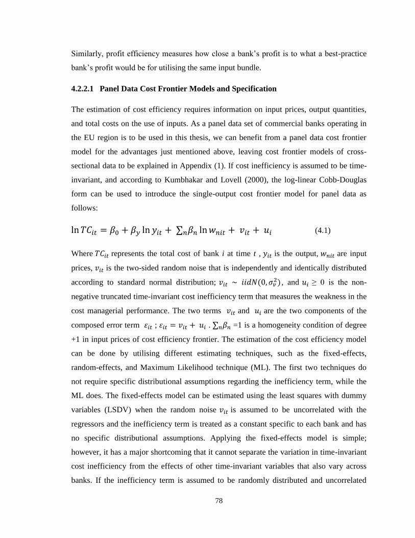
78

Similarly, profit efficiency measures how close a bank’s profit is to what a best-practice

bank’s profit would be for utilising the same input bundle.

4.2.2.1 Panel Data Cost Frontier Models and Specification

The estimation of cost efficiency requires information on input prices, output quantities,

and total costs on the use of inputs. As a panel data set of commercial banks operating in

the EU region is to be used in this thesis, we can benefit from a panel data cost frontier

model for the advantages just mentioned above, leaving cost frontier models of cross-

sectional data to be explained in Appendix (1). If cost inefficiency is assumed to be time-

invariant, and according to Kumbhakar and Lovell (2000), the log-linear Cobb-Douglas

form can be used to introduce the single-output cost frontier model for panel data as

follows:

(4.1)

Where represents the total cost of bank i at time t , is the output, are input

prices, is the two-sided random noise that is independently and identically distributed

according to standard normal distribution; ( ) , and ≥ 0 is the non-

negative truncated time-invariant cost inefficiency term that measures the weakness in the

cost managerial performance. The two terms and are the two components of the

composed error term ; . =1 is a homogeneity condition of degree

+1 in input prices of cost efficiency frontier. The estimation of the cost efficiency model

can be done by utilising different estimating techniques, such as the fixed-effects,

random-effects, and Maximum Likelihood technique (ML). The first two techniques do

not require specific distributional assumptions regarding the inefficiency term, while the

ML does. The fixed-effects model can be estimated using the least squares with dummy

variables (LSDV) when the random noise is assumed to be uncorrelated with the

regressors and the inefficiency term is treated as a constant specific to each bank and has

no specific distributional assumptions. Applying the fixed-effects model is simple;

however, it has a major shortcoming that it cannot separate the variation in time-invariant

cost inefficiency from the effects of other time-invariant variables that also vary across

banks. If the inefficiency term is assumed to be randomly distributed and uncorrelated

79

with the noise term and the regressors, then we turn to a random-effects model that can be

estimated by a two-step generalised least squares (GLS) method. In spite of the ability of

the random-effects model to account for time-invariant regressors, its main drawback is

that it requires, unlike the fixed-effects model, the inefficiency term be uncorrelated with

the regressors. One of the studies that utilises fixed-effects and random-effects model is

the one conducted by Maudos et al. (2002a), in which the authors adopted such models

along with the distribution-free approach (DFA) to estimate cost and profit efficiency of

banks in ten European Union countries. On the other hand, the Maximum Likelihood

estimation (MLE) is a more widely used technique in the banking efficiency studies in

spite of its need for strong distributional assumptions to work efficiently. The three main

distributional assumptions associated with the application of Maximum Likelihood

estimation (MLE) are:

(i) ( )

(ii) ( )

(iii) and are distributed independently of the regressors, and of each

other.

While Pitt and Lee (1981) benefit from the assumptions of Maximum Likelihood to apply

it to panel data efficiency study assuming half-normal distribution, Battese and Coelli

(1988) and Kumbhakar (1987) assume normal-truncated specification to be used in panel

data studies. Different studies seeking to find out which of the three techniques, fixed-

effects, random-effects, and Maximum Likelihood (ML), is preferred to the others have

been conducted, such as Gong and Sickles (1989), Gathon and Perelman (1992), Bauer et

al. (1993) and Bauer and Hancock (1993). These studies proved similar efficiency results,

meaning there is no consensus on what approach is preferred. However, according to

Kumbhakar and Lovell (2000), the MLE generates more efficient estimates by utilising

the distributional assumptions when the independence of factors and regressors matters,

and truly the MLE is the most widely used approach in European banking efficiency

studies. In any of these estimation models, the cost efficiency of bank i can be measured

by the ratio of the minimum cost ( ) necessary to produce that bank’s output and the

actual cost ( ):

80

( ) ( )

( ) ( ) ( ) ( ̂ ) ( )

To obtain an estimate for to be applied in the above equation so as to generate the cost

efficiency score of a bank i, the conditional mean of the inefficiency term can be used

given the composed error term , following Jondrow et al. (1982), where the

total variance is

. Another point estimator for cost efficiency was proposed

by Battese and Coelli (1988). [For more discussion on cost efficiency estimation models

and point estimators of cost efficiency, refer to Kumbhakar and Lovell (2000) and Coelli

et al. (2005)].

The single-output cost frontier model (4.1) introduced above allows for time-invariant

cost efficiency, meaning that cost efficiency is assumed to be constant over time and

differs across banks. However, different models were proposed to allow for cost

efficiency to vary over time in the panel data context. For instance, Cornwell, Schmidt,

and Sickles (CSS) (1990) and Kumbhakar (1990) were amongst the first to introduce

stochastic frontier models in which efficiency is allowed to vary over time as well as

across firms (banks). In this sense, we can rewrite the single-output cost frontier model

(4.1) for panel data as follows:

(4.3)

With the only difference between the two models being the cost inefficiency term is time-

variant. This model, again, can be estimated using fixed-effects, random-effects, or

Maximum Likelihood (ML) approaches. Lee and Schmidt (1993) suggest that can be

formulated as

( ) (4.4); where ( ) represents a set of time dummies , and the estimation

of inefficiency that can be applied in equation (4.2) can be obtained by:

{ ̂ ̂ } ( ̂ ̂ ) . Battese and Coelli (1992) suggest the following time-varying

81

efficiency model that can be estimated using maximum likelihood technique with

equations (4.3) and (4.4):

( ) { ( )} (4.5)

Where is the additional parameter that has to be estimated. The model satisfies the

conditions: (i) ( ) ≥ 0 and (ii) ( ) increases at an increasing rate when < 0, decreases

at an increasing rate when > 0, or remains constant when = 0. The cost frontier model

(4.3) takes the Cobb-Douglas functional form that accommodates single output; however,

to adopt a multiple-output cost frontier model, we need more flexible and efficient

functional form than the Cobb-Douglas form. The following section will introduce such a

flexible functional form that is more suitable to be used in this study where different input

prices and outputs of different commercial banks operating in the EU region are used.

Cost Efficiency Model Specification:

In spite of its simple application, the Cobb-Douglas functional form has some

shortcomings that might negatively affect the measurement of cost efficiency in this

study. Hesenkamp (1976) argues that the Cobb-Douglas functional form cannot maintain

the curvature condition of the output space in case of multiple-output cost frontier. In

addition, Coelli et al. (2005) refer to the idea that Cobb-Douglas form is less flexible than

other forms, such as the translog form, because it is a first-order flexible form compared

with the second-order flexible forms. Moreover, the Cobb-Douglas assumes that

elasticities are constant, and hence it cannot be applied efficiently in case of variable

elasticities. For these reasons and to obtain more robust cost efficiency estimates, the

translog (TL) cost function form is adopted in this panel data study.

The translog function form is one of the most widely used functional forms in banking

efficiency studies, and was first introduced by Christensen et al. (1971, 1973), and it is a

generalisation of the Cobb-Douglas functional form. The appropriateness and soundness

of using such functional form in our banking efficiency study can be summarised in three

advantages. First, it allows for multiple outputs while maintaining the curvature properties

of cost/profit functions. Secondly, it provides a second-order Taylor series approximation

to cost/profit frontier at the mean of the data. Thirdly, as Kumbhakar and Lovell (2000:

82

143) state, “it performs the basis of much of the empirical estimation and decomposition

of cost [or profit] efficiency based on a system of equations.” However, the translog (TL)

function form is not without drawbacks. First, the translog functional form can be

considered as a local approximation to cost/profit function and might perform poorly if

the behaviour of bank costs/profits is global (McAllister and McManus, 1993).

Furthermore, White (1980) argues that the least square of the translog polynomial might

be biased of the series enlargement and, also, this form is a local approximation. The other

widely used alternative functional form in banking efficiency studies is the Fourier-

flexible functional form. The Fourier-flexible (FF) functional form is a semi-

nonparametric approach and it is a global approximation that was first introduced by

Gallant (1981, 1982), and was discussed later by Elbadawi et al. (1983), Chalfant and

Gallant (1985), Eastwood and Gallant (1991), and Gallant and Souza (1991). It was used

in banking efficiency studies, such as Spong et al. (1995) and Berger et al. (1997).

Compared to the translog functional form, the Fourier-flexible (FF) functional form is

more complicated as it contains some trigonometric terms. There is no consensus on

which of these two methods generates better results; however, the translog (TL) functional

form is to be adopted in this thesis. First, as Hasan and Marton (2003) argue, the Fourier-

flexible (FF) functional form needs more truncations of data to be specified. Secondly,

according to Berger and Mester (1997), both functional forms generate similar efficiency

results and the difference in the estimated mean efficiency between the two forms is

insignificant, so both forms are substantially equivalent from an economic point of view.

The translog specification of cost function to be estimated in this study can be written as

follows:

83

(

) ∑

(

)

∑∑

(

) (

) ∑

( )

∑ ∑

( ) ( ) ∑∑

( ) (

)

( ) ∑

( ) ∑

(

)

( )

Where is bank total costs (interest and non-interest expenses), (k =1,…, 3)

represents outputs, (j =1,…, 3) stands for input prices. To impose linear input price

homogeneity, total costs, and input prices are normalised by the third input price (the

price of borrowed funds). is the two-sided random error that captures random

fluctuations, and is the non-negative cost inefficiency term that captures the degree of

weakness in managerial performance and it follows, in this study, a truncated normal

distribution (to be explained soon in this section). Cost efficiency is measured by

substituting the estimation of inefficiency term in the equation ( ̂ ) . The

cost function in equation (4.6) has to be linearly homogenous in input prices and for the

second-order parameters to be symmetric, so the following restrictions must be imposed:

∑

∑

∑

( )

The reason behind the inclusion of financial equity ratio EQ in the estimated cost function

is threefold. Berger and Mester (1997) argue that, first, managerial risk preference should

be accounted for in the cost function as bank managers differ from each other in term of

how risk-averse they are. More risk-averse managers will tend to maintain higher level of

equity than the cost-minimising level so as to absorb financial shocks, and therefore not

controlling for financial capital would penalise such risk-averse managers. Secondly, the

inclusion of equity capital helps in accounting for insolvency risk that affect bank costs

84

through the risk premium that must be paid for uninsured debt and through the extra costs

related to risk management activities. Thirdly, as an alternative fund to deposits, capital

level directly affects costs in the sense that interest paid on debt counts as a cost while

dividends paid do not. On the other hand, higher costs are associated with raising equity

than raising deposits meaning a negative effect of higher equity on costs. For these

reasons, it is objective to consider equity capital when measuring cost efficiency [see

Berger and Mester (1997), Mester (1996), Altunbas et al. (2000) and Mamatzakis et al.

(2008)].

Measuring bank efficiency in the method shown above does not provide answers as to the

causes of efficiency differences among banks and across countries. The answer to such

question, as argued by Berger and Mester (1997), is of some interest to public policy,

bank management, and banking studies. Different regulatory, bank-specific, industry-

specific, and macroeconomic factors might influence banking efficiency among banks

operating in different countries. The widely approach by which the effect of those factors

on bank efficiency can be measured is regressing in/efficiency against such variables. This

has been done in bank efficiency literature using two methods, the two-stage and one-

stage approaches.

According to the two-stage approach, bank in/efficiency estimates are generated in the

first stage using one or more of the efficiency techniques described above, and regress

such estimates against different efficiency correlates in the second stage. This approach

has been adopted by many efficiency studies, such as Allen and Rai (1996), Berger and

Hannan (1998), Bonin et al. (2005), Berger and Mester (1997) and Hasan and Marton

(2003). The two-stage approach has been criticised by Wang and Schmidt (2002) who

argue that the assumption that the inefficiency component is independently and identically

distributed across banks is violated in the second step of the approach, where the

inefficiency estimate is assumed to be dependent on different explanatory variables.

Therefore, according to the authors, the efficiency estimates generated in the first step are

biased and inconsistent. To overcome such criticism of the two-stage approach, a one-step

approach was introduced first by Kumbhakar et al. (1991), and was extended by Battese

and Coelli (1995) to allow for panel data. The Battese and Coelli (1995) model is adopted

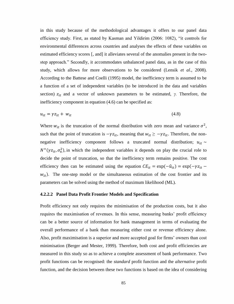
85

in this study because of the methodological advantages it offers to our panel data

efficiency study. First, as stated by Kasman and Yildirim (2006: 1082), “it controls for

environmental differences across countries and analyses the effects of these variables on

estimated efficiency scores [, and] it alleviates several of the anomalies present in the two-

step approach.” Secondly, it accommodates unbalanced panel data, as in the case of this

study, which allows for more observations to be considered (Lensik et al., 2008).

According to the Battese and Coelli (1995) model, the inefficiency term is assumed to be

a function of a set of independent variables (to be introduced in the data and variables

section) and a vector of unknown parameters to be estimated, γ. Therefore, the

inefficiency component in equation (4.6) can be specified as:

(4.8)

Where is the truncation of the normal distribution with zero mean and variance ,

such that the point of truncation is , meaning that ≥ . Therefore, the non-

negative inefficiency component follows a truncated normal distribution;

( ) in which the independent variables it depends on play the crucial role to

decide the point of truncation, so that the inefficiency term remains positive. The cost

efficiency then can be estimated using the equation ( ̂ ) (

) The one-step model or the simultaneous estimation of the cost frontier and its

parameters can be solved using the method of maximum likelihood (ML).

4.2.2.2 Panel Data Profit Frontier Models and Specification

Profit efficiency not only requires the minimisation of the production costs, but it also

requires the maximisation of revenues. In this sense, measuring banks’ profit efficiency

can be a better source of information for bank management in terms of evaluating the

overall performance of a bank than measuring either cost or revenue efficiency alone.

Also, profit maximisation is a superior and more accepted goal for firms’ owners than cost

minimisation (Berger and Mester, 1999). Therefore, both cost and profit efficiencies are

measured in this study so as to achieve a complete assessment of bank performance. Two

profit functions can be recognised: the standard profit function and the alternative profit

function, and the decision between these two functions is based on the idea of considering

86

market power or not. Berger and Mester (1997: 899) state that, “standard profit efficiency

measures how close a bank is to producing the maximum possible profit given a particular

level of input prices and output prices.” In other words, the standard profit function

assumes that the output markets are perfectly competitive so that banks are output price

takers. In contrast, the alternative (non-standard) profit function measures how close a

bank is to producing the maximum feasible profits given a particular level of input prices

and output quantities. According to the alternative profit function, banks are assumed to

have some market power in determining their output prices, or in other words, the

perfectly competitive output markets assumption cannot be held. Berger and Mester

(1997) argue that the alternative profit function is preferred over the standard profit

function when: (1) banking services are not at the same quality level; (2) the assumption

that output markets are perfectly competitive is questionable, so that banks have some

market power in deciding their output prices they like to charge. Since our sample in this

study includes a large set of commercial banks operating in 27 EU member states where

the level of competition in markets along with the quality of banking services are

different, then the alternative profit function is preferred and is adopted in this thesis. The

alternative profit function has been adopted in different European bank efficiency studies,

such as Hasan and Marton (2003), Hollo and Nagy (2006), Kasman and Yildirim (2006),

Yildirim and Philippatos (2007) and Mamatzakis et al. (2008).

The same analysis followed to introduce cost frontier models for panel data can be applied

for the profit frontier models. As a best-practice cost frontier has to be constructed, a best-

practice profit efficiency frontier has to be specified so that the relative profit efficiencies

of banks in the sample can be measured. In this sense, the alternative profit efficiency of

bank i can be measured by the ratio of the actual profit ( ) to the maximum feasible

profit ( ) that can be achieved by the best-practice banks:

( ) ( ) ( )

( ) ( ) ( ̂ ) ( )

The composed error in the profit efficiency case can be written as: , where

the inefficiency term has a negative sign because the inefficient banks obtain less profit

than the most efficient banks (operating on the profit frontier), and therefore, they deviate

87

negatively from the profit frontier. In other words, banks with lower are closer to the

most efficient banks located on the profit efficiency frontier, while banks with higher

can be found further from the profit frontier.

Profit Efficiency Model Specification

The profit efficiency function employs the same set of input prices, outputs, and

environmental variables, and hence it follows very similar translog specification as that of

cost efficiency’s and can be written as follows:

(

) ∑

(

)

∑∑

(

) (

) ∑

( )

∑ ∑

( ) ( ) ∑∑

( ) (

)

( ) ∑

( ) ∑

(

)

( )

Subject to:

∑

∑

∑

( )

Where the difference between model (4.6) and (4.10) is that the dependent variable in

model (4.10) is the bank pre-tax profit, where is a constant equals to one plus the

absolute value of minimum profits over all banks in the sample so as to allow for taking

logarithm of positive numbers and the inefficiency term has a negative sign23

. As in the

case of cost function model (4.6), the inefficiency term in equation (4.10) is dependent on

a set of environmental variables, and the maximum likelihood technique is used to

23

In adding this way, we follow Mamatzakis et al. (2008), Kasman and Yildirim (2006) and Yildirim and

Philippatos (2007).

88

estimate the parameters for the one-step Battese and Coelli (1995) profit efficiency model.

Profit efficiency scores can be generated using the equation ( ̂ ). In this

thesis all the frontier models are estimated using maximum likelihood technique based on

the computer software LIMDEP 10.24

4.3 Measuring Banking Risk

As illustrated in the literature section in this study, banking risk plays a strong influence

on banking performance and increases the possibility of facing serious turmoil by banks

maintaining high level of risk. Moreover, as highlighted, also, earlier in this study, one of

the main causes of the global financial crisis (2007-2009), was the increasing trend of

different banking risks by the time of the crisis. In this study, banking risk will be

analysed using descriptive statistics and illustrative figures for the entire period of the

study. This allows for investigating the trend of risk in European banking sector before

and during the time of the crisis. This banking risk investigation will be extended to

compare the level of risk maintained by the banking sectors in the two subsamples of the

new and old EU member states and also to shed light on the banking risk performance in

the GIIPS countries. The methodology adopted in this study for measuring banking risk is

financial ratios. Using financial ratios is a simple and practical method that generates

useful measurements, such as the mean, median, and standard deviation, to be analysed

using descriptive tables and figures. Moreover, and more importantly in this thesis, such

financial ratios can be used as explanatory variables in the one-step efficiency models to

investigate the effect of risk on banking cost and profit inefficiencies. In addition, such

financial ratios can assist in analysing the effect of risk on banking inefficiency during the

crisis time by utilising the interactive variables25

. Utilising the interaction between risk

variables and the world crisis dummy allows for taking the effect of global crisis upon the

bank risk-inefficiency relationship.

24

LIMDEP is econometric software developed by William H. Greene. 25

An interactive effect exists when the effect of one independent variable on a dependent variable differs

based on a third variable’s value (Jaccard, 2001).

89

As discussed in Chapter 2, there are different types of bank risks classified by authors,

however, in this thesis we descriptively analyse three types of risks; namely, insolvency

risk, credit risk and liquidity risk. The world financial crisis highlighted the importance of

these banking risks; hence, they are chosen based on the criterion of serving the objectives

of this study and whose data are available for such a large sample of banks operating in

the 27 EU states.

Insolvency risk is the risk that a bank might not be able to service its debts and hence

becomes insolvent (unable to satisfy its debts). In this sense, it is a long-term survival

issue that should encourage the bank to maintain higher level of capital so as to absorb

any unexpected shocks or market fluctuations, such as financial or economic crises.

Berger and Mester (1997) argue that a bank’s insolvency risk depends on its financial

capital available to absorb portfolio losses. Also, Rose (1999) argues that one of the

popular measures of insolvency risk is the ratio of capital to total assets. Therefore, to

measure insolvency risk the well-known financial capital ratio (or equity ratio) is used in

this study. The ratio of equity to total assets as a measure of insolvency risk is very

common in banking efficiency and risk studies and is used in many of them, such as Allen

and Rai (1996), Yildirim and Philippatos (2007), Hasan and Marton (2003), Lozano-

Vivas et al. (2002) and Fiordelisi et al. (2011).

Credit risk can be defined as the probability that the value of some of the bank’s assets,

particularly loans, would depreciate as some of the bank’s borrowers might fail to meet

their obligations, such as default on their loans (Rose, 1999). The financial ratio used to

measure credit risk in this study is the non-performing loans to gross loans ratio. This

ratio as a measure of credit risk is widely used in banking efficiency and risk studies,

among those studies are Fries and Taci (2005), Berger and DeYoung (1997), Altunbas et

al. (2000) and Fiordelisi et al. (2011).

Finally, liquidity risk can be expressed as the risk that a bank is not able to meet its

financial obligations, such as deposit withdrawals, net loan demand, and other cash

requirements as they come due because it does not have sufficient cash or borrowing

capacity at that time (Rose, 1999). An illiquid bank might be forced to borrow emergency

cash at a higher interest rate or pay a higher interest rate on issued securities to meet

90

unexpected events, therefore committing more costs and generating less profit. To

measure liquidity risk, the ratio of total loans to total assets is used, as the higher the ratio

of loans indicates less liquidity position. This measure is used in different studies, such as

Yildirim and Philippatos (2007), Havrylchyk (2006), Maudos et al. (2002a), Allen and

Rai (1996) and Altunbas et al. (2000).

4.4 Data Description and Variables

4.4.1 Bank Efficiency and its Determinants

The first objective of this thesis is to measure cost and profit efficiencies and to

investigate their relationship with risk and other factors in the 27 banking systems of the

European Union member states over the period 2004-2010. The large sample of 27 EU

countries is to be further divided into three sub-samples; namely the new EU countries

(Bulgaria, Cyprus, Czech Republic, Estonia, Hungary, Latvia, Lithuania, Malta, Poland,

Romania, Slovakia, and Slovenia), the old EU countries (Austria, Belgium, Denmark,

Finland, France, Germany, Greece, Ireland, Italy, Luxembourg, Netherlands, Portugal,

Spain, Sweden, and the United Kingdom)26

, and the GIIPS countries (Greece, Ireland,

Italy, Portugal, Spain). This sub-sampling allows for comparing banking efficiency and

risk between the old and the new EU states as well as highlighting bank efficiency and

risk for the GIIPS countries that have faced sovereign debt crises as a reflection of the

recent global crisis 2007-2009. The study period of 2004-2010 is of particular importance

as it covers the period where 12 of the new EU countries joined the European Union after

transitional period in addition to the recent global financial crisis time 2007-200927

.

The data used to measure bank efficiency and its determinants are collected from balance

sheets and income statements of commercial banks provided by “Bankscope” database of

BVD-IBCA, and according to Mathieson and Roldos (2001), Bankscope has good

26

In this thesis, and following studies, such as Hollo and Nagy (2006), Kosak et al. (2009), and Mamatzakis

et al. (2008), we define the new EU countries as the 12 member states that joined the European Union in

2004 and 2007, while the old EU countries are the 15 states that completed their membership before 2004. 27

Croatia is excluded from the EU sample as it joined the EU in 2013; the year which is beyond the time

period of our study (2004-2010).

91

advantages. In addition to its broad coverage of banks whose total assets account for 90%

of total assets in each country, it allows for logical comparisons between banks and

countries as it adjusts all the collected data in one compatible global format.

Macroeconomic data, on the other hand, are collected from “Datastream” database

developed by Thomson Financial Limited and from the IMF’s International Financial

Statistics. All data are collected in US dollars rather than euros or local currencies, and

therefore data are directly corrected for inflation. According to the Purchasing Power

Parity theory (PPP), in general, a country with a lower inflation rate will have a rising

currency value that would be reflected by the exchange rate (Mankiw, 2011). Also, Isik

and Hassan (2003) argue that the relative version of PPP theory states that the exchange

rate between two countries will adjust to reflect changes in the price levels of the two

countries. Hence, as data are transformed from the original country currency to the US

dollar, then data in this study are corrected for inflation. Using the US dollar to collect

data from the 27 countries not only help correcting for inflation but also use a single

currency to collect data rather than using different local currencies along with the euro to

bring the data in a homogenous format. The focus for measuring efficiency and risk in this

thesis is on commercial banks only so as to maintain the homogeneity in such large

sample that includes 27 countries and make the comparison between the new and old EU

states more logical. We use a sample consisting of unbalanced panel dataset composed of

4250 observations corresponding to 947 commercial banks operating in the 27 EU states,

after removing 533 banks whose dependent or independent variables were not available28

in addition to some outliers, over the period 2004-2010. The sample is restricted to

commercial banks whose control and environmental variables are available.

Unsurprisingly, the number of commercial banks included in the study sample from the

old EU states (745 banks) dominates the number of banks from the new EU states (202

banks). Regarding the GIIPS countries, 202 commercial banks operating in these

countries are included in the sample, and Appendix 2a summarises the number of banks

and observations for each country over the period 2004-2010. From the sample explained

28

As an exception, banks whose non-performing loans/gross loans ratios are not available where not

removed because removing such banks would significantly shrink and deteriorate our sample, and how to

deal with this issue will be explained later in this study.

92

above, we create a sub-sample of only listed commercial banks for which we have data on

the determinants of stock returns, as to be explained in Chapter 7.

Variables Specification and Definition

4.4.1.1 The Input and Output Variables (Control Variables)

A big challenge that is faced by banking efficiency studies is the definition and

measurement of inputs and outputs and, unfortunately, there is no consensus on such

issue. To specify the input prices and outputs to be used in equations (4.6) and (4.10), two

main approaches have been suggested in the literature; namely, the “production approach”

and the “intermediation approach”29

. Under the production approach, banks are

considered as mainly producing services for account holders (Berger and Humphrey,

1997), and therefore, physical inputs, such as labour and capital are used to produce bank

outputs, such as deposits, loans and other bank liabilities. On the other hand, under the

intermediation approach, proposed by Sealey and Lindley (1977), banks are thought of as

financial intermediaries that channel funds between savers and investors, and hence

deposits, other borrowed funds, capital, and labour are considered as inputs transferred in

the production process into outputs, such as loans and other earning assets. While Berger

and Humphrey (1997) point out that the production approach is somewhat better for

evaluating the efficiency of branches of financial institutions, they argue that the

intermediation approach might be more appropriate for evaluating the efficiencies of

entire financial institutions. Following modern empirical literature on bank efficiency;

such as Hollo and Nagy (2006), Mamatzakis et al. (2008) and Altunbas et al. (2001), the

empirical analysis in this thesis adopts the intermediation approach.

Therefore, according to the intermediation approach, we define input prices as the price of

labour, the price of physical capital, and the price of borrowed funds. Our outputs are

total loans, other earning assets, and off-balance sheet items. Even though off-balance

sheet items are technically not earning assets, the importance of such items as a source for

29

There is also the value-added approach proposed by Berger and Humphrey (1992), for more, see Berger

and Humphrey (1992).

93

generating income for banks has been increasing in recent years, and therefore they

should be included in cost and profit functions (Jagtiani and Khanthavit, 1996). Among

the studies that include off-balance sheet items in the efficiency function are Altunbas et

al. (2001a), Carbo et al. (2002), Havrylchyk (2006) and Altunbas et al. (2001b). Finally,

as mentioned earlier in the methodology section, the left-hand side of the cost function is

the bank total costs, and the left-hand side of the profit function is the bank pre-tax profit,

and total costs, pre-tax profit, and the input prices are normalised by the price of borrowed

funds. The following table summarises cost and profit functions main variables along with

their description:

Table 4.1. Input and Output Variables

Variable Symbol Name Description

Dependent

Variables

TC Total Costs Total interest and non-interest expenses

π Profit Pre-tax profit

Input

Prices

w1 Price of labour Personnel expenses/total assets*

w2 Price of physical capital Other operating expenses(non-interest expenses

less personnel expenses)/fixed assets

w3 Price of borrowed funds total interest expenses/total funding

Outputs

y1 Total loans Sum of short- and long-term loans

y2 Other earning assets Total earning assets less total loans

y3 Off-balance sheet items Total off-balance sheet items

Other

Variables EQ Equity ratio Equity capital as a proportion of total assets

* We divide personnel expenses by total assets instead because Bankscope does not provide information on the

number of employees.

Table 4.2 displays summary statistics for the dependent variables, input prices, outputs

and equity ratio that are used in the cost and profit efficiency functions. The table is

divided into four samples that represent the entire EU region (EU27), the old EU countries

(EU15), the new EU countries (EU12), and the GIIPS countries (EUGIIPS). As can be

seen from the table, the mean prices of labour, physical capital, and borrowed funds for

the entire EU region are (1.38%), (440.56%), and (2.89%), respectively, while the mean

equity ratio stands at 8.90%. The mean prices of labour and borrowed funds are higher for

banks in the new EU countries than those in the old EU countries, while the mean prices

94

of physical capital is significantly much higher for banks in the old EU countries. This

might be attributed to the idea that commercial banks in the old EU states substitute

physical capital for labour while banks in the new EU states prefer to use labour. On the

other hand, it appears from the table that over the seven years of our study period

commercial banks operating in the old EU states maintain higher insolvency risk on

average (equity ratio of 8.59%) than the banks in the new EU states (equity ratio of

10.04%). Regarding the GIIPS countries, the table shows that the prices of labour,

physical capital and borrowed funds are lower, on average, than they are in all the old EU

countries, while the equity ratio is higher (at 9.32%). Moreover, the mean price of

physical capital is lower and the equity ratio is higher for the new EU countries than the

GIIPS countries. Finally, it can be noticed that total costs of banks in the new countries

are much lower than those in the old countries, though the pre-tax profits are similar in

values between the two groups. It can be said here that commercial banks in the old EU

countries spend more on technology and fixed assets as well as other expenses as banks

might be larger in the old countries. On the other hand, even though total loans in the new

EU countries is lower in value than they are in the old countries, banks in the new

countries might generate high profits as the markets there might be less competitive

allowing banks to impose higher interest rates on loans and also might generate

substantial profits from activities other than lending.

95

Table 4.2. Descriptive Statistics of Dependent Variables, Input Prices and Outputs (2004-2010)

Country

Sample Statistics

Dependent

Variables Input Prices Outputs Others

Total

Costs

(TC)

Pre-tax

Profit

(π)

Price

of

Labour

(w1) %

Price of

Physical

Capital

(w2) %

Price of

Borrowed

Funds

(w3) %

Total

Loans

(y1)

Other

Earning

Assets

(y2)

Off-

balance

Sheet

(y3)

Equity

Ratio

(EQ) %

EU

27

Obs 4250 4250 4250 4250 4250 4250 4250 4250 4250

Mean 1555.352 25957.64 1.38378 440.5642 2.88544 19314.13 21900.85 9810.643 8.904146

Std.Dev 7069.024 1453.95 1.28056 1191.002 2.64469 82502.18 127599.3 66043.38 7.01275

Min 29.411 -309296 0.004 2.193 0.260 0.623 0.79 0.996 0.100

Max 808014 3564748 5.171 670.212 6.731 1113372 2449260 3061809 75.2

EU

15

Obs 3322 3322 3322 3322 3322 3322 3322 3322 3322

Mean 1921.987 25989.58 1.37731 512.1451 2.80755 23918.32 27588.56 12275.13 8.585647

Std.Dev 7954.552 1640.722 1.36373 1329.414 2.83927 92762.19 143805.6 74508.51 7.22214

Min 29.411 -309296 0.004 4.224 0.260 2.211 1.300 1.025 0.110

Max 808014 3564748 5.171 670.212 6.731 1113372 2449260 3061809 75.2

EU

12

Obs 928 928 928 928 928 928 928 928 928

Mean 242.8944 25843.28 1.40693 184.323 3.16425 2832.33 1540.301 988.3998 10.04429

Std.Dev 397.1612 169.7118 0.92358 293.489 1.75482 4888.007 3254.277 2072.892 6.073602

Min 31.002 -116794 0.02 2.193 0.943 0.623 0.79 0.996 0.100

Max 13326 304222 4.23 390.200 5.992 242171 224510 26691 68.9

EU

GIIP

S

Obs 797 797 797 797 797 797 797 797 797

Mean 1510.04 26014.99 1.2782 465.7065 2.34098 23886.28 11143.67 8042.482 9.321405

Std.Dev 5480.222 1844.107 0.91238 1571.826 1.35118 77956.47 39489.51 30592.13 7.968401

Min 85.412 -309296 0.004 3.551 0.347 1.000 0.88 1.000 0.200

Max 274335 3151240 4.23 592.110 4.211 994527 1051720 1944430 73.3

Note: All values are in millions of US$, except where indicated.

4.4.1.2 The Environmental Variables (Efficiency Correlates)

Even though the integration between the 27 EU states, particularly between the new and

old EU states, has strengthened during the last decade as a result of economic

convergence and harmonisation introduced by the “Acquis Communautaire”, there still

exist differences in the macroeconomic and regulatory environment (Hollo and Nagy,

2006). Without taking such differences, that are out of the control of bank management,

into account, differences in cost and profit efficiencies among banks and across countries

would be fully attributed to the bank managerial decisions, which might not be the case.

96

So, it is crucial to investigate different bank efficiency correlates that might help in

explaining differences in efficiency (or inefficiency) between banks and across countries,

which might provide important implications for public policy, research and bank

management (Berger and Mester, 1997). These variables are not generally controlled by

bank management, or at least are partially exogenous. As explained earlier in equation

(4.8), the inefficiency component will be regressed in the one-step model, according to

Battese and Coelli (1995), against different efficiency correlates (independent variables).

In this thesis, we divide the explanatory (independent) variables into two groups, banking

risk variables and other explanatory variables. While the first group includes the three risk

variables discussed above and their interaction with the crisis variable, the latter group

include different bank specific, industry, and macroeconomic variables. We define the

variables in each group as follows:

1. Banking Risk Variables

Equity Ratio (Insolvency Risk)

This ratio measures the financial insolvency risk of a bank and is calculated as the ratio of

equity capital to total assets. Berger and Mester (1997) argue that insolvency risk

influences costs and profits of banks through the higher risk premium that has to be paid

by banks to borrow and through the costs involved with risk management activities, in

which case equity ratio should have a negative effect on bank cost and profit

inefficiencies. However, the direction of the effect of this variable might be the reverse as

raising capital is more expensive than debt or if the moral hazard hypothesis, where banks

with low solvency position would undertake risky business to compensate, holds.

Therefore, we do not have a prior expectation for the influence of equity ratio on cost and

profit inefficiencies. A negative correlation between capital and inefficiency is confirmed

by Fries and Taci (2005), Yildirim and Philippatos (2007), and Grigorian and Manole

(2002). On the other hand, a positive correlation between bank inefficiency and equity

97

ratio is observed by Altunbas et al. (2007), Allen and Rai (1996) and Hasan and Marton

(2003), suggesting that risk-averse banks are associated with lower efficiency.

Equity Ratio * Crisis

As explained in the literature earlier in this thesis, the level of risk maintained by banks

played a key role in the global financial crisis 2007-2009. Part of that risk was enhanced

by high level of financial leverage (low level of equity ratio) maintained by banks by the

time of the world crisis. To shed light on the nature of the correlation between bank

inefficiency and insolvency risk during the global crisis time and how the crisis affected

such a relationship, we create an interactive variable between the equity ratio and the

dummy variable of the world financial crisis 2007-2009 (the crisis dummy to be explained

later). The expected sign of this variable is negative regarding both cost and profit

inefficiency, suggesting that commercial banks with higher capital ratio are more efficient

as they are more capable of surviving the negative effects of the crisis than less capitalised

banks.

Total Loans/Total Assets (Liquidity Risk)

This ratio can be considered as a liquidity ratio with higher total net loans/total assets ratio

meaning less liquidity position for a bank as loans are among the most illiquid assets. This

ratio is of particular interest as an illiquid bank might face an emergency borrowing at

higher interest rate to meet its obligations, and even worse, an illiquid bank might face

bank runs30

forcing it to fail even though it might be solvent. In this sense, this liquidity

ratio is expected to have a positive effect on bank cost inefficiency; however, an adverse

effect is confirmed by studies, such as Yildirim and Philippatos (2007) and Allen and Rai

(1996). Regarding profit inefficiency, total loans/total assets ratio is expected to influence

profit inefficiency negatively as a higher risky position is correlated with higher profits,

and also the return on loans is higher than the return on liquid assets, such as government

securities. Yildirim and Philippatos (2007) and Maudos et al. (2002a), find no significant

relationship between profit inefficiency and loans-to-assets ratio.

30

Bank run is the situation when a large number of a bank’s clients withdraw their money (or deposits)

because of their concerns about the solvency issue of the banks, which might force the bank to go bankrupt

as a result.

98

Total Loans/Total Assets * Crisis

It is interesting to shed light on the effect of the world crisis 2007-2009 on the relationship

between liquidity risk and bank inefficiency. In other words, a question of interest is to

what extent the liquidity risk affects bank cost and profit inefficiencies during the crisis

time. To answer this question, an interactive variable is created between liquidity risk and

the dummy variable of the world financial crisis 2007-2009, as in the case of equity ratio

and the crisis interactive variable. This variable is expected to have a positive effect on

cost and profit inefficiencies as banks with higher liquidity might have decreased the costs

of emergency borrowing and the costs of losses associated with default loans in the credit

crunch state during the crisis time.

Non-Performing Loans/Gross Loans (Credit Risk)

One good measure of bank credit risk is the ratio of non-performing loans to total loans

that reflects potential losses for a bank. The International Monetary Fund defines a non-

performing loan as follows: “A loan is non-performing when payments of interest and

principal are past due by 90 days or more, or at least 90 days of interest payments have

been capitalized, refinanced or delayed by agreement, or payments are less than 90 days

overdue, but there are other good reasons to doubt that payments will be made in full.”31

The higher the ratio of the non-performing loans to total loans is, the more risky a bank is,

which in turn might affect the bank inefficiency. As the percentage of non-performing

loans increases, the bank costs related to monitoring, working out, or selling off bad loans

increase, and therefore, this variable is expected to positively affect cost inefficiency.

Berger and DeYoung (1997), Fries and Taci (2005), and Altunbas et al. (2000) find non-

performing loans to total loans ratio to be positively correlated with bank cost

inefficiency. Similarly, this variable is expected to be positively associated with bank

profit inefficiency as it would increase costs and expenses related to the loan-loss

provision32

in the income statement, which in turn reduces a bank’s net income (profits).

It is important to refer here that regarding this variable and due to missing data, we will

31

In Bloem and Freeman (2005), p. 2. 32

Loan-loss provision is an expense set aside to account for possible losses on loan defaults.

99

run a separate regression model and include only the observations for which data of this

variable are available.

Non-Performing Loans/Gross Loans * Crisis

As explained in the literature above on the causes of the world crisis, the credit risk was

increased at financial institutions due to different reasons. To see what role the credit risk

played in terms of bank cost and profit inefficiencies during the crisis time, we create

interactive variables between the ratio of non-performing loans to total loans and the

dummy variable of the world crisis 2007-2009. For the reasons mentioned above, we

expect that bank cost and profit inefficiencies are positively correlated with the level of

non-performing loans to total loans during the crisis time.

2- Other Explanatory Variables

Size

Bank size is measured by taking the logarithm of total bank assets measured in millions of

US dollars to account for a possible non-linear relationship between bank inefficiency and

size. Bank size is expected to affect negatively both cost and profit inefficiencies,

meaning that larger banks are expected to be more cost and profit efficient probably due

to, as Yildirim and Philippatos (2007: 138) refer, “the relaxation of asset restrictions in the

banking system that [allows] banks to grow and venture into different banking business

practices, and to accrue some economies of scale and scope.” The expected positive

relationship between size and efficiency could also be attributed to the higher ability of

large banks to attract and retain better bank managers, as discussed by De Young and

Nolle (1998). Although we expect a positive relationship between bank size and

efficiency, this relationship might be negative. Isik and Hassan (2002) argue that the

overhead costs of small banks might be low because they often operate few branches

compared to larger banks, so they may possess operational advantage which might results

in higher efficiency. Also, larger banks might issue loans to a larger number of people and

in small amount, which in turn might increase the costs of servicing and monitoring

100

leading to lower efficiency. Size has been used enormously in bank efficiency studies and

has been found to have a negative effect on bank inefficiency in studies, such as Hasan

and Marton (2003), Yildirim and Philippatos (2007), and Matousek and Taci (2004),

while the reverse is found by Bonin et al. (2005) and Allen and Rai (1996).

Return on Average Assets (ROAA)

ROAA is a proxy used to assess the profitability of a bank’s assets and is calculated by

dividing the net income by the average total assets. ROAA is a bank performance measure

and is expected to be negatively correlated with bank cost and profit inefficiencies. Chan

and Abd Karim (2010) in their study on bank cost and profit efficiency in developing

countries find a negative relationship between bank profit inefficiency and the return on

assets meaning better utilisation of assets enhances bank profit efficiency. Carbo et al.

(2002) and Lensik et al. (2008) find this variable to have a negative effect on bank cost

inefficiency, while Matousek and Taci (2004) find it to positively affect bank inefficiency.

Intermediation Ratio

Intermediation ratio represents the overall depth of bank intermediation activity and

reflects the ability of banks to convert deposits into loans, and is calculated by dividing

total loans by total deposits. This variable is expected to negatively influence bank

inefficiency because higher intermediation ratio means less deposits are required to

produce loans, which in turn means lower production costs and hence higher profits.

Kosak et al. (2009), Fries and Taci (2005), and Dietsch and Lozano-Vivas (2000) find the

expected negative relationship between intermediation ratio and bank cost inefficiency.

Market Concentration

Market concentration is calculated as the sum of total assets of the five largest banks

divided by the total assets of the entire banking system. There are two main hypotheses

that explain the relationship between market concentration and efficiency. Structure-

Conduct-Performance (SCP) hypothesis assumes that a higher bank concentration allows

a higher degree of cooperation between them. These banks might set higher prices and

consequently gain substantial profits [see Heffernan (1996) and Molyneux et al., (1996)].

101

On the other hand, the Efficiency-Structure (ES) hypothesis suggests that a bank which

operates more efficiently than its competitors gains higher profits resulting from low

operational costs and holds an important share of the market [see Demsetz (1973) and

Berger (1995)].

Banks operating in a more concentrated market, where the level of competition might be

lower, are expected to have greater market power and therefore charge higher prices and

generate more profits. In this sense, we expect that higher concentration ratio is correlated

negatively with bank profit inefficiency, as it is confirmed by Maudos et al. (2002a). In

terms of cost inefficiency, the concentration ratio might affect negatively cost inefficiency

if concentration is a consequence of a better management or implementing the production

process more efficiently (Demsetz, 1973). On the other hand, if concentration is a result of

market power, then that would induce banks to spend more on staff and other personnel

expenses (Leibenstein, 1966), or banks would feel less pressure to control their costs, and

therefore concentration ratio would have a positive influence upon cost inefficiency.

Therefore, we do not have specific sign for the relationship between bank cost

inefficiency and market concentration ratio, which could be positive or negative. Dietsch

and Lozano-Vivas (2000), Fries and Taci (2005), and Kosak et al. (2009) find positive

linkage between cost inefficiency and market concentration, while Maudos et al. (2002a)

find this linkage to be negative.

Inflation Rate

A macroeconomic variable that might have a potential effect on bank cost and profit

inefficiency which is to be investigated in this study, is inflation rate. Grigorian and

Manole (2002) argue that inflation might have a positive correlation with bank

inefficiency as excessive branch networks are often associated with high inflationary

environment. Hanson and Rocha (1986) argue that inflation increases bank costs as large

number of transactions might be associated with higher labour costs causing higher ratio

of bank branches per capita. In addition, an increase in inflation rate might increase

interest rates which might lead to higher costs faced by banks. Revell (1979) argues that

the impact of inflation on bank costs and profits depends on the rate at which operating

expenses increased as opposed to the inflation rate. Athanasoglou et al. (2006) suggest

102

that the influence of inflation on bank profits depends on how capable a bank is to

forecast inflation so as to bank managements handle their expenses and their interest rates

in order to generate profits. In this sense, if commercial banks have the ability to

successfully forecast changes in inflation rate, then that would positively affect bank

profitability. In our study where our sample contain banks operate in 27 countries, we do

not have the expected signs, either in terms of the effect of inflation on bank cost

inefficiency or on bank profit inefficiency. However, Weill (2003a) and Grigorian and

Manole (2002) find no significant relationship between inflation and bank inefficiency,

while Tomova (2005) finds a positive impact of inflation on bank technical efficiency.

Nominal Interest Rate

We use the long-term government bond yield provided by “Datastream” database to

represent this variable. The change in interest rate might affect bank costs and profits in

different directions. As Rose (1999) argues, an increase in market interest rate would raise

bank profits if a bank maintains an excess of flexible-rate assets over flexible-rate

liabilities, and would increase bank costs and decrease bank profits in the reverse

situation. Unless banks are hedged against interest rate movements, they might face high

losses and costs, and hence lower profits. However, higher interest rates might increase

bank interest costs and increase inefficiency in risk management and credit evaluation

through greater ambiguity and risk. Therefore, we would expect a positive relationship

between nominal interest rate and bank cost inefficiency, as found by Fries and Taci

(2005), but we do not have an expected sign in the case of profit inefficiency.

World Financial Crisis (2007-200933

)

As financial markets have become globally more integrated due to the world economic

globalisation, it was not possible for the European Union banking system to isolate itself

against a possible financial and banking contagion of the recent financial crisis that

originated in the United States. To investigate the effect of the world financial crisis on

the inefficiency of the commercial banking system in the EU, we construct a dummy

33

In this study we focus on potential contagion of the global financial crisis 2007-2009 that originated in the

US, therefore we consider the years from 2007 to 2009 as the period of the crisis following studies, such as

Eubanks (2010b) and Mishkin and Eakins (2012).

103

variable which takes the value of 1 for the years 2007-2009, and 0 otherwise. We would

expect that the world crisis affects both bank cost and profit inefficiency positively,

meaning that it might have reduced banks’ profits and increased banks’ costs as a result of

the economic turmoil and recession the crisis led to in the EU region. Banks might have

faced higher costs related to; first, expensive borrowing in a credit crunch environment,

second, raising capital (deleveraging), and third, monitoring and evaluating the

creditworthiness of clients, leading to more expenses associated with risk management at

the crisis time. On the other hand, banks’ profits are also expected to be affected

negatively by the crisis because of; first, lower lending activity followed by deposits

withdrawal and low liquidity, second, the losses associated with the loan defaults and

other assets over the crisis period, and third the increase in bank costs, as just explained

above, that leads to lower profits.

Country Dummy

In this study we tend to make a comparison between bank cost and profit efficiencies in

the old and new EU member states to see in which area banks operate more efficiently.

We investigate such difference by including a dummy variable that takes the value of 1 if

a bank operates in the old EU states and 0 if a bank operates in the new EU states. As

banks in the new EU states had to meet different criteria related to economic and political

reforms and financial requirements, we would expect that cost and profit efficiency of

commercial banks in such countries have continued to increase, at least in the early years

of the time period we consider in this thesis. However, we still believe that commercial

banks in the new EU states could not fully catch up or exceed the cost efficiency level of

banks in the old EU states due to the higher level of competition and technological

development and the better management techniques the old countries maintain in their

banking and financial markets. In this sense, we would expect the country effect variable

to have a negative effect on bank cost inefficiency, while we have no expectation with

regard to profit inefficiency as banks in the new EU countries might benefit from less

competitive environment to make some monopolistic profits and hence appear more profit

efficient.

104

Country Dummy * Crisis

To investigate whether bank cost and profit inefficiencies were affected more by the

world crisis and in what direction in the old or in the new EU countries; we create an

interactive variable between the country effect dummy variable and the world crisis

dummy variable. Because of the more integrated financial markets and institutions

between the old EU states and the US, and because financial institutions were more

involved in investing in the US mortgage toxic securities and other financial instrument in

the US than those in the new EU countries, we would expect this variable to have a

positive influence on both bank cost and profit inefficiency. This means that cost and

profit efficiencies of commercial banks in the old EU member states might have been

negatively more affected by the crisis than their counterparts in the new EU states.

GIIPS-Dummy

To investigate whether banks operating in the GIIPS countries differs from banks

operating in the other EU countries in terms of cost and profit efficiencies, we create a

dummy variable that takes the value of 1 for banks operating in these five countries, or 0

otherwise. As the sovereign debt crises started after the occurrence of the world financial

crisis, and since our time period covers from 2004-2010, we do not really have

expectations as to the effect of such a dummy variable on bank cost and profit

inefficiency.

GIIPS-Dummy * Crisis

To find out whether the world crisis affected cost and profit efficiencies of banks that

operate in the GIIPS countries more or less than banks operating in the rest of the EU

states, we construct an interactive variable between GIIPS-Dummy variable and the world

crisis dummy variable. Again, we do not have expectations as to the effect of such a

dummy variable on bank cost and profit inefficiency.

Appendix 2b summarises the explanatory variables stated above along with their

description, and the expected sign of their effects on bank cost and profit inefficiency.

105

Furthermore, Appendix 2c provides descriptive statistics for all the aforementioned

environmental variables.


This chapter summarises the methodological approaches that are used to estimate cost and

profit efficiencies in the European Union banking system over the period from 2004 until

2010. We employ the stochastic frontier analysis (SFA) and the Battese and Coelli (1995)

model to measure bank cost and profit efficiencies and investigate their determinants. This

chapter outlines the specifications of translog cost and profit frontier functions for panel

data based on the Battese and Coelli (1995) one-step model. It also highlights the financial

ratios adopted to measure insolvency, credit and liquidity risks at the EU commercial

banks. Furthermore, this chapter describes the dataset and variables used for the empirical

analysis which include the input and output variables as well as the determinants of bank

efficiency (efficiency correlates). We use a sample consisting of an unbalanced panel

dataset composed of 4250 observations corresponding to 947 commercial banks operating

in the EU countries over the period 2004-2010. The intermediation approach is followed

to specify the input and output variables for the efficiency functions. The efficiency

correlates, in turn, are divided into two groups; the first group represents bank risk

variables, while the second group represents the explanatory variables. The definitions,

descriptions and expected signs of these variables are also discussed in this chapter.

106

Chapter 5

Empirical Analysis of Efficiency in the European Union

Banking Sector

5.1 Introduction

This chapter analyses the efficiency of the European Union banking system for the years

from 2004 to 2010. Using the stochastic frontier approach based on the Battese and Coelli

(1995) model, cost and profit efficiencies scores are generated for four EU samples. This

chapter aims further to investigate and compare cost and profit efficiency levels based on

a common frontier, that pools together all the EU commercial banks used in this study,

and based on separate efficiency frontiers. The evolution and dispersion of the EU bank

efficiencies over time are investigated along with the efficiency gap between the old and

the new EU members. Also, this chapter indicates in what way the level of bank

efficiencies during the world financial crisis 2007-2009 is affected. Therefore, this chapter

addresses the first research question in this thesis.

The rest of this chapter is organised as follows: Section 5.2 reports the maximum

likelihood parameter estimates for the stochastic translog cost and profit functions.

Section 5.3 introduces the empirical results of cost and profit efficiency mean estimates

for the four sub-samples based on a comparison between the common frontier and the

separate frontiers. In addition, the mean efficiency scores for all the 27 EU countries and

the efficiency gap between the old and the new EU states as well as efficiency levels by

size groups are analysed based on the common frontier in Section 5.3. Section 5.4

discusses the evolution of bank cost and profit efficiencies for the individual EU countries

and the four sub-samples in addition to the evolution of efficiency gap between the old

and the new EU member states over the period 2004-2010 based on the common frontier.

Section 5.5 investigates the dispersion (heterogeneity) of bank cost and profit efficiencies

over time and within the four groups of the EU member states. In Section 5.6 we examine

107

the influence of the global financial crisis on cost and profit efficiency levels for all the

four sub-samples by comparing the mean efficiency scores in the crisis, the non-crisis, and

in the entire time period under study. Section 5.7 provides summary and conclusion.

5.2 Efficiency Frontier Estimates

5.2.1 Cost Frontier Estimates

The stochastic frontier models are used to estimate cost efficiency of 947 commercial

banks operating in the 27 European Union member states over the period 2004-2010.

Table 5.1 summarises the maximum likelihood estimates of parameters of the translog

cost function based on the SFA and the Battese and Coelli (1995) truncated normal

distribution.

108

Table 5.1 Maximum Likelihood Estimates for Cost Function Models

Variables Parameters Common

Frontier Separate Frontiers

Model 1 (EU27)

Model 2 (EU15)

Model 3 (EU12)

Model 4 (EUGIIPS)

Constant β0 8.116***

(0.0079)

8.1157***

(0.0088)

8.2465***

(0.0147)

8.17424***

(0.0149)

ln(W1/W3) χ1 0.4448***

(0.0026)

0.4454***

(0.0029)

0.4816***

(0.0111)

0.4783***

(0.0067)

ln(W2/W3) χ2 0.0482***

(0.0016)

0.0498***

(0.0018)

0.0539***

(0.0077)

0.0259***

(0.0052)

0.5ln(W1/W3)ln(W1/W3) δ11 0.1404***

(0.0024)

0.1435***

(0.0026)

0.1916***

(0.0142)

0.1341***

(0.0055)

0.5ln(W2/W3)ln(W2/W3) δ22 0.0050***

(0.0012)

0.0071***

(0.0013)

-0.0010

(0.0065)

0.0027

(0.0040)

ln(W1/W3)ln(W2/W3) δ12 0.0086***

(0.0014)

0.0054***

(0.0016)

0.0295***

(0.0055)

0.0058

(0.0041)

lnY1 β1 0.6917***

(0.0039)

0.6927***

(0.0043)

0.6495***

(0.0123)

0.6775***

(0.0083)

lnY2 β2 0.2642***

(0.0042)

0.2715***

(0.0048)

0.3101***

(0.0108)

0.2882***

(0.0095)

lnY3 β3 0.0064**

(0.0027)

0.0029

(0.0029)

0.0199**

(0.0096)

0.0079

(0.0064)

0.5lnY1lnY1 φ11 0.1282***

(0.0012)

0.1257***

(0.0014)

0.1631***

(0.0104)

0.1189***

(0.0036)

0.5lnY2lnY2 φ22 0.0769***

(0.0013)

0.0749***

(0.0014)

0.1062***

(0.0055)

0.0905***

(0.0056)

0.5lnY3lnY3 φ33 0.0010

(0.0016)

0.0004

(0.0017)

0.0016

(0.0070)

0.0097***

(0.0035)

lnY1lnY2 φ12 -0.0974***

(0.0012)

-0.0979***

(0.0014)

-0.1216***

(0.0055)

-0.0970***

(0.0045)

lnY1lnY3 φ13 -0.0074***

(0.0012)

-0.0064***

(0.0012)

-0.0205***

(0.0069)

-0.0101**

(0.0042)

lnY2lnY3 φ23 0.0052***

(0.0005)

0.0059***

(0.0006)

0.0139***

(0.0053)

-0.00005

(0.0032)

lnY1ln(W1/W3) ψ11 0.0111***

(0.0016)

0.0101***

(0.0016)

0.0169**

(0.0086)

-0.0052

(0.0049)

lnY2ln(W1/W3) ψ21 -0.0114***

(0.0014)

-0.0081***

(0.0016)

-0.0087

(0.0075)

0.0051

(0.0055)

lnY3ln(W1/W3) ψ31 0.0002

(0.0015)

-0.0002

(0.0016)

-0.0024

(0.0075)

-0.0077*

(0.0040)

lnY1ln(W2/W3) ψ12 0.0062*

(0.0122)

0.0065***

(0.0025)

0.0225

(0.0074)

0.0160*

(0.0154)

lnY2ln(W2/W3) ψ22 0.0053*

(0.0027)

0.0047**

(0.0045)

0.0020

(0.0134)

0.0051

(0.0118)

lnY3ln(W2/W3) ψ32 0.0014

(0.0009)

0.0029***

(0.0010)

-0.0018

(0.0043)

0.0029

(0.0029)

lnEQ τ1 -0.0602***

(0.0054)

-0.0671***

(0.0060)

-0.0593***

(0.0193)

-0.0813***

(0.0129)

0.5lnEQlnEQ τ11 -0.0146***

(0.0040)

-0.0231**

(0.0090)

-0.0443***

(0.0120)

0.0028

(0.0209)

lnEQln(W1/W3) ξ11 0.0234***

(0.0030)

0.0234***

(0.0033)

0.0388***

(0.0132)

0.0268**

(0.0109)

lnEQln(W2/W3) ξ12 0.0059***

(0.0020)

0.0066***

(0.0023)

-0.0259**

(0.0105)

0.0021

(0.0066)

lnEQlnY1 ω11 0.0293***

(0.0030)

0.0232***

(0.0035)

0.0264**

(0.0129)

0.0315***

(0.0116)

lnEQlnY2 ω12 -0.0150***

(0.0022)

-0.0109***

(0.0033)

-0.0083

(0.0091)

-0.0024

(0.0099)

lnEQlnY3 ω13 -0.0052**

(0.0022)

-0.0036

(0.0026)

-0.0090

(0.0113)

-0.0059

(0.0081)

Sigma σ 0.872 0.383 0.385 0.204

Eta η 0.0202***

(0.0149)

0.0113***

(0.0015)

0.0151***

(0.0055)

0.0643***

(0.0136)

Lambda λ 8.409***

(0.0286)

5.333***

(0.0468)

5.378***

(0.0358)

2.911***

(0.0789)

Gamma γ 0.986 0.966 0.966 0.894

Log likelihood function LogL 2557.749 2098.326 1340.464 697.387

***, ** and * indicate 1%, 5% and 10% significance levels, respectively, and asymptotic standard errors in parentheses. Ws and Ys

represent input prices and outputs respectively, EQ is equity ratio, σ is standard deviation, (

),

Log is Log

Likelihood. Estimates based on Battese and Coelli (1995) model using Limdep10 software.

109

Model 1 contains parameter estimates of the translog cost function using a common

frontier for all the commercial banks from all the 27 EU member states included in the

study sample. In Model 2, Model 3, and Model 4 separate cost frontiers are created for EU

country groups; (EU15), (EU12) and (EUGIIPS), respectively. Model 1 is considered as

the main model in this study as it incorporates all banks from all EU countries together

allowing for a logical comparison to be implemented between banks within these

countries.

Table 5.1 shows that the parameters of all the normalised input prices and the outputs are,

in general, positive and highly significantly different from zero at level 1%, meaning that

the cost function is non-decreasing in input prices (Ws) and in the outputs (Ys). In the

main model (Model 1) the coefficient estimate of the total loans ( ) suggests that, on

average, an increase by 1% in the total loans will lead to increase by 0.69% in the total

costs. Correspondingly, the cost elasticity with regard to other earning assets ( ) is 0.26,

meaning that a 1% increase in other earning assets will increase costs by 0.26%.

Moreover, in spite of the positive and significant sign (at 5%) obtained for the off-balance

sheet items ( )coefficient (0.0064), the magnitude of this coefficient is very small

compared to the estimated coefficients of ( ) and ( ) This means that the off-balance

sheet items have, on average, little effect on total costs of commercial banks in the EU

states according to Model 1, while this coefficient has no significant effect on costs in the

case of Model 2 and Model 4. With regard to the input prices, the table shows that the

estimated coefficient of the price of labour ( ) is positive and highly significant and

suggests that a 1% increase in the price of labour will raise total costs by about 0.44%,

according to Model 1. The magnitude of the coefficient (0.05) of the price of physical

capital ( ) is smaller than that of the price of labour, meaning that bank total costs are

more sensitive to the price of labour than they are to the price of physical capital.

Furthermore, the coefficients of the equity ratio (risk preference) are negative and highly

significant (at 1%) in all the four models, meaning that an increase in the amount of equity

relative to the total assets will decrease total costs. However, the magnitude of the equity

coefficient is small and ranges from 0.06 to 0.08 in all models. Also, according to Model

1, it can be derived that the sum of the three output elasticities is slightly less than unity

110

(0.962) meaning that banks in the EU operate at increasing return to scale (or scale

economies).

Gamma parameter, (

)34 , indicates the proportion of the variance in

disturbance due to inefficiency and takes a value between 0 and 1, and it ranges from

about 0.99 to 0.89 in the table. According to Model 1 in the table, the value of is about

0.986 meaning that the variation of inefficiency is more important than other stochastic

variations in the cost frontier model. In other words, this value suggests that the majority

of residual variation is due to the inefficiency effect and that the random error is about

1%. Lambda, refers to the ratio of inefficiency standard deviation to the

standard deviation of other stochastic factors and it is positive and significant in all

models. Eta is positive and highly significant (time-varying inefficiency) for all the

models meaning that inefficiency tends to decrease with time for all the models35

. Finally,

the values in the last row are the log likelihood functions for the four models based on the

common frontier and separate frontiers.

5.2.2 Profit Frontier Estimates

Translog profit function based on the SFA and the Battese and Coelli (1995) truncated

model is estimated using the maximum likelihood technique. Table 5.2 below summarises

the estimates of the translog profit function using this technique.

34

For more on Gamma and Lambda, refer to Battese and Corra (1977). 35

Refer to section 4.2.2 in the methodology chapter.

111

Table 5.2 Maximum Likelihood Estimates for Profit Function Models Variables Parameters Common

Frontier

Separate Frontiers

Model 1

(EU27)

Model 2

(EU15)

Model 3

(EU12)

Model 4

(EUGIIPS)

Constant β0 14.4699***

(0.0117)

14.4863***

(0.0148)

14.4997***

(0.0385)

14.372***

(0.0448)

ln(W1/W3) χ1 0.5723***

(0.0060)

0.5694***

(0.0078)

0.6218***

(0.0200)

0.4688***

(0.0189)

ln(W2/W3) χ2 0.1466***

(0.0037)

0.1362***

(0.0048)

0.1368***

(0.0162)

0.0611***

(0.0165)

0.5ln(W1/W3)ln(W1/W3) δ11 0.0875***

(0.0051)

0.0771***

(0.0063)

0.1144***

(0.0317)

0.0946***

(0.0227)

0.5ln(W2/W3)ln(W2/W3) δ22 0.0145***

(0.00252)

0.0173***

(0.0030)

-0.0121

(0.0148)

-0.0136

(0.0118)

ln(W1/W3)ln(W2/W3) δ12 0.0001

(0.0026)

-0.0017

(0.0031)

0.0198

(0.01325)

-0.0053

(0.0112)

lnY1 β1 0.5760***

(0.0065)

0.4768***

(0.0080)

0.4595***

(0.0230)

0.3340

(0.0233)

lnY2 β2 0.3817***

(0.0070)

0.4933***

(0.0088)

0.4446***

(0.0225)

0.5637***

(0.0277)

lnY3 β3 0.1085*

(0.0050)

0.1105*

(0.0067)

0.1078*

(0.0195)

0.1465**

(0.0229)

0.5lnY1lnY1 φ11 -0.0032

(0.0035)

-0.0087**

(0.0041)

0.0172

(0.0153)

0.0049

(0.0130)

0.5lnY2lnY2 φ22 0.0548***

(0.0042)

0.0573***

(0.0048)

0.0481***

(0.0145)

0.0684***

(0.0175)

0.5lnY3lnY3 φ33 -0.0102***

(0.0035)

-0.0069

(0.0051)

-0.0270***

(0.0095)

0.0108

(0.0143)

lnY1lnY2 φ12 -0.0417***

(0.0022)

-0.0439***

(0.0041)

-0.0473***

(0.0107)

-0.0479***

(0.0138)

lnY1lnY3 φ13 0.0101***

(0.0029)

0.0079**

(0.0037)

0.0133

(0.0111)

0.0046

(0.0101)

lnY2lnY3 φ23 0.000003

(0.0027)

0.0036

(0.0034)

0.0017

(0.0092)

-0.0082

(0.0138)

lnY1ln(W1/W3) ψ11 -0.0185***

(0.0033)

-0.0196***

(0.0037)

0.0186

(0.0185)

-0.0129

(0.0195)

lnY2ln(W1/W3) ψ21 0.0060*

(0.0034)

0.0033

(0.0041)

-0.0202

(0.0139)

-0.0106

(0.0147)

lnY3ln(W1/W3) ψ31 0.0075**

(0.0031)

0.0076**

(0.0037)

-0.0032

(0.0166)

0.0064

(0.0119)

lnY1ln(W2/W3) ψ12 -0.0052**

(0.0022)

-0.0075***

(0.0025)

0.0135

(0.0094)

-0.0270*

(0.0149)

lnY2ln(W2/W3) ψ22 0.0046*

(0.0026)

0.0059**

(0.0030)

-0.0010

(0.0125)

0.0041

(0.0121)

lnY3ln(W2/W3) ψ32 0.0050**

(0.0022)

0.0067**

(0.0028)

-0.0077

(0.0088)

0.0245**

(0.0102)

lnEQ τ1 -0.0585***

(0.0097)

-0.0533***

(0.0145)

-0.1896***

(0.0284)

-0.0870**

(0.0412)

0.5lnEQlnEQ τ11 -0.0301***

(0.0071)

0.0146

(0.0161)

-0.0808**

(0.0360)

0.0372

(0.0612)

lnEQln(W1/W3) ξ11 0.0446***

(0.0063)

0.0613***

(0.0092)

-0.1069***

(0.0316)

0.0610

(0.0395)

lnEQln(W2/W3) ξ12 -0.0085

(0.0053)

-0.0127*

(0.0066)

-0.0046

(0.0283)

-0.0137

(0.0325)

lnEQlnY1 ω11 -0.0069

(0.0058)

-0.0116

(0.0078)

-0.0475**

(0.0200)

0.0310

(0.0227)

lnEQlnY2 ω12 0.0214***

(0.0051)

0.0384***

(0.0079)

0.0014

(0.0164)

0.0069

(0.0224)

lnEQlnY3 ω13 -0.0062

(0.0043)

0.0064

(0.0062)

0.0151

(0.0168)

0.0152

(0.0240)

Sigma σ 0.504 0.427 0.440 0.352

Eta η 0.0085***

(0.0009)

0.0036**

(0.0024)

0.1689**

(0.2151)

0.2225**

(0.3918)

Lambda λ 2.418***

(0.0089)

2.033***

(0.0181)

2.081***

(1.7843)

0.735***

(2.3085)

Gamma γ 0.854 0.805 0.812 0.751

Log likelihood function LogL 540.767 335.079 111.5624 124.8984

***,** and * indicate 1%, 5% and 10% significance levels, respectively, and asymptotic standard errors in parentheses. Ws and Ys

represent input prices and outputs respectively, EQ is equity ratio, σ is standard deviation, (

),

Log is Log

Likelihood. Estimates based on Battese and Coelli (1995) model using Limdep10 software.

112

Table 5.2 shows that the parameters of the normalised input prices are positive and

significantly different from zero, while the coefficients of the outputs show mixed results.

According to the main model (Model 1), the profit elasticity with regard to total loans ( )

is 0.58, suggests that, on average, a 1% increase in total loans will increase pre-tax profits

by about 0.58%, similar results can be obtained in Model 2 and Model 3, while this

coefficient is not significant in Model 4. Similarly, the results indicate that a 1% increase

in the amount of other earning assets ( ) will lead to an increase by 0.38% in profits

according to Model 1, and similar results can be concluded from the other models. It can

also be seen that an increase by 1% in the off-balance sheet items ( ) will increase

profits in the four models, the magnitude of this increase is small though and the sign is

not highly significant. With regard to input prices, it can be seen from Table 5.2 that the

estimated coefficient of the price of labour ( ) suggests that a 1% increase in the price of

labour will increase profits by 0.57% in Model 1, and the magnitude of this increase is the

largest in Model 3 and smallest in Model 4. Correspondingly, an increase by 1% in the

price of physical capital ( ) will raise profits by 0.15% in Model 1, however; it is

notable that the magnitude of this coefficient is smaller than that of the price of labour in

all models. The coefficients of the equity ratio (risk preference) are negative and

statistically significant in all models, meaning that an increase in the amount of equity

relative to total assets will decrease profits.

Table 5.2, also, includes the other parameters that were already explained above in the

case of cost frontier, in the last five rows. Gamma values are smaller in the case of profit

efficiency than cost efficiency, and range from 0.85 in Model 1 to 0.75 in Model 4,

meaning that the variation of inefficiency is more important than other stochastic

variations based on the common frontier and based on the separate frontier too. Lambda is

positive and highly significant in all models and is higher than unity in all models except

Model 4. Eta is positive and significant for all models meaning that inefficiency tends to

decrease with time for all the models. Finally, the log likelihood functions are shown in

the last row of the table.

113

5.3 Bank Efficiency Levels

In this section, we present cost and profit efficiencies estimates of the four EU country

groups when estimating a common frontier for all of them and separate frontiers for each

of the groups. We also report average cost and profit efficiencies’ estimates for all the 27

countries individually and for each of the four country groups over the seven years under

study along with the rank of each country based on the common frontier. This will

indicate the level of EU banking system cost and profit efficiencies for all years between

2004 and 2010 and sheds light on which EU groups perform better than the others with

the emphasis being on comparing the old and the new EU member states.

5.3.1 Cost Efficiency Levels

Table 5.3 provides the mean cost efficiency estimates of all the EU country groups based

on a common frontier and based on separate frontiers over the period 2004-2010. In the

last row we show the results of the Mann-Whitney36

test that we run in order to examine

whether the differences in the mean cost efficiency for the three EU groups, the old EU

countries (EU15), the new EU countries (EU12) and the GIIPS countries (EUGIIPS) are

significantly different based on common and separate frontiers. It can be noted from the

table that overall the cost efficiency scores based on separate frontiers are higher than the

efficiency scores generated using a common frontier and the difference is more obvious in

the case of the new EU states and the GIIPS countries. This is not surprising as using

separate frontiers allow for the country-specific differences related to banking technology,

environment and regulatory conditions among the EU country groups, and hence it raises

the efficiency scores of most banks since the common frontier is actually a frontier of

frontiers37

. Furthermore, and using a common frontier, it can be seen from Table 5.3 that

the average cost efficiency for the entire EU stands at 73.4%, meaning that commercial

banks in the EU could reduce their costs by almost 27% on average, in order to match

their performance with the best practice commercial banks in the sample. On the other

hand, the mean cost efficiency is 74%, 70.9% and 79.8% for the old EU countries, the

36

Mann-Whitney (Wilcoxon rank-sum) test is a nonparametric test that compares two-independent samples

[for more, see Spatz (2010)]. 37

See Maudos et al. (2002b) and Dietsch and Lozano-Vivas (2000).

114

new EU countries, and the GIIPS countries, respectively. This suggests that, on average,

commercial banks in the GIIPS countries are more cost efficient than their counterparts in

the other EU countries over the period from 2004 to 2010, whereas commercial banks in

the new EU member states are the least cost efficient banks in the EU over the same

period of time. Using separate cost frontiers, Table 5.3 shows that the level of cost

efficiency increases from 70.9% and 79.8% to 81.3% and 83.4% for the new EU countries

and the GIIPS countries, respectively, while for the old EU countries the efficiency level

decreases slightly. However, the Mann-Whitney test show that the differences in the mean

efficiency scores generated using both common and separate frontiers are only significant

(at 1%) in the cases of the new EU countries and the GIIPS countries while they appear to

be insignificant in the case of the old EU countries. It can be concluded here that

commercial banks in the EU member states still have room for cost efficiency

improvement by producing the same level of outputs with lower costs or by producing

more outputs using the same level of costs.

Table 5.3 Cost Efficiency Estimates: Common Vs. Separate Frontiers

Year Common Frontier Separate Frontiers

EU27 EU15 EU12 EUGIIPS EU15 EU12 EUGIIPS

2004 0.721 0.736 0.675 0.787 0.755 0.812 0.816

2005 0.737 0.750 0.687 0.798 0.738 0.816 0.848

2006 0.734 0.742 0.701 0.797 0.730 0.814 0.840

2007 0.739 0.746 0.716 0.818 0.732 0.807 0.840

2008 0.732 0.731 0.736 0.798 0.733 0.822 0.835

2009 0.732 0.735 0.722 0.786 0.729 0.811 0.825

2010 0.737 0.743 0.717 0.797 0.735 0.813 0.838

Mean 0.734 0.740 0.709 0.798 0.736 0.813 0.834

MW-test (P>Z) 0.114 0.000 0.000

Author’s calculations.

To look deeper into cost efficiency of commercial banks in the EU member states, Table

5.4 summarises, using a common frontier as it is the main model in this study, the mean

efficiency scores of banks for each of the EU countries and the evolution of cost

efficiency over the period under study (efficiency evolution to be discussed in section

115

5.4). The reason for presenting the efficiency scores based only on the common frontier in

Table 5.4 is to provide a logical comparison between the levels of cost efficiency between

the 27 EU countries in this thesis. The table shows that the mean cost efficiency estimates

of commercial banks in the EU range from its highest value at 90.1% in Sweden to its

lowest value at 55.1% in Luxembourg over the years from 2004 to 2010, meaning that

commercial banks could reduce their costs by almost 10% in Sweden and by about 45% in

Luxembourg in order to operate on the cost frontier. The table also shows that along with

Sweden, Denmark (85.5%) and Greece (85.4%) are the most efficient, while Romania

(63.1%) and Slovakia (65.3%) join Luxembourg to have the least cost efficient banking

sectors in the EU. Furthermore, from the table we can see that cost efficiency level

increases in Bulgaria and Romania from the year they joined the EU (2007) onward. This

might indicate rather convergence or catching up between banks in these two countries

and the other EU member states in terms of banking performance as they joined the EU.

Table 3a in Appendix 3 provides the mean efficiency scores of banks for each of the EU

groups and the evolution of cost efficiency over the period under study while in the last

row the cost efficiency gap between banking sectors in the old EU states and the new EU

states is provided. It can be seen that there exists an efficiency gap between the two

groups and it has a decreasing trend, overall, over the study period as it declines from

0.061 in 2004 to 0.026 in 2010 (by 56.64%). Moreover, the table shows that this gap

reaches its smallest value at the time of the global crisis and particularly in 2008 where

the efficiency gap becomes negative (-0.005), meaning that the efficiency of banks in the

new EU states exceeds slightly the efficiency of their counterparts in the old EU states.

However, the cost efficiency gap returns to increase in 2009 and 2010 making an overall

average of 0.032 for the entire period under study. Hence, it can be concluded that the

new EU countries managed to reduce the cost efficiency gap and catch up with the old EU

states over time. The higher level of cost efficiency in the old EU countries overall might

be attributed to the idea that banks in the old countries operate in a higher level of

competition which imposes pressure on them to reduce their costs. Also, better technology

and management techniques and expertise obtained by banks and more developed and

competitive capital markets in these countries might support these banks to maintain

higher levels of cost efficiency compared to banks in the new EU states. In the next

116

chapter we thoroughly analyse potential environmental causes behind differences in

efficiency among banks and across countries.

This result stands in line with what Hollo and Nagy (2006) concluded in their study on

banking efficiency in the enlarged European Union that the new EU countries experienced

a rapid catching-up process with the old EU countries over the period 1999-2003. Also,

this result is similar to the result obtained by Weill (2003a) in which he finds that Western

European countries are more cost efficient than Eastern European countries, though the

latter group manage to decrease the efficiency gap with the first group between 1996 and

2000. Furthermore, it can be emphasised that if banks in the new EU states improved their

cost efficiency prior to the year 2004, as proven by Hollo and Nagy (2006), when ten of

these countries had to meet different financial and economic criteria to joined the EU (as

discussed in Chapter 2), the bank efficiency in these countries has not worsened after

these countries became members of the EU in the post-2004 period.

117

Table 5.4 Cost Efficiency Estimates and Evolution

Country 2004 2005 2006 2007 2008 2009 2010 Evolution

%

Average

(All) Rank

Austria 0.743 0.743 0.753 0.749 0.713 0.704 0.748 +0.70 0.736 14

Belgium 0.769 0.774 0.761 0.718 0.701 0.701 0.833 +8.23 0.748 11

Bulgaria 0.632 0.619 0.600 0.681 0.723 0.716 0.689 +9.03 0.669 23

Cyprus 0.791 0.814 0.832 0.818 0.816 0.773 0.753 -4.82 0.806 6

Czech. R 0.639 0.629 0.646 0.648 0.703 0.722 0.712 +11.58 0.670 22

Denmark 0.843 0.841 0.855 0.871 0.871 0.854 0.846 +0.36 0.855 2

Estonia 0.751 0.835 0.791 0.791 0.751 0.658 0.628 -16.42 0.744 12

Finland 0.790 0.614 0.626 0.617 0.690 0.678 0.645 -18.33 0.660 24

France 0.823 0.781 0.781 0.760 0.761 0.780 0.788 -4.27 0.781 8

Germany 0.720 0.729 0.701 0.708 0.682 0.691 0.689 -4.22 0.704 17

Greece 0.840 0.825 0.866 0.869 0.876 0.856 0.866 +3.20 0.854 3

Hungary 0.700 0.688 0.624 0.687 0.744 0.697 0.678 -3.21 0.694 19

Ireland 0.597 0.738 0.769 0.745 0.745 0.608 0.617 +3.26 0.697 18

Italy 0.740 0.790 0.790 0.813 0.803 0.811 0.813 +9.98 0.802 7

Latvia 0.648 0.710 0.753 0.751 0.772 0.722 0.676 +4.38 0.721 16

Lithuania 0.694 0.716 0.736 0.765 0.813 0.750 0.732 +5.59 0.743 13

Luxembourg 0.542 0.553 0.556 0.554 0.540 0.548 0.576 +6.35 0.551 27

Malta 0.766 0.768 0.781 0.728 0.777 0.741 0.780 +1.85 0.762 10

Netherlands 0.737 0.690 0.658 0.690 0.671 0.671 0.666 -9.57 0.682 20

Poland 0.713 0.705 0.746 0.701 0.724 0.724 0.741 +3.89 0.722 15

Portugal 0.812 0.735 0.727 0.802 0.774 0.813 0.780 -3.94 0.777 9

Romania 0.600 0.598 0.602 0.649 0.663 0.654 0.661 +10.19 0.631 26

Slovakia 0.579 0.630 0.645 0.686 0.622 0.691 0.716 +23.72 0.653 25

Slovenia 0.808 0.815 0.824 0.863 0.868 0.854 0.865 +6.99 0.841 4

Spain 0.815 0.832 0.836 0.854 0.791 0.758 0.828 +1.58 0.814 5

Sweden 0.923 0.916 0.922 0.910 0.872 0.884 0.881 -4.60 0.901 1

UK 0.651 0.693 0.670 0.699 0.694 0.691 0.662 +1.75 0.681 21

5.3.2 Profit Efficiency Levels

Table 5.5 provides the means of profit efficiency estimates of the four EU country groups

based on a common frontier and based on separate frontiers for the period under study.

The table shows that, similar to the case of cost efficiency, using separate profit frontiers

generates higher estimates than using a common frontier for the groups of the new EU

118

states and the GIIPS countries, while it generates slightly lower estimates, on average, in

the case of the old EU countries. As stated earlier above, this should not be surprising as

using separate frontiers takes country differences into consideration. Furthermore, it can

be noted that profit efficiency scores are, on average, lower than cost efficiency scores for

all the four groups whether a common frontier is used or separate frontiers. This indicates

the importance of considering the revenue side in measuring efficiency that is not taken

into account when concentrating only on the cost side. This result is common to the few

studies that compare bank cost efficiency and profit efficiency, such as Hollo and Nagy

(2006) and Maudos et al. (2002a) for the case of European banking systems and Berger

and Mester (1997) in the case of US banking system.

Based on a common frontier, it can be seen from Table 5.5 that the mean profit efficiency

score for the entire EU stands at 57.1%, meaning that commercial banks in the EU could

increase their profits by about 43%, on average, to catch up with the best practice banks.

On the other hand, the mean profit efficiency is 56%, 60.9%, and 61.6% for the old EU

countries, the new EU countries, and the GIIPS countries, respectively. This suggests that,

on average, commercial banks in the GIIPS countries, as in the case of cost efficiency, are

more profit efficient than their counterparts in the other EU countries over the seven years

under study, whereas banks in the old EU states (EU15) are the least profit efficient banks

in the EU over the same period of time. Using separate frontiers to estimate profit

efficiency, Table 5.5 indicates that the level of profit efficiency rises to 61.3% and 66.5%

for the new EU countries and the GIIPS countries, respectively, while it declines to 55.3%

in the case of old EU countries. However, the Mann-Whitney test provided in the last row

in the table shows that the differences in the mean profit efficiency scores generated using

both common and separate frontiers are only significant (at 1%) in the case of the GIIPS

countries while they appear to be insignificant in the cases of the old and new EU

countries. It can be concluded that banking sectors in the new EU states domain their

counterparts in the old EU states in terms of profit efficiency over the period 2004-2010.

In addition, it can be said that the room for commercial banks in the EU to improve their

profit efficiency is larger than it is to improve their cost efficiency. Improving profit

efficiency can be done by generating more revenues using the same level of input prices

or generating the same level of revenues using lower input prices.

119

Table 5.5 Alternative Profit Efficiency Estimates: Common Vs. Separate Frontiers

Year Common Frontier Separate Frontiers

EU27 EU15 EU12 EUGIIPS EU15 EU12 EUGIIPS

2004 0.571 0.560 0.602 0.652 0.553 0.616 0.651

2005 0.576 0.563 0.625 0.609 0.562 0.605 0.667

2006 0.582 0.568 0.637 0.618 0.549 0.610 0.674

2007 0.551 0.537 0.603 0.595 0.563 0.608 0.659

2008 0.546 0.533 0.591 0.585 0.554 0.606 0.651

2009 0.568 0.563 0.584 0.628 0.544 0.621 0.663

2010 0.615 0.612 0.625 0.660 0.551 0.623 0.687

Mean 0.571 0.560 0.609 0.616 0.553 0.613 0.665

MW-test (P>Z) 0.202 0.740 0.000


To investigate further the level of bank profit efficiency in the EU, Table 5.6 summarises

the mean efficiency scores for each of the EU countries and the evolution of efficiency

estimates over time generated based on the common frontier, for the reason explained

earlier above. The table shows that the mean profit efficiency score of commercial banks

in the EU ranges from 74.3% in Bulgaria to 43.9% in Hungary over the study period,

meaning that banks in Bulgaria could increase their profits by about 26% and by about

56% in Hungary in order to operate on the profit frontier. It can also be shown from the

table that along with Bulgaria, Spain (74.2%) and Czech Republic (73%) are the most

profit efficient, whereas Poland (46.4%) and Romania (48.3%) are the least profit

efficient, along with Hungary. Moreover, contrary to the case of cost efficiency, profit

efficiency in Bulgaria and Romania deteriorates in the year 2007 compared to the year

2006. This might be attributed to the higher level of competition or less market

concentration in these two countries as they joined the EU, which in turn decreases banks’

profits. Also, this efficiency deterioration might be caused or exacerbated by the events of

the financial crisis.

In Table 3b in Appendix 3 the profit efficiency score for all the EU groups as well as the

efficiency gap between banking sectors in the old EU countries and the new EU countries

is provided. It can be seen that there exists an efficiency gap between the two groups but

120

in favour of the new EU states, meaning that banking systems in these countries are

slightly more profitable than their counterparts in the old EU countries. This may be

caused by differences in the overall regulatory and macroeconomic environment in the

two regions. For instance, banks in the new EU countries may operate in a more

concentrated environment (less competition), allowing them to make higher profits

compared to banks in the old countries. The next chapter sheds light on possible factors

affecting efficiency in the EU banking system. The profit efficiency gap declines from

0.042 in 2004 to 0.012 in 2010 (by 70.57%), making an average of (0.048). The efficiency

gap increased in 2005 and 2006 while the decline in this gap starts to take place in 2007 at

the beginning of the global financial crisis and becomes more obvious in 2009 and 2010.

Therefore, it can be concluded that commercial banks in the new EU member states are

more profit efficient, on average, than commercial banks in the old EU member states

over the period 2004-2010 although the magnitude of the efficiency gap is small,

particularly in the end of the study period. This result is somewhat similar to that obtained

by Hollo and Nagy (2006) particularly in their uncontrolled model but not in their

controlled model (where some operational environmental variables are included in profit

function). It can also be said here that if commercial banks in the new EU states were

more profit efficient than their counterparts in the old EU states in the period prior to

2004, as concluded by Hollo and Nagy (2006), when ten of them had to meet financial

and economic criteria to join the EU, they persisted to be more profit efficient, on average

in the period following 2004 and their performance has not evidently deteriorated.

121

Table 5.6 Alternative Profit Efficiency Estimates and Evolution

Country 2004 2005 2006 2007 2008 2009 2010 Evolution

%

Average

(All) Rank

Austria 0.623 0.613 0.619 0.582 0.594 0.583 0.661 +6.00 0.608 12

Belgium 0.541 0.559 0.544 0.544 0.486 0.537 0.676 +25.08 0.547 20

Bulgaria 0.716 0.729 0.761 0.734 0.745 0.759 0.764 +6.68 0.743 1

Cyprus 0.478 0.494 0.543 0.548 0.539 0.534 0.629 +31.67 0.529 21

Czech. R 0.755 0.723 0.732 0.711 0.742 0.735 0.723 -4.17 0.730 3

Denmark 0.580 0.575 0.582 0.529 0.512 0.526 0.566 -2.41 0.552 19

Estonia 0.742 0.734 0.761 0.757 0.740 0.669 0.635 -14.35 0.722 4

Finland 0.591 0.514 0.523 0.487 0.592 0.608 0.592 +0.19 0.562 18

France 0.515 0.495 0.483 0.449 0.465 0.495 0.525 +1.89 0.488 24

Germany 0.512 0.503 0.515 0.495 0.479 0.506 0.573 +11.97 0.509 23

Greece 0.550 0.551 0.599 0.563 0.591 0.631 0.590 +7.38 0.583 15

Hungary 0.460 0.477 0.469 0.395 0.444 0.423 0.451 -1.85 0.439 27

Ireland 0.779 0.732 0.697 0.611 0.601 0.666 0.657 -15.58 0.663 9

Italy 0.554 0.553 0.552 0.540 0.547 0.583 0.638 +15.06 0.565 17

Latvia 0.701 0.691 0.688 0.651 0.613 0.585 0.633 -9.77 0.651 11

Lithuania 0.705 0.718 0.734 0.697 0.693 0.625 0.739 +4.81 0.701 6

Luxembourg 0.519 0.528 0.522 0.486 0.492 0.524 0.591 +14.04 0.518 22

Malta 0.720 0.720 0.731 0.626 0.608 0.641 0.746 +3.71 0.676 8

Netherlands 0.604 0.515 0.582 0.540 0.620 0.609 0.647 +7.05 0.593 14

Poland 0.494 0.494 0.514 0.448 0.412 0.431 0.499 +0.92 0.464 26

Portugal 0.712 0.554 0.576 0.494 0.553 0.623 0.608 -14.60 0.582 16

Romania 0.448 0.487 0.521 0.499 0.496 0.445 0.474 +5.81 0.483 25

Slovakia 0.645 0.683 0.660 0.647 0.649 0.648 0.689 +6.82 0.660 10

Slovenia 0.611 0.652 0.667 0.702 0.707 0.713 0.701 +14.80 0.679 7

Spain 0.738 0.733 0.781 0.769 0.692 0.712 0.794 +7.68 0.742 2

Sweden 0.740 0.746 0.765 0.709 0.652 0.681 0.728 -1.71 0.714 5

UK 0.613 0.613 0.625 0.579 0.562 0.594 0.645 +5.26 0.603 13

5.3.3 Cost and Profit Efficiency Levels and Bank Size:

In order to investigate the relationship between bank size and cost and profit efficiencies

according to the common frontier of the entire EU region, we divide banks into five

different categories on the basis of the size of their total assets. A bank is classified as a

very large bank if its total assets are greater than USD$500bn, a large bank if USD$100-

122

500bn , a medium bank if USD$10-100bn , a small bank if USD$1-10bn and a very small

bank if its assets are less than USD$1bn. The average cost and profit efficiency scores for

the five asset size groups of EU banks over the seven years under study are shown in

Table 5.7.

Table 5.7 Average Cost and Profit Efficiencies by Size Groups

Year Very Large Banks Large Banks Medium Banks Small Banks Very Small Banks

Cost Profit Cost Profit Cost Profit Cost Profit Cost Profit

2004 0.667 0.696 0.721 0.664 0.654 0.539 0.725 0.565 0.736 0.576

2005 0.655 0.680 0.757 0.667 0.708 0.557 0.735 0.576 0.751 0.574

2006 0.661 0.677 0.758 0.623 0.683 0.563 0.737 0.581 0.760 0.580

2007 0.653 0.634 0.758 0.589 0.716 0.533 0.741 0.546 0.761 0.557

2008 0.655 0.633 0.780 0.608 0.685 0.526 0.742 0.549 0.750 0.535

2009 0.677 0.643 0.756 0.613 0.705 0.547 0.740 0.578 0.739 0.552

2010 0.681 0.664 0.759 0.633 0.720 0.598 0.753 0.628 0.730 0.594

Mean 0.664 0.655 0.760 0.620 0.699 0.552 0.739 0.572 0.747 0.567

Obs 108 108 144 144 778 778 1944 1944 1276 1276


As can be seen from the table, large banks appear to be the most cost efficient banks

among all the groups with average cost efficiency of 76%, while the very large banks are

the most profit efficient banks in the sample with average profit efficiency of about 66%.

It can be concluded here that larger banks are more efficient because they might have

exploited economies of scale, adopted more advanced technology and management

expertise, or employed specialised staff as well as implemented extensive network of

branches (Hunter and Timme, 1986). However, as the very large banks appear the most

profit efficient, they are also the least cost efficient banks, suggesting that as these banks

generate more profits, they feel less pressure to minimise their costs compared to all the

other groups. On the other hand, small banks and the very small banks appear to be more

cost and profit efficient than medium-sized banks on average. This might be due to the

fact that smaller banks tend to operate more in local markets and also exercise some

monopoly power. These banks might obtain more profits than medium-sized banks due to

the lack of adequate level of competition. Furthermore, it might be easier for smaller

123

banks to engage in “relationship” banking than larger banks, which are headquartered in

metropolitan centres, as this type of lending requires local knowledge of clients’ financial

needs, which might be more accessible to smaller banks (Mamatzakis et al., 2008).

5.4 Bank Efficiency Evolution

It is vital to investigate the evolution of bank efficiency for the EU countries to see

whether they have improved their efficiency over the period 2004-2010 or they have

failed to do so. This presents dynamic analysis of cost and profit efficiencies of the four

EU country groups and sheds light on the dynamic efficiency gaps between the groups,

particularly between the new and old EU states. Table 5.4 and Table 5.6 above show the

evolution of mean cost and profit efficiency scores for all EU countries over the time

period under study. The evolution number in the ninth column is calculated as the

difference between the average efficiency score in 2004 and the average efficiency score

in 2010 and is presented in percentage. With regard to cost efficiency, Table 5.4 provides

mixed results for the efficiency evolution values of the 27 EU countries with some

countries experience positive evolution and others experience negative evolution. The

Slovakian banking system has the highest percentage of positive cost efficiency evolution

(+23.72%) between 2004 and 2010, meaning that commercial banks in Slovakia, on

average, increased their cost efficiency level by 23.72% over the seven-year period under

study. On the other hand, the commercial banking system in Finland experiences the

highest percentage of negative cost efficiency evolution (-18.33%) over time, meaning

that bank cost efficiency in Finland deteriorated over the period under study. However, it

can be noticed from Table 5.4 that only nine of the EU countries exhibit negative cost

efficiency evolutions; with Finland (-18.33%) and Estonia (-16.42%) have the highest

percentage of negative evolution, while the rest of the EU countries exhibit positive cost

efficiency evolution, with Slovakia (+23.72%) and Czech Republic (+11.58%) have the

highest percentage of cost efficiency evolution.

Table 3a in Appendix 3 incorporates the percentages of cost efficiency evolution in the

banking systems of the four EU country groups we adopt in this study as well as the

124

evolution of the efficiency gap between the old and the new EU member states. Overall,

all the four groups experience a positive percentage of cost efficiency evolution between

2004 and 2010, or in other words, there is an improvement in the average cost efficiency

in the four groups. The highest percentage is exhibited by the new EU countries and

stands at +6.13%, meaning that commercial banks in these countries improved their cost

efficiency, on average, by 6.13% over the seven years. Contrary to the new EU states, the

old EU states could increase their cost efficiency by only 0.95% whereas the GIIPS

countries show an overall positive evolution of about 1.32%. The entire EU banking

system shows a positive cost efficiency evolution of 2.21% while the efficiency gap

between the old and the new EU member states has decreased by 56.64% between 2004

and 2010, as stated in the last row in Table 3a.

Figure 5.1. Cost Efficiency Estimates of EU Banks (2004-2010)

Figure 5.1 shows the trends of the mean cost efficiency estimates for the EU country

groups over the period from 2004 to 2010. It can be seen from the figure that the GIIPS

countries maintain the highest level of cost efficiency over the seven years under study

and this level peaks in 2007 and start to decline after that over the global financial crisis

0.65

0.70

0.75

0.80

0.85

2004 2005 2006 2007 2008 2009 2010

Cost

Eff

icie

ncy

(M

ean

)

Year

Cost Efficiency Estimates (2004-2010)

125

(2007-2009). While the efficiency trend representing the old EU countries (EU15) does

not fluctuate a lot over time, it exhibits a slight decline during the crisis time; particularly

between 2007 and 2008. The efficiency trend of the new EU countries increases

significantly between 2004 and 2008; the year in which it catches up and slightly exceeds

the trend of the old EU states, before it starts to decline steadily afterwards. Overall, the

cost efficiency trend of the entire EU area does not show clear fluctuations over time, it

rises in the beginning of the period and declines slightly between 2007 and 2008 though.

It can be concluded from the analysis of cost efficiency evolution that a convergence

between the old and the new EU member states might exist over the seven-year period.

Concerning profit efficiency, Table 5.6 also provides mixed results as to the evolution of

profit efficiency of the 27 EU countries over the seven years under study with some

countries experiencing positive evolution and others experiencing negative evolution. The

highest percentage of positive profit efficiency evolution is obtained by Cyprus and stands

at +31.67%, meaning that the commercial banking system in Cyprus increased its profit

efficiency by 31.67% between 2004 and 2010. On the other hand, the commercial banking

system in Ireland exhibits the highest percentage of negative efficiency evolution (-

15.58%) over time, meaning that bank profit efficiency in Ireland deteriorated by this

percentage over the period under study. As can be seen from Table 5.6, only eight EU

countries exhibit negative profit efficiency evolutions; with Ireland (-15.58%), Estonia (-

14.35%) and Portugal (-14.60%) have the highest negative evolution numbers, whereas

the rest of the EU countries exhibit positive efficiency evolutions; with Cyprus (+31.67%)

and Belgium (+25.08%) have the highest positive evolution numbers.

Table 3b in Appendix 3 contains the percentages of profit efficiency evolution in the

banking systems for the four EU groups as well as the evolution of the efficiency gap

between the old and the new EU states. The evolution numbers in the case of profit

efficiency are different from those reported in the case of cost efficiency, the evolution

numbers are positive in both cases though meaning that there is an improvement in the

average profit efficiency for all the groups. The old EU countries show a much higher

percentage of profit efficiency evolution that stands at +9.26%, meaning the commercial

banks in the old EU countries succeeded in raising their profit efficiency, on average, by

126

9.26% between 2004 and 2010. On the other hand, the new EU members show lower

profit efficiency evolution (+3.75%) than cost efficiency evolution (+6.13%) over the

same period of time. The GIIPS countries exhibit rather similar profit efficiency evolution

(+1.18) to the cost efficiency evolution (+1.32%), while the entire EU region show a

profit efficiency evolution of +7.79% compared to +2.21% evolution in the case of cost

efficiency. Finally, the evolution of profit efficiency gap between the old and the new EU

member states, with the new EU countries being more profit efficient, is -70.57%,

meaning that a reduction of 70.57% in profit efficiency gap took place between 2004 and

2010 in favour of the old EU countries.

Figure 5.2. Profit Efficiency Estimates of EU Banks (2004-2010)

Figure 5.2 above shows the trends of mean profit efficiency estimates for the four EU

country groups over the years from 2004 to 2010. Contrary to what Figure 5.1 shows with

regard to cost efficiency trends, the EU groups in Figure 5.2 show similar trends with

regard to the level of profit efficiency over the seven years under study. It can be seen

from the figure that commercial banks in the old EU countries show the lowest level of

profit efficiency, on average, over the entire time period of study, while the new EU

0.50

0.55

0.60

0.65

0.70

2004 2005 2006 2007 2008 2009 2010

Pro

fit

Eff

icie

ncy

(M

ean

)

Year

Profit Efficiency Estimates (2004-2010)

127

countries and the GIIPS countries compete with each other with reference to profit

efficiency over time. It is worth noting that the level of profit efficiency starts to decline

after 2006 in all the four groups and reaches its lowest value at 2008 for all the groups,

except for the new EU countries where profit efficiency reaches its lowest value in 2009.

Therefore, the effect of the global financial crisis is obvious in this figure where the trends

show a clear decline between 2007 and 2008 for the old EU countries and the GIIPS

countries and between 2007 and 2009 for the new EU member states. However, the level

of profit efficiency exhibits a clear increase at the end of the period, particularly between

2008 and 2010 for the old EU members and the GIIPS countries and between 2009 and

2010 for the new EU members. The trend of profit efficiency for the entire EU area

remains lower than the trends of the new EU countries and the GIIPS countries, on

average, over the entire period of time in this study. Therefore, the analysis of profit

efficiency evolution might suggest the existence of convergence between the old and the

new EU member states over the period under study and particularly in the last two years.

5.5 Dispersion of Bank Efficiency

We, also, investigate the divergence (heterogeneity) of bank efficiency within the groups

of the old EU countries, the new EU countries, and the GIIPS countries as well as for the

pooled sample of the entire EU member states. Figures 5.3 and 5.4 describe the standard

deviation trend (dispersion) of cost efficiency and profit efficiency, respectively, for the

four EU groups over the period from 2004 to 2010. Although measuring efficiency

dispersion using the standard deviation gives a preliminary insight regarding convergence

or integration, it is not a solid measure of efficiency convergence as it says little in

statistical terms about convergence. As can be seen from Figure 5.3, there is no significant

increase in the divergence of efficiency within any of the four EU groups over the period

under study. The cost efficiency standard deviation increased slightly between 2004 and

2010 for the entire EU area and this increase is somewhat obvious during the time of the

global crisis; particularly between 2007 and 2008, which can be attributed to the fact that

commercial banks in the EU responded differently to the effects of the crisis. However,

the dispersion trend shows a decrease between 2008 and 2010, meaning that the old and

128

new EU countries might exhibit a convergence in cost efficiency in the last two years. The

trend of the old EU countries follows similar behaviour, while the dispersion of efficiency

in the new EU countries decreases significantly over time, meaning that commercial

banks in the new EU members might have achieved efficiency convergence between each

other over the period 2004-2010. Finally, the figure shows that the divergence in the

GIIPS countries increases over the crisis time (between 2007 and 2009), while it reaches

its lowest value in 2005 and 2007. Overall, it can be said that the dispersion of cost

efficiency does not have a clear trend over time, although it decreases for all the EU

groups at the end of the period under study.

Figure 5.3. Dispersion of Bank Cost Efficiency (2004-2010)

With regard to the dispersion of profit efficiency, Figure 5.4 shows rather different trends

of standard deviation, particularly for the GIIPS and for the new EU country groups. The

profit efficiency dispersion of the entire EU and the old EU countries show similar trends

that do not fluctuate significantly and remain almost the same in 2004 and 2010, however,

they show a slight increase in 2007 and decrease in the last two years, probably indicating

some convergence in efficiency. On the other hand, there are clear and significant

0.100

0.120

0.140

0.160

0.180

0.200

0.220

0.240

2004 2005 2006 2007 2008 2009 2010

St.

Dev

iati

on

Year

Dispersion of Cost Efficiency Scores

(Common frontier)

129

fluctuations in the standard deviation of profit efficiency within the GIIPS countries and

the new EU member states. The dispersion trend of profit efficiency in the GIIPS

countries falls steeply in 2005 while it increases moderately until 2007 before it decreases,

again, sharply over the crisis time (2007-2009), resulting in an overall decrease from

0.236 in 2004 to 0.185 in 2010. The dispersion trend of profit efficiency in the new EU

countries shows a steeply decreasing trend between 2004 and 2006 while it rises sharply

afterward in 2007 and falls significantly between 2009 and 2010, resulting in an overall

decrease of about 0.011 between 2004 and 2010. Generally, it can be said that the

divergence in profit efficiency either remains stable or declines in the four groups over

time, while it decreases for all the EU groups, as in the case of cost efficiency, at the end

of the period under study.

Figure 5.4. Dispersion of Bank Profit Efficiency (2004-2010)

5.6 Global Financial Crisis and Efficiency

We investigate the influence of the global financial crisis on bank cost and profit

efficiency estimates over the period 2007-2009 for the entire EU region and for the other

EU country groups utilised in this study. Tables 5.8 and 5.9 below provide average scores

of cost and profit efficiencies respectively for the four EU groups during the crisis time,

0.150

0.160

0.170

0.180

0.190

0.200

0.210

0.220

0.230

0.240

2004 2005 2006 2007 2008 2009 2010

St.

Dev

iati

on

Year

Dispersion of Profit Efficiency Scores

(Commom frontier)

130

the non-crisis38

time, and for the overall time period under study, in addition to the

efficiency gap between the old and the new EU countries over the three time periods.

Table 5.8 Cost Efficiency Estimates and Crisis

Country Average

(Non-crisis)

Average

(2007-2009)

Average

(All)

EU27 0.736 0.731 0.734

EU15 0.745 0.735 0.740

EU12 0.706 0.712 0.709

EUGIIPS 0.800 0.796 0.798

Eff-gap 0.039 0.023 0.032


As can be indicated from Table 5.8, the mean cost efficiency score for the entire EU

region over the crisis time (73.1%) is lower than the mean cost efficiency score in the

non-crisis time (73.6%) and lower than the average efficiency score for the entire period

from 2004-2010 (73.4%). The difference is even more significant when comparing the

average cost efficiency level for the old EU members during the crisis time with the

average cost efficiency level in the non-crisis time as the former stands at 73.5% and the

latter stands at 74.5%. This means that the cost efficiency of commercial banks in the old

EU countries is lower by about 1.36% during the crisis time than it is during the non-crisis

time, on average. Similarly, the average efficiency score for the GIIPS countries over the

crisis period (79.6%) is lower than the average cost efficiency in the non-crisis time

(80%). On the other hand, the table shows that the average cost efficiency score for the

new EU countries is higher during the crisis time, while it stands at 70.6% in the non-

crisis time, it stands at 71.2% during the global crisis period. The magnitude of cost

efficiency gap between the old and the new EU countries is reduced during the crisis

(from 3.9% to 2.3%), meaning that banks in the new EU states managed to narrow the

efficiency gap with banks in the old EU states. It can be concluded from this analysis that

38

As the focus on this thesis is on the global financial crisis (2007-2009), therefore, non-crisis period

includes the years from 2004 to 2006 as well as the year 2010.

131

the global financial crisis affected negatively the cost efficiency of commercial banks in

the old EU countries over the period 2007 to 2009, whereas it can be said that commercial

banks in the new EU countries decreased their total costs during the crisis time. Therefore,

the global crisis influenced the cost efficiency of banks differently, depending on their

regional belonging; whether they operated in the old EU members or in the new EU

members. Figure 5.5 below depicts the aforementioned analysis of the effect of the

financial crisis on the average of cost efficiency by the four country groups. The figure

shows how the level of cost efficiency is lower during the crisis time than it is in the non-

crisis time for all the groups except for the new EU countries.

Figure 5.5. Bank Cost Efficiency and the Financial Crisis

0.65

0.67

0.69

0.71

0.73

0.75

0.77

0.79

0.81

Cost

Eff

icie

ncy

(M

ean

)

Country

Cost Efficiency and Crisis

Average

(Non-crisis)

Average

(2007-2009)

Average

(All)

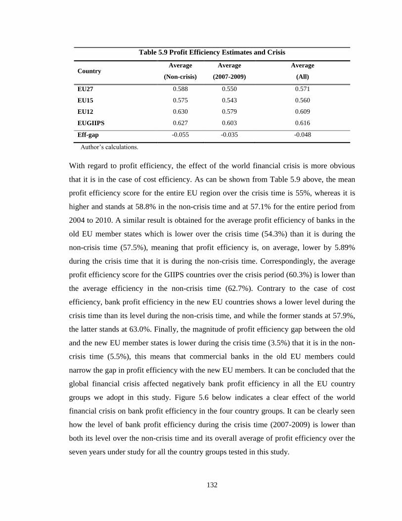
132

Table 5.9 Profit Efficiency Estimates and Crisis

Country Average

(Non-crisis)

Average

(2007-2009)

Average

(All)

EU27 0.588 0.550 0.571

EU15 0.575 0.543 0.560

EU12 0.630 0.579 0.609

EUGIIPS 0.627 0.603 0.616

Eff-gap -0.055 -0.035 -0.048


With regard to profit efficiency, the effect of the world financial crisis is more obvious

that it is in the case of cost efficiency. As can be shown from Table 5.9 above, the mean

profit efficiency score for the entire EU region over the crisis time is 55%, whereas it is

higher and stands at 58.8% in the non-crisis time and at 57.1% for the entire period from

2004 to 2010. A similar result is obtained for the average profit efficiency of banks in the

old EU member states which is lower over the crisis time (54.3%) than it is during the

non-crisis time (57.5%), meaning that profit efficiency is, on average, lower by 5.89%

during the crisis time that it is during the non-crisis time. Correspondingly, the average

profit efficiency score for the GIIPS countries over the crisis period (60.3%) is lower than

the average efficiency in the non-crisis time (62.7%). Contrary to the case of cost

efficiency, bank profit efficiency in the new EU countries shows a lower level during the

crisis time than its level during the non-crisis time, and while the former stands at 57.9%,

the latter stands at 63.0%. Finally, the magnitude of profit efficiency gap between the old

and the new EU member states is lower during the crisis time (3.5%) that it is in the non-

crisis time (5.5%), this means that commercial banks in the old EU members could

narrow the gap in profit efficiency with the new EU members. It can be concluded that the

global financial crisis affected negatively bank profit efficiency in all the EU country

groups we adopt in this study. Figure 5.6 below indicates a clear effect of the world

financial crisis on bank profit efficiency in the four country groups. It can be clearly seen

how the level of bank profit efficiency during the crisis time (2007-2009) is lower than

both its level over the non-crisis time and its overall average of profit efficiency over the

seven years under study for all the country groups tested in this study.

133

Figure 5.6. Bank Profit Efficiency and the Financial Crisis

0.48

0.50

0.52

0.54

0.56

0.58

0.60

0.62

0.64P

rofi

t E

ffic

ien

cy (

Mea

n)

Country

Profit Efficiency and Crisis

Average

(Non-crisis)

Average

(2007-2009)

Average

(All)

134


This chapter provides an empirical analysis of the levels of cost and profit efficiencies of

the European Union banking system over the period from 2004 until 2010. The results

with regard to cost and profit efficiency estimates are presented according to four

frontiers; the common frontier for the entire EU region and the separate frontiers

constructed for the old and new EU countries as well as the GIIPS countries.

Regarding cost efficiency and using the common frontier for the purpose of comparison,

we find that commercial banks in the GIIPS countries have the highest cost efficiency

average over the study time period (2004-2010), while the new EU countries experience

the lowest level of mean cost efficiency. Thus, the old EU countries’ banking systems are,

on average, more cost efficient than banking systems in the new EU countries. Based on

size groups, large banks appear to be the most cost efficient banks while the very large

banks are the least efficient. There is a positive evolution in the average cost efficiency

levels for all the four EU sub-samples and a decrease in the efficiency gap between the

old and the new EU countries over time. In addition, the results do not reveal a significant

increase in the dispersion of cost efficiency in any of the four country groups over the

period 2004-2010; however, all the EU groups experience a slight increase in efficiency

dispersion after 2007 except for the new EU members. We also find that there is a

decrease in the average cost efficiency level during the crisis time compared to its level

during the non-crisis time for all the EU country groups, with the exception of the new EU

countries.

As to profit efficiency and based on the common frontier, commercial banks in the GIIPS

countries appear to be the most profit efficient banks, on average, in the sample. Also, and

contrary to cost efficiency, the new EU member states appear to have more profit efficient

banking systems than the old EU member states. Based on size groups, very large banks

appear to be the most profit efficient banks while medium banks are the least efficient.

Additionally, there is a positive evolution in the average profit efficiency levels for all the

EU country groups and a decrease in the profit efficiency gap between the new and the

old EU countries. The dispersion of bank profit efficiency does not show significant

fluctuations over time in the case of the entire EU and the old EU countries, while it

135

experiences clear fluctuations in the case of the new EU countries and the GIIPS

countries. The world financial crisis is found to have a more obvious influence on profit

efficiency than in the case of cost efficiency. The results show that the level of profit

efficiency is lower during the crisis time than it is over the non-crisis time for all the EU

country groups.

136

Chapter 6

Risk and Determinants of Efficiency in the European Union

Banking Sector

6.1 Introduction

This chapter introduces an analysis for three types of bank risk; insolvency, liquidity and

credit risks in the EU banking system. In addition, this chapter investigates the influence

of these risk variables and other environmental variables on cost and profit inefficiencies.

We focus on the aforementioned three types of risk because, as mentioned earlier in this

thesis, we aim to investigate whether the level of these types of bank risk at the EU banks

matter during the world financial crisis in terms of banking efficiency. In other words, we

examine the role that these bank risks play during the crisis in the EU and to what extent

maintaining lower level of these risks can protect European banks in times of financial

distress with reference to banking performance. In addition, this chapter investigates the

efficiency correlates, which would provide explanations for the variations in bank

efficiency scores between banks and across countries. This investigation, as Berger and

Mester (1997) argue, might have important implications for the public policy, research

and bank management. This chapter addresses the second research question in this thesis.

Section 6.2 provides bank risk analysis concerning insolvency, credit and liquidity risks.

Section 6.3 examines and discusses the determinants of bank cost and profit

inefficiencies. And while Section 6.3.1 focuses on the effects of risk variables on bank

inefficiency, Section 6.3.2 analyses the influence of other explanatory variables. Section

6.4 investigates the rank order correlation of efficiency scores and traditional non-frontier

performance measures. Finally, Section 6.5 is the summary and conclusion.

137

6.2 Bank Risk Analysis

Before embarking on analysing the relationship between bank cost and profit efficiencies

and bank risks, we start by analysing banking risks and this includes insolvency risk;

measured by the ratio of equity to total assets, liquidity risk; measured by the ratio of total

loans to total assets, and credit risk; measured by the ratio of non-performing loans to

total gross loans. These three different bank risks are measured and analysed for the four

EU samples used in this study. Descriptive statistics; mainly the mean value of the risk

measures are used to analyse risk over the period 2004-2010 with the emphasis on the

global crisis time (2007-2009). Tables 6.1 and 6.2 display the mean values of different

bank risk measures along with the standard deviation and the number of observations for

the four groups of the EU countries.

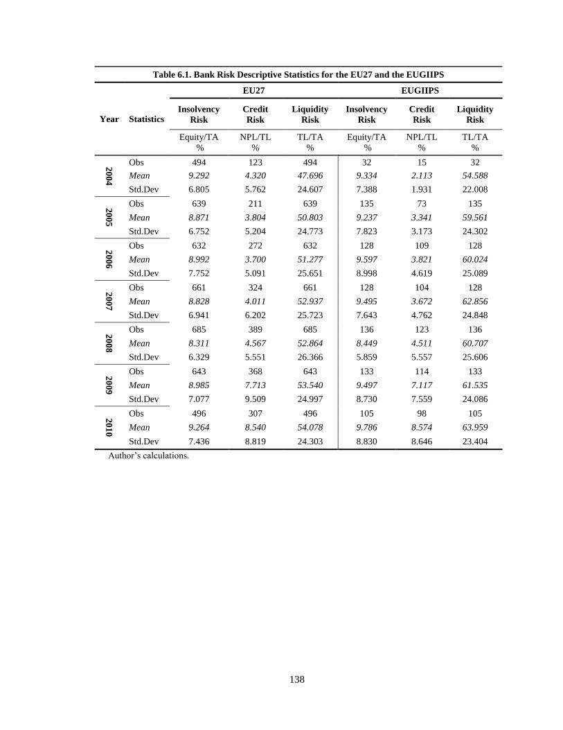
138

Table 6.1. Bank Risk Descriptive Statistics for the EU27 and the EUGIIPS

Year Statistics

EU27 EUGIIPS

Insolvency

Risk

Credit

Risk

Liquidity

Risk

Insolvency

Risk

Credit

Risk

Liquidity

Risk

Equity/TA

%

NPL/TL

%

TL/TA

%

Equity/TA

%

NPL/TL

%

TL/TA

%

20

04

Obs 494 123 494 32 15 32

Mean 9.292 4.320 47.696 9.334 2.113 54.588

Std.Dev 6.805 5.762 24.607 7.388 1.931 22.008

20

05

Obs 639 211 639 135 73 135

Mean 8.871 3.804 50.803 9.237 3.341 59.561

Std.Dev 6.752 5.204 24.773 7.823 3.173 24.302

20

06

Obs 632 272 632 128 109 128

Mean 8.992 3.700 51.277 9.597 3.821 60.024

Std.Dev 7.752 5.091 25.651 8.998 4.619 25.089

20

07

Obs 661 324 661 128 104 128

Mean 8.828 4.011 52.937 9.495 3.672 62.856

Std.Dev 6.941 6.202 25.723 7.643 4.762 24.848

20

08

Obs 685 389 685 136 123 136

Mean 8.311 4.567 52.864 8.449 4.511 60.707

Std.Dev 6.329 5.551 26.366 5.859 5.557 25.606

20

09

Obs 643 368 643 133 114 133

Mean 8.985 7.713 53.540 9.497 7.117 61.535

Std.Dev 7.077 9.509 24.997 8.730 7.559 24.086

20

10

Obs 496 307 496 105 98 105

Mean 9.264 8.540 54.078 9.786 8.574 63.959

Std.Dev 7.436 8.819 24.303 8.830 8.646 23.404


139

Table 6.2. Bank Risk Descriptive Statistics for the EU15 and the EU12

Year Statistics

EU15 EU12

Insolvency

Risk

Credit

Risk

Liquidity

Risk

Insolvency

Risk

Credit

Risk

Liquidity

Risk

Equity/TA

%

NPL/TL

%

TL/TA

%

Equity/TA

%

NPL/TL

%

TL/TA

%

20

04

Obs 373 81 373 121 42 121

Mean 8.719 3.795 47.525 11.057 5.332 48.223

Std.Dev 6.652 5.451 26.354 6.993 6.261 18.283

20

05

Obs 504 154 504 135 57 135

Mean 8.596 3.315 50.709 9.898 5.125 51.155

Std.Dev 7.020 4.193 26.377 5.541 7.147 17.612

20

06

Obs 504 203 504 128 69 128

Mean 8.871 3.329 50.322 9.466 4.792 55.039

Std.Dev 8.366 4.022 27.187 4.593 7.323 17.989

20

07

Obs 517 229 517 144 95 144

Mean 8.612 3.374 51.686 9.607 5.545 57.428

Std.Dev 7.353 4.471 27.374 5.148 8.961 17.999

20

08

Obs 538 273 538 147 116 147

Mean 7.887 3.991 50.734 9.859 5.924 60.659

Std.Dev 6.034 4.669 27.728 7.119 7.054 18.740

20

09

Obs 501 257 501 142 111 142

Mean 8.639 6.104 51.980 10.206 11.439 59.044

Std.Dev 7.175 8.219 26.547 6.604 11.153 17.519

20

10

Obs 385 216 385 111 91 111

Mean 8.940 6.744 52.919 10.390 12.804 58.097

Std.Dev 7.775 7.349 25.751 6.012 10.455 17.943



Although the equity to total assets ratio was included in the efficiency functions for the

reasons explained earlier, we include it again in this regression to examine its effect on

cost and profit inefficiencies. In this sense, we avoid including this ratio twice in our

analysis as we regress capital ratio against inefficiency here rather than efficiency

following Kasman and Yildirim (2006). Table 6.1 shows how the level of insolvency risk

changes over the study period for the entire EU region including its 27 member states and

for the five EU GIIPS countries. The equity ratio mean of the EU27 region at the

140

beginning of the period in 2004 (9.29%) is very close to its level at the end of the period

in 2010 (9.26%); however, the ratio starts to decline from 2006 onward and significantly

during the first half of the global crisis to reach 8.31% in 2008 before it starts to rise

again. The equity ratio maintained by banks in the GIIPS countries is, to some extent,

stable over the first four years before it drops considerably by more than 1% (from 9.50%

in 2007 to 8.45% in 2008) and rises to 9.79% in 2010. From Table 6.2 similar results can

be obtained for the old EU states where banks equity ratio declines significantly from

8.61% in 2007 to 7.89% in 2008; the year in which the global crisis strikes strongly the

global financial system. Finally, and contrary to the old EU countries, the mean equity

ratio of banks in the new EU states drops from 11.06% in 2004 to 9.90% in 2005,

however, it starts to rise steadily from 2006 until 2010 to reach 10.39%. The overall

standard deviation of the equity to assets ratio for the entire EU region ranges between

6.33% in 2008 and 7.75% in 2006.

Figure 6.1 below shows the time trend of the equity to total assets ratio (insolvency risk),

which shows the level of risk for the four EU groups and allows comparing the level of

insolvency risk maintained by commercial banks in the old and the new EU countries. It

can be clearly seen from the graph that banks in the new EU countries maintain, on

average, lower level of insolvency risk over time than the old EU countries, with no

evidence of an increase in this risk during the crisis time. Also, the graph shows how the

trend of capital ratio for banks in the old EU countries slightly declines between 2006 and

2007 while it sharply falls between 2007 and 2008 in parallel with the crisis event and the

losses associated with it on the assets side. The overall banking system in the entire EU

region witnesses a clear increase in insolvency risk in 2008; such increase starts from

2006 and becomes more obvious between 2007 and 2008. This analysis of equity ratio

stands in line with the discussion of Blundell-Wignall and Atkinson (2009) and Carmassi

et al. (2009) referring to the idea that banks in Europe increased their leverage before and

by the time of the global crisis, while they started deleveraging as a result of the crisis, as

the GAO (2010) argues.

141

Figure 6.1. Equity to Total Assets Ratio (Insolvency Risk)


Liquidity risk is measured by the ratio of total loans to total assets, where the mean values

of such ratio are summarised for the four samples used in Tables 6.1 and 6.2. The mean

value of total loans to total assets ratio increases significantly at the beginning of the

period in 2004 (47.70%) to reach 50.80% in 2005 and 51.28% in 2006; however, there is

no significant change during the time of the crisis in the EU27 sample. Banks in the GIIPS

countries maintain high levels of total loans to total assets ratio over the study period at

54.59% in 2004 and 63.96% in 2010. Before the crisis, the mean ratio increases from

60.02% in 2006 to 62.86% in 2007, however, during the crisis time this ratio decreases by

more than 2% (from 62.86% to 60.71%) between 2007 and 2008, while it increases again

to reach 61.56% in 2009 and 63.96% in 2010. Table 6.2 shows that, concerning the old

EU states, banks increase their liquidity risk ratio from 47.53% in 2004 to 51.69% in

2007, before it falls in 2008 (50.73%) and increases again in 2009 and 2010. Finally, the

loan to assets ratio increases dramatically from 48.22% in 2004 to 60.66% in 2008, before

7.5

8.5

9.5

10.5

11.5

2004 2005 2006 2007 2008 2009 2010

Mea

n %

Year

Equity Ratio (Solvency Risk)

EU-27

EU-15

EU-12

EU-GIIPS

142

it declines and reaches 58.10% in 2010. This means that banks in the new EU countries

maintain higher levels of liquidity risk than their counterparts in the old EU countries over

the seven years under study. The standard deviation of total loans to total assets ranges

between 24.30% in 2010 and 26.37% in 2008 for the entire EU region for the ratio.

Figure 6.2 below produces a clear image of how the mean trends of liquidity risk for the

four EU samples behave over the period 2004-2010. The figure shows that banks in the

new EU states maintain higher levels of liquidity risk than banks in the old EU states over

the seven-year period of time. Moreover, the trend of the EU27 sample goes up at the

beginning of the period before it declines in 2008 and rises up again onward. Furthermore,

banks in the four European samples increase their liquidity risk prior to the financial crisis

(before 2007) which stands in line with the discussion of Brunnermeier (2009) and

Diamond and Rejan (2009) with regard to the causes of the world crisis 2007-2009.

However, the decrease in the ratio of total loans to total assets during the crisis,

particularly in 2008 for the old EU countries, can be attributed to the difficulties of

lending and issuing loans during the economic downturn and to deleveraging and selling

off loans at banks in those countries.

Figure 6.2. Total Loans to Total Assets Ratio (Liquidity Risk)

45

50

55

60

65

2004 2005 2006 2007 2008 2009 2010

Mea

n %

Year

TL/TA (Liquidity Risk)

EU-27

EU-15

EU-12

EU-GIIPS

143


Table 6.1 shows that the mean of the non-performing loans to total loans ratio

approximately doubles between 2004 (4.32%) and 2010 (8.54%) in the banking system of

the entire EU area. The mean ratio increases significantly during the time of the crisis

where it jumps from 4.01% in 2007 to reach 7.71% in 2009, reaching 8.54% in 2010.

Regarding the GIIPS countries, the mean of credit risk increases by almost fourfold

between 2004 (2.11%) and 2010 (8.57%), experiencing large increase over the crisis time

2007-2009. Similar results in Table 6.2 can be derived for banks in the old and new EU

states where the mean of the non-performing loans ratio doubles over the period 2004 to

2010 and increases significantly during the crisis time. However, the increase in the mean

value is very large in the new EU countries over the period 2007-2010 (from 5.55% to

12.80%) compared with 3.37% in 2007 and 6.74% in 2010 for banks in the old EU

countries. The overall all standard deviation of the ratio of non-performing loans to total

loans ranges between 5.09% in 2006 and 9.51% in 2009.

Figure 6.3 below shows homogenous time trends regarding credit risk that increases from

2007 onward for all the EU groups. However, the graph reveals that the overall banking

system of the new EU states is, on average, riskier than the banking systems in the old EU

states and faces a much steeper increase in credit risk from 2008 to 2010. It is crucial here

to refer to the significant increase in the credit risk during and after the global crisis (from

2007 to 2010). That significant increase can be attributed to the tough global crisis

conditions and the economic recession it caused, which might have revealed increases in

the non-performing loans ratio and credit default between 2008 and 2010. That might also

have been exacerbated by the European sovereign debt crisis from late 2009 onward.

144

Figure 6.3. Non-Performing Loans to Total Loans Ratio (Credit Risk)

6.3 Risk and Determinants of Bank Inefficiency (Environmental

Variables)

In order to investigate possible determinants of bank cost and profit inefficiencies, bank

inefficiency is regressed on a set of bank risk variables and other independent variables.

This investigation would provide explanations for the variations in cost and profit

efficiency scores between banking systems in the European Union countries. As explained

in the methodology section, the regression is implemented through the one-step Battese

and Coelli (1995) estimation model. According to this model, bank inefficiency can be

expressed as a function of a set of environmental variables that might contribute to

different efficiency estimation scores.

For the purpose of this study, the environmental variables are divided into two main

groups, risk variables and other explanatory variables. While risk variables include

insolvency risk, liquidity risk, and credit risk, the other explanatory variables, on the other

2.0

4.0

6.0

8.0

10.0

12.0

2004 2005 2006 2007 2008 2009 2010

Mea

n %

Year

NPL/TL (Credit Risk)

EU-27

EU-15

EU-12

EU-GIIPS

145

hand, include a set of bank-specific, industry-specific, and macroeconomic variables;

among them is the world financial crisis (2007-2009). As has been done above for the

analysis of bank efficiency levels, we present the inefficiency regression analysis

according to four models. Model 1 contains the regression results based on a common

efficiency frontier (EU27), while models 2, 3, 4 provide the regression results based on

separate frontiers for the other three groups EU15, EU12, and EUGIIPS, respectively.

Tables 6.3 and 6.4 below summarise results of the regression analysis for cost inefficiency

and profit inefficiency as dependent variables, respectively. It is important to note that

separate regression is implemented when regressing inefficiency on the independent

variable the non-performing loans to gross loans ratio. This is because due to data

availability with regard to this variable we only include observations for which data on

this variable is available, meaning that observations for 528 out of total 947 EU

commercial banks are included in this regression. However, for the purpose of the

comparison between the common frontier and separate frontiers of the EU country groups,

we report results for this variable in the same column together with the other explanatory

variables. Two correlation matrices are implemented to test the strength of the correlation

between the environmental variables and we report the two matrices in Appendix 4a and

Appendix 4b. As can be seen from the two matrices tables, no high correlation numbers

are obtained between two environmental variables, meaning the problem of

multicollinearity does not exist in our regression. We first start by investigating the effects

of risk variables on bank cost and profit inefficiencies, and then we test the influence of

the other environmental variables on inefficiency.

146

Table 6.3 Determinants of Cost Inefficiency


Frontier Separate Frontier

Model 1

(EU27)

Model 2

(EU15)

Model 3

(EU12)

Model 4

(EUGIIPS)

Bank-Risk Variables

EQ λ1 0.0031***

(0.0005)

0.0029***

(0.0006)

-0.0012**

(0.0054)

0.0008

(0.0023)

EQ_CRISIS λ2 -0.0009**

(0.0005)

-0.0007**

(0.0005)

-0.0004**

(0.0058)

-0.0001

(0.0010)

TLTA λ3 -0.0263***

(0.0005)

-0.0284***

(0.0005)

-0.0214***

(0.0017)

-0.0329***

(0.0019)

TLTA_CRISIS λ4 -0.0023**

(0.0007)

-0.0003**

(0.0002)

-0.0011*

(0.0016)

-0.0013**

(0.001)

NPLTL λ5 0.0015**

(0.0013)

0.00453***

(0.0016)

0.0028*

(0.0042)

0.0037**

(0.0095)

NPLTL_CRISIS λ6 0.0037**

(0.0014)

0.0032**

(0.0026)

0.0005*

(0.0056)

-0.0012*

(0.0048)

Other Explanatory Variables

SIZE λ7 -0.0257***

(0.0074)

-0.0282***

(0.0082)

-0.0415*

(0.0381)

-0.0597*

(0.0324)

ROAA λ8 -0.0121***

(0.0014)

-0.0128***

(0.0017)

-0.0278***

(0.00686)

-0.0095*

(0.0062)

INTERMED λ9 0.0002

(0.0001)

0.00086**

(0.00002)

0.0008**

(0.0002)

-0.0002

(0.0003)

CONC λ10 -0.0005

(0.0006)

0.0005**

(0.0017)

0.0012

(0.0046)

-0.0048

(0.0035)

INFL λ11 -0.0077***

(0.0019)

-0.0128***

(0.0036)

-0.0028***

(0.0058)

-0.0137

(0.0099)

NIR λ12 -0.0021*

(0.0030)

-0.0211**

(0.0047)

0.0103*

(0.0054)

0.0517*

(0.0274)

CRISIS λ13 0.0342**

(0.0099)

0.7493*

(0.0921)

-0.1266*

(0.1150)

0.0423**

(0.0406)

C_DUMMY λ14 -0.0860*

(0.0946) ….. ….. …..

C_CRISIS λ15 0.0880*

(0.072) ….. ….. …..

GIIPS λ16 -0.1812***

(0.0652)

-0.1316**

(0.0721) ….. …..

GIIPS_CRISIS λ17 -0.0519

(0.0158)

-0.0466

(0.0164) ….. …..

Note: ***, ** and * indicate 1%, 5% and 10% significance levels, respectively, and asymptotic standard errors in

parentheses. EQ is equity ratio, EQ_CRISIS is equity and crisis interactive variable, TLTA is total loans to total assets

ratio, TLTA_CRISIS is total loans ratio and crisis interactive variable, NPLTL is non-performing loans to total loans

ratio, NPLTL_CRISIS is non-performing loans ratio and crisis interactive variable, SIZE is bank size, ROAA is return

on average assets, INTERMED is intermediation ratio, CONC is market concentration, INFL is inflation, NIR is nominal

interest rate, CRISIS is the world financial crisis 2007-2009, C_DUMMY is old countries dummy variable, C_CRISIS is

old countries and crisis interactive variable, GIIPS is GIIPS countries dummy variable, and GIIPS_CRISIS is GIIPS and

crisis interactive variable.

147

Table 6.4 Determinants of Profit Inefficiency


Frontier Separate Frontier

Model 1

(EU27)

Model 2

(EU15)

Model 3

(EU12)

Model 4

(EUGIIPS)

Bank-Risk Variables

EQ λ1 0.0096***

(0.0009)

0.0114***

(0.0011)

0.0192***

(0.0054)

0.0141**

(0.0055)

EQ_CRISIS λ2 -0.0029***

(0.0009)

-0.0021**

(0.0011)

-0.0159***

(0.0075)

-0.0135**

(0.0051)

TLTA λ3 -0.0072***

(0.0006)

-0.0090***

(0.0006)

-0.0138***

(0.0053)

-0.0128***

(0.0031)

TLTA_CRISIS λ4 0.0013***

(0.0004)

0.0014***

(0.0004)

0.0014***

(0.0015)

0.0034*

(0.0024)

NPLTL λ5 0.0117***

(0.0117)

0.0144***

(0.0031)

0.0047**

(0.0027)

0.0181**

(0.0022)

NPLTL_CRISIS λ6 0.0066*

(0.0024)

0.0042*

(0.0031)

0.0029

(0.0041)

0.0022

(0.0065)


SIZE λ7 -0.0740***

(0.0116)

-0.0745**

(0.0143)

-0.1099**

(0.0375)

0.0123

(0.0719)

ROAA λ8 -0.0158***

(0.0013)

-0.0152***

(0.0018)

-0.0246***

(0.0031)

-0.0575***

(0.0094)

INTERMED λ9 -0.0001**

(0.00007)

0.0003*

(0.00003)

-0.0013**

(0.0003)

0.0005

(0.0005)

CONC λ10 -0.0024**

(0.0009)

-0.0019**

(0.0011)

-0.0076**

(0.0033)

-0.0087

(0.0055)

INFL λ11 0.0097***

(0.0039)

0.0167***

(0.0063)

0.0099***

(0.0054)

0.0042***

(0.0192)

NIR λ12 0.0220***

(0.0036)

0.0664**

(0.0117)

0.0139***

(0.0043)

0.0774

(0.0471)

CRISIS λ13 0.3057**

(0.1369)

0.0507**

(0.0256)

0.0239**

(0.0926)

0.1495**

(0.1257)

C_DUMMY λ14 0.2824***

(0.0987) ….. ….. …..

C_CRISIS λ15 0.0468

(0.0361) ….. ….. …..

GIIPS λ16 -0.0865

(0.0880)

-0.0995*

(0.0027) ….. …..

GIIPS_CRISIS λ17 -0.0221

(0.0334)

-0.0132

(0.0351) ….. …..


parentheses. EQ is equity ratio, EQ_CRISIS is equity and crisis interactive variable, TLTA is total loans to total assets

ratio, TLTA_CRISIS is total loans ratio and crisis interactive variable, NPLTL is non-performing loans to total loans

ratio, NPLTL_CRISIS is non-performing loans ratio and crisis interactive variable, SIZE is bank size, ROAA is return on

average assets, INTERMED is intermediation ratio, CONC is market concentration, INFL is inflation, NIR is nominal

interest rate, CRISIS is the world financial crisis 2007-2009, C_DUMMY is old countries dummy variable, C_CRISIS is

old countries and crisis interactive variable, GIIPS is GIIPS countries dummy variable, and GIIPS_CRISIS is GIIPS and

crisis interactive variable.

148

6.3.1 Bank Risk Effects on Inefficiency

We use equity to assets ratio, total loans to total assets ratio, and non-performing loans to

total gross loans ratio to measure the effects of insolvency risk, liquidity risk, and credit

risk on bank cost and profit inefficiencies. Moreover, we investigate the effect of these

risks on inefficiency during the crisis time by interacting the aforementioned variables

with the world financial crisis dummy variable, as explained earlier in this study. The

purpose of investigating the effects of such interactive variables on bank inefficiency is to

find out whether commercial banks with lower levels of risk better withstand the world

financial crisis in the EU; Or to put it another way, we examine to what extent the level of

risk affects the performance of EU banks during the crisis period. We start with

insolvency risk, and then we move to liquidity risk and credit risk thereafter.


The first risk variable to be investigated with regard to its effect on bank inefficiency is

the capital ratio that represents insolvency risk. With regard to cost inefficiency, Table 6.3

shows that the coefficient of equity ratio has a negative sign in Model 3 (the new EU

states) only, while it appears to be positive in the other three models. According to the

common frontier of the entire EU region (Model 1), equity ratio has a positive and highly

significant effect on cost inefficiency, meaning that less capitalised commercial banks are

more cost efficient than well capitalised banks over the seven years under study. Similar

results are shown for the separate frontier of the old EU states (Model 2) where the effect

of this variable is positive and highly significant on cost inefficiency. The inverse

relationship between bank cost efficiency and equity capital might be attributed to the idea

that debt financing is cheaper than raising equity capital, hence more leveraged

commercial banks appear to be more cost efficient than more capitalised banks. This

reverse relationship between equity ratio and bank efficiency stands in line with the

results obtained by Altunbas et al. (2007), by Allen and Rai (1996) and by Sun and

Change (2011). On the other hand, equity ratio positively affects bank efficiency in the

new EU states (EU12), meaning that well-capitalised banks in the new EU countries are

more cost efficient than their counterparts with less equity capital. It can be said that as

capital is more expensive than debt, this imposes pressure on banks in the new EU

149

countries to reduce their operating costs. This stands in line with the result obtained by

Fries and Taci (2005) and Yildirim and Philippatos (2007).

Regarding profit inefficiency, equity ratio has a positive and significant influence on

profit inefficiency in all models, meaning that well-capitalised commercial banks are

more profit inefficient that their counterparts in the European Union. This is because

equity capital is more expensive than debts, which therefore increase bank costs

associated with issuing equities and decrease bank profits. Also, this result complies with

the moral hazard hypothesis that a bank with solvency problems would undertake risky

business and invest in profitable activities, which therefore lead the bank to appear

efficient in the short-term while paying for the consequence of its risky assets in the long-

term. Similar results are obtained by Hasan and Marton (2003) who find positive impact

of equity ratio on profit inefficiency in the Hungarian banking system.

Equity Ratio * Crisis

Concerning the effect of equity ratio on cost inefficiency during the crisis time, Table 6.3

shows how, overall, the sign of equity ratio coefficient shifts from positive to negative

over the crisis time in all models, meaning that the interactive variable of equity ratio and

the crisis dummy negatively affect cost inefficiency. This supports our hypothesis that

commercial banks in the EU with higher level of capital (lower insolvency risk) appear

more cost efficient and less affected by the crisis than banks with higher leverage ratio.

That is because such banks might have been able to borrow at cheaper prices as they are

considered safer and sounder in such severe downturn and credit crunch time. The

coefficient of this interactive variable is negative and significant (at 5 %) in all models

except for Model 4 (the GIIPS countries) where it is insignificant.

Concerning bank profit inefficiency, the results are similar to those in the case of cost

inefficiency, as can be seen from Table 6.4. The coefficient sign of equity ratio becomes

negative and significant after interacting it with the world crisis dummy in all the four

models, meaning that the capital ratio negatively and significantly affects profit

inefficiency in the EU banking system during the crisis time. Again, this stands in line

with our expectations as banks with higher capital might have faced lower costs with

150

regard to borrowing compared to those with lower capital (riskier). So it can be concluded

here that commercial banks with higher levels of capital (lower level of leverage)

outperform their counterparts in terms of cost and profit efficiencies during the crisis time.

In other words, well-capitalised commercial banks (with less insolvency risk) were able to

better withstand the world financial crisis than less capitalised banks in the European

Union.


The second risk variable whose effect on bank efficiency is to be examined in this study is

the ratio of total net loans to total assets as a proxy liquidity risk. Table 6.3 reveals a

negative and highly significant relationship between the ratio of total loans to total assets

and bank cost inefficiency, meaning that lower liquidity position (larger amount of loans)

is positively connected with cost efficiency, which is not our expected sign. This inverse

association between cost inefficiency and the amount of loans holds for the four models,

meaning that more aggressive commercial banks (engaged in more lending activities) in

the EU are more cost efficient. In other words, commercial banks that operate more

efficiently in terms of costs are more successful and have better capability to expand their

loans business in the EU market. Although we expected a reverse relationship between

this variable and cost inefficiency, a similar result is obtained by Altunbas et al. (2007),

Yildirim and Philippatos (2007), Allen and Rai (1996), and Maudos et al. (2002a).

With regard to profit inefficiency, as we expected, a negative and highly significant

relationship between the ratio of loans to total assets and profit inefficiency is confirmed

in all the four models. This means that commercial banks with higher liquidity risk

(higher level of loans) operate more profit efficiently than banks with lower loans to

assets ratio in the EU market. This stands in line with the idea that higher profits are

consistent with more risky position, or with the conventional concept of the trade-off

between liquidity and profitability, as higher liquidity level leads to lower profitability due

to the opportunity costs accompanied with maintaining a high level of liquidity.

Moreover, it might be attributed to the idea that, as Berger and Mester (1997: 39) argue,

“banks’ loan products are more highly valued than securities, or it could reflect higher

151

market power that exists in loan markets compared to the other product markets in which

banks operate.”

Total Loans/Total Assets * Crisis

As to cost inefficiency, Table 6.3 again reveals a negative relationship between the ratio

of total net loans to total assets multiplied by the crisis dummy and bank cost inefficiency

in all the four models, which is again not our expected sign. These results mean that banks

with higher loans to assets ratio are more cost efficient than their counterparts during the

crisis time (2007-2009) as they are in the non-crisis time. Put it differently, commercial

banks that operate more cost efficiently during the crisis period are more successful to

expand their loan business in the EU markets.

On the other hand, the effect of the world crisis on the relationship between liquidity risk

and bank profit inefficiency is obvious as the sign of this relationship reverses into

positive when the interactive variable of liquidity and crisis dummy is created. This

relationship is positive and highly significant in all models except in Model 4. This

outcome suggests that commercial banks with higher loans to assets ratios appear to be

less profit efficient during the crisis time, meaning that banks with more liquidity (less

loans) over the financial crisis outperform their counterparts in reference to profit

efficiency. That might be attributed to the loss associated with loan defaults over the crisis

time and as Figure 6.3 in section 6.2 earlier shows, there is an increase in the percentage

of non-performing loans during the period 2007-2009 which might have increased losses

and decrease profitability as a consequence. Also, it might be attributed to the ability of

more liquid banks to meet deposit withdrawals and other obligations without facing

additional costs. Therefore, it can be concluded here that commercial banks with smaller

amount of loans relative to total assets (more liquid banks) outperform their counterparts

in terms of profit efficiency during the crisis time, though these banks fail to outperform

less liquid banks in terms of cost efficiency. In other words, banks with less liquidity risk

could withstand better the world crisis than less liquid banks in reference to profit

maximisation but not in reference to costs minimisation.

152


The third risk variable to be investigated in this study is credit risk that is represented here

by the ratio of non-performing loans to total loans. As can be seen from Table 6.3, there is

a positive and significant effect of the ratio of non-performing loans (bad loans) to total

loans on cost inefficiency in all four models. This suggests that commercial banks with

higher amounts of bad loans are the least cost efficient banks in the EU, particularly in the

old EU member states. This result is consistent with our expectations that the increase in

the amount of non-performing loans would raise expenses related to handling such loans

which in turn decreases bank cost efficiency. Therefore, it can be concluded from our

result that commercial banks with higher cost efficiency are better at evaluating credit

risk. This complies with the results obtained by Berger and De Young (1997), Fries and

Taci (2005), and Altunbas et al. (2000).

Regarding bank profit inefficiency, Table 6.4 shows that this variable has a positive and

significant influence on bank profit inefficiency, meaning that commercial banks with

smaller amounts of bad loans are more profit efficient. These results stand in line with our

expectations that non-performing loans increase the expenses associated with handling

them and with the loan loss provision put aside to face the expected default of such loans,

which in turn decrease bank profits.

Non-Performing Loans/Gross Loans * Crisis

By the time of the world financial crisis, there was an increase in the credit risk held at the

financial institutions in the US and the EU due to different factors. From Table 6.3, it can

be shown that the interactive variable of credit risk and crisis dummy has a positive and

significant (at 5%) effect on cost inefficiency in Model 1 (EU27). This stands in line with

our expectations that higher amounts of non-performing loans during the crisis time

would increase costs related to handling such bad loans, such as the expense related to

screening, working out or selling off such bad loans. This means, again, that commercial

banks maintaining less bad loans during the crisis time appear to be more cost efficient

than their counterparts. However, in Model 4, in which a separate frontier is constructed

for the GIIPS countries, the effect of this interactive variable on bank cost inefficiency is

negative and significant (at 10%), which does not comply with our expectations. This

means that banks with more bad loans in the GIIPS countries are more cost efficient than

153

banks with less bad loans over the crisis time. This can be interpreted by the “cost

skimping” hypothesis suggested by Berger and De Young (1997) which refers to a trade-

off between short-term cost efficiency and future risk taking. Under this hypothesis, a

bank appears to be more cost efficient as it devotes fewer resources to “screening loan

customers, appraising collateral, and monitoring and controlling borrowers after loans are

issued [which] makes the bank appear to be cost efficient in the short run” (p.853). Thus,

the stock of non-performing loans remains unaffected in the short run, while this stock

increases in the future, leading to increases in the expenses associated with dealing with

these bad loans.

As to profit inefficiency, Table 6.4 shows that this interactive variable has the expected

positive effect on profit inefficiency in all models; though the effect is significant only at

10% in Model 1. This means that a higher amount of non-performing loans has a positive

but weak effect on profit inefficiency in the EU overall and in the old EU countries and a

non-significant effect in the new and in the GIIPS EU countries during the crisis period.

Consequently, it can be concluded here, in comparison with the studies that highlight the

role of credit risk in the financial crisis, that commercial banks with lower amounts of

non-performing loans (lower credit risk) outperform their peers in terms of cost

efficiency, with the exception of banks in the GIIPS countries, and in terms of profit

efficiency, particularly in the old EU states, during the financial crisis period.

6.3.2 Other Variables’ Effects on Inefficiency

Size

Further to the above discussion, we investigate whether bank-specific, industry-specific

and macroeconomic variables can explain efficiency differences between countries and

among banks. The first variable which belongs to the bank-specific category is bank size,

measured as the logarithm of bank total assets. Concerning cost inefficiency, Table 6.3

above shows that banks size is negatively associated with bank cost inefficiency in all the

four models, and it is highly significant (at 1%) in Model 1 and Model 2, while it is

significant at 10 % in Model 3 and Model 4. This stands in line with our expectations that

larger banks might have benefited from economies of scale and scope from growth and

154

joint production, which increase efficiency. Also, larger banks might benefit from a better

and more professional management team which is more able to control costs and increase

revenues. This outcome is similar to that obtained by Hasan and Marton (2003), Yildirim

and Philippatos (2007) and Matousek and Taci (2004).

Regarding profit inefficiency, it can be seen from Table 6.4 that there is a negative and

significant effect of bank size on bank profit inefficiency in all models except in the case

of Model 4 (EUGIIPS). For the groups of the entire EU region, the old EU countries, and

the new EU countries larger commercial banks appear to operate more profit efficiently

than smaller banks, again, probably due to the lower costs resulting probably from

exploiting economies of scale and economies of scope, which complies with our

expectations and results obtained by Yildirim and Philippatos (2007). Furthermore, it can

be explained through the concept of too-big-to-fail, where larger banks invest in highly

risky assets leading to higher profitability. On the other hand, in the GIIPS countries

(Model 4), the size variable appears to have a positive influence on bank profit

inefficiency, meaning that smaller banks are more efficient. This might be due to the fact

that smaller banks in the GIIPS countries issue more risky loans or deal with small size

customers in return for higher interest rates, the coefficient of this variable is insignificant

though.

Return on Average Assets (ROAA)

The second bank-specific variable to be investigated in the other explanatory variables

category is the return on average assets. With regard to cost inefficiency, it can be

concluded from Table 6.3 that the return on average assets has a negative effect on cost

inefficiency in all the four models and this effect is highly significant at 1% in Models 1,

2 and 3, while it is significant at 10% in Model 4. This means that commercial banks with

higher return on average assets appear to be more cost efficient than their counterparts

with lower return on average assets ratio. This result is identical to the results obtained by

Carbo et al. (2002) and Lensik et al. (2008).

As to profit inefficiency, Table 6.4 indicates a negative and highly significant effect of

this variable on profit inefficiency for all the EU country groups (all models). This means

155

that commercial banks with higher return on average assets ratios operate more efficiently

in terms of profit than banks with lower return on average assets ratios. This stands in line

with the belief that better utilisation of bank assets enhances bank profit efficiency, and

this result resembles the result obtained by Chan and Abd Karim (2010). If the return on

average assets can be seen as a performance measure, then it is not surprising that it is

positively correlated with both cost and profit efficiencies.

Intermediation Ratio

The third bank-specific variable to be investigated in this study is the intermediation ratio

calculated by dividing total loans by total deposits. Table 6.3 shows that the expected

negative effect of this variable on cost inefficiency is confirmed only in the GIIPS

countries (Model 4) even though it is not significant. However, the intermediation

variable is found to have a positive effect on cost inefficiency in Models 1, 2 and 3 while

it is only significant in Model 1 and Model 2. Therefore, it can be concluded that banks

with lower intermediation ratios operate more efficiently in terms of costs than their

counterparts in the entire EU and new and old EU countries, while the reverse is true in

the case of GIIPS countries. The positive relationship between cost inefficiency and the

intermediation ratio might be attributed to the higher costs associated with converting

deposits into loans, such as screening and creditworthiness evaluation costs, than

converting deposits into other investments that might be associated with lower costs.

With regard to profit inefficiency, Table 6.4 also shows mixed results as this variable

appears to have a negative and significant effect on profit inefficiency only in Model 1

(EU27) and Model 3 (EU12), while in Models 2 and 4 the effect is positive and significant

at 10% only in Model 2. This means that banks with higher intermediation ratios are more

profit efficient than their counterparts under the common frontier of the entire EU region

and in the new EU countries, while this is not confirmed under the old EU states and the

GIIPS countries separate frontiers.

Market Concentration

An industry-specific variable whose effect on cost and profit inefficiencies is examined in

this study is market concentration calculated as the sum of total assets of the five largest

156

banks divided by the total assets of the entire banking system. Regarding cost

inefficiency, the only significant (at 5%) influence this variable has is on cost inefficiency

in Model 2 (EU15) and it is positive. This means that commercial banks in the old EU

countries feel less pressure to control their costs in a concentrated environment so that

they might spend more money on their stuff and other personnel expenses, which, in turn,

might support the idea that concentration is a result of market power in these countries.

In terms of profit inefficiency, as we expected, the effect of market concentration on profit

inefficiency is negative in all models while it is only significant in Models 1, 2, and 3 at

5% but not in Model 4, as can be seen from Table 6.4. This result suggests that

commercial banks in more concentrated market (less competitive environment) have

greater market power and hence they have better ability to increase their profits in the EU

and therefore appear to be more profit efficient. In other words, commercial banks are

proved to be more profit efficient when operating in less competitive market in the EU as

a whole, in the old EU countries, and in the new EU countries on average but this result is

not strong enough to be confirmed in the EU GIIPS countries.

Inflation Rate

The first macroeconomic variable to be investigated with regard to its possible effect on

bank cost and profit inefficiencies is inflation rate. Table 6.3 shows a negative influence

by inflation rate on bank cost inefficiency in all four models, while the coefficient of this

variable appears to be insignificant in Model 4 (EUGIIPS). This suggests that commercial

banks operate more cost efficiently in an inflationary environment than in a deflationary

environment in the EU region overall, while this result is less obvious in the GIIPS

countries within the EU. This can be attributed to the belief that commercial banks in the

EU have fairly good capability with regard to forecasting the changes in the inflation rate

so as to take preparatory procedures to decrease costs associated with more inflationary

markets.

On the other hand, Table 6.4 reveals entirely different outcomes concerning how inflation

affects profit inefficiency. It can be seen from the table that the effect of inflation rate on

bank profit efficiency is negative and highly significant (at 1%) in all four models,

157

meaning that higher inflation increases profit inefficiencies of commercial banks in the

EU area. This contradicts with what is concluded in the case of cost inefficiency as banks

are said to be successful in forecasting the future inflation rate and handling their costs

based on their successful forecasting. However, it can be argued here that even if

commercial banks are successful in forecasting the future inflation rate, they might be

more flexible in terms of decreasing the costs associated with inflationary environment

than in terms of increasing their profit in the same environment. Also, it can be explained

that banks fail to impose enough increase on their lending interest rate, probably to remain

competitive, so as to offset a specific increase in inflation rate, and therefore decrease

their profits. Furthermore, inflation overall plays the main role in decreasing the value of

money, and thus higher inflation might decrease the value of money used by banks in

different investments, leading to lower profitability.

Nominal Interest Rate

The nominal interest rate is calculated as the long-term government bond yield. As can be

seen from Table 6.3, the result is mixed with regard to the influence of nominal interest

rate on bank cost inefficiency. While the effect is negative for the entire EU region

(Model 1) and the old EU countries (Model 2), it is positive for the new EU countries and

the GIIPS countries, and it is not highly significant in all four models. This indicates that

our expected positive sign holds only in the case of the new EU states and the GIIPS

countries where banks face increases in their costs with the rise in interest rate. In

contrast, higher interest rate increases cost efficiency in the main model (entire EU) and

the old EU member states possibly due to the better hedging strategy against interest rate

movements followed by commercial banks in the old member states.

As to profit inefficiency, Table 6.4 reveals positive influence by interest rate on profit

inefficiency in all models; this influence is insignificant in Model 4 (EUGIIPS) though.

This suggests that commercial banks face contractions in their profits generated as the

nominal interest rate rises according to all common and separate frontiers adopted in this

study. This might be attributed to the belief that commercial banks in the EU have an

excess of flexible-rate liabilities over flexible-rate assets or to the weak hedging strategies

run by those banks with regard to generating profits.

158

World Financial Crisis (2007-2009)

The US subprime crisis spilled over to the EU and became a world financial crisis as a

result of the financial contagion through financial sector and trade linkages between the

two regions. Starting with cost inefficiency, Table 6.3 shows that for the main model

(Model 1) the variable of the crisis affects positively and significantly (at 5%) bank cost

inefficiency, meaning that during the crisis time commercial banks face deterioration in

their cost efficiency (increase in total costs) in the entire EU region, on average. A similar

result is revealed in Model 2 (EU15) and Model 4 (EUGIIPS) where the effect of the

crisis is also positive and significant, meaning that banks’ cost efficiency decreases over

the crisis time in the old EU members and the GIIPS countries, respectively. These results

are not surprising as banks might encounter higher costs related to more expensive

borrowing in a low liquid environment, to higher costs associated with raising capital

(deleveraging), and to more expenses devoted to monitoring and evaluating

creditworthiness of clients (expenses related to risk management). However, our expected

sign does not hold in the case of the new EU member states (Model 3) where the crisis

variable has a negative influence on cost inefficiency, meaning that banks in these

countries manage to decrease their total costs over the crisis time. In other words,

commercial banks in the new EU countries appear to be more efficient in terms of cost

during the crisis years than in other years, the coefficient of this variable is only

significant at 10% though.

With regard to profit inefficiency, the coefficient of the world financial crisis is positive in

all the four models and significant at 5%. This means that the level of profit efficiency of

commercial banks in the EU deteriorates over the crisis time, or in other words, banks in

the EU appear to be more profit efficient in the non-crisis time over the period under

study. This stands in line with our expectations that banks’ profits decrease over the crisis

period probably due to weaker investing and lending business associated with lower

liquidity caused by deposits withdrawals and more difficult borrowing by banks.

Moreover, losses associated with loan defaults and other assets and the increase in total

costs at banks over the crisis time might also contribute to the deterioration in profit

efficiency.

159

Country Dummy

For the purpose of making a comparison between the efficiency levels of banking systems

in the old and the new EU member states, we include in the regression a dummy variable

for the old EU countries. This variable is only included in the main model (Model 1)

where we pool all banks from all the 27 EU countries together and run the regression

under a common frontier. As Table 6.3 shows, the effect of this variable on cost

inefficiency is negative and significant at 10% which means that commercial banks in the

old EU member states are, overall, more cost efficient than their counterparts in the new

EU countries. This stands in line with our expectations that banks in the old EU countries

operate in a more competitive environment that imposes pressure on them to reduce their

costs in addition to better technology and management techniques that help them appear

more cost efficient.

In contrast, Table 6.4 reveals a positive and highly significant effect of this variable on

bank profit inefficiency meaning that banks operating in the new EU countries are more

profit efficient than banks in the old EU countries. This, as explained earlier in this study,

might be attributed to the belief that commercial banks probably operate in a less

competitive environment in the new EU members, allowing them to make higher profits

compared to banks in the old EU members where the level of competition in the market is

much higher. These results with regard to the effect of country dummy variable on cost

and profit inefficiencies support what we concluded in the bank efficiency analysis

section earlier above, that a bank efficiency gap exists between the old and new EU

countries. While this gap is in favour of the old EU countries in the case of cost

efficiency, it is in favour of the new EU countries in the case of profit efficiency.


As we use a large sample that consists of commercial banks operating in 27 EU member

states, it is unlikely that the world crisis hit banking systems equally in those countries.

For this reason we investigate, using this interactive variable, whether banking systems in

the old and new EU countries, on average, react equally or differently to the world crisis

in terms of efficiency. Table 6.3 indicates that, as expected, this variable has a positive

160

and significant (at 10%) influence on bank cost inefficiency, meaning that the negative

effect of the world crisis on cost efficiency is stronger in the case of the old EU countries

compared to that in the case of new EU countries. This might be attributed to the idea that

the old EU countries are more integrated with the US banking and financial system as

well as the belief that financial institutions in those countries invested more in the US

mortgage toxic securities and other related securities than those in the new EU countries.

Therefore, financial contagion (through financial sector and trade linkages) played an

important role for the stronger spread of the US crisis to the old EU member states than to

the new EU states. For instance, Shirai (2009) argues that by the end of 2007, the UK,

France and Germany were among the top five countries in which the United States had its

largest cross-border stock investments, and the UK was the most active foreign investor in

the US stocks. Moreover, UK, France and Germany were among the top five countries in

which the United States held substantial amount of debt securities, while the UK was the

third largest foreign investor in US debt securities. On the other hand, and as can be seen

from Table 6.4, this interactive variable has no significant effect on profit inefficiency,

meaning that there is no solid evidence that the crisis affects differently banking profit

efficiency in the two groups.

GIIPS-Dummy

We use this variable to investigate whether commercial banks operating in the GIIPS

countries differ from other EU banks operating in the other EU member states in terms of

their efficiency level. Unfortunately, as stated above, the Eurozone crisis that has its roots

mainly in the GIIPS countries is still on-going after 2010 while we only have data till

2010. For this reason we have no specific expectations with regard to the effect of this

variable on bank cost and profit inefficiencies. We include this variable in the main model

(Model 1) and in Model 2.

As can be noticed from Table 6.3, the effect of the GIIPS dummy variable on cost

inefficiency is negative and highly significant (at 1%) in the main model (Model 1),

meaning that commercial banks in the GIIPS countries are more cost efficient than banks

in the other 22 EU countries over the period under study. Similarly, in Model 2 the effect

of this variable is negative and significant at 5%, suggesting that banks in the GIIPS

161

countries are less cost inefficient than their counterparts in the other old EU member

states. With regard to profit inefficiency, Table 6.4 shows that, again, this variable has a

negative influence on profit inefficiency according to Model 1 and Model 2; however this

influence is insignificant in the main model and only significant at 10% in Model 2. This

suggests that there is no evidence that banks in the GIIPS countries operate more

efficiently, overall, in terms of profit than banks in the other EU member states, whereas

there is some evidence that banks in the GIIPS states outperform their peers in the old EU

countries with regard to profit efficiency.

GIIPS -Dummy * Crisis

We include this variable to find out whether the world financial crisis affects bank

efficiency differently in the GIIPS countries and in the other EU member states, and we

include this variable in Model 1 and Model 2. As can be seen from Table 6.3, the effect of

this interactive variable on cost inefficiency is negative but insignificant in Model 1 and

Model 2. With regard to profit inefficiency, this variable appears also to have a negative

but insignificant effect on profit inefficiency in the two models, meaning that there is no

solid evidence that banks in the GIIPS countries operate more cost or profit efficiently

during the world crisis time than the other banks in the other EU member states.

6.4 Rank Order Correlation of Efficiency Scores and Traditional Non-

Frontier Performance Measures

Bauer et al. (1998) argue that identifying the rough ordering of which banks are more

efficient based on parametric and non-parametric approaches is more important than

generating the efficiency scores because that would help the regulators decide whether a

particular regulatory decision would be useful and effective in improving the efficiency of

banks. In our study we only use the parametric approach; the stochastic frontier approach

(SFA), to estimate bank cost and profit efficiencies of European Union commercial banks.

For this reason, we adopt the Spearman rank order correlation technique to see whether

similar rankings of banks can be obtained based on cost and profit efficiency scores

162

generated using the stochastic frontier approach, and this technique is considered as an

indicator of consistency by Bauer et al. (1998). Furthermore, we use the same technique

to find out if the SFA (in terms of both cost and profit efficiencies) and standard financial

ratios (non-frontier measures) can generate similar rankings of banks in our study. If

similar results with regard to bank rankings can be generated from the two methods, then

that would increase the confidence of the policy makers that the estimated efficiencies are

accurate indicators of performance (Bauer et al., 1998).

The two frontier efficiency measures are the cost and profit efficiencies generated using

the stochastic frontier approach, while four standard financial ratios that are popular

measures of bank performance are used for the application of Spearman rank order

correlation. These financial ratios are the return on average assets (ROAA); the total costs

to total assets ratio (TC/TA); the equity to total assets ratio (EQ/TA); and the total loans to

total deposits ratio (LOAN/DEPOSIT). The first ratio, return on average assets, is used to

assess bank profitability with higher values mean more efficient use of bank assets. The

second ratio, total costs to total assets ratio, is used as an indicator of economic

optimisation with reference to banks’ costs since it measures banks’ costs relative to bank

size. The third ratio, equity to total assets, is a measure of insolvency of financial risk with

higher ratio implies less risky bank, as explained earlier in this study. Finally, the loans to

deposits ratio, representing the intermediation ratio with higher values, refers to the higher

ability of a bank to convert its deposits into loans.

Table 6.5 below summarises the pairwise Spearman rank order correlation coefficients

between bank cost and profit efficiency scores, and between them and the standard

financial ratios aforementioned. It can be seen from the table that the Spearman rank order

correlation between cost and profit efficiencies are positive and significant at 1%,

however, the correlation is fairly low and stands at 0.24. This means that the rankings of

banks given by cost and profit efficiencies are somewhat consistent, suggesting that the

most cost efficient banks are also the most profit efficient banks. Table 6.5 also shows that

the rank correlation of the return on average assets and both cost and profit efficiency is

positive and significant, suggesting that the most cost and profit efficient banks have the

highest return on average assets ratio, the correlation is very low though. Moreover, and

163

not surprisingly, total costs to total assets ratio appears to have a negative and highly

significant rank order correlation with both cost and profit efficiencies, meaning that the

most cost and profit efficient banks have the lowest costs to assets ratios. While the rank

order correlation between costs to assets ratio and cost efficiency stands at (0.66), it is

slightly lower between this ratio and profit efficiency (0.53). We also observe a positive

and rank order correlation between equity ratio and cost and profit efficiencies, and this

correlation is significant at 1% in the case of cost efficiency and at 5% in the case of profit

efficiency. This might suggest that the most cost and profit efficient banks maintain the

highest level of equity capital. Finally, we observe a negative and significant (at 5%) rank

order correlation between the loans to deposits ratio and cost efficiency, suggesting that

there is some evidence that the most cost efficient banks have the lowest intermediation

ratio, and this correlation is fairly high at 0.56. On the other hand, this ratio has a positive

and significant (at 10%) rank order correlation with profit efficiency, indicating that there

is some weak evidence that the most profit efficient banks have the highest loans to

deposits ratios and the correlation is fairly low at 0.33.

Table 6.5 Spearman's Rank Order Correlation of Efficiency and Traditional Performance Measures

Costeff

Profiteff

Costeff

1.0000

Profiteff

0.2424***

1.0000

ROAA

0.0315**

0.0859***

TC/TA

-0.6577***

-0.5268***

EQ/TA

0.1052***

0.1091**

LOAN/DEPOSIT

-0.5592**

0.3340*

Notes: Costeff = cost efficiency; Profiteff = profit efficiency; ROAA = return on average assets; TC/TA = total costs/

total assets; EQ/TA = equity/total assets. ***, ** and * indicate that correlation is significant at 1%, 5% and 10%,

respectively.

164


This chapter presents a descriptive analysis for bank risks and investigates the

determinants of cost and profit inefficiencies. The analysis shows that, overall, the new

EU countries maintain the lowest level of insolvency risk (highest level of capital ratio),

while the old EU countries have the highest level of insolvency risk over the seven years

under study. Also, there is a clear increase in this risk before and during the world

financial crisis period for all the EU groups except for the new EU members. However, in

terms of credit risk, the new EU states appear to be the riskiest among the other country

groups with the old EU countries being the least risky, and there is increase in this risk for

all the groups by the crisis time. Concerning bank liquidity risk, the results conclude that

the old EU countries are the least risky in the sample over time, with a clear increase in

this risk for the new EU countries before the crisis time.

The determinants of cost and profit inefficiencies are investigated in the regression of the

Battese and Coelli (1995) one-step model in this chapter and are divided into risk

variables and other explanatory variables. We investigate the effects of the three risk

variables aforementioned in addition to their effects on bank inefficiency during the crisis

time. The results show that the capital ratio has, in general, a positive effect on both cost

and profit inefficiencies, while this effect shifts to negative during the crisis, suggesting

that better capitalised banks (with less insolvency risk) perform better over the crisis than

less capitalised banks in terms of both cost and profit efficiencies. Loans to assets ratio

(liquidity risk) affects negatively both cost and profit inefficiencies, while this effect turns

to positive during the crisis time only in the case of profit inefficiency. This means that

more liquid banks outperform their counterparts in terms of profit maximisation during

the crisis. Furthermore, the ratio of non-performing loans to gross loans (credit risk) has a

positive effect on cost and profit inefficiencies over the crisis and non-crisis time and this

effect is more significant in the case of cost inefficiency than profit inefficiency over the

crisis. This suggests that banks with lower credit risk appear to be more cost and profit

efficient over stable and non-stable economic conditions. Therefore, it can be concluded

here that the level of these bank risks matters during the crisis time and banks that

maintain higher level of such risks appear less efficient over the financial crisis time in the

165

EU. The regression results, also, show that the financial crisis has a positive influence on

cost and profit inefficiencies, meaning that commercial banks in the EU perform better in

the non-crisis time. Finally, this chapter examines the Spearman rank order correlation of

efficiency scores and conventional accounting based performance measures. We find that

cost and profit efficiencies are significantly and positively correlated with each other

meaning that most cost efficient banks are also most profit efficient banks, but the

correlation is fairly low. Return on average assets, cost to assets ratio, equity to assets

ratio and loans to deposits ratio are also, in general, significantly correlated with both cost

and profit efficiencies.

166

Chapter 7

Bank Stock Performance, Efficiency and Risk in the EU

Markets

7.1 Introduction

Over the past two decades, competitive pressures have progressively driven banks to

focus on generating returns to shareholders. As a result, investigating the correlates of

bank performance and its effect on stock prices has become increasingly important.

Different studies on stock markets have found that stock prices incorporate publicly

available information (Ball and Kothari, 1994). Sufian and Majid (2009) argue that

operating efficiency measures should be considered in the price information processing in

an efficient stock market as they represent publicly available information. In a semi-strong

efficient stock market where most of the information is incorporated into stock prices,

stock price performance is the best measure of whether a firm is creating value for

shareholders or not (Brealey and Myers, 1991). Therefore, it might be expected that

efficient banks perform better than inefficient banks and this will be reflected in stock

prices directly through lower costs or higher profits, or indirectly through customer

satisfaction which might improve stock prices performance (Sufian and Majid, 2009).

Different methods have been developed and used in the banking literature to investigate

the relationship between stock performance and different factors, particularly risk. One of

such methods is CAPM that was introduced by Sharpe (1964) and Lintner (1965) and was

discussed in section 2.5.1 in this thesis. Stone (1974) developed a Two-Factor Model in

which interest rate risk was added to the market risk as an extension to CAPM. Merton

(1973), in turn, argued that an investor might also face other sources of risk, leading to the

creation of the Multifactor CAPM model in which extra market sources of risk are

considered. In addition, the Arbitrage Pricing Theory (APT) was developed by Ross

(1976) and it postulates that market risk itself is made up of a number of separate

167

systematic factors that should be taken into account. This theory criticises that the CAPM

requires the investors’ utility to be measured in terms of the expected return and risk as

measured by the return standard deviation, also the market portfolio needs to include all

assets in the economy where many of them are not empirically observable (Pilbeam,

2005). Fama and French (1992, 1993) have challenged the single factor CAPM and

extended the model to account for other factors, and this defines what is called multi-

factor models.

In this study, we adopt multi-factor models in which we examine the sensitivity of bank

stock returns to different factors. Therefore, the main objective of this chapter is to

investigate the factors that affect commercial banks’ stock returns. In particular, this

chapter investigates whether variations in cost and profit efficiencies and other risk

variables explain variations in bank stock returns in the EU Markets. We use three bank-

specific risk variables that we focused on in the previous chapter as well as market and

interest rate risks. This allows us to see how sensitive bank stock returns are to changes in

efficiency and risk variables. Therefore, this chapter addresses the third research question

in this thesis.

This chapter is organised as follows. Section 7.2 surveys literature review on the

relationship between bank efficiency and stock performance (section 7.2.1) and the

relationship between risk and stock performance (section 7.2.2). Section 7.3 explains the

methodology used to investigate the effects of different factors on bank stock returns. This

includes a summary of fixed and random effects models for panel data and the diagnostic

tests related as well as two regression model specifications adopted in this chapter. Also,

this section defines the dataset and the dependent and independent variables included in

the empirical analysis. Section 7.4 provides and reports the empirical results generated by

the two regression models and the related analysis and discussion. Section 7.5 is summary

and conclusion.

168

7.2 Literature Review

The aim of this section is to provide a summary of some studies that investigate the effect

of bank efficiency and risk factors on the stock returns of banks and other financial

institutions. We start by presenting some literature that examines the relationship between

bank cost and/or profit efficiencies and the stock performance of banks, and then we

briefly highlight some studies that examine the influence of different types of risk on

stock returns.

7.2.1 Studies on Bank Efficiency and Stock Performance

There are a considerable amount of studies that investigate banking efficiency in Europe,

as clarified in Chapter 3. However, as Beccalli et al. (2006) point out, studies that link

bank efficiency and stock performance are scarce in general and in Europe specifically.

Stock prices should reflect the performance of a firm; hence, higher profits and/or lower

costs, which are indicators of a better firm performance, should give better expectations

by shareholders regarding the financial future of their shares values. This in turn should

be expected to result in higher stock prices in an efficient stock market as long as profits

and costs are calculated using publicly known information (i.e. a firm’s financial

statements). In this section, we survey some of these studies that investigate such a

relationship in different countries in the world; we start with European studies though.

Chu and Lim (1998) shed light on the linkage between bank efficiency and stock

performance in Asia. The study estimates bank cost and profit efficiencies for six listed

banks in Singapore using data envelopment analysis (DEA) over the period 1992-1996.

Regarding cost efficiency, the results show that the average cost efficiency of the six

banks over the period 1992-1996 stands at 95.3%, while the profit efficiency estimate is

lower and stands at 82.6%. As to the relationship between share performance and bank

efficiency, Chu and Lim (1998) find that the correlation coefficient between stock price

changes and cost efficiency changes stands at 0.32 and is significant at 10%. On the other

hand, the correlation coefficient between changes in stock prices and changes in profit

efficiency is much higher and stands at 0.82. This means that changes in bank share prices

reflect changes in bank profit efficiency rather than changes in cost efficiency.

169

Eisenbeis et al. (1999) examine the informativeness of the cost efficiency of 254 bank

holding companies in the US using the SFA and linear programming frontier for the

period 1986-1991. Furthermore, the authors investigate the relationship between bank cost

inefficiency and bank stock returns along with other variables. The results show that

inefficiency estimated using stochastic frontier is negatively and significantly related to

bank stock returns. This means that stocks of efficient firms tend to outperform their less

efficient counterparts. On the other hand, in the case of inefficiency estimated using

programming frontier, the results show no significant correlation between bank efficiency

and stock returns.

Beccalli et al. (2006) use the stochastic frontier approach (SFA) and data envelopment

analysis (DEA) to measure bank cost efficiency of European listed banks operating in five

countries, namely; France, Germany, Italy, Spain and the UK in the year 2000. Their

findings show that, using both SFA and DEA, changes in bank cost efficiency affect stock

returns positively and significantly. This suggests that stocks of cost efficient banks

outperform stocks of inefficient banks. However, the impact of DEA efficiency estimate

changes is more significant (at 1%) than changes of efficiency estimates generated by

SFA (at 10%).

Sufian and Majid (2007) also examines the association between bank efficiency and stock

prices in Malaysia. The authors adopt the DEA to estimate cost efficiency and profit

efficiency of nine Malaysian commercial banks listed on the Kuala Lumpur Stock

Exchange over the period 2002-2003. Sufian and Majid (2007) observe a positive and

significant relationship between both cost and profit efficiencies and stock returns.

However, the profit efficiency model seems to better explain stock returns (63%)

compared to cost efficiency model (33%), besides that the correlation coefficient with

stock returns in the case of cost efficiency is 57% while it rises to 79% in the case of

profit efficiency. This suggests that stock prices reflect better changes in profit efficiency

rather than changes in cost efficiency, these results stand in line with what Chu and Lim

(1998) find out in their studies.

Pasiouras et al. (2008) study the association between bank efficiency and stock price

performance in Greece by adopting data envelopment analysis (DEA) to measure

170

technical efficiency and scale efficiency of ten commercial banks listed in the Athens

stock exchange between 2000 and 2005. Moreover, cumulative annual stock returns

(CASR) calculated on monthly returns are used to measure bank stock performance for

each year between 2001 and 2005. The results show that the average technical efficiency

under constant returns to scale is 0.931 and it increases to 0.977 under variables returns to

scale, while scale efficiency mean is 0.953 for the period 2000-2005. Furthermore,

Pasiouras et al. (2008) find that there is a positive and significant relationship between

stock performance and annual change in bank technical efficiency; however, the authors

find that the annual changes in scale efficiency affect positively but insignificantly bank

stock returns. This suggests that the stocks of technically efficient banks outperform their

inefficient counterparts.

Another empirical study of the relationship between bank efficiency and stock

performance is carried out by Ioannidis et al. (2008). The study investigates how bank

cost and profit efficiencies affect stock performance of 260 listed banks operating in 19

Asian and Latin American countries over the period 2000-2006. The authors adopt the

SFA technique to estimate cost and profit efficiencies while controlling for regulatory and

macroeconomic variables. Concerning cost efficiency, the authors find that Asian banks

are, on average, more cost efficient than Latin American banks, and the average cost

efficiency for the entire sample stands at 92.76%. On the other hand, profit efficiency

estimates are much lower, with Asian banks appearing to be more profit efficient than

Latin American banks, and the total average of efficiency of all listed banks in the sample

stands at 70.25%. Concerning the association between bank efficiency and stock returns,

Ioannidis et al. (2008) find that profit efficiency is positively and significantly related to

stock returns, while no significant influence of cost efficiency on stock returns is found. In

other words, changes in profit efficiency are reflected in stock prices; meaning good

information can be provided by profit efficiency estimates for shareholders, while changes

in cost efficiency are not reflected in stock prices.

Sufian and Majid (2009) conduct a study on the relationship between bank efficiency and

stock prices in China. Data envelopment analysis (DEA) is used to generate bank

technical efficiency estimates for listed Chinese banks over the period 1997-2006. They

171

find that technical efficiency is positively and significantly correlated with stock returns,

meaning that banks with higher levels of managerial efficiency outperform their

inefficient counterparts. In addition, the results show that pure technical efficiency has a

positive and significant influence on stock returns, while scale efficiency is found to have

no significant effect on bank stock returns.

Liadaki and Gaganis (2010) employ the SFA to measure bank cost and profit efficiencies

of 171 listed commercial, investment, cooperative banks and bank holding companies

operating in the 15 old EU countries over the period 2002-2006. The results revealed by

their study show that profit efficiency changes have a positive and significant effect on

stock prices, while changes in bank cost efficiency show no significant impact on stock

returns. The authors attribute these results to the idea that shareholders and investors are

more interested in earnings that give positive expectations regarding bank future dividend

than costs. Moreover, the authors find that a possible reason why profit efficiency has a

positive and significant relationship with stock returns and cost efficiency might be the

incorporation of revenues in profit efficiency. Higher bank profits give better predictions

of the bank performance reflected in higher stock prices at the stock market whereas

lower bank costs might not be observed by the public and therefore not reflected in stock

performance.

Other studies that attempt to investigate the correlation between bank efficiency and stock

performance are Kirkwood and Nahm (2006), Hadad et al. (2011), and Aftab et al.

(2011). Kirkwood and Nahm (2006) examine the relationship between banking efficiency

and stock returns in Australia over the period 1995-2002, using the DEA to estimate cost

efficiency of Australian banks in producing banking services and profits. By utilising the

Capital Asset Pricing Model (CAPM) to relate bank efficiency to stock returns, the results

show that changes in bank efficiency are reflected in the stock returns of the Australian

banks included in the sample. Hadad et al. (2011) examine the technical efficiency and

productivity of listed Indonesian banks and the effect of efficiency on stock performance

for the period 2003-2007. Data Envelopment Analysis (DEA) is used to measure bank

efficiency and Malmquist productivity index to measure bank productivity. They find

a positive correlation between bank efficiency and stock returns. Finally, Aftab et al.

172

(2011) investigate the impact of bank efficiency of seven banks listed on Karachi Stock

Exchange and their share performance over the period 2003-2007. Corresponding with

earlier studies discussed above, the results show a positive and significant correlation

between changes in annual bank efficiency and share performance of the seven Pakistani

listed banks over the study period.

The aforementioned studies attempt to investigate the relationship between banking

efficiencies and stock performance. Overall, the results show that there is a significant

association between banking efficiency and stock performance particularly in the case of

profit efficiency. This suggests that the stocks of more efficient banks outperform the

stocks of less efficient banks. Moreover, from the studies it appears that profit efficiency

is more informative than cost efficiency as the former explains to a larger extent the

variability in stock prices than the latter.

7.2.2 Studies on Risk and Stock Performance

Equity risk premiums are important components of risk and return models in finance and

in portfolio management, as clarified by the Capital Asset Pricing Model (CAPM). And as

financial market deregulation, the increased competition in banking, financial innovation

along with other financial and economic changes in recent years, have increased risk in

banking, different studies contribute to the literature by investigating the effect of risk on

the performance of bank stocks. Such studies examine different risk factors; such as

market risk, interest rate risk, inflation, and capital risk, on bank stock returns in different

economies in the world. In this section we take a look at some of these studies that relate

risk to stock performance.

Brewer and Lee (1990) investigate the stability of the relationship between bank stock

returns and market and interest rate risks in the US market over the period from 1978 to

1984. Using two index market models, they find significant differences in sensitivities of

different banks to stock market movements and unanticipated changes in interest rate. On

the other hand, Wetmore and Brick (1998) investigate the sensitivity of commercial bank

stock returns to changes in market risk, interest rate risk, exchange rate risk, and basis

risk. They use a data sample of 66 commercial banks in the US over the period 1986-

173

1995. They find that market risk is positively and significantly related to bank stock

returns and that basis risk is only significantly related to stock returns after June, 1994.

He and Reichert (2003) study to what extent risk factors related to stock market, bond

market, and real estate market explain risk premiums on financial institutions’ and banks’

stock returns in the US market over the period 1972-1995. Using the Flexible Least

Squares (FLS) to examine such relationships, the results show that the stock market risk

factor has the most significant and stable effect on risk premiums of financial institutions,

banks and insurance companies. On the other hand, the bond market is the main source of

instability in stock returns of the financial institutions, banks and insurance companies.

Another study carried out on bank stock returns sensitivity to risk is Al-Abadi and Al-

Sabbagh (2006). They utilise CAPM to investigate the impact of market risk, interest rate

risk, inflation risk on bank stock returns in Jordan from 1990 to 2003. The results show

that market risk is positively and significantly associated with bank stock returns, whereas

interest rate risk and inflation risk have negative effects on stock returns.

Di Iorio et al. (2006) investigate the relationship between interest rate risk and exchange

rate risk, and stock returns of three financial sectors; banking, financial services and

insurance. They use a sample of stock return data from five Euro zone countries and four

non-Euro zone countries over the period from 1991 to 2004. They find that bank stock

returns are more sensitive to short-term interest rate, and that financial services and

insurance sectors are more sensitive to long-term interest rate. Moreover, exchange rate

does not seem to significantly affect stock returns in the nine European countries. A

similar study is conducted by Beirne et al. (2009), who examine the sensitivity of

financial sector stock returns to market, interest rate, and exchange rate risks in three

financial sectors; banking, financial services, and insurance. They use a sample of data

related to 14 European countries in addition to the US and Japan over different periods

between 1986 and 2006. The results indicate that market risk has a positive and significant

influence on stock returns of the three financial sectors. On the other hand, interest rate

risk and exchange rate risk have significant effects on the financial sectors stock returns;

however, this effect is negative for some countries and positive for other countries.

174

Nonetheless, interest rate risk appears to have a much more limited effect on the insurance

sector than on banking and financial services sectors.

Sensarma and Jayadev (2009) investigate the sensitivity of bank stocks to risk

management of state-owned and private sector banks in India over the period 1998-1999

to 2005-2006. They include four financial risk indicators; interest rate risk, credit risk,

capital risk, and natural hedging strategy, as well as market (systematic) risk. The results

show that market risk has a positive and significant influence on stock returns. Also, the

authors conclude that banks with better risk management capabilities reward their

shareholders with higher returns on their stocks. In other words, more efficient risk

management is associated with better stock performance at Indian banks.

Girard et al. (2010) carry out a study on the determinants of commercial bank stock

returns in emerging markets. They use a sample of bank and non-bank firms from 33

emerging countries from 1986 to 2004. In addition to fundamental risk factors; size and

price to book value, the authors examine the effect of different country specific factors on

bank stock returns. The results show that as well as size and price to book value, country

specific risk factors; namely, duration gap, bank concentration, corruption, debt servicing,

socio-economic conditions and per capita GDP, also have significant impacts on the stock

returns of commercial banks in emerging countries.

A recent study by Kasman et al. (2011) examines the impact of market risk, interest rate

risk, and exchange rate risk on bank stock returns in Turkey using stock prices data

related to thirteen commercial banks listed on Istanbul stock Exchange for the period

1999-2009. Their findings suggest that interest rate risk and exchange rate risk are

significantly and negatively related to bank stock returns. Also, market risk is found to

have a stronger influence on stock returns than interest rate risk or exchange rate risk,

meaning that market return plays an important role in deciding the dynamics of returns on

Turkish bank stocks. Finally, Kasman et al. (2011) find that interest rate and exchange

rate volatility are important factors affecting the volatility of the conditional bank stock

returns.

175

To summarise, studies that investigate the effect of bank efficiency on stock performance

in different economies find that profit efficiency is more significant in affecting stock

returns than cost efficiency. Also, studies that investigate the effect of risk on stock

returns find that market risk is the most significant risk factor in explaining changes in

stock returns of banks. This study contributes to the literature by investigating the effect

of cost and profit efficiencies and different types of risk on bank stock returns in the

largest number, to the best of our knowledge, of commercial banks operating in large

number of the EU countries. We also investigate whether bank stocks in the old or in the

new EU countries perform better during the crisis time and what impact the world

financial crisis itself has on stock performance.

7.3 Methodology and Data

7.3.1 Measuring Bank Stock Return and its Determinants

7.3.1.1 Panel Data Estimation Methods

We utilise panel data to examine the relationship between bank stock performance on one

side and bank efficiency and risk variables on the other side in multiple regression

models. One possibility is to pool all our data together in a regression model and use the

Ordinary Least Squares (OLS) to estimate the pooled regression. The pooled regression

model can be defined as follows:

( )

Where: is the dependent variable, is the intercept, is the vector of coefficients,

is the vector of explanatory variables, and is the error term (Gujarati and Porter,

2009).

In spite of the simplicity of applying the pooled OLS regression, Gujarati and Porter

(2009) argue that by pooling together different banks at different times the heterogeneity

176

(individuality or uniqueness) that might exist among different banks is not accounted for

in the regression, rather it is incorporated in the error term. Therefore, the error term

might be correlated with some of the explanatory variables included in the regression

model, which in turn violates the assumption of classical linear regression model that

there is no correlation between the error term and the regressors. This might result in the

estimated coefficients being biased and inconsistent. Baltagi (2005) points out that time

series and cross-section studies carry the risk of obtaining biased results if heterogeneity is

not taken into consideration. This leads us to introduce the fixed effects and random

effects models.

The Fixed Effects Model (FEM)

If the heterogeneity is unobserved and correlated with the regressors then the least square

estimator of the coefficient, that is used in the case of pooled OLS regression, is biased

and inconsistent (Greene, 2008). The fixed effects model (FEM) takes into account

heterogeneity or individuality among banks or cross-section units by letting each bank has

its own intercept value that captures the differences across banks (Gujarati and Porter,

2009). This can be shown in the following regression equation:

( )

This equation is the same as equation (7.1) except that the intercept here differs among

banks to capture the special features of each bank; however, it is constant over time for

each bank (time-invariant). Obtaining intercept for each bank is done by introducing

dummy variables for individual banks and then using the OLS method to estimate the

model and that is why the fixed effects model is referred to as Least-Squares Dummy

Variable (LSDV) Model (Gujarati and Porter, 2009).

The Random Effects Model (REM)

Greene (2008) discusses that in contrast to the fixed effects model, if the unobserved

individual heterogeneity is uncorrelated with the variables included in the model, the

random effects model can be used to estimate the model that can be introduced as follows:

( )

177

Where is the model intercept that is constant across banks and over time, while is

the composite error term that includes the random error and the unobserved bank

specific error . In this model, the intercept is no longer treated as fixed;

rather it is assumed to be random with mean value of and can be expressed as

; where is a random error term with zero mean and a variance of and it

reflects the individual differences in the intercept values of each bank (Gujarati and

Porter, 2009)39

. The assumptions under the random effects model are that both error

components have zero mean value and constant variance (homoscedastic). The method of

Generalised Least Squares (GLS) can be used in the case of random effects model.

To select between the two models; the fixed effects model and random effects model, the

Hausman test (or Durbin-Wu-Hausman test) can be used. The null hypothesis underlying

this test is that there is no correlation between the regressors and the random effects, and

the FEM and REM estimators do not differ substantially. In this case, both LSDV and

GLS are consistent but the OLS is inefficient, and hence REM can be used. If the null

hypothesis is rejected then the FEM is preferred to the REM because the random effects

are probably correlated with one or more explanatory variable (Greene, 2008).

7.3.1.2 The Regression Models’ Specification

Model (A)

In this study we examine the effect of bank cost and profit efficiencies and other factors

on bank stock returns. Among the other factors are different types of risk. Merton (1973)

argues that risk averse investors demand higher return in the presence of risk factors other

than risk related to market portfolio. Therefore, in this model (Model A) and Model B we

examine the effect of different types of risk on banks stock returns.

To examine the relationship between bank stock performance and its explanatory

variables, the following multi-factor model is specified:

39

The random effects model is also referred to as the error component model (ECM) because the composite

error term consists of more than one error term (Gujarati and Porter, 2009).

178

( )

Where, the scripts i, j, and t stand for bank, country, and time (year), respectively. is

the cumulative annual stock returns (CASR) for year t in country j; is the annual

percentage change in bank i’s efficiency (either cost or profit); is the annual

percentage change in bank i’s size; is the annual percentage change in the equity

(capital) ratio of bank i; is the annual percentage change of bank i’s loan to assets

ratio; is the annual percentage change in the non-performing loans ratio of bank

i; is a dummy variable for the global financial crisis (2007-2009); is a

dummy variable for the old EU countries, is an interactive dummy variable

between old EU countries and the world crisis; is the error term that contains the

unobserved time-invariant bank specific effect ( ) and idiosyncratic

disturbance ( ) ; is the model intercept, while

are the regression model coefficients to be estimated. Bank

efficiency and the other independent variables are calculated from publicly available

information (accounting data); hence we expect a semi-strong form of efficient market to

reflect this information.

Model (B)

In Model A, we investigate the effects of bank efficiency and bank-specific risks on bank

stock performance. Three types of microeconomic risk are used in Model A so as to

examine their effects on bank stock performance. However, in this model we aim to

examine the effect of two macroeconomic risks; namely market risk (systematic risk) and

interest rate risk on stock returns using the following basic two-factor40

model:

40

The two-factor model was first proposed by Stone (1974) who suggested including return on debt security

as an additional factor to market return for deciding on the return of stocks.

179

( )

Where is the stock return dependent variable that is defined in Model A, is the

return on domestic market portfolio in country j and time t; is the annual relative

change in the long-term nominal interest rate for country j and time t; is defined as in

Model A, is the model intercept, (Beta) represents market (systematic) risk for each

bank or the sensitivity of the stock of bank i to changes in the annual return on market

portfolio (index); and captures the sensitivity of bank stock returns to interest rate risk.

7.3.1.3 Diagnostic Tests

Beggs (1988) argues that by applying more systematic testing of the empirical models, the

quality of the applied econometric research can be significantly improved. Diagnostic

testing is used for the relevant issues:

1- Multicollinearity

One of the assumptions of the classical linear regression model (CLRM)41

for a multiple

regression model is that there is no multicollinearity. Multicollinearity happens when two

or more explanatory variables in a multiple regression are highly correlated, meaning that

they vary closely with each other (Murray, 2006). Gujarati and Porter (2009) argue that

the OLS estimators of the explanatory variables coefficients are best linear unbiased

estimators (BLUE) if the CLRM assumptions are satisfied. If the multicollinearity exists

in a multiple regression, the OLS coefficient estimators are still BLUE but have large

variances and covariances, making precise estimation difficult. This means that

multicollinearity might lead to obtaining high standard errors, resulting in one or more

coefficients that are statistically insignificant.

Among different multicollinearity detection methods, we use the variance-inflation factor

(VIF) to investigate whether multicollinearity exists in our model. The VIF is defined as:

41

For more on the assumptions of CLRM, refer to Gujarati and Porter (2009).

180

( )

Where: is the coefficient of determination obtained from the OLS regression of the

explanatory variable k against the other explanatory variables. The variance-inflation

factor (VIF), measures how inflated the variance of an estimator is in the presence of

multicollinearity. The variance of an estimator increases as the extent of collinearity

increases. It has been suggested that as a rule of thumb, if the VIF of a variable exceeds

10, then that variable is said to be highly collinear (Gujarati and Porter, 2009).

2- Heteroscedasticity (or Heteroskedasticity)

Another assumption of the classical linear regression model (CLRM) is that the

conditional variance of the error term ( ) is constant or the same regardless of the values

that the explanatory variables take, and this assumption is referred to as homoscedasticity.

If the variance of the error term varies across cross-sections ( ) , the error term or the

disturbance is said to be heteroscedastic (Hsiao, 2003). Then the most likely source of

heteroscedasticity in panel data studies is cross-sectional. Murray (2006) argues that the

OLS estimator in the presence of heteroscedasticity is still unbiased; however it is

inefficient, meaning that it is not BLUE anymore. The author adds that heteroscedasticity

invalidates the t-test and F-test as a result of the misestimation of the variances. According

to Gujarati and Porter (2009), using the usual testing procedures in the presence of

heteroscedasticity might generate misleading results.

Different procedures have been suggested for detecting heteroscedastisity, but in this

study we use Breusch-Pagan/Cook-Weisberg Lagrange Multiplier (LM) test42

. Breusch

and Pagan (1979) have suggested Lagrange Multiplier (LM) test of the hypothesis that

( ) , where is a vector of explanatory variables. The null hypothesis

is that the model is homoscedastic ( ) The test follows the chi-squared distribution

42

42 Breusch and Pagan (1979), Cook and Weisberg (1983) and Godfrey (1978) have suggested similar test

for heteroscedasticity and that is why it is referred to this test as Breusch-Pagan/Cook-Weisberg test or

Breusch-Pagan/Godfrey test.

181

with degrees of freedom equals to the number of the explanatory variables while the error

term is assumed to be normally distributed (Greene, 2008).

3- Autocorrelation (Serial Correlation)

The classical linear regression model (CLRM) assumes that there is no autocorrelation

between the disturbances of observations; in other words, the disturbance term related to

one observation is independent or not influenced by the disturbance term of any other

observation. Gujarati and Porter (2009: 413) define autocorrelation as “correlation

between members of series of observations ordered in time, as in time series, or space, as

in cross-sectional data.” However, the authors argue that autocorrelation is more likely to

exist in time-series data where observations follow a natural ordering over time leading to

intercorrelations between successive observations, while in the case of cross-section

studies data are often collected from random cross-sectional units making the existence of

possible correlation among the observations weak.

As in the case of heteroscedasticity, OLS estimators are still unbiased and consistent but

they are inefficient anymore when the disturbances are serially correlated (Murray, 2006).

Wooldridge (2010) suggests an autocorrelation test for panel data which requires two

steps: first, the residual from the pooled OLS regression is obtained, and second, the

residual is regressed against its first lag and estimate the coefficient. Under the null

hypothesis of Wooldridge test, there is no serial correlation, while the alternative

hypothesis assumes that the error is a first-order autoregressive process.

7.3.2 Variables Specification and Definition

From the sample used in our first empirical analysis, in which bank efficiency is

measured, we keep only the listed commercial banks for which we have data on stock

prices for at least two subsequent years so as to calculate the return on those stocks and

remove the rest of the observations. Therefore, we produce a sub-sample of only listed

commercial banks that have available data for all control and environmental variables

used in the efficiency analysis as well as data concerning stock return and its

determinants. As a consequence of these restrictions, the generated sample of banks in this

chapter is kind of limited. Stock prices data are collected from Bankscope database on a

182

monthly basis for all the EU countries from 2004 to 2010 and for which we have stock

prices data. After taking the annual change in bank efficiency and some other explanatory

variables, the final sample is an unbalanced panel dataset composed of 538 observations

corresponding to 141 commercial banks over the period 2005-2010. This dataset includes

105 banks from the old EU countries and 36 banks from the new EU countries with

Denmark having the largest number of banks in the sample (38 banks). Appendix 5a

summarises the number of banks and observations included in the sample for each country

over the six years under study.

In this section we define the dependent variable (stock returns) and the explanatory

variables that mainly include bank efficiency and risk variables. The potential effects of

such variables and the expected signs of their influence on bank stock returns are also

discussed.

The Dependent Variable

The dependent variable is the cumulative annual stock returns (CASR) that can be defined

as follows:

(( ) ( ) ( ))

( )

The cumulative annual stock returns (CASR) approach to calculate stock returns has been

adopted in recent studies such as Pasiouras et al. (2008), Liadaki and Gaganis (2010) and

Aftab et al. (2011). Other studies use different methods to calculate stock returns such as

adding daily returns to calculate annual returns (Beccalli et al., 2006) or using end-of-the

year stock prices (Chu and Lim, 1998).

183

The Independent Variables

Model (A)

In equation (7.4) the independent variables are defined as follows:

Cost Efficiency

To investigate whether changes in cost efficiency are reflected in changes in bank stock

prices, the stock returns are regressed against the annual percentage change in cost

efficiency calculated as: ( ) . Beccalli et al. (2006),

Sufian and Majid (2007), Chu and Lim (1998) and Eisenbeis et al. (1999) find cost

efficiency change to have a positive and significant relationship with bank stock returns,

while Liadaki and Gaganis (2010) and Ioannidis et al. (2008) find this variable to have no

significant influence on stock returns. To further examine the effect of cost on stock

returns we use the annual change in cost-to-income ratio instead of the cost efficiency to

see if accounting based variable can generate similar results. Appendix 5b provides

descriptive statistics for the ratio of cost to income for the three EU groups, the entire EU,

the old and the new EU countries. The table shows that the mean cost to income ratio is

slightly higher (at 62.3%) in the old countries than in the new EU countries (at 61%).

Moreover, from the graph in Appendix 5b it can be seen that cost relative to income at

banks increases significantly during the crisis time particularly in the case of the old EU

countries at year 2008, while this increase is not as high in the new EU countries. In this

study we expect cost efficiency to have a positive effect on stock returns while we expect

cost-to-income ratio to have a negative effect.

Profit Efficiency

The effect of the annual percentage change in profit efficiency on bank stock returns is

also investigated in this study. The aim is to see if the profit efficiency changes are

reflected in stock prices, or in other words, we examine the informativeness of profit

efficiency with regard to stock prices. The annual percentage change in profit efficiency is

calculated the same way as the cost efficiency change. In comparison with cost efficiency,

Liadaki and Gaganis (1020), Sufian and Majid (2007), Ioannidis et al. (2008) and Chu and

184

Lim (1998) find that profit efficiency is more informative and has stronger influence on

stock prices than cost efficiency. This means that shareholders and potential investors are

more concerned about profits as they give an indication for potential dividend in the

future. The annual change in the accounting-based ratio of return on equity43

is also used

as an alternative to profit efficiency to examine if it has similar influence on stock returns.

From the table in Appendix 5b, banks in the new EU countries maintain on average higher

return on equity ratio (at 11%) than banks in the old EU countries (at 7.6%). Furthermore,

from the ROE graph it can be seen that this ratio decreases significantly from year 2007

onward for all the EU groups as a consequence of the world financial crisis. However, this

ratio starts to increase after the year 2009 in the new countries while it decreases in the

case of the old EU countries probably as a consequence of the sovereign debt crisis in the

GIIPS countries. In this study, both changes in profit efficiency and return on equity are

expected to have positive effects on stock returns.

Size

This variable is obtained by calculating the annual percentage change in the total assets of

banks. Brown et al. (1983) argue that the effect of size on stock return is not constant over

time, rather it is sensitive to time period studies. Claessens et al. (1998) find a positive and

significant relationship between size and stock return in eleven emerging markets. They

attribute this result to the idea that some of those markets are opened to foreign investors

who are attracted to larger firms which increase their stock returns, or it might be

attributed to the study period they use. Also, they point out that larger firms might have

access to cheaper capital either domestically or internationally making their shares more

attractive. Another possibility is that larger firms benefit more from trade and other

reforms in those markets compared to the smaller firms. Pasiouras et al. (2008), Sufian

and Majid (2009) and Girard et al. (2010) find that bank size positively affects stock

performance. On the other hand, Fama and French (1992) in the US and Chan et al.

(1991) in Japan suggest a negative relationship between firm size and stock returns as

well as Beccalli et al. (2006) who find a negative influence of bank size on stock returns.

43

Cost-to-income and return on equity ratios data are collected from Bankscope database.

185

Because we have a large sample from 24 EU countries, we do not have expectation with

regard to the effect of bank size on stock returns.


As discussed in Chapter 2, banks maintaining higher capital ratio (lower leverage) are less

risky because they can absorb unexpected losses and hence implicitly protect their

depositors and other creditors. However, higher capital means less profits and lower

returns on equity (ROE) as explained by the equation:

( ) which in turn might affect

negatively the performance of stocks. However, Sensarma and Jayadev (2009) argue that

as lower capital ratio means higher insolvency risk which might lead into bankruptcy,

some shareholders are more concerned with the long-term sustainability of a bank so as to

continue its distribution of profits; hence capital ratio would have a positive effect on

stock returns. Sensarma and Jayadev (2009) and Beccalli et al. (2006) find equity ratio to

affect positively bank stock returns, while Pasiouras et al. (2008) obtain a reverse effect.

The annual percentage change in the ratio of equity to total assets is used to represent this

variable and we do not have expectations regarding how this variable might affect stock

returns in this study.


The annual percentage change in the ratio of total loans to total assets is also included in

the model to see if liquidity risk is reflected in the stocks’ price returns. Chen et al. (2010)

find that liquidity risk might lower profitability measured by ROA and ROE because

banks with larger liquidity gap lack cheap funds and might use their liquid assets or

borrow externally to meet the demand of fund. This in turn would increase the cost of

funding and therefore lower profitability making the bank’s stock undesirable for

investors. In this sense, higher liquidity risk might lower bank stock price returns meaning

a negative relationship between liquidity risk and stock returns is expected and as found

also by Sufian and Majid (2009).

186


The effect of credit risk as represented by the annual percentage change in the ratio of

non-performing loans to total gross loans on stock performance is also examined.

Investors might be reluctant to buy stocks belonging to banks with high credit risk.

Furthermore, higher provisions might be allocated by banks with higher levels of non-

performing loans which in turn affect negatively the profitability of banks making their

shares unattractive for investors. Sensarma and Jayadev (2009) use provision to total

assets ratio as a measure for credit risk and they find a positive but insignificant

relationship between this variable and stock returns. As the level of non-performing loans

to gross loans is the measure of credit risk to be used in this study, we expect this measure

to have a negative effect on stock returns44

.


The dummy variable created earlier in this thesis for the period (2007-2009) is used to

measure the effect of the global financial crisis on stock returns in the EU. The European

Union stock markets were brought down after the crisis hit the US stock markets severely.

This can to a great extent be attributed to the financial contagion45

from the stock markets

in the United States to the stock markets of the EU during the crisis time as the markets in

the two regions are financially integrated to rather high degree. Munoz et al. (2011) and

Hwang et al. (2010) confirm the existence of financial contagion from the US stock

markets to the European stock markets during the subprime crisis time. Therefore, we

expect a negative influence imposed by the crisis on the EU bank stock performance.

Also, the credit crunch prevailed over the period of crisis might have decreased the profits

generated by commercial banks, sending a negative signal to investors which in turn

deteriorates the bank’s stock returns.

44

With regard to this variable, we run separate regression in which we include banks for which data

regarding this variable is available. 45

Forbes and Rigobon (2002: 2223) define contagion as “a significant increase in cross-market linkages

after a shock to one country or group of countries”, while they refer to any continued market correlation at

high levels as interdependency.

187

Country Dummy

To verify if bank stocks perform better in the old EU countries than in the new EU

countries or not, we investigate the effect of the old EU country dummy variable that is

created earlier in this thesis on stock returns. Because our aim here is just to investigate

whether bank stocks perform differently between the old and the new countries, we use

this dummy variable rather than running a regression model for the two groups, as done in

Chapter 6. The expected impact of this variable on stock returns is unknown in this study.

Although the economic and financial conditions in the old EU countries might be better

than they are in the old EU countries, which might affect positively stock performance in

the first group, commercial banks in the new EU states might generate higher profits as

they operate in a less competitive banking environment making a positive impact on stock

prices compared to the old EU countries.


This interactive variable created earlier in Chapter 4 is also used to examine whether the

crisis has affected bank stocks more in the old or in the new EU countries and in what

direction. Because financial markets and institutions in the old EU countries are more

likely to be integrated with the US markets and to a larger extent than those in the new

countries, then we expect that financial contagion from the US stock markets to the stock

markets in the old EU is stronger and more effective compared to the new EU countries’

stock markets during the crisis time. Furthermore, banks’ profits are expected to

deteriorate more in the old EU countries during the credit crunch time than in the new EU

countries, which in turn might affect negatively stock returns in those countries. For these

reasons, the expected effect of this variable on stock returns is negative.

Model (B)

In equation (7.5) the independent variables are defined as follows:

Market Return (Market Risk)

Market stock return is calculated for each year by adding monthly returns on domestic

market index collected from Datastream database for the whole year period. The monthly

188

return is calculated using the formula : ( ) . The coefficient of this

variable (Beta) measures the relative riskiness (market risk) of bank stock i in comparison

with the market portfolio as a whole. In the literature overall, the well-known relationship

between this variable and stock return is positive. For instance, in the banking literature

this variable is found to have a positive and significant impact on bank stock return by

Eisenbeis et al. (1999), Brewer and Lee (1990), Haq and Heaney (2009), Wetmore and

Brick (1998) and Kasman et al. (2011). Therefore, we expect a positive relationship

between this variable and bank stock returns.

Nominal Interest Rate (Interest Rate Risk)

In addition to market returns, the annual relative change in the long-term interest rate of

each country is accounted for in Model B to measure the sensitivity of bank stock returns

to interest rate. Kane and Unal (1988) argue that banks are consistently sensitive to long-

term rates, and Kwan (1991) points out that bank stocks are more sensitive to long-term

interest rates. Therefore, long-term interest rates are used rather than short-term interest

rates. Data regarding the long-term government bond yield is collected from the

Datastream database to represent this variable. Changes in interest rates might affect a

bank’s net interest margin and therefore return on assets (ROA), and finally shareholders

(Sensarma and Jayadev, 2009). Flannery and James (1984) argue that according to the

nominal contracting hypothesis, the sensitivity of a firm’s common stock returns to

changes in interest rate depend on the firm’s holding of net nominal assets and the

maturity composition of the net nominal assets held. Eisenbeis et al. (1999) and Al-Abadi

and Al-sabbagh (2006) find a negative relationship between interest rate and bank stock

returns, while Kasman et al. (2001), Iorio et al. (2005), Wetmore and Brick (1998) and

Brewer and Lee (1990) find mixed results with regards to this relationship. In this study,

we do not have expected sign for the influence of this variable on bank stock returns.

Appendix 5c summarises the explanatory variables in Model A and Model B along with

their description and the expected sign of their effects on bank stock returns.

Table 7.1 presents summary statistics for bank stock returns, domestic stock market

returns and interest rate returns for the old and the new EU countries as well as for the

189

entire EU region over the period 2005-201046

. The table shows that the annual mean bank

stock return is 2% for the old EU countries while it is higher and stands at 7.4% for the

new EU countries. The volatility of stock returns ranges from 45.7% and 50.8% in the old

and new EU countries, respectively. In contrast, the mean domestic market return is

higher for the old EU countries (at 7.2%) with lower volatility than it is for the new EU

states (at 3.4%). The table also indicates that contrary to the new EU countries, the

interest rate return is negative on average for the old EU member states. Regarding the

entire EU region, stock returns, market returns and interest rate are, on average, 3.3%,

6.3% and 0.9%, respectively.

Table 7.1 Descriptive Statistics of Bank Stock Returns and Risk Factors

Country

Sample Variables Mean Median S.D. Max. Min. Skew. Kurt. Obs.

EU

27

R 0.033 0.018 0.47 2.42 -0.982 1.138 6.341 538

MR 0.063 0.217 0.416 1.036 -1.444 -1.267 3.783 538

NIR 0.009 0.006 0.204 1.496 -0.602 2.776 20.288 538

EU

15

R 0.02 0.021 0.457 2.42 -0.982 1.183 7.201 410

MR 0.072 0.225 0.383 0.559 -1.04 -1.27 3.325 410

NIR -0.006 -0.001 0.161 0.757 -0.256 1.332 8.092 410

EU

12

R 0.074 -0.02 0.508 1.857 -0.849 0.989 4.356 128

MR 0.034 0.185 0.508 1.036 -1.444 -1.118 3.595 128

NIR 0.057 0.014 0.298 1.496 -0.602 2.736 14.817 128

Note: R is bank stock return, MR is market index return, , NIR is nominal interest rate return, S.D.is standard deviation,

Max.is the maximum value, Min.is the minimum value, Skew.is the skewness, Kurt.is kurtosis, and Obs.is the number of

observations.

Figure 7.1 illustrates the average annual returns of bank stocks and domestic stock index

for the period 2005-2010. Overall it is possible to notice very similar patterns in the two

graphs where the average returns crashes significantly in 2008 during the global financial

crisis. The stock return trends jump in 2009 and rise to a higher level than they are before

the crisis, but decline again in 2010, probably as a consequence of the Eurozone crisis.

46

In this chapter we do not create GIIPS sample because of data limitation. The sub-sample generated for

listed banks is fairly small and creating a sub-sample for the GIIPS countries would not generate consistent

results. For this reason, we aim only to make a comparison between the old and the new EU member states.

190

Although the trends of stock returns for banks and domestic market index are similar for

both the old and the new EU countries, bank stock in the new countries show slightly

better performance from 2007 onward, while the trend is almost parallel for the domestic

index return between the two groups, particularly between 2007 and 2009. Appendix 5d

indicates that the correlation between bank stock returns and domestic index return is

positive and statistically significant on average for the whole sample at 1% level.

Figure 7.1. Stock Returns of Banks and Market Indices

-0.6

-0.4

-0.2

0

0.2

0.4

0.6

2005 2006 2007 2008 2009 2010Retu

rn

Year

Bank Stock Return

EU27

EU15

EU12

-0.8

-0.6

-0.4

-0.2

0

0.2

0.4

0.6

2005 2006 2007 2008 2009 2010

Re

turn

Year

Domestic Index Return

EU27

EU15

EU12

191

7.4 Empirical Results: Analysis and Discussion

It is argued that stock performance might be the ultimate measure of firm efficiency. If

bank stock prices reflect all the information about the past, present and expected future

performance of a bank, then this measure would be a more reliable indicator of bank

efficiency. However, even if the choice of measures is correct, the previously described

measures of efficiency may only be related to stock performance in the long run, while the

short variations may not be explained by efficiency measures. In such cases, individual

bank effects may explain the majority of total variations in stock performance. As

explained in section 7.3.1, the main focus in the explanatory variables of bank stock

returns is on bank cost and profit efficiencies along with risk variables. We start by

reporting and analysing regression results for Model (A) then for Model (B).

7.4.1 Model (A) Regression Results

For Model (A) we run four separate regressions. In each of them we include different

bank cost or profit efficiency measures as reported in Table 7.2. In Model I the change in

cost efficiency is included as an independent variable, while in Model II the change in the

ratio of cost to income is used instead as a measure of cost efficiency. Model III includes

the change in profit efficiency, while Model IV uses the change in the ratio of return on

equity as a measure of profit efficiency. The liquidity risk variable (total loans/total

assets) and the credit risk variable (non-performing loans/gross loans) did not add value to

the models as their coefficients appear to be insignificant in all the four models47

. We also

ran the Wald test for these two variables and the value of Wald test appeared to be

insignificant at 5%, indicating that the null hypothesis assumption that the two

coefficients equal to zero is not rejected. This means that these two risk variables do not

have significant effects on bank stock returns; or to put it another way, the annual changes

of the two risk ratios are not reflected in the bank stock returns. Therefore, we omit these

two variables and run the four models without including them in the regression. This

leads to new modified equation for Model A that takes the following form:

47

Separate regression models were run when including the ratio of non-performing loans to gross loans due

to missing data before this ratio appeared to be insignificant in all the four models.

192

( )

All four models in Table 7.2 are for panel data regressions using the cumulative annual

stock returns (CASR) as dependent variable, and they all are estimated using random

effects (RE). The choice of using random effects (RE) for estimation is determined by

Hausman test which appears to generate insignificant Chi-square value for all the four

models indicating the appropriateness of using random effects, as reported in the lower

panel of Table 7.248

. Models I-IV do not suffer from the problem of multicollinearity as

indicated by the variance inflation factors (VIF) which range from 1.20 to 5.57 in all the

models. The Breusch-Pagan/Cook-Weisberg test for heteroskedasticity indicates that only

Models II and Model III suffer from heteroskedasticity, as reported in the lower panel of

the table where the value of Chi-square is significant. We use Eicker–Huber–White

(heteroskedasticity-robust standard errors) to correct for heteroskedasticity in Models II

and Model III, as suggested by Wooldridge (2010)49

. These standard errors are

asymptotically valid in the presence of any kind of heteroskedasticity, including

homoskedasticity. Heteroskedasticity causes standard errors to be biased as OLS assumes

that errors are both independently and identically distributed. Robust standard errors relax

one or both of these assumptions, making them more reliable. Furthermore, the lower

panel of the table shows that the Wooldridge test for autocorrelation generates

insignificant F-value for all the models, meaning the null hypothesis that there is no serial

correlation cannot be rejected. The lower panel also reports the Wald-test, which appears

to be highly significant for all the models, meaning that the null hypothesis that all the

model coefficients equal to zero is rejected at 1%. Additionally, the coefficient of

determination (R-squared)50

and the number of observations are reported in Table 7.2

48

Also, we test the validity of random effects as opposed to OLS based on Breusch and Pagan Lagrange

Multiplier test; results reveal significant Chi-square values for the four models indicating the validity of

using random effects models. 49

Also, see Gujarati and Porter (2009). 50

R-squared measures the goodness of fit or how well the regression line fits the data. In other words, it

measures to what extent the variation in the dependent variable can be explained by the variations in the

explanatory variables. For more, see Gujarati and Porter (2009).

193

lower panel too. Appendices 6a-6d show the regression diagnostic tests including VIF,

Breusch-Pagan/Cook-Weisberg test, Wooldridge test and Hausman test, for all the four

models as generated by STATA12 software package.

Table 7.2 Determinants of Stock Returns (Model A)

Variables Model I

RE

Model II

RE-Robust

Model III

RE-Robust

Model IV

RE

CONS 0.057

(0.060)

0.053

(0.041)

0.012

(0.043)

0.061

(0.060)

CE 0.745**

(0.359)

C/I

-0.591***

(0.117)

PE

0.749**

(0.342)

ROE

0.124*

0.064)

SIZE 0.320***

(0.107)

0.209**

(0.094)

0.359***

(0.105)

0.314***

(0.106)

EQ 0.539***

(0.072)

0.453***

(0.088)

0.520***

(0.128)

0.524***

(0.072)

CRISIS -0.023*

(0.0298)

-0.029*

(0.0266)

-0.112*

(0.032)

-0.101*

(0.021)

C_DUMMY 0.055

(0.067)

0.064

(0.048)

0.071

(0.046)

0.050

(0.089)

C_CRISIS -0.229**

(0.091)

-0.184**

(0.081)

-0.219***

(0.078)

-0.197**

(0.089)

R-sq 0.321 0.332 0.398 0.345

Wald Test 100.54*** 105.13*** 116.55*** 106.21***

Hausman Test 4.72 8.62 1.84 2.06

Wooldridge Test 0.982 0.918 1.506 1.221

BP/CW LM Test 1.13 8.20*** 6.35** 0.65

No. of Obs 538 538 538 538


parentheses. CE is percentage change in cost efficiency, C/I is percentage change in cost/income ratio, PE is

percentage change in profit efficiency, ROE is percentage change in return on equity, SIZE is bank size, EQ is

equity ratio, CRISIS is the world financial crisis 2007-2009, C_DUMMY is old countries dummy variable, and

C_CRISIS is old countries and crisis interactive variable. Regression results generated using STATA12 software.

194

Cost Efficiency

From Table 7.2 it can be seen that according to Model I, the coefficient of cost efficiency

(measured by SFA) change has a positive and significant (at 5%) effect on bank stock

returns. This suggests that stocks of cost efficient banks outperform their inefficient

counterparts. The value of the coefficient is 0.745 meaning that an increase by 1% in the

bank cost efficiency would lead to a 0.745% increase in stock returns. These results stand

in line with the results obtained by Beccalli et al. (2006), Sufian and Majid (2007), Chu

and Lim (1998) and Eisenbeis et al. (1999). When using the accounting based cost-to-

income ratio instead of SFA-based cost efficiency in Model II, we find this variable to

have a negative and highly significant influence on stock returns. This means that the

stocks of banks with lower levels of cost relative to income outperform their peers with

higher cost ratio. The results from Model I and Model II suggest that both SFA-based cost

efficiency and accounting-based cost efficiency produce informative efficiency measures

whose changes are reflected in the changes of stock prices. However, the model that

includes cost efficiency (Model I) explains around 32.1% (R-squared =0.321) of the

variability in stock prices, while Model II that includes a traditional accounting-based

ratio (cost/income) explains the slightly higher (33.2%) stock price variability.

Profit Efficiency

With regard to profit efficiency, from Model III in Table 7.2 the coefficient of profit

efficiency (measured by SFA) change is positive and significant (at 5%) meaning that

profit efficiency change has a positive and significant relationship with stock returns.

Therefore, it can be concluded here that the stocks of profit efficient banks outperform

their counterparts. An increase of 1% in the bank profit efficiency would increase bank

stock returns by almost 0.75%. In Model IV we find a positive and significant (at 10%)

relationship between ROE and stock returns. This suggests that banks with higher ROE

outperform banks with lower ROE in terms of stock performance. The results from

Models III and Model IV indicate that both SFA-based profit efficiency and accounting-

based profit efficiency produce informative efficiency measures whose changes are

reflected in the changes of stock prices. However, Model III explains about 40% (R-

squared =0.398) of the variability in stock prices compared to 34.5% in Model IV,

195

meaning that changes in the SFA-based profit efficiency is more informative than the

traditional accounting-based ratio (ROE). Ioannidis et al. (2008) argue that profit

efficiency changes provide more information about the quality and persistency of earnings

than the ROE as the former take into account input and output considerations

simultaneously via economic optimisation mechanisms.

From Table 7.2 we can also conclude that profit efficiency in Model III tends to better

explain (is more informative) the variations in stock returns compared to cost efficiency in

Model I as indicated by the aforementioned values of R-squared. This means that

shareholders and potential investors are more concerned about profits as they give an

indication for potential dividend in the future. Or in other words, rational shareholders are

supposed to be interested in their eventual wealth generated by dividend payments or

capital gains. Therefore, stock returns are more sensitive to profit efficiency than to cost

efficiency because dividends are paid on the basis of profits. In addition, cost efficiency

will not necessarily result in higher profits because that is subject to revenue efficiency as

well (Ioannidis et al., 2008). Similar results are obtained by Liadaki and Gaganis (1020),

Sufian and Majid (2007), Ioannidis et al. (2008) and Chu and Lim (1998).

Size

With regard to bank size, Table 7.2 shows that the coefficient of this variable is positive

and highly significant in all models I-IV. This means that larger banks’ stocks outperform

smaller banks’ stocks and generate higher returns. The positive and significant

relationship between bank stock returns and bank size might be attributed to the notion

that larger banks might have access to cheaper capital either domestically or

internationally making their shares more attractive. In other words, larger banks are more

efficient in minimising their operating costs that in turn would lead to higher earnings,

which would translate into higher stock returns. Also, larger commercial banks might

generate higher profits due to lower costs resulted from exploiting economies of scale and

economies of scope, which in turn affect positively stock returns. Or furthermore, larger

banks might be considered too-big-to-fail which encourage them to take on higher risks

(moral hazard) and generate more profits leading to higher stock returns. Similar to our

196

results, Pasiouras et al. (2008), Sufian and Majid (2009) and Girard et al. (2010) find a

positive association between bank size and stock returns.


Equity ratio enters the four models with a positive sign, meaning that equity ratio has a

positive and highly significant influence on bank stock returns. In other words, the stocks

of banks with lower levels of insolvency risk outperform the stocks of more risky banks.

This can be attributed to the idea, as Sensarma and Jayadev (2009) argue, that as lower

capital ratio is associated with higher insolvency risk, shareholders are more concerned

with the long-term sustainability of a bank so as to continue its profit distribution. Also,

and for the same reason, banks with a higher equity ratio are considered less risky by

lenders, and hence such banks might be able to reduce their costs and increase their profits

by borrowing more cheaply, which in turn positively affect stock performance. Sensarma

and Jayadev (2009) and Beccalli et al. (2006) also find a positive relationship between

equity ratio and bank stock returns.


Not surprisingly, Table 7.2 reports a negative and significant (at 10%) effect of the world

financial crisis on bank stock returns in all the four models estimated. This means that

bank stock performance during the crisis time is worse than it is in non-crisis time. As

discussed earlier, banks’ profit decreases over the credit crunch prevailed during the crisis

time due to weaker investing and lending activities and the losses banks faced as well as

higher costs during the crisis period. The lower profitability over the crisis time might

have sent negative signals to investors regarding the performance of banks which in turn

deteriorates the stock returns. Also, this might be enhanced by financial contagion that

spread from stock markets in the US to the European stock markets that were hit severely

during the crisis, as was proved by Munoz et al. (2011) and Hwang et al. (2010). This

contagion might have caused panic in the EU financial markets during the crisis which

urged investors to sell their stock investments leading to lower stock prices and lower

returns as a consequence.

197

Country Dummy

The dummy variable coefficient for the old EU countries appears positive but

insignificant in all the estimated models. Therefore, there is no evidence that stock

performance significantly differs between commercial banks in the old and the new EU

member states over the six years under study. As we discussed earlier, although the

economic and financial conditions in the old EU countries might be better than they are in

the new EU countries which might affect positively stock performance in the first group,

commercial banks in the new EU countries operate in a less competitive markets and

might generate higher profits leading to higher stock returns.


This interactive variable appears to be negatively and significantly related to bank stock

returns in all models. This suggests that the negative effect of the world financial crisis on

stock returns is stronger for banks operating in the old EU countries than their

counterparts in the new EU countries. This might be attributed to the case that financial

markets in the old EU countries are more integrated and correlated with financial markets

in the US than those in the new EU countries, making potential contagion from US stock

markets to the old EU countries’ stock markets stronger and more effective. This stands in

line with what we earlier found in this thesis that banks in the new EU countries appear to

be more profit efficient during the crisis time than their peers in the old EU countries. The

lower profitability of banks in the old EU members during the crisis might explain the

worse bank stock performance in those countries during that time.

7.4.2 Model (B) Regression Results

Model B in Table 7.3 is estimated using fixed effects (FE) as the Hausman test in the

lower panel of the table generates significant Chi-square supporting the use of fixed

effects. The model does not suffer from the problem of multicollinearity as indicated by

the variance inflation factor (VIF) which takes a value of one meaning no highly

correlated independent variables exist. The Breusch-Pagan/Cook-Weisberg test for

heteroskedasticity indicates that the model suffers from heteroskedasticity as Chi-square

is significant. Furthermore, the Wooldridge test in the table reveals significant F-value for

198

this model, supporting the existence of serial correlation. Verbeek (2008) argues that the

presence of autocorrelation invalidates standard errors and resulting tests and hence the

regression estimators are no longer efficient. As the model suffers from heteroskedasticity

and autocorrelation, the regression is estimated with robust and clustered standard errors

(cluster-robust covariance matrix or cluster-robust-VCE-estimator) on the group variable

(id). Baum (2006) argues that this estimator is robust to the correlation of disturbances

within groups and to not identically distributed disturbances. Also, the F-test is shown in

the lower panel of Table 7.3 and it appears to be highly significant, rejecting the null

hypothesis that all the model coefficients are equal to zero. The coefficient of

determination (R-squared) is also reported in the table. Appendix 6e shows the regression

diagnostic tests including VIF, Breusch-Pagan/Cook-Weisberg test, Wooldridge test and

Hausman test, for Model B as generated by STATA12 software package.

Table 7.3 Determinants of Stock Returns (Model B)

Variables FE-Robust

CONS -0.011***

(-0.003)

MR 0.722***

(-0.44)

NIR -0.143**

(-0.012)

R-sq 0.373

F-Test 134.00***

Hausman Test 7.01**

Wooldridge Test 6.985***

BP/CW LM Test 42.94***

No. of Obs 538

Note: ***, ** and * indicate 1%, 5% and 10% significance levels, respectively, and asymptotic

standard errors in parentheses. CONS is the constant, MR is domestic market return and NIR is

nominal interest rate. Regression results are generated using STATA12 software.

199

Market Return (Market Risk)

The coefficient of market return (MR) is, as expected, positive and highly significant (at

1%) as reported in Table 7.3. This suggests that return on market index has a positive and

significant influence on individual commercial banks’ stock returns and the latter

increases by 0.722% as the former increases by 1%. The coefficient of this variable (Beta)

represents the systematic risk of bank stock returns or how sensitive the commercial stock

returns to the return on market index. This model explains 37% of the variability in bank

stock return indicating substantial non-systematic risk. This finding is consistent with the

findings of Eisenbeis et al. (1999), Brewer and Lee (1990), Haq and Heaney (2009),

Wetmore and Brick (1998) and Kasman et al. (2011).

Nominal Interest Rate (Interest Rate Risk)

From Table 7.3 the change in the long-term interest rate appears to have a negative and

significant (at 5%) effect on bank stock returns. As the coefficient of this variable

represents interest rate risk, it can be said that bank stock returns are significantly and

negatively sensitive to changes in nominal interest rate. However, by comparing the

coefficients of this variable with the coefficient of the market returns, we conclude that

stock returns are more sensitive to market risk rather than to interest rate risk. The

negative relationship between interest rate and stock returns might be due to the fact that

interest rates might negatively affect net interest margins (profits) of banks and therefore

the return on assets (ROA) and the shareholders returns in turn (Sensarma and Jayadev,

2009). Higher interest rates might raise borrowing costs for banks, increase expenses on

the liabilities side, or decrease profits on the assets side, leading to lower profits and hence

lower stock returns. Similarly, Eisenbeis et al. (1999) and Al-Abadi and Al-sabbagh

(2006) find a negative relationship between interest rate and bank stock returns.

200


This chapter provides an empirical analysis of the variables affecting commercial banks’

stock performance in the European Union. It starts by providing a summary of the

literature review that relates stock performance to both bank efficiency and risk. With

regard to stock performance and efficiency, the majority of the studies surveyed in this

chapter find a positive effect of bank efficiency, measured using different frontier

methods, on bank stock performance. Also, studies that relate both cost and profit

efficiencies to stock returns find that profit efficiency changes explain larger variability in

stock returns than changes in cost efficiency, suggesting that shareholders are more

concerned about profit maximisation than cost minimisation. Regarding stock

performance and risk, the studies surveyed find significant effects of different types of

risk, particularly insolvency, market and interest rate risks, on bank stock returns.

This chapter introduces the methodology used to achieve the aim of this chapter. It

reviews fixed effects and random effects models for panel data along with diagnostic tests

employed to examine the existence of multicollinearity, heteroskedasticity and

autocorrelation. Moreover, this chapter specifies two regression models to investigate the

relationship between bank stock performance and different explanatory variables,

particularly those related to efficiency and risk. The dataset is described and the

dependent and independent variables are defined and discussed as to their expected

influence on bank stock returns.

Finally, this chapter reports and analyses the empirical results generated by the two

regression models. Regarding bank efficiency, the results show that cost efficiency

represented by both SFA-based cost efficiency and the accounting-based cost-to-income

ratio has a significant effect on bank stock returns. Profit efficiency, also measured by

both the SFA and the return on equity (ROE) is found to have a positive and significant

effect on stock returns. In addition, from the results it can be concluded that profit

efficiency is more informative than cost efficiency as the former explains, to a larger

extent, the variability in stock returns than the latter. The results find that bank size and

the level of equity (insolvency risk) affect bank stock returns positively, while credit risk

and liquidity risk have no significant effect on stock returns. The world financial crisis

201

and the interaction between this variable and the old EU countries’ variable appear to

have a negative and significant effect on stock performance. Finally, from the second

regression model, the results suggest that market returns positively and significantly affect

stock returns, whereas changes in nominal interest rate have a negative effect. However,

bank stock returns appear to be more sensitive to market risk than interest rate risk in the

EU region.

The key implication that can be derived from the analysis of this chapter is that bank

management should improve both cost and profit efficiencies in order to generate returns

and increase the wealth of the banks’ shareholders. As the empirical findings show that

variations in both cost and profit efficiencies are reflected in bank stock prices, then this

highlights the importance for bank managers not only to maximise profits but also to

minimise cost, leading to a better stock performance in the EU markets. Moreover, bank

managers should maintain relatively high level of capital so as to attract shareholders who

are concerned about the sustainability and consistency of the bank they invest in for future

dividend distribution. Also, the results show that stock prices are sensitive to both market

and interest rate risks; this should urge bank managers to hedge against such risks and

employ the techniques by which they can alleviate the negative consequences of

fluctuations in market factors in order to maintain stability in their stock returns.

202

Chapter 8

Conclusions and Limitations of the Research

8.1 Introduction and Summary of Findings

The forces of financial deregulation, the foundation of the Economic and Monetary Union

(EMU) and the introduction of the Euro have contributed to the process of integration in

the EU banking markets in the last few decades. The technological change also has

contributed to the integration process and increased competition in the banking industry

(ECB, 2010b). The old and the new EU countries have faced significant challenges with

regard to financial regulations. The Second European Banking Directive, the single

European Passport, the introduction of Euro and information technology advancement are

all factors that have contributed to the elimination of entry barriers between the old EU

countries. This has resulted in higher levels of competition and more unified banking

markets. On the other hand, the new EU countries underwent major reforms and

transformation and moved towards a rather liberalised and integrated financial and

banking market. Hence it was deemed noticeably important to improve banks’ efficiency

in terms of cost minimisation and profit maximisation in the EU to be able to face the

increasing competition in these markets. The improvement in banks’ performance is

expected to reflect on maximising banks’ shareholders wealth as the ultimate objective of

banks’ managers. The financial integration and globalisation and the complications in the

financial markets all are environmental dynamics that further highlighted the importance

of improving banks’ efficiency. Given such a sophisticated environment more emphasis

has been specified to the issue of controlling banking risk. The financial crisis in the mid-

2000s has revealed that the role of risk is non-negligible in destabilising the banking

system in the US and Europe.

The primary aim of this study was to assess and evaluate cost and profit efficiencies of the

European Union banking systems using the stochastic frontier analysis (SFA) over the

period 2004-2010. Using a sample of 947 commercial banks operating in the 27 EU

203

member states, this study examined bank efficiency for four EU groups; the entire EU, the

old EU countries, the new EU countries and the GIIPS countries and made comparisons

between these groups. Moreover, it investigated the effect of these risks in addition to

other explanatory variables including micro and macro variables on banking inefficiency.

The effects of the financial crisis and the aforementioned risk variables during the crisis

on bank inefficiency were also examined in this study. Finally, this study investigated the

influence of bank cost and profit efficiencies, risk and the crisis on the performance of

bank stocks over the period 2004-2010.

Regarding bank cost and profit efficiencies, the results showed that cost and profit

efficiencies improved, on average, in the European Union banking system over the period

from 2004 to 2010. In the case of cost efficiency, banks in the GIIPS countries appeared

to be the most efficient banks in the EU while the new EU countries experienced the

lowest level of cost efficiency in the sample. Large banks appeared to be the most cost

efficient banks in the sample. All the four groups exhibited positive evolution in

efficiency between 2004 and 2010 and the efficiency gap between the old and the new EU

states decreased significantly, probably suggesting convergence or catching up between

the two groups. Except for the new EU countries, all the other groups experienced a slight

increase in the efficiency dispersion during the crisis time. Moreover, cost efficiency, on

average, decreased during the crisis time for all the groups except for the new EU states.

As to profit efficiency, the GIIPS countries again maintained the highest level of profit

efficiency in the sample while the old EU countries experienced the lowest level of

efficiency on average. The very large banks appeared to be the most profit efficient banks

in the sample. All the four groups exhibited positive evolution in profit efficiency over the

seven years under study and the efficiency gap between the old and the new EU countries

decreased significantly. Furthermore, clear fluctuations in efficiency dispersion were

noticed in the cases of the new EU countries and the GIIPS countries. The world financial

crisis had a negatively stronger and more obvious effect on profit efficiency levels in all

the EU groups than cost efficiency.

Concerning the determinants of bank cost and profit inefficiencies, the empirical results

showed that the capital ratio had, in general, a positive effect on both cost and profit

204

inefficiencies, while this effect shifted to negative during the crisis suggesting that better

capitalised banks (with less insolvency risk) seemed to be more resistant to the crisis than

less capitalised banks in terms of both cost and profit efficiencies. Loans to assets ratio

(liquidity risk) negatively affected both cost and profit inefficiencies, while this effect

turned to positive during the crisis time only in the case of profit inefficiency, meaning

that more liquid banks outperformed their counterparts in terms of profit maximisation

during the crisis. Furthermore, the ratio of non-performing loans to gross loans (credit

risk) had a positive effect on cost and profit inefficiencies over the crisis and non-crisis

time and this effect was more significant in the case of cost inefficiency than profit

inefficiency over the crisis. This suggested that banks with lower credit risk appeared to

be more cost and profit efficient over stable and non-stable economic conditions.

Therefore, the results postulate that the level of bank risks mattered during the crisis time

and controlling banking risks is important to protect banking performance during times of

financial distress. The results also revealed that the financial crisis had a positive

influence on the cost and profit inefficiencies, meaning that commercial banks’

performance deteriorated during the crisis compared to the non-crisis time. Finally, using

the Spearman rank order correlation, we found that cost and profit efficiencies were

significantly and positively correlated with each other, meaning that the most cost

efficient banks were also the most profit efficient banks.

The empirical results of the variables affecting bank stock returns in the EU showed that

changes in bank cost and profit efficiencies had a significant influence on bank stock

return whether the SFA-based efficiency or accounting ratio measure of efficiency was

used. Compared to the accounting ratio of profit efficiency, the SFA-based efficiency has

more explanatory power to variability of stock returns. In addition, profit efficiency was

more informative than cost efficiency as the former explained to a larger extent the

variability in stock returns than the latter. Bank size and the level of equity (insolvency

risk) positively affected banks’ stock returns, while credit risk and liquidity risk had no

significant effect on stock returns. The world financial crisis negatively affected stock

performance for the whole sample. However, the banks in the new EU countries

outperformed the banks in the old EU countries in terms of stock returns during the crisis

time. Finally, stock returns appeared to be significantly and positively sensitive to market

205

risk, whereas they were found to be negatively and significantly sensitive to interest rate

risk.

8.2 Policy Implications

The results of this study have various policy implications that should be considered.

Regarding banks’ risk, the magnitude of the negative effect of risk on banks’ performance

is rather augmented during the crisis time. Well-capitalised banks with less credit risk as

well as banks with more liquidity appeared to perform better in terms of cost minimisation

and profit maximisation during the crisis period. This suggests that maintaining high

levels of risk at banks would increase the possibility of performance deterioration within

European Union banking systems in times of financial distress.

Therefore, banking supervisory bodies and policy makers in the EU should put in place an

early warning system that monitors the levels of banks’ risk, which will help in

maintaining sound and stable banking systems in Europe. This can be done by strictly

supervising and forcing banks to maintain sufficient amounts of capital (and hence

decrease the level of leverage) that can absorb losses caused by instability in the economic

and financial environment overall. Also, banks should have reasonable liquidity in order

to meet expected and unexpected obligations without facing extra costs related to sudden

borrowing, this is in the case that borrowing is even attainable during credit crunch times.

Banks should additionally take seriously the issue of the maturity mismatch that led to

reduction in funding liquidity and contributed to the financial crisis, as argued by

Brunnermeier (2009). The process of securitization, the too-big-to-fail doctrine and the

high compensation schemes increased the level of credit risks and became causes of the

world crisis. All these factors must be looked after by financial supervisors and policy

makers so as to maintain low levels of credit risk at commercial banks and other financial

institutions. After the crisis revealed the need for improving the financial regulatory

system, policy makers and regulators in the EU and the world overall exerted some efforts

towards this aim and a good step towards more effective and prudent supervision was the

agreement to adopt of Basel III Accord in 2010-2011. Basel III aimed at enhancing

206

capital requirements, discouraging high level of leverage, introducing better liquidity risk

requirements, and developing sustainable frameworks to deal with securitisation,

compensation practices, and moral hazards risks (ECB, 2010). This adoption is definitely

a step in the right direction; however, to what extent the new Basel III accord can prevent

similar crises from happening only the future can reveal.

Second, the study results revealed that banks in the new EU countries were, on average,

less cost efficient but more profit efficient than their counterparts in the old EU countries.

The less competitive, and hence more concentrated banking markets in the new EU

countries might have helped banks generate higher profits compared to banks operating in

highly competitive markets in the old EU states. However, and for the same reason banks

in the new EU states might have experienced less pressure to decrease their costs and

therefore appeared to be less cost efficient than banks in the old EU states. The results

confirmed that banks operating in more concentrated markets are less cost efficient but

more profit efficient compared to banks operating in less concentrated markets. There

might be a convergence or catching up between the banking systems in the new and the

old EU countries as the efficiency gap decreased between the two groups which might

support the hypothesis of increased integration in banking markets in the EU. However,

this integration can be enhanced further by increasing the level of competition in the new

EU countries which in turn might impose pressure on banks there to control their costs

and generate reasonable profits. The new EU countries can increase the level of

competition in their banking markets by licensing for new banks to open or encouraging

existing banks to open more branches as well as by making the financial regulatory

environment more attractive and hence seducing and facilitating the entry of foreign

banks.

Third, when investigating the determinants of bank stock returns in the EU, both cost and

profit efficiencies represented using SFA measures and accounting ratio measures

appeared to significantly and positively affect stock performance. This highlights the

importance of increasing cost and profit efficiencies of commercial banks not only in

order to have a stable banking system but also to enhance the stability of stock markets.

As stock returns are considered an important indicator for bank performance, which in

207

turn maximises the wealth of bank shareholders, policy makers and bank managers in the

EU should collaborate in order to improve cost and profit efficiencies of banks and hence

maximising shareholders wealth through better stock performance. The stocks of banks

with less insolvency risk (with higher capital) perform better than their counterparts. This,

again, highlights the issue of maintaining sufficient amounts of capital not only to have

efficiently-operating banks but also to have better stock performance so as to satisfy the

bank shareholders.

8.3 Limitations of the Study and Future Research

Overall, this study has improved our knowledge of the operation of the European Union

banking systems by providing insights regarding bank cost and profit efficiencies,

banking risks and banks’ stock performance as well as the relationship between them in

the presence of the world financial crisis. However, this study has limitations that might

suggest and encourage potential directions for future research.

The first limitation in this study is that it only applied the stochastic frontier analysis

(SFA) to measure bank cost and profit efficiencies. In spite of the advantages and the

popularity of this method in the banking efficiency literature, different frontier techniques

that were introduced in this study could be used along with the SFA. Particularly, it could

be of interest to also use a non-parametric frontier method such as the data envelopment

analysis (DEA) to the same sample commercial banks. A comparison of the empirical

results generated using both frontier methods would provide a stronger support to our

findings. Furthermore, such a comparison would enhance the methodological checking

procedures in order for researchers and policy makers to evaluate the robustness of cost

and profit efficiency levels in the banking efficiency literature.

The second shortcoming of this thesis is the time period considered for the empirical

analysis. Although Hollo and Nagy (2006) shed light to some extent on bank cost and

profit efficiencies in the EU before 2004, the year in which 10 new countries joined the

EU, it would be interesting if the efficiency of the new EU countries would be compared

for the period before 2004 (transitional period) and after this year (post-transitional

208

period) in one study. However, because of data availability provided by the Bankscope

database, such a comparison was not possible. Future research might run such comparison

in case data for longer periods of time is available. Also, by the time we collected our

data, we could only obtain data until the year 2010. But given that the Eurozone sovereign

debt crisis persisted from late 2009 to 2012, it would be interesting to investigate the

effect of this crisis on bank efficiency not only in the GIIPS countries but all over the EU

which was affected somewhat by this crisis. Future research that extends the study period

beyond 2010 might provide a good understanding to how the Eurozone crisis influenced

banking efficiency in the GIIPS countries and other parts of the EU.

Furthermore, in this study we considered the global financial crisis to persist over the

years 2007-2009. However, there is some debate about the specific time when the global

financial crisis starts and ends. While we followed some studies that we mentioned earlier

in this study to use the period 2007-2009 as the time of this crisis, other studies argue that

the crisis took place in 2008 alone or 2008 and 2009 together. Also, and more

importantly, the sovereign-debt crisis started from year 2010 meaning that the European

countries might still had crisis after the year 2009. However, because the focus in this

study is on the world financial crisis 2007-2009, we considered the year 2010 as post-

crisis period. In addition, because we focused in this study only on commercial banks for

which all control and environmental variables should be available; the sub-sample of

listed commercial banks generated in Chapter 7 so as to investigate the determinants of

bank stock returns was limited and fairly small. This resulted in some countries being not

represented at all in some years; such as Italy and Sweden in 2004 while other countries;

such as Denmark was overrepresented in the same year. Using different bank

specialisations in one study could have been beneficial and generated larger sample of

listed banks so that the relationship between banking efficiency and stock performance

can be examined more comprehensively. Also, we refer to the idea that all listed banks in

the EU member states were required to adopt the International Financial Reporting

Standards (IFRS) from 2005 rather than the US Generally Accepted Accounting

Principles (GAAP). Therefore, they might be some differences in the financial statements

of listed banks in this study between the years 2004 and 2005.

209

Finally, we analysed banking risks and tried to investigate how the level of these risks

might have changed before and during a crisis and how these risks might affect banking

efficiency. It would be interesting to investigate whether banks in the EU have learned a

lesson from the world financial crisis and the significant role bank risks played in the

crisis, as proved in this thesis. This might be done by further investigating the level of

bank risks in the post-crisis period from 2010 onward. This could be accompanied by

examining the effect of bank risks on cost and profit efficiencies and whether they have

the same influence in the post-crisis time. Moreover, future research might be carried out

on the performance of bank stocks in the EU and to what extent the EU stock markets

recovered from the crisis as well as to what extent bank efficiency and risk might

influence stock performance.

210

Appendices:

Appendix 1

Cross-Sectional Cost Frontier Models:

To construct the cost frontier of best-practice firms, and therefore measure the relative

cost efficiency of other firms in the sample, we need information on input prices, outputs,

and total cost for firm I. The basic form of cost frontier, as Kumbhakar and Lovell (2000)

suggest, can be written as:

( ) (1)

Where is the total costs incurred by firm i to produce outputs

( ) , ( ) > 0 are input prices incurred by firm i, the

deterministic cost frontier common to all firms is ( ) , and is a vector of

parameters to be estimated. The cost efficiency of firm i ( ) can be measured as the

ratio of minimum feasible cost to actual cost:

( )

(2)

It can be proved that since ≥ ( ), and the extra costs faced by firm i

over the minimum feasible cost, expressed by the deterministic cost frontier; ( ),

is assigned to cost inefficiency. To account for random factors that might affect costs and

that are out of the control of management, a random term should be added to equation (1)

to attain what is called the stochastic cost frontier:

( ) { } (3)

As can be seen, the stochastic cost frontier ( ) { } consists of the

deterministic part ( ) that is common to all firms and the firm-specific random

part; { }. In this sense, equation (2) that defines cost efficiency can be re-written as:

( ) { }

(4)

211

This equation takes the environmental factors faced by each firm into account to measure

cost efficiency that again takes a value of less or equal to unity; .

The Single-Output Cobb-Douglas Cost Frontier:

In the log-linear Cobb-Douglas functional form the single-output cost frontier can be

stated as:

(5)

Where is a two-sided noise term, and is a non-negative cost inefficiency term, where

the two terms combine what is called the composite error term; . Using

equation (4) to measure cost efficiency, it can be derived that { ̂ } (6)

The JLMS point estimator, suggested by Jondrow, Lovell, Materov, and Schmidt (1982),

can be used to estimate the inefficiency term and substitute it in equation (6) to obtain

the cost efficiency score of firm i. The cost frontier model defined in equation (5) can be

estimated using maximum likelihood technique with the distributional assumptions:

(1) ( )

(2) ( )

(3) and are distributed independently of the regressors, and of each other51

.

51

See Kumbhakar and Lovell (2000) for more discussion.

212

Appendix 2

Appendix 2a: Number of Banks and Observations in Sample for Countries between 2004 and 2010

Country Symbol Year Total

Observations

Number of

Banks 2004 2005 2006 2007 2008 2009 2010

Austria AT 22 26 29 31 30 29 22 189 39

Belgium BE 14 16 15 12 10 10 5 82 21

Bulgaria BG 11 15 12 17 16 16 10 97 23

Cyprus CY 7 9 8 7 8 6 3 48 12

Czech Republic CZ 11 15 14 13 11 12 13 89 20

Denmark DK 36 41 44 45 42 41 32 281 53

Estonia EE 3 3 4 4 4 4 3 25 6

Finland FI 2 4 4 4 6 6 5 31 6

France FR 64 73 73 70 79 73 56 488 108

Germany DE 93 88 92 93 95 84 60 605 127

Greece * GR 9 9 5 5 6 10 10 54 13

Hungary HU 8 4 6 10 11 11 7 57 18

Ireland * IE 3 7 11 11 10 10 11 63 16

Italy * IT 6 78 77 78 81 70 57 447 106

Latvia LV 15 18 16 18 18 18 14 117 22

Lithuania LT 8 8 8 9 7 8 7 55 9

Luxembourg LU 50 49 48 55 57 48 32 339 71

Malta MT 3 3 3 4 5 5 4 27 6

Netherlands NL 12 12 10 14 20 19 15 102 28

Poland PL 15 15 14 19 22 21 17 123 33

Portugal * PT 3 6 7 6 9 9 9 49 15

Romania RO 19 21 20 21 21 18 14 134 24

Slovakia SK 10 11 10 11 12 11 10 75 14

Slovenia SI 11 13 13 11 12 12 9 81 15

Spain * ES 11 35 28 28 30 34 18 184 52

Sweden SE 13 15 12 14 16 15 11 96 17

UK GB 35 45 49 51 47 43 42 312 73

Total Observations

494 639 632 661 685 643 496 4250 947

Notes: Underlined country names are the old EU member states, countries with no underline are the new EU member states

and countries with * are the GIIPS countries.

213

Appendix 2b: Expected Signs of the Determinants of Banks' Inefficiency

Variables Symbol Description

Cost

Inefficiency

Profit

Inefficiency

Bank-Risk Variables

Equity Ratio EQ Equity Capital over Total Assets

% - or + - or +

Equity Ratio*Crisis EQ_CRISIS Equity Ratio Multiplied by World

Crisis Dummy - -

Total Loans/Total Assets TLTA Total Loans over Total Assets % + -

Total Loans/Total Assets*

Crisis TLTA_CRISIS

Total Loans/Total Assets Multiplied

by World Crisis Dummy + +

Non-Performing Loans/

Gross Loans NPLTL

Non-Performing Loans over Gross Loans

% + +

Non-Performing Loans/Gross

Loans*Crisis NPLTL_CRISIS

Non-Performing Loans/Gross Loans

Multiplied by World Crisis Dummy + +


Size SIZE Log of Total Bank Assets

(millions of US$) - -

Return on Average Assets ROAA Net Income over Average Total

Assets % - -

Intermediation Ratio INTERMED Total Loans over Total Deposits % - -

Market Concentration CONC

Sum of Total Assets of the Five Largest

Banks over Total Assets of the Entire Banking

System %

- or + -

Inflation Rate INFL Annual Inflation Rate % - or + - or +

Nominal Interest Rate NIR Long-Term Government Bond Yield % + - or +


(2007-2009) CRISIS

Dummy Variable Takes Value of 1 for

Years 2007-2009, or 0 Otherwise + +

Country Dummy C_DUMMY Dummy Variable Takes Value of 1 for the

Old EU Countries, and 0 Otherwise - - or +

Country Dummy*Crisis C_CRISIS Country Effect Dummy Multiplied by

World Crisis Dummy + +

GIIPS _Dummy GIIPS Dummy Variable Takes Value of 1 for the

GIIPS Countries, and 0 Otherwise - or + - or +

GIIPS_Dummy*Crisis GIIPS_CRISIS GIIPS_Country Effect Dummy Multiplied

by World Crisis Dummy - or + - or +

214

Appendix 2c: Descriptive Statistics of the Determinants of Banks' Inefficiency

Variable Obs Mean Std. Dev. Min Max

Bank Risk Variable

EQ 4250 8.905865 7.01268 0.1 75.2

EQ_CRIS 4250 3.925027 6.311003 0 70.7

TLTA 4250 51.96917 25.33142 0.0166223 98.95178

TLTACRIS 4250 23.76728 31.41907 0 98.7997

NPLTL 4250 2.559216 5.678333 0.06 91.5

NPLCRIS 4250 1.295794 4.33265 0 91.5


SIZE 4250 8.037419 1.965823 2.995732 14.93559

ROAA 4250 0.6408684 1.888211 -32.4 21.2

INTERMED 4250 147.3651 528.1803 0.06 30433.33

CONC 4250 75.52307 14.56814 37.88 100

INFL 4250 2.567383 2.113428 -4.47994 15.4032

NIR 4250 5.631548 9.422786 2.41417 76.55

CRISIS 4250 0.451871 0.4977368 0 1

C_DUMMY 4250 0.7815957 0.4132119 0 1

C_CRISIS 4250 0.3610261 0.4803546 0 1

GIIPS 4250 0.1875735 0.3904172 0 1

GIIPSCRIS 4250 0.0884914 0.2840417 0 1

215

Appendix 3

Table 3a: Cost Efficiency Estimates and Evolution for EU Groups

Country 2004 2005 2006 2007 2008 2009 2010 Evolution Average

% (All)

EU27 0.721 0.737 0.734 0.739 0.732 0.732 0.737 2.21 0.734

EU15 0.736 0.75 0.742 0.746 0.731 0.735 0.743 0.95 0.74

EU12 0.675 0.687 0.701 0.716 0.736 0.722 0.717 6.13 0.709

EUGIIPS 0.787 0.798 0.797 0.818 0.798 0.786 0.797 1.32 0.798

Eff-gap 0.061 0.063 0.041 0.03 -0.005 0.012 0.026 -56.64 0.032

Table 3b: Alternative Profit Efficiency Estimates and Evolution for EU Groups

Country 2004 2005 2006 2007 2008 2009 2010 Evolution Average

% (All)

EU27 0.571 0.576 0.582 0.551 0.546 0.568 0.615 7.79 0.571

EU15 0.56 0.563 0.568 0.537 0.533 0.563 0.612 9.26 0.56

EU12 0.602 0.625 0.637 0.603 0.591 0.584 0.625 3.75 0.609

EUGIIPS 0.652 0.609 0.618 0.595 0.585 0.628 0.66 1.18 0.616

Eff-gap -0.042 -0.061 -0.069 -0.066 -0.058 -0.021 -0.012 -70.57 -0.048

216

Appendix 4

Appendix 4a: Correlation Matrix of Environmental Variables (NPL/TL Not Included)

SIZE ROAA INTERMED EQ EQCRIS TLTA TLTACRIS CONC INFL NIR CRISIS CDUMMY CCRISIS GIIPS GIIPSCRIS

SIZE 1.000

ROAA -0.003 1.000

INTERMED 0.010 -0.010 1.000

EQ -0.391 0.097 0.023 1.000

EQ_CRIS -0.118 -0.034 0.027 0.458 1.000

TLTA 0.000 -0.032 0.104 -0.031 0.003 1.000

TLTACRIS 0.082 -0.078 0.058 -0.033 0.561 0.398 1.000

CONC -0.059 -0.026 0.018 0.100 0.002 0.258 0.048 1.000

INFL -0.122 0.050 0.002 0.068 0.063 0.047 0.082 -0.078 1.000

NIR -0.033 -0.002 0.000 0.012 -0.060 0.086 -0.075 -0.036 0.083 1.000

CRISIS 0.105 -0.078 0.024 -0.028 0.490 0.023 0.571 -0.065 0.054 -0.095 1.000

C_DUMMY 0.155 -0.019 0.018 -0.086 -0.018 -0.080 -0.007 0.014 -0.551 -0.340 0.038 1.000

C_CRISIS 0.133 -0.062 0.028 -0.058 0.529 -0.023 0.556 -0.038 -0.217 -0.115 0.612 0.397 1.000

GIIPS 0.152 -0.045 0.008 0.028 0.029 0.173 0.079 0.115 -0.093 -0.070 0.019 0.254 0.111 1.000

GIIPSCRIS 0.119 -0.026 0.009 0.010 0.257 0.115 0.372 0.072 -0.090 -0.040 0.343 0.165 0.415 0.648 1.000

217

Appendix 4b: Correlation Matrix of Environmental Variables ( NPL/TL Included)

SIZE ROAA INTERMED EQ EQCRIS TLTA TLTACRIS NPLTL NPLTLCRIS OFFBSTA CONC INFL NIR CRISIS CDUMMY CCRISIS GIIPS GIIPSCRIS

SIZE 1.000

ROAA -

0.003 1.000

INTERMED 0.010 -0.010 1.000

EQ -

0.391 0.097 0.023 1.000

EQ_CRIS -

0.118 -0.034 0.027 0.458 1.000

TLTA 0.000 -0.032 0.104 -

0.031 0.003 1.000

TLTACRIS 0.082 -0.078 0.058 -

0.033 0.561 0.398 1.000

NPLTL 0.121 -0.114 0.223 0.331 -0.113 0.241 0.234 1.000

NPLCRIS 0.025 -0.130 -0.004 0.001 0.238 0.071 0.325 0.543 1.000

OFFBS_TA 0.021 0.025 0.006 0.017 0.000 -0.015 -0.009 -0.024 -0.024 1.000

CONC -

0.059 -0.026 0.018 0.100 0.002 0.258 0.048 -0.003 -0.039 -0.093 1.000

INFL -

0.122 0.050 0.002 0.068 0.063 0.047 0.082 0.026 0.077 -0.007 -0.078 1.000

NIR -

0.033 -0.002 0.000 0.012 -0.060 0.086 -0.075 0.070 -0.003 0.001 -0.036 0.083 1.000

CRISIS 0.105 -0.078 0.024 -

0.028 0.490 0.023 0.571 0.049 0.329 -0.008 -0.065 0.054 -0.095 1.000

C_DUMMY 0.155 -0.019 0.018 -

0.086 -0.018 -0.080 -0.007 -0.213 -0.135 -0.008 0.014 -0.551 -0.340 0.038 1.000

C_CRISIS 0.133 -0.062 0.028 -

0.058 0.529 -0.023 0.556 -0.056 0.145 -0.001 -0.038 -0.217 -0.115 0.612 0.397 1.000

GIIPS 0.152 -0.045 0.008 0.028 0.029 0.173 0.079 0.132 0.078 -0.031 0.115 -0.093 -0.070 0.019 0.254 0.111 1.000

GIIPSCRIS 0.119 -0.026 0.009 0.010 0.257 0.115 0.372 0.092 0.212 -0.025 0.072 -0.090 -0.040 0.343 0.165 0.415 0.648 1.000

218

Appendix 5

Appendix 5a: Number of Banks and Observations in Sample for Each EU Country between 2005 and 2010

Country Symbol

Year Total Number of

2005 2006 2007 2008 2009 2010 Observations Banks

Austria AT 1 0 0 1 2 2 6 3

Bulgaria BG 0 0 0 2 3 2 7 3

Cyprus CY 0 0 0 1 1 1 3 2

Czech Republic CZ 0 1 1 1 1 1 5 1

Denmark DK 27 32 32 28 27 26 172 38

Finland FI 1 1 1 1 1 1 6 1

France FR 2 4 3 5 5 4 23 6

Germany DE 6 7 9 11 10 10 53 12

Greece * GR 4 2 2 3 5 6 22 8

Ireland * IE 1 2 4 4 2 2 15 4

Italy * IT 0 5 5 7 9 6 32 10

Latvia LV 0 1 1 2 2 1 7 2

Lithuania LT 0 0 4 3 3 3 13 4

Malta MT 2 2 2 3 3 2 14 4

Netherlands NL 1 1 1 1 1 1 6 2

Poland PL 4 4 6 11 11 11 47 13

Portugal * PT 1 2 2 2 2 1 10 2

Romania RO 2 2 2 2 2 2 12 2

Slovakia SK 2 3 3 2 2 1 13 3

Slovenia SI 1 1 1 1 2 1 7 2

Spain * ES 3 12 13 9 8 7 52 14

Sweden SE 0 2 2 2 2 2 10 2

UK GB 1 0 2 0 0 0 3 3

Total Observations

59 84 96 102 104 93 538 141

Notes: Underlined country names are the old EU member states, countries with no underline are the new EU member states and

countries with * are the GIIPS countries.

219

Appendix 5b

Descriptive Statistics of Cost/Income and ROE Ratios

Country Variables Mean S.D. Min. Max. Obs.

Sample

EU

27

C/I 61.972 17.990 1.46 185.39 538

ROE 8.377 15.369 -129.58 48.85 538

EU

15

C/I 62.294 18.927 1.46 185.39 410

ROE 7.582 15.748 -129.58 48.85 410

EU

12

C/I 60.939 14.603 17.09 109.21 128

ROE 10.926 13.837 -63.76 42.57 128

Note: C/I is cost to income ratio, ROE is return on equity, S.D.is standard deviation, Max.is the

maximum value, Min.is the minimum value, Obs is number of observations.

53

58

63

68

73

2005 2006 2007 2008 2009 2010

%

Year

Cost/Income

EU27

EU15

EU12

-1

3

7

11

15

19

23

2005 2006 2007 2008 2009 2010

%

Year

ROE

EU27

EU15

EU12

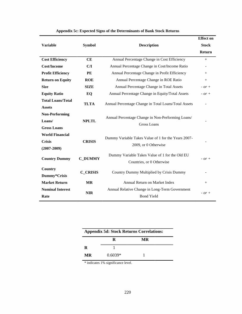
220

Appendix 5c: Expected Signs of the Determinants of Bank Stock Returns

Variable Symbol Description

Effect on

Stock

Return

Cost Efficiency CE Annual Percentage Change in Cost Efficiency +

Cost/Income C/I Annual Percentage Change in Cost/Income Ratio -

Profit Efficiency PE Annual Percentage Change in Profit Efficiency +

Return on Equity ROE Annual Percentage Change in ROE Ratio +

Size SIZE Annual Percentage Change in Total Assets - or +

Equity Ratio EQ Annual Percentage Change in Equity/Total Assets - or +

Total Loans/Total

Assets TLTA Annual Percentage Change in Total Loans/Total Assets -

Non-Performing

Loans/

Gross Loans

NPLTL Annual Percentage Change in Non-Performing Loans/

Gross Loans -

World Financial

Crisis

(2007-2009)

CRISIS Dummy Variable Takes Value of 1 for the Years 2007-

2009, or 0 Otherwise -

Country Dummy C_DUMMY Dummy Variable Takes Value of 1 for the Old EU

Countries, or 0 Otherwise - or +

Country

Dummy*Crisis C_CRISIS Country Dummy Multiplied by Crisis Dummy -

Market Return MR Annual Return on Market Index +

Nominal Interest

Rate NIR

Annual Relative Change in Long-Term Government

Bond Yield - or +

Appendix 5d: Stock Returns Correlations:

R MR

R 1

MR 0.6039* 1

* indicates 1% significance level.

221

Appendix 6

Appendix 6a: Model (A) Regression Diagnostic Tests of STATA for Model (I)

Appendix 6a.1 Variance Inflation Factors

Appendix 6a.2 Breusch-Pagan/Cook-Weisberg Test for Heteroskedasticity

Appendix 6a.3 Wooldridge Test for Autocorrelation in Panel Data

Mean VIF 2.58

SIZE 1.04 0.958942

EQ 1.05 0.954504

CE 1.07 0.935755

C_DUMMY 2.31 0.432916

CRISIS 4.46 0.223990

C_CRISIS 5.57 0.179619

Variable VIF 1/VIF

Prob > chi2 = 0.2868

chi2(1) = 1.13

Variables: fitted values of CASR

Ho: Constant variance

Breusch-Pagan / Cook-Weisberg test for heteroskedasticity

Prob > F = 0.3241

F( 1, 98) = 0.982

H0: no first-order autocorrelation

Wooldridge test for autocorrelation in panel data

222

Appendix 6a.4 Hausman Test

Appendix 6b: Model (A) Regression Diagnostic Tests of STATA for Model (II)

Appendix 6b.1 Variance Inflation Factors

Prob>chi2 = 0.4508

= 4.72

chi2(5) = (b-B)'[(V_b-V_B)^(-1)](b-B)

Test: Ho: difference in coefficients not systematic

B = inconsistent under Ha, efficient under Ho; obtained from xtreg

b = consistent under Ho and Ha; obtained from xtreg

C_CRISIS -.2882035 -.2290447 -.0591588 .0484683

CRISIS .0501691 -.0023407 .0525097 .0426874

EQ .5461016 .5388809 .0072207 .0419825

SIZE .2671845 .320165 -.0529805 .0680074

CE -1.118107 -.7447698 -.373337 .2065682

fe re Difference S.E.

(b) (B) (b-B) sqrt(diag(V_b-V_B))

Coefficients

Mean VIF 2.54

SIZE 1.07 0.935906

CI 1.07 0.934748

EQ 1.07 0.934228

C_DUMMY 2.31 0.433212

CRISIS 4.30 0.232473

C_CRISIS 5.40 0.185323

Variable VIF 1/VIF

223

Appendix 6b.2 Breusch-Pagan/Cook-Weisberg Test for Heteroskedasticity

Appendix 6b.3 Wooldridge Test for Autocorrelation in Panel Data

Appendix 6b.4 Hausman Test

Prob > chi2 = 0.0042

chi2(1) = 8.20




Prob > F = 0.3404

F( 1, 98) = 0.918



Prob>chi2 = 0.1253

= 8.62

chi2(5) = (b-B)'[(V_b-V_B)^(-1)](b-B)




C_CRISIS -.2248541 -.1835484 -.0413057 .04202

CRISIS .0325842 -.0096613 .0422455 .0374619

EQ .4569052 .4526574 .0042478 .0377799

SIZE .1298512 .2087653 -.0789141 .0628072

CI -.7165126 -.5912543 -.1252583 .0484796



Coefficients

224

Appendix 6c: Model (A) Regression Diagnostic Tests of STATA for Model (III)

Appendix 6c.1 Variance Inflation Factors

Appendix 6c.2 Breusch-Pagan/Cook-Weisberg Test for Heteroskedasticity

Appendix 6c.3 Wooldridge Test for Autocorrelation in Panel Data

Mean VIF 2.62

EQ 1.04 0.958830

SIZE 1.07 0.934448

PE 1.20 0.835861

C_DUMMY 2.34 0.427132

CRISIS 4.61 0.216907

C_CRISIS 5.45 0.183605

Variable VIF 1/VIF

Prob > chi2 = 0.0117

chi2(1) = 6.35




Prob > F = 0.2227

F( 1, 98) = 1.506



225

Appendix 6c.4 Hausman Test

Appendix 6d: Model (A) Regression Diagnostic Tests of STATA for Model (IV)

Appendix 6d.1 Variance Inflation Factors

Prob>chi2 = 0.8704

= 1.84

chi2(5) = (b-B)'[(V_b-V_B)^(-1)](b-B)




C_CRISIS -.2552257 -.2185322 -.0366934 .0489655

CRISIS .0539911 .0199035 .0340876 .0476641

EQ .5189983 .5196699 -.0006716 .0431439

SIZE .291924 .3593704 -.0674464 .0702085

PE .6559583 .7493524 -.0933941 .2144413



Coefficients

Mean VIF 2.52

ROE 1.02 0.976873

SIZE 1.04 0.958813

EQ 1.06 0.942101

C_DUMMY 2.31 0.432216

CRISIS 4.29 0.232985

C_CRISIS 5.40 0.185193

Variable VIF 1/VIF

226

Appendix 6d.2 Breusch-Pagan/Cook-Weisberg Test for Heteroskedasticity

Appendix 6d.3 Wooldridge Test for Autocorrelation in Panel Data

Appendix 6d.4 Hausman Test

Prob > chi2 = 0.4186

chi2(1) = 0.65




Prob > F = 0.2719

F( 1, 98) = 1.221



Prob>chi2 = 0.8406

= 2.06

chi2(5) = (b-B)'[(V_b-V_B)^(-1)](b-B)




C_CRISIS -.2325727 -.1965999 -.0359727 .0480581

CRISIS -.0006079 -.0345954 .0339875 .0426163

EQ .5285856 .5243346 .004251 .0430843

SIZE .2553244 .3135447 -.0582203 .0704639

ROE -6.69e-06 .0001306 -.0001372 .0002568



Coefficients

227

Appendix 6e: Model (B) Regression Diagnostic Tests of STATA

Appendix 6e.1 Variance Inflation Factors

Appendix 6e.2 Breusch-Pagan/Cook-Weisberg Test for Heteroskedasticity

Appendix 6e.3 Wooldridge Test for Autocorrelation in Panel Data

Mean VIF 1.00

NIR 1.00 0.997198

MR 1.00 0.997198

Variable VIF 1/VIF

Prob > chi2 = 0.0000

chi2(1) = 42.94




Prob > F = 0.0096

F( 1, 98) = 6.985



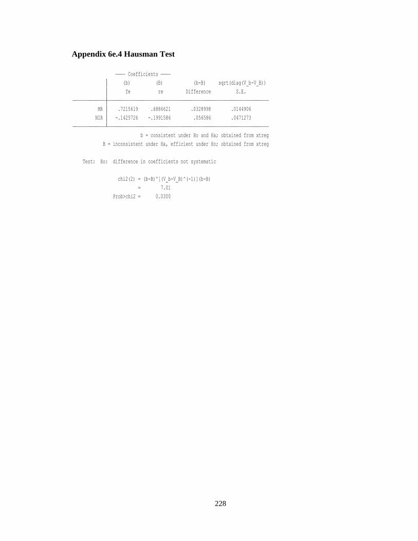
228

Appendix 6e.4 Hausman Test

Prob>chi2 = 0.0300

= 7.01

chi2(2) = (b-B)'[(V_b-V_B)^(-1)](b-B)




NIR -.1425726 -.1991586 .056586 .0471273

MR .7215619 .6886621 .0328998 .0144906



Coefficients

229

Bibliography

Adenso-Diaz, B. and Gascon, F. (1997), “Linking and Weighting Efficiency Estimates with Stock

Performance in Banking Firms”, Wharton school working paper, 97/21.

Afriat, S. N. (1972), “Efficiency Estimation of Production Functions”, International Economic

Review, 13 (3), 568-598.

Aftab, M., Ahamad, S., Ullah, W. and Sheikh, R.A. (2011), “The Impact of Bank Efficiency on

Share Performance: Evidence from Pakistan”, African Journal of Business Management,

5(10), 3975-3980.

Aigner, D. J., Lovell, C.A.K. and Schmidt, P. (1977), “Formulation and Estimation of Stochastic

Frontier Production Function Models”, Journal of Econometrics, 6, 21-37.

Al-Abadi, M.I. and Al-Sabbagh, O.W. (2006), “Interest Rate Sensitivity, Market Risk, Inflation,

and Bank Stock Returns”, Journal of Accounting, Business and Management, 13, 25-38.

Ali, A.I. and Seiford, L.M. (1993), “The Mathematical Programming Approach to Efficiency

Analysis”, in Fried, H.O., Lovell, C.A.K, and Schmidt, S.S. (EDS), The Measurement of

Productive Efficiency: Techniques and Applications, New York: Oxford University Press,

120-159.

Allen, L. and Rai, A. (1996), “Operational Efficiency in Banking: An International Comparison”,

Journal of Banking and Finance, 20, 655-672.

Allen, W. A. and Moessner, R. (2012), “The liquidity consequences of the euro area sovereign

debt crisis”, BIS Working Paper, No. 390.

Altunbas, Y., Liu, M. H., Molyneux, P. and Seth, R. (2000), “Efficiency and Risk in Japanese

Banking”, Journal of Banking and Finance, 24, 1605–1628.

Altunbas, Y., Gardener, E.P.M., Molyneux, P., and Moore, B. (2001a), “Efficiency in European

Banking”, European Economic Review, 45, 1931-1955.

Altunbas, Y., Evans, L. and Molyneux, P. (2001b) “Bank Ownership and Efficiency”, Journal of

Money, Credit, and Banking, 33(4), 926-954.

Altunbas, Y., Carbo, S., Gardener, E.P.M. and Molyneux, P. (2007), “Examining the

Relationships between Capital, Risk, and Efficiency in European Banking”, European

Financial Management, 13(1), 49-70.

230

Altunbas, Y., Gambacorta, L. and Marques-Ibanez, D. (2009), “Bank Risk and Monetary Policy”,

Working Paper No, 1075, European Central Bank.

Altunbas, Y., Manganelli, S. and Marques-Ibanez, D. (2011). “Bank Risk During the Financial

Crisis: DO business Models Matter?”. ECB Working Paper, No.1394, European Central

Bank, Frankfurt.

Arellano, C., Conesa, J. and Kehoe, T.J. (2012), “Chronic Sovereign Debt Crises in the Eurozone,

2010-2012”, Region (10453369), 4-11.

Arnold, G. (2008), “Corporate Financial Management”, Harlow: Financial Times Prentice Hall.

Athanasoglou, P. Delis, M. and Staikouras, C. (2006), “Determinants of Bank Profitability in the

Southern Eastern European Region”, Bank of Greece Working Paper, No. 47.

Ball, R. and Kothari, S.P. (1994), “Financial Statement Analysis”, New York, NY: Mc-Graw Hill.

Baltagi, B. H. (2005), “Econometric analysis of panel data”, Chichester: John Wiley&Sons Ltd.

Banker, R.D., Charnes, A. and Cooper, W.W. (1984), “Some Models for Estimating Technical

and Scale Inefficiencies in Data Envelopment Analysis”, Management Science, 30, 1078-

1092.

Basle Committee on Banking Supervision. (2000), “Principles for the Management of Credit

Risk”, September, http://www.bis.org/publ/bcbs75.pdf.

Battese, G. E. and Corra G. S. (1977), “Estimation of a production frontier model: with

application to the pastoral zone of Eastern Australia”, Australian Journal of Agricultural

Economics, 21, 169-79.

Battese, G. E. and Coelli T. J. (1988), “Prediction of Firm Level Technical Inefficiencies with a

Generalised Frontier Production Function and Panel Data”, Journal of Econometrics, 38,

387-399.

Battese, G. E. and Coelli, T. J. (1992), “Frontier Production Function, Technical Efficiency and

Panel Data: With Application to Paddy Farmers in India”, Journal of Productivity Analysis,

3, 153-169.

Battese, G. E. and Coelli, T. J. (1995), “A Model for Technical Inefficiency Effects in a Stochastic

Frontier Production Function for Panel Data”, Empirical Economics, 20, 325–332.

Battilossi, S. (2009), “Did Governance Fail Universal Banks? Moral Hazard, Risk Taking, and

Banking Crises in Interwar Italy”, Economic History Review, 62, 101-134.

http://www.bis.org/publ/bcbs75.pdf

231

Bauer, P.W., Berger, A.N, and Humphrey, D.B. (1993), “Efficiency and Productivity Growth in

US Banking”, In Fried,H.O., Lovell, C.A.K. and Schmidt, S.S., The Measurement of

Productive Efficiency. Oxford: University Press.

Bauer, P. W. and Hancock, D. (1993), “The Efficiency of the Federal Reserve in Providing Check

Processing Services”, Journal of Banking and Finance, 17(2/3), 287-311.

Bauer, P.W., Berger, A., Ferrier, G. and Humphrey, D. (1998), “Consistency conditions for

regulatory analysis of financial institutions: A comparison of frontier efficiency methods”,

Journal of Economics and Business, 50(2), 85–114.

Baum, C.F. (2006), “An Introduction to Modern Econometrics Using Stata”, College Station,

Tex.: Stata.

Baye, M.R. (2002), “Managerial Economics and Business Strategy”, London: Irwin McGraw-Hill.

Beccalli, E., & Frantz, P. (2009), “M&A operations and performance in banking”, Journal of

Financial Services Research, 36(2–3), 203–226.

Becalli, E., Casu, B. and Girardone, C. (2006), “Efficiency and Stock Performance in European

Banking”, Journal of Business Finance and Accounting, 33(1), 245-262.

Beggs, J. J. (1988), "Diagnostic Testing in Applied Econometrics", Economic Record, 64, 81-101.

Beirne, J., Caporale, G.M. and Spagnolo, N. (2009), “Market, Interest Rate and Exchange Rate

Risk effects on Financial Stock Returns: A GARCH-M Approach”, Quantitative and

Qualitative Analysis in Social Sciences”, 3(2), 44-68.

Berg, S.A., Førsund, F.R., Hjalmarsson, L. and Suominen, M. (1993), “Banking Efficiency in the

Nordic Countries” Journal of Banking and Finance, 17, 371-388.

Berger, A. N. (1993), “Distribution-free Estimates of Efficiency in the US Banking Industry and

Tests of the Standard Distributional Assumptions”, Journal of Productivity Analysis, 4,

261-292.

Berger, A. N. (1995), “The Profit-Structure Relationship in Banking-Tests of Market-Power and

Efficient-Structure Hypotheses”, Journal of Money, Credit and Banking, 27, 404-431.

Berger, A.N. and De Young, R. (1997), “Problem Loans and Cost Efficiency in Commercial

Banks”, Journal of Banking and Finance, 21, 849-870.

232

Berger, A.N. and Hannan, T.H. (1998), “The Efficiency Cost of Market Power in the Banking

Industry: A test of the “Quiet Life” and Related Hypotheses”, The Review of Economics and

Statistics, 80(3), 454-465.

Berger A. and Humphrey D. (1991), "The Dominance of Inefficiencies over Scale and Product

Mix Economies in Banking", Journal of Monetary Economics, 28, 117-148.

Berger, A. N. and Humphrey, D. B. (1992), “Measurement and efficiency issues in commercial

banking, in Output Measurement in the Service Sectors (Ed.) Z. Griliches, The University

of Chicago Press, Chicago, 245–479.

Berger, A. N. and Humphrey, D.B. (1997), “Efficiency of Financial Institutions: International

Survey and Directions for Future Research”, European Journal of Operation Research, 98,

175-212.

Berger, A.N. and Mester, L.J. (1997), “Inside the black box: What Explains Differences in the

Efficiencies of Financial Institutions”, Journal of Banking and Finance, 21 (7), 895-947.

Berger, A.N. and Mester, L.J. (1999), “What explains the dramatic changes in cost and profit

performance of the US banking industry?”, Working paper, 99-10, The Wharton School,

University of Pennsylvania.

Berger, A.N., Leusner, J.H. and Mingo, J.J. (1997), “The efficiency of bank branches”, Journal of

Monetary Economics, 40,141-162.

Berger, A.N., DeYoung, R., Genay, H. and Udell, G.F. (2000), “The globalization of Financial

Institutions: Evidence from cross-border banking performance”, Brookings-Wharton Papers

on Financial Services, 3, 23-158.

Blinder, A. S. (2009), “Crazy Compensation and the Crisis”, The Wall Street Journal, 28 May,

A15.

Bloem, A. M. and Freeman, R. (2005), “The Treatment of Nonperforming Loans”, Issue Paper

Prepared for the July 2005 Meeting of the Advisory Expert Group on National Accounts,

June 2005, International Monetary Fund.

Blundell-Wignall, A. and Atkinson, P. (2009), “Origins of the Financial Crisis and Requirements

for Reform”, Journal of Asian Economics, 20, 536-548.

Boles, J. N. (1966), “Efficiency Squared – Efficient Computation of Efficiency Indexes”,

Proceeding of the Thirty Ninth Annual Meeting of Western Farm Economics Association,

137-142.

233

Bonin, J. Hassan, I., and Wachtel, P. (2005), “Bank performance, efficiency and ownership in

transition countries”, Journal of Banking and Finance, 29, 31-53.

Brealey, R. A. and Myers, S.C. (1991), “Principles of Corporate Finance”, New York, NY:Mc-

Graw Hill.

Breusch, T. S. and A. R. Pagan (1979), "A Simple Test for Heteroskedasticity and Random

Coefficient Variation", Econometrica, 47, 1287-1294.

Brewer, E., III, and C. F. Lee (1990), “An Intracyclical Analysis of the Risk Sensitivity of Bank

Stock Returns”, Quarterly Journal of Business and Economics, 29, 125-143.

Brown, P., Kleidon, A.W. and Marsh, T.A. (1983), “New Evidence on the Nature of Size-Related

Anomalies in stock Prices”, Journal of Financial Economies, 12, 33-56.

Brunnermeier, M.K. (2009), “Deciphering the Liquidity and Credit Crunch 2007-2008”, Journal

of Economics Perspective, 23(1), 77-100.

Cade, E. (1997), "Managing Banking Risks", Cambridge: Gresham Books.

Calomiris, C. W. (2009), ‘‘Financial Innovation, Regulation, and Reform’’, Cato Journal, 29 (1),

65‐92.

Calverley, J.P. (2009), “When Bubbles Burst: Surviving the Financial Fallout”, London: Nicholas

Brealey Publishing.

Canhoto, A. and Dermine, J. (2003), “A Note on Banking Efficiency in Portugal, New VS. Old

banks”, Journal of Banking and Finance, 27, 2087-2098.

Caprio, G., Demirguc-Kunt, A. and Kane, E.J. (2010), “The 2007 Meltdown in Structured

Securitization: Searching for Lessons not Scapegoats”, The World Bank Research, 25(1),

125-155.

Carbo´ , S., Fernandez, F. (2005), “The determinants of bank margins: The effects of

diversification”, FUNCAS, working paper.

Carbo, S., Gardener, E.P.M. and Williams, J. (2002), “Efficiency in Banking: Empirical Evidence

from the Savings Banks Sector”, Manchester School 70, 204-228.

Carmassi, J., Gros, D. and Micossi, S. (2009), “The Global Financial Crisis: Causes and Cures”.

JCMS, 47(5), 977-996.

Casu, B. and Girardone, C. (2006), “Bank Competition, Concentration and Efficiency in the

Single European Market”, The Manchester School, 74 (4), 441-468.

234

Casu, B. and Girardone, C. (2010), “Integration and Efficiency Convergence in EU Banking

Markets”, Omega, 38, 260-267.

Casu, B., Girardore, C. and Molyneux, P. (2006), “Introduction to Banking”, Essex: Pearson.

Chalfant, J. A. and Gallant A.R. (1985), “Estimating substitution elasticities with the Fourier cost

function”, Journal of Econometrics, 28, 205-222.

Chan, L.K., Hamao, Y. and Lakonishok, J. (1991), “Fundamentals and Stock Returns in Japan”,

Journal of Finance, 46, 1739-1789.

Chan, S.G. and Abd Karim, M.Z. (2010), “Bank efficiency, profitability and equity capital:

evidence from developing countries”, American J. of Finance and Accounting, 2(2), 181 -

195.

Charnes, A., Cooper, W.W., and Rhodes, E. (1978), "Measuring Efficiency of Decision Making

Units", European Journal of Operational Research, 2, 429-444.

Chen, Y. K., Kao, L. F., Shen, C. H. and Yeh, C. Y. (2010), “Bank liquidity risk and

performance”, International Monetary Fund, Working Paper.

Christensen, R.L., Jorgenson, D.W. and Lau. L.J. (1971), “Conjugate Duality and the

Transcendental Logarithmic Production Function”, Econometrics, 39, 225-256.

Christensen, R.L., Jorgenson, D.W. and Lau. L.J. (1973), “Transcendental Logarithmic Production

Frontiers”, The Review of Economics and Statistics, 55, 28-45.

Chu, S.F. and Lim, H. (1998), “Share performance and profit efficiency of banks in an

ologopolistic market: evidence from Singapore”, Journal of Multinational Financial

Management, 8,155–168.

Claessens, S., Dasgupta, S. and Glen, J. (1998), “The Cross-Section of Stock Returns: Evidence

From Emerging Markets”, Emerging Markets Quarterly, 2, 4-13.

Claessens, S. and Kose, M.A. (2010), “The Financial Crisis of 2008-2009: Origins, Issues, and

Prospects”, Journal of Asian Economics, 21, 239-241.

Coelli, T. J., Rao, D. S. P. O’Donnel, C.J.,and Battese, G. E. (2005), “An Introduction to

Efficiency and Productivity Analysis”, 2nd

ed., London: Springer.

Cook, R.D. and Weisberg, S. (1983), “Diagnostics of Heteroscedasticity in Regression”,

Biometrika, 70, 1-10.

http://www.inderscience.com/browse/index.php?journalID=229&year=2010&vol=2&issue=2

http://www.inderscience.com/browse/index.php?journalID=229&year=2010&vol=2&issue=2

235

Cornwell, C., Schmidt, P. and Sickles, R. C. (1990), “Production Frontiers with Cross-sectional

and Time-series Variation in Efficiency Levels”, Journal of Econometrics, 46, 185-200.

De Borger, B., Kerstens, K., Moesen, W. and Vanneste, J. (1994), “A non-parametric Free

Disposal Hull (FDH) approach to technical efficiency: an illustration of radial and graph

efficiency measures and some sensitivity results”, Swiss Journal of Econometrics and

Statistics, 130(4), 647-667.

Debreu, G. (1951), “The Coefficient of Resource Utilisation”, Econometrica, 19 (3), 273-292.

Demirguc-Kunt, A. and Serven, L. (2010), “Are All the Sacred Cows Dead? Implications of the

Financial Crisis for Macro-and Financial Policies”, World Bank Research Observer, 25(1),

91-124.

Demsetz, H., (1973), “Industry structure, market rivalry, and public policy”, Journal of Law and

Economics 16, 1-9.

Demsetz, H., (1974), “Two Systems of Belief about Monopoly”, in Goldschmid H.J., Mann H.M.

and J.F. Weston (eds), Industrial Concentration: The New Learning, 164-184, Boston:

Little Brown.

Demyanyk, Y. and Hasan, I. (2010), “Financial Crises and Bank Failures: A review of Prediction

Methods”, Omega, 38 (5), 315-324.

Deprins, D., Simar, L. and Tulkens, H. (1984), “Measuring labor inefficiency in post offices”, In

the Performance of Public Enterprises: Concepts and Measurements (M. Marchand, P.

Pestieau and H. Tulkens, eds.) 243–267. Amsterdam: North-Holland.

Dermine, J. (2006), “European banking integration: don’t put the cart before the horse”, Financial

Institutions, Markets and Money”, 15, 57-106.

Di, Iorio, A., Faff, R. and Sander, H. (2006), “An Investigation of the Interest Rate Risk and the

Exchange Rate Risk of the European Financial Sector: Euro Zone versus Non-euro Zone

Countries”, Mimeo.

Diamond, D.W. and Rajan, R. (2009), "The Credit Crisis: Conjectures about Causes and

Remedies", American Economic Review, Papers and Proceedings: 99: 606-10.

Dietsch, M. and Lozano-Vivas, A. (2000), “How the Environment Determines Banking

Efficiency: A Comparison between French and Spanish Industries”, Journal of Banking and

Finance, 24, 985-1004.

236

Drake, L. (2001), “Efficiency and productivity change in UK banking”, Applied Financial

Economics, 11, 557-571.

Eastwood, B.J. and Gallant A.R. (1991), “Adaptive rules for semi-nonparametric estimators that

achieve asymptotic normality”, Economic Theory, 7, 307-340.

Eisenbeis, R. A, Ferrier, G. D and Kwan, S. H. (1999), “The informativeness of stochastic frontier

and programming frontier efficiency scores: cost efficiency and other measures of bank

holding company performance”, Federal Reserve Bank of Atlanta, Working paper, p. 99–

23.

Eisenbeis, R.A. (2010), “The Financial Crisis: Miss-Diagnosis and Reactionary Responses”,

Atlantic Economic Journal, 38, 283-294.

Eiteman, D.K., Stonehill, A.I. and Moffett, M.H. (2009), “Multinational Business Finance”,

Harlow: Pearson Education.

El-Agraa, A.M. (2000), “The European Union: Economics and Policies”, London: Prentice Hall

Europe.

Elbadawi, I., Gallant, A.R. and Souza G. (1983), “An elasticity can be estimated Consistently

without a priori knowledge of functional form”, Econometrica, 51, 1731-1753.

Enoch, C., Marston, D. and Taylor. M. (2002), “Building Strong Banks: Through Surveillance and

Resolution”, Washington DC: International Monetary Fund.

Eubanks, W.W. (2010a), “The status of the Basel III Capital Adequacy Accord”, Congressional

Research Service, 7–5700. www.crs.gov, R41467.

Eubanks, W.W. (2010b), “The European Union’s Response to the 2007-2009 Financial Crisis”,

Congressional Research Service, 7–5700. www.crs.gov, R41367.

European Central Bank (ECB), (2005), “Banking structures in the New EU Member States”,

European Central Bank.

European Central Bank (ECB), (2008), “EU Banking Structures”, October.

European Central Bank (ECB), (2010a), “EU Banking Structures”, September.

European Central Bank (ECB), (2010b), “Financial Integration in Europe”, April.

European Council (1993), “Presidency Conclusions, Copenhagen European Council”, Bulletin of

the EC 21-22 June; Europe Documents. No.1844/45, 24.06.1993.

237

Fama, E. F. and French, K. R. (1992), “The Cross-Section of Expected stock Returns”, Journal of

Finance, 47(2), 427-465.

Fama, E. F. and French, K. R. (1993), “Common Risk Factors in the Returns on Stocks and

Bonds”, Journal of Financial Economics, 33, 3-56.

Färe, R., Grosskopf, S. and Logan, J. (1983), “The relative efficiency of Illinois Electric Utilities”,

Resources and Energy, 5, 349-367.

Färe, R., Grosskopf, S. and Lovell, C.A.K. (1985), “The Measurement of Efficiency of

Production”, Boston: Kluwer Academic Publishers.

Farrell, M. J. (1957), “The measurement of Productive Efficiency”, Journal of the Royal

Statistical Society, 120, 253-90.

Fethi, M.D. and Pasiouras, F. (2010), “Assessing Bank Efficiency and Performance with

Operational Research and Artificial Intelligence Techniques: A Survey”, European Journal

of Operational Research, 204 (2), 189-198.

Fiordelisi, F., Marques-Ibanez, D., & Molyneux, P. (2011), “Efficiency and Risk in European

Banking”, Journal of Banking & Finance, 35(5), 1315-1326.

Flannery, M. J. and James, C. M. (1984), “The Effect of Interest Rate Changes on the Common

Stock Returns of Financial Institutions”, The Journal of Finance, 39, 1141-1153.

Forbes, K. and Rigobon, R. (2002), “No Contagion, only Interdependence: Measuring Stock

Market Comovements”, Journal of Finance, 57 (5), 2223-2261.

Fries, S., and Taci, A. (2005), “Cost efficiency of banks in transition: Evidence from 289 banks in

15 post-communist countries”, Journal of Banking and Finance, 29, 55-81.

Gallant, A.R. (1981), “On the bias in flexible functional forms and essentially unbiased form: The

Fourier flexible form”, Journal of Econometrics, 15, 211-245.

Gallant, A.R. (1982), “Unbiased determination of production technologies”, Journal of

Econometrics, 20, 285-324.

Gallant, A.R. and Souza G. (1991), “On the asymptotic normality of Fourier Flexible form

estimates”, Journal of Econometrics, 50, 329-353.

GAO. (2010), “Financial Markets Regulation: Financial Crisis Highlights Need to Improve

Oversight of Leverage at Financial Institutions and across System”, GAO-10-555T.

238

Gardener E.P.M. (1991), "Capital Adequacy in the New Europe", Research Papers in Banking

and Finance, Institute of European Finance, Bangor, No. 13.

Gardener E.P.M. (1992), "Capital Adequacy after 1992: The Banking Challenge", Research

Papers in Banking and Finance, Institute of European Finance, Bangor, No. 11.

Gathon, H. J. and Perelman, S. (1992), “Measuring Technical Efficiency in European Railways: A

Panel Data Approach”, Journal of Productivity Analysis, 3(1/2), 135-151.

Girard, E., Nolan, J., and Pondillo, T. (2010), “DETERMINANTS OF EMERGING MARKETS'

COMMERCIAL BANK STOCK RETURNS”, Global Journal Of Business Research

(GJBR), 4 (2), 11-26.

Girardone, C. Molyneux, P. and Gardener, E.P.M. (2004), “Analysing the Determinants of Bank

Efficiency: The Case of Italian Banks”, Applied Economics, 36 (3), 215-227.

Godfrey, L. G. (1978), “Testing for Multiplicative Heteroscedasticity”, Journal of Econometrics,

8, 227-236.

Gong, B.-H. and Sickles, R.S. (1989), “Finite Sample Evidence on the Performance of Stochastic

Frontier Models Using Panel Data”, Journal of Productivity Analysis, 1(3), 229-261.

Greene, W. H. (2008), “Econometric Analysis”, 6th ed., Upper Saddle River, NJ: Pearson Prentice

Hall.

Greuning, H.V. and Bratanovic, S.B. (2009), “Analyzing and Managing Banking Risk: a

Framework for Assessing Corporate Governance and Financial Risk”, Washington D.C:

The World Bank.

Grier, W.A. (2007), “Credit Analysis of Financial Institutions”, 2nd

ed., London: Euromoney

Institutional Investor Plc.

Grigorian, D. and Manole, V. (2002), “Determinants of Commercial Bank Performance in

Transition: An Application of Data Envelopment Analysis”, IMF WP/146.

Gujarati, D. N. and Porter, D. C. (2009), “Basic Econometrics”, London : McGraw-Hill.

Gup, B.E. (2001), “Banking and Financial Institutions: A Guide for Directors, Investors, and

Borrowers”, New Jersey: John Wiley & Sons.

239

Hadad, M. D., Hall, M. J. B., Kenjegalieva, K., Santoso, W. and Simper, R. (2011), “Banking

Efficiency and Stock Market Performance: An Analysis of Listed Indonesian Banks”,

Review of Quantitative Finance and Accounting, 37(1), 1-20.

Haldane, A. G. (2009), “Why Banks Failed the Stress Test”, Speech at Marcus-Evans Conference

on Stress Testing, 9–10 February.

Halkos, G.E. and Salamouris, D.S. (2004), “Efficiency measurement of the Greek commercial

banks with the use of financial ratios: a data envelopment analysis approach”, Management

Accounting Research, 15, 201-224.

Hänsel, D. and Krahnen J.P. (2007), “Does Credit Securitization Reduces Bank Risk? Evidence

from the European CDO Market”, mimeo, Goethe-University Frankfurt.

Hanson, J. A. and Rocha, R.D.R. (1986), "High Interest Rates, Spreads, and the Cost of

Intermediation: Two Studies", Industry and Finance Series 18, World Bank, Industry

Department, Washington, D.C.

Haq, M. and Heaney, R. (2009), “European Bank Equity Risk: 1995-2006”, Journal of

International Financial Markets, Institutions & Money, 19, 274-288.

Hasan, I. And Morton, K. (2003), “Development and efficiency of the banking sector in a

transitional economy: Hungarian experience”, Journal of Banking and Finance, 27, 2249-

2271.

Hasenkamp, G. (1976), “Specification and Estimation of Multiple-Output Production Functions”,

New York: Springer-Verlag.

Havrylchyk, O. (2006), “Efficiency of the Polish banking industry: Foreign versus domestic

banks”, Journal of Banking and Finance, 30, 1975-1996.

He, L., & Reichert, A. (2003), “Time variation paths of factors affecting financial institutions

stock returns”, Atlantic Economic Journal, 31, 71–86.

Heffernan, S. (1996), “Modern Banking in Theory and Practice”, Chichester: John Wiley & Sons.

Hollo, D. And Nagy, M. (2006), “Bank Efficiency in the Enlarged European Union”, BIS Papers

No.28, August, 217-235.

Howells, P. and Bain, K. (2008), “The Economics of Money, Banking and Finance, a

European Text”, Harlow: Prentice Hall Financial Times.

Hsiao, C. (2003), “Analysis of Panel Data”, Cambridge: Cambridge University Press.

http://www.springerlink.com/content/0924-865x/

240

Hsiao, C. (2006), “Panel Data Analysis – Advantages and Challenges”, IEPR Working Paper No.

06.49. Available at SSRN: http://ssrn.com/abstract=902657.

Hull, J.C. (2010), “Risk Management and Financial Institutions”, Boston: Pearson.

Hunter, G. (2008), “Anatomy of the 2008 Financial Crisis: An Economic Analysis Postmortem”,

Working paper.

Hunter, W.C. and Timme, S.G. (1986), “Technical Change, Organizational Form, and the

Structure of Bank Production”, Journal of Money, Credit and Banking, 18(2), 152-166.

Hwang, I., In, F.H. and Kim, T. (2010), “Contagion Effects of the US Subprime Crisis on

International Stock Markets”, Mimeo.

International Monetary Fund. (2000), “Transition Economies: An IMF Perspective on Progress

and Prospects”. Accessed 28/6/2012

http://www.imf.org/external/np/exr/ib/2000/110300.htm

Ioannidis, C., Molyneux, P. and Pasiouras, F. (2008), “The relationship between bank efficiency

and stock returns: evidence from Asia and Latin America”, University of Bath (UK), School

of Management, Working Paper Series 2008.10.

Isik, I. and Hassan, M. k. (2003), “Efficiency, Ownership and Market Structure, Control and

Governance in Turkish Banking Industry”, Journal of Business Finance and Accounting, 30

(9/10), 1363-1421.

Isik, I. and Hassan, M. k. (2002), “Cost and Profit Efficiency of the Turkish Banking Industry: An

Empirical Investigation”, The Financial Review, 37, 257-280.

Jaccard, J. (2001), “Interaction Effects in Logistic Regression”, London: Sage Publications.

Jagtiani, J. and A. Khanthavit, (1996), “Scale and scope economies at large banks: Including off-

balance sheet products and regulatory effects (1984-1991)”, Journal of Banking and

Finance, 20 (7), 1271-1287.

Jemric, I. And Vujcic, B. (2002), “Efficiency of Banks in Croatia: A DEA Approach”, Croatian

National Bank Working Papers, W-7, Croatian National Bank, Zagreb.

Jondrow, J., Lovell, C., Materov, I., & Schmidt, P. (1982), “On the estimation of technical

efficiency in the stochastic frontier production function model”, Journal of Econometrics,

19, 233−238.

http://ssrn.com/abstract=902657

http://www.imf.org/external/np/exr/ib/2000/110300.htm

241

Jorion, P. (1997), “Value at Risk: The New Benchmark for Controlling Market Risk", New York:

McGraw-HilL.

Kablan, S. (2010), “Banking efficiency and Financial Development in Sub-Saharan Africa”, IMF

Working Paper series WP/10/136 International Monetary Fund.

Kane, E. J., and Unal, H. (1988), “Change in Market Assessment of Deposit Institution riskiness”,

Journal of Financial Services Research, 1, 207–228.

Kasman, S., Vardar, G. and Tunc, G. (2011), “The Impact of Interest Rate and Exchange Rate

Volatility on Banks’ Stock Returns and Volatility: Evidence from Turkey”, Economic

Modelling, 28, 1328-1334.

Kasman, A. and Yildirim, C. (2006), “Cost and Profit Efficiency in Transition Banking: The Case

of New EU Members”, Applied Economics, 38, 1079-1090.

Kendall, L.T. and Fishman, M.J. (2000), “A Primer on Securitization”, Cambridge, Mass: MIT

Press.

Keys, B., Mukherjee, T., Seru, A. and Vig, V. (2008), “Did Securitization Lead to Lax Screening?

Evidence from Subprime Loans”, Chicago GSB working paper.

King, P. and Tarbert, H. (2011), “Basel III: An Overview”, Banking & Financial Services Policy

Report, 30 (5), 1-18.

Kirkwood, J. and Nahm, D. (2006), “Australian banking efficiency and its relation to stock

returns”, The Economic Record, 82(258), 253–267.

Koetter, M. and Porath, D. (2007), “Efficient, Profitable and Safe Banking: An Oxymoron?

Evidence from a Panel VAR Approach”, SSRN Working Paper.

Koopmans, T. (1951), “Activity analysis of production and allocation”, John Wiley, New York.

Kosak, M. Zajc, P. and Zoric, J. (2009), “Bank Efficiency Differences in the New EU Member

States”, Baltic Journal of Economics, 9 (2), 67-90.

Kothari S.P. (2001), “Capital Market Research in Accounting”, Journal of Accounting and

Economics, 31, 105-231.

Kumbhakar, S. C. (1987), “The Specification of Technical and Allocative Inefficiency in

Stochastic Production and Profit Frontiers”, Journal of Econometrics, 34, 335-48.

Kumbhakar, S. C. (1990), “Production Frontiers, Panel Data, and Time-Varying Technical

Inefficiency”, Journal of Econometrics, 46(1/2), 201-212.

242

Kumbhakar, S.C., Ghost, S. and McGuckin, J.T. (1991), “A Generalized Production Frontier

Approach for Estimating Determinants of Inefficiency in Us Dairy Farms”, Journal of

Business and Economic Statistics, 9(3), 279-286.

Kumbhakar, S. and Lovell, C.A.K. (2000), “Stochastic Frontier Analysis”, Cambridge University

Press.

Kwan, S. H. (1991), “Re-examination of Interest Rate Sensitivity of Commercial Bank Stock

Returns Using a Random Coefficients Model”, Journal of Financial Services Research, 15,

61–76.

Laeven, L. (1999), “Risk and Efficiency in East Asian Banks”, World Bank Discussion Paper.

Lang, W. W., and Jagtiani, J.A. (2010), “The Mortgage and Financial Crises: The Role of Credit

Risk Management and Corporate Governance”, Atlantic Economic Journal, 38, 295-316.

Lee, F. C. and E. J. Finnerty, (1990), "Corporate Finance: Theory, Method and Application",

Orlando: Harcourt Brace Jovanovich.

Lee, Y.H. and Schmidt, P. (1993), “A Production Frontier Model with Flexible Temporal

Variation in Technical Inefficiency”, In Fried,H.O., Lovell, C.A.K. and Schmidt, S.S., The

Measurement of Productive Efficiency. Oxford: University Press.

Leibenstein, H. (1966), “Allocative efficiency vs. `X-efficiency'”, American Economic Review,

56, 392-415.

Leibenstein, H. (1978), "On the Basic Proposition of X-efficiency Theory", The American

Economic Review, 68 (2), 328.

Leibenstein, H. (1979), "X-Efficiency: From Concept to Theory", Challenge, 22 (4), 13-22.

Lensink, R., Meesters, A. and Naaborg, I. (2008), “Bank efficiency and foreign ownership: Do

good institutions matter?”, Journal of Banking and Finance, 32, 834-844.

Lepetit, L., Nys, E., Rous, P. and Tarazi, A. (2008), “Bank Income Structure and Risk: An

Empirical Analysis of European Banks”, Journal of Banking and Finance, 32, 1452-1467.

Liadaki, A. and Gaganis, C. (2010), “Efficiency and stock performance of EU banks: Is there a

relationship?”, Omega, 38, 254-259.

Lintner, J. (1965b), "The Valuation of Risk Assets and the Selection of Risky Investments in

Stock Portfolios and Capital Budgets", Review of Economics and Statistics, 47, 13-37.

243

Llewellyn, D. (1999), “The Economic Rational for Financial Regulation”, FSA Occasional Papers

in Financial Regulation, Occasional Paper Series 1.

Lovell, C.A.K. (1994), “Linear Programming Approaches to the Measurement and Analysis of

Productive Efficiency”, Top, 2, 175-248.

Lozano-Vivas, A., Pastor, J.T. and Pastor, J.M. (2002), “An Efficiency comparison of European

Banking Systems Operating under Different Environmental Conditions”, Journal of

Productivity Analysis, 18, 59-77.

Mamatzakis, E., Staikouras, C., and Koutsomanoli-Filippaki, A. (2008), “Bank efficiency in the

new European Union member states: Is There Convergence?”, International Review of

Financial Analysis, 17, 1156-1172.

Mankiw, N.G. (2011), “Principles of Macroeconomics”, Mason, OH: Thomson South-Western.

Martin-Oliver, A. and Saurina, J. (2007), “Why do Banks Securitize Assets?”, Working Paper,

Bank of Spain.

Mathieson, D. J. and Roldos, J. (2001), “Foreign Banks in Emerging Markets”, In Litan, R. E.,

Masson, P. and Pomerleano, M. (editors): Open Doors - Foreign Participation in Financial

Systems in Developing Countries. Washington DC: Brookings Institution Press, 15-55.

Matousek, R. and Taci, A. (2004), “Efficiency in Banking: Empirical Evidence from the Czech

Republic”, Economics of Planning, 37, 225-244.

Matz, L. and P. Neu (eds). (2007), “Liquidity Risk Measurement and Management: A

Practitioner’s Guide to Global Best Practices”, Singapore: John Wiley & Sons (Asia).

Maudos, J. and Fernandez de Guevara, J. (2004), “Factors explaining the interest margin in the

banking sectors of the European Union”, Journal of Banking and Finance 28, 2259–2281.

Maudos, J., Pastor, J.M. Perez, F. and Quesada, J. (2002a), “Cost and Profit Efficiency in

European Banks”, Journal of International Financial Markets, Institutions and Money,

12(1), 33-58.

Maudos, J., Pastor, J.M. & Perez, F. (2002b), “Competition and Efficiency in the Spanish Banking

Sector: The Importance of Specialization”, Applied Financial Economics, 12, 505-516.

McAllister, P. and McManus, D. (1993), “Resolving the Scale Efficiency Puzzle in Banking”,

Journal of Banking and Finance, 17, 389-406.

244

Meeusen, W. and Van Den Broeck, J. (1977), “Efficiency Estimation from Cobb-Douglas

Production Functions with Composed Error”, International Economic Review, 18(2), 435-

444.

Méon, P., & Weill, L. (2005), “Can Mergers in Europe Help Banks Hedge Against

Macroeconomic Risk?”, Applied Financial Economics, 15(5), 315-326.

Merrouche, O. and Nier, E. (2010), “What Caused the Global Financial Crisis? Evidence on the

Drivers of Financial Imbalances 1999-2007”, IMF working paper.

Merton, R.C. (1973), “An Intertemporal capital assets Pricing Model”, Econometrica, 41, 867-

887.

Merton, R.C. (1989), “On the application of the continuous – time theory of finance to financial

intermediation and insurance”, Geneva Papers on Risk and Insurance Theory, 14 (52), 225-

61.

Mester, L. (1996), “A study of bank efficiency taking into account risk-preferences”, Journal of

Banking and Finance, 20, 1025–1045.

Mishkin, F.S. and Eakins, S.G. (2012), “Financial Markets and Institutions”, Harlow: Pearson

Education.

Molyneux P., Altunbas Y., and E.P.M. Gardener. (1996), “Efficiency in European Banking”,

Chichester: John Wiley and Sons.

Monroe, M. (2010), “Basel III redefines capital”, ABA Banking Journal, 102(11), 33-35.

Munoz, M.P., Marquez, M.D. and Sanchez, J.A. (2011), “Contagion between United states and

European Markets during the Recent Crises”, The IEB International Journal of finance”, 2,

2-25.

Murillo-Zamorano, L. R. (2004), “Economic Efficiency and Frontier Techniques”, Journal of

Economic Surveys, 18, 1, 33-77.

Murry, M. P. (2006), “Econometrics: A Modern Introduction”, London: Pearson Addison Wesley.

Nelson, R.M., Belkin, P., Mix, D.E. and Weiss, M.A. (2012), “The Eurozone Crisis: Overview

and Issues for Congress”, Congressional Research Service, 7-5700.

Neri, S. and Ropele, T. (2013), “The macroeconomic effects of the sovereign debt crisis in the

euro area”, In Bank of Italy Workshops and Conferences The sovereign debt cisis and the

euro area.

245

O’Brennan, J. (2006), “The Eastern Enlargement of the European Union”, New York: Routledge.

OECD (2010), “Minimising Risks from Imbalances in European Banking”, OECD Economic

Surveys: Europ Area, 20, 121-159.

Oral, M. and Yolalan, R. (1990), “An Empirical Study on Measuring Operating Efficiency and

Profitability of Bank Branches”, European Journal of Operational Research, 46, 282-294.

Pasiouras, F., Liadaki, A. and Zopounidis, C. (2008), “Bank efficiency and share performance:

evidence from Greece”, Applied Financial Economics, 18, 1121-1130.

Pawlowska, M. (2003), “The Impact of M&A on Technical Efficiency, Scale Efficiency and

Productivity Change in the Polish Banking Sector: a Non-Parametric Approach”, Materialy

i Studia - Paper No. 29. Warsaw: National Bank of Poland, October 2003.

Petersen, M. (2009), “Estimating standard errors in Finance Panel Data Sets: Comparing

Approaches”, Review of Financial Studies, 22, 435-480.

Pilbeam, K. (2005), “Finance and Financial Markets”, Basingstoke: Palgrave Macmillan.

Pitt, M.M. and Lee, L.F. (1981), “Measurement and Sources of Technical Inefficiency in the

Indonesian Weaving Industry”, Journal of Development Economics, 9, 43-64.

Poole, W. (2010), “CAUSES AND CONSEQUENCES OF THE FINANCIAL CRISIS OF 2007-

2009”, Harvard Journal of Law & Public Policy, 33(2), 421-441.

Radic, N., Fiordelisis, F. and Girardone, C. (2012), “Efficiency and Risk-Taking in Pre-Crisis

Investment Banks”, Journal of Financial Services Research, 41, 81-101.

Resti, A. (1998), “Regulation Can Foster Mergers, Can Mergers Foster Efficiency? The Italian

Case”, Journal of Economics and Business, 50 (2), 157-169.

Revell, J. (1979), “Inflation and Financial Institutions”, Financial Times, London.

Rose, P.S. (1999), “Commercial Bank Management”, 4th ed, Irwin/McGraw-Hill.

Ross, S.A. (1976), “The Arbitrage Theory of Capital Asset Pricing”, Journal of Economic Theory,

343-62.

Sarafidis, V. (2002), “An Assessment of Comparative Efficiency Measurement Techniques”,

Europe Economics, Occasional Paper 2.

Saunders, A. and Cornett, M.M. (2006), “Financial Institutions Management: A Risk Management

Approach”, New York: McGraw-Hill.

246

Schmidt, P. and Sickles, R. C. (1984), “Production Frontiers and Panel Data”, Journal of Business

and Economic Statistics, 2, 367-374.

Sealey, C. W. and Lindley, J. T. (1977), “Inputs, Outputs, and a Theory of Production and Cost at

Depository Financial Institutions”, Journal of Finance, 32, 1251-1266.

Sensarma, R. and Jayadev, M. (2009), “Are Bank stocks Sensitive to risk Management?”, The

Journal of Risk finance, 10 (1), 7-22.

Sharpe, W. F., (1964), "Capital Asset Prices: A Theory of Market Equilibrium Under Conditions

of Risk", Journal of Finance, 19, 425-442.

Shephard, R. W. (1953), “Cost and Production Functions”, Princeton, Princeton University Press.

Shephard, R. W. (1970), “The Theory of Cost and Production Functions”, Princeton, Princeton

University Press.

Sherman, H.D. and Gold, F. (1985), “Bank Branch Operating Efficiency: Evaluation with Data

Envelopment Analysis”, Journal of Banking and Finance, 9(2), 297-315.

Shin, H.S. (2009). “Leverage, Securitization and Global Imbalances”, Working paper 5, Hong

Kong Institute for Monetary Research.

Shirai, S. (2009), “The Impact of the US Subprime Mortgage Crisis on the World and East Asia”,

Paper No.14722, 2 April. Munich Personal RePEc Archive.

Spatz, C. (2010), “Basic Statistics: Tales of Distributions”, Wadsworth Publishing Co Inc.

Spong, K., Sullivan, R.J. and DeYoung R. (1995), “What makes a bank efficient? – A look at

financial characteristics and bank management and ownership structure”, FRB of Kansas

City Review, December, 1-19.

Staikouras, C.K. and Koutsomanoli-Fillipaki, A. (2006), “Competition and Concentration in the

New European Banking Landscape”, European Financial Management, 12(3), 443-482.

Stone, B. (1974), “Systematic Interest Rate Risk in a Two-Index Model of Returns”, Journal of

Financial and quantitative Analysis, 9, 709-721.

Sufian, F. and Majid, M.Z.A. (2009), “Bank Efficiency and Share Prices in China: Empirical

Evidence from a Three-Stage Banking Model”, International Journal of Computational

Economics and Econometrics, 1, 23-47.

247

Sufian, F. and Majid, M.Z.A. (2007), “Banks’ Efficiency and Stock Prices in Emerging Markets:

Evidence from Malaysia”, Journal of Asia-Pacific Business, 7(4), 35-53.

Sun, L. and Change, T.P. (2011), “A Comprehensive Analysis of the Effects of Risk Measures on

Bank Efficiency”, Journal of Banking and Finance, 35, 1727-1735.

Tapiero, C.S. (2004), “Risk and Financial Management: Mathematical and Computational

Methods”, Chichester : John Wiley.

Taylor, J.B. (2008), “The Financial Crisis and the Policy Responses: An Empirical Analysis of

What Went Wrong”, Working paper.

Thomas, R. (2010), “The Role of Mortgage Securitisation in the Financial Crisis and How to

Restore the Market's Health”, Housing Finance International, 25(1), 19-24.

Tomova, M. (2005), “Efficiency of European Banking -Inequality and Integration”, Money Macro

and Finance Research Group, Volume 89.

Tulkens, H. (1986), "The performance approach in public sector economics: An introduction and

an example", Annales de l'économiepublique, sociale et cooperative 57(4), 429-443.

Tulkens, H. (1993), "On FDH Efficiency Analysis: Some Methodological Issues and Applications

to Retail Banking, Courts, and Urban Transit", Journal of Productivity Analysis, 4(1-2),

183-210.

Uhde, A. and Michalak, T.C. (2010), “Securitization and Systematic Risk in European Banking:

Empirical Evidence”, Journal of Banking and Finance, 34, 3061-3077.

Van Damme E. (1994), "Banking: A Survey of Recent Microeconomic Theory", Oxford Review of

Economic Policy, 10 (4), 14-33.

Vander Vennet, R. (1996), “The Effect of Mergers and Acquisitions on the Efficiency and

Profitability of EC Credit Institutions”, Journal of Banking and Finance, 20(9), 1531-1558.

Verbeek, M. (2008), “A Guide to Modern Econometrics”, Chichester, England : Hoboken, NJ:

John Wiley & Sons.

Vyas, M. and Singh, S. (2011), “Risk Management in Banking Sector”, BVIMR Management

Edge, 4(1), 15-24.

Wang, H-J. and Schmidt, P. (2002), “One-step and two-step estimation of the effects of exogenous

variables on technical efficiency levels”, Journal of Productivity Analysis, 18, 129–44.

http://web.ebscohost.com/ehost/viewarticle?data=dGJyMPPp44rp2%2fdV0%2bnjisfk5Ie46bZLr6e1UK6k63nn5Kx95uXxjL6prUqvpbBIr6eeSrimtFKzqp5oy5zyit%2fk8Xnh6ueH7N%2fiVa%2borlGvqLZPt6ukhN%2fk5VXj5KR84LPgjeac8nnls79mpNfsVbOqrkquqbFOpNztiuvX8lXk6%2bqE8tv2jAAA&hid=25

http://web.ebscohost.com/ehost/viewarticle?data=dGJyMPPp44rp2%2fdV0%2bnjisfk5Ie46bZLr6e1UK6k63nn5Kx95uXxjL6prUqvpbBIr6eeSrimtFKzqp5oy5zyit%2fk8Xnh6ueH7N%2fiVa%2borlGvqLZPt6ukhN%2fk5VXj5KR84LPgjeac8nnls79mpNfsVbOqrkquqbFOpNztiuvX8lXk6%2bqE8tv2jAAA&hid=25

248

Weill, L. (2003a), “Is There a Gap in Bank Efficiency between CEE and Western European

Countries?”, Comparative Economic Studies, 49, 101-127.

Weill, L. (2003b), “Banking efficiency in transition economies: The role of foreign ownership”,

The Economics of Transition, 11 (3), 569-592.

Weill, L. (2008), “Convergence in Banking Efficiency across European Countries”, Working

paper, LARGE, Universite Robert Schuman, Institut d’Etudes Politiques.

Wetmore, J.L. and Brick, J.R. (1998), “The Basis Risk Component of Commercial Bank stock

Returns”, Journal of Economics and business, 50, 67-76.

White, H. (1980), “Using Least Squares to Approximate Unknown Regression Functions”,

International Economic Review, 21, 149-69.

Wilkinson, N. (2005), “Managerial Economics: A Problem-Solving Approach”, Cambridge:

Cambridge university Press.

Wooldridge, J. M. (2010), “Econometric Analysis of Cross Section and Panel Data”, Cambridge,

Mass: MIT Press.

Yeh, Q. (1996), “The Application of Data Envelopment Analysis in Conjunction with Financial

Ratios for Bank Performance Evaluation”, Journal of the Operational Research Society, 47,

980-988.

Yildirim, H. and Philippatos, G.C. (2007), “Efficiency of Banks: Recent Evidence from the

Transition Economies of Europe, 1993-2000”, The European Journal of Finance, 13 (2),

123-143.

Zingales, L. (2010), “A Market Regulatory Policy to Avoid Financial Crises”, Cato Journal,

30(3), 535-540.

Banking Efficiency, Risk and Stock Performance in the ... · Banking Efficiency, Risk and Stock...

Documents

Transcript of Banking Efficiency, Risk and Stock Performance in the ... · Banking Efficiency, Risk and Stock...