Banco Central de Chile Documentos de Trabajo

Central Bank of Chile Working Papers

N° 382

Diciembre 2006

FORECASTING CANADIAN TIME SERIES WITH THE

NEW-KEYNESIAN MODEL

Ali Dib Mohamed Gammoudi Kevin Moran

La serie de Documentos de Trabajo en versión PDF puede obtenerse gratis en la dirección electrónica: http://www.bcentral.cl/esp/estpub/estudios/dtbc. Existe la posibilidad de solicitar una copia impresa con un costo de $500 si es dentro de Chile y US$12 si es para fuera de Chile. Las solicitudes se pueden hacer por fax: (56-2) 6702231 o a través de correo electrónico: bcch@bcentral.cl. Working Papers in PDF format can be downloaded free of charge from: http://www.bcentral.cl/eng/stdpub/studies/workingpaper. Printed versions can be ordered individually for US$12 per copy (for orders inside Chile the charge is Ch$500.) Orders can be placed by fax: (56-2) 6702231 or e-mail: bcch@bcentral.cl.

BANCO CENTRAL DE CHILE

CENTRAL BANK OF CHILE

La serie Documentos de Trabajo es una publicación del Banco Central de Chile que divulga los trabajos de investigación económica realizados por profesionales de esta institución o encargados por ella a terceros. El objetivo de la serie es aportar al debate temas relevantes y presentar nuevos enfoques en el análisis de los mismos. La difusión de los Documentos de Trabajo sólo intenta facilitar el intercambio de ideas y dar a conocer investigaciones, con carácter preliminar, para su discusión y comentarios. La publicación de los Documentos de Trabajo no está sujeta a la aprobación previa de los miembros del Consejo del Banco Central de Chile. Tanto el contenido de los Documentos de Trabajo como también los análisis y conclusiones que de ellos se deriven, son de exclusiva responsabilidad de su o sus autores y no reflejan necesariamente la opinión del Banco Central de Chile o de sus Consejeros. The Working Papers series of the Central Bank of Chile disseminates economic research conducted by Central Bank staff or third parties under the sponsorship of the Bank. The purpose of the series is to contribute to the discussion of relevant issues and develop new analytical or empirical approaches in their analyses. The only aim of the Working Papers is to disseminate preliminary research for its discussion and comments. Publication of Working Papers is not subject to previous approval by the members of the Board of the Central Bank. The views and conclusions presented in the papers are exclusively those of the author(s) and do not necessarily reflect the position of the Central Bank of Chile or of the Board members.

Documentos de Trabajo del Banco Central de Chile Working Papers of the Central Bank of Chile

Agustinas 1180 Teléfono: (56-2) 6702475; Fax: (56-2) 6702231

Documento de Trabajo Working Paper N° 382 N° 382

FORECASTING CANADIAN TIME SERIES WITH THE NEW-

KEYNESIAN MODEL

Ali Dib Mohamed Gammoudi Kevin Moran Bank of Canada Bank of Canada Université Laval

Resumen Este trabajo documenta la precisión de las proyecciones fuera de muestra de un modelo neokeynesiano para Canadá. Estimamos nuestra variante del modelo en series de submuestras móviles, calculando proyecciones fuera de muestra uno a ocho trimestres adelante en cada paso. Comparamos estas proyecciones con las provenientes de modelos VAR simples, utilizando tests econométricos de precisión predictiva. Nuestros resultados muestran que el modelo neokeynesiano se compara favorablemente con los modelos de referencia, en particular a medida que se aumenta el horizonte de proyección. Estos resultados sugieren que el modelo podría constituir una herramienta útil para proyectar series de tiempo de la economía canadiense. Abstract This paper documents the out-of-sample forecasting accuracy of the New Keynesian Model for Canada. We estimate our variant of the model on a series of rolling subsamples, computing out-of-sample forecasts one to eight quarters ahead at each step. We compare these forecasts to those arising from simple vector autoregression (VAR) models, using econometric tests for forecasting accuracy. Our results show that the forecasting accuracy of the New Keynesian model compares favorably to that of the benchmarks, particularly as the forecasting horizon is increased. These results suggest that the model could become a useful forecasting tool for Canadian time series. _______________ * Este trabajo fue presentado en el Taller de Modelamiento Macroeconómico de Bancos Centrales, organizado por el Banco Central de Chile, el 28 y 29 de Septiembre de 2006, Santiago, Chile. The authors wish to thank Takashi Kano, André Kurmann, Lynda Khalaf, Pierre St Amant, Greg Tkacz, CarolynWilkins, and seminar participants at Laval University, the Bank of Canada, and the 2005 SCE conference for useful comments and discussions. We would also like to thank two anonymous referees for their constructive criticism and suggestions. The views expressed in this paper are those of the authors. No responsibility for them should be attributed to the Bank of Canada. E-mail: kmoran@ecn.ulaval.ca.

1 Introduction

New-Keynesian models are becoming standard tools in applied macroeconomic analysis.1 They

are used widely to study the impact of shocks on economic activity and inform the decisions of

monetary policy-makers in several central banks worldwide. These models are relevant because

their optimizing environment coherently determines the time paths of aggregate variables in a

framework suitable for monetary policy analysis. Recently, it has become common to estimate

the parameters of these models using aggregate time series and standard econometric tech-

niques.2 However, the models are less often used to generate out-of-sample forecasts: evidence

on the quality of these forecasts thus remains scarce.

To contribute to this evidence, this paper documents the out-of-sample forecasting prop-

erties of a New Keynesian model for Canada. Specifically, we develop a variant of the model,

estimate it on a series of rolling subsamples, and compute out-of-sample forecasts one to eight

quarters ahead at each step. We then compare these forecasts with those arising from vector

autoregressions (VARs), using several econometric tests of forecasting accuracy.

We find that the model’s forecasting accuracy compares favourably with that of the VAR

benchmarks, particularly as the forecasting horizon increases. Specifically, the model can fore-

cast output, interest rates, and money as well as or better than the benchmarks, while for

inflation the difference with the benchmarks are less important. Our results also suggest that a

combination of the two sets of forecasts may have forecasting power that is superior to each set

alone. Overall, our findings indicate that the New Keynesian class of models has the potential

to become a useful forecasting tool for Canadian time series.

Using VARs as the benchmarks for comparing forecasts is natural, because DSGE environ-

ments like the New Keynesian model can be written as VARs whose parameters are restricted by

non-linear constraints linked to the model’s structure. Our forecasting experiments thus com-

1New Keynesian models are dynamic stochastic general-equilibrium (DSGE) environments where monopolis-tically competitive firms set prices subject to various adjustment costs. They are built around a core that consistof a price-setting equation (the ‘New Phillips Curve’), an equation linked to intertemporal consumption smooth-ing, and a monetary policy rule. Although derived from the Real Business Cycle methodology, their emphasison nominal rigidities and monetary features makes them well suited to monetary policy analysis. Woodford(2003) provide a synthesis of the model’s implications for monetary policy analysis.

2For example, Ireland (1997, 2001a, 2003, 2004), Dib (2003a,b, 2006) and Bouakez et al. (2005) estimateparameters using maximum likelihood; Christiano et al. (2005) do so by minimizing the distance between themodel’s impulse responses following monetary policy shocks and those computed with VARS; Smets and Wouters(2003) and Del Negro and Schorfheide (2004) employ a Bayesian strategy to compute the posterior distributionfor the parameters.

2

pare the out-of-sample forecasting properties of a restricted model with those of an unrestricted

counterpart. Clements and Hendry (1998) discuss conditions under which better forecasting

accuracy may be attained by the restricted model. This requires a trade-off between squared

inconsistency (how ‘wrong’ the restrictions are) and sampling uncertainty (estimating a large

number of parameters lowers precision) to favour the parsimonious specification.3 This situa-

tion is more likely when the sample size for estimation is small and the forecasting horizon is

high, as in monetary policy practice.

Evidence is emerging about the practical value of DSGE models for forecasting. First,

Ingram and Whiteman (1994), Del Negro and Schorfheide (2004), and Del Negro et al. (forth-

coming) show that Bayesian VARs whose priors are linked to DSGE models4 can often improve

the VARs’ forecasting accuracy. Alternatively, Ireland (2004) shows, using US data, that an es-

timated Real Business Cycle model can have better forecasts than simple VARs5, while Boivin

and Giannoni (2005) show that casting a New Keynesian model within a forecasting exercise

with factor models can also lead to forecasting improvements.

The objectives of the present paper are more closely aligned with those of Korenok and

Swanson (2005) and Adolfson et al. (2006), who present rolling estimation and forecasting

exercises with New Keynesian models, using American and European aggregate data. These

papers report similar results to those presented here for Canadian data: overall, variants of the

New Keynesian model forecast well relative to simple time-series benchmarks. Interestingly,

Korenok and Swanson (2005) report better performance for output than for inflation, a result

that echoes the one reported here. By confronting the model to Canadian data and applying

several econometric tests of forecast accuracy, the present paper thus strengthens the emerging

evidence about the good forecasting properties of New Keynesian models.

The rest of this paper is organized as follows. Section 2 develops our variant of the New

Keynesian model. Section 3 discusses the model’s estimation and provides estimation results

for the first subsample. Section 4 describes our forecasting experiment and reports the results.

Section 5 offers some conclusions.

3In addition, problems associated with the small-samples properties of the more complex non-linear estimationmust be relatively small.

4Ingram and Whiteman (1994) derive their priors from the basic Real Business Cycles model, while the priorsin Del Negro and Schorfheide (2004) and Del Negro et al. (forthcoming) arise from New Keynesian models.

5Dolar and Moran (2002) have verified that Ireland’s results also hold for Canadian data.

3

2 Model

This section develops our variant of the New-Keynesian class of models. The structure of the

model is similar to that in Dib (2006) and Ireland (2003). Time is discrete and one model period

represents a quarter. There are two sectors of production. The first produced final goods and

is competitive: firms take input prices as given and produce an homogenous good that they

sell at flexible prices. Final-good production is divided between consumption and investment.

Capital-adjustment costs restrict the accumulation of capital and thus influence investment

choices. The firms in the second sector, which produce intermediate goods, operate under

monopolistic competition. Each firm produces a distinct good for which it chooses the market

price. Changes to the price of these goods are constrained by the Calvo (1983) mechanism,

so that these prices are ‘sticky’. Intermediate-good production requires capital and labour

services, inputs for which the firms act as price takers. The economy is closed.6 The monetary

authority’s policy rule manages movements in the short-term nominal interest rate to respond

to inflation deviations from its target, as well as deviations of output and money growth from

their trends.

2.1 Households

There exist a continuum of identical, infinitely-lived households that derive utility from con-

sumption Ct, detention of real money balances Mt/Pt, and leisure (1−ht), where ht represents

hours worked. A representative household’s expected lifetime utility is described as follows:

U0 = E0

∞∑

t=0

βtu(Ct,Mt/Pt, ht), (1)

6Although important open-economy features are thus missing from our analysis, we believe our forecastingexperiments remain valid, for two reasons. First, the forecasting accuracy of the New Keynesian model iscompared to that of VAR benchmarks that have been estimated using the same four (Canadian only) variables.Neither model thus use foreign variables in the estimation or forecasting stages. Second, Dib (2003b) estimatesboth closed-economy and open-economy versions of a model similar to the present one and shows that theestimates of parameters present in both versions (such as the discount factor β or the parameter governingthe severity of nominal rigidities) are not significantly different in the two versions of the model. this suggeststhat our parameter estimates are not strongly biased by the absence of open-economy features in our versionof the New Keynesian model. Nevertheless, introducing open-economy features in our experiments would allowthe model to capture important information from foreign variables and will constitute natural and importantextensions of this paper.

4

where β ∈ (0, 1) is the discount factor and the single-period utility function is specified as:

u(�) =γztγ − 1

log

(C

γ−1

γ

t + b1

γ

t (Mt/Pt)γ−1

γ

)+ ζ log(1 − ht), (2)

where γ and ζ are positive structural parameters, and zt and bt are serially correlated shocks. As

McCallum and Nelson (1999) show, the preference shock zt resembles, in equilibrium, a shock

to the IS curve of more traditional Keynesian analysis. On the other hand, bt is interpreted as

a shock to money demand. These shocks follow the first-order autoregressive processes

log(zt) = ρz log(zt−1) + εzt, (3)

and

log(bt) = (1 − ρb) log(b) + ρb log(bt−1) + εbt, (4)

where ρz, ρb ∈ (−1, 1) and the serially uncorrelated innovations εzt and εbt are normally dis-

tributed with zero mean and standard deviations σz and σb, respectively.

The representative household enters period t with Kt units of physical capital, Mt−1 units

of nominal money balances, and Bt−1 units of bonds. During period t, the household supplies

labour and capital to the intermediate-good-producing firms, for which it receives total factor

payment RktKt + Wtht, where Rkt is the rental rate for capital and Wt is the economy-wide

wage. Further, the household receives a lump-sum transfer from the monetary authority, Xt,

as well as dividend payments Dt from intermediate-good-producing firms.7 The household

allocates these funds to consumption purchases Ct and investment in capital goods It (both

priced at Pt), to money holdings Mt and to bond holdings Bt, priced at 1/Rt, where Rt denotes

the gross nominal interest rate between t and t+ 1. The following budget constraint therefore

applies:

Pt (Ct + It) +Mt +Bt/Rt ≤ RktKt +Wtht +Mt−1 +Bt−1 +Xt +Dt. (5)

Investment it increases the capital stock over time according to

Kt+1 = (1 − δ)Kt + It − Ψ (Kt+1,Kt) , (6)

where δ ∈ (0, 1) is the constant capital depreciation rate and Ψ(., .) is a capital-adjustment cost

function specified as ψ2

(Kt+1

Kt− η

)2

Kt, where ψ > 0 is the capital-adjustment cost parameter

7The transfer Xt is related to the monetary authority’s managements of short-term interest rates through itspolicy rule (described below).

5

and η > 1 is the growth rate of the economy. With this specification both total and marginal

costs of adjusting capital are zero in the steady-state equilibrium.

The representative household chooses Ct,Mt, ht,Kt+1 and Bt in order to maximize expected

lifetime utility (1) subject to the budget constraint (5) and the investment constraint (6). The

first-order conditions for this problem are as follows:

ztC− 1

γ

t

Cγ−1

γ

t + b1

γ

t (Mt/Pt)γ−1

γ

= Λt; (7)

ztb1

γ

t (Mt/Pt)− 1

γ

Cγ−1

γ

t + b1

γ

t (Mt/Pt)γ−1

γ

= Λt − βEt

(PtΛt+1

Pt+1

); (8)

ζ

1 − ht= Λt

Wt

Pt; (9)

βEt

[Λt+1

Λt

(Rkt+1

Pt+1

+ 1 − δ + ψ

(Kt+2

Kt+1

− η

)Kt+2

Kt+1

)]= ψ

(Kt+1

Kt− η

)+ 1; (10)

ΛtRt

= βEt

[PtΛt+1

Pt+1

]; (11)

where Λt is the Lagrange multiplier associated with constraint (5).

As Ireland (1997) shows, combining conditions (7), (8) and (11) yields the following optimization-

based money-demand equation:

log(Mt/Pt) ≃ log(Ct) − γ log(rt) + log(bt), (12)

where rt = Rt−1 denotes the net nominal interest rate between t and t+1, γ is the interest rate-

elasticity of money demand, and bt is the serially correlated money-demand shock described

above.

2.2 The final goods-producing firm

The final good, Yt, is produced by assembling a continuum of intermediate goods yjt, j ∈ (0, 1)

that are imperfect substitutes with a constant elasticity of substitution θ. The aggregation

function is defined as

Yt ≤

(∫ 1

0

Yθ−1

θjt dj

) θθ−1

, θ > 1. (13)

Final good-producing firms behave competitively, maximizing profits and taking the market

price of the final good Pt as well as the intermediate-good prices Pjt, j ∈ (0, 1) as given. The

6

maximization problem of a representative, final good-producing firm is therefore

max{Yjt}1

j=0

[PtYt −

∫ 1

0

P jtYjtdj

],

subject to (13). The resulting input-demand function for the intermediate good j is

yjt =

(PjtPt

)−θ

Yt. (14)

Equation (14) represents the economy-wide demand for good j as a function of its relative

price and of the economy’s total output of final good Yt. Competition in the sector and the

constant-returns-to-scale production (13) imply that these firms make zero profits. Imposing

the zero-profit condition leads to the following description of the final-good price index, Pt:

Pt =

(∫ 1

0

P jt1−θdj

) 1

1−θ

. (15)

2.3 The intermediate-goods-producing firm

The intermediate good-producing firm j uses capital and labour services, kjt and hjt, respec-

tively, to produce Yjt units of good j, according to the following constant-returns-to-scale

technology:

Yjt ≤ Y αjt

(Atη

thjt)1−α

, α ∈ (0, 1) , (16)

where ηt > 1 denotes the gross rate of labour-augmenting technological progress. The presence

of such growth implies a balanced growth path, so that output, investment, consumption, the

real wage, capital and real money balances all grow at the same rate, η. Thus, these variables

must be linearly trended.8 At describes an aggregate technology shock common to all firms.

This shock follows a stationary first-order autoregressive process:

logAt = (1 − ρA) log(A) + ρA log(At−1) + εAt, (17)

where ρA ∈ (−1, 1) is an autoregressive coefficient, A > 0 is a constant, and εAt is normally

distributed with mean zero and standard deviation σA.

Each intermediate-good-producing firm sells its output under monopolistic competition;

the economy-wide demand for the good produced by producer j is given by (14). Following

8An important extension to consider in future work would be to model technological progress as an I(1)process, which would introduce stochastic trends in these variables.

7

Calvo (1983), we assume that each firm is only allowed to reoptimize its output price at specific

times. Specifically, with probability φ, the firm must charge the price that was in effect in the

preceding period, indexed by the steady-state rate of inflation, π; with probability 1 − φ, the

firm is free to reoptimize and choose an unrestricted new price. On average, each firm therefore

reoptimizes every 1/(1 − φ) periods.9

At time t, if firm j receives the signal to reoptimize, it chooses a price Pjt, as well as

contingency plans for hjt+k and kjt+k, for all k ≥ 0 that maximize its discounted, expected

(real) total profit flows for the period where it will not be able to reoptimize. The profit-

maximization problem is as follows (θk represents the probability that Pjt remains in effect at

t+ k):

max{Kjt,hjt, ePjt}

E0

[∞∑

k=0

(βφ)kΛt+kDjt+k/Pt+k

],

with Djt+k/Pt+k, the real profit flow at time t+ k and

Djt+k = PjtπkYjt+k −Rkt+kKjt+k −Wt+khjt+k. (18)

Profit maximization is subject to the demand for good j (14) and the production function

(16) (to which the Lagrange multiplier Ξt > 0 is associated). The first-order conditions for

Kjt+k, hjt+k, and Pjt are:

RktPt

= αqtYjtKjt

; (19)

Wt

Pt= (1 − α)qt

Yjthjt

; (20)

Pjt =θ

θ − 1

Et∑∞

k=0(βφπ−θ)kΛt+kYt+kqt+kP

θt+k

Et∑∞

k=0(βφπ1−θ)kΛt+kYt+kP

θ−1t+k

; (21)

where qt ≡ Ξt/Λt is the real marginal cost of the firm.

The symmetry in the demand for their good implies that all firms allowed to reoptimize

choose the same price Pjt, which we denote Pt. Considering the definition of the price index in

(15) and the fact that, at the economy’s level, a fraction 1− φ of intermediate-good-producing

firms reoptimize, the aggregate price index, Pt, evolves according to

P 1−θt = φ(πPt−1)

1−θ + (1 − φ)(Pt)1−θ. (22)

9This specification of the Calvo mechanism follows Yun (1996). Alternatively, Christiano et al. (2005) assumethat when the reoptimization signal is not received, the price is increased by the preceding period ’s rate ofinflation. Smets and Wouters (2003) implement a flexible specification that nests the two cases.

8

Equations (19) and (20) state that firms choose production inputs in order for their costs to

equal the marginal product times real marginal costs. Equation (21) relates the optimal price

to the expected future price of the final good and to expected future marginal costs. Taking a

first-order approximation of this condition and of (22), and combining them, gives the model’s

New Keynesian Phillips curve:

πt = βπt+1 +(1 − φ)(1 − βφ)

φqt, (23)

where a hatted variables denotes its deviation from the steady-state value. This expression

relates the current period’s inflation rate to its expected future value, as well as to the current

marginal costs, an indicator of the strength of economic activity.

2.4 The monetary authority

As in Ireland (2003) and Dib (2006), we assume that the monetary authority manages the

short-term nominal interest rate, Rt, to respond to deviations of inflation, πt ≡ Pt/Pt−1,

output, yt = Yt/ηt, and money growth, µt ≡ Mt/Mt−1, from their steady-state equilibrium

values.10 This monetary policy rule is given by:

log(Rt/R) = π log(πt/π) + y log(yt/y) + µ log(µt/µ) + log(vt), (24)

where R, π, y, and µ are the steady-state values of Rt, πt, yt, and µt, respectively. Further, vt

is a monetary policy shock that evolves according to

log(vt) = ρv log(vt−1) + εvt, (25)

where ρv ∈ [0, 1) is an autoregressive coefficient and εvt is a zero-mean, serially uncorrelated

shock with standard deviation σv. The monetary authority implements this rule with the

appropriate lump-sum injection/withdrawal of money Xt.

The policy coefficients π, y, and µ are chosen by the monetary authorities. When

π > 0, y > 0, and µ = 0, monetary policy follows a Taylor (1993) rule, in which nominal

interest rates increase in response to deviations of inflation and (detrended) output from their

steady-state values.

In contrast, (24) states that monetary policy follows a modified Taylor (1993) rule that

adjusts short-term nominal interest rates in response to changes in money-growth as well as to

10yt = Yt/ηt is stationarized (lineary detrended) output.

9

deviations of inflation and output. In that case, a unique equilibrium exists as long as the sum

of π and µ exceeds one.

Ireland (2003) interprets such a rule as a combination policy that influences a linear com-

bination of the interest rate and the money-growth rate to control inflation. Alternatively, the

money-growth rate can be interpreted as an indicator of expected inflation or as a proxy for

some omitted variables, such as the exchange rate or financial variables, to which monetary

policy responds. Alternatively,

2.5 Symmetric equilibrium

In a symmetric equilibrium, all intermediate-goods-producing firms are identical. They make

the same decisions, so Yjt = Yt, Pjt = Pt, Kjt = Kt, hjt = ht, Djt = Dt. Let rkt ≡ Rkt/Pt,

wt ≡ Wt/Pt, and mt ≡ Mt/Pt denote the real capital rental rate, the real wage, and real

money balances, respectively. A symmetric equilibrium for this economy consists in a se-

quence of allocations {Yt, Ct, It, mt, ht,Kt}∞t=0, a sequence of prices and co-state variables

{wt, rkt, Rt, πt, λt, qt}∞t=0, and the stochastic processes for preference, money demand, tech-

nology, and monetary policy shocks. These allocations, prices, and shocks are such that (i)

households, final-good-producing firms, and intermediate-good-producing firms optimize, (ii)

the monetary policy rule (24) is satisfied, and (iii) the following market-clearing conditions are

satisfied:

Kt =

∫ 1

0

Kjt dj; (26)

ht =

∫ 1

0

hjt dj; (27)

Mt = Mt−1 +Xt; (28)

Bt = 0; (29)

Yt = Ct + It. (30)

Allowing for trend productivity growth in the production process (13) implies that Yt, Ct, It,

Kt, wt, and mt all grow at the same rate η in equilibrium. This parameter is estimated among

the other model’s structural parameters. In the equilibrium, most of the model’s real variables

inherit a deterministic trend, so we transform them by dividing by ηt to induce stationarity.11

11The transformed variables are: yt = Yt/ηt, ct = Ct/η

t, it = It/ηt, kt = Kt/η

t, rkt = rkt/ηt, wt = wt/η

t,mt = mt/η

t, λt = Λtηt.

10

Next, the steady-state of the system is computed, a first-order linear approximation of

the equilibrium system around the steady-state values is formed, and Blanchard and Kahn

(1980)’s procedure is used to transform this forward-looking model into the following state-

space solution:

st+1 = Φ1st + Φ2 εt+1, (31)

dt = Φ3st, (32)

where st is a vector of state variables that includes predetermined and exogenous variables; dt

is the vector of control variables; and the vector εt+1 contains the random innovations.12 The

elements of matrices Φ1,Φ2, and Φ3 depend on the model’s structural parameters.

3 Estimation

3.1 Methodology

It is usual in this literature to calibrate the values of some of the model’s parameters, before

estimating the values of the remaining ones, because the data used contain weak or no informa-

tion about them. In light of this, we set the weight on leisure in the utility function ζ to 1.35,

which implies that households spend around one-third of their non-sleeping time in market

activities (work). The share of capital in production, α, and the depreciation rate, δ, are as-

signed values of 0.33 and 0.025, respectively; these values are commonly used in the literature.

The degree of monopoly power in intermediate-goods markets, θ, is equal to 6, which implies

a markup of 20% in steady state: this matches values usually used in similar studies. Both

Ireland (2001a) and Dib (2003b) remark that the capital adjustment parameter, ψ, is difficult

to estimate without data on capital stock. We fix this parameter to 15, as in Dib (2003b).13

The remaining 18 parameters are estimated using the maximum-likelihood procedure.14

This requires that we select a subset of the control variables, dt, in (32) for which data are

available, and select the appropriate rows of Φ3. Next, the likelihood of the sample {dt}Tt=1

12For any stationary variable xt, xt = log(xt/x) denotes the deviation of xt from its steady-state value x.

In our specification, bst =�kt, mt−1, zt, bt, At, bvt,

�′, dt =

�λt, qt, mt, yt, Rt, rkt, ct, it, πt, wt, ht, µt

�′, and εt+1 =

(εzt+1, εbt+1, εAt+1, εvt+1)′. Appendix A lists the equilibrium conditions of the model, the steps involved in

finding the steady-state, and the linearized equations introduced into the Blanchard and Kahn (1980) algorithm.13The calibrated value for ψ does not affect the estimated values of the remaining parameters.14These are β, γ, π, µ, y, ρv, σv, φ, A, ρA, σA, b, ρb, σb, ρz, σz, π, and η.

11

is computed recursively using the Kalman filter (Hamilton, 1994, Chap. 13). The parameter

values that maximize the likelihood are found using standard numerical procedures.15

Since the model is driven by four shocks, we estimate the model using data for four series,

to avoid problems of stochastic singularity. We use Canadian data on output, inflation, a

short-term interest rate and real money balances. Output is measured by real final domestic

demand that includes only personal consumption expenditures and gross private investment.

Inflation is the gross rate of increase in the GDP deflator. The nominal interest rate is the rate

of the three-month treasury bill. Real money balances are measured by dividing the M2 money

stock by the GDP deflator. Output and real money balances are expressed in per-capita terms

using the civilian population aged 15 and over.16

Our procedure directly estimates the parameter η, which describes the growth rate of tech-

nology (and thus of output and real money balances) in the balanced-growth steady state. This

follows Ireland (1997, 2004) and Smets and Wouters (2005). This trend is not shared by infla-

tion and the nominal interest rate, which we assume to be trendless (stationary). This treat-

ment of trends differs from some previous estimations of DGSE models (Smets and Wouters,

2003; Dib, 2003a) where the authors used previously detrended data to estimate model versions

where growth was absent.17 We believe this strategy is particularly attractive in the context of

a forecasting exercise. It enables us to produce forecasts for the log levels of the data directly,

rather than forecasts for detrended series that must then be transformed into forecasts for log

levels.

3.2 Estimation Results

The model’s parameters are estimated using Canadian data from 1981Q1 to 2004Q1.18 In the

course of our rolling forecasting exercise, we estimate the model using several subsamples, from

1981Q3 to 1996Q4, 1981Q4 to 1997Q1, and so on until 1988Q4 to 2003Q4. Table 1 reports the

maximum-likelihood estimates of the parameters for the first subsample (1981Q3 to 1996Q4),

15In addition to Dib (2003a,b, 2006) and Ireland (2003, 2004), this estimation method is used by Bergin(2003), Bouakez et al. (2005) and several others. Ireland (2004) provides some of the details about the estimationprocedure. We employ the simplex algorithm, as implemented by Matlab.

16Appendix B provides additional details, notably the mnemonics, about the data.17In future work, we plan to explore the consequences, for the forecasting accuracy of the model, of adopting

a difference-stationary assumption for technology. Such a specification is adapted to American data by Ireland(2001b), Korenok and Swanson (2005), and Del Negro et al. (forthcoming) as well as to Euro-area data byAdolfson et al. (2006).

18The sample starts at 1981Q3 to reflect the fact that the Bank of Canada officially abandoned targeting theM1 growth rate in mid-1981.

12

with their standard deviations and t-statistics. Almost all of the estimated parameters are

statistically significant and economically meaningful. The estimate of the discount rate, β,

is 0.99, which implies an annual steady-state real interest rate of just over 4 per cent. The

estimates of b, determining the steady-state ratio of real balances to consumption, is 0.5,

whereas the constant elasticity of substitution between consumption and real balances, γ, is

around 0.06, similar to that estimated by Dib (2003a) for the Canadian economy. The estimate

of φ, the probability of not adjusting prices in the next period, is 0.64. Thus, on average, firms

keep their prices unchanged, except for indexation, for about two quarters and a half. This

estimate is very close to the one arrived at in Dib (2003b).

The estimates of the monetary policy parameters are statistically significant, with the

exception of y. Specifically, the responses of monetary policy to inflation, output, and money

growth (π, y, and µ) are 0.93, 0.001, and 0.58, respectively.19 The estimates of ρv and

σv, the persistence coefficient and standard deviation of monetary policy shocks, are 0.24 and

0.007, respectively. Overall, the estimates of monetary policy parameters are similar to the

estimates of Dib (2003b, 2006) for the Canadian economy. They indicate that, to achieve its

objectives, the Canadian monetary authorities have responded significantly to inflation and

money growth, and hardly (if at all) to output deviations from trend.

The autoregressive coefficient estimates indicate that the technology, money-demand, and

preference shocks are relatively persistent, with the money-demand shock being the most per-

sistent (ρb = 0.996). The standard deviation estimates suggest that the aggregate preference

shocks are the most volatile.

Over the subsequent estimations that we perform for the other subsamples (1981Q4 to

1997Q1, 1982Q1 to 1997Q2 and so on until 1988Q3 to 2003Q4), the estimated values of the

structural parameters (like the discount factor β or the ‘Calvo’ parameter φ) do not change

significantly, although some small changes in the estimated values of the parameters are ap-

parent. On the other hand, the estimated value of parameters that are more policy-dependent

does change. For example, the steady-state rate of inflation π decreases from its first estimate

of 4% (on an annualized basis) to a value of 1.5%. These results, showing stability in some

parameters but some changes where we expect them, adds to our confidence that our model

provides a good laboratory with which to study the likely forecasting performance of the New

Keynesian model.20

19Indeterminate equilibria do not occur as long as π + µ > 1.20Estimated values for all samples are available from the authors.

13

3.3 Properties of the Model

To assess our estimation results, we briefly analyze the impulse response functions drawn from

the estimated model.21 Figures 1 to 4 show the economy’s response to the four types of

exogenous shocks, at the estimated parameter values for the first subsample. The response of

output is measured as a deviation from its steady-state value, whereas the responses of the

other variables are in net (annualized) percentage points.

Figure 1 plots the economy’s response to a monetary policy tightening, i.e. setting the

monetary innovation, εvt, to 0.01, a value close to its estimated standard deviation. Following

the tightening, the interest rates increases and returns to steady state moderately fast (recall

that the estimated serial correlation in monetary policy shocks, ρv, is 0.24.) Output, inflation

and money growth by contrast, fall sharply on impact. Output and inflation return gradually

to steady state, while money growth overshoots slightly in the following periods, converging

back to steady state. This gradual return to steady state reflects the actions of the Calvo (1983)

mechanism and the serial correlation of the shock. Notice that the negative, contemporaneous

correlation between interest rates and money growth –the liquidity effect– is consistent with

the evidence.22

Figure 2 shows the economy’s responses to a money demand shock (setting the money-

demand innovation, εbt, to 0.01). The shock causes output and inflation to decrease only

slightly on impact. Money growth increases sharply, however, to accommodate the increase in

demand. Since the rule followed by the monetary authority includes a response to increases

in money growth, the nominal interest rate increases slightly, which is at the source of the

slight decreased in output. These responses roughly match Poole’s (1970) classic analysis, in

which the monetary policy authority changes the short-term nominal interest rate in response

to exogenous demand-side disturbances.

Figure 3 shows responses following a shock to technology (an increase in εAt of 0.01).

Output jumps on impact, while the nominal interest rate and inflation fall below their steady-

state levels. Money growth responds positively to the shock before falling below its steady-

state level after two quarters. The deflationary pressure brought about by the shock leads to a

21Similar analysis is available elsewhere; see Dib (2003a) for example.22Evidence also suggests the responses of inflation and output following monetary policy shocks is characterized

by hump-shaped patterns, where the maximum impact on the variables is attained several periods after the shock.Christiano et al. (2005) show that adding several additional features to the model enables it to display thesepatterns. Because out emphasis is on the out-of-sample forecasting ability of the model and we want to keepthe model parsimonious, we do not use such a model in our experiments.

14

sustained easing of monetary policy; recall the monetary policy rule in (24). This mechanism

serves to accommodate the shock and gradually increase output, which peaks three quarters

after the shock. Therefore, the monetary authority’s response helps the economy to adjust to

the supply-side disturbances.

Figure 4 shows the impulse responses to a 1 per cent increase in the preference shock, an

disturbance to households’ marginal utility of consumption. In response to this shock, output,

the nominal interest rate, inflation, and money growth jump immediately above their steady-

state levels before returning gradually to those levels. Because the estimates of the preference

autoregressive coefficient, ρz, are relatively large, the computed impulse responses are highly

persistent. To control the rises in output and inflation, the monetary authority increases short-

term interest rates slightly, but persistently.

The estimation results indicate that our variant of the New Keynesian model can provide a

coherent explanation for how several types of shocks affect the economy. Certain aspects of its

in-sample performance, like the ability to produce hump-shaped responses in some variables fol-

lowing monetary tightenings, could be improved by adding some additional features. However,

the purpose of the present paper is not to provide an extensive in-sample evaluation of various

versions of the New Keynesian models, but rather to provide a quantitative assessment of the

likely out-of-sample forecasting ability of the general paradigm. The model we use therefore

provides a reasonably good laboratory with which we can perform our experiments.23

4 The Model’s Forecasting Properties

4.1 The Experiment

We compute out-of-sample forecasts for the New Keynesian model (NK), for a simple VAR and

for a Bayesian VAR (BVAR). The VAR(2) and BVAR(2) models are used as benchmarks24 and

they include separate, linear deterministic trends for output, real money balances, the nominal

interest rates, and inflation. The BVAR model imposes the Minnesota prior of Doan et al.

23Moreover, more complete versions of the New Keynesian model, although better at replicating in-samplefeatures of the data, might not have always and everywhere the better out-of-sample forecasting accuracy. Thelimited number of parameters needed to estimate our model might be important where sampling uncertainty isa big issue. The results in Korenok and Swanson (2005) validate this conjecture, by showing that a pared-downversion of the model performs better than more complete ones in some circumstances.

24The number of lags in the VAR and BVAR benchmarks were chosen using Akaike’s information criterion.

15

(1984) (univariate random walks for all variables).25

We begin by estimating the models using data from 1981Q3 through 1996Q4. These esti-

mates are used to produce forecasts one- to eight-quarters-ahead, i.e. for 1997Q1 to 1998Q4,

for the four variables used. We next use data from 1981Q4 to 1997Q1 to update the estimates,

and then produce another set of forecasts for 1997Q2 through 1999Q1. Estimates and forecasts

are updated in this manner until the end of the sample, at which point we have time series for

one- to eight-quarter-ahead forecasts from 1997Q1 to 2004Q1 (Table 2 summarizes graphically

the experiment).

Figure 5 to 8 compare the forecasts with actual data for the period. Figure 5 compares

the model’s forecasts with actual data, and shows that the model provides what appears to

be a relatively good characterization of output fluctuations, for the one-quarter-ahead, four-

quarter-ahead, and eight-quarter ahead horizons. The model maintains a reasonably balanced

forecast for inflation, although the actual data exhibits some transitory fluctuations that are

not well captured by the model. Further, the model is slow to incorporate the interest rate

decreases of 2001 in its forecasts. Finally, the model’s forecasts for money track are reasonably

accurate.

Figures 6 to 8 show the forecasting errors of the model (the solid line) with those arising

from the VAR benchmark(the dotted lines) for the case of one-quarter-ahead (Figure 6), four-

quarter-ahead (Figure 7), and eight-quarter-ahead forecasts (Figure 8). In Figure 6, the two

models appear to give forecasts that are roughly equivalent, except for output, where the VAR

benchmark may produce smaller errors. At the four-quarter-ahead horizon (Figure 7), the NK

model seems to outperform the benchmark for output interest rates and real money balances,

whereas the inflation forecasts appear to be very close. At the eight-quarter horizon (Figure

25Forecasting with the New Keynesian model is conducted with the state space system (31)-(32). For example,one-quarter-ahead forecasts are generated as follows:bsT+1|T = bΦ1bsT ;bdT+1|T = bΦ3bsT+1|T ;

where bΦ1 and bΦ3 arise from the parameters estimated using the subsample ending at time T .The VAR model is as follows:

yt = α+ δt+ Θ1yt−1 + Θ2yt−2 + ǫt,

where the 4 by 1 vector y contains the variables used in the estimation of the New Keynesian model: output,inflation, the interest rate and real money balances. The BVAR implements the Doan et al. (1984) prior bysetting the own-lag parameters in Θ1 to 1 and the cross parameters to 0, whereas all parameters in Θ2 are 0.The strength of the prior controls the departure of the model from pure random walks: we follow the suggestionsof Doan et al. (1984) to set it.

16

8), the model’s forecasting is better than the benchmark for output, interest rates, and money,

while the inflation forecasts remain close.

The first column of Table 3 synthesizes the information contained in Figures 6-8. It reports

the Mean Square Error (MSE) of the New Keynesian model, relative to that of the VAR

benchmark. Values smaller than one suggest that the NK model has superior forecasting

accuracy, while values bigger than one favour the VAR benchmark. As suggested earlier, the

MSEs tend to favour the NK model, particularly as the forecasting horizon increases. In

particular, at the eight-quarter ahead horizon, the model’s MSE for output is only 19% of the

VAR benchmark MSE. For real balances and interest rates, the advantage to the NK model is

less important but still substantial. For inflation, the NK model does not appear to forecast

significantly better, but does not forecast worse either.26for output and 30% Table 3 also

shows that, for very short-term horizons, the advantage for the NK models vanishes for some

variables: the VAR benchmark appears to be more accurate in forecasting one-quarter-ahead

and two-quarter-ahead output.

4.2 Econometric Tests of Forecasting Accuracy

To test whether these improvements in MSE are statistically significant, we first use Diebold

and Mariano (1995)’s test. Let the forecast errors of the New Keynesian model be {eMt }Tt=1 and

those from the VAR(2) benchmark {eBt }Tt=1. Further, define a sequence of ‘loss differentials’

{lt}Tt=1 where lt = (eBt )2 − (eMt )2. If the NK model is a better forecasting tool, one would

expect that, on average, the loss differentials lt would be positive. Conversely, one would

expect negative values if the VAR benchmark is superior. Following this intuition, the Diebold

and Mariano (1995) test considers the null hypothesis H0 : E[lt] = 0; positive values of the

statistic suggest that the forecasts from the New Keynesian model have lower mean-squared

errors, while negative values favour the VAR benchmark. The test statistic (denoted DM) is

asympotically normal and standard critical values are used.27 Harvey et al. (1997) propose a

corrected Diebold and Mariano (1995) statistic, in order to reduce size distortions that might

be significant in small samples such as ours. The corrected statistic is compared to a Student’s

t distribution with N − 1 degrees of freedom, where N is the number of forecasted data.

26In the working paper version of this work, (Dib et al., 2006), we reported less favourable results for inflationwhen estimation was conducted following a recursive scheme in which parameter estimates are updates as moredata is included without discarding older data.

27The statistic is computed as DM = l/σ(l) where l is the sample average of lt and σ(l) is a heteroscedasticand autocorrelation(HAC)-consistent estimate of the standard deviation of l.

17

The last two columns of Table 3 report the Diebold and Mariano (1995) and Harvey et al.

(1997) statistics, as well as their p-values in parenthesis. Due to the small number of forecasts

available (26 for the one-quarter-ahead forecasts, and 18 for the eight-quarter ahead one), it

is not surprising that many test statistics are not significant. Nevertheless, Table 3 shows

that the NK model’s forecasting accuracy compares very favourably with that of the VAR(2)

benchmark, performing significantly better for output and interest rates at some of the longer-

term horizons.28 As indicated above, the New Keynesian model performs less impressively

for inflation. This result echoes the one presented in Korenok and Swanson (2005), where

a New Keynesian model similar to ours is found to have lesser predictive power for inflation

than extensions of the model including more sophisticated inflation indexing as proposed in

Smets and Wouters (2003) and Christiano et al. (2005).29 This fact probably arises because

as estimated, the model does not allow trends to affect inflation, when ample anecdotal or

econometric evidence suggests that structural breaks have affected inflation over the last two

decades. The conclusion discusses one possibility for future research on New Keynesian model

to tackle this important issue.

A non-parametric alternative to the Diebold and Mariano (1995) test is the Sign test. The

test statistic is simply the number of times the VAR benchmark delivers a smaller MSE than

the NK counterpart, which can under some assumptions, be modeled as draws from a binomial

distribution. A high number of times when the VAR benchmark delivers a lower MSE naturally

suggest that the benchmark possesses the better forecasting accuracy.30 Table 4 reports the

results from this test. They confirm those in Table 3, in that at longer horizons, the NK model

performs better than the VAR benchmark for output and interest rates, whereas for very short

horizons, the VAR benchmark forecasts output better than the NK paradigm. For inflation,

no significant advantage can be identified.

An alternative measure derived from the New Keynesian forecasts is to ask whether there

is any information in these forecasts that is not already contained in the VAR forecasts. If so

(perhaps because one model forecasts better than the other at specific times over the business

cycle), combining both forecasts could reduce forecasting errors.

In this context, Granger and Newbold (1973) define the forecasts from one model as “condi-

tionally efficient” if combining them with those from another model does not lead to an overall

28This favourable performance is also obtained when the New Keynesian model is compared to a VAR withone lag in each variable. These additional results are available from the authors.

29However, the authors also report that for output, the simple model actually performs better.30The test is discussed in more detail in Diebold and Mariano (1995).

18

decrease in forecast accuracy. Chong and Hendry (1986) define the same situation as one where

the first set of forecasts “encompass” those from the second model: there is no need to keep

the second model’s forecasts because the information they contain is encompassed by those of

the first model.

To implement the test for forecast encompassing, we follow Harvey et al. (1998), which

propose test statistics similar to those in Diebold and Mariano (1995) and its Harvey et al.

(1997) correction. The null hypothesis is that the New Keynesian model’ forecasts contain no

information that isn’t already contained in those from the VAR.31

Table 5 reports the results. The first column shows the test statistic proposed by Diebold

and Mariano (1995) and the second the correction proposed by Harvey et al. (1997). Recall that

high values of the test statistics reject the hypothesis that no value can be gained from using

the NK forecasts when the VAR model is available. Overall, the results in Table 5 decisively

reject the hypothesis that the VAR forecasts cannot be improved when combined with those

from the NK model, even in the case of inflation. Said otherwise, the test strongly suggest that

a combination of the two sets of forecasts would be stronger than those of the VAR benchmark

alone. Although the forecast encompassing test is weaker in spirit that the ‘horse race’ context

of the Diebold and Mariano (1995) test, it presents important evidence that forecasts arising

from New Keynesian models can provide a useful contribution to forecasting Canadian data.

Researchers have often pointed out that imposing the Minnesota prior –all variables follow

univariate random walks– on the Bayesian estimation of simple VARs delivers superior fore-

casting accuracy. In this context, Table 6 repeats the results of Table 3, but with a BVAR(2)

serving as the benchmark with which to compare the NK model. A comparison of the two

tables shows that the forecasting accuracy of the BVAR is indeed often superior to what it was

without the priors (said otherwise, the relative MSE reported are often higher than in Table 3).

Nevertheless, similar observations about the model’s forecasting properties can be made: the

NK model can forecast output, interest rates, and money well compared to the benchmark, and

as the forecasting horizon increases, several of these differences become statistically significant.

However, the results from the Diebold and Mariano (1995) test now reject that the forecasting

31Assume the following regression equation:

eBt = γ(eB

t − eMt ) + ǫt,

where eBt and eM

t represent the forecasting errors from the VAR benchmark model and the NK model, respec-tively. The null hypothesis is H0 : γ = 0. Under the null, the errors made by the VAR benchmark cannot beexplained (and thus potentially reduced) by information arising from the NK model.

19

advantages of the NK model are significant; for interest rates and for long horizons, some of

the test still present significant differences.

4.3 Discussion and Econometric Issues

Three caveats need to be discussed when assessing the results of Table 3 to Table 6. First, the

two sets of forecasts that enter into the computation of the Diebold and Mariano (1995) test

rely on the estimated values of model parameters, rather than population values. As discussed

in McCracken and West (2002) and Corradi and Swanson (forthcoming), parameter estimation

error might thus affect the limiting distribution of the test statistic and therefore the inference

taken from it. In particular, since parameter estimation error introduces an additional variance

factor, the test might reject the null hypothesis of equal forecasting accuracy too often. In that

context, the instances where we reported that the New Keynesian model had a significantly

superior forecasting accuracy relative to that of the VAR benchmarks should be interpreted

with caution. Controlling for the potential biases introduced by parameter estimation error

would therefore strengthen our econometric analysis.

Second, in Table 3 to Table 6, we have assessed the relative forecasting accuracy of the

New Keynesian model for each of the four variables individually. It might then be difficult

to interpret instances where the NK model performs better for one variable but worse for

another.32 Further, the Diebold and Mariano (1995) test assumes that it is point forecasts

that are of interest, whereas it might be important to assess how well the model predicts the

whole spectrum of possible values.

Computing density forecasts from both models and then comparing them has the potential

to offer such a multivariate, across possible outcomes, comparison between the two models.

Corradi and Swanson (2005) contains a thorough discussion of the issues involved in computing

and comparing density forecasts and the proposed tests in the literature. As a first step towards

a comprehensive assessment of the models’ density forecasts, we apply the test developed in

Amisano and Giacomini (forthcoming). Let logfNK,t(Yt+1) be the predicted density function

for our four variables (in vector Y) at time t+ 1, arrived at by estimating the NK model with

data up to time t, but evaluated at the data point, Yt+1, that actually occurred. Intuitively, this

logarithmic score rewards a density forecast that assigns a high probability to the events that

actually occurred. By defining an equivalent quantity for the benchmark VAR and comparing

32In addition, this strategy introduces sequential test bias, where applying the same test several times poten-tially leads to critical values being incorrectly sized.

20

the two all forecasts, the test can suggest the model with the superior accuracy for density

forecasts: if higher score values for the density forecasts arise from the New Keynesian model

(compared to those from the VAR benchmark) this naturally suggest superior forecasting power

for the model.33

Table 7 reports the result of the test. The positive and relatively high value of the test

statistic, 0.96 suggests that the New Keynesian model’s predictions for the density compare

well to those of the VAR benchmark; however, the second column of the table shows that the

difference between the log scores are not statistically significant.

Finally, note that the tests we use rely on asymptotic arguments to establish critical values.

Bootstrapping methods, although at first more computationally intensive, can provide less

fragile assessments of critical values and should be explored in a comprehensive examination

of the New Keynesian model’s forecasting accuracy. In such future work, the bootstrap-based

evaluation methods in Corradi and Swanson (forthcoming) (for point forecasts) and Corradi

and Swanson (2006) (for density forecasts) would likely play the leading role.

Considering these caveats, what can one safely conclude from our results about the fore-

casting accuracy of the New Keynesian model for Canadian data? Our position is as follows:

while no overwhelming evidence has been presented that the model possesses superior forecast-

ing accuracy to popular time-series benchmarks like VARs, our results nevertheless strongly

indicate that the model could provide an important contribution to the forecasting of Canada

time series.34

5 Conclusion

Since the introduction of real business cycle models, researchers have often identified dimensions

along which these structural models seemed at odds with features of observed data. Further,

extensions of the simple real business structure to New Keynesian models with nominal rigidities

and multiple sources of volatility often had difficulties replicating observed features of the data,

like the strong autocorrelation properties of inflation or output, unless several layers of shocks

33Let logfV AR,t(Yt+1) be the similar statistic for the benchmark VAR and LRt = logfNK,t(Yt+1) −

logfV AR,t(Yt+1) the difference between the two scores. The statistic is computed as AG = LRσLR/

√n

where

LR is the sample average of LRt and σLR is a heteroscedastic and autocorrelation(HAC)-consistent estimate ofits standard deviation.

34For example, it seems unlikely that the results on forecast encompassing –it pays to combine the NK forecastswith those from the VAR benchmarks– will be overturned by more refined econometric tests.

21

and frictions are introduced in the models. The emerging evidence, presented in this paper

and in other recent contributions35, showing that simple New Keynesian models may have

comparable or even better out-of-sample forecasting accuracy relative to simple time series

benchmarks may thus seem surprising.

This evidence suggests that restrictions derived from DSGE specifications may help models

outperform unrestricted time series benchmarks in out-of-sample exercises. The main trade-off

identified by Clements and Hendry (1998) in discussing this conjecture is that of sampling vari-

ability (introduced in the unrestricted specification by the estimation of numerous parameters)

versus inconsistency (introduced in restricted models by imposing possibly false restrictions).

The econometric tests we report show that, at a minimum, restricting a VAR by appealing to

the structure of the New Keynesian model has no significant, negative impact on its forecasting

performance for Canadian data. Additionally, in the case of some variables like output, the

restricted model may in fact have superior forecasting accuracy, particularly as the forecasting

horizon increases. As the results show, the forecasting properties of the model for inflation are

not as strong, although there are not significantly worse than those of the benchmark VARs.

The first dimension along which our results can be extended is to develop an open-economy

specification of our experiments. This will allow both the New Keynesian model and the bench-

marks to capture information related to external (principally American) data and the various

channels by which they affect the Canadian economy; such channels could prove particularly

useful for forecasting Canadian time series.

Second, introducing shifts to the inflation target of monetary authorities may allow the

models to better track the recent observed downward trend in inflation. To introduce such a

feature, the regime switching environment in Erceg and Levin (2003), where the inflation target

of monetary authorities is periodically modified, could be employed. Such an extension could

prove particularly important for forecasting the inflation and nominal interest rate series.

Third, it would be important to study whether a difference stationary process for technol-

ogy, rather than the trend-stationary we employ, would modify our assessment of the forecasting

accuracy of the New Keynesian model for Canada. Used with American data by Such a speci-

fication of trend growth36 would imply a common trends environment for variables like output,

35As mentioned in the introduction, Ingram and Whiteman (1994) and DeJong, Ingram and Whiteman (2000)and more recent papers like Korenok and Swanson (2005), Adolfson et al. (2006) and Del Negro et al. (forth-coming) contribute to this evidence

36Such specifications are adapted to American data by Ireland (2001b), Korenok and Swanson (2005), andDel Negro et al. (forthcoming) as well as to Euro-area data by Adolfson et al. (2006).

22

consumption and investment; the natural benchmark to compare forecasts would therefore be

a VAR in differences, possibly with cointegrating vectors.37

The comparison carried out in the present paper, between the New Keynesian model and

its time series benchmarks, should be interpreted as a first step in a series of increasingly

sophisticated econometric assessments of the out-of-sample forecasting accuracy of that model.

The model will need to be confronted to several time-series benchmarks at once, in a manner

that is less dependent on the relatively small number of data points, and by assessing the

entire range of rather than simply checking point estimates; these tasks can be executed using

recent bootstrap-based contributions to forecast evaluation in Corradi and Swanson (2005,

2006, forthcoming). Overall however, our results are encouraging for researchers working with

New Keynesian models, so that more formal assessment of the forecasting accuracy of these

models will likely remain an important and fruitful area of research.

References

M. Adolfson, J. Lind, and M. Villani. Forecasting performance of an open economy dynamic

stochastic general equilibrium model. Sveriges Riksbank Working Paper No. 190, June 2006.

G. Amisano and R. Giacomini. Comparing density forecasts via weighted likelihood ratio tests.

Journal of Business and Economic Statistics, forthcoming.

P. R. Bergin. Putting the “New Open Economy Macroeconomics” to a test. Journal of

International Economics, 60:3–34, 2003.

O. J. Blanchard and C. M. Kahn. The solution of linear difference models under rational

expectations. Econometrica, 48:1305–11, 1980.

J. Boivin and M. Giannoni. DSGE models in a data-rich environment. Working Paper, March

2005.

H. Bouakez, E. Cardia, and F. Ruge-Murcia. Habit formation and the persistence of monetary

shocks. Journal of Monetary Economics, 52:1073–88, 2005.

37Ireland (2001b) presents formal comparison between estimating trend-stationary or difference-stationaryRBC models and reports that the better out-of-sample forecasting accuracy arises from the trend stationaryspecification.

23

G. A. Calvo. Staggered prices in a utility-maximizing framework. Journal of Monetary Eco-

nomics, 12:383–398, 1983.

Y. Chong and D. Hendry. Econometric evaluation of linear macro-economic models. Review

of Economic Studies, 53:671–690, 1986.

L.J. Christiano, M. Eichenbaum, and C. Evans. Nominal rigidities and the dynamic effects of

a shock to monetary policy. Journal of Political Economy, 113:1–45, 2005.

M. P. Clements and D. F. Hendry. Forecasting Economic Time Series. Cambridge University

Press, 1998.

V. Corradi and N. R. Swanson. Predictive density evaluation. In C. W. J. Granger, G. Elliot,

and A. Timmerman, editors, Handbook of Economic Forecasting, pages 197–284. Elsevier,

Amsterdam, 2005.

V. Corradi and N. R. Swanson. Predictive density and conditional confidence interval accuracy

tests. Journal of Econometrics, 135:187–228, 2006.

V. Corradi and N. R. Swanson. Nonparametric bootstrap procedures for predictive inference

based on recursive estimation schemes. International Economic Review, forthcoming.

M. Del Negro and F. Schorfheide. Priors from general equilibrium models for VARs. Interna-

tional Economic Review, 45:643–673, 2004.

M. Del Negro, F. Schorfheide, F. Smets, and R. Wouters. On the fit of New-Keynesian models.

Journal of Business and Economic Statistics, forthcoming.

A. Dib. An estimated Canadian DSGE model with nominal and real rigidities. Canadian

Journal of Economics, 36:949–972, 2003a.

A. Dib. Monetary policy in estimated models of small open and closed economies. Bank of

Canada Working Paper No. 2003-27, September 2003b.

A. Dib. Nominal rigidities and monetary policy in Canada. Journal of Macroeconomics, 28:

285–304, 2006.

A. Dib, M. Gamoudi, and K. Moran. Forecasting canadian time series with the new keynesian

model. Bank of Canada Working Paper No. 2006-04, March 2006.

24

F. X. Diebold and R. S. Mariano. Comparing predictive accuracy. Journal of Business and

Economic Statistics, 13:253–263, 1995.

T. Doan, R. Litterman, and C. Sims. Forecasting and conditional projections using realistic

prior distributions. Econometric Review, 3:1–100, 1984.

V. Dolar and K. Moran. Estimated DGE models and forecasting accuracy: A preliminary

investigation with Canadian data. Bank of Canada Working Paper No. 2002-18, July 2002.

C. J. Erceg and A. T. Levin. Imperfect credibility and inflation persistence. Journal of Monetary

Economics, 50:915–944, 2003.

C. W. J. Granger and P. Newbold. Some comments on the evaluation of economic forecasts.

Applied Economics, 5:35–47, 1973.

J. D. Hamilton. Time Series Analysis. Princeton University Press, Princeton, 1994.

D. Harvey, S. Leybourne, and P. Newbold. Testing the equality of prediction mean squared

errors. International Journal of Forecasting, 13:281–291, 1997.

D. Harvey, S. Leybourne, and P. Newbold. Tests for forecast encompassing. Journal of Business

and Economic Statistics, 15:254–259, 1998.

B. F. Ingram and C. H. Whiteman. Supplanting the Minnesota prior: Forecasting macroeco-

nomic times series using real business cycle model priors. Journal of Monetary Economics,

34:497–510, 1994.

P. N. Ireland. A small, structural, quarterly model for monetary policy evaluation. Carnegie-

Rochester Conference Series on Public Policy, 47:83–108, 1997.

P. N. Ireland. Sticky-price models of the business cycle: Specification and stability. Journal of

Monetary Economics, 47:3–18, 2001a.

P. N. Ireland. Technology shocks and the business cycle: An empirical investigation. Journal

of Economic Dynamics and Control, 25:703–719, 2001b.

P. N. Ireland. Endogenous money or sticky prices. Journal of Monetary Economics, 47:3–18,

2003.

25

P. N. Ireland. A method for taking models to the data. Journal of Economic Dynamics and

Control, 47:3–18, 2004.

O. Korenok and N. R. Swanson. The incremental predictive information associated with using

theoretical New Keynesian models vs. simple linear econometric models. Oxford Bulletin of

Economics and Statistics, 67:905–930, 2005.

B. T. McCallum and E. Nelson. Nominal income targeting in an open-economy optimizing

model. Journal of Monetary Economics, 43:553–578, 1999.

M. W. McCracken and K. W. West. Inferenceabout predictive ability. In M. P. Clements and

D. F. Hendry, editors, A Companion to Economic Forecasting, pages 299–321. Blackwell,

Oxford, 2002.

F. Smets and R. Wouters. An estimated stochastic dynamic general equilibrium model of the

euro area. Journal of the European Economic Association, 1:123–1175, 2003.

F. Smets and R. Wouters. Comparing shocks and frictions in US and Euro area business cycles:

A Bayesian DSGE approach. Journal of Applied Econometrics, 20:161–183, 2005.

J. B. Taylor. Discretion versus policy rules in practice. Carnegie-Rochester Conference Series

on Public Policy, 39:195–214, 1993.

M. Woodford. Interest and Prices; Foundations of a Theory of Monetary Policy. Princeton

University Press, 2003.

T. Yun. Nominal price rigidity, money supply endogeneity, and business cycles. Journal of

Monetary Economics, 37:345–30, 1996.

26

Table 1: Maximum-likelihood estimates and standard errors (1981Q3 to 1996Q4)

Parameter Estimate Std. Deviation t-statistic

β 0.990 0.002 609.2

γ 0.056 0.016 3.48

π 0.925 0.192 4.82

µ 0.578 0.155 3.74

y 0.001 0.037 0.03

ρv 0.239 0.084 2.85

σv 0.007 0.001 6.51

φ 0.639 0.065 9.85

A 3.507 0.167 20.91

ρA 0.899 0.061 14.64

σA 0.016 0.003 4.75

b 0.492 0.066 7.48

ρb 0.996 0.005 194.36

σb 0.011 0.001 10.1

ρz 0.907 0.035 25.82

σz 0.023 0.004 5.41

π 1.010 0.003 398.73

η 1.003 0.001 847.91

LL 918.5924

Note: LL is the maximum log-likelihood value.

27

Table 2. The Forecasting Experiment (1997Q1 - 2004Q1)

Estimate Forecast k periods ahead

k = 1 k = 2 k = 3 · · · k = 8

1981Q3 −→ 1996Q4 1997Q1 1997Q2 1997Q3 · · · 1998Q4

1981Q4 −→ 1997Q1 1997Q2 1997Q3 1997Q4 · · · 1999Q1

1982Q1 −→ 1997Q2 1997Q3 1997Q4 1998Q1 · · · 1999Q2

1982Q2 −→ 1997Q3 1997Q4 1998Q1 1998Q2 · · · 1999Q3...

......

......

...

1988Q1 −→ 2003Q2 2003Q3 2003Q4 2004Q1 −−− −−−

1988Q2 −→ 2003Q3 2003Q4 2004Q1 −−− −−− −−−

1988Q3 −→ 2003Q4 2004Q1 −−− −−− −−− −−−

28

Table 3: Testing for Equal Forecasting Accuracy

Model and VAR(2) Benchmark, 1997Q1 - 2004Q1

Variable Relative MSEa DM stat.b (p-value) HLN stat.c (p-value)

Forecasting One Period Ahead

Output 2.13 -2.14 (0.03) -2.10 (0.05)

Inflation 0.87 1.21 (0.23) 1.19 (0.25)

Interest Rate 0.62 1.62 (0.11) 1.59 (0.12)

Money 0.87 0.68 (0.50) 0.66 (0.51)

Forecasting Two Periods Ahead

Output 1.29 -0.59 (0.56) -0.55 (0.58)

Inflation 0.86 0.95 (0.34) 0.90 (0.38)

Interest Rate 0.53 1.83 (0.07) 1.73 (0.09)

Money 0.74 1.11 (0.27) 1.05 (0.31)

Forecasting Four Periods Ahead

Output 0.57 0.80 (0.42) 0.69 (0.49)

Inflation 0.88 1.30 (0.19) 1.13 (0.27)

Interest Rate 0.51 1.80 (0.07) 1.55 (0.13)

Money 0.64 0.79 (0.43) 0.68 (0.50)

Forecasting Six Periods Ahead

Output 0.28 1.68 (0.09) 1.29 (0.21)

Inflation 0.83 1.53 (0.13) 1.18 (0.25)

Interest Rate 0.38 2.42 (0.02) 1.86 (0.08)

Money 0.47 0.74 (0.46) 0.57 (0.57)

Forecasting Eight Periods Ahead

Output 0.19 2.23 (0.03) 1.47 (0.16)

Inflation 0.95 NA (NA) NA (NA)

Interest Rate 0.32 22.48 (0.00) 14.81 (0.00)

Money 0.32 0.78 (0.44) 0.51 (0.61)

aMSE (New Keynesian Model) / MSE (VAR Benchmark); values smaller than 1 suggest superior performance bythe New Keynesian model.

bTest statistic from the Diebold and Mariano (1995) test. The null hypothesis posits equal forecasting accuracybetween the two models. The statistic is asymptotically normal.

cHarvey et al. (1997)’s correction of the Diebold and Mariano (1995) test. The statistic follows a tN−1 distribution,with N denoting the number of forecasts.

29

Table 4: Sign Test of Equal Forecasting Accuracy

Model and VAR(2) Benchmark, 1997Q1 - 2004Q1

Variable Times Benchmark Winsa Test Statistic.b (p-value)

Forecasting One Period Ahead

Output 19 1.86 (0.06)

Inflation 12 -0.74 (0.48)

Interest Rate 9 -1.86 (0.06)

Money 13 -0.37 (0.71)

Forecasting Two Periods Ahead

Output 14 0.00 (1.00)

Inflation 13 -0.38 (0.71)

Interest Rate 9 -1.89 (0.06)

Money 12 -0.76 (0.45)

Forecasting Four Periods Ahead

Output 12 -0.39 (0.70)

Inflation 14 0.39 (0.70)

Interest Rate 6 -2.75 (0.00)

Money 12 -0.39 (0.70)

Forecasting Six Periods Ahead

Output 7 -2.04 (0.04)

Inflation 13 0.41 (0.68)

Interest Rate 1 -4.49 (0.00)

Money 11 -0.41 (0.68)

Forecasting Eight Periods Ahead

Output 8 -1.28 (0.20)

Inflation 10 -0.43 (0.67)

Interest Rate 1 -4.26 (0.00)

Money 13 0.85 (0.39)

aNumber of times the (squared) forecasting error of the VAR benchmark is lower than the correspondingforecasting error of the New Keynesian model.

bThe null hypothesis is that the median difference in the squared forecasting errors of the two models is0. The statistic is asymptotically normal.

30

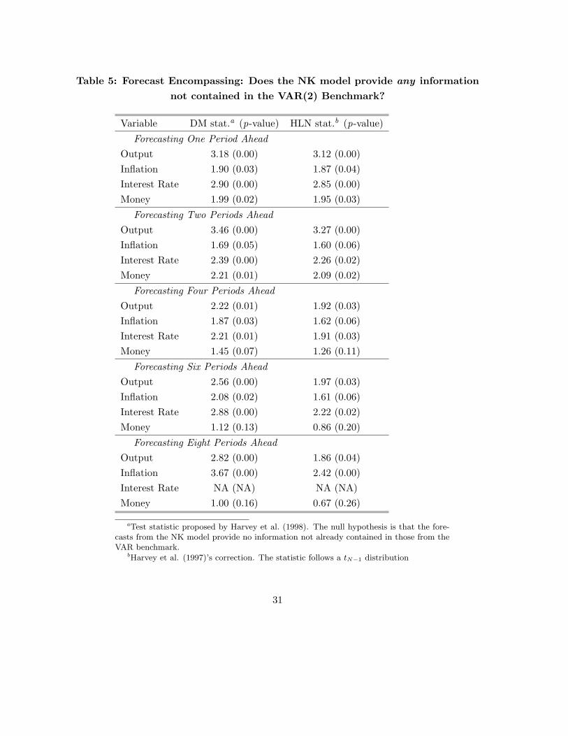
Table 5: Forecast Encompassing: Does the NK model provide any information

not contained in the VAR(2) Benchmark?

Variable DM stat.a (p-value) HLN stat.b (p-value)

Forecasting One Period Ahead

Output 3.18 (0.00) 3.12 (0.00)

Inflation 1.90 (0.03) 1.87 (0.04)

Interest Rate 2.90 (0.00) 2.85 (0.00)

Money 1.99 (0.02) 1.95 (0.03)

Forecasting Two Periods Ahead

Output 3.46 (0.00) 3.27 (0.00)

Inflation 1.69 (0.05) 1.60 (0.06)

Interest Rate 2.39 (0.00) 2.26 (0.02)

Money 2.21 (0.01) 2.09 (0.02)

Forecasting Four Periods Ahead

Output 2.22 (0.01) 1.92 (0.03)

Inflation 1.87 (0.03) 1.62 (0.06)

Interest Rate 2.21 (0.01) 1.91 (0.03)

Money 1.45 (0.07) 1.26 (0.11)

Forecasting Six Periods Ahead

Output 2.56 (0.00) 1.97 (0.03)

Inflation 2.08 (0.02) 1.61 (0.06)

Interest Rate 2.88 (0.00) 2.22 (0.02)

Money 1.12 (0.13) 0.86 (0.20)

Forecasting Eight Periods Ahead

Output 2.82 (0.00) 1.86 (0.04)

Inflation 3.67 (0.00) 2.42 (0.00)

Interest Rate NA (NA) NA (NA)

Money 1.00 (0.16) 0.67 (0.26)

aTest statistic proposed by Harvey et al. (1998). The null hypothesis is that the fore-casts from the NK model provide no information not already contained in those from theVAR benchmark.

bHarvey et al. (1997)’s correction. The statistic follows a tN−1 distribution

31

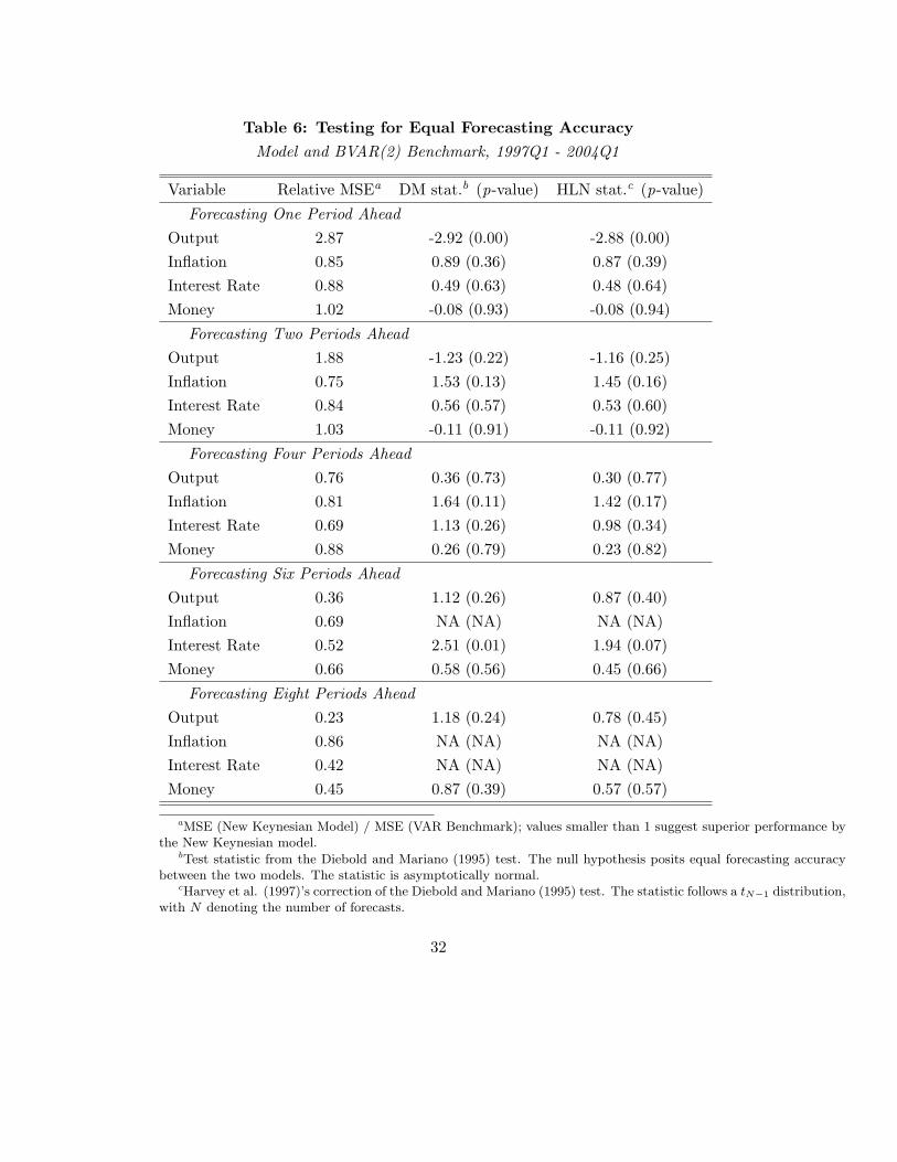
Table 6: Testing for Equal Forecasting Accuracy

Model and BVAR(2) Benchmark, 1997Q1 - 2004Q1

Variable Relative MSEa DM stat.b (p-value) HLN stat.c (p-value)

Forecasting One Period Ahead

Output 2.87 -2.92 (0.00) -2.88 (0.00)

Inflation 0.85 0.89 (0.36) 0.87 (0.39)

Interest Rate 0.88 0.49 (0.63) 0.48 (0.64)

Money 1.02 -0.08 (0.93) -0.08 (0.94)

Forecasting Two Periods Ahead

Output 1.88 -1.23 (0.22) -1.16 (0.25)

Inflation 0.75 1.53 (0.13) 1.45 (0.16)

Interest Rate 0.84 0.56 (0.57) 0.53 (0.60)

Money 1.03 -0.11 (0.91) -0.11 (0.92)

Forecasting Four Periods Ahead

Output 0.76 0.36 (0.73) 0.30 (0.77)

Inflation 0.81 1.64 (0.11) 1.42 (0.17)

Interest Rate 0.69 1.13 (0.26) 0.98 (0.34)

Money 0.88 0.26 (0.79) 0.23 (0.82)

Forecasting Six Periods Ahead

Output 0.36 1.12 (0.26) 0.87 (0.40)

Inflation 0.69 NA (NA) NA (NA)

Interest Rate 0.52 2.51 (0.01) 1.94 (0.07)

Money 0.66 0.58 (0.56) 0.45 (0.66)

Forecasting Eight Periods Ahead

Output 0.23 1.18 (0.24) 0.78 (0.45)

Inflation 0.86 NA (NA) NA (NA)

Interest Rate 0.42 NA (NA) NA (NA)

Money 0.45 0.87 (0.39) 0.57 (0.57)

aMSE (New Keynesian Model) / MSE (VAR Benchmark); values smaller than 1 suggest superior performance bythe New Keynesian model.

bTest statistic from the Diebold and Mariano (1995) test. The null hypothesis posits equal forecasting accuracybetween the two models. The statistic is asymptotically normal.

cHarvey et al. (1997)’s correction of the Diebold and Mariano (1995) test. The statistic follows a tN−1 distribution,with N denoting the number of forecasts.

32

Table 7: Testing for Equal Density Forecasting Accuracy

Model and VAR(2) Benchmark, 1997Q1 - 2004Q1, one-step-ahead density forecasts

Test statistica Significance

0.96 0.34

aTest statistic from the Amisano and Giacomini (forthcoming) test. The null hypothesis is that of equal log densityscores. The test statistic is asympotically normal

33

Figure 1: A Monetary Policy Tightening

(Shock occurs at t = 5)

0 5 10 15−0.007

−0.006

−0.005

−0.004

−0.003

−0.002

−0.001

0

Quarters

Aggregate Output

Devia

tion

from

s.s.

0 5 10 15

8.1

8.15

8.2

8.25

Quarters

Nominal Interest Rate

Net,

Annu

alize

d Ra

te (%

)

0 5 10 15 1.5

2

2.5

3

3.5

4

4.5

Quarters

Inflation

Net,

Annu

alize

d Ra

te (%

)

0 5 10 15 −1

0

1

2

3

4

5

Quarters

Money GrowthNe

t, An

nuali

zed

Rate

(%)

34

Figure 2: The Economy’s Response to a Positive Money-Demand Shock

(Shock occurs at t = 5)

0 5 10 15−0.003

−0.0025

−0.002

−0.0015

−0.001

−0.0005

0

Quarters

Aggregate Output

Devia

tion

from

s.s.

0 5 10 15 8.05

8.1

8.15

8.2

8.25

8.3

8.35

8.4

Quarters

Nominal Interest Rate

Net,

Annu

alize

d Ra

te (%

)

0 5 10 15 3.2

3.4

3.6

3.8

4

4.2

Quarters

Inflation

Net,

Annu

alize

d Ra

te (%

)

0 5 10 15 4

4.5

5

5.5

Quarters

Money GrowthNe

t, An

nuali

zed

Rate

(%)

35

Figure 3: The Economy’s Response to a Positive Technology Shock

(Shock occurs at t = 5)

0 5 10 15 0

0.001

0.002

0.003

0.004

0.005

0.006

0.007

Quarters

Aggregate Output

Devia

tion

from

s.s.

0 5 10 15 7.9

7.95

8

8.05

8.1

Quarters

Nominal Interest Rate

Net,

Annu

alize

d Ra

te (%

)

0 5 10 15 3.2

3.4

3.6

3.8

4

4.2

Quarters

Inflation

Net,

Annu

alize

d Ra

te (%

)

0 5 10 15 3.8

4

4.2

4.4

4.6

4.8

5

5.2

Quarters

Money GrowthNe

t, An

nuali

zed

Rate

(%)

36

Figure 4: The Economy’s Response to a Positive Preference Shock

(Shock occurs at t = 5)

0 5 10 15 0

0.0005

0.001

0.0015

0.002

0.0025

0.003

0.0035

Quarters

Aggregate Output

Devia

tion

from

s.s.

0 5 10 15 8

8.1

8.2

8.3

8.4

8.5

8.6

8.7

Quarters

Nominal Interest Rate

Net,

Annu

alize

d Ra

te (%

)

0 5 10 15 4

4.1

4.2

4.3

4.4

Quarters

Inflation

Net,

Annu

alize

d Ra

te (%

)

0 5 10 15 4

4.2

4.4

4.6

4.8

Quarters

Money GrowthNe

t, An

nuali

zed

Rate

(%)

37

Figure 5. Actual Data and Forecasts from the New Keynesian Model

Output

1993 1994 1995 1996 1997 1998 1999 2000 2001 2002 2003 20048.1508.1758.2008.2258.2508.2758.3008.3258.3508.375

Actual Data

One-Quarter Out

Four-Quarters Ou

Inflation

1993 1994 1995 1996 1997 1998 1999 2000 2001 2002 2003 20040.9850.9900.9951.0001.0051.0101.0151.020

Actual Data

One-Quarter Out

Four-Quarters Ou

Interest Rates

1994 1995 1996 1997 1998 1999 2000 2001 2002 20031.0050

1.0075

1.0100

1.0125

1.0150

1.0175

1.0200Actual Data

One-Quarter OutFour-Quarters Ou

Real Money Balances

1993 1994 1995 1996 1997 1998 1999 2000 2001 2002 2003 20047.527.547.567.587.607.627.647.66

Actual Data

One-Quarter Out

Four-Quarters Ou

38

Figure 6. Forecast Errors: One-Quarter Ahead

Output

Actu

al-

Pre

dic

ted

1996 1997 1998 1999 2000 2001 2002 2003-0.012

-0.008

-0.004

0.000

0.004

0.008

0.012

0.016

NK Model

VAR Benchmark

Inflation

Actu

al-

Pre

dic

ted

1996 1997 1998 1999 2000 2001 2002 2003-0.020-0.015-0.010-0.0050.0000.0050.0100.0150.0200.025

NK Model

VAR Benchmark

Interest Rates

Actu

al-

Pre

dic

ted

1996 1997 1998 1999 2000 2001 2002 2003-0.0045

-0.0036

-0.0027

-0.0018

-0.0009

0.0000

0.0009

0.0018

NK ModelVAR Benchmark

Money

Actu

al-

Pre

dic

ted

1996 1997 1998 1999 2000 2001 2002 2003-0.02

-0.01

0.00

0.01

0.02

0.03

NK Model

VAR Benchmark

39

Figure 7. Forecast Errors: Four Quarters Ahead

Output

Actu

al-

Pre

dic

ted

1996 1997 1998 1999 2000 2001 2002 2003-0.05-0.04-0.03-0.02-0.010.000.010.020.030.04

NK Model

VAR Benchmark

Inflation

Actu

al-

Pre

dic

ted

1996 1997 1998 1999 2000 2001 2002 2003-0.024

-0.016

-0.008

0.000

0.008

0.016

0.024

NK Model

VAR Benchmark

Interest Rates

Actu

al-

Pre

dic

ted

1996 1997 1998 1999 2000 2001 2002 2003-0.012-0.010-0.008-0.006-0.004-0.0020.0000.0020.004

NK Model

VAR Benchmark

Money

Actu

al-

Pre

dic

ted

1996 1997 1998 1999 2000 2001 2002 2003-0.08

-0.06

-0.04

-0.02

0.00

0.02

0.04

0.06

NK Model

VAR Benchmark

40

Figure 8. Forecast Errors: Eight Quarters Ahead

Output

Actu

al-

Pre

dic

ted

1996 1997 1998 1999 2000 2001 2002 2003-0.075

-0.050

-0.025

0.000

0.025

0.050

0.075

0.100

NK Model

VAR Benchmark

Inflation

Actu

al-

Pre

dic

ted

1996 1997 1998 1999 2000 2001 2002 2003-0.024

-0.016

-0.008

0.000

0.008

0.016

NK Model

VAR Benchmark

Interest Rates

Actu

al-

Pre

dic

ted

1996 1997 1998 1999 2000 2001 2002 2003-0.0175-0.0150-0.0125-0.0100-0.0075-0.0050-0.00250.00000.00250.0050

NK ModelVAR Benchmark

Money

Actu

al-

Pre

dic

ted

1996 1997 1998 1999 2000 2001 2002 2003-0.150-0.125-0.100-0.075-0.050-0.025-0.0000.0250.050

NK Model

VAR Benchmark

41

A Solving the New Keynesian Model

A.1 The symmetric equilibrium

ztc− 1

γ

t

cγ−1

γ

t + b1/γt m

γ−1

γ

t

= λt; (A.1)

ztb1/γt m

− 1

γ

t

cγ−1

γ

t + b1/γt m

γ−1

γ

t

= λt − βEt

(λt+1

ηπt+1

); (A.2)

ζ

1 − ht= λtwt; (A.3)

βEt

[λt+1

ηλt

(rkt+1 + 1 − δ + ηψ

(kt+2

kt+1

− 1

)kt+2

kt+1

− (ηψ/2)(kt+2

kt+1

− 1)2)]

= 1 + ηψ

(kt+1

kt− 1

); (A.4)

1

Rt= βEt

[λt+1

ηλtπt+1

](A.5)

yt = kαt (Atht)1−α; (A.6)

αytkt

= qtrt; (A.7)

(1 − α)ytht

= qtwt; (A.8)

pt =θπtθ − 1

Et∑∞

k=0(βφπ−θ)kλt+kyt+kqt+k(

∏ks=1 π

θt+s)

Et∑∞

k=0(βφπ1−θ)kλt+kyt+k(

∏ks=1 π

θ−1t+s )

; (A.9)

π1−θt = (1 − φ)p1−θ

t + φπ; (A.10)

yt = ct + ηkt+1 − (1 − δ)kt − (ψ/2)(kt+1

kt− 1)2; (A.11)

µt =ηmtπtmt−1

; (A.12)

log(Rt/R) = π log(πt/π) + y log(yt/y) + µ log(µt/µ) + log(vt); (A.13)

log(At) = (1 − ρA) log(A) + ρA log(At−1) + εAt; (A.14)

log(bt) = (1 − ρb) log(b) + ρb log(bt−1) + εbt; (A.15)

log(zt) = ρz log(zt−1) + εzt; (A.16)

log(vt) = ρv log(vt−1) + εvt. (A.17)

42

A.2 Finding The Non-stochastic Steady-State

Setting all shocks to their mean, the economy converges to a steady state in which all variables

in (A.1) to (A.17) are constant. Removing the time subscripts to denote the steady-state values

of these variables, one is lead to the following system:

µ = ηπ; (A.18)

R =π

β; (A.19)

rk =η

β− 1 + δ; (A.20)

q =θ − 1

θ; (A.21)

λc =

[1 + b

(µ

µ− β

)γ−1]−1

; (A.22)

λm = λcb

(µ

µ− β

)γ

; (A.23)

k

y=

αq

rk; (A.24)

c

y= 1 − δ

(k

y

); (A.25)

whλ =q(1 − α)(λc)

(c/y); (A.26)

h =whλ

ζ + whλ; (A.27)

y = hA

(k

y

) α1−α

. (A.28)

A.3 Linearized System

The next step in the solution is to compute a first-order approximation of (A.1) to (A.17)

around the steady state. A hatted variable denotes the deviation relative to the steady-state

value of the variable. The equations are divided between Static and Dynamic equations.

43

A.3.1 Static equations

Yt + (α− 1)ht = αkt + (1 − α)At; (A.29)

µt − πt = mt − ˆmt−1; (A.30)

Yt − rkt = kt − qt; (A.31)

(−1 − (γ − 1)λc)Ct = γλt + ((γ − 1)λ((µ− β)/µ)m)mt

+(λ((µ− β)/µ)m)bt − γzt; (A.32)

(−β/(µ− β))Rt − (λ((γ − 1)/γ)c)Ct = λt + (λ((γ − 1)/γ)(µ− β)/µ)m) + 1/γ)mt

+((λ((µ− β)/µ)m− 1)/γ)bt − zt; (A.33)

(h/(1 − h))ht − wt = λt; (A.34)

Yt − wt − ht = −qt; (A.35)

Rt − µµt − ππt − yyt = vt; (A.36)

These equations can be rewritten compactly in matrix form as

AZt = BXt + CUt

where A, B, and C are 8x8, 8x5, and 8x4 matrices, respectively and we have Zt = (yt, Rt, rkt, Ct, πt, wt, ht, µt)′

(a vector of endogenous variables), Xt = (kt, ˆmt−1, λt, qt, mt)′ (a vector of state and co-state

variables) and Ut = (At, bt, vt, zt)′ (a vector of shock variables).

A.3.2 Dynamic equations

The dynamic equations are the following:

βπt+1 = πt −(1 − βφ)(1 − φ)

φqt; (A.37)

(ψ(β(1 − δ) − (1 + β)))kt+1 + (β(1 + rk − δ))λt+1

+βrkrkt+1 + (βψy/k)yt+1 − (βψc/k)ct+1 = −ψkt + λt; (A.38)

kkt+1 = (1 − δ)kkt + yyt − cCt; (A.39)

λt+1 − πt+1 = λt − Rt; (A.40)

mt = mt. (A.41)

44

Again, this can be rewritten in matrix form as

DXt+1 + EZt+1 = FXt +GZt +HUt

where D, E, F, G, and H are 5x5, 5x8, 5x5, 5x8, and 5x4 matrices, respectively.

Using the static and dynamic equations, we can solve the model using the methodology of

Blanchard and Kahn (1980), which leads us to the following first-order state-space solution of

the system:

st+1 = Φ1st + Φ2εt+1,

dt = Φ3st,

where the matrices Φ1, Φ2 and Φ3 are functions of the structural parameters of the model.

B Data

The model is estimated using data that spans the period 1981:3 to 2004:1. The data is taken

from Statistics Canada’s CANSIM database, for which we list the associated mnemonics. Out-

put Yt is final domestic demand [V 1992068], of quarterly frequency and in chained 1987 dollars.

We convert this series into per-capita terms using the population of age 15 and over.

The interest rate Rt is the three month treasury bill rate ([V122531]), a series of daily

frequency, for which we take a quarterly average.

Finally, the money stock Mt is M2 [B1630] which is of monthly frequency; we take a

quarterly average and convert the resulting series into real, per-capita terms by dividing it

with the GDP implicit price deflator ([D100465]) and the population age 15 and over. Output

and money data are logged before estimation.

45

Documentos de Trabajo Banco Central de Chile

Working Papers Central Bank of Chile

NÚMEROS ANTERIORES PAST ISSUES

La serie de Documentos de Trabajo en versión PDF puede obtenerse gratis en la dirección electrónica: www.bcentral.cl/esp/estpub/estudios/dtbc. Existe la posibilidad de solicitar una copia impresa con un costo de $500 si es dentro de Chile y US$12 si es para fuera de Chile. Las solicitudes se pueden hacer por fax: (56-2) 6702231 o a través de correo electrónico: bcch@bcentral.cl.

Working Papers in PDF format can be downloaded free of charge from: www.bcentral.cl/eng/stdpub/studies/workingpaper. Printed versions can be ordered individually for US$12 per copy (for orders inside Chile the charge is Ch$500.) Orders can be placed by fax: (56-2) 6702231 or e-mail: bcch@bcentral.cl. DTBC-381 An Estimated Stochastic General Equilibrium Model with Partial Dollarization: A Bayesian Approach Paul Castillo, Carlos Montoso y Vicente Tuesta

Diciembre 2006

DTBC-380 Interpreting an Affine Term Structure Model for Chile Marcelo Ochoa

Diciembre 2006

DTBC-379 Speculative Currency Attacks: Role of Inconsistent Macroeconomic Policies and Real Exchange Rate Overvaluation Alfredo Pistelli

Noviembre 2006

DTBC-378 Conditional Evaluation of Exchange Rate Predictive Ability in Long Run Regressions Pablo Pincheira

Noviembre 2006

DTBC-377 Economic Growth in Latin America: From the Disappointment of the Twentieth Century to the Challenges of the Twenty-First José de Gregorio

Noviembre 2006

DTBC-376 Shrinkage Based Tests of the Martingale Difference Hypothesis Pablo Pincheira

Noviembre 2006

DTBC-375 Real Dollarization, Financial Dollarization, and Monetary Policy Alain Ize y Eric Parrado

Octubre 2006

DTBC-374 Trade Liberalization, Price Distortions, and Resource ReallocationRoberto Álvarez y Matías Braun

Agosto 2006

DTBC-373 Openness Can be Good for Growth: The Role of Policy Complementarities Roberto Chang, Linda Kaltani y Norman Loayza

Agosto 2006

DTBC-372 Market Reforms and Efficiency Gains in Chile Raphael Bergoeing, Andrés Hernando y Andrea Repetto

Agosto 2006

DTBC-371 Sovereign Debt in the Americas: New Data and Stylized Facts Kevin Cowan, Eduardo Levy-Yeyati, Ugo Panizza y Federico Sturzenegger

Agosto 2006

DTBC-370 Identifying Fiscal Policy Shocks in Chile and Colombia Jorge E. Restrepo y Hernán Rincón

Agosto 2006

DTBC-369 Bank Ownership and Lending Behavior Alejandro Micco y Ugo Panizza

Julio 2006

DTBC-368 Inflation Targeting in Dollarized Economies Leonardo Leiderman, Rodolfo Maino y Eric Parrado

Julio 2006

DTBC-367 El Banco Central de Chile en Comparación con los Bancos Centrales del Mundo Marcelo Ochoa y Klaus Schmidt-Hebbel

Junio 2006

DTBC-366 An Alternative Measure of Core Inflation Michael Pedersen

Junio 2006