Balancing Tool Chain: Balancing and automatic control in ...

General rights Copyright and moral rights for the publications made accessible in the public portal are retained by the authors and/or other copyright owners and it is a condition of accessing publications that users recognise and abide by the legal requirements associated with these rights.

Users may download and print one copy of any publication from the public portal for the purpose of private study or research.

You may not further distribute the material or use it for any profit-making activity or commercial gain

You may freely distribute the URL identifying the publication in the public portal If you believe that this document breaches copyright please contact us providing details, and we will remove access to the work immediately and investigate your claim.

Downloaded from orbit.dtu.dk on: Feb 19, 2022

Balancing Tool Chain: Balancing and automatic control in North Sea Countries in 2020,2030 and 2050

Kanellas, Polyneikis; Das, Kaushik; Gea-Bermudez, Juan; Sørensen, Poul

Publication date:2020

Document VersionPublisher's PDF, also known as Version of record

Link back to DTU Orbit

Citation (APA):Kanellas, P., Das, K., Gea-Bermudez, J., & Sørensen, P. (2020). Balancing Tool Chain: Balancing andautomatic control in North Sea Countries in 2020, 2030 and 2050. DTU Wind Energy. DTU Wind Energy E Vol.0199

https://orbit.dtu.dk/en/publications/e0f8872b-1476-4894-b334-59156aeb943b

Dep

artm

ent o

f Win

d E

nerg

y E

Rep

ort 2

020

Balancing Tool Chain : Balancing and automatic control in North Sea Countries in 2020, 2030 and 2050

NSON-DK

Deliverable 3.2

Polyneikis Kanellas, DTU Wind Energy

Kaushik Das, DTU Wind Energy

Juan Gea-Bermúdez, DTU Management

Poul Sørensen, DTU Wind Energy

DTU Wind Energy E-0199

Mar 2020

Authors: Polyneikis Kanellas1, Kaushik Das1, Juan Gea-Bermúdez2 and Poul Sørensen1

Title: Balancing Tool Chain : Balancing and automatic control in North Sea Countries in 2020, 2030 and 2050

Department: 1DTU Wind Energy. 2DTU Management

DTU Wind Energy E-0199

Mar 2020

Summary:

This report analyses a study in the balancing operation of the power system of North Sea countries with focus on the Danish power system and its regions DK1 and DK2. The study covers all the steps of the operation from the Day Ahead Market to the Real Time balancing of generation and demand. For that reason, a balancing tool chain has been developed.

The report analyses a) the value of offshore grid on balancing of forecast errors, b) the impact of forecast errors on manual and automatic reserves and c) the quality of electrical frequency in the near future considering high VRE penetration.

The simulation results clearly shows that the offshore grid scenario has very similar impact on balancing of reserves to project based scenario. Since offshore grid scenario provides additional values like increased security and flexibility as well as larger integration of North Sea countries, having similar impact on balancing as that of project based, makes offshore grid a recommendable option for future grid development. Additionally, real-time imbalance in Nordic network is much lower in case of Offshore grid scenario as compared to Project based scenario.

Day ahead market simulations for future shows higher amount of curtailment mainly pertaining to very high volume of installation of wind power. However, the volume of wind power curtailed is still low as compared to the total amount of wind power generation. This being the reason, there is no seasonal pattern in the curtailment of wind power in future scenarios.

Simulations have shown that in future, hour ahead imbalance due to wind forecast error increases in Denmark mainly in DK1. However, the hour ahead imbalance for the whole synchronous area does not increase much. Therefore, intra-hour balancing of Danish control area is largely supported from neighbouring regions. Balancing cost which is highly driven by CO2 prices in the simulation, increases substantially towards 2030. Balancing reserves in CE are largely provided by Natural Gas technologies whereas, in Nordic network, balancing reserves come from Hydro and Natural Gas. Balancing reserves in Denmark mainly come from Natural Gas. However, wind power also increases their role in balancing process in future, mainly in down regulation but also in up regulation especially if wind power is already curtailed in the day-ahead operation.

Real time imbalance seen by Nordic network increases multiple times in 2030 and 2050 scenario as compared to 2020 scenario. Additionally, the real time imbalance in Offshore grid scenario is much lower than that of Project based scenario. Nordic network is also expected to have much lower inertia available in future scenarios as compared to 2020 scenario.

The requirement for automatic frequency restoration reserves increases manifold in future scenarios as compared to 2020 scenario. Probabilistic dimensioning of frequency restoration reserves can be beneficial to mitigate the imbalances caused by wind power forecast error mainly in Nordic network. Even with proper dimensioning of frequency restoration reserves, frequency containment reserve for normal operation in Nordic network might be required to be increased in future 2030 and 2050 scenario with very high share of renewables in the power system.

Contract no.:

Grant no. 64018-0032 (EUDP, Danish energy Agency)

Project no.:

43277

Sponsorship: EUDP (previously ForskEL)

ISBN: 978-87-93549-67-8

Pages: 76

Tables: 17

References: 17

Technical University of Denmark Department of Wind Energy, Frederiksborgvej 399, Building 118, 4000 Roskilde Denmark www.vindenergi.dtu.dk [email protected]

Preface The work presented in this report is deliverable D3.2 of the North Sea Offshore Network – Denmark (NSON-DK) project. The report is prepared in collaboration between DTU Wind Energy and DTU Management.

The NSON-DK project is funded by grant no. 64018-0032 under the EUDP program administrated by the Danish energy Agency (previously under ForskEL). It is carried out as a collaboration between DTU Wind Energy (lead), DTU Management and Ea Energy Analyses.

Authors would acknowledge their gratitude to Matti Koivisto for his support in this work.

Contents

1 Introduction 8

2 Balancing Tool Chain 10

3 NSON-DK Scenarios 123.1 Countries in focus . . . . . . . . . . . . . . . . . . . . . . . . . . . . . . . . 123.2 Project-based and offshore grid scenarios . . . . . . . . . . . . . . . . . . . . 12

4 CorRES 164.1 Comparison among scenarios . . . . . . . . . . . . . . . . . . . . . . . . . . 164.2 Analysis of forecast errors . . . . . . . . . . . . . . . . . . . . . . . . . . . . 17

5 Day Ahead Market Model-Balmorel 205.1 Methodology . . . . . . . . . . . . . . . . . . . . . . . . . . . . . . . . . . . 205.2 Comparison among scenarios . . . . . . . . . . . . . . . . . . . . . . . . . . 20

6 Intra Hour Balancing Model- OptiBal 306.1 Methodology . . . . . . . . . . . . . . . . . . . . . . . . . . . . . . . . . . . 306.2 Comparison among scenarios . . . . . . . . . . . . . . . . . . . . . . . . . . 31

7 Area Control- Dynamic Model 437.1 Modelling . . . . . . . . . . . . . . . . . . . . . . . . . . . . . . . . . . . . . 437.2 Comparison among scenarios . . . . . . . . . . . . . . . . . . . . . . . . . . 47

8 Conclusion 57

Bibliography 59

A Mathematical model formulation of Day Ahead Market Model in Bal-morel 61A.1 Methodology . . . . . . . . . . . . . . . . . . . . . . . . . . . . . . . . . . . 61A.2 Mathematical model formulation . . . . . . . . . . . . . . . . . . . . . . . . 62

B Mathematical model formulation of Intra-hour Market Model in OptiBal 77B.1 Methodology . . . . . . . . . . . . . . . . . . . . . . . . . . . . . . . . . . . 77B.2 Mathematical Formulation . . . . . . . . . . . . . . . . . . . . . . . . . . . . 78

4

Nomenclature

AbbreviationsCHP Combined Heat and PowerDA Day AheadMILP Mixed Integer Linear Program-

mingUC Unit CommitmentV RE Variable Renewable EnergySetsg ∈ GGG Set of generation and pure storage

unitsi ∈ I Set of individual unitsy ∈ Y Set of yearss ∈ S Set of seasonst ∈ T Set of time stepsa ∈ A Set of areasc ∈ C Set of countriesr ∈ R Set of regionsar ∈ AR Areas in regionsrc ∈ RC Regions in countriesSubsetsAFRD ⊂ GGG Set of technologies providing

aFRR down regulationAFRU ⊂ GGG Set of technologies providing

aFRR up regulationBP ⊂ CHP Set of CHP Back Pressure gener-

ation unitsCHP ⊂ GD Set of CHP unitsEL ⊂ GGG Set of technologies delivering

electricity to consumersEXT ⊂ CHP Set of CHP Extraction genera-

tion units

FCRD ⊂ GGG Set of technologies providingFCR down regulation

FCRU ⊂ GGG Set of technologies providingFCR up regulation

GD ⊂ G Set of dispatchable generationunits

GI ⊂ G Set of intermittent generationunits

HEAT ⊂ GGG Set of technologies deliver-ing heat to consumers

HO ⊂ GD Set of heat only generation unitsHYD ⊂ GD Set of hydro storage with hydro

inflow generation unitsMFRD ⊂ GGG Set of technologies provid-

ing mFRR down regulationMFRU ⊂ GGG Set of technologies provid-

ing mFRR up regulationMRRD ⊂ GGG Set of technologies provid-

ing mRR down regulationMRRU ⊂ GGG Set of technologies provid-

ing mRR up regulationPO ⊂ GD Set of power only generation unitsPTOH ⊂ HO Set of power to heat genera-

tion unitsSLOW ⊂ GGG Set of technologies that do

not participate in the balancingmarket

G ⊂ GGG Set of generation unitsSTO ⊂ GGG Set of pure storage unitsParametersHSLa,s Maximum seasonal hydro reservoir

level [MWh]

5

HSLa,s Minimum seasonal hydro reservoirlevel [MWh]

AFg,a,y,s,t Availability factor of units [-]CBg Power-to-heat ratio [-]CVg Iso-fuel constant [-]Del

y,r,s,t Exogenous gross electricity con-sumption rate [MW]

Dha,y,s,t Exogenous gross heat consump-

tion rate [MW]ECg,a,y Installed energy capacity for pure

storage units [MWh]FCg,a,y Installed input fuel consumption

capacity [MW]HIa,y,s Seasonal hydro inflow [MWh]HLg Hours to load pure storage units

without losses[hours]HUg Hours to unload pure storage units

without losses [hours]MDTg Minimum down time [hours]MMTg Minimum maintenance time [days]MOg Minimum operation point of a gen-

eration, storage loading, or storageunloading unit relative to unit size[-]

MUTg Minimum on time [hours]SLs Season length [days]SOg,i Stochastic outage probability of

single units [-]TCRr,r′,y,s,t Transmission capacity rating [-]TLs,t Time step length [hours]USgen

g,a,y,s,t Unit size of input fuel capacity ofa generation unit [MW]

USstog,a,y,s,t Unit size of a storage unit [MWh]

ηhg Thermal efficiency [-]

ηelg Electric efficiency [-]ηstog Storage cycle efficiency [-]CCO2g,a,y CO2taxcost[€/MWh]

Cfomg,a,y Fixed cost [€/MW for generation

units, €/MWh for storage units]

Cfomg Fixed cost [€/MW for generation

units, €/MWh for storage units]Cfg,a,y Fuel cost [€/MWh]

Cong Online cost [€/MW]

Coperg,a,y Operational cost [€/MWh]

Coperg Operational cost [€/MWh]

Csdg Shut down cost [€/MW]

Csug Start up cost [€/MW]

Ctransg,r,r′,y Transmission cost [€/MWh]

TMF Maximum start time requirementfor mFRR [h]

TMR Maximum start time requirementfor mRR [h]

AFR Minimum ramping requirement foraFRR [-]

FCR Minimum ramping requirement forFCR [-]

MFR Minimum ramping requirement formFRR [-]

OAF Minimum time unit needs to be”on” to deliver aFRR (hours) [h]

OFC Minimum time unit needs to be”on” to deliver FCR (hours) [h]

AFRdny,r aFRR required- down regulation

in each hour [MW]AFRup

y,r aFRR required- up regulation ineach hour [MW]

FCRdny,r FCR required- down regulation in

each hour [MW]FCRup

y,r FCR required- up regulation ineach hour [MW]

MFRdny,r mFRR required- down regulation

in each hour [MW]MFRup

y,r mFRR required- up regulation ineach hour [MW]

MRRdny,r mRR required- down regulation in

each hour [MW]MRRup

y,r mRR required- up regulation ineach hour [MW]

Positive decision variablesdfg,a,y,s,t Fuel consumption rate [MW]

6

nav,ong,a,y,s,t Number of units available for gen-

eration online [-]nav,sdg,a,y,s,t Number of units available for gen-

eration shutting down [-]nav,sug,a,y,s,t Number of units available for gen-

eration starting up [-]nnav,pm,sdg,a,y,s,t Number of units not available for

generation stopping maintenance [-]

nnav,pm,sug,a,y,s,t Number of units not available for

generation starting maintenance [-]

nnav,pmg,a,y,s,t Number of units not available for

generation on maintenance [-]pelg,a,y,s,t Net delivered power [MW]phg,a,y,s,t Net delivered heat [MW]sog,a,y,s,t,i Stochastic outage of single units

[-]stolg,a,y,s,t Storage loading rate [MW]stonav,on

g,a,y,s,t Number of available units forloading pure storage online [-]

stonav,sdg,a,y,s,t Number of available units for

loading pure storage shuttingdown [-]

stonav,sug,a,y,s,t Number of available units for

loading pure storage starting up [-]afrrdng,a,y,s,t aFRR-down regulation power re-

served [MW]

afrrupg,a,y,s,t aFRR-up regulation power re-served [MW]

cCO2g,a,y CO2 tax annual cost [€/MWh]

cfomg,a,y Fixed annual cost [€/MW for gen-eration units, €/MWh for storageunits]

ctransg,a,y Transmission annual cost[€/MWh]

cucg,a,y Unit commitment related annualcost [€/MW]

cvomg,a,y Variable Operational annual cost[€/MWh]

fcrdng,a,y,s,t FCR-down regulation power re-served [MW]

fcrupg,a,y,s,t FCR-up regulation power re-served [MW]

hsla,y,s Hydro reservoir energy level[MWh]

mfrrdng,a,y,s,t mFRR-down regulation powerreserved [MW]

mfrrupg,a,y,s,t mFRR-up regulation power re-served [MW]

mrrdng,a,y,s,t mRR-down regulation power re-served [MW]

mrrupg,a,y,s,t mRR-up regulation power re-served [MW]

socg,a,y,s,t State of charge of pure storage[MWh]

7

Chapter 1

Introduction

The share of variable renewable energy (VRE) sources, like wind and solar is expected toincrease and become major energy resources towards the fossil fuel free energy system. Par-ticularly, in the North Sea a massive offshore wind penetration is expected. The increaseof the variable renewable energy sources in the grid brings new conditions to the energysystem due to the inherent variability and forecast uncertainty. Power imbalances due to un-certainty of the VRE poses major challenges for the reliability and security of power system.

In principal, the penetration of VRE is challenging the operation of traditional elec-tricity systems due to several facts. The marginal cost of VRE is normally lower thanthe conventional power plant’s one, leading to lower bids coming from the VRE genera-tors which means that generally VRE will be dispatched before most thermal power plants.Thus, thermal power plants with high fixed costs could become unprofitable and shut down,limiting systems adequacy. Additionally, with the increase of VRE share in the energymix, balancing requirements close to real time are expected to expand due the forecast er-rors challenging the security of supply. One of the major challenges involve balancing of thepower system with large share of VRE. To evaluate the impact of variability of VRE sourcesand imbalances caused by VRE forecast uncertainties, a complete chain of operations needto be modelled comprising of day-ahead market operation, intra-hour balancing operationand automatic frequency control. This report encompasses all these operations throughmodelling for all the North Sea countries for multiple scenarios of future energy systems.

The electricity system in Europe consists of three major types of markets which differ-entiate themselves on the time scale of the trading being made prior to real time delivery.First, is the Day Ahead (DA) electricity market which is the one where the majority ofthe energy is traded and is run daily. In this market, the buyers estimate the amount ofenergy they will demand for each hour of the next day and place their bid based on howmuch they are willing to pay for it. Similarly, sellers estimate the amount and price ofthe energy that they will be able to offer for every hour of the following day. Producersand consumers participate on the market and then the hourly prices are cleared and thegeneration schedule of the next day is created.

As expected, the forecasts done from both the buyers and sellers during the DA elec-tricity market are likely to be changed closer to the real time delivery and that is mainlycaused due to Day Ahead VRE forecast error. For that reason, the Intra-Hour (IH) market

8

is run an hour ahead from the real time. The scope of this market is to efficiently balancethe imbalance caused due to the DA forecast error using the updated hour-ahead forecasts.

Even the hour-ahead VRE generation forecasts diverge from the real time VRE gener-ation. The imbalances that will inevitably occur at the delivery time are handled by theautomatic reserves. The deployment of the automatic reserves is simulated from the AreaControl Model whose main purpose is to limit the frequency change following a disturbance.

This report analyses a) the value of future wind power development in North sea coun-tries (project based and offshore grid scenarios) on balancing of forecast errors, b) theimpact of forecast errors on manual and automatic reserves and c) the quality of the electri-cal frequency for prognosed energy scenarios of 2020, 2030 and 2050. This is accomplishedby creating a balancing tool chain simulating the three stages of power system operationdescribed above. The report is part of the WP3 of the NSON-DK project [1] and the scenar-ios used are the ones developed in WP2 [2]. The NSON-DK project studies the impact onthe system of VRE expansion in the short, medium, and long term, focusing on the Danishpower system.

9

Chapter 2

Balancing Tool Chain

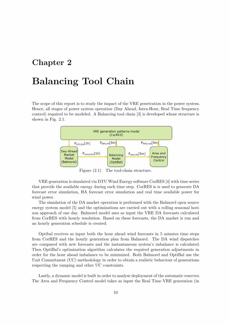
The scope of this report is to study the impact of the VRE penetration in the power system.Hence, all stages of power system operation (Day Ahead, Intra-Hour, Real Time frequencycontrol) required to be modeled. A Balancing tool chain [3] is developed whose structure isshown in Fig. 2.1.

Figure (2.1) The tool-chain structure.

VRE generation is simulated via DTU Wind Energy software CorRES [4] with time seriesthat provide the available energy during each time step. CorRES is is used to generate DAforecast error simulation, HA forecast error simulation and real time available power forwind power.

The simulation of the DA market operation is performed with the Balmorel open sourceenergy system model [5] and the optimizations are carried out with a rolling seasonal hori-zon approach of one day. Balmorel model uses as input the VRE DA forecasts calculatedfrom CorRES with hourly resolution. Based on these forecasts, the DA market is run andan hourly generation schedule is created.

Optibal receives as input both the hour ahead wind forecasts in 5 minutes time stepsfrom CorRES and the hourly generation plan from Balmorel. The DA wind dispatchesare compared with new forecasts and the instantaneous system’s imbalance is calculated.Then OptiBal’s optimization algorithm calculates the required generation adjustments inorder for the hour ahead imbalance to be minimized. Both Balmorel and OptiBal use theUnit Commitment (UC) methodology in order to obtain a realistic behaviour of generationsrespecting the ramping and other UC constraints.

Lastly, a dynamic model is built in order to analyse deployment of the automatic reserves.The Area and Frequency Control model takes as input the Real Time VRE generation (in

10

5 minutes time steps) as calculated from CorRES and the new generation plan createdfrom OptiBal (in 5 minutes time steps). With these inputs, the real time imbalance canbe determined and interpolated in 1 second time steps in order for the dynamic model tosimulate the automatic reserves deployment and the real time frequency deviations.

These tools are explained in details in next chapters.

11

Chapter 3

NSON-DK Scenarios

This chapter provides a brief overview of the scenarios used in this report. A more detaileddescription of these scenarios can be found in [2].

3.1 Countries in focusAs already mentioned, the objective of NSON-DK project is to study how the offshore windenergy development in the North Sea affects the Danish power system. Despite that Den-mark is the main focus, modelling its neighboring countries is also important since electricitysystems are heavily interconnected. The countries for which the electricity generation andtransmission development was optimized in WP2 of the NSON-DK project are : Denmark,Norway, Great Britain, Netherlands, Belgium and Germany. On the other hand, the devel-opment of other surrounding countries, such as Poland, Sweden, Finland, Estonia, Latviaand Lithuania, was not optimized but assumed. These are all the countries included inthe DA and IH market optimization performed for this report. The participating countriesare split in bidding regions and thus Denmark is divided to DK1 (West) and DK2 (East)respectively.

The Frequency Control is performed in the synchronous area level. The geographicalarea covered by ENTSO-E’s (European Network of Transmission System Operators) mem-ber TSOs is separated into five synchronous areas and two isolated systems (Cyprus andIceland). Denmark’s regions (DK1 and DK2) belong to different synchronous areas, Conti-nental Europe (CE) and Nordic respectively. Since, the scope of this report is to examinethe impact of the offshore wind energy development on the Danish power system, only coun-tries mentioned before are considered at the Area and Frequency Control model. Thus, inthis report CE consists of Belgium, Germany, Netherlands, Poland and Denmark’s regionDK1. Similarly, the Nordic synchronous area includes Norway, Sweden, Finland and DK2.

3.2 Project-based and offshore grid scenariosThe scenarios used for these studies are based on investment optimization for generationand transmission capacity for North Sea countries. A project-based scenario and an offshoregrid scenario were developed in the NSON-DK project. As shown in Fig.3.1, these scenariosare differentiated by the allowed offshore grid structure. In the investment optimization of

12

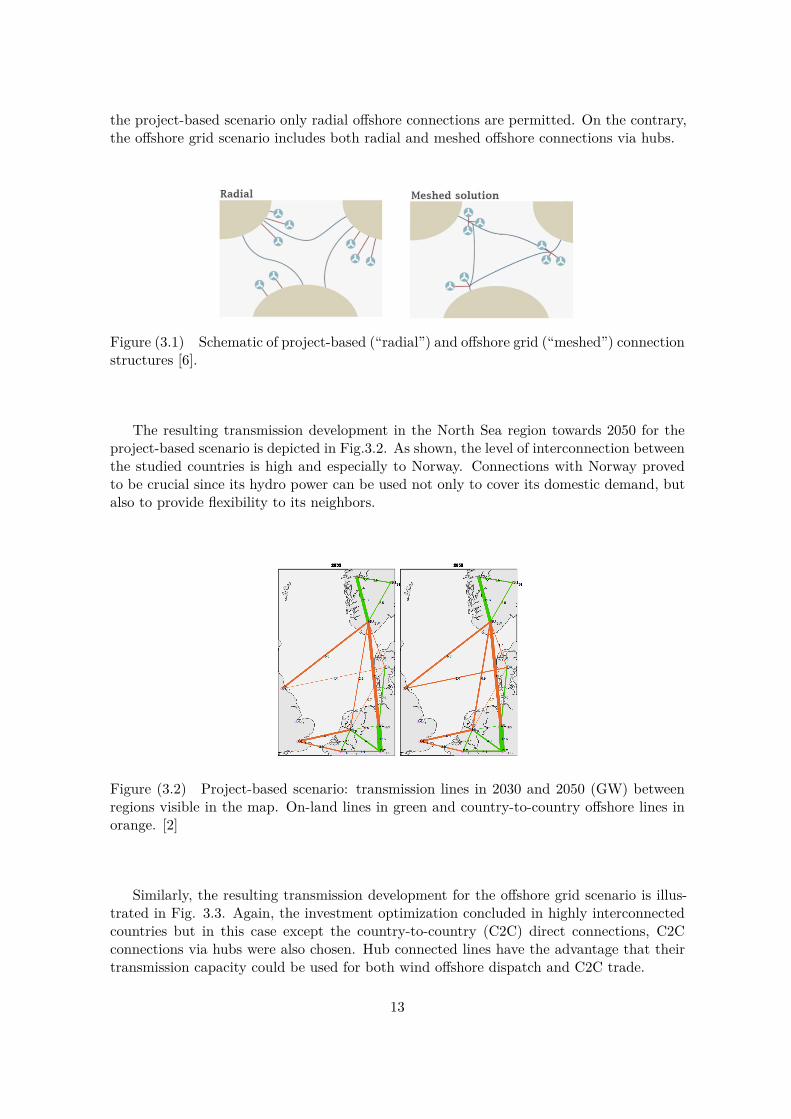
the project-based scenario only radial offshore connections are permitted. On the contrary,the offshore grid scenario includes both radial and meshed offshore connections via hubs.

Figure (3.1) Schematic of project-based (“radial”) and offshore grid (“meshed”) connectionstructures [6].

The resulting transmission development in the North Sea region towards 2050 for theproject-based scenario is depicted in Fig.3.2. As shown, the level of interconnection betweenthe studied countries is high and especially to Norway. Connections with Norway provedto be crucial since its hydro power can be used not only to cover its domestic demand, butalso to provide flexibility to its neighbors.

Figure (3.2) Project-based scenario: transmission lines in 2030 and 2050 (GW) betweenregions visible in the map. On-land lines in green and country-to-country offshore lines inorange. [2]

Similarly, the resulting transmission development for the offshore grid scenario is illus-trated in Fig. 3.3. Again, the investment optimization concluded in highly interconnectedcountries but in this case except the country-to-country (C2C) direct connections, C2Cconnections via hubs were also chosen. Hub connected lines have the advantage that theirtransmission capacity could be used for both wind offshore dispatch and C2C trade.

13

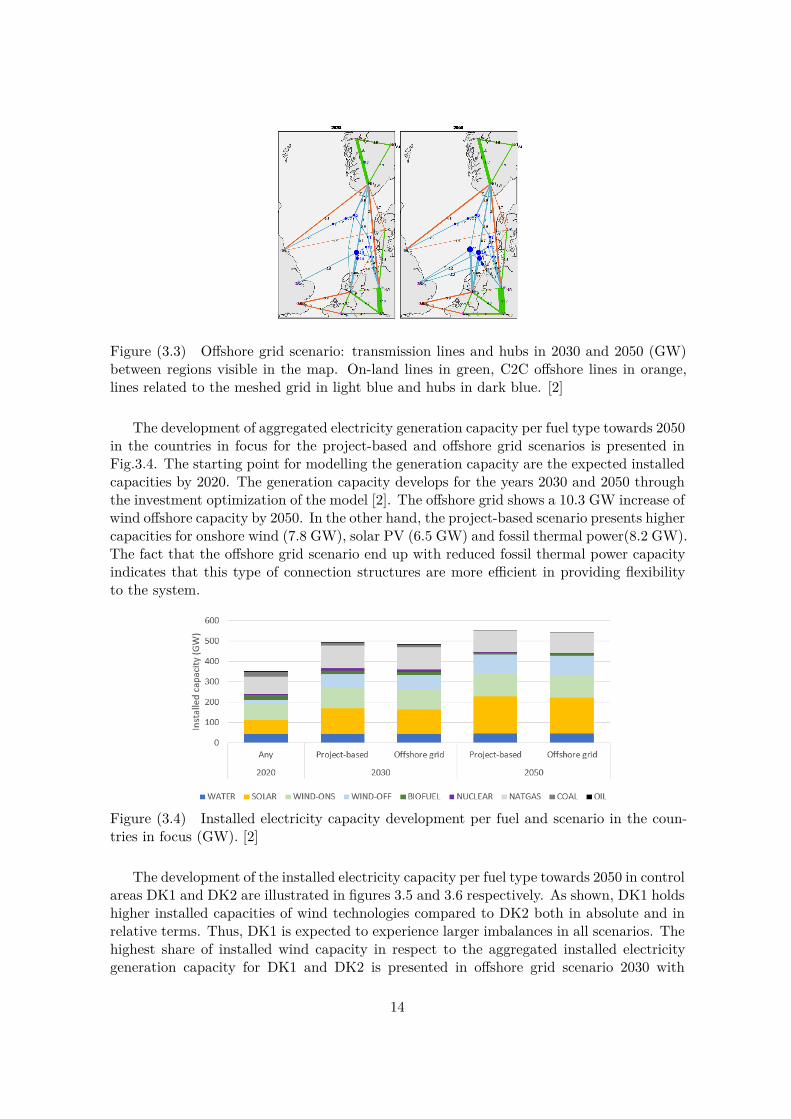
Figure (3.3) Offshore grid scenario: transmission lines and hubs in 2030 and 2050 (GW)between regions visible in the map. On-land lines in green, C2C offshore lines in orange,lines related to the meshed grid in light blue and hubs in dark blue. [2]

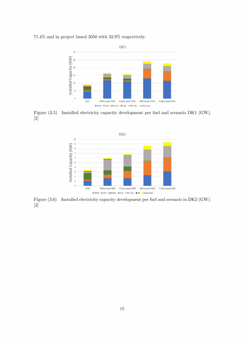
The development of aggregated electricity generation capacity per fuel type towards 2050in the countries in focus for the project-based and offshore grid scenarios is presented inFig.3.4. The starting point for modelling the generation capacity are the expected installedcapacities by 2020. The generation capacity develops for the years 2030 and 2050 throughthe investment optimization of the model [2]. The offshore grid shows a 10.3 GW increase ofwind offshore capacity by 2050. In the other hand, the project-based scenario presents highercapacities for onshore wind (7.8 GW), solar PV (6.5 GW) and fossil thermal power(8.2 GW).The fact that the offshore grid scenario end up with reduced fossil thermal power capacityindicates that this type of connection structures are more efficient in providing flexibilityto the system.

Figure (3.4) Installed electricity capacity development per fuel and scenario in the coun-tries in focus (GW). [2]

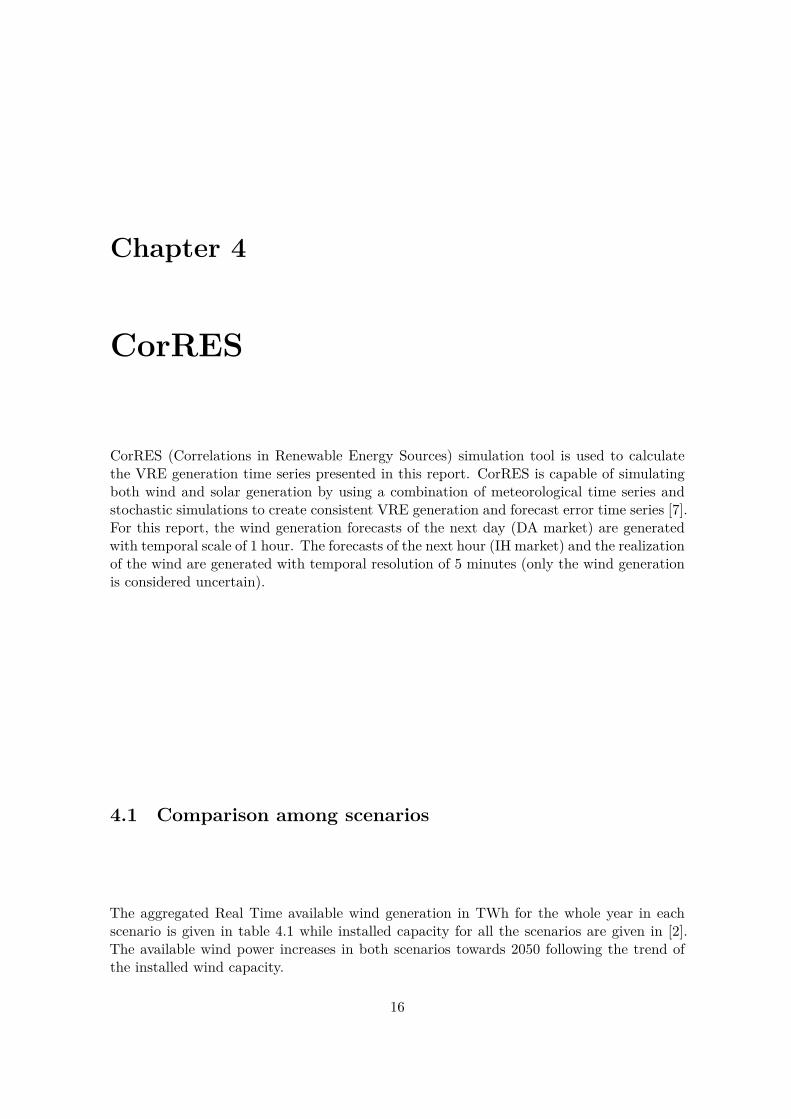
The development of the installed electricity capacity per fuel type towards 2050 in controlareas DK1 and DK2 are illustrated in figures 3.5 and 3.6 respectively. As shown, DK1 holdshigher installed capacities of wind technologies compared to DK2 both in absolute and inrelative terms. Thus, DK1 is expected to experience larger imbalances in all scenarios. Thehighest share of installed wind capacity in respect to the aggregated installed electricitygeneration capacity for DK1 and DK2 is presented in offshore grid scenario 2030 with

14

71.4% and in project based 2050 with 32.9% respectively.

Figure (3.5) Installed electricity capacity development per fuel and scenario DK1 (GW).[2]

Figure (3.6) Installed electricity capacity development per fuel and scenario in DK2 (GW).[2]

15

Chapter 4

CorRES

CorRES (Correlations in Renewable Energy Sources) simulation tool is used to calculatethe VRE generation time series presented in this report. CorRES is capable of simulatingboth wind and solar generation by using a combination of meteorological time series andstochastic simulations to create consistent VRE generation and forecast error time series [7].For this report, the wind generation forecasts of the next day (DA market) are generatedwith temporal scale of 1 hour. The forecasts of the next hour (IH market) and the realizationof the wind are generated with temporal resolution of 5 minutes (only the wind generationis considered uncertain).

4.1 Comparison among scenarios

The aggregated Real Time available wind generation in TWh for the whole year in eachscenario is given in table 4.1 while installed capacity for all the scenarios are given in [2].The available wind power increases in both scenarios towards 2050 following the trend ofthe installed wind capacity.

16

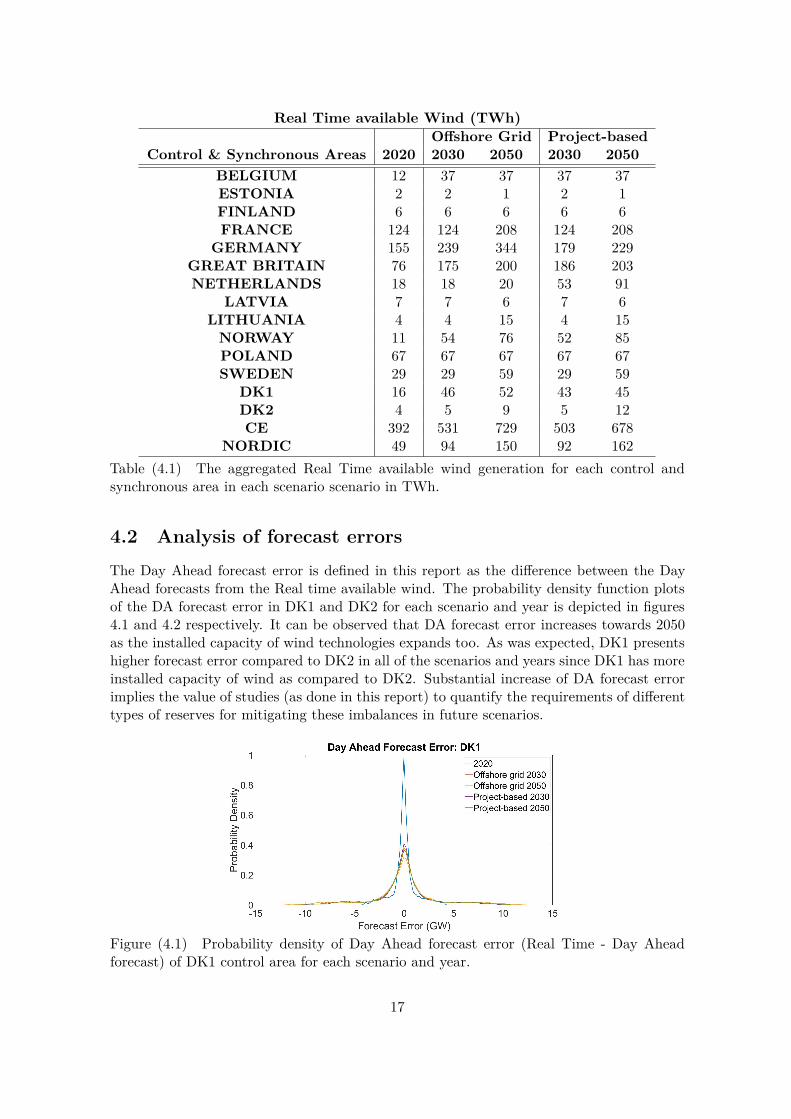
Real Time available Wind (TWh)Offshore Grid Project-based

Control & Synchronous Areas 2020 2030 2050 2030 2050BELGIUM 12 37 37 37 37ESTONIA 2 2 1 2 1FINLAND 6 6 6 6 6FRANCE 124 124 208 124 208

GERMANY 155 239 344 179 229GREAT BRITAIN 76 175 200 186 203NETHERLANDS 18 18 20 53 91

LATVIA 7 7 6 7 6LITHUANIA 4 4 15 4 15

NORWAY 11 54 76 52 85POLAND 67 67 67 67 67SWEDEN 29 29 59 29 59

DK1 16 46 52 43 45DK2 4 5 9 5 12CE 392 531 729 503 678

NORDIC 49 94 150 92 162Table (4.1) The aggregated Real Time available wind generation for each control andsynchronous area in each scenario scenario in TWh.

4.2 Analysis of forecast errorsThe Day Ahead forecast error is defined in this report as the difference between the DayAhead forecasts from the Real time available wind. The probability density function plotsof the DA forecast error in DK1 and DK2 for each scenario and year is depicted in figures4.1 and 4.2 respectively. It can be observed that DA forecast error increases towards 2050as the installed capacity of wind technologies expands too. As was expected, DK1 presentshigher forecast error compared to DK2 in all of the scenarios and years since DK1 has moreinstalled capacity of wind as compared to DK2. Substantial increase of DA forecast errorimplies the value of studies (as done in this report) to quantify the requirements of differenttypes of reserves for mitigating these imbalances in future scenarios.

Figure (4.1) Probability density of Day Ahead forecast error (Real Time - Day Aheadforecast) of DK1 control area for each scenario and year.

17

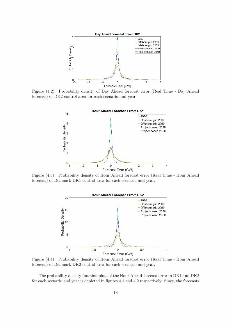
Figure (4.2) Probability density of Day Ahead forecast error (Real Time - Day Aheadforecast) of DK2 control area for each scenario and year.

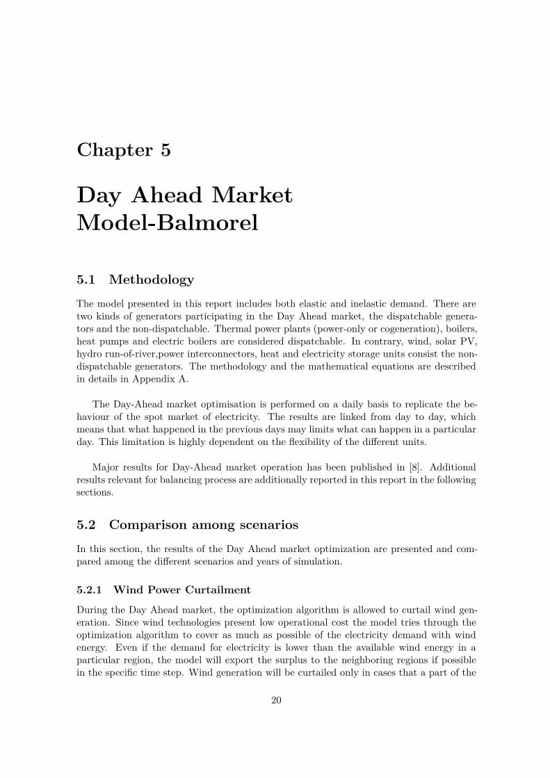
Figure (4.3) Probability density of Hour Ahead forecast error (Real Time - Hour Aheadforecast) of Denmark DK1 control area for each scenario and year.

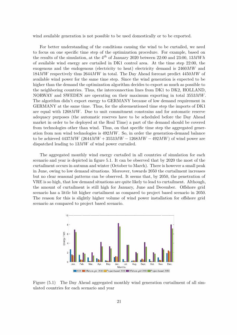
Figure (4.4) Probability density of Hour Ahead forecast error (Real Time - Hour Aheadforecast) of Denmark DK2 control area for each scenario and year.

The probability density function plots of the Hour Ahead forecast error in DK1 and DK2for each scenario and year is depicted in figures 4.1 and 4.2 respectively. Since, the forecasts

18

improve closer to the real time, forecast error reduces in Hour Ahead as compared to DayAhead forecast. Therefore, it shows the value of intra-hour balancing which in turn wouldreduce the requirements for real-time reserves. It should also be noted that Hour Aheadforecast error for 2050 scenarios for Denmark is much more than that of 2020 but almostequivalent to 2030. The reason for this is not much wind power is installed in Denmarkbetween 2030 and 2050.

These plots show the motivation for quantification of the reserve requirements for dif-ferent future scenarios as discussed in details in following chapters.

19

Chapter 5

Day Ahead MarketModel-Balmorel

5.1 MethodologyThe model presented in this report includes both elastic and inelastic demand. There aretwo kinds of generators participating in the Day Ahead market, the dispatchable genera-tors and the non-dispatchable. Thermal power plants (power-only or cogeneration), boilers,heat pumps and electric boilers are considered dispatchable. In contrary, wind, solar PV,hydro run-of-river,power interconnectors, heat and electricity storage units consist the non-dispatchable generators. The methodology and the mathematical equations are describedin details in Appendix A.

The Day-Ahead market optimisation is performed on a daily basis to replicate the be-haviour of the spot market of electricity. The results are linked from day to day, whichmeans that what happened in the previous days may limits what can happen in a particularday. This limitation is highly dependent on the flexibility of the different units.

Major results for Day-Ahead market operation has been published in [8]. Additionalresults relevant for balancing process are additionally reported in this report in the followingsections.

5.2 Comparison among scenariosIn this section, the results of the Day Ahead market optimization are presented and com-pared among the different scenarios and years of simulation.

5.2.1 Wind Power CurtailmentDuring the Day Ahead market, the optimization algorithm is allowed to curtail wind gen-eration. Since wind technologies present low operational cost the model tries through theoptimization algorithm to cover as much as possible of the electricity demand with windenergy. Even if the demand for electricity is lower than the available wind energy in aparticular region, the model will export the surplus to the neighboring regions if possiblein the specific time step. Wind generation will be curtailed only in cases that a part of the

20

wind available generation is not possible to be used domestically or to be exported.

For better understanding of the conditions causing the wind to be curtailed, we needto focus on one specific time step of the optimization procedure. For example, based onthe results of the simulation, at the 4th of January 2020 between 22:00 and 23:00, 13MWhof available wind energy are curtailed in DK1 control area. At the time step 22:00, theexogenous and the endogenous (electricity to heat) electricity demand is 2460MW and184MW respectively thus 2644MW in total. The Day Ahead forecast predict 4450MW ofavailable wind power for the same time step. Since the wind generation is expected to behigher than the demand the optimization algorithm decides to export as much as possible tothe neighboring countries. Thus, the interconnection lines from DK1 to DK2, HOLLAND,NORWAY and SWEDEN are operating on their maximum exporting in total 3553MW .The algorithm didn’t export energy to GERMANY because of low demand requirement inGERMANY at the same time. Thus, for the aforementioned time step the imports of DK1are equal with 1268MW . Due to unit commitment constrains and for automatic reserveadequacy purposes (the automatic reserves have to be scheduled before the Day Aheadmarket in order to be deployed at the Real Time) a part of the demand should be coveredfrom technologies other than wind. Thus, on that specific time step the aggregated gener-ation from non wind technologies is 492MW . So, in order the generation-demand balanceto be achieved 4437MW (2644MW + 3553MW − 1268MW − 492MW ) of wind power aredispatched leading to 13MW of wind power curtailed.

The aggregated monthly wind energy curtailed in all countries of simulation for eachscenario and year is depicted in figure 5.1. It can be observed that by 2020 the most of thecurtailment occurs in autumn and winter (October to March). There is however a small peakin June, owing to low demand situations. Moreover, towards 2050 the curtailment increasesbut no clear seasonal patterns can be observed. It seems that, by 2050, the penetration ofVRE is so high, that low demand situations are quite likely to lead to curtailment. Although,the amount of curtailment is still high for January, June and December. Offshore gridscenario has a little bit higher curtailment as compared to project based scenario in 2050.The reason for this is slightly higher volume of wind power installation for offshore gridscenario as compared to project based scenario.

Figure (5.1) The Day Ahead aggregated monthly wind generation curtailment of all sim-ulated countries for each scenario and year

21

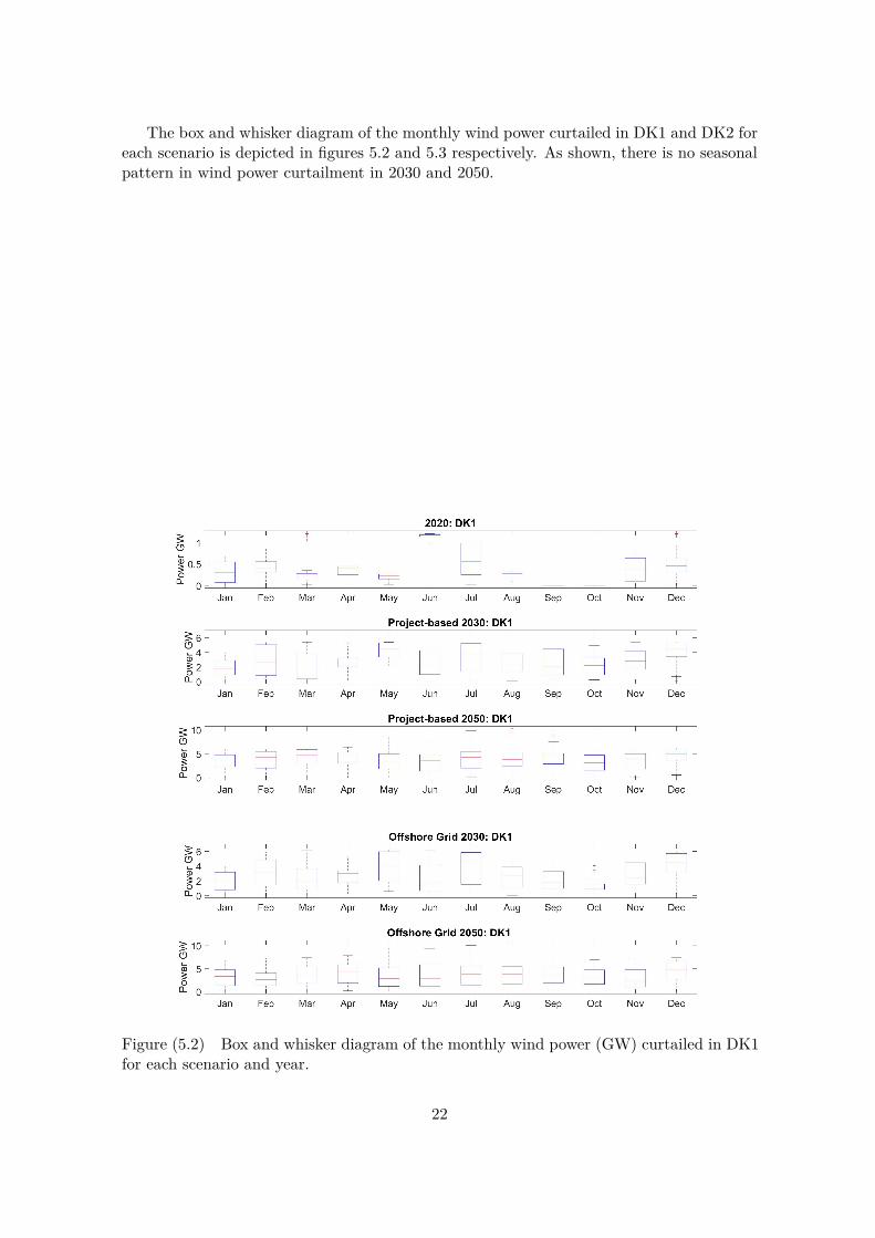
The box and whisker diagram of the monthly wind power curtailed in DK1 and DK2 foreach scenario is depicted in figures 5.2 and 5.3 respectively. As shown, there is no seasonalpattern in wind power curtailment in 2030 and 2050.

Figure (5.2) Box and whisker diagram of the monthly wind power (GW) curtailed in DK1for each scenario and year.

22

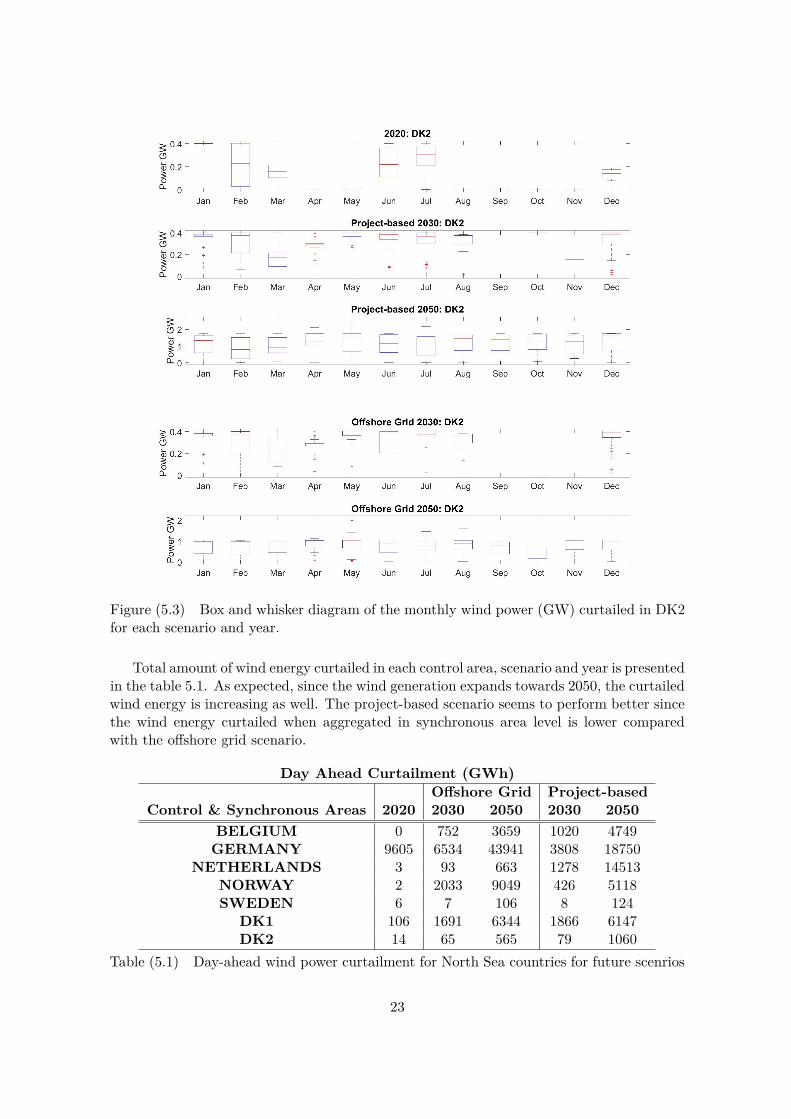
Figure (5.3) Box and whisker diagram of the monthly wind power (GW) curtailed in DK2for each scenario and year.

Total amount of wind energy curtailed in each control area, scenario and year is presentedin the table 5.1. As expected, since the wind generation expands towards 2050, the curtailedwind energy is increasing as well. The project-based scenario seems to perform better sincethe wind energy curtailed when aggregated in synchronous area level is lower comparedwith the offshore grid scenario.

Day Ahead Curtailment (GWh)Offshore Grid Project-based

Control & Synchronous Areas 2020 2030 2050 2030 2050BELGIUM 0 752 3659 1020 4749

GERMANY 9605 6534 43941 3808 18750NETHERLANDS 3 93 663 1278 14513

NORWAY 2 2033 9049 426 5118SWEDEN 6 7 106 8 124

DK1 106 1691 6344 1866 6147DK2 14 65 565 79 1060

Table (5.1) Day-ahead wind power curtailment for North Sea countries for future scenrios

23

5.2.2 Instantaneous Share of Wind Power

This section reports the results related to the instantaneous share of wind power generationin respect to the electricity demand. The cumulative distribution function of the fractionof Wind Power/Elctrecity Demand for each scenario and year for DK1 and DK2 are illus-trated in figures 5.4 and 5.5 respectively. Regarding the control area DK1, the cumulativeprobability of 100% instantaneous electrical power provided from wind in 2020 is 65% andincreases towards 2050 for both scenarios. In the other hand, in DK2, the instantaneousshare of wind power never reaches 100% in 2020 but increases towards 2050 for both scenar-ios as well. This shows that Danish power systems are major exporter of energy, but alsoit has a relevance for balancing mechanism. With no or very low amount of conventionalgenerators operating in the system, balancing responsibilities has to fall on wind powerplants and fast startup generators.

Figure (5.4) Cumulative distribution of the instantaneous share of wind power generationin respect to demand for each scenario and year in DK1.

Figure (5.5) Cumulative distribution of the instantaneous share of wind power generationin respect to demand for each scenario and year in DK2.

Next, the box and whisker diagram of the instantaneous share of the wind power inrespect to the demand for electric power, desegregated monthly, is presented for DK1 andDK2 in figures 5.6 and 5.7 respectively. Based on these results, no seasonal patterns can beobserved in the instantaneous share of wind power. The last conclusion can be explainedfrom the fact that it is common during the months with high wind penetration, the demandfor electricity to be also higher.

24

Figure (5.6) Box and whisker diagram of the monthly instantaneous share of wind powergeneration in respect to demand for DK1.

25

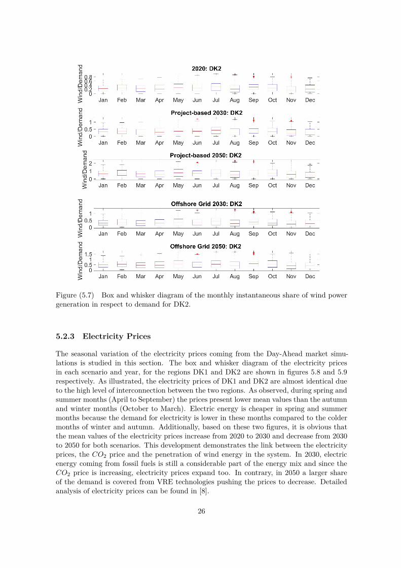
Figure (5.7) Box and whisker diagram of the monthly instantaneous share of wind powergeneration in respect to demand for DK2.

5.2.3 Electricity Prices

The seasonal variation of the electricity prices coming from the Day-Ahead market simu-lations is studied in this section. The box and whisker diagram of the electricity pricesin each scenario and year, for the regions DK1 and DK2 are shown in figures 5.8 and 5.9respectively. As illustrated, the electricity prices of DK1 and DK2 are almost identical dueto the high level of interconnection between the two regions. As observed, during spring andsummer months (April to September) the prices present lower mean values than the autumnand winter months (October to March). Electric energy is cheaper in spring and summermonths because the demand for electricity is lower in these months compared to the coldermonths of winter and autumn. Additionally, based on these two figures, it is obvious thatthe mean values of the electricity prices increase from 2020 to 2030 and decrease from 2030to 2050 for both scenarios. This development demonstrates the link between the electricityprices, the CO2 price and the penetration of wind energy in the system. In 2030, electricenergy coming from fossil fuels is still a considerable part of the energy mix and since theCO2 price is increasing, electricity prices expand too. In contrary, in 2050 a larger shareof the demand is covered from VRE technologies pushing the prices to decrease. Detailedanalysis of electricity prices can be found in [8].

26

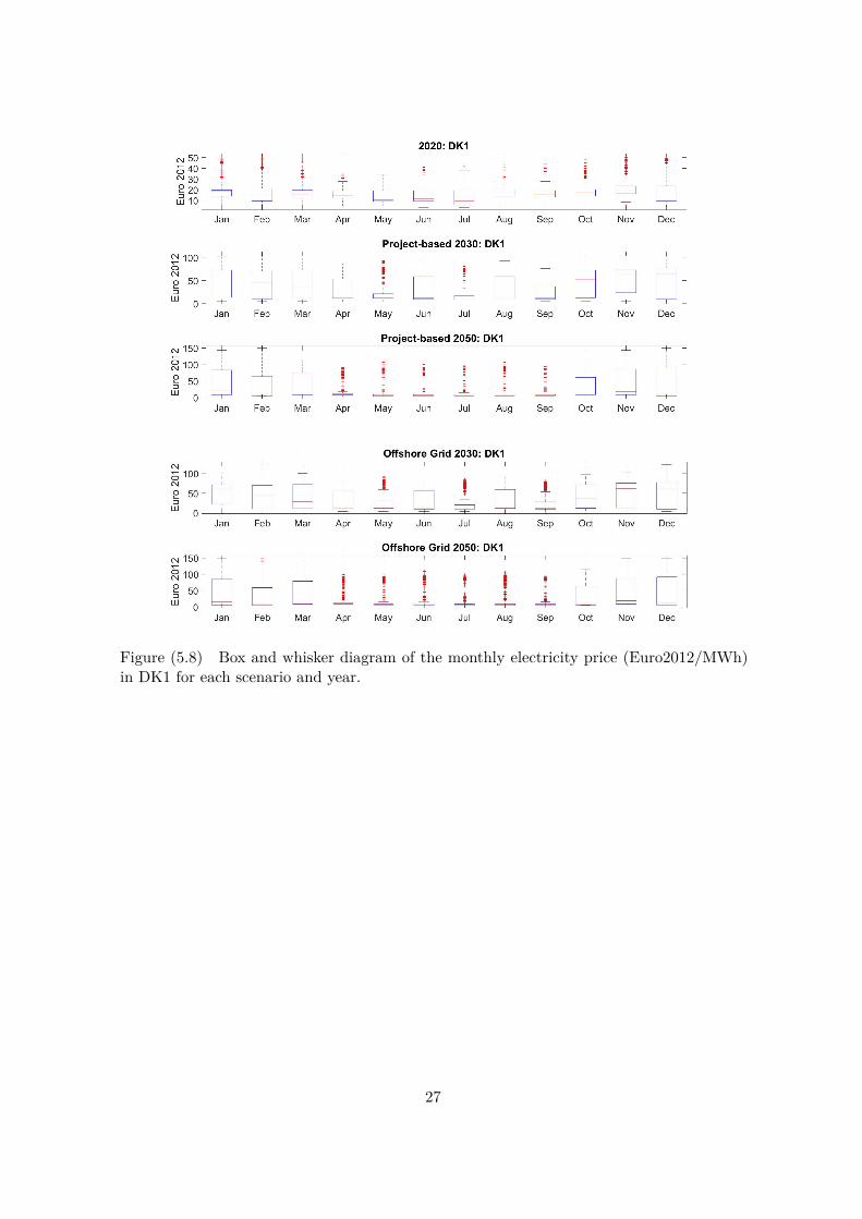
Figure (5.8) Box and whisker diagram of the monthly electricity price (Euro2012/MWh)in DK1 for each scenario and year.

27

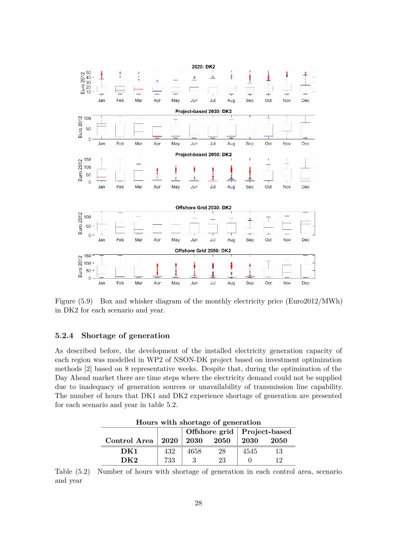
Figure (5.9) Box and whisker diagram of the monthly electricity price (Euro2012/MWh)in DK2 for each scenario and year.

5.2.4 Shortage of generation

As described before, the development of the installed electricity generation capacity ofeach region was modelled in WP2 of NSON-DK project based on investment optimizationmethods [2] based on 8 representative weeks. Despite that, during the optimization of theDay Ahead market there are time steps where the electricity demand could not be supplieddue to inadequacy of generation sources or unavailability of transmission line capability.The number of hours that DK1 and DK2 experience shortage of generation are presentedfor each scenario and year in table 5.2.

Hours with shortage of generationOffshore grid Project-based

Control Area 2020 2030 2050 2030 2050DK1 432 4658 28 4545 13DK2 733 3 23 0 12

Table (5.2) Number of hours with shortage of generation in each control area, scenarioand year

28

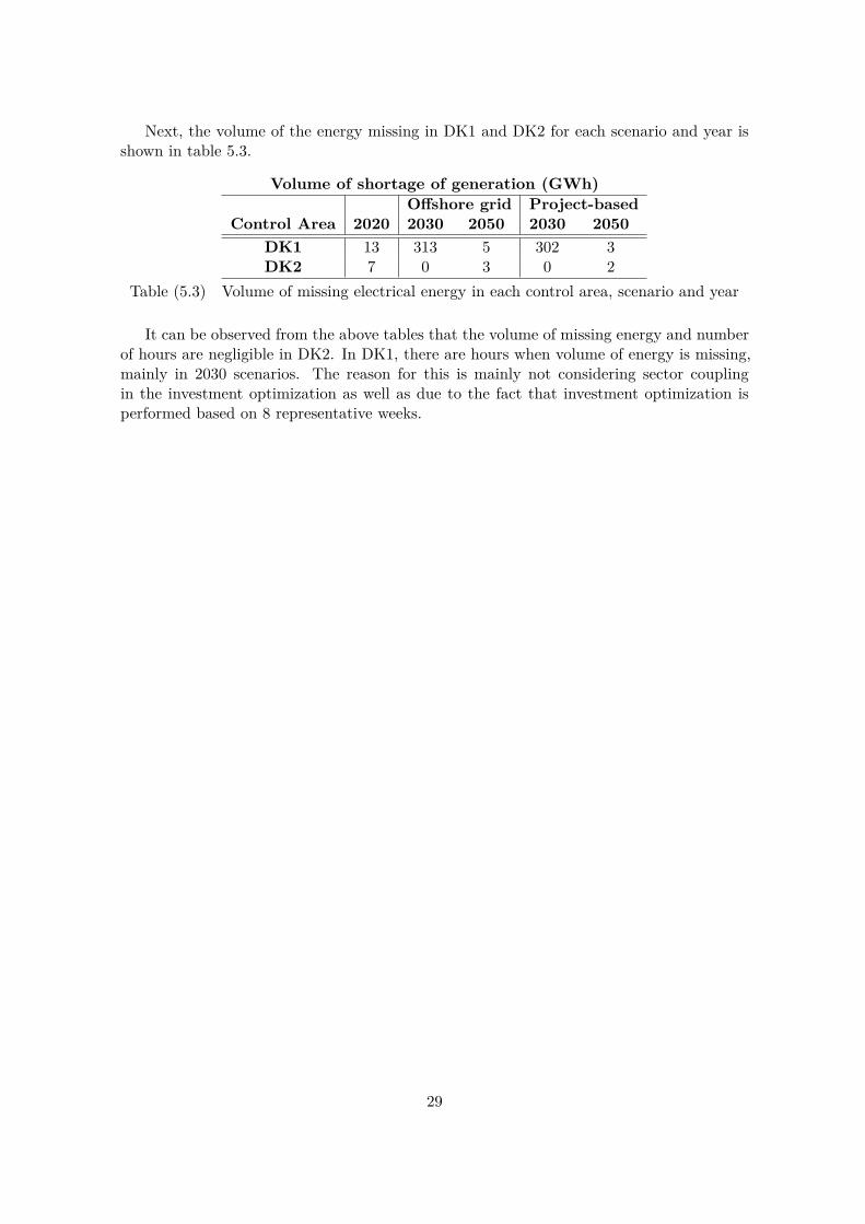
Next, the volume of the energy missing in DK1 and DK2 for each scenario and year isshown in table 5.3.

Volume of shortage of generation (GWh)Offshore grid Project-based

Control Area 2020 2030 2050 2030 2050DK1 13 313 5 302 3DK2 7 0 3 0 2

Table (5.3) Volume of missing electrical energy in each control area, scenario and year

It can be observed from the above tables that the volume of missing energy and numberof hours are negligible in DK2. In DK1, there are hours when volume of energy is missing,mainly in 2030 scenarios. The reason for this is mainly not considering sector couplingin the investment optimization as well as due to the fact that investment optimization isperformed based on 8 representative weeks.

29

Chapter 6

Intra Hour Balancing Model-OptiBal

Methodology and mathematical model of Intra-hour market and balancing is detailed inAppendix B. In this chapter, different scenarios are compared in terms of the input imbal-ance, the Intra-Hour (IH) clearing prices, the reserve activated and the number of hourswith inadequate balancing reserves. The results are mainly shown for Denmark based onthe scope of the project.

6.1 Methodology

The OptiBal model receives as input the hour ahead wind forecast simulations in temporalresolution of 5 minutes from CorRES and the hourly generation schedule from Balmorel.The main purpose of this model is to calculate the required adjustments from non VREgenerators in order to counteract the imbalance occurred due to the mismatch of the DAwind dispatches and the new wind generation forecasts.

The methodology [9] used to simulate the Intra Hour market can be split in two groups:Fixing Balancing Variables add-on and the Balancing Market optimization. The Intra Hourbalancing market optimisation is performed on a hourly basis. The results are linked fromhour to hour meaning that the results of the previous hour may limit the results in thenext hour. This limitation is highly dependent on the flexibility of the different units. Theflexibility of the units, endogenously from the model, determines whether a unit is able toparticipate in the balancing market or not.

It is important to note that OptiBal is modelled based on Danish practices for all theother countries as well. This is not true in practice today, however, this is valuable andimportant in order to model the balancing reserves required for Denmark as well as thesupport from neighboring regions during balancing operation.

30


6.2.1 Analysis of input Imbalance

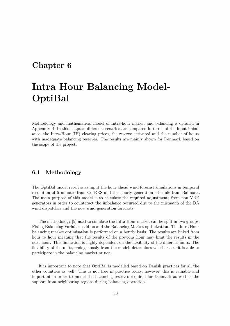
The evolution of the input imbalances towards 2050 for both project based and offshoregrid scenarios in Continental Europe and Nordic synchronous areas are shown in figure6.1 and 6.2 respectively. As shown, the volume of the imbalance follows the trend of theinstalled wind generation capacity development meaning that it is increasing towards 2050.The 5th and the 95th percentile values of the input imbalances are calculated in order toestimate the required balancing reserves. The physical significance of the 5th percentile ofthe imbalance is that equals with the reserves required to counteract 95% of the negativeimbalances occurred. Similarly, the 95th percentile gives information regarding the reservesneeded to counterbalance the 95% of the positive imbalances.

Figure (6.1) Probability density functions of Hour Ahead Imbalance (Hour Ahead forecast- Day Ahead dispatch) of Continental Europe synchronous area for each scenario and year.

From figure 6.1, it can be observed that balancing reserve requirement for CE (onlyconsidering the North Sea countries) does not change towards 2050. This is an impor-tant finding and can be attributed to the smoothening effect of large area on wind powervariability. This demonstrates that neighbouring regions can support substantially for thebalancing in each control area.

31

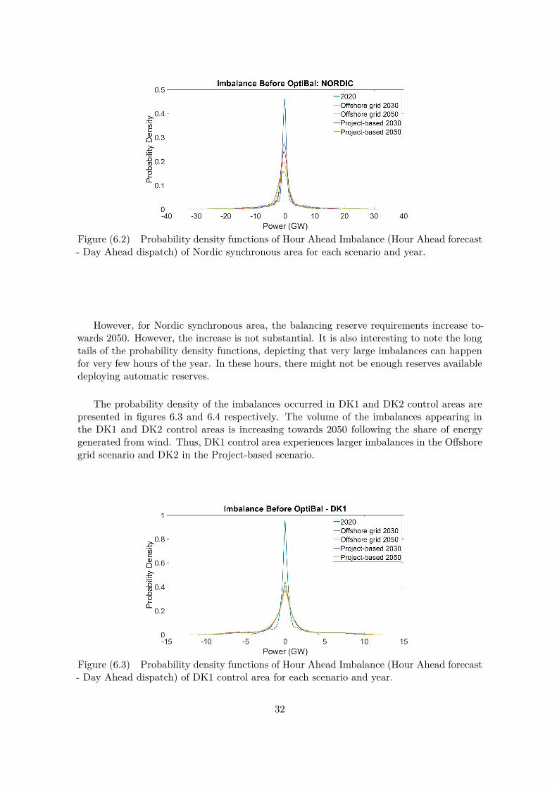
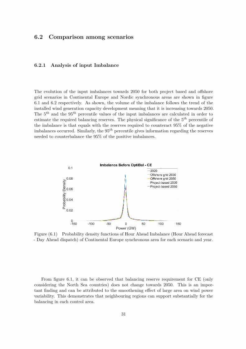
Figure (6.2) Probability density functions of Hour Ahead Imbalance (Hour Ahead forecast- Day Ahead dispatch) of Nordic synchronous area for each scenario and year.

However, for Nordic synchronous area, the balancing reserve requirements increase to-wards 2050. However, the increase is not substantial. It is also interesting to note the longtails of the probability density functions, depicting that very large imbalances can happenfor very few hours of the year. In these hours, there might not be enough reserves availabledeploying automatic reserves.

The probability density of the imbalances occurred in DK1 and DK2 control areas arepresented in figures 6.3 and 6.4 respectively. The volume of the imbalances appearing inthe DK1 and DK2 control areas is increasing towards 2050 following the share of energygenerated from wind. Thus, DK1 control area experiences larger imbalances in the Offshoregrid scenario and DK2 in the Project-based scenario.

Figure (6.3) Probability density functions of Hour Ahead Imbalance (Hour Ahead forecast- Day Ahead dispatch) of DK1 control area for each scenario and year.

32

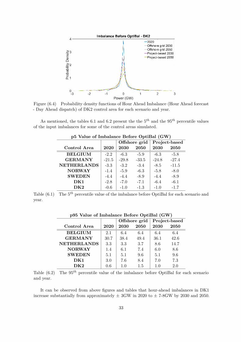
Figure (6.4) Probability density functions of Hour Ahead Imbalance (Hour Ahead forecast- Day Ahead dispatch) of DK2 control area for each scenario and year.

As mentioned, the tables 6.1 and 6.2 present the the 5th and the 95th percentile valuesof the input imbalances for some of the control areas simulated.

p5 Value of Imbalance Before OptiBal (GW)Offshore grid Project-based

Control Area 2020 2030 2050 2030 2050BELGIUM -2.2 -6.3 -5.9 -6.3 -5.8

GERMANY -21.5 -29.8 -33.5 -24.8 -27.4NETHERLANDS -3.3 -3.2 -3.4 -8.5 -11.5

NORWAY -1.4 -5.9 -6.3 -5.8 -8.0SWEDEN -4.4 -4.4 -8.9 -4.4 -8.9

DK1 -2.8 -7.0 -7.1 -6.4 -6.1DK2 -0.6 -1.0 -1.3 -1.0 -1.7

Table (6.1) The 5th percentile value of the imbalance before OptiBal for each scenario andyear.

p95 Value of Imbalance Before OptiBal (GW)Offshore grid Project-based

Control Area 2020 2030 2050 2030 2050BELGIUM 2.1 6.4 6.4 6.4 6.4

GERMANY 30.7 38.4 49.4 36.1 42.6NETHERLANDS 3.3 3.3 3.7 8.6 14.7

NORWAY 1.4 6.1 7.4 6.0 8.6SWEDEN 5.1 5.1 9.6 5.1 9.6

DK1 3.0 7.6 8.4 7.0 7.3DK2 0.6 1.0 1.5 1.0 2.0

Table (6.2) The 95th percentile value of the imbalance before OptiBal for each scenarioand year.

It can be observed from above figures and tables that hour-ahead imbalances in DK1increase substantially from approximately ± 3GW in 2020 to ± 7-8GW by 2030 and 2050.

33

While, the hour-ahead imbalances in DK2 only increase little from ± 600 MW in 2020 to± 1GW in 2030 to ± 2GW in 2050.

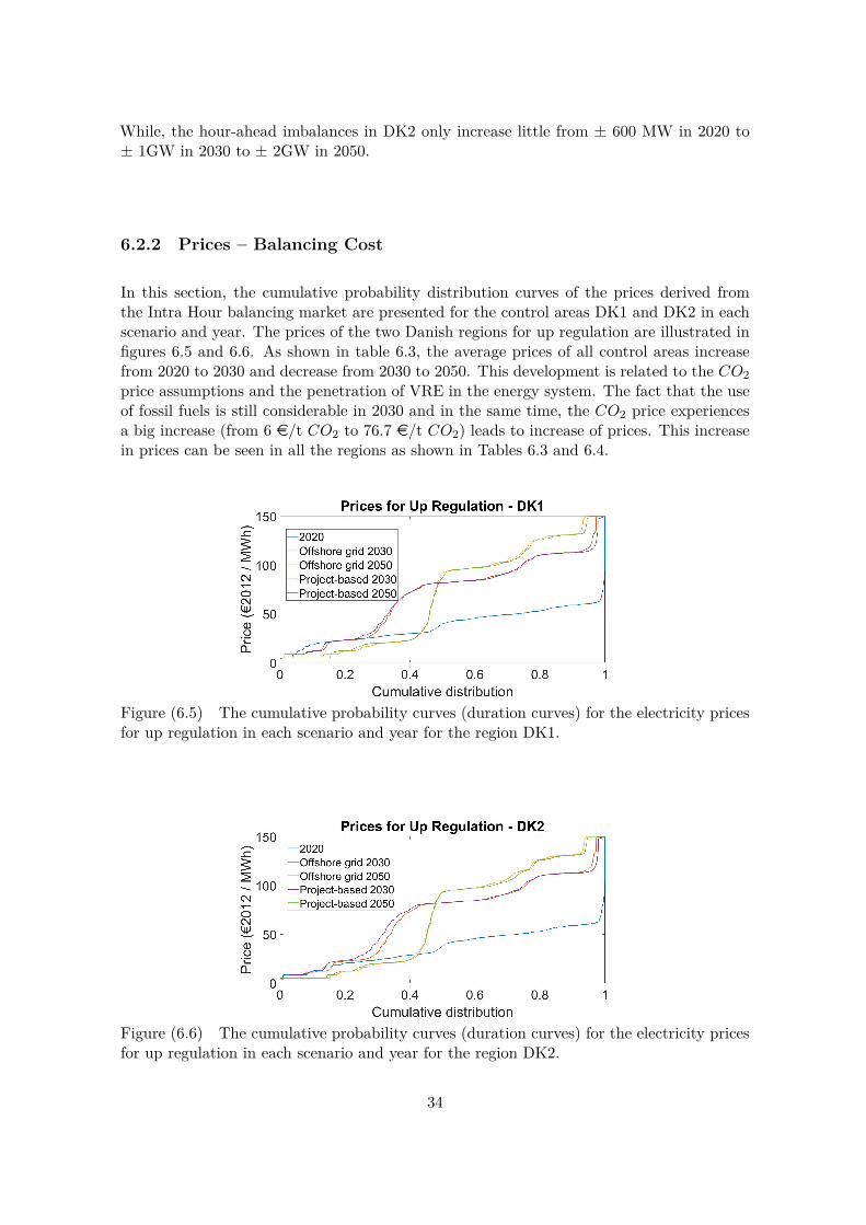
6.2.2 Prices – Balancing Cost

In this section, the cumulative probability distribution curves of the prices derived fromthe Intra Hour balancing market are presented for the control areas DK1 and DK2 in eachscenario and year. The prices of the two Danish regions for up regulation are illustrated infigures 6.5 and 6.6. As shown in table 6.3, the average prices of all control areas increasefrom 2020 to 2030 and decrease from 2030 to 2050. This development is related to the CO2

price assumptions and the penetration of VRE in the energy system. The fact that the useof fossil fuels is still considerable in 2030 and in the same time, the CO2 price experiencesa big increase (from 6 e/t CO2 to 76.7 e/t CO2) leads to increase of prices. This increasein prices can be seen in all the regions as shown in Tables 6.3 and 6.4.

Figure (6.5) The cumulative probability curves (duration curves) for the electricity pricesfor up regulation in each scenario and year for the region DK1.

Figure (6.6) The cumulative probability curves (duration curves) for the electricity pricesfor up regulation in each scenario and year for the region DK2.

34

Average Prices for Up Regulation ( e2012/MWh)Offshore grid Project-based

Control Areas 2020 2030 2050 2030 2050GERMANY 40.1 75.9 73.2 75.7 73.0

NETHERLANDS 47.5 72.2 71.5 74.2 73.6NORWAY 32.9 60.3 53.4 59.4 55.4SWEDEN 37.9 63.4 74.5 63.3 73.4

DK1 37.9 69.5 68.2 69.6 67.9DK2 36.6 69.2 68.8 70.4 68.6

Table (6.3) The average price for up regulation for each scenario and year

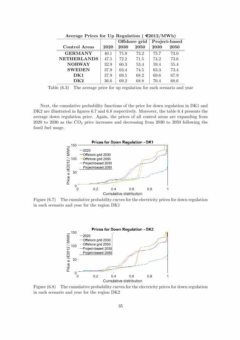
Next, the cumulative probability functions of the price for down regulation in DK1 andDK2 are illustrated in figures 6.7 and 6.8 respectively. Moreover, the table 6.4 presents theaverage down regulation price. Again, the prices of all control areas are expanding from2020 to 2030 as the CO2 price increases and decreasing from 2030 to 2050 following thefossil fuel usage.

Figure (6.7) The cumulative probability curves for the electricity prices for down regulationin each scenario and year for the region DK1

Figure (6.8) The cumulative probability curves for the electricity prices for down regulationin each scenario and year for the region DK2

35

Average Prices Down Regulation ( e2012/MWh)Offshore grid Project-based

Control Areas 2020 2030 2050 2030 2050GERMANY 21.1 46.5 40.3 47.9 41.2

NETHERLANDS 35.5 47.7 39.2 51.0 44.3NORWAY 36.2 54.2 49.5 54.7 49.8SWEDEN 29.9 47.2 47.3 47.0 47.5

DK1 24.5 46.6 41.7 47.6 43.8DK2 23.7 48.5 44.9 49.6 45.4

Table (6.4) The average price for down regulation for each scenario and year

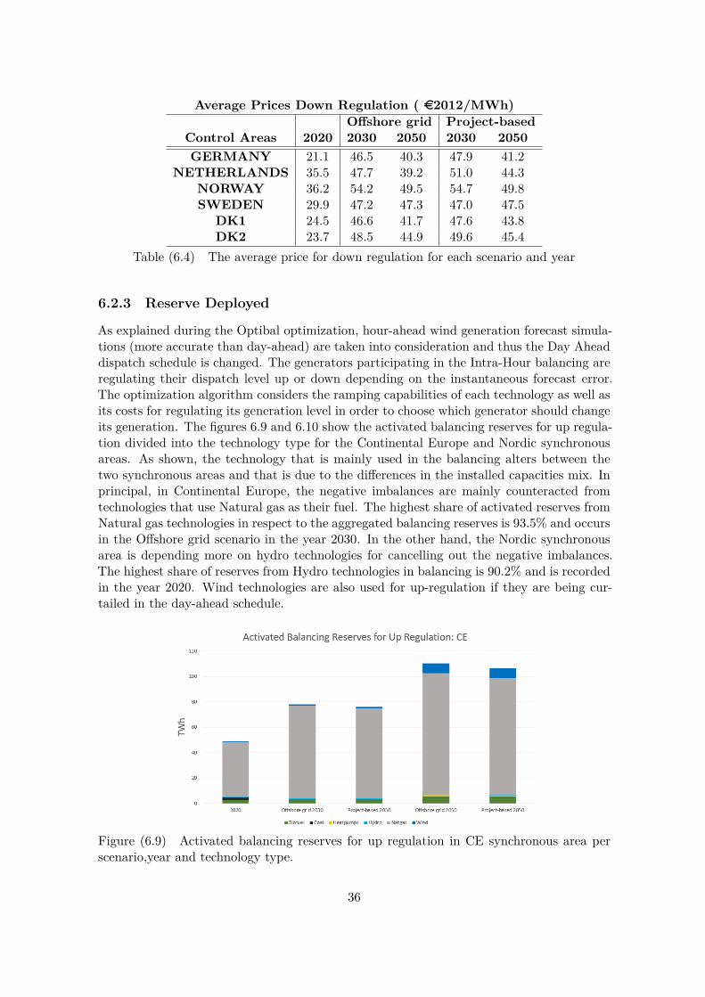
6.2.3 Reserve Deployed

As explained during the Optibal optimization, hour-ahead wind generation forecast simula-tions (more accurate than day-ahead) are taken into consideration and thus the Day Aheaddispatch schedule is changed. The generators participating in the Intra-Hour balancing areregulating their dispatch level up or down depending on the instantaneous forecast error.The optimization algorithm considers the ramping capabilities of each technology as well asits costs for regulating its generation level in order to choose which generator should changeits generation. The figures 6.9 and 6.10 show the activated balancing reserves for up regula-tion divided into the technology type for the Continental Europe and Nordic synchronousareas. As shown, the technology that is mainly used in the balancing alters between thetwo synchronous areas and that is due to the differences in the installed capacities mix. Inprincipal, in Continental Europe, the negative imbalances are mainly counteracted fromtechnologies that use Natural gas as their fuel. The highest share of activated reserves fromNatural gas technologies in respect to the aggregated balancing reserves is 93.5% and occursin the Offshore grid scenario in the year 2030. In the other hand, the Nordic synchronousarea is depending more on hydro technologies for cancelling out the negative imbalances.The highest share of reserves from Hydro technologies in balancing is 90.2% and is recordedin the year 2020. Wind technologies are also used for up-regulation if they are being cur-tailed in the day-ahead schedule.

Figure (6.9) Activated balancing reserves for up regulation in CE synchronous area perscenario,year and technology type.

36

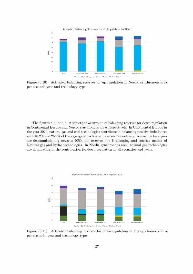
Figure (6.10) Activated balancing reserves for up regulation in Nordic synchronous areaper scenario,year and technology type.

The figures 6.11 and 6.12 depict the activation of balancing reserves for down regulationin Continental Europe and Nordic synchronous areas respectively. In Continental Europe inthe year 2020, natural gas and coal technologies contribute in balancing positive imbalanceswith 46.2% and 26.5% of the aggregated activated reserves respectively. As coal technologiesare decommissioning towards 2050, the reserves mix is changing and consists mainly ofNatural gas and hydro technologies. In Nordic synchronous area, natural gas technologiesare dominating in the contribution for down regulation in all scenarios and years.

Figure (6.11) Activated balancing reserves for down regulation in CE synchronous areaper scenario, year and technology type.

37

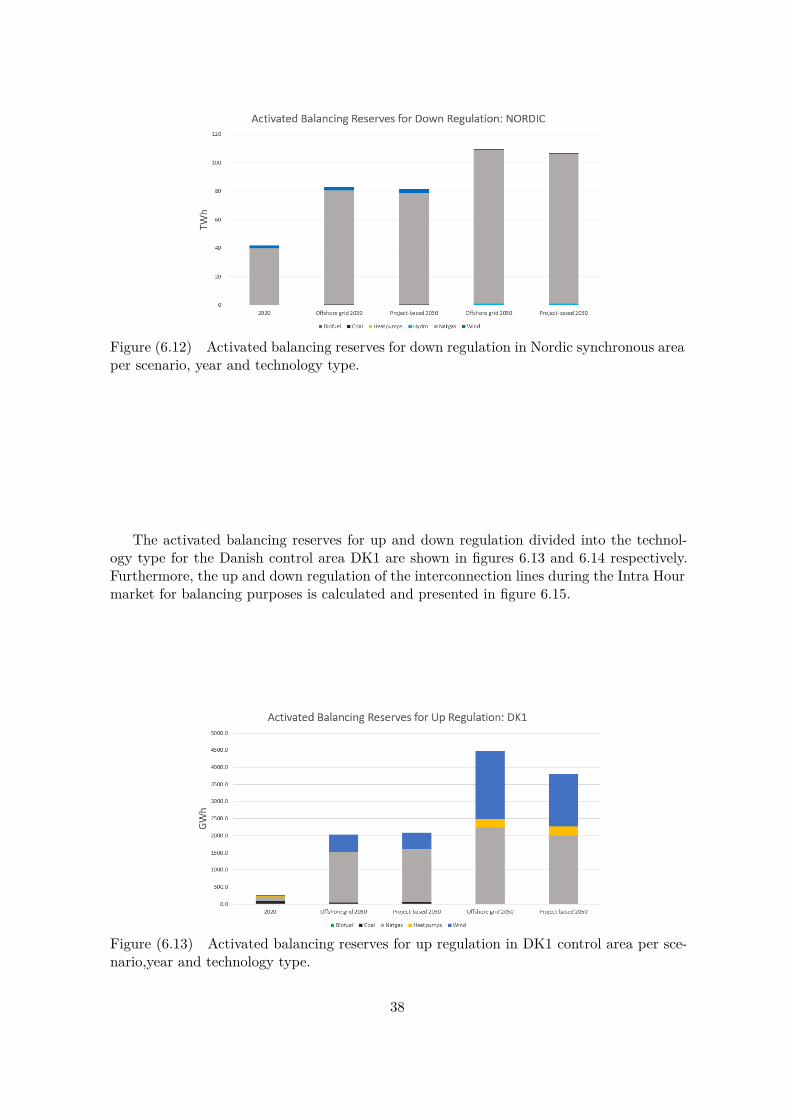
Figure (6.12) Activated balancing reserves for down regulation in Nordic synchronous areaper scenario, year and technology type.

The activated balancing reserves for up and down regulation divided into the technol-ogy type for the Danish control area DK1 are shown in figures 6.13 and 6.14 respectively.Furthermore, the up and down regulation of the interconnection lines during the Intra Hourmarket for balancing purposes is calculated and presented in figure 6.15.

Figure (6.13) Activated balancing reserves for up regulation in DK1 control area per sce-nario,year and technology type.

38

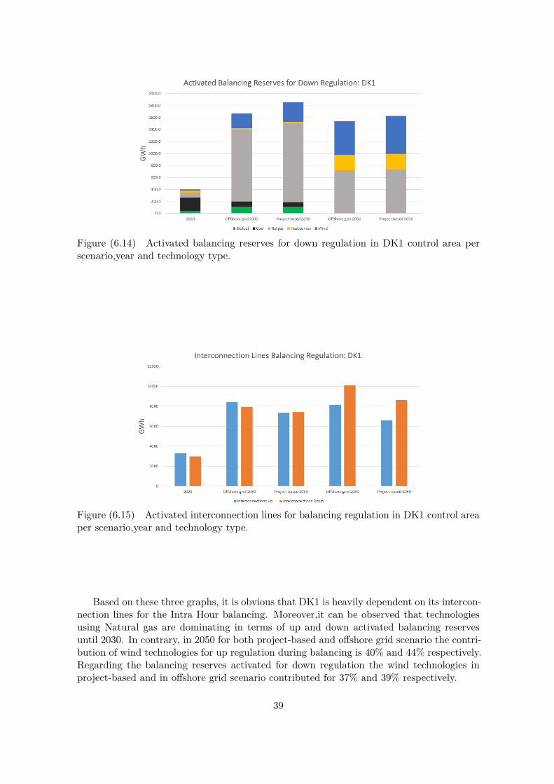
Figure (6.14) Activated balancing reserves for down regulation in DK1 control area perscenario,year and technology type.

Figure (6.15) Activated interconnection lines for balancing regulation in DK1 control areaper scenario,year and technology type.

Based on these three graphs, it is obvious that DK1 is heavily dependent on its intercon-nection lines for the Intra Hour balancing. Moreover,it can be observed that technologiesusing Natural gas are dominating in terms of up and down activated balancing reservesuntil 2030. In contrary, in 2050 for both project-based and offshore grid scenario the contri-bution of wind technologies for up regulation during balancing is 40% and 44% respectively.Regarding the balancing reserves activated for down regulation the wind technologies inproject-based and in offshore grid scenario contributed for 37% and 39% respectively.

39

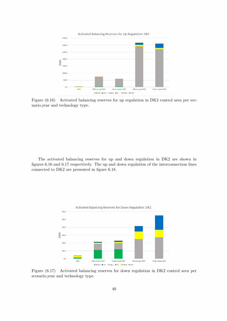
Figure (6.16) Activated balancing reserves for up regulation in DK2 control area per sce-nario,year and technology type.

The activated balancing reserves for up and down regulation in DK2 are shown infigures 6.16 and 6.17 respectively. The up and down regulation of the interconnection linesconnected to DK2 are presented in figure 6.18.

Figure (6.17) Activated balancing reserves for down regulation in DK2 control area perscenario,year and technology type.

40

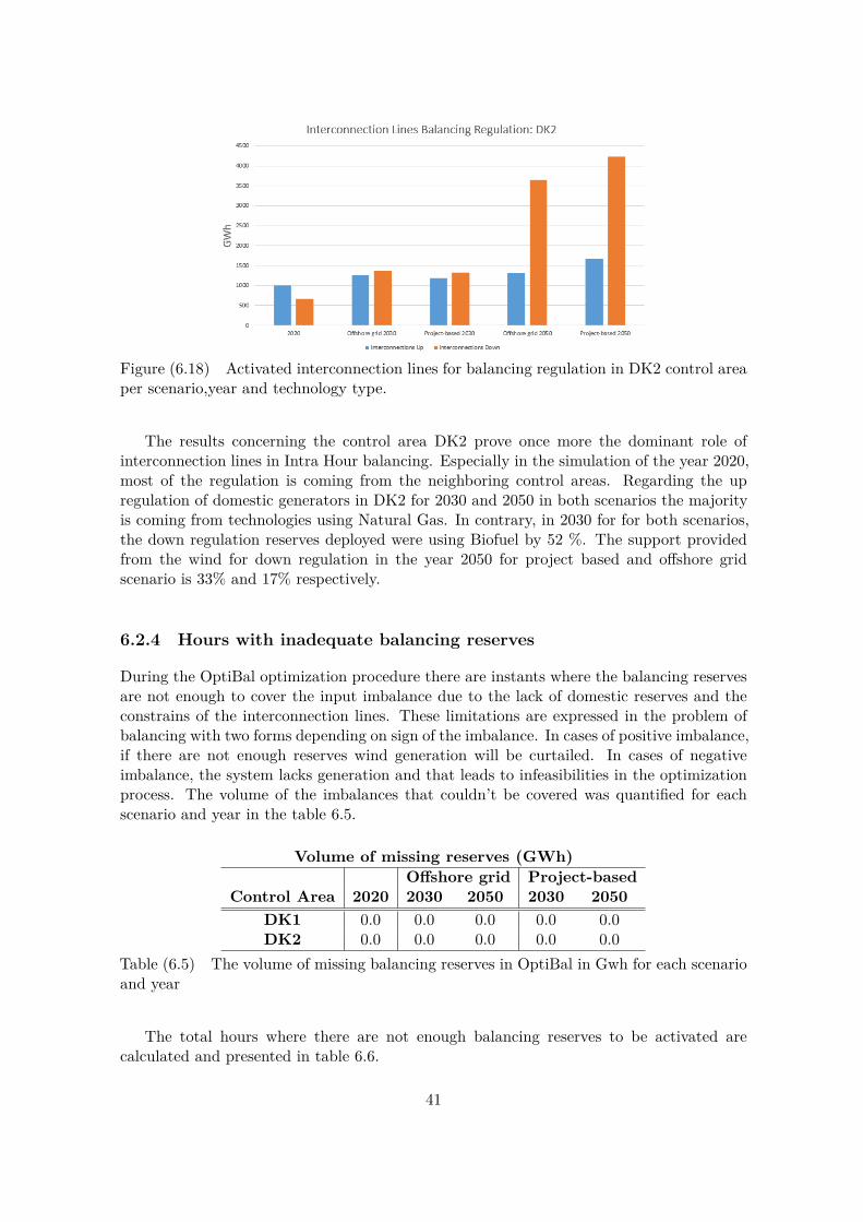
Figure (6.18) Activated interconnection lines for balancing regulation in DK2 control areaper scenario,year and technology type.

The results concerning the control area DK2 prove once more the dominant role ofinterconnection lines in Intra Hour balancing. Especially in the simulation of the year 2020,most of the regulation is coming from the neighboring control areas. Regarding the upregulation of domestic generators in DK2 for 2030 and 2050 in both scenarios the majorityis coming from technologies using Natural Gas. In contrary, in 2030 for for both scenarios,the down regulation reserves deployed were using Biofuel by 52 %. The support providedfrom the wind for down regulation in the year 2050 for project based and offshore gridscenario is 33% and 17% respectively.

6.2.4 Hours with inadequate balancing reserves

During the OptiBal optimization procedure there are instants where the balancing reservesare not enough to cover the input imbalance due to the lack of domestic reserves and theconstrains of the interconnection lines. These limitations are expressed in the problem ofbalancing with two forms depending on sign of the imbalance. In cases of positive imbalance,if there are not enough reserves wind generation will be curtailed. In cases of negativeimbalance, the system lacks generation and that leads to infeasibilities in the optimizationprocess. The volume of the imbalances that couldn’t be covered was quantified for eachscenario and year in the table 6.5.

Volume of missing reserves (GWh)Offshore grid Project-based

Control Area 2020 2030 2050 2030 2050DK1 0.0 0.0 0.0 0.0 0.0DK2 0.0 0.0 0.0 0.0 0.0

Table (6.5) The volume of missing balancing reserves in OptiBal in Gwh for each scenarioand year

The total hours where there are not enough balancing reserves to be activated arecalculated and presented in table 6.6.

41

Hours with no Balancing ReservesOffshore grid Project-based

Control & Synchronous Areas 2020 2030 2050 2030 2050DK1 0.0 0.0 0.0 0.0 0.0DK2 0.0 0.0 0.0 0.0 0.0

Table (6.6) The hours with no balancing reserves for each scenario and year.

As explained in section 5.2.4, a ”back-up” installed capacity was added in each regionin order its demand for electricity to be always covered during the Day Ahead market. InOptiBal, an ”artificial” constraint was added limiting the maximum back-up power thatcould be used in each region with the one used in DA. In case of Sweden and Norway, the”back-up” power was barely used in the DA and thus it could not be dispatched in IH. Thisis the reason for the large volume of missing reserves in these two regions.

42

Chapter 7

Area Control- Dynamic Model

In this chapter, the Area Control-Dynamic models simulating the activation of automatic re-serves and the frequency deviation for both Continental Europe and the Nordic synchronousareas are presented. In addition the aforementioned studied scenarios are compared in termsof the input imbalance, frequency deviation, FCR and FRR deployment and the instanta-neous inertia of the system. The results are only shown for a few regions for illustrativepurposes and to limit the size of this report.

7.1 Modelling

As described before, close to real time and ultimately in real time the imbalance betweenthe electricity demand and generation determines the system frequency which is crucial forsystem stability. The frequency control methodology depends on both the physical andorganisational characteristics of the particular synchronous area and thus differs amongdifferent synchronous areas of ENTSO-E [10], [11]. Although the European frameworkfor integration of the balancing markets promotes harmonization of the Balancing servicesamong the Balancing Service Providers (BSPs) each TSO may create and use specific prod-ucts. The development of these specific products is allowed when by utilizing the standardproducts alone it can be proved that a) they cannot ensure the operational security, b) theyare insufficient to maintain the system balance or c) there are balancing resources that arenot able to participate in the balancing market through standard products [12].

TSOs have the responsibility of maintaining the operational security within the definedlimits by utilizing manual and automatic reserves in mainly three balancing processes. Thebalancing products used in areas of ENTSO-E and the time scale of their deployment sincean imbalance occurs are shown in figure 7.1.

43

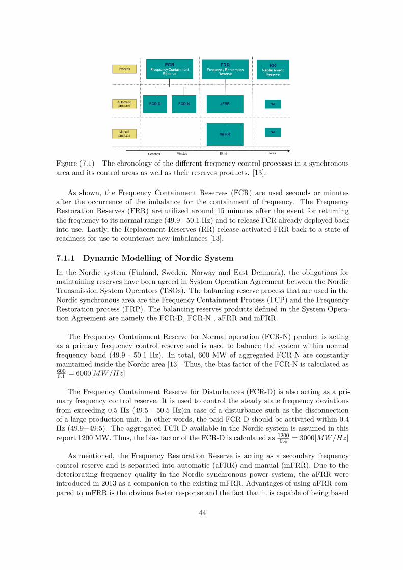
Figure (7.1) The chronology of the different frequency control processes in a synchronousarea and its control areas as well as their reserves products. [13].

As shown, the Frequency Containment Reserves (FCR) are used seconds or minutesafter the occurrence of the imbalance for the containment of frequency. The FrequencyRestoration Reserves (FRR) are utilized around 15 minutes after the event for returningthe frequency to its normal range (49.9 - 50.1 Hz) and to release FCR already deployed backinto use. Lastly, the Replacement Reserves (RR) release activated FRR back to a state ofreadiness for use to counteract new imbalances [13].

7.1.1 Dynamic Modelling of Nordic SystemIn the Nordic system (Finland, Sweden, Norway and East Denmark), the obligations formaintaining reserves have been agreed in System Operation Agreement between the NordicTransmission System Operators (TSOs). The balancing reserve process that are used in theNordic synchronous area are the Frequency Containment Process (FCP) and the FrequencyRestoration process (FRP). The balancing reserves products defined in the System Opera-tion Agreement are namely the FCR-D, FCR-N , aFRR and mFRR.

The Frequency Containment Reserve for Normal operation (FCR-N) product is actingas a primary frequency control reserve and is used to balance the system within normalfrequency band (49.9 - 50.1 Hz). In total, 600 MW of aggregated FCR-N are constantlymaintained inside the Nordic area [13]. Thus, the bias factor of the FCR-N is calculated as6000.1 = 6000[MW/Hz]

The Frequency Containment Reserve for Disturbances (FCR-D) is also acting as a pri-mary frequency control reserve. It is used to control the steady state frequency deviationsfrom exceeding 0.5 Hz (49.5 - 50.5 Hz)in case of a disturbance such as the disconnectionof a large production unit. In other words, the paid FCR-D should be activated within 0.4Hz (49.9−49.5). The aggregated FCR-D available in the Nordic system is assumed in thisreport 1200 MW. Thus, the bias factor of the FCR-D is calculated as 1200

0.4 = 3000[MW/Hz]

As mentioned, the Frequency Restoration Reserve is acting as a secondary frequencycontrol reserve and is separated into automatic (aFRR) and manual (mFRR). Due to thedeteriorating frequency quality in the Nordic synchronous power system, the aFRR wereintroduced in 2013 as a companion to the existing mFRR. Advantages of using aFRR com-pared to mFRR is the obvious faster response and the fact that it is capable of being based

44

on a merit order and taking into account the congestion in the grid.

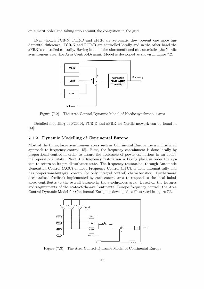
Even though FCR-N, FCR-D and aFRR are automatic they present one more fun-damental difference. FCR-N and FCR-D are controlled locally and in the other hand theaFRR is controlled centrally. Having in mind the aforementioned characteristics the Nordicsynchronous area, the Area Control-Dynamic Model is developed as shown in figure 7.2.

Figure (7.2) The Area Control-Dynamic Model of Nordic synchronous area

Detailed modelling of FCR-N, FCR-D and aFRR for Nordic network can be found in[14].

7.1.2 Dynamic Modelling of Continental EuropeMost of the times, large synchronous areas such as Continental Europe use a multi-tieredapproach to frequency control [15]. First, the frequency containment is done locally byproportional control in order to ensure the avoidance of power oscillations in an abnor-mal operational state. Next, the frequency restoration is taking place in order the sys-tem to return to its pre-disturbance state. The frequency restoration, through AutomaticGeneration Control (AGC) or Load-Frequency Control (LFC), is done automatically andhas proportional-integral control (or only integral control) characteristics. Furthermore,decentralised feedback implemented by each control area to respond to the local imbal-ance, contributes to the overall balance in the synchronous area. Based on the featuresand requirements of the state-of-the-art Continental Europe frequency control, the AreaControl-Dynamic Model for Continental Europe is developed as illustrated in figure 7.3.

Figure (7.3) The Area Control-Dynamic Model of Continental Europe

45

As shown, the model includes again primary and secondary frequency control but incontrast with the Nordic synchronous area the primary is consisted only from one reserveproduct called FCR. The deployment of FCR in Continental Europe is considered to comeonly from thermal power units which are controlled centrally. The simulation model ofFCR of Continental Europe is identical with the one presented in figure ??

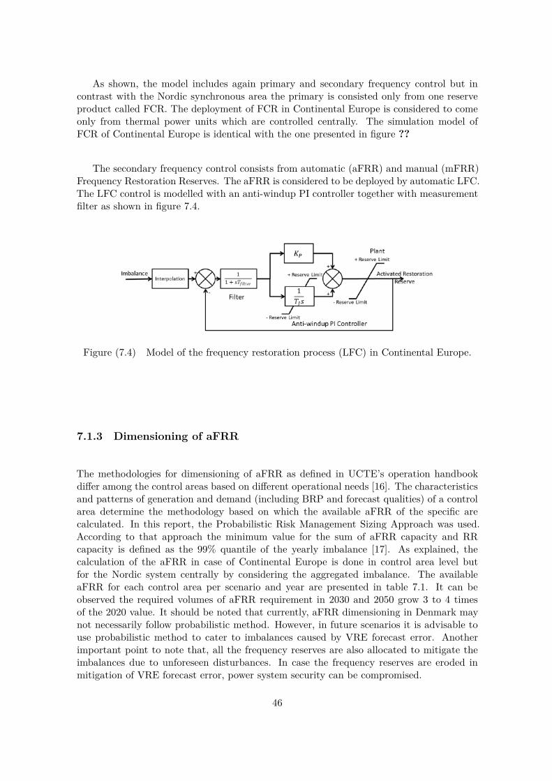
The secondary frequency control consists from automatic (aFRR) and manual (mFRR)Frequency Restoration Reserves. The aFRR is considered to be deployed by automatic LFC.The LFC control is modelled with an anti-windup PI controller together with measurementfilter as shown in figure 7.4.

Figure (7.4) Model of the frequency restoration process (LFC) in Continental Europe.

7.1.3 Dimensioning of aFRR

The methodologies for dimensioning of aFRR as defined in UCTE’s operation handbookdiffer among the control areas based on different operational needs [16]. The characteristicsand patterns of generation and demand (including BRP and forecast qualities) of a controlarea determine the methodology based on which the available aFRR of the specific arecalculated. In this report, the Probabilistic Risk Management Sizing Approach was used.According to that approach the minimum value for the sum of aFRR capacity and RRcapacity is defined as the 99% quantile of the yearly imbalance [17]. As explained, thecalculation of the aFRR in case of Continental Europe is done in control area level butfor the Nordic system centrally by considering the aggregated imbalance. The availableaFRR for each control area per scenario and year are presented in table 7.1. It can beobserved the required volumes of aFRR requirement in 2030 and 2050 grow 3 to 4 timesof the 2020 value. It should be noted that currently, aFRR dimensioning in Denmark maynot necessarily follow probabilistic method. However, in future scenarios it is advisable touse probabilistic method to cater to imbalances caused by VRE forecast error. Anotherimportant point to note that, all the frequency reserves are also allocated to mitigate theimbalances due to unforeseen disturbances. In case the frequency reserves are eroded inmitigation of VRE forecast error, power system security can be compromised.

46

aFRR available (GW)Offshore grid Project-based

Control & Synchronous Areas 2020 2030 2050 2030 2050BELGIUM 0.5 1.9 1.9 1.9 1.9


DK1 0.4 1.3 1.5 1.1 1.1Nordic 0.5 1.4 1.6 2.1 3.5

Table (7.1) The available automatic Frequency Restoration Reserves (aFRR) for eachscenario and year.


7.2.1 Analysis of Input Imbalance

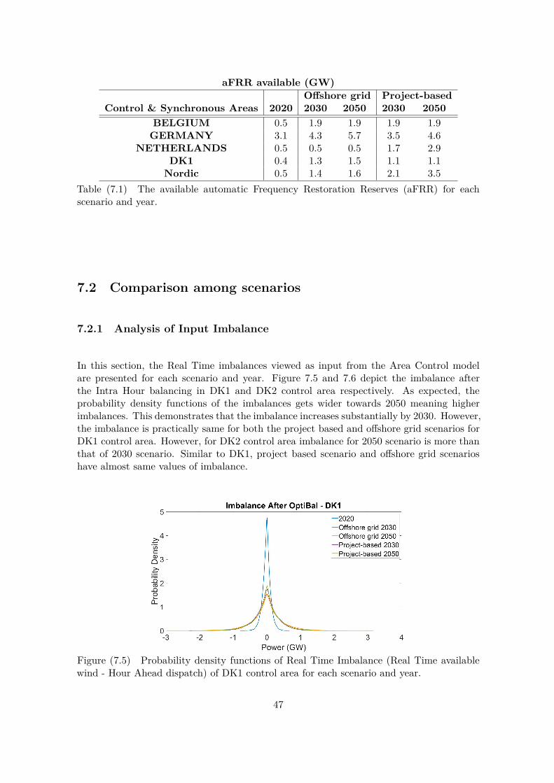
In this section, the Real Time imbalances viewed as input from the Area Control modelare presented for each scenario and year. Figure 7.5 and 7.6 depict the imbalance afterthe Intra Hour balancing in DK1 and DK2 control area respectively. As expected, theprobability density functions of the imbalances gets wider towards 2050 meaning higherimbalances. This demonstrates that the imbalance increases substantially by 2030. However,the imbalance is practically same for both the project based and offshore grid scenarios forDK1 control area. However, for DK2 control area imbalance for 2050 scenario is more thanthat of 2030 scenario. Similar to DK1, project based scenario and offshore grid scenarioshave almost same values of imbalance.

Figure (7.5) Probability density functions of Real Time Imbalance (Real Time availablewind - Hour Ahead dispatch) of DK1 control area for each scenario and year.

47

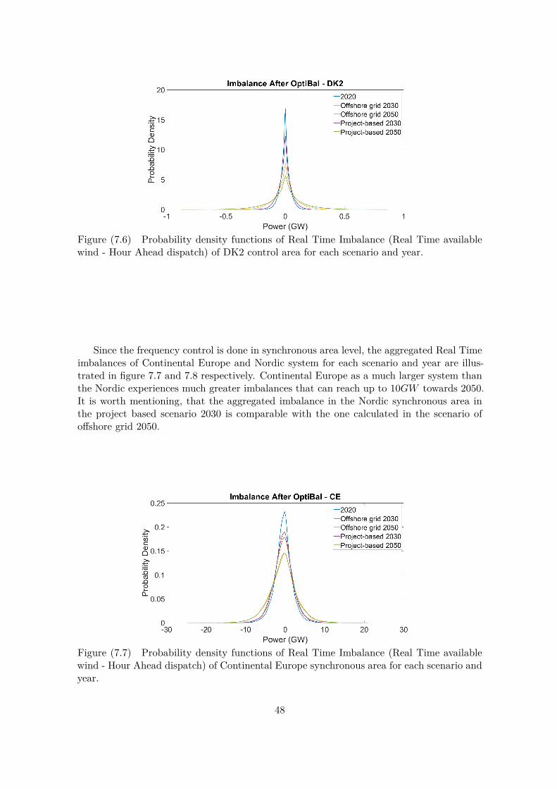
Figure (7.6) Probability density functions of Real Time Imbalance (Real Time availablewind - Hour Ahead dispatch) of DK2 control area for each scenario and year.

Since the frequency control is done in synchronous area level, the aggregated Real Timeimbalances of Continental Europe and Nordic system for each scenario and year are illus-trated in figure 7.7 and 7.8 respectively. Continental Europe as a much larger system thanthe Nordic experiences much greater imbalances that can reach up to 10GW towards 2050.It is worth mentioning, that the aggregated imbalance in the Nordic synchronous area inthe project based scenario 2030 is comparable with the one calculated in the scenario ofoffshore grid 2050.

Figure (7.7) Probability density functions of Real Time Imbalance (Real Time availablewind - Hour Ahead dispatch) of Continental Europe synchronous area for each scenario andyear.

48

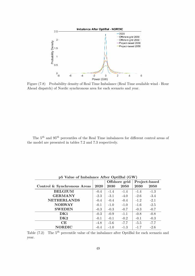
Figure (7.8) Probability density of Real Time Imbalance (Real Time available wind - HourAhead dispatch) of Nordic synchronous area for each scenario and year.

The 5th and 95th percentiles of the Real Time imbalances for different control areas ofthe model are presented in tables 7.2 and 7.3 respectively.

p5 Value of Imbalance After OptiBal (GW)Offshore grid Project-based

Control & Synchronous Areas 2020 2030 2050 2030 2050BELGIUM -0.4 -1.4 -1.4 -1.4 -1.3

GERMANY -2.3 -3.1 -4.0 -2.6 -3.4NETHERLANDS -0.4 -0.4 -0.4 -1.2 -2.1

NORWAY -0.1 -1.0 -1.0 -1.6 -2.5SWEDEN -0.3 -0.3 -0.7 -0.3 -0.7

DK1 -0.3 -0.9 -1.1 -0.8 -0.8DK2 -0.1 -0.1 -0.2 -0.1 -0.3CE -4.8 -5.6 -7.7 -5.5 -7.7

NORDIC -0.4 -1.0 -1.3 -1.7 -2.6Table (7.2) The 5th percentile value of the imbalance after OptiBal for each scenario andyear.

49

p95 Value of Imbalance After OptiBal (GW)Offshore grid Project-based

Control & Synchronous Areas 2020 2030 2050 2030 2050BELGIUM 0.4 1.3 1.3 1.3 1.3


NORWAY 0.1 0.9 1.0 1.6 2.5SWEDEN 0.3 0.3 0.6 0.3 0.6

DK1 0.2 0.9 1.0 0.7 0.8DK2 0.1 0.1 0.2 0.1 0.3CE 4.3 5.1 6.9 5 6.7

NORDIC 0.4 0.9 1.1 1.5 2.5Table (7.3) The 95th percentile value of the imbalance after OptiBal for each scenario andyear.

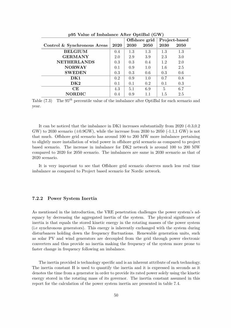
It can be noticed that the imbalance in DK1 increases substantially from 2020 (-0.3,0.2GW) to 2030 scenario (±0.9GW), while the increase from 2030 to 2050 (-1.1,1 GW) is notthat much. Offshore grid scenario has around 100 to 200 MW more imbalance pertainingto slightly more installation of wind power in offshore grid scenario as compared to projectbased scenario. The increase in imbalance for DK2 network is around 100 to 200 MWcompared to 2020 for 2050 scenario. The imbalances are same in 2030 scenario as that of2020 scenario.

It is very important to see that Offshore grid scenario observes much less real timeimbalance as compared to Project based scenario for Nordic network.

7.2.2 Power System Inertia

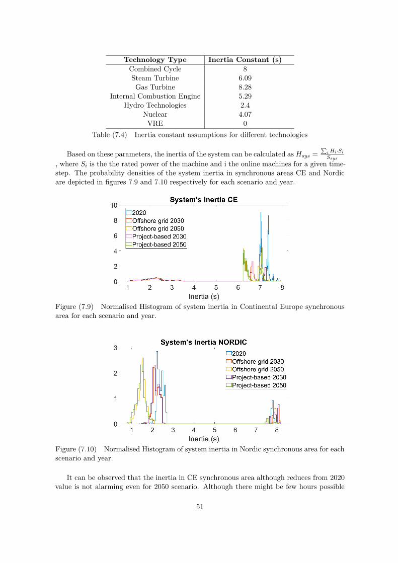
As mentioned in the introduction, the VRE penetration challenges the power system’s ad-equacy by decreasing the aggregated inertia of the system. The physical significance ofinertia is that equals the stored kinetic energy in the rotating masses of the power system(i.e synchronous generators). This energy is inherently exchanged with the system duringdisturbances holding down the frequency fluctuations. Renewable generation units, suchas solar PV and wind generators are decoupled from the grid through power electronicconverters and thus provide no inertia making the frequency of the system more prone tofaster change in frequency following an imbalance.

The inertia provided is technology specific and is an inherent attribute of each technology.The inertia constant H is used to quantify the inertia and it is expressed in seconds as itdenotes the time from a generator in order to provide its rated power solely using the kineticenergy stored in the rotating mass of its governor. The inertia constant assumed in thisreport for the calculation of the power system inertia are presented in table 7.4.

50

Technology Type Inertia Constant (s)Combined Cycle 8Steam Turbine 6.09Gas Turbine 8.28

Internal Combustion Engine 5.29Hydro Technologies 2.4

Nuclear 4.07VRE 0

Table (7.4) Inertia constant assumptions for different technologies

Based on these parameters, the inertia of the system can be calculated as Hsys =∑

i Hi·Si

Ssys

, where Si is the the rated power of the machine and i the online machines for a given time-step. The probability densities of the system inertia in synchronous areas CE and Nordicare depicted in figures 7.9 and 7.10 respectively for each scenario and year.

Figure (7.9) Normalised Histogram of system inertia in Continental Europe synchronousarea for each scenario and year.

Figure (7.10) Normalised Histogram of system inertia in Nordic synchronous area for eachscenario and year.

It can be observed that the inertia in CE synchronous area although reduces from 2020value is not alarming even for 2050 scenario. Although there might be few hours possible

51

where the inertia might go low. However, for Nordic network, the inertia is highly impactedin 2030 and 2050 scenario. Although, these inertia calculation can be pessimistic becausethe inertia of loads and other components like synchronous condensers are not taken intoaccount.

7.2.3 Frequency

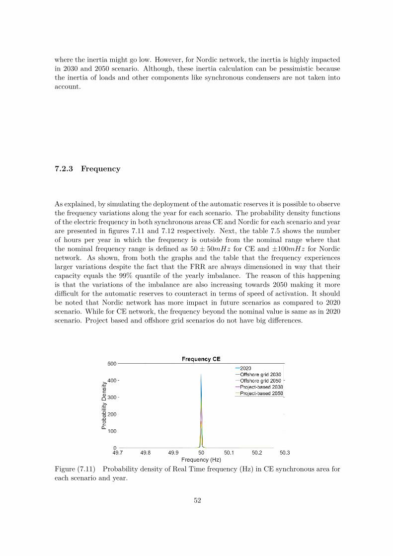
As explained, by simulating the deployment of the automatic reserves it is possible to observethe frequency variations along the year for each scenario. The probability density functionsof the electric frequency in both synchronous areas CE and Nordic for each scenario and yearare presented in figures 7.11 and 7.12 respectively. Next, the table 7.5 shows the numberof hours per year in which the frequency is outside from the nominal range where thatthe nominal frequency range is defined as 50 ± 50mHz for CE and ±100mHz for Nordicnetwork. As shown, from both the graphs and the table that the frequency experienceslarger variations despite the fact that the FRR are always dimensioned in way that theircapacity equals the 99% quantile of the yearly imbalance. The reason of this happeningis that the variations of the imbalance are also increasing towards 2050 making it moredifficult for the automatic reserves to counteract in terms of speed of activation. It shouldbe noted that Nordic network has more impact in future scenarios as compared to 2020scenario. While for CE network, the frequency beyond the nominal value is same as in 2020scenario. Project based and offshore grid scenarios do not have big differences.

Figure (7.11) Probability density of Real Time frequency (Hz) in CE synchronous area foreach scenario and year.

52

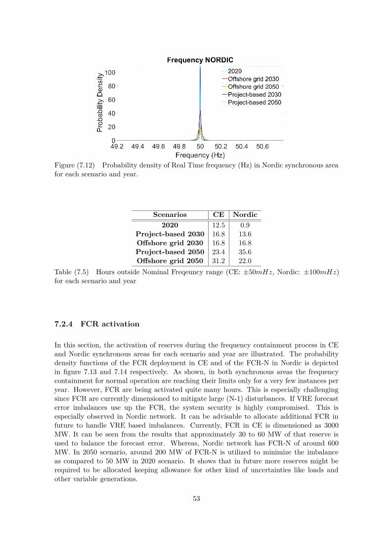
Figure (7.12) Probability density of Real Time frequency (Hz) in Nordic synchronous areafor each scenario and year.

Scenarios CE Nordic2020 12.5 0.9

Project-based 2030 16.8 13.6Offshore grid 2030 16.8 16.8Project-based 2050 23.4 35.6Offshore grid 2050 31.2 22.0

Table (7.5) Hours outside Nominal Freqeuncy range (CE: ±50mHz, Nordic: ±100mHz)for each scenario and year

7.2.4 FCR activation

In this section, the activation of reserves during the frequency containment process in CEand Nordic synchronous areas for each scenario and year are illustrated. The probabilitydensity functions of the FCR deployment in CE and of the FCR-N in Nordic is depictedin figure 7.13 and 7.14 respectively. As shown, in both synchronous areas the frequencycontainment for normal operation are reaching their limits only for a very few instances peryear. However, FCR are being activated quite many hours. This is especially challengingsince FCR are currently dimensioned to mitigate large (N-1) disturbances. If VRE forecasterror imbalances use up the FCR, the system security is highly compromised. This isespecially observed in Nordic network. It can be advisable to allocate additional FCR infuture to handle VRE based imbalances. Currently, FCR in CE is dimensioned as 3000MW. It can be seen from the results that approximately 30 to 60 MW of that reserve isused to balance the forecast error. Whereas, Nordic network has FCR-N of around 600MW. In 2050 scenario, around 200 MW of FCR-N is utilized to minimize the imbalanceas compared to 50 MW in 2020 scenario. It shows that in future more reserves might berequired to be allocated keeping allowance for other kind of uncertainties like loads andother variable generations.

53

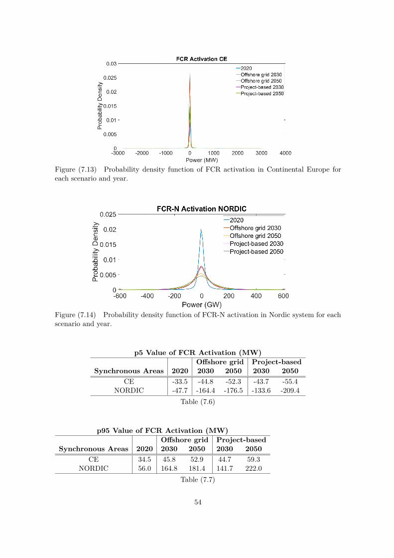
Figure (7.13) Probability density function of FCR activation in Continental Europe foreach scenario and year.

Figure (7.14) Probability density function of FCR-N activation in Nordic system for eachscenario and year.

p5 Value of FCR Activation (MW)Offshore grid Project-based

Synchronous Areas 2020 2030 2050 2030 2050CE -33.5 -44.8 -52.3 -43.7 -55.4

NORDIC -47.7 -164.4 -176.5 -133.6 -209.4Table (7.6)

p95 Value of FCR Activation (MW)Offshore grid Project-based

Synchronous Areas 2020 2030 2050 2030 2050CE 34.5 45.8 52.9 44.7 59.3

NORDIC 56.0 164.8 181.4 141.7 222.0Table (7.7)

54

Although it should be noted that there is no difference between project based andoffshore grid scenario.

7.2.5 FRR Activation

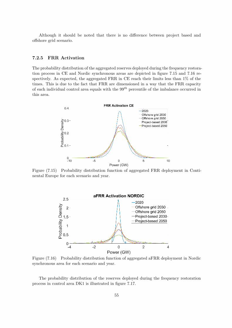
The probability distribution of the aggregated reserves deployed during the frequency restora-tion process in CE and Nordic synchronous areas are depicted in figure 7.15 and 7.16 re-spectively. As expected, the aggregated FRR in CE reach their limits less than 1% of thetimes. This is due to the fact that FRR are dimensioned in a way that the FRR capacityof each individual control area equals with the 99th percentile of the imbalance occurred inthis area.

Figure (7.15) Probability distribution function of aggregated FRR deployment in Conti-nental Europe for each scenario and year.

Figure (7.16) Probability distribution function of aggregated aFRR deployment in Nordicsynchronous area for each scenario and year.

The probability distribution of the reserves deployed during the frequency restorationprocess in control area DK1 is illustrated in figure 7.17.

55

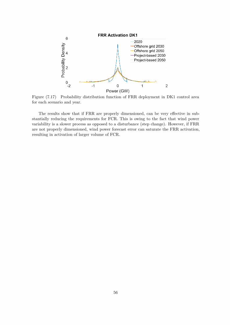
Figure (7.17) Probability distribution function of FRR deployment in DK1 control areafor each scenario and year.

The results show that if FRR are properly dimensioned, can be very effective in sub-stantially reducing the requirements for FCR. This is owing to the fact that wind powervariability is a slower process as opposed to a disturbance (step change). However, if FRRare not properly dimensioned, wind power forecast error can saturate the FRR activation,resulting in activation of larger volume of FCR.

56

Chapter 8

Conclusion

This report analyses a study in the operation of the power system of Continental Europeand Nordic synchronous areas with focusing on the Danish power system and its regionsDK1 and DK2. The study covers all the steps of the operation from the Day Ahead Markettil the the Real Time balancing of generation and demand. For that reason, a balancingtool chain has been developed. Furthermore, two scenarios of the future generation andtransmission capacity development - Project based and Offshore grid, are considered andsimulated for the North Sea countries in 2030 and 2050. The project-based and the offshoregrid scenarios represented two different approaches regarding the transmission structurebetween the North Sea countries of the near future.

The report analyses a) the value of offshore grid on balancing of forecast errors, b) theimpact of forecast errors on manual and automatic reserves and c) the quality of electricalfrequency in the near future considering high VRE penetration.

The simulation results clearly shows that the offshore grid scenario has very similarimpact on balancing of reserves to project based scenario. Since offshore grid scenario pro-vides additional values like increased security and flexibility as well as larger integration ofNorth Sea countries, having similar impact on balancing as that of project based, makesoffshore grid an recommendable option for future grid development. Additionally, real-timeimbalance in Nordic network is much lower in case of Offshore grid scenario as comparedto Project based scenario.

Day ahead market simulations for future shows higher amount of curtailment mainlypertaining to very high volume of installation of wind power. However, the volume of windpower curtailed is still low as compared to the total amount of wind power generation. Thisbeing the reason, there is no seasonal pattern in the curtailment of wind power in futurescenarios.

Simulations have shown that in future, hour ahead imbalance due to wind forecast errorincreases in Denmark mainly in DK1. However, the hour ahead imbalance for the wholesynchronous area does not increase much. Therefore, intra-hour balancing of Danish controlarea is largely supported from neighboring regions. Balancing cost which is highly drivenby CO2 prices in the simulation, increases substantially towards 2030. Balancing reservesin CE are largely provided by Natural Gas technologies whereas, in Nordic network, bal-

57

ancing reserves come from Hydro and Natural Gas. Balancing reserves in Denmark mainlycome from Natural Gas. However, wind power also increases their role in balancing processin future, mainly in down regulation but also in up regulation especially if wind power isalready curtailed in the day-ahead operation.

Real time imbalance seen by Nordic network increases multiple times in 2030 and 2050scenario as compared to 2020 scenario. Additionally, the real time imbalance in Offshoregrid scenario is much lower than that of Project based scenario. Nordic network is alsoexpected to have much lower inertia available in future scenarios as compared to 2020scenario. The requirement for automatic frequency restoration reserves increases manifoldin future scenarios as compared to 2020 scenario. Probabilistic dimensioning of frequencyrestoration reserves can be beneficial to mitigate the imbalances caused by wind powerforecast error mainly in Nordic network. Even with proper dimensioning of frequencyrestoration reserves, frequency containment reserve for normal operation in Nordic networkmight be required to be increased in future 2030 and 2050 scenario with very high share ofrenewables in the power system.

58

Bibliography

[1] J. Gea-Bermúdez, K. Das, L.-L. Pade, M. Koivisto, and P. Kanellas. (2019). NSON-DKday-ahead market operation analysis in the north sea region towards 2050 , TechnicalUniversity of Denmark, [Online]. Available: https://backend.orbit.dtu.dk/ws/files/202747832/NSON_DK_WP3_D3.1.pdf.

[2] M. Koivisto and J. Gea-Bermúdez. (2018). NSON-DK energy system scenarios – edi-tion 2, DTU Wind Energy, [Online]. Available: http : / / orbit . dtu . dk / files /160234729/NSON_DK_WP2_D2.1.Ed2_FINAL.pdf.

[3] K. Das, M. J. Koivisto, P. E. Sørensen, and J. Gea-Bermúdez, “Balancing challengesfor future north sea offshore network,” in 17th International Workshop on Large-ScaleIntegration of Wind Power into Power Systems as well as on Transmission Networksfor Offshore Wind Power Plants, Energynautics GmbH, 2018.

[4] M. Koivisto, K. Das, F. Guo, P. Sørensen, E. Nuño, N. Cutululis, and P. Maule.(2018). Using time series simulation tool for assessing the effects of variable renewableenergy generation on power and energy systems, WIREs Energy and Environment.https://doi.org/10.1002/wene.329.

[5] F. Wiese, R. Bramstoft, H. Koduvere, A. Pizarro Alonso, O. Balyk, J.G. Kirkerud,and H. Ravn. (2018). Balmorel open source energy system model, Energy StrategyReviews, 20, 26-34. https://doi.org/10.1016/j.esr.2018.01.003.

[6] European Commission, Study of the benefits of a meshed offshore grid in NorthernSeas region. (2014), [Online]. Available: http://ec.europa.eu/energy/en/content/benefits-meshed-offshore-grid-northern-seas-region.

[7] M. Koivisto et al., Using time series simulation tool for assessing the effects of variablerenewable energy generation on power and energy systems, Wiley InterdisciplinaryReviews: Energy and Environment, p. e329, 2019.

[8] J. Gea-Bermúdez, K. Das, L.-L. Pade, M. Koivisto, and P. Kanellas, NSON-DK Day-Ahead market operation analysis in the North Sea region towards 2050, English. Tech-nical University of Denmark, 2019, isbn: 978-87-93549-61-6.

[9] P. Kanellas, K. Das, P. E. Sørensen, and J. Gea-Bermudez, “Modelling the intra-hourpower system balancing of the danish power system for 2020, 2030 and 2050,” in 18thWind Integration Workshop, 2019.

[10] K. Das, M. Litong-Palima, P. Maule, and P. E. Sørensen, “Adequacy of operatingreserves for power systems in future european wind power scenarios,” in 2015 IEEEPower Energy Society General Meeting, 2015, pages 1–5.

59

https://backend.orbit.dtu.dk/ws/files/202747832/NSON_DK_WP3_D3.1.pdf

https://backend.orbit.dtu.dk/ws/files/202747832/NSON_DK_WP3_D3.1.pdf

http://orbit.dtu.dk/files/160234729/NSON_DK_WP2_D2.1.Ed2_FINAL.pdf

http://orbit.dtu.dk/files/160234729/NSON_DK_WP2_D2.1.Ed2_FINAL.pdf

http://ec.europa.eu/energy/en/content/benefits-meshed-offshore-grid-northern-seas-region

http://ec.europa.eu/energy/en/content/benefits-meshed-offshore-grid-northern-seas-region

[11] K. Das, M. Litong-Palima, P. Maule, M. Altin, A. D. Hansen, P. E. Sørensen, and H.Abildgaard, “Adequacy of frequency reserves for high wind power generation,” IETRenewable Power Generation, volume 11, number 8, pages 1286–1294, 2017.

[12] SVENSKA KRAFTNAT, Statnett. (2017). The nordic balancing concept, [Online].Available: https://www.statnett.no/globalassets/om-statnett/nyheter-og-pressemeldinger/nyhetsarkiv-2018/the-nordic-balancing-concept.pdf.

[13] FINGRID. (2019). Reserves and balancing power, [Online]. Available: https://www.fingrid . fi / en / electricity - market / reserves _ and _ balancing / #reserve -products.

[14] E. F. Sichani, “Frequency control in future nordic power system with high penetrationof wind power,” Master’s thesis, DTU Wind, Technical University of Denmark, 2017.

[15] Frequency Control in the European Power System Considering the OrganisationalStructure and Division of Responsibilities. (2016), [Online]. Available: https://doi.org/10.3929/ethz-a-010692129.

[16] Handbook, UCTE Operations. (2009). P1–policy 1: Load-frequency control and perfor-mance [c], [Online]. Available: https://www.entsoe.eu/fileadmin/user_upload/_library/publications/entsoe/Operation_Handbook/Policy_1_final.pdf.

[17] ENTSO-E. (2013). Network code on load frequency control and reserves (lfcr), [On-line]. Available: https : / / www . entsoe . eu / major - projects / network - code -development/load-frequency-control-reserves/Pages/default.aspx.

60

https://www.statnett.no/globalassets/om-statnett/nyheter-og-pressemeldinger/nyhetsarkiv-2018/the-nordic-balancing-concept.pdf

https://www.statnett.no/globalassets/om-statnett/nyheter-og-pressemeldinger/nyhetsarkiv-2018/the-nordic-balancing-concept.pdf

https://www.fingrid.fi/en/electricity-market/reserves_and_balancing/#reserve-products



https://doi.org/10.3929/ethz-a-010692129

https://doi.org/10.3929/ethz-a-010692129

https://www.entsoe.eu/fileadmin/user_upload/_library/publications/entsoe/Operation_Handbook/Policy_1_final.pdf

https://www.entsoe.eu/fileadmin/user_upload/_library/publications/entsoe/Operation_Handbook/Policy_1_final.pdf

https://www.entsoe.eu/major-projects/network-code-development/load-frequency-control-reserves/Pages/default.aspx

https://www.entsoe.eu/major-projects/network-code-development/load-frequency-control-reserves/Pages/default.aspx

Appendix A

Mathematical model formulationof Day Ahead Market Model inBalmorel

A.1 MethodologyThe temporal representation used consists of years y ∈ Y , which are disaggregated intoseasons s ∈ S which are composed of time steps t ∈ T . For the simulations of Day Aheadmarket the season represent days and time steps represent hours. Regarding the geograph-ical representation, there are three gradation: countries consisting of regions r ∈ R, whichare disaggregated into areas a ∈ A. Regions represent copperplate zones for electricitytransmission, whereas areas represent copperplate zones for heat transmission.

The methodology used to simulate the Day-Ahead market can be split in three groups:Storage and planned maintenance optimisation , Stochastic outage simulations and Day-Ahead optimisation. As already mentioned, the optimisations are performed with the en-ergy system model Balmorel and the VRE generation time series where calculated with thesimulation tool CorRES.

The Storage and planned maintenance optimisation is run in order to capture the de-cision that need to be made from the market participants based on future expectations ofmarket prices and not just on the next 24 hours. The maintenance time is technology spe-cific and the generators choose when they will be inoperative considering the losses comingfrom their absence from the market. In addition, in order to maximize their profit storageunits have to load during seasons with low prices and unload in seasons with high prices.These two decisions are made by running the Storage and planned maintenance optimisa-tion model for a full year, saving the results at the beginning of each season and forcingthem during the Day Ahead optimization.

In order to introduce the stochasticity of an unexpected operational problem in themodel the Stochastic outage simulation is used. The stochastic outages are modelled byconsidering the total capacity of a unit type in each area, the size of a single unit, theplanned maintenance, and the probability of suffering an outage. The outages are assumedto last 1 hour and Monte Carlo simulations are performed for every time step and unit.

61

The results of these simulation are also forced during the Day Ahead market optimization.

A.2 Mathematical model formulationA.2.1 Day-Ahead optimisation formulation

Objective function

The objective function is to minimize the operational costs of the studied system for eachtime step. In Day Ahead market the time steps considered in this optimisation correspondto one hour. Its year is optimized separately as the years are not linked. In this report, thesecosts have been aggregated into to fixed operational and maintenance costs (fom), variableoperational and maintenance costs (vom), unit commitment related costs (uc), emission taxcosts (emi), and transmission use costs (trans).

min∑y∈Y

cfomy + cvomy + cucy + cemiy + ctransy (A.1)

Fixed O&M costs

Fixed costs depict the annual availability cost to be paid regardless of the use of eachtechnology:

cfomy =∑a∈A

(∑g∈E

FCg,a,y · ηel · Cfomg

+∑

g∈H,g/∈CHP

FCg,a,y · ηh · Cfomg

)∀y ∈ Y

(A.2)

Variable Operational and Maintenance costs

Variable operation and maintenance costs depict fuel (f) consumption costs, as well asthe cost related with normal operation (oper) (e.g. consumption of auxiliary materials,maintenance, etc):

cvomy =∑a∈A

∑s∈S

∑t∈T

( ∑g∈G,g/∈PTOH

dfg,a,y,s,t · Cfg,a,y

+∑

g∈EL,g/∈CHP

pelg,a,y,s,t · Coperg

+∑

g∈H,g/∈CHP

phg,a,y,s,t · Coperg

+∑

g∈CHPdfg,a,y,s,t · Coper

g

)∀y ∈ Y

(A.3)

62

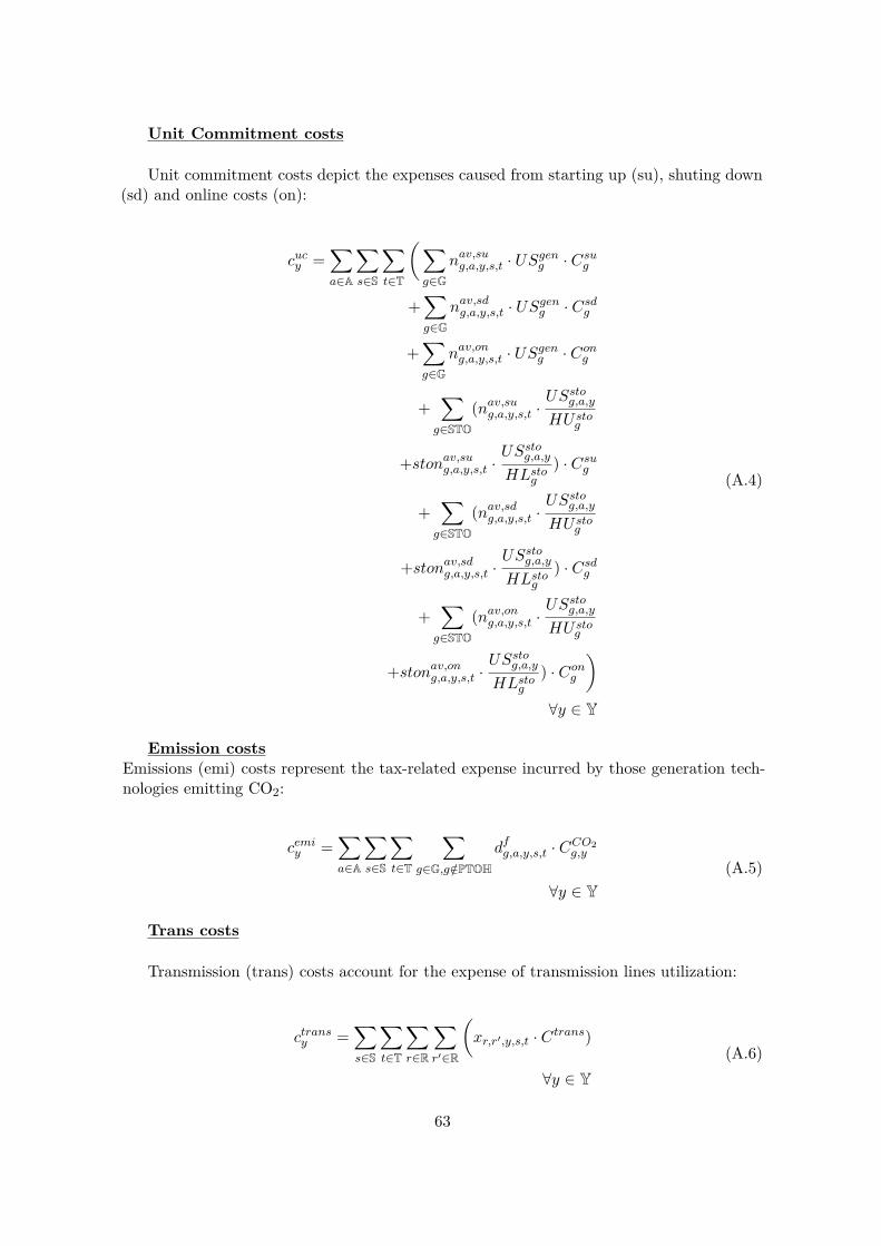
Unit Commitment costs

Unit commitment costs depict the expenses caused from starting up (su), shuting down(sd) and online costs (on):

cucy =∑a∈A

∑s∈S

∑t∈T

(∑g∈G

nav,sug,a,y,s,t · USgen

g · Csug

+∑g∈G

nav,sdg,a,y,s,t · USgen

g · Csdg

+∑g∈G

nav,ong,a,y,s,t · USgen

g · Cong

+∑

g∈STO(nav,su

g,a,y,s,t ·USsto

g,a,y

HU stog

+stonav,sug,a,y,s,t ·

USstog,a,y

HLstog

) · Csug

+∑

g∈STO(nav,sd

g,a,y,s,t ·USsto

g,a,y

HU stog

+stonav,sdg,a,y,s,t ·

USstog,a,y

HLstog

) · Csdg

+∑

g∈STO(nav,on

g,a,y,s,t ·USsto

g,a,y

HU stog

+stonav,ong,a,y,s,t ·

USstog,a,y

HLstog

) · Cong

)∀y ∈ Y

(A.4)

Emission costsEmissions (emi) costs represent the tax-related expense incurred by those generation tech-nologies emitting CO2:

cemiy =

∑a∈A

∑s∈S

∑t∈T

∑g∈G,g/∈PTOH

dfg,a,y,s,t · CCO2g,y

∀y ∈ Y(A.5)

Trans costs

Transmission (trans) costs account for the expense of transmission lines utilization:

ctransy =∑s∈S

∑t∈T

∑r∈R

∑r′∈R

(xr,r′,y,s,t · Ctrans)

∀y ∈ Y(A.6)

63

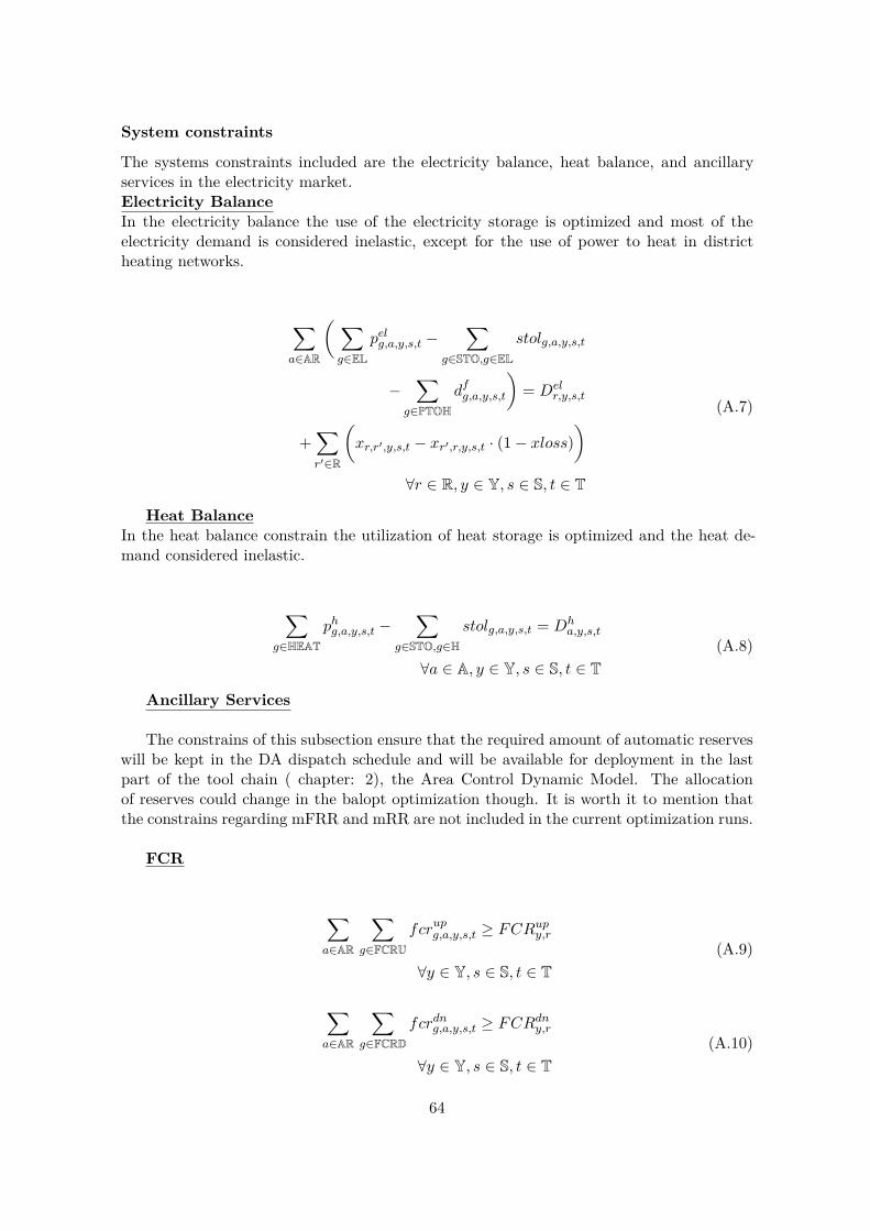
System constraints

The systems constraints included are the electricity balance, heat balance, and ancillaryservices in the electricity market.Electricity BalanceIn the electricity balance the use of the electricity storage is optimized and most of theelectricity demand is considered inelastic, except for the use of power to heat in districtheating networks.

∑a∈AR

( ∑g∈EL

pelg,a,y,s,t −∑

g∈STO,g∈ELstolg,a,y,s,t

−∑

g∈PTOHdfg,a,y,s,t

)= Del

r,y,s,t

+∑r′∈R

(xr,r′,y,s,t − xr′,r,y,s,t · (1− xloss)

)∀r ∈ R, y ∈ Y, s ∈ S, t ∈ T

(A.7)

Heat BalanceIn the heat balance constrain the utilization of heat storage is optimized and the heat de-mand considered inelastic.

∑g∈HEAT

phg,a,y,s,t −∑

g∈STO,g∈Hstolg,a,y,s,t = Dh

a,y,s,t

∀a ∈ A, y ∈ Y, s ∈ S, t ∈ T(A.8)

Ancillary Services

The constrains of this subsection ensure that the required amount of automatic reserveswill be kept in the DA dispatch schedule and will be available for deployment in the lastpart of the tool chain ( chapter: 2), the Area Control Dynamic Model. The allocationof reserves could change in the balopt optimization though. It is worth it to mention thatthe constrains regarding mFRR and mRR are not included in the current optimization runs.

FCR

∑a∈AR

∑g∈FCRU

fcrupg,a,y,s,t ≥ FCRupy,r

∀y ∈ Y, s ∈ S, t ∈ T(A.9)

∑a∈AR

∑g∈FCRD

fcrdng,a,y,s,t ≥ FCRdny,r

∀y ∈ Y, s ∈ S, t ∈ T(A.10)

64

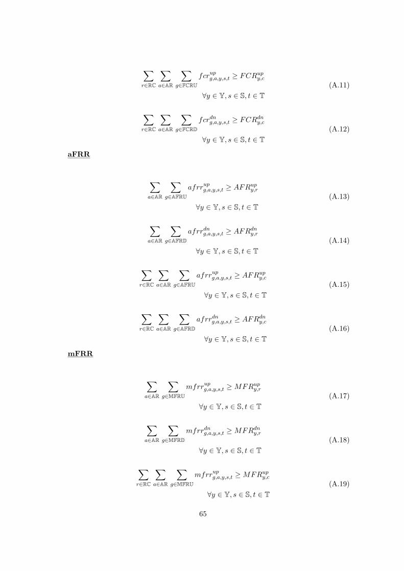
∑r∈RC

∑a∈AR

∑g∈FCRU

fcrupg,a,y,s,t ≥ FCRupy,c

∀y ∈ Y, s ∈ S, t ∈ T(A.11)

∑r∈RC

∑a∈AR

∑g∈FCRD

fcrdng,a,y,s,t ≥ FCRdny,c

∀y ∈ Y, s ∈ S, t ∈ T(A.12)

aFRR

∑a∈AR

∑g∈AFRU

afrrupg,a,y,s,t ≥ AFRupy,r

∀y ∈ Y, s ∈ S, t ∈ T(A.13)

∑a∈AR

∑g∈AFRD

afrrdng,a,y,s,t ≥ AFRdny,r

∀y ∈ Y, s ∈ S, t ∈ T(A.14)

∑r∈RC

∑a∈AR

∑g∈AFRU

afrrupg,a,y,s,t ≥ AFRupy,c

∀y ∈ Y, s ∈ S, t ∈ T(A.15)

∑r∈RC

∑a∈AR

∑g∈AFRD

afrrdng,a,y,s,t ≥ AFRdny,c

∀y ∈ Y, s ∈ S, t ∈ T(A.16)

mFRR

∑a∈AR

∑g∈MFRU

mfrrupg,a,y,s,t ≥ MFRupy,r

∀y ∈ Y, s ∈ S, t ∈ T(A.17)

∑a∈AR

∑g∈MFRD

mfrrdng,a,y,s,t ≥ MFRdny,r

∀y ∈ Y, s ∈ S, t ∈ T(A.18)

∑r∈RC

∑a∈AR

∑g∈MFRU

mfrrupg,a,y,s,t ≥ MFRupy,c

∀y ∈ Y, s ∈ S, t ∈ T(A.19)

65

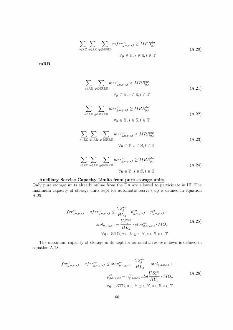
∑r∈RC

∑a∈AR

∑g∈MFRD

mfrrdng,a,y,s,t ≥ MFRdny,c

∀y ∈ Y, s ∈ S, t ∈ T(A.20)

mRR

∑a∈AR

∑g∈MRRU

mrrupg,a,y,s,t ≥ MRRupy,r

∀y ∈ Y, s ∈ S, t ∈ T(A.21)

∑a∈AR

∑g∈MRRD

mrrdng,a,y,s,t ≥ MRRdny,r

∀y ∈ Y, s ∈ S, t ∈ T(A.22)

∑r∈RC

∑a∈AR

∑g∈MRRU

mrrupg,a,y,s,t ≥ MRRupy,c

∀y ∈ Y, s ∈ S, t ∈ T(A.23)

∑r∈RC

∑a∈AR

∑g∈MRRD

mrrdng,a,y,s,t ≥ MRRdny,c

∀y ∈ Y, s ∈ S, t ∈ T(A.24)

Ancillary Service Capacity Limits from pure storage unitsOnly pure storage units already online from the DA are allowed to participate in IH. Themaximum capacity of storage units kept for automatic resrve’s up is defined in equationA.25.

fcrupg,a,y,s,t + afrrupg,a,y,s,t ≤USsto

g

HUg· non

g,a,y,s,t − pelg,a,y,s,t+

stolg,a,y,s,t −USsto

g

HLg· stonon

g,a,y,s,t ·MOg

∀g ∈ STO, a ∈ A, y ∈ Y, s ∈ S, t ∈ T

(A.25)

The maximum capacity of storage units kept for automatic resrve’s down is defined inequation A.28.

fcrdng,a,y,s,t + afrrdng,a,y,s,t ≤ stonong,a,y,s,t ·

USstog

HLg− stolg,a,y,s,t+

pelg,a,y,s,t − nong,a,y,s,tcdot

USstog

HUg·MOg

∀g ∈ STO, a ∈ A, y ∈ Y, s ∈ S, t ∈ T

(A.26)

66

Ancillary Service Energy Limits from pure storage units

socg,a,y,s,t + TLs,t · (stolg,a,y,s,t −pelg,a,y,s,tηstog

) ≥

fcrupg,a,y,s,t + afrrupg,a,y,s,tηstog

(A.27)

FCg,a,y

ηstog

− socg,a,y,s,t + TLs,t ·(stolg,a,y,s,t −

pelg,a,y,s,tηstog

)≥

fcrdng,a,y,s,t + afrrdng,a,y,s,t

(A.28)

Technological constraints for dispatchable generation units

Dispatchable technologies include power-only, CHP, boilers, heat pumps, geothermal, andhydroelectric power with reservoirs. These units are subject to several technical constraints.

Available unitsThe maximum number of available units for generation depends on the installed capacity,unit size, and Availability Factor (AF):

FCg,a,y

USgeng

·AFg,a,y,s,t ≥ nav,ong,a,y,s,t

∀g ∈ GD, a ∈ A, y ∈ Y, s ∈ S, t ∈ T(A.29)

The parameter AF depends on installed capacity, unit size, units under planned main-tenance and units under forced outage:

AFg,a,y,s,t = max

{1−

USgeng · (nnav,pm

g,a,y,s + nnav,sog,a,y,s,t)

FCg,a,y, 0

}∀g ∈ GD, a ∈ A, y ∈ Y, s ∈ S, t ∈ T

(A.30)

The number of units on planned maintenance is taken from the storage and plannedmaintenance optimization. The number of units under forced outage is taken from thestochastic outage simulations.

Fuel consumption limits

The consumption of fuel from the generators is modeled through the constrains presentedin this subsection. The maximum and minimum fuel consumption constrains are presentedin equations A.31 and A.32 respectively.

USgeng · nav,on

g,a,y,s,t ≥ dfg,a,y,s,t

∀g ∈ GD, a ∈ A, y ∈ Y, s ∈ S, t ∈ T(A.31)

67

dfg,a,y,s,t ≥ USgeng · nav,on

g,a,y,s,t ·MOg

∀g ∈ GD, a ∈ A, y ∈ Y, s ∈ S, t ∈ T(A.32)

Ramping constraints

The constrains representing the ramping of generators are presented bellow. Rampingup and ramping down is simulated based on the equations A.33 and A.34 respectively.

dfg,a,y,s,t − dfg,a,y,s,t−1 ≤USgen

g · (nav,ong,a,y,s,t − nav,su

g,a,y,s,t) ·RRupg

∀g ∈ PO, a ∈ A, y ∈ Y, s ∈ S, t ∈ T

(A.33)

dfg,a,y,s,t−1 − dfg,a,y,s,t ≤

USgeng · (nav,on

g,a,y,s,t + nav,sdg,a,y,s,t) ·RRdown

g

∀g ∈ PO, a ∈ A, y ∈ Y, s ∈ S, t ∈ T

(A.34)

Minimum on/off time constraints

Some of the generators have to be on or off for at least a pre-defined minimum timebefore their state is changed. The minimum on and off time constrains are presented inequations A.35 and A.36 respectively.

MUTg∑t′=1

nav,sug,a,y,s,t−t′ ≤ nav,on

g,a,y,s,t

∀g ∈ PO, a ∈ A, y ∈ Y, s ∈ S, t ∈ T

(A.35)

MDTg∑t′=1

nav,sdg,a,y,s,t−t′ ≤

FCg,a,y

USgeng

− nav,ong,a,y,s,t

∀g ∈ PO, a ∈ A, y ∈ Y, s ∈ S, t ∈ T

(A.36)

Logical conditions

nav,ong,a,y,s,t − nav,on

g,a,y,s,t−1 = nav,sug,a,y,s,t − nav,sd

g,a,y,s,t

∀g ∈ GD, a ∈ A, y ∈ Y, s ∈ S, t ∈ T(A.37)

In order to reflect the discrete nature of the generation units that are part of the energysystem, the following variables are restricted to be integer variables. In case that reducingthe computational time is essential, this constrain can be relaxed and it’s variables becomecontinuous.

68

nav,ong,a,y,s,t, n

av,sug,a,y,s,t, n

av,sdg,a,y,s,t ∈ Z+

∀g ∈ GD, a ∈ A, y ∈ Y, s ∈ S, t ∈ T(A.38)

Specific technological constraints for power only thermal plants

The installed capacity represents the maximum net generation of power. Technologiesinvolved are gas and steam turbines, engines, and combined cycles.

dfg,a,y,s,t · ηelg ≥ pelg,a,y,s,t

∀g ∈ PO, a ∈ A, y ∈ Y, s ∈ S, t ∈ T(A.39)

Specific technological constraints for heat only producers

The installed capacity represents the maximum net generation of heat. Technologiesinvolved are fuel boilers and Power-to-Heat units.

dfg,a,y,s,t · ηhg = phg,a,y,s,t

∀g ∈ HO, a ∈ A, y ∈ Y, s ∈ S, t ∈ T(A.40)

Specific technological constraints for Combined Heat and Power thermal plants

Back pressure technologies present linear relation between electricity and heat generation(CB line).

peg,a,y,s,t = phg,a,y,s,t · CBg

∀g ∈ BP, a ∈ A, y ∈ Y, s ∈ S, t ∈ T(A.41)

Their fuel demand depends on the electrical efficiency and production:

dfg,a,y,s,t · ηelg = peg,a,y,s,t

∀g ∈ BP, a ∈ A, y ∈ Y, s ∈ S, t ∈ T(A.42)

On the other hand, extraction power plans have a more flexible range of operation ofheat and power. They are capable of producing power without producing heat, but nototherwise. The CB and CV (iso-fuel) parameter define the operational range:

peg,a,y,s,t ≥ phg,a,y,s,t · CBg

∀g ∈ EXT, a ∈ A, y ∈ Y, s ∈ S, t ∈ T(A.43)

USgeng · non

g,a,y,s,t · ηelg ≥ peg,a,y,s,t + phg,a,y,s,t · CVg

∀g ∈ EXT, a ∈ A, y ∈ Y, s ∈ S, t ∈ T(A.44)

69

dfg,a,y,s,t · ηelg = peg,a,y,s,t + phg,a,y,s,t · CVg

∀g ∈ BP, a ∈ A, y ∈ Y, s ∈ S, t ∈ T(A.45)

Specific technological constraints for hydro power plants with seasonal inflow

Hydroelectric power with reservoirs are modelled as a generation technology linked tostorage with limited energy capacity and that receives seasonal energy inflows. The modeloptimizes the production and level of storage along the year, with the condition that thelevel of the storage at the beginning of the simulated year equals the level at the end. Thelevel at the beginning of each season is forced from the storage and planned maintenanceoptimisation.

hsla,y,s+1 ≥ hsla,y,s +HIa,s

+∑t∈T

∑g∈HYD

TLs,t ·pelg,a,y,s,t

ηelg

∀a ∈ A, y ∈ Y, s ∈ S

(A.46)

HSLa,s ≥ hsla,y,s

∀a ∈ A, y ∈ Y, s ∈ S(A.47)

HSLa,s ≤ hsla,y,s

∀a ∈ A, y ∈ Y, s ∈ S(A.48)

Technological constraints for pure storage units

Those storage units that do not receive inflow except from the active loading are definedas pure storage units. Examples of these technologies are hydro pumping, power batteries,and hot water tanks, or pit heat storage.The main equation for pure storage is the storage balance, which for these technologies iscalculated for every t. The level at the beginning of each season is forced from the storageand planned maintenance optimisation. Fuel demand equals in this case electricity, or heat,production:

Storage balance

The equation B.4 simulates the state of charge of pure storage technologies.

socg,a,y,s,t+1 = socg,a,y,s,t

+TLs,t · (stolg,a,y,s,t −pfg,a,y,s,tηstog

)

∀g ∈ STO, a ∈ A, y ∈ Y, s ∈ S, t ∈ T

(A.49)

70

Available units

The equations A.50 and A.51 model the maximum number of units available for unload-ing and loading for pure storage technologies respectively.

ECg,a,y

USstog

·AFg,a,y,s,t ≥ nav,ong,a,y,s,t

∀g ∈ STO, a ∈ A, y ∈ Y, s ∈ S, t ∈ T(A.50)

ECg,a,y

USstog

·AFg,a,y,s,t ≥ stonav,ong,a,y,s,t

∀g ∈ STO, a ∈ A, y ∈ Y, s ∈ S, t ∈ T(A.51)

The availability factor is constraint by the storage itself, so the assumption is that if thestorage is not available, it is not available for loading nor unloading.

AFg,a,y,s,t = max

{1−

USg · (nnav,pmg,a,y,s + nnav,so

g,a,y,s,t)

KGg

, 0

}∀g ∈ STO, a ∈ A, y ∈ Y, s ∈ S, t ∈ T

(A.52)

Storage loading and unloading limits

The maximum allowed unloading of pure storage units is defined in equations A.53 andA.54.

USstog

HUg· nav,on

g,a,y,s,t ≥ pelg,a,y,s,t

∀g ∈ STOEL, a ∈ A, y ∈ Y, s ∈ S, t ∈ T(A.53)

USstog

HUg· nav,on

g,a,y,s,t ≥ phg,a,y,s,t

∀g ∈ STOH, a ∈ A, y ∈ Y, s ∈ S, t ∈ T(A.54)

The maximum allowed loading of pure storage units is defined in equation A.55.

USstog

HLg· stonon

g,a,y,s,t ≥ stolg,a,y,s,t

∀g ∈ STO, a ∈ A, y ∈ Y, s ∈ S, t ∈ T(A.55)

The minimum allowed unloading of pure storage units is defined in equations A.56 andA.57.

USstog

HUg· non

g,a,y,s,t ·MOg· ≤ pelg,a,y,s,t

∀g ∈ STOEL, a ∈ A, y ∈ Y, s ∈ S, t ∈ T(A.56)

71

USstog

HUg· non

g,a,y,s,t ·MOg ≤ phg,a,y,s,t

∀g ∈ STOH, a ∈ A, y ∈ Y, s ∈ S, t ∈ T(A.57)

The minimum allowed loading of pure storage units is defined in equation A.58.

USstog

HLg· stonon

g,a,y,s,t ·MOg ≥ stolg,a,y,s,t

∀g ∈ STO, a ∈ A, y ∈ Y, s ∈ S, t ∈ T(A.58)

Ramping constraints

The constrains modeling the ramping up of pure storage units during unloading pre-sented in equations A.59 and A.60.

pelg,a,y,s,t − pelg,a,y,s,t−1 ≤USsto

g

HUg· (nav,on

g,a,y,s,t − nav,sug,a,y,s,t) ·RRup

g

∀g ∈ STO, g ∈ EL, a ∈ A, y ∈ Y, s ∈ S, t ∈ T

(A.59)

phg,a,y,s,t − phg,a,y,s,t−1 ≤USsto

g

HUg· (nav,on


g

∀g ∈ STO, g ∈ HEAT, a ∈ A, y ∈ Y, s ∈ S, t ∈ T

(A.60)

The ramping up of pure storage units during loading is modeled through equation A.61.

stolg,a,y,s,t − stolg,a,y,s,t−1 ≤USsto

g

HLg· (nav,on


g

∀g ∈ STO, a ∈ A, y ∈ Y, s ∈ S, t ∈ T

(A.61)

Similarly, the modeling of ramping down in case of unloading is done from the constrainsA.59 and A.60.

pelg,a,y,s,t−1 − pelg,a,y,s,t ≤USsto

g

HUg· (nav,on

g,a,y,s,t − nav,sug,a,y,s,t) ·RRdown

g

∀g ∈ STO, g ∈ EL, a ∈ A, y ∈ Y, s ∈ S, t ∈ T

(A.62)

72

phg,a,y,s,t−1 − phg,a,y,s,t ≤USsto

g

HUg· (nav,on


g

∀g ∈ STO, g ∈ HEAT, a ∈ A, y ∈ Y, s ∈ S, t ∈ T

(A.63)

The ramping down of pure storage units during loading is simulated through the equationA.64.

stolg,a,y,s,t−1 − stolg,a,y,s,t ≤USsto

g

HLg· (nav,on


g

∀g ∈ STO, a ∈ A, y ∈ Y, s ∈ S, t ∈ T

(A.64)

Minimum on/off time constraints

The minimum on time during unloading and loading is defined through the equationsA.65 and A.66 respectively.

MUTg∑t′=1

nav,sug,a,y,s,t−t′ ≤ nav,on

g,a,y,s,t

∀g ∈ STO, a ∈ A, y ∈ Y, s ∈ S, t ∈ T

(A.65)

MUTg∑t′=1

stonav,sug,a,y,s,t−t′ ≤ stonav,on

g,a,y,s,t

∀g ∈ STO, a ∈ A, y ∈ Y, s ∈ S, t ∈ T

(A.66)

The minimum off time during unloading and loading is defined through the equationsA.67 and A.68 respectively.

MDTg∑t′=1

nav,sdg,a,y,s,t−t′ ≤

ECg,a,y

USstog

− nav,ong,a,y,s,t

∀g ∈ STO, a ∈ A, y ∈ Y, s ∈ S, t ∈ T

(A.67)

MDTg∑t′=1

stonav,sdg,a,y,s,t−t′ ≤

ECg,a,y

USstog

− stonav,ong,a,y,s,t

∀g ∈ STO, a ∈ A, y ∈ Y, s ∈ S, t ∈ T

(A.68)

Logical conditions

73

Logical conditions regarding the unloadin and loading procedure of pure storage unitsare presented in equations A.69 and A.70 respectively.

nav,ong,a,y,s,t − nav,on

g,a,y,s,t−1 = nav,sug,a,y,s,t − nav,sd

g,a,y,s,t

∀g ∈ STO, a ∈ A, y ∈ Y, s ∈ S, t ∈ T(A.69)

stonav,ong,a,y,s,t − stonav,on

g,a,y,s,t−1 = stonav,sug,a,y,s,t + stonav,sd

g,a,y,s,t

∀g ∈ STO, a ∈ A, y ∈ Y, s ∈ S, t ∈ T(A.70)

In order to reflect the discrete nature of the storage units that are part of the energysystem, the following variables are restricted to be integer variables. In accordance withthe Logical conditions of dispatchable units, this constrain can be also relaxed by definingthe variables as continuous and reduce the computational time.

stonav,ong,a,y,s,t, ston

av,sug,a,y,s,t, ston

av,sdg,a,y,s,t ∈ Z+

∀g ∈ STO, a ∈ A, y ∈ Y, s ∈ S, t ∈ T(A.71)

Specific technological constraints for intermittent generation units

Non-dispatchable technologies included are solar PV, solar heating, wind onshore and off-shore, and hydro run of river.

Available electricity for generation is a function of the installed capacity and the timeseries in a given area

AEg,a,y,s,t ≥ pelg,a,y,s,t

∀g ∈ GI, g ∈ E, a ∈ A, y ∈ Y, s ∈ S, t ∈ T(A.72)

Likewise, available heat for generation is a function of the installed capacity and thetime series in a given area

AHg,a,y,s,t ≥ phg,a,y,s,t

∀g ∈ GI, g ∈ H, a ∈ A, y ∈ Y, s ∈ S, t ∈ T(A.73)

Power transmission constraints

Electricity exchange between neighboring regions is allowed but limited to the availabletransmission capacity. The available transmission capacity is calculated in each time stepas the product of the Net Transfer Capacity and the availability of each connection in thattime step.

TCr,r′,y,s,t · TCRr,r′,y,s,t ≥ xr,r′,y,s,t

∀r ∈ R, r′ ∈ R, y ∈ Y, s ∈ S, t ∈ T(A.74)

A.2.2 Storage and planned maintenance optimisation formulationThe code is almost the same as the one in section A.2.1, with a few exceptions.

74

Available units

The first exception is related to the availability of the units, which is endogenised in thisoptimisation. Equations A.29, A.50, and A.51 are replaced with equations A.75, A.76, A.77,respectively. The equations calculating the availability factor (A.29 and A.52) are not usedin this optimisation.

FCg,a,y

USgeng

− nnav,pmg,a,y,s ≥ nav,on

g,a,y,s,t

∀g ∈ GD, a ∈ A, y ∈ Y, s ∈ S, t ∈ T(A.75)

ECg,a,y

USstog

− nnav,pmg,a,y,s ≥ nav,on

g,a,y,s,t

∀g ∈ STO, a ∈ A, y ∈ Y, s ∈ S, t ∈ T(A.76)

ECg,a,y

USstog

− nnav,pmg,a,y,s ≥ stonav,on

g,a,y,s,t

∀g ∈ STO, a ∈ A, y ∈ Y, s ∈ S, t ∈ T(A.77)

Additionally, the maximum amount of units on maintenance is limited by the totalnumber of units

FCg,a,y

USgeng

≥ nnav,pmg,a,y,s

∀g ∈ GD, a ∈ A, y ∈ Y, s ∈ S, t ∈ T(A.78)

ECg,a,y

USstog

≥ nnav,pmg,a,y,s

∀g ∈ STO, a ∈ A, y ∈ Y, s ∈ S, t ∈ T(A.79)

Yearly maintenance requirement

The equations A.80 and A.81 guarantee the hour of maintenance per unit is respected duringthe year:

∑s∈S

nnav,pm,sug,a,y,s · SLs = MMTg ·

FCg,a,y

USgeng

∀g ∈ GD, a ∈ A, y ∈ Y,(A.80)

∑s∈S

nnav,pm,sug,a,y,s · SLs = MMTg ·

ECg,a,y

USstog

∀g ∈ STO, a ∈ A, y ∈ Y,(A.81)

75

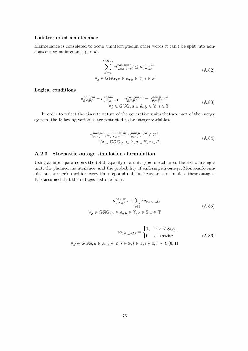
Uninterrupted maintenance

Maintenance is considered to occur uninterrupted,in other words it can’t be split into non-consecutive maintenance periods:

MMTg∑s′=1

nnav,pm.sug,a,y,s−s′ ≤ nnav,pm

g,a,y,s

∀g ∈ GGG, a ∈ A, y ∈ Y, s ∈ S

(A.82)

Logical conditions

nnav,pmg,a,y,s − nav,pm

g,a,y,s−1 = nnav,pm,sug,a,y,s − nnav,pm,sd

g,a,y,s

∀g ∈ GGG, a ∈ A, y ∈ Y, s ∈ S(A.83)

In order to reflect the discrete nature of the generation units that are part of the energysystem, the following variables are restricted to be integer variables.

nnav,pmg,a,y,s , nnav,pm,su

g,a,y,s , nnav,pm,sdg,a,y,s ∈ Z+

∀g ∈ GGG, a ∈ A, y ∈ Y, s ∈ S(A.84)

A.2.3 Stochastic outage simulations formulationUsing as input parameters the total capacity of a unit type in each area, the size of a singleunit, the planned maintenance, and the probability of suffering an outage, Montecarlo sim-ulations are performed for every timestep and unit in the system to simulate these outages.It is assumed that the outages last one hour.

nnav,sog,a,y,s,t =

∑i∈I

sog,a,y,s,t,i

∀g ∈ GGG, a ∈ A, y ∈ Y, s ∈ S, t ∈ T(A.85)

sog,a,y,s,t,i =

{1, if x ≤ SOg,i

0, otherwise∀g ∈ GGG, a ∈ A, y ∈ Y, s ∈ S, t ∈ T, i ∈ I, x ∼ U(0, 1)

(A.86)

76

Appendix B

Mathematical model formulationof Intra-hour Market Model inOptiBal

B.1 MethodologyThe OptiBal model receives as input the hour ahead wind forecast simulations in temporalresolution of 5 minutes from CorRES and the hourly generation schedule from Balmorel.The main purpose of this model is to calculate the required adjustments from non VREgenerators in order to counteract the imbalance occurred due to the mismatch of the DAwind dispatches and the new wind generation forecasts.

OptiBal is created as an add-on in the already existing Balmorel model. For that reason,the same methodology and structure of Balmorel was kept also in OptiBal. The temporalrepresentation in OptiBal similarly to Balmorel consists of years y ∈ Y , which are disaggre-gated into seasons s ∈ S which are composed of time steps t ∈ T. In contrast with the DayAhead optimization, for the simulations of the Intra Hour balancing market the seasonsrepresent hours and time steps represent 5 minute segments. The same three gradations(countries,regions,areas) for the geographical representation that are used in Balmorel arealso used in OptiBal’s algorithm. Again there are two types of generators participating inthe Intra Hour market, the dispatchable generators and the non-dispatchable which obvi-ously consist from the same technologies as in Day Ahead market. The algorithm used inOptiBal is identical with the one used in Balmorel with few exceptions which are describedin B.2. The objective function, the constrains regarding the system operation and all thetechnological constrains of dispatchable and non-dispatchable generators are used as pre-sented in chapter 5.

The methodology used to simulate the Intra Hour market can be split in two groups:Fixing Balancing Variables and the Balancing Market optimization.

The Intra Hour balancing market optimisation is performed on a hourly basis. Theresults are linked from hour to hour meaning that the results of the previous hour maylimit the results in the next hour. This limitation is highly dependent on the flexibility ofthe different units. The flexibility of the units, endogenously from the model, determines

77

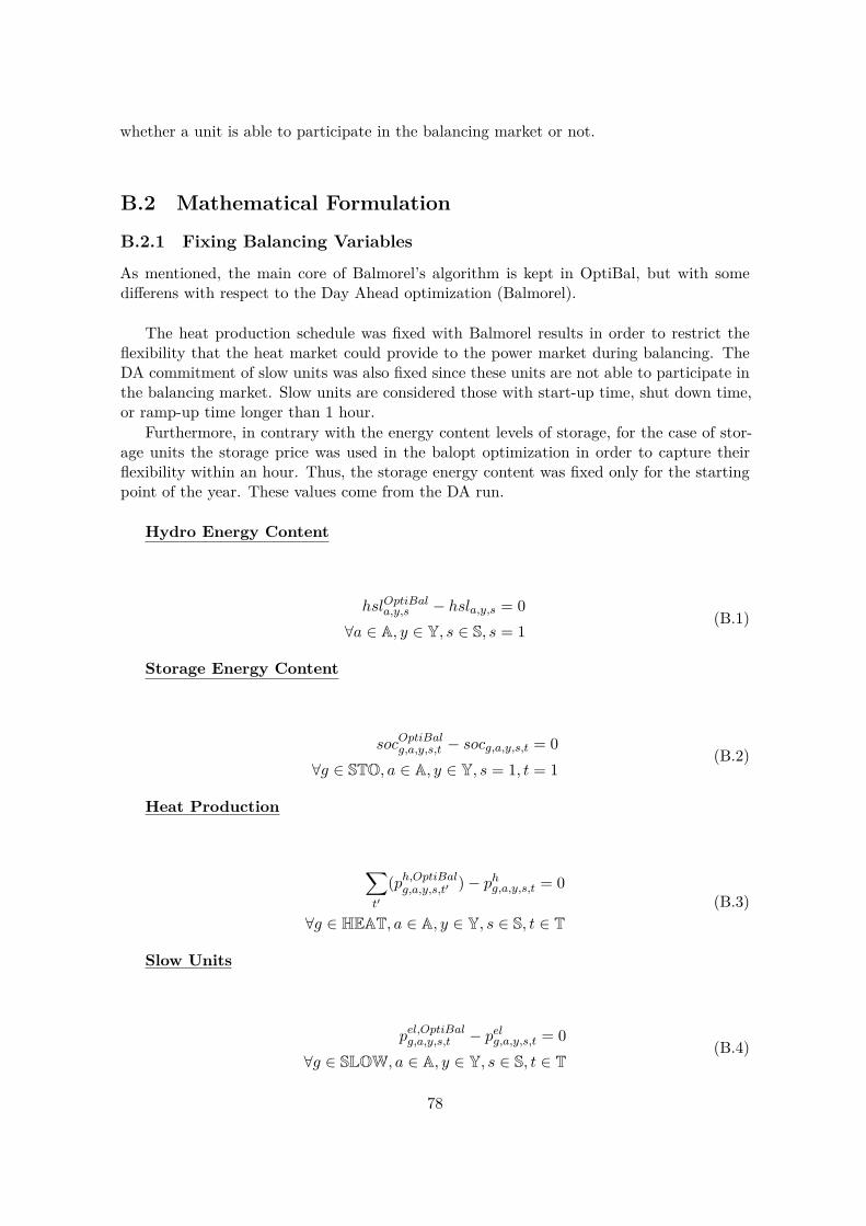
whether a unit is able to participate in the balancing market or not.

B.2 Mathematical Formulation

B.2.1 Fixing Balancing Variables

As mentioned, the main core of Balmorel’s algorithm is kept in OptiBal, but with somedifferens with respect to the Day Ahead optimization (Balmorel).

The heat production schedule was fixed with Balmorel results in order to restrict theflexibility that the heat market could provide to the power market during balancing. TheDA commitment of slow units was also fixed since these units are not able to participate inthe balancing market. Slow units are considered those with start-up time, shut down time,or ramp-up time longer than 1 hour.

Furthermore, in contrary with the energy content levels of storage, for the case of stor-age units the storage price was used in the balopt optimization in order to capture theirflexibility within an hour. Thus, the storage energy content was fixed only for the startingpoint of the year. These values come from the DA run.

Hydro Energy Content

hslOptiBala,y,s − hsla,y,s = 0

∀a ∈ A, y ∈ Y, s ∈ S, s = 1(B.1)

Storage Energy Content

socOptiBalg,a,y,s,t − socg,a,y,s,t = 0

∀g ∈ STO, a ∈ A, y ∈ Y, s = 1, t = 1(B.2)

Heat Production

∑t′

(ph,OptiBalg,a,y,s,t′ )− phg,a,y,s,t = 0

∀g ∈ HEAT, a ∈ A, y ∈ Y, s ∈ S, t ∈ T(B.3)

Slow Units

pel,OptiBalg,a,y,s,t − pelg,a,y,s,t = 0

∀g ∈ SLOW, a ∈ A, y ∈ Y, s ∈ S, t ∈ T(B.4)

78

B.2.2 Balancing optimizationThe OptiBal’s optimization part is exactly the same with Balmorel meaning that the ob-jective function, the system’s and the technological constrains of dispatchable, storage andVRE units are identical as in A.2.1, A.2.1, A.2.1, A.2.1 and A.2.1 respectively.

79

DTU Wind Energy is a department of the Technical University of Denmark with a unique integration of research, education, innovation and public/private sector consulting in the field of wind energy. Our activities develop new opportunities and technology for the global and Danish exploitation of wind energy. Research focuses on key technical-scientific fields, which are central for the development, innovation and use of wind energy and provides the basis for advanced education at the education.

We have more than 240 staff members of which approximately 60 are PhD students. Research is conducted within nine research programmes organized into three main topics: Wind energy systems, Wind turbine technology and Basics for wind energy.

Technical University of Denmark Department of Wind Energy Frederiksborgvej 399 Building 118 4000 Roskilde Denmark Telephone 46 77 50 85 [email protected] www.vindenergi.dtu.dk

Balancing Tool Chain: Balancing and automatic control in ...

Documents

Transcript of Balancing Tool Chain: Balancing and automatic control in ...