Balance Sheets and Exchange Rate Policy∗

Luis Felipe Cespedes† Roberto Chang‡ Andres Velasco§

Revised January 2004

Abstract

We study the relation among exchange rates, balance sheets, and macro-economic outcomes in a small open economy model. Entrepreneurial networth determines the risk premium on external financing, as in Bernankeand Gertler (1989). Because debts are in foreign currency, the impact of anadverse foreign shock is magnified by the increased debt burden due to theassociated real devaluation. But the devaluation also improves the assetside of the balance sheet, since it shifts demand toward domestic goods,increasing the return earned by entrepreneurs. Hence, the combination offinancial imperfections and foreign currency debts need not make devalua-tion contractionary, contrary to conjectures in recent literature. Regardless,the fall in investment, output and employment in response to an adverseshock is larger under fixed exchange rates than under flexible rates. In fact,flexible exchange rates Pareto dominate fixed rates and maximize socialwelfare.

∗We are grateful to Alberto Alesina, Abhijit Banerjee, Ricardo Caballero, Guillermo Calvo,Ricardo Hausmann, Paul Krugman, Enrique Mendoza, Richard Rogerson, Lars Svensson, threeanonymous referees and to participants at the Hoover Institution conference on Currency Unions,the Lacea Annual Meeting, and seminars at Harvard, Penn State, Princeton, Stanford, Univer-sity of Virginia, UC Berkeley, UC Santa Cruz, the New York Fed, and the Federal Reserve Boardfor useful comments. Chang and Velasco are grateful to the National Science Foundation forfinancial support. Logistical support from the Harvard Center for International Development isalso acknowledged with thanks. Any shortcomings are ours alone.

†Central Bank of Chile. Email: lcespede@bcentral.cl.‡Rutgers University. Email: chang@economics.rutgers.edu.§Harvard University and NBER. Email: andres velasco@harvard.edu.

1 Introduction

In conventional textbook accounts, expansionary monetary policy and depre-ciation of the currency are optimal in response to an adverse foreign shock.1

But if an economy has a large debt denominated in foreign currency, then aweaker local currency can also exacerbate debt-service difficulties and wreckthe balance sheets of domestic banks and firms. This channel may implythat devaluations are contractionary, not expansionary. As documented byHausmann et al (2000) and Calvo and Reinhart (2002), balance sheet effectshave emerged as a prime reason why many central banks are reluctant toallow their currencies to devalue in response to external shocks.Such concerns have generated an active policy debate, but the issue is

only beginning to be studied and modeled in the academic literature.2 Inthis paper we develop a model in which liabilities are dollarized and thecountry risk premium is endogenously determined by domestic net worth, inthe manner of Bernanke and Gertler (1989). Wages are sticky in terms of thehome currency, so that monetary and exchange rate policies have real effects.And in contrast with other contributions on balance sheet effects in the openeconomy, ours is a dynamic general equilibrium model built from first princi-ples, yet solvable analytically. We provide a complete characterization of themodel’s implications, including welfare, and address topical policy questions—in particular, whether flexible exchange rates provide useful insulation inthe presence of imperfect financial markets and dollarized liabilities.A first result is that balance sheet effects do matter for the dynamics

of an economy, in that they can magnify the effects of foreign disturbances.We distinguish between a situation of high indebtedness and the resultingfinancial vulnerability, so that a real depreciation raises the country risk pre-mium, and one of financial robustness, in which the opposite happens. Themagnification effect is especially sharp under financial vulnerability becauseendogenous increases in country risk have lasting and potentially large effectson domestic variables.Second, the policy literature has tended to emphasize that unexpected

1This is the case for the Mundell-Fleming model and also for in state-of-the-art stickyprice open economy models. See the survey by Lane (2001) for a recent exposition.

2Krugman (1999) and Aghion, Bachetta and Banerjee (2000) have considered also stud-ied balance sheet effects in the context of exchange rate policy. However, their analysis isbased on highly restrictive assumptions. Dynamics are absent, as is a systematic investi-gation of alternative monetary and exchange rate policies.

1

devaluations can adversely affect the liability side of the balance sheet of firm.The model in this paper stresses that there are also effects on the asset sidethat operate in the other direction. Real devaluation shifts demand towarddomestic goods as in the textbook model. This in turn raises output and thereturn earned by entrepreneurs. It need not be the case, even with foreigncurrency liabilities, that depreciation lessens creditworthiness and increasesthe risk premium faced by an economy when borrowing abroad.A third main result is that, in spite of financial imperfections and balance

sheet effects, the conventional ranking of fixed and flexible exchanges sur-vives, in that flexible exchange rates do play a useful insulating role againstreal external shocks. With the capital stock predetermined, all that mattersfor initial output is labor employment. An adverse shock always calls for areal devaluation. Under floating, the necessary real devaluation is accom-plished by a nominal depreciation, which leaves the product real wage andhence employment unchanged; under fixing, it is accomplished by deflation,which increases the product real wage and causes a fall in employment andoutput. Our analysis shows that fixed rates also imply larger falls in invest-ment and welfare. Indeed, in our model flexible exchange rates turn out tobe socially optimal.The next section lays down the basic model. Sections 3 and 4 study the

workings of flexible and fixed exchange rates under sticky wages. Section 5discusses welfare issues and characterizes optimal policy. Section 6 concludes.

2 The Model

Consider an infinite-horizon, small open economy. A single good is producedby competitive firms using labor and capital, and is exported or sold todomestic agents. Labor and capital are supplied by distinct agents calledworkers and entrepreneurs. These agents consume and, in the case of entre-preneurs, invest. Entrepreneurs finance investment in excess of their own networth by borrowing from foreigners. The key assumption is that the cost ofborrowing depends inversely on net worth relative to the amount borrowed.In this way the model incorporates the “net worth” or “balance sheet” effectsemphasized by Bernanke and Gertler (1989) and others.

2

2.1 Domestic Production

Time is discrete and indexed by t = 0, 1, 2, ... Production of the home goodis carried out by competitive firms, which take all prices as given, and haveaccess to a common technology:

Yt = AKαt L

1−αt , 0 < α < 1 (1)

where Yt denotes home output, Kt capital input, Lt labor input, and A is apositive constant. As in Obstfeld and Rogoff (2000), workers are heteroge-neous and the input Lt is an aggregate of the services of the different workers

in the economy: Lt =hR 10Lit

σ−1σ di

i σσ−1

where we have indexed workers by i

in the unit interval, Lit denotes the services purchased from worker i, andσ > 1 is the elasticity of demand for worker i’s services.Let Wt denote the aggregate wage, that is, the minimum cost of a unit

of the Lt aggregate, expressed in terms of the domestic currency (henceforthcalled peso). Cost minimization yields the demand for worker i0s labor:

Lit =

µWit

Wt

¶−σLt (2)

In every period, the representative firm’s problem is to maximize profits,given by PtYt−RtKt−WtLt, subject to 1 , where Pt is the price of the homegood and Rt the rental rate of capital, both in pesos. Then equilibriumrequires profits to be zero and the familiar input demand conditions:

RtKt = αPtYt (3)

WtLt = (1− α)PtYt (4)

2.2 Workers

Since labor services are imperfect substitutes of each other, we assume themarket for labor displays monopolistic competition as in Dixit and Stiglitz(1977). Worker i has preferences over consumption and labor supply in eachperiod t given by

logCit −µσ − 1συ

¶Lυit (5)

3

whereυ > 1 is the elasticity of labor supply. This specification is usefulsince, as one can easily show, it implies that equilibrium employment wouldbe fixed at one in the absence of nominal rigidities.Consumption Cit is an aggregate of the home good (CH

it ) and an importedgood (CF

it ):Cit =

¡CHit

¢γ ¡CFit

¢1−γ/[γγ (1− γ)1−γ] (6)

The imported good has a fixed price, normalized to one, in terms of a foreigncurrency that we call the dollar. It is freely traded internationally and theLaw of One Price holds, so that the peso price of a unit of imports is equalto the nominal exchange rate of St pesos per dollar.Workers cannot save, and wage earnings constitute their only source of

income. In every period t, i’s choices must respect the budget constraint

WitLit = PtCHit + StC

Fit . (7)

To allow monetary policy to have real effects, wages are sticky in termsof pesos: worker i must set his wage Wit before observing the realizationof aggregate variables in period t, and commits to supply labor to satisfydemand as given by 2.The solution of the worker’s decision problem is standard. Given his wage

income, the worker maximizes consumption 6 subject to 7, which requires

QtCt =WtLt (8)

where we have imposed symmetry (dropping the subscript i) and defined thecost of consumption or price level as

Qt = P γt S

1−γt (9)

Expenditures on home products and imports are constant shares γ and (1−γ)of income. Finally, optimal wage-setting requires

t−1Lνt = 1, (10)

where, as in the rest of the paper, the notation tNt+j denotes the expectationof variable Nt+j conditional on information available at t.

4

2.3 Entrepreneurs

Entrepreneurs are the key players in our model: they finance investment byborrowing abroad, and borrowing is subject to frictions. These frictions canbe due to informational or enforcement problems. We follow the formulationof Bernanke, Gertler, and Gilchist (1999). The details are, however, periph-eral to our line of discussion, so here we only describe the main implicationsfor the aggregate behavior of entrepreneurs.3

At the end of any period t, entrepreneurs have net worth PtNt, expressedin pesos, and enjoy access to a world capital market where the safe interestrate for dollars borrowed between t and t + 1 is ρt+1. This rate fluctuatesrandomly but becomes known at t. Entrepreneurs invest in capital for nextperiod, which they produce by assembling home goods and imports with thetechnology given by 6. Hence, the cost of one unit of capital in t + 1 is Qt,as given by 9, and the entrepreneurs’ budget constraint is

PtNt + StDt+1 = QtKt+1, (11)

where Dt+1 denotes the amount borrowed abroad and Kt+1 investment int+ 1 capital.Entrepreneurs are risk neutral, and choose Dt+1 and Kt+1 so as to max-

imize profits. For simplicity, we assume that capital depreciates completelyin production. In the absence of informational frictions, investment wouldbe such as to equalize the world safe interest rate to the expected yield oncapital, measured in dollars. Here, informational asymmetries imply a wedgebetween the expected return to investment and the world safe rate:

t(Rt+1Kt+1/St+1)

QtKt+1/St=¡1 + ρt+1

¢ ¡1 + ηt+1

¢, (12)

where ηt+1 is this wedge, which we call risk premium for short. Bernanke,Gertler, and Gilchrist (1999) show that

1 + ηt+1 = F

µQtKt+1

PtNt

¶, F (1) = 1, F 0(.) > 0. (13)

In words, the risk premium is an increasing function of the value of investmentrelative to net worth.

3Detailed microfoundations for the claims in this section are provided in an appendixavailable on request.

5

At the beginning of each period, entrepreneurs collect the income fromcapital and repay foreign debt. Assume that they consume a portion 1− δ ofthe remainder, and that (in true capitalist style) they only consume imports.From now on we assume δ (1 + ρ) < 1, which is required for convergence ofthe economy to its steady state. With this formulation, entrepreneurs’ networth is

PtNt = δ {RtKt − ΦtαPtYt − (1 + ρt)StDt} , (14)

where the term ΦtαPtYt reflects monitoring costs, paid in period t. Againfollowing Bernanke, Gertler, and Gilchrist (1999) one can show that Φt =Φ (1 + ηt), which is an increasing function of ηt. Using this result and thefact that RtKt = αPtYt in equilibrium, one can write 14 as

Nt = δ {(1− Φt)αYt − (1 + ρt)EtDt} , (15)

where we have defined the real exchange rate as Et = St/Pt. Equation 15emphasizes that, holding real income and the contemporaneous risk premiumconstant, a real devaluation (an increase in Et) has a negative impact on networth and, ceteris paribus, increases the next period’s risk premium. This isa key aspect in the analysis: as noted by Calvo (1999, 2001) and others, ifan entrepreneur’s assets and liabilities are denominated in units of differentgoods, then changes in their relative prices affect creditworthiness.

2.4 Equilibrium

Given Cobb-Douglas preferences, domestic expenditure on home goods isa fraction γ of final expenditures. The home good may be also sold toforeigners; we assume that the value of home exports in dollars is exogenousand given by X.4 The market for home goods clears when

PtYt = γQt(Kt+1 + Ct) + StX (16)

A rational expectations equilibrium is defined in the usual way, afterspecifying the stochastic process for ρt and after describing monetary pol-

4This is justified if the foreign elasticity of substitution in consumption is one and theforeign expenditure share in domestic goods is negligible. For a similar assumption seeKrugman (1999). It is straightforward to allow Xt to be stochastic: see the (2000) workingpaper version of the model.

6

icy.5 Before proceeding, some implications of the model are worth noting.We study approximate dynamics by log-linearizing the equilibrium equationsaround the non-stochastic steady state.6 Among the resulting expressions,the critical one concerns the risk premium, which can be written as

η0t+1−φη0t = µ

µ1− λ

λ

¶(yt − et)+µδ (1 + ρ)ψ [(et−t−1et)−(yt−t−1yt)] (17)

Here and in the rest of the paper, lower case letters denote percentage devi-ations from steady state values, while ρ0t and η0t denote deviations from therespective steady state levels of these two variables. Also, λ < 1 is the shareof investment demand in total non-consumption demand for home goods, ψis the steady state ratio of debt to net worth, µ is the elasticity of the F (.)function evaluated at the steady state, and φ is a coefficient that depends onthe financial contract problem.7

Equation 17 expresses the change in the risk premium as the sum of twoeffects. The first one, given by the first term in the RHS, is that a devalu-ation increases the home output value of exports; given home output, thisis matched by a fall in investment, debt, and the risk premium. The lastterm in the RHS of 17 is the one emphasized in the current debate, sinceit captures the impact of unexpected shocks on net worth. An unexpectedreal devaluation increases the burden of inherited debt, hence reducing networth relative to the cost of investment; an unexpected output fall, whichreduces entrepreneurs’ reward from previous investment, has a similar effect.In either case, the unexpected decrease in net worth pushes up the risk pre-mium. The net effect of an unexpected devaluation depends on the relativestrength of the two effects just mentioned: the risk premium increases ifψδ (1 + ρ) >

¡1−λλ

¢. That is, the net worth effect dominates if ψ is large

enough; equivalently, given the definition of ψ, if foreign debt is large enoughin the steady state.The other linearized equations characterizing equilibrium dynamics are

surprisingly tractable.8 Denoting home output measured in dollars by zt =

5The alert reader may have noted that we have not laid out the monetary side of themodel —and in particular an expression for money demand— explicitly. As discussed byWoodford (2003), this is legitimate for a class of monetary policy rules that includes thosewe are concerned with.

6The appendix discusses the existence and uniqueness of the nonstochastic steady state,and characterizes dynamics in the neighborhood of that steady state.

7See the appendix for details.8They include 22, 23, and 24 below, as well as the linearized version of 12.

7

yt − et, one can show that in equilibrium,

zt+1 = λ−1zt + η0t+1 + ρ0t+1. (18)

In the absence of shocks (ρ0t+1 = 0), the system 17-18 determines theperfect foresight dynamics of dollar output zt and the risk premium η0t. Sincethe risk premium η0t is predetermined at t but dollar output zt is not, stan-dard techniques imply that, provided 17-18 is saddle path stable, zt can beexplicitly solved for as a unique and linear function of η0t, say zt = ζη0t.

9

In addition, ζ is negative: intuitively, when the risk premium ηt is above itssteady state level, dollar output zt is below its own steady state level, andvice-versa.More generally, 17 and 18 suffice to determine the behavior of zt and η0t as

functions of the exogenous shocks. It follows that, in this model, monetarypolicy does not affect dollar output or the risk premium. But monetarypolicy is still powerful, since it determines how movements in dollar outputzt are split between movements in output and the real exchange rate.

3 Flexible Exchange Rates

Our focus is on the insulating properties of fixed versus flexible exchangerate regimes. To this end, this section and the next describe the economy’sresponse, under each regime, to an unanticipated and temporary shock tothe world interest rate. We obtain a complete analytical characterization ofthe model’s dynamics and, in particular, identify the role of balance sheeteffects.Assume that the system starts from steady state and that, at t = 0,

the world interest rate ρ1 rises unexpectedly, but is expected to return toits steady state value after one period. Notice that, since after that singleperiod all variables are free to adjust, from t = 1 on the economy settles onthe saddle path converging to the steady state. Therefore, it is enough tofocus on what happens in the period of the shock.

9The appendix establishes that 17-18 is in fact saddle-path stable if φ < 1 + µ; this isassumed in the text. Saddle path stability means, in particular, that our analysis differsfrom Krugman (1999) and Aghion, Bachetta, and Banerjee (2000), which focus on thepossibility of multiple equilibria.

8

Aggregate supply behavior is easy to derive. The pre-set wage rate in anyperiod t must be such that

t−1lt = 0 (19)

which is the linear version of 10. The linearized version of 4,

yt − lt = wt − pt, (20)

determines employment. Since we start from the steady state, 19 and 20imply w0 =−1 p0 = 0, which applied to 20 yields

l0 − y0 =αy01− α

= p0 − −1p0 = p0, (21)

after taking into account that y0 = αk0+ (1−α)l0 = (1−α)l0. Equation 21is a simple expectational Phillips curve.We define a regime of flexible exchange rates as one in which the central

bank lets the nominal exchange rate st adjust to market conditions. Thisleaves the central bank free to set monetary policy; we assume that the centralbank targets the price of home output pt, and adjusts monetary policy so asto keep pt = t−1pt = 0 for all t.Two implications are immediate. Since et = st − pt, the price targeting

rule implies that et = st for all t. In other words, movements in the nominalexchange rate are equivalent to movements in the real exchange rate. Inaddition, 19, 20, and 21 imply that lt = wt = pt = wt − pt = 0. Thatis, nominal and real wages are always at their steady state level, and laborsupply is constant and equal to its steady state level of one.10

3.1 The IS and BP schedules

The analysis can be depicted using familiar schedules. Start with the mar-ket for home goods. After inserting 8 into 16 and linearizing the resultingexpression, one obtains

yt = λ (kt+1 + qt − pt) + (1− λ) (st − pt) (22)

The linearization of 9 and 1 yield

qt − pt = (1− γ) et (23)

10This implies that flexible exchange rates deliver the equilibrium outcome that wouldobtain if there were no nominal wage rigidity.

9

yt = αkt + (1− α)lt (24)

Flexible exchange rates imply l0 = 0; we also have k0 = 0 since theeconomy is assumed to start from the steady state. Hence y0 = 0: theinterest shock has no impact on home output. Inserting this fact and 23into the period 0 version of 22, equilibrium in the market for home goods inperiod zero is given by

0 = λk1 + (1− λγ)e0 (25)

This equation ensures equilibrium in the market for home goods, and henceit is the IS curve in this model. It is always a negatively sloped curve in(e0, k1) space. The intuition is that, at time 0, home output is fixed, ascapital is predetermined and labor is fixed because of flexible exchange rates.Hence an increase in investment must be met by an appreciation of the realexchange rate, which reduces both the relative price of capital and the valueof exports.To derive a second relation between e0 and k1, start with the linearized

version of the interest parity condition 12 for period 0:

y1 − (q0 − p0)− k1 = ρ01 + η01 + e1 − e0. (26)

To simplify this expression, use 23 to replace q0 − p0 by (1− γ)e0; likewise,y1 = αk1 since 24 holds and l1 = 0. Observe also that, since there is perfectforesight from period 1on, the economy must then settle on a saddle-pathconverging to the steady state. But from the analysis at the end of last sectionwe know that the saddle-path is given by the relation zt = ζη0t between dollaroutput and the risk premium. Hence, in period 1 the exchange rate must bee1 = y1 − ζη01 = αk1 − ζη01, which allows us to eliminate e1 from 26.Finally, the risk premium in period 0 must satisfy 17, which under flexible

exchange rates reduces to

η01 = µ

µψδ (1 + ρ)− 1− λ

λ

¶e0 ≡ εηee0, (27)

where

εηe ≡ µ

·ψδ (1 + ρ)− 1− λ

λ

¸(28)

is the elasticity of the risk premium with respect to a change in the realexchange rate. This elasticity is a crucial parameter: we distinguish betweena financially robust economy (one in which εηe < 0) and a financially vulner-able one (one in which εηe > 0). Clearly, whether an economy is robust or

10

vulnerable depends on the size of ψδ (1 + ρ) vis à vis (1−λ)/λ. In particular,the economy is more likely to be financially vulnerable if the steady stateratio of debt to net worth, ψ = SD/N , is large. This intuition is reminiscentof the work of Calvo (1999), Krugman (1999), and others.Given these results, the interest parity condition 26 simplifies to

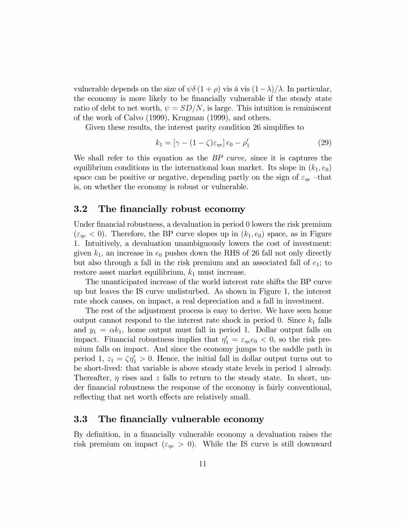
k1 = [γ − (1− ζ)εηe] e0 − ρ01 (29)

We shall refer to this equation as the BP curve, since it is captures theequilibrium conditions in the international loan market. Its slope in (k1, e0)space can be positive or negative, depending partly on the sign of εηe —thatis, on whether the economy is robust or vulnerable.

3.2 The financially robust economy

Under financial robustness, a devaluation in period 0 lowers the risk premium(εηe < 0). Therefore, the BP curve slopes up in (k1, e0) space, as in Figure1. Intuitively, a devaluation unambiguously lowers the cost of investment:given k1, an increase in e0 pushes down the RHS of 26 fall not only directlybut also through a fall in the risk premium and an associated fall of e1; torestore asset market equilibrium, k1 must increase.The unanticipated increase of the world interest rate shifts the BP curve

up but leaves the IS curve undisturbed. As shown in Figure 1, the interestrate shock causes, on impact, a real depreciation and a fall in investment.The rest of the adjustment process is easy to derive. We have seen home

output cannot respond to the interest rate shock in period 0. Since k1 fallsand y1 = αk1, home output must fall in period 1. Dollar output falls onimpact. Financial robustness implies that η01 = εηee0 < 0, so the risk pre-mium falls on impact. And since the economy jumps to the saddle path inperiod 1, z1 = ζη01 > 0. Hence, the initial fall in dollar output turns out tobe short-lived: that variable is above steady state levels in period 1 already.Thereafter, η rises and z falls to return to the steady state. In short, un-der financial robustness the response of the economy is fairly conventional,reflecting that net worth effects are relatively small.

3.3 The financially vulnerable economy

By definition, in a financially vulnerable economy a devaluation raises therisk premium on impact (εηe > 0). While the IS curve is still downward

11

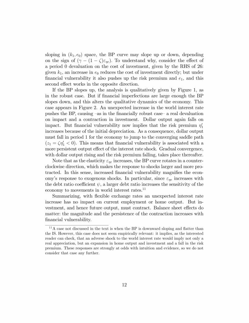
sloping in (k1, e0) space, the BP curve may slope up or down, dependingon the sign of (γ − (1 − ζ)εηe). To understand why, consider the effect ofa period 0 devaluation on the cost of investment, given by the RHS of 26:given k1, an increase in e0 reduces the cost of investment directly; but underfinancial vulnerability it also pushes up the risk premium and e1, and thissecond effect works in the opposite direction.If the BP slopes up, the analysis is qualitatively given by Figure 1, as

in the robust case. But if financial imperfections are large enough the BPslopes down, and this alters the qualitative dynamics of the economy. Thiscase appears in Figure 2. An unexpected increase in the world interest ratepushes the BP, causing —as in the financially robust case— a real devaluationon impact and a contraction in investment. Dollar output again falls onimpact. But financial vulnerability now implies that the risk premium η01increases because of the initial depreciation. As a consequence, dollar outputmust fall in period 1 for the economy to jump to the converging saddle path(z1 = ζη01 < 0). This means that financial vulnerability is associated with amore persistent output effect of the interest rate shock. Gradual convergence,with dollar output rising and the risk premium falling, takes place thereafter.Note that as the elasticity εηε increases, the BP curve rotates in a counter-

clockwise direction, which makes the response to shocks larger and more pro-tracted. In this sense, increased financial vulnerability magnifies the econ-omy’s response to exogenous shocks. In particular, since εηe increases withthe debt ratio coefficient ψ, a larger debt ratio increases the sensitivity of theeconomy to movements in world interest rates.11

Summarizing, with flexible exchange rates an unexpected interest rateincrease has no impact on current employment or home output. But in-vestment, and hence future output, must contract. Balance sheet effects domatter: the magnitude and the persistence of the contraction increases withfinancial vulnerability.

11A case not discussed in the text is when the BP is downward sloping and flatter thanthe IS. However, this case does not seem empirically relevant: it implies, as the interestedreader can check, that an adverse shock to the world interest rate would imply not only areal appreciation, but an expansion in home output and investment and a fall in the riskpremium. These responses are strongly at odds with intuition and evidence, so we do notconsider that case any further.

12

4 Fixed Exchange Rates

Focus now on a policy of fixed exchange rates, defined as a regime in whichthe monetary authority keeps the nominal exchange rate constant: st = 0 forall t. Again, we consider the effects of an unexpected and temporary increaseof the world real interest rate at time 0.With fixed exchange rates, real depreciations (appreciations) can only

be accomplished through deflation (inflation): et = −pt. Now, the Phillipscurve 21 yields

y0 =

µ1− α

α

¶p0 = −

µ1− α

α

¶e0, (30)

reflecting that a real devaluation is associated with unexpected deflation and,because nominal wages are fixed, a fall in home output on impact.The derivation of the IS schedule is the same as with flexible exchange

rates, except that y0 is no longer zero but given 30. Hence the IS is

y0 = −µ1− α

α

¶e0 = λk1 + (1− λγ)e0. (31)

This curve is still downward sloping, but flatter than under flexible exchangerates. This reflects the fact that a real devaluation requires price deflationand a fall in home output falls. To restore equilibrium in the home goodsmarket, investment must fall by more than under flexible exchange rates.The derivation of the BP curve is also the same as with flexible rates,

except that 17 now implies that the response of the risk premium to a deval-uation is

η01 = µα−1µψδ (1 + ρ)− 1− λ

λ

¶e0 = α−1εηee0. (32)

In words, the elasticity of the premium with respect to the initial real ex-change rate is the same as with flexible exchange rates, but scaled up byα−1. This reflects that, in addition to effects previously encountered, anunexpected devaluation is now associated with a fall in output and capitalincome, reducing net worth and pushing up the risk premium further. Theconsequence is that the BP curve is

k1 =£γ − (1− ζ)εηeα

−1¤ e0 − ρ01. (33)

This is the same as before, except that εηe is replaced by εηeα−1.

13

As with flexible rates, dynamic adjustment is easily described by the ISand BP curves. Under financial robustness, the IS curve slopes down and theBP curve slopes up as in the flexible rates case, although they are both flatter.This means that Figure 1 still captures the qualitative response to a shockto the world interest rate. But there is an important difference which doesnot appear in the figure: with fixed exchange rates, the period 0 devaluationis associated with price deflation and a fall in home output and domesticemployment.Since the IS and BP are both flatter, the increase in e0 is smaller than

with flexible rates, which is intuitive. Graphical analysis is less useful tocompare the changes in k1. However, it is easy enough to solve the IS andthe BP algebraically for k1 under both exchange rate regimes. One can showthat the fall in investment is greater under fixed rates.Under financial vulnerability, εηe > 0 and the BP may slope up or down.

If it slopes up, the analysis is similar to that under financial robustness,except that the BP curve is steeper under fixed exchange rates than withflexible rates, while the IS curve is still flatter under fixed rates. This meansthat the adjustment to an adverse interest rate shock requires an even deeperfall in investment under fixed rates.If financial imperfections are sufficiently large so that the BP has a neg-

ative slope, the responses of e0 and k1 are still shown qualitatively in Figure2,12 although both the IS and the BP are both flatter than under flexiblerates. This clearly implies that, in response to an interest rate shock, theincrease in e0 is smaller under fixed rates. But again this comes at the ex-pense of a fall in home output and employment on impact. Moreover, thefall in investment turns out to be greater with fixed rates, as can be checkedalgebraically.The conclusion is that, in response to a shock to the world interest rate,

the impact real devaluation is smaller under fixed rates than under flexiblerates. But the cost is that, under fixed rates, the devaluation requires pricedeflation, and hence an initial fall in home output that is absent under flexiblerates. We have also argued that the fall in investment is greater under fixedrates, which reflects the fact that the cost of capital is higher.

12For the same reasons as in the previous footnote, we ignore the case in which the BPis downward sloping but flatter than the IS.

14

5 On the Optimality of Flexible Rates

While our discussion has focused on the dynamics of the model under fixedand flexible exchange rates, these comparative dynamics do reflect a welfareranking. In fact, flexible rates are not only Pareto superior to fixed rates,but socially optimal. This is the point of this section.Note first that, in this model, entrepreneurial welfare does not depend on

monetary policy: entrepreneurial consumption in each period is a fractionof net worth in dollars, which is independent of monetary policy. It followsthat optimal monetary policy must maximize the welfare of the representativeworker. Note also that to analyze welfare one must consider not only one-time shocks, but stochastic equilibria under different policy regimes.The expected welfare of the representative worker in equilibrium is given

by −1©P∞

t=0 β£logCt − σ−1

σνLνt

¤ª, where β is the workers’ discount factor.

However, for any t, −1Lνt =−1 (t−1L

νt ) = 1, where the first equality follows

from the Law of Iterated Expectations, and the second equality from 10.Hence optimal policy maximizes expected discounted log consumption. Tak-ing logs in 4, 8, and 9 and simplifying yields

logCt = γ log Yt + (1− γ) logZt + log(1− α). (34)

Replacing in the preceding equation and recalling that dollar output is in-dependent of monetary policy, it follows that optimal policy maximizes theexpected discounted value of log output, −1(

P∞t=0 β log Yt).

Since the production function is Cobb Douglas, log Yt = α logKt + (1−α) logLt. Now, logK0 is given, while using 12 and iterating one shows thatlogKt equals γ(1− α)[logLt−1 + α logLt−2 + ...+ αt−1 logL0] + (γα)t logK0

plus a term that is independent of policy. Hence optimality requires themaximization of a linear combination of terms of the form −1 logLt, t =0, 1, ... But now 10 and a simple application of Jensen’s inequality imply thatflexible exchange rates maximize each those terms and, hence, are optimal.13

The intuition is that there are three key distortions affecting the economy:workers have some monopoly power, financial contracts are imperfect, andwages are rigid in pesos. Monetary policy cannot counteract the effects ofthe first two distortions, but it can undo the effects of nominal rigidity.

13Note −1 logLt = −1(logLνt )ν−1. This is the expectation, at t = −1, of a concavefunction of Lνt . Moreover, −1(Lνt ) = −1(t−1Lνt ) = 1, independently of monetary policy, sothe claim follows by Jensen’s inequality.

15

6 Final Remarks

The interaction of dollarized debts and net worth complicates an economy’sresponse to external shocks. Under financial vulnerability, a real depreciationraises the risk premium. But trying to contain real depreciation pushesdomestic output down, and this is also bad for the risk premium. The netresult here is that the behavior of the risk premium is independent of theexchange regime, contrary to the conjectures in much of the recent policyliterature.While the exact offset depends on special assumptions, there is a general

message here: depreciation has contradictory and possibly offsetting effectson firms’ balance sheets. Therefore, exchange rate policy is unlikely to havemuch impact on the risk premium, and financial imperfections need not ren-der fixed rates more stabilizing than flexible rates.For tractability, we imposed strong assumptions. Relaxing them is nec-

essary for arriving at a quantitative evaluation of the model. But we havereason to think that our main results would survive.14 For instance, allow-ing for incomplete capital depreciation should strengthen the desirability offloating. In the model, the price of capital in terms of home goods is anincreasing function of the real exchange rate. With incomplete depreciation,a real depreciation would raise the value of capital, thereby increasing networth. That would constitute an additional advantage of a flexible exchangerate.15

We took the denomination of foreign bonds as given, while in realityit is endogenous and may depend on exchange rate policy. But there isno accepted view of how the menu of assets is related to the exchange rateregime.16 Simply assuming that all liabilities are dollarized is plausible, giventhat essentially all lending to emerging markets is denominated in a fewcurrencies. Doing so stacks the deck against flexible exchange rates, so ourpolicy conclusions do not hinge on this assumption.

14The working paper version explores the case in which the investment good aggregatoris a general CES function. We show that this extension does not overturn the resultspresented here.15But allowing for incomplete depreciation would change the quantitative implications of

the model. Balance sheet effects would be much smaller, since they act through investment.We thank a referee for making this point.16See the recent work by Burnside, Eichenbaum and Rebelo (2001), Schneider and Tor-

nell (2004), Caballero and Krishnamurthy (2003), Jeanne (2001) and Chamon (2001).

16

References

[1] Aghion, Philippe; Bacchetta, Philippe and Banerjee, Abhijit. “A SimpleModel of Monetary Policy and Currency Crises.” European EconomicReview, May 2000 (Papers and Proceedings), 44(4-6), pp. 728-738.

[2] Bernanke, Ben and Gertler, Mark. “Agency Costs, Net Worth, and Busi-ness Fluctuations.” American Economic Review, March 1989, 79(1), pp.14-31.

[3] Bernanke, Ben; Gertler, Mark and Gilchrist, Simon. “The Financial Ac-celerator in a Quantitative Business Cycle Framework.” in J. Taylor andM. Woodford, eds., Handbook of Macroeconomics. Amsterdam: North-Holland, 1999, pp. 1341-1393.

[4] Burnside, Craig; Eichenbaum, Martin and Rebelo, Sergio. “Hedging andFinancial Fragility in Fixed Exchange Rate Regimes.” European Eco-nomic Review, 2001, 45(7), pp. 1151-1193.

[5] Caballero, Ricardo and Krishnamurthy, Arvind. “Excessive Dollar Debt:Financial Development and Underinsurance.” Journal of Finance, April2003, 58(2), pp. 867-893.

[6] Calvo, Guillermo. “Fixed vs. Flexible Exchange Rates: Preliminaries ofa Turn-of-Millennium Rematch.” Mimeo, University of Maryland, 1999.

[7] Calvo, Guillermo. “Capital Market and The Exchange Rate With Spe-cial Reference to the Dollarization Debate in Latin America.” Journalof Money, Credit and Banking, May 2001, 33(2), pp. 312-334.

[8] Calvo, Guillermo and Reinhart, Carmen. “Fear of Floating.” QuarterlyJournal of Economics, May 2002, 117(2), pp. 379-408.

[9] Céspedes, Luis F. “Credit Constraints and Macroeconomic Instabilityin a Small Open Economy.” Mimeo, NYU, April 2000.

[10] Chamon, Marcos. “Why Can’t Developing Countries Borrow in theirOwn Currencies?.” Mimeo, Harvard University, October 2001.

[11] Dixit, Avinash and Stiglitz, Joseph. “Monopolistic Competition andOptimum Product Diversity.” American Economic Review, June 1977,67(3), pp. 297-308.

17

[12] Hausmann, Ricardo; Panizza, Ugo and Stein, Ernesto. “Why Do Coun-tries Float the Way they Float?.” Working Paper No. 418, Inter-American Development Bank, May 2000.

[13] Jeanne, Olivier. “Why Do Emerging Economies Borrow in Foreign Cur-rency?.” Mimeo, International Monetary Fund, October 2001.

[14] Krugman, Paul. “Balance Sheets, the Transfer Problem and FinancialCrises.” in P. Isard, A. Razin and A. Rose, eds., International Financeand Financial Crises, Kluwer Academic Publishers, 1999.

[15] Lane, Philip. “The New Open-Economy Macroeconomics: A Survey.”Journal of International Economics, August 2001, 54(2), pp. 235-266.

[16] Obstfeld, Maurice and Rogoff, Kenneth. “New Directions for StochasticOpen Economy Models.” Journal of International Economics, February2000, 50(1), pp. 117-153.

[17] Schneider, Martin and Tornell Aaron. “Balance Sheets Effects, BailoutGuarantees and Financial Crises.” Review of Economic Studies, 2004(forthcoming).

[18] Williamson, Stephen. “Costly Monitoring, Loan Contracts, and Equi-librium Credit Rationing.” Quarterly Journal of Economics, February1987, 102(1), pp. 135-45.

[19] Woodford, Michael. Interest and Prices: Foundations of a Theory ofMonetary Policy, Princeton University Press, 2003.

18

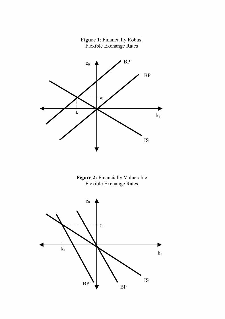
Figure 1: Financially RobustFlexible Exchange Rates

Figure 2: Financially VulnerableFlexible Exchange Rates

e0

k1

e0

k1

BP

BP`

IS

e0

k1

e0

k1

BPBP` IS

Appendix to "Balance Sheets and ExchangeRate Policy"

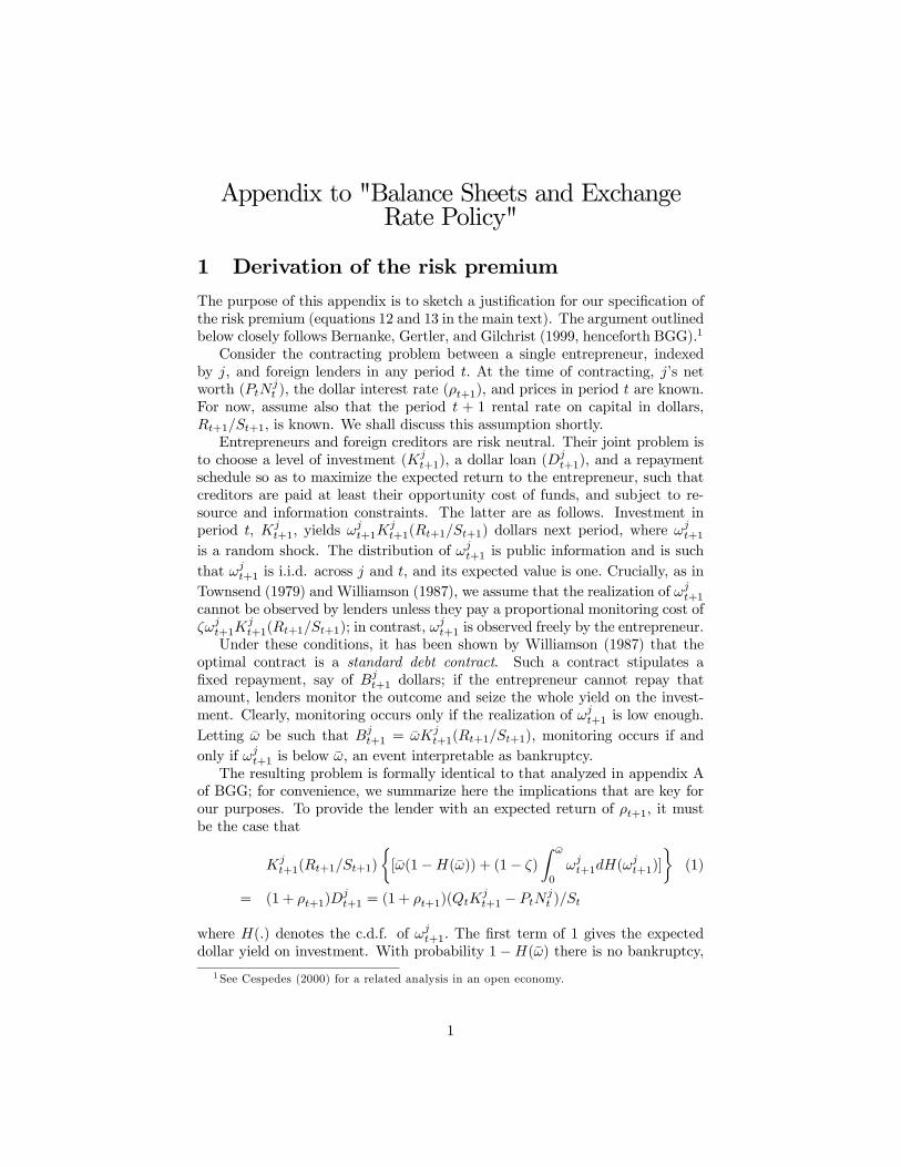
1 Derivation of the risk premium

The purpose of this appendix is to sketch a justification for our specification ofthe risk premium (equations 12 and 13 in the main text). The argument outlinedbelow closely follows Bernanke, Gertler, and Gilchrist (1999, henceforth BGG).1

Consider the contracting problem between a single entrepreneur, indexedby j, and foreign lenders in any period t. At the time of contracting, j’s networth (PtN

jt ), the dollar interest rate (ρt+1), and prices in period t are known.

For now, assume also that the period t + 1 rental rate on capital in dollars,Rt+1/St+1, is known. We shall discuss this assumption shortly.Entrepreneurs and foreign creditors are risk neutral. Their joint problem is

to choose a level of investment (Kjt+1), a dollar loan (D

jt+1), and a repayment

schedule so as to maximize the expected return to the entrepreneur, such thatcreditors are paid at least their opportunity cost of funds, and subject to re-source and information constraints. The latter are as follows. Investment inperiod t, Kj

t+1, yields ωjt+1K

jt+1(Rt+1/St+1) dollars next period, where ωjt+1

is a random shock. The distribution of ωjt+1 is public information and is suchthat ωjt+1 is i.i.d. across j and t, and its expected value is one. Crucially, as inTownsend (1979) and Williamson (1987), we assume that the realization of ωjt+1cannot be observed by lenders unless they pay a proportional monitoring cost ofζωjt+1K

jt+1(Rt+1/St+1); in contrast, ω

jt+1 is observed freely by the entrepreneur.

Under these conditions, it has been shown by Williamson (1987) that theoptimal contract is a standard debt contract. Such a contract stipulates afixed repayment, say of Bj

t+1 dollars; if the entrepreneur cannot repay thatamount, lenders monitor the outcome and seize the whole yield on the invest-ment. Clearly, monitoring occurs only if the realization of ωjt+1 is low enough.Letting ω be such that Bj

t+1 = ωKjt+1(Rt+1/St+1), monitoring occurs if and

only if ωjt+1 is below ω, an event interpretable as bankruptcy.The resulting problem is formally identical to that analyzed in appendix A

of BGG; for convenience, we summarize here the implications that are key forour purposes. To provide the lender with an expected return of ρt+1, it mustbe the case that

Kjt+1(Rt+1/St+1)

½[ω(1−H(ω)) + (1− ζ)

Z ω

0

ωjt+1dH(ωjt+1)]

¾(1)

= (1 + ρt+1)Djt+1 = (1 + ρt+1)(QtK

jt+1 − PtN

jt )/St

where H(.) denotes the c.d.f. of ωjt+1. The first term of 1 gives the expecteddollar yield on investment. With probability 1−H(ω) there is no bankruptcy,

1 See Cespedes (2000) for a related analysis in an open economy.

1

and lenders are repaid Bjt+1 = ωKj

t+1(Rt+1/St+1). With probability H(ω), theentrepreneur goes bankrupt, and lenders are repaid whatever is left after mon-itoring costs; this is the term (1 − ζ)Kj

t+1(Rt+1/St+1)R ω0ωjt+1dH(ω

jt+1). The

first equality in 1 gives the opportunity cost of the loan Djt+1. The second equal-

ity takes into account that the loan must equal the value of investment minusthe entrepreneur’s net worth.The optimal contract maximizes the entrepreneur’s utility

[

Z ∞ω

ωjt+1dH(ωjt+1)− ω(1−H(ω))]Rt+1K

jt+1 (2)

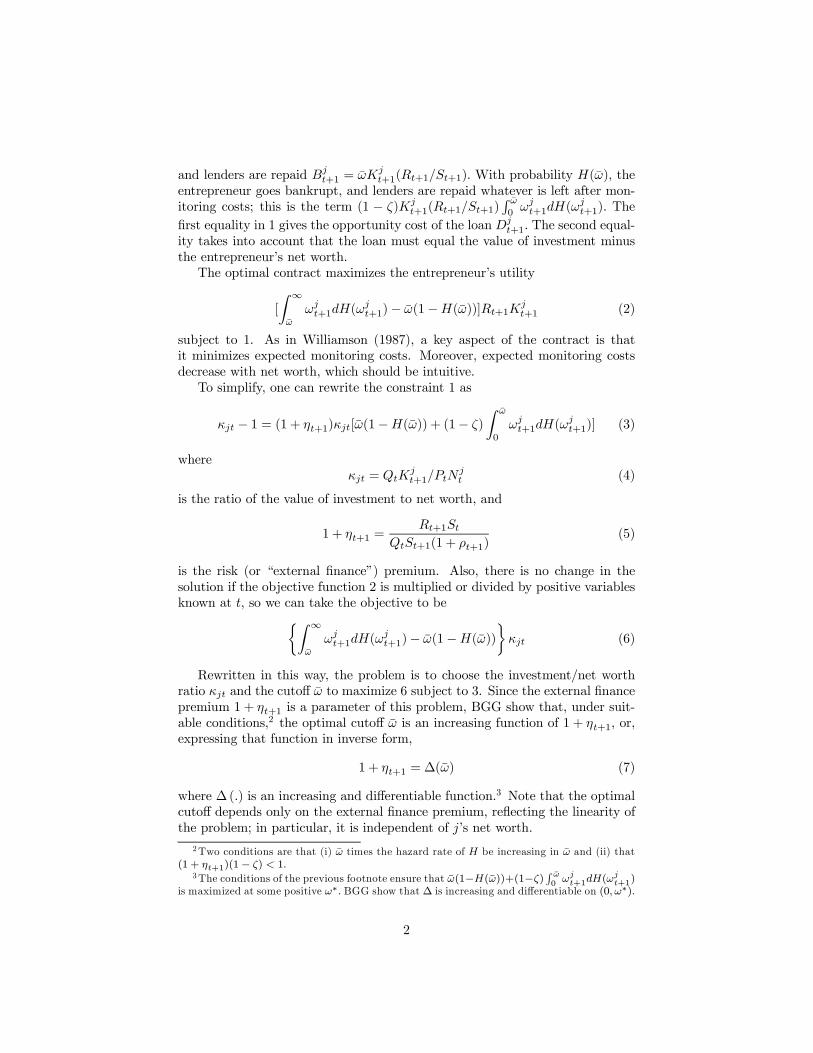
subject to 1. As in Williamson (1987), a key aspect of the contract is thatit minimizes expected monitoring costs. Moreover, expected monitoring costsdecrease with net worth, which should be intuitive.To simplify, one can rewrite the constraint 1 as

κjt − 1 = (1 + ηt+1)κjt[ω(1−H(ω)) + (1− ζ)

Z ω

0

ωjt+1dH(ωjt+1)] (3)

whereκjt = QtK

jt+1/PtN

jt (4)

is the ratio of the value of investment to net worth, and

1 + ηt+1 =Rt+1St

QtSt+1(1 + ρt+1)(5)

is the risk (or “external finance”) premium. Also, there is no change in thesolution if the objective function 2 is multiplied or divided by positive variablesknown at t, so we can take the objective to be½Z ∞

ω

ωjt+1dH(ωjt+1)− ω(1−H(ω))

¾κjt (6)

Rewritten in this way, the problem is to choose the investment/net worthratio κjt and the cutoff ω to maximize 6 subject to 3. Since the external financepremium 1 + ηt+1 is a parameter of this problem, BGG show that, under suit-able conditions,2 the optimal cutoff ω is an increasing function of 1 + ηt+1, or,expressing that function in inverse form,

1 + ηt+1 = ∆(ω) (7)

where ∆ (.) is an increasing and differentiable function.3 Note that the optimalcutoff depends only on the external finance premium, reflecting the linearity ofthe problem; in particular, it is independent of j’s net worth.

2Two conditions are that (i) ω times the hazard rate of H be increasing in ω and (ii) that(1 + ηt+1)(1− ζ) < 1.

3The conditions of the previous footnote ensure that ω(1−H(ω))+(1−ζ) R ω0 ωjt+1dH(ωjt+1)

is maximized at some positive ω∗. BGG show that ∆ is increasing and differentiable on (0, ω∗).

2

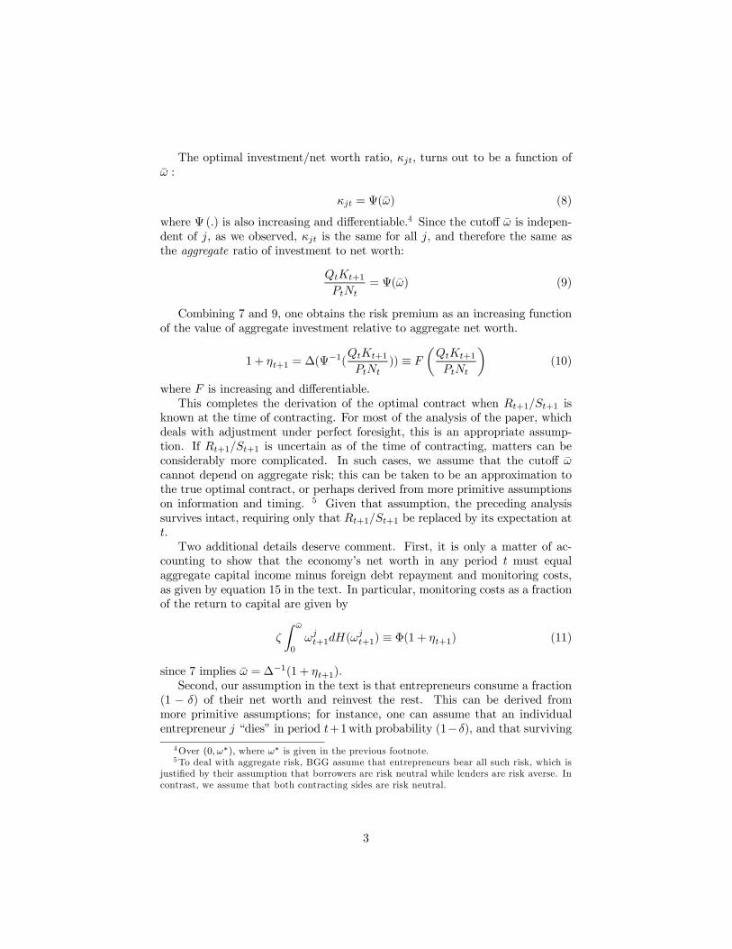
The optimal investment/net worth ratio, κjt, turns out to be a function ofω :

κjt = Ψ(ω) (8)

where Ψ (.) is also increasing and differentiable.4 Since the cutoff ω is indepen-dent of j, as we observed, κjt is the same for all j, and therefore the same asthe aggregate ratio of investment to net worth:

QtKt+1

PtNt= Ψ(ω) (9)

Combining 7 and 9, one obtains the risk premium as an increasing functionof the value of aggregate investment relative to aggregate net worth.

1 + ηt+1 = ∆(Ψ−1(

QtKt+1

PtNt)) ≡ F

µQtKt+1

PtNt

¶(10)

where F is increasing and differentiable.This completes the derivation of the optimal contract when Rt+1/St+1 is

known at the time of contracting. For most of the analysis of the paper, whichdeals with adjustment under perfect foresight, this is an appropriate assump-tion. If Rt+1/St+1 is uncertain as of the time of contracting, matters can beconsiderably more complicated. In such cases, we assume that the cutoff ωcannot depend on aggregate risk; this can be taken to be an approximation tothe true optimal contract, or perhaps derived from more primitive assumptionson information and timing. 5 Given that assumption, the preceding analysissurvives intact, requiring only that Rt+1/St+1 be replaced by its expectation att.Two additional details deserve comment. First, it is only a matter of ac-

counting to show that the economy’s net worth in any period t must equalaggregate capital income minus foreign debt repayment and monitoring costs,as given by equation 15 in the text. In particular, monitoring costs as a fractionof the return to capital are given by

ζ

Z ω

0

ωjt+1dH(ωjt+1) ≡ Φ(1 + ηt+1) (11)

since 7 implies ω = ∆−1(1 + ηt+1).Second, our assumption in the text is that entrepreneurs consume a fraction

(1 − δ) of their net worth and reinvest the rest. This can be derived frommore primitive assumptions; for instance, one can assume that an individualentrepreneur j “dies” in period t+1with probability (1−δ), and that surviving

4Over (0, ω∗), where ω∗ is given in the previous footnote.5To deal with aggregate risk, BGG assume that entrepreneurs bear all such risk, which is

justified by their assumption that borrowers are risk neutral while lenders are risk averse. Incontrast, we assume that both contracting sides are risk neutral.

3

entrepreneurs are patient enough so that they choose not to consume theirwealth until death.6

2 Steady State and Linear Approximation

Here we sketch the proof of the existence and uniqueness of a non-stochasticsteady state, describe our linear approximation to the equilibrium system, anddiscuss non-stochastic dynamics.One can show that, in steady state, the Lagrange multiplier associated with 3

must equal the inverse of δ(1+ρ). The analysis of BGG shows that the Lagrangemultiplier is an increasing function of ω, which goes to one as ω goes to zeroand to infinity as ω goes to ω∗, where ω∗ > 0 is defined in their footnote 2.So, provided that 0 < δ(1 + ρ) < 1 there is a unique, strictly positive, steadystate solution for ω, with which one can pin down the values of η and QK

N atthe steady state.Now we need to solve for the remaining variables, whose steady state levels

are given by:

Y = AKα (12)

Q = S1−γ (13)

αY

QK= (1 + ρ)(1 + η) (14)

N + SD = QK (15)

Y = γ[(1− α)Y +QK] + SX (16)

Using 12 and 13 into 16 we obtain

(1− γ(1− α))Y − γS1−γ

A1/αY 1/α − SX = 0 (17)

Now, using 12 and 13 into 14 we obtain

S1−γY1−αα = α

A1/α

(1 + ρ)(1 + η)(18)

which is a hyperbola in (Y, S) space. Using 18 in 17 we obtain∙1− γ(1− α)− αγ

(1 + ρ)(1 + η)

¸Y = SX (19)

6To keep the number of entrepreneurs constant, one can assume that each dead en-trepreneur is replaced by a newborn one. A minor problem arises since new entrepreneursmust have some initial net worth to be able to borrow. This can be remedied by assuming thatnew entrepreneurs are born with an exogenous and arbitrarily small endowment, or that theyhave a small endowment of labor (as in Carlstrom and Fuerst 1998). The effects of choosingeither assumption would be negligible, and so we ignore this issue in the text.

4

Given that 1− γ(1− α)− αγ(1+ρ)(1+η) = (1− γ) + (γα− αγ

(1+ρ)(1+η)) > 0, this isa ray from the origin in (Y, S) space. The steady state values of Y and S mustsolve 18 and 19. Clearly, there is a unique positive solution. With this result inhand, it is simple to solve for the steady state values of K and Q using 12 and13.Log linearizing the equilibrium equations around the steady state just found,

we obtain a system that includes, whether wages are flexible or sticky, equations22, 23, and 24 in the text, the linearized version of the interest parity condition12:

tyt+1 − (qt − pt)− kt+1 = ρ0t+1 + η0t+1 +t (st+1 − pt+1)− (st − pt) (20)

and the following equation for the risk premium:

η0t+1 = φη0t + µ (qt − pt + kt+1 − yt) (21)

+µδ (1 + ρ)ψ [(st − pt − t−1(st − pt))− (yt − t−1yt)]

Here, λ = γQKγQK+SX = αγ

(1−γ+αγ)(1+ρ)(1+η) < 1, µ =F 0(.)F (.)

QKN , and φ =

δ (1 + ρ) (1 − µψ) + µ {δ (1 + ρ) (1 + ψ) η + δ (1 + ρ)− 1}³

υε∆

´where υ is

the elasticity ofR ω0 ωjt+1dH(ω

jt+1) with respect to ω and ε∆ is the elasticity of

the ∆ function in 10. Now 17 follows from 21 after using 22 to eliminate theterm (kt+1 + qt − pt) and recalling that the real exchange rate et equals st− pt.The calculation of the saddle-path zt = ζη0t is straightforward. Without

uncertainty, 17 and 18 can be written in matrix form as∙zt+1η0t+1

¸= Φ

∙ztη0t

¸(22)

We assume that the roots of Φ are real and that a saddle-path exists. Existenceof a saddle-path requires the two roots to be on opposite sides of the unitcircle; a sufficient condition is that φ < 1 + µ. The roots of Φ are real if[(1− λ) (1 + µ) + (1 + φ)λ]

2 > 4φλ. Both sufficient conditions must hold, inparticular, if µ is small enough — that is, if financial imperfections are not toostringent.Standard techniques now yield the saddle-path coefficient ζ = λ

µ(1−λ) {ξ2 − φ},where ξ2 is the smaller eigenvalue of Φ. The term in curly brackets is negative,and hence ζ < 0 as stated in the text.

3 Optimality of Flexible Rates

Here we show the validity of an assertion in section 5. For all t, it is easy toshow that taking logs in 12 one obtains

logKt+1 = logα+ γ logYt + logt Zt+1− γ logZt − log(1 + ρt+1)− log(1 + ηt+1)

5

SologKt+1 = γ[α logKt + (1− α) logLt] + Λt

where the term Λt = logα+log tZt+1−γ logZt− log(1+ρt+1)− log(1+ηt+1) isindependent of monetary or exchange rate policy. Using the previous expressionlagged one period to replace logKt, and continuing back to period 0, we get

logKt+1 = γ(1− α) logLt + γα[γ[α logKt−1 + (1− α) logLt−1] + Λt−1] + Λt= γ(1− α)[logLt + α logLt−1] + (γα)2 logKt−1 + Λt + γαΛt−1= ...

= γ(1− α)[logLt + α logLt−1 + ...+ αt logL0] + (γα)t+1 logK0 +Υt+1

where Υt+1 is, again, independent of policy, as claimed.

6