Bal Harbour Mitigation Artificial Reef Monitoring … Harbour Mitigation Artificial Reef Monitoring...

Bal Harbour Mitigation

Artificial Reef Monitoring Program

Year 12 1999 – 2011

Progress Report and Summary

Submitted to the State of Florida Department of Environmental Protection in partial fulfillment

of the

Bal Harbour Consent Order - OGC Case No. 94-2842

Miami-Dade County

Permitting, Environment and Regulatory Affairs Melissa P. Sathe, Sara E. Thanner, and Stephen M. Blair

Y12 Bal Harbour Mitigation Project Report

2

INTRODUCTION

This report provides information from an ongoing study of an artificial reef that was constructed

as mitigation for impacts to natural reefs. A 20-year monitoring program was developed to

assess the efficacy of the project as mitigation for natural reef impacts through the evaluation of

colonization and succession of assemblages on two types of artificial reef materials, as well as

comparisons to the adjacent natural reefs. The first five years of the project has been previously

documented (Thanner et al., 2006). Years 6 through 9 were documented in progress reports

submitted in April of 2007 (Y6 and Y7) and April of 2009 (Y8 and Y9). Year 10 was

documented in a Bi-Annual report submitted in April 2010. This report focuses on the

monitoring results of Year 12 with a summary of the monitoring data to date.

PROJECT BACKGROUND

During the summer of 1990, a beach renourishment project was constructed in which

approximately 400,000 cubic yards of sand from an offshore borrow area were deposited to

renourish 1.4 km of shoreline in the town of Bal Harbour (Miami-Dade County, Florida).

During the construction of this project, excessive sedimentation was discovered over 100,000 m2

of reef adjacent to the borrow area (Blair et al. 1990). As a result, the Florida Department of

Environmental Protection (FDEP) conducted an impact assessment including a ‗lost service‘

evaluation of the impacted reef (Florida Department of Environmental Protection, 1994), and

determined that 2938 m2 of artificial reef material would be required as mitigation.

Subsequently, a consent order (FDEP OGC File No. 94-2842) was signed in December of 1994.

The requirements of the consent order included the construction and deployment of the 2938 m2

of artificial reef material as mitigation, as well as a long-term biological monitoring plan to

evaluate the success of the mitigation.

From Miami-Dade County north to St. Lucie Inlet in Martin County, the offshore reef system is

comprised of a parallel series of low-relief carbonate ridges with a moderate amount of cryptic

habitat. These natural reefs provide habitat for, and support a diverse assemblage of benthic and

fish communities (Blair and Flynn, 1989; Goldberg, 1973; Lindeman, 1997; Moyer et al., 2003).

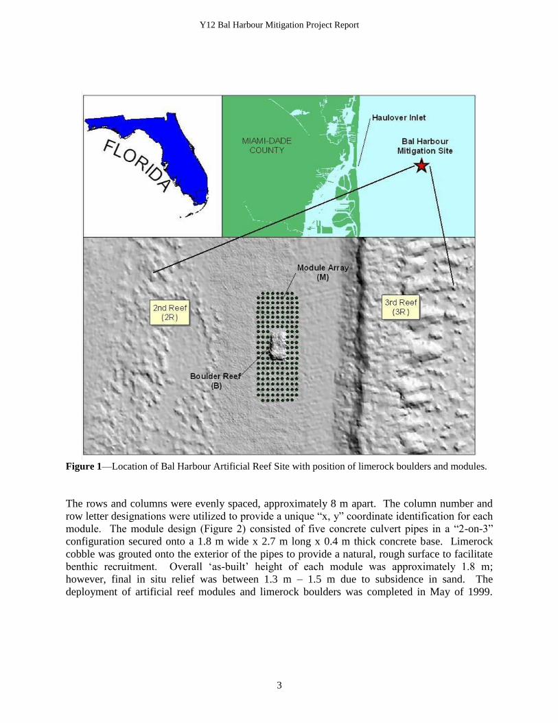
The artificial reef (mitigation) was constructed in the sand plain between two of the parallel reef

tracts. These parallel tracts are locally known as ―Second Reef‖ (2R) and ―Third Reef‖ (3R)

(Figure 1). The natural reef study areas on 2R and 3R adjacent to the artificial reef site were not

impacted in the Bal Harbour Renourishment Project. This artificial reef site is approximately 3.1

km offshore of Baker‘s Haulover Inlet, Miami-Dade County, at a depth of 20 m.

The design of the artificial reef included two major components: a multi-layer aggregation of

natural limestone boulders surrounded by an array of prefabricated concrete modules. The

boulder reef was constructed with approximately 8,000 tons of 0.9 m – 1.5 m diameter limerock

boulders arranged in a north/south (N/S) rectangular configuration (approximately 46 m by 23

m), with a vertical relief ranging from 2.5 m – 3.5 m. A matrix of 176 prefabricated concrete

and limerock modules was arranged in nine numbered columns (N/S) and 22 lettered rows (E/W)

surrounding the rectangular boulder area (Figure 1). The artificial reef is located between

Latitudes 25° 54.080‘ and 25° 54.180‘ North, and Longitudes 80° 05.365‘ and 80° 05.405‘ West.


3

Figure 1—Location of Bal Harbour Artificial Reef Site with position of limerock boulders and modules.

The rows and columns were evenly spaced, approximately 8 m apart. The column number and

row letter designations were utilized to provide a unique ―x, y‖ coordinate identification for each

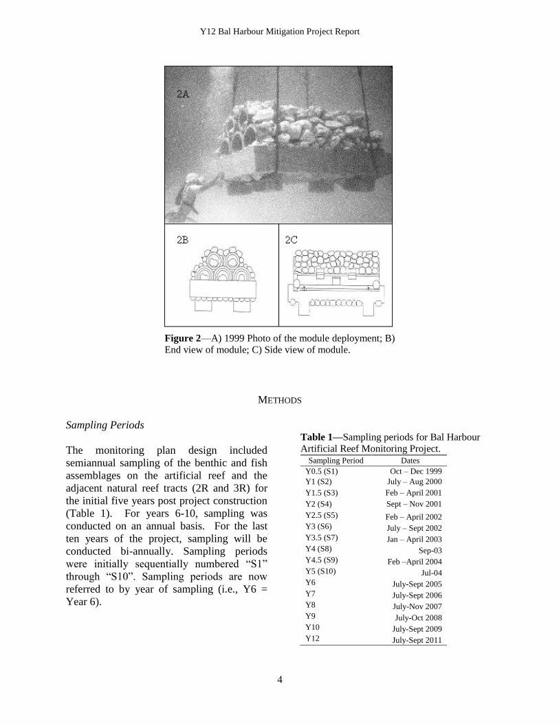
module. The module design (Figure 2) consisted of five concrete culvert pipes in a ―2-on-3‖

configuration secured onto a 1.8 m wide x 2.7 m long x 0.4 m thick concrete base. Limerock

cobble was grouted onto the exterior of the pipes to provide a natural, rough surface to facilitate

benthic recruitment. Overall ‗as-built‘ height of each module was approximately 1.8 m;

however, final in situ relief was between 1.3 m – 1.5 m due to subsidence in sand. The

deployment of artificial reef modules and limerock boulders was completed in May of 1999.


4

Figure 2—A) 1999 Photo of the module deployment; B)

End view of module; C) Side view of module.

METHODS

Sampling Periods

The monitoring plan design included

semiannual sampling of the benthic and fish

assemblages on the artificial reef and the

adjacent natural reef tracts (2R and 3R) for

the initial five years post project construction

(Table 1). For years 6-10, sampling was

conducted on an annual basis. For the last

ten years of the project, sampling will be

conducted bi-annually. Sampling periods

were initially sequentially numbered ―S1‖

through ―S10‖. Sampling periods are now

referred to by year of sampling (i.e., Y6 =

Year 6).

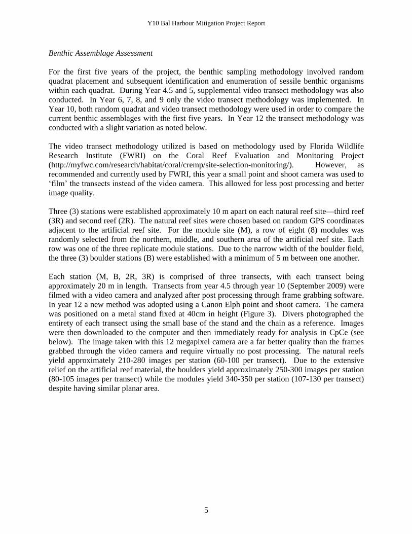
Table 1—Sampling periods for Bal Harbour

Artificial Reef Monitoring Project. Sampling Period Dates

Y0.5 (S1) Oct – Dec 1999

Y1 (S2) July – Aug 2000

Y1.5 (S3) Feb – April 2001

Y2 (S4) Sept – Nov 2001

Y2.5 (S5) Feb – April 2002

Y3 (S6) July – Sept 2002

Y3.5 (S7) Jan – April 2003

Y4 (S8) Sep-03

Y4.5 (S9) Feb –April 2004

Y5 (S10) Jul-04

Y6 July-Sept 2005

Y7 July-Sept 2006

Y8 July-Nov 2007

Y9 July-Oct 2008

Y10 July-Sept 2009

Y12 July-Sept 2011


5

Benthic Assemblage Assessment

For the first five years of the project, the benthic sampling methodology involved random

quadrat placement and subsequent identification and enumeration of sessile benthic organisms

within each quadrat. During Year 4.5 and 5, supplemental video transect methodology was also

conducted. In Year 6, 7, 8, and 9 only the video transect methodology was implemented. In

Year 10, both random quadrat and video transect methodology were used in order to compare the

current benthic assemblages with the first five years. In Year 12 the transect methodology was

conducted with a slight variation as noted below.

The video transect methodology utilized is based on methodology used by Florida Wildlife

Research Institute (FWRI) on the Coral Reef Evaluation and Monitoring Project

(http://myfwc.com/research/habitat/coral/cremp/site-selection-monitoring/). However, as

recommended and currently used by FWRI, this year a small point and shoot camera was used to

‗film‘ the transects instead of the video camera. This allowed for less post processing and better

image quality.

Three (3) stations were established approximately 10 m apart on each natural reef site—third reef

(3R) and second reef (2R). The natural reef sites were chosen based on random GPS coordinates

adjacent to the artificial reef site. For the module site (M), a row of eight (8) modules was

randomly selected from the northern, middle, and southern area of the artificial reef site. Each

row was one of the three replicate module stations. Due to the narrow width of the boulder field,

the three (3) boulder stations (B) were established with a minimum of 5 m between one another.

Each station (M, B, 2R, 3R) is comprised of three transects, with each transect being

approximately 20 m in length. Transects from year 4.5 through year 10 (September 2009) were

filmed with a video camera and analyzed after post processing through frame grabbing software.

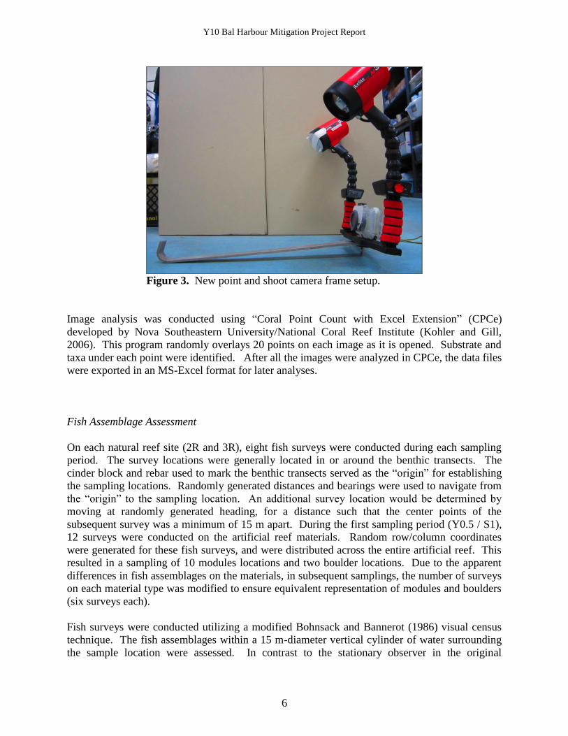
In year 12 a new method was adopted using a Canon Elph point and shoot camera. The camera

was positioned on a metal stand fixed at 40cm in height (Figure 3). Divers photographed the

entirety of each transect using the small base of the stand and the chain as a reference. Images

were then downloaded to the computer and then immediately ready for analysis in CpCe (see

below). The image taken with this 12 megapixel camera are a far better quality than the frames

grabbed through the video camera and require virtually no post processing. The natural reefs

yield approximately 210-280 images per station (60-100 per transect). Due to the extensive

relief on the artificial reef material, the boulders yield approximately 250-300 images per station

(80-105 images per transect) while the modules yield 340-350 per station (107-130 per transect)

despite having similar planar area.


6

Figure 3. New point and shoot camera frame setup.

Image analysis was conducted using ―Coral Point Count with Excel Extension‖ (CPCe)

developed by Nova Southeastern University/National Coral Reef Institute (Kohler and Gill,

2006). This program randomly overlays 20 points on each image as it is opened. Substrate and

taxa under each point were identified. After all the images were analyzed in CPCe, the data files

were exported in an MS-Excel format for later analyses.

Fish Assemblage Assessment

On each natural reef site (2R and 3R), eight fish surveys were conducted during each sampling

period. The survey locations were generally located in or around the benthic transects. The

cinder block and rebar used to mark the benthic transects served as the ―origin‖ for establishing

the sampling locations. Randomly generated distances and bearings were used to navigate from

the ―origin‖ to the sampling location. An additional survey location would be determined by

moving at randomly generated heading, for a distance such that the center points of the

subsequent survey was a minimum of 15 m apart. During the first sampling period (Y0.5 / S1),

12 surveys were conducted on the artificial reef materials. Random row/column coordinates

were generated for these fish surveys, and were distributed across the entire artificial reef. This

resulted in a sampling of 10 modules locations and two boulder locations. Due to the apparent

differences in fish assemblages on the materials, in subsequent samplings, the number of surveys

on each material type was modified to ensure equivalent representation of modules and boulders

(six surveys each).

Fish surveys were conducted utilizing a modified Bohnsack and Bannerot (1986) visual census

technique. The fish assemblages within a 15 m-diameter vertical cylinder of water surrounding

the sample location were assessed. In contrast to the stationary observer in the original


7

Bohnsack-Bannerot method, the diver swam two slow concentric circles during the first five

minutes of the survey, recording all species present within the cylinder. The first rotation was

made around the perimeter with minimal disturbance to the species present within the cylinder.

A second rotation was made at closer range to identify smaller, cryptic species that might

otherwise be missed. For the remainder of the survey, the diver continued this rotational pattern

enumerating and estimating the minimum, maximum, and mean size (in cm) of each fish species

recorded during the initial five minutes of the survey. Species observed after the initial five

minutes were also recorded. Additionally, station information, including habitat features and

sampling conditions, was recorded.

Although comprehensive fish survey datasets include all species observed and recorded, fish

assemblage analyses for this report were limited to those species characterized as the ―resident‖

species or guild (Bohnsack et al. 1994). Resident species tend to remain at one site and are often

observed on one or more consecutive surveys. Other classifications such as ―visitors‖ (only use

the habitat for temporary shelter or feeding) and ―transient‖ (roam over a wide area and appear

not to react to the reef presence) were omitted from analysis.

Statistical Analysis

The focus of this monitoring program was to document the changes in communities over time

(especially on the new artificial reef materials) and determine to what extent the communities on

the artificial reefs are similar to those of adjacent natural reefs. To achieve that goal, a

combination of assessment methods, utilization of similarity indices, and clustering with multi-

parameter scaling metrics were deemed appropriate for this evaluation. Multiple software

applications were used to summarize and analyze the benthic and fish population data.

Microsoft Excel was used to calculate summary statistics, graph results, and evaluate trends of

the data and indices. ―Primer-5 for Windows ‖ (Primer-E, 2002) multivariate statistical

software was used to calculate diversity and evenness indices, Bray-Curtis similarity indices

(Bray and Curtis, 1957), ordination clustering of the similarity data using non-metric

multidimensional scaling (MDS) procedures, and similarity percentage breakdowns (SIMPER).

The Shannon Diversity Index (H‘) was calculated as it incorporates species richness (S) as well

as the relative abundances of species. H‘ falls to zero when all the individuals in a population

sample belong to the same species and increases as the number of species increases. Relative

numbers of individuals of each species also affects the value of H‘. If only a small portion of

species in the sample account for most of the individuals, the value of H‘ will be lower than if all

the individuals were distributed evenly among all the species. Pielou‘s Evenness measure (J)

was also calculated because it expresses how evenly the individuals are distributed among the

different species. Higher values of J indicate the more evenly the individuals are spread among

the different species. Bray-Curtis Similarity indices were calculated once the data was fourth-

root transformed in order to reduce the weight of the common species and incorporate the

importance of both the intermediate and rare species (Field et. al 1982; Clark and Warwick

1994). The non-metric MDS analysis (Kruskal and Wish, 1978) generated a Shepard diagram

(graphical representation of the association of the groups analyzed), based on the calculated

Bray-Curtis indices. The MDS analysis generates a ―stress value‖ for each plot, which indicates

the level of difficulty in representing the similarity relationships for all samples into a two-

dimensional space. Clarke and Warwick (1994) state that a stress value ≤ 0.05 indicates a plot


8

with excellent representation and minimal chance of misinterpretation, values from 0.05 to 0.10

correspond to a good ordination with slight chance of misinterpretation, values from 0.10 to 0.20

indicate a potentially useful plot, but have a greater chance of misinterpretation, and values

between 0.20 and 0.30 are considered acceptable although conclusions should be crosschecked

with other statistical measures. Plots associated with stress levels ≥0.30 represent a more or less

arbitrary arrangement. SIMPER analysis produces an average dissimilarity between samples and

provides the percent contribution of each species to this dissimilarity.

RESULTS

Benthic Assemblages

This report summarizes the results from Y8-Y12 with the main focus being on the results from

the Y12 monitoring through the evaluation of the relative percent cover of benthic groups with

comparisons to previous year‘s results.

1. Assemblages on Natural Reefs

The benthic community components on the natural reefs showed consistency in the number of

species and lowest possible taxonomic group as well as the relative percent cover of benthic taxa

throughout the study period (Tables 2, 3). The algal group was the most abundant benthic

organisms on the natural reefs. Porifera and octocorallia continue to be the next most abundant

type benthic organisms on both 2R and 3R in terms of percent cover.

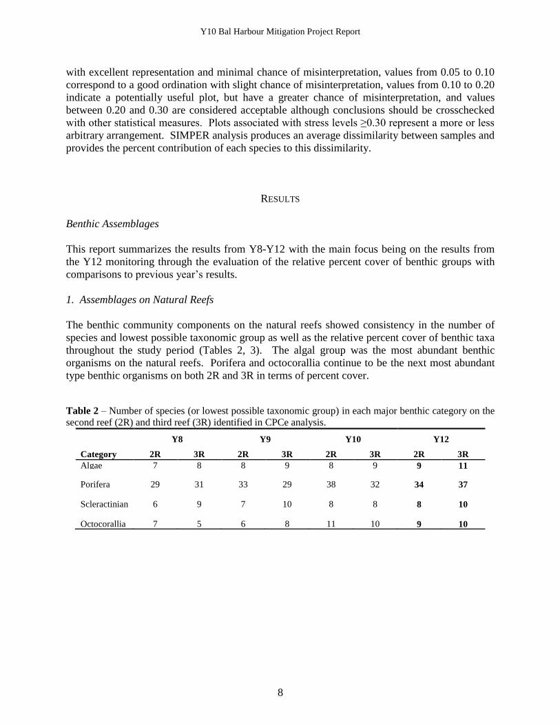
Table 2 – Number of species (or lowest possible taxonomic group) in each major benthic category on the

second reef (2R) and third reef (3R) identified in CPCe analysis.

Y8 Y9 Y10 Y12

Category 2R 3R 2R 3R 2R 3R 2R 3R

Algae 7 8 8 9 8 9 9 11

Porifera 29 31 33 29 38 32 34 37

Scleractinian 6 9 7 10 8 8 8 10

Octocorallia 7 5 6 8 11 10 9 10


9

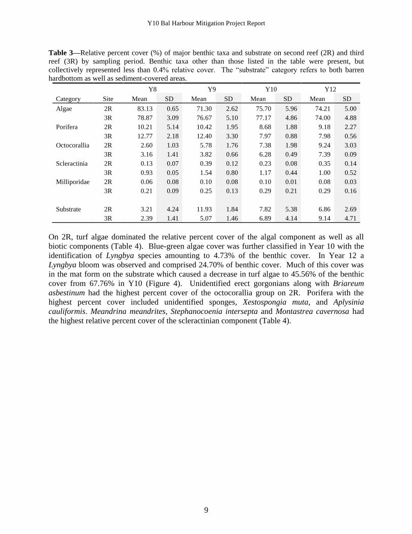
Table 3—Relative percent cover (%) of major benthic taxa and substrate on second reef (2R) and third

reef (3R) by sampling period. Benthic taxa other than those listed in the table were present, but

collectively represented less than 0.4% relative cover. The ―substrate‖ category refers to both barren

hardbottom as well as sediment-covered areas.

Y8 Y9 Y10 Y12

Category Site Mean SD Mean SD Mean SD Mean SD

Algae 2R 83.13 0.65 71.30 2.62 75.70 5.96 74.21 5.00

3R 78.87 3.09 76.67 5.10 77.17 4.86 74.00 4.88

Porifera 2R 10.21 5.14 10.42 1.95 8.68 1.88 9.18 2.27

3R 12.77 2.18 12.40 3.30 7.97 0.88 7.98 0.56

Octocorallia 2R 2.60 1.03 5.78 1.76 7.38 1.98 9.24 3.03

3R 3.16 1.41 3.82 0.66 6.28 0.49 7.39 0.09

Scleractinia 2R 0.13 0.07 0.39 0.12 0.23 0.08 0.35 0.14

3R 0.93 0.05 1.54 0.80 1.17 0.44 1.00 0.52

Milliporidae 2R 0.06 0.08 0.10 0.08 0.10 0.01 0.08 0.03

3R 0.21 0.09 0.25 0.13 0.29 0.21 0.29 0.16

Substrate 2R 3.21 4.24 11.93 1.84 7.82 5.38 6.86 2.69

3R 2.39 1.41 5.07 1.46 6.89 4.14 9.14 4.71

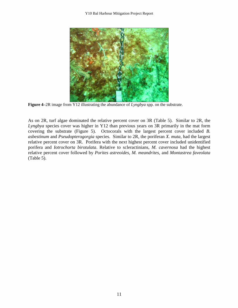
On 2R, turf algae dominated the relative percent cover of the algal component as well as all

biotic components (Table 4). Blue-green algae cover was further classified in Year 10 with the

identification of Lyngbya species amounting to 4.73% of the benthic cover. In Year 12 a

Lyngbya bloom was observed and comprised 24.70% of benthic cover. Much of this cover was

in the mat form on the substrate which caused a decrease in turf algae to 45.56% of the benthic

cover from 67.76% in Y10 (Figure 4). Unidentified erect gorgonians along with Briareum

asbestinum had the highest percent cover of the octocorallia group on 2R. Porifera with the

highest percent cover included unidentified sponges, Xestospongia muta, and Aplysinia

cauliformis. Meandrina meandrites, Stephanocoenia intersepta and Montastrea cavernosa had

the highest relative percent cover of the scleractinian component (Table 4).


10

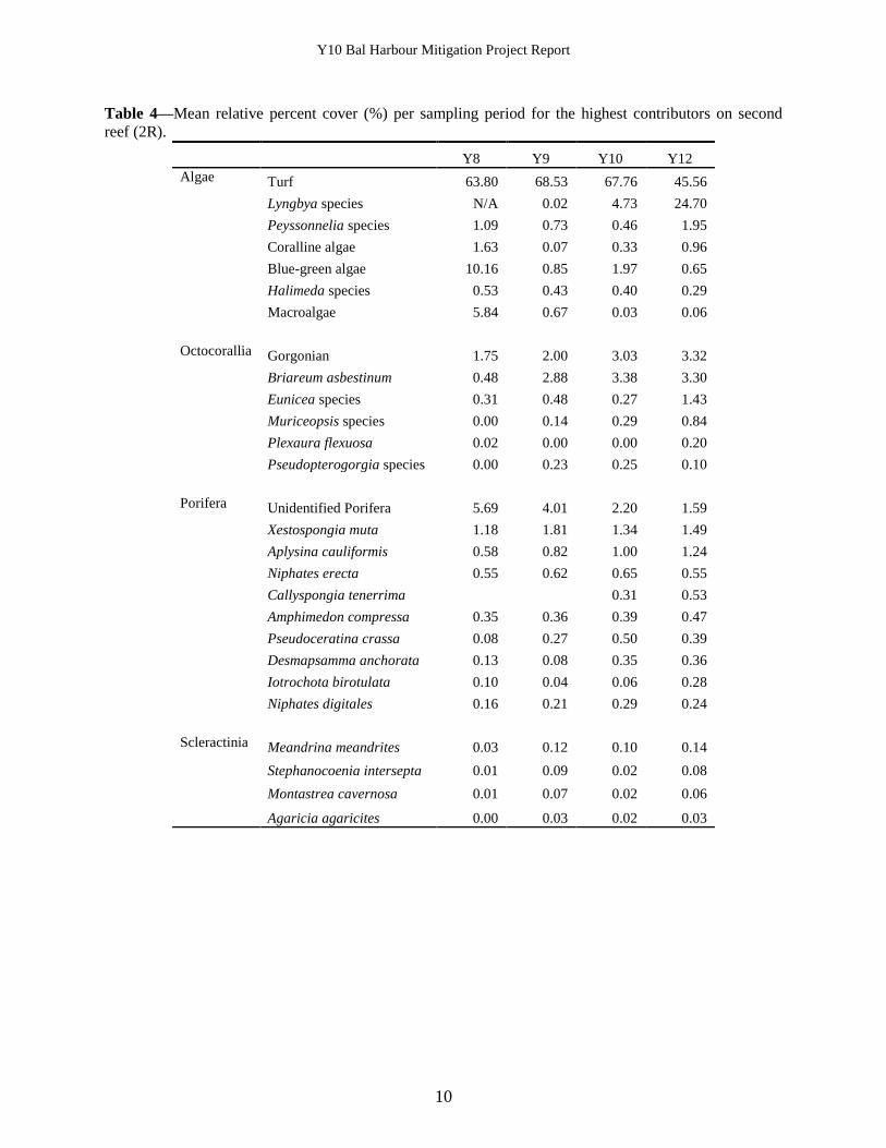
Table 4—Mean relative percent cover (%) per sampling period for the highest contributors on second

reef (2R).

Y8 Y9 Y10 Y12

Algae Turf 63.80 68.53 67.76 45.56

Lyngbya species N/A 0.02 4.73 24.70

Peyssonnelia species 1.09 0.73 0.46 1.95

Coralline algae 1.63 0.07 0.33 0.96

Blue-green algae 10.16 0.85 1.97 0.65

Halimeda species 0.53 0.43 0.40 0.29

Macroalgae 5.84 0.67 0.03 0.06

Octocorallia Gorgonian 1.75 2.00 3.03 3.32

Briareum asbestinum 0.48 2.88 3.38 3.30

Eunicea species 0.31 0.48 0.27 1.43

Muriceopsis species 0.00 0.14 0.29 0.84

Plexaura flexuosa 0.02 0.00 0.00 0.20

Pseudopterogorgia species 0.00 0.23 0.25 0.10

Porifera Unidentified Porifera 5.69 4.01 2.20 1.59

Xestospongia muta 1.18 1.81 1.34 1.49

Aplysina cauliformis 0.58 0.82 1.00 1.24

Niphates erecta 0.55 0.62 0.65 0.55

Callyspongia tenerrima

0.31 0.53

Amphimedon compressa 0.35 0.36 0.39 0.47

Pseudoceratina crassa 0.08 0.27 0.50 0.39

Desmapsamma anchorata 0.13 0.08 0.35 0.36

Iotrochota birotulata 0.10 0.04 0.06 0.28

Niphates digitales 0.16 0.21 0.29 0.24

Scleractinia Meandrina meandrites 0.03 0.12 0.10 0.14

Stephanocoenia intersepta 0.01 0.09 0.02 0.08

Montastrea cavernosa 0.01 0.07 0.02 0.06

Agaricia agaricites 0.00 0.03 0.02 0.03


11

Figure 4–2R image from Y12 illustrating the abundance of Lyngbya spp. on the substrate.

As on 2R, turf algae dominated the relative percent cover on 3R (Table 5). Similar to 2R, the

Lyngbya species cover was higher in Y12 than previous years on 3R primarily in the mat form

covering the substrate (Figure 5). Octocorals with the largest percent cover included B.

asbestinum and Pseudopterogorgia species. Similar to 2R, the poriferan X. muta, had the largest

relative percent cover on 3R. Porifera with the next highest percent cover included unidentified

porifera and Iotrochorta birotulata. Relative to scleractinians, M. cavernosa had the highest

relative percent cover followed by Porites astreoides, M. meandrites, and Montastrea faveolata

(Table 5).


12

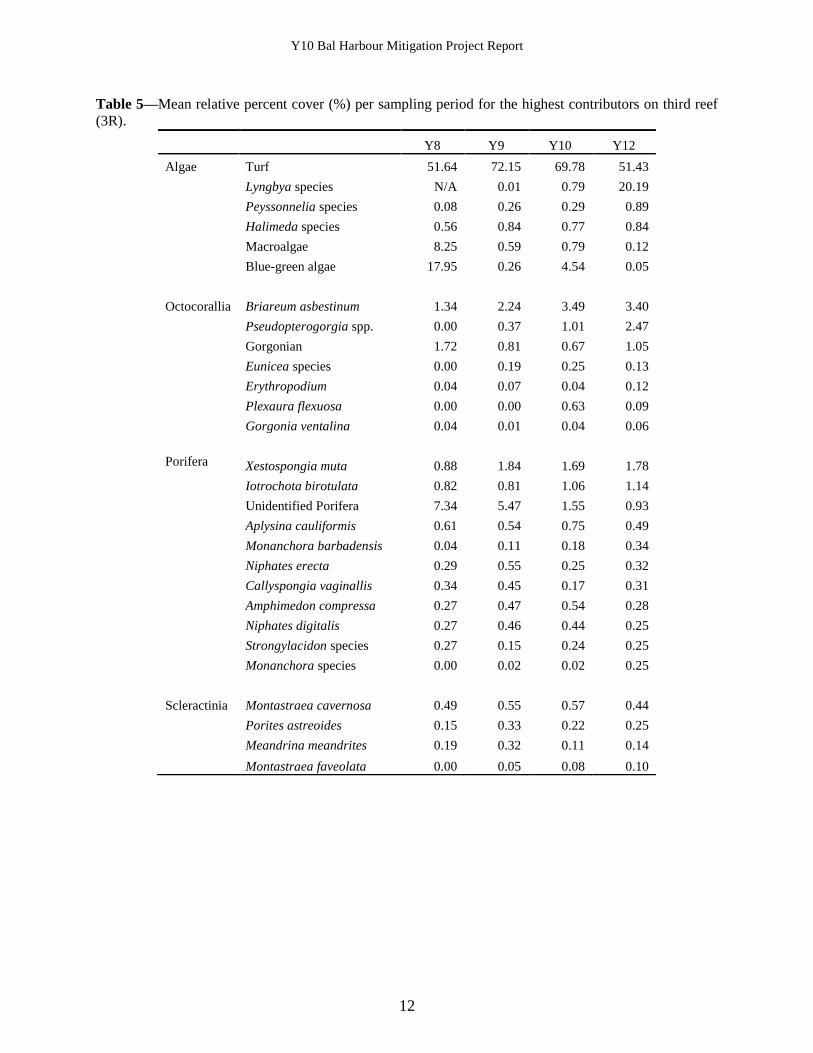
Table 5—Mean relative percent cover (%) per sampling period for the highest contributors on third reef

(3R).

Y8 Y9 Y10 Y12

Algae Turf 51.64 72.15 69.78 51.43

Lyngbya species N/A 0.01 0.79 20.19


Halimeda species 0.56 0.84 0.77 0.84

Macroalgae 8.25 0.59 0.79 0.12

Blue-green algae 17.95 0.26 4.54 0.05

Octocorallia Briareum asbestinum 1.34 2.24 3.49 3.40

Pseudopterogorgia spp. 0.00 0.37 1.01 2.47

Gorgonian 1.72 0.81 0.67 1.05

Eunicea species 0.00 0.19 0.25 0.13

Erythropodium 0.04 0.07 0.04 0.12

Plexaura flexuosa 0.00 0.00 0.63 0.09

Gorgonia ventalina 0.04 0.01 0.04 0.06

Porifera Xestospongia muta 0.88 1.84 1.69 1.78

Iotrochota birotulata 0.82 0.81 1.06 1.14

Unidentified Porifera 7.34 5.47 1.55 0.93


Monanchora barbadensis 0.04 0.11 0.18 0.34


Callyspongia vaginallis 0.34 0.45 0.17 0.31

Amphimedon compressa 0.27 0.47 0.54 0.28

Niphates digitalis 0.27 0.46 0.44 0.25

Strongylacidon species 0.27 0.15 0.24 0.25

Monanchora species 0.00 0.02 0.02 0.25

Scleractinia Montastraea cavernosa 0.49 0.55 0.57 0.44

Porites astreoides 0.15 0.33 0.22 0.25

Meandrina meandrites 0.19 0.32 0.11 0.14

Montastraea faveolata 0.00 0.05 0.08 0.10


13

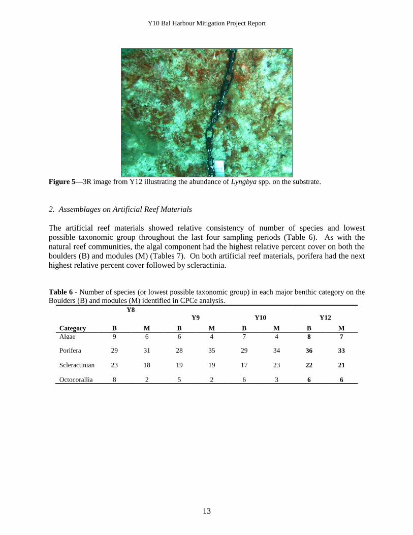
Figure 5—3R image from Y12 illustrating the abundance of Lyngbya spp. on the substrate.

2. Assemblages on Artificial Reef Materials

The artificial reef materials showed relative consistency of number of species and lowest

possible taxonomic group throughout the last four sampling periods (Table 6). As with the

natural reef communities, the algal component had the highest relative percent cover on both the

boulders (B) and modules (M) (Tables 7). On both artificial reef materials, porifera had the next

highest relative percent cover followed by scleractinia.

Table 6 - Number of species (or lowest possible taxonomic group) in each major benthic category on the

Boulders (B) and modules (M) identified in CPCe analysis.

Y8

Y9 Y10 Y12

Category B M B M B M B M

Algae 9 6 6 4 7 4 8 7

Porifera 29 31 28 35 29 34 36 33

Scleractinian 23 18 19 19 17 23 22 21

Octocorallia 8 2 5 2 6 3 6 6


14

Table 7—Relative percent cover (%) of major benthic taxa and substrate on the boulders (B). The ―other‖

benthic category includes Ascidiacia, Bivalvia, Gymnolaemata, Hydrozoa, and Polychaeta. The

―substrate‖ category refers to both barren hardbottom as well as sand or sediment covered areas.

Y8 Y9 Y10 Y12

Category Site Mean SD Mean SD Mean SD Mean SD

Algae B 83.00 4.69 80.03 2.05 85.25 0.40 81.85 1.76

M 79.01 1.51 72.18 1.36 70.01 1.77 67.66 2.59

Porifera B 14.00 4.26 11.14 2.24 10.17 0.95 11.94 0.76

M 18.83 1.31 24.12 0.47 26.36 1.73 26.12 1.94

Scleractinian B 1.21 0.52 2.01 0.23 1.65 0.09 1.94 0.09

M 0.80 0.22 1.46 0.38 1.74 0.46 2.21 0.40

Other B 0.31 0.15 0.39 0.13 0.60 0.25 1.27 0.62

M 0.32 0.11 0.69 0.21 0.52 0.15 1.99 0.76

Milliporidae B 0.17 0.07 0.32 0.20 0.16 0.11 0.18 0.10

M 0.61 0.04 0.88 0.31 0.69 0.31 1.14 0.36

Octocorallia B 0.33 0.14 0.54 0.19 1.62 1.10 1.77 0.76

M 0.02 0.02 0.04 0.04 0.05 0.05 0.19 0.16

Substrate B 0.93 0.33 0.57 0.36 0.54 0.32 1.05 0.61

M 0.32 0.26 0.55 0.54 0.47 0.17 0.70 0.37

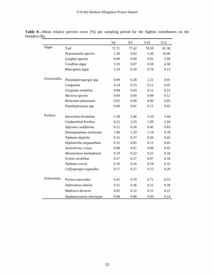
Table 8 shows the mean relative percent cover for the most common organisms on the boulders

(B). Similar to the natural reef sites (2R and 3R), the turf algae component had the highest

relative percent cover on the boulders. A notable change in the encrusting calcareous algae

components was observed in Y12. Both Peyssonnelia species and crustose coralline algae were

considerably higher on the boulders in Y12 than previous monitoring efforts. This is likely

attributed to the utilization of high resolution still images in Y12 opposed to lower quality

‗frame-grabbed‘ images from the video utilized in previous years. The video images produced

more points identified as a shadow or blurry especially on the vertical artificial reef surfaces.

Porifera was the next highest cover relative percent cover on the boulders, with the most

common species being I. birotulata, unidentified porifera, and A. cauliformis. Scleractinia had

the third highest cover on the boulders, with P. astreoides and Siderastrea siderea showing the

greatest cover of the 22 species identified through the coral point count methodology. Figure 6

shows representative transect images of the benthic growth on the boulders in Y12.


15

Table 8—Mean relative percent cover (%) per sampling period for the highest contributors on the

boulders (B).

Y8 Y9 Y10 Y12

Algae Turf 72.71 77.42 78.59 61.38


Lyngbya species 0.00 0.00 0.01 5.60


Blue-green algae 5.18 0.10 0.79 0.12

Octocorallia Pseudopterogorgia spp. 0.09 0.28 1.21 0.91

Gorgonian 0.14 0.23 0.11 0.45

Gorgonia ventalina 0.04 0.03 0.11 0.22

Muricea species 0.00 0.00 0.08 0.12


Pseudoplexaura spp. 0.00 0.01 0.11 0.02

Porifera Iotrochota birotulata 2.38 2.46 3.10 3.44





Diplastrella megastellata 0.31 0.05 0.11 0.45

Aiolochroia crassa 0.08 0.07 0.06 0.42


Ircinia strobilina 0.27 0.27 0.07 0.34



Scleractinia Porites astreoides 0.41 0.70 0.71 0.53

Siderastrea siderea 0.31 0.36 0.31 0.39

Madracis decactis 0.05 0.12 0.15 0.21

Stephanocoenia intersepta 0.08 0.08 0.09 0.14


16

Figure 6 – Transect images of benthic growth on the boulders in Y12.

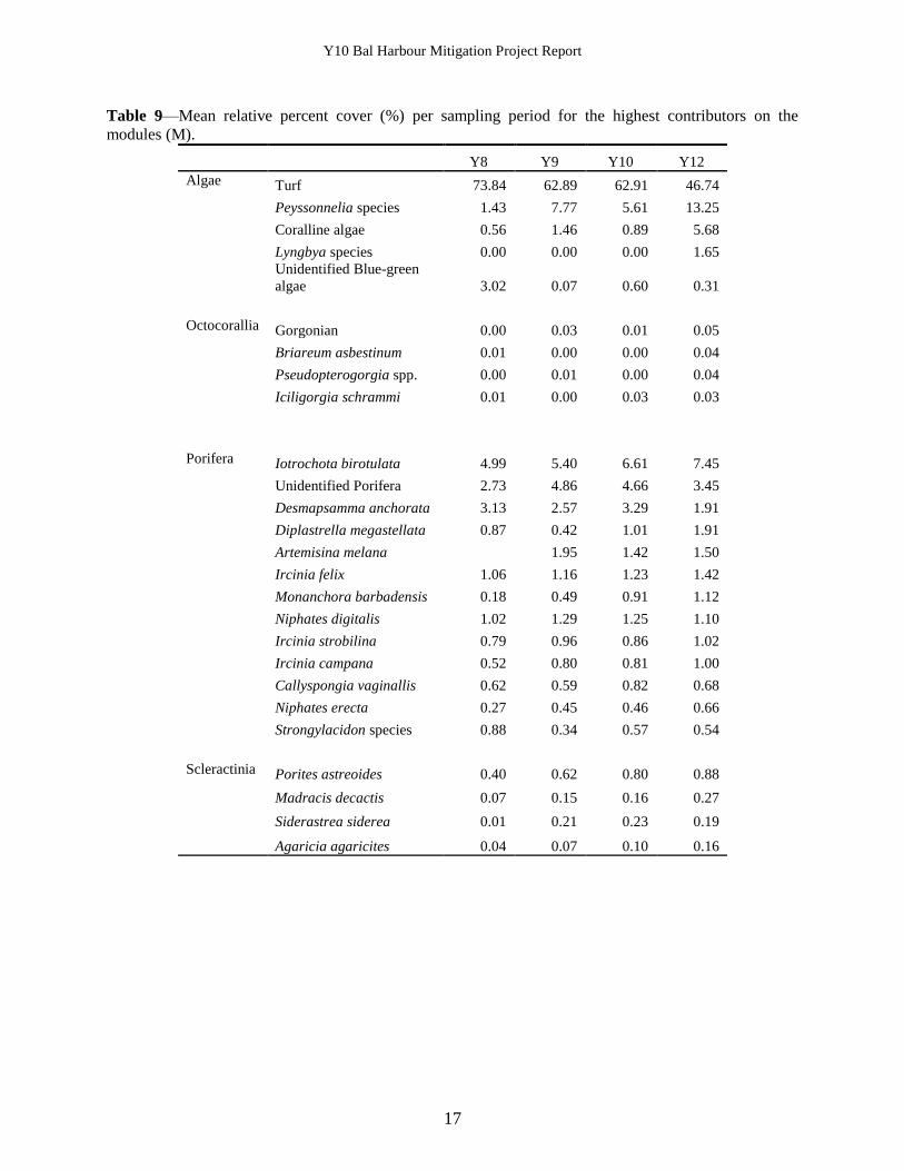
The mean relative percent cover for the most common organisms on the modules (M) is shown

in Table 9. The modules (M) were predominately covered by turf algae. A notable change in the

encrusting calcareous algae components was observed in Y12. Both Peyssonnelia species and

crustose coralline algae were considerably higher on the modules in Y12 than previous

monitoring efforts. This is likely attributed to the utilization of high resolution still images in

Y12 opposed to lower quality ‗frame-grabbed‘ images from the video utilized in previous years.

The video images produced more points identified as a shadow or blurry especially on the

vertical artificial reef surfaces. The modules had a higher percent cover of porifera than the

boulders as well as the natural reef sites with I. birotulata, unidentified porifera and

Desmapsamma anchorata showing the greatest cover. Other abundant porifera species in terms

of relative percent cover on the modules includes Diplastrella megastellata and Artemisina

melana. Porites astreoides and Madracis decactis were the scleractinian species with the highest

relative percent cover on the modules. Additionally, Tubastrea coccinea, a non-indigenous

species, was observed for the first time on the modules in Y9 and again in Y10 and Y12. Figure

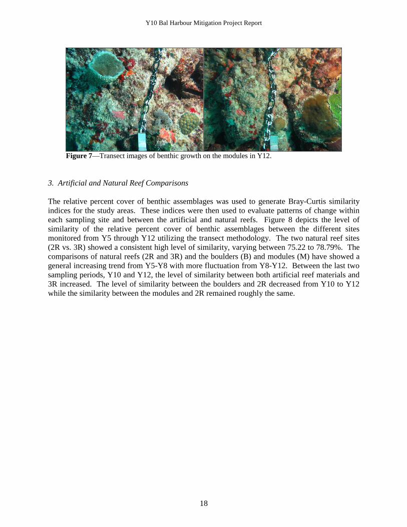
7 shows representative transect images of benthic growth on the modules in Y12.


17

Table 9—Mean relative percent cover (%) per sampling period for the highest contributors on the

modules (M).

Y8 Y9 Y10 Y12

Algae Turf 73.84 62.89 62.91 46.74



Lyngbya species 0.00 0.00 0.00 1.65

Unidentified Blue-green

algae 3.02 0.07 0.60 0.31

Octocorallia Gorgonian 0.00 0.03 0.01 0.05


Pseudopterogorgia spp. 0.00 0.01 0.00 0.04

Iciligorgia schrammi 0.01 0.00 0.03 0.03

Porifera Iotrochota birotulata 4.99 5.40 6.61 7.45



Diplastrella megastellata 0.87 0.42 1.01 1.91

Artemisina melana 1.95 1.42 1.50

Ircinia felix 1.06 1.16 1.23 1.42



Ircinia strobilina 0.79 0.96 0.86 1.02

Ircinia campana 0.52 0.80 0.81 1.00



Strongylacidon species 0.88 0.34 0.57 0.54

Scleractinia Porites astreoides 0.40 0.62 0.80 0.88

Madracis decactis 0.07 0.15 0.16 0.27

Siderastrea siderea 0.01 0.21 0.23 0.19

Agaricia agaricites 0.04 0.07 0.10 0.16


18

Figure 7—Transect images of benthic growth on the modules in Y12.

3. Artificial and Natural Reef Comparisons

The relative percent cover of benthic assemblages was used to generate Bray-Curtis similarity

indices for the study areas. These indices were then used to evaluate patterns of change within

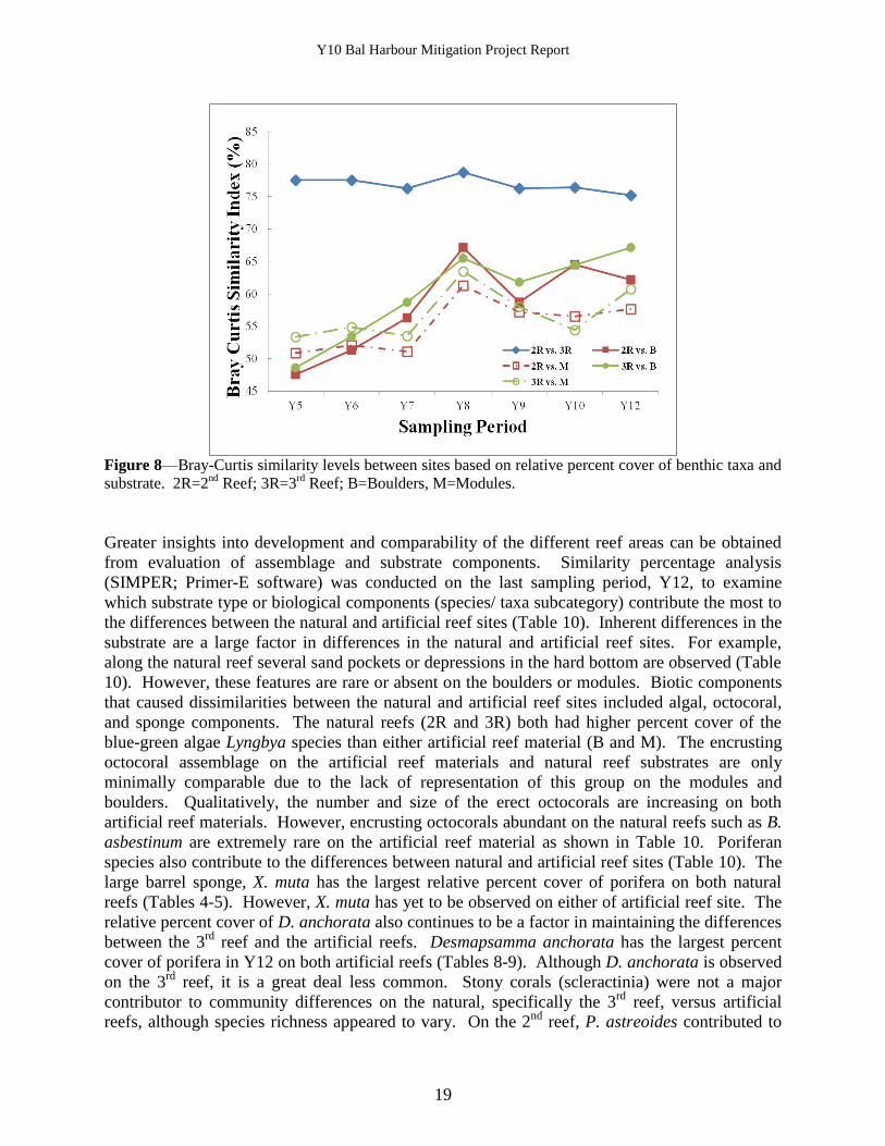
each sampling site and between the artificial and natural reefs. Figure 8 depicts the level of

similarity of the relative percent cover of benthic assemblages between the different sites

monitored from Y5 through Y12 utilizing the transect methodology. The two natural reef sites

(2R vs. 3R) showed a consistent high level of similarity, varying between 75.22 to 78.79%. The

comparisons of natural reefs (2R and 3R) and the boulders (B) and modules (M) have showed a

general increasing trend from Y5-Y8 with more fluctuation from Y8-Y12. Between the last two

sampling periods, Y10 and Y12, the level of similarity between both artificial reef materials and

3R increased. The level of similarity between the boulders and 2R decreased from Y10 to Y12

while the similarity between the modules and 2R remained roughly the same.


19

Figure 8—Bray-Curtis similarity levels between sites based on relative percent cover of benthic taxa and

substrate. 2R=2nd

Reef; 3R=3rd

Reef; B=Boulders, M=Modules.

Greater insights into development and comparability of the different reef areas can be obtained

from evaluation of assemblage and substrate components. Similarity percentage analysis

(SIMPER; Primer-E software) was conducted on the last sampling period, Y12, to examine

which substrate type or biological components (species/ taxa subcategory) contribute the most to

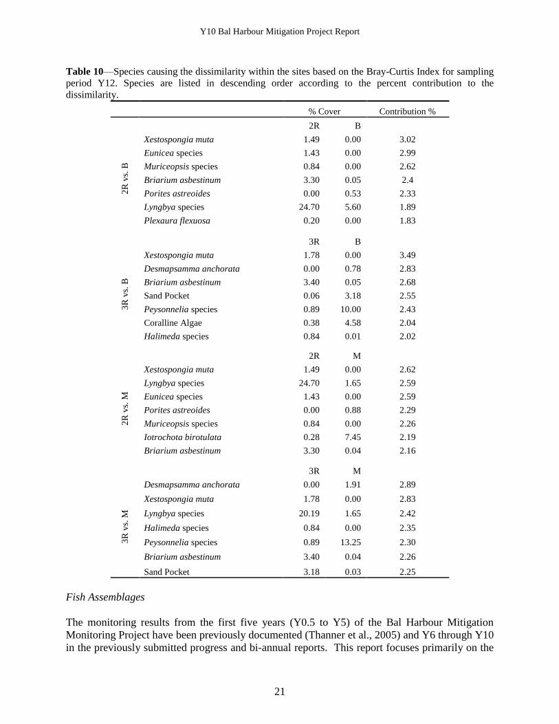
the differences between the natural and artificial reef sites (Table 10). Inherent differences in the

substrate are a large factor in differences in the natural and artificial reef sites. For example,

along the natural reef several sand pockets or depressions in the hard bottom are observed (Table

10). However, these features are rare or absent on the boulders or modules. Biotic components

that caused dissimilarities between the natural and artificial reef sites included algal, octocoral,

and sponge components. The natural reefs (2R and 3R) both had higher percent cover of the

blue-green algae Lyngbya species than either artificial reef material (B and M). The encrusting

octocoral assemblage on the artificial reef materials and natural reef substrates are only

minimally comparable due to the lack of representation of this group on the modules and

boulders. Qualitatively, the number and size of the erect octocorals are increasing on both

artificial reef materials. However, encrusting octocorals abundant on the natural reefs such as B.

asbestinum are extremely rare on the artificial reef material as shown in Table 10. Poriferan

species also contribute to the differences between natural and artificial reef sites (Table 10). The

large barrel sponge, X. muta has the largest relative percent cover of porifera on both natural

reefs (Tables 4-5). However, X. muta has yet to be observed on either of artificial reef site. The

relative percent cover of D. anchorata also continues to be a factor in maintaining the differences

between the 3rd

reef and the artificial reefs. Desmapsamma anchorata has the largest percent

cover of porifera in Y12 on both artificial reefs (Tables 8-9). Although D. anchorata is observed

on the 3rd

reef, it is a great deal less common. Stony corals (scleractinia) were not a major

contributor to community differences on the natural, specifically the 3rd

reef, versus artificial

reefs, although species richness appeared to vary. On the 2nd

reef, P. astreoides contributed to


20

the differences between both the boulders and the modules with greater cover on the artificial

reef materials. Stony coral species richness (based on CPCe analysis) in Y12 was highest on the

boulders with 22 species and on the modules with 21 species, while 2R and 3R had 8 and 10

species respectively (Tables 2, 6).


21

Table 10—Species causing the dissimilarity within the sites based on the Bray-Curtis Index for sampling

period Y12. Species are listed in descending order according to the percent contribution to the

dissimilarity.

% Cover Contribution %

2R B

2R

vs.

B

Xestospongia muta 1.49 0.00 3.02

Eunicea species 1.43 0.00 2.99

Muriceopsis species 0.84 0.00 2.62

Briarium asbestinum 3.30 0.05 2.4

Porites astreoides 0.00 0.53 2.33

Lyngbya species 24.70 5.60 1.89

Plexaura flexuosa 0.20 0.00 1.83

3R B

3R

vs.

B


Desmapsamma anchorata 0.00 0.78 2.83


Sand Pocket 0.06 3.18 2.55

Peysonnelia species 0.89 10.00 2.43

Coralline Algae 0.38 4.58 2.04

Halimeda species 0.84 0.01 2.02

2R M

2R

vs.

M



Eunicea species 1.43 0.00 2.59

Porites astreoides 0.00 0.88 2.29

Muriceopsis species 0.84 0.00 2.26

Iotrochota birotulata 0.28 7.45 2.19


3R M

3R

vs.

M

Desmapsamma anchorata 0.00 1.91 2.89



Halimeda species 0.84 0.00 2.35

Peysonnelia species 0.89 13.25 2.30


Sand Pocket 3.18 0.03 2.25

Fish Assemblages

The monitoring results from the first five years (Y0.5 to Y5) of the Bal Harbour Mitigation

Monitoring Project have been previously documented (Thanner et al., 2005) and Y6 through Y10

in the previously submitted progress and bi-annual reports. This report focuses primarily on the


22

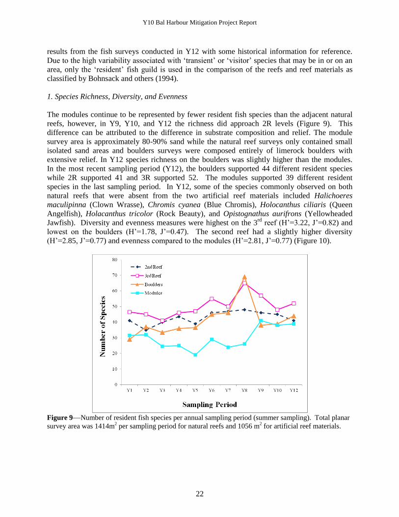
results from the fish surveys conducted in Y12 with some historical information for reference.

Due to the high variability associated with ‗transient‘ or ‗visitor‘ species that may be in or on an

area, only the ‗resident‘ fish guild is used in the comparison of the reefs and reef materials as

classified by Bohnsack and others (1994).

1. Species Richness, Diversity, and Evenness

The modules continue to be represented by fewer resident fish species than the adjacent natural

reefs, however, in Y9, Y10, and Y12 the richness did approach 2R levels (Figure 9). This

difference can be attributed to the difference in substrate composition and relief. The module

survey area is approximately 80-90% sand while the natural reef surveys only contained small

isolated sand areas and boulders surveys were composed entirely of limerock boulders with

extensive relief. In Y12 species richness on the boulders was slightly higher than the modules.

In the most recent sampling period (Y12), the boulders supported 44 different resident species

while 2R supported 41 and 3R supported 52. The modules supported 39 different resident

species in the last sampling period. In Y12, some of the species commonly observed on both

natural reefs that were absent from the two artificial reef materials included Halichoeres

maculipinna (Clown Wrasse), Chromis cyanea (Blue Chromis), Holocanthus ciliaris (Queen

Angelfish), Holacanthus tricolor (Rock Beauty), and Opistognathus aurifrons (Yellowheaded

Jawfish). Diversity and evenness measures were highest on the 3rd

reef (H‘=3.22, J‘=0.82) and

lowest on the boulders (H‘=1.78, J‘=0.47). The second reef had a slightly higher diversity

(H‘=2.85, J‘=0.77) and evenness compared to the modules (H‘=2.81, J‘=0.77) (Figure 10).

Figure 9—Number of resident fish species per annual sampling period (summer sampling). Total planar

survey area was 1414m2 per sampling period for natural reefs and 1056 m

2 for artificial reef materials.


23

Figure 10 - Mean Shannon Diversity Index and Pielou‘s Evenness measure for the resident fish

assemblages on 2nd

Reef, 3rd

Reef, Boulders and Modules in Y12. NOTE: Area of each survey = 176 m2.

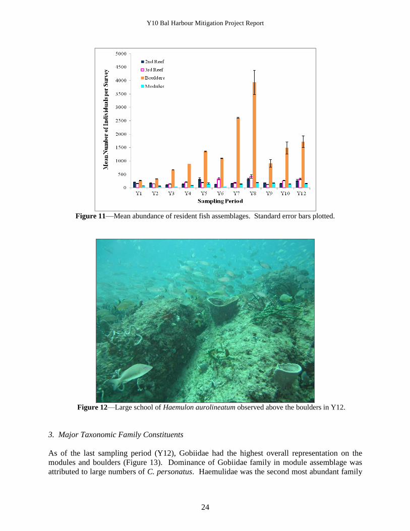
2. Abundance

Analysis of the ―resident‖ fish assemblage shows abundance differs greatly when comparing the

boulders and modules, as well as in the natural and artificial reef comparisons. The boulder site

has consistently shown the highest mean resident fish abundances (Figure 11). In Y12, the mean

abundance on the boulders was 1719.83 individuals per survey, mainly comprised of large

schools of Haemulon aurolineatum (524 ind. ±445.68) as seen in Figure 12 and large numbers of

juvenile and adult Coryphopterus personatus (925.17 ind. ±117.39) in the numerous void areas

in between boulders. In Y12 the modules had the lowest mean abundance of resident fish

followed by 2R and 3R respectively.


24

Figure 11—Mean abundance of resident fish assemblages. Standard error bars plotted.

Figure 12—Large school of Haemulon aurolineatum observed above the boulders in Y12.

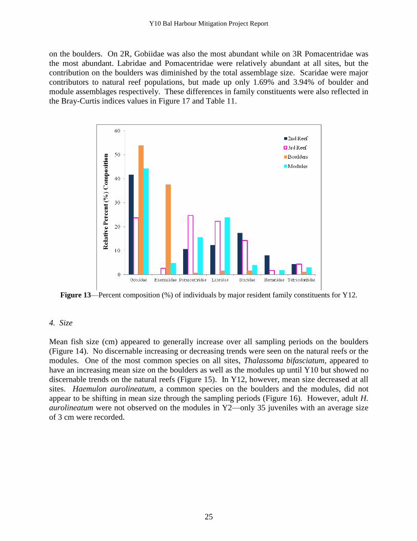
3. Major Taxonomic Family Constituents

As of the last sampling period (Y12), Gobiidae had the highest overall representation on the

modules and boulders (Figure 13). Dominance of Gobiidae family in module assemblage was

attributed to large numbers of C. personatus. Haemulidae was the second most abundant family


25

on the boulders. On 2R, Gobiidae was also the most abundant while on 3R Pomacentridae was

the most abundant. Labridae and Pomacentridae were relatively abundant at all sites, but the

contribution on the boulders was diminished by the total assemblage size. Scaridae were major

contributors to natural reef populations, but made up only 1.69% and 3.94% of boulder and

module assemblages respectively. These differences in family constituents were also reflected in

the Bray-Curtis indices values in Figure 17 and Table 11.

Figure 13—Percent composition (%) of individuals by major resident family constituents for Y12.

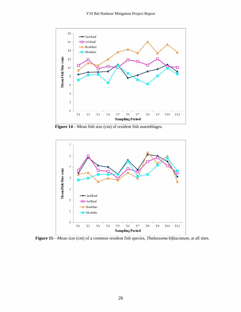
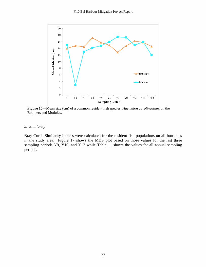
4. Size

Mean fish size (cm) appeared to generally increase over all sampling periods on the boulders

(Figure 14). No discernable increasing or decreasing trends were seen on the natural reefs or the

modules. One of the most common species on all sites, Thalassoma bifasciatum, appeared to

have an increasing mean size on the boulders as well as the modules up until Y10 but showed no

discernable trends on the natural reefs (Figure 15). In Y12, however, mean size decreased at all

sites. Haemulon aurolineatum, a common species on the boulders and the modules, did not

appear to be shifting in mean size through the sampling periods (Figure 16). However, adult H.

aurolineatum were not observed on the modules in Y2—only 35 juveniles with an average size

of 3 cm were recorded.


26

Figure 14—Mean fish size (cm) of resident fish assemblages.

Figure 15—Mean size (cm) of a common resident fish species, Thalassoma bifasciatum, at all sites.


27

Figure 16—Mean size (cm) of a common resident fish species, Haemulon aurolineatum, on the

Boulders and Modules.

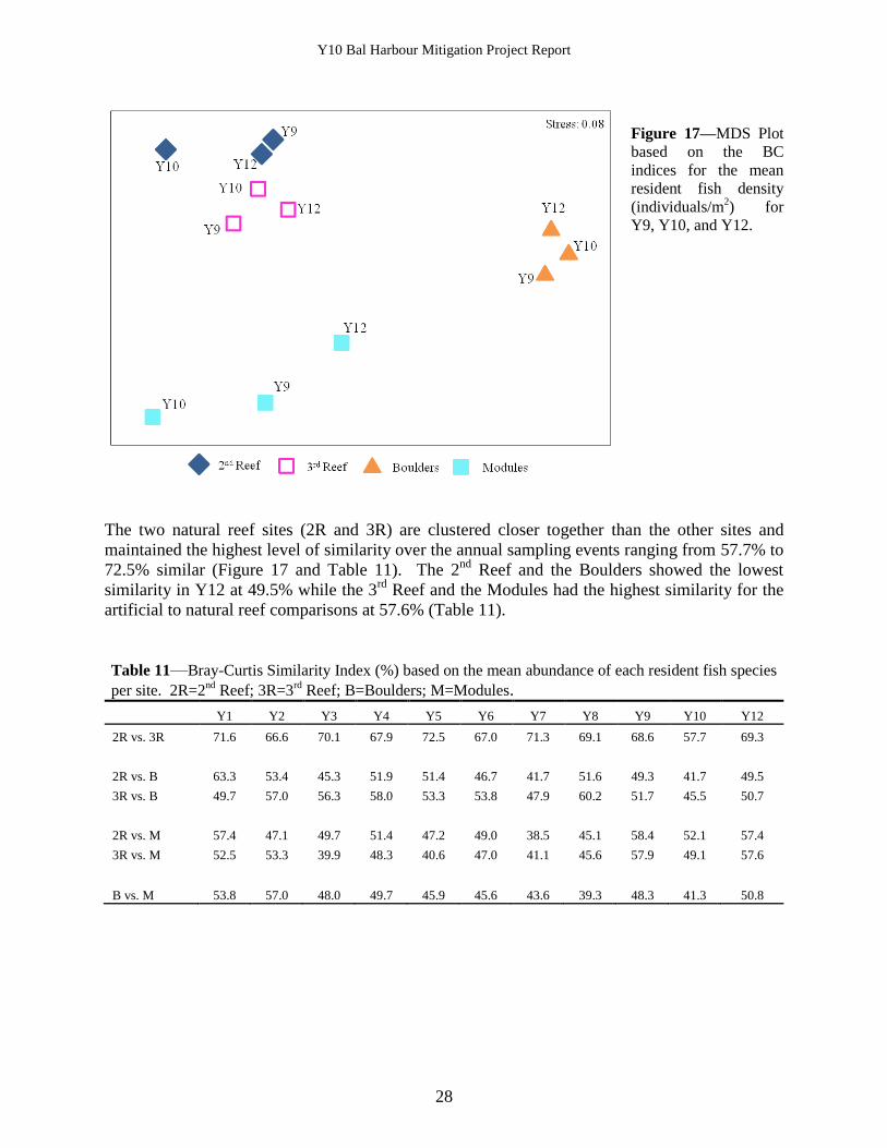
5. Similarity

Bray-Curtis Similarity Indices were calculated for the resident fish populations on all four sites

in the study area. Figure 17 shows the MDS plot based on those values for the last three

sampling periods Y9, Y10, and Y12 while Table 11 shows the values for all annual sampling

periods.


28

Figure 17—MDS Plot

based on the BC

indices for the mean

resident fish density

(individuals/m2) for

Y9, Y10, and Y12.

The two natural reef sites (2R and 3R) are clustered closer together than the other sites and

maintained the highest level of similarity over the annual sampling events ranging from 57.7% to

72.5% similar (Figure 17 and Table 11). The 2nd

Reef and the Boulders showed the lowest

similarity in Y12 at 49.5% while the 3rd

Reef and the Modules had the highest similarity for the

artificial to natural reef comparisons at 57.6% (Table 11).

Table 11—Bray-Curtis Similarity Index (%) based on the mean abundance of each resident fish species

per site. 2R=2nd

Reef; 3R=3rd

Reef; B=Boulders; M=Modules.

Y1 Y2 Y3 Y4 Y5 Y6 Y7 Y8 Y9 Y10 Y12

2R vs. 3R 71.6 66.6 70.1 67.9 72.5 67.0 71.3 69.1 68.6 57.7 69.3

2R vs. B 63.3 53.4 45.3 51.9 51.4 46.7 41.7 51.6 49.3 41.7 49.5

3R vs. B 49.7 57.0 56.3 58.0 53.3 53.8 47.9 60.2 51.7 45.5 50.7

2R vs. M 57.4 47.1 49.7 51.4 47.2 49.0 38.5 45.1 58.4 52.1 57.4

3R vs. M 52.5 53.3 39.9 48.3 40.6 47.0 41.1 45.6 57.9 49.1 57.6

B vs. M 53.8 57.0 48.0 49.7 45.9 45.6 43.6 39.3 48.3 41.3 50.8


29

Table 12—Species causing the dissimilarity within the sites based on the Bray-Curtis Index for sampling

period Y12. Species are listed in descending order according the percent contribution to the dissimilarity

(%).

Avg. Abundance Contribution %

2R 3R

2R

vs.

3R

Chromis multilineata 0.00 41.43 5.97

Serranus. tortugarum 24.80 0.00 1.61

Pareques acuminatus 0.00 18.00 4.85

Haemulon carbonarium 0.00 11.00 4.29

Malacoctenus triangulatus 0.00 6.00 3.68

2R B

2R

vs.

B

Haemulon aurolineatum 0.00 524.00 6.95

Haemulon flavolineatum 0.00 108.17 4.69

Haemulon chrysargyreum 0.00 72.33 4.24

Haemulon sciurus 0.00 54.17 3.94

Lutjanus griseus 0.00 31.60 3.45

3R B

3R

vs.

B



Haemulon sciurus 0.00 54.17 3.61

Coryphopterus personatus 69.00 925.17 3.50

Chromis multilineata 41..43 0.00 3.37

B M

B v

s. M



Coryphopterus personatus 925.17 56.50 4.45

Lutjanus synagris 26.40 0.00 3.64

Haemulon flavolineatum 108.17 1.33 3.45

2R M

2R

vs.

M

Sparisoma. chrysopterum 21.00 0.00 4.47

Cryptotomus roseus 9.50 0.00 3.67

Scarus taeniopterus 7.67 0.00 3.48

Scarus iserti 7.17 0.00 3.42

Anisotremis virginicus 0.00 7.00 3.40

3R M

3R

vs.

M

Pareques acuminatus 18.00 0.00 3.77

Cryptotomus roseus 14.67 0.00 3.58

Haemulon carbonarium 11.00 0..00 3.33

Scarus taeniopterus 10.67 0.00 3.31

Sparisoma chrysopterum 8.00 0.00 3.08

Clear distinctions still remain between the fish assemblages on the natural and artificial reef sites

as is shown by the low stress value of the MDS plot (Figure 17). This is also apparent through

the species richness (Figure 9), resident fish abundance (Figure 11), and major family

composition (Figure 13) previously described. The boulders and modules remain notably

divergent from one another as well as from the natural reef sites. The similarity levels between


30

the natural reefs and the artificial reef materials have fluctuated with no discernable trend. In

general, the modules are more similar to the natural reefs than the boulders. SIMPER analysis

of all surveys showed the species responsible for the dissimilarity between the natural reefs (2R

and 3R) and the modules was Sparisoma chrysopterum (2R) and Pareques acuminatus (3R) with

a greater abundance on the natural reefs. The large abundance of H. aurolineatum on the

boulders was responsible for the dissimilarity between both reef sites and the boulders.

Haemulon aurolineatum was also responsible for the difference between the boulders and the

modules with a greater abundance on the boulders (Table 12).


31

DISCUSSION

Artificial reefs are increasingly being utilized as mitigation for natural reef impacts. It is

important to understand the extent to which these ―reefs‖ can effectively provide habitat similar

to (i.e., mitigate for) natural reef areas. To gain an understanding of the extent to which these

reefs can fulfill this role, an evaluation must be conducted of the overall biotic community (i.e.,

benthic and fish assemblages) colonizing and utilizing the mitigation reef materials with those of

natural reef areas. Previous studies have documented that artificial substrates can provide habitat

for benthic invertebrates and fish (Bohnsack et al., 1994; G.M. Selby and Associates, 1994,

1995a, 1995b; Russel et al., 1974; Walker et al., 2002). Additionally, a study by Arena et al.

(2007) indicated that artificial (vessel) reefs may be a source of fish production rather than

attracting fish away from neighboring natural reefs. A study by Perkol-Finkel and Benayahu

(2005) in the Gulf of Eliat, Israel, suggested that it may take over ten years for an artificial reef

community to become diverse and mature. Results from a study in the United Arab Emirates

comparing a breakwater built in 1977 to nearby coral patches indicate higher coral cover on the

breakwater and suggest that it may take three or more decades for coral communities on artificial

reefs to develop enough for comparison with natural reefs (Burt et al., 2009). Another Perkol-

Finkel and Benayahu study (2007) indicated that physical structure of the artificial reef plays an

important role in recruitment comparisons to natural reef and therefore long term community

composition. This study says that for restoration purposes, the artificial reef must have similar

structural features to the natural reef. The Bal Harbour Mitigation Reef and adjacent natural

reefs have substantial differences in their structural features with increased relief and rugosity on

the mitigation reef which may restrict true similarity between the areas. The monitoring program

for the Bal Harbour Mitigation Reef is also only in the twelfth year and the mitigation may have

not yet reached the maximum similarity level with the natural reef is multiple decades are

required to achieve this.

Data from the first twelve years of monitoring program provide significant information on the

efficacy of the Bal Harbour Mitigation artificial materials to serve as natural reef mitigation.

Data throughout this study indicate that the local natural reefs support diverse and stable

communities. This is reflected in the similar species richness, and overall densities of the

benthic assemblages on the second and third reef stations (Table 2), as well as in the relative

consistency of the Bray-Curtis similarity values throughout the monitoring between these sites

(similarity values range between 75.22 to 78.79%; Figure 8). Similarly, the fish assemblages on

the natural reefs showed relatively consistent Bray-Curtis values (between 66.6 to 71.6%; Table

11).

The increase in similarity was rapid for the first few years of sampling and has been lower and

less discernable since (Thanner et al., 2006 and Y10 Progress Report and Summary, 2010). The

level of similarity between the benthic assemblages on both the modules and boulders and

natural reefs has remained somewhat consistent in Y8-Y12 (Figure 8). All sites maintain high

percent cover of algae—primarily turf algae (Tables 8 and 9). Both artificial reef materials

sustained higher percent poriferan cover than either natural reef site. On the natural reefs,

octocorals were the second most abundant taxonomic group while scleractinian corals were the

second most abundant group on the boulders and modules, primarily due to the presence of a

large number of juvenile corals. Scleractinian density on the artificial reefs continued to rise in


32

Y12 (Table 7). The percent cover of scleractinia on both the boulders and modules have been

comparable to that of (or above) 3R and above that found on 2R throughout the last four

sampling periods. The octocoral communities on the natural and artificial reefs though have

remained distinct. The mean relative percent cover by octocorals was 9.24% and 7.39%

respectively for 2R and 3R during the last sampling period Y12 (Table 3). Octocoral populations

appear to be increasing on the boulders during the last three sampling periods with a large

increase in Y10. There was a moderate increase in octocoral percent cover on the modules in

Y12. The percent cover of octocorals on the boulders was 0.54% in Y9, 1.62% in Y10 and

1.77% in Y12 only 0.04% in Y9, 0.06% in Y10 and 0.19 in Y12 on the modules (Table 7). The

reason for the disparity between octocoral communities on the natural reefs and the artificial

reefs can be partially attributed to the lack of encrusting octocoral development on the artificial

reef materials.

In general, resident fish populations demonstrated considerable variability. The fish assemblages

on the natural reefs were less variable than those on the artificial reef materials. Species richness

(Figure 9) and diversity and evenness measures (Figure 10) were generally higher on the natural

reefs. Fish abundance on the boulders continues to be greater than the modules and natural reefs

due to large schools of H. aurolineatum (Tomates) (Figure 11 and 12). The fish assemblages on

the boulders continue to be dominated by the Haemulidae family and by the Gobiidae family on

the modules (Figure 13). Mean fish size has varied on the boulders over the 12 years of

monitoring (Figure 18). Thalassoma bifasciatum (Bluehead) and H. aurolineatum (Tomtate)

size have varied throughout the monitoring period (Figures 15 and 16). Although the fish

assemblages do share some measure of similarity, the fish populations on the artificial reef

materials appeared to remain distinct in this study period. A portion of the variation seen the in

artificial reef fish assemblage over time may be associated with the documented change (i.e.,

development) of the benthic assemblages. Increased relief and complexity is considered a fish

‗attractant‘, and appears to play a role in the high densities of fish on the boulders; however, it is

interesting to note that while the modules provide a two to three fold increase in relief compared

to the adjacent reefs, the densities of fish are more comparable to the natural reef areas than the

boulders.

CONCLUSIONS

Although the level of similarity between the natural and artificial reefs has increased during the

twelve-year study, differences between natural and artificial reefs still remain. In addition to the

inherent differences in substrate, a significant contributor to the differences is the slow octocoral

development on the artificial reef materials, as well as differences in porifera composition. Fish

assemblages on the artificial and natural reefs, on the other hand, have not demonstrated

increases in similarity during this study. The similarity between sites does not appear to be

converging over time, rather maintaining distinct separation after twelve years, and possibly

showing divergence in similarity.

It does appear that the artificial reef structures are providing habitat for diverse benthic and fish

assemblages. Benthic assemblages have a moderately high level of similarity to the natural reefs

in species composition and relative species representation, which may indicate that the artificial


33

reef materials are developing communities that are comparable to the natural reef areas. Trends

identified in the benthic data indicate potential for continued convergence of the artificial and

natural population constituents with continued development of the octocoral assemblages. Fish

assemblages on the artificial reef do share many species in common with the natural reef areas.

Despite these similarities, however, the fish assemblages remain distinct between the natural and

artificial reef materials. Ultimately, physical differences between material types (i.e., shape,

relief, availability of cryptic habitat, etc) may limit the potential for these reefs to converge in

similarity. It is anticipated that future monitoring results will provide additional insights as to the

level to which the artificial reef materials are effective in serving as mitigation for the natural

reef impacts.


34

LITERATURE CITED

Arena, P.T., L.K.B. Jordan, R.E. Spieler. Fish assemblages on sunken vessels and natural reefs in

southeast Florida, U.S.A. 2007. Hydrobiologia 580: 157-171.

Blair, S.M. and B.S. Flynn. 1989. Biological monitoring of hard bottom reef communities off

Dade County Florida: Community description. Diving for Science 1989: 9-24.

Blair, S.M., B.S. Flynn, T. McIntosh, L.N. Hefty. 1990 Environmental impacts of the 1990 Bal

Harbour beach renourishment project: Mechanical and sedimentation impact on hard-

bottom areas adjacent to the borrow area. Metropolitan Dade County, Florida Department

of Environmental Resources. Technical Report 90-15. 46 pp.

Bohnsack, J.A. and S.P. Bannerot. 1986. A stationary visual census technique for quantitatively

assessing community structure of coral reef fishes. NOAA Technical Report NMFS 41.

15 pp.

____________, D.E. Harper, D.B. McClellan and M. Hulsbeck. 1994. Effects of reef size on

colonization and assemblage structure of fishes at artificial reefs off southeastern Florida,

USA. 1994. Bull. Mar. Sci. 55: 796-823.

Bray J.R. and J.T. Curtis. 1957. An ordination of the upland forest communities of Southern

Wisconsin. Ecol. Monog. 27:325-349.

Burt, J., A. Bartholomew, P. Usseglio, A. Bauman, and P.F. Sale. Are artificial reefs surrogates

of natural habitats for corals and fish in Dubai, United Arab Emirates? 2009. Coral Reefs

28: 663-675.

Clarke K.R. and R.M. Warwick R.M. 1994. Changes in Marine Communities: An Approach to

Statistical Analysis and Interpretation: 1st edition. Plymouth Marine Laboratory.

Plymouth, United Kingdom. 144p.

Consent Order. 1994. State of Florida Department of Environmental Protection vs. Dade County

Board of County Commissioners. OGC File No. 94-2842.

G.M. Selby and Associates, Inc. 1994. Sunny Isles Artificial Reef Monitoring Project Eighth

Quarterly Report—June 1994. Submitted to Miami-Dade County Department of

Environmental Resources Management.

. 1995a. Sunny Isles Artificial Reef Monitoring Project Twelfth Quarterly Report:

January 1995. Submitted to Miami-Dade County Department of Environmental

Resources Management.

. 1995b. Sunny Isles Artificial Reef Monitoring Project Sixteenth Quarterly Report:

September 1995. Submitted to Miami-Dade County Department of Environmental

Resources Management.

Field J.G., K.R. Clarke, and R.M. Warwick. 1982. A practical strategy for analyzing

multispecies distribution patterns. Mar. Ecol. Prog. Ser. 8: 37-52.

Florida Department of Environmental Protection. 1994. A Natural Resource Damage assessment

for the Bal Harbor Beach Renourishment Project. Technical Economic Report, DEP-

TER: 94-1. 19 pp.

Goldberg, W. 1973. The ecology of the coral-octocoral communities off the southeast Florida

coast: Geomorphology, species composition and zonation. Bull. Mar. Sci. 23:465-487.

Kohler, K.E. and S.M. Gill, 2006. Coral Point Count with Excel extensions (CPCe): A Visual

Basic program for the determination of coral and substrate coverage using random point

count methodology. Computers and Geosciences: 32 1259-1269.

Kruskal J.B. and M. Wish. 1978. Multidimensional Scaling. Sage Publications, Beverly


35

Hills, California. 93 p.

Lindeman, K.C. 1997. Development of Grunts and Snappers of Southeast Florida: Cross-shelf

distributions and effects of beach management alternatives. Ph.D. Dissertation 419 pp.

RSMAS, Univ. of Miami.

Moyer R.P., B. Riegl, K. Banks, and R. Dodge. 2003. Spatial Patterns and ecology of benthic

communities on a high-latitude south Florida (Broward County, USA) reef system. Coral

Reefs 22: 447-464.

Perkol-Finkel, S. and Y. Benayahu. 2005. Recruitment of benthic organisms onto a planned

artificial reef: shifts in community structure one decade post-deployment. Mar. Envi.

Res. 59: 79-99.

Perkol-Finkel, S. and Y. Benayahu. 2007. Differential recruitment of benthic communities on

neighboring artificial and natural reefs. Journal of Exp. Mar Bio. 340: 25-39.

Russell, B.C., F.H. Talbot, and S. Domm. 1974. Patterns of colonization of artificial reefs by

coral reef fishes. Proc. Int. Coral Reef Symp., 2nd

: 207-215.

Thanner, S.E., T.L. McIntosh, and S.M. Blair. 2006. Development of benthic and fish

assemblages on artificial reef materials compared to natural reef assemblages in Miami-

Dade County, Florida. Bull Mar Sci. 78: 57-70.

Walker B.K., B. Henderson, and R. Spieler. 2002. Fish assemblages associated with artificial

reefs of concrete aggregates or quarry stone offshore Miami Beach, Florida, USA. Aquat.

Living Resour. 15: 95-105.

Bal Harbour Mitigation Artificial Reef Monitoring … Harbour Mitigation Artificial Reef Monitoring...

Documents

Transcript of Bal Harbour Mitigation Artificial Reef Monitoring … Harbour Mitigation Artificial Reef Monitoring...