B4.3 Distribution Theory

Jan Kristensen

Michaelmas Term 2021

Contents

1 Background 2

1.1 Why Distributions? . . . . . . . . . . . . . . . . . . . . . . . . . . . . . . . . . . 3

1.1.1 One Dimensional Wave Equation . . . . . . . . . . . . . . . . . . . . . . 4

1.1.2 Laplace’s Equation . . . . . . . . . . . . . . . . . . . . . . . . . . . . . . 4

1.2 A brief review of some Calculus . . . . . . . . . . . . . . . . . . . . . . . . . . . 6

1.2.1 Classical derivatives . . . . . . . . . . . . . . . . . . . . . . . . . . . . . 7

1.2.2 Multi-index Notation . . . . . . . . . . . . . . . . . . . . . . . . . . . . . 11

2 Test functions 13

2.1 Support of a continuous function . . . . . . . . . . . . . . . . . . . . . . . . . . 13

2.2 Construction of test functions. . . . . . . . . . . . . . . . . . . . . . . . . . . . 14

2.2.1 The Standard Mollifier in Rn. . . . . . . . . . . . . . . . . . . . . . . . . 16

2.2.2 Cut-off Functions and Partitions of Unity . . . . . . . . . . . . . . . . . 19

2.3 Convergence in the sense of test functions . . . . . . . . . . . . . . . . . . . . . 20

3 Distributions 22

3.1 The definition. . . . . . . . . . . . . . . . . . . . . . . . . . . . . . . . . . . . . 22

3.2 Local Lebesgue Spaces. . . . . . . . . . . . . . . . . . . . . . . . . . . . . . . . 23

3.3 The boundedness property and the order of a distribution. . . . . . . . . . . . . 23

3.4 The fundamental lemma of the Calculus of Variations. . . . . . . . . . . . . . . 28

3.5 Convergence in the sense of distributions. . . . . . . . . . . . . . . . . . . . . . 29

4 Operations on distributions 31

1

4.1 Adjoint identities. . . . . . . . . . . . . . . . . . . . . . . . . . . . . . . . . . . 31

4.1.1 Differentiation in the sense of distributions . . . . . . . . . . . . . . . . 34

4.1.2 Multiplication by smooth function . . . . . . . . . . . . . . . . . . . . . 35

4.1.3 Convolution with test function . . . . . . . . . . . . . . . . . . . . . . . 37

4.2 Mollification and approximation of distributions. . . . . . . . . . . . . . . . . . 37

4.3 The Gauss-Green formula and some of its consequences. . . . . . . . . . . . . . 40

5 Some calculus for distributions 43

5.1 The basic theorems. . . . . . . . . . . . . . . . . . . . . . . . . . . . . . . . . . 43

5.1.1 The constancy theorem . . . . . . . . . . . . . . . . . . . . . . . . . . . 44

5.1.2 The fundamental theorem of calculus for distributions . . . . . . . . . . 45

5.1.3 Characterization of monotone functions . . . . . . . . . . . . . . . . . . 49

5.2 Sobolev functions. . . . . . . . . . . . . . . . . . . . . . . . . . . . . . . . . . . 51

5.3 Localization of distributions . . . . . . . . . . . . . . . . . . . . . . . . . . . . . 55

5.3.1 Support and singular support of a distribution . . . . . . . . . . . . . . 57

5.3.2 Compactly supported distributions . . . . . . . . . . . . . . . . . . . . . 59

6 Convolution of distributions and fundamental solutions 61

6.1 Convolution of distributions. . . . . . . . . . . . . . . . . . . . . . . . . . . . . 61

6.2 Fundamental solutions. . . . . . . . . . . . . . . . . . . . . . . . . . . . . . . . . 67

6.3 Elliptic regularity . . . . . . . . . . . . . . . . . . . . . . . . . . . . . . . . . . . 68

1 Background

The history of the theory of distributions is closely connected with the theory of PDEs. Proba-bly the first to use notions resembling that of distributions in mathematics were Fourier (1822),Kirchhoff (1882) and Heaviside (1898). More rigorous treatments followed, notably by Bochner(1932) who used, though implicitly, a notion of distribution in connection with his treatmentof the Fourier transformation, and in their studies of the Cauchy problem, Hadamard (1932)and M. Riesz (1949) considered certain special distributions. The first to rigorously definedistributions as linear functionals was Sobolev (1936). The closely related concept of weakderivatives, that arises naturally in the study of PDEs by variational methods, was also usedby Friedrichs (1939). However, it is only in the final form of Schwartz (1945–50), where alsothe Fourier transformation is an essential part, that distribution theory has become such aconvenient and efficient tool for the analysis of PDEs. This course and its sequel B4.4 Fourier

2

Analysis give an introduction to these topics.

1.1 Why Distributions?

The classical calculus for functions of several variables is inadequate if one seeks a simple andgeneral theory of PDEs. Borrowing an example from Hormander (1963) we consider the twoPDEs

∂2u

∂x∂y= 0 and

∂2u

∂y∂x= 0

for the real-valued function u = u(x, y) of two variables. The PDEs are equivalent for twicecontinuously differentiable functions u, but they are not equivalent for more general functions:the first PDE is satisfied by every function u = h(x) that depends on x alone, whereas thesecond PDE does not make sense for such functions when h(x) is not differentiable. Thisis somewhat unnatural and indicates the need for supplementing functions by new objects,distributions, so that differentiation is always possible and we get a better general notion ofsolution. In doing so it is important that we only add what is strictly necessary and that thenew objects obey, as close as possible, the usual calculus rules. In order to motivate the formaldefinition we consider the PDE

∂2u

∂x∂y= f in R2 (1)

where we assume that f = f(x, y) is a given continuous function. Assume first that u is atwice continuously differentiable solution of (1) and let φ : R2 → R be a twice continuouslydifferentiable function vanishing outside a bounded set. If we multiply (1) by φ, next integrateover R2 and perform two integrations by parts on the left-hand side (note the boundary termsdisappear because φ vanishes outside a bounded set) we arrive at∫∫

u∂2φ

∂y∂xdxdy =

∫∫fφ dxdy (2)

Note that we can recover (1) again from (2) when, as above, u is twice continuously differen-tiable, so that for such functions (1) and (2) are in fact equivalent. The advantage of (2) isthat it makes sense also when u is not twice continuously differentiable, for example it wouldsuffice to assume that u is continuous (or merely locally integrable). It is also not difficult tosee, that for a given u as above, the identity (2) cannot hold for more than one continuousfunction f (compare the Fundamental Lemma of the Calculus of Variations in Subsection 3.4below). This makes it natural to define ∂2u/∂x∂y = f in the weak sense if the identity (2)holds for all functions φ that are twice continuously differentiable and vanish off a boundedset. Since ∂2φ/∂x∂y = ∂2φ/∂y∂x for twice continuously differentiable functions φ it is clearthat the PDEs ∂2u/∂x∂y = f and ∂2u/∂y∂x = f then become equivalent in the weak sense.The theory of distributions goes a step further and considers the linear functional

φ 7→∫∫

u∂2φ

∂x∂ydxdy

3

as a representation for ∂2u/∂x∂y even when there is no continuous function f for which (2)holds. In order to be able to study PDEs of any order we are thus led to consider linearfunctionals on the set of functions vanishing outside bounded sets and having continuousderivatives of any order.

Perhaps it is still not clear from the above why we should bother to introduce objects,distributions, that can always be differentiated. Our next example is taken from Strichartz’sbook A Guide to Distribution Theory and Fourier Transforms.

1.1.1 One Dimensional Wave Equation

The equation∂2u

∂t2(x, t) = k2

∂2u

∂x2(x, t) (3)

can be used to model a vibrating string. A function given by

u(x, t) = f(x− kt),

where f is a function of one variable, represents a travelling wave with shape f(x) moving tothe right with velocity k. When f is twice differentiable, one can check that u is a solutionto (3). However, there is no physical reason for the shape of the travelling wave to be twicedifferentiable. For instance, the triangular profile

@

@@

@@@

-

moving with speed k to the right is perfectly fine! We do not want to throw away physicallymeaningful solutions because of technicalities. Looking at the example above, one could thinkthat if we accepted as solutions to differential equations any function that satisfies the differ-ential equation except for some points (finitely many, say), where it fails to be differentiable,then all would be fine. But this would be a much too simplistic general principle, as the nextexample shows.

1.1.2 Laplace’s Equation

In the plane R2 we have Laplace’s equation

∆u ..=∂2u

∂x2+∂2u

∂y2= 0. (4)

A solution to the above equation has the physical interpretation of an electric potential in aregion with no external charges. From physical experience it is known that such potentials

4

should be smooth. However, as you may have seen last year,

u = G0 :=1

4πlog

(x2 + y2

),

is a solution in R2 \ (0, 0). Clearly it cannot be extended to the origin in a smooth manner,and so it should not be considered as a solution to (4) on the full plane.

Distribution theory allows us, among many other things, to distinguish between the case ofthe one dimensional wave equation (3) and Laplace’s equation (4). Indeed, the standing wavesatisfies the one dimensional wave equation in the sense of distributions for any continuousprofile f , whereas

∆G0 = δ0

as distributions, where δ0 is Dirac’s delta function, a distribution.

But there are in fact many other reasons to study distributions, and most of them areonly really appreciated after the fact. Many physical quantities are naturally not definedpointwise. For instance, being able to measure temperature at a given point in space and timeis an idealization – see the discussion in Strichartz’s book A Guide to Distribution Theoryand Fourier Transforms, §1. Similarly, in the theory of Lebesgue integration as discussedin the Part A Integration course you encountered Lp functions. Strictly speaking they arenot functions, but equivalence classes of functions under the equivalence relation equal almosteverywhere. Nonetheless, for f ∈ Lp(Rn) and each measurable subset A of Rn the bracket

〈f,1A〉 ..=

∫Af(x) dx where now x = (x1 , . . . , xn) (5)

is well-defined and does not depend on the particular representative used to calculate theintegral. Note that if we know that f has a continuous representative, then we can uniquelydetermine the value of this continuous representative at all points x ∈ Rn from the values ofthe integrals (5) for all measurable subsets A of Rn. In fact, we do not need the values in (5)for all measurable sets. For instance, it would suffice to know them for all open balls Br(x0)since we have (denoting the continuous representative again by f) that

1

L n(Br(x0))

∫Br(x0)

f(x) dx→ f(x0) as r 0 (6)

for all x0 ∈ Rn. On the other hand, for a general Lp function f , knowing the values of theintegrals (5) for all measurable subsets A of Rn determines f(x) uniquely almost everywhere,or more precisely, uniquely as an Lp function. (In fact, the assertion (6) remains true for almostall x0 ∈ Rn when f is a general Lp function: the limit of the left-hand side exists in R foralmost all x0 ∈ Rn and defines a representative for the Lp function. This is a consequence ofLebesgue’s Differentiation Theorem.) Note that here the indicator function of the set A,

1A(x) =

1 if x ∈ A,0 if x /∈ A

5

acts as a test function, or measurement of f , and instead of thinking about f as the basicobject we could equally well consider the functional 1A 7→ 〈f,1A〉 to be the basic object.(Terminology : Functional means the same as function, but is often used instead if we havea real or complex-valued function defined on other functions.) It turns out that taking verynice test functions here is a good idea that allows us to extend aspects of differential calculusto Lp functions and beyond. This leads to the theory of distributions. Before getting therewe must spend some time developing our notion of a test function. It is worth mentioningthat there is not just one class of test functions. In this course and its sequel Fourier Analysiswe shall systematically investigate two such classes: the compactly supported ones and theSchwartz ones. But for particular problems it is often the case that it is more natural to useother classes of test functions. To each class of test functions there corresponds a class ofdistributions. The principle to keep in mind here is that the nicer the test functions are, therougher the corresponding distributions are allowed to be and vice versa. The general principlebehind all of this is that of duality. You encountered it in a purely algebraic form already inLinear Algebra and if you follow the Functional Analysis courses this year you will see it againthere.

1.2 A brief review of some Calculus

We start by fixing some notation. On Rd we shall usually employ the standard euclidean normthat is defined by the dot product:

|x| :=√x · x =

√x21 + . . . + x2d.

Here the dimension d is understood from context and not emphasized in our notation. Theopen ball with centre x0 and radius r is

Br(x0) :=x ∈ Rd : |x− x0| < r

.

The corresponding closed ball is denoted with a bar on top, Br(x0). Similarly, the closure ofany subset A of Rd is A. Occasionally we shall also write Br(A) which is taken to mean ther-metric neighbourhood of the set A:

Br(A) :=⋃a∈A

Br(a).

For two arbitrary subsets A and B of Rd we define the distance between them to be

dist(A,B) := inf|a− b| : a ∈ A, b ∈ B

.

We use the convention that the infimum of the empty set is +∞ so that the distance betweenA and B is always defined, but possibly +∞. We record in particular that if K is a compactsubset of an open set V in Rd, then the distance

dist(K,Rd \ V ) := inf|x− y| : x ∈ K, y ∈ Rd \ V

> 0. (7)

6

For two open subsets U and V of Rd we write U ⋐ V if U is compact and U ⊂ V . Clearly wethen also have that dist(U,Rd \ V ) > 0 when U ⋐ V .

When A = x and B is a general subset we write dist(x,B) := dist(x, B) and it is notdifficult to check that the function Rd 3 x 7→ dist(x,B) is 1-Lipschitz: |dist(x,B)−dist(y,B)| ⩽|x− y| holds for all x, y ∈ Rd.

1.2.1 Classical derivatives

Next we recall that a function f : S → R defined on a subset S of R is said to be differentiableat a point x0 if x0 is an interior point of S and the difference quotient

f(x)− f(x0)

x− x0, x ∈ S \ x0,

has a limit in R as x→ x0. Of course this limit is the differential quotient of f at x0, denotedas usual by f ′(x0). The above generalizes in a straight forward manner to the case wherethe function f is complex valued, so f : S → C, and to the case where it is Rk-valued, sof : S → Rk. In all cases we retain the notation f ′(x0) for the differential quotient when itexists.

It is well-known that we can relate the value of a differentiable function f : (a, b) → R toits derivative via the Mean Value Theorem. If f is continuously differentiable, then we evenhave that

f(x) = f(x0) +

∫ x

x0

f ′(t) dt

for all x, x0 ∈ (a, b) by the Fundamental Theorem of Calculus. While the latter remainstrue also for vector-valued functions, the Mean Value Theorem breaks down in that case (forinstance try f(x) = eix, x ∈ R, between 0 and 2π). The following weaker result can thensometimes be used instead.

Proposition 1.1. (The Mean Value Inequality)

Let I ⊆ R be an open interval and assume that f : I → Rd is differentiable. Then

|f(y)− f(x)| ⩽ |y − x| supt∈(0,1)

|f ′(x+ t(y − x)

)|

holds for all x, y ∈ I.

Proof. There is nothing to prove if the supremum on the right-hand side is +∞ (we use theconvention that the supremum of a set that is not bounded above is +∞). Assume thereforethat it is finite and fix

M > supt∈(0,1)

|f ′(x+ t(y − x)

)|. (8)

7

Now to prove the desired inequality it suffices to do it for the case where x, y ∈ I satisfy x > y.We fix such a pair and define the set

E =t ∈ [0, 1] : |f(x+ t(y − x))− f(x)| ⩽Mt|x− y|

.

Clearly 0 ∈ E and because f is continuous the set E must be closed relative to [0, 1]. It followsthat it has a largest element, say s = maxE. Because I is open and x+ s(y − x) ∈ I we haveby differentiability that for t > s with t− s sufficiently small,

|f(x+ t(y − x))− f(x+ s(y − x))| ⩽M(t− s)|y − x|.

Consequently we find

|f(x+ t(y − x))− f(x)| ⩽ |f(x+ t(y − x))− f(x+ s(y − x))|+ |f(x+ s(y − x))− f(x)|⩽ M(t− s)|y − x|+Ms|y − x|= Mt|y − x|,

hence s = 1. Because M was arbitrary in (8) the proof is complete.

Corollary 1.2. Let I ⊆ R be an open interval and C a closed subset of I. Suppose thatf : I → Rd is continuous, differentiable on I \ C and f(x) = 0 for x ∈ C. If x ∈ C and

f ′(y) → 0 as I \ C 3 y → x, (9)

then f ′(x) exists and equals 0.

Proof. If y ∈ C, then f(y)− f(x) = 0 and all is fine. We then consider the case y ∈ I \C andcan assume that y > x as the situation when y < x is entirely similar. Fix such y and let z bethe point in C ∩ [x, y] that is closest to y (why does it exist?). Then as f is differentiable onthe interval (z, y) we get from the Mean Value Inequality

|f(y)− f(x)| = |f(y)− f(z)| ⩽ |y − z| supt∈(0,1)

|f ′(z + t(y − z))|

and so|f(y)− f(x)|

|y − x|⩽ sup

t∈(0,1)|f ′(z + t(y − z))|.

Observe that |z + t(y − z) − x| ⩽ |y − x| for all t ∈ (0, 1) so using the assumption (9), givenε > 0 we find δ > 0 with the property that

|f ′(a)| < ε for all a ∈ (x, x+ δ) ∩ I \ C

and the conclusion follows.

8

Example 1.3. Let P (x) ∈ C[x] be a polynomial and define the function

f(x) =

P(1x

)e−

1x if x > 0

0 if x ⩽ 0.

Then f is easily seen to be continuous everywhere and differentiable for x 6= 0 with

f ′(x) =

e−

1x(P(1x

)− P ′( 1

x

))/x2 if x > 0

0 if x < 0.

This is of course just the same form as that of f and so we conclude from Corollary 1.2 (orsimply by use of the definition) that f ′(0) exists and equals 0. An easy induction argumentnow shows that f is infinitely often differentiable.

For functions of several variables we have partial derivatives and directional derivatives.Let ejnj=1 be the standard basis for Rn and assume that f : S → R is a real-valued function(or it could be complex or vector valued), where now S is a subset of Rn. We then say that fhas a partial derivative with respect to xj at x0 if x0 is an interior point of S and the differencequotient

f(x0 + hej)− f(x0)

h, h ∈ R \ 0 and x0 + hej ∈ S

has a limit in R as h → 0. This limit is the partial derivative at x0 that we shall denote byvarious different symbols, including

∂jf(x0) = ∂xjf(x0) = Djf(x0) =∂f

∂xj(x0) = fxj (x0) = . . . . . .

A slight variation of the above yields directional derivatives: replace ej by a general vectorv ∈ Rn \ 0 to define ∂vf(x0). When f has all first order partial derivatives at the point x0we can collect them in a vector:

∇f(x0) :=(∂1f(x0) . . . , ∂nf(x0)

)=

n∑j=1

∂jf(x0)ej .

This is the gradient of f at x0. When f is Rd-valued, say f = (f1, . . . , fd)† (we think of f as a

column vector, hence the transpose) it is customary to collect the first order partial derivatives(when they exist) in a matrix called the Jacobi matrix for f at x0:

∇f(x0) = Df(x0) :=[∂1f(x0) . . . ∂nf(x0)

]=

∂1f1(x0) . . . ∂nf1(x0). . . . . . . . . . . . . . . . . . . . .. . . . . . . . . . . . . . . . . . . . .∂1fd(x0) . . . ∂nfd(x0)

∈ Rd×n.

It is perfectly possible for a function, say f : R2 → R, to have directional derivatives in alldirections at (0, 0) and at the same time be discontinuous there. It can also happen that∂vf(0, 0) 6= ∇f(0, 0) ·v for some vectors v. However, these pathological situations are excludedif the function is continuously differentiable, meaning that ∂1f, . . . , ∂nf all exist and arecontinuous. More precisely we have the following:

9

Lemma 1.4. Let S be a subset of Rn and let x0 be an interior point of S. Assume thefunction f : S → Rd has partial derivatives ∂1f(x), . . . , ∂nf(x) for all x in a neighbourhoodof x0 and that they are all continuous at x0, then f is continuous at x0 and we have that∂vf(x0) = ∇f(x0)v for all v ∈ Rn \ 0.

The proof is an exercise.

The higher order partial derivatives are defined inductively. For instance, if we say that themixed partial derivative ∂2f/∂xj∂xk exists at the point x0 for the function f : S → Rd, then itmeans that x0 is an interior point of S, that ∂f/∂xk exists in a neighbourhood of x0 and has apartial derivative with respect to xj at x0. Note that in this generality it is important that wepay attention to the order in which we partially differentiate. We are actually not interestedin such situations and shall mostly be working with classes of functions where this is no issue.

Definition 1.5. Let Ω be a non-empty open subset of Rn and let k ∈ N. Then a functionf : Ω → R (or complex or vector-valued) is said to be k times continuous differentiable if allpartial derivatives of f up to and including order k exist and are continuous throughout Ω.

Example 1.6. The function f is continuously differentiable if f is continuous and all the partialderivatives ∂f/∂x1, . . . , ∂f/∂xn exist and are continuous on Ω. Note in particular that werequire, for example, ∂f/∂x1 to be jointly continuous in x = (x1, x2, . . . , xn) ∈ Ω.

Likewise, f is twice continuously differentiable if f is continuous and all the partial deriva-tives ∂f/∂xi, i = 1, . . . , n, ∂2f/∂xj∂xk, j, k = 1, . . . , n exist and are continuous on Ω.

In this connection the following notation is standard.

C(Ω) ..= u : Ω → R : u is continuous.

Similarly, for k ∈ N we define

Ck(Ω) ..= u : Ω → R : u is k times continuously differentiable.

We say that such functions are Ck functions. When k = 0 we write also C0(Ω) = C(Ω).

Note that Ck(Ω) is descending in k, Ck+1(Ω) ⊊ Ck(Ω). We define

C∞(Ω) ..=∞⋂k=0

Ck(Ω),

the class of infinitely differentiable functions on Ω. We remark that under the natural pointwisedefinitions of addition, multiplication by scalars, and multiplication, these classes all formcommutative rings with unity and vector spaces.

The same notation will be used for complex and vector-valued functions (where of course inthe vector-valued case the spaces cease to be rings).

Ck functions are well-behaved:

10

Lemma 1.7. If f : Ω → R is C2, then

∂2f

∂xj∂xk=

∂2f

∂xk∂xj(1 ⩽ j, k ⩽ n)

on Ω. Hence the order in which we take (two) partial derivatives is unimportant for C2 func-tions.

Proof. Let ejnj=1 be the standard basis for Rn and denote by

4hf(x) ..= f(x+ h)− f(x)

the increment in f at x corresponding to the increment h in x, where we must assume x, x+h ∈Ω. Observe that 4sej4rekf(x) = 4rek4sejf(x) holds for x ∈ Ω and s, r ∈ R with |s|, |r|sufficiently small. Because f is C2 we may apply the Fundamental Theorem of Calculus twicewhereby we find

1

sr4sej4rekf(x) =

∫ 1

0

∫ 1

0

∂2f

∂xj∂xk(x+ σsej + ρrek) dσ dρ,

and hence ∣∣∣∣ 1sr4sej4rekf(x)−∂2f

∂xj∂xk(x)

∣∣∣∣ → 0

as (r, s) → (0, 0).

We can extend this result to Ck functions and arbitrary k-th order partial derivatives for k ⩾ 2by induction, and so for such functions we do not have to worry about the order in whichwe partially differentiate. When there are many independent variables we shall often rely onmulti-index notation.

1.2.2 Multi-index Notation

A multi-index α is an n-tuple of non-negative integers, α = (α1, . . . , αn) ∈ Nn0 . The length (ororder) of α is

|α| ..= α1 + · · ·+ αn.

If α, β ∈ Nn0 and j ∈ N0, then also α + jβ ∈ Nn0 . For a multi-index α ∈ Nn0 we define itsfactorial as

α! := α1!α2! . . . αn!

and for an n-tuple x = (x1, . . . , xn) of real or complex numbers we write

xα := xα11 · . . . · xαnn .

11

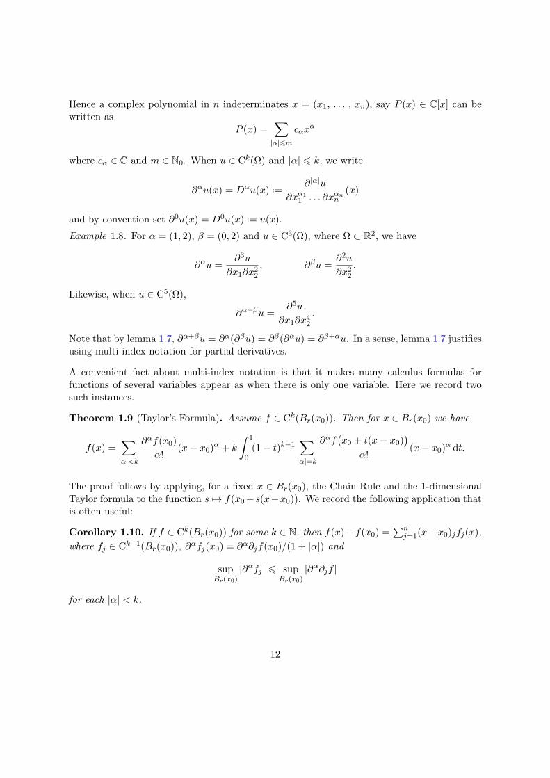
Hence a complex polynomial in n indeterminates x = (x1, . . . , xn), say P (x) ∈ C[x] can bewritten as

P (x) =∑

|α|⩽mcαx

α

where cα ∈ C and m ∈ N0. When u ∈ Ck(Ω) and |α| ⩽ k, we write

∂αu(x) = Dαu(x) ..=∂|α|u

∂xα11 . . . ∂xαnn

(x)

and by convention set ∂0u(x) = D0u(x) ..= u(x).

Example 1.8. For α = (1, 2), β = (0, 2) and u ∈ C3(Ω), where Ω ⊂ R2, we have

∂αu =∂3u

∂x1∂x22, ∂βu =

∂2u

∂x22.

Likewise, when u ∈ C5(Ω),

∂α+βu =∂5u

∂x1∂x42.

Note that by lemma 1.7, ∂α+βu = ∂α(∂βu) = ∂β(∂αu) = ∂β+αu. In a sense, lemma 1.7 justifiesusing multi-index notation for partial derivatives.

A convenient fact about multi-index notation is that it makes many calculus formulas forfunctions of several variables appear as when there is only one variable. Here we record twosuch instances.

Theorem 1.9 (Taylor’s Formula). Assume f ∈ Ck(Br(x0)). Then for x ∈ Br(x0) we have

f(x) =∑|α|<k

∂αf(x0)

α!(x− x0)

α + k

∫ 1

0(1− t)k−1

∑|α|=k

∂αf(x0 + t(x− x0)

)α!

(x− x0)α dt.

The proof follows by applying, for a fixed x ∈ Br(x0), the Chain Rule and the 1-dimensionalTaylor formula to the function s 7→ f(x0+s(x−x0)). We record the following application thatis often useful:

Corollary 1.10. If f ∈ Ck(Br(x0)) for some k ∈ N, then f(x)−f(x0) =∑n

j=1(x−x0)jfj(x),where fj ∈ Ck−1(Br(x0)), ∂

αfj(x0) = ∂α∂jf(x0)/(1 + |α|) and

supBr(x0)

|∂αfj | ⩽ supBr(x0)

|∂α∂jf |

for each |α| < k.

12

Proof. We use the formula for k = 1, which actually amounts to the Fundamental Theorem ofCalculus, whereby the Corollary is seen to hold with

fj(x) =

∫ 1

0(∂jf)

(x0 + t(x− x0)

)dt.

The assertions about fj all follow by inspection.

Theorem 1.11 (Generalized Leibniz Rule). Let f, g ∈ Ck(Ω). Then fg ∈ Ck(Ω) and forα ∈ Nn0 , |α| ⩽ k, we have

∂α(fg) =∑β⩽α

(α

β

)∂βf∂α−βg,

where β ⩽ α means βi ⩽ αi for all i = 1, . . . n,(α

β

)..=

α!

β!(α− β)!.

Proof. This can be proven by induction on the order |α| of differentiation, using the Leibnizrule

∂j(fg) = g∂jf + f∂jg

in the induction step.

2 Test functions

2.1 Support of a continuous function

For u ∈ C(Ω) we define the support of u as

supp(u) ..= Ω ∩ x ∈ Ω : u(x) 6= 0,

that is, the closure of the set u 6= 0 relative to Ω. As such, supp(u) is closed in Ω, but neednot be closed in Rn.Example 2.1. Define u1 : R → R by

u1(x) =

1− |x|, |x| < 1,0, |x| ⩾ 1.

Then supp(u1) = [−1, 1]. If instead we consider the restriction of u1 to Ω = (−1, 1), that is,u2(x) = 1− |x|, x ∈ (−1, 1), then supp(u2) = (−1, 1).

One sees that the support of a function u depends on the domain Ω, and we could emphasizethis and instead write suppΩ(u). However, for our purposes it will suffice to write supp(u),where Ω will be understood from context.

In the following we shall be particularly interested in having compact support.

13

Definition 2.2. Let Ω be a non-empty open subset of Rn. Then

D(Ω) ..=u ∈ C∞(Ω) : supp(u) is compact

is the class of smooth compactly supported test functions.

Remark 2.3. Note that for u ∈ D(Ω) we always have dist(supp(u), ∂Ω) > 0, see (7).

We also writeCkc (Ω)

..= u ∈ Ck(Ω) : supp(u) is compact

for k ∈ N0 ∪ ∞. So in fact D(Ω) = C∞c (Ω). As before, we can define ring operations in

the standard way, making Ckc (Ω) and D(Ω) into commutative rings (without unity) and vectorspaces (over R or C).

We have defined a test function to be any smooth and compactly supported function, but sofar we have seen no example. If we take the polynomial P (x) = 1 in Example 1.3, then we getthe C∞ function f(x) = e−1/x for x > 0 and f(x) = 0 for x ⩽ 0. Now put B(x) = f

(1− |x|2

),

x ∈ Rn. Clearly B is C∞ by the chain rule and its support is B1(0), so B is a test function onRn.

2.2 Construction of test functions.

For later reference we record our first non-trivial test function:

Lemma 2.4. The function

B(x) =

exp

(1

|x|2−1

), |x| < 1,

0, |x| ⩾ 1

is in C∞(Rn) with supp(B) = B1(0). In particular, B ∈ D(Rn).

Note thatB ⩾ 0 and 0 < B(x) ⩽ B(0) = 1

e for |x| < 1.

For this reason we sometimes refer to B as a bump function. We also record that B is a radialfunction, meaning that its value B(x) at x only depends on |x|.

We can now easily produce more bump functions:

Example 2.5. We want a bump in Br(x0) and put

φ(x) ..= B(x− x0r

), x ∈ Rn.

By the Chain Rule, we see that φ ∈ C∞(Rn). Clearly, supp(φ) = Br(x0), and so φ ∈ D(Rn).

14

It is remarkable that once we have just one nontrivial bump function, then we can constructall the test functions we need to get Distribution Theory going. In order to make more refinedconstructions, still using the bump B from Lemma 2.4 as a building block, we shall use theoperation of convolution that you encountered in Integration. Recall that when f, g ∈ L1(Rn),then

(f ∗ g)(x) ..=

∫Rnf(x− y)g(y) dy (10)

is well-defined for almost every x ∈ Rn, and f ∗ g ∈ L1(Rn). This follows from the Fubini-Tonelli theorems. Let us more precisely recall how it goes. First we choose representatives,again denoted by f and g. Then the product σ-algebra was defined so that the function(x, y) 7→

∣∣f(x − y)g(y)∣∣ is measurable and by Tonelli’s theorem we may then calculate (note

that we also use that the Lebesgue measure is translation invariant)∫Rn×Rn

∣∣f(x− y)g(y)∣∣ d(x, y) = ∫

Rn

∫Rn

∣∣f(x− y)g(y)∣∣ dx dy

= ‖f‖1‖g‖1 <∞.

At this stage we can then use Fubini’s theorem. Accordingly the function y 7→ f(x− y)g(y) isfor almost all x ∈ Rn integrable and the integral

x 7→∫Rnf(x− y)g(y) dy (11)

is defined almost everywhere and (assigning arbitrary values in the points of the null set whereit is not defined) is an integrable function. We emphasize that the integral in (11) is definedat x ∈ Rn precisely when ∫

Rn

∣∣f(x− y)g(y)∣∣dy <∞

and that this condition is independent of the chosen representatives used to calculate the in-tegral. We therefore see that the set of points x ∈ Rn where the convolution (10) is definedand its value only depend on the L1 functions f and g, and not on the particular representa-tives used to calculate it. In this connection we also record that (again using the translationinvariance of Lebesgue measure)∫

Rn

∣∣f(x− y)g(y)∣∣ dy =

∫Rn

∣∣f(z)g(−z + x)∣∣ dz

holds for all x ∈ Rn, in the sense that either both sides are defined and equal at x or both areundefined there. Since addition is commutative on Rn (so −z + x = x− z above) we concludethat also (g ∗ f)(x) = (f ∗ g)(x) holds for all x ∈ Rn in the sense that either both sides aredefined and equal at x or both are undefined there.

There are many other situations where it is possible to define convolution by the formula(10). One such instance is when one function is continuous and compactly supported and theother is an Lp function for some p ∈ [1,∞] (the case p = 1 is of course already covered by theremark above about convolutions of L1 functions). We shall explore this and other possibilitiesin the next sections.

15

2.2.1 The Standard Mollifier in Rn.

Notice that for all x ∈ Rn,

e−431B1/2(0)(x) ⩽ B(x) ⩽ e−11B1(0)(x),

so we obviously have that

cn ..=

∫Rn

B(x) dx

is well-defined and e−43L n(B1/2(0)) ⩽ cn ⩽ e−1L n(B1(0)). Here we record that one can show

that the n-dimensional Lebesgue measure of a ball of radius r > 0 is

L n(Br(0)

)= L n

(B1(0)

)rn =

ωn−1

nrn =

2πn2

nΓ(n2

) ,where ωn−1 is the (n− 1)-dimensional surface area of Sn−1 and Γ is Euler’s gamma function.Note in particular that ω0 = 2, ω1 = 2π and ω2 = 4π in dimensions one, two and three,respectively.

Define

ρ(x) ..=1

cnB(x), x ∈ Rn. (12)

We refer to ρ as the standard mollifier kernel and record the properties: ρ ∈ D(Rn), ρ ⩾ 0,supp(ρ) = B1(0) and ∫

Rnρ(x) dx = 1.

For each ε > 0 we put

ρε(x) ..=1

εnρ(xε

), x ∈ Rn.

Then ρε ∈ D(Rn), ρε ⩾ 0, supp (ρε) = Bε(0) and∫Rnρε(x) dx = 1.

Definition 2.6. We call the family of functions (ρε)ε>0 the standard mollifier on Rn.

We also emphasize that the functions ρε are all radial, meaning that the value ρε(x) onlydepends on |x|.

Proposition 2.7. Let 1 ⩽ p <∞ and u ∈ Lp(Ω). Define u to be zero outside Ω. Then

(i) ρε ∗ u ∈ C∞(Ω),

(ii) ‖ρε ∗ u‖p ⩽ ‖u‖p, and

16

(iii) ‖ρε ∗ u− u‖p → 0 as ε 0.

We require the following auxiliary results for the proof.

Lemma 2.8. Let 1 ⩽ p ⩽ ∞, φ ∈ D(Ω), and u ∈ Lp(Ω). Define u to be zero outside of Ω.Then φ ∗ u ∈ C1(Ω) and for each 1 ⩽ j ⩽ n,

∂(φ ∗ u)∂xj

=

(∂φ

∂xj

)∗ u.

Proof. This is straight forward and we omit the details.

The next is an approximation result.

Lemma 2.9. Let Ω be an open nonempty subset of Rn and 1 ⩽ p <∞. Then Cc(Ω) is densein Lp(Ω).

The proof is elementary but a little technical.

Proof. (The proof is not examinable.) We first consider the case where Ω = Rn and start by recording that the space of simple functions

Lsimple

(Rn) := span

1A : A ⊂ Rn

is measurable and Ln(A) < ∞

is a dense subspace of Lp(Rn). Indeed in the process of defining the (Lebesgue) integral one shows that any nonnegative measurablefunction can be approximated pointwise from below by nonnegative simple functions. Hence given f ∈ Lp(Rn) we select a representative,

again denoted by f , write it in its positive and negative parts, f = f+ − f−, and find sequences of nonnegative simple functions (s+j ), (s−j )

with s+j f+, s−j f− as j ∞. Now sj = s+j − s−j ∈ Lsimple(Rn) and

‖f − sj‖pp =

∫Rn

((f

+ − s+j )

p+ (f

− − s−j )

p)dx 0 as j ∞

by Lebesgue’s monotone convergence theorem. It therefore suffices to show that we can approximate an indicator function for a measurablesubset of finite Lebesgue measure by compactly supported continuous functions in Lp(Rn). Fix a measurable subset A of Rn with Ln(A) <∞ and let ε > 0 be given. We first show that we can find a finite number of closed cubes Q1, . . . , QN in Rn such that

Ln(A∆

N⋃j=1

Qj)< ε

where ∆ denotes symmetric set-difference: S∆T := (S \ T ) ∪ (T \ S). This is essentially a matter of how we defined Lebesgue measure andwhat it means to be measurable. Recall that the outer Lebesgue measure on Rn is defined for any subset E of Rn by

Ln∗ (E) := inf

∞∑j=1

vol(Qj)

where the infimum is taken over all countable families Qjj∈N of closed cubes with E ⊂⋃

j∈N Qj . A closed cube Q has the form

Q = [a1, a1 + ℓ] × . . . × [an, an + ℓ] and its n-dimensional volume is vol(Q) = ℓn. Recall that the set E is (Lebesgue) measurable if forany t > 0 we can find an open set O in Rn so E ⊆ O and Ln

∗ (O \ E) < t. It was shown in the Integration course that the family ofmeasurable sets in Rn is a σ-algebra that contains the open sets and that Ln

∗ is σ-additive on this σ-algebra. The Lebesgue measure Ln isthe restriction of Ln

∗ to the σ-algebra of measurable sets. We now return to the measurable set A and choose a countable family of closedcubes so that

A ⊂⋃j∈N

Qj and∞∑j=1

vol(Qj) ⩽ Ln(A) +

ε

2.

Because Ln(A) < ∞, the series converges and we can find N ∈ N such that the tail∑∞

j=N+1 vol(Qj) < ε/2. Now with B =⋃N

j=1 Qj we

have by additivity and monotonicity of Ln (measurability is used in the third line):

Ln(A∆B

) ⩽ Ln(A \ B

)+ Ln(

B \ A)

⩽ Ln( ∞⋃j=N+1

Qj)+ Ln( ∞⋃

j=1

Qj \ A)

⩽∞∑

j=N+1

vol(Qj) +∞∑j=1

vol(Qj) − Ln(A)

⩽ ε.

17

Because ‖1A − 1B‖pp = Ln(A∆B

)we see that it suffices to show that we can approximate the indicator function of a closed rectangle

R in Rn by Cc(Rn) functions in Lp(Rn). In the one-dimensional case R = [a, b] and we can take a continuous piecewise linear function ψdefined by

ψ(x) =

1 if a ⩽ x ⩽ b,0 if x ⩽ a− ε or x ⩾ b + ε,

and with ψ linear on the intervals [a− ε, a] and [b, b + ε]. Then ‖1R − ψ‖p < (2ε)1p . In the general n-dimensional case, it suffices to note

that the indicator function of a closed rectangle is the product of indicator functions of closed intervals. Thus, the desired Cc(Rn) functionis simply the product of functions like ψ above.

Finally we must deal with the case of a general nonempty open set Ω. Let f ∈ Lp(Ω) and ε > 0. We may consider f ∈ Lp(Rn) simplyby defining f = 0 on Rn \Ω. By the above we can then find g ∈ Cc(Rn) so ‖f − g‖p < ε. For each j ∈ N we consider the set of points in Ωwhose distance to the boundary is larger than 1/j:

Ωj =x ∈ Ω : dist(x, ∂Ω) > 1/j

.

Observe that by Lebesgue’s monotone convergence theorem (since f = 0 off Ω)

‖f1Rn\Ωj‖p → 0 as j → ∞.

Put ηj(x) = dist(x,Rn \ Ωj) and ηj,k(x) = min1, kηj(x) for x ∈ Rn. Then ηj,k is continuous and has support Ωj . Furthermore

ηj,k(x) 1Ωj(x) pointwise in x ∈ Rn and j ∈ N as k ∞, so by another application of Lebesgue’s monotone convergence theorem

‖f − ηj,kg‖p → ‖f − 1Ωjg‖p as k → ∞

for each j ∈ N. Take j ∈ N so ‖f1Rn\Ωj‖p < ε and next k ∈ N so ‖f − ηj,kg‖p < ‖f − 1Ωj

g‖p + ε. Check that φ = ηj,kg ∈ Cc(Ω) and

‖f − φ‖p < ‖f − 1Ωjg‖p + ε

⩽ ‖f1Rn\Ωj‖p + ‖1Ωj

(f − g)‖p + ε

< 3ε.

Proof of Proposition 2.7. Part (i) follows by applying Lemma 2.8 inductively. For part (ii),we use Holder’s inequality. Let

1

p+

1

q= 1

and write for each x and almost every y,

|ρε(x− y)u(y)| = ρε(x− y)1q ρε(x− y)

1p |u(y)|.

Integrating over y ∈ Rn and using Holder’s inequality,∫Rn

|ρε(x− y)u(y)| dy ⩽(∫

Rnρε(x− y) dy

) 1q(∫

Rnρε(x− y)|u(y)|p dy

) 1p

=

(∫Rnρε(x− y)|u(y)|p dy

) 1p

.

Integrating over x ∈ Ω,∫Ω|(ρε ∗ u)(x)|p dx ⩽

∫Ω

∫Rnρε(x− y)|u(y)|p dy dx

†=

∫Rn

|u(y)|p∫Ωρε(x− y) dx dy

⩽∫Rn

|u(y)|p∫Rnρε(x− y) dx dy = ‖u‖pp,

18

where in † we used Fubini–Tonelli. For (iii), let τ > 0 and use Lemma 2.9 to find v ∈ Cc(Ω)such that ‖u− v‖p ⩽ τ . By uniform continuity of v, we can find an ε0 > 0 such that

‖ρε ∗ v − v‖∞ < τ

for 0 < ε ⩽ ε0. Using Minkowski’s inequality, we have for 0 < ε ⩽ ε0

‖ρε ∗ u− u‖p ⩽ ‖ρε ∗ (u− v)‖p + ‖ρε ∗ v − v‖p + ‖v − u‖p(ii)

⩽ 2‖v − u‖p + ‖ρε ∗ v − v‖p

< 2τ + ‖ρε ∗ v − v‖∞L n(Bε(supp(v))

) 1p

<

(2 + L n

(Bε0(supp(v))

) 1p

)τ.

Remark 2.10. The result of Proposition 2.7 (i) and (ii) are also true when p = ∞, however (iii)is false (why?)

We are now ready to prove two useful technical results.

2.2.2 Cut-off Functions and Partitions of Unity

Theorem 2.11. Let K be a compact subset of Ω. There exists ϕ ∈ D(Ω) such that 0 ⩽ ϕ ⩽ 1and ϕ ≡ 1 on K. We refer to ϕ as a cut-off function between K and Rn \ Ω.

Proof. Put d ..= dist(K, ∂Ω) > 0 and fix δ ∈(0, d4

]. Put K = B2δ(K). Recall that by definition,

K = x ∈ Rn : dist(x,K) ⩽ 2δ.

Let (ρε)ε>0 be the standard mollifier and put ϕ ..= ρδ ∗ 1K . Then ϕ ∈ C∞(Rn), supp(ϕ) ⊂Bδ(K) = B3δ(K), and since δ ⩽ d

4 , then supp(ϕ) ⊂ Ω and hence ϕ ∈ D(Ω). Next, 0 ⩽ ϕ ⩽ 1,

and for x ∈ K we have Bδ(x) ⊂ K, so

ϕ(x) =

∫Rnρδ(x− y)1K(y) dy =

∫Rnρδ(x− y) dy = 1.

Note that ρδ(x− y) is supported in Bδ(x).

Remark 2.12. For a multi-index α we have

|Dαϕ(x)| =∣∣∣∣∫

Rnδ−|α|(Dαρ)δ(x− y)1K(y) dy

∣∣∣∣⩽ δ−|α|

∫Rn

|(Dαρ)δ(x− y)| dy

= δ−|α|‖Dαρ‖1,

19

hence if we take δ = d/4, then we arrive at the bound

|Dαϕ| ⩽ cαd−|α|,

where cα = cα(n, ρ) = 4|α|‖Dαρ‖1, a constant that only depends on α, n and ρ.

The next result refines Theorem 2.11 and is used in connection with localization of distri-butions.

Theorem 2.13. Let Ω =⋃mj=1Ωj, where Ω1, . . . , Ωm are open, non-empty, potentially over-

lapping sets. For K ⊂ Ω compact there exist ϕ1, . . . , ϕm ∈ D(Ω) satisfying supp(ϕj) ⊂ Ωj,0 ⩽ ϕj ⩽ 1,

m∑j=1

ϕj ⩽ 1 on Ω (13)

andm∑j=1

ϕj = 1 on K. (14)

We refer to ϕ1, . . . , ϕm as a smooth partition of unity on K subordinate to the cover Ω1, . . . , Ωm.

Proof. (The proof is not examinable.) Let x ∈ K ∩ Ωj . Because Ωj is open, we can find rj(x) > 0 such that Brj(x)(x) ⊂ Ωj . The set

Brj(x)(x) : x ∈ K, 1 ⩽ j ⩽ m

is an open cover of K, so by compactness it admits a finite subcover, say

Bs

..= Brjs(xs)(xs), 1 ⩽ s ⩽ N

.

Put Jj ..= s : js(xs) = j, so that ⋃s∈Jj

Bs ⊂ Ωj .

Now Kj = K ∩(⋃

s∈JjBs

)is compact, Kj ⊂ Ωj and K =

⋃mj=1Kj . We now apply Theorem 2.11 to each Kj , Ωj to find corresponding

cut-off functions ψj ∈ D(Ωj) satisfying 0 ⩽ ψj ⩽ 1 and ψj ≡ 1 on Kj . We extend ψj to Ω \ Ωj by zero and, denoting this extension again

by ψj , have ψj ∈ D(Ω). Now define ϕ1..= ψ1, ϕ2

..= ψ2(1 − ψ1), . . . , ϕm..= ψm

∏m−1j=1 (1 − ψj). By repeated use of the Leibniz rule we

see that ϕ1, . . . , ϕm ∈ C∞(Ω). Clearly supp(ϕj) ⊂ Ωj , and 0 ⩽ ϕj ⩽ 1. Finally, we have by induction on m that

m∑j=1

ϕj − 1 = −m∏

j=1

(1 − ψj)

and this easily implies (13) and (14).

2.3 Convergence in the sense of test functions

Before defining distributions corresponding to smooth compactly supported test functions wemust first discuss a notion of convergence in D(Ω). Later when other notions of test functionsare introduced we shall be more precise and refer to the present mode of convergence as D(Ω)-convergence.

20

Definition 2.14. Let (ϕj) be a sequence in D(Ω) and ϕ ∈ D(Ω). We say

ϕj → ϕ in D(Ω)

if there exists a compact set K ⊂ Ω such that supp(ϕ), supp(ϕj) ⊂ K for all j, and for eachmulti-index α

supK

|∂α(ϕj − ϕ)| → 0.

In words, ϕj → ϕ in D(Ω) if and only if all supports are contained in a fixed compact set inΩ, and we have uniform convergence of ϕj − ϕ together with all partial derivatives to the zerofunction.

Remark 2.15. Convergence in D(Ω) is a strong requirement. The requirement of all supportsbeing contained in a fixed compact set is needed to ensure that ϕ(x− j) does not converge tozero in D(R) when ϕ 6= 0.

Remark 2.16. It is possible to define a topology T on D(Ω) in such a way that ϕj → ϕ in D(Ω)corresponds to ϕj → ϕ in the topological space (D(Ω), T ). Furthermore, in this topology thevector space operations can be shown to be continuous so that (D(Ω), T ) is an example of atopological vector space. It can furthermore be shown that the topology T is not metrizable:there does not exist a metric d on D(Ω) such that T is the family of open sets correspondingto d. The fact that the convergence can be defined in terms of a topology plays no direct rolein this course.

Example 2.17. Let φ ∈ D(Rn) and v ∈ Rn \ 0. Then

∆tvφ

t→ ∂vφ in D(Rn) as t→ 0.

We simply check the definition: Put K = B1(supp(φ)). Then K is compact and for 0 <|t| < 1/|v| we have that ∆tvφ/t and ∂vφ are supported in K. Furthermore we have for anymulti-index α that

∂α∆tvφ

t=

∆tv∂αφ

tand ∂α∂vφ = ∂v∂

αφ

and it is not difficult to see that

maxK

∣∣∣∣∆tv∂αφ

t− ∂v∂

αφ

∣∣∣∣ → 0 as t→ 0.

Example 2.18. Let (ρε)ε>0 be the standard mollifier and φ ∈ D(Rn). Then

ρε ∗ φ→ φ in D(Rn) as ε 0.

We leave it as an exercise to check the definition.

21

3 Distributions

3.1 The definition.

Definition 3.1. (Laurent Schwartz 1940s) A functional u : D(Ω) → R (or u : D(Ω) → C) isa distribution on Ω if

(i) u is linear: u(ϕ+ tψ) = u(ϕ) + tu(ψ) for ϕ, ψ ∈ D(Ω), t ∈ R (or C), and

(ii) u is continuous in the sense that u(ϕj) → u(ϕ) whenever ϕj → ϕ in D(Ω).

The set of all distributions on Ω is denoted by D ′(Ω).

Remark 3.2. Firstly, because of linearity, the continuity condition (ii) holds if and only if itholds at ϕ = 0. Indeed, if u(ϕj) → 0 whenever ϕj → 0 in D(Ω) and ψj → ψ in D(Ω), then wetake ϕj = ψj − ψ and note that ϕj → 0 in D(Ω). Then by assumption, u(ϕj) → 0. But u islinear, so u(ϕj) = u(ψj)− u(ψ) and so u(ψj) → u(ψ). In the following we shall often refer tothe continuity condition (ii) as D-continuity.

Secondly, when u : D(Ω) → R is linear (and defined everywhere on D(Ω)), then chancesare that u is D-continuous and thus is a distribution on Ω. Indeed, the only counterexamplesI know are obtained by use of a Hamel basis for D(Ω). In turn that such Hamel bases existfollows from the Axiom of Choice.

Bracket notation. When u ∈ D ′(Ω) and ϕ ∈ D(Ω), we often use the bracket notation andwrite 〈u, ϕ〉 instead of u(ϕ):

〈u, ϕ〉 := u(ϕ).

Note that D ′(Ω) becomes a vector space (over R or C depending on whether we consider real-or complex-valued distributions) by the definition:

(u+ tv)(ϕ) := u(ϕ) + tv(ϕ) for each ϕ ∈ D(Ω)

for u, v ∈ D ′(Ω) and t ∈ R (or t ∈ C).Example 3.3. If f ∈ Lp(Ω), p ∈ [1,∞], then

〈Tf , ϕ〉 =∫Ωf(x)ϕ(x) dx, ϕ ∈ D(Ω)

defines a distribution on Ω. Linearity follows from linearity of the integral, and continuity fol-lows from the Dominated Convergence Theorem. In particular we note that each test functionφ ∈ D(Ω) also defines a distribution Tφ ∈ D ′(Ω).

Note that since each ϕ ∈ D(Ω) has compact support in Ω and since we defined convergence inD(Ω) by requiring all supports to be in a fixed compact set in Ω, the above distribution Tfwould also be well-defined if f was only locally in Lp.

22

3.2 Local Lebesgue Spaces.

Definition 3.4. Let p ∈ [1,∞]. Then a function f : Ω → R (or f : Ω → C) is locally Lp on Ωif f is measurable and for each compact subset K of Ω we have that

∫K|f(x)|p dx <∞ when p <∞

ess.supK |f | <∞ when p = ∞.

The space Lploc(Ω) is now defined as the usual Lp spaces, so is the space of equivalence classesof functions f : Ω → R that are locally Lp on Ω for the equivalence relation equal almosteverywhere. Like the usual Lp spaces also Lploc(Ω) are vector spaces.

Example 3.5. The function x−1 /∈ L1(0,∞), but x−1 ∈ L1loc(0,∞) and, in fact, x−1 ∈ Lploc(0,∞)

for all p ∈ [1,∞]. Note that Ω determines what local means. For example, x−1 ∈ L1loc(0,∞),

but x−1 /∈ L1loc(−1, 1).

Example 3.6. Summarizing a previous discussion, each f ∈ Lploc(Ω), p ∈ [1,∞], gives rise to adistribution on Ω via

〈Tf , ϕ〉 =∫Ωf(x)ϕ(x) dx

for each ϕ ∈ D(Ω).

Example 3.7 (Dirac’s delta function at x0 ∈ Ω). The map

ϕ 7→ 〈δx0 , ϕ〉 ..= ϕ(x0)

for ϕ ∈ D(Ω) is clearly a distribution on Ω. Furthermore, so is ϕ 7→ (Dαϕ)(x0) for anymulti-index α.

Example 3.8. Let µ be a locally finite Borel measure on Ω (so µ is a countably additive setfunction defined on the Borel subsets of Ω such that µ(K) < ∞ for all compact subsets K ofΩ). Then

〈Tµ, φ〉 :=∫Ωφdµ, φ ∈ D(Ω)

defines a distribution on Ω. Linearity is clear and the continuity condition follows, for instance,from the Dominated Convergence Theorem.

3.3 The boundedness property and the order of a distribution.

While the continuity condition (ii) in Definition 3.1 often is not an issue, it is nonetheless usefulto reformulate it using linearity as follows.

Theorem 3.9. A linear functional u : D(Ω) → R (or C) is a distribution if and only if forevery compact set K ⊂ Ω there exist constants c = c(K) > 0 and m = m(K) ∈ N0 such that

|〈u, ϕ〉| ⩽ c∑

|α|⩽msupK

|Dαϕ| (15)

23

for all ϕ ∈ D(K) ..= ϕ ∈ D(Ω) : supp(ϕ) ⊂ K.

Proof. If ϕj → 0 in D(Ω), then for some compact set K ⊂ Ω we have ϕj ∈ D(K) for all j.Then by assumption we can find c = c(K) > 0 and m = m(K) ∈ N0 such that (15) holds. Butthen

|〈u, ϕj〉| ⩽ c∑

|α|⩽msupK

|∂αϕj | → 0.

For the converse, we argue by contradiction. Assume there exists u ∈ D(Ω) and a compact setK ⊂ Ω such that (15) is violated for all choices of c and m. In particular, for c = m = j wecan find ϕj ∈ D(K) with

|〈u, ϕj〉| > j∑|α|⩽j

supK

|∂αϕj |.

Put λj = 〈u, ϕj〉. Then λj 6= 0, ψj ..=ϕjλj

∈ D(K),∣∣〈u, ψj〉∣∣ = 1, and

1 > j∑|α|⩽j

supK

|∂αψj |.

Thus |Dαψj | < j−1 on Ω for j ⩾ |α|, and in particular ψj → 0 in D(Ω). But 〈u, ψj〉 = 1, whichdoes not converge to zero.

Definition 3.10. Let u ∈ D ′(Ω). If there exists an m ∈ N0 with the property that for allcompact subsets K ⊂ Ω there exists a constant c = cK > 0 such that

|〈u, ϕ〉| ⩽ c∑

|α|⩽msupK

|∂αϕ|

for all ϕ ∈ D(K), then we say u has order at most m. The set of these distributions is denoted

D ′m(Ω) :=

u ∈ D ′(Ω) : u has order at most m

.

We say u has order 0 if u has order at most 0. For m ∈ N we say u has order m if u hasorder at most m, but not order at most m− 1.

We say u has order infinity if u does not have order at most m for any m ∈ N0.

Note that by Theorem 3.9, any distribution has locally finite order.

Example 3.11. Let f ∈ L1loc(Ω). Then the corresponding distribution has order 0. Indeed, if

K ⊂ Ω is compact and φ ∈ D(K), then

|〈Tf , φ〉| =∣∣∣∣∫

Ωf(x)φ(x) dx

∣∣∣∣⩽

∫K|f ||φ| dx

⩽ supK

|φ|∫K|f |dx,

24

and so |〈Tf , φ〉| ⩽ c supK |φ|. The same calculation applies when µ is a locally finite Borelmeasure on Ω and shows that also the distribution Tµ has order 0.

Example 3.12. Let x0 ∈ Ω and α ∈ Nn0 . Define

〈T, φ〉 ..= (∂αφ)(x0)

for φ ∈ D(Ω). Then T ∈ D ′(Ω) as T is clearly linear and for compact K ⊂ Ω and φ ∈ D(K),

|〈T, φ〉| = |(∂αφ)(x0)| ⩽ supK

|∂αφ|.

It also shows that T has order at most |α|. If α = 0 so that T = δx0 , we see that T has order 0.Assume |α| > 0. We shall prove that T has order |α|. Suppose, for contradiction, that T hasorder at most |α| − 1. Take r ∈ (0, min1,dist(x0, ∂Ω)) and put K = Br(x0). Then K ⊂ Ωis compact. By assumption, we can then find c = cK ⩾ 0 such that

|〈T, φ〉| = |(∂αφ)(x0)| ⩽ c∑

|β|⩽|α|−1

supK

|∂βφ| (16)

for all φ ∈ D(K). Take ψ ∈ D(B1(0)) with ψ(0) = 1 (for instance ψ(x) = ρ(x)/ρ(0) with ρthe standard mollifier kernel will do) and define, for ε ∈ (0, r),

φ(x) ..=(x− x0)

α

α!ψ

(x− x0ε

), x ∈ Ω.

Note that φ is C∞ and supp(φ) ⊆ Bε(x0) ⊂ K, so that φ ∈ D(K). Also,

∂β((x− x0)

α

α!

)∣∣∣∣x=x0

=

1 if β = α0 if β 6= α

,

so that ∂αφ(x0) = 1. If β ∈ Nn0 is any multi-index with length |β| ⩽ |α| − 1 and γ is amulti-index with γ ⩽ β, then for x ∈ Bε(x0) we have∣∣∣∣∂γx ((x− x0)

α

α!

)∣∣∣∣ ⩽ ε|α|−|γ|.

This follows because when γ ⩽ α, then∣∣∣∣∂γx ((x− x0)α

α!

)∣∣∣∣ ⩽ |(x− x0)α−γ |,

whereas if γj > αj for some j, then ∂γx(x−x0)α = 0. We can now estimate for x ∈ K using thegeneralized Leibniz rule and noticing that terms involving ψ(x−x0ε ) vanish when |x− x0| ⩾ ε:

|∂βφ(x)| ⩽∑γ⩽β

(β

γ

) ∣∣∣∣∂γx ((x− x0)α

α!

)∣∣∣∣ ∣∣∣∣∂β−γx ψ

(x− x0ε

)∣∣∣∣⩽

∑γ⩽β

2|β|ε|α|−|γ|ε|γ|−|β|max|∂ζψ(x)| : |ζ| ⩽ |α| − 1, x ∈ Bε(x0)

⩽ cψ,αε

|α|−|β|,

25

where we defined the constant

cψ,α ..= 2|α|(|α|+ n

)max

|∂ζψ(x)| : |ζ| ⩽ |α| − 1, x ∈ B1(0)

.

We plug this φ into (16) and use the above estimates to get

1 = |〈T, φ〉| ⩽ c∑

|β|⩽|α|−1

supK

|∂βφ|

⩽ c∑

|β|⩽|α|−1

cψ,αε|α|−|β|

⩽ ccψ,α(|α|+ n

)ε = cε,

where we introduced the new constant

c := ccψ,α(|α|+ n

)and used that ε ∈ (0, 1). The contradiction is reached if we take ε ∈ (0, r) so cε < 1.

A generalization of the above example goes as follows. Let xj , where j ∈ J is a countable orfinite index set, be distinct points in Ω so that the set xj | j ∈ J has no limit points in Ω(that is, if there are any limit points, then they must be on ∂Ω). For any set of multi-indicesαj ∈ Nn0 , j ∈ J , put

〈T, φ〉 ..=∑j∈J

(∂αjφ)(xj)

for φ ∈ D(Ω). Then T ∈ D ′(Ω) and it can be shown that the order of T is supj∈J |αj |.The next is an extension result for distributions of finite order.

Theorem 3.13. Let u ∈ D ′m(Ω). Then u can be uniquely extended to a linear functional

u : Cmc (Ω) → C with the boundedness property: for each compact subset K of Ω there exists aconstant c = c(K) so ∣∣〈u, φ〉∣∣ ⩽ c

∑|α|⩽m

supK

|∂αφ| (17)

holds for all φ ∈ Cmc (Ω).

Notation. We shall usually also denote this unique extension by u.

Proof. Existence: Let ψ ∈ Cmc (Ω). Take a compact set K ⊂ Ω with supp(ψ) ⊆ K. Putd = dist(K, ∂Ω)/2 and ψj = ρ1/j ∗ ψ, where (ρε)ε>0 is the standard mollifier. If K = Bd(K),

then K ⊂ Ω is compact and ψj ∈ D(K) when j > 1/d. Because u is of order at most m wecan find a constant cK so ∣∣〈u, φ〉∣∣ ⩽ cK

∑|α|⩽m

supK

|∂αφ| (18)

26

holds for all φ ∈ D(K). Take φ = ψj − ψk with j, k > 1/d we see that∣∣〈u, ψj〉 − 〈u, ψk〉∣∣ ⩽ cK

∑|α|⩽m

supK

|∂αψj − ∂αψk|.

Now ∂αψ is uniformly continuous when |α| ⩽ m, so ∂αψj → ∂αψ uniformly as j → ∞ andhence (∂αψj) is a uniform Cauchy sequence. But then it follows that

limj,k→∞

∣∣〈u, ψj〉 − 〈u, ψk〉∣∣ = 0,

so(〈u, ψj〉

)is a Cauchy sequence in C and we may define

〈u, ψ〉 = limj→∞

〈u, ψj〉.

It is easy to see that hereby u : Cmc (Ω) → C is linear and that (17) holds with c(K) = cK .

Uniqueness: This is a straight forward exercise.

Definition 3.14. A linear functional u : Cc(Ω) → C with the boundedness property: for anycompact set K ⊂ Ω we can find a constant cK ⩾ 0 such that∣∣〈u, φ〉∣∣ ⩽ cK sup

K|φ|

for all φ ∈ Cc(Ω) with supp(φ) ⊆ K, is called a Radon measure on Ω.

Corollary 3.15. A distribution of order 0 on Ω extends uniquely to a Radon measure on Ω.

The next result is important and it also justifies the terminology Radon measure:

Theorem 3.16. (Riesz-Markov representation theorem) Let u : Cc(Ω) → C be a Radonmeasure on Ω and assume u is positive:

if φ ∈ Cc(Ω) and φ ⩾ 0, then 〈u, φ〉 ⩾ 0.

Then there exists a unique locally finite Borel measure µ on Ω so

〈u, φ〉 =∫Ωφdµ, φ ∈ Cc(Ω).

We omit the proof.

Theorem 3.17. Let u ∈ D ′(Ω) be a positive distribution:

〈u, φ〉 ⩾ 0 if φ ∈ D(Ω) and φ ⩾ 0.

Then there exists a unique locally finite Borel measure µ on Ω so u = Tµ.

27

Proof. It suffices to check that u has order 0. To that end we fix a compact subset K ⊂ Ω. Putd = dist(K, ∂Ω)/4 and ψ = ρd ∗ 1Bd(K)

, where (ρε)ε>0 is the standard mollifier. If φ ∈ D(K)

is real-valued, then 0 ⩽ ‖φ‖∞ψ ± φ ∈ D(Ω), hence by positivity and linearity of u also

0 ⩽ 〈u, ‖φ‖∞ψ ± φ〉 = ‖φ‖∞〈u, ψ〉 ± 〈u, φ〉

and consequently, |〈u, φ〉| ⩽ cK‖φ‖∞ with cK := 〈u, ψ〉. When φ ∈ D(K) is complex valued,we apply the above to the real and imaginary parts of φ and use linearity: if φ1 = Re(φ),φ2 = Im(φ), then clearly φ1, φ2 ∈ D(K) and∣∣〈u, φ〉∣∣ ⩽ ∣∣〈u, φ1〉

∣∣+ ∣∣〈u, φ2〉∣∣

⩽ cK(‖φ1‖∞ + ‖φ2‖∞

)⩽ 2cK‖φ‖∞.

3.4 The fundamental lemma of the Calculus of Variations.

When f ∈ Lploc(Ω), then as remarked before

〈Tf , ϕ〉 =∫Ωf(x)ϕ(x) dx, ϕ ∈ D(Ω)

defines a distribution on Ω. It is natural to ask if the distribution Tf determines f , that is, iffor f, g ∈ Lploc(Ω) we have Tf = Tg, must it be the case that f = g almost everywhere? Theanswer is affirmative and relies on the following.

Lemma 3.18 (The Fundamental Lemma of the Calculus of Variations). If f ∈ L1loc(Ω) and∫

Ωf(x)ϕ(x) dx = 0

for all ϕ ∈ D(Ω), then f = 0 almost everywhere.

Remark 3.19. The result is also sometimes called the Du Bois-Reymond Lemma.

Proof. Let O be a non-empty open subset of Ω such that O is compact and O ⊂ Ω. (Recallthat we use the short-hand O ⋐ Ω for this situation.)

Put g = f1O and extend g to Rn \ Ω by zero. Because O ⊂ Ω is compact, we have g ∈L1(Rn). For the standard mollifier (ρε)ε>0 we know, by proposition 2.7, that ‖ρε ∗ g− g‖1 → 0as ε 0. Now note that for x ∈ O,

(ρε ∗ g)(x) =∫Rnρε(x− y)g(y) dy

=

∫Oρε(x− y)f(y) dy.

28

If we take x ∈ O and ε ∈ (0, dist(x, ∂O)), then, denoting ϕx(y) ..= ρε(x− y) for y ∈ Ω, we haveϕx ∈ C∞(Ω) and supp(ϕx) = Bε(x) ⊂ O ⊂ Ω, so ϕx ∈ D(Ω). By assumption,

0 =

∫Ωf(y)ϕx(y) dy =

∫Of(y)ρε(x− y) dy = (ρε ∗ g)(x).

It follows that (ρε ∗g)(x) → 0 as ε 0 pointwise in x ∈ O. From Fatou’s Lemma, we thereforeget ∫

O|g|dx ⩽ lim inf

ε0

∫O|ρε ∗ g − g|dx

⩽ limε0

∫Rn

|ρε ∗ g − g|dx = 0.

Thus f = g = 0 almost everywhere in O and since O ⋐ Ω was arbitrary, we conclude thatf = 0 almost everywhere.

Notation and terminology. When f ∈ Lploc(Ω), we shall also use f to denote the distributionTf . Thus we simply identify Tf with f :

Tf = f.

This is of course an abuse of notation, but it is convenient and should not cause too muchtrouble. Furthermore, we refer to the distributions that correspond to an Lploc(Ω) function asregular distributions on Ω.

Lemma 3.20. If µ and ν are two locally finite Borel measures on Ω and Tµ = Tν , then µ = ν.

Proof. It suffices to prove that µ(K) = ν(K) for all compact subsets K of Ω, so fix such aset K. For each ε ∈ (0, dist(K, ∂Ω)) we define φε = ρε ∗ 1K , where (ρε)ε>0 is the standardmollifier. Then φε ∈ D(Ω) and so by hypothesis∫

Ωφε dµ = 〈Tµ, φε〉 = 〈Tν , φε〉 =

∫Ωφε dν.

The conclusion follows if we take ε 0 and use the Dominated Convergence Theorem.

Notation. In view of this lemma we shall also identify the distribution Tµ with µ from nowon.

3.5 Convergence in the sense of distributions.

Later when other notions of distributions are introduced we shall be more precise and refer tothe present mode of convergence as D ′(Ω)-convergence.

29

Definition 3.21. Let (uj) be a sequence in D ′(Ω) and let u ∈ D ′(Ω). We say uj converges tou in the sense of distributions on Ω and write

uj −→ u in D ′(Ω)

if〈uj , φ〉 −→ 〈u, φ〉

for each φ ∈ D(Ω).

Remark 3.22. As with convergence in D(Ω), one can define a topology T ′ on D ′(Ω) so thatuj → u in D ′(Ω) corresponds to uj → u in the topological space (D ′(Ω), T ′). As was thecase for the space of test functions it can be shown that also this topology is not metrizable.Furthermore, (D ′(Ω), T ′) is a so-called topological vector space, in fact exactly the dual spaceof (D(Ω), T ). We shall not pursue this abstract viewpoint here as it is not really necessary forthe work with distributions that we cover in this course.

Whereas convergence in the sense of test functions was an extremely strong condition, conver-gence in the sense of distributions is an extremely weak condition. We illustrate this with anexample.

Example 3.23. Let p ∈ [1,∞] and fj , f ∈ Lp(Ω). If fj → f in Lp(Ω), then fj → f in D ′(Ω).This is easy to see. The converse, however, is false:

(i) Let fj(x) = sin(jx), x ∈ (0, 1). Then fj → 0 in D ′(0, 1), but fj 6→ 0 in Lp(0, 1) for anyp ∈ [1,∞].

(ii) Let gj(x) = g(jx), x ∈ (0, 1), where g is T -periodic and on (0, T ] is given by

g = −1171(0,T2] + 1171(T

2,T ] =

−117 on (0, T2 ]

+117 on (T2 , T ]

Clearly ‖gj‖1 = 117 6→ 0. On Problem Sheet 3 you will be asked to prove that gj → 0 inD ′(0, 1).

(iii) Let hj(x) = jg(jx), x ∈ (0, 1), where g is as in (ii). Then hj → 0 in D ′(0, 1).

Example 3.24. Let v ∈ Cc(Rn) and for x0 ∈ Ω and ε > 0 put

vε(x) ..= ε−nv

(x− x0ε

), x ∈ Ω.

Then vε ∈ D ′(Ω) and vε →∫Rnv dx δx0 in D ′(Ω) as ε 0. Indeed, it is clear that vε ∈ D ′(Ω)

for all ε > 0, and for φ ∈ D(Ω) we have

〈vε, φ〉 =∫Ωε−nv

(x− x0ε

)φ(x) dx

=

∫Rnv(y)φ(x0 + εy) dy

−→ε0

∫Rnv(y)φ(x0) dy =

∫Rnv dy 〈δx0 , φ〉,

30

where in the second line we made the change of variables y = ε−1(x− x0).

When∫Rnv dx = 1 and we take x0 = 0 above, then the family (vε)ε>0 is called an ap-

proximate unit (or an approximate identity). In particular, the standard mollifier (ρε)ε>0 istherefore an approximate unit and it has the property that

ρε → δ0 in D ′(Rn) as ε 0.

4 Operations on distributions

4.1 Adjoint identities.

The title of this subsection refers to a principle that often allows us to extend well-knownoperations on test functions to corresponding operations on distributions. In more technicalterms, it amounts to defining operations on distributions from operations on test functions byduality.

Let T be an operation on test functions, that is, assume T : D(Ω) → D(Ω) is a linearmap. We would like to extend T to distributions on Ω. Suppose there exists a linear mapS : D(Ω) → D(Ω) satisfying ∫

ΩT (φ)ψ dx =

∫ΩφS(ψ) dx (19)

for all φ, ψ ∈ D(Ω). We call (19) an adjoint identity. If S is D-continuous, meaning that,S(ψj) → S(ψ) in D(Ω) whenever ψj → ψ in D(Ω), then we can extend T to distributions uby the rule

〈T (u), ψ〉 ..= 〈u, S(ψ)〉, ψ ∈ D(Ω). (20)

Because S is linear and D-continuous, it follows that T (u) ∈ D ′(Ω), and therefore that we havedefined a map T : D ′(Ω) → D ′(Ω). We can view D(Ω) as a subspace of D ′(Ω) (recall that wedecided to identify φ with its corresponding distribution Tφ) so from (19) and our definition ofT follow that T |D(Ω) = T , so we have indeed an extension of T . We record that the definitionsimmediately give that T is linear: T (u + λv) = T (u) + λT (v) for u, v ∈ D ′(Ω), λ ∈ C, sincefor ψ ∈ D(Ω),

〈T (u+ λv), ψ〉 = 〈u+ λv, S(ψ)〉 = 〈u, S(ψ)〉+ λ〈v, S(ψ)〉 = 〈T (u), ψ〉+ λ〈T (v), ψ〉.

The definitions also give that T is D ′-continuous, meaning that if uj → u in D ′(Ω), then alsoT (uj) → T (u) in D ′(Ω). Indeed for each ψ ∈ D(Ω) we have

〈T (uj), ψ〉 = 〈uj , S(ψ)〉 −→ 〈u, S(ψ)〉 = 〈T (u), ψ〉.

We can now apply this procedure, that we shall refer to as the adjoint identity scheme, andextend some well-known operations to distributions.

31

Example 4.1. (Differentiation) Let T = ddx = D on D(R). For φ, ψ ∈ D(R) integration by

parts yields ∫Rφ′ψ dx = [φψ]+∞

−∞ −∫ ∞

−∞φψ′ dx =

∫Rφ(−ψ′) dx,

hence we have an adjoint identity with S = −D. Clearly, S : D(R) → D(R) is linear andD-continuous, so we may extend differentiation to distributions u ∈ D ′(R) by the rule

〈Du, ψ〉 = 〈u, −Dψ〉, ψ ∈ D(R)

We know this is consistent for test functions in the sense that Dφ = Dφ when φ ∈ D(R) (Dextends D), but what about for C1 functions? Suppose u ∈ C1(R) and consider also u as anelement of D ′(R). We recall again that we identify u with the corresponding distribution Tu,but perhaps it is useful in this example to be more precise and temporarily use the notationTu again for the corresponding distribution. In such terms we would like to know the relationbetween the distributional derivative DTu defined above and the distribution corresponding tothe usual derivative TDu. We have by our definitions:

〈DTu, ψ〉 = 〈u, −Dψ〉 =∫ ∞

−∞u(−Dψ) dx = − [uψ]+∞

−∞ +

∫ ∞

−∞ψDu,dx = 〈TDu ψ〉

for all ψ ∈ D(R), and so DTu = TDu. That is, they are the same! We are therefore justifiedin identifying the distributional and usual derivatives for C1 functions and accordingly we willwrite Du = Du when u ∈ C1(R).Example 4.2. (Multiplication by smooth functions) For f ∈ C∞(R) define T (φ) ..= fφ for eachφ ∈ D(R). Clearly T : D(R) → D(R) is linear and S = T trivially yields the adjoint identity:∫

Rfφψ dx =

∫Rφfψ dx

for φ, ψ ∈ D(R). It is clear that S : D(R) → D(R) is linear and D-continuous (checked byLeibniz), so we may extend T to distributions by the rule

〈fu, ψ〉 ..= 〈u, fψ〉

for u ∈ D ′(R), ψ ∈ D(R). Clearly we have consistency here: when u ∈ L1loc(R), then fu ∈

L1loc(R) and fu can be identified with the above distribution. What the consistency means

more precisely can be expressed as

Tfu = fTu when u ∈ L1loc(R).

Example 4.3. Many other useful operations admit extensions to distributions. We list someelementary operations:

Translation: T = τh defined by τhφ(x) = φ(x+h) yields adjoint identity with S = τ−h. Thusfor u ∈ D ′(R), τhu ∈ D ′(R) is defined by the rule

〈τhu, ψ〉 ..= 〈u, τ−hψ〉

32

for ψ ∈ D(R).Dilation: T = dr defined by drφ(x) = φ(rx), r > 0, yields the adjoint identity with S = 1

rd 1r.

Thus for u ∈ D ′(R), dru ∈ D ′(R) is defined by the rule

〈dru, ψ〉 ..=

⟨u,

1

rd 1rψ

⟩for ψ ∈ D(R).Reflection through the origin: (Tφ)(x) = φ(x) = φ(−x) admits the adjoint identity withS = T . Thus for u ∈ D ′(R), u ∈ D ′(R) is defined by the rule

〈u, ψ〉 ..= 〈u, ψ〉

for ψ ∈ D(R).Push-forward/composition by C∞ diffeomorphism: A function Φ: R → R is called a C∞

diffeomorphism if Φ is C∞, bijective and Φ′(x) 6= 0 for all x ∈ R. Using the usual substitutionformula we have for test functions φ, ψ ∈ D(R) that∫ ∞

−∞φ(Φ(x))ψ(x) dx =

∫ ∞

−∞φ(y)

ψ(Φ−1(y))∣∣Φ′(Φ−1(y)

)∣∣ dy.Since ψ Φ−1/

∣∣Φ′ Φ−1∣∣ ∈ D(R) we have an adjoint identity with T (φ) = φ Φ and S(ψ) =

ψ Φ−1/∣∣Φ′ Φ−1

∣∣. We sometimes also denote this operation by Φ∗φ, that is, Φ∗φ = φ ΦUsing the chain and Leibniz rules we check that S : D(R) → D(R) is D(R)-continuous and somay extend Φ∗ to distributions u ∈ D ′(R) by the rule

〈Φ∗u, φ〉 := 〈u, φ Φ−1∣∣Φ′ Φ−1∣∣〉

for φ ∈ D(R). Note that we have consistency for u ∈ L1loc(R) in the sense that Φ∗Tu = TuΦ.

Indeed for φ ∈ D(R) we have by integration by substitution:

〈Φ∗Tu, φ〉 =∫ ∞

−∞uφ Φ−1∣∣Φ′ Φ−1

∣∣ dx=

∫ ∞

−∞u Φφdy = 〈TuΦ, φ〉.

We recover translation, dilation and reflection through the origin as special cases when we takeΦ(x) to be x+ h, rx and −x, respectively.Example 4.4. (Convolution with a test function) For θ ∈ D(R), Tφ = θ ∗ φ admits an adjoint

33

identity with Sψ = θ ∗ ψ. Indeed, by Fubini,∫ ∞

−∞(θ ∗ φ)(x)ψ(x) dx =

∫ ∞

−∞

∫ ∞

−∞θ(x− y)φ(y) dyψ(x) dx

=

∫ ∞

−∞

∫ ∞

−∞θ(x− y)ψ(x) dxφ(y) dy

=

∫ ∞

−∞(θ ∗ ψ)(y)φ(y) dy.

Thus for u ∈ D ′(R), θ ∗ u ∈ D ′(R) is defined by the rule

〈θ ∗ u, ψ〉 ..= 〈u, θ ∗ ψ〉

for ψ ∈ D(R). On Sheet 3 you will be asked to prove that θ ∗ u ∈ C∞(R).

Let us highlight the definitions of differentiation, multiplication by smooth functions and con-volution with test function in n dimensions.

4.1.1 Differentiation in the sense of distributions

Definition 4.5. Let Ω be a non-empty open subset of Rn. Let u ∈ D ′(Ω) and j ∈ 1, . . . , n.The j-th partial derivative of u, Dju, in the sense of distributions is defined by the rule

〈Dju, φ〉 ..= 〈u, −Djφ〉

for φ ∈ D(Ω).

Note that Dj fits into the adjoint identity scheme with T = Dj and S = −Dj , and so iswell-defined. Also note that Dj is continuous in the sense that if uk → u in D ′(Ω), thenDjuk → Dju in D ′(Ω). As in the one-dimensional case, when u ∈ C1(Ω) the distributionalD1u, . . . , Dnu and the classical partial derivatives D1u, . . . ,Dnu coincide. In view of this weshall henceforth use the same notation for distributional derivatives as for the correspondingclassical derivatives, so any of the symbols Dju = ∂ju = ∂u/∂xj = uxj etc can stand for boththe usual partial derivative and for the distributional partial derivative. What is meant exactlywill be clear from context (and if it is not, then it will not matter because the derivatives canbe identified). Moreover, note that since for φ ∈ D(Ω) we have

∂2φ

∂xj∂xk=

∂2φ

∂xk∂xj,

we also have ∂j∂ku = ∂k∂ju for u ∈ D ′(Ω). We can therefore also use multi-index notation fordistributional derivatives. For u ∈ D ′(Ω) and α ∈ Nn0 we have

〈∂αu, φ〉 = (−1)|α|〈u, ∂αφ〉

34

for φ ∈ D(Ω), where we recall that α = (α1, . . . , αn), |α| = α1 + · · ·+ αn, and

∂αφ =∂|α|φ

∂xα11 . . . ∂xαnn

.

We emphasize that u 7→ ∂αu is D ′(Ω)-continuous.

When u ∈ D ′(Ω) we define its distributional gradient to be

∇u :=(∂1u, . . . , ∂nu

).

Thus ∇u is an example of a vector valued distribution, meaning it is of the form v =(v1, . . . , vn

)where each component vj ∈ D ′(Ω) is a distribution. The set of vector valued

distributions is denoted by D ′(Ω)n. For such distributions v we can define the distributionaldivergence as

divv := ∂1v1 + . . . + ∂nvn.

As in the usual vector calculus we have the relation that ∆u = div∇u when u ∈ D ′(Ω), wherenow ∆u := ∂21u+ . . . + ∂2nu is the distributional Laplacian.

4.1.2 Multiplication by smooth function

Definition 4.6. Let u be a distribution and f be a smooth function. Then the product fu inthe sense of distributions is defined by the rule

〈fu, φ〉 ..= 〈u, fφ〉

for φ ∈ D(Ω).

This definition also fits into the adjoint identity scheme with T (ϕ) = fϕ = S(ϕ) and so iswell-defined. It is clearly consistent for L1

loc functions, as in the one-dimensional case. It isclear that we can define the product uf too and that we always have fu = uf .

Example 4.7. The Heaviside function is the function

H(x) =

0 x < 0

1 x ⩾ 0.

Note that the value of H(x) at x = 0 is not particularly important and is sometimes taken tobe 0 instead (or in some other contexts even 1

2). Clearly H ∈ L1loc(R), so H ∈ D ′(R) and we

have H ′ = δ0. We check the latter and calculate for φ ∈ D(R):

〈H ′, φ〉 = 〈H, −φ′〉

=

∫ ∞

−∞H(x)(−φ′(x)) dx

= −∫ ∞

0φ′(x) dx

FTC= − [φ(x)]x→∞

x=0 = φ(0) = 〈δ0, φ〉.

35

Note also that by iteration of the above we find for m ∈ N that⟨dm

dxmδ0, φ

⟩= 〈δ0, (−1)mφ(m)〉 = (−1)mφ(m)(0).

A slight extension of the above formula for H ′ is obtained by differentiation of a piecewise C1

function

h(x) =

f(x) x < 0

g(x) x ⩾ 0,

where f , g ∈ C1(R). This will be addressed on Sheet 2.

Example 4.8. We can define 4h = τh − 1 for h ∈ R on distributions u ∈ D ′(R) by the adjointidentity scheme: for φ ∈ D(R) put

〈4hu, φ〉 =⟨u,

(τ−h − 1

)φ⟩,

where(τ−h − 1

)φ(x) = φ(x− h)− φ(x). If u ∈ C1(R), then clearly we have convergence

4hu(x)

h=u(x+ h)− u(x)

h−→h→0

u′(x)

locally uniformly in x. What happens when u ∈ D ′(R)? Recall that according to Example2.17 we have

τ−h − 1

hφ −→h→0

−φ′ in D(R)

and therefore 4hu/h −→h→0

Du in D ′(R).

Theorem 4.9 (Leibniz Rule). If u ∈ D ′(Ω), f ∈ C∞(Ω), and j ∈ 1, . . . , n, then

∂j(fu) = (∂jf)u+ f∂ju

in D ′(Ω). In fact, the Generalized Leibniz Rule also holds for distributions: for a multi-indexα ∈ Nn0 ,

∂α(fu) =∑β⩽α

(α

β

)∂βf∂α−βu.

Proof. We only prove the basic case, the general case can be proved by induction, or simplyby using the formula for test functions. First note that ∂j(fu), (∂jf)u + f∂ju ∈ D ′(Ω) andthat for φ ∈ D(Ω):

〈∂j(fu), φ〉 = 〈fu, −∂jφ〉 = 〈u, −f∂jφ〉,

〈(∂jf)u+ f∂ju, φ〉 = 〈(∂jf)u, φ〉+ 〈f∂ju, φ〉= 〈u, (∂jf)φ〉+ 〈∂ju, fφ〉= 〈u, (∂jf)φ〉+ 〈u, −∂j(fφ)〉= 〈u, (∂jf)φ− ∂j(fφ)〉= 〈u, −f∂jφ〉,

and we are done.

36

4.1.3 Convolution with test function

Definition 4.10. Let u ∈ D ′(Rn) and θ ∈ D(Rn). Then the convolution u ∗ θ is defined by

〈u ∗ θ, φ〉 := 〈u, θ ∗ φ〉, φ ∈ D(Rn),

where, as in the 1-dimensional case, we define θ(x) := θ(−x).

Using the adjoint identity scheme it is easy to check that hereby u ∗ θ ∈ D ′(Rn). Becauseaddition is commutative on Rn we have that u ∗ θ = θ ∗ u (with the obvious definition of theright-hand side).

Example 4.11. If we follow the trail of definitions we easily obtain the following result: foru ∈ D ′(Rn), θ ∈ D(Rn) and any multi-index α ∈ Nn0 we have in the sense of distributions onRn that

∂α(u ∗ θ) = (∂αu) ∗ θ = u ∗ (∂αθ).

4.2 Mollification and approximation of distributions.

If we convolve the distribution u ∈ D ′(Rn) with ρε from the standard mollifier we obtain theso-called mollified distribution u ∗ ρε:

〈u ∗ ρε, φ〉 = 〈u, ρε ∗ φ〉 , φ ∈ D(Rn) (21)

Note that we have used ρε = ρε to simplify the above formula.

Lemma 4.12. Let u ∈ D ′(Rn) and(ρε)ε>0

be the standard mollifier on Rn. Then, for eachε > 0, u ∗ ρε ∈ C∞(Rn),

(u ∗ ρε)(x) =⟨u, ρε(x− ·)

⟩,

that is, u acting on the test function y 7→ ρε(x − y). Furthermore, u ∗ ρε → u in D ′(Rn) asε 0.

Remark 4.13. Inspection of the proof below reveals that the only properties of the standardmollifier kernel ρ on Rn that are really needed are that ρ ∈ D(Rn) and

∫Rnρdx = 1. Thus the

result of Lemma 4.12 remains true if we replace the standard mollifier by the family(θε)ε>0

,where

θε(x) :=1

εnθ(xε

)and θ ∈ D(Rn) and

∫Rnθ(x) dx = 1.

Proof. The proof starts by observing that, for each fixed ε > 0, the convolution ρε∗φ appearingon the right-hand side of (21) can be calculated as a Riemann integral and therefore obtainedas a limit of Riemann sums in a very strong sense. In order to make this precise we shall

37

introduce some convenient notation. For k ∈ N we understand by a k-th generation dyadiccube a cube Q of the form

Q = cQ + (0, 2−k]n = (cQ1 , cQ1 + 2−k]× . . . × (cQn , c

Qn + 2−k]

where its left cornerpoint cQ belongs to the dilated integer grid 2−kZn. The collection of allk-th generation dyadic cubes is denoted by Dk and we clearly have that Rn =

⋃Dk as a

disjoint union. Now for each x ∈ Rn and k ∈ N the (finite!) sum

Rk(x) :=∑Q∈Dk

ρε(x− cQ)φ(cQ)L n(Q)

is a Riemann sum for (ρε ∗ φ)(x). It is easy to check, using uniform continuity, that Rk(x) →(ρε ∗ φ)(x) uniformly in x ∈ Rn as k → ∞. We assert that Rk are test functions and that theconvergence in fact takes place in the sense of test functions. It is clear that Rk are C∞ andif we let K = Bε(supp(φ)), then K is a compact set with the property that supp(Rk) ⊂ K forall k ∈ N. Next if α ∈ Nn0 is a multi-index, then we have

(∂αRk)(x) =∑Q∈Dk

(∂αρε)(x− cQ)φ(cQ)L n(Q) →((∂αρε) ∗ φ

)(x)

uniformly in x ∈ Rn as k → ∞ by uniform continuity of ∂αρε and φ. But this is exactly theasserted convergence in D(Rn). Now note that by linearity of u we have

〈u,Rk〉 =∑Q∈Dk

⟨u, ρε(· − cQ)

⟩φ(cQ)L n(Q). (22)

Because u is D ′(Rn)-continuous we know that the limit of the left-hand side equals the right-hand side in (21). In order to deal with the right-hand side of (22) we rely on the following.

Auxiliary Lemma. Let u ∈ D ′(Rn) and θ ∈ D(Rn). Then the function

h(x) := 〈u, θ(x− ·)〉

is C1 and ∂jh(x) = 〈u, (∂jθ)(x− ·)〉 for each 1 ⩽ j ⩽ n.

Sketch of proof for Auxiliary Lemma. The details are left as an exercise (or see Theorem 5.9below for a general result of this type). Let (ej)

nj=1 be the standard basis for Rn and consider

the difference quotient

h(x+ tej)− h(x)

t=

⟨u,θ(x+ tej − ·)− θ(x− ·)

t

⟩t ∈ R \ 0.

Show that for fixed x ∈ Rn,

θ(x+ tej − ·)− θ(x− ·)t

→ (∂jθ)(x− ·) in D(Rn) as t→ 0.

38

Next observe that x 7→ (∂jθ)(x− ·) is continuous from Rn into D(Rn). We return to the right-hand side of (22) and apply an induction argument using the

Auxiliary Lemma for the base case and in each induction step. Hereby we deduce thatx 7→ 〈u, ρε(x−·)〉 = 〈u, ρε(·−x)〉 is Ck for any k ∈ N with ∂αx 〈u, ρε(x−·)〉 = 〈u, (∂αρε)(x−·)〉 forall multi-indices α. Finally, since x 7→ 〈u, ρε(x−·)〉φ(x) is uniformly continuous and compactlysupported we may pass to the limit k → ∞ in (22) whereby we find

〈u, ρε ∗ φ〉 =∫Rn〈u, ρε(x− ·)〉φ(x) dx.

This concludes the proof.

In fact we can do a little better and even approximate a general distribution by test func-tions:

Lemma 4.14. Let u ∈ D ′(Rn). Then we can find a sequence (uj) of test functions so uj → uin D ′(Rn).

Proof. We have from Lemma 4.12 that u ∗ ρε ∈ C∞(Rn) and u ∗ ρε → u in D ′(Rn) as ε 0.The only issue is that u ∗ ρε will not in general have compact support. We fix this as follows:By virtue of Theorem 2.11 we may find χ ∈ D(B2(0)) with χ = 1 on B1(0). We extend χ toRn \B2(0) by 0 and put χε(x) := χ(εx), x ∈ Rn. Define

uε := χεu ∗ ρε.

Clearly supp(uε) ⊆ B2/ε(0) so uε ∈ D(Rn) and since for φ ∈ D(Rn) we have

〈uε, φ〉 = 〈u ∗ ρε, χεφ〉

and χεφ = φ when supp(φ) ⊂ B1/ε(0) the proof is finished. (The sequence (uj) can evidentlybe obtained from the family (uε) if we take uj := uεj for any choice of null sequence εj 0.)

The last result can be elaborated further to apply also to distributions defined on arbitraryopen sets.

Theorem 4.15. Let Ω be a non-empty open subset of Rn and u ∈ D ′(Ω). Then there exists asequence (uj) in D(Ω) so uj → u in D ′(Ω).

We have all the necessary ingredients for the proof but omit the details here. (In fact, fromthe perspective of Functional Analysis in the context of topological vector spaces this densityresult is not surprising at all. But since we have preferred to give a hands-on approach andavoid the abstract general theory we of course have to work a bit more occasionally.)

It is however interesting to return to the adjoint identity scheme for extending operations ontest functions to operations on distributions. Recall that the starting point is that we have an

39

operation on test functions, a linear map T : D(Ω) → D(Ω), that we would like to extend todistributions u ∈ D ′(Ω). We saw that such an extension was indeed possible if we had anotherlinear and D(Ω)-continuous map S : D(Ω) → D(Ω) satisfying the adjoint identity (19). Theextension T was then given in (20). As remarked before, this extension T : D ′(Ω) → D ′(Ω) islinear and D ′(Ω)-continuous. In fact, it follows now from Theorem 4.15 that T is the extensionof T = T |D(Ω) to D ′(Ω) by D ′(Ω)-continuity. This gives rise to an often useful procedurefor proving results about distributions: first establish the desired result for test functions (orfor smooth functions) and then extend it to distributions by approximation. We shall see anexample of this when we prove the constancy theorem for distributions in Section 5.

4.3 The Gauss-Green formula and some of its consequences.

Most of you will have seen a statement of the divergence theorem in a multi-variate calculuscourse, but these courses often do not provide any proof of the result. Here we also do notgive a proof. Instead the aim is to give a precise statement of a basic case that suffices for theapplications in this course. We start by giving some requisite definitions.

Definition 4.16. Let Ω be a non-empty open subset of Rn. An open subset ω of Ω is called aC1 subset of Ω if there exists Ψ ∈ C1(Ω) so

ω =x ∈ Ω : Ψ(x) < 0

, Ω ∩ ∂ω =

x ∈ Ω : Ψ(x) = 0

and ∇Ψ(x) 6= 0 for all x ∈ Ω ∩ ∂ω.The function Ψ is called a defining function for ω. Its gradient ∇Ψ(x) is an outward pointingnormal to ω at each point x ∈ Ω ∩ ∂ω, hence

ν(x) :=∇Ψ(x)

|∇Ψ(x)|

is the outward unit normal to ω at each point x ∈ Ω ∩ ∂ω.

Remark 4.17. Comment on surface integrals. The condition on the defining function Ψ that∇Ψ(y) 6= 0 at each y ∈ Ω ∩ ∂ω is essential and implies (by the Implicit Function Theorem)that in some small ball Br(y) ⋐ Ω the boundary Br(y) ∩ ∂ω admits a C1 parametrization.More precisely, if for instance ∂1Ψ(y) 6= 0, then writing x = (x1, x

′) we can find a C1 functionψ = ψ(x′) so

Br(y) ∩ ω =x ∈ Rn : |x− y| < r and x1 < ψ(x′)

,

Br(y) ∩ ∂ω =(ψ(x′), x′) : |x′ − y′| < r

.

In terms of this parametrization we define for a continuous function f : Br(y) → C the surfaceintegral ∫

Br(y)∩∂ωf(x) dSx :=

∫x′∈Rn−1: |x′|<r

f(ψ(x′), x′)√1 + |∇ψ(x′)|2 dx′. (23)

Using a change-of-variables formula it can be shown that the value of the integral on the right-hand side does not depend on the particular parametrization used. The surface integral of a

40

continuous and compactly supported function f : Ω → C is then defined by use of a partitionof unity to add up the finitely many contributions (23) in the support of f (again, one canshow that this will not depend on how we cover the support of f with small balls where wehave local parametrizations or on the used partition of unity).

Example 4.18. The open ball BR(y) is a C1 subset of Rn: we can use Ψ(x) = |x − y|2 − R2,x ∈ Rn, as a defining function. Note that the outward unit normal is

ν(x) =x− y

Rx ∈ ∂BR(y).

In this case one can also use polar coordinates about y to calculate the surface integral overthe sphere ∂BR(y).

The ring domain A = BR(y) \ Br(y), 0 < r < R, is a C1 subset of Rn: we can use Ψ(x) =(|x − y|2 − R2

)(r2 − |x − y|2

), x ∈ Rn, as a defining function. Note that the outward unit

normal is

ν(x) =

x− y

Rfor |x− y| = R

−x− y

rfor |x− y| = r.

Theorem 4.19. (The Gauss-Green Formula.) Let Ω be a non-empty open subset of Rn andω a C1 subset of Ω. Then for each V ∈ D(Ω)n we have∫

ωdivV dx =

∫∂ωV · ν dSx.

Remark 4.20. The result is sometimes also called the divergence theorem, and in fact it holdsin a much more general form. However, the above will suffice for the applications we have inmind. Note that for n = 1 and ω = (a, b) it reduces to the fundamental theorem of calculus.

We end this subsection by calculating some important distributional derivatives.

Example 4.21. The distributional derivative of the indicator function of a C1 subset ω of Ω:

∇1ω = −ν dSx. (24)

Of course we can express this in coordinates as ∂j1ω = −νj dSx for each 1 ⩽ j ⩽ n. Indeed, ifφ ∈ D(Ω) we use the divergence theorem to calculate with V = φej that

〈∂j1ω, φ〉 = −〈1ω, ∂jφ〉

= −∫ωdivV dx

= −∫∂ωV · ν dSx

= −∫∂ωφνj dSx

and hence the conclusion.

41

Example 4.22. Let y ∈ Rn and denote

Gy(x) = Gny (x) :=

− 1

(n−2)ωn−1|x− y|2−n if n ∈ N \ 2

1ω1

log |x− y| if n = 2,

where we recall that ωn−1 denotes the (n− 1)-dimensional area of the unit sphere Sn−1 in Rn(so that ω0 = 2, ω1 = 2π, ω2 = 4π). We emphasize the 2-dimensional case

G2y(x) =

1

4πlog

((x1 − y1)

2 + (x2 − y2)2)

that is known as the logarithmic potential and the 3-dimensional case

G3y(x) = − 1

4π

1√(x1 − y1)2 + (x2 − y2)2 + (x3 − y3)2

that is known as the Newtonian potential.

Clearly, regardless of the dimension n, Gy is C∞ away from y and it is routine to check that∆Gy = 0 there. If we use polar coordinates with centre at y it is not difficult to see thatGy ∈ L1

loc(Rn), so we can consider Gy as a (regular) distribution on Rn. We assert that

∆Gy = δy in D ′(Rn).

We can assume that y = 0 and must then prove that

I :=

∫Rn

∆φG0 dx = φ(0)

holds for all φ ∈ D(Rn). Fix φ ∈ D(Rn). First we note that if for each r > 0 we put

I(r) :=

∫|x|>r

∆φG0 dx,

then I(r) → I as r 0. Next, because φ has compact support we may find R > 0 sosupp(φ) ⊂ BR(0), hence with A := x ∈ Rn : r < |x| < R we have

I(r) =

∫A∆φG0 dx.

Now G0 is C∞ on A and ∆G0 = 0 there, so using the divergence theorem and that ∇φ(x) = 0for |x| = R we find

I(r) =

∫A∆φG0 dx =−

∫A∇φ · ∇G0 dx+

∫|x|=r

G0∇φ · ν dSx

=−∫|x|=r

φ∇G0 · ν dSx +∫|x|=r

G0∇φ · ν dSx,

42

where ν is the outward unit normal on the boundary of A. On the sphere |x| = r, we have∇G0 · ν = − 1

ωn−1r1−n and therefore

−∫|x|=r

φ∇G0 · ν dSx = 1ωn−1

∫Sn−1

φ(rx) dSx → φ(0) as r 0.

The last integral vanishes in the limit r 0:∣∣∣∣∣∫|x|=r

G0∇φ · ν dSx

∣∣∣∣∣ ⩽ 1|n−2|ωn−1

r2−n sup |∇φ|ωn−1rn−1

= sup |∇φ||n−2| r → 0.

Example 4.23. The Cauchy-Riemann differential operators

∂

∂z:=

1

2

(∂

∂x− i

∂

∂y

),

∂

∂z:=

1

2

(∂

∂x+ i

∂

∂y

)act on distributions defined on open subsets of C. As usual we identify C ' R2 correspondingto x+ iy ' (x, y). Since ∆ = 4∂2/∂z∂z and ∆

(log |z|

)= 2πδ0 in D ′(C) we calculate

πδ0 =∂2

∂z∂z

(log |z|2

)=

∂

∂z

(∂

∂zlog(zz)

)=

∂

∂z

(1

z

)and consequently,

∂

∂z

(1

πz

)= δ0. (25)

Likewise we can show that∂

∂z

(1

πz

)= δ0. (26)

5 Some calculus for distributions

5.1 The basic theorems.

These are the constancy theorem and the fundamental theorem of calculus. We start with theformer.

43

5.1.1 The constancy theorem

Theorem 5.1. (The constancy theorem) Let Ω be a non-empty open and connected subset ofRn. If u ∈ D ′(Ω) and

∇u = 0 in D ′(Ω)n,

then u = c for some constant c ∈ C.

Proof. We only give the details for the case Ω = Rn. The general case can be obtained alongthe same lines, but is more technical and therefore omitted here.

Let(ρε)ε>0

be the standard mollifier. Then we have ∇(ρε ∗ u) = ρε ∗ ∇u = 0 in D ′(Rn)n.According to Lemma 4.12, ρε ∗u ∈ C∞(Rn) and ρε ∗u→ u in D ′(Rn) as ε 0. By consistencyof distributional derivatives for C1 functions we have that ∇(ρε ∗ u) = 0 on Rn in the usualsense. But then the usual constancy theorem implies that ρε ∗ u is constant: ρε ∗ u = cε on Rnfor some constant cε ∈ C. Now we calculate for the standard mollifier kernel ρ (= ρ1)

cε =

∫Rncερ dx =

∫Rn(ρε ∗ u)ρdx

=⟨ρε ∗ u, ρ

⟩→ 〈u, ρ〉 as ε 0.

Hence if we put c := 〈u, ρ〉 and take φ ∈ D(Rn), then

cε

∫Rnφdx =

∫Rn(ρε ∗ u)φdx

=⟨u, ρε ∗ φ

⟩→ 〈u, φ〉 as ε 0,

and thus 〈u, φ〉 = c∫Rnφdx as required.

Example 5.2. We prove the constancy theorem in a special case by construction of a suitabletest function. Variants of this technique are quite common and used also in other contexts.Assume u ∈ D ′(R) and that u′ = 0 in D ′(R). The assumption means, by definition, that

0 = 〈u′, φ〉 = −〈u, φ′〉

holds for all φ ∈ D(R). Let ρ ∈ D(R) be the standard mollifier kernel on R. Now for φ ∈ D(R)we put

cφ ..=

∫Rφdx

and

ψ(x) ..=

∫ x

−∞(φ(t)− cφρ(t)) dt, x ∈ R.

Take a, b ∈ R with a < b so that φ(t) = 0 = ρ(t) for t ⩽ a or t ⩾ b. Then clearly ψ(x) = 0 forx ⩽ a, while for x ⩾ b,

ψ(x) =

∫ x

−∞(φ(t)− cφρ(t)) dt =

∫ ∞

−∞(φ(t)− cφρ(t)) dt = 0.

44

By the fundamental theorem of calculus, ψ is C1 with ψ′(x) = φ(x) − cφρ(x) and hence itfollows that in fact ψ is C∞. Since also supp(ψ) ⊆ [a, b], we have shown that ψ ∈ D(R). Now

〈u, φ〉 = 〈u, ψ′ + cφρ〉= 〈u, ψ′〉+ cφ〈u, ρ〉= 〈−u′, ψ〉+ cφ〈u, ρ〉= cφ〈u, ρ〉,

so

〈u, φ〉 = 〈u, ρ〉∫Rφ(x) dx = c

∫Rφ(x) dx,

where we denoted c = 〈u, ρ〉.

5.1.2 The fundamental theorem of calculus for distributions

Theorem 5.3. (The fundamental theorem of calculus for distributions.) Let f ∈ D ′(a, b).Then there exists F ∈ D ′(a, b) such that F ′ = f in D ′(a, b). Furthermore, if u ∈ D ′(a, b) andu′ = f in D ′(a, b), then u = F + c for some constant c ∈ C.

Remark 5.4. We emphasize the following formula, found in the proof below, for a distributionalprimitive to f ∈ D ′(a, b):

〈F,φ〉 := −〈f,E(φ)〉 φ ∈ D(a, b),

where E(φ) is defined at (27).

Proof. We start by choosing χ ∈ D(a, b) with∫ baχdx = 1 (χ(x) = ρε(x−x0) for suitable ε > 0

and x0 ∈ (a, b) will do.) Define for φ ∈ D(a, b),

E(φ)(x) :=

∫ x

aφ(t) dt−

∫ b

aφ(t) dt

∫ x

aχ(t) dt, x ∈ (a, b). (27)

From the fundamental theorem of calculus it follows that E(φ) is C1 with

E(φ)′(x) = φ(x)−∫ b

aφ(t) dtχ(x).

The last expression shows that E(φ) is C∞. By assumptions of compact supports in (a, b) wecan find a compact interval [c, d] ⊂ (a, b) that contains the supports of both χ and φ. Thenwe clearly have E(φ)(x) = 0 for x ∈ (a, c). For x ∈ (d, b) we calculate

E(φ)(x) =

∫ b

aφ(t) dt−

∫ b

aφ(t) dt

∫ b

aχ(t) dt = 0

45

since φ = χ = 0 on (d, b). Thus supp(E(φ)) ⊆ [c, d] and we conclude that E(φ) ∈ D(a, b). Byinspection the map E : D(a, b) → D(a, b) is linear. We assert that it is also D(a, b)-continuous:if φj → 0 in D(a, b), that is, for some compact interval [a, b] ⊂ (a, b),

supp(φj) ⊂ [a, b],

sup |φ(m)j | → 0 as j → ∞ for each m ∈ N.

Without loss in generality we may assume that also supp(χ) ⊂ [a, b] and have then thatsuppE(φj) ⊂ [a, b] for all j too. We also have as j → ∞,

sup |E(φj)| ⩽ (b− a)(1 +

∫ b

a|χ| dt

)sup |φj | → 0

and for each k ∈ N,

sup |E(φj)(k)| ⩽ sup |φ(k−1)

j |+ (b− a) sup |χ(k−1)| sup |φj | → 0.

Thus E(φj) → 0 in D(a, b) as asserted.

In view of the fundamental theorem of calculus, E is a left-inverse to ddx on D(a, b):

E(φ′) = φ for φ ∈ D(a, b).

If therefore we define 〈F,φ〉 = −〈f,E(φ)〉, then clearly F ∈ D ′(a, b) and F ′ = f . Finally, thestatement about u now follows from the constancy theorem.

Corollary 5.5. Let f ∈ C(a, b). If u ∈ D ′(a, b) and u′ = f in D ′(a, b), then u ∈ C1(a, b) andwe have u′ = f in the usual sense on (a, b).

Proof. Take x0 ∈ (a, b) and put F (x) =∫ xx0f(t) dt, x ∈ (a, b). Then F is C1 and F ′ = f by

the fundamental theorem of calculus. Now u − F ∈ D ′(a, b) and (u − F )′ = 0 in D ′(a, b) sou− F = c for some constant c ∈ C by the constancy theorem.

Example 5.6. Let f ∈ C∞(a, b) and g ∈ D ′(a, b). We seek the general solution to the ODE

y′ + fy = g

in D ′(a, b). Fix x0 ∈ (a, b) and put F (x) =∫ xx0f(t) dt, x ∈ (a, b). Clearly, eF ∈ C∞(a, b) is an

integrating factor, so that if y ∈ D ′(a, b) is a solution, then

d

dx

(eF y

)= eF

(y′ + fy

)= eF g.

From the fundamental theorem of calculus for distributions we infer that (in the notation ofits proof) 〈eF y, ϕ〉 = −〈eF g,E(ϕ)〉 for ϕ ∈ D(a, b), and hence that for some constant c ∈ C,

〈y, ϕ〉 := −⟨g, eFE

(e−Fϕ

)⟩+ c

∫ b

ae−Fϕ dx (ϕ ∈ D(a, b))

46

Conversely we check that each of these distributions satisfy the ODE, so that we have indeedfound the general solution. Note in particular that if g ∈ C∞(a, b) then also all solutions belongto C∞(a, b). It is not difficult to show that if the distribution g has order at most 1, then allsolutions have order 0 (exercise!).

Example 5.7. We seek the general solution to the ODE y′′ + 4y′ + 3y = 0 in D ′(a, b). Thecharacteristic equation has roots −1 and −3, so we have the factorization

d2

dx2+ 4

d

dx+ 3I =

(d

dx+ I

)(d

dx+ 3I

)(I = identity map)

We therefore consider first the ODE z′ + z = 0 in D ′(a, b). Multiply by ex, use Leibniz’ ruleand the constancy theorem to find

z = ce−x

where c ∈ C. Next, consider the ODE y′+3y = ce−x in D ′(a, b). Multiply by e3x, use Leibniz’rule and the constancy theorem to find

y = c1e−3x +

c

2e−x

where c1 ∈ C. In turn it is easy to check that this is a solution, so that we have shown thatthe general solution in D ′(a, b) is y = Ae−3x +Be−x, where A, B ∈ C are arbitrary.

Corollary 5.5 has an n-dimensional version too:

Proposition 5.8. Let Ω be a non-empty open subset of Rn. If u ∈ D ′(Ω) and ∇u ∈ C(Ω)n,then u ∈ C1(Ω).

Proof. (The proof is not examinable.) We only give the proof in the special case Ω = Rn, where it is quite similar to that of the constancytheorem. For the standard mollifier

(ρε

)ε>0

we have by Lemma 4.12, ρε ∗ u ∈ C∞(Rn) and ρε ∗ u → u in D′(Rn) as ε 0. Now by the

fundamental theorem of calculus and the chain rule we have for each x ∈ Rn and ε > 0,

(ρε ∗ u)(x) = (ρε ∗ u)(0) +

∫ 1

0(ρε ∗ ∇u)(tx) · x dt. (28)

Multiply by ρ(x) and integrate over x ∈ Rn to get

⟨ρε ∗ u, ρ

⟩= (ρε ∗ u)(0) +

∫Rn

∫ 1

0(ρε ∗ ∇u)(tx) · x dtρ(x) dx.

Here we have, as ε 0, ⟨ρε ∗ u, ρ

⟩→

⟨u, ρ

⟩and ρε ∗ ∇u → ∇u locally uniformly on Rn, hence

∫Rn

∫ 1

0(ρε ∗ ∇u)(tx) · x dtρ(x) dx →

∫Rn

∫ 1

0∇u(tx) · x dtρ(x) dx.

Consequently,

(ρε ∗ u)(0) → c :=⟨u, ρ

⟩−

∫Rn

∫ 1

0∇u(tx) · x dtρ(x) dx

as ε 0. Hence, returning to (28) we see that, as ε 0, (ρε ∗ u)(x) converges locally uniformly in x ∈ Rn, and since it also convergesdistributionally to u it is not hard to see that u is a continuous function and that the local uniform convergence in x ∈ Rn is in fact to

u(x). To see that u is C1 we write x = (xj , x′) ∈ Rn and note that for fixed x′ ∈ Rn−1 the fundamental theorem of calculus yields

(ρε ∗ u)(xj , x′) = (ρε ∗ u)(0, x′) +

∫ xj

0(ρε ∗ ∂ju)(t, x

′) dt

47

for each xj ∈ R. Pass to the limit ε 0 to get

u(xj , x′) = u(0, x

′) +

∫ xj

0(∂ju)(t, x

′) dt

for each xj ∈ R. Since the distributional derivative ∂ju is continuous we infer that the partial function xj 7→ u(xj , x′) is differentiable with

derivative (∂ju)(xj , x′). But then u must be C1 as we wanted to show.

The last result of this subsection is technical and we have encountered it before in specialcases. The proof is merely a formalization of the proof we have sketched for the special caseof mollification of a distribution.

Theorem 5.9. (Differentiation behind the distribution sign) Let Ω, Ξ be nonempty open sub-sets of Rn, Rm, respectively. Assume Φ ∈ C∞(Ω × Ξ) and that there exists a compact setK ⊂ Ω such that Φ(x, y) = 0 whenever x /∈ K, y ∈ Ξ. Then the function

y 7→⟨u,Φ(·, y)

⟩is a C∞ function on Ξ for each u ∈ D ′(Ω), and for each multi-index α ∈ Nm0 ,

∂αy⟨u,Φ(·, y)

⟩=

⟨u,

(∂αyΦ

)(·, y)

⟩.

Proof. (The proof is not examinable.) For fixed y ∈ Ξ we get by Taylor’s formula

Φ(x, y + h) = Φ(x, y) +m∑

j=1

∂Φ

∂yj(x, y)hj + R(x, y, h),

where the remainder term

R(x, y, h) = 2

∫ 1

0(1 − t)

∑|α|=2

∂2Φ

∂yα(x, y + th)h

αdt.

Fix d > 0 so d < dist(y, ∂Ξ). Then we have for each multi-index β ∈ Nn0 that

supx∈Ω

∣∣∂βxR(x, y, h)∣∣ ⩽ cβ |h|2

for all |h| < d, where we have defined the constant

cβ :=∑

|α|=2

supK×Bd(y)

∣∣∂βx∂αy Φ∣∣

that by the assumptions on Φ is finite. Using the boundedness property of u on K we find cK ⩾ 0, mK ∈ N0 so

∣∣〈u, φ〉∣∣ ⩽ cK∑

|γ|⩽mK

supK

|∂γφ|

holds for all φ ∈ D(K). We apply this with φ = R(·, y, h) ∈ D(K) whereby we arrive at

∣∣〈u,R(·, y, h)〉∣∣ ⩽ cK

∑|γ|⩽mK

cγ |h|2 =: c|h|2

for all |h| < d. Consequently we get (using Landau notation to simplify)

〈u,Φ(·, y + h)〉 − 〈u,Φ(·, y)〉 =m∑

j=1

⟨u,

∂Φ

∂yj(·, y)

⟩hj + O(|h|2)

and it follows that all first order partial derivatives exist at y and equal the coefficients to hj on the right-hand side. We also see that they

must be continuous in y. Using induction on the order of differentiation we can apply the above argument in the induction step to ∂αy Φ to

conclude the proof.

48

5.1.3 Characterization of monotone functions

Many other results from calculus have analogues in distribution theory. A rather pleasant oneis the following. Recall that a function u : (a, b) → R is increasing provided u(x) ⩽ u(y) whenx, y ∈ (a, b) and x ⩽ y. If u is differentiable, then the mean value theorem implies that uis increasing if and only if u′(x) ⩾ 0 for all x ∈ (a, b). A similar result of course holds fordecreasing functions (where a function u is decreasing if −u is increasing).

Theorem 5.10. Let u ∈ D ′(a, b). Then u is defined by an increasing function if and only ifu′ ⩾ 0 in D ′(a, b).

Remark 5.11. We clarify aspects of the statement of the theorem and its proof below. First,note that a monotone function u : (a, b) → R, meaning either an increasing or a decreasing func-tion, is a regular distribution: Indeed, u is (Borel-) measurable since for all y ∈ R, u−1(y,∞)is an interval (in the wide sense) and u is locally bounded since for [c, d] ⊂ (a, b) we have

sup[c,d]

|u| ⩽ max|u(c)|, |u(d)|

,

so that in particular, u ∈ L1loc(a, b). Next, note that a regular distribution f on (a, b) is positive

if and only if f(x) ⩾ 0 for almost all x ∈ (a, b).

Proof. We suppose for simplicity that (a, b) = R and use mollification (the general case isomitted, but can be done along similar lines). Let

(ρε)ε>0

be the standard mollifier on R.Step 1. Assume that u ∈ C∞(R).We clearly have that u is increasing if and only if u′(x) ⩾ 0 for all x, and since distributionalderivatives are just the usual ones for C∞ functions, we have that the latter holds if and onlyif u′ ⩾ 0 in D ′(R).Note that the shifted function ρ+(x) = ρ(x− 1), x ∈ R, satisfies

ρ+ ⩾ 0,

∫Rρ+ dx = 1 and supp(ρ+) = [0, 2].

We put as usual ρ+ε (x) := ε−1ρ(ε−1x− 1

), x ∈ R and ε > 0. Then

(ρ+ε

)ε>0

is an approximateunit with essentially the same properties as the standard mollifier on R, the only difference isthat we have shifted the support to have supp(ρ+ε ) = [0, 2ε]. Now, because of the support ofρ+, we have

(u ∗ ρ+ε )(x) =∫ 2

0u(x− εy)ρ+(y) dy

is an increasing function of x ∈ R and a decreasing function of ε > 0.

Step 2. The general case u ∈ D ′(R).Assume u′ ⩾ 0 in D ′(R). Then ρε ∗ u ∈ C∞(R) and

(ρε ∗ u

)′= ρε ∗ u′ ⩾ 0 so ρε ∗ u is an

increasing function on R. Consider for ε > 0 and x ∈ R the function (ρε ∗ u) ∗ ρ+ε (x). This

49

function is then increasing in x ∈ R and decreasing in ε > 0. Since, as ε 0,((ρε ∗ u) ∗ ρ+ε

)(x) → (u ∗ ρ+ε )(x)

pointwise in x ∈ R and ε > 0, it follows that also (u ∗ ρ+ε )(x) is increasing in x ∈ R anddecreasing in ε > 0. Define

supε>0

(u ∗ ρ+ε )(x) =: u0(x) ∈ R ∪ ∞

and observe that it is a monotone increasing limit as ε 0. Hence the function u0 : R →R ∪ ∞ is increasing, meaning in particular, that if for some x0 ∈ R we have u0(x0) = ∞,then u0(x) = ∞ for all x ⩾ x0. But we also have for φ ∈ D(R) with φ ⩾ 0 that

〈u ∗ ρ+ε , φ〉 → 〈u, φ〉 as ε 0.

By Lebesgue’s monotone convergence theorem also

〈u ∗ ρ+ε , φ〉 =∫Ru ∗ ρ+ε , φ dx

∫Ru0φdx as ε 0,

so we can exclude the value ∞ and have then that u0 : R → R is a real-valued increasingfunction. Clearly also u = u0 concluding the proof of this direction. Conversely, if u ∈ D ′(R)is defined by an increasing function (that we denote u again), then so is ρε ∗ u:

(ρε ∗ u)(x) =∫Ru(x− εy)ρ(y) dy is increasing in x ∈ R.

But also ρε ∗ u ∈ C∞(R) so 0 ⩽(ρε ∗ u

)′= ρε ∗ u′ and taking φ ∈ D(R), φ ⩾ 0 we get

0 ⩽ 〈ρε ∗ u′, φ〉 → 〈u′, φ〉 as ε 0, as required.

Remark 5.12. Recall that a positive distribution by the Riesz-Markov representation theoremis a locally finite Borel measure, so the distributional derivative of an increasing function is alocally finite Borel measure. The next example explores the converse of this.

Example 5.13. Let µ be a locally finite Borel measure on (a, b). Fix x0 ∈ (a, b) and put

u(x) =

µ([x0, x]

)if x ∈ [x0, b)

−µ([x, x0)

)if x ∈ (a, x0).

(29)

Then u is an increasing function (hence a regular distribution) and we will show that u′ = µin D ′(a, b).

Simply calculate for φ ∈ D(a, b) using Fubini’s theorem to swap integration orders:

〈u′, φ〉 =− 〈u, φ′〉

=−∫ b

x0

µ([x0, x]

)φ′(x) dx+

∫ x0

aµ([x, x0)

)φ′(x) dx

=−∫[x0,b)

∫ b

tφ′(x) dx dµ(t) +

∫(a,x0)

∫ t

aφ′(x) dx dµ(t)

=

∫ b

aφdµ

50

where we also used the usual fundamental theorem of calculus. (Note that the function udefined above satisfies u(y) − u(x) = µ(x, y] for all x < y in (a, b) and compare it to howone can define Lebesgue-Stieltjes measures on (a, b). In particular, we emphasize that when µis a probability measure, so µ(a, b) = 1, then the cumulative distribution function is usuallydefined as u(x) := µ(a, x], x ∈ (a, b), and the above calculation applies and gives u′ = µ inD ′(a, b).)

Returning to the general case (29), it is easy to check that the function u is continuous at thepoint x ∈ (a, b) precisely when µ(x) = 0. Hence u is a continuous function precisely whenthe measure µ is atom-free, meaning that µ(x) = 0 for all x ∈ (a, b).

Example 5.14. Let f ∈ L1loc(a, b). What are the distributional primitives of f? We could of

course employ the fundamental theorem of calculus for distributions, but here it is easier tojust repeat the calculation with Fubini’s theorem done in Example 5.13. Hereby we find

F (x) =

∫ x

x0

f(t) dt+ c,

where x0 ∈ (a, b) and c ∈ C. In particular we record that the fundamental theorem of calculusholds for F if by F ′ we understand the distributional derivative and we assume that it is aregular distribution F ′ ∈ L1

loc(a, b):

F (d)− F (c) =

∫ d

cF ′(t) dt whenever [c, d] ⊂ (a, b).

When f ∈ L1loc(a, b) and f ⩾ 0, then in the set-up of Example 5.13 we have the measure

µ(A) =

∫Af dt for Borel sets A ⊂ (a, b).

Measures that admit such a representation are called absolutely continuous (with respect toLebesgue measure L 1 on (a, b)).

5.2 Sobolev functions.

The functions encountered in the example of the previous subsection are important and havea name:

Definition 5.15. A function F : (a, b) → C is absolutely continuous if there exists f ∈ L1(a, b)so

F (x) = F (x0) +

∫ x

x0

f(t) dt, x, x0 ∈ (a, b).

It is locally absolutely continuous if only f ∈ L1loc(a, b) above.

Remark 5.16. (Not examinable.) It is possible to characterize absolute continuity as follows: the function F : (a, b) → C is absolutelycontinuous if and only if for each ε > 0 there exists δ > 0 so

m∑j=1

∣∣F (bj) − F (aj)∣∣ < ε

51

whenever m ∈ N and (a1, b1], . . . , (am, bm] are disjoint subintervals of (a, b) with total length∑m

j=1

(bj − aj

)< δ. In fact, this is usually

taken as the definition of absolute continuity.

It is not difficult to see that a complex function is absolutely continuous precisely when its real and imaginary parts are absolutely continuous.It is possible to characterize absolute continuity of real-valued functions in terms of usual differentiability as follows:

Theorem A: A function F : (a, b) → R is locally absolutely continuous if and only if the following three conditions are satisfied:

(i) F is continuous,

(ii) F is differentiable almost everywhere in (a, b) and F ′ ∈ L1loc(a, b),

(iii) F has the Luzin (N) property: L 1(F (N))= 0 whenever N ⊂ (a, b) and L 1(N) = 0.

If we strengthen condition (ii) above and require differentiability everywhere then (iii) can be shown to follow and we have the followingsufficient condition for local absolute continuity:

Theorem B: A function F : (a, b) → R is locally absolutely continuous if F is differentiable at all points of (a, b) and F ′ ∈ L1loc(a, b).

The condition that the usual derivative must be locally integrable is necessary and not automatic. For example

F (x) =

x sin 1

xif x ∈ (−1, 1) \ 0

0 if x = 0

is differentiable everywhere in (−1, 1), but F ′ /∈ L1loc(−1, 1).

The signed versions of the functions encountered in Example 5.13 are important and have aname:

Definition 5.17. A function F : (a, b) → C is of locally bounded (essential) variation ifF ∈ L1

loc(a, b) and F′ ∈ D ′

0(a, b) (so the distributional derivative is of order 0).

Remark 5.18. (Not examinable.) A function F : (a, b) → C is of bounded variation if its total variation on (a, b), TV(F, (a, b)) is finite.The total variation is defined as

TV(F, (a, b)) := supP

n−1∑j=0

∣∣F (aj+1) − F (aj)∣∣

where the supremum is taken over all partitions

P : a = a0 < a1 < . . . < an = b, n ∈ N,

of (a, b). The function F : (a, b) → C is of locally bounded variation if it has bounded variation on each compact subinterval [c, d] ⊂ (a, b).

It is easy to check that a complex valued function is of locally bounded variation precisely when its real and imaginary parts are. Thatreal-valued functions of locally bounded variation is closely related to monotone functions is established in the following theorem.

Theorem C: The function F : (a, b) → R is of locally bounded variation if and only if there exist two increasing functions F+, F− : (a, b) → Rsuch that F = F+ − F−.

It is interesting to compare this result with the Hahn decomposition of a Radon measure (see Definition 3.14): any real-valued Radon measureu : Cc(Ω) → R can be written as a difference u = u+ − u− of two positive Radon measures u+, u−.

From Theorems 5.10 and C we infer that F : (a, b) → C is of locally bounded (essential) variation precisely when it admits a representativeof locally bounded variation.

The generalization of the above to higher dimensions is very important, but we can only coververy little in this direction here. However, we can give a central definition:

Definition 5.19. Let Ω be a nonempty open subset of Rn, m ∈ N and p ∈ [1,∞]. Then anyu ∈ Lp(Ω) for which ∂αu ∈ Lp(Ω) for all multi-indices α ∈ Nn0 of length |α| ⩽ m is called aWm,p Sobolev function. The set of all these is denoted by

Wm,p(Ω) :=u ∈ Lp(Ω) : ∂αu ∈ Lp(Ω), |α| ⩽ m

52

and is called a Sobolev space. It is not difficult to check that it is a vector subspace of Lp(Ω)and that

‖u‖Wm,p :=

∑|α|⩽m

‖∂αu‖pp

1p

if p ∈ [1,∞)

max|α|⩽m

‖∂αu‖∞ if p = ∞

is a norm on Wm,p(Ω) in the same sense that ‖ · ‖p is a norm on Lp(Ω) (so it is a norm on thevector space of equivalence classes under the equivalence relation equal almost everywhere).One can show that hereby Wm,p(Ω) is an example of a Banach space (and a Hilbert space whenp = 2). These general notions are important and discussed in Functional Analysis 1 and 2.However, they do not play any immediate role in this course.

Example 5.20. (W1,p Sobolev functions on a bounded interval (a, b))

The Sobolev spaceW1,p(a, b) =

u ∈ Lp(a, b) : u′ ∈ Lp(a, b)

is normed by

‖u‖W1,p :=

(∫ b

a|u|p dx+

∫ b

a|u′|p dx

) 1p

if p ∈ [1,∞)

max‖u‖∞, ‖u′‖∞

if p = ∞

and because (a, b) is assumed bounded the family is strictly descending in the exponent p:

W1,1(a, b) ⊃ W1,p(a, b) ⊃ W1,q(a, b) ⊃ W1,∞(a, b)

when 1 < p < q <∞.

Comparing our definitions we see that an integrable function u : (a, b) → C is W1,1 Sobolevprecisely when it has an absolutely continuous representative. For this absolutely continuousrepresentative the fundamental theorem of calculus holds in the sense that

u(y)− u(x) =

∫ y

xu′(t) dt (30)

holds for every x, y ∈ (a, b), where u′ is the distributional derivative (but see also Theorem Ain Remark 5.16 above).

When the exponent p increases we get better continuity properties of W1,p Sobolev functions.Indeed if u ∈ W1,p(a, b) and u is its absolutely continuous representative, then we can ap-ply Holder’s inequality on (30) with Holder conjugate exponents p, q (and for the ensuingcalculation assume x < y):

|u(y)− u(x)| ⩽‖1[x,y]‖q‖u′‖p

=|x− y|1−1p ‖u′‖p

53

We express this by saying that u is (1− 1p)-Holder continuous on (a, b). In the endpoint case

p = ∞ we get|u(y)− u(x)| ⩽ |x− y|‖u′‖∞

which of course is Lipschitz continuity. It can be shown that W1,∞(a, b) is exactly the space ofL∞(a, b) functions that admit a representative that is Lipschitz continuous (see Problem Sheet4). One cannot characterize the W1,p Sobolev functions in such simple terms when p <∞.

Before the next example we need a convenient result about distributional partial derivatives.

Lemma 5.21. Assume the dimension n ⩾ 2 and let f ∈ C1(Rn \ 0)∩ L1loc(Rn). If the usual

partial derivatives ∂jf ∈ L1loc(Rn) for each direction 1 ⩽ j ⩽ n, then we have∫

Rn∂jfφ dx = −

∫Rnf∂jφdx

for all φ ∈ D(Rn). In other words, the usual partial derivatives coincide with the distributionalpartial derivatives.

You will be asked to prove the result on Problem Sheet 4.

Example 5.22. (Sobolev functions can be discontinuous in higher dimensions)

For α > 0 and n ⩾ 2 we consider the function

u(x) := |x|−α, x ∈ B1(0) ⊂ Rn.

Of course it is not really defined for x = 0 but that is not a problem when discussing member-ship of Lp or W1,p.

Claim: u ∈ Lp(B1(0)) if and only if α < np .

We calculate in polar coordinates:∫B1(0)

|x|−αp dx =

∫ 1

0

∫∂Br(0)

|x|−αp dSx dr

= ωn−1

∫ 1

0r−αp+n−1 dr <∞

precisely when n− αp > 0, which is the claim.

Next we assume α < np so that u is regular distribution.

Claim: u ∈ W1,p(B1(0)) precisely for α < np − 1 when p ∈ [1, n) (and never when α > 0 and

p ⩾ n).

Calculate the usual partial derivatives ∂ju = −α|x|−α−2xj for each direction 1 ⩽ j ⩽ n. Here∂ju ∈ Lp(B1(0)) for each 1 ⩽ j ⩽ n precisely when

n∑j=1

|∂ju| ∈ Lp(B1(0)). (31)

54

We simplify the latter using the inequalities n∑j=1

|yj |2 1

2

⩽n∑j=1

|yj | ⩽ n12

n∑j=1

|yj |2 1

2

.

Indeed (31) holds therefore precisely when n∑j=1

|∂ju|2 1

2

= α|x|−α−1 ∈ Lp(B1(0)).

Again we calculate in polar coordinates:∫B1(0)

|x|−(α+1)p dx =

∫ 1

0

∫∂Br(0)

|x|−(α+1)p dSx dr

= ωn−1

∫ 1

0r−(α+1)p+n−1 dr <∞

exactly for n − (α + 1)p > 0, whereby, in view of Lemma 5.21, we have found that u ∈W1,p(B1(0)) precisely if α < n

p − 1 and p ∈ [1, n). It can be shown that for p > n all W1,p

Sobolev functions admit a continuous representative (this follows from the so-called Sobolevembedding theorems).

5.3 Localization of distributions

We would like to think about distributions as generalized functions. While it is not possible ingeneral to assign pointwise values to a distribution u ∈ D ′(Ω), it is easy to define its restrictionto an open subset ω of Ω. Indeed, any test function φ ∈ D(ω) can be extended to a testfunction on Ω by simply defining φ(x) = 0 for x ∈ Ω \ ω so we may consider D(ω) as asubspace of D(Ω) and then define the restriction of u to ω, denoted by u|ω, to be

〈(u|ω

), φ〉 := 〈u, φ〉, φ ∈ D(ω).

Proceeding a bit more formally, if eω,Ω : D(ω) → D(Ω) is the map extending each φ ∈ D(ω) toeω,Ω(φ) ∈ D(Ω) by 0, then eω,Ω is clearly linear and D(ω)-continuous. The map rΩ,ω : D ′(Ω) →D ′(ω) restricting each u ∈ D ′(Ω) to ω is then given as

〈rΩ,ωu, φ〉 = 〈u, eω,Ωφ〉, φ ∈ D(ω).

What is interesting is that distributions are in fact locally determined: if u, v ∈ D ′(Ω) andeach x ∈ Ω admits an open neighbourhood ωx in Ω so u|ωx = v|ωx , then u = v. This is thecontent of

55

Theorem 5.23. If u ∈ D ′(Ω) and for each x ∈ Ω there exists an open neighbourhood ωx of xin Ω so u|ωx = 0, then u = 0.

Proof. This is a typical smooth partition of unity argument. Let φ ∈ D(Ω). Since we clearlyhave

suppφ ⊂⋃

ωx : x ∈ Ω,

the compactness of suppφ means that we can find a finite subcover, say

suppφ ⊂ ω1 ∪ · · · ∪ ωm,

where we wrote ωj = ωxj . Using Theorem 2.13 we find a smooth partition of unity ϕ1, . . . , ϕm ∈D(Ω) with suppϕj ⊂ ωj , 0 ⩽ ϕj ⩽ 1, and

∑mj=1 ϕj = 1 on suppφ. Thus

〈u, φ〉 =

⟨u,

m∑j=1

φϕj

⟩=

m∑j=1

〈u, φϕj〉 = 0.

Example 5.24. (Cauchy’s integral formula) Let Ω be a nonempty open subset of C and ω ⋐ Ωbe a C1 subset. Then for ϕ ∈ D(Ω) and z0 = x0 + iy0 ∈ ω:

ϕ(x0, y0) =1

2πi

∫∂ω

ϕ(x, y)

z − z0dz − 1

π

∫ω

∂ϕ/∂z

z − z0d(x, y) (32)

where the usual identification C ' R2 via z = x + iy ' (x, y) is in force and the ∂ω in thecontour integral is traversed so that ω is to the left of ∂ω. (We note that the assumptions onω mean that its boundary consists of a finite number of closed simple C1 curves.)

There are many ways to derive this formula. Here we use distributions and their localization.First recall from Example 4.23 that ∂

∂z

(1πz

)= δ0 and consequently that ∂

∂z

(1

π(z−z0))= δz0 .

Now u = 1ω/π(z − z0) ∈ L1loc(Ω) and since z0 ∈ ω this distribution is locally in Ω of the form

distribution times C∞ function, so we may apply the Leibniz rule to calculate its derivatives:

∂u

∂z=∂

∂z

(1

π(z − z0)

)1ω +

1

π(z − z0)

∂

∂z

(1ω

)=δz0 +

1

π(z − z0)

∂

∂z

(1ω

).

For φ ∈ D(Ω) calculate:

〈 ∂∂z

(1ω

), φ〉 = −

∫ω

∂φ

∂zd(x, y)

= −1

2

∫ω

(∂xφ+ i∂yφ

)d(x, y).

56

For simplicity let us assume that the boundary ∂ω consists of only one closed C1 curve that isthen traversed in the anti-clockwise direction. Fix a point p ∈ ∂ω and let s denote arc lengthon ∂ω measured from p anti-clockwise. Then, if ℓ is the length of ∂ω, [0, ℓ] 3 s 7→

(x(s), y(s)

)is a parametrization of ∂ω. The derivative τ =

(x′(s), y′(s)

)is a unit tangent to ∂ω and

τ⊥ =(−y′(s), x′(s)

)= −ν is the unit inward normal on ∂ω. We are lined up for use of the

divergence theorem: put V = (φ, iφ) ∈ D(Ω)2 so that divV = ∂xφ+ i∂yφ and we get

−1

2

∫ω

(∂xφ+ i∂yφ

)d(x, y) = −1

2

∫∂ωV · ν dS

= −1

2

∫ ℓ

0

(φν1 + iφν2

)ds

= −1

2

∫ ℓ

0φ(x(s), y(s)

)(y′(s)− ix′(s)

)ds

=1

2

∫ ℓ

0iφ(x(s), y(s)

)(x′(s) + iy′(s)

)ds

=i

2

∫∂ωφdz.

Thus ⟨∂

∂z

(1ω

π(z − z0)

), ϕ

⟩= ϕ(x0, y0) +

⟨1

π(z − z0)

∂

∂z

(1ω

), ϕ

⟩= ϕ(x0, y0) +

⟨∂

∂z

(1ω

),

ϕ

π(z − z0)

⟩= ϕ(x0, y0) +

i

2

∫∂ω

ϕ(x, y)

π(z − z0)dz

and this rearranges easily to (32).

5.3.1 Support and singular support of a distribution

Definition 5.25. Let u ∈ D ′(Ω). Then the support of u, denoted by supp(u), is the set ofpoints x ∈ Ω having no open neighbourhood to which the restriction of u is 0. Thus Ω\ supp(u)is the open set of points having an open neighbourhood in which u vanishes. By Theorem 5.23,Ω \ supp(u) contains all open subsets of Ω where u vanishes, hence must be the largest suchopen subset of Ω.

We record that the support of u ∈ D ′(Ω) is a relatively closed subset of Ω, and that forφ ∈ D(Ω),

〈u, φ〉 = 0 whenever supp(u) ∩ supp(φ) = ∅. (33)

As an easy exercise one can check that when u ∈ C(Ω), then the support of u as a continuousfunction coincides with the support of u as a distribution. We are therefore justified in usingthe same notation for both.

57

Closely related to the notion of support is the notion of singular support:

Definition 5.26. Let u ∈ D ′(Ω). Then the singular support of u, denoted by sing.supp(u),is the set of points x ∈ Ω having no open neighbourhood to which the restriction of u is a C∞

function. By Theorem 5.23, Ω \ sing. supp(u) contains all open subsets of Ω where u is a C∞

function, hence must be the largest such open subset of Ω.

We record that the singular support of u ∈ D ′(Ω) is a relatively closed subset of Ω. Since thezero function in particular is C∞ we also have the inclusion sing.supp(u) ⊆ supp(u).

Example 5.27. Let x0 ∈ Ω and ω be an open subset of Ω. Then for the distributions δx0 and1ω we have supp(δx0) = x0 = sing.supp(δx0) and supp(1ω) = Ω∩ω, sing.supp(1ω) = Ω∩∂ω.

In Theorem 3.13 it was shown that a distribution of order at most m can be uniquely extendedto the space of Cmc functions as a linear functional with the boundedness property (17). Wenow return to the theme of extension of the domain for a distribution using the above ideasand start by considering regular distributions: When u ∈ L1

loc(Ω), then the integral∫Ωuφdx

is well-defined for all φ ∈ C∞(Ω) with supp(u) ∩ supp(φ) compact. In fact, the setφ ∈ C∞(Ω) : supp(u) ∩ supp(φ) is compact

is a linear subspace of C∞(Ω) and the map φ 7→

∫Ωuφdx is well-defined and linear there. This

extension procedure can be generalized:

Theorem 5.28. Let u ∈ D ′(Ω) and let A be a relatively closed subset of Ω so supp(u) ⊆ A.Then there exists a unique linear functional

U :φ ∈ C∞(Ω) : A ∩ supp(φ) is compact

→ C

so U(φ) = 〈u, φ〉 for φ ∈ D(Ω) and U(φ) = 0 for φ ∈ C∞(Ω) with A ∩ supp(φ) = ∅.

Remark 5.29. The domain of U is largest when we take A = supp(u), but we need the unique-ness part of the result also for more general sets. We shall denote the unique such extensionU by u again.

Proof. It is clear that the setφ ∈ C∞(Ω) : A ∩ supp(φ) is compact

is a linear subspace of

C∞(Ω), so the statement makes sense.

Uniqueness: Let φ ∈ C∞(Ω) with A∩supp(φ) =: K compact. Take a cut-off function ψ ∈ D(Ω)so ψ = 1 near K. Then ψφ ∈ D(Ω) and A ∩ supp

((1− ψ)φ

)= ∅, so if U is an extension of u

with the asserted property, then we must have

U(φ) =U(ψφ+ (1− ψ)φ

)=U(ψφ) + U

((1− ψ)φ

)=U(ψφ) = 〈u, ψφ〉.

Thus there is only one possible such extension.

58

Existence: If φ ∈ C∞(Ω) with A ∩ supp(φ) compact, then we can write φ = ψφ+ (1− ψ)φ asabove. Assume that we have another such representation, say that also φ = ψ0φ+ (1− ψ0)φ.Then ψφ− ψ0φ ∈ D(Ω) and since

A ∩ supp(ψφ− ψ0φ) = A ∩ supp((1− ψ)φ− (1− ψ0)φ

)= ∅

we must have by (33) that 〈u, ψφ − ψ0φ〉 = 0, hence 〈u, ψφ〉 = 〈u, ψ0φ〉. Consequently, wemay consistently define U(φ) := 〈u, ψφ〉.

5.3.2 Compactly supported distributions

It is interesting to apply the extension result from the previous subsection in the case ofcompact support. Assume u ∈ D ′(Ω) has compact support. Then we can define 〈u, φ〉 for allφ ∈ C∞(Ω): simply take a cut-off function ψ ∈ D(Ω) with ψ = 1 near supp(u). According tothe above we must then define for φ ∈ C∞(Ω) that

〈u, φ〉 := 〈u, ψφ〉.

Invoking the boundedness property of u on K := supp(ψ) we find cK ⩾ 0, mK ∈ N0 so∣∣〈u, φ〉∣∣ ⩽cK ∑|α|⩽mK

supK

∣∣∂α(ψφ)∣∣⩽c

∑|α|⩽m

supK

∣∣∂αφ∣∣where the last inequality follows by use of the Generalized Leibniz rule and we wrote m = mK .Note that the inequality holds for all φ ∈ C∞(Ω). We also note that a compactly supporteddistribution always has a finite order.

Conversely suppose that u : C∞(Ω) → C is linear and for some compact subset L ⊂ Ω we canfind c ⩾ 0, m ∈ N0 such that ∣∣u(φ)∣∣ ⩽ c

∑|α|⩽m

supL

|∂αφ|

holds for all φ ∈ C∞(Ω). Then the restriction of u to D(Ω) is a distribution with supportcontained in L and clearly u(φ) = 0 for φ ∈ C∞(Ω) with supp(φ) ∩ L = ∅. By the uniquenesspart of Theorem 5.28 we conclude that u is the unique such extension of u|D(Ω).

In order to summarize, denote by E ′(Ω) the set of all linear functionals u : C∞(Ω) → C forwhich there exists a compact subset K = Ku of Ω and constants c = cu ⩾ 0, m = mu ∈ N0

such that ∣∣〈u, φ〉∣∣ ⩽ c∑

|α|⩽msupK

∣∣∂αφ∣∣ (34)

holds for all φ ∈ C∞(Ω). We have then shown the following result:

59

Theorem 5.30. The set of distributions with compact support in Ω coincides with E ′(Ω) inthe following sense:

(i) each distribution with compact support in Ω admits a unique extension to a linear func-tional on C∞(Ω) satisfying a bound of the form (34) for a compact neighbourhood K ofits support;

(ii) the restriction of a functional in E ′(Ω) to D(Ω) is a distribution with compact supportin Ω (if the bound (34) holds, then K will contain the support).

By a compact neighbourhood of a set A we mean a compact set K such that A is containedin the interior of K.

Example 5.31. It is in general not possible to take K = supp(u) in (34): Define for φ ∈ D(R)

〈u, φ〉 :=∞∑j=1

φ(1j

)− φ

(−1j

)j

.

It is not difficult to see that for φ ∈ D(R) we always have∣∣∣∣∣φ(1j

)− φ

(−1j

)j

∣∣∣∣∣ ⩽ 2 max[−1,1]

|φ′|j−2

and consequently that ∣∣〈u, φ〉∣∣ ⩽2

∞∑j=1

1j2

max[−1,1]

|φ′|.

It follows that u ∈ D ′(R) has order at most 1. By inspection we see that

supp(u) =1j : j ∈ Z \ 0

∪ 0

so that in particular u has compact support. Suppose that (34) holds for u with K = supp(u).Let s ∈ N and take φ ∈ D(R) so φ = 1 near 1, 1/2, . . . , 1/s and φ = 0 near the complementsupp(u) \ 1, 1/2, . . . , 1/s. Then we have 〈u, φ〉 =

∑sj=1 1/j and from (34) for some fixed

constant c the bound∑s

j=1 1/j ⩽ c, which is impossible for large s.

The compact set K in (34) can be any compact neighbourhood of the support supp(u), but ifwe shrink K then we have to enlarge the corresponding constant c.

We end this section with a characterization of distributions whose support is a singleton:

Theorem 5.32. Let u ∈ D ′(Ω) and x0 ∈ Ω. If suppu = x0, then u ∈ span∂αδx0 : α ∈ Nn0.

Proof. (The proof is not examinable.) For each ε > 0 we put ψε = ρε ∗ 1B2ε(0), where(ρε

)ε>0

is the standard mollifier in Rn. Then

ψε ∈ D(Rn) is supported in B3ε(0) and ψε = 1 on Bε(0). In view of the discussion above we then have

〈u, φ〉 = 〈u, ψεφ〉

60

for all φ ∈ C∞(Rn) and all ε > 0. We also know that u has a finite order, say m ∈ N0, and that there exists a constant c ⩾ 0 so

∣∣〈u, φ〉∣∣ ⩽ c∑

|α|⩽m

supB1(0)

∣∣∂αφ∣∣ (35)

holds for all φ ∈ C∞(Rn). Now for each multi-index α ∈ Nn0 of length |α| ⩽ m we put cα = (−1)|α|〈u, (· − x0)〉/α! and assert that

u =∑

|α|⩽m

cα∂αδx0 .

To prove it we fix φ ∈ D(Rn) and get from Taylor’s formula

φ(x) =∑

|α|⩽m

∂αφ(x0)

α!(x− x0)

α+ Rm(x),

where

Rm(x) = (m + 1)

∫ 1

0(1 − t)

m∑

|α|=m+1

∂αφ(x0 + t(x− x0))

α!(x− x0)

αdt.

Now

〈u, φ〉 =∑

|α|⩽m

⟨u,∂αφ(x0)

α!(· − x0)

α

⟩+ 〈u,Rm〉

=

⟨ ∑|α|⩽m

cα∂αδx0

, φ

⟩+ 〈u, ψεRm〉

for each ε > 0. To see that the last term is 0 we use (35) and the Leibniz rule:

∣∣〈u, ψεRm〉∣∣ ⩽ c

∑|β|⩽m

supB1(x0)

∣∣∂β(ψεRm)∣∣

and

∣∣∂β(ψεRm)∣∣ =

∣∣∣∣∣∣∑γ⩽β

(β

γ

)∂γψε∂

β−γRm

∣∣∣∣∣∣⩽

∑γ⩽β

(β

γ

)O(ε

−|γ|)O(ε

m+1−|β|+|γ|)

⩽O(ε),

where for convenience we used Landau notation. Taking ε 0 concludes the proof.

6 Convolution of distributions and fundamental solutions

6.1 Convolution of distributions.

In this subsection we define the convolution of two distributions one of which must havecompact support. It is done in three steps. The first is the familiar convolution of a distributionand a test function that was defined using the adjoint identity scheme: if u ∈ D ′(Rn), θ ∈D(Rn), then u ∗ θ ∈ D ′(Rn) was defined by the rule

〈u ∗ θ, φ〉 = 〈u, θ ∗ φ〉, φ ∈ D(Rn).

Proceeding as in the proof of Lemma 4.12 (see also Remark 4.13 and Problem Sheet 3 for theone-dimensional case) we establish:

61

Lemma 6.1. If u ∈ D ′(Rn), θ ∈ D(Rn), then u ∗ θ ∈ C∞(Rn), (u ∗ θ)(x) = 〈u, θ(x − ·)〉,x ∈ Rn, and ∂α(u ∗ θ) = (∂αu) ∗ θ = u ∗ (∂αθ) for all α ∈ Nn0 . Furthermore,

supp(u ∗ θ) ⊆ supp(u) + supp(θ).

Proof. We only give the details for the assertion about the supports since the rest has beencovered before (note also that we can refer to Theorem 5.9 for the C∞ and differentiationbehind the distribution sign). The definitions of reflection in the origin and translation givenin Example 4.3 carry over to the n-dimensional case without modification. In these terms wethen have

(u ∗ θ)(x) = 〈u, θ(x− ·)〉 = 〈u, τ−xθ〉 (36)

for all x ∈ Rn. Since u ∗ θ in particular is a continuous function we have that supp(u ∗ θ) isthe closure of the set x ∈ Rn : (u ∗ θ)(x) 6= 0. In view of (36) and the definition of supportfor a distribution we have

(u ∗ θ)(x) = 0 whenever supp(u) ∩ supp(τ−xθ) = ∅.

Note that supp(τ−xθ) = x− supp(θ) and that since supp(θ) is compact and supp(u) is closed,the set A :=

x ∈ Rn : supp(u) ∩ supp(τ−xθ) = ∅

is open. We also have that u ∗ θ = 0 on

A, so supp(u ∗ θ) ⊆ Rn \ A. In order to conclude we note that if x /∈ supp(u) + supp(θ), sox− y /∈ supp(u) for all y ∈ supp(θ), then

(x− supp(θ)

)∩ supp(u) = ∅, hence x ∈ A.

Our next task is to define the convolution of a compactly supported distribution and a generalC∞ function: if v ∈ E ′(Rn) and ψ ∈ C∞(Rn), then we define v ∗ ψ by the rule

〈v ∗ ψ,φ〉 := 〈v, ψ ∗ φ〉, φ ∈ D(Rn). (37)

To see that hereby v ∗ ψ ∈ D ′(Rn) we first note that ψ ∗ φ is well-defined by

(ψ ∗ φ)(x) =∫Rnψ(y − x)φ(y) dy, x ∈ Rn.

It is not difficult to check that ψ ∗ φ ∈ C∞(Rn) with ∂α(ψ ∗ φ) = (∂αψ) ∗ φ = ψ ∗ (∂αφ) forall multi-indices α ∈ Nn0 . Consequently, v ∗ ψ : D(Rn) → C is well-defined and linear. In orderto see that it is also D(Rn)-continuous we check that it has the boundedness property. Fix acompact set K in Rn and let φ ∈ D(Rn) with support in K. If L is a compact neighbourhoodof the support of v, then the boundedness property (34) ensures existence of constants c ⩾ 0,m ∈ N0 so ∣∣〈v ∗ ψ,φ〉∣∣ =∣∣〈v, ψ ∗ φ〉

∣∣⩽c

∑|α|⩽m

supL

∣∣∂α(ψ ∗ φ)∣∣

=c∑

|α|⩽msupL

∣∣(∂αψ) ∗ φ∣∣.62

Here we estimate for each x ∈ L:∣∣((∂αψ) ∗ φ)(x)∣∣ ⩽ ∫Rn

|∂αψ(y)φ(x− y)| dy

⩽∫L−K

|∂αψ(y)|dy supK

|φ|

=

∫K−L

|∂αψ|dy supK

|φ|

and consequently ∣∣〈v ∗ ψ,φ〉∣∣ ⩽c ∑|α|⩽m

∫K−L

|∂αψ| dy supK

|φ|

=C supK

|φ|,

where we have defined

C := c∑

|α|⩽m

∫K−L

|∂αψ|dy.

Because K −L is compact (as image under the continuous map (x, y) 7→ x− y of the compactset K ×L) we see that C ∈ [0,∞). Note that we have shown that v ∗ψ ∈ D ′

0(Rn). But in factthe distribution is much more regular as we show next:

Lemma 6.2. If v ∈ E ′(Rn), ψ ∈ C∞(Rn), then v ∗ ψ ∈ C∞(Rn), (v ∗ ψ)(x) = 〈v, ψ(x − ·)〉,x ∈ Rn, and ∂α(v ∗ ψ) = (∂αv) ∗ ψ = v ∗ (∂αψ) for all α ∈ Nn0 . Furthermore,

supp(v ∗ ψ) ⊆ supp(v) + supp(ψ).

We omit the details of the proof that are very similar to those of Lemma 6.1. Before proceedingto the third and final step of the convolution definition we make some preliminary observations.First, if φ, θ ∈ D(Rn), ψ ∈ C∞(Rn), then by change of integration order we establish theassociative rule:

(ψ ∗ θ) ∗ φ = ψ ∗ (θ ∗ φ)

and since we already know that the commutative rule holds we can permute the terms in allpossible combinations above. Next, if u ∈ D ′(Rn) and v ∈ E ′(Rn), then we have

(u ∗ θ) ∗ φ = u ∗ (θ ∗ φ) (38)

and(v ∗ ψ) ∗ φ = v ∗ (ψ ∗ φ). (39)

63

Let us prove (39) and leave the entirely similar proof for (38) as an exercise:

〈(v ∗ ψ) ∗ φ, θ〉 =〈v ∗ ψ, φ ∗ θ〉=〈v, ψ ∗ (φ ∗ θ)〉=〈v, (ψ ∗ φ) ∗ θ〉=〈v, (ψ ∗ φ) ∗ θ〉=〈v ∗ (ψ ∗ φ), θ〉

as required. We now come to the third step:

Definition 6.3. Let u ∈ D ′(Rn), v ∈ E ′(Rn). Then we define u ∗ v, v ∗ u ∈ D ′(Rn) by therules

〈u ∗ v, φ〉 := 〈u, v ∗ φ〉, φ ∈ D(Rn)

and〈v ∗ u, φ〉 := 〈v, u ∗ φ〉, φ ∈ D(Rn).

It follows from Lemmas 6.1 and 6.2 that u ∗φ ∈ C∞(Rn) and v ∗φ ∈ D(Rn), respectively, andit is then not difficult to check that u∗v and v ∗u are both well-defined distributions. We omitthe definition chasing. Instead we prove

(u ∗ v) ∗ θ = u ∗ (v ∗ θ) (40)

and(v ∗ u) ∗ θ = v ∗ (u ∗ θ) (41)

hold for all θ ∈ D(Rn). We prove (40) and leave the proof of (41) as an exercise. For φ ∈ D(Rn)we have ⟨

(u ∗ v) ∗ θ, φ⟩=⟨u ∗ v, θ ∗ φ

⟩=⟨u, v ∗ (θ ∗ φ)

⟩(39)=

⟨u, (v ∗ θ) ∗ φ

⟩=⟨u, (v ∗ θ) ∗ φ

⟩=⟨u ∗ (v ∗ θ), φ

⟩as required. Next we calculate for φ, θ ∈ D(Rn):

(u ∗ v) ∗ (φ ∗ θ) (40)= u ∗

(v ∗ (φ ∗ θ)

)(39)= u ∗

((v ∗ φ) ∗ θ

)=u ∗

(θ ∗ (v ∗ φ)

)(40)= (u ∗ θ) ∗ (v ∗ φ)=(v ∗ φ) ∗ (u ∗ θ)

64

where we also used the commutative rule for convolution of a test function with a C∞ functiontwice. For the standard mollifier on Rn,

(ρε)ε>0

, we take first φ = ρε above and then pass tothe limit ε 0 whereby we get

(u ∗ v) ∗ θ = v ∗ (u ∗ θ).

Here we take θ = ρε and then pass to the limit ε 0 to get

u ∗ v = v ∗ u. (42)

Above we have used that u 7→ u ∗ v is continuous in the sense that if uj → u in D ′(Rn), thenuj ∗ v → u ∗ v in D ′(Rn), and likewise that v 7→ u ∗ v is continuous in the sense that if vj → vin D ′(Rn) and for some fixed compact set K in Rn all the supports of vj , v are contained inK, then u ∗ vj → u ∗ v. Both results are straight forward consequences of definitions and sowe leave the verifications as an exercise. Instead we turn to the important

Theorem 6.4. Let u ∈ D ′(Rn), v ∈ E ′(Rn). Then ∂α(u ∗ v) = (∂αu) ∗ v = u ∗ (∂αv) for allα ∈ Nn0 . Furthermore,

supp(u ∗ v) ⊆ supp(u) + supp(v) (43)

andsing.supp(u ∗ v) ⊆ sing.supp(u) + sing.supp(v). (44)

Proof. Take φ = ρs, θ = ρt (s, t > 0) above to get

(u ∗ v) ∗ (ρs ∗ ρt) = (ρs ∗ u) ∗ (ρt ∗ v)

so by Lemmas 6.1 and 6.2 we get

∂α(u ∗ v) ∗ (ρs ∗ ρt) = (ρs ∗ ∂αu) ∗ (ρt ∗ v)= (ρs ∗ u) ∗ (ρt ∗ ∂αv).

Taking first s 0 and then t 0 we arrive at ∂α(u ∗ v) = (∂αu) ∗ v = u ∗ (∂αv). From (40),(u ∗ v) ∗ ρε = u ∗ (v ∗ ρε) and so by Lemmas 6.1 and 6.2 again:

supp(u ∗ (v ∗ ρε)

)⊆supp(u) + supp(v ∗ ρε)⊆supp(u) + supp(v) + supp(ρε)

=supp(u) + supp(v) +Bε(0).

If φ ∈ D(Rn) and(supp(u) + supp(v)

)∩ supp(φ) = ∅, then because supp(u) + supp(v) is a

closed set (see Problem Sheet 4) and supp(φ) is compact we have for small ε0 > 0 that(supp(u) + supp(v) +Bε0(0)

)∩ supp(φ) = ∅

65

too. But then for ε ∈ (0, ε0),

0 =⟨(u ∗ v) ∗ ρε, φ

⟩= 〈u ∗ v, ρε ∗ φ〉→ 〈u ∗ v, φ〉 as ε 0.

Therefore u ∗ v vanishes on the open set Rn \(supp(u) + supp(v)

)and (43) follows. We turn

to (44) and assume first that both u, v have compact support. Write u1 = u, u2 = v andKi = sing.supp(ui). Let ε > 0, put Ai = Bε(Ki) and take ψi = ρε ∗ 1Ai . Then ψi ∈ D(Rn),ψi = 1 on Ki and supp(ψi) ⊆ B2ε(Ki) = Ki +B2ε(0). Now

u1 ∗ u2 =(ψ1u1 + (1− ψi)u1

)∗(ψ2u2 + (1− ψ2)u2

)=(ψ1u1) ∗ (ψ2u2) + (ψ1u1) ∗

((1− ψ2)u2

)+((1− ψ1)u1

)∗ (ψ2u2) +

((1− ψ1)u1

)∗((1− ψ2)u2

).

Since (1−ψi)ui ∈ D(Rn) it follows from Lemma 6.1 that the last three terms are C∞ functions.Therefore

sing.supp(u1 ∗ u2) = sing.supp((ψ1u1) ∗ (ψ2u2)

)⊆ supp

((ψ1u1) ∗ (ψ2u2)

)(43)

⊆ supp(ψ1u1) + supp(ψ2u2)

⊆ supp(ψ1) + supp(ψ2)

⊆K1 +K2 +B4ε(0).

Because K1+K2 is compact the inclusion (44) follows by taking the intersection over all ε > 0on the above right-hand side.

We return to the general case and note that (44) will follow if we can show

sing.supp(u ∗ v) ∩B1(x) ⊆(sing.supp(u) + sing.supp(v)

)∩B1(x)

holds for all x ∈ Rn. Fix x ∈ Rn and take R ⩾ 1 so large that supp(v) ⊂ BR(0) and R ⩾ |x|.Put

ψ = ρR ∗ 1B5R(0),

whereby ψ ∈ D(Rn), ψ = 1 on B4R(0) and supp(ψ) ⊆ B6R(0). If we let u1 = ψu andu2 = (1− ψ)u, then u = u1 + u2 and supp(u1) ⊆ B6R(0), supp(u2) ⊆ Rn \B4R(0). From (43)we have

supp(u2 ∗ v) ⊆(Rn \B4R(0)

)+BR(0) ⊂ Rn \B3R(0)

and since also B1(x) ⊂ B2R(0) it follows that u2 ∗v = 0 on B1(x). Because u1, v have compactsupports we can apply the first part of the proof to conclude that

sing.supp(u1 ∗ v) ⊆ sing.supp(u1) + sing.supp(v),

66

and consequently

sing.supp(u ∗ v) ∩B1(x) = sing.supp(u1 ∗ v) ∩B1(x)

⊆(sing.supp(u1) + sing.supp(v)

)∩B1(x)

⊆(sing.supp(u) + sing.supp(v)

)∩B1(x)

as required.

Example 6.5. For all u ∈ D ′(Rn) we have u ∗ δ0 = u and hence for each α ∈ Nn0 we then get

∂αu = u ∗ ∂αδ0.

A PDE ∑|α|⩽k

cα∂αu = f in D ′(Ω)

can therefore be equivalently expressed as a convolution equation g ∗ u = f in D ′(Ω), where

g =∑|α|⩽k

cα∂αδ0.

6.2 Fundamental solutions.

A linear differential operator with constant coefficients can conveniently be expressed in multi-index notation as

p(∂) =∑|α|⩽k

cα∂α (cα ∈ C)

If for some multi-index α of length k we have cα 6= 0, then p(∂) is said to be of order k. Ifalso the coefficients cα satisfy cα = 0 for all |α| < k, then we say that p(∂) is homogeneousof order k. Thus the Laplace operator ∆ is homogeneous of order 2 and the Cauchy-Riemannoperators ∂/∂z and ∂/∂z are both homogeneous of order 1.

In the study of questions of existence and regularity of solutions to PDEs the following notionis often useful:

Definition 6.6. A distribution E ∈ D′(Rn) is called a fundamental solution of the differentialoperator p(∂) if p(∂)E = δ0

The importance of fundamental solutions is due to the following two consequences of thedefinition and Theorem 6.4:

E ∗ p(∂)u = u for u ∈ E ′(Rn), (45)

p(∂)(E ∗ f) = f for f ∈ E ′(Rn). (46)

67

Thus convolution with E is both a left and a right inverse of p(∂) on E ′(Rn) (mapping intoD ′(Rn)), and it follows that the PDE p(∂)u = f has a solution u = E ∗ f ∈ D ′(Rn) for everyf ∈ E ′(Rn). The identity (45) makes it possible to obtain information on say the singularitiesof u from those of f .

In Examples 4.22 and 4.23 we found fundamental solutions to the Laplacian and the Cauchy-Riemann operators, respectively. We shall have more to say about the topic of fundamentalsolutions in the course B4.4 Fourier Analysis, but at this stage we record that the fundamentalsolutions E we found for the Laplace and Cauchy-Riemann operators satisfy sing.supp(E) =0 and therefore that the following result applies in these cases:

Theorem 6.7. Assume that E is a fundamental solution to the differential operator p(∂) andthat sing.supp(E) = 0. Then for any nonempty open subset Ω of Rn we have

sing.supp(u) = sing.supp(p(∂)u)

for all u ∈ D ′(Ω).

Proof. On Problem Sheet 3 we saw that it is always true that sing.supp(p(∂)u) ⊆ sing.supp(u).For u ∈ E ′(Rn) we obtain from (45) and Theorem 6.4 that

sing.supp(u) = sing.supp(E ∗ (p(∂)u)

)⊆ sing.supp

(p(∂)u

)showing that the assertion is valid for u ∈ E ′(Rn). In the general case we fix an open subsetω ⋐ Ω and take ψ ∈ D(Ω) so ψ = 1 on ω. It follows that ψu ∈ E ′(Rn) if we define 〈ψu, φ〉 :=〈u, ψφ〉 for φ ∈ C∞(Rn), and hence

ω ∩ sing.supp(p(∂)u

)= ω ∩ sing.supp

(p(∂)(ψu)

)= ω ∩ sing.supp(ψu)

= ω ∩ sing.supp(u)

as required.

6.3 Elliptic regularity

The next result is classical and is due to Hermann Weyl. He published it in 1940 in a form thatin the terminology of this course would correspond to considering only regular distributions.The extension to general distributions is however routine and is also named after him:

Theorem 6.8 (Weyl’s Lemma). Assume u ∈ D ′(Ω) and ∆u = 0 in D ′(Ω). Then u ∈ C∞(Ω)and u is harmonic.

Corollary 6.9. Let Ω ⊂ C be open and assume f ∈ D ′(Ω) satisfies

∂f

∂z= 0

in D ′(Ω) . Then f is holomorphic.

68

Proof. This is clear since we obviously also have that

∆f = 4∂

∂z

(∂

∂zf

)= 0

in D ′(Ω). Weyl’s Lemma then implies that f is C∞, in which case distributional and classicalderivatives coincide. Thus f satisfies the usual Cauchy–Riemann equations and is a holomor-phic function.

Note that in view of Example 4.22 we can deduce Weyl’s lemma from Theorem 6.7. Here weshall give a proof that is independent of this and in the spirit of Weyl’s original proof.

Proof of Weyl’s Lemma. Let (ρε)ε>0 be the standard mollifier. Fix Ω′ ⋐ Ω and put ε0 =dist(Ω′, ∂Ω). For each x ∈ Ω′ and ε ∈ (0, ε0) the function

y 7−→ ρε(x− y)

belongs to D(Ω) and so we may consider 〈u, ρε(x − ·)〉. We assert that it is independent ofε ∈ (0, ε0). To prove it we calculate d

dερε(x− y) for x, y ∈ Rn. Recall that

ρε(x− y) = ε−nρ

(x− y

ε

)where the standard mollifier kernel ρ on Rn was defined at (12). If we put

θ(t) =

1cne

1t−1 if t < 1,

0 if t ⩾ 1,

then ρ(x) = θ(|x|2). Clearly θ ∈ C∞(R) satisfies θ(t) = 0 for t ⩾ 1. Now calculate

d

dε

(ε−nρ

(x− y

ε

))= −nε−n−1ρ

(x− y

ε

)− ε−n∇ρ

(x− y

ε

)· x− y

ε2

= − 1

εn+1

(nρ

(x− y

ε

)+∇ρ

(x− y

ε

)· x− y

ε

).

Put K(x) = −nρ(x)−∇ρ(x) · x so that

d

dε

(ε−nρ

(x− y

ε

))=

1

εn+1K

(x− y

ε

).

In terms of ρ(x) = θ(|x|2) we get

K(x) = −div (ρ(x)x) = −div(θ(|x|2)x

)and if we set

Θ(t) =1

2

∫ ∞

tθ(s) ds,

69

then Θ ∈ C∞(R) with Θ(t) = 0 for t ⩾ 1, and Θ′(t) = −12θ(t). Consequently

−θ(|x|2)x = ∇(Θ(|x|2)

),

and soK(x) = div∇(Θ(|x|2)

)= (∆Φ)(x), where Φ(x) = Θ(|x|2). Observe that Φ ∈ D(B1(0)),

and

− 1

εn+1

(nρ

(x− y

ε

)+∇ρ

(x− y

ε

)· x− y

ε

)=

1

εn+1∆y

(Φ

(x− y

ε

))= ∆y

(ε1−nΦ

(x− y

ε

)).

Here y 7→ ε1−nΦ(x−y

ε

)is supported in Bε(x) ⊂ Ω, and so by assumption⟨

u, ∆y

(ε1−nΦ

(x− y

ε

))⟩= 0.

Now by considering difference quotients we see that

d

dε〈u, ρε(x− ·)〉 =

⟨u,

d

dερε(x− ·)

⟩.

Indeed, for ε, ε′ > 0 we have

ρε+ε′(x− y)− ρε(x− y)

ε′FTC=

∫ 1

0

d

dtρε+tε′(x− y) dt

−→ε′0

d

ds

∣∣∣∣s=ε

ρs(x− y)

in D ′(Ω) with respect to y, provided x ∈ Ω′ and 0 < ε < ε0 (since we may differentiate bothsides with respect to y). But then d

dε〈u, ρε(x− ·)〉 = 0, and so 〈u, ρε(x− ·)〉 = 〈u, ρε1(x− ·)〉for all ε ∈ (0, ε0), where ε1 ∈ (0, ε0). Now let φ ∈ D(Ω′). Then, by the usual trick whenconvolving distributions with test functions,∫

Ω′〈u, ρε(x− ·)〉φ(x) dx =

⟨u,

∫Ω′ρε(x− ·)φ(x) dx

⟩= 〈u, ρε ∗ φ〉,

and so for ε ∈ (0, ε1) we have

〈u, ρε ∗ φ〉 =∫Ω′〈u, ρε1(x− ·)〉φ(x) dx.

Hence, as ρε ∗ φ→ φ in D(Ω) as ε 0, we get

〈u, φ〉 =∫Ω′〈u, ρε1(x− ·)〉φ(x) dx.

Consequently u|Ω′ ∈ C∞(Ω′), and since Ω′ was arbitrary, we are done.

70

Remark 6.10. The above proof is inspired by the mean value property that is known to char-acterize harmonic functions in the following sense. Let h ∈ C(Ω). Then h is harmonic in theusual sense (so h ∈ C2(Ω) and ∆h = 0) if and only if for all balls Br(x0) ⋐ Ω we have

h(x0) =1

ωn−1rn−1

∫∂Br(x0)

h(x) dSx.

Using polar coordinates about x0 we see that when h is harmonic, then for Br(x0) ⋐ Ω

h(x0) = (ρr ∗ h)(x0).

71