B3. Short Time Fourier Transform (STFT) Objectives:

• Understand the concept of a time varying frequency spectrum and the spectrogram

• Understand the effect of different windows on the spectrogram; • Understand the effects of the window length on frequency and time resolutions.

1. Introduction

VIDEO: Short Time Fourier Transform (19:24) http://faculty.nps.edu/rcristi/eo3404/b-discrete-fourier-transform/videos/chapter3-

seg1_media/chapter3-seg1-0.wmv

In a lot of applications, signal carry information and information changes with time. Unless we talk about a beacon, or some sort of synchronizing tone, most signals of interest present characteristics which change with time. In particular the frequency composition (ie the frequency spectrum) most of the time is time varying: just think of a piece of music or a sound from a speaker. The very fact that the pitch and the tone changes with time makes the signal interesting and suitable to carry information. It would be very boring to listen to a recording playing the same notes over and over or listening to someone who keeps repeating the same sound. In this section we address the problem of representing the instantaneous spectrum of a signal. This is can be done as a simple extension of the Discrete Fourier Transform (DFT) introduced in the previous section, applied to a window “sliding” on the signal. The end result is the spectrogram, which shows the evolution of frequencies in time. This information is very usefull in the analysis of a signal, since it gives a sort of signature in the time and frequency domain. Like a music score, as shown in the figure below, describes how the musical notes evolve in time, so the spectrogram shows how the various frequency components of a signal evolve with time.

Music Score as a Time-Frequency plot

In what follows we introduce the Short Time Fourier Transform (STFT) and its applications to the analysis of signals.

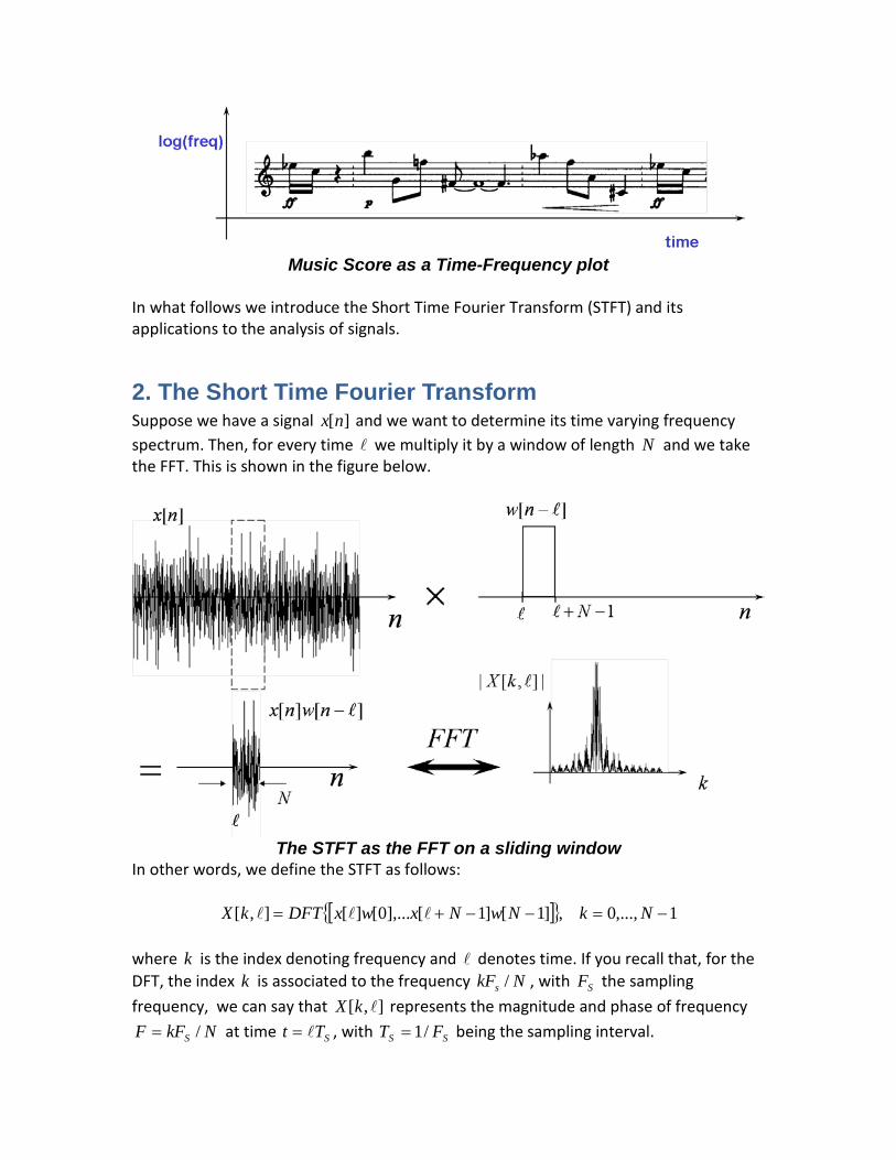
2. The Short Time Fourier Transform Suppose we have a signal ][nx and we want to determine its time varying frequency spectrum. Then, for every time we multiply it by a window of length N and we take the FFT. This is shown in the figure below.

The STFT as the FFT on a sliding window

In other words, we define the STFT as follows:

[ ]{ } 1,...,0,]1[]1[],...0[][],[ −=−−+= NkNwNxwxDFTkX

where k is the index denoting frequency and denotes time. If you recall that, for the DFT, the index k is associated to the frequency NkFs / , with SF the sampling frequency, we can say that ],[ kX represents the magnitude and phase of frequency

NkFF S /= at time STt = , with SS FT /1= being the sampling interval.

Most of the time we are interested in the magnitude ],[ kX of the STFT. Since

],[ kX is a function of two variables (time and frequency indices), its plot is three dimensional and often it is represented as an image by associating the value to an intensity level or a color. We will be giving several examples in the later part of this section. What is important to understand is what ideally we would like to see in the STFT and what in practice we can actually see. Since it is basically an application of the DFT, it presents the same issues associated to the artifacts due to the window function, such as the main lobe and sidelobes. Ideally we would like to have what is shown in the figure below.

Ideal Time Frequency Plot

In this example we see a signal with two sinusoids, one of frequency 1ω for time 0nn ≤ and one of frequency 2ω for time 0nn > . The ideal Time Frequency plot should be as shown in the figure, zero everywhere part from 21 ,ωωω = at the respective times. This would yield perfect resolution in frequency, since we see only the exact frequency, and perfect resolution in time, since we see exactly when the frequency changes. In practice, as expected, we don’t get this. As we have with the DFT, the fact that we take a window of data of length N affects the frequency resolution: the longer the window N , the better we can resolve two adjacent frequencies. However a longer window length N is going to give more uncertainty on the time the signal changes . This leads to what is called the “uncertainty principle” in Signal Processing, in the sense that we cannot resolve a signal both in time and frequency.

In the next section we address the problem of estimating the Time Frequency evolution of a signal and the effects due to finite datalength and the kind of window which we use.

3. The Spectrogram

VIDEO: Spectrogram (20:19) http://faculty.nps.edu/rcristi/eo3404/b-discrete-fourier-transform/videos/chapter3-

seg1_media/chapter3-seg1-1.wmv

The plot of the magnitude of the STFT is called the spectrogram, and that is what we get in most Signal Processing packages such as Matlab. Recall from the previous chapter that the DFT has artifacts due to the finite window length. Then the actual (non ideal) spectrogram is as shown in the figure below.

Actual Time Frequency Plot

In this figure we show two cross sections of the three dimensional plot. Each one displays the magnitude of the DFT in terms of the mainlobe and the sidelobes, for each frequency component. In particular we see that the width of the mainlobe defines the resolution in digital frequency, as

Nm πω 2

=∆

with the coefficient m depending on the window used. A rectangular window yields 2=m while the hamming, hanning, Bartlett windows have 4=m . This yields a

resolution in frequency as

NF

mF S=∆

With SF the sampling frequency. The resolution in time is given by the window length N and therefore is given by

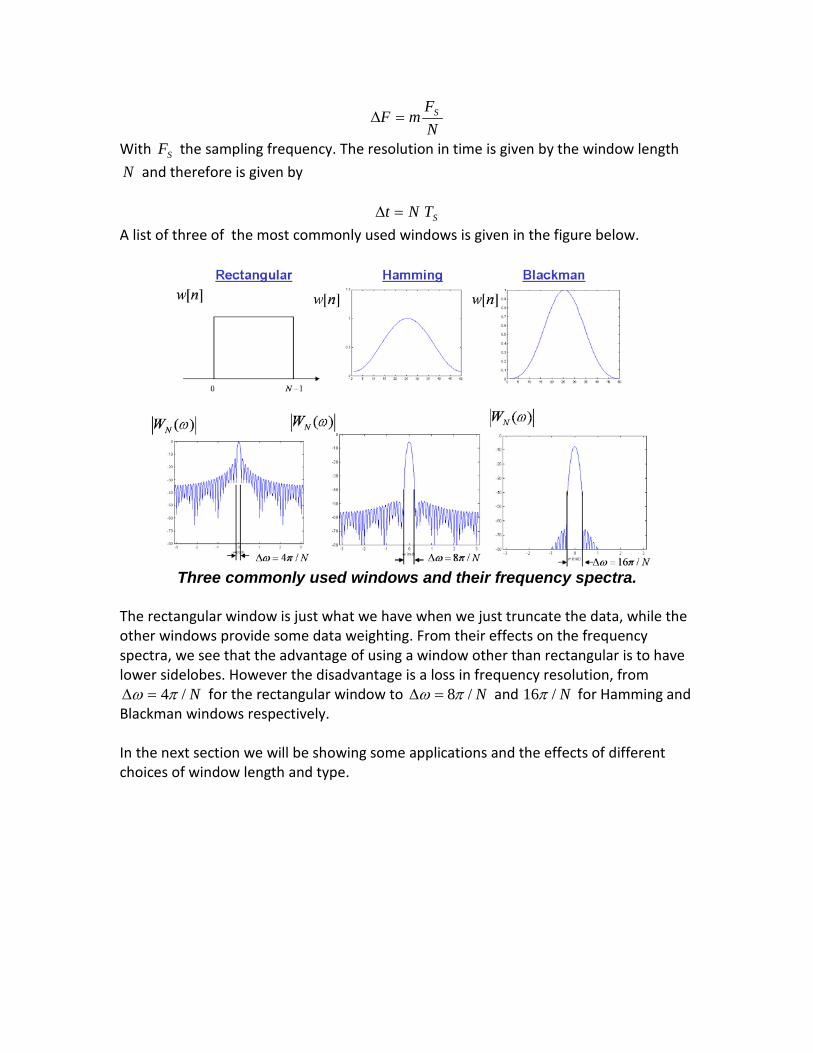
STNt =∆ A list of three of the most commonly used windows is given in the figure below.

Three commonly used windows and their frequency spectra.

The rectangular window is just what we have when we just truncate the data, while the other windows provide some data weighting. From their effects on the frequency spectra, we see that the advantage of using a window other than rectangular is to have lower sidelobes. However the disadvantage is a loss in frequency resolution, from

N/4πω =∆ for the rectangular window to N/8πω =∆ and N/16π for Hamming and Blackman windows respectively. In the next section we will be showing some applications and the effects of different choices of window length and type.

4. Examples of Applications.

4.1 Chirp signal (click here) http://faculty.nps.edu/rcristi/eo3404/b-discrete-fourier-transform/slides/chirp.wav

VIDEO: Example: Chirp (12:35)

http://faculty.nps.edu/rcristi/eo3404/b-discrete-fourier-transform/videos/chapter3-seg1_media/chapter3-seg1-2.wmv

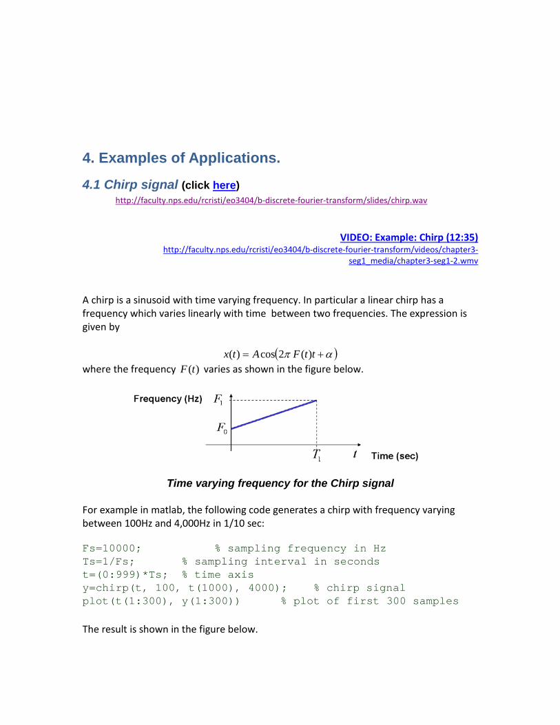
A chirp is a sinusoid with time varying frequency. In particular a linear chirp has a frequency which varies linearly with time between two frequencies. The expression is given by

( )απ += ttFAtx )(2cos)( where the frequency )(tF varies as shown in the figure below.

Time varying frequency for the Chirp signal For example in matlab, the following code generates a chirp with frequency varying between 100Hz and 4,000Hz in 1/10 sec: Fs=10000; % sampling frequency in Hz Ts=1/Fs; % sampling interval in seconds t=(0:999)*Ts; % time axis y=chirp(t, 100, t(1000), 4000); % chirp signal plot(t(1:300), y(1:300)) % plot of first 300 samples The result is shown in the figure below.

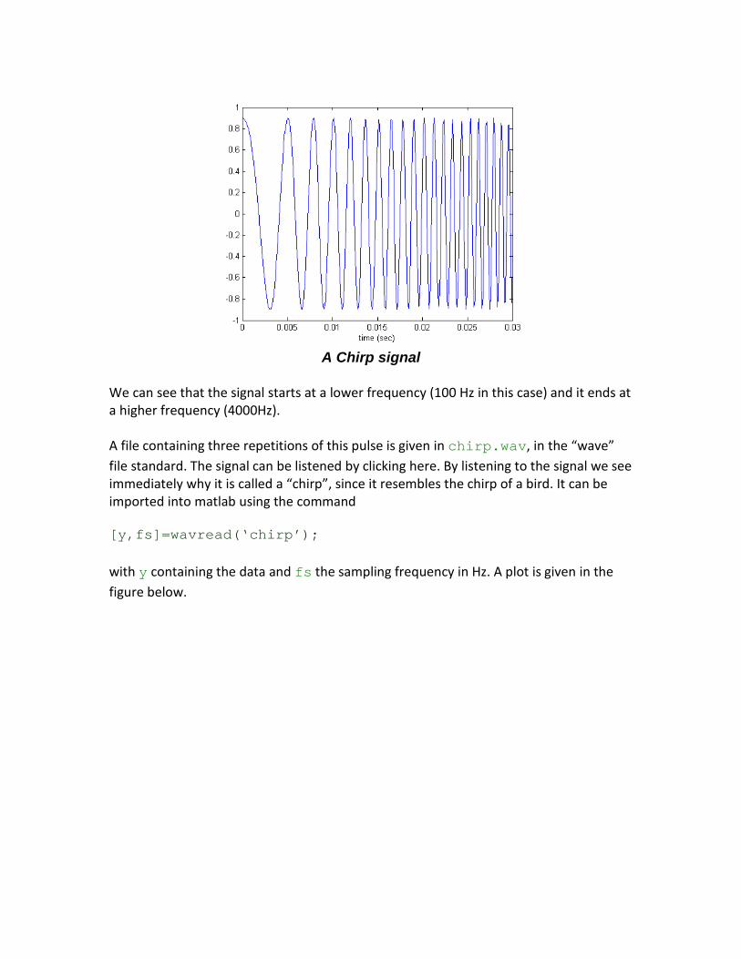
A Chirp signal

We can see that the signal starts at a lower frequency (100 Hz in this case) and it ends at a higher frequency (4000Hz). A file containing three repetitions of this pulse is given in chirp.wav, in the “wave” file standard. The signal can be listened by clicking here. By listening to the signal we see immediately why it is called a “chirp”, since it resembles the chirp of a bird. It can be imported into matlab using the command [y,fs]=wavread(‘chirp’); with y containing the data and fs the sampling frequency in Hz. A plot is given in the figure below.

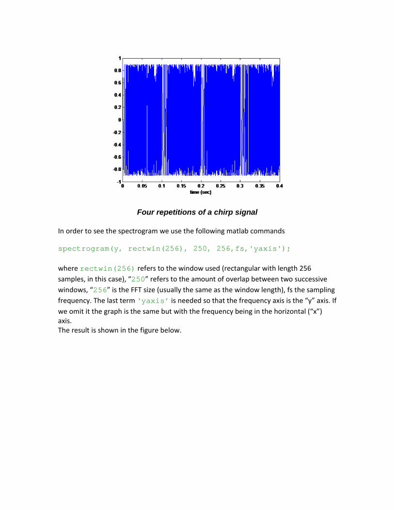
Four repetitions of a chirp signal In order to see the spectrogram we use the following matlab commands spectrogram(y, rectwin(256), 250, 256,fs,'yaxis'); where rectwin(256) refers to the window used (rectangular with length 256 samples, in this case), “250” refers to the amount of overlap between two successive windows, “256” is the FFT size (usually the same as the window length), fs the sampling frequency. The last term ‘yaxis’ is needed so that the frequency axis is the “y” axis. If we omit it the graph is the same but with the frequency being in the horizontal (“x”) axis. The result is shown in the figure below.

Spectrogram of chirp with rectangular window of length N=256

It is fairly clear from the second repetition that the frequency starts at around 100Hz, as expected and it ends at 4000Hz. In this plot we can see that, outside the actual frequencies of the signal there is quite a large amount of artifacts due to the sidelobes of the rectangular window. As expected, the use of a better window, such as the hamming window, yields a better solution. The code (just replace the window) spectrogram(y, hamming(256), 250, 256,fs,'yaxis'); yields the spectrogram shown below.

Spectrogram of chirp with hamming window of length N=256

The lower sidelobes are evident. They can be made even lower by the use of the Blackman window as spectrogram(y, blackman(256), 250, 256,fs,'yaxis'); which yields the result shown below, with even lower sidelobes.

Spectrogram of chirp with Blackman window of length N=256

The result with a shorter window, of length N=64, shows the loss in frequency resolution, but an improvement in time resolution. In fact let’s try spectrogram(y, hamming(64), 60, 64,fs,'yaxis'); and the result is shown below.

Spectrogram of chirp with hamming window of length 64 and fft size of the

same length N=64 samples

The result looks very “blocky” since we compute nly 64 frequencies. In this case it would beneficial to use a larger fft size, say N=256, as follows: spectrogram(y, hamming(64), 60, 256,fs,'yaxis'); The result is shown below, where we see the effect of using more frequencies. The window is the same, hamming of length 64 points, but in the fft it is padded with zeros up to a length N=256 to increase the number of frequencies.

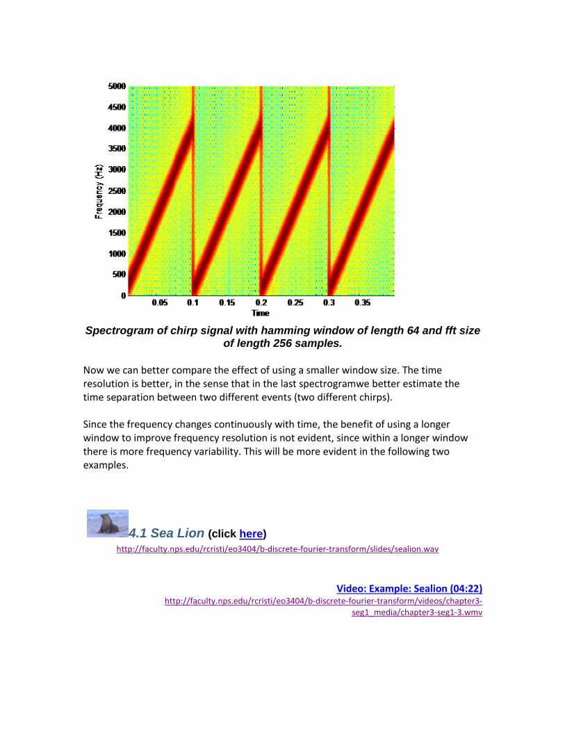
Spectrogram of chirp signal with hamming window of length 64 and fft size

of length 256 samples. Now we can better compare the effect of using a smaller window size. The time resolution is better, in the sense that in the last spectrogramwe better estimate the time separation between two different events (two different chirps). Since the frequency changes continuously with time, the benefit of using a longer window to improve frequency resolution is not evident, since within a longer window there is more frequency variability. This will be more evident in the following two examples.

4.1 Sea Lion (click here) http://faculty.nps.edu/rcristi/eo3404/b-discrete-fourier-transform/slides/sealion.wav

Video: Example: Sealion (04:22) http://faculty.nps.edu/rcristi/eo3404/b-discrete-fourier-transform/videos/chapter3-

seg1_media/chapter3-seg1-3.wmv

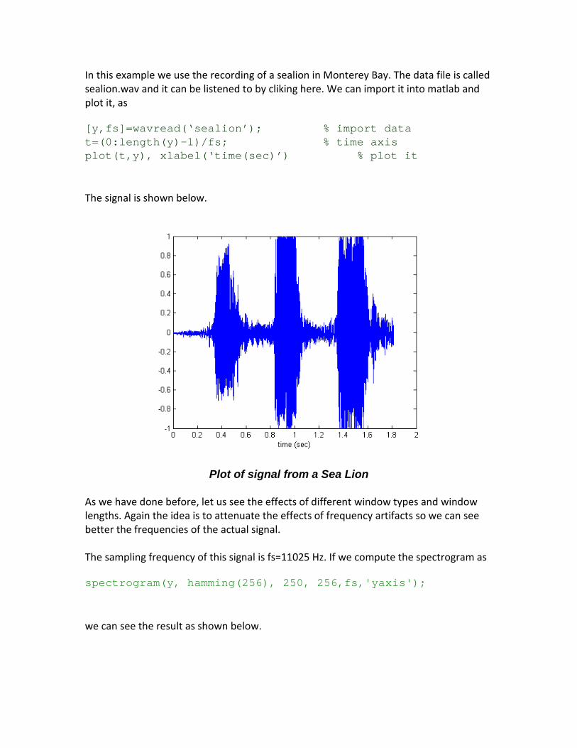
In this example we use the recording of a sealion in Monterey Bay. The data file is called sealion.wav and it can be listened to by cliking here. We can import it into matlab and plot it, as [y,fs]=wavread(‘sealion’); % import data t=(0:length(y)-1)/fs; % time axis plot(t,y), xlabel(‘time(sec)’) % plot it

The signal is shown below.

Plot of signal from a Sea Lion As we have done before, let us see the effects of different window types and window lengths. Again the idea is to attenuate the effects of frequency artifacts so we can see better the frequencies of the actual signal. The sampling frequency of this signal is fs=11025 Hz. If we compute the spectrogram as spectrogram(y, hamming(256), 250, 256,fs,'yaxis'); we can see the result as shown below.

Spectrogram of “sealion” with hamming window of length N=256

For simplicity we used only two “barks” just to illustrate the spectrum. Notice that the maximum frequency is fs/2=5012.5 Hz, as expected. Also every “bark” has a fundamental frequency (the lowest with significant amplitude) and a number of harmonics at integer multiples of the fundamental. Also the variation in time of the frequencies can be clearly associated to what we hear in the sound. Just for comparison, if we omit the window and use a rectangular window, we see a lot of artifacts as shown below (just replace “hamming” with “rectwin” in the matlab command).

Spectrogram of “sealion” with rectangular window of length 256

The presence of sidelobes is evident in this plot. Going back to using a blackman window with an increased length of N=512 samples, yields a better definition of the frequencies. This is done by the matlab command spectrogram(y, Blackman(512), 500, 512,fs,'yaxis'); which yields the figure below.

Spectrogram of “selion” with Blackman window of length N=512.

The frequencies are better defined and the sidelobes are lower.

4.3 Music Signal (click here) http://faculty.nps.edu/rcristi/eo3404/b-discrete-fourier-transform/slides/jh.wav

VIDEO: Example: Music (15:36)

http://faculty.nps.edu/rcristi/eo3404/b-discrete-fourier-transform/videos/chapter3-seg1_media/chapter3-seg1-4.wmv

In this final example we analyze a music signal. In particular we use the signal JH.wav , the opening of “Hey Joe” of Jimmy Hendrix. It can be played by clicing here. We can import it again in matlab by the wavread command and plot it as [y,fs]=wavread(‘JH’); t=(0:length(y)-1)/fs; plot(t,y), xlabel(‘time (sec)’)

The sampling frequency is fs=8000 Hz, and the signal is shown below.

Plot of the signal “JH” with respect to time.

In this example we want to address the issue of frequency resolution and the choice of window length. It is clear already from the previous example that we need to use either a hamming or a Blackman window. The Blackman window yields lower sidelobes but the price paid is a lower frequency resolution (ie wider mainlobe), so that a hamming window usually is a good compromise between low sidelobes and good frequency resolution. In the case of music we want to be able to recognize different musical notes, so to associate the musical score with the notes played by the artist. Whether you are musical or not, you can still follow the arguments in terms of signal processing. If, in addition, you have a musical talent, I am sure this example wil enable you to explore how matlab and a bit of signal rocessng can help you in discovering the “secrets” of great performances. Each musical note is associated to a frequency. In an octave there are seven notes and five half notes for a total of twelve equally frequencies. In the “A4” standard (just look at “Wikipedia” under “musical notes”) the note A in the 4th octave has a frequency of 440Hz. The note A in a different octave is obtained by dividing or multiplying the frequency by 2. So that A in the third octave has a frequency of 220 Hz. The notes of interest in this example are the ones given in the table below:

C Db D Eb E F Gb G Ab A Bb B

262 277 294 311 330 349 370 392 415 440 466 494

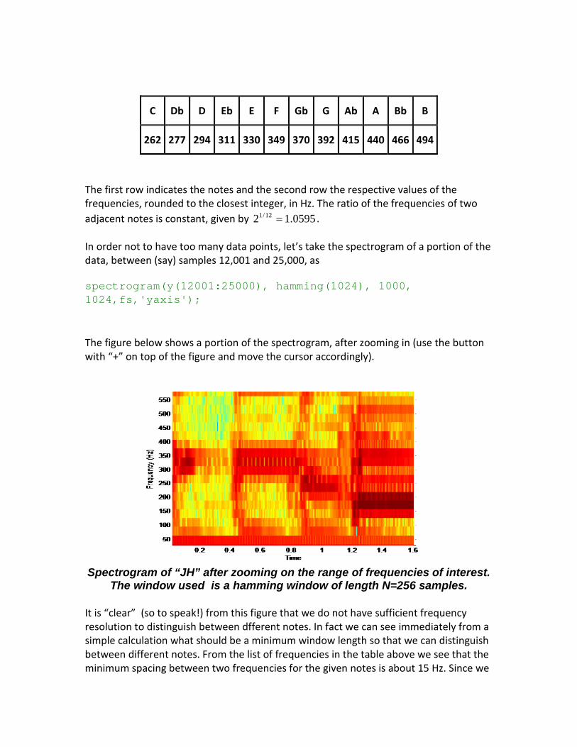
The first row indicates the notes and the second row the respective values of the frequencies, rounded to the closest integer, in Hz. The ratio of the frequencies of two adjacent notes is constant, given by 0595.12 12/1 = . In order not to have too many data points, let’s take the spectrogram of a portion of the data, between (say) samples 12,001 and 25,000, as spectrogram(y(12001:25000), hamming(1024), 1000, 1024,fs,'yaxis'); The figure below shows a portion of the spectrogram, after zooming in (use the button with “+” on top of the figure and move the cursor accordingly).

Spectrogram of “JH” after zooming on the range of frequencies of interest.

The window used is a hamming window of length N=256 samples. It is “clear” (so to speak!) from this figure that we do not have sufficient frequency resolution to distinguish between dfferent notes. In fact we can see immediately from a simple calculation what should be a minimum window length so that we can distinguish between different notes. From the list of frequencies in the table above we see that the minimum spacing between two frequencies for the given notes is about 15 Hz. Since we

use a hamming window, the frequency resolution (ie the closest frequensies we can separate) has to be smaller than 15Hz and is given by

2 15SFF HzN

∆ = ≤

Since the sampling frequency is HzFS 8000= and we want the window length N to be a power of 2, we see that a choice 1024=N is barely satisfactory (as a matter of fact it should be slightly longer, but the power of 2 is important). With this value we have the spectrogram shown below.

Spectrogram of ‘JH’ with hamming window of length N=1024 samples.

In this case we see the frequencies better defined. First notice that the fundamentals are up to about 500Hz and anything above this range is a harmonic. In what follows, let us try to see what are the frequencies so that we can compare the spectrogram with the actual score of the music. Again, you do not need to be a professional musician to follow te arguments, but just recall maybe from a lower school education some rudimentary music notation.

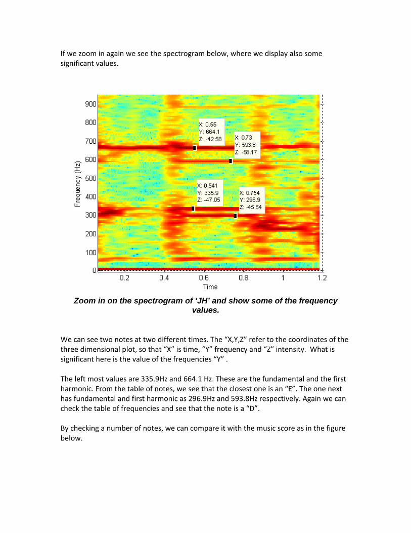
If we zoom in again we see the spectrogram below, where we display also some significant values.

Zoom in on the spectrogram of ‘JH’ and show some of the frequency

values. We can see two notes at two different times. The “X,Y,Z” refer to the coordinates of the three dimensional plot, so that “X” is time, “Y” frequency and “Z” intensity. What is significant here is the value of the frequencies “Y” . The left most values are 335.9Hz and 664.1 Hz. These are the fundamental and the first harmonic. From the table of notes, we see that the closest one is an “E”. The one next has fundamental and first harmonic as 296.9Hz and 593.8Hz respectively. Again we can check the table of frequencies and see that the note is a “D”. By checking a number of notes, we can compare it with the music score as in the figure below.

Music score and spectrogram of “JH”. Compare the three groops of notes

with the respective frequencies. In the first group we see a short (grace) “D” (there is a “natural” sign in the music score which can be missed) and an “E”. In the second we see a “D” and an “E” together, while in the third we see a short (grace note) “B” and an “A”. In all three cases note how the first harmonics follow as expected.

5. Matlab Implementation of the Spectrogram

Video: Matlab Implementation of the SSpectrogram In this section we address the matlab implementation of the spectrogram. This is on video only and the subjects presented as the following:

• WAV files http://faculty.nps.edu/rcristi/eo3404/b-discrete-fourier-transform/videos/chapter3-seg2_media/chapter3-seg2-0.wmv

• Spectrogram: Chirp http://faculty.nps.edu/rcristi/eo3404/b-discrete-fourier-transform/videos/chapter3-seg2_media/chapter3-seg2-1.wmv

• Spectrogram: Sealion

http://faculty.nps.edu/rcristi/eo3404/b-discrete-fourier-transform/videos/chapter3-seg2_media/chapter3-seg2-2.wmv

• Spectrogram: Music http://faculty.nps.edu/rcristi/eo3404/b-discrete-fourier-transform/videos/chapter3-seg2_media/chapter3-seg2-3.wmv