APPLICATION OF SHORT TIME FOURIER TRANSFORM (STFT) IN

POWER QUALITY MONITORING AND EVENT CLASSIFICATION

BY

BINOD KACHHEPATI

B.E.C.E

A thesis submitted to the Graduate School

in partial fulllment of the requirements

for the degree

Master of Science

Major Subject: Electrical Engineering

New Mexico State University

Las Cruces, New Mexico

December 2016

Application of Short Time Fourier Transform (STFT) in Power Quality Monitor-

ing and Event Classication, a thesis prepared by Binod Kachhepati in partial

fulllment of the requirements for the degree, Master of Science, has been ap-

proved and accepted by the following:

Loui ReyesDean of the Graduate School

Laura BoucheronChair of the Examining Committee

Date

Committee in charge:

Dr. Laura Boucheron, Chair

Dr. Sukumar Brahma

Dr. Huiping Cao

ii

DEDICATION

I would like to dedicate my thesis work to my beloved family and friends. A

very special feeling of gratitude to my loving parents, Gopal kachhepati and Bi-

jayashowree Kachhepati and my sisters and brother, Brinda Kachhepati, Binita

Kachhepati and Santosh Kachhepati whose words of constant encouragement and

motivation gave me all the strength to complete this work. Also, I would like to

dedicate this work to my little nephew and niece, Rounak and Aavha who always

brings smile on my face. I would also like to dedicate my work to my friends

who supported me throughout my Masters. I will always appreciate all they have

done.

iii

ACKNOWLEDGMENTS

I would like to thank my committee members who were more than generous

with their expertise and precious time. A special thanks to Dr. Laura Boucheron,

my advisor for her guidance, motivation, humbleness, support and most of all her

patience during the entire process, whose insight and experience is vital in this

work. I would also like to thank my committee members Dr. Sukumar Brahma

and Dr. Huiping Cao for agreeing to serve on my committee.

Special thanks to the Klipsch School of Electrical and Computer Engineering

Department for providing me the teaching assistant funds.

iv

VITA

December 06, 1988 Born in Bhaktapur, Nepal

2008-2011 B.E.E.C.E., Tribhuvan University,Kathmandu, Nepal

2011-2013 Service Engineer, Medical Supplies and Sales Pvt. Ltd.Kathmandu, Nepal.

2013-2014 Assistant Service Manager, Capital EnterprisesKathmandu, Nepal.

2015-Present Graduate Teaching Assistant,Electrical and Computer Engineering Department,New Mexico State University, Las Cruces, New Mexico.

FIELD OF STUDY

Major Field: Digital Signal Processing and Power System

v

ABSTRACT

APPLICATION OF SHORT TIME FOURIER TRANSFORM (STFT) IN

POWER QUALITY MONITORING AND EVENT CLASSIFICATION

BY

Binod Kachhepati

MASTER OF SCIENCE

New Mexico State University

Las Cruces, New Mexico, 2016

Dr. Laura E. Boucheron, Chair

Electrical power is the most essential raw material used by the industry and

end user/customer. The perfect power supply needs to be always available, and

within specied voltage range and frequency tolerances, and should consist of

pure and noise-free sinusoidal voltage waveforms. The study of power quality

(PQ) addresses these issues in obtaining perfect power supply. PQ is the measure

of system reliability, equipment security, and power availability in the electrical

power system. PQ has become a major concern recently because of increasing use

of sensitive devices along with restructuring of the electric power industry and

small scale distributed generation, putting more stringent demand on the qual-

ity of the electric power being supplied. Degradation in PQ is normally caused

vi

by power-line disturbances that cause malfunctions, instabilities, short lifetime,

failure of electrical equipment, etc. To improve PQ, the sources and causes of

PQ disturbances/events must be known prior to taking appropriate mitigating

actions. However, to determine the causes and sources of PQ disturbances, it is

important to detect, localize, and classify them. This thesis explores a theoretical

framework based on the Short Time Fourier Transform (STFT) for two important

applications. The rst application provides a comprehensive study of the imple-

mentation of STFT in PQ monitoring for identication and event classication.

The STFT tool is implemented in detecting and localizing seven dierent types

of PQ disturbances in a simulation framework. The feature vector thus extracted

from the STFT matrix, when fed to the k Nearest Neighbor (k-NN) and Sup-

port Vector Machine (SVM) classiers, is found to be capable of classifying the

multi-class PQ disturbances even in the presence of noise. The second applica-

tion explores two important problems in a renewable rich electric power system

- harmonic analysis and fault detection. The theoretical STFT tool, based on a

time-frequency transform is shown to be promising in measuring time varying har-

monics over a wide range, and distinguishing between two dynamic events, fault

and capacitor switching, by analyzing the inverter output current. In particular,

a limited set of window lengths provides harmonic analysis accuracy competitive

with the more computationally demanding S-transform.

vii

CONTENTS

LIST OF TABLES . . . . . . . . . . . . . . . . . . . . . . . . . . . . . xi

LIST OF FIGURES . . . . . . . . . . . . . . . . . . . . . . . . . . . . xiii

1 INTRODUCTION . . . . . . . . . . . . . . . . . . . . . . . . . . 1

1.1 Power Quality and Eects of Disturbances to Power Quality . . . 1

1.2 Importance of Identication and Classication of PQ Disturbances 3

1.3 Diculties in Classication of PQ Disurbances . . . . . . . . . . . 4

1.4 Problem Denition . . . . . . . . . . . . . . . . . . . . . . . . . . 6

1.5 Thesis layout . . . . . . . . . . . . . . . . . . . . . . . . . . . . . 7

2 LITERATURE REVIEW . . . . . . . . . . . . . . . . . . . . . . 9

2.1 PQ Studies . . . . . . . . . . . . . . . . . . . . . . . . . . . . . . 9

2.2 Detection Methods . . . . . . . . . . . . . . . . . . . . . . . . . . 9

2.3 Classication Methods . . . . . . . . . . . . . . . . . . . . . . . . 11

3 POWER QUALITY DISTURBANCES . . . . . . . . . . . . . . . 14

3.1 Types of PQ Problems . . . . . . . . . . . . . . . . . . . . . . . . 14

3.2 Various Power Quality Disturbances . . . . . . . . . . . . . . . . . 15

3.2.1 Sags (Dips) . . . . . . . . . . . . . . . . . . . . . . . . . . 15

3.2.2 Swell . . . . . . . . . . . . . . . . . . . . . . . . . . . . . . 17

3.2.3 Harmonics . . . . . . . . . . . . . . . . . . . . . . . . . . . 17

3.2.4 Interharmonics . . . . . . . . . . . . . . . . . . . . . . . . 19

3.2.5 Flicker . . . . . . . . . . . . . . . . . . . . . . . . . . . . . 20

3.2.6 Interruption . . . . . . . . . . . . . . . . . . . . . . . . . . 20

3.2.7 Notch . . . . . . . . . . . . . . . . . . . . . . . . . . . . . 22

viii

3.2.8 Transients . . . . . . . . . . . . . . . . . . . . . . . . . . . 22

3.3 Harmonics and Problems in Identifying Disturbances in Renewable

Rich Electric Power Systems . . . . . . . . . . . . . . . . . . . . . 23

4 POWER QUALITY MONITORING . . . . . . . . . . . . . . . . 26

4.1 Detection Process . . . . . . . . . . . . . . . . . . . . . . . . . . . 27

4.2 Signal Analysis . . . . . . . . . . . . . . . . . . . . . . . . . . . . 27

4.3 Disturbance Characterization . . . . . . . . . . . . . . . . . . . . 29

4.4 Power Quality Standards . . . . . . . . . . . . . . . . . . . . . . . 31

5 TIME FREQUENCY REPRESENTATION . . . . . . . . . . . . 32

5.1 Time Frequency Analysis . . . . . . . . . . . . . . . . . . . . . . 32

5.2 Discrete Fourier Transform . . . . . . . . . . . . . . . . . . . . . . 34

5.3 Discrete Short Time Fourier Transform . . . . . . . . . . . . . . 35

5.3.1 Time Frequency Resolution Trade-o . . . . . . . . . . . . 38

5.3.2 Spectral Peak Correction in Discrete STFT . . . . . . . . . 39

5.3.3 Amplitude and Phase Correction in STFT . . . . . . . . . 41

6 METHODOLOGY . . . . . . . . . . . . . . . . . . . . . . . . . . 42

6.1 Proposed Method for PQ Monitoring in Identication and Event

Classication Using STFT Framework . . . . . . . . . . . . . . . 42

6.1.1 Pre-processing . . . . . . . . . . . . . . . . . . . . . . . . . 42

6.1.2 Feature Extraction . . . . . . . . . . . . . . . . . . . . . . 43

6.1.3 Classication . . . . . . . . . . . . . . . . . . . . . . . . . 43

6.2 Proposed Method for PQ Monitoring for Renewables Rich Electric

Power Systems . . . . . . . . . . . . . . . . . . . . . . . . . . . . 45

7 EXPERIMENTAL RESULTS . . . . . . . . . . . . . . . . . . . . 47

7.1 Data Generation for PQ Analysis . . . . . . . . . . . . . . . . . . 47

ix

21 Falling degree of voltge sag and interruption . . . . . . . . . . . . 58

22 Feature 5 versus Feature 1 scatterplot. . . . . . . . . . . . . . . . 61

23 Feature 2 versus Feature 5 scatterplot. . . . . . . . . . . . . . . . 62

24 Feature 4 versus Feature 5 scatterplot. . . . . . . . . . . . . . . . 62

25 3D feature plot (Feature 1, 2 and 5 scatterplot). . . . . . . . . . . 63

26 Estimation of best window size of harmonic components . . . . . 74

27 Estimation of best window size for interharmonic components . . 75

28 Harmonic components in a signal . . . . . . . . . . . . . . . . . . 76

29 Estimated amplitude of harmonic components . . . . . . . . . . . 78

30 Estimated phase of harmonic components . . . . . . . . . . . . . 79

31 Interharmonic components in a signal . . . . . . . . . . . . . . . . 81

32 Estimated amplitude of interharmonic components . . . . . . . . 83

33 Discriminating among two dynamic events . . . . . . . . . . . . . 85

xiii

1 INTRODUCTION

Traditional power system structures have changed in recent years, and the elec-

trical power system can no longer be viewed as a single entity. The conventional

way of transporting electric power via transmission networks which is unidirec-

tional from generators to end users or customers, is now not adequate for current

deregulated systems [1].

An electrical power system is always expected to provide undistorted sinusoidal

rated voltage and current continuously at a rated frequency to every end user

connected in the system. However, the proliferation of power electronics-based

controllers and devices along with restructuring of the electric power industry and

small-scale distributed generation have increasingly put more stringent demand

on the quality of electric power supplied [2]- [4].

1.1 Power Quality and Eects of Disturbances to Power Quality

Power Quality (PQ) is a consumer-driven issue and hence can be best dened as

any power problem manifested in the voltage, current and/or frequency devia-

tions that result in the failure or misoperation of customers' equipment [5]. The

highest PQ is achieved when voltage and current have purely sinusoidal waveforms

containing only the power frequency and when the voltage magnitude corresponds

to its reference value. The best measure of PQ is the ability of electrical equipment

to function in a satisfactory manner without any adverse eects to the normal op-

eration of other equipment connected to the system.

PQ has become a signicant issue for both the utility and customers. In

1

early days, power quality issues were concerned with power system transients

due to switching and lightning surges, induction furnaces, and other cyclic loads.

The increase of highly sensitive computerized systems, complex interconnection

of systems, widespread use of power electronics devices, embedded generation

and renewable energy resources, and fast control schemes used in electrical power

networks have been driving factors for the interest in PQ and demand for PQ has

resulted in many PQ issues and problems [6].

Most often a disturbance in voltage also causes a disturbance in the current

and hence the term PQ is used when referring to both voltage quality or current

quality. Degradation in the quality of electric power is normally caused by power-

line disturbances such as voltage sag, swell, momentary interruption, harmonic

distortion, icker, notch, spike, and transients [7]. These degradations, even when

momentary in nature, can cause problems such as malfunctions, instabilities, short

lifetime, failure of electrical equipment, and hours of manufacturing downtime for

industries.

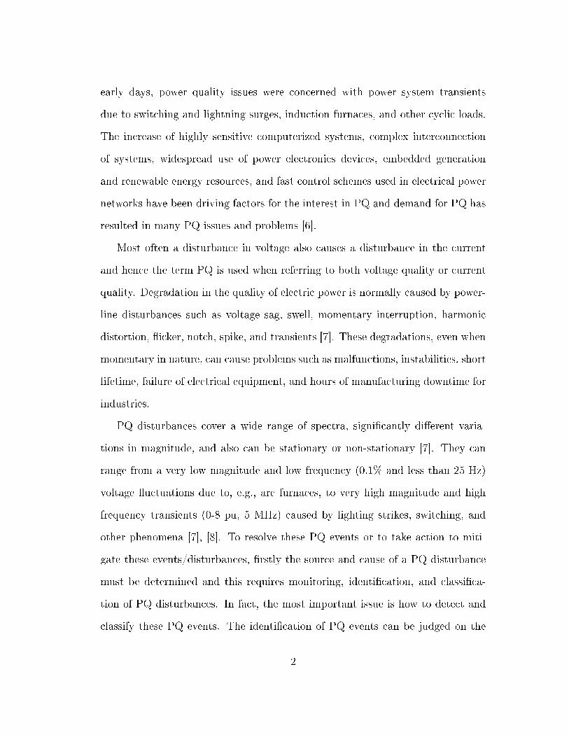
PQ disturbances cover a wide range of spectra, signicantly dierent varia-

tions in magnitude, and also can be stationary or non-stationary [7]. They can

range from a very low magnitude and low frequency (0.1% and less than 25 Hz)

voltage uctuations due to, e.g., arc furnaces, to very high magnitude and high

frequency transients (0-8 pu, 5 MHz) caused by lighting strikes, switching, and

other phenomena [7], [8]. To resolve these PQ events or to take action to miti-

gate these events/disturbances, rstly the source and cause of a PQ disturbance

must be determined and this requires monitoring, identication, and classica-

tion of PQ disturbances. In fact, the most important issue is how to detect and

classify these PQ events. The identication of PQ events can be judged on the

2

basis of information regarding typical magnitude, duration, and spectral content

for each category of an event and comparison to specications of the Institute

of Electrical and Electronics Engineers (IEEE) and International Electrotechnical

Commission (IEC) standards [1], [9], [10]. The detection based on inspection of

the disturbance waveform by human operators is laborious, time consuming and

inaccurate. Hence, PQ monitoring should be an integral part of overall system

performance assessment procedures.

1.2 Importance of Identication and Classication of PQ Disturbances

The increased connection and widespread use of power electronics devices with

sensitive and fast control schemes in electrical networks have brought many tech-

nical and economic advantages, but they have also caused degradation of PQ.

There are various reasons for the deterioration of the power quality. The main

reasons for the growing interest in PQ problems are summarized as follows:

• Modern electric appliances are equipped with power electronics devices that

are built on microprocessor/microcontroller architectures. These appliances

introduce various types of PQ disturbances.

• Complex interconnected systems result in more severe consequences if any

of the connected components fail. Moreover, sophisticated power electronics

equipment, which is very sensitive to PQ disturbances, are used for improv-

ing system stability, operation, and eciency.

• Industrial equipment such as high-eciency, adjustable speed motor drives

and shunt capacitors are now extensively used. The complexity of industrial

processes results in huge economic losses if equipment fails or malfunctions.

3

• There has been a signicant increase in renewable energy sources, micro-

sources and inverter interfaced distributed energy resources (IIDERs) that

result in PQ disturbances such as voltage variations, icker, and wave-

form distortions with higher order harmonic and interharmonic components.

Moreover, inverter output current is limited to the rated current in a sub-

cycle time frame, which appears similar for faults and other disturbances

like capacitor switching, and these disturbances also have high frequency

transients at the onset of each event, thus making it hard to detect and

distinguish between these disturbances.

To maintain a reasonable level of power quality, the identication and classi-

cation of PQ disturbances causing a particular PQ problem are necessary. The

ability to locate the sources of that disturbance in the power system is also im-

portant so that necessary corrective action can be taken to mitigate the prob-

lems promptly. The detection and analysis of interharmonics and supraharmonics

associated with IIDERs has been particularly dicult with existing monitoring

systems. There is thus much interest in adaptation of existing or development of

new techniques capable of analyzing interharmonics and supraharmonics.

1.3 Diculties in Classication of PQ Disurbances

The complexity of PQ problems and the lack of reliable techniques for analyzing

these problems have hindered power utilities' ability to maintain the required level

of power quality without considerable increase in cost. Accurate PQ disturbance

classication, which depends on the several factors, is a dicult task. The fol-

lowing are the some of the major issues and challenges in the classication of PQ

disturbances.

4

• Classier performance is highly dependent on the extracted features of the

disturbance signal. Dening eective features for classifying PQ distur-

bances is a dicult task, especially when a new disturbances such as har-

monics, interharmonics, and supraharmonics are introduced. This thesis

focuses on application of the Short Time Fourier Transform (STFT) specif-

ically to analyze harmonics, interharmonics, and supraharmonics.

• An important concern is the number of decomposition levels required in

wavelet analysis to avoid loss of important information and to have an ac-

curate classier since PQ disturbances cover a wide range of frequencies.

This thesis focuses on application of the STFT with a limited set of window

lengths to cover a wide range of PQ monitoring and analysis applications.

• Noise present in the signal caused by control circuits, loads with solid-state

rectiers, switching power supplies, and power electronics devices [1], has

been a major issue in accurate feature extraction and classication of PQ

events. This thesis studies the eect of noise on PQ event classication.

• Most studies have trained and tested on synthetic data. A comprehen-

sive standard PQ database for testing and comparison of state of the art

techniques is also needed. Due to the diculties in acquiring real-world

disturbance measurements and accurate modeling of a real-world power sys-

tem, this thesis generates synthetic signals from parametric equations for

the study of the signal processing methods.

5

1.4 Problem Denition

The increase in occurrence and variety of PQ disturbances and the impact to end

users/customers necessitates the development of signal processing tools to moni-

tor and analyze PQ disturbances. A good monitoring system should incorporate

detection capabilities into the monitoring so that events of interest can be rec-

ognized and captured automatically. Recently, to detect, localize, and classify

PQ disturbances, researchers have focused on signal processing techniques to de-

compose power signals into a set of features from where decision making becomes

easier and more accurate than conventional methods of visual inspection [11]-

[14]. The majority of signal processing methods reported in the literature utilize

time, frequency, and time-frequency domain representations of the PQ distur-

bance waveform, on the basis of which many specic features are derived in order

to classify dierent types of PQ disturbances.

With the increasing usage of renewable energy resources (wind and solar) and

micro-sources (fuel cells and micro-turbine), IIDERs have become important com-

ponents in power systems nowadays. Therefore, there is also a need to monitor

these renewable-rich power systems. The broadband spectrum of power invert-

ers [15]- [17] and interconnection of IIDERs to the power system generate sig-

nicant higher order harmonic and interharmonic components. There is a much

required need to accurately measure these kind of harmonics and interharmonics.

The most dicult problem faced by today's PQ disturbance classication

method is the large variation in the morphology of PQ disturbance waveforms.

Thus, in order to handle the practical situations of real-life applications as men-

tioned above, development of a method with an eective feature set for PQ distur-

bance classication that is capable of providing performance with greater accuracy

6

with simplicity in computation is indeed a dicult problem.

1.5 Thesis layout

The layout of this thesis is as follows.

Chapter 1 has provided an introduction to power quality particularly as it

applies to current changes in power system. It has also summarized PQ problems,

the importance for identifying and classifying the PQ events/disturbances, the

associated diculties in classifying PQ problems and problems in a renewable

rich power system.

Chapter 2 provides a literature review on PQ studies and then briey reviews

the state-of-the-art in PQ identication and classication.

Chapter 3 provides details on types of PQ problems, various PQ disturbances

considered in this thesis, associated diculties in measuring time varying har-

monics and problems in identifying disturbances in renewable rich electric power

systems.

Chapter 4 elaborates on PQ monitoring and its signicance in the electrical

power system. The detection process, various signal processing methods imple-

mented for the signal analysis, and some widely used characterization for PQ

disturbances are discussed in detail. PQ standards currently used are discussed

briey.

Chapter 5 discusses how time-frequency analysis can be implemented to iden-

tify dierent non-stationary signals. Dierent types of time-frequency analysis

including limitations of the Discrete Fourier Transform (DFT) are discussed. The

discrete Short Time Fourier Transform (STFT) is then introduced and its ap-

plication in PQ monitoring, the time-frequency resolution problem inherited by

7

the STFT, spectral peak correction, and correction for amplitude and phase are

discussed.

Chapter 6 explains the proposed methodology used in the thesis. The rst part

proposes a combination of an STFT framework and k- Nearest Neighbor (k-NN)

along with Support Vector Machine (SVM) classiers for the identication and

classication of dierent types of PQ disturbances in PQ monitoring. The second

part proposes a real-time monitoring strategy based on the theoretical framework

of the STFT focusing mainly on the renewable rich electric power system.

Chapter 7 provides the experimental analysis and results from the research

work. The rst section of this chapter explains the seven dierent PQ distur-

bance signals generated for the analysis and study. Mathematical models are

used in simulating these PQ disturbance signals. Details regarding the feature

extraction using the STFT and the classication results from the two classiers

are presented. The second section then estimates the amplitudes and phases of

time varying harmonic and interharmonic components, including supraharmonic

components, for monitoring the renewable rich electric power system. Also, results

for distinguishing among two dynamic events are presented.

Chapter 8 summarizes the research work and Chapter 9 provides insight into

the future work and improvements that can be done to this work.

8

2 LITERATURE REVIEW

This chapter provides a literature review on PQ studies. It also briey reviews

the state of the art in PQ identication and classication.

2.1 PQ Studies

The degradation in quality of electric power due to various disturbances has be-

come a major concern nowadays. References [18]- [20] provide various guidelines

regarding monitoring PQ disturbances. A basic introduction to various PQ distur-

bances possible in a power distribution scenario is provided in [19]. [18] provides a

survey of various distribution sites and concluded various interesting observations

about the various disturbance occurrence statistics which includes statistics that

the majority of the voltage sags have a magnitude of around 80% and a dura-

tion of around 4 to 10 cycles and that the total harmonic distortion on harmonic

disturbances is around 1.5 times the normal value.

2.2 Detection Methods

Since PQ disturbance signals are non-stationary, the general methods of frequency

analysis are not satisfactory for classication purposes. Therefore, many signal

processing techniques have been utilized to extract features from a PQ disturbance

signal based on the time-frequency domain and then use dierent classiers for

classication.

One of the most widely used tools in signal processing is Fourier analysis [21].

The Fourier transform is very useful in the analysis of harmonics. However, there

9

are some disadvantages, such as losses of temporal information, so that it can only

be used in the steady state.

Time frequency information related to voltage disturbance waveforms can be

obtained using the Short Time Fourier Transform (STFT) [22]. The STFT as

a time-frequency analysis technique depends critically on the choice of the win-

dow. In [11], the discrete STFT is used for the time-frequency domain whereas

a dyadic and binary-tree wavelet lter is used for time-scale domain for analysis

of voltage disturbances, particularly voltage sags. Dyadic wavelet lters are not

suitable for harmonic analysis of disturbance data as the lter center frequencies

and bandwidths are inexible [11]. The band-pass lter outputs from the discrete

STFT are more suitable for time-frequency domain analysis of harmonic related

voltage disturbances. The STFT method is also compared to wavelet transform

(WT) in [11]. The choice of these methods depends heavily on the particular

applications [11]. By selecting a small window length, discrete STFT is able to

detect and analyze transient change at voltage sag-initiation and at voltage recov-

ery. Overall it appears more favorable to use discrete STFT than dyadic wavelet

and binary-tree wavelet lters for voltage disturbance analysis [11].

Wavelet transforms (WTs) are widely used for disturbance detection in PQ

recently [23]- [24]. Wavelets have been very useful in electrical transient analysis.

Papers [25]- [29] present the properties of WTs and their use in scenarios simi-

lar to power quality disturbance classication. Paper [25] applies wavelet models

to model several short term events like a capacitor switching transient, an au-

toreclosure, and a voltage dip. Paper [26] uses continuous wavelet transform to

detect and analyze voltage sags and transients. Paper [27] present unique features

to characterize three common power quality events at the distribution level and

10

methodologies to extract them using Fourier and wavelet transforms, the Fourier

transform characterizes the steady state phenomena, and the wavelet transform

is applied to the transient phenomena. An event identication module is then

built by utilizing these characteristics [27]. Paper [28] implements WT and de-

tects various transient events and it then integrates the WT with the probabilistic

network (PNN) model and classify those events. The classied accuracy rate was

90% with more training examples in consideration [28]. Paper [29] uses a WT for

on-line voltage disturbance detection where the WT was faster and more precise

in discriminating transient events than the conventional detection approach based

on voltage transformation to a synchronously rotating frame.

The S-transform introduced in [30] is used to analyze PQ disturbances in [13],

[31]- [34]. An S-Transform based intelligent system in [32] is proposed for classi-

cation of power quality disturbance signals, where the classication accuracy was

found very high (94% from the feedforward network and 92.67% from the PNN)

and was practically invariant to noise, showing S-transform's robustness. In [34],

a comparison between the WT and S-transform for PQ disturbance recognition is

provided, where the S-transform showed good computational scalability and very

low sensitivity to noise levels during the classications.

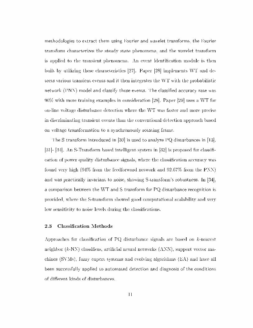
2.3 Classication Methods

Approaches for classication of PQ disturbance signals are based on k-nearest

neighbor (k-NN) classiers, articial neural networks (ANN), support vector ma-

chines (SVMs), fuzzy expert systems and evolving algorithms (EA) and have all

been successfully applied to automated detection and diagnosis of the conditions

of dierent kinds of disturbances.

11

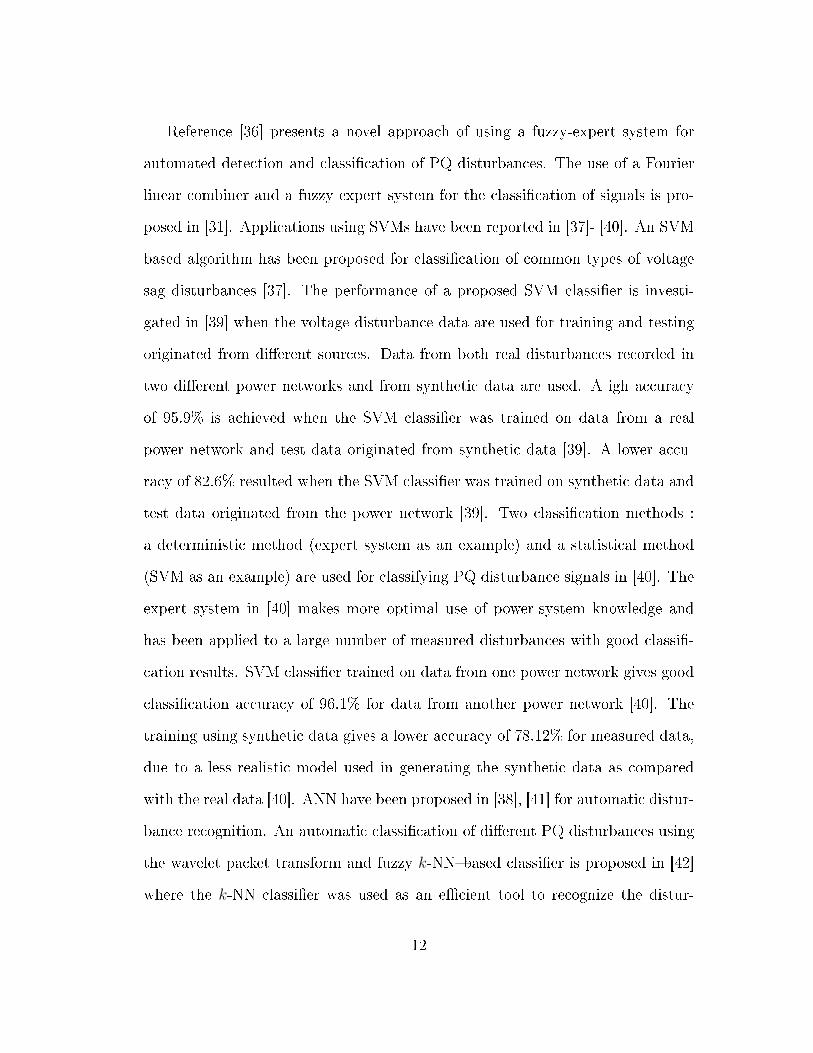
Reference [36] presents a novel approach of using a fuzzy-expert system for

automated detection and classication of PQ disturbances. The use of a Fourier

linear combiner and a fuzzy expert system for the classication of signals is pro-

posed in [31]. Applications using SVMs have been reported in [37]- [40]. An SVM

based algorithm has been proposed for classication of common types of voltage

sag disturbances [37]. The performance of a proposed SVM classier is investi-

gated in [39] when the voltage disturbance data are used for training and testing

originated from dierent sources. Data from both real disturbances recorded in

two dierent power networks and from synthetic data are used. A igh accuracy

of 95.9% is achieved when the SVM classier was trained on data from a real

power network and test data originated from synthetic data [39]. A lower accu-

racy of 82.6% resulted when the SVM classier was trained on synthetic data and

test data originated from the power network [39]. Two classication methods :

a deterministic method (expert system as an example) and a statistical method

(SVM as an example) are used for classifying PQ disturbance signals in [40]. The

expert system in [40] makes more optimal use of power-system knowledge and

has been applied to a large number of measured disturbances with good classi-

cation results. SVM classier trained on data from one power network gives good

classication accuracy of 96.1% for data from another power network [40]. The

training using synthetic data gives a lower accuracy of 78.12% for measured data,

due to a less realistic model used in generating the synthetic data as compared

with the real data [40]. ANN have been proposed in [38], [41] for automatic distur-

bance recognition. An automatic classication of dierent PQ disturbances using

the wavelet packet transform and fuzzy k-NNbased classier is proposed in [42]

where the k-NN classier was used as an ecient tool to recognize the distur-

12

bances at particular point of time, and the classier provided a good classication

accuracy of 93.7% with the optimal feature vector used. In [43], a multi-label

classication predicted the classes of multiple disturbances for a power quality

(PQ) event, classied them eectively with good accuracy of 96.27%.

13

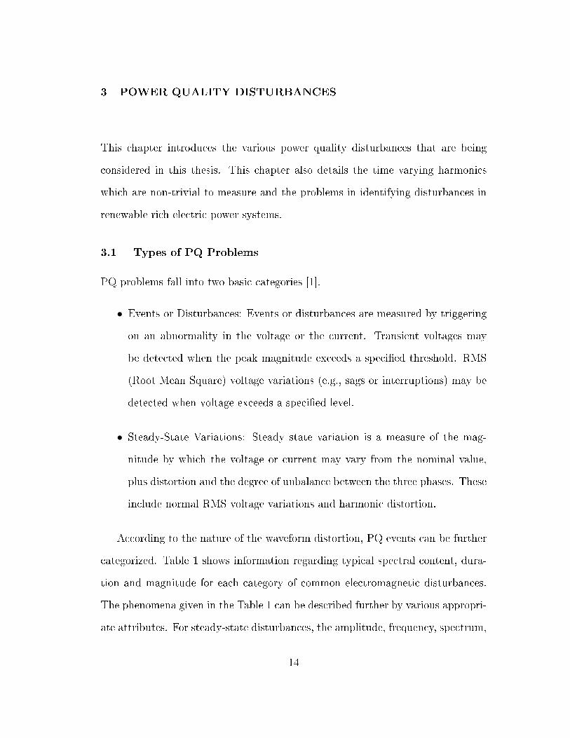
3 POWER QUALITY DISTURBANCES

This chapter introduces the various power quality disturbances that are being

considered in this thesis. This chapter also details the time varying harmonics

which are non-trivial to measure and the problems in identifying disturbances in

renewable rich electric power systems.

3.1 Types of PQ Problems

PQ problems fall into two basic categories [1].

• Events or Disturbances: Events or disturbances are measured by triggering

on an abnormality in the voltage or the current. Transient voltages may

be detected when the peak magnitude exceeds a specied threshold. RMS

(Root Mean Square) voltage variations (e.g., sags or interruptions) may be

detected when voltage exceeds a specied level.

• Steady-State Variations: Steady state variation is a measure of the mag-

nitude by which the voltage or current may vary from the nominal value,

plus distortion and the degree of unbalance between the three phases. These

include normal RMS voltage variations and harmonic distortion.

According to the nature of the waveform distortion, PQ events can be further

categorized. Table 1 shows information regarding typical spectral content, dura-

tion and magnitude for each category of common electromagnetic disturbances.

The phenomena given in the Table 1 can be described further by various appropri-

ate attributes. For steady-state disturbances, the amplitude, frequency, spectrum,

14

modulation, source impedance, notch depth, and notch area attributes can be uti-

lized whereas attributes like rate of rise, rate of occurrence, and energy potential

are useful for non-steady state disturbances [44].

3.2 Various Power Quality Disturbances

PQ disturbances are usually characterized in terms of the eect to the system

voltage and supply frequency. They can be broadly classied according to volt-

age magnitude variations, frequency variations and transients. The denitions

according to IEEE standard 1159-2009 [1] and summarized in Table 1 are given in

the following sections. Some usual causes of these disturbances and their negative

eects to the power system [1] are also discussed.

The example waveforms shown in the following sections are generated from

parametric equation-based simulation of various PQ events; further details about

the simulation and PQ disturbance signals are provided in Chapter 6.

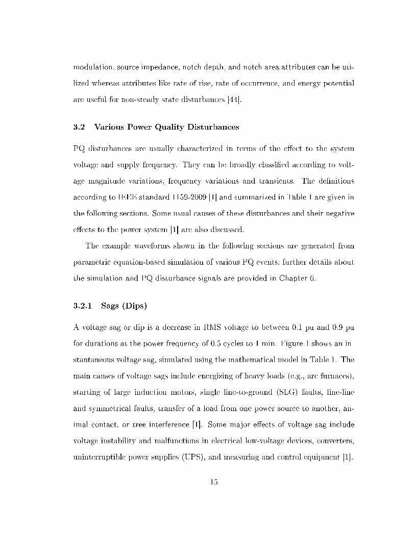
3.2.1 Sags (Dips)

A voltage sag or dip is a decrease in RMS voltage to between 0.1 pu and 0.9 pu

for durations at the power frequency of 0.5 cycles to 1 min. Figure 1 shows an in-

stantaneous voltage sag, simulated using the mathematical model in Table 1. The

main causes of voltage sags include energizing of heavy loads (e.g., arc furnaces),

starting of large induction motors, single line-to-ground (SLG) faults, line-line

and symmetrical faults, transfer of a load from one power source to another, an-

imal contact, or tree interference [1]. Some major eects of voltage sag include

voltage instability and malfunctions in electrical low-voltage devices, converters,

uninterruptible power supplies (UPS), and measuring and control equipment [1].

15

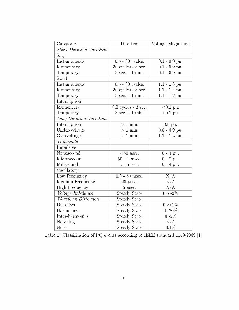
Categories Duration Voltage MagnitudeShort Duration Variation

SagInstantaneous 0.5 - 30 cycles. 0.1 - 0.9 pu.Momentary 30 cycles - 3 sec. 0.1 - 0.9 pu.Temporary 3 sec. - 1 min. 0.1 - 0.9 pu.SwellInstantaneous 0.5 - 30 cycles. 1.1 - 1.8 pu.Momentary 30 cycles - 3 sec. 1.1 - 1.4 pu.Temporary 3 sec. - 1 min. 1.1 - 1.2 pu.InterruptionMomentary 0.5 cycles - 3 sec. <0.1 pu.Temporary 3 sec. - 1 min. <0.1 pu.Long Duration Variation

Interruption > 1 min. 0.0 pu.Under-voltage > 1 min. 0.8 - 0.9 pu.Overvoltage > 1 min. 1.1 - 1.2 pu.Transients

ImpulsiveNanosecond <50 nsec. 0 - 4 pu.Microsecond 50 - 1 msec. 0 - 8 pu.Milisecond >1 msec. 0 - 4 pu.OscillatoryLow Frequency 0.3 - 50 msec. N/AMedium Frequency 20 µsec. N/AHigh Frequency 5 µsec. N/AVoltage Imbalance Steady State 0.5 -2%Waveform Distortion Steady StateDC oset Steady State 0 -0.1%Harmonics Steady State 0 -20%Inter-harmonics Steady State 0 -2%Notching Steady State N/ANoise Steady State 0.1%

Table 1: Classication of PQ events according to IEEE standard 1159-2009 [1]

16

0 0.02 0.04 0.06 0.08 0.1 0.12 0.14 0.16 0.18 0.2−1.5

−1

−0.5

0

0.5

1

1.5

Time sec)

Am

plitu

de p

u

Figure 1: Instantaneous voltage sag.

Also, problems in interfacing with communication signals can arise. Lights may

dim briey. More sensitive equipment could be more noticeably aected.

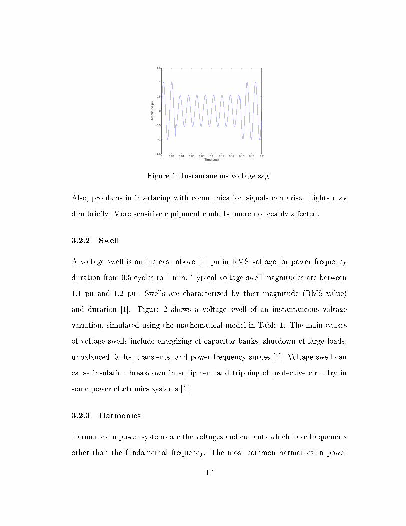
3.2.2 Swell

A voltage swell is an increase above 1.1 pu in RMS voltage for power frequency

duration from 0.5 cycles to 1 min. Typical voltage swell magnitudes are between

1.1 pu and 1.2 pu. Swells are characterized by their magnitude (RMS value)

and duration [1]. Figure 2 shows a voltage swell of an instantaneous voltage

variation, simulated using the mathematical model in Table 1. The main causes

of voltage swells include energizing of capacitor banks, shutdown of large loads,

unbalanced faults, transients, and power frequency surges [1]. Voltage swell can

cause insulation breakdown in equipment and tripping of protective circuitry in

some power electronics systems [1].

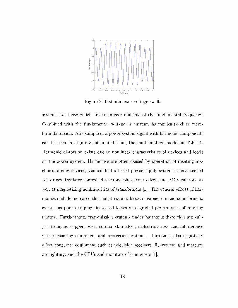
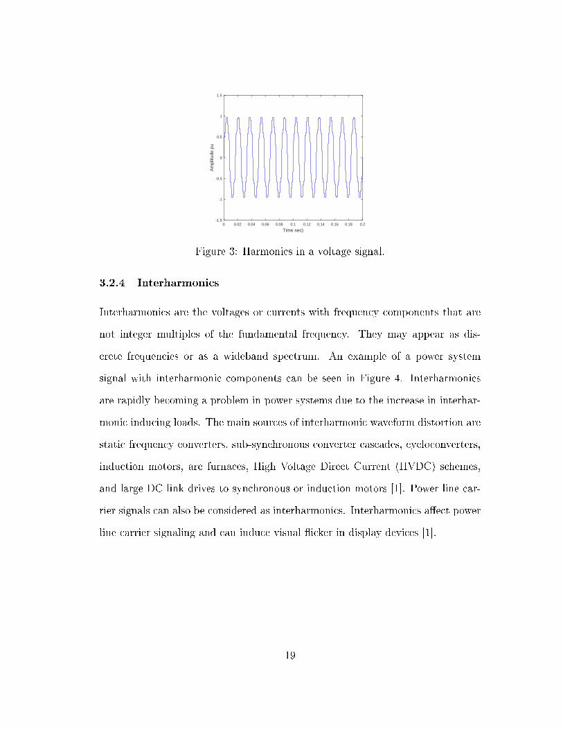
3.2.3 Harmonics

Harmonics in power systems are the voltages and currents which have frequencies

other than the fundamental frequency. The most common harmonics in power

17

Time sec)0 0.02 0.04 0.06 0.08 0.1 0.12 0.14 0.16 0.18 0.2

Am

plitu

de p

u-1.5

-1

-0.5

0

0.5

1

1.5

Figure 2: Instantaneous voltage swell.

systems are those which are an integer multiple of the fundamental frequency.

Combined with the fundamental voltage or current, harmonics produce wave-

form distortion. An example of a power system signal with harmonic components

can be seen in Figure 3, simulated using the mathematical model in Table 1.

Harmonic distortion exists due to nonlinear characteristics of devices and loads

on the power system. Harmonics are often caused by operation of rotating ma-

chines, arcing devices, semiconductor based power supply systems, converter-fed

AC drives, thyristor controlled reactors, phase controllers, and AC regulators, as

well as magnetizing nonlinearities of transformers [1]. The general eects of har-

monics include increased thermal stress and losses in capacitors and transformers,

as well as poor damping, increased losses or degraded performance of rotating

motors. Furthermore, transmission systems under harmonic distortion are sub-

ject to higher copper losses, corona, skin eect, dielectric stress, and interference

with measuring equipment and protection systems. Harmonics also negatively

aect consumer equipment such as television receivers, uorescent and mercury

arc lighting, and the CPUs and monitors of computers [1].

18

Time sec)0 0.02 0.04 0.06 0.08 0.1 0.12 0.14 0.16 0.18 0.2

Am

plitu

de p

u

-1.5

-1

-0.5

0

0.5

1

1.5

Figure 3: Harmonics in a voltage signal.

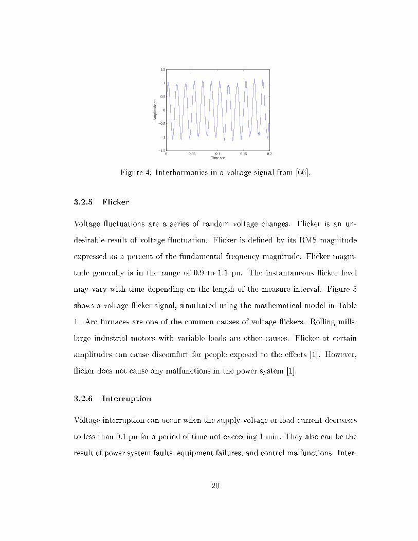
3.2.4 Interharmonics

Interharmonics are the voltages or currents with frequency components that are

not integer multiples of the fundamental frequency. They may appear as dis-

crete frequencies or as a wideband spectrum. An example of a power system

signal with interharmonic components can be seen in Figure 4. Interharmonics

are rapidly becoming a problem in power systems due to the increase in interhar-

monic inducing loads. The main sources of interharmonic waveform distortion are

static frequency converters, sub-synchronous converter cascades, cycloconverters,

induction motors, arc furnaces, High Voltage Direct Current (HVDC) schemes,

and large DC link drives to synchronous or induction motors [1]. Power line car-

rier signals can also be considered as interharmonics. Interharmonics aect power

line carrier signaling and can induce visual icker in display devices [1].

19

0 0.05 0.1 0.15 0.2−1.5

−1

−0.5

0

0.5

1

1.5

Time secA

mpl

itude

pu

Figure 4: Interharmonics in a voltage signal from [66].

3.2.5 Flicker

Voltage uctuations are a series of random voltage changes. Flicker is an un-

desirable result of voltage uctuation. Flicker is dened by its RMS magnitude

expressed as a percent of the fundamental frequency magnitude. Flicker magni-

tude generally is in the range of 0.9 to 1.1 pu. The instantaneous icker level

may vary with time depending on the length of the measure interval. Figure 5

shows a voltage icker signal, simultated using the mathematical model in Table

1. Arc furnaces are one of the common causes of voltage ickers. Rolling mills,

large industrial motors with variable loads are other causes. Flicker at certain

amplitudes can cause discomfort for people exposed to the eects [1]. However,

icker does not cause any malfunctions in the power system [1].

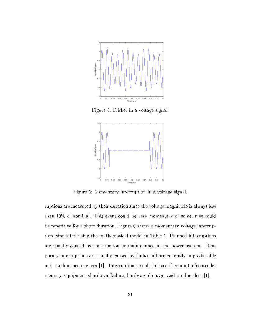
3.2.6 Interruption

Voltage interruption can occur when the supply voltage or load current decreases

to less than 0.1 pu for a period of time not exceeding 1 min. They also can be the

result of power system faults, equipment failures, and control malfunctions. Inter-

20

Time sec)0 0.02 0.04 0.06 0.08 0.1 0.12 0.14 0.16 0.18 0.2

Am

plitu

de p

u-1.5

-1

-0.5

0

0.5

1

1.5

Figure 5: Flicker in a voltage signal.

Time sec)0 0.02 0.04 0.06 0.08 0.1 0.12 0.14 0.16 0.18 0.2

Am

plitu

de p

u

-1.5

-1

-0.5

0

0.5

1

1.5

Figure 6: Momentary interruption in a voltage signal.

ruptions are measured by their duration since the voltage magnitude is always less

than 10% of nominal. This event could be very momentary or sometimes could

be repetitive for a short duration. Figure 6 shows a momentary voltage interrup-

tion, simulated using the mathematical model in Table 1. Planned interruptions

are usually caused by construction or maintenance in the power system. Tem-

porary interruptions are usually caused by faults and are generally unpredictable

and random occurrences [1]. Interruptions result in loss of computer/controller

memory, equipment shutdown/failure, hardware damage, and product loss [1].

21

Time sec0 0.01 0.02 0.03 0.04 0.05 0.06 0.07 0.08

Am

plitu

de p

u-1.5

-1

-0.5

0

0.5

1

1.5

Figure 7: Notches in a voltage signal.

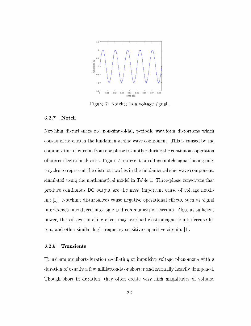
3.2.7 Notch

Notching disturbances are non-sinusoidal, periodic waveform distortions which

consist of notches in the fundamental sine wave component. This is caused by the

commutation of current from one phase to another during the continuous operation

of power electronic devices. Figure 7 represents a voltage notch signal having only

5 cycles to represent the distinct notches in the fundamental sine wave component,

simulated using the mathematical model in Table 1. Three-phase converters that

produce continuous DC output are the most important cause of voltage notch-

ing [1]. Notching disturbances cause negative operational eects, such as signal

interference introduced into logic and communication circuits. Also, at sucient

power, the voltage notching eect may overload electromagnetic interference l-

ters, and other similar high-frequency sensitive capacitive circuits [1].

3.2.8 Transients

Transients are short-duration oscillating or impulsive voltage phenomena with a

duration of usually a few milliseconds or shorter and normally heavily dampened.

Though short in duration, they often create very high magnitudes of voltage.

22

Time sec0 0.02 0.04 0.06 0.08 0.1 0.12 0.14 0.16 0.18 0.2

Am

plitu

de p

u-1.5

-1

-0.5

0

0.5

1

1.5

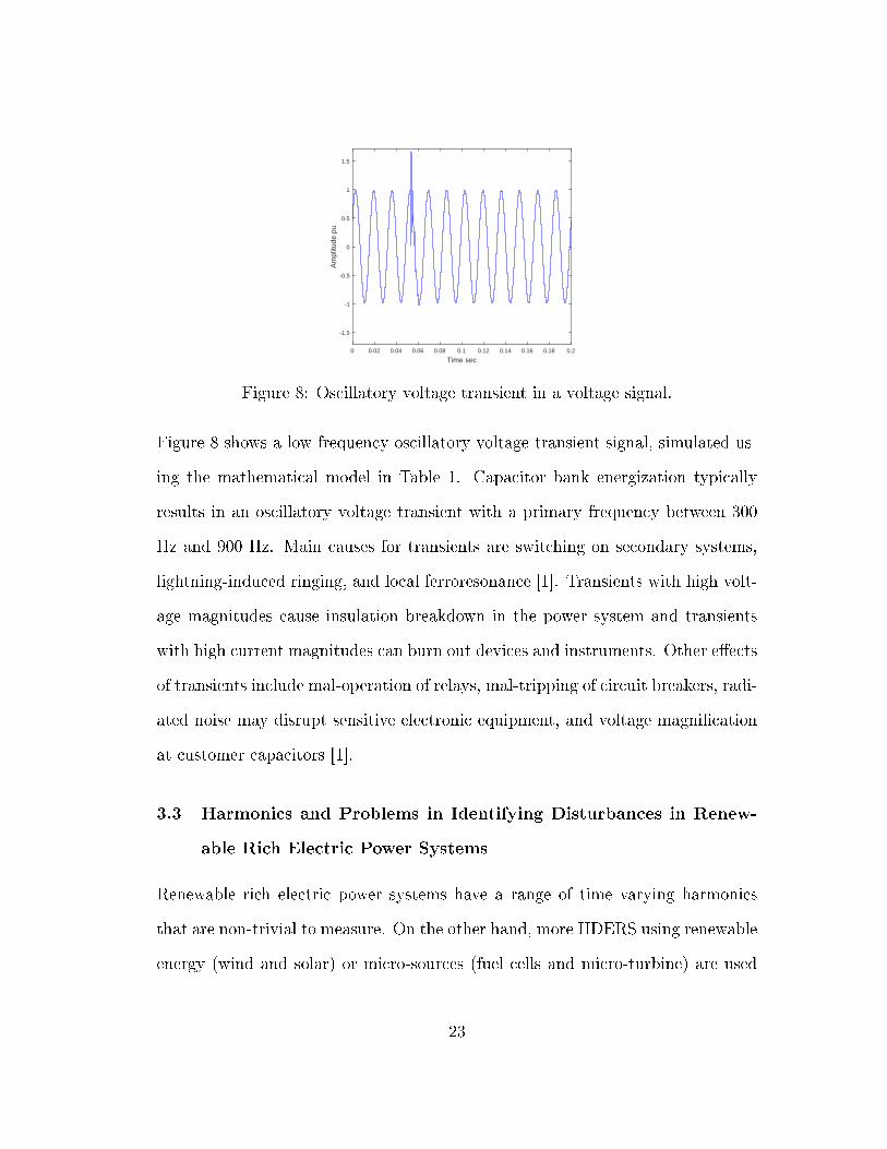
Figure 8: Oscillatory voltage transient in a voltage signal.

Figure 8 shows a low-frequency oscillatory voltage transient signal, simulated us-

ing the mathematical model in Table 1. Capacitor bank energization typically

results in an oscillatory voltage transient with a primary frequency between 300

Hz and 900 Hz. Main causes for transients are switching on secondary systems,

lightning-induced ringing, and local ferroresonance [1]. Transients with high volt-

age magnitudes cause insulation breakdown in the power system and transients

with high current magnitudes can burn out devices and instruments. Other eects

of transients include mal-operation of relays, mal-tripping of circuit breakers, radi-

ated noise may disrupt sensitive electronic equipment, and voltage magnication

at customer capacitors [1].

3.3 Harmonics and Problems in Identifying Disturbances in Renew-

able Rich Electric Power Systems

Renewable rich electric power systems have a range of time varying harmonics

that are non-trivial to measure. On the other hand, more IIDERS using renewable

energy (wind and solar) or micro-sources (fuel cells and micro-turbine) are used

23

nowadays and also several other nonlinear loads connected to power systems have

impacts on the stability of the system.

Common sources of harmonics include nonlinear loads, saturable devices and

power electronics devices [45]. As the power systems grid continually changes,

new phenomena related to traditional power systems harmonics are being intro-

duced. As intermodulation between the fundamental and the harmonic compo-

nents of a system occur, a component with a frequency of a non-integer multiple

can occur [46]. Interharmonics are rapidly becoming a problem in power systems

because of a drastic increase in loads inducing interharmonics. The broadband

spectrum of power inverters used in power systems comprising renewable energy

sources generate signicant higher order harmonic and interharmonic components.

Supra-harmonics, the harmonics in the 2-150 kHz range, are presently of high in-

terest for two reasons; 1) there is a lack of standards (emission, immunity and

compatibility) [48]- [50] and 2) frequencies within this range are used for auto-

mated meter reading (9 to 95 kHz) [47]. There is a much required need to develop

a signal processing technique to accurately measure these kind of harmonics [47].

Narrow band components in the supraharmonics are not stationary and change

amplitude over time. The emission can also have other features like time-frequency

variations which are not common in the harmonic range [48], [49] and thus need

joint time-frequency analysis rather than traditional Fourier analysis [51].

Inverter response to disturbances has been a major operational issue. IIDERs'

output current is limited to the rated current in a sub cycle time frame which

creates a dicult scenario for fault detection for any protective device installed

at point of interconnection (POI) of such DERs. The sudden switching of large

loads or a capacitor in distribution feeders will also result in similar rise in currents.

24

This limitation of currents from the IIDERs create diculties in distinguishing

between the power disturbances as both of these disturbances have high frequency

transients at the onset of each event that looks similar, making it hard to identify

by traditional detection methods.

A major problem for power resources is that their response to faults is such

that they are typically fault-blinded because they are not able to detect a fault.

Additionally, they are not able to distinguish a typical fault from other dynamic

events taking place on the system. Also, nonlinear loads and power sources inject

time-varying harmonics into the system. To account for these diverse issues, a

generalized framework based on signal processing is required.

25

4 POWER QUALITY MONITORING

PQ monitoring in an electric power system is necessary to characterize dierent

PQ disturbances at a particular location in the system. PQ monitoring forms

an integral part of the overall system performance assessment procedures. Under

the deregulation of utilities, the necessity for monitoring has increased due to the

diculty in diagnosing incompatibilities between the electric power supply and

the load equipment. The need to study distortion levels at particular locations

becomes very important in order to rene modeling techniques or to develop a PQ

baseline. Monitoring the PQ can be used to predict future performance of load

equipment or PQ mitigating techniques [1]. However, preventing economic dam-

age occurring due to PQ disturbances in a critical load environment is the most

important reason for monitoring electric PQ. The frequency of PQ disturbances

and their duration aect PQ costs.

PQ monitoring is the process of collecting, analyzing, and interpreting raw

data into useful information. The process of collecting data is usually carried out

by continuous measurement of voltage and current over some extended time pe-

riod. The process of analysis and interpretation has traditionally been performed

manually. However, recent advances in signal processing techniques and articial

intelligence have made it possible to design and implement intelligent automated

systems to automatically analyze and interpret raw data, with minimal human

intervention [5].

26

4.1 Detection Process

The detection process is the rst step in PQ monitoring which deals with PQ

problems. The techniques used in the detection process are time-dependent which

require sample data to be compared with a threshold to determine start and end

points of a disturbance. The simplest detection method is to identify any deviation

of time-dependent RMS voltage/current magnitudes from the nominal waveform.

This method has been used for detecting voltage dips, swells, and interruptions

[52]- [54]. Another technique in detecting fast step changes (in voltage or current),

is to use high pass or band pass lters. A disturbance in a power system often

results in a fast step change, and also results in high-frequency oscillations. A high

pass lter can thus be used to detect such step changes or oscillations. Wavelet

lters are known to be eective in detecting multi-scale singular points and these

lters can detect the start and end points of a disturbance usually relating to the

signicant sudden changes or singularities in the signal waveform [54].

4.2 Signal Analysis

Signal analysis is the second step in PQ monitoring which involves signal process-

ing techniques to analyze the voltage and current measurements from the detected

sampled disturbance waveform. Signal processing techniques are needed for the

characterization (feature extraction) of variation and events, for the triggering

mechanism needed to detect events, and to extract additional information from

the measurements [7]. Several signal processing techniques have been used to

analye PQ disturbance signals. Some common techniques are reported below.

27

Discrete Fourier Transform (DFT)

The traditional method used to obtain the fundamental and harmonic compo-

nents of a signal is the application of the DFT to the samples of the signal taken

in a time window.

Short Time Fourier Transform (STFT)

The STFT provides a time-frequency signal decomposition, which is equivalent

to applying a set of equal-bandwidth sub-band lters. The STFT is a Fourier-

based transform used to determine the sinusoidal frequency and phase content of

local sections of a signal as they changes over time.

S- Transform

The S-transform is a time-localized Fourier spectrum and has a window whose

height and width vary unlike the STFT [30]. It can be considered an extension

of the WT [30], [34]. The S-transform has an advantage over the WT in that

it it provides multi-resolution analysis while retaining the absolute phase of each

frequency [30]- [34]. However, selecting a suitable window to match the specic

frequency content of the signal results a poor energy concentration in the time-

frequency domain: poor time resolution at lower frequencies and poor frequency

resolution at higher frequencies [30], [33], [34]. Additionally, the S-transform is

more computationally complex to implement and more complicated to interpret

than standard Fourier-based methods.

Wavelet Transform

The wavelet transform (WT) is a signicant tool for monitoring PQ problems

28

[25]- [29]. The multi-resolution capabilities of the WT distinguishes it from the

Fourier-based mentods technique. A wavelet transform using a multi-resolution

signal decomposition technique is ecient in analyzing transient events [27]. A

multi-resolution signal decomposition has the ability to detect and localize tran-

sient events and furthermore classify dierent power quality disturbances using

unique features extracted from WT for dierent power quality disturbances.

Kalman Filters

Kalman lters have been used as an alternative method to the Root Mean

Square (RMS) method to detect and analyze voltage events in power systems

[53], [55]. Unlike the RMS method [52], [54], the Kalman ltering method gives

information both on the magnitude and phase angle of the voltage supply during

an event and the time when the voltage event begins. Kalman lters are used

to estimate the time dependent signal components, magnitudes, and frequency

components using selected harmonic frequencies.

4.3 Disturbance Characterization

Disturbance characterization is the process of categorizing PQ disturbance sig-

nals into dierent types according to their extracted features. It is important to

dene and extract good-quality features in the analysis step for any successful

disturbance characterization. Articial Neural Networks (ANN), Support Vector

Machine (SVM), k- Nearest Neighbour (k-NN), Expert Systems and so on are

highlighted in this section.

Articial Neural Networks: ANNs have been an important tool for the

statistical-based categorization of power system disturbances [38], [41]. Neural

29

networks are nonlinear statistical data modeling tools. Categorization using neural

networks is a good alternative only when enough data is available.

Support Vector Machines: A Support Vector Machine (SVM) performs

classication by constructing an N-dimensional hyper-plane that optimally sepa-

rates the data into two categories. SVMs are able to nd non-linear boundaries if

classes are not linearly separable. SVM models use a kernel function to project the

features into a higher dimensional space where the data may be better separated

by a hyperplane.

k- Nearest Neighbour: The k-nearest neighbor (k-NN) classier is a method

for classication based on the closest training examples in the feature space. The

classier compares a new sample (testing data) with the baseline data (training

data) and nds the k- neighborhood in the training data and assigns the class

which appears more frequently in the k-neighborhood. Therefore, an object is

classied by a majority vote of its neighbors, with the object being assigned to

the class most common amongst its k nearest neighbors, where k is a typically

small positive integer.

Expert System: An expert system is a deterministic approach for catego-

rization. A set of rules, where the real intelligence from human experts in power

systems is translated into the articial intelligence in computers, forms the core

of an expert system [36]. The performance of categorization is directly dependent

on the set of IF-THEN rules, and the inference that performs the reasoning of

rules. The main disadvantage of an expert system is the need for predetermined

thresholds to make binary decisions, and choosing undesirable thresholds leads to

less accuracy in categorization.

The PQ monitoring process depends on power quality standards that dene

30

acceptable limits for the monitoring process. The dierent threshold limits and the

standard classication of PQ disturbance signals in PQ monitoring is useless if it is

not compared to the power quality baselines or standards. Power quality standards

dene acceptable and measurable limits of voltage, current, and deviations from

normal frequency. The main benets of PQ standards are to make clear to utilities

and customers about acceptable and unacceptable levels of service and to protect

the utility's and end user's equipment from failing or operating improperly when

PQ disturbances occur.

4.4 Power Quality Standards

There are various organizations that develop PQ standards. The Institute of Elec-

trical and Electronics Engineers (IEEE), American National Standards Institute

(ANSI), and Electric Power Research Institute (EPRI) are very famous in North

America, whereas the International Electrotechnical Commission (IEC) is a widely

known organization in Europe. Utilities and end-users/customers need standards

that set limits on electrical disturbances that their equipment can withstand and

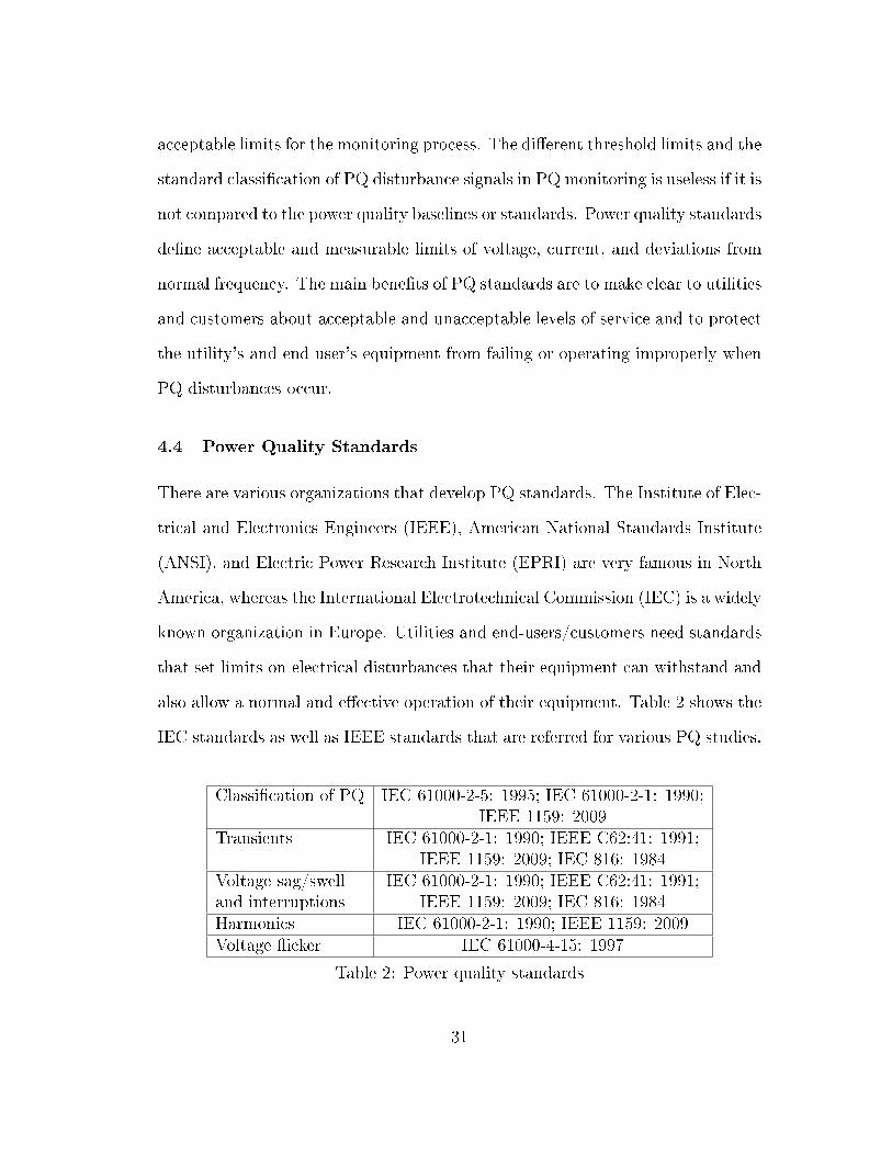
also allow a normal and eective operation of their equipment. Table 2 shows the

IEC standards as well as IEEE standards that are referred for various PQ studies.

Classication of PQ IEC 61000-2-5: 1995; IEC 61000-2-1: 1990;IEEE 1159: 2009

Transients IEC 61000-2-1: 1990; IEEE C62:41: 1991;IEEE 1159: 2009; IEC 816: 1984

Voltage sag/swell IEC 61000-2-1: 1990; IEEE C62:41: 1991;and interruptions IEEE 1159: 2009; IEC 816: 1984Harmonics IEC 61000-2-1: 1990; IEEE 1159: 2009Voltage icker IEC 61000-4-15: 1997

Table 2: Power quality standards

31

5 TIME FREQUENCY REPRESENTATION

Due to increased awareness of PQ, the need for PQ monitoring is important. PQ

monitoring forms an integral part of overall system performance assessment proce-

dures. Signal processing techniques form an important part of PQ monitoring and

analysis of voltage and current measurements from the sampled waveform. Signal

processing techniques are needed for the characterization (feature extraction) of

variation and events, for the triggering mechanism needed to detect events, and

to extract additional information from the measurements [7]. The increase in oc-

currence and variety of PQ disturbances and impact to end users/customers has

necessitated the development of signal processing tools to monitor and analyze

PQ disturbances.

Moreover, inverter response to disturbances creates a major operational issue

where the limitation imposed on the currents from the IIDERs create diculties

in identifying and discriminating between faults or sudden switching of large loads

or a capacitor in distribution feeders, making it hard to be detected by traditional

detection methods. Also, nonlinear loads and power sources inject time varying

harmonics into the system. To account for these diverse issues, a generalized

framework based on signal processing is required.

5.1 Time Frequency Analysis

Time Frequency Analysis (TFA) is a signal processing tool which has wide eld

applications particularly in extracting valuable information from non-stationary

signals [56], [57]. It combines time domain analysis and frequency domain analysis

32

to yield a potentially more revealing picture of temporal localization of a signal's

spectral components [58], [59]. Since time-frequency representations (TFR) indi-

cate variations of the spectral characteristics of the signal as a function of time,

they are ideally suited for non-stationary signals.

Non-stationary signals are signals in which frequency components are not

present at all the times in the signal. To analyze any non-stationary signal such as

a voltage or current, we need to use a multi-resolution technique which provides

the TFR. TFA techniques decompose any non-stationary signal in terms of a joint

time-frequency domain representation, which captures the time evolving contri-

bution of the frequency components present in the signal. In other words, TFA

techniques can extract instantaneous estimates of amplitude and phase change

of frequency components. Therefore, every unique type of non-stationary signal

is expected to have a unique signature in the time-frequency (TF) plane. This

property enables the TFA approach to be used as a potential tool to distinguish

among dierent types of non-stationary signals; voltages and currents are the

non-stationary signals in this study.

Techniques of TFA for non-stationary signals can generally be divided into two

categories: (1) linear transforms, which primarily include the Short-Time Fourier

Transform (STFT) and Wavelet Transform (WT), and (2) Quadratic (Bilinear)

Transforms, which mainly include the Wigner Distribution (WD) and Ambiguity

Function (AF) [60]. Linear TF transforms are preferred because of their low

computation and ease of parameter estimation in in general [44]. The discrete

STFT, which is a linear TF transform, overcomes the lack of time resolution of

the DFT by using the moving windowing technique performing Fourier analysis

of data sliced by the moving window. Although the STFT has a xed frequency

33

resolution for all frequencies once the size of the window is chosen, it enables an

easier interpretation compared to the WT in terms of harmonics and maintains

the absolute phase of each localized frequency component.

5.2 Discrete Fourier Transform

The Fourier transform is one of the most common spectral analysis techniques.

It transforms a time domain signal to a frequency domain signal, which is an

alternate representation of a signal. In most cases the frequency domain shows

certain features of the signal that were not visible in the time domain.

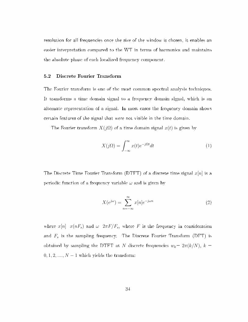
The Fourier transform X(jΩ) of a time domain signal x(t) is given by

X(jΩ) =

∫ ∞−∞

x(t)e−jΩtdt (1)

The Discrete Time Fourier Transform (DTFT) of a discrete time signal x[n] is a

periodic function of a frequency variable ω and is given by

X(ejω) =∞∑

n=−∞

x[n]e−jωn (2)

where x[n]=x(nFs) and ω=2πF/Fs, where F is the frequency in consideration

and Fs is the sampling frequency. The Discrete Fourier Transform (DFT) is

obtained by sampling the DTFT at N discrete frequencies wk= 2π(k/N), k =

0, 1, 2, ...., N − 1 which yields the transform:

34

X[k] =N−1∑n=0

x[n]e−j2πknN (3)

The DFT has some disadvantages. The DFT computes spectral content for

all integer values k, but the spectral content in between integer values must be

otherwise estimated. For non-stationary signals, the spectral content changes with

time and hence the time averaged amplitude spectrum computed using the DFT

may be inadequate to track changes. A solution to most of the above mentioned

diculties of the DFT is a TFA.

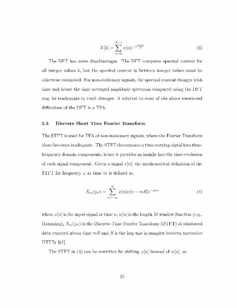
5.3 Discrete Short Time Fourier Transform

The STFT is used for TFA of non-stationary signals, where the Fourier Transform

alone becomes inadequate. The STFT decomposes a time-varying signal into time-

frequency domain components, hence it provides an insight into the time-evolution

of each signal component. Given a signal x[n], the mathematical denition of the

STFT for frequency ω at time m is dened as,

Xm(jω) =∞∑

n=−∞

x[n]w[n−mR]e−jωn (4)

where x[n] is the input signal at time n, w[n] is the lengthM window function (e.g.,

Hamming), Xm(jω) is the Discrete-Time Fourier Transform (DTFT) of windowed

data centered about time mR and R is the hop size in samples between successive

DTFTs [61].

The STFT in (4) can be rewritten by shifting x[n] instead of w[n], as

35

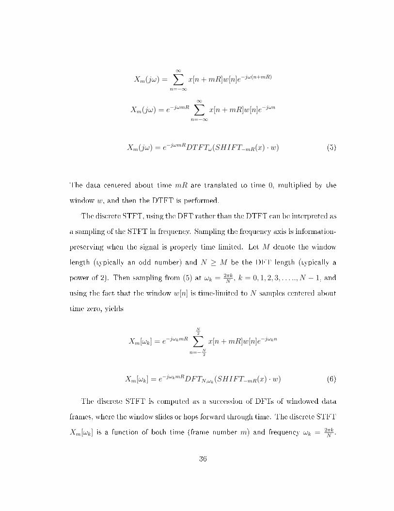
Xm(jω) =∞∑

n=−∞

x[n+mR]w[n]e−jω(n+mR)

Xm(jω) = e−jωmR∞∑

n=−∞

x[n+mR]w[n]e−jωn

Xm(jω) = e−jωmRDTFTω(SHIFT−mR(x) · w) (5)

The data centered about time mR are translated to time 0, multiplied by the

window w, and then the DTFT is performed.

The discrete STFT, using the DFT rather than the DTFT can be interpreted as

a sampling of the STFT in frequency. Sampling the frequency axis is information-

preserving when the signal is properly time limited. Let M denote the window

length (typically an odd number) and N ≥ M be the DFT length (typically a

power of 2). Then sampling from (5) at ωk = 2πkN, k = 0, 1, 2, 3, . . . .., N − 1, and

using the fact that the window w[n] is time-limited to N samples centered about

time zero, yields

Xm[ωk] = e−jωkmR

N2∑

n=−N2

x[n+mR]w[n]e−jωkn

Xm[ωk] = e−jωkmRDFTN,ωk(SHIFT−mR(x) · w) (6)

The discrete STFT is computed as a succession of DFTs of windowed data

frames, where the window slides or hops forward through time. The discrete STFT

Xm[ωk] is a function of both time (frame number m) and frequency ωk = 2πkN.

36

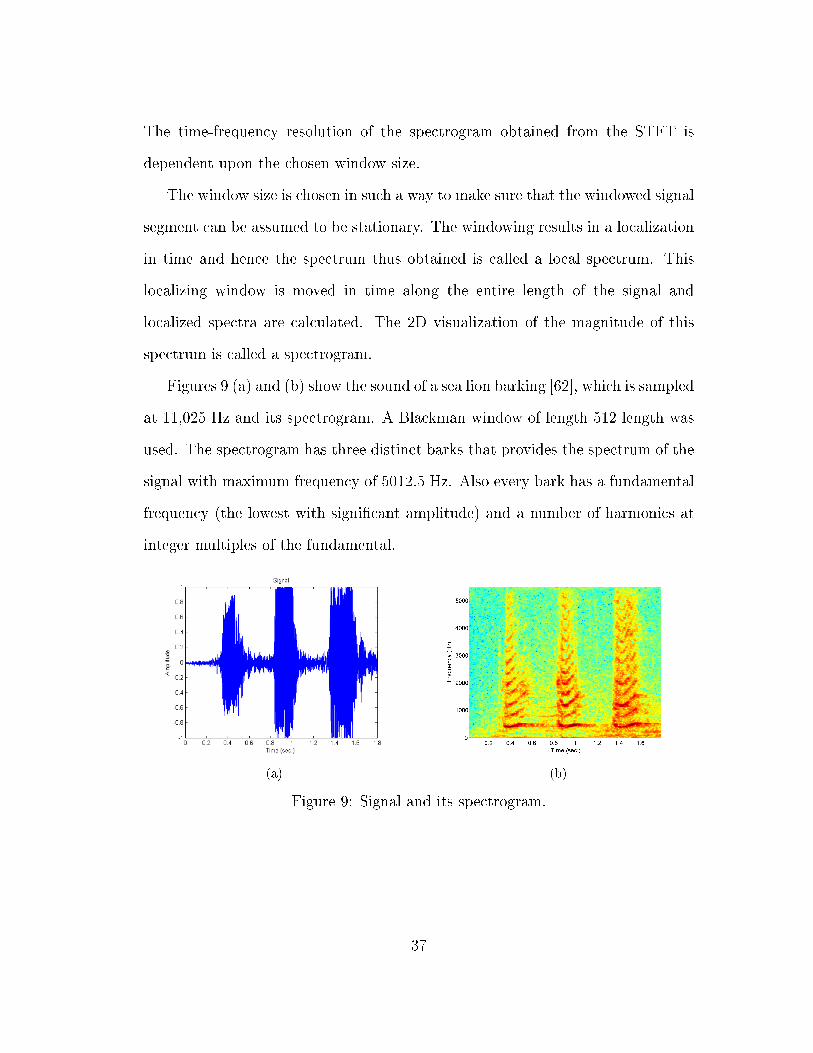
The time-frequency resolution of the spectrogram obtained from the STFT is

dependent upon the chosen window size.

The window size is chosen in such a way to make sure that the windowed signal

segment can be assumed to be stationary. The windowing results in a localization

in time and hence the spectrum thus obtained is called a local spectrum. This

localizing window is moved in time along the entire length of the signal and

localized spectra are calculated. The 2D visualization of the magnitude of this

spectrum is called a spectrogram.

Figures 9 (a) and (b) show the sound of a sea lion barking [62], which is sampled

at 11,025 Hz and its spectrogram. A Blackman window of length 512 length was

used. The spectrogram has three distinct barks that provides the spectrum of the

signal with maximum frequency of 5012.5 Hz. Also every bark has a fundamental

frequency (the lowest with signicant amplitude) and a number of harmonics at

integer multiples of the fundamental.

(a) (b)

Figure 9: Signal and its spectrogram.

37

5.3.1 Time Frequency Resolution Trade-o

Time resolution is dened as how well a transform can resolve rapid variations

in the time domain and frequency resolution refers to how well the changes in

frequencies of a signal can be tracked. The time and frequency resolution are

dependent directly on the width of the window used in time frequency analysis.

Frequency resolution is proportional to the bandwidth of the windowing function

while time resolution is proportional to the length of the windowing function.

Thus a short window is needed for good time resolution and a wider window

oers good frequency resolution.

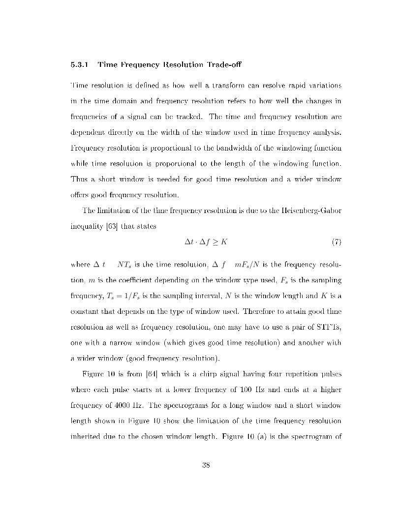
The limitation of the time frequency resolution is due to the Heisenberg-Gabor

inequality [63] that states

∆t ·∆f ≥ K (7)

where ∆ t = NTs is the time resolution, ∆ f =mFs/N is the frequency resolu-

tion, m is the coecient depending on the window type used, Fs is the sampling

frequency, Ts = 1/Fs is the sampling interval, N is the window length and K is a

constant that depends on the type of window used. Therefore to attain good time

resolution as well as frequency resolution, one may have to use a pair of STFTs,

one with a narrow window (which gives good time resolution) and another with

a wider window (good frequency resolution).

Figure 10 is from [64] which is a chirp signal having four repetition pulses

where each pulse starts at a lower frequency of 100 Hz and ends at a higher

frequency of 4000 Hz. The spectrograms for a long window and a short window

length shown in Figure 10 show the limitation of the time frequency resolution

inherited due to the chosen window length. Figure 10 (a) is the spectrogram of

38

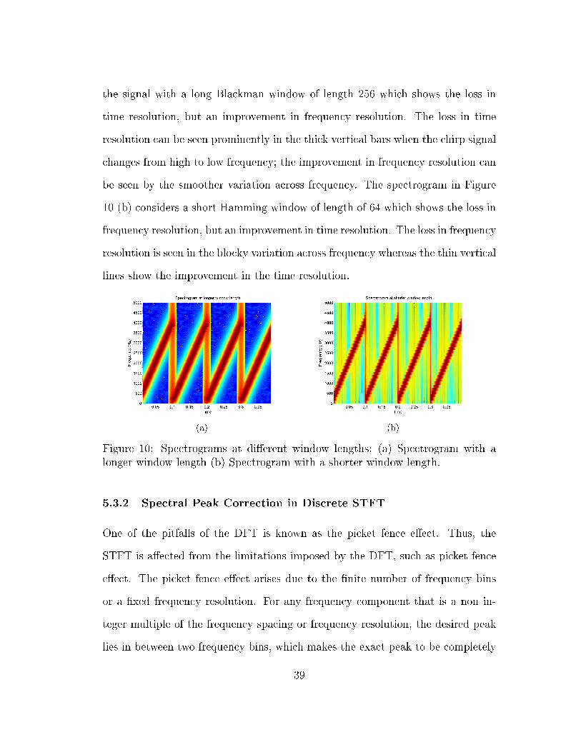
the signal with a long Blackman window of length 256 which shows the loss in

time resolution, but an improvement in frequency resolution. The loss in time

resolution can be seen prominently in the thick vertical bars when the chirp signal

changes from high to low frequency; the improvement in frequency resolution can

be seen by the smoother variation across frequency. The spectrogram in Figure

10 (b) considers a short Hamming window of length of 64 which shows the loss in

frequency resolution, but an improvement in time resolution. The loss in frequency

resolution is seen in the blocky variation across frequency whereas the thin vertical

lines show the improvement in the time resolution.

(a) (b)

Figure 10: Spectrograms at dierent window lengths; (a) Spectrogram with alonger window length (b) Spectrogram with a shorter window length.

5.3.2 Spectral Peak Correction in Discrete STFT

One of the pitfalls of the DFT is known as the picket fence eect. Thus, the

STFT is aected from the limitations imposed by the DFT, such as picket fence

eect. The picket fence eect arises due to the nite number of frequency bins

or a xed frequency resolution. For any frequency component that is a non in-

teger multiple of the frequency spacing or frequency resolution, the desired peak

lies in between two frequency bins, which makes the exact peak to be completely

39

indistinguishable. In addition, spectral leakage due to window sidelobes aect

the discrete STFT. Both xed frequency resolution and window eects result in

inaccurate measurement of harmonic and interharmonic components. To enhance

the resolution of the DFT and to identify the accurate peak of a frequency compo-

nent, a correction method based on three consecutive DFT samples was proposed

in [65]. Based on this approach, a frequency correction to the TFR obtained by

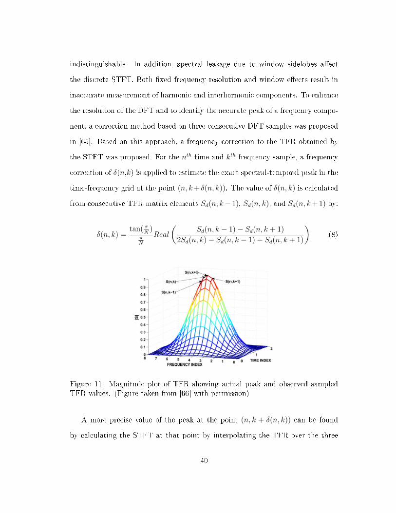
the STFT was proposed. For the nth time and kth frequency sample, a frequency

correction of δ(n,k) is applied to estimate the exact spectral-temporal peak in the

time-frequency grid at the point (n, k+ δ(n, k)). The value of δ(n, k) is calculated

from consecutive TFR matrix elements Sd(n, k− 1), Sd(n, k), and Sd(n, k+ 1) by:

δ(n, k) =tan( π

N)

πN

Real

(Sd(n, k − 1)− Sd(n, k + 1)

2Sd(n, k)− Sd(n, k − 1)− Sd(n, k + 1)

)(8)

Figure 11: Magnitude plot of TFR showing actual peak and observed sampledTFR values. (Figure taken from [66] with permission)

A more precise value of the peak at the point (n, k + δ(n, k)) can be found

by calculating the STFT at that point by interpolating the TFR over the three

40

consecutive TFR values Sd(n, k−1), Sd(n, k), and Sd(n, k+1) with a cubic spline

interpolation. Figure 11 illustrates the accurate peak detection.

5.3.3 Amplitude and Phase Correction in STFT

The time-frequency matrix S(n, k) can be computed with the STFT framework

for a window beginning at the nth time sample and for the kth frequency bin.

The estimation of amplitudes and phases for each row of the S matrix represent-

ing the harmonic and interharmonic frequency components requires correction in

amplitude as well as phase.

The frequency bin at k corresponding to the desired harmonic component in

the amplitude matrix of the complex S matrix is found for amplitude correction.

The amplitude correction for each element of the desired harmonic in the matrix

is multiplied by the corresponding amplication factor of the window used in the

STFT. The correction factor β is derived as

β(n, k) =

∣∣∣∣∣ 1− ej2πffsN

1− ej2π( ffs− kN

)

∣∣∣∣∣ (9)

where k represents the frequency bin of interest, fs is the sampling frequency, N

is the window length, and f is the frequency of the harmonic.

A signal waveform of the desired frequency component, whose phase is to

be estimated is used as a reference signal. The reference phases obtained from

the STFT matrix are used for phase correction. The reference phases are then

subtracted from the phases that are to be corrected. The phase dierence is

compared to a threshold (360 degrees or 2π radians), adjusted accordingly by

either subtracting or adding, and unwrapped.

41

6 METHODOLOGY

This chapter explains the methodology proposed in this thesis. The rst part

of this chapter describes a combination of an STFT framework and k- Nearest

Neighbor (k-NN) along with Support Vector Machine (SVM) classiers for the

identication and classication of dierent types of PQ disturbances in PQ mon-

itoring of particular interest here is a study of appropriate window lengths for an

STFT-based analysis of PQ events. The second part describes a real-time moni-

toring strategy based on the theoretical framework of the STFT focusing mainly

on the renewable rich electric power system, where the amplitudes and phases

of time varying harmonics and interharmonics, including the supraharmonics are

estimated. The second part then uses the same STFT based monitoring approach

in discriminating among dierent dynamic events. Two dynamic events, namely

fault and capacitor switching are considered for the discrimination.

6.1 Proposed Method for PQ Monitoring in Identication and Event

Classication Using STFT Framework

The proposed method for the PQ events identication and classication has three

key parts: pre-processing, feature extraction, and classication.

6.1.1 Pre-processing

In pre-processing of the proposed method, a normalization step is carried out. In

the normalization step, the event voltage waveform is converted to relative scale,

per unit (pu.) by dividing the input signal, by the nominal Root Mean Square

42

(RMS) voltage.

6.1.2 Feature Extraction

The time-frequency matrix S(n, k) can be computed with the STFT framework

for a window beginning at the nth time sample and for the kth frequency bin.

The column vector represents the signal's amplitude-frequency characteristic at a

particular moment whereas the row vector represents the time domain distribution

of signal in a certain frequency component.

By means of feature extraction, distinctive features of the disturbances are ob-

tained and the dimensionality of the feature space is lessened. Feature extraction

in this thesis is done by applying standard statistical techniques to each of the S

matrices obtained by applying the STFT to each PQ disturbance signal.

Features such as amplitude, slope (or gradient) of amplitude, time of occur-

rence, mean, standard deviation and energy of the transformed signal can be used

for the classication [33]. Features based on standard deviation (SD), energy,

mean amplitude, and mean frequency of the transformed signals are extracted.

6.1.3 Classication

For the purpose of classifying dierent PQ disturbances, a training database

formed by the extracted features is needed for PQ signals of dierent events or

classes. Features extracted from the signals are used as the input of a classication

system instead of the signal waveform itself. Selecting a proper set of features is

thus an important step toward successful classication. The classication accu-

racy depends upon the quality of the extracted features.

In this thesis, we employ two dierent classiers to determine the ecacy of

43

the extracted feature vector using the STFT framework in classifying dierent

PQ disturbance signals. We note that the study of the STFT for standard PQ

disturbances has been done before [11], [22], [31]. We include this analysis to com-

plement our study of the STFT specically for analysis of harmonics and inter-

harmonics including supraharmonics to demonstrate the versatility of the STFT

for PQ analysis. In particular, we demonstrate that STFT analysis with only a

few window lengths yield good results across a wide range of PQ disturbances,

including the dicult interharmonics and supraharmonics.

k-Nearest Neighbor Classier (k-NN) is a simple, linear classier. The

classier works by comparing a new sample (testing data) with the baseline data

(training data). The classier nds the k- neighborhood in the training data

and assigns the class which appear more frequently in the neighborhood of k.

Therefore, an object is classied by a majority vote of its neighbors, with the

object being assigned to the class most common amongst its k nearest neighbors,

where k is a typically small positive integer. The default value of k is 1. If k

= 1, then the object is simply assigned to the class of its nearest neighbor. In

a k-NN classier, dierent types of mathematical distances can be used to rate

all neighbors. Among them, k-NN classier with Euclidian distance is attractive

in the sense of reducing the processing time. The default distance setting is

Euclidean.

Support vector machine (SVM) belongs to the family of generalized linear

classiers [14]. A SVM separates two dierent groups of data by searching for

the hyperplane with maximum margin [39]. SVMs are able to nd non-linear

boundaries if classes are linearly non-separable. Each instance in the training set

contains one target value (class labels) and several attributes (features) [35].

44

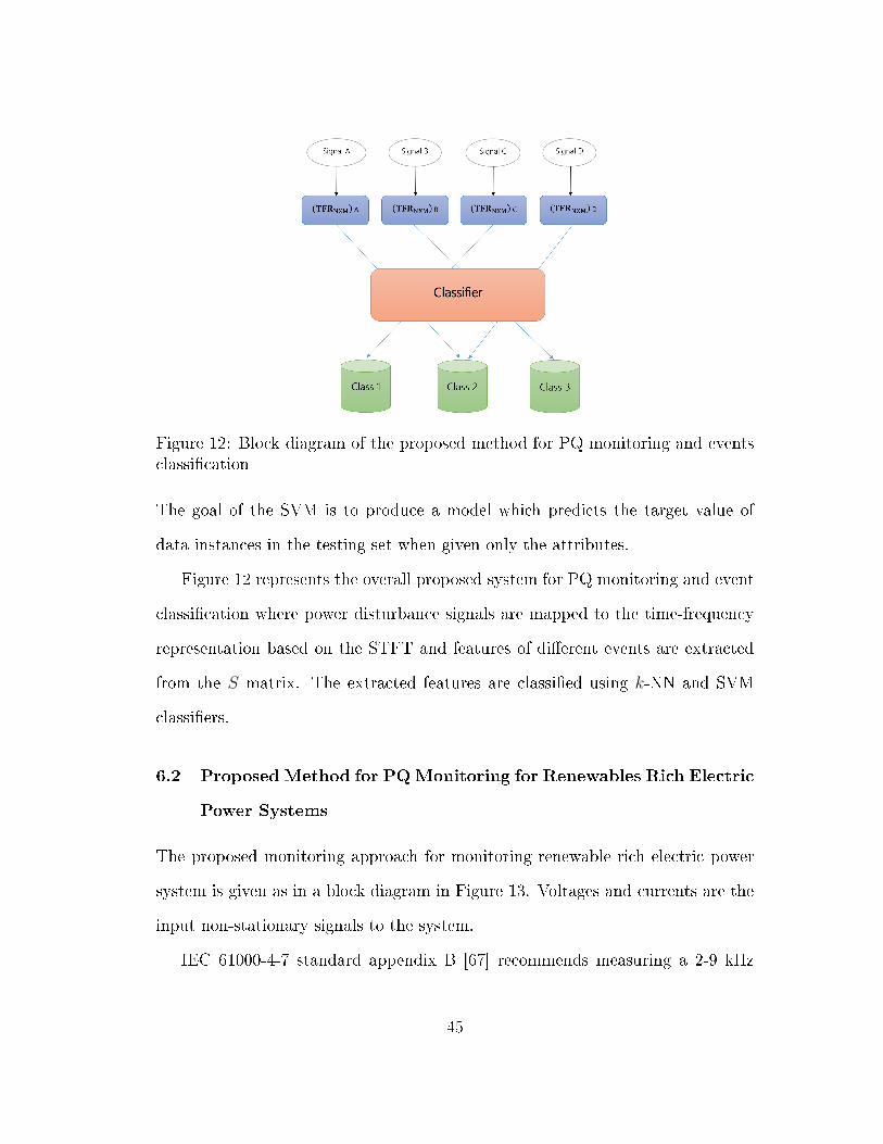
Figure 12: Block diagram of the proposed method for PQ monitoring and eventsclassication

The goal of the SVM is to produce a model which predicts the target value of

data instances in the testing set when given only the attributes.

Figure 12 represents the overall proposed system for PQ monitoring and event

classication where power disturbance signals are mapped to the time-frequency

representation based on the STFT and features of dierent events are extracted

from the S matrix. The extracted features are classied using k-NN and SVM

classiers.

6.2 Proposed Method for PQMonitoring for Renewables Rich Electric

Power Systems

The proposed monitoring approach for monitoring renewable rich electric power

system is given as in a block diagram in Figure 13. Voltages and currents are the

input non-stationary signals to the system.

IEC 61000-4-7 standard appendix B [67] recommends measuring a 2-9 kHz

45

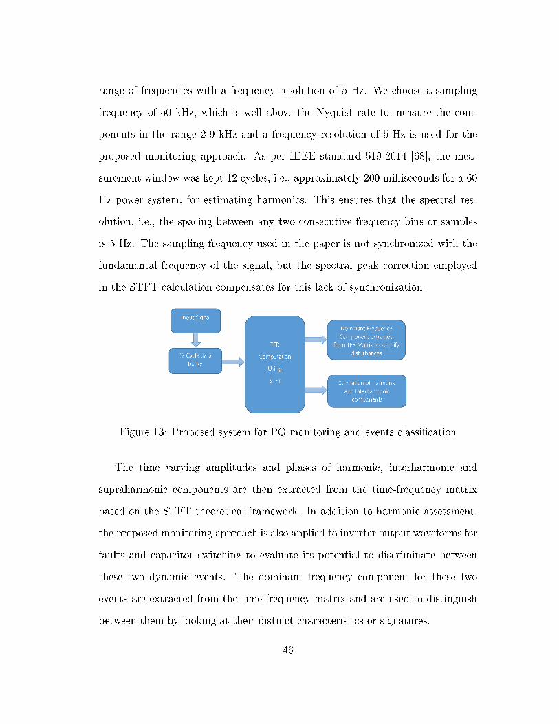
range of frequencies with a frequency resolution of 5 Hz. We choose a sampling

frequency of 50 kHz, which is well above the Nyquist rate to measure the com-

ponents in the range 2-9 kHz and a frequency resolution of 5 Hz is used for the

proposed monitoring approach. As per IEEE standard 519-2014 [68], the mea-

surement window was kept 12 cycles, i.e., approximately 200 milliseconds for a 60

Hz power system, for estimating harmonics. This ensures that the spectral res-

olution, i.e., the spacing between any two consecutive frequency bins or samples

is 5 Hz. The sampling frequency used in the paper is not synchronized with the

fundamental frequency of the signal, but the spectral peak correction employed

in the STFT calculation compensates for this lack of synchronization.

Figure 13: Proposed system for PQ monitoring and events classication

The time varying amplitudes and phases of harmonic, interharmonic and

supraharmonic components are then extracted from the time-frequency matrix

based on the STFT theoretical framework. In addition to harmonic assessment,

the proposed monitoring approach is also applied to inverter output waveforms for

faults and capacitor switching to evaluate its potential to discriminate between

these two dynamic events. The dominant frequency component for these two

events are extracted from the time-frequency matrix and are used to distinguish

between them by looking at their distinct characteristics or signatures.

46

7 EXPERIMENTAL RESULTS

This chapter details the experimental results obtained from the two proposed sys-

tems based on the theoretical framework of the STFT. The rst section documents

the result obtained during PQ monitoring in the identication and analysis based

on the STFT for dierent PQ disturbance signals. This section then evaluates the

performance of the two classiers used in classifying dierent PQ events, where

the overall accuracy obtained from each classier are documented. The second

section documents the estimated amplitude and phase results for time varying

harmonics. For interharmonics including supraharmonics, only estimated ampli-

tudes are presented. The second section concludes with the results obtained in

distinguishing between two dynamic events (fault and capacitor switching) using

the STFT based theoretical framework.

7.1 Data Generation for PQ Analysis

It is dicult to capture real-time PQ disturbance signals. Usually PQ disturbance

signals are produced by simulation for further analysis. Seven dierent PQ dis-

turbances have been generated using the mathematical models shown in Table 3,

at a sampling frequency of 50 kHz. Each PQ disturbance waveform consists of

12 cycles or approximately 200 ms for a 60 Hz power system (10000 data points).

The choice of a 50kHz sampling frequency is to be consistent with the analysis of

the harmonics, interharmonics and supraharmonics presented later.

47

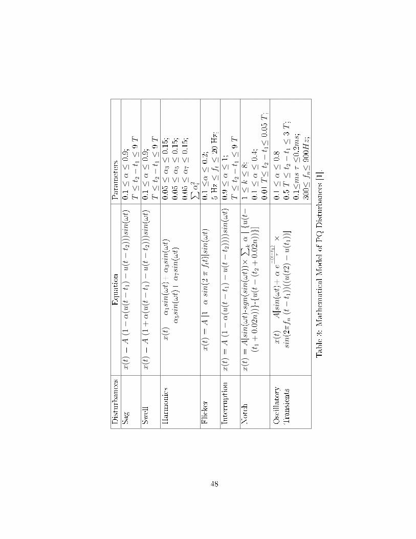
Disturbances

Equation

Param

eters

Sag

x(t

)=A

(1−α

(u(t−t 1

)−u

(t−t 2

)))sin(ωt)

0.1≤α≤

0.9;

T≤t 2−t 1≤

9T

Swell

x(t

)=A

(1+α

(u(t−t 1

)−u

(t−t 2

)))sin(ωt)

0.1≤α≤

0.9;

T≤t 2−t 1≤

9T

Harmonics

x(t

)=α

1sin(ωt)+α

3sin(ωt)

0.05≤α

3≤

0.15;

+α

5sin(ωt)+α

7sin(ωt)

0.05≤α

5≤

0.15;

0.05≤α

7≤

0.15;

∑ α2 iFlicker

x(t

)=A[1+αsin(2πf tt)]sin(ωt)

0.1≤α≤

0.2;

5Hz≤f t≤

20Hz;

Interruption

x(t

)=A

(1−α

(u(t−t 1

)−u

(t−t 2

))))sin(ωt)

0.9≤α≤

1;T≤t 2−t 1≤

9T

Notch

x(t

)=A[sin(ωt)-sgn(sin(ωt))×∑ k

α[u

(t−

1≤k≤

8;(t

1+

0.02n

))-u

(t−

(t2

+0.

02n

))]

0.1≤α≤

0.4;

0.01

T≤t 2−t 1≤

0.05

T;

Oscillatory

x(t

)=A[sin(ωt)+αe

−(t−t 1

)τ×

0.1≤α≤

0.8

Transients

sin(2πf n

(t−t 1

))((u

(t2)−u

(t1))]

0.5T≤t 2−t 1≤

3T;

0.1≤msτ≤0.2m

s;300≤

f n≤

900H

z;

Table3:

Mathem

aticalModelof

PQDisturbances[1].

48

7.2 PQ Analysis Using STFT

In this thesis, seven dierent types of PQ disturbances, namely voltage sag, swell,

interruption, icker, oscillatory transient, harmonic, and notch events are analyzed

and studied. The starting and ending time of PQ disturbances are varied but with

a predetermined range based on the parameters in Table 3. A Hamming window

length of 834 samples is used for computating the STFT matrix for the PQ analyis

for the disturbance signals in study.

For the nth time and kth frequency sample, the time-frequency matrix S(n, k)

can be computed with the STFT. The columns of the complex S matrix corre-

spond to the sampling time points whereas the rows correspond to the frequency

components (0 Hz to 25 kHz for a sampling frequency of 50 kHz). The rst

row (k=0) of the S matrix corresponds to the DC component and the frequency

dierence between adjacent rows is:

∆f = fs/N (10)

where N is the number of samples and fs is the sampling frequency.

The magnitude and phase of each element in the time-frequency matrix S

matrix can be calculated by:

ρS(n, k) =

√x(n, k)2 + y(n, k)2 (11)

θS((n, k)) = arctan(y(n, k)/x(n, k)) (12)

where S(n, k) =x(n, k) + jx(n, k) is the complex TF matrix, with j as the imagi-

nary unit. ρ(·) represents the calculation of magnitude and θ(·) is the calculation

49

of the phase. Each column of the matrix ρS can be ranked in order of size and the

frequency component with maximum amplitude is called the feature frequency

component, whose magnitude and phase are ρS,max and θS,max, respectively.

Figures 14-20 (a) show seven dierent types of PQ disturbance signals and the

time-frequency representation generated from the S matrix are shown in Figures

14-20 (b). The time-maximum amplitude plot of Figures 14-20 (c) represent the

maximum amplitude versus time obtained by searching columns of the S matrix

amplitude at every frequency. This denes the amplitude of the fundamental

frequency as it is has the largest amplitude. Figures 14-20 (d) represent the

frequency-maximum amplitude plot, presents maximum amplitudes versus nor-

malized frequency values, and the values in these plots are obtained by searching

the maximum value of the rows of the S matrix at every frequency.

In Figures 14-17 (d), there is only one peak at the fundamental frequency,

while in Figures 18-20 (d), there is more than one peak. This suggests that

the disturbances of voltage sag, swell, icker, and interruption have only the

fundamental frequency component, whereas the harmonics, oscillatory transient,

and notch have other frequency components.

The harmonic and oscillatory transient signals have more than one frequency

component, as shown in Figure 18 (d) and Figure 19 (d). Figures 18 (e) and

19 (e) are the frequency-mean amplitude plots which present mean amplitudes

versus normalized frequency values, and the values in these plots are obtained by

calculating the mean value of each row of the S matrix. The magnitude at the

high frequency in Figure 19 (e) is much lower than that in Figure 19 (d). This

illustrates that the transient disturbance is time varying whereas harmonic signal

is stable.

50

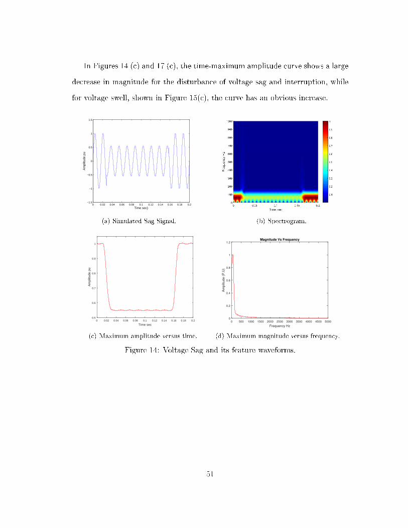
In Figures 14 (c) and 17 (c), the time-maximum amplitude curve shows a large

decrease in magnitude for the disturbance of voltage sag and interruption, while

for voltage swell, shown in Figure 15(c), the curve has an obvious increase.

0 0.02 0.04 0.06 0.08 0.1 0.12 0.14 0.16 0.18 0.2−1.5

−1

−0.5

0

0.5

1

1.5

Time sec)

Am

plitu

de p

u

(a) Simulated Sag Signal. (b) Spectrogram.

Time sec0 0.02 0.04 0.06 0.08 0.1 0.12 0.14 0.16 0.18 0.2

Am

plitu

de p

u

0.5

0.6

0.7

0.8

0.9

1

(c) Maximum amplitude versus time.

Frequency Hz

0 500 1000 1500 2000 2500 3000 3500 4000 4500 5000

Am

plit

ude (

P.U

)

0

0.2

0.4

0.6

0.8

1

1.2Magnitude Vs Frequency

(d) Maximum magnitude versus frequency.

Figure 14: Voltage Sag and its feature waveforms.

51

Time sec)0 0.02 0.04 0.06 0.08 0.1 0.12 0.14 0.16 0.18 0.2

Am

plitu

de p

u

-1.5

-1

-0.5

0

0.5

1

1.5

(a) Simulated Swell Signal. (b) Spectrogram.

Time sec0 0.02 0.04 0.06 0.08 0.1 0.12 0.14 0.16 0.18 0.2

Am

plitu

de p

u

0.95

1

1.05

1.1

1.15

1.2

1.25

1.3

(c) Maximum amplitude versus time.

Frequency Hz0 500 1000 1500 2000 2500 3000 3500 4000 4500 5000

Am

plitu

de p

u

0

0.2

0.4

0.6

0.8

1

1.2

1.4

(d) Maximum magnitude versus frequency.

Figure 15: Voltage Swell and its feature waveforms.

52

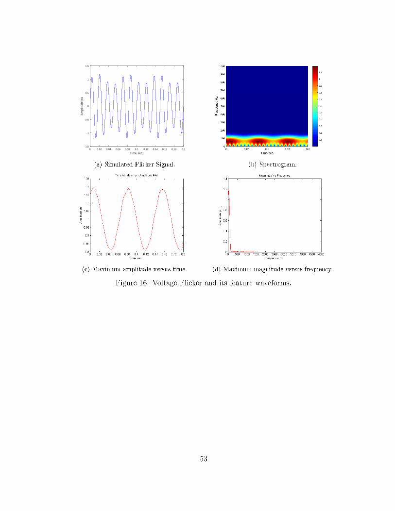
Time sec)0 0.02 0.04 0.06 0.08 0.1 0.12 0.14 0.16 0.18 0.2

Am

plitu

de p

u

-1.5

-1

-0.5

0

0.5

1

1.5

(a) Simulated Flicker Signal. (b) Spectrogram.

(c) Maximum amplitude versus time. (d) Maximum magnitude versus frequency.

Figure 16: Voltage Flicker and its feature waveforms.

53

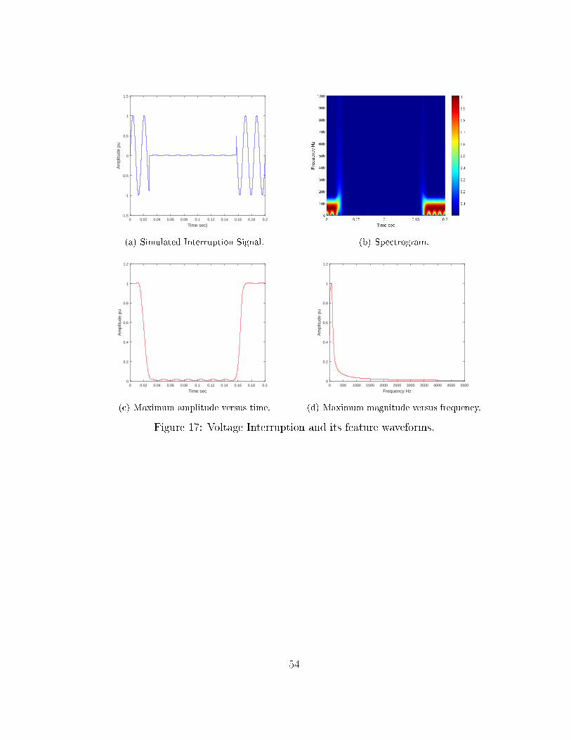
Time sec)0 0.02 0.04 0.06 0.08 0.1 0.12 0.14 0.16 0.18 0.2

Am

plitu

de p

u

-1.5

-1

-0.5

0

0.5

1

1.5

(a) Simulated Interruption Signal. (b) Spectrogram.

Time sec0 0.02 0.04 0.06 0.08 0.1 0.12 0.14 0.16 0.18 0.2

Am

plitu

de p

u

0

0.2

0.4

0.6

0.8

1

1.2

(c) Maximum amplitude versus time.

Frequency Hz0 500 1000 1500 2000 2500 3000 3500 4000 4500 5000

Am

plitu

de p

u

0

0.2

0.4

0.6

0.8

1

1.2

(d) Maximum magnitude versus frequency.

Figure 17: Voltage Interruption and its feature waveforms.

54

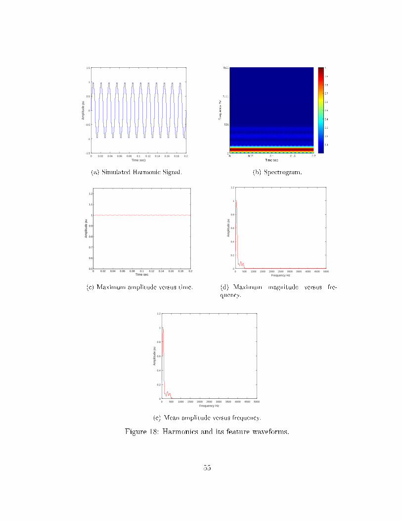
Time sec)0 0.02 0.04 0.06 0.08 0.1 0.12 0.14 0.16 0.18 0.2

Am

plitu

de p

u

-1.5

-1

-0.5

0

0.5

1

1.5

(a) Simulated Harmonic Signal. (b) Spectrogram.

0 0.02 0.04 0.06 0.08 0.1 0.12 0.14 0.16 0.18 0.20.5

0.6

0.7

0.8

0.9

1

1.1

1.2

Time sec

Am

plitu

de p

u

(c) Maximum amplitude versus time.

Frequency Hz0 500 1000 1500 2000 2500 3000 3500 4000 4500 5000

Am

plitu

de p

u

0

0.2

0.4

0.6

0.8

1

1.2

(d) Maximum magnitude versus fre-quency.

Frequency Hz0 500 1000 1500 2000 2500 3000 3500 4000 4500 5000

Am

plitu

de p

u

0

0.2

0.4

0.6

0.8

1

1.2

(e) Mean amplitude versus frequency.

Figure 18: Harmonics and its feature waveforms.

55

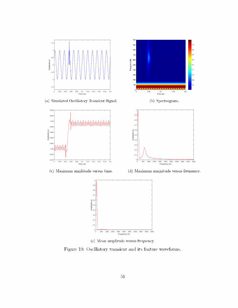
Time sec0 0.02 0.04 0.06 0.08 0.1 0.12 0.14 0.16 0.18 0.2

Am

plitu

de p

u

-1.5

-1

-0.5

0

0.5

1

1.5

(a) Simulated Oscillatory Transient Signal. (b) Spectrogram.

Time sec0 0.02 0.04 0.06 0.08 0.1 0.12 0.14 0.16 0.18 0.2

Am

plitu

de p

u

0.976

0.978

0.98

0.982

0.984

0.986

0.988

0.99

0.992

0.994

(c) Maximum amplitude versus time.

Frequency Hz0 500 1000 1500 2000 2500 3000 3500 4000 4500 5000

Am

plitu

de p

u

0

0.1

0.2

0.3

0.4

0.5

0.6

0.7

0.8

0.9

1

(d) Maximum magnitude versus frequency.

Frequency Hz0 500 1000 1500 2000 2500 3000 3500 4000 4500 5000

Am

plitu

de p

u

0

0.1

0.2

0.3

0.4

0.5

0.6

0.7

0.8

0.9

1

(e) Mean amplitude versus frequency.

Figure 19: Oscillatory transient and its feature waveforms.

56

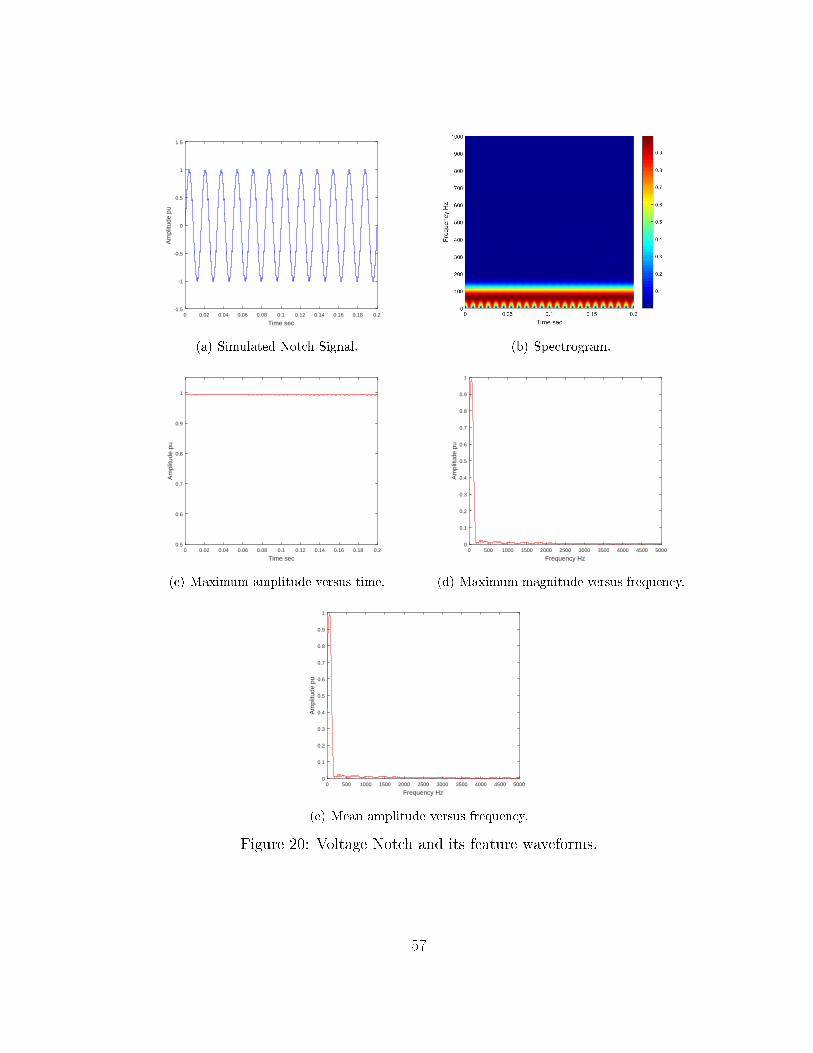
Time sec0 0.02 0.04 0.06 0.08 0.1 0.12 0.14 0.16 0.18 0.2

Am

plitu

de p

u

-1.5

-1

-0.5

0

0.5

1

1.5

(a) Simulated Notch Signal. (b) Spectrogram.

Time sec0 0.02 0.04 0.06 0.08 0.1 0.12 0.14 0.16 0.18 0.2

Am

plitu

de p

u

0.5

0.6

0.7

0.8

0.9

1

(c) Maximum amplitude versus time.

Frequency Hz0 500 1000 1500 2000 2500 3000 3500 4000 4500 5000

Am

plitu

de p

u

0

0.1

0.2

0.3

0.4

0.5

0.6

0.7

0.8

0.9

1

(d) Maximum magnitude versus frequency.

Frequency Hz0 500 1000 1500 2000 2500 3000 3500 4000 4500 5000

Am

plitu

de p

u

0

0.1

0.2

0.3

0.4

0.5

0.6

0.7

0.8

0.9

1

(e) Mean amplitude versus frequency.

Figure 20: Voltage Notch and its feature waveforms.

57

The dierence between voltage sag and interruption is the fall degree (slope of the

falling edge). The time-maximum amplitude plot of the interruption indicates a

bigger fall than that from a sag, shown in Figures 14 (c) and 17 (c), respectively.

The sag depth for voltage sag is 0.35 units with a sag duration of 0.1487

seconds as shown in Figure 21 (a). The interruption depth is 0.91125 units with

interruption duration of 0.1518 seconds as shown in Figure 21 (b). It can be

clearly seen that interruption has a larger fall and depth than a sag.

0 0.02 0.04 0.06 0.08 0.1 0.12 0.14 0.16 0.18 0.20.5

0.6

0.7

0.8

0.9

1

Time sec

Am

plitu

de p

u

Sag Duration= 0.1487 seconds

Sag Depth= 0.35 Units

(a)

0 0.02 0.04 0.06 0.08 0.1 0.12 0.14 0.16 0.18 0.20

0.2

0.4

0.6

0.8

1

1.2

1.4

Time sec

Am

plitu

de p

u

Interruption Duration = 0.1518 seconds

Interruption Depth = 0.91125 Units

(b)

Figure 21: (a) Sag depth and duration (b) Interruption depth and duration

58

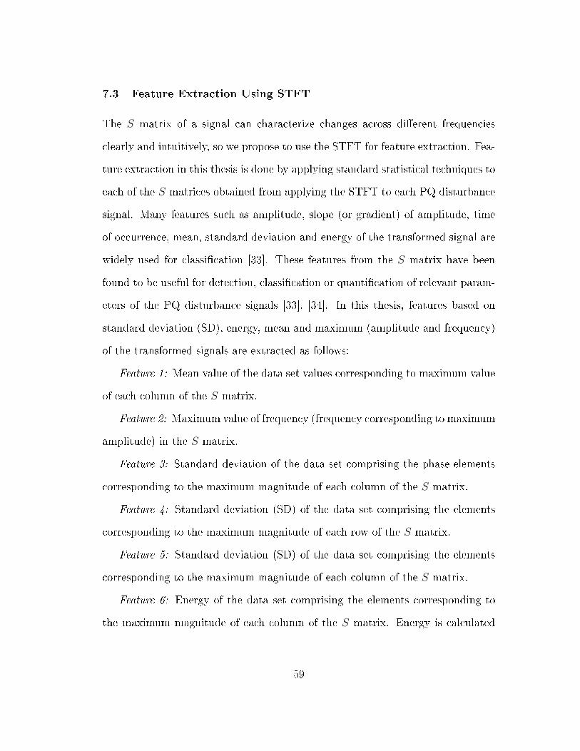
7.3 Feature Extraction Using STFT

The S matrix of a signal can characterize changes across dierent frequencies

clearly and intuitively, so we propose to use the STFT for feature extraction. Fea-

ture extraction in this thesis is done by applying standard statistical techniques to

each of the S matrices obtained from applying the STFT to each PQ disturbance

signal. Many features such as amplitude, slope (or gradient) of amplitude, time

of occurrence, mean, standard deviation and energy of the transformed signal are

widely used for classication [33]. These features from the S matrix have been

found to be useful for detection, classication or quantication of relevant param-

eters of the PQ disturbance signals [33], [34]. In this thesis, features based on

standard deviation (SD), energy, mean and maximum (amplitude and frequency)

of the transformed signals are extracted as follows:

Feature 1: Mean value of the data set values corresponding to maximum value

of each column of the S matrix.

Feature 2: Maximum value of frequency (frequency corresponding to maximum

amplitude) in the S matrix.

Feature 3: Standard deviation of the data set comprising the phase elements

corresponding to the maximum magnitude of each column of the S matrix.

Feature 4: Standard deviation (SD) of the data set comprising the elements

corresponding to the maximum magnitude of each row of the S matrix.

Feature 5: Standard deviation (SD) of the data set comprising the elements

corresponding to the maximum magnitude of each column of the S matrix.

Feature 6: Energy of the data set comprising the elements corresponding to

the maximum magnitude of each column of the S matrix. Energy is calculated

59

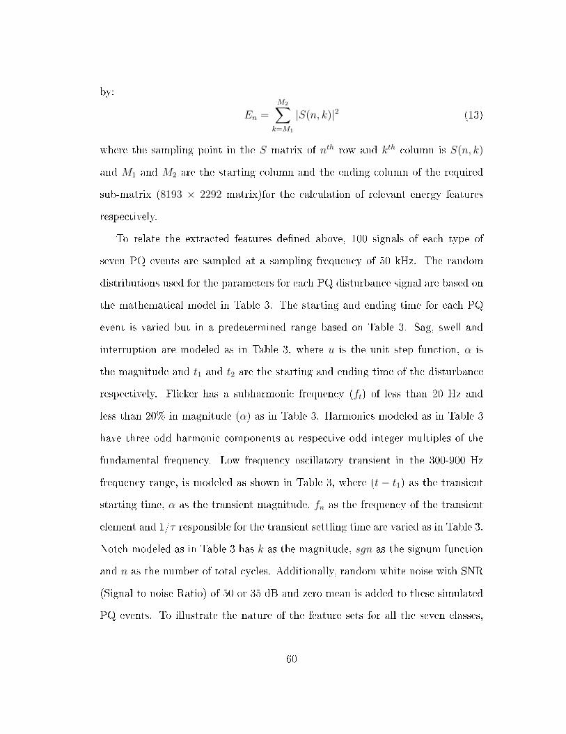
by:

En =

M2∑k=M1

|S(n, k)|2 (13)

where the sampling point in the S matrix of nth row and kth column is S(n, k)

and M1 and M2 are the starting column and the ending column of the required

sub-matrix (8193 × 2292 matrix)for the calculation of relevant energy features

respectively.

To relate the extracted features dened above, 100 signals of each type of

seven PQ events are sampled at a sampling frequency of 50 kHz. The random

distributions used for the parameters for each PQ disturbance signal are based on

the mathematical model in Table 3. The starting and ending time for each PQ

event is varied but in a predetermined range based on Table 3. Sag, swell and

interruption are modeled as in Table 3, where u is the unit step function, α is

the magnitude and t1 and t2 are the starting and ending time of the disturbance

respectively. Flicker has a subharmonic frequency (ft) of less than 20 Hz and

less than 20% in magnitude (α) as in Table 3. Harmonics modeled as in Table 3

have three odd harmonic components at respective odd integer multiples of the

fundamental frequency. Low frequency oscillatory transient in the 300-900 Hz

frequency range, is modeled as shown in Table 3, where (t − t1) as the transient

starting time, α as the transient magnitude, fn as the frequency of the transient

element and 1/τ responsible for the transient settling time are varied as in Table 3.

Notch modeled as in Table 3 has k as the magnitude, sgn as the signum function

and n as the number of total cycles. Additionally, random white noise with SNR

(Signal to noise Ratio) of 50 or 35 dB and zero mean is added to these simulated

PQ events. To illustrate the nature of the feature sets for all the seven classes,

60

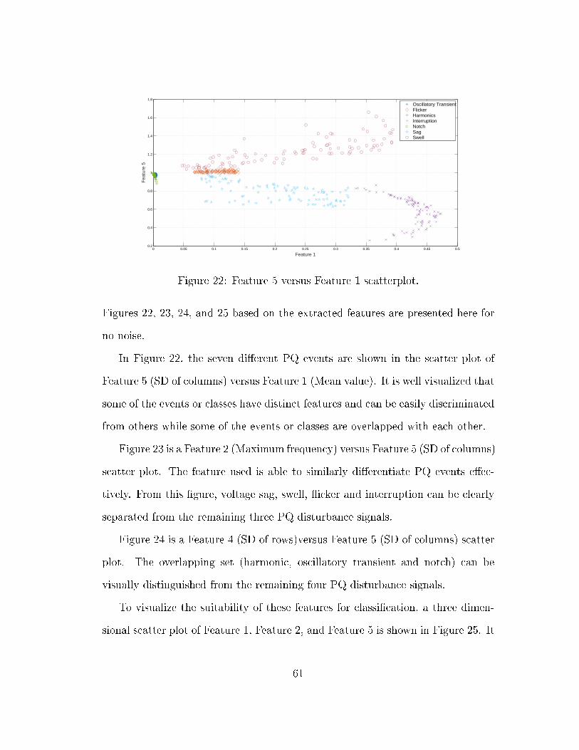
0 0.05 0.1 0.15 0.2 0.25 0.3 0.35 0.4 0.45 0.50.2

0.4

0.6

0.8

1

1.2

1.4

1.6

1.8

Feature 1

Fea

ture

5

Oscillatory TransientFlickerHarmonicsInterruptionNotchSagSwell

Figure 22: Feature 5 versus Feature 1 scatterplot.

Figures 22, 23, 24, and 25 based on the extracted features are presented here for

no noise.

In Figure 22, the seven dierent PQ events are shown in the scatter plot of

Feature 5 (SD of columns) versus Feature 1 (Mean value). It is well visualized that

some of the events or classes have distinct features and can be easily discriminated

from others while some of the events or classes are overlapped with each other.

Figure 23 is a Feature 2 (Maximum frequency) versus Feature 5 (SD of columns)

scatter plot. The feature used is able to similarly dierentiate PQ events eec-

tively. From this gure, voltage sag, swell, icker and interruption can be clearly

separated from the remaining three PQ disturbance signals.

Figure 24 is a Feature 4 (SD of rows)versus Feature 5 (SD of columns) scatter

plot. The overlapping set (harmonic, oscillatory transient and notch) can be

visually distinguished from the remaining four PQ disturbance signals.

To visualize the suitability of these features for classication, a three dimen-

sional scatter plot of Feature 1, Feature 2, and Feature 5 is shown in Figure 25. It

61

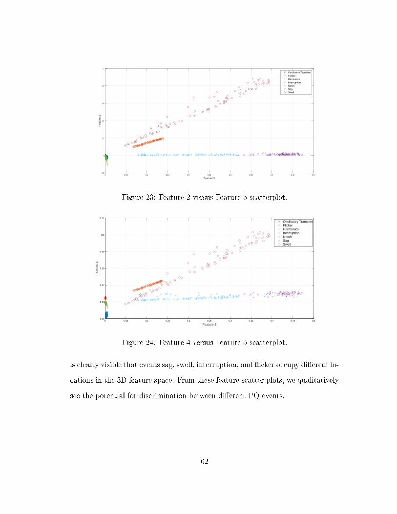
Feature 50 0.05 0.1 0.15 0.2 0.25 0.3 0.35 0.4 0.45 0.5

Fea

ture

2

0.8

1

1.2

1.4

1.6

1.8

2

Oscillatory TransientFlickerHarmonicsInterruptionNotchSagSwell

Figure 23: Feature 2 versus Feature 5 scatterplot.

0 0.05 0.1 0.15 0.2 0.25 0.3 0.35 0.4 0.45 0.50.05

0.06

0.07

0.08

0.09

0.1

0.11

Feature 5

Fea

ture

4

Oscillatory TransientFlickerHarmonicsInterruptionNotchSagSwell

Figure 24: Feature 4 versus Feature 5 scatterplot.

is clearly visible that events sag, swell, interruption, and icker occupy dierent lo-

cations in the 3D feature space. From these feature scatter plots, we qualitatively

see the potential for discrimination between dierent PQ events.

62

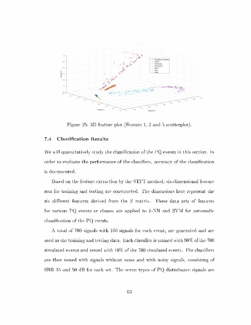
0.50.45

0.40.35

0.30.25

0.2

Feature 5

0.150.1

0.0500.2

0.4

0.6

Feature 1

0.8

1

1.2

1.4

1.6

0.8

1

1.2

1.4

1.6

1.8

2

1.8

Fea

ture

2Oscillatory TransientFlickerHarmonicsInterruptionNotchSagSwell

Figure 25: 3D feature plot (Feature 1, 2 and 5 scatterplot).

7.4 Classication Results

We will quantitatively study the classication of the PQ events in this section. In

order to evaluate the performance of the classiers, accuracy of the classication

is documented.

Based on the feature extraction by the STFT method, six-dimensional feature

sets for training and testing are constructed. The dimensions here represent the

six dierent features derived from the S matrix. These data sets of features

for various PQ events or classes are applied to k-NN and SVM for automatic

classication of the PQ events.

A total of 700 signals with 100 signals for each event, are generated and are

used as the training and testing data. Each classier is trained with 90% of the 700

simulated events and tested with 10% of the 700 simulated events. The classiers

are then tested with signals without noise and with noisy signals, consisting of

SNR 35 and 50 dB for each set. The seven types of PQ disturbance signals are

63

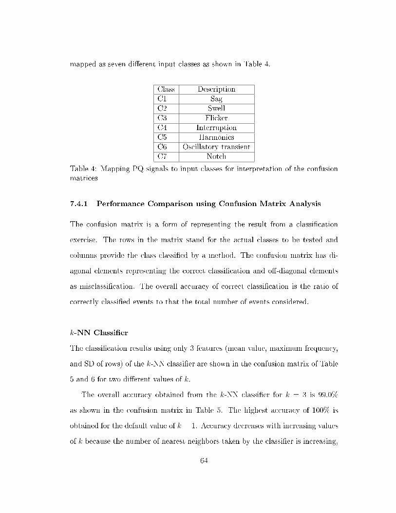
mapped as seven dierent input classes as shown in Table 4.

Class DescriptionC1 SagC2 SwellC3 FlickerC4 InterruptionC5 HarmonicsC6 Oscillatory transientC7 Notch

Table 4: Mapping PQ signals to input classes for interpretation of the confusionmatrices

7.4.1 Performance Comparison using Confusion Matrix Analysis

The confusion matrix is a form of representing the result from a classication

exercise. The rows in the matrix stand for the actual classes to be tested and

columns provide the class classied by a method. The confusion matrix has di-

agonal elements representing the correct classication and o-diagonal elements

as misclassication. The overall accuracy of correct classication is the ratio of

correctly classied events to that the total number of events considered.

k-NN Classier

The classication results using only 3 features (mean value, maximum frequency,

and SD of rows) of the k-NN classier are shown in the confusion matrix of Table

5 and 6 for two dierent values of k.

The overall accuracy obtained from the k-NN classier for k = 3 is 99.0%

as shown in the confusion matrix in Table 5. The highest accuracy of 100% is

obtained for the default value of k = 1. Accuracy decreases with increasing values

of k because the number of nearest neighbors taken by the classier is increasing,

64

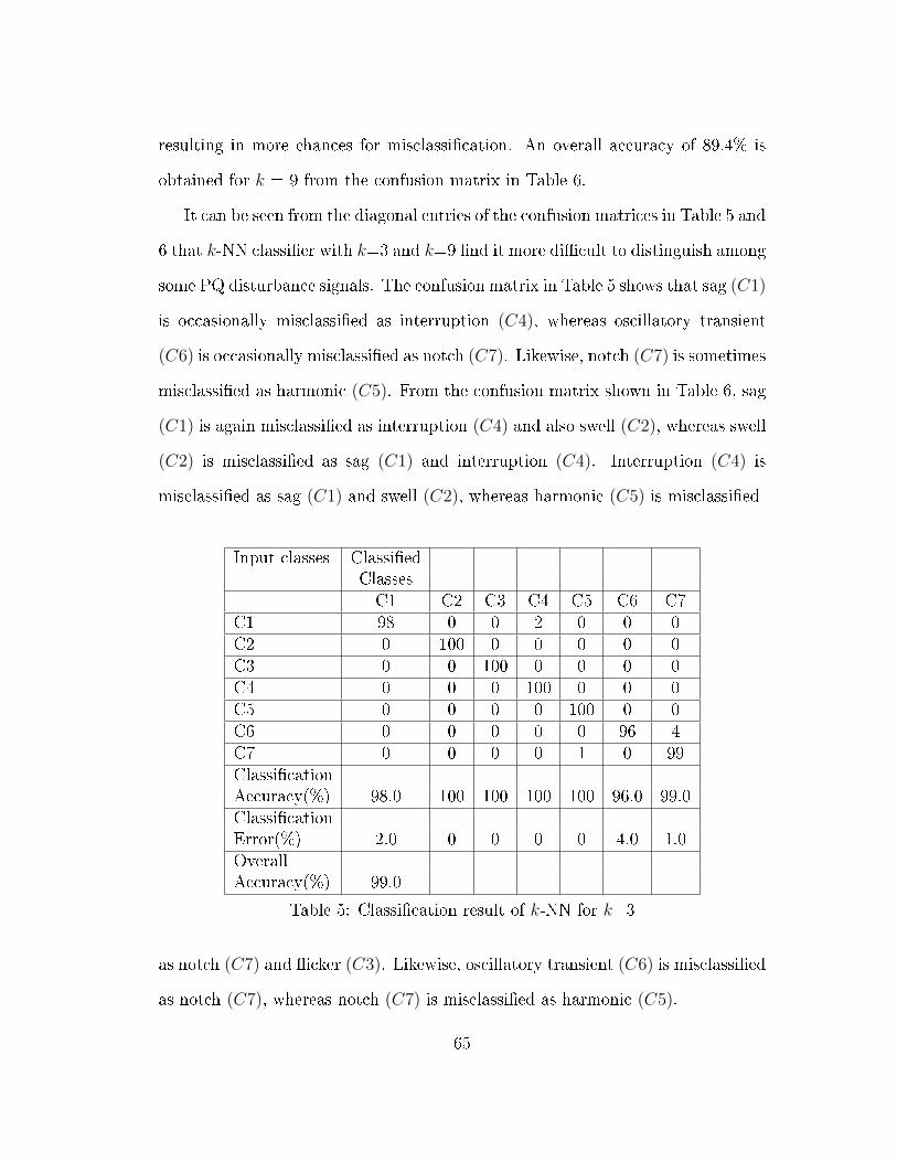
resulting in more chances for misclassication. An overall accuracy of 89.4% is

obtained for k = 9 from the confusion matrix in Table 6.

It can be seen from the diagonal entries of the confusion matrices in Table 5 and

6 that k-NN classier with k=3 and k=9 nd it more dicult to distinguish among

some PQ disturbance signals. The confusion matrix in Table 5 shows that sag (C1)

is occasionally misclassied as interruption (C4), whereas oscillatory transient

(C6) is occasionally misclassied as notch (C7). Likewise, notch (C7) is sometimes

misclassied as harmonic (C5). From the confusion matrix shown in Table 6, sag

(C1) is again misclassied as interruption (C4) and also swell (C2), whereas swell

(C2) is misclassied as sag (C1) and interruption (C4). Interruption (C4) is

misclassied as sag (C1) and swell (C2), whereas harmonic (C5) is misclassied

Input classes ClassiedClassesC1 C2 C3 C4 C5 C6 C7

C1 98 0 0 2 0 0 0C2 0 100 0 0 0 0 0C3 0 0 100 0 0 0 0C4 0 0 0 100 0 0 0C5 0 0 0 0 100 0 0C6 0 0 0 0 0 96 4C7 0 0 0 0 1 0 99ClassicationAccuracy(%) 98.0 100 100 100 100 96.0 99.0ClassicationError(%) 2.0 0 0 0 0 4.0 1.0OverallAccuracy(%) 99.0

Table 5: Classication result of k-NN for k=3

as notch (C7) and icker (C3). Likewise, oscillatory transient (C6) is misclassied

as notch (C7), whereas notch (C7) is misclassied as harmonic (C5).

65

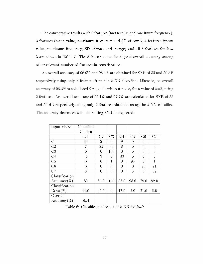
The comparative results with 2 features (mean value and maximum frequency),

3 features (mean value, maximum frequency and SD of rows), 4 features (mean

value, maximum frequency, SD of rows and energy) and all 6 features for k =

3 are shown in Table 7. The 3 features has the highest overall accuracy among

other relevant number of features in consideration.

An overall accuracy of 96.9% and 98.1% are obtained for SNR of 35 and 50 dB

respectively using only 3 features from the k-NN classier. Likewise, an overall

accuracy of 98.3% is calculated for signals without noise, for a value of k=3, using

2 features. An overall accuracy of 96.1% and 97.7% are calculated for SNR of 35

and 50 dB respectively using only 2 features obtained using the k-NN classier.

The accuracy decreases with decreasing SNR as expected.

Input classes ClassiedClassesC1 C2 C3 C4 C5 C6 C7

C1 89 2 0 9 0 0 0C2 7 85 0 8 0 0 0C3 0 0 100 0 0 0 0C4 15 2 0 83 0 0 0C5 0 0 1 0 98 0 1C6 0 0 0 0 0 79 21C7 0 0 0 0 8 0 92ClassicationAccuracy(%) 89 85.0 100 83.0 98.0 79.0 92.0ClassicationError(%) 11.0 15.0 0 17.0 2.0 21.0 8.0OverallAccuracy(%) 89.4

Table 6: Classication result of k-NN for k=9

66

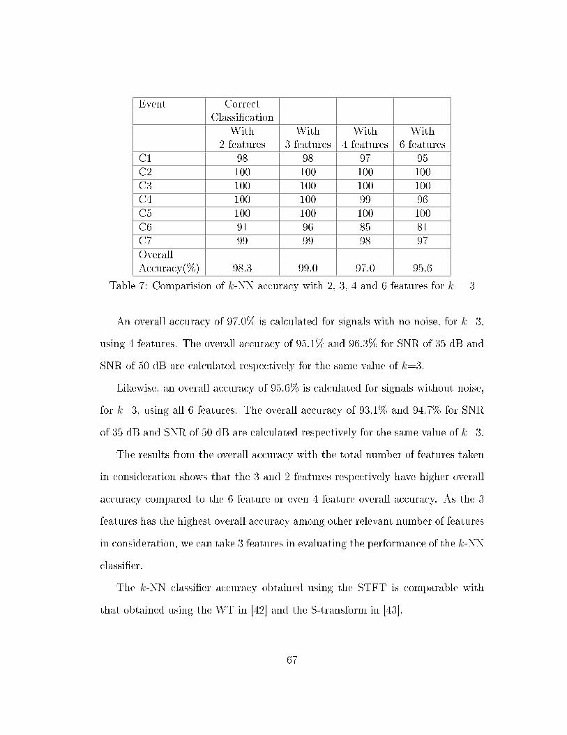
Event CorrectClassication

With With With With2 features 3 features 4 features 6 features

C1 98 98 97 95C2 100 100 100 100C3 100 100 100 100C4 100 100 99 96C5 100 100 100 100C6 91 96 85 81C7 99 99 98 97OverallAccuracy(%) 98.3 99.0 97.0 95.6

Table 7: Comparision of k-NN accuracy with 2, 3, 4 and 6 features for k = 3

An overall accuracy of 97.0% is calculated for signals with no noise, for k=3,

using 4 features. The overall accuracy of 95.1% and 96.3% for SNR of 35 dB and

SNR of 50 dB are calculated respectively for the same value of k=3.

Likewise, an overall accuracy of 95.6% is calculated for signals without noise,

for k=3, using all 6 features. The overall accuracy of 93.1% and 94.7% for SNR

of 35 dB and SNR of 50 dB are calculated respectively for the same value of k=3.

The results from the overall accuracy with the total number of features taken

in consideration shows that the 3 and 2 features respectively have higher overall

accuracy compared to the 6 feature or even 4 feature overall accuracy. As the 3

features has the highest overall accuracy among other relevant number of features

in consideration, we can take 3 features in evaluating the performance of the k-NN

classier.

The k-NN classier accuracy obtained using the STFT is comparable with

that obtained using the WT in [42] and the S-transform in [43].

67

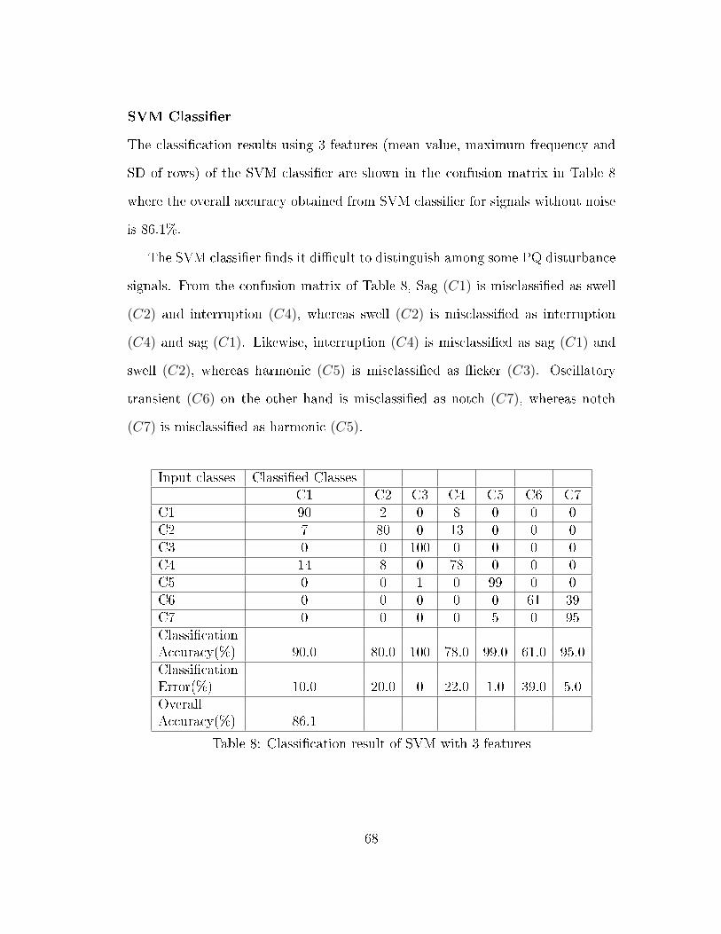
SVM Classier

The classication results using 3 features (mean value, maximum frequency and

SD of rows) of the SVM classier are shown in the confusion matrix in Table 8

where the overall accuracy obtained from SVM classier for signals without noise

is 86.1%.

The SVM classier nds it dicult to distinguish among some PQ disturbance

signals. From the confusion matrix of Table 8, Sag (C1) is misclassied as swell

(C2) and interruption (C4), whereas swell (C2) is misclassied as interruption

(C4) and sag (C1). Likewise, interruption (C4) is misclassied as sag (C1) and

swell (C2), whereas harmonic (C5) is misclassied as icker (C3). Oscillatory

transient (C6) on the other hand is misclassied as notch (C7), whereas notch

(C7) is misclassied as harmonic (C5).

Input classes Classied ClassesC1 C2 C3 C4 C5 C6 C7

C1 90 2 0 8 0 0 0C2 7 80 0 13 0 0 0C3 0 0 100 0 0 0 0C4 14 8 0 78 0 0 0C5 0 0 1 0 99 0 0C6 0 0 0 0 0 61 39C7 0 0 0 0 5 0 95ClassicationAccuracy(%) 90.0 80.0 100 78.0 99.0 61.0 95.0ClassicationError(%) 10.0 20.0 0 22.0 1.0 39.0 5.0OverallAccuracy(%) 86.1

Table 8: Classication result of SVM with 3 features

68

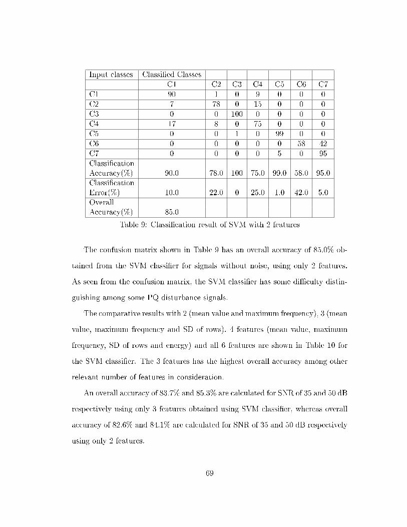
Input classes Classied ClassesC1 C2 C3 C4 C5 C6 C7

C1 90 1 0 9 0 0 0C2 7 78 0 15 0 0 0C3 0 0 100 0 0 0 0C4 17 8 0 75 0 0 0C5 0 0 1 0 99 0 0C6 0 0 0 0 0 58 42C7 0 0 0 0 5 0 95ClassicationAccuracy(%) 90.0 78.0 100 75.0 99.0 58.0 95.0ClassicationError(%) 10.0 22.0 0 25.0 1.0 42.0 5.0OverallAccuracy(%) 85.0

Table 9: Classication result of SVM with 2 features

The confusion matrix shown in Table 9 has an overall accuracy of 85.0% ob-

tained from the SVM classier for signals without noise, using only 2 features.

As seen from the confusion matrix, the SVM classier has some diculty distin-

guishing among some PQ disturbance signals.

The comparative results with 2 (mean value and maximum frequency), 3 (mean

value, maximum frequency and SD of rows), 4 features (mean value, maximum

frequency, SD of rows and energy) and all 6 features are shown in Table 10 for

the SVM classier. The 3 features has the highest overall accuracy among other

relevant number of features in consideration.

An overall accuracy of 83.7% and 85.3% are calculated for SNR of 35 and 50 dB

respectively using only 3 features obtained using SVM classier, whereas overall

accuracy of 82.6% and 84.1% are calculated for SNR of 35 and 50 dB respectively

using only 2 features.

69

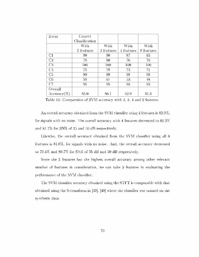
Event CorrectClassication

With With With With2 features 3 features 4 features 6 features

C1 90 90 87 85C2 78 80 76 76C3 100 100 100 100C4 75 78 73 71C5 99 99 98 98C6 58 61 53 48C7 95 95 93 93OverallAccuracy(%) 85.0 86.1 82.9 81.6

Table 10: Comparision of SVM accuracy with 2, 3, 4 and 6 features

An overall accuracy obtained from the SVM classier using 4 features is 82.9%,

for signals with no noise. The overall accuracy with 4 features decreased to 80.3%

and 81.7% for SNR of 35 and 50 dB respectively.

Likewise, the overall accuracy obtained from the SVM classier using all 6

features is 81.6%, for signals with no noise. And, the overall accuracy decreased

to 79.4% and 80.7% for SNR of 35 dB and 50 dB respectively.

Since the 3 features has the highest overall accuracy among other relevant

number of features in consideration, we can take 3 features in evaluating the

performance of the SVM classier.

The SVM classier accuracy obtained using the STFT is comparable with that

obtained using the S-transform in [39], [40] where the classier was trained on the

synthetic data.

70

7.5 Monitoring Harmonics and Interharmonics

We simulated the same test cases used in [66] with known parameters to evaluate

the performance of the proposed approach to measure time-varying harmonics,

including interharmonics and supraharmonics.

The test signal model is dened as:

x(n) =K∑k=1

Aksin(2πfkn

Fs+ φk) + ζ(n), (14)

where K denotes the maximum number of frequency components, fk is the fre-

quency of the kth spectral component, Ak and φk are, respectively, the instanta-

neous amplitude and phase of the kth spectral component, and ζ(n) is an additive

white Gaussian noise sequence with an SNR of 35 dB. A sampling frequency of

50 kHz is used in the simulation for the test signals in consideration in the study.

The selection of an appropriate window size is vital for the STFT [69]. How-

ever, the optimum window length will depend on the application. If the ap-

plication is such that we need time domain information to be more accurate, a

window of smaller size is preferred. If the application demands frequency domain

information to be more specic, a window of bigger size is preferred.

The best selection for the window length for our STFT computation is de-

termined by analyzing the respective Root Mean Square (RMS) estimation error

of amplitude and phase estimates for a range of window lengths. For estimation

71

accuracy, RMS estimation error was calculated according to

e(n) =

√√√√ 1

L

L∑n=1

(xd(n)− xe(n))2 (15)

where xd(n) and xe(n) are the desired and estimated signal components, respec-

tively, and L is the length of the dataset taken.

Figures 26 and 27 show the plots of RMS estimation error versus window length

for time-varying harmonics and inter-harmonics including supra-harmonics. The

smaller the RMS estimation error, the better the window length.

To determine the best window size possible, simulations are executed for both

harmonics and interharmonics including suprahramonics cases. For a signal with

time-varying harmonic components, the Hamming window size is varied between

400 samples and 1600 samples (8 ms - 32 ms, or 0.480 - 1.92 cycles of the fun-

damental). Figures have been zoomed to give a clear illustration showing the

calculated RMSE at the y-coordinate and window size at the x-coordinate in

both gures. A window size of 834 samples (16.68 ms, 1.0008 cycles) gives the

least RMS estimation error for harmonic components as shown in Figure 26 and

this window size is selected for estimating time-varying amplitude and phase of

signals with harmonics.

Likewise, for signals with inter-harmonics including supra-harmonic compo-

nents, the Hamming window size is varied between 700 samples and 1700 samples

(14 ms - 34 ms, or 0.84 - 2.04 cycles of the fundamental). For estimating the am-

plitude and phase of signals of time-varying inter-harmonics and supra harmonics,

a window size of 1600 samples (32 ms, 1.92 cycles of the fundamental) is selected

72

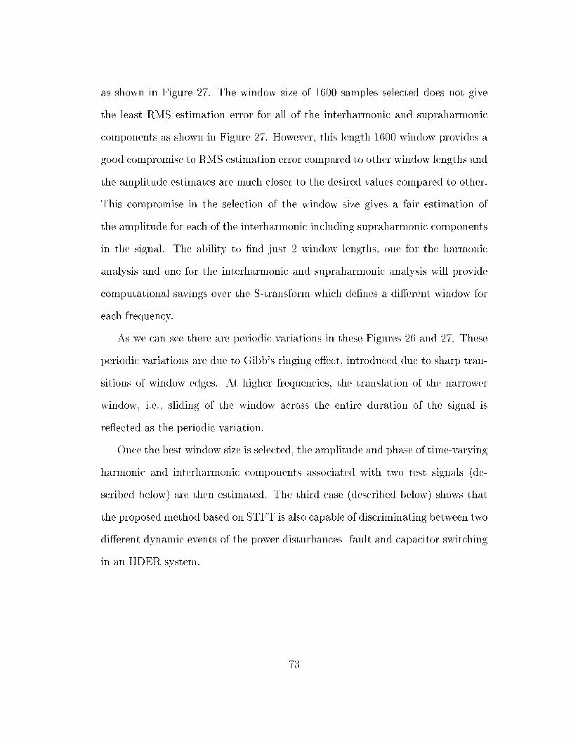
as shown in Figure 27. The window size of 1600 samples selected does not give

the least RMS estimation error for all of the interharmonic and supraharmonic

components as shown in Figure 27. However, this length 1600 window provides a

good compromise to RMS estimation error compared to other window lengths and

the amplitude estimates are much closer to the desired values compared to other.

This compromise in the selection of the window size gives a fair estimation of

the amplitude for each of the interharmonic including supraharmonic components

in the signal. The ability to nd just 2 window lengths, one for the harmonic

analysis and one for the interharmonic and supraharmonic analysis will provide

computational savings over the S-transform which denes a dierent window for

each frequency.

As we can see there are periodic variations in these Figures 26 and 27. These

periodic variations are due to Gibb's ringing eect, introduced due to sharp tran-

sitions of window edges. At higher frequencies, the translation of the narrower

window, i.e., sliding of the window across the entire duration of the signal is

reected as the periodic variation.

Once the best window size is selected, the amplitude and phase of time-varying

harmonic and interharmonic components associated with two test signals (de-

scribed below) are then estimated. The third case (described below) shows that

the proposed method based on STFT is also capable of discriminating between two

dierent dynamic events of the power disturbances- fault and capacitor switching

in an IIDER system.

73

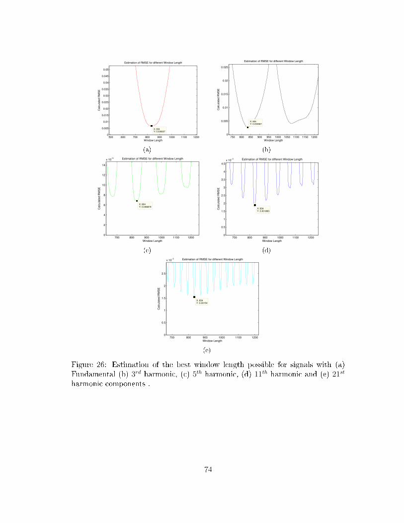
500 600 700 800 900 1000 1100 12000

0.005

0.01

0.015

0.02

0.025

0.03

0.035

0.04

0.045

0.05

X: 834Y: 0.006837

Window Length

Ca

lcu

late

d R

MS

E

Estimation of RMSE for different Window Length

(a)

750 800 850 900 950 1000 1050 1100 1150 12000

0.005

0.01

0.015

0.02

0.025

X: 834Y: 0.002667

Window Length

Ca

lcu

late

d R

MS

E

Estimation of RMSE for different Window Length

(b)

700 800 900 1000 1100 12000

2

4

6

8

10

12

14

x 10−3

X: 834Y: 0.006819

Window Length

Ca

lcu

late

d R

MS

E

Estimation of RMSE for different Window Length

(c)

700 800 900 1000 1100 12000

0.5

1

1.5

2

2.5

3

3.5

4

4.5

x 10−3

X: 834Y: 0.001883

Window Length

Ca

lcu

late

d R

MS

E

Estimation of RMSE for different Window Length

(d)

700 800 900 1000 1100 12000

0.5

1

1.5

2

2.5

x 10−3

X: 834Y: 0.00154

Window Length

Ca

lcu

late

d R

MS

E

Estimation of RMSE for different Window Length

(e)

Figure 26: Estimation of the best window length possible for signals with (a)Fundamental (b) 3rd harmonic, (c) 5th harmonic, (d) 11th harmonic and (e) 21st

harmonic components .

74

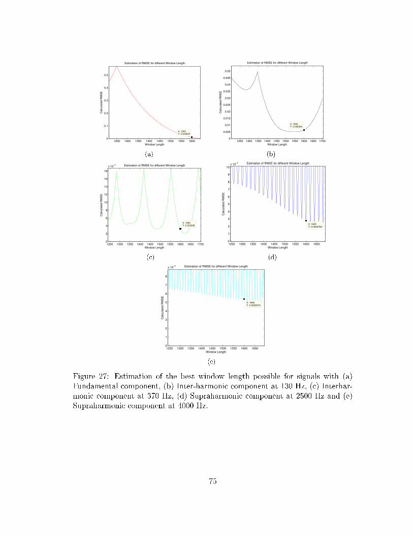
1250 1300 1350 1400 1450 1500 1550 16000

0.1

0.2

0.3

0.4

0.5

X: 1600Y: 0.009923

Window Length

Calc

ula

ted R

MS

E

Estimation of RMSE for different Window Length

(a)

1250 1300 1350 1400 1450 1500 1550 1600 1650 17000

0.005

0.01

0.015

0.02

0.025

0.03

0.035

0.04

0.045

0.05

X: 1600Y: 0.006304

Window Length

Ca

lcu

late

d R

MS

E

Estimation of RMSE for different Window Length

(b)

1250 1300 1350 1400 1450 1500 1550 1600 1650 17000

2

4

6

8

10

12

14

16

18

x 10−3

X: 1600Y: 0.003208

Window Length

Calc

ula

ted R

MS

E

Estimation of RMSE for different Window Length

(c)

1250 1300 1350 1400 1450 1500 1550 1600 16500

1

2

3

4

5

6

7

8

9

10x 10

−4

X: 1600Y: 0.0002762

Window Length

Ca

lcu

late

d R

MS

E

Estimation of RMSE for different Window Length

(d)

1250 1300 1350 1400 1450 1500 1550 1600 16500

1

2

3

4

5

6

7

8

x 10−4

X: 1600Y: 0.0005374

Window Length

Ca

lcu

late

d R

MS

E

Estimation of RMSE for different Window Length

(e)

Figure 27: Estimation of the best window length possible for signals with (a)Fundamental component, (b) Inter-harmonic component at 130 Hz, (c) Interhar-monic component at 370 Hz, (d) Supraharmonic component at 2500 Hz and (e)Supraharmonic component at 4000 Hz.

75

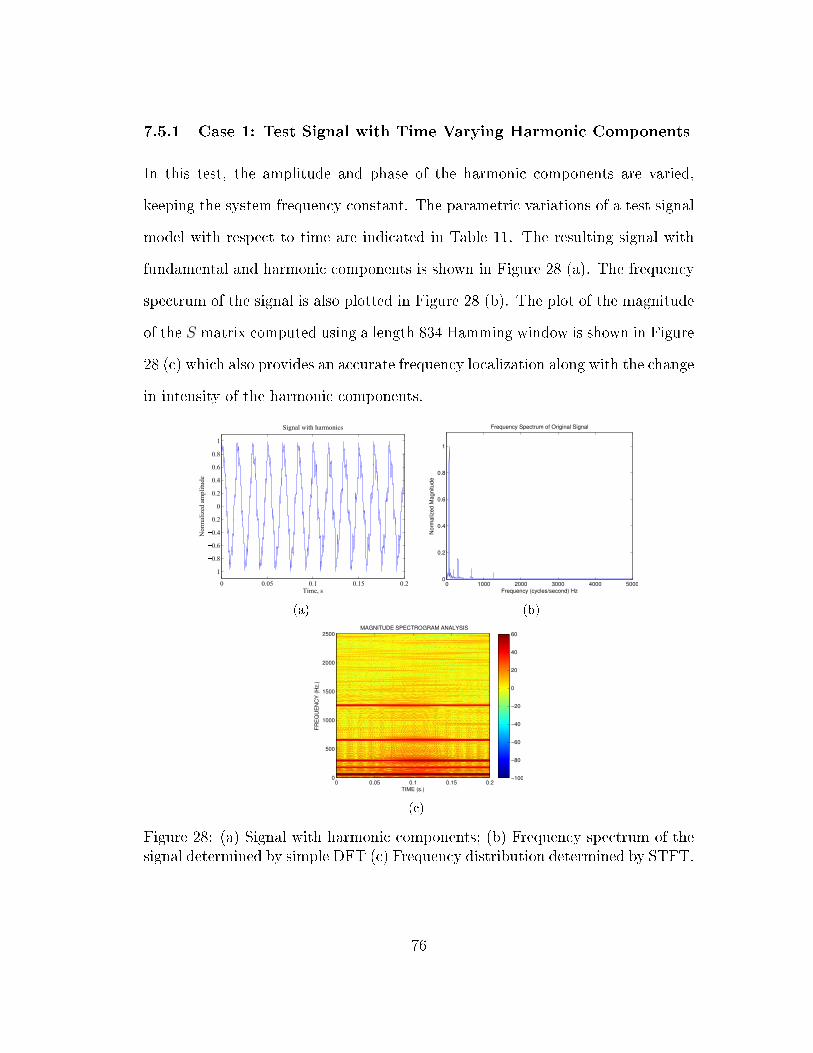
7.5.1 Case 1: Test Signal with Time Varying Harmonic Components

In this test, the amplitude and phase of the harmonic components are varied,

keeping the system frequency constant. The parametric variations of a test signal

model with respect to time are indicated in Table 11. The resulting signal with

fundamental and harmonic components is shown in Figure 28 (a). The frequency

spectrum of the signal is also plotted in Figure 28 (b). The plot of the magnitude

of the S matrix computed using a length 834 Hamming window is shown in Figure

28 (c) which also provides an accurate frequency localization along with the change

in intensity of the harmonic components.

0 0.05 0.1 0.15 0.2

1

0.8

0.6

0.4

0.2

0

0.2

0.4

0.6

0.8

1

Time, s

Norm

aliz

ed a

mpli

tude

Signal with harmonics

(a)

0 1000 2000 3000 4000 50000

0.2

0.4

0.6

0.8

1

Frequency (cycles/second) Hz

Norm

aliz

ed M

agnitude

Frequency Spectrum of Original Signal

(b)

TIME (s.)

FR

EQ

UE

NC

Y (

Hz.)

MAGNITUDE SPECTROGRAM ANALYSIS

0 0.05 0.1 0.15 0.2

0

500

1000

1500

2000

2500

−100

−80

−60

−40

−20

0

20

40

60

(c)

Figure 28: (a) Signal with harmonic components; (b) Frequency spectrum of thesignal determined by simple DFT (c) Frequency distribution determined by STFT.

76

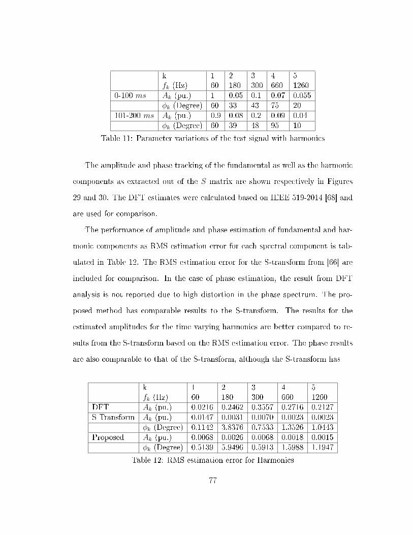
k 1 2 3 4 5fk (Hz) 60 180 300 660 1260

0-100 ms Ak (pu.) 1 0.05 0.1 0.07 0.055φk (Degree) 60 33 43 75 20

101-200 ms Ak (pu.) 0.9 0.08 0.2 0.09 0.04φk (Degree) 60 39 48 95 10

Table 11: Parameter variations of the test signal with harmonics

The amplitude and phase tracking of the fundamental as well as the harmonic

components as extracted out of the S matrix are shown respectively in Figures

29 and 30. The DFT estimates were calculated based on IEEE 519-2014 [68] and

are used for comparison.

The performance of amplitude and phase estimation of fundamental and har-

monic components as RMS estimation error for each spectral component is tab-

ulated in Table 12. The RMS estimation error for the S-transform from [66] are

included for comparison. In the case of phase estimation, the result from DFT

analysis is not reported due to high distortion in the phase spectrum. The pro-

posed method has comparable results to the S-transform. The results for the

estimated amplitudes for the time varying harmonics are better compared to re-

sults from the S-transform based on the RMS estimation error. The phase results

are also comparable to that of the S-transform, although the S-transform has

k 1 2 3 4 5fk (Hz) 60 180 300 660 1260

DFT Ak (pu.) 0.0216 0.2462 0.3557 0.2716 0.2127S Transform Ak (pu.) 0.0147 0.0031 0.0070 0.0023 0.0023

φk (Degree) 0.1142 3.8376 0.7533 1.3526 1.0443Proposed Ak (pu.) 0.0068 0.0026 0.0068 0.0018 0.0015

φk (Degree) 0.5139 5.9496 0.5913 1.5988 1.1947

Table 12: RMS estimation error for Harmonics

77

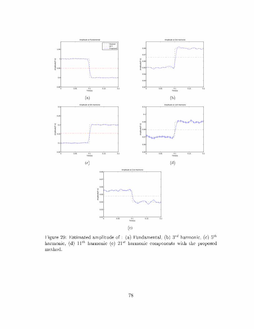
0 0.05 0.1 0.15 0.20.85

0.9

0.95

1

1.05

Time(s)

Am

plitu

de(P

.U)

Amplitude at Fundamental

DesiredDFTProposed

(a)

0 0.05 0.1 0.15 0.20.02

0.03

0.04

0.05

0.06

0.07

0.08

Time(s)

Am

plitu

de(P

.U)

Amplitude at 3rd Harmonic

(b)

0 0.05 0.1 0.15 0.20.05

0.1

0.15

0.2

0.25

0.3

Time(s)

Am

plitu

de(P

.U)

Amplitude at 5th Harmonic

(c)

0 0.05 0.1 0.15 0.20.05

0.06

0.07

0.08

0.09

0.1

0.11

Time(s)

Am

plitu

de(P

.U)

Amplitude at 11th Harmonic

(d)

0 0.05 0.1 0.15 0.20.02

0.03

0.04

0.05

0.06

0.07

0.08

Time(s)

Am

plitu

de(P

.U)

Amplitude at 21st Harmonic

(e)

Figure 29: Estimated amplitude of : (a) Fundamental, (b) 3rd harmonic, (c) 5th

harmonic, (d) 11th harmonic (e) 21st harmonic components with the proposedmethod.

78

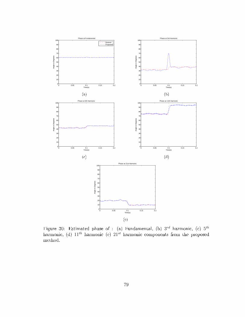
0 0.05 0.1 0.15 0.20

10

20

30

40

50

60

70

80

90

100

Time(s)

Ang

le in

Deg

rees

Phase at Fundamental

DesiredProposed

(a)

0 0.05 0.1 0.15 0.20

10

20

30

40

50

60

70

80

90

100

Time(s)

Ang

le in

Deg

rees

Phase at 3rd Harmonic

(b)

0 0.05 0.1 0.15 0.20

10

20

30

40

50

60

70

80

90

100

Time(s)

Ang

le in

Deg

rees

Phase at 5th Harmonic

(c)

0 0.05 0.1 0.15 0.20

10

20

30

40

50

60

70

80

90

100

Time(s)

Ang

le in

Deg

rees

Phase at 11th Harmonic

(d)

0 0.05 0.1 0.15 0.20

10

20

30

40

50

60

70

80

90

100

Time(s)

Ang

le in

Deg

rees

Phase at 21st Harmonic

(e)

Figure 30: Estimated phase of : (a) Fundamental, (b) 3rd harmonic, (c) 5th

harmonic, (d) 11th harmonic (e) 21st harmonic components from the proposedmethod.

79

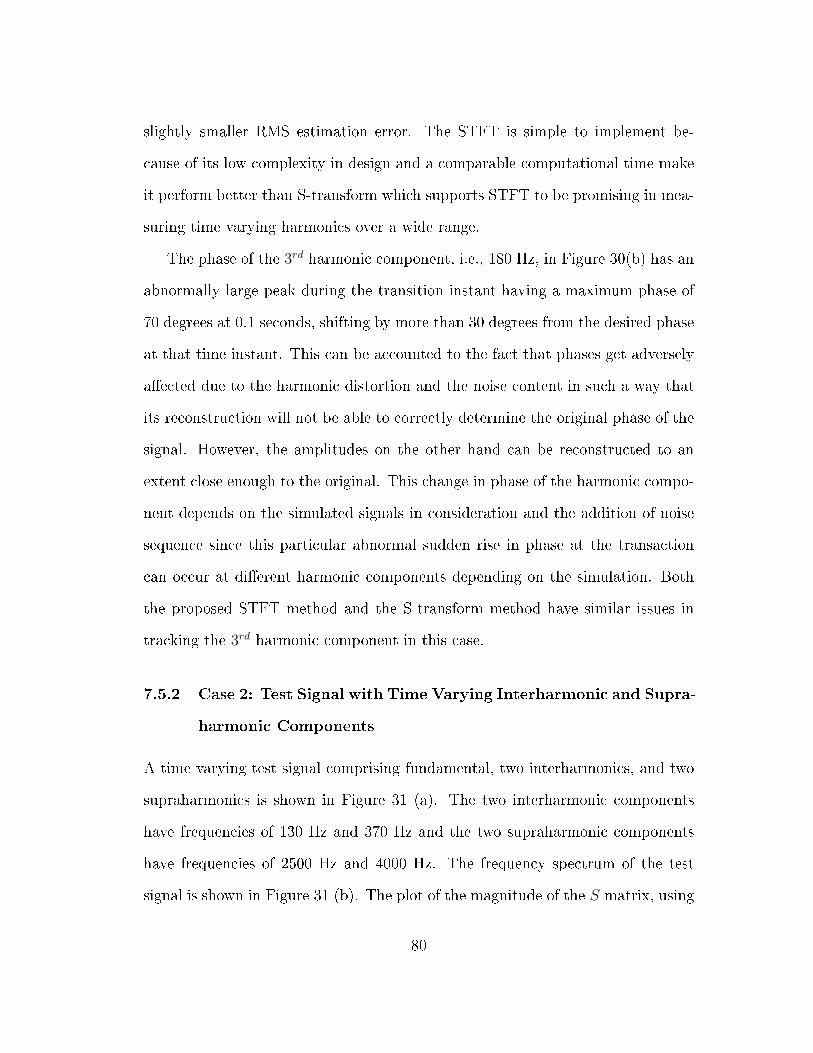
slightly smaller RMS estimation error. The STFT is simple to implement be-

cause of its low complexity in design and a comparable computational time make

it perform better than S-transform which supports STFT to be promising in mea-

suring time varying harmonics over a wide range.

The phase of the 3rd harmonic component, i.e., 180 Hz, in Figure 30(b) has an

abnormally large peak during the transition instant having a maximum phase of

70 degrees at 0.1 seconds, shifting by more than 30 degrees from the desired phase

at that time instant. This can be accounted to the fact that phases get adversely

aected due to the harmonic distortion and the noise content in such a way that

its reconstruction will not be able to correctly determine the original phase of the

signal. However, the amplitudes on the other hand can be reconstructed to an

extent close enough to the original. This change in phase of the harmonic compo-

nent depends on the simulated signals in consideration and the addition of noise

sequence since this particular abnormal sudden rise in phase at the transaction

can occur at dierent harmonic components depending on the simulation. Both

the proposed STFT method and the S-transform method have similar issues in

tracking the 3rd harmonic component in this case.

7.5.2 Case 2: Test Signal with Time Varying Interharmonic and Supra-

harmonic Components

A time varying test signal comprising fundamental, two interharmonics, and two

supraharmonics is shown in Figure 31 (a). The two interharmonic components

have frequencies of 130 Hz and 370 Hz and the two supraharmonic components

have frequencies of 2500 Hz and 4000 Hz. The frequency spectrum of the test

signal is shown in Figure 31 (b). The plot of the magnitude of the S matrix, using

80

a length-1600 Hamming window is shown in Figure 31 (c) which also provides an

accurate frequency localization by observing the plot. The change in intensity of

the interharmonic components can also be observed from the gure. The ampli-

tude variations of these spectral components with respect to time are shown in

Table 13.

k 1 2 3 4 5fk (Hz) 60 130 370 2500 4000

0-100 ms Ak (pu.) 1 0.06 0.02 0.012 0.010101-200 ms Ak (pu.) 1 0.09 0.04 0.01 0.015

Table 13: Parameter variations of the test signal with Interharmonic and Supra-harmonic components

0 0.05 0.1 0.15 0.2

1

0.8

0.6

0.4

0.2

0

0.2

0.4

0.6

0.8

1

Time, s

No

rmal

ized

am

pli

tud

e

Signal with interharmonics and supraharmonics

(a)

0 1000 2000 3000 4000 50000

0.2

0.4

0.6

0.8

1

Frequency (cycles/second) Hz

No

rma

lize

d M

ag

nitu

de

Frequency Spectrum of Signal

(b)

TIME (s.)

FR

EQ

UE

NC

Y (

Hz.)

MAGNITUDE SPECTROGRAM ANALYSIS

0 0.05 0.1 0.15 0.2

0

500

1000

1500

2000

2500

3000

3500

4000

4500

5000

−100

−80

−60

−40

−20

0

20

40

60

(c)

Figure 31: (a) Signal with interharmonic components (b) Frequency spectrum ofthe signal determined by simple DFT, and (c) Frequency distribution determinedby STFT.

81

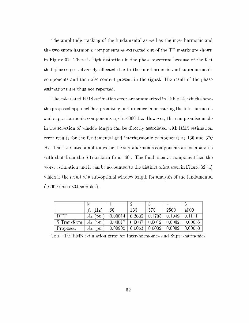
The amplitude tracking of the fundamental as well as the inter-harmonic and

the two supra harmonic components as extracted out of the TF matrix are shown

in Figure 32. There is high distortion in the phase spectrum because of the fact

that phases get adversely aected due to the interharmonic and supraharmonic

components and the noise content present in the signal. The result of the phase

estimations are thus not reported.

The calculated RMS estimation error are summarized in Table 14, which shows

the proposed approach has promising performance in measuring the interharmonic

and supra-harmonic components up to 4000 Hz. However, the compromise made

in the selection of window length can be directly associated with RMS estimation

error results for the fundamental and interharmonic components at 130 and 370

Hz. The estimated amplitudes for the supraharmonic components are comparable

with that from the S-transform from [66]. The fundamental component has the

worst estimation and it can be accounted to the distinct oset seen in Figure 32 (a)

which is the result of a sub-optimal window length for analysis of the fundamental

(1600 versus 834 samples).

k 1 2 3 4 5fk (Hz) 60 130 370 2500 4000

DFT Ak (pu.) 0.00014 0.2632 0.1705 0.1049 0.1111S Transform Ak (pu.) 0.00017 0.0037 0.0012 0.0002 0.00035Proposed Ak (pu.) 0.00992 0.0063 0.0032 0.0002 0.00053

Table 14: RMS estimation error for Inter-harmonics and Supra-harmonics

82

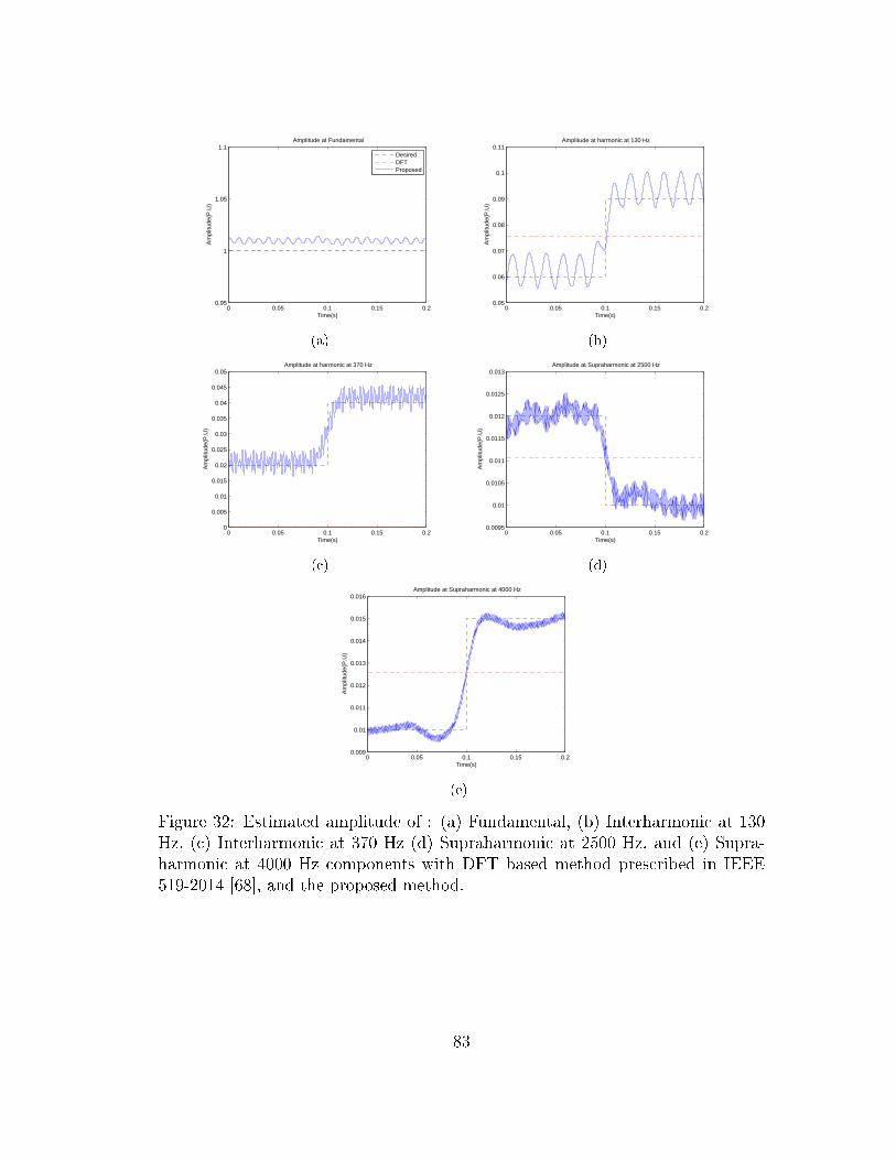
0 0.05 0.1 0.15 0.20.95

1

1.05

1.1

Time(s)

Am

plitu

de(P

.U)

Amplitude at Fundamental

DesiredDFTProposed

(a)

0 0.05 0.1 0.15 0.20.05

0.06

0.07

0.08

0.09

0.1

0.11

Time(s)

Am

plitu

de(P

.U)

Amplitude at harmonic at 130 Hz

(b)

0 0.05 0.1 0.15 0.20

0.005

0.01

0.015

0.02

0.025

0.03

0.035

0.04

0.045

0.05

Time(s)

Am

plitu

de(P

.U)

Amplitude at harmonic at 370 Hz

(c)

0 0.05 0.1 0.15 0.20.0095

0.01

0.0105

0.011

0.0115

0.012

0.0125

0.013

Time(s)

Am

plitu

de(P

.U)

Amplitude at Supraharmonic at 2500 Hz

(d)

0 0.05 0.1 0.15 0.20.009

0.01

0.011

0.012

0.013

0.014

0.015

0.016

Time(s)

Am

plitu

de(P

.U)

Amplitude at Supraharmonic at 4000 Hz

(e)

Figure 32: Estimated amplitude of : (a) Fundamental, (b) Interharmonic at 130Hz, (c) Interharmonic at 370 Hz (d) Supraharmonic at 2500 Hz, and (e) Supra-harmonic at 4000 Hz components with DFT based method prescribed in IEEE519-2014 [68], and the proposed method.

83

7.5.3 Case 3: Discriminating Disturbances in an IIDER System

The test signals comprising two dynamic events are the output current reading of

the inverter and are from [66]. The current signals are analyzed and the calculated

S matrix, using a length-834 Hamming window from the proposed method is

shown in Figure 33. The visually distinct dominant frequency component during

the disturbances - fault and capacitor switching, in a disturbed state are shown

in Figure 33. Both of these dynamic events show distinct visual characteristics or

signatures that dier from each other, using the same window length as for the

harmonic analysis.

These two dynamic events- fault and capacitor switching are analyzed simply

by observing the inverter currents. The previous comprehensive classication case

study were on voltage signals only.

The extracted dominant frequency component, which is the time-maximum

amplitude, during the disturbances is achieved by seeking columns of the STFT

matrix amplitude at every frequency. The fault as observed has a continual pos-

itive deviation with reference to the base value, whereas capacitor switching has

several oscillations per cycle. The results show that detection and distinction

between these disturbances is possible and can be done within a one-cycle time,

using the same window length as for the harmonic analysis.

84

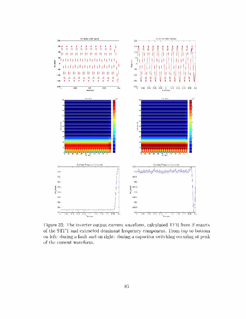
Figure 33: The inverter output current waveform, calculated TFR from S matrixof the STFT and extracted dominant frequency component. From top to bottomon left: during a fault and on right: during a capacitor switching occuring at peakof the current waveform.

85

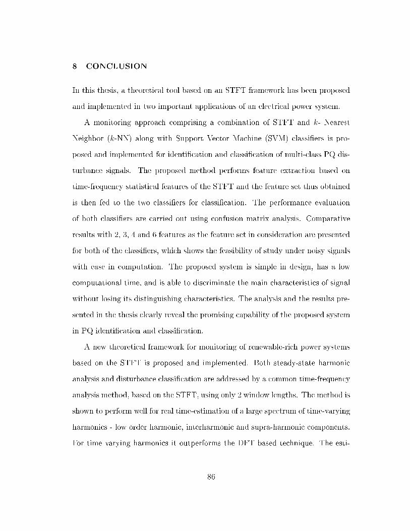
8 CONCLUSION

In this thesis, a theoretical tool based on an STFT framework has been proposed

and implemented in two important applications of an electrical power system.

A monitoring approach comprising a combination of STFT and k- Nearest

Neighbor (k-NN) along with Support Vector Machine (SVM) classiers is pro-

posed and implemented for identication and classication of multi-class PQ dis-

turbance signals. The proposed method performs feature extraction based on

time-frequency statistical features of the STFT and the feature set thus obtained

is then fed to the two classiers for classication. The performance evaluation

of both classiers are carried out using confusion matrix analysis. Comparative

results with 2, 3, 4 and 6 features as the feature set in consideration are presented

for both of the classiers, which shows the feasibility of study under noisy signals

with ease in computation. The proposed system is simple in design, has a low

computational time, and is able to discriminate the main characteristics of signal

without losing its distinguishing characteristics. The analysis and the results pre-

sented in the thesis clearly reveal the promising capability of the proposed system

in PQ identication and classication.

A new theoretical framework for monitoring of renewable-rich power systems

based on the STFT is proposed and implemented. Both steady-state harmonic

analysis and disturbance classication are addressed by a common time-frequency

analysis method, based on the STFT, using only 2 window lengths. The method is

shown to perform well for real time-estimation of a large spectrum of time-varying

harmonics - low order harmonic, interharmonic and supra-harmonic components.

For time varying harmonics it outperforms the DFT based technique. The esti-

86

mated amplitudes for the time varying harmonics from the proposed method are

found better compared to the S-transform results. The estimated phases are also

comparable. Also, the proposed approach has promising performance in measur-

ing supraharmonic components up to 4000 Hz. Verication over representative

simulated waveforms show the potential capability of the proposed method in

uniquely identifying two dynamic events for which inverter currents appear simi-

lar - faults and capacitor switchings, in less than a cycle, by simply analyzing the

inverter currents.

87

9 FUTURE WORK

The future work will be focused on extensively analyzing the capability of

the proposed TFA tool for a comprehensive PQ monitoring solution with online

classication capabilities for an electrical power system.

The eectiveness of the classication method can be improved through clus-

tering analysis using the inter-class separability and intra-class compactness, and

increasing the training and testing data set used in the classication.

The distinct peak at 180 Hz of the phase estimate for harmonics from the

proposed method and S-transform can be studied. Also, a median ltering can be

implemented for the estimation of amplitude and phase for better performance.

Implementing a sliding-window estimation of signal parameters via rotational

invariance techniques (ESPRIT) in PQ monitoring may solve the long existing

problem of quantifying interharmonic components when there is no preknowledge

of their frequencies [70].

Particular attention will be on the assessment with eld data, automated dis-

turbance detection and diagnosis, and computational issues.

88

REFERENCES

[1] IEEE Recommended Practice for Monitoring Electric Power Quality, IEEEStd. 1159-2009.

[2] J. Arrillaga, M. H. J. Bollen and N. R. Waston , 2000a. Power quality fol-lowing deregulation, Proc. IEEE., vol. 88, no. 2, pp. 246-261.

[3] J. Arrillaga, N. R. Watson, and S. Chen, 2000b. Power System Quality As-sessment, John Wiley and Sons Ltd., London.

[4] R. C. Dugan, M. F. McGranaghan, S. Santoso, and H. W. Beaty, ElectricalPower System Quality, 2nd Edn., McGraw Hill Book Company, New York,2003.

[5] IEEE Recommended Practice for Industrial and Commercial Power SystemsAnalysis, IEEE Std. 399-1997.

[6] J. J. Burke , D. C. Grith , and J. Ward , Power quality - Two dierentperspectives,, IEEE Trans. on Power Delivery, vol. 5, pp. 1501 1513, 1990.

[7] F. Mark, McGranagham, and S. Santoso, Challenges and trends in analysisof electric power quality measurement data, EURASIP. J. Adv. Signal Proc.,1: 171 - 177, 2007.

[8] M. H. J. Bollen. Understanding Power Quality Problems: Voltage Sags andInterruptions. Wiley-IEEE Press, 2000.

[9] J. Stones and A. Collinson, Power Quality, IEEE Power Engineering Jour-nal, pp. 58-64, April 2001.

[10] Electromagnetic Compatibility, Limits - Assessment of Emission Limits forDistorting Loads in MV and HV Power Systems", Technical Report IEC-61000, Ed. I, International Electro-Technical Commission, 1996.

[11] Y. H. Gu and M. H. Bollen, Time-frequency and time-scale domain analysisof voltage disturbances," IEEE Trans. on Power Delivery, vol. 15, no. 4, pp.1279 - 1284, 2000.

[12] W. M. Lin, C. H. Wu, C. H. Lin, and F. S. Cheng, Detection and classica-tion of multiple power-quality disturbances with wavelet multi-class SVM,"IEEE Transactions on Power Delivery, vol. 23, no. 4, pp. 2575 - 2582, 2008.

89

[13] M. Chilukuri and P. Dash, Multiresolution S-transform-based fuzzy recogni-tion system for power quality events," IEEE Transactions on Power Delivery,vol. 19, no. 1, pp. 323 - 330, 2004.

[14] C. Chunling, X. Tongyu, P. Zailin, and Y. Ye, Power quality disturbancesclassication based on multi-class classication SVM," in Power Electronicsand Intelligent Transportation System (PEITS), 2nd International Confer-ence. IEEE, vol. 1. , pp. 290 - 294, 2009.

[15] M. H. Bollen, L. Yao, S. K. Ronnberg, and M. Wahlberg, Harmonic andinterharmonic distortion due to a windpark, IEEE Power and Energy SocietyGeneral Meeting. IEEE, vol. 3, pp. 1 6, 2010.

[16] S. Papathanassiou and M. P. Papadopoulos, Harmonic analysis in a powersystem with wind generation, IEEE Transactions on Power Delivery, vol. 21,no. 4, pp. 4-7, 2006.

[17] S. T. Tentzerakis, and S. Papathanassiou, An investigation of the harmonicemissions of wind turbines, IEEE Transactions on Energy Conversion, vol.22, no. 1, pp. 150 158, 2007.

[18] E. W. Gunther and H. Mehta, A survey of distribution system power qualitypreliminary results, IEEE Transactions on Power Delivery, vol. 10, no. 1, pp.322 - 329, Jan. 1995.

[19] M. B. Hughes, J. S. Chan, and D. O. Koval, Distribution customer powerquality experience, IEEE Transactions on Industrial. Applications, vol. 29,no. 1, pp. 1204 - 1211, Nov./Dec. 1993.

[20] IEEE Recommended Practice for Monitoring Electric Power Quality, IEEEInc., New York, USA, 1995.

[21] R. A. Flores, State of the art in the classication of power quality events: anoverview," IEEE, 10th International Conference on Harmonics and Qualityof Power, vol. 1., pp. 17 - 20, 2002.

[22] A. Gaouda, S. Kanoun, and M. Salama, On-line disturbance classicationusing nearest neighbor rule, Electric Power Systems Research, vol. 57, no.1, pp. 1 - 8, 2001.

[23] T. Y. Vega, V. F. Riog, and H. B. S Segundo, Evolution of Signal ProcessingTechniques in Power Quality, 9th International Conference Electrical Power,Barcelona, 9-11 October 2007.

90

[24] D. Borras, M. Castilla, N. Moreno, and J. Montano, Wavelet and neuralstructure: a new tool for diagnostic of power system disturbances," IndustryApplications, IEEE Transactions on, vol. 37, no. 1, pp. 184 - 190, 2001.

[25] P. Pillay and A. Bhattacharjee, Application of wavelets to model short-termpower system disturbances," IEEE Transactions on Power Systems, vol. 11,no. 4, pp. 2031 - 2037, 1996.

[26] O. Poisson, P. Rioual, and M. Meunier, Detection and measurement of powerquality disturbances using wavelet transform," IEEE Transactions on PowerDelivery, vol. 15, no. 3, pp. 1039 - 1044, 2000.

[27] S. Santoso, W. M. Grady, E. J. Powers, J. Lamoree, and S. C. Bhatt, Char-acterization of distribution power quality events with fourier and wavelettransforms," IEEE Transactions on Power Delivery, vol. 15, no. 1, pp. 247 -254, 2000.

[28] Z. L. Gaing, Wavelet-based neural network for power disturbance recognitionand classication," IEEE Transactions on Power Delivery, vol. 19, no. 4, pp.1560 - 1568, 2004.

[29] M. Karimi, H. Mokhtari, and M. R. Iravani, Wavelet based on-line distur-bance detection for power quality applications," IEEE Transactions on PowerDelivery, vol. 15, no. 4, pp. 1212 - 1220, 2000.

[30] R. G. Stockwell, L. Mansinha, and R. Lowe, Localization of the complexspectrum: the S transform," IEEE Transactions on Signal Processing, vol.44, no. 4, pp. 998 - 1001, 1996.

[31] P. Dash, B. Panigrahi, and G. Panda, Power quality analysis using S-transform," IEEE Transactions on Power Delivery, vol. 18, no. 2, pp. 406- 411, 2003.

[32] I. Lee and P. Dash, S-transform-based intelligent system for classicationof power quality disturbance signals," IEEE Transactions on Industrial Elec-tronics, vol. 50, no. 4, pp. 800 - 805, 2003.

[33] S. Mishra, C. Bhende, and B. Panigrahi, Detection and classication ofpower quality disturbances using S-transform and probabilistic neural net-work," IEEE Transactions on Power Delivery, vol. 23, no. 1, pp. 280 - 287,2008.

[34] F. Zhao and R. Yang, Power-quality disturbance recognition using S-transform," IEEE Transactions on Power Delivery, vol. 22, no. 2, pp. 944- 950, 2007.

91

[35] P. Lecca, D. Tulpan, and K. Rajaraman, Systemic Approaches in Bioinfor-matics and Computational Systems Biology: Recent Advances, IGI Global,2012.

[36] Y. Liao and J. B. Lee, A fuzzy-expert system for classifying power qualitydisturbances, International Journal of Electrical Power and Energy Systems,vol. 26, no. 3, pp. 199 - 205, March 2004.

[37] L. Moulin, A. A. Da Silva, M. El-Sharkawi, and R. J. Marks, Support vectormachines for transient stability analysis of large-scale power systems," IEEETransactions on Power Systems, vol. 19, no. 2, pp. 818 - 825, 2004.

[38] D. Thukaram, H. Khincha, and H. Vijaynarasimha, Articial neural networkand support vector machine approach for locating faults in radial distributionsystems," IEEE Transactions on Power Delivery, vol. 20, no. 2, pp. 710 - 721,2005.

[39] P. G. Axelberg, I. Y. H. Gu, and M. H. Bollen, Support vector machine forclassication of voltage disturbances," IEEE Transactions on Power Delivery,vol. 22, no. 3, pp. 1297 - 1303, 2007.

[40] M. H. Bollen, I. Y. Gu, P. G. Axelberg, and E. Styvaktakis, Classicationof underlying causes of power quality disturbances: deterministic versus sta-tistical methods," EURASIP Journal on Advances in Signal Processing, vol.4, pp. 23-27, 2007.

[41] M. Wang and A. Mamishev, A classication of Power quality disturbancesusing time Frequency ambiguity plane and neural Networks, IEEE powerEngineering SocSummer Meet 2, vol. 4, pp. 1246 - 1251, 2001.

[42] B. K. Panigrahi and V. R. Pandi, Optimal feature selection for classica-tion of power quality disturbances using wavelet packet-based fuzzy k-nearestneighbour algorithm, IET Generation, Transmission and Distribution, vol.3, pp. 296 306, 2009.

[43] G. Chun and Z. Qingyong, Recognition of multiple power quality distur-bances using KNN-Bayesian,, International Review of Electrical Engineering(IREE), vol. 9, no. 1, pp. 109 - 112, 2014.

[44] M. H. J. Bollen and I. Y. H. Gu, Signal Processing of Power Quality Distur-bances. IEEE. Press, New York, 2006.

[45] W. M. Grady and S. Santoso, Understanding power system harmonics,IEEE Power Engineering Review, vol. 21, no. 11, pp. 8 11, 2001.

92

[46] Interharmonics in Power Systems - IEEE Interharmonic Task Force, Cigre36.05/CIRED2 CC02 Voltage Quality Working Group.

[47] A. E. Larsson, M. H. Bollen, M. G. Wahlberg, C. Lundmark, and S. K.Ronnberg, Measurements of high-frequency (2 150 kHz) distortion in low-voltage networks, IEEE Transactions on Power Delivery, vol. 25, pp. 1749 -1757, 2010.

[48] J. Meyer, Future work on harmonics - some expert opinions part II - supraharmonics, standards and measurements, in 2014 IEEE 16th InternationalConference on Harmonics and Quality of Power (ICHQP), vol. 5, pp. 909 913, May 2014,.

[49] A. Larsson, On High-frequency Distortion in Low voltage Power SystemsDoctoral Thesis, Luleå University of Technology, 2011.

[50] S. Ronnberg, Emission and Interaction from Domestic Installations in theLow Voltage Electricity Network, up to 150 kHz, Doctoral Thesis, LuleåUniversity of Technology, 2013.

[51] F. Zavoda, S. Ronnberg, M. Bollen, J. Meyer, and J. Desmet, New mea-surement techniques in the future grid: status report, in 23rd InternationalConference on Electricity Distribution. CIGRE/CIRED/IEEE WORKINGGROUP C4. 24, pp. 1 5, 2015.

[52] N. Kagan and E. L. Ferrari, Inuence of RMS variation measurement pro-tocols on electrical system performance indices for voltage sags and swells,9th IEEE Int. Conf. on Harmonics and Quality of Power, Florida, USA, vol.3, pp. 790 795, Oct. 1 - 4, 2000.

[53] E. Styvaktakis, M. H. J. Bollen, and I. Y. H. Gu,Automatic classication ofpower system events using RMS voltage measurements, IEEE PES SummerMeeting, Chicago, Illinois, USA, vol. 2, pp. 824 - 829, July 21-25, 2002.

[54] M. Albu and G. T. Heydt, On the use of RMS values in power qualityassessment, IEEE Trans. on Power Delivery, vol. 18, no. 4, pp. 1586 - 1587,October 2003.

[55] J. Barros, E. Pérez, and A. Pigazo, Real time system for identication ofpower quality disturbances, 17th Int. Conf. and Exhibition on ElectricityDistribution (CIRED), Barcelona, Spain, Paper 29, Session 2, May 12 - 15,2003.

93

[56] J. Barros and E. Pérez, Automatic detection and analysis of voltage eventsin power systems, IEEE Trans. on Instrumentation and Measurement (inpress).

[57] P. Flandrin, M. Amin, S. McLaughlin, and B. Torresani, Time-frequencyanalysis and applications [from the guest editors], IEEE Signal ProcessingMagazine, vol. 30, no. 6, pp. 19 150, Nov 2013.

[58] B. Boashash, Time Frequency Analysis. Gulf Professional Publishing, 2003.

[59] L. Cohen, Time Frequency Analysis, Englewood Clis, NJ: Prentice HallPTR, 1995.

[60] F. H lawatsch and G. F. Boudreaux, Linear and quadratic time frequencysignal representations, IEEE Signal Processing Magazine, vol. 9, no. 2, pp.21 - 67, 1992.

[61] A. V. Oppenheim and R. W. Schafer, Discrete-Time Signal Processing :Pren-tice Hall, 1989.

[62] NPS website, Available FTP: http://faculty.nps.edu/rcristi/eo3404/b-discrete-fourier-transform/slides/sealion.wav

[63] P. Busch, T. Heinonen, and P. Lahti, Heisenberg′s uncertainty principle,Physics Reports, vol.452, no.6, pp.155 176, 2007.

[64] NPS website, Available FTP: http://faculty.nps.edu/rcristi/eo3404/b-discrete-fourier-transform/slides/chirp.wav

[65] C. Candan, A method for ne resolution frequency estimation from threeDFT samples, IEEE Signal Processing Letters, vol. 18, no. 6, pp. 351 354,June 2011.

[66] M. Biswal, S. M. Brahma, J. Alvidrez, and P.K. Dash, Theoretical frameworkto monitor renewable-rich electric power systems," Unpublished Manuscript,2015.

[67] General guide on harmonics and interharmonics measurements for powersupply systems and equipment connected there to, IEC 61000-4-7 Std, 2002.

[68] IEEE recommended practice and requirements for harmonic control in elec-tric power systems, IEEE Std 519-2014 (Revision of IEEE Std 519-1992),pp. 1 29, June 2014.

94

[69] M. Muller, D. P. W. Ellis, A. Klapuri, and G. Richard, Signal processing formusic analysis, IEEE Journal on Selected Topics in Signal Processing, vol.5, no. 6, pp. 1088 1110, 2011.

[70] Y. H. Gu and M. H. J. Bollen, Estimating interharmonics by using sliding-window ESPRIT ," IEEE Transactions on Power Delivery, vol. 23, no. 4, pp.13 - 23, 2008.

95