Mastering Windows: Improving Reconstruction

Thomas Theu�l Helwig Hauser Eduard Gr�oller �

Institute of Computer Graphics

Vienna University of Technology

(b) (c)(a)

Figure 1: A CT scan of a head reconstructed with (a) linear interpolation and central di�erences with linear interpolation, (b)Catmull-Rom spline and derivative and (c) Kaiser windowed sinc and cosc of width three with numerically optimal parameters.

Abstract

Ideal reconstruction �lters, for function or arbitrary deriva-tive reconstruction, have to be bounded in order to be prac-ticable since they are in�nite in their spatial extent. Thiscan be accomplished by multiplying them with windowingfunctions. In this paper we discuss and assess the qualityof commonly used windows and show that most of them areunsatisfactory in terms of numerical accuracy. The best per-forming windows are Blackman, Kaiser and Gaussian win-

�ftheussl,helwig,meisterg@cg.tuwien.ac.at

dows. The latter two are particularly useful since both havea parameter to control their shape, which, on the other hand,requires to �nd appropriate values for these parameters. Weshow how to derive optimal parameter values for Kaiser andGaussian windows using a Taylor series expansion of the con-volution sum. Optimal values for function and �rst deriva-tive reconstruction for window widths of two, three, four and�ve are presented explicitly.

Keywords: ideal reconstruction, windowing, frequencyresponse, Taylor series expansion

1 Introduction

Reconstruction is a fundamental process in volume visualiza-tion. Modalities like CT or MRI scanners provide discretedata sets of continuous real objects, for instance patientsin medical visualization. The function in between samplepoints has to be reconstructed.It is well known that a band-limited and properly sampled

function can be perfectly reconstructed by convolving thesamples with the ideal function reconstruction �lter. Simi-larly, derivatives of the function can, due to linearity of con-

volution and derivation, directly be reconstructed by con-volving the samples with the corresponding derivative of theideal reconstruction �lter. The �rst derivative of a three-dimensional function, the gradient, can be interpreted as anormal to an iso-surface passing through the point of inter-est. This gradient is usually used for shading or classi�cationand therefore the quality of gradient reconstruction stronglya�ects the visual appearance of the �nal image.From signal processing theory we know that the ideal

function reconstruction �lter is the sinc �lter.

sinc(x) =

�sin�x

�xif x 6= 0

1 if x = 0(1)

The �rst derivative of the sinc �lter, called cosc �lter,

cosc(x) =

�cos(�x)�sinc(x)

xif x 6= 0

0 if x = 0(2)

consequently is the ideal �rst derivative reconstruction �l-

ter [1]. In general, the ideal reconstruction �lter of the nth

derivative of a function is the nth derivative of the sinc func-tion.However, since these �lters are in�nite in their spatial

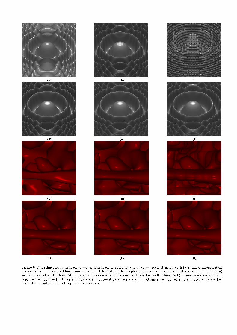
extent they are impracticable. Simple truncation causessevere ringing artifacts, as can be seen in Fig. 6, whichshows the Marschner-Lobb data set [6] reconstructed withlinear interpolation and central di�erences and linear inter-polation (Fig. 6a), the Catmull-Rom spline and derivative(Fig. 6b) and the truncated cosc of width three (Fig. 6c).(for high resolution images please refer to the web page ofthis project [15]). We will investigate and explain the causeof this bad result in frequency domain in Chapter 3 and inspatial domain in Chapter 4.To reduce artifacts originating from truncation the ideal

reconstruction �lters can be multiplied with appropriatefunctions which drop o� more smoothly at the edges. We willdiscuss some of the more commonly used of these functions,which are adversely called windows. We show that most ofthem are unsuitable for reconstruction, especially for higherorder derivative reconstruction, although some, for exampleHamming [5] and Lanczos [16] windows, are reported to becommonly used.

2 Previous work

Turkowski [16] used windowed sinc functions for image re-sampling. He found the Lanczos window superior in termsof reduction of aliasing, sharpness, and minimal ringing asconclusion of an empirical experiment.Marschner and Lobb [6] used a cosine-bell windowed sinc

(often called Hann window) and found it superior to the en-tire family of cubic reconstruction �lters. According to theirmetric there is always a windowed sinc with better smooth-ing and post-aliasing properties. Machiraju and Yagel [5]use a Hamming windowed sinc without further explanationof their choice. However, we found the Hamming windowof not being optimal. Recently, Meijering et al. [7] per-formed a purely quantitative comparison of eleven windowedsinc functions. They found the Welch, Cosine, Lanczos andKaiser windows yielding the best results and noted that thetruncated sinc was one of the worst performing reconstruc-tion �lters.Goss [2] extended the idea of windowing the ideal recon-

struction �lter to derivative reconstruction. The parameterof the Kaiser window controls the smoothing characteristics

of the reconstructed function. Goss uses the windowed cosconly on sampling points, in between some interpolation hasto be performed which is not stated explicitly.Most researchers assess the quality of reconstruction �lters

in frequency domain, whereas M�oller et. al [10] propose apurely numerical method operating in spatial domain. Wewill review this method in Chapter 4 as it will allow us toderive optimal parameters, in terms of numerical accuracy,for the Kaiser and Gaussian windows.

3 Windowing ideal reconstruction �lters

The windows investigated in this work are

- The rectangular window or box function

��(x) =

�1 if jxj � �

0 else(3)

which performs pure truncation.

- The Bartlett window, which is actually just a tent func-tion:

Bartlett� (x) =

�1� jxj

�if jxj < �

0 else(4)

- The Welch window:

Welch� (x) =

�1�

�x

�

�2 jxj < �

0 else(5)

- The Parzen window

Parzen(x) =1

4

(4� 6jxj2 + 3jxj3 0 � jxj < 1

(2� jxj)3 1 � jxj < 20 else

(6)is a piece-wise cubic approximation of the Gaussianwindow with extend two. Although its width is notdirectly adjustable it can, of course, be scaled to everydesired extend.

- The Hann window (due to Julius van Hann, oftenwrongly referred to as Hanning window [17], sometimesjust cosine bell window) and Hamming window, whichare quite similar, they only di�er in the choice of oneparameter �:

H�;�(x) =

��+ (1� �) cos(� x

�) jxj < �

0 else(7)

with � = 1

2being the Hann window and � = 0:54 the

Hamming Window.

- The Blackman window, which has one additional cosineterm as compared to the Hann and Hamming window.

Blackman� (x) =

(0:42 + 1

2cos(� x

�)+

0:08 cos(2� x

�) jxj < �

0 else

(8)

- The Lanczos window, which is the central lobe of a sincfunction scaled to a certain extend.

Lanczos� (x) =

�sin(�

x

�)

�x

�

jxj < �

0 else(9)

spatialdomain

-0.2

0

0.2

0.4

0.6

0.8

1

1.2

-3 -2 -1 0 1 2 3

rectangular windowBartlett windowWelch window

Parzen window

-0.2

0

0.2

0.4

0.6

0.8

1

1.2

-3 -2 -1 0 1 2 3

Hann windowHamming windowBlackman window

Lanczos window

frequencydomain

0

0.2

0.4

0.6

0.8

1

1.2

pi

rectangular windowed sincBartlett windowed sincWelch windowed sinc

Parzen windowed sincideal

0

0.2

0.4

0.6

0.8

1

1.2

pi

Hann windowed sincHamming windowed sincBlackman windowed sinc

Lanczos windowed sincideal

0

0.5

1

1.5

2

2.5

3

3.5

00 pi 2pi

rectangular windowed coscBartlett windowed coscWelch windowed cosc

Parzen windowed coscideal

0

0.5

1

1.5

2

2.5

3

3.5

00 pi 2pi

Hann windowed coscHamming windowed coscBlackman windowed cosc

Lanczos windowed coscIdeal

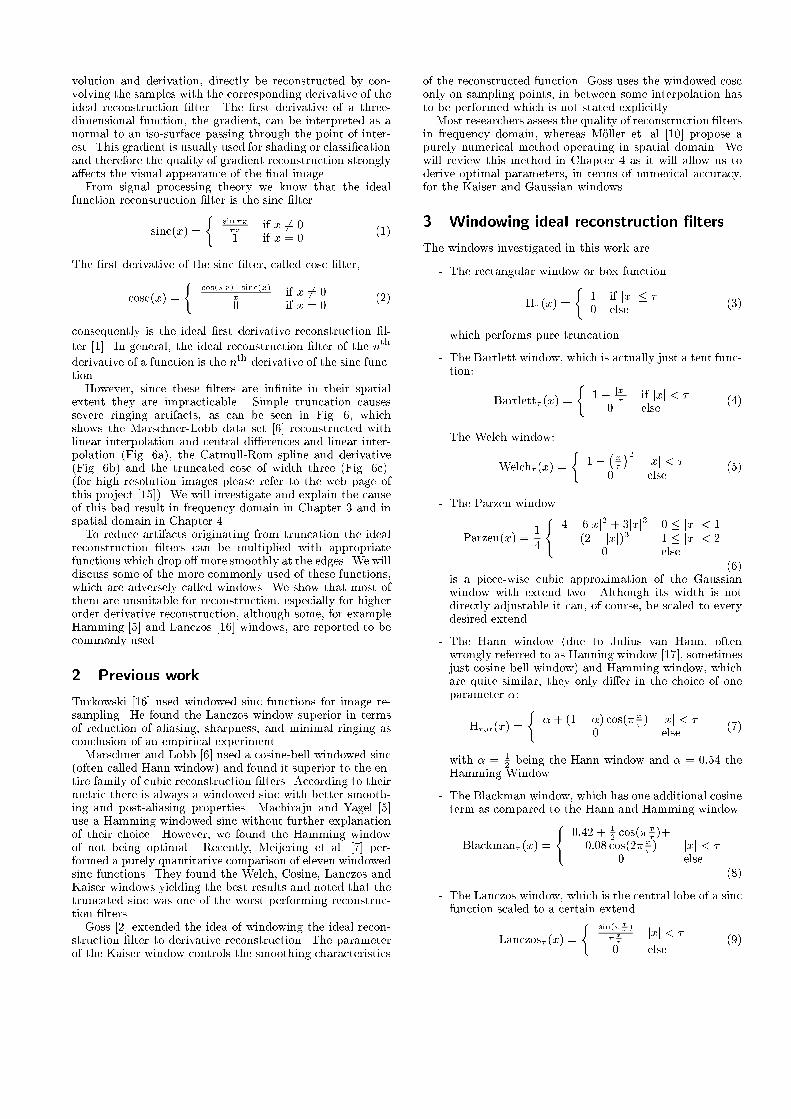
Figure 2: Rectangular, Bartlett, Welch, Parzen, Hann, Hamming, Blackman and Lanczos windows of width two on top, belowthe frequency responses of correspondingly windowed sinc and cosc functions.

- The Kaiser window [3], which has an adjustable param-eter � which controls how steeply it approaches zero atthe edges. It is de�ned by

Kaiser�;�(x) =

(I0(�

p1�(x=�)2)

I0(�)jxj � �

0 else(10)

where I0(x) is the zeroth order modi�ed Bessel func-tion [13]. The higher � gets the narrower becomes theKaiser window.

- and we can also use a truncated Gaussian function as

window. It is in its general form de�ned by

Gauss�;�(x) =

�2�(

x

�)2 jxj < �

0 else(11)

with � being the standard deviation. The higher �

gets, the wider the Gaussian window becomes and, onthe other hand, the more severe gets the truncation.

All these windows, except Kaiser and Gaussian windows, aredepicted in Fig. 2 on top, the frequency responses of corre-spondingly windowed sinc (with window width two) in themiddle row and windowed cosc in the bottom row. Sincefunction reconstruction �lters are even functions and �rstderivative �lters are odd functions, the power spectra, as

spatialdomain

-0.2

0

0.2

0.4

0.6

0.8

1

1.2

-3 -2 -1 0 1 2 3

Kaiser window alpha=2alpha=4alpha=8

alpha=16

-0.2

0

0.2

0.4

0.6

0.8

1

1.2

-3 -2 -1 0 1 2 3

Gaussian window sigma=1.0sigma=1.5sigma=1.8sigma=2.0

frequencydomain

0

0.2

0.4

0.6

0.8

1

1.2

pi

Kaiser windowed sinc alpha=2alpha=4alpha=8

alpha=16ideal

0

0.2

0.4

0.6

0.8

1

1.2

pi

Gaussian windowed sinc sigma=1.0sigma=1.5sigma=1.8sigma=2.0

ideal

0

0.5

1

1.5

2

2.5

3

3.5

4

00 pi 2pi

Kaiser windowed cosc alpha=2alpha=4alpha=8

alpha=16Ideal

0

0.5

1

1.5

2

2.5

3

3.5

00 pi 2pi

Gaussian windowed cosc sigma=1.0sigma=1.5sigma=1.8sigma=2.0

Ideal

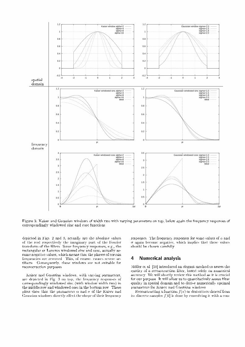
Figure 3: Kaiser and Gaussian windows of width two with varying parameters on top, below again the frequency responses ofcorrespondingly windowed sinc and cosc functions.

depicted in Figs. 2 and 3, actually are the absolute valuesof the real respectively the imaginary part of the Fouriertransform of the �lters. Some frequency responses, e.g., therectangular or Lanczos windowed sinc and cosc, actually as-sume negative values, which means that the phases of certainfrequencies are reverted. This, of course, causes severe ar-tifacts. Consequently, these windows are not suitable forreconstruction purposes.

Kaiser and Gaussian windows, with varying parameters,are depicted in Fig. 3 on top, the frequency responses ofcorrespondingly windowed sinc (with window width two) inthe middle row and windowed cosc in the bottom row. Theseplots show that the parameters � and � of the Kaiser andGaussian windows directly a�ect the shape of their frequency

responses. The frequency responses for some values of � and� again become negative, which implies that these valuesshould be chosen carefully.

4 Numerical analysis

M�oller et al. [10] introduced an elegant method to assess thequality of a reconstruction �lter, based solely on numericalaccuracy. We will shortly review this method as it is crucialfor our purpose. It will allow us to quantitatively assess �lterquality in spatial domain and to derive numerically optimalparameters for Kaiser and Gaussian windows.Reconstructing a function f(x) or derivatives thereof from

its discrete samples f [k] is done by convolving it with a con-

-0.1

-0.05

0

0.05

0.1

0 0.2 0.4 0.6 0.8 1

truncatedBartlett windowedWelch windowed

Parzen windowed

-0.1

-0.05

0

0.05

0.1

0 0.2 0.4 0.6 0.8 1

HannHamming windowedBlackman windowed

Lanczos windowed

-0.1

-0.05

0

0.05

0.1

0 0.2 0.4 0.6 0.8 1

Kaiser windowed with alpha=2alpha=4alpha=8

alpha=16

-0.1

-0.05

0

0.05

0.1

0 0.2 0.4 0.6 0.8 1

Gaussian windowed with sigma=1.0sigma=1.5sigma=1.8sigma=2.0

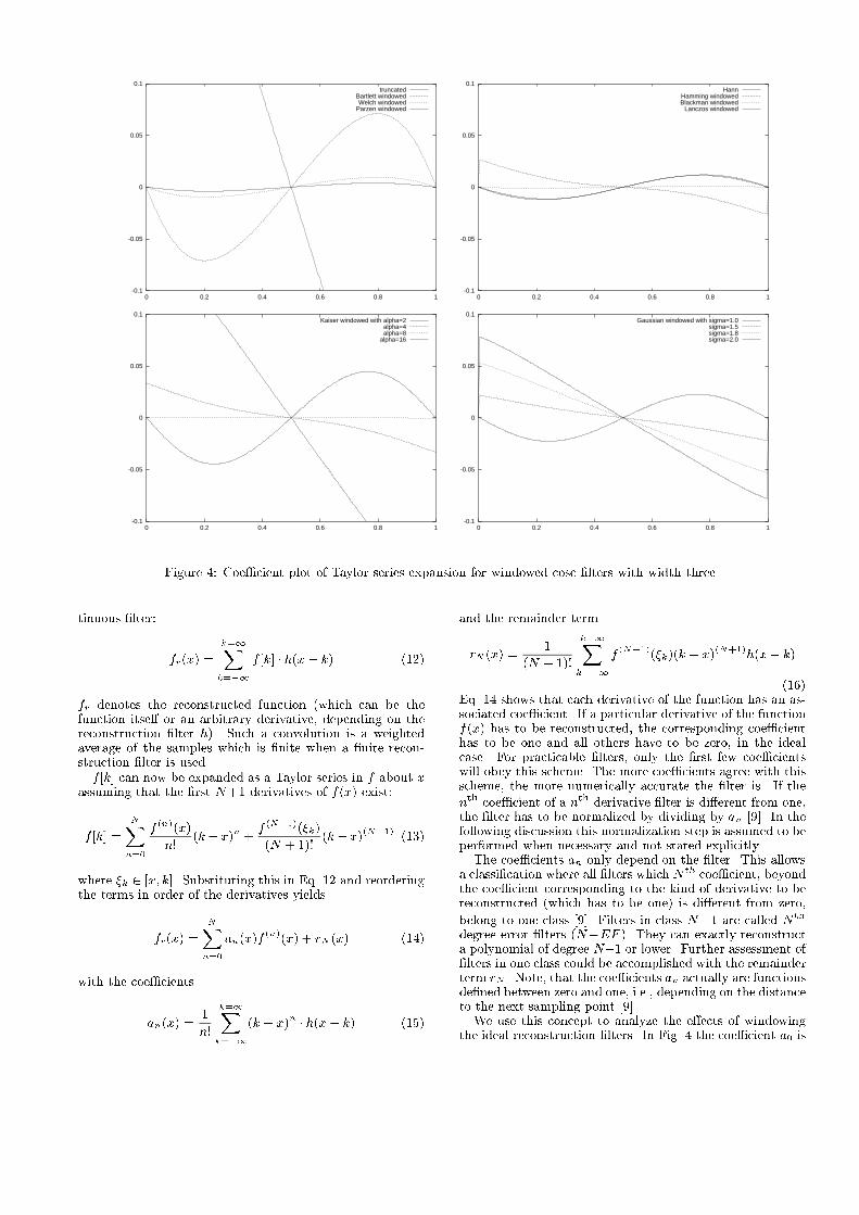
Figure 4: Coe�cient plot of Taylor series expansion for windowed cosc �lters with width three.

tinuous �lter:

fr(x) =

k=1Xk=�1

f [k] � h(x� k) (12)

fr denotes the reconstructed function (which can be thefunction itself or an arbitrary derivative, depending on thereconstruction �lter h). Such a convolution is a weightedaverage of the samples which is �nite when a �nite recon-struction �lter is used.

f [k] can now be expanded as a Taylor series in f about xassuming that the �rst N+1 derivatives of f(x) exist:

f [k] =

NXn=0

f(n)(x)

n!(k� x)

n+f(N+1)(�k)

(N + 1)!(k� x)

(N+1)(13)

where �k 2 [x; k]. Substituting this in Eq. 12 and reorderingthe terms in order of the derivatives yields

fr(x) =

NXn=0

an(x)f(n)

(x) + rN (x) (14)

with the coe�cients

an(x) =1

n!

k=1Xk=�1

(k � x)n � h(x� k) (15)

and the remainder term

rN (x) =1

(N + 1)!

k=1Xk=�1

f(N+1)

(�k)(k � x)(N+1)

h(x� k)

(16)Eq. 14 shows that each derivative of the function has an as-sociated coe�cient. If a particular derivative of the functionf(x) has to be reconstructed, the corresponding coe�cienthas to be one and all others have to be zero, in the idealcase. For practicable �lters, only the �rst few coe�cientswill obey this scheme. The more coe�cients agree with thisscheme, the more numerically accurate the �lter is. If the

nth coe�cient of a nth derivative �lter is di�erent from one,

the �lter has to be normalized by dividing by an [9]. In thefollowing discussion this normalization step is assumed to beperformed when necessary and not stated explicitly.The coe�cients an only depend on the �lter. This allows

a classi�cation where all �lters which N th coe�cient, beyondthe coe�cient corresponding to the kind of derivative to bereconstructed (which has to be one) is di�erent from zero,

belong to one class [9]. Filters in class N�1 are called Nth

degree error �lters (N�EF ). They can exactly reconstructa polynomial of degree N�1 or lower. Further assessment of�lters in one class could be accomplished with the remainderterm rN . Note, that the coe�cients an actually are functionsde�ned between zero and one, i.e., depending on the distanceto the next sampling point [9].We use this concept to analyze the e�ects of windowing

the ideal reconstruction �lters. In Fig. 4 the coe�cient a0 is

0

0.5

1

1.5

2

2.5

3

3.5

4

0 2 4 6 8 10 12

||an(

x)||

alpha

sinc (a1)cosc (a0)

0

0.05

0.1

0.15

0.2

0.25

0.3

0.35

0.4

0.45

0.5

3 3.5 4 4.5 5 5.5 6 6.5 7

||an(

x)||

alpha

sinc (a1)cosc (a0)

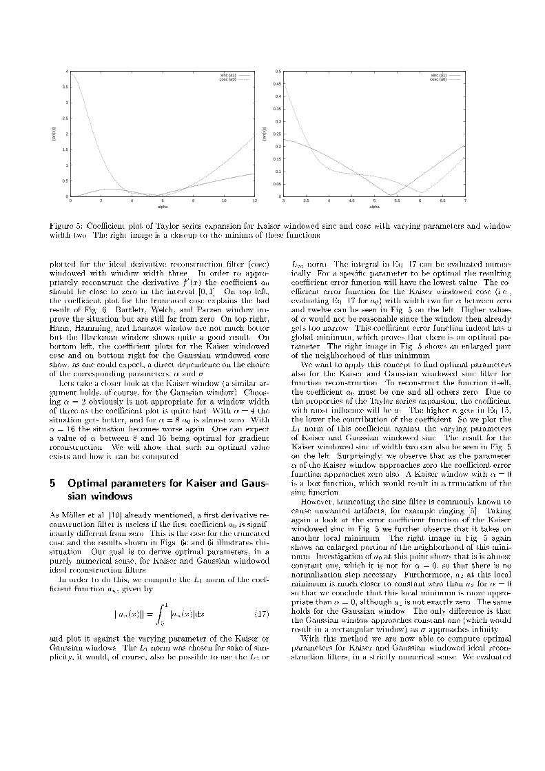
Figure 5: Coe�cient plot of Taylor series expansion for Kaiser windowed sinc and cosc with varying parameters and windowwidth two. The right image is a closeup to the minima of these functions.

plotted for the ideal derivative reconstruction �lter (cosc)windowed with window width three. In order to appro-priately reconstruct the derivative f

0(x) the coe�cient a0

should be close to zero in the interval [0; 1]. On top left,the coe�cient plot for the truncated cosc explains the badresult of Fig. 6. Bartlett, Welch, and Parzen window im-prove the situation but are still far from zero. On top right,Hann, Hamming, and Lanczos window are not much betterbut the Blackman window shows quite a good result. Onbottom left, the coe�cient plots for the Kaiser windowedcosc and on bottom right for the Gaussian windowed coscshow, as one could expect, a direct dependence on the choiceof the corresponding parameters, � and �.

Lets take a closer look at the Kaiser window (a similar ar-gument holds, of course, for the Gaussian window). Choos-ing � = 2 obviously is not appropriate for a window widthof three as the coe�cient plot is quite bad. With � = 4 thesituation gets better, and for � = 8 a0 is almost zero. With� = 16 the situation becomes worse again. One can expecta value of � between 8 and 16 being optimal for gradientreconstruction. We will show that such an optimal valueexists and how it can be computed.

5 Optimal parameters for Kaiser and Gaus-

sian windows

As M�oller et al. [10] already mentioned, a �rst derivative re-construction �lter is useless if the �rst coe�cient a0 is signif-icantly di�erent from zero. This is the case for the truncatedcosc and the results shown in Figs. 6c and 6i illustrates thissituation. Our goal is to derive optimal parameters, in apurely numerical sense, for Kaiser and Gaussian windowedideal reconstruction �lters.

In order to do this, we compute the L1 norm of the coef-�cient function an, given by

jjan(x)jj =Z

1

0

jan(x)jdx (17)

and plot it against the varying parameter of the Kaiser orGaussian windows. The L1 norm was chosen for sake of sim-plicity, it would, of course, also be possible to use the L2 or

L1 norm. The integral in Eq. 17 can be evaluated numer-ically. For a speci�c parameter to be optimal the resultingcoe�cient error function will have the lowest value. The co-e�cient error function for the Kaiser windowed cosc (i.e.,evaluating Eq. 17 for a0) with width two for � between zeroand twelve can be seen in Fig. 5 on the left. Higher valuesof � would not be reasonable since the window then alreadygets too narrow. This coe�cient error function indeed has aglobal minimum, which proves that there is an optimal pa-rameter. The right image in Fig. 5 shows an enlarged partof the neighborhood of this minimum.We want to apply this concept to �nd optimal parameters

also for the Kaiser and Gaussian windowed sinc �lter forfunction reconstruction. To reconstruct the function itself,the coe�cient a0 must be one and all others zero. Due tothe properties of the Taylor series expansion, the coe�cientwith most in uence will be a1. The higher n gets in Eq 15,the lower the contribution of the coe�cient. So we plot theL1 norm of this coe�cient against the varying parametersof Kaiser and Gaussian windowed sinc. The result for theKaiser windowed sinc of width two can also be seen in Fig. 5on the left. Surprisingly, we observe that as the parameter� of the Kaiser window approaches zero the coe�cient errorfunction approaches zero also. A Kaiser window with � = 0is a box function, which would result in a truncation of thesinc function.However, truncating the sinc �lter is commonly known to

cause unwanted artifacts, for example ringing [5]. Takingagain a look at the error coe�cient function of the Kaiserwindowed sinc in Fig. 5 we further observe that it takes onanother local minimum. The right image in Fig. 5 againshows an enlarged portion of the neighborhood of this mini-mum. Investigation of a0 at this point shows that is is almostconstant one, which it is not for � = 0, so that there is nonormalization step necessary. Furthermore, a2 at this localminimum is much closer to constant zero than a2 for � = 0so that we conclude that this local minimum is more appro-priate than � = 0, although a1 is not exactly zero. The sameholds for the Gaussian window. The only di�erence is thatthe Gaussian window approaches constant one (which wouldresult in a rectangular window) as � approaches in�nity.With this method we are now able to compute optimal

parameters for Kaiser and Gaussian windowed ideal recon-struction �lters, in a strictly numerical sense. We evaluated

Window width2 3 4 5

function reconstruction (sinc) �(Kaiser window) 5.36 8.93 12.15 15.4�(Gaussian window) 1.11 1.33 1.46 1.63

�rst derivative reconstruction (cosc) �(Kaiser window) 6.05 9.28 12.5 15.5�(Gaussian window) 1.045 1.238 1.42 1.56

Table 1: Optimal values for the parameters for Kaiser and Gaussian windows for function and �rst derivative reconstructionwith window width two, three, four, and �ve.

values for Kaiser and Gaussian windowed sinc and cosc ofwindow width two, three, four and �ve, which are presentedin Table 1. Not re ected in this table is the fact that theabsolute numerical error is one magnitude smaller for theKaiser windowed ideal reconstruction �lters as compared tothe Gaussian or Blackman windowed ideal reconstruction�lters.

6 Results

To evaluate the results of the last chapters we �rst tested thereconstruction �lters on a standard arti�cial data set pro-posed by Marschner and Lobb [6]. We used our framework\Smurf: a smart surface model for advanced visualizationtechniques" [4] which easily allows to replace reconstruction�lters. We used a ray-casting iso-surface extraction algo-rithm and always used the �rst derivative of the functionreconstruction �lter also for �rst derivative reconstruction.This is according to the scheme proposed by Bentum et al. [1](with the exception of linear interpolation, where central dif-ferences with linear interpolation were used).Fig. 6a shows the result for central di�erences and linear

interpolation. We clearly observe the smoothing, which isan intrinsic property of this method [2], as the image is toobright. In Fig. 6b, the Catmull-Rom spline and its derivative(i.e., a BC-Spline with B = 0 and C = 0:5 [8] or, equiva-lently, a cardinal spline with a = �0:5 [1]) were used. We seethat the smoothing is reduced but the structure of the arti-facts remains. In Fig. 6c truncated sinc and cosc were used.This image shows practically what was discussed theoreti-cally in Chapters 3 and 4. Truncating ideal reconstruction�lters is more or less useless.Figs. 6d { 6f shows images reconstructed with the sinc

and cosc �lter windowed with the more promising windowsfrom our numerical analysis in Chapter 4. Fig. 6d shows theBlackman window, which is �xed for a certain width (weused a window width of three for this image). The Black-man window gives already quite a good behavior. In Fig. 6ea Kaiser window of width three was used with � = 8:93 forfunction reconstruction and � = 9:28 for �rst derivative re-construction, according to Table 1, which further reduces theannoying artifacts present in the previous reconstructions.A Gaussian window of width three with numerically opti-mal parameters (� = 1:33 for function reconstruction and� = 1:238 for �rst derivative reconstruction) shows some ar-tifacts, especially visible in the highlights, again. This is dueto the fact that a window width of three is too narrow forthe Gaussian window [14].The �lters were also tested on real world data sets, such

as a CT scan of a human head and an MR scan of a hu-man kidney. Figs. 6g { 6l show the results for a close-up ofthe kidney data set. The same reconstruction �lters wereused in the same order as for the Marschner-Lobb data setabove. Figs. 6g and 6i show again the de�ciencies of linear in-

terpolation and central di�erences with linear interpolationand truncated sinc and cosc. Cubic splines (Fig. 6h) showsome artifacts especially in the highlights which are removedby the Blackman and Kaiser window (Figs. 6j and 6k).The Gaussian window again introduces artifacts, also, quitenotable, in the function reconstruction, due to the windowwidth of three.Fig. 1 shows the results for the head data set. Linear

interpolation for function reconstruction and central di�er-ences with linear interpolation for gradient reconstructionwere used in the left image. We see that this method in-troduces quite some smoothing, so that the skull appearsquite smooth and visually appealing. However, the close-upbelow shows that it is not suitable for reconstructing smallfeatures. In the middle the Catmull-Rom spline was usedboth for function reconstruction and gradient reconstruc-tion. We see that the skull exhibits stair case artifacts asthey are not smoothed out any more but the close-up clearlyexhibits the better reconstruction quality of this �lter. Onthe right we used Kaiser windowed sinc and cosc with win-dow width three and numerically optimal parameters. Herewe can see the better reconstruction especially as the high-lights in the close-up appear more sharply. Again, the skullexhibits stair-case artifacts which actually are a visualizationof data accuracy. Although the result with central di�er-ences is visually more appealing, the Kaiser windowed sincand cosc are physically more correct.For further images (also of the other not so good perform-

ing windows) please refer to earlier work of the authors [14]and to the web page of this project [15].

7 Conclusions and Future Work

We showed that windowing ideal reconstruction �lters al-lows to improve reconstruction quality as compared to thethe use of traditional reconstruction methods like linear in-terpolation or cubic splines. Windowing ideal reconstruction�lters also has the advantage that better reconstruction canbe achieved by using wider windows, which, however, alsoincreases the computational cost.From the comparison of some of the more commonly used

windows we conclude that the choice of the windowing func-tion is crucial. We showed that some popular windows, likethe Lanczos or Hamming window, are not optimal in thesense of numerical accuracy. From our experiments as wellas from numerical analysis we found Blackman, Kaiser andGaussian windows performing best.Further, we derived numerical optimal values for Kaiser

and Gaussian windows, which have a parameter to controltheir shape. Our analysis of ideal reconstruction �lters win-dowed with these windows using a Taylor series expansion ofthe convolution sum allowed us to determine optimal valuesfor the parameters of these windows, in a strictly numeri-cal sense. The Kaiser window performs best in this regard

as the numerical error is smallest. As the Gaussian win-dows shows some de�ciencies for a window width of three,we conclude that the Blackman window is a �rst good choicewhich, however, can be improved by using a Kaiser windowwith numerically optimal parameters.

Continuity conditions, which are very important for thevisual appearance of the resulting image [11] have not beenaddressed and are left for future work. Our experimentsshowed also that a coupling of function reconstruction andderivative reconstruction improves over-all reconstructionquality. This area deserves further investigation, probablyin a way similar to Neumann et al. [12] who use a tight cou-pling of function and gradient reconstruction based on linearregression.

8 Acknowledgments

The work presented in this paper has been funded by theVisMed project (http://www.vismed.at/). VisMed is sup-ported by Tiani Medgraph , Vienna (http://www.tiani.com/) and the Forschungsf�orderungsfonds f�ur die gewerblicheWirtschaft, Austria (http://www.telecom.at/fff/). Themedical data sets are courtesy of Tiani Medgraph GesmbH,Vienna. Special thanks go to Ji�r�� Hlad�uvka, Jan P�rikryl andRobert F. Tobler for proof reading and valuable hints anddiscussions.

References

[1] M. J. Bentum, B. B. A. Lichtenbelt, and T. Malzbender.Frequency Analysis of Gradient Estimators in VolumeRendering. IEEE Transactions on Visualization andComputer Graphics, 2(3):242{254, September 1996.

[2] M. E. Goss. An adjustable gradient �lter for volumevisualization image enhancement. In Proceedings ofGraphics Interface '94, pages 67{74, Ban�, Alberta,Canada, May 1994. Canadian Information ProcessingSociety.

[3] J. F. Kaiser and R. W. Schafer. On the Use ofthe I0-Sinh Window for Spectrum Analysis. IEEETrans. Acoustics, Speech and Signal Processing, ASSP-28(1):105, 1980.

[4] H. L�o�elmann, T. Theu�l, A. K�onig, and M. E. Gr�oller.Smurf: a smart surface model for advanced visualiza-tion techniques. In Winter School of Computer Graph-ics '99, pages 156 { 164, Plzen, Czech Republic, 1999.To appear revised as "Smart surface interrogation foradvanced visualization techniques" in journal of HighPerformance Computer Graphics, April/May 2000.

[5] R. Machiraju and R. Yagel. Reconstruction errorcharacterization and control: A sampling theory ap-proach. IEEE Transactions on Visualization and Com-puter Graphics, 2(4):364{378, December 1996.

[6] S. R. Marschner and R. J. Lobb. An evaluation of re-construction �lters for volume rendering. In R. DanielBergeron and Arie E. Kaufman, editors, Proceedingsof the Conference on Visualization, pages 100{107, LosAlamitos, CA, USA, October 1994. IEEE Computer So-ciety Press.

[7] E. H. W. Meijering, W. J. Niessen, J. P. W. Pluim,and M. A. Viergever. Quantitative comparison of sinc-approximating kernels for medical image interpolation.In C. Taylor and A. Colchester, editors, Medical Im-age Computing and Computer Assisted Intervention -MICCAI'99, pages 210{217, September 1999.

[8] D. P. Mitchell and A. N. Netravali. Reconstruc-tion �lters in computer graphics. Computer Graphics,22(4):221{228, August 1988.

[9] T. M�oller, R. Machiraju, K. M�uller, and R. Yagel. Clas-si�cation and local error estimation of interpolation andderivative �lters for volume rendering. In Proceedings1996 Symposium on Volume Visualization, pages 71{78,September 1996.

[10] T. M�oller, R. Machiraju, K. M�uller, and R. Yagel. Eval-uation and Design of Filters Using a Taylor Series Ex-pansion. IEEE Transactions on Visualization and Com-puter Graphics, 3(2):184{199, 1997.

[11] T. M�oller, K. M�uller, Y. Kurzion, Raghu Machiraju,and Roni Yagel. Design of accurate and smooth �ltersfor function and derivative reconstruction. In IEEESymposium on Volume Visualization, pages 143{151.IEEE, ACM SIGGRAPH, 1998.

[12] L. Neumann, B. Cs�ebfalvi, A. K�onig, and M. E. Gr�oller.Gradient estimation in volume data using 4D linear re-gression. Technical Report TR-186-2-00-03, Institute ofComputer Graphics, Vienna University of Technology,2000. Accepted for EUROGRAPHICS 2000.

[13] W. H. Press, B. P. Flannery, S. A. Teukolsky, and W. T.Vetterling. Numerical Recipes in C: The Art of Scien-ti�c Computing. Cambridge UP, 1988.

[14] T. Theu�l. Sampling and reconstruction in volume visu-alization. Master's thesis, Vienna University of Technol-ogy, 2000. http://www.cg.tuwien.ac.at/~theussl/

DA/.

[15] T. Theu�l, H. Hauser, and M. E. Gr�oller. Mas-tering windows: Improving reconstruction { webpage. http://www.cg.tuwien.ac.at/research/vis/

vismed/Windows/.

[16] K. Turkowski. Filters for common resampling tasks.In Andrew S. Glassner, editor, Graphics Gems I, pages147{165. Academic Press, 1990.

[17] G. Wolberg. Digital Image Warping. IEEE ComputerSociety Press, 10662 Los Vaqueros Circle, Los Alamitos,CA, 1990. IEEE Computer Society Press Monograph.

(a) (b) (c)

(d) (e) (f)

(g) (h) (i)

(j) (k) (l)

Figure 6: Marschner Lobb data set (a { f) and data set of a human kidney (g { l) reconstructed with (a,g) linear interpolationand central di�erences and linear interpolation, (b,h) Catmull-Rom spline and derivative, (c,i) truncated (rectangular window)sinc and cosc of width three, (d,j) Blackman windowed sinc and cosc with window width three, (e,k) Kaiser windowed sinc andcosc with window width three and numerically optimal parameters and (f,l) Gaussian windowed sinc and cosc with windowwidth three and numerically optimal parameters.