Autonomous Cruise Control for Chalmers Vehicle...
88
Autonomous Cruise Control for Chalmers Vehicle Simulator Design and Implementation PÄR BERGGREN Department of Signals and Systems CHALMERS UNIVERSITY OF TECHNOLOGY Göteborg, Sweden 2008 Master Thesis: EX047/2008
-
Upload
truongdieu -
Category
Documents
-
view
217 -
download
0
Transcript of Autonomous Cruise Control for Chalmers Vehicle...

Autonomous Cruise Control for Chalmers Vehicle SimulatorDesign and Implementation
PÄR BERGGREN
Department of Signals and SystemsCHALMERS UNIVERSITY OF TECHNOLOGYGöteborg, Sweden 2008Master Thesis: EX047/2008


MASTER THESIS: EX047/2008
Autonomous Cruise Control for Chalmers Vehicle SimulatorDesign and Implementation
Author: Pär Berggren
Examiner: Senior Lecturer Jonas Fredriksson
Department of Signals and Systems CHALMER UNIVERSITY OF TECHNOLOGY
Göteborg, Sweden 2008.
Autonomous Cruise Control for Chalmers Vehicle SimulatorDesign and ImplementationPÄR BERGGREN
© PÄR BERGGREN, 2008.
Master Thesis: EX047/2008Department of Signals and SystemsChalmers University of TechnologySE - 412 96 GöteborgSwedenTelephone + 46 (0)31-772 1000
Cover:A combination of a simulation model of the closed loop system when using the suggested control approch, see page 34, together with an illustration of the accepting range of the virtual radar sensor developed in this paper, see page 19.
Department of Signals and Systems Göteborg, Sweden 2008.

Autonomous Cruise Control for Chalmers Vehicle SimulatorDesign and Implementation
PÄR BERGGRENDepartment of Signals and SystemsChalmers University of Technology
ABSTRACT
In this thesis an Autonomous Cruise Control for a vehicle simulator is designed and implemented. Autonomous Cruise Control is a type of cruise control based on distance keeping as opposed to velocity keeping. In order to establish realtime communication over an existing CAN-bus the program dealing with this was remodelled and changes to the program was implemented. In order to allow feedback of the distance to and velocity of a leading vehicle, a plug-in to the vehicle simulator´s graphics program was created. A cascaded PID controller was designed and compared with a controller taken from litterature. Simulations suggest that these controllers are comparable in certain simulated safety aspects.
Keywords: Autonomous Cruise Control, Chalmers Vehicle Simulator, radar, gray-box model, step response, residual analysis, PID controller, emergency stopping, cut-in situations, CAN-bus, realtime communication.


Table of Contents
Chapter 1 Introduction........................................................................................................................11.1 Autonomous Cruise Control...................................................................................................... 11.2 Thesis goal ................................................................................................................................ 21.3 Thesis scope...............................................................................................................................31.4 Chalmers Vehicle Simulator......................................................................................................4
Chapter 2 CAN-bus communication................................................................................................... 92.1 A brief introduction to the CAN-bus......................................................................................... 92.2 Probem description.................................................................................................................. 112.3 Current algorithm.....................................................................................................................112.4 Remodelled CAN communication...........................................................................................13
Chapter 3 Sensor development..........................................................................................................173.1 The graphics environment....................................................................................................... 173.2 The radar sensor ......................................................................................................................19
Chapter 4 System modelling ............................................................................................................ 234.1 Model synthesis....................................................................................................................... 23
4.1.1 Experiment and data collection........................................................................................244.1.2 Modelling......................................................................................................................... 25
4.2 Model verification....................................................................................................................284.2.1 Model benchmarking....................................................................................................... 28
4.3 Model completion and noise sources.......................................................................................31
Chapter 5 Control Design..................................................................................................................335.1 Control loop formulation......................................................................................................... 335.2 Control synthesis and approach analysis................................................................................. 36
5.2.1 Distance feedback............................................................................................................ 385.2.2 Distance and speed difference feedback.......................................................................... 425.2.3 A benchmarking controller ............................................................................................. 485.2.4 Simulations of stopping and cut-ins ................................................................................51
Chapter 6 Implementations................................................................................................................556.1 Offline simulator .....................................................................................................................556.2 Online simulator...................................................................................................................... 58
Chapter 7 Discussion, future work and conclusions......................................................................... 637.1 Discussion ...............................................................................................................................63
7.1.1 Future work...................................................................................................................... 667.2 Conclusions..............................................................................................................................67

List of Symbols
k Sample index.M Sample horizon.N Number of samples.
s Laplacian variable (Complex frequency).t [s] Time.τ [s] Time; variable.
ω [s-1] Frequency.
Control: a(t) [m / s] Acceleration. Am Gain margin. b( x , x ) The uncontrollable part of the acceleration dynamics of a
car. c Constant; Df over (KP KD). c(t) Designable part of the AICC controller. CP Feedback gain of distance for AICC. CV Feedback of vehicle velocity. d [m] Distance variable. Df Derivation filter time. dm( x ) [kg m / s2 ] Mechanical drag of car. e Control error. eD Distance error. eV Velocity error. Ka Feedback of vehicle acceleration. KD Derivation gain. kd [kg / m] Aerodynamic drag of car. KI Integration gain. KP Proportional gain. Kv Velocity gain. Kv Feedback gain of velocity (difference). m [kg] Mass of vehicle. N Number of circulations around minus one. P Number of poles in the right half-plane of the complex
plane. R Radius of halfcircle and refence value in Laplace plane.

r [-] Radius of halfcircle and reference value. S0 [m] Minimum safe distance, used in AICC. t5% [s] Settling time. u(t) Control signal. v(t) [m / s] Velocity. vD [m / s] Velocity difference. vl [m / s] Velocity of leading vehicle. w Measurement noise. x [m] Position of your car.x [m / s] Velocity, time derivative of position.x [m / s2] Acceleration, second time derivative of position.
Z Number of zero crossings in right half-plane of complex plane.
x [(kg s)-1] Function multiplied to throttle in AICC.
δ(t) [m] The safety distance policy in AICC. θ [rad] Angle. λ [s-1] The gain of the velocity when added to the safety distance
policy from AICC.
x [s] Time constant of engine.
φm [°] Phase margin.
Transfer functions:F The controller without integration.
F The controller. G General process model. Gdu Model of the process d over u. Gdvl Model of the process d over vl. Gm Model of a “real” process. L The loop of a feedback control system. Ld The loop; broken up at the distance signal. Lu The loop; broken up at the control signal.

Modelling: Pr Variance of predicted crosscovariance function. Ru(k) Covariance function of input signal. Rε(k) Covariance function of predicted error.Rεuτ Predicted crosscovariance function.
u(t) Input signal. y(t) Output signal.
yt∣θN Prediction of system output signal.
ε(t) Prediction error.θN
Estimated model parameters.
Automata:QP The finite set of state-names of automaton P.
P The alphabet of automaton P.
iP The initial state of automaton P.
P The transition function of automata P.
Table 1: Prefixes for Binary Mulitiples. According to (Nordling, Österman, 2004) in part CU, chapter 2.6 on page 23.Factor Name Symbol2^10 kibi Ki2^20 mebi Mi2^30 gibi Gi2^40 tebi Ti2^50 pebi Pi2^60 exbi Ei

Chapter 1
Introduction
HE FIRST PART of this introductory chapter consists of a short introduction to Autonomous Cruise Control and then
an introduction to the Chalmers Vehicle Simulator (CVS) itself is presented. Finally the goal and scope of the thesis are presented. The two next coming chapters deals with signal routing (the CAN-bus) and sensor creation. The two thereafter following chapters deals with modelling and control design. The chapter coming after those presents and discusses the implementations done in the Simulink model used in the vehicle simulator and in the last chapter discussions, future work and conclusions are brought up.
T
1.1 Autonomous Cruise Control
AUTONOMOUS CRUISE CONTROL or ACC for short is a term used in this paper to describe a cruise control based on distance keeping. In the litterature this has almost as many names and variations as there are researchers in the field. Examples of the variations of names can be Adaptive Cruise Control and Autonomous Intelligent Cruise Control.
1

2 Chapter 1 Introduction
The name used here is chosen to minimize the confusion of the reader and in order not imply that the ACC designed in this paper is of adaptive type (no parameter is changed by the control algorithm) or some type of machine intelligence.
An ACC is basically a Cruise Control taken a step further, so that instead of using a velocity feedback (from the speedometer) to maintain a preset speed, feedback of distance to and velocity of a leading vehicle is created in order to maintain a safe distance, see for instance (Iuanno, 1993). The feedback needed for an ACC is usually created using a radar but other sensors can also be used. For instance one can use GPS and communicate information about velocity and position to other vehicles over a wireless connection.
1.2 Thesis goal
THE GOAL OF this thesis is primarily to design an Autonomous Cruise Control for use on the Chalmers Vehicle Simulator. The purpose of which is to investigate a couple of control strategies. More specific goals of the control design are: elimination of persistent errors, the closed loop must be stable, the controller needs to provide a comfortable ride (none or small overthrows) it should be able to handle emergency stopping and cut-ins, and it needs to be somewhat unsensitive against measurement noise.
In order to enable use of the ACC and cruise control from the driving seat, some form of communication between the steeringwheel key panel and the Control computer needs to be established.
There is a need to have appropriate sensors mimicing the behavior of existing senors used in determining distance and velocity of vehicles in the proximity of a car.
There is an ongoing goal of increasing the realism of the simulator, associated with all work on the CVS, this is considered a secondary goal in this work.

1.3 Thesis scope 3
1.3 Thesis scope
THE WORK IS centered around the design and implementation of an ACC on a vehicle simulator (more specifically Chalmers Vehicle Simulator) and tools deemed necessary to use this in conjunction with said simulator.
Realtime communication between the controls in the simulator car and the software model needs to be assured. The communication between the car body and the ACC is limited to the existing CAN-bus.
A sensor providing feedback of distance and velocity of appropriate leading vehicles needs to be developed and implemented. The sensory equipment used is limited to a software based radar sensor implemented using the plug-in capabilities of the graphics program.
The ACC needs a control law in order to work and the design and analysis of this requires a simple model of the controlled process. The controllers investigated are limited to simple PID controllers with different types of negative feedback and the model is limited to maximally second order process models.

4 Chapter 1 Introduction
1.4 Chalmers Vehicle Simulator
THE SIMULATOR ITSELF consists of three PC computers: one controling the simulation marked Control Computer on which the user interface is launched, one running the model called xPCTarget named after the operating system running on it and one computer running the graphics program named Graphics Computer. The Graphics computer has a program that handles the graphical environment in which the simulated vehicle can be driven in realistic traffic situations. This program has capabilities to handle plug-in programs which are ment to send information to the simulink model running on the xPCTarget Computer. The plug-ins that are currently avaliable handles things like measuring wheel positions.
Furthermore the simulator consists of a hexapodic platform with parts of a car body attached to it. In order to display the graphics a backprojector is also mounted on the platoform, as can be seen in figure 1.1. The link between the car body and the rest of the simulator is the car´s original CAN-bus, which has been connected to the Control Computer. In order to use the CAN-bus the computer has a program that handles the hardware interface named CanCom.

1.4 Chalmers Vehicle Simulator 5
figure 1.1: An overview of Chalmers Vehicle Simulator, or at least the parts that are mentioned in this paper. The lines represent different types of communications, where the CAN-bus is dashed as it is the only one considered in the paper.

6 Chapter 1 Introduction
The vehicle dyamics is modelled in Simulink and this model is maintained on the Control Computer and at startup a precompiled version of this is loaded into the xPCTarget Computer and the model runs on that computer while the simulator is being used. The Simulink model is organized according to figure 1.2.
The block dealing with the vehicle dynamics is named Vehicle in figure 1.2. The contents of this block can be seen in figure1.3.
In figure 1.3 one can see how information is transmitted through the model using one forward directional bus and one backward directional. The most interesting block, at least in regards to this paper, is the Vehcle Control block. The contents of this block can be seen in figure 1.4.
figure 1.2: The top view of the Simulink model associated with the vehicle dynamics. From left to right the blocks contain: all the inputs to the model (from hardware-based like throttle and steeringwheel to software-based like the wheel position generated in the graphics computer) , road irregularities represented by adding noise, the vehicle dynamics is computed in the Vehicle block, the motions of the platform is calculated in the Platform Washout block and the outgoing signals are communicated to their recipients in the Output block.
V e h i c l e
I n O u t
R o a d I r r e g u l a r i t i e s
F F I n O u t
P l a t f o r m W a s h o u t
I n O u t 1
O u t p u t
I n
I n p u t
O u t
figure 1.3: The block Vehicle from figure 1.2.
O u t
1
W h e e l s
F F i n
F B i n
F F o u t
F B o u t
V e h i c l e C o n t r o l
F F i n
F B i n
F F o u t
F B o u t
T e r m i n a t o r S u s p e n s i o n
F F i n
F B i n
F F o u t
F B o u t
S t e e r i n g G e o m e t r y
I n p u t s
F B i n
F F o u t
F B o u t
S i m u l a t i o n C o n t r o l
P o w e r t r a i n
F F i n
F B i n
F F o u t
F B o u t
G r o u n d
C h a s s i s
F F i n
F B i n
F F o u t
F B o u t
B r a k e s
F F i n
F B i n
F F o u t
F B o u t
I n
1< I n p u t s >

1.4 Chalmers Vehicle Simulator 7
figure 1.4: The vehicle control block from figure 1.3. The linear reference model is used in the ESP, which handles stability of the vehicle. The ABS block prevents the brakes from locking up. The EPS & DSR block contains both the force feedback calculation associated with the Electronic Power Steering and a steeringwheel torque associated with a Driver Steering Recommendation system implemented in a previous master thesis.
In figure 1.5 the implementation of the Cruise Control can be seen. The Cruise Control is allowed to be enabled when the longitudinal velocity is high enough. If the throttle or brake signal is higher than what the controller dictates, the input signal is taken as outputs.
figure 1.5: The Cruise Control block from figure 1.4 showing the implementation of the previosly existing Cruise Control.
L a s t m o d i f i e d : 2 0 0 5 _ 1 0 _ 3 1B y : H e n r i k N i l s s o n & G u i l l e r m o B e n i t o
I n p u t s : A c c e l e r a t o r , b r a k e p o s i t i o n .v e h i c l e v e l o c i t y
O u t p u t : M o d i f i e d a c c e l e r a t o r a n d b r a k eD e s c r i p t i o n : C o n t r o l l s t h e v e h i c l e s p e e d t o t h e d e s i r e d v a l u e
B r a k e
2
A c c e l e r a t o r
1
T h r e s h o l d
0 . 1
R e l a t i o n a lO p e r a t o r 1
<
R e l a t i o n a lO p e r a t o r
<
P r o d u c t 1
P r o d u c t
M i n M a x 1
m a x
M i n M a x
m a x
G a i n
1 / 3 . 6
D e s i r e d S p e e d
C r u i s e . V d e s i r e d
C o n t r o l
R e q _ V
V
A c c
B r k
V e l o c i t y
3
P s _ B r k P d l
2
P s _ A P d l
1
< V _ V e h L o n g >
< P s _ A P d l >
< P s _ B r k P d l >
L a s t m o d i f i e d : 2 0 0 5 _ 1 0 _ 2 5B y : H e n r i k N i l s s o n & G u i l l e r m o B e n i t o
I n p u t s : V a r i o u s d a t a u s e d i n t h e c o n t r o l a l g o r i t m sO u t p u t s : E n g i n e L o a d
R e q u e s t e d b r a k e p r e s s u r e x 4 [ f N m ] .R e q u e s t e d S t e e r i n g w h e e l t o r q u e [ N m ]
D e s c r i p c t i o n :
F B o u t
2
F F o u t1
L i n e a r R e f e r e n c e M o d e l
A n _ W h l
V _ V e h L o n g
R e f _ D a t a B u s
E S P
P _ B r k P d l
R e f _ D a t a _ B u s
M s _ P o s V e l B u s
P _ R e q B r k W h l B u s
E P S & D S R
S e n s o r s F B
S e n s o r s F F
T q _ S t W h l
C r u i s e C o n t r o l
P s _ A P d l
P s _ B r k P d l
V e l o c i t y
A c c e l e r a t o r
B r a k e
A B S
P _ E S P R e q W h l B r k B u s
M s _ P o s V e l B u s
P _ A B S R e q W h l B r k B u s
F B i n
2
F F i n1
E n g i n e L o a d
V e h i c l e c o n t r o l
< I n p u t s >
< S t e e r i n g g e o m e t r y >
< V _ V e h L o n g >
< P s _ B r k P d l >
< P s _ A P d l >
P _ E S P R e q W h l B r k B u s
P _ A B S R e q W h l B r k B u s

8 Chapter 1 Introduction
The Control block from figure 1.5 can be seen in figure 1.6 where the PI-contoller used for Cruise Control is shown. The lower speed limitation and the activation signal are also implemented here.
There is completely software based version of the simulator that in this work is called offline simulator. The offline simulator only consist of a Simulink model which has the same layout as the online version.
figure 1.6: The block named Control in figure 1.5 showing how the PI-controller is implemented.
L a s t m o d i f i e d : 2 0 0 5 _ 1 0 _ 3 1B y : H e n r i k N i l s s o n & G u i l l e r m o B e n i t o
I n p u t s : R e q u e s t e d a n d c u r r e n t v e h i c l e v e l o c i t yO u t p u t : M o d i f i e d a c c e l e r a t o r a n d b r a k e
D e s c r i p t i o n : A P I - C o n t r o l l e r c o n t r o l l s t h e v e h i c l e s p e e d t o t h e d e s i r e d v a l u e
B r k
2
A c c
1
V e l o c i t y t h r e s h o l d
C r u i s e . V T h r e s h o l d / 3 . 6
S a t u r a t i o n 2
S a t u r a t i o n 1
S a t u r a t i o n
R e l a t i o n a lO p e r a t o r
> =
P r o d u c t 1
P r o d u c t
P
C r u i d e . P
I n t e g r a t o r
1s
I
C r u i d e . I
F r o m v e h i c l e c o n t r o l
[ C r u i s e C o n t r o l ]
V
2
R e q _ V1

Chapter 2
CAN-bus communication
HE PRESENTLY USED program for communication over the CAN-bus already has all of the features that is required for
using it with the current applications. Features that allows usage of the existing driving information system and warning messages. It has however one distinct disadvantage in regards to some of the applications presented in this paper; a complete lack of realtime processing of incoming CAN-messages.
T
Little or no attention has previously been given to the realtime problem. Only a single incoming CAN-message is considered in the current application: the position of the ignition key. As one of the objectives of this work was to enable use of the existing keyboards associated with Cruise Control, which at least to some degree increases the realism of the simulator. Increasing the realtime capabilities of the CAN-bus communication program was given high priority.
2.1 A brief introduction to the CAN-bus
THE CONTROLLER AREA network or CAN for short, is a serial communications protocol mainly used within the automotive industries. Due to the cost effectiveness and security of the CAN-bus it has become commonplace in modern cars. Cars equiped with such a bus use them in a wide range of applications, from engine control units to anti-skid systems.
9

10 Chapter 2 CAN-bus communication
The CAN-bus protocol built into the simulator car is of type 2.0B, see (Robert Bosch, 1991), allowing for multiple messages with the same priority and longer message identifiers. The car also has two separate CAN-buses with differing bandwidths (125 [Kibit/s] and 250 [Kibit/s]).
The CAN-bus basically consists of a wire pair connecting two or more computers. These wires can either have the same electric potential or have different ones, corresponding to the bus communicating a binary zero or one. The wires have, if left unaffected differing potentials and has to be “written to” in order to be given the same potential. This allows the bus to prioritize between different messages in accordance with low number – high priority.
Every connected unit has one writing unit and one reading unit, these are capable of running simultaneous. The reading unit is usualy always active, in order to keep track of transmitted messages and to know when the bus is occupied. The writing unit only needs to be active when outputing a binary zero.
The original idea with the CAN protocol is that every message to be sent has a unique identification code corresponding to the message´s priority. Every message sent begins with writing the corresponding identification code. During this the bus is monitored by the reading unit and as soon as one of the readings differ from the written output; the bus is assumed to be required by a higher priority message and the output is stopped for a period of time corresponding to the length of a message. This is repeated until the message has been sent. Since the bus needs to be free in order to write a one; the messege with the lowest identification code (the highest priority) is the first to be transmitted.

2.2 Probem description 11
2.2 Probem description
THE FIRST PROBLEM encountered with the CAN-bus was associated with wire routing. The contact mechanism that was originally placed inside the steering-wheel to allow electrical contact between the keys placed on the steering-wheel and the rest of the car, was broken and had to be repaired.
Once the contacts had been repaired, it became obvious that there was a problem with the software handling the CAN-bus communication. The problem appered as an almost twenty seconds long time delay when using the keypad associated with Cruise Control as opposed to the radio controls wich were also placed on the steering-wheel but was unaffected by any noticable time delay.
2.3 Current algorithm
IN ORDER TO analyse the software related problem, an algorithm describing the behaviour of the source code was written. The existing software solution was designed with the main goal of allowing the use of outgoing CAN messaging capabilities sending commands to the vehicle. Little attention has been given to the opposite directional data traffic, messages received from the vehicle. This meant that the software needed to be remodelled in order to allow the realtime communication required to use the cruise control keypad.
The software problem described in the section above is not exacly a design flaw, since no critical process is dependent on realtime information from the car´s CAN-bus. The usage of the cruise control keyboard however changes that; if the signals can not be received fast enough, then the use of the original keyboard would be an obstacle to the realism of the simulation.
In figure 2.1 the discussed algorithm is shown as a flow chart, together with the algorithm for the main program thread, wich mostly displays the simulated velocity and engine speed. The algorithm is based on the framesAndSignals object called fas which is a database that describe the state of all signals transmitted over the CAN-bus.

12 Chapter 2 CAN-bus communication
figure 2.1: Algorithm currently used in handling CAN-bus messages in the program CanCom.exe. The object of type framesAndSignals called fas seen in the second square in the CAN thread handles the current messages, both read from the CAN-bus and to be written to the same. The thread called “Main” displayed on the left is the programs main thread.
The fas object consists of all the messages that can be sent, together with timing intervals and all the messages that can be read from the CAN-bus and their last received status. The idea with the object fas is to organize the messages so that a picture of the current status of the car is easily avaliable. Creating the CAN messages is also simplified by the use of the fas, since the program only needs to cycle through it and given the time intervals, create new messages to be sent.
The CAN thread seen in figure 2.1, works very well in sending messages, since this is totally deterministic and everything associated with that is time based. However that is not the case with receiving messages from the CAN-bus, here everyting is more or less random, at least event based, and even if the messages were to be renewed on specific time intervals by an external source, they would be delayed by messages of higher priority on the CAN-bus.
Initializing, create database fas
Wait for new CANmessage
Display velocity
Display engine speed
Main
Is ESC pressed?
End program
CAN thread
Make changes to fas
Create appropriate CAN messages
Output CAN messages to Bus
yes
no

2.4 Remodelled CAN communication 13
2.4 Remodelled CAN communication
THE BEST SULUTION to the problem of insufficent realtime communication was deemed to be remodelling the excisting software. In order to distribute the processor time more evenly the CAN communication thread is divided into two threads. In figure 2.2 an illustration of how the remodelled program will transport information to and from the CAN-bus is shown.
The type of system shown in figure 2.2 is known as a Discrete Event System (DES) and is easily modelled using Automata in for instance Supremica, which is a program that is used to work with DES. For a formal definition of Automata see (Fabian, 2006) page 14, here it is sufficient to know that a Automaton is a 4-tuple given by equation (2.1).
P = ⟨QP , P , iP , P ⟩ (2.1)where:QP Is the finite set of state-names.P Is a finite set of event-labels called the alphabet of the
automata. iP Is the initial state that the automaton occupies from start
(belongs to the set QP).P Is the transition function which, for a specific event and a
specific occupied state, describes which state the automaton is in after the event has taken place.
figure 2.2: Illustration of how the reader and writer threads allocates information. The fas, a framesAndSignals object, is a database of all, or at least most, signals and their last known status.

14 Chapter 2 CAN-bus communication
In figure 2.3 on page 15 the processes called reader and writer are shown as automata modelled as consumer and producer processes in Supremica. The reader starts at the RestRead state and when a message is received, which is marked as an uncontrollable event, it enters a state called Read in wich the fas can be updated by the event named updFas, which is a controllable event and when no more messages occupies the incoming message queue (the event queueEmpty occurs) the reader goes back into the resting state. The automata correspoding to the Reader is shown below.
Reader = ⟨QR , R , iR , R⟩
QR = ⟨RestRead , Read ⟩R = ⟨msgRcvd , queueEmpty , updFas ⟩iR = RestReadR = ⟨ ⟨⟨RestRead , msgRcvd ⟩ , Read ⟩
⟨⟨Read , updFas⟩ , Read ⟩⟨⟨Read , qeueuEmpty ⟩ , RestRead ⟩ ⟩
(2.2)
The writer is modelled in a similar way. It starts in a resting state in which the event named updFas, which is the same event as in the reader, is allowed to occur and the controllable event srcCAN, in which the fas database is searched for messages to output on the CAN-bus, can occur. Most messages needs to be output with individual time intervals. When srcCAN occur, the writer changes to the Write state where the uncontrollable events outputMsg and srcCpl may occur.
Writer = ⟨QW , W , iW , W ⟩
QW = ⟨RestWrite , Write⟩W = ⟨outputMsg , srcCAN , srcCpl , updFas ⟩iW = RestWriteW = ⟨⟨ ⟨RestWrite , updFas ⟩ , RestWrite⟩
⟨⟨RestWrite , srcCAN ⟩ , Write ⟩⟨⟨Write , srcCpl⟩ , RestWrite⟩⟨⟨Write , outputMsg ⟩ , Write ⟩⟩
(2.3)

2.4 Remodelled CAN communication 15
In order to see what happens when the reader and writer automata work in pseudo-parallel with each other, the automata are synchronized. The synchronous compostition for automaton A and B is denotet A || B and is defined by equation (2.4). The result from when synchronization was done on the reader and writer automata can be seen in figure 2.4 and equation (2.7).
A∥B = ⟨Qa×Qb ,A∪B , ⟨ i A , iB ⟩ , A∥B ⟩ (2.4)where:
A∥B ⟨qA ,qB ⟩ , = {{AqA ,}×{B qB ,} ∈A∪B
{AqA ,}×{qB} ∈ A−B
{qA}×{BqB ,} ∈B− A
(2.5)
C×D = {c ,d ;c∈C∧d∈D } Cartesian product (Råde et al., 1998) p. 16
(2.6)
Writer || Reader = ⟨QW||R , W||R , iW||R , W||R ⟩
QW||R = ⟨RR.RW , RR.W R.RW , R.W⟩W||R = ⟨outputMsg , srcCAN , msgRcvd ,
queueEmpty , scCpl , updFas ⟩iW||R = RR.RWW||R = ⟨⟨⟨R.RW , queueEmpty⟩ , RR.RW ⟩
⟨ ⟨R.RW , srcCAN ⟩ , R.W ⟩⟨ ⟨R.RW , updFas⟩ , R.RW ⟩⟨ ⟨R.W , outputMsg ⟩ , R.W ⟩⟨ ⟨R.W , queueEmpty⟩ , RR.W ⟩⟨ ⟨R.W , srcCpl ⟩ , R.RW ⟩⟨ ⟨RR.RW , msgRcvd ⟩ , R.RW ⟩⟨ ⟨RR.RW , srcCAN⟩ , RR.W ⟩⟨ ⟨RR.W , msgRcvd⟩ , R.W ⟩⟨ ⟨RR.W , outputMsg ⟩ , RR.W ⟩⟨ ⟨RR.W , srcCpl⟩ , RR.RW ⟩⟩
(2.7)
figure 2.3: The reader and writer from figure 2.2, modelled as Automata. It is important to know that they have separate alphabets. The “!” character means that the event is uncontrollable.

16 Chapter 2 CAN-bus communication
The automaton in figure 2.4 describes the desired behaviour of the reader and writer threads. There are no reachable places that are forbidden and it is easy to make sure that the threads will not get stuck in either deadlocking or livelocking using built in functions in Supremica.
The reader and writer threads were implemented under the names CANCom_thread and CANWrite_thread and can be seen in Appendix A. These threads also handles other tasks but these do not affect the CAN-bus communication. The implementation is done using a critical section which is a synchronization primitive that stops the switching of threads within the process. This is used around the events updFAS and srcCAN in figure2.3 which are controllable events. This ensures mutual exclusion the same way as in figure 2.4.
figure 2.4: The syncronization between the reader and writer found in figure2.3. Mutual exclusion is achieved by not allowing updFAS to occur when the automaton is in the Write.Read state.

Chapter 3
Sensor development
N THIS CHAPTER a way of sensing the simulated vehicles in the graphics environment is developed. This is done in the
graphics program using the plug-in capabilities of the program. First the graphics environment is introduced, then the algorithm used is presented. Finally the idea behind the algorithm is discussed.
I
3.1 The graphics environment
CHALMERS VEHICLE SIMULATOR has a graphics program developed by thesis workers. It has been equiped with plugin capabilities, which allows for measurements and computations done in the graphics program to be sent to the other computers using the UDP protocol. The graphics program is based on Open Scean Graph, (OSG Community, 2007) which is an open source graphics engine. The advantages of OSG is mainly economical (it is free to use) but also that it has extensive, easily accessed online documentation.
The online documentation of OSG has, in some manner of speaking, made it possible to work with the program since the documentation of the graphics program left much to be desired. Due to that more than one source code exists and few people know which one is actualy in use, focus was put on creating plugins to the program, instead of changing the program itself.
17
18 Chapter 3 Sensor development
The existing plug-ins provide the model running on the xPCTarget computer with the position of the tires of the simulated car. The basic structure of this plug-in was used in the creation of the radar plug-in. Changes was however necessary regarding the information flow to the plug-in. In the existing plug-ins, the only apparent information accessable to the plug-in is a few variables sent from the core program. Fortunately there are no restrictions to the direct access of most objects in the program, which allows the plug-in to gather all information necessary to compute for instance the distance to, speed of and angle to any vehicle displayed by the graphics environment.

3.2 The radar sensor 19
3.2 The radar sensor
ONE WAY TO sense a leading vehicle is to use a radar mounted to the front of your car. Such a sensor can give you both the distance and the velocity of a detected object. A radar sensor was implemented using the plug-in capabilities of the graphics program. An illustation of how a real radar find leading vehicles is shown in figure 3.1.
figure 3.1: Traffic situation illustrating how a radar selects leading vehicle. If a car appears within the dashed area it will be discovered by the radar and its distance and velocity is measured. If no car is present within the dashed area the maximum range and zero velocity are returned. The illustration is done off-scale.
The radar sensor implemented works in a very different way as compared to a real radar. The leading vehicle is selected using a quadratic criterion expressed in the angle and distance relative to the simulated car. The angle is calculated as the angle from a line going through both the simulated car and the leading vehicle, to a plane defined by the global z-axis and the simulated car´s direction. Thereby the angle is limited to positive values below 90º, which is acceptable since only cars in front of the simulated car, are considered and the selection is only sensitive to the angle squared. The quadratic criterion is shown in figure 3.2.

20 Chapter 3 Sensor development
figure 3.2: The quardratic criterion used when selecting a leading vehicle. The criterion is mirrored in the plane where the angle is zero and centered around an assumed reference distance of 50 meters (150 feet).
The realism of this criterion is questionable since vehicles appearing between the leader and the simulated car recieves a lower value than the vehicle being followed. A possible solution to this problem could be to use a criterion that is cubic in the distance variable. Such a criterion would however be more sensitive to measurement noise, since the leading vehicle would not be close to a minimum. Therefore a quadratic criterion was deemed sufficiently realistic and was implemented in the source code of the radar sensor, which can be found in Appendix B.
A measurement series was taken in order to find out how much noise the signal is exposed to and the resulting noise is shown in figure 3.3. The distance noise shown would probably not be much of a problem, especially if low-pass filtered. However, the noise of the measured velocity of the simulated cars are equal to the noise of the numerical derivation of this signal, which is shown in figure 3.4.

3.2 The radar sensor 21
figure 3.3: The noise of the distance signal measured with the software based radar. The reason for the periodicy of the noise comes from the source of the noise, which is the pixelation of the position of the car.
figure 3.4: The numerical derivation of the signal shown in figure 3.3. Illustrates the noise of the measured velocity signal.
A reasonable way of increasing the realism of the sensor would be to add noise to the measurements. It could for instance be more realistic to add noise with a variance of half a car length to the distance measurement, thereby simulating different reflective surfaces, see the implementation done for the offline version of the simulator in figure 6.1 on page 56.


Chapter 4
System modelling
N ORDER TO perform and analyse the control design a simple model describing the linear parts of the simulator is required.
Therefore a collection of mathematical models representing the process: car velocity over level of acceleration requested, were created using a step response. Thereafter the models were evaluated against each other, in order to find the best approximation of the simulation result. Finally the model is modified to represent the distance between a leading vehicle and the simulated car, thereby creating a grey-box model suitable for control design and analysis.
I
4.1 Model synthesis
THE GOAL OF this modelling is not to create a “perfect” model, just to create a model good enough to design a controller from. Therefore and for other reasons, like computational efficiency and to keep the model generally applicable, no model with order higher than second will be considered. Moreover the process is initially assumed not to need any zeros in order to accurately describe the model.
23

24 Chapter 4 System modelling
4.1.1 Experiment and data collection
IN ORDER TO allow experiments outside of the simulator, there is an offline version of the simulink model which was used to carry out the above mentioned step response. The main difference between the offline and the online versions is that all external communication blocks have been replaced with signal builders and constants for all inputs and scopes for all outputs.
The experiment was designed with a step in the signal builder representing the throttle, at 25 seconds after start, when the throtte was set to full. All the rest of the signal builders was set to appropriate values and a switch was added to allow use of the automatic gearbox. After the experiment was completed, the result was recorded in an iddata object as displayed in figure 4.1.
figure 4.1: An oveview of the data stored in an iddata object containing the resulting velocity (and throttle) from a step in throttle level. Experiment carried out on the offline version of the simulink model, using the same automatic gearbox as used in the online version.

4.1.2 Modelling 25
4.1.2 Modelling
TWO DIFFERENT MODELLING techniques were used in the model design. Mostly to benchmark the best model, but also to make sure the selected technique is better then at least one other. The techniques used was: Matlab´s System Identification Toolbox, or SIT for short, and step response identification for processes with two time constants, as presented in (Thomas, 2001), or BT for short.
SIT is a toolbox in Matlab which uses an itterative identification process to identify models. It is easy to use and offers a wide range of model types, such as Box-Jenkins type parametric models and process models. SIT is designed with the intent to allow evaluation of different model types, however the only models considered here is of process type, so only a part of SIT´s capabilities are used. The models estimated in SIT is presented in equations (4.1) and (4.2).
GSIT ,2nd order =65.07
2.364 s219.05 s1(4.1)
GSIT ,1st order =65.07
31.07 s1 (4.2)
The BT modelling technique is based on manual calculations and measurements in two graphs. This requires a little bit more work than SIT and do not offer as much in the way of evaluation tools, so this has to be done manually. The BT method however has the advantage of not requiring any software licence.
The BT method consists of the four steps:1. The first step in the method is to divide the final value
with the step size to achieve the static gain, called K, of the system.
2. The next step is to measure the t1/3 and the t2/3 times, the times at which one third and two thirds of the final value is achieved.

26 Chapter 4 System modelling
3. The ratio t2/3 over t1/3 is then computed and given the name Q. The constant Q is then used to aquire valus for the constants P and a from two graphs presented in figure 4.2.
figure 4.2: The graphs used to measure the constants a and P. See (Thomas, 2001), on page 113.
4. The final step is to calculate the largest time constant T using equation (4.3) and to put all the calculated constants (K, a and T) into equation (4.4) which then becomes the model.
T =t2 /3
P1 a (4.3)
G = K1 Ts1 aTs (4.4)
Table 4.1: Measured and calculated constants related to the BT modelling process. the constants a and P is taken as extreme values (due to high Q) from figure 4.2.
Constant Measured value
K 65.08t⅓ 7.28t⅔ 23.66Q 3.25a 0P 1.096T 10.33

4.1.2 Modelling 27
Due to the low constant “a”, the model estimated with the BT method becomes a first order model, which is presented in equation (4.5).
GBT =65.08
21.59s1(4.5)
In figure 4.3 a collection of step responses on the designed models given by equations (4.1), (4.2) and (4.5) is shown together with the data collected from the experiment. This figure suggests that either the model represented by the dashed black line, equation (4.1), or by the dotted red line, equation (4.5), gives the the best approximation of the real system based on the step response, here represented by a solid blue line.
figure 4.3: Step responses of the different models designed with the data shown in figure 4.1. It is hard to tell which model is the best one from this graph, so the choise of model will be decided in the verification section.

28 Chapter 4 System modelling
4.2 Model verification
IN ORDER TO get a measurement on the quality of the model, it is important to verify the model. This is best preformed on a different set of data than that which the model is designed on. This is very important especially true if model order selection is considered. However the specific model quality is of little importance here and the model order is fixed to max two, while the verification of the choise between models is more important.
The verification is therefore focused primarily on benchmarking the models and it is preformed on the same data set as the models was constructed from. This is mostly for practical reasons, since there is a high degree of non-linearity in the process, a different step may indiacte that a generally good model is insufficient to describe the system and a frequency experiment will not likely work due to non-linearities.
4.2.1 Model benchmarking
THE VERIFICATION DONE here consists of residual analysis as presented in (Ljung, 2004), on page 367, the residuals are the predition errors of the model output, see equaiton (4.6). This consists of investigating the correlation between the model prediction error and the input signal, see equation (4.7). Ideally these signals are totally uncorrelated, in which case the correlation would consist of normally distributed values with a mean of zero and a variance given by equation (4.8).
ε t = ε t , θN = yt − yt∣θN (4.6)
Rεuτ =1N∑t = 1
N
ε t − τ u t , ∣τ∣≤ M (4.7)
Pr =1N∑
k =−∞
∞
R k Ru k (4.8)

4.2.1 Model benchmarking 29
In figure 4.4 the residuals for the models are plotted in a comparative way. This figure supports what was suggested in figure 4.3. However, the residuals are supposed to be normally distributed with a mean of zero, which implies that the second order model designed in System identification toolbox is the one producing best results, at least with reguards to the data used in the modelling process.
figure 4.4: The residuals of the designed models. The closer they are to zero the better the model prediction is. The residuals are taken from the same data set as the models are design from.
Usually the residuals are plotted together with the allowable variance limits, given by three times the square root of equation (4.8), in order to show a measure of acceptable deviation from zero. In figure 4.5 the second order SIT model is plotted in such a fashion. According to (Ljung, 2004) page 367, high deviation from zero for negative τ (tau in figure 4.5) indicates that data was collected under feedback and not that the model is unable to capture the system dynamics.

30 Chapter 4 System modelling
figure 4.5: Residuals of the second order model designed with SIT, plotted together with the lines +/- 3 * √(Pr). where Pr is given by equation (4.8). The high level of deviation for negative tau comes from that the data was collected under feedback.

4.3 Model completion and noise sources 31
4.3 Model completion and noise sources
SINCE THE MODEL only describes the velocity dynamics of the simulated vehicle, the model now needs to be put into proper physical context. Then it will instead descride the distance to a leading vehicle. In order to achieve this, the velocity of a leading vehicle also needs to be included.
To describe the change of distance between two points, the difference between the speed of the farthest point and the speed of the closest is computed and integrated. This is applied to the models as shown in figure 4.6.
figure 4.6: Block diagram representation of the extension of the velocity model. Implementation done in Matlab/Simulink.
The model now becomes a two input, two output grey-box model, described with the transfer-functions given in equations (4.9) to (4.12).
Gdu =distancethottle
= −Gm
s(4.9)
Gdvl =distance
velocityof leader= 1
s(4.10)
Gdvl =velocitydifference
throttle= −Gm (4.11)
Gdvl =velocitydifferencevelocityof leader
= 1 (4.12)
velocity ofleader 1
distanceThrottle
1
Integrator
1s
Gm
65.0785
12.3636 s +19.0475 s+12 v d

32 Chapter 4 System modelling
This model only describe the linear distance and velocity and do not takes into account the effects of horizontal direction or velocity of the cars, see figure 4.7. The sensor presented in chapter three measures the norm of the vector vl when returning the velocity of the leading vehicle. That velocity is not always equal to d . The difference between vl and d (below called measurement error) depends on the curvature of the road, which is deterministic (given by the road) but unkown and therefore treated as stochastic. The curvature is assumed to be a random-walk process, meaning that low frequencies will dominate the measurement error caused by the curvature of the road.
figure 4.7: An illustration of how the road curvature impact the measured velocity with what is assumed to be random-walk noise. Here d is the scalar distance to the leading vehicle, y always points in the direction of the leading vehicle, vl is a vector representing th e speed of the leading car.
The same type of measurement error occurs when the curvature of the road becomes three-dimensional, which happens when the simulated environment has a hilly characteristics.

Chapter 5
Control Design
N THIS CHAPTER the ACC controller is to be computed and analysed. The controllers considered are of PID compensator
type with feedback of distance or a combination of distance and velocity difference. First the control loops are formulated, after which the controllers are computed and tested, both on the model and on the offline simulator. Finally a controller taken from litterature is presented and compared with one of the designed controllers.
I
5.1 Control loop formulation
WHEN FORMULATING A control loop it is important to consider the physical model. In the considered case this is presented in figure 4.6 on page 31. In formulating the control error, it was deemed logical to use negative feedback with a positive reference value, see figure 5.1.
The distance reacts with opposite sign to the speed of a following car. For a case of equal initial velocity between leader and follower, an incrementation of the velocity of the follower will, naturally, decrease the distance. This means that in order to have negative feedback , the contoller needs to react with opposite sign to the formulated distance error.
33

34 Chapter 5 Control Design
One limiting factor to the controller is that in reality, the vehicle has a very small control range, from minus one to plus one. This comes from that the velocity of the modelled vehicle is controlled using brake and throttle levels respectively. Since no model of the braking process has been done and it is known that the braking is a much faster process than accelerating, this was simulated by simply muliplying negative parts of the control signal by ten.
figure 5.1: Simulink model used for simulations of simple PID controllers. Braking simulated by taking negative part of control signal and multiplying it by ten. Limits to brake and throttle signals are set to 0.3 and 0.7 respectively in order to achieve comfort.
One way to add dynamics and increase stability is to add feeback of the velocity difference between the leading vehicle and the simulated car. Thereby making the de facto reference value sensitive to velocity in accordence with equation (5.1). This is simulated with the simulink model shown in figure 5.2.
rv = r − K v vD (5.1)
figure 5.2: Simulink model of the control loop using external feedback to make the reference value sensitive to the speed difference.
The closed loop system in figure 5.2 is a simplification (where the noise is ignored) of equation (5.3) below. The controller, the PID block in the figure, is assigned to the transfer function F and the system model is assigned to G.
u
throttle
r
30
distance
brake Velocity ofleader 20
PID
-[Kp*(Kd+Df) Kp*(1+Ki*Df) Kp*Ki ]
Df.s +s2Integrator
1s
Gm
65.0785
12.3636 s +19.0475 s+12
Gain
10
v d
u2
u1u
throttle
r
30
distance
brakeVelocity of
leader 20
PID
-[Kp*(Kd+Df) Kp*(1+Ki*Df) Kp*Ki]
Df.s +s2Integrator
1s
Gm
65.0785
12.3636 s +19.0475 s+12
Gain 1
Kv
Gain
10
v d

5.1 Control loop formulation 35
V D = sD (5.2)
D = 1sV l GF R − D − V D −W (5.3)
(5.2) in (5.3) ⇒ :
D1 GFs1 s = 1
sV l GF R −W (5.4)
⇔
D = 1s GF 1 s
V l GF
s GF 1 s R−W (5.5)
In equation (5.5) the transfer-functions corresponding to the sensitivity and the complementary sensitivity functions are visible. They decide the performance of the control system but they do not have the same simple connection to stability in this controller as they do in one with a single feedback loop. This comes from that the loop is no longer a single expression, see equations (5.20) and (5.22) on page 45.
There is a few requirements that needs to be fulfilled for the closed loop system: The closed loop needs to be stable, which will be checked after the control synthesis using the Nyquist criterion. The ride also needs to be comfortable for the passengers, in order to allow for user confidence in the ACC, which will also be investigated after the control synthesis, by the use of simulations.
The goal of persistent error elimination is centered around elimination of the distance error, defined in equation (5.6).
ED = R − D (5.6)
F =Fs
where: F≠0 when s 0 (5.7)
(5.6) in (5.3) with W = 0 ⇒ :
D = 1sV l−GF E D−V D (5.8)
(5.2) and (5.7) in (5.8) ⇒ :
ED =1GF
V l −sGF
D V D =
= sG F
V l sG F − sG F
D (5.9)

36 Chapter 5 Control Design
In order to calculate the persistent error the final value theorem, see (Lennartson, 2002) p. 40, is used.
limt∞
eD t = lims0
sED =
= lims0
s sG F
V l sG F − sG F
D = 0 (5.10)
The presistent distance error is, according to equation (5.10) eliminated by the controller used in figure 5.2 on page 34.
5.2 Control synthesis and approach analysis
THE CONTROL SYNTHESIS is of intuitive type, based on the control signal limits, first formed for a single feedback PID controller and then for a PID controller with feedback of both distance and difference of velocity. This controller approach will have the advantage of actually considering the limits of the simulator (the non-linear, simulated “reality”), but it may not be as good (regarding performance, robustness etc.) as a controller designed from a frequency based approach. The algorithm is exemplified with a distance feedback controller.
The algorithm of the intuitive PID approach1. Using the physical control signal limit (plus one to
minus one) to decide on how big the control range of a proportional controller should be. An appropriate maximum error was chosen to 12 meters, see figure 5.3, corresponding to a KP = 1/12 ≈ 0.08. This is by no means a hard limit, only a theoretical limit to were full throttle will be applied without regards to integratory and derivatory outputs. The throttle and brake limitations are tightened further in order to achieve a more comfortable ride.

5.2 Control synthesis and approach analysis 37
figure 5.3: Illustration of how the proportional control parameter was selected. At an error of minus 12 meters, a control signal of minus one (full brake) is chosen. Because of the negative feedback, the error increases in the opposite direction of the vehicles. (units in meter)
2. Now a derivative gain is to be selected, generally this is done in order to achieve desired control speed. However since this is to be filtered, a filter time constant is also to be selected or more precisely a factor c according to: Df
= c * KD*KP is to be selected (a filter with a filter time expressed as a factor of the total derivative gain). I order to select the gain a simulation of the model in figure 5.1 with initial leader velocity of 20 m/s and initial distance of 60 m, was executed. An appropriate derivative gain was selected from the simulation to: KD = 2. The constant c is chosen to be 0.5 thereby achieving a filter cutoff frequency of (Kp)-1 = 12.5 rad/s.
3. Finally, the Integration gain KI is selected as small as possible, to suppress the magnitude of overthrows, while till having acceptable t5% . The choise of KI = 0.0015 gives a simulated t5% = 35 s (under brake and throttle limits of 0.1 and 0.7 respectively and under the same initial conditions as the simulation in step 2).

38 Chapter 5 Control Design
5.2.1 Distance feedback
WHEN FOLLOWING THE above presented algorithm in creating a controller with negative feedback of the distance, a controller of PID structure was synthesied. The resulting controller will have the apperence of equation (5.11) and the nummerical approximation of equation (5.12):
F PID s = K P1 K I
s
K D s
D f s 1 ≈ (5.11)
≈0.1664 s20.08001 s0.00012
0.08 s2s(5.12)
This controller gives a loop expression according to equation (5.13):
L s = F s Gm s1s≈ (5.13)
≈10.83 s25.207 s0.007809
0.1891 s53.887 s419.13 s3s2 (5.14)
In order to investigate the closed loop stability, the loop expression is to be checked against the Nyquist criterion. Due to the fact that the loop is subject to more than one integration, the simplified criterion can not be used. Instead the complete criterion is to be applied.
According to the Nyquist criterion, see (Lennartson, 2002) on page 240, a system is stable if equation (5.15) is fulfilled.
Z = P N = 0 (5.15)Where: Z = number of transmission zeros in right half of the
complex plane for 1 + L(s).P = number of poles in right half of the complex plane for
L(s). N = number of clockwise rotations around the point (-1, 0) in
the complex plane for the depiction of L(s) when s is assigned the Nyquist contour.

5.2.1 Distance feedback 39
The Nyquist criterion requires the Nyquist contour to be applied to the process. The contour is defined in four sections: the positive complex axis from zero to complex infinity, see equation (5.16), a half circle infintly far away from complex infinity to minus complex infinity (5.17), the negative complex axis from minus complex infinity to zero (5.18) and finaly a half circle infinitly close to zero from negative (complex) zero to positive (complex) zero (5.19) , see (Lennartson, 2002) page 239.
The contour is applied to a process by letting the Laplacian operator s be replaced with equation (5.16) to (5.19) and plot the results in a Nyquist diagram.
s = j , 0 ∞ (5.16)
s = Re j , clockwise rotation2≥ ≥−
2, R∞
(5.17)
s = j , −∞ 0 (5.18)
s = r e j , counterclockwise rotation
−2≤ ≤
2, r0
(5.19)
This was done in Matlab and in figure 5.4 the resulting Nyquist diagram can be viewed. Equation (5.16) is represented by the bottom line, going towards zero. Equation (5.17) becomes an infinitly small circle (two integrations) around zero. Equation (5.18) is shown as the top line, growing towards minus infinity and plus complex infinity. Equation (5.19) is not possible to see, since it becomes an infinitly large circle from the “end-point” of the top line, to the “start-point” of the bottom line in the clockwise direction (due to integration).

40 Chapter 5 Control Design
figure 5.4: The Nyquist diagram of the circuit loop of the control loop, in a general overview.
In figure 5.5 the Nyquist diagram in close up around the minus one point is shown. In this figure it can clearly be seen that no small scale rotations around the minus one point occurs.
figure 5.5: The Nyquist diagram in close-up around minus one
In Table 5.1 the data needed to chek the citerion is presented. Z and P are both given by equation (5.14) and computed in Matlab. N is given by figure 5.4 and (5.5), following the text explaining them. Since the collected data satisfy equation (5.15) the linear approximation of the system is concluded to be stable and some of the sulutions to the nonlinear system is therefore assumed to be stable as well.

5.2.1 Distance feedback 41
Table 5.1: The constants used in the Nyquist criterion. They obviously satisfy equation (5.15)
Constant value
Z 0P 0N 0
This controller was tested in the Simulink model in figure 5.1 which produced the results shown in figure 5.6. The plot suggests that the controller is most likely fast enough, but it also shows a “slinky” effect around 30 seconds into the simulation which is not acceptable under the comfort requirement. No one would use an ACC unless it provides a more comfortable ride than what is suggested.
figure 5.6: Plot of the distance response to a leading vehicle speed of 20 m/s with an initial distance of 60 m. The simulated car starts with initial speed of 0 m/s.

42 Chapter 5 Control Design
5.2.2 Distance and speed difference feedback
IN ORDER TO eliminate the “slinky” effect, the control loop is complemented with a negative feedback of the velocity difference in accordance with the structure in figure 5.2. The three steps of the intuitive control design above is only changed in the first step. This step is complemented with the choise of an appropriate KV. The new controller constants are shown in Table5.2.
Table 5.2: Control constants selected with step 1-3 of the algorithm on pages 36 to 37. With the KV selected as unity.
Constant Assigned value
KV 1KP 0.08KI 0.0015KD 3.59c 1.2
Using this controller gives the experiment presented in figure5.7 a t5% of approximately 35 seconds, wich is the same settling time as with the controller without the extra feedback. The reason that the “slinky” behavior is avoided with this controller is that the complex poles otherwise experienced by the closed loop system, are damped.

5.2.2 Distance and speed difference feedback 43
figure 5.7: Plot of the distance response to a leading vehicle speed of 20 m/s with an initial distance of 60 m. The simulated car starts with initial speed of 0 m/s and has a reference value of 30 m. Simulation of the Simulink model in figure 5.2.
The control signal activity is an important factor in control engineering, especially in the case of sensitive actuators that are subject to wear or when a economically or environmentally expensive fuel is used. In the studied case with a software based simulator this is not as important, but may still be worth looking at since it is closely connected with sensitivity to measurement noise. In figure 5.8 the control signal activity of a simulation in the offline version of the simulator with noisy, but filtered measurements. The controller has damped the high frequency part of the added measurement noise, but is unable to damp the low frequency part. If the derivative filter time constant is increased, the control signal activity is reduced at the cost of a slower system.

44 Chapter 5 Control Design
figure 5.8: The control signal activity of the discussed controller under a simulation with a leader starting with 0 m/s and accelerating to 20 m/s (72 km/h) in 16 s and holding that velocity then on. The simulated car is first accelerated to 16.67 m/s (60 km/h) whereafter the ACC is engaged.
In figure 5.9 the control signal from the same simulation but without the added noise, is presented. The signal in that figure seams to be a good approximation to the mean of figure 5.8. The most important difference is the Brake signal (the negative part).
figure 5.9: The same simulation as in figure 5.8 but without the added measurement noise. This illustrates the controllers sensitivity to measurement noise. In general the mean value of the noisy signal in figure 5.8 seams not to deviate much from the signal in this figure.

5.2.2 Distance and speed difference feedback 45
In figure 5.10 the Bode diagram of the controller can be seen. It has a characteristic PID apperence with the infinite low-frequency response and two fairly constant gain levels.
figure 5.10: The Bode diagram of the controller given by Table 5.2.
As can be seen in figure 5.10 the controller has a high-frequency gain of just below one (zero dB) which limits the control signal activity and the sensitivity against high frequency measurement noise, at least for singel loop PID controllers according to (Lennartson, 2002) on page 285.
This controller has two controlled variables, velocity difference as well as distance, and therefore it has no single circuit loop expression. Instead it has two circuit loops, depending on where the circuit is broken up. Equation (5.20) describe the circuit loop if the loop is broken at the control signal u and (5.22) if it is broken at the primary controlled variable d.
Lu = F 1sGmGm =
F Gm
s1s ≈ (5.20)
≈ 25.15s331.54s26.404 s0.009587s510.96s423.81s31.228s2 (5.21)

46 Chapter 5 Control Design
Ld =1s FGm
1 FGm ≈ (5.22)
≈ 25.15s26.395s0.009587s510.96s448.95 s37.622s20.009587s
(5.23)
In order for this system to be stable, both Lu and Ld must represent stable systems. Ld can is this case be proven to be stable using the simplified Nyquist criterion (only one integration and no poles with positive real part), while Lu
requires the non-simplified Nyquist criterion to be fulfilled. In figure 5.11 the Nyquist diagram for Lu is presented. Since Lu is integratory (equation (5.19) changes direction) the curve does not circulate the point minus one and since all poles and zero crossings have negative real part, the system represented by Lu is stable. The Lu expression is studied in conjunction with robustness against model errors and Ld in the sensitivity against measurement noise. They naturally have different margins and these are given in Table 5.3.
Table 5.3: The gain and phase margins of the loop expressions.
Margin Lu Ld
Am, [-] -inf. 19.8364φm, [°] 99.5752 74.2905
figure 5.11: Nyquist diagram of the Lu circuit loop according to equation (5.21).

5.2.2 Distance and speed difference feedback 47
The simplfied Nyquist criterion say that a feedbacked system is stable if the point (-1,0) is to the left of (and below) the curve L(jω) for all ω. In figure 5.12 the Nyquist diagram of Ld is shown. As can be seen in the figure, the system represted by Ld
is stable according to the simplified Nyquist criterion.
figure 5.12: Nyquist diagram of the Ld circuit loop, according to equation (5.23).

48 Chapter 5 Control Design
5.2.3 A benchmarking controller
AS A COMPARATIVE with existing controllers the Autonomous Intelligent Cruise Control, AICC, from (Ioannou, 1993) is introduced. This is based on a safety distance policy and will therefore not have formal error elimination. However the stationary “error” will come from the mentioned safety distance policy and allow for closer spacing between cars and thereby a higher traffic flow. The safety distance policy is given according to equation (5.24).
t = d − L S o vt (5.24)
Here d stands for distance, L is the car length, So is the minimum safe distance (a reference variable), λ is the slope of the velocity dependent part and v is the cars velocity. The δ(t) is the policy deviation, which should be zero under stationary conditions. The control law presented in the article is given by equation (5.25) and is based on feedback linearization.
u t = 1 x
c t − b x , x (5.25)
Where α, c and b are given by equations (5.26), (5.27) and (5.29) and comes from the feedback linerization technique.
x = 1m x (5.26)
c t = C pt C v t K vvt K aa t (5.27)
The design constants in equation (5.27) are given in (Ioannou, 1993), as Cp = 4, Cv = 28, Kv = 0, Kd = -0.04 and t is taken as the time derivative of equation (5.24) which becomes equation (5.28), where vd means the velocity difference.
t = vd − a t (5.28)
b x , x = −2k d
mx x −
1 x x kd
mx 2
dm x m (5.29)

5.2.3 A benchmarking controller 49
Where m is the vehicle mass, kd is the aerodynamic drag coefficient, x is the engine time constant and dm x is the mechanical drag. An implementation of this controller can be seen in figure 5.13.
figure 5.13: An implementation of the AICC discussed in the text. Note the derivative block necessary in the controller.
This controller is more complex than the two previously considered and with increased model accuracy the complexity of the AICC will increase further. It requires the model to provide data about the distance to the leading vehicle, the velocity difference, the simulated car´s velocity and acceleration. Since the model, Gm, does not provide the car´s acceleration, the model needs to take the derivative of the velocity which increases the computation time.
In figure 5.14 the results of a simulation of the different control system is presented. The difference is that the AICC do not have any proper reference value, instead the minimum safety distance L + S0, see figure 5.13, is set to 24 m, which gives a total distance of approximetly 30 m.
v
u
throttle
lambda 2
.3
lambda 2
.3
distance
brake
b
f(u)
alpha
1/(2000 *.25)
Velocity ofleader 20
L+So24
Integrator
1s
Gm
65.0785
12.3636 s +19.0475 s+12
Gain
10
Derivative
du/dt
Control law f(u)
C
f(u)
v
v d
a
a
delta
delta dot

50 Chapter 5 Control Design
figure 5.14: A simulation of the different controllers.
This controller gives a t5% of approximately 40 seconds and it completely eliminates the slinky behaviour of the simpler controllers considered.
An interesting control property is the control signal activity especially when the measurement signal is subject to noise. A simulation in the off-line simulator with noise added to the simulated leader was carried out and the resulting control signal is presented in figure 5.15. The control signal activity in this simulation is very high and it is likely that the high activity is rooted in the controller´s built-in model flaws, since the same simulation with the noise removed was done and the high activity remained. If the physical modelling done is improved less constant approximations and so forth, it is likely that the controller will preform better in all aspects including control signal activity.

51
figure 5.15: The resulting control signal from a simulation with a simulated leader and carried out with the same conditions as the simulation in figure5.8.
5.2.4 Simulations of stopping and cut-ins
TWO IMPORTANT TRAFFIC situations that can occur in reality, outside of the simulators otherwise considered in this paper, is if the leading vehicle has to preform an emergency stop and if a third vehicle overtakes your car and cut-in directly in front of you. First a simulation of the emergency stopping capabilities of the controller with feedback of distance and velocity (PID) is compared with that of the AICC, from (Ioannou, 1993).
The simulation starts with the leading vehicle at a distance of 100 m at standstill. Then the leader is accelerated to 20 m/s with a maximum acceleration of 0.4 g. After 100 s the leader is deccelerated back to standstill with a maximum acceleration of 0.8 g. The stopping distance is noted with full braking allowed and with braking limited to maximum 30 %. The results of the simulation can be found in table 5.4 on page 52.
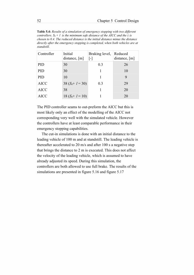
52 Chapter 5 Control Design
Table 5.4: Results of a simulation of emergency stopping with two different controllers. S0 + l is the minimum safe distance of the AICC and the λ is chosen to 0.4. The reduced distance is the initial distance minus the distance directly after the emergency stopping is completed, when both vehicles are at standstill.
Controller Initial distance, [m]
Braking level, [-]
Reduced distance, [m]
PID 30 0.3 26PID 30 1 10PID 10 1 9AICC 38 (S0+ l = 30) 0.3 29AICC 38 1 20AICC 18 (S0+ l = 10) 1 20
The PID controller seams to out-preform the AICC but this is most likely only an effect of the modelling of the AICC not corresponding very well with the simulated vehicle. However the controllers have at least comparable performance in their emergency stopping capabilities.
The cut-in simulations is done with an initial distance to the leading vehicle of 100 m and at standstill. The leading vehicle is thereafter accelerated to 20 m/s and after 100 s a negative step that brings the distance to 2 m is executed. This does not affect the velocity of the leading vehicle, which is assumed to have already adjusted its speed. During this simulation, the controllers are both allowed to use full brake. The results of the simulations are presented in figure 5.16 and figure 5.17
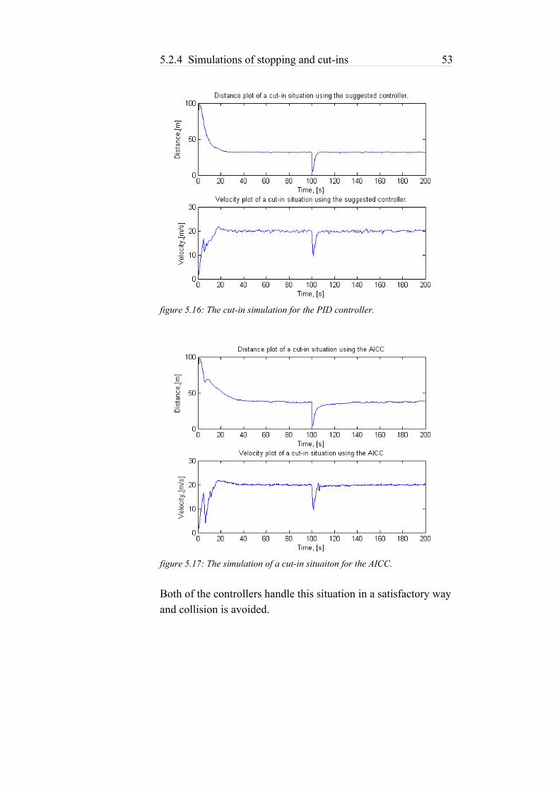
5.2.4 Simulations of stopping and cut-ins 53
figure 5.16: The cut-in simulation for the PID controller.
figure 5.17: The simulation of a cut-in situaiton for the AICC.
Both of the controllers handle this situation in a satisfactory way and collision is avoided.


Chapter 6
Implementations
ERE THE IMPLEMENTATIONS done in the different Simulink models are presented and discussed. First the
offline version of the simulator model is considered. Thereafter the changes to the online version are presented.
H
6.1 Offline simulator
THE MOST APPERENT disadvantage of the offline simulator is that there are not any other vehicles, so there is no leaders to follow. In order to do any meaningful simulations with an ACC a leader is required and must therefore be simulated. Such a simulated leader is shown in figure 6.1.
The velocity of the leader is here simulated with a signal builder block in which the velocity can be given any desirable characteristics. To the basic velocity is added a mixture of pseudo-random noise in form of both integrated noise (random-walk noise) and a simple band limited white noise.
55

56 Chapter 6 Implementations
figure 6.1: The block used for simulating the radar output when following a leading vehicle. Implemented in the offline version of the simulink model.
The input simulation shown in figure 6.1 is sufficient for simulating the single loop control approach (the normal PID controller). In the other control approaches the speed-output was also given a additative band limited white noise. The angle is not used for anything, but is still there since the radar algorithm uses it and outputs it.
In figure 6.2 the implementation of how the simulated leader from figure 6.1 connects with the controller can be seen. The distance signal is simply connected to the appropriate input (creates a negative feedback) while the speed signal is used to create the velocity difference between the leader and the simulator car. Thereafter the velocity difference signal is subtracted from the reference value, thereby creating the sought after negative feedback.
a n g l e
3
d i s t a n c e2
s p e e d
1
d i f fb a s e ve l .
S i g n a l 1
S c o p e 1
S c o p e
R a t e T r a n s i t i o n 3C o p y
R a t e T r a n s i t i o n 2C o p y
R a t e T r a n s i t i o n 1
C o p y
In t e g r a t o r 2
1s
In t e g r a t o r 1
1s
In t e g r a t o r
1s
B a n d - L i m i t e dW h i t e N o i s e 2
B a n d - L i m i t e dW h i t e N o i s e 1
B a n d - L i m i t e dW h i t e N o i s e
ve l1

6.1 Offline simulator 57
figure 6.2: The simulink model of how the simulated leader is connected with the controller and how they are connected with the throttle and brake.
In figure 6.3 the Control-block from figure 6.2 can be seen. The structure is used in both the single and double loop controllers.
figure 6.3: The simulink model of how the controller is implemented. Corresponds to the control block in figure 6.2.
B r a k e
2
A c c e l e r a t o r1
T h r e s h o l d
0 . 1
T e r m i n a t o r
S i m u l a t e d l e a d e r
v e l
s p e e d
d i s t a n c e
a n g l eS c o p e 2
R e l a t i o n a lO p e r a t o r 1
<
R e l a t i o n a lO p e r a t o r
<
P r o d u c t 1
P r o d u c t
M i n M a x 1
m a x
M i n M a x
m a x
F r o m 1V e h _ l o n g i
F r o m
V e h _ l o n g i
D e s i r e d d i s t .
3 0
C o n t r o l
R e q _ D
D i s t
A c c
B r k
A d d 1
A d d
P s _ B r k P d l
2
P s _ A P d l1
< P s _ B r k P d l >
< P s _ A P d l >
B r k2
A c c1
S c o p e 2
S c o p e 1
S a t u r a t i o n 2
S a t u r a t i o n 1
S a t u r a t i o n
P r o d u c t
P
P
N e g .
- 1
I n t e g r a t o r
1s
I
I
D - f i l t e r
D . s
D f . s + 1
A c t i v a t i o n f r o mv e h i c l e c o n t r o l
C r u i s e C o n t r o l
A b s
| u |D i s t
2
R e q _ D1

58 Chapter 6 Implementations
6.2 Online simulator
IN THE ONLINE simulator there is a few other requirements that needs to be fulfilled, as compared with the offline version. There is obviously no need for any simulated leader, as it is in the offline version, instead the input from the radar sensor in the graphics environment needs to be received and filtered. The most obvious difference to the offline version is however that the ACC must be able to pick up from the previosly existing Cruise Control as soon as a leader vehicle is found.
In figure 6.4 the implementation of the ACC is shown. The most significant changes, as compared with the previously existing Cruise Control model, are marked in gray. The controllers are switched when a leader is found or lost, see variable Leader found in figure 6.6. The blocks ACC Logics and Cruise Control Logics are basicly the same block and the only difference between the boolean signals ACCActive and CruiseControlActive is that the latter is false when the velocity is to low.
figure 6.4: An overview of the simulink model of the ACC implementation.
M o d i f i e d o n : 2 0 0 7 _ 1 2 _ 1 3B y : P ä r B e r g g r e n
A d d e d C r u i s e C o n t r o l L o g i c s . I t a l l o w s u s e o f t h e s t e e r i n g w h e e l k e y b o a r d . A C C a d d e d .
L a s t m o d i f i e d : 2 0 0 5 _ 1 0 _ 3 1B y : H e n r i k N i l s s o n & G u i l l e r m o B e n i t o
I n p u t s : A c c e l e r a t o r , b r a k e p o s i t i o n .v e h i c l e v e l o c i t y
O u t p u t : M o d i f i e d a c c e l e r a t o r a n d b r a k eD e s c r i p t i o n : C o n t r o l l s t h e v e h i c l e s p e e d t o t h e d e s i r e d v a l u e .
B r a k e2
A c c e l e r a t o r
1
m / s t o K m / h
3 . 6
T h r e s h o l d0 . 1
S w i t c h
S w i t c h
R e l a t i o n a lO p e r a t o r
<
R e l a t i o n a lO p e r a t o r
<
P r o d u c t
P r o d u c t
N O T N O T
M i n M a x
m a x
M i n M a x
m a x
L o g i c a lO p e r a t o r
A N D
L e a d e r L o g i c s
L e a d e r f o u n d
D i s t a n c e t o L e a d e r
G o t o 2 L _ f o u n d
C r u i s e C o n t r o l L o g i c s
C u r r e n t V e l o c i t y
D e s i r e d V e l o c i t y
C r u i s e C o n t r o l A c t i v e
C o n t r o l
R e q _ V
C C _ A c t i v e
V
A c c
B r kA N D
A N D
A C C L o g i c s
C u r r e n t D i s t a n c e
D e s i r e d D i s t a n c e
A C C A c t i v e
A C C C o n t r o l
R e q _ D
A C C _ A c t i v e
D
A c c
B r k
V e l o c i t y3
P s _ B r k P d l2
P s _ A P d l
1
< P s _ B r k P d l >
< P s _ A P d l >
< V _ V e h L o n g >
A c c
B r k
< A c c >
< B r k >
A c c
B r k
< A c c >
< B r k >

6.2 Online simulator 59
The reason for the regular Cruise Control to require that no leader is present, as opposed to use the ACC_Active input signal, is that the control switching should not be dependent of wether or not the cruise control or ACC is currently being used.
In figure 6.5 the contents of the block ACC logics from figure 6.4 can be seen. The block´s two outputs define the parts that make up the block: ACC Active and and Desired Distance. The state of the ACC Active signal is desided by a D-latch that only allows changes to the output if the brakes are active or if the cruise button is pressed and the brakes are not active at the same time. The D-latch updates the output with the logic complement to the brake active signal, thereby making sure that the brakes are not engaged when the ACC (same for Cruise Control) is activated.
The desired distance signal is computed as the reference value minus the velocity difference, see control approach with feedback of both velocity difference and distance on page 34. The reference value is set on the positive flank of an appropriate starting signal and can be modified by the blocks Incrementation and Decrementation of Desired Distance by pressing the plus and minus buttons on the steeringwheel.
figure 6.5: The simulink model of how the block ACC logics from figure 6.4 is implemented.
C r e a t e d o n : 2 0 0 7 _ 1 0 _ 0 1B y : P ä r B e r g g r e n
H a n d l e s a c t i v a t i o n / d e a c t i v a t i o n o f A C C a n d s e t t i n g o f
D e s i r e d D i s t a n c e u s i n g s i g n a l sa q u i r e d f r o m t h e C A N - b u s .
A C C A c t i v e
2
D e s i r e d D i s t a n c e
1
T e r m i n a t o r
S e t D e s i r e dD i s t a n c e
P l u sA N DL e a d e r _ f l a g
A N D
P e d a l B r a k eR e l a t i o n
< =
O l d D e s i r e dd i s t a n c e
N o t b r a k e sA N D
C r u i s e o n .
A N DN o t
N O T
M i n u sA N DL e a d e r _ f l a g
A N D
M e m o r y
M a x . b r a k e w . C r u i s e C o n t r o l 0 . 0 5
I n i t i a l D e s i r e d D i s t a n c e
- C -
I n c r e m e n t a t i o n o f f D e s i r e d D i s t a n c e
D e s i r e d D i s t a n c e
P l u s
C u r r e n t D i s t a n c e
D e s i r e d D i s t a n c e
H a n d B r a k e R e l a t i o n
< =
G o t o 3
D e s _ d i s t
G o t o 2
B r a k e _ a c t i v e
G o t o 1
C h a n g e _ C C _ a c t i v e
G o t o
C h a n g e _ C C _ a c t i v e _ t o
F r o m S e n s o r s
[ B r a k e _ P a d e l _ p e r c e n t a g e ]
F r o m S e n s o r s
[ H a n d _ B r a k e _ p e r c e n t a g e ]
F r o m C A N 1
S p e e d _ D i f f e r a n c e ]
F r o m C A N [ C r u i s e _ D e c r e a s e ] F r o m C A N [ C r u i s e _ I n c r e a s e ]
F r o m C A N
[ C r u i s e _ O n ]
F r o m
[ L _ f o u n d ]
D e t e c t i n c r e a s e
U > U / z
D e c r e m e n t a t i o n o f f D e s i r e d D i s t a n c e
D e s i r e d D i s t a n c e
M i n u s
C u r r e n t D i s t a n c e
D e s i r e d D i s t a n c e
D a t a T y p e C o n v e r s i o n C o n v e r t
D L a t c h
D
C
Q
! Q
B r a k e O R
a c t i v a t e C C
O R
B r a k ea c t i v e
O R
C u r r e n t D i s t a n c e
1
A c t i v a t e a n d s e t C r u i s e C o n t r o l
B r a k e s n o t a c t i v e
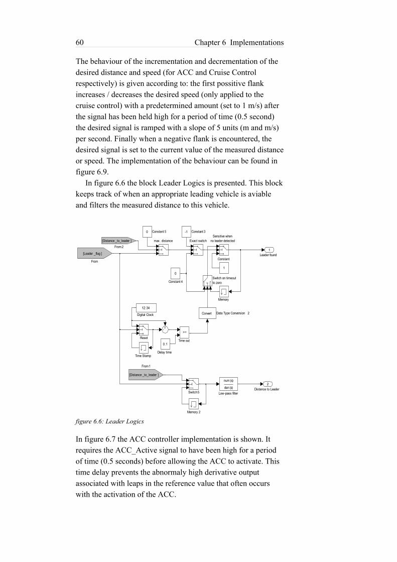
60 Chapter 6 Implementations
The behaviour of the incrementation and decrementation of the desired distance and speed (for ACC and Cruise Control respectively) is given according to: the first possitive flank increases / decreases the desired speed (only applied to the cruise control) with a predetermined amount (set to 1 m/s) after the signal has been held high for a period of time (0.5 second) the desired signal is ramped with a slope of 5 units (m and m/s) per second. Finally when a negative flank is encountered, the desired signal is set to the current value of the measured distance or speed. The implementation of the behaviour can be found in figure 6.9.
In figure 6.6 the block Leader Logics is presented. This block keeps track of when an appropriate leading vehicle is aviable and filters the measured distance to this vehicle.
figure 6.6: Leader Logics
In figure 6.7 the ACC controller implementation is shown. It requires the ACC_Active signal to have been high for a period of time (0.5 seconds) before allowing the ACC to activate. This time delay prevents the abnormaly high derivative output associated with leaps in the reference value that often occurs with the activation of the ACC.
Distance to Leader2
Leader found1
max. distance
Time out
>=
Time Stamp
Switch5
Switch on timeoutto zero
Sensitive when no leader detected
Reset
Memory 2
Memory
Low-pass filter
num (s)
den (s)
From2
[Distance _to_leader ]
From1
[Distance _to_leader ]
From
[Leader _flag ]
Exact switch
Digital Clock
12:34
Delay time
0.1
Data Type Conversion 2Convert
Constant 50
Constant 4
0
Constant 3-1
Constant
1

6.2 Online simulator 61
figure 6.7: ACC Controller
In figure 6.8 the Cruise Control Logics block found in figure 6.4 is shown.this block handles the activation of the cruise control and connects the desired velocity with the external CAN-bus controls.
figure 6.8: Cruise Control Logics
The decrementation / incrementation of desired velocity blocks that can be seen in figure 6.8 and decrementation / incrementation of desired distance in figure 6.5 are all illustrated by figure 6.9.
C r e a t e d o n : 2 0 0 7 _ 1 0 _ 0 1B y : P ä r B e r g g r e n
E x t e r n a l l o g i c s a d d e d t o a c c o m o d a t eu s e o f C C f r o m s t e e r i n g w h e e l k e y s .
L o g i c s i n b l o c k :A C C L o g i c s .
N e w i n p u t : C C _ A c t i v e
B r k2
A c c1
n e g .
- 1
T i m e s t a m p
S w i t c h
S a t u r a t i o n
S a t u r a t i o n
S a t u r a t i o n
R e l a t i o n a lO p e r a t o r
> =
P r o d u c t
P
A C C _ C o n t r o l l e r _ P
L o g i c a lO p e r a t o r
A N D
I n t e g r a t o r
1s
I
A C C _ C o n t r o l l e r _ I
H o l d t i m e
- C -
G o t o 1
C o n t r o l _ s i g n a l
G o t o
A C C _ E r r o r
D i g i t a l C l o c k
1 2 : 3 4
D e t e c tI n c r e a s e
U > U / z
D a t a T y p e C o n v e r s i o n 1C o n v e r tD a t a T y p e C o n v e r s i o n C o n v e r t D - f i l t e r
A C C _ C o n t r o l l e r _ D . s
A C C _ C o n t r o l l e r _ D f . s + 1
A b s
| u |
D3
A C C _ A c t i v e
2
R e q _ D1
e
e
u
C r e a t e d o n : 2 0 0 7 _ 1 0 _ 0 1B y : P ä r B e r g g r e n
H a n d l e s a c t i v a t i o n / d e a c t i v a t i o n o f C r u i s e C o n t r o l a n d s e t t i n g o f
D e s i r e d V e l o c i t y u s i n g s i g n a l sa q u i r e d f r o m t h e C A N - b u s .
C r u i s e C o n t r o l A c t i v e
2
D e s i r e d V e l o c i t y
1
V e l o c i t y h i g he n o u g h
< =
T e r m i n a t o r
S e t D e s i r e dV e l o c i t y
P e d a l B r a k eR e l a t i o n
< =
O l d D e s i r e dv e l o c i t y
N o t b r a k e sA N D
C r u i s e o nA N D
A b o v e M i n .v e l o c i t y
A N DN o t
N O T
M i n i m u m v e l o c i t y
- C -
M e m o r y
M a x . b r a k e w . C r u i s e C o n t r o l 0 . 0 2
L o g i c a lO p e r a t o r
N O T
I n c r e m e n t a t i o n o f f d e s i r e d v e l o c i t y
D e s i r e d v e l o c i t y
P l u s
C u r r e n t V e l o c i t y
D e s i r e d v e l o c i t y
H a n d B r a k e R e l a t i o n
< =
G o t o 3
D e s i r e d _ v e l
F r o m S e n s o r s
[ B r a k e _ P a d e l _ p e r c e n t a g e ]
F r o m S e n s o r s
[ H a n d _ B r a k e _ p e r c e n t a g e ]
F r o m C A N [ C r u i s e _ D e c r e a s e ] F r o m C A N [ C r u i s e _ I n c r e a s e ]
F r o m C A N
[ C r u i s e _ O n ]
F r o m
[ L _ f o u n d ]
D e t e c t i n c r e a s e
U > U / z
D e c r e m e n t a t i o n o f f d e s i r e d v e l o c i t y
D e s i r e d v e l o c i t y
M i n u s
C u r r e n t V e l o c i t y
D e s i r e d v e l o c i t y
D a t a T y p e C o n v e r s i o n C o n v e r t
D L a t c h
D
C
Q
! Q
C C _ I n c r e a s e A N DL e a d e r _ f l a g
A N DC C _ D e c r e a s e A N DL e a d e r _ f l a g
A N D
B r a k e O R
a c t i v a t e C C
O R
B r a k ea c t i v e
O R
C u r r e n t V e l o c i t y
1
A c t i v a t e a n d s e t C r u i s e C o n t r o l
N o t B r a k e s a c t i v e

62 Chapter 6 Implementations
figure 6.9: The block Decrementation of desired distance. All of the decrementation and incrementation blocks have this layout.
The contents of the cruise controller block, see Control in figure6.4, is shown in figure 6.10. The only difference from the previously existing block is that the integratory state has been given reseting capabilities.
figure 6.10: Cruise Controller
C r e a t e d o n : 2 0 0 7 _ 1 0 _ 0 1B y : P ä r B e r g g r e n
H a n d l e s d e c r e m e n t a t i o n o f d e s i r e d d i s t a n c e .
D e s i r e d D i s t a n c e
1
T i m e s t a m p
S e t m e m o r ys w i t c h
S e t T i m e s t a m p
S e t D e s i r e d D i s t a n c et o C u r r e n t D i s t a n c e
R e s e t v a l u e1
R e s e t m e m o r y s w i t c h
R a m p- C -
M i n u s n o t h e l dc o n s t a n t l y
0
M i n u s h e l dl o n g e r t h a n
h o l d t i m e
> =
M i n u s h a s n o tb e e n r e l e a s e d
M i n u s b e i n g h e l d A N D
h o l d t i m e h a s e l a p s e dA N D
M i n u s h a s n o t b e e n r e l e a s e d
A N D
H o l d t i m e
- C -
E n a b l e / D i s a b l er a m p
D i g i t a l C l o c k
1 2 : 3 4
D e t e c tI n c r e a s e
U > U / z
D e t e c tD e c r e a s e
U < U / z
C u r r e n tD i s t a n c e
3
M i n u s
2
D e s i r e d D i s t a n c e
1
D e s i r e d D i s t a n c e
M o d i f i e d o n : 2 0 0 7 _ 1 0 _ 0 1B y : P ä r B e r g g r e n
N e w i n p u t : C C _ A c t i v e
L a s t m o d i f i e d : 2 0 0 5 _ 1 0 _ 3 1B y : H e n r i k N i l s s o n & G u i l l e r m o B e n i t o
I n p u t s : R e q u e s t e d a n d c u r r e n t v e h i c l e v e l o c i t yO u t p u t : M o d i f i e d a c c e l e r a t o r a n d b r a k e
D e s c r i p t i o n : A P I - C o n t r o l l e r c o n t r o l l s t h e v e h i c l e s p e e d t o t h e d e s i r e d v a l u e .
B r k
2
A c c
1
S a t u r a t i o n
S a t u r a t i o n
S a t u r a t i o n
P r o d u c t
P
C C _ C o n t r o l l e r _ P
I n t e g r a t o rw . l i m i t s
1s
I
C C _ C o n t r o l l e r _ I
D a t a T y p e C o n v e r s i o n
C o n v e r t
A b s
| u |
V
3
C C _ A c t i v e
2
R e q _ V
1
ue

Chapter 7
Discussion, future work and conclusions
HIS CHAPTER STARTS with a discussion of the results and other issues related to the paper followed by a presentation
of a few ideas regarding future work. Finally some conclusions drawn from the results are brought up.
T
7.1 Discussion
THE CONTROL APPROACHES have no capabilities to handle low frequency measurement noise, which is a common problem with PID controllers. Fortunately the graphics application of the simulator produces little or no such low frequency noise, so this is not really much of a problem here. The noise that is produced by the graphics program comes from the process of discretization of the cars position as they are being propagated through the environment and this mostly contain high frequency components.
63

64 Chapter 7 Discussion, future work and conclusions
Since the CAN-bus communication program suggested uses what is known as a critical section and some implementations of those may affect the realtime clock, it is important to clarify that the type used here is a kind of synchronization primitive associated with the operating system running on the control computer. This synchronization primitive is local and only blocks the switching of threads within the process, thereby not affecting the realtime clock. It would be unfortunate If that occurred in the discussed application, since the messages sent needs to be updated within a certain time span or the heads-up display would light up with warning messages.
The model of the throttle to velocity process is designed on a step response that during most of the time desribes the highest gear. The ACC however almost never actually uses the highest gear, so if the simulation that created the step response had been formed in such a way that the top gear had not been allowed to engage, the resulting model may have described the actual process better. The only difference between gears however is that they change the gain of the closed loop system, by changing the equivalent mass of the car. Therefore the model errors introduced by higher gears should be countered by the high gain margins produced by the suggested controller.
The intuitive contol design used in selecting the parameters of the PID controller has the drawback of being suboptimal. However, the controller do take into account the stationary nonlinearities in the limitations on the control signal.
The distance plot in figure 5.14 provides information about the rise time, settling time and overthrows. The rise time seams furthermore to have an indicator in the maximum distance in the plot. The settling time is however the most relevant indicator of the controller´s quickness. The overthrows in the plot gives the first failed requirement of a controller as the PID controller with only distance feedback has several large overthrows.
The emergency stopping simulation gives information about minimum stopping distance under different maximum allowed braking levels, as can be seen in table 5.4. That the maximum braking level has such an impact on the stopping distance suggests that a separate system for emergency braking might be a good idea, as the controllers can be considered more comfortable if they cannot use full brake under normal conditions.

7.1 Discussion 65
An almost identical simulation was carried out on the AICC in (Ioannou, 1993), in which five vehicles were considdered, but no noise was added to the measurements. The results obtained in that simulation was more based on the platoon dynamics that occur when several vehicles are considdered and state that all vehicles had stopped within ten seconds and that no collision occurred. However the stopping distance can be measured in graphs and seam to be between ten and twelve meters, which cuts the ones obtained in the simulations here in half. These differences can most likely be explained with that the simulations done here are slightly more realistic (since more effort has been put into the design of the simulated vehicle) and that the AICC used is of the exact same design (in a simulated vehicle very different from what it was designed for) and the added noise.
The cut-in simulations done give additional information about the collision avoidance capabilities of the controller. However, it may be argued the simulations are done with large reference values, which produce large errors and thereby simplifies the control situations. The distance by itself however do not offer a complete view of the control situation. It needs to be viewed as a time headway in order to give relevant information about the choise of reference value. The reference value is chosen as 30 m, which at a velocity of 20 m/s gives a time headway of 1.5 seconds. The AICC was submitted to cut-in simulations under various conditions in (Ioannou, 1993) in which the results was werther collision did or did not occur. The simulations done in this paper only results in werther or not the two compared control approaches are comparable with eachother.
66 Chapter 7 Discussion, future work and conclusions
7.1.1 Future work
IMPROVE THE REALISM of the radar sensor by, for instance, creating a better criteria for the selection of a leading vehicle, so that vehicles appearing between the simulated car and the leading vehicle are detected.
Create driving situations (in the graphical environment) that tests the capabilities of the control algorithm in “real” situations. For instance, emergency stopping and cut-in situations or even more interesting, an evasive action test. This may however be a bit challanging since the development tool seams to be broken.
Implement a sensor based on image analysis. Several interesting algorithms exists, for instance using the characteristic vertical edges of cars easily identified with sobel operators or using the chromatics of the cars.
Since the system have varying gain, due to the gearbox and brakes, it may be motivated to test adaptive control strategies or gain scheduling. It may also be motivated to test any and all control algorithms more thoroughly regarding different safety situation.
Add high frequency moiton feedback to the simulator. For instance by installing electrical vibration actuators in the driving seat.
7.2 Conclusions 67
7.2 Conclusions
IN THE WORK done the best overall control performance was found when using the control approach with feedback of distance and velocity difference (see figure 5.2 on page 34 for the structure of the controller). The suggested controller is shown to eliminate persistent errors. The closed loop system (with the linear model) is stable when using the suggested controller, with good stability margins and the comfort provided is high due to the low amplitude of overthrows. It is insensitive to high frequency measurement noise and the control signal activity is limited.
The suggested changes to the CAN-bus communication program will provide the simulator with the bidirectional realtime communication necessary to provide driver interaction.
The controller is provided with feedback signals from the software based radar plug-in program suggested. However, these signals are noisy in themselves due to discretization effects in the graphics program and the numerical derivation of this effect.
The suggested control approach has safety capabilities regarding emergency stopping and cut-in situations that are deemed acceptable since no collision occurs in the considdered situations.


Bibliography
Fabian, M. (2006) Discrete Event Systems, Lecture Notes (ESS 200). Göteborg: Chalmers University of Technology. (R 004/2004) ISSN 1403-266X
Ioannou, P. A. & Chien, C. C. (1993) Autonomous Intelligent Cruise Control. IEEE TRANSACTIONS ON VEHICULAR TECHNOLOGY. p. 657 – 672. Vol. 42, No. 4, November 1993
Lennartson, B. (2002) Reglerteknikens grunder. (Fourth edition) Lund:Studentlitteratur. ISBN 91-44-02416-9
Ljung, L. and Glad, T. (2004) Modellbygge och Simulering. (Second edition) Lund: Studentlitteratur. ISBN 91-44-02443-6
Nordling, C. and Österman, J. (2004) Physics Handbook for Science and Engineering. (Seventh edition) Lund: Studentlitteratur. ISBN 91-44-03152-1
OSG Community (2007) OpenSceneGraph. http://www.openscenegraph.org (2007-11-20)
Robert Bosch GmbH. (1991) CAN Specification. (Version 2.0) Stuttgart: Bosch. www.bosch.com (2007-10-01)
Thomas, B. (2001) Modern Reglerteknik. (Third edition) Stockholm: Liber. ISBN 91-47-05085-3
Vector Informatik GmbH. CAN Driver Library for CANcardXL / CANcardX / CAN-AC2-PCI: User Interface Description. (Version 3.4) Stuttgart: Vector Informatik GmbH.

Table of figuresfigure 1.1: An overview of Chalmers Vehicle Simulator, or at least the parts that are mentioned in this paper. The lines represent different types of communications, where the CAN-bus is dashed as it is the only one considered in the paper................................................................................................................... 3figure 1.2: The top view of the Simulink model associated with the vehicle dynamics. From left to right the blocks are: all the inputs to the model (from hardware-based like throttle and steeringwheel to software-based like the wheel position generated in the graphics computer) , noise is added to represent road irregularities, the vehicle dynamics is computed in the Vehicle block, the motions of the platform is calculated in the Platform Washout block and the outgoing signals are communicated to their recipients in the Output block.............................................................................................................................................4figure 1.3: The block Vehicle from figure 1.2............................................................................................... 4figure 1.4: The vehicle control block from figure 1.3. The linear reference model is used in the ESP, which handles stability of the vehicle. The ABS block prevents the brakes from locking up. The EPS & DSR block contains both the force feedback calculation associated with the Electronic Power Steering and a steeringwheel torque associated with a Driver Steering Recommendation system implemented in a previous master thesis.................................................................................................................................... 5figure 1.5: The Cruise Control block from figure 1.4 showing the implementation of the previosly existing Cruise Control................................................................................................................................................5figure 1.6: The block named Control in figure 1.5 showing how the PI-controller is implemented.............6figure 2.1: Algorithm currently used in handling CAN-bus messages in the program CanCom.exe. The object of type framesAndSignals called fas seen in the second square in the CAN thread handles the current messages, both read from the CAN-bus and to be written to the same. The thread called “Main” displayed on the left is the programs main thread....................................................................................... 12figure 2.2: Illustration of how the reader and writer threads allocates information. The fas, a framesAndSignals object, is a database of all, or at least most, signals and their last known status...........13figure 2.3: The reader and writer from figure 2.2, modelled as Automata. It is important to know that they have separate alphabets. The “!” character means that the event is uncontrollable. ...................................14figure 2.4: The syncronization between the reader and writer found in figure 2.3. Mutual exclusion is achieved by not allowing updFAS to occur when the automaton is in the Write.Read state. .................... 15figure 3.1: A flow-chart illustrating the algorithm used to create a radar sensor plug-in to the graphics program........................................................................................................................................................ 19figure 3.2: Traffic situation illustrating how the software based radar sensor works. If one or more cars driving in your direction has its centerpoint within the dashed area, the closest one will be selected and its distance angle and velocity is returned. If no car is present within the dashed area the maximum range, the center angle (zero) and zero velocity are returned. The cake slice (dashed) has infinite height and is independent of the simulated car´s angle around y and x-axis. The illustration is done off-scale.............. 20figure 3.3: The noise of the distance signal measured with the software based radar. The reason for the periodicy of the noise comes from the source of the noise, which is the pixelation of the position of the car.................................................................................................................................................................21figure 3.4: The numerical derivation of the signal shown in figure 3.3. Illustrates the noise of the measured velocity signal..............................................................................................................................22figure 4.1: An oveview of the data stored in an iddata object containing the resulting velocity (and throttle) from a step in throttle level. Experiment carried out on the offline version of the simulink model, using the same automatic gearbox as used in the online version.................................................................24figure 4.2: The graphs used to measure the constants a and P.....................................................................26figure 4.3: Step responses of the different models designed with the data shown in figure 4.1. It is hard to tell which model is the best one from this graph, so the choise of model will be decided in the verification section.......................................................................................................................................................... 27figure 4.4: The residuals of the designed models. The closer they are to zero the better the model prediction is. The residuals are taken from the same data set as the models are design from.....................30figure 4.5: Residuals of the second order model designed with SIT, plotted together with the lines +/- 3 *

√(Pr). where Pr is given by equation (4.8). The high level of deviation for negative tau comes from that the data was collected under feedback.........................................................................................................30figure 4.6: Block diagram representation of the extension of the velocity model. Implementation done in Matlab/Simulink.......................................................................................................................................... 31figure 4.7: An illustration of how the road curvature impact the measured velocity with what is assumed to be random-walk noise. Here d is the scalar distance to the leading vehicle, y always points in the direction of the leading vehicle, vl is the vectoral speed of the leading car. .............................................. 32figure 5.1: Simulink model used for simulations of simple PID controllers. Braking simulated by taking negative part of control signal and multiplying it by ten. Limits to brake and throttle signals are set to 0.3 and 0.7 respectively in order to achieve comfort.........................................................................................34figure 5.2: Simulink model of the control loop using external feedback to make the reference value sensitive to the speed difference.................................................................................................................. 34figure 5.3: Illustration of how the proportional control parameter was selected. At an error of minus 12 meters, a control signal of minus one (full brake) is chosen. Because of the negative feedback, the error increases in the opposite direction of the vehicles. (units in meter)............................................................ 37figure 5.4: The Nyquist diagram of the circuit loop of the control loop, in a general overview................. 40figure 5.5: The Nyquist diagram in close-up around minus one..................................................................40figure 5.6: Plot of the distance response to a leading vehicle speed of 20 m/s with an initial distance of 60 m. The simulated car starts with initial speed of 0 m/s................................................................................41figure 5.7: Plot of the distance response to a leading vehicle speed of 20 m/s with an initial distance of 60 m. The simulated car starts with initial speed of 0 m/s and has a reference value of 30 m. Simulation of the Simulink model in figure 5.2................................................................................................................. 43figure 5.8: The control signal activity of the discussed controller under a simulation with a leader starting with 0 m/s and accelerating to 20 m/s (72 km/h) in 16 s and holding that velocity then on. The simulated car is first accelerated to 16.67 m/s (60 km/h) whereafter the ACC is engaged..........................................44figure 5.9: The same simulation as in figure 5.8 but without the added measurement noise. This illustrates the controllers sensitivity to measurement noise. In general the mean value of the noisy signal in figure 5.8 seams not to deviate much from the signal in this figure...................................................................... 44figure 5.10: The Bode diagram of the controller given by Table 5.2.......................................................... 45figure 5.11: Nyquist diagram of the Lu circuit loop according to equation (5.21)......................................46figure 5.12: Nyquist diagram of the Ld circuit loop, according to equation (5.23).....................................47figure 5.13: An implementation of the AICC discussed in the text. Note the derivative block necessary in the controller................................................................................................................................................ 49figure 5.14: A simulation of the different controllers.................................................................................. 50figure 5.15: The resulting control signal from a simulation with a simulated leader and carried out with the same conditions as the simulation in figure 5.8. ................................................................................... 51figure 5.16: The cut-in simulation for the PID controller............................................................................53figure 5.17: The simulation of a cut-in situaiton for the AICC................................................................... 53figure 6.1: The block used for simulating the radar output when following a leading vehicle. Implemented in the offline version of the simulink model................................................................................................56figure 6.2: The simulink model of how the simulated leader is connected with the controller and how they are connected with the throttle and brake.................................................................................................... 57figure 6.3: The simulink model of how the controller is implemented. Corresponds to the control block in figure 6.2...................................................................................................................................................... 57figure 6.4: An overview of the simulink model of the ACC implementation............................................. 58figure 6.5: The simulink model of how the block ACC logics from figure 6.4 is implemented................. 59figure 6.6: Leader Logics.............................................................................................................................60figure 6.7: ACC Controller.......................................................................................................................... 61figure 6.8: Cruise Control Logics................................................................................................................ 61figure 6.9: The block Decrementation of desired distance. All of the decrementation and incrementation blocks have this layout.................................................................................................................................62figure 6.10: Cruise Controller...................................................................................................................... 62


Appendix A: Source code for proposed CAN application changes A - I
Appendix A: Source code for proposed CAN application changesThe major changes to the CAN communication program suggested in this paper, can be found here. Most of the source code has few and outspread changes and was determined to be far to volumous to present here, therefore everything but the threads dealing with the CAN-bus communication is omitted.
void CANCom_thread(void *dummy){
//Local variables:int i = 0; //Index varable.Vstatus vErr; //Variable for status management in CAN
communication.Vevent *pEvent; //Event containing the current message.DWORD CCount = 0; //Variable for time-keeping.
threadRuning = 1;while (threadRuning) {
WaitForSingleObject(gEventHandle,10);
for (i = 1; i <= numEvents; i++) { //Update CAN-list loop.vErr = ncdReceive1(gPortHandle,&pEvent);//Deal with possible errors.if (vErr&&vErr!=VERR_QUEUE_IS_EMPTY) goto ncdError;if (vErr==VERR_QUEUE_IS_EMPTY) break;if (LogEvents)
printf("%s\n",ncdGetEventString(pEvent));
CCount = GetTickCount(); //Get time.EnterCriticalSection(&cs); //Use critical sectionFaS->canMsgframeList->CheckCan(*pEvent);
LeaveCriticalSection(&cs);} //End for-loop.
outData[0] = (char) FaS->CANUpdateReadSignals(KeyAutoStart);
FaS->CANUpdateCC(CCArray);outData[1] = CCArray[0]; //CC_OnoutData[2] = CCArray[1]; //CC_Inc.outData[3] = CCArray[2]; //CC_dec.
}// End While
DeleteCriticalSection(&cs);_endthread();
ncdError:
DeleteCriticalSection(&cs);printf("ERROR: %s\n",ncdGetErrorString(vErr));_endthread();
} // End thread.

A - II Appendix A: Source code for proposed CAN application changes
//////////////////////////////////////////////////////////////////////// CANWrite_thread()//---------------------------------------------------------------------// Thread for writing to the CAN-bus.void CANWrite_thread(void *dummy){
//Local variables:double *pFloat = (double *) &inData[4]; //Pointer for use with
communicating the global variable VehicleSpeed.int *pInt = (int *) &inData[0]; //-"- EngineRPM. DWORD CCount = 0; //Varable used for time-keeping.
threadRuning = 1;while (threadRuning) {
EngineRPM = (float) *pInt;VehicleSpeed = (float) *pFloat;
CCount = GetTickCount(); //Get time.EnterCriticalSection(&cs); //Enter critical section.FaS->CANUpdateWriteSignals(VehicleSpeed, EngineRPM);FaS->canMsgframeList->UpdateWrites(CCount, gPortHandle,
gChannelMaskLS, gChannelMaskHS);LeaveCriticalSection(&cs);Sleep(1); //Release processor from thread. Unit is in
millisec.}DeleteCriticalSection(&cs);_endthread();
} // End thread.

Appendix B:Source code for the suggested “radar” sensor B - I
Appendix B: Source code for the suggested “radar” sensor
Here source code for the so called radar sensor, developed in the context of this paper, is presented. The plug-in stucture was inspired by the existing plugins, but represents a very different use of plug-ins than the previously existing ones.
#include <stdio.h>#include <communication/TransmitterPool.h>#include <Environment/objectnodes/car.h>#include <Environment/objects.h>#include <Environment/SimCar.h>#include <osg/group>#include <Environment/world.h>#include <math.h>
extern "C"{
__declspec(dllexport) bool update(float carPos[3], Communication::TransmitterPool& transmitterPool, float output[4]){
memset(output, 0, sizeof(float)*4);//Constantsconst double l = 305; //305ft is how far this "radar" can see.const int P = 200;const int Q = 8000;const double maxAng = 90;const double PI = 3.141592685358979;const osg::Group &fwdVehicles = Environment::World::get()->getObjects()-
>getFwdDirVehicles(); //First part of all cars.const osg::Group &bwdVehicles = Environment::World::get()->getObjects()-
>getBwdDirVehicles(); //The other part of all cars.
//Global variablesdouble theta; //Angle to leader.double optTemp; //Optimization variable.double opt = 1e20; //Maximum optimization valuedouble tempL; //Temporary length.unsigned int i = 0; //For-loop iteration variable.double direction = 0; //Outgoing direction.double lOut = l; //Outgoing distance to leader. float phyCarVel = 0; //Outgoing Velocity of leader.osg::Node * node; //Temporary variable for extracting vehicles
from database.osg::Vec3 dirVec; //Vector from your car to leader.osg::Vec3 phyCarPos; //Position of vehicles in 3D.osg::Vec3 phyCarDir; //Rotation of the car's local to the global
coordinate system.osg::Vec3 carPosVec = ((Environment::ObjectNodes::PhyCar *)
Environment::SimCar::get())->getPosition(); //Your position vector.osg::Vec3 eX; //Unit vector along x-axis.osg::Vec3 eZ; //Unit vector along z-axis.osg::Vec3 planeNormal; //Normal to plane.osg::Quat carRot = ((Environment::ObjectNodes::PhyCar *)
Environment::SimCar::get())->getRotation(); //Rotation from simulated car's local to global coordinate system.
osg::Vec3 carDir; //Direction of simulated car in global coordinate system..
osg::Group * vehicles = new osg::Group; //To handle all cars.FILE * tDist = fopen("DistCase.txt","a");
Environment::ObjectNodes::PhyCar *phyCar;//Pointer to vehicle.
//Initialize variableseX.set(1,0,0);eZ.set(0,0,1);carDir.set(1,0,0);carDir = carRot*(carDir);

B - II Appendix B:Source code for the suggested “radar” sensor
//Unite vehicles in a single database.for(i = 0; i < bwdVehicles.getNumChildren(); i++) {//Put first part of all cars in Group vehicles.
node = const_cast<osg::Node *>(bwdVehicles.getChild(i));if (!vehicles->insertChild(i, node)) {
fprintf(tDist,"Error 1: error while inserting bwdVehicles.");}
}for(unsigned int ii = 0; ii < fwdVehicles.getNumChildren(); ii++) {
//Put the other part of all cars in Group vehicles.node = (osg::Node *)(fwdVehicles.getChild(ii));if (!vehicles->insertChild(i, node)) {
fprintf(tDist,"Error 2: error while inserting fwdVehicles.");}i=i+1;
}
//Search Group of all vehicles for appropriate leader car.for (i = 0; i < vehicles->getNumChildren(); i++) {
node = (osg::Node *) (vehicles->getChild(i));phyCar = (Environment::ObjectNodes::PhyCar *) (node);//Car to be examined.phyCarDir.set(1,0,0);
if (phyCar != Environment::SimCar::get()){phyCarDir = (phyCar->getRotation()) *(phyCarDir);if (carDir.operator *(phyCarDir) <= 0) { //Check if going in
opposite direction.continue;
}else {phyCarPos = phyCar->getPosition();dirVec = phyCarPos.operator -(carPosVec);//Calculate a
directional vector from simulated car to leading vehicle.
planeNormal = carDir.operator ^(eZ); //Calculate normal to plane.
theta = PI/2 - acos(dirVec.operator *(planeNormal) / (dirVec.length() * planeNormal.length())); //Calculate angle to plane.
tempL = dirVec.length(); //Distance to simulated vehicle.optTemp = P * pow(tempL-160,2) + Q * pow((abs(theta)/PI)*180,2);
//Quadratic criteria with the penalties P and Q.if (optTemp <= opt && (dirVec.operator *(carDir)) > 0) {
//Minimization of the criteria and check that leader is in front of you.
if (tempL <= l && tempL > 10) { //Check for acceptable ranges.
lOut = tempL;direction = (abs(theta)/PI)*180;phyCarVel = phyCar->getSpeedMeterPerSec();opt = optTemp;
}}
}}
}output[0] = lOut;output[1] = direction;output[2] = phyCarVel;
if (lOut >= l) {//No cars fulfill requirements. output[3] = 0;//flag, 0 = no leader found.
}else {output[3] = 1;//flag, 1 = leader found.
}
fclose(tDist);vehicles->unref();return true;
}__declspec(dllexport) const char* name(){
return "Radar Sensor";}__declspec(dllexport) const char* description(){
return "Distance, direction and velocity of the closest vehicle";}
}

Appendix C:Simulated Vehicle C - I
Appendix C: Simulated Vehicle
The Chalmers Vehicle Simulator runs a mathematical model of a Volvo XC90. The simulator has a setting that changes the engine model from a physicaly modeled simulation (basicly a Simulink model of an engine) to a 2 dimensional mapping, which outputs torque based on the engine speed (revolutions per minute) and throttle level. The mapping is presented in figure C.1.
figure C.1: Mapping of an engine´s torque output. Torque based on the engine speed and throttle level. The mapping is a possible choise in the CVS that requires less computation time than the modeled engine.
Another important component that affects preformance is the gearbox. The gearbox implemented in the simulator is of automatic type and the shifting mechanism is modelled in Simulink and as appears in figure C.2 the behavior of the mechanism introduces a complicated nonlinearity.

C - II Appendix C:Simulated Vehicle
figure C.2: The Simulink model of the automatic gear shifting mechanism. At a specific rpm rate (5000) the mechanism shifts up and at another (2300) it shifts down, unless the gearbox is in neutral.
L a s t m o d i f i e d : 2 0 0 6 _ 0 3 _ 0 9B y : H e n r i k N i l s s o n & G u i l l e r m o B e n i t o
I n p u t s : E n g i n e s p e e d [ r p m ] .O u t p u t s : g e a r [ 1 - 6 ] .
D e s c r i p c t i o n : W h e n t h e e n g i n e s p e e d i s a b o v e / b e l o w S h i f t U p R p m / S h i f t D o w n R p m t h e g e a r i n c r e a s e s / d e c r e a s e s . M e m o r y 1 i s p r e v e n t i n g a n a l g e b r a i c l o o p s .T u n a b l e P a r a m e t e r s : S h i f t U p R p m , S h i f t D o w n R p m
G e a r
1
T u r n o f f a u t o m a t i c t r a n s m i s s i o n w h e n r e v e r s i n g
0
S w i t c h 1
S w i t c h
S u m 2
S a t u r a t i o n 1
R e v e r s e g e a r
- 1
R e l a t i o n a lO p e r a t o r
~ =
P r o d u c t
N e u t r a l g e a r
T r o t t l e
W _ W h l
N e u t r a l
M e m o r y 1
M e m o r y
H i t
H i t
W _ E n g i n e _ r p m
4
W _ W h l
3
G e a r S t i c k
2
t h r o t t l e
1
G e a r