Automatic Visual Behavior Analysis - DiVA portal19307/FULLTEXT01.pdf · Automatic Visual Behavior...

Automatic Visual Behavior Analysis

Dissertation for a Master of Science Degree Applied Physics and

Electrical Engineering Control and Communication

Department of electrical engineering Linköping University, Sweden

by

Petter Larsson LiTH-ISY-EX-3259

Linköping 2002-11-11

Automatic Visual Behavior Analysis

Dissertation for a Master of Science Degree Applied Physics and

Electrical Engineering Control and Communication

Department of electrical engineering Linköping University, Sweden

by

Petter Larsson

LiTH-ISY-EX-3259 Linköping 2002-10-28

Academic advisor: Jonas Jansson

Control and Communication Linkoping Institute of Technology

Linkoping, Sweden

Examiner: Prof. Fredrik Gustavsson

Control and Communication Linkoping Institute of Technology

Linkoping, Sweden

Industrial advisor: Trent Victor

Department of Human-Systems Integration Volvo Technology Corp.

Gothenburg, Sweden

Avdelning, Institution Division, Department Institutionen för Systemteknik 581 83 LINKÖPING

Datum Date 2002-12-06

Språk Language

Rapporttyp Report category

ISBN

Svenska/Swedish X Engelska/English

Licentiatavhandling X Examensarbete

ISRN LITH-ISY-EX-3259-2002

C-uppsats D-uppsats

Serietitel och serienummer Title of series, numbering

ISSN

Övrig rapport ____

URL för elektronisk version http://www.ep.liu.se/exjobb/isy/2002/3259/

Titel Title

Automatic Visual Behavior Analysis Automatic Visual Behavior Analysis

Författare Author

Petter Larsson

Sammanfattning Abstract This work explores the possibilities of robust, noise adaptive and automatic segmentation of driver eye movements into comparable quantities as defined in the ISO 15007 and SAE J2396 standards for in-vehicle visual demand measurements. Driver eye movements have many potential applications, from the detection of driver distraction, drowsiness and mental workload, to the optimization of in-vehicle HMIs. This work focuses on SeeingMachines head and eye-tracking system SleepyHead (or FaceLAB), but is applicable to data from other similar eye-tracking systems. A robust and noise adaptive hybrid algorithm, based on two different change detection protocols and facts about eye-physiology, has been developed. The algorithm has been validated against data, video transcribed according to the ISO/SAE standards. This approach was highly successful, revealing correlations in the region of 0.999 between analysis types i.e. video transcription and the analysis developed in this work. Also, a real-time segmentation algorithm, with a unique initialization fefature, has been developed and validated based on the same approach. This work enables real-time in-vehicle systems, based on driver eye-movements, to be developed and tested in real driving conditions. Furthermore, it has augmented FaceLAB by providing a tool that can easily be used when analysis of eye movements are of interest e.g. HMI and ergonomics studies, analysis of warnings, driver workload estimation etc.

Nyckelord Keyword visual behaviour; signal processing; saccade; fixation; smooth pursuit; eye tracking; head tracking; glance analysis; glance

Abstract This work explores the possibilities of robust, noise adaptive and automatic segmentation of driver eye movements into comparable quantities as defined in the ISO 15007 and SAE J2396 standards for in-vehicle visual demand measurements. Driver eye movements have many potential applications, from the detection of driver distraction, drowsiness and mental workload, to the optimization of in-vehicle HMIs. This work focuses on SeeingMachines head and eye-tracking system SleepyHead (or FaceLAB), but is applicable to data from other similar eye-tracking systems. A robust and noise adaptive hybrid algorithm, based on two different change detection protocols and facts about eye-physiology, has been developed. The algorithm has been validated against data, video transcribed according to the ISO/SAE standards. This approach was highly successful, revealing correlations in the region of 0.999 between analysis types i.e. video transcription and the analysis developed in this work. Also, a real-time segmentation algorithm, with a unique initialization feature, has been developed and validated based on the same approach. This work enables real-time in-vehicle systems, based on driver eye-movements, to be developed and tested in real driving conditions. Furthermore, it has augmented FaceLAB by providing a tool that can easily be used when analysis of eye movements are of interest e.g. HMI and ergonomics studies, analysis of warnings, driver workload estimation etc.

Acknowledgements I would like to thank Trent Victor at Volvo Technology Corp. (VTEC), Gothenburg, Sweden for great advice and support during the project. Also a special thanks to Anders Agnvall, with whom I have discussed many ideas, and the staff at dept. 6400 for taking me in as one of their own from the very beginning. I am also grateful to SeeingMachines for developing such an extraordinary system.

Table of contents

INTRODUCTION 1

1.1 Ocular motion 3 1.1.1 Eye physiology 3 1.1.2 Ocular motion and segmentation 7

1.2 Ocular measures 8 1.2.1 Basic ocular segmentation 9 1.2.2 Glance based measures 9 1.2.3 Non-glance based measures 11

1.3 Previous work 11

1.4 Objectives of the present work 12

2 DATA COLLECTION 13

2.1 Available data 13

2.2 Technical platform 13 2.2.1 The SleepyHead (and FaceLAB) system 13 2.2.2 SleepyHead (and FaceLAB) signals 15 2.2.3 Problems associated with SleepyHead 16

3 RESULTS 18

3.1 Commonly used methods 18

3.2 Off-line algorithm architecture 20 3.2.1 Preprocessing 21 3.2.2 Basic saccade and fixation identification 23 3.2.3 Off-line information enhancement 26 3.2.4 Glance classification 26 3.2.5 Ocular measures 29

3.3 On-line (real-time) algorithm architecture 30

3.4 Off-line auto analysis compared with video transcribed data 32

3.5 On-line auto analysis compared with video transcribed data 33

4 DISCUSSION 35

5 CONCLUSIONS 37

6 FUTURE WORK 38

REFERENCES 40

APPENDIX A SLEEPYHEAD AND FACELAB SIGNALS I

APPENDIX B VALIDATION OF AUTOMATED ANALYSIS III

Automatic Visual Behaviour Analysis

1

1 Introduction There is a plethora of research on driver fatigue, distraction, workload and other driver-state related factors that creates potentially dangerous driving situations. This is not surprising considering that 96.2% of all traffic incidents are due to driver errors (Treat, 1979), where inattention is the most common primary cause (Wang et al. 1996). Numerous studies have established the relationship between eye movements and higher cognitive processes, e.g. Harbluk and Noy, (2002), Recarte and Nunes, (2000). Theses studies generally argue that eye movements reflect, to some degree, the cognitive state of the driver. In several studies, eye movements are used as a direct measure of driver attention and mental workload e.g. Harbluk and Noy, (2002), Ross, (2002). Knowing where the driver looks in real-time can prevent traffic incidents, meaning that human machine interfaces (HMIs) can be optimized and active safety functions, such as forward collision warnings, can be adapted on the basis of driver eye movements (the first one using offline analysis of many subjects, the latter using an online algorithm to adapt e.g. forward collision warning thresholds to the current driver state)

As mentioned above, analysis of eye movements is useful in the ergonomics and HMI fields. ‘Where is the best placement for an Road and Traffic Information display (RTI)?’ or ‘does this HMI pose less visual demand than another?’ These kinds of questions can be answered by analyzing subjects’ eye movements while using the device/HMI.

One major problem in the eye movement research has always been that each research team seems to use their own definitions and software to decode the eye movement signals. This makes research results difficult to compare with each other (Salvucci and Goldberg, 2000). It is desirable to have a standard that defines visual measures and conceptions. The ISO 15007 and SAE J-2396 are such standards, defining in-vehicle visual demand measurement methods and measures such as glance frequency, glance time, glance duration and the procedures to obtain them. However, the two standards focus on a video technique that relies on frame-by-frame human-rater analysis and is rather time consuming and unreliable. As the number of various in-vehicle information- and driver assistance systems increases, e.g. mobile phones, RTI and fleet systems, so will the interest for driver eye movements and other cognitive indicators. Thus, the need for a standardized, automated and robust analysis method for eye movements is imminent. There are only a handful of eye tracking systems that actually works outside the laboratory environment e.g. the El-mar Vision 2000 and ASL model 501, shown in fig 1.1, and the ASL model ETS, shown in figure 1.2.


2

Fig 1.1 Left: The El-mar Vision 2000 eye-tracker. Right: The ASL model 501 head mounted eye tracker.

The former two systems are intrusive and work less well outdoors where sunlight produces flares in mirrors and lenses. Also, the ASL model 501 only provides gaze direction with respect to the head normal. The ASL model ETS, on the other hand, is less intrusive and have better outdoors performance. It utilizes two infrared light sources with an advanced shuttering technique, which allows it to operate even during bright daylight conditions (according to ASL). This system is however not very portable.

Fig 1.2 The ASL Model ETS eye tracker


3

All three systems are vision (video) based, the only eye tracking method feasible in a vehicle due to the noisy environment e.g. fluctuating magnetic fields, vibrations and changing lightings. Other techniques include magnetic search coils (currents are induced in small coils that are attached to the cornea by a controlled magnetic field) and electro-oculography (the small voltages induced in the muscles controlling the eyes are measured via electrodes). Naturally, these techniques are not feasible in a vehicle environment. In Victor et al. (in press) a far better eye tracking system (and analysis procedure) was statistically verified to the ISO 15007 and SAE J-2396 methods. It is neither intrusive nor very environmental dependent and allows for large head movements. The system, SleepyHead (or FaceLAB), is developed by SeeingMachines in collaboration with Volvo and is based on two cameras (a stereo head) in front of the subject. Image processing software is used to compute gaze vectors and other interesting measures in real time, e.g. head position and rotation, blinking, blink frequency, eye-opening etc. Among the groundbreaking features in this software is the real-time simultaneous computation of head position/rotation and gaze rotation, which has never been done before. Also, it is not sensitive to the noisy environments in a vehicle; the primary noise component in the SleepyHead data is due to different lightings and head/gaze motion.

The intention of this work is to design and validate algorithms for automatic analysis of eye-movement data produced by the SeeingMachines head and eye-tracking system i.e. eliminate human rating as far as possible and make the analysis robust to errors and noise. This should be done according to existing ISO/SAE standards. The current work has been built on the procedures developed in ‘Automating Driver Visual Behavior Measurement’ by Victor et al. (in press).

A secondary aim is to adapt the algorithms to a real-time environment. The work is conducted at Volvo Technology Corp., Gothenburg, Sweden as a part of a larger project (VISREC) with the principal aim of investigating the possibilities of driver support based on visual behavior. Before the actual filtering and detection techniques are described however, it is important to have an understanding of basic eye movements and physical as well as signal properties of the eye tracker in use.

1.1 Ocular motion

1.1.1 Eye physiology In literature the oculumotor is described in detail; dividing ocular motion into several different categories e.g. saccades, microsaccades, smooth pursuit, vergence, tremor, drift, etc. The understanding of all different types of motion is beyond the purpose of this thesis. However, some of these conceptions are comprised in higher-level definitions. In this work, a generally accepted high-level description is adopted, dividing ocular motion into two fundamental categories: saccades and fixations. There are different opinions on how to define saccades and fixations (Carpenter (1998), Salvucci and Goldberg (2000)). The standpoint chosen here was that all data points that were not saccades should be classified as fixations (the same position as was


4

chosen by Victor et al. 2000). This includes smooth pursuits, which are found in abundance in driving, in the fixation conception (described later on).

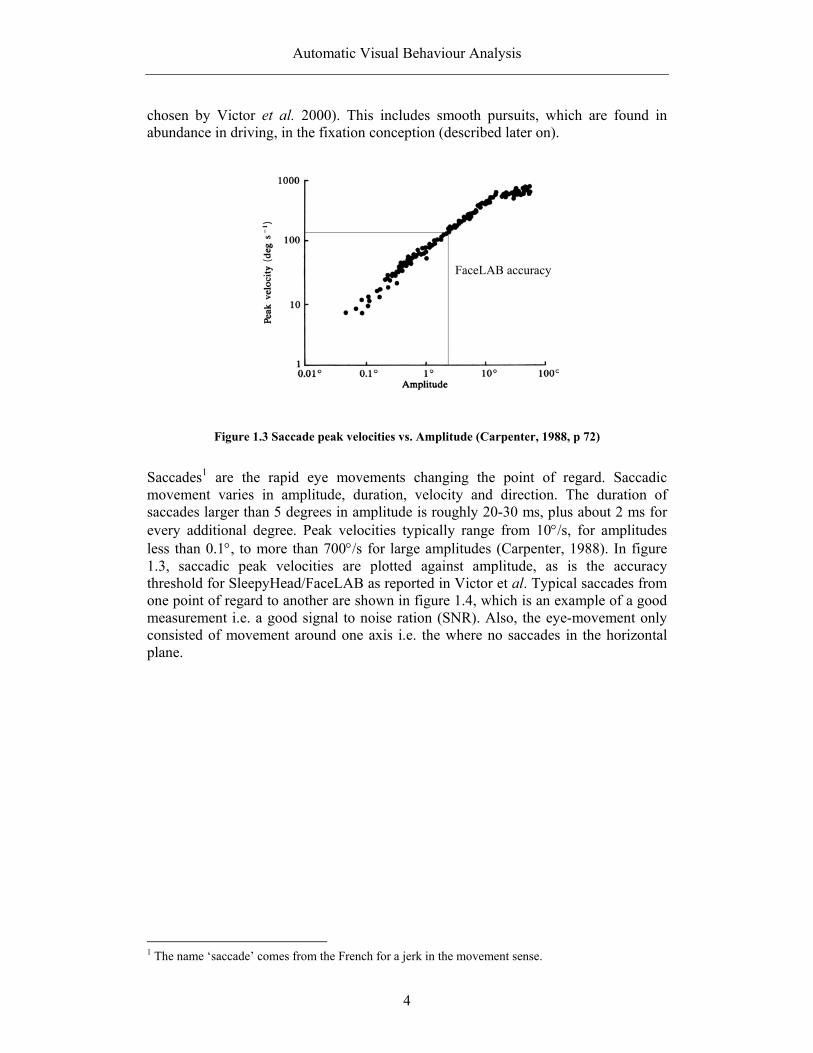
Figure 1.3 Saccade peak velocities vs. Amplitude (Carpenter, 1988, p 72)

Saccades1 are the rapid eye movements changing the point of regard. Saccadic movement varies in amplitude, duration, velocity and direction. The duration of saccades larger than 5 degrees in amplitude is roughly 20-30 ms, plus about 2 ms for every additional degree. Peak velocities typically range from 10°/s, for amplitudes less than 0.1°, to more than 700°/s for large amplitudes (Carpenter, 1988). In figure 1.3, saccadic peak velocities are plotted against amplitude, as is the accuracy threshold for SleepyHead/FaceLAB as reported in Victor et al. Typical saccades from one point of regard to another are shown in figure 1.4, which is an example of a good measurement i.e. a good signal to noise ration (SNR). Also, the eye-movement only consisted of movement around one axis i.e. the where no saccades in the horizontal plane.

1 The name ‘saccade’ comes from the French for a jerk in the movement sense.

FaceLAB accuracy


5

Fig 1.4 Gaze pitch with fixations and saccades. The two arrows mark the beginning and

termination of a saccade.

During saccadic movement our brain does not perceive information since light moves to fast over the retina2 (op cit). This absence of information forces our brains to make a calculation of amplitude and duration in advance. Inaccuracy and noise in this process almost always generates an over- or an undershot in the order of some degrees. This is corrected with drift or a new saccade, much shorter than the previous one and therefore more precise (fig 1.5). The corrective saccade is often of such low amplitude that it is undetectable to SleepyHead/FaceLAB and is considered as added noise.

Fig 1.5 Saccadic undershot, corrected with a minisaccade

2 Castet (2000) actually proved that some information is being processed during saccades. However, the subjects only had a sense they perceived a motion if an object moved at the same speed and in the same direction as the eyes. Further more, the objects where simple patterns moving over the entire visual field.


6

Figure 1.6 Drift, tremor and, at the arrow, a micro-saccade during a fixation. Both left and right

eye are shown. (Carpenter, 1988, p 125)

Fixations are defined as pauses over informative regions where the eyes can assimilate information. To be a valid fixation the pause has to last for at least 150 ms, the time our brain needs to utilize the information, Carpenter (1988). Although it is named ‘fixation’ the eyes still moves, making micro movements like drift, tremor and micro-saccades. These small movements are of very low amplitude and a part of what defines a fixation. Fig 1.6 represents a typical fixation with drift, tremor and a micro saccade. These movements are fortunately either very slow3 or very small4, which prevent their detection with the equipment used in this work.

Other larger movements, but still with sub-saccadic velocities, are called smooth pursuits. They are a subcategory of a fixation, i.e. a fixation on a moving target or a fixation on a stationary (or moving) object while the human is in motion. When we track a target, the eyes use small saccades to bring fovea on to the target and slower continuous movements at approximately the same velocity as the target. The slow movements, with velocity ranging from 80 to 160°/s, are what is referred to as smooth pursuits. This behavior is shown in figure 1.7. A subject tracks a point making a sinus curve, the signal ‘a’. The curve ‘e’ is the entire eye-movement with saccades and smooth pursuits, in ‘esa’ the pursuits are removed and in ‘esm’ the saccades are removed. (Carpenter, 1988). In general, the entire tracking behavior is referred to as a smooth pursuit and can be considered to be a drifting fixation. Hence, this behavior is from here on referred to as a fixation due to the fact that information is being processed during this movement and the saccades are two small to be detected with the system used in this work.

3 E.g. drift and microsaccades, typically in the region of 4´ s-1 and 200´ s-1 respectively. 4 E.g. tremor, typically in the region of 20´´- 40´´.


7

Figure 1.7 The eyes are tracking the pattern (a), (e) is the entire signal containing both saccade

and smooth pursuits, the saccades (esa) are removed from (esm) displaying only the tracking behavior. (Carpenter, 1988, p 55)

Apart from these three kinds of movement there is a totally different visual behavior, well worth some consideration, namely blinks. A human normally blinks about once every two seconds. This has of course a devastating impact on the gaze estimation. During the actual closure of the eyes, gaze cannot possibly be measured and since blinks do occur during both saccades and fixations it is hard to anticipate where the eyes will look when visible again. Fortunately, blinks are very fast, in the region of 250 ms for an entire blink. This means that the eyes are totally occluded for about 100-150 ms.

A very fascinating thing about blinks is that subjects are generally totally unaware of their occurrence (op cit). A more coherent and stable perception of reality is thus generated by unknowingly suppressing both saccades and blinks.

1.1.2 Ocular motion and segmentation Properties of the eyes work in favor of segmentation, meaning there are physical boundaries for ocular movements that provide rules for classification. For example: According to Carpenter (1988) (among others) one saccade cannot be followed by another with an interval less than 180 ms. Combined with the fact that it is unlikely for a saccade to last for more than 200 ms5, this implies that a saccade longer than 220 ms is more likely to be two saccades with one fixation in between. Another interesting fact is the suppression of blinks mentioned above. The subjects are generally unaware of the occurrence of blinks (op cit) and these could probably be removed (i.e. to be considered as artifacts) from the gaze signal without affecting the analysis proposed in this work. Listed below are the physical boundaries of the eyes that are relevant to this thesis: (op cit) 5 This is a consequence of saccade durations mentioned earlier. A 200 ms saccade would have an amplitude of about 90 degrees which is very uncommon. (Carpenter, 1988)


8

• A fixation lasts for at least 150 ms. • A saccade can not be followed by another with an interval less than 180 ms. • The human visual field is limited to a definable area. • A fixation can be spatially large (smooth pursuit).

• The occurrences of saccades are suppressed by the visual center. • The occurrences of blinks are suppressed by the visual center.

For the Driver of a vehicle there could be even more restrictions: • It is not likely to find fixations on the inner ceiling or on the floor during

driving, especially not during a task.

• A lot of attention (and fixations) is likely to be found on the center of road.

• Smooth pursuits velocities are low or moderate. (Oncoming traffic or road signs trigger most pursuits)

These boundaries clearly define a framework that could be used as a part of the segmentation of driver eye movements.

1.2 Ocular measures In this work measures are divided into two groups, glance based measures and non-glance based measurers. These two groups are formed by the outcome of a basic ocular segmentation where fixations, saccades and eye-closures are identified.

As mentioned before, different researchers have different methods of analyzing data and defining fixations/saccades. To have a uniform ground to stand on it is important that all data analyzing methods are based on a generally accepted international standard. This is why the measures in this work are based on the definitions in the ISO 15007-2 and SAE J-2396 standards. They both standardize definitions and metrics related to the measurement of driver visual behavior as well as procedures to guarantee proper conduction of a practical evaluation. The SAE document refers on many terms to the ISO standard and they work as a complement to each other. The equipment and procedures identified is to be used in both simulated environments as well as in road-trials. Both standards are based on a video technique, i.e. camera and VCR, with manual (off-line) classification of fixations and saccades performed by human raters. The manual video transcription is a very time consuming and potentially unreliable task. Therefore an automatic method, like the one developed in this work, is preferable. The ISO/SAE measures presented can be determined by any system classifying eye movements, either manual or automatic.

In the following three subsections the basic ocular segmentation and the two groups of measures will be described.


9

1.2.1 Basic ocular segmentation Basic ocular segmentation divides eye movements into the smallest quantities measurable with the eye-tracking system in use. These eye-movement ‘bricks’ represents a base from which all glance based and statistical measures are derived.

• Saccade – The rapid movement changing the point of regard. • Fixation (including smooth pursuit)– alignment of the eyes so that the image

of the fixated target falls on the fovea for a given time period.

• Eye closure – Short eye closures are referred to as blinks whereas long eye closures could indicate drowsiness.

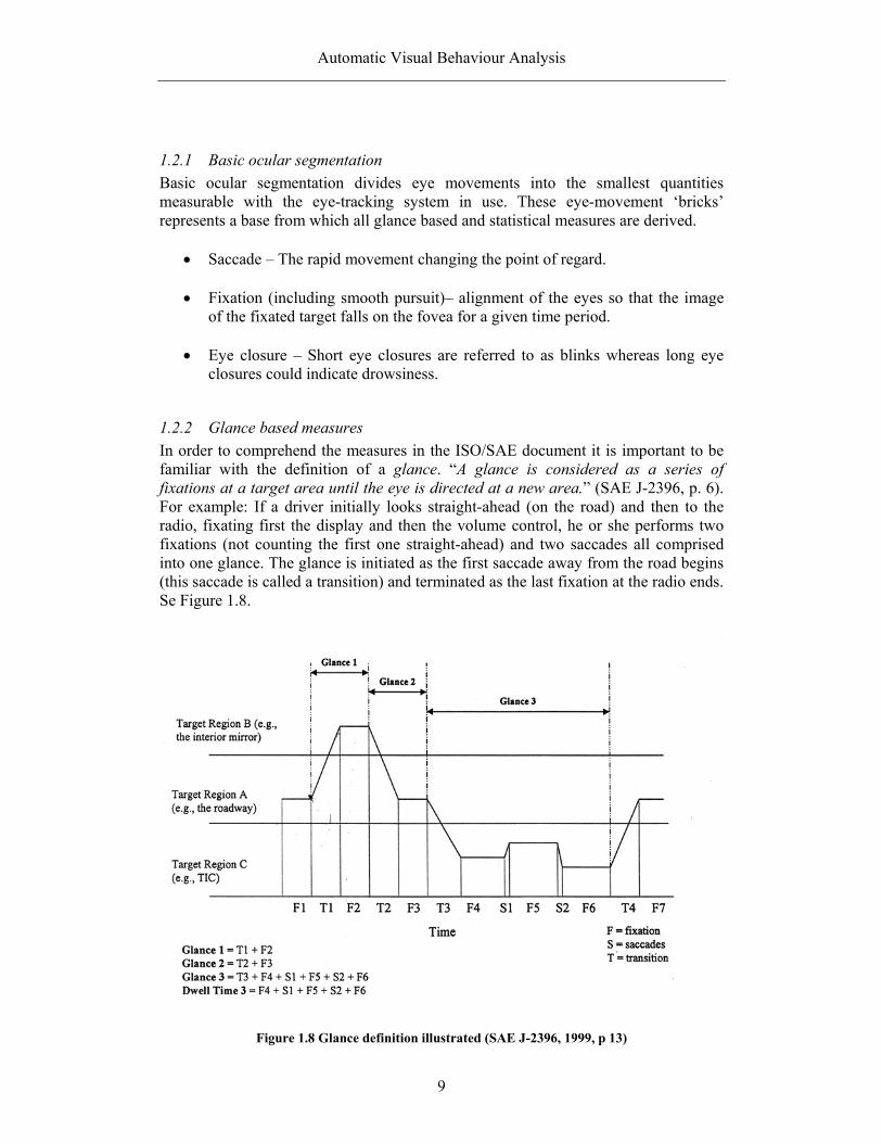
1.2.2 Glance based measures In order to comprehend the measures in the ISO/SAE document it is important to be familiar with the definition of a glance. “A glance is considered as a series of fixations at a target area until the eye is directed at a new area.” (SAE J-2396, p. 6). For example: If a driver initially looks straight-ahead (on the road) and then to the radio, fixating first the display and then the volume control, he or she performs two fixations (not counting the first one straight-ahead) and two saccades all comprised into one glance. The glance is initiated as the first saccade away from the road begins (this saccade is called a transition) and terminated as the last fixation at the radio ends. Se Figure 1.8.

Figure 1.8 Glance definition illustrated (SAE J-2396, 1999, p 13)


10

All glance-based measures are derived from this definition and are to be considered a higher-level description of eye movements formed by the ‘bricks’ described in the previous section. These measures reflect different properties such as time-sharing, workload and visual attentional demand (ISO 15007). The measures defined in the ISO and SAE document:

• Glance duration – The time from which the direction of gaze moves towards a target to the moment it moves away from it. Rather long durations are indicative of high workload demand.

• Glance frequency – The number of glances to a target within a pre-defined

sample time period, or during a pre-defined task, where each glance is separated by at least one glance to a different target. This measure should be considered together with glance duration since low glance frequency may be associated with long glance duration.

• Total glance time – The total glance time associated with a target. This

provides a measure of the visual demand posed by that location.

• Glance probability – The probability for a glance to a given location. This measure reflects the relative attentional demand associated with a target. If calculated over a set of mutually exclusive and exhaustive targets such a distribution can be used to make statistical comparisons.

• Dwell time – Total glance time minus the transition initiating the glance.

• Link value probability – The probability of a glance transition between two

different locations. This measure reflects the need to time-share attention between different target areas.

• Time off road-scene-ahead6 – The total time between two successive glances

to the road scene ahead, which are separated by glances to non-road targets.

• Transition – A change in eye fixation location from one defined target location to a different i.e. one or more saccades initiating a glance.

• Transition time – The duration between the end of a fixation on a target

location and the start of a new fixation on another target location. Since there is very little/no new information during transitions increased transition time reflect reduced availability for new driver information.

• Total task time – Total time of a task, defined as the time from the first glance

starting point to the last glance termination during the task. This definition is taken from Victor et al. (in press).

6 The “road scene ahead” excludes the rear view and side mirrors.


11

1.2.3 Non-glance based measures Non-glance based measures are all other measures that can be calculated other than those in the ISO/SAE standards, as above. Two examples are given below:

• Mean value and standard deviation of fixation position within different clusters, e.g. the road scene ahead and the phone.

• Mean value and standard deviation of fixation dwell-time within different

clusters and/or different tasks. These measures are interesting when analyzing, for example, normal driving compared to driving during high cognitive load (such as a mathematical task).

1.3 Previous work Because data reduction into glances traditionally has been very difficult and time consuming, the amount of research in the field has been limited. There are, to my knowledge, no studies where eye-tracking data, recorded in a real driving environment, has been utilized in real-time e.g. for distraction and/or risk calculation. This could be the result of time consuming manual segmentation and/or technical difficulties related to the non-portability of commonly used eye-tracking systems.

However, in studies conducted in laboratory environments a variety of algorithms have been developed. Many different approaches have been taken in segmentation algorithms using, for example, Neural Networks (Fuchuan et al., 1995), adaptive digital filters (Juhola, 1985. Wu and Bahil, 1989), Hidden Markov Models (Rabiner, 1989 and Liu, 1997), Least Mean Square methods (Gu et al., 2000. Cecchin et al., 1990), dispersion or velocity based methods (Victor. et al., (in press). Juhola M. et al. 1985. Salvucci and Goldberg, 2000) and other higher derivative methods (Wyatt, 1997). However, many of these methods specialize on the typical characteristics of its eye tracker, such as sampling frequency, and work less well with others. It should also be noted that none of the articles read prior to this work have mentioned any kind of standard when defining what and how to measure eye movements (except for Victor et al.). Furthermore, no standard refers to basic ocular segmentation (Saccades, Fixations, Eye closure), they only concern glances. Interestingly, none of the articles take smooth pursuits into account either. It seems that no one is concerned about smooth pursuits. Many studies are designed so that smooth pursuits will never occur, i.e. no objects to pursue. This is understandable; it can be difficult to differ a smooth pursuit form a saccade or a fixation. However, what strikes me is that they are hardly ever mentioned at all. Have they been neglected or are they of no relevance? Maybe they do not occur in a driving simulator as often as they do in real world driving conditions. As of now these questions remain unanswered, however smooth pursuits will be taken into account in this work because they do happen a lot in real driving conditions.


12

1.4 Objectives of the present work The general aim of the work in this thesis was to design a robust automation of the data analysis of eye movements. This should be made with focus on the measures in the ISO 15007-2 and SAE J-2396 methods for measurement of driver visual behavior with respect to transport information and control systems, especially for the Sleepyhead/FaceLAB7 eye tracking system. The analysis procedure should only require a minimum of human interaction such as loading/saving data and visual inspection of detected clusters and outliers.

Also, using the knowledge obtained during development of the off-line algorithms, a real-time algorithm was to be developed and validated. This system was to be implemented in Simulink8 and then compiled and downloaded to an industrial PC for real-time operation in a vehicle. The starting-point was the work done in “Automating driver visual behavior measurement” written by Victor et al. (in press). They showed that an automated analysis is possible using the SleepyHead system, the study revealed high correlations on all measures.

They filtered the signal using a sliding 13-sample median window filter to reduce noise, eliminate some outliers and blinks. A velocity threshold algorithm was developed to differ saccades from fixations (smooth pursuits where considered to be fixations) and a manual delimitation of clusters provided a base for glance classification. The procedure was however based on a lot of ‘know how’, the signals where filtered in Matlab and outliers, short fixations, and other artifacts were manually identified. These procedures will be eliminated.

The median filter width was not optimal for all subjects - the length needs to stand in proportion to the current noise level. Here elaboration has been done with different filter types and parameters. Also, the velocity algorithm is sensitive to noise. Hence the threshold was set to 340°/s, way above saccadic start and ending velocities. To compensate for this the two samples preceding and following a saccade was also marked to have saccadic velocities. Since saccades differ a lot in amplitude and peak velocity, so does their acceleration. Thus, this method provides only a good approximation of saccade beginnings and endings. Here the aim was to develop a more robust technique for saccade/fixation identification that also is more accurate.

Further more, a clustering technique that automatically identifies glance target areas and glances needed to be developed. It should also eliminate outliers and other artifacts. This was previously done by means of human rating. The remainder of the thesis is structured as follows. In the following chapter, the technical platform, available data and data collection are described. Chapter three describes the signal processing algorithms and the validation results, which are discussed in chapter four. The achievements and conclusions drawn from this are presented in chapter five and, finally, future work is suggested in chapter six.

7 See description in section 2.2 8 Simulink is a part of the real-time workshop in Matlab, developed by Mathworks, Camebrige.


13

2 Data collection The understanding of the origin and properties of the data used in the present work is crucial when designing detection algorithms. This chapter describes the available data and the technical platform used to obtain it.

2.1 Available data Data has been available from several studies all conducted at Volvo Technology Corp. in Gothenburg using SleepyHead/FaceLAB head pose and gaze analysis system mentioned earlier and described in the next section.

• The VDM – validation study by Victor et al. (in press) is conducted in a simulator environment at VTEC using a 7,5 m x 2,2 m ‘powerwall’ screen with 111 degrees of view and a resolution of 2456 x 750 at 48 Hz. Fourteen subjects took part in the study and various in-car tasks, such as using a mobile phone, changing radio station etc., where preformed. A more detailed description can be found in Victor et al. (in press). The data was collected with FaceLAB9 v 1.0 and is also available in video transcribed form according to the ISO 15007-2 method (ISO 1999).

• The GIB-T Vigilance study (Engström, Johansson and Victor, (forth coming)),

preformed in the VTEC driving simulator (180 degrees of view), includes 12 persons driving on a 4-lane motorway in light traffic. Each person participated on two occasions, one 30 minutes drive under normal conditions and about 2,15 hours with sleep deprivation. Recorded in Sleepyhead8 v. 3.1.1

• Currently at VTD a Volvo S80 has been equipped whit SleepyHead8 v. 3.1.1

and a video recorder. This set is part of a larger on-road experiment where 16 subjects participate. Each person performs various in-car tasks during a 30 km drive and about 15 minutes of normal motorway driving.

2.2 Technical platform

2.2.1 The SleepyHead (and FaceLAB) system SleepyHead, which is a further development of FaceLAB (as described in Victor et al. (in press)), is a head pose, gaze and eyelid closure analysis system developed exclusively for Volvo. This system tracks the head position and angle as well as the gaze angle with respect to a fixed coordinate system. It has been developed by Seeingmachines, a spin-off company from Australian National University, and Volvo Technology Corp. SleepyHead uses stereo-vision, i.e. two cameras in front of the subject (placed in front of the instrument clusters behind the steering wheel in the current prototype, se figure 2.1), to track head position and gaze. This is a considerable improvement to other existing eye tracking systems that almost always


14

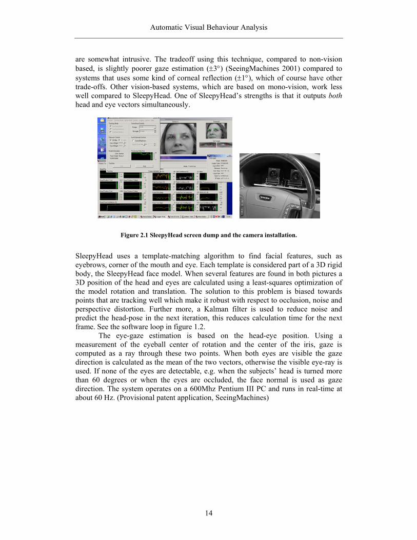
are somewhat intrusive. The tradeoff using this technique, compared to non-vision based, is slightly poorer gaze estimation (±3°) (SeeingMachines 2001) compared to systems that uses some kind of corneal reflection (±1°), which of course have other trade-offs. Other vision-based systems, which are based on mono-vision, work less well compared to SleepyHead. One of SleepyHead’s strengths is that it outputs both head and eye vectors simultaneously.

Figure 2.1 SleepyHead screen dump and the camera installation.

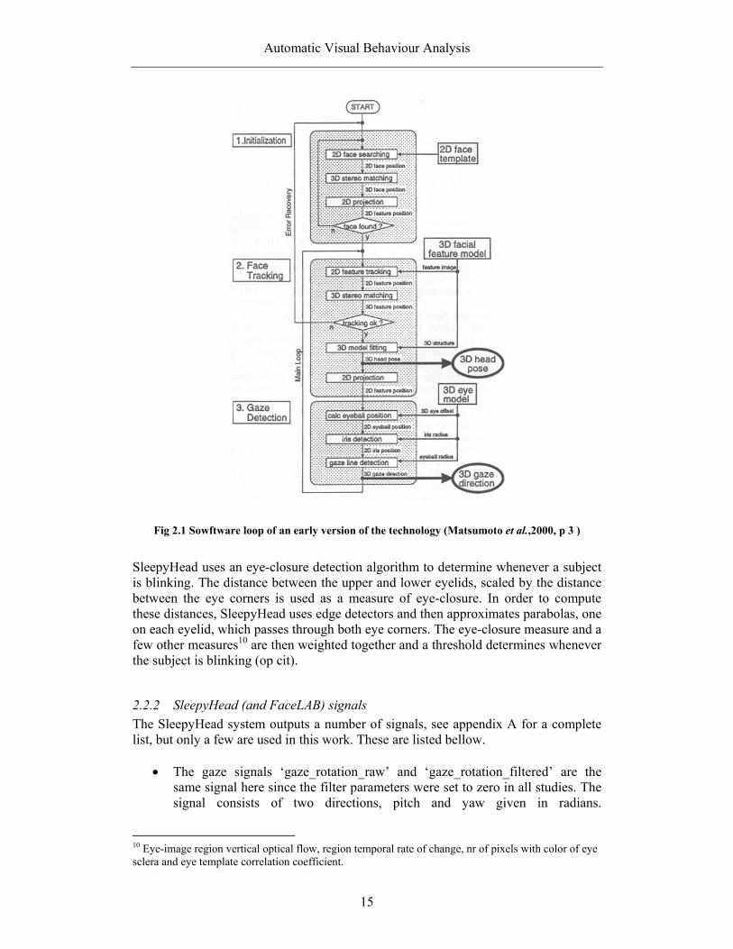
SleepyHead uses a template-matching algorithm to find facial features, such as eyebrows, corner of the mouth and eye. Each template is considered part of a 3D rigid body, the SleepyHead face model. When several features are found in both pictures a 3D position of the head and eyes are calculated using a least-squares optimization of the model rotation and translation. The solution to this problem is biased towards points that are tracking well which make it robust with respect to occlusion, noise and perspective distortion. Further more, a Kalman filter is used to reduce noise and predict the head-pose in the next iteration, this reduces calculation time for the next frame. See the software loop in figure 1.2.

The eye-gaze estimation is based on the head-eye position. Using a measurement of the eyeball center of rotation and the center of the iris, gaze is computed as a ray through these two points. When both eyes are visible the gaze direction is calculated as the mean of the two vectors, otherwise the visible eye-ray is used. If none of the eyes are detectable, e.g. when the subjects’ head is turned more than 60 degrees or when the eyes are occluded, the face normal is used as gaze direction. The system operates on a 600Mhz Pentium III PC and runs in real-time at about 60 Hz. (Provisional patent application, SeeingMachines)


15

Fig 2.1 Sowftware loop of an early version of the technology (Matsumoto et al.,2000, p 3 )

SleepyHead uses an eye-closure detection algorithm to determine whenever a subject is blinking. The distance between the upper and lower eyelids, scaled by the distance between the eye corners is used as a measure of eye-closure. In order to compute these distances, SleepyHead uses edge detectors and then approximates parabolas, one on each eyelid, which passes through both eye corners. The eye-closure measure and a few other measures10 are then weighted together and a threshold determines whenever the subject is blinking (op cit).

2.2.2 SleepyHead (and FaceLAB) signals The SleepyHead system outputs a number of signals, see appendix A for a complete list, but only a few are used in this work. These are listed bellow.

• The gaze signals ‘gaze_rotation_raw’ and ‘gaze_rotation_filtered’ are the same signal here since the filter parameters were set to zero in all studies. The signal consists of two directions, pitch and yaw given in radians.

10 Eye-image region vertical optical flow, region temporal rate of change, nr of pixels with color of eye sclera and eye template correlation coefficient.


16

‘Gaze_rotation_raw’ is only available in FaceLAB. However, with all filter settings set to zero in SleepyHead the filtered signal stays ‘raw’.

• The ‘gaze_confidence’ signal provides a confidence measure for the gaze

estimation algorithm. • ‘Head_position_filtered’ and ‘head_rotation_filtered’ uniquely determines the

3D position and rotation of the head. These are the same as ‘head_position_raw’ and head_rotation_raw’ since all filter parameters where set to zero in the available data. The ‘raw’ signals are only available in FaceLab.

• ‘Tracking’ indicates if the system is in tracking or search mode.

• ‘Blinking’ indicates if the subject is blinking.

• ‘Time’ is the cpu time associated with each estimation.

2.2.3 Problems associated with SleepyHead v1.1 It would seem that the information content in the gaze signal is not at all constant but rather varying over time. During recordings there are occasional glances towards objects that are unlikely to be focused at this point e.g. subject’s knees, inner ceiling of the vehicle etc. Some of these glances can be referred to as undetected eye-closures, which causes a dip in the gaze signal, but far from all. Another dilemma is the sensitivity to different lightings. SleepyHead is capable of handling changes in background lighting, however not when the change is rapid e.g. when a vehicle moves out from a shadowy road strip into a sunny. The result is a high noise level and sometimes almost non-existent information content. Direct sunlight into the camera lenses makes the signal even noisier due to lens flares. Occasionally this leads to the loss of tracking for several seconds.

The ‘dip’ mentioned above during eye-closures is doubtless due to the fact that the eyes are closing which leads to an approximation failure (as mentioned in the introduction). The dip is very obvious in the pitch signal, 30 – 40 degrees, but can also be perceived in the yaw signal. A typical blink lasts in the order of 250 ms (Carpenter 1988) but the dip however, last only for about 100 ms. Thus, the estimation does not collapse until the eyes are almost shut. The dips are easily removed in the preprocessing stage using a median filter. However in the SleepyHead11 system that was used to collect some of the data, an attempt to remove eye-closures from the gaze signal is done by SeeingMachines. The solution chosen is not optimal. It simply cuts out the blinking part indicated by the blink signal (which also presents a problem, discussed later) and linearly interpolates between the last known sample and the first new one, se fig 2.2. The result is big chunks of data, often almost 300 ms, which is removed and replaced with something rather unnatural – a straight line. Since blinks often occur during saccades no proper measurements can be done. Obviously this data somehow needs to be reconstructed in order to make accurate measurements.

11 SleepyHead version 3.1.1


17

As mentioned above the blink signal is a problem as well, it is not (in my opinion) always consistent with reality. This is obvious when the subject performs tasks and, according to the blink signal, virtually do not blink at all whereas in reality he/she does. It seems that the more subjects move their head, the less accurate is the blink signal.

Fig 2.2 SleepyHead gaze horizontal signal with interpolated blinks.

The gaze confidence signal would probably be a nice way to get around a lot of the problems mentioned above. However in my experience the signal quality and gaze confidence measure does not always seem to correlate. It seems to differ a lot, not only for different subjects but also for different runs using the same subject. Further more, the confidence measure drops to zero with every blink, this is expected but makes it difficult to use. Consider an undetected blink, there is no way to be certain that it was a blink that drove confidence to zero or an artifact. Hence, the confidence signal is only used as an indication in this work.

The computation rate of “about 60 Hz” mentioned earlier presents another kind of problem; the sampling interval is not constant but rather dependent of the computation time for each frame. In FaceLAB 1.0 there was no way to compensate for these differences due to low precision in the time signal. In SleepyHead however, time is available both in seconds and milliseconds as well as a computation delay-signal in milliseconds. The delay is in the region of 150-200 ms.

Finally, different subjects have different facial features making them more or less suitable for SleepyHead/FaceLAB measurements. Facial features with good contrast often correlate with good data quality, so does correct head position i.e. centered in the camera view.


18

3 Results The design of change detection algorithms is always a compromise between detecting true changes and avoiding false alarms. Varying noise and signal properties makes the gray zone even larger. Since the signal quality varies the idea was to use an adaptive filter to come around this problem. Generally when an adaptive filter is proposed, the filtering coefficient adapt to the signal using some kind of estimation process e.g. Least Mean Square (LMS). However, the FaceLAB/SleepyHead signals proved to have characteristics, such as changing information content and strange artifacts, which makes them less suitable for this kind of adaptation. Instead, a hybrid algorithm that makes use of two pre-processing median filters was developed. This is described in this chapter both for an off-line and a real-time algorithm. But first a brief review of some different algorithms commonly used for eye movement segmentation.

3.1 Commonly used detection methods In “Identifying Fixations and Saccades in Eye-Tracking Protocols” Salvucci and Goldberg (2000) have gathered several different techniques for identifying saccades and fixations.

• Velocity-based o Velocity-Threshold Identification (VT-I) o Hidden Markov Model Identification (HMM-I)

• Dispersion-based o Dispersion-Threshold Identification (DT-I) o Minimized Spanning Tree (MST) Identification (MST-I)

• Area-based o Area-of-Interest Identification (AOI-I)

Three of these where considered to be of interest for the conditions and purpose of this work: VT-I, HMM-I and DT-I. The main problem with AOI-I and MST-I are that they do not apply to the ISO/SAE standards as easily as the others. For a more detailed description see Salvucci and Goldberg (2000).

Since verified work had already been done on the VT-I method (Victor. et al., in press) a first approach was done using the DT-I method, se pseudocode in fig 3.1.


19

Fig 3.1 Pseudocode for the DT-I algorithm

According to the article the DT-I algorithm is very accurate and robust, however the inaccuracy and noise of the eye tracker used here makes it less suitable. Saccades are identified due to noise and spikes, and fixations beginnings/endings are inaccurate due to SleepyHead/FaceLAB signal properties e.g. occasional drift before a fixation becomes stationary (more or less anyway). Another problem is smooth pursuits, which causes the algorithm to collapse due the convention in section 1.1; it states that a smooth pursuit is to be considered as one fixation. Thus, the dispersion method cannot be used alone.

Fig 3.2 Pseudocode for the HMM-I algorithm

The HMM-I, on the other hand, makes use of probabilistic analysis to determine the most likely identification, se pseudocode in Fig 3.2. The HMM model in HMM-I is a two state model. The first state represents higher velocity saccade points; the second state represents lower velocity fixation points. Given its transition probabilities the HMM-I determines the most likely identification of each protocol point by means of maximizing probabilities. The algorithm is considered to be very accurate and robust given the right parameters. These are estimated using a re-estimation process, the

While there still are points Initiate window over first points to cover the duration threshold

If dispersion of window points <= threshold

Add additional points to the window until dispersion > threshold

Note a fixation at the centroid of the window points

Remove window points from points

Else

Remove first point from points Return fixations

Calculate point-to-point velocities for each point in the protocol Decode velocities with two-state HMM to identify points as fixation or saccade points Collapse consecutive fixation points into fixation groups, removing saccade points Map each fixation group to a fixation at the centroid of its points Return fixations


20

primary intricacy of HMMs. The implementation of this estimation is both complex and tedious. In the case of SleepyHead/FaceLAB, drifting signal properties makes it even more complex. Also, the data sets that are to be analyzed in the off-line processing are too small for a proper re-estimation process.

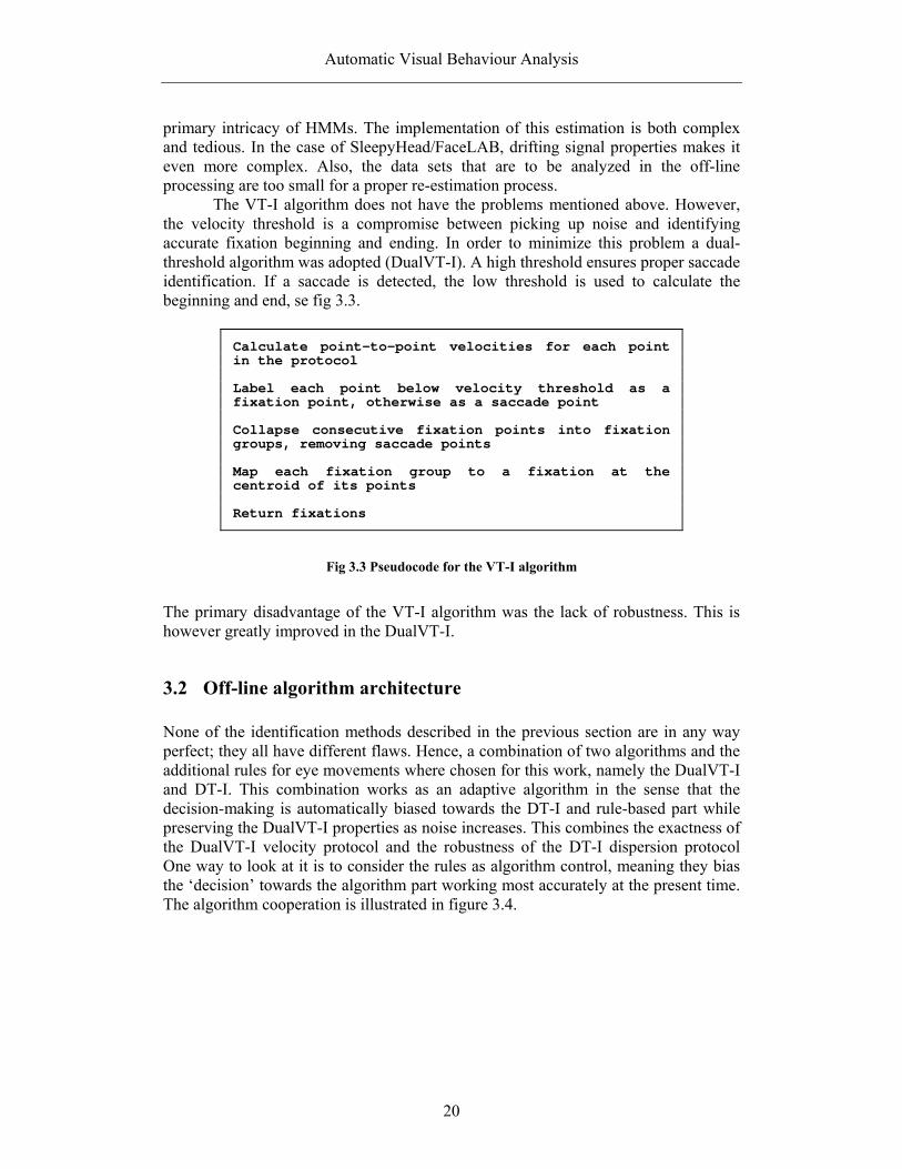
The VT-I algorithm does not have the problems mentioned above. However, the velocity threshold is a compromise between picking up noise and identifying accurate fixation beginning and ending. In order to minimize this problem a dual-threshold algorithm was adopted (DualVT-I). A high threshold ensures proper saccade identification. If a saccade is detected, the low threshold is used to calculate the beginning and end, se fig 3.3.

Fig 3.3 Pseudocode for the VT-I algorithm

The primary disadvantage of the VT-I algorithm was the lack of robustness. This is however greatly improved in the DualVT-I.

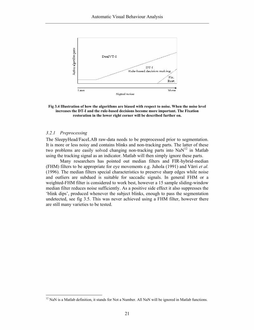
3.2 Off-line algorithm architecture None of the identification methods described in the previous section are in any way perfect; they all have different flaws. Hence, a combination of two algorithms and the additional rules for eye movements where chosen for this work, namely the DualVT-I and DT-I. This combination works as an adaptive algorithm in the sense that the decision-making is automatically biased towards the DT-I and rule-based part while preserving the DualVT-I properties as noise increases. This combines the exactness of the DualVT-I velocity protocol and the robustness of the DT-I dispersion protocol One way to look at it is to consider the rules as algorithm control, meaning they bias the ‘decision’ towards the algorithm part working most accurately at the present time. The algorithm cooperation is illustrated in figure 3.4.

Calculate point-to-point velocities for each point in the protocol Label each point below velocity threshold as a fixation point, otherwise as a saccade point Collapse consecutive fixation points into fixation groups, removing saccade points Map each fixation group to a fixation at the centroid of its points Return fixations


21

Fig 3.4 Illustration of how the algorithms are biased with respect to noise. When the noise level

increases the DT-I and the rule-based decisions become more important. The Fixation restoration in the lower right corner will be described further on.

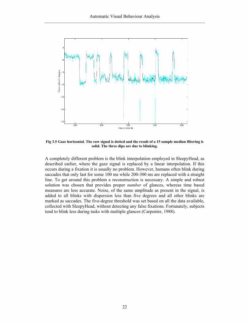
3.2.1 Preprocessing The SleepyHead/FaceLAB raw-data needs to be preprocessed prior to segmentation. It is more or less noisy and contains blinks and non-tracking parts. The latter of these two problems are easily solved changing non-tracking parts into NaN12 in Matlab using the tracking signal as an indicator. Matlab will then simply ignore these parts. Many researchers has pointed out median filters and FIR-hybrid-median (FHM) filters to be appropriate for eye movements e.g. Juhola (1991) and Värri et al. (1996). The median filters special characteristics to preserve sharp edges while noise and outliers are subdued is suitable for saccadic signals. In general FHM or a weighted-FHM filter is considered to work best, however a 15 sample sliding-window median filter reduces noise sufficiently. As a positive side effect it also suppresses the ‘blink dips’, produced whenever the subject blinks, enough to pass the segmentation undetected, see fig 3.5. This was never achieved using a FHM filter, however there are still many varieties to be tested.

12 NaN is a Matlab definition, it stands for Not a Number. All NaN will be ignored in Matlab functions.


22

Fig 3.5 Gaze horizontal. The raw signal is dotted and the result of a 15 sample median filtering is

solid. The three dips are due to blinking.

A completely different problem is the blink interpolation employed in SleepyHead, as described earlier, where the gaze signal is replaced by a linear interpolation. If this occurs during a fixation it is usually no problem. However, humans often blink during saccades that only last for some 100 ms while 200-300 ms are replaced with a straight line. To get around this problem a reconstruction is necessary. A simple and robust solution was chosen that provides proper number of glances, whereas time based measures are less accurate. Noise, of the same amplitude as present in the signal, is added to all blinks with dispersion less than five degrees and all other blinks are marked as saccades. The five-degree threshold was set based on all the data available, collected with SleepyHead, without detecting any false fixations. Fortunately, subjects tend to blink less during tasks with multiple glances (Carpenter, 1988).


23

3.2.2 Basic saccade and fixation identification

Fig 3.6 The off-line algorithm

As mentioned earlier, the identification algorithm chosen is a hybrid between the velocity and dispersion protocol as well as rules outlined by the physical properties of the eyes and eye tracker equipment. The processes run in series, at first the velocity protocol using a dual threshold is applied and then the dispersion protocol with the physical rules (as described in section 1). This is illustrated in fig 3.6. A fixation restoration algorithm is used when noise or some other property of the signal has prevented the detection of a fixation (that should be there according to the ocular rules). This is illustrated as an arrow back from the DT-I and rule-based block to the DualVT-I block. Also, the automatic clustering algorithm has been included into the hybrid shell since it administers the glance detection. Each algorithm part will now be further described. The derivative (velocity) estimate is computed by means of a two-point central difference,

hhyhyy

2)()()( −−+

=∂xxx (3.1),

applied to each gaze component and then weighted together with a square-sum-root,

22pitchyaw yyv ∂+∂= (3.2),


24

to form the 2-D velocity. Noise is always a problem when differentiating a signal, one way to handle this problem is to low-pass filter the derivatives. The central difference however, can be described as an ideal differentiator and a low-pass filter in series. The frequency response is calculated as shown in equation 3.3.

TTjTYTY )sin()()( ωωω =& (3.3)

With the sampling rate set to approximately 60 Hz, this filter has a 3 dB cut off frequency of about 14 Hz. This rather low cut-off prevents aliasing, ensuring that frequencies of more than 30 Hz are subdued but still high enough not to distort saccade beginnings and endings. The dual thresholds and the velocity estimate are shown in figure 3.7.

Fig 3.7 Solid: Eye motion velocity with the two thresholds. Dotted: Gaze horizontal. It should be noted that the eye velocity is computed from both gaze signals. In this example the vertical gaze

component had very small velocities and is therefore left out of.

One experimental comparison of five derivative algorithms found the two-point central difference to be the most accurate technique for 12-bit data (Marble et al. 1981). Among the advantages of this method are that it is simple, accurate and fast. Thresholds for the saccade detection where set primarily by comparing the results with the analysis done in ‘Automating Visual Behavior Measurement’ (Victor et. al., in press). Now, although the derivative approximation is automatically low-pass filtered it is still very noisy, the noise level being at approximately 70 °/s. However, since the SleepyHead system has an inaccuracy of ± 3° at the best (SeeingMachines, 2001) and according to Carpenter (1988) the peak velocity of saccadic movement is higher than


25

100°/s for amplitudes larger than three-four degrees (se fig 1.3) this impose no problem. Practical evaluations, however, have shown that the occasional error may slip through, especially when noise increases. Those inaccurate identifications are detected and removed by the DT-I part in the next step of the segmentation process. Thus the accuracy tradeoff using three samples for the velocity estimation has proved to be negligible.

Fig 3.8 Segmented gaze signal. Fixations are marked with thick points.

In the second step the physical criteria’s stated in chapter 1 and parts of the dispersion-based algorithm determine if detected saccades and fixation are valid. When the noise level is high the derivative approximation becomes more sensitive and confusing artifacts are occasionally detected within fixations. Their removal has a few ground rules preventing misjudgment:

1. A saccade can be altered into part of a fixation if the new fixation dispersion is less than a threshold13.

2. A saccade can be altered into part of a fixation if the variance of the fixations

is less than a threshold14. If these criteria’s are fulfilled the two fixations are joined using a linear interpolation with some added noise. The noise is introduced in order not to make this part of the signal non-physical. The original signal often contains a spike of some sort, hence the interpolation.

13 The threshold is user defined and currently set to about 7 degrees by trial and error. 14 This threshold has been set by trial and error.


26

Likewise, fixations are removed and simply marked as saccades if they are non-physical, meaning the duration is less than some 150 ms. This occurs when the signal’s information content is low.

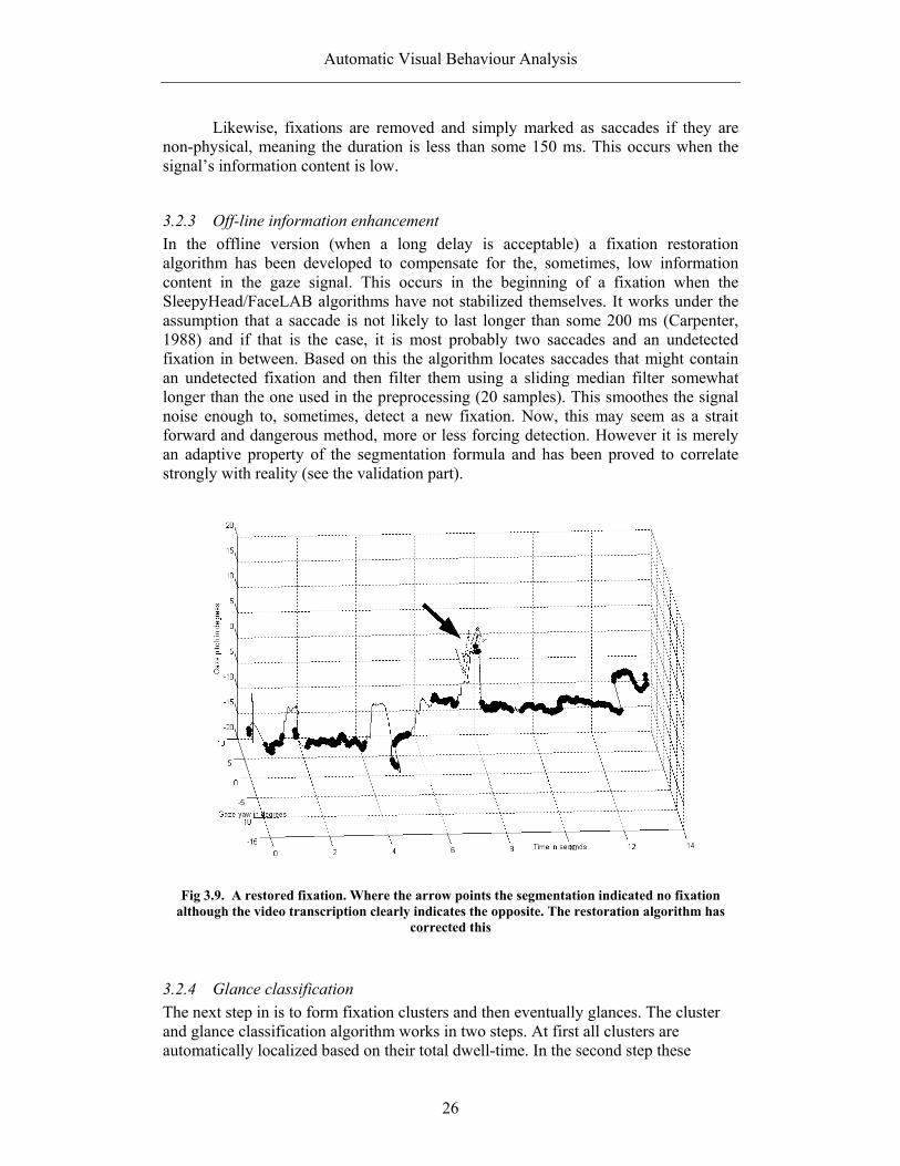
3.2.3 Off-line information enhancement In the offline version (when a long delay is acceptable) a fixation restoration algorithm has been developed to compensate for the, sometimes, low information content in the gaze signal. This occurs in the beginning of a fixation when the SleepyHead/FaceLAB algorithms have not stabilized themselves. It works under the assumption that a saccade is not likely to last longer than some 200 ms (Carpenter, 1988) and if that is the case, it is most probably two saccades and an undetected fixation in between. Based on this the algorithm locates saccades that might contain an undetected fixation and then filter them using a sliding median filter somewhat longer than the one used in the preprocessing (20 samples). This smoothes the signal noise enough to, sometimes, detect a new fixation. Now, this may seem as a strait forward and dangerous method, more or less forcing detection. However it is merely an adaptive property of the segmentation formula and has been proved to correlate strongly with reality (see the validation part).

Fig 3.9. A restored fixation. Where the arrow points the segmentation indicated no fixation

although the video transcription clearly indicates the opposite. The restoration algorithm has corrected this

3.2.4 Glance classification The next step in is to form fixation clusters and then eventually glances. The cluster and glance classification algorithm works in two steps. At first all clusters are automatically localized based on their total dwell-time. In the second step these


27

clusters are clustered themselves, based on the same dwell data, and world model objects are formed. A world model is a simple description of different pre-defined view areas e.g. the right rear view mirror or the road straight ahead. All models are defined in a plane perpendicular to the driver when he/she looks at the road straight ahead (se fig 3.12).

Fig 3.10 Multiple glances from the road-ahead-scene to the radio.

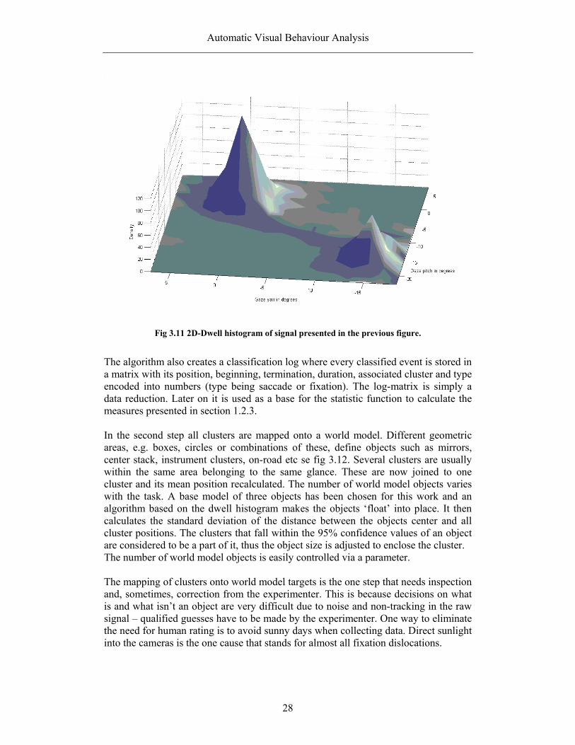
In the first step a rough approximation of cluster locations is done using a 2D dwell-time-histogram i.e. total fixation time in different view areas based on the duration and mean position of each fixation. See fig 3.10 and 3.11. Usage of the mean position has proved to be a simple way to reduce noise problems. The histogram bin-size was set to 3-by-3 degrees, mainly by trial an error. This creates a nice, smooth histogram where every peak indicates the approximate position of a cluster. Since gaze data is given in radians the actual cluster plane is not a plane but rather the inside of a sphere, thus the gaze angle does not affect the cluster size. Once the approximate cluster positions are determined every mean fixation-point is assigned to the nearest cluster-point, by Euclidian means. All clusters are then updated to the mean position of the points associated to respective cluster.


28

Fig 3.11 2D-Dwell histogram of signal presented in the previous figure.

The algorithm also creates a classification log where every classified event is stored in a matrix with its position, beginning, termination, duration, associated cluster and type encoded into numbers (type being saccade or fixation). The log-matrix is simply a data reduction. Later on it is used as a base for the statistic function to calculate the measures presented in section 1.2.3. In the second step all clusters are mapped onto a world model. Different geometric areas, e.g. boxes, circles or combinations of these, define objects such as mirrors, center stack, instrument clusters, on-road etc se fig 3.12. Several clusters are usually within the same area belonging to the same glance. These are now joined to one cluster and its mean position recalculated. The number of world model objects varies with the task. A base model of three objects has been chosen for this work and an algorithm based on the dwell histogram makes the objects ‘float’ into place. It then calculates the standard deviation of the distance between the objects center and all cluster positions. The clusters that fall within the 95% confidence values of an object are considered to be a part of it, thus the object size is adjusted to enclose the cluster. The number of world model objects is easily controlled via a parameter.

The mapping of clusters onto world model targets is the one step that needs inspection and, sometimes, correction from the experimenter. This is because decisions on what is and what isn’t an object are very difficult due to noise and non-tracking in the raw signal – qualified guesses have to be made by the experimenter. One way to eliminate the need for human rating is to avoid sunny days when collecting data. Direct sunlight into the cameras is the one cause that stands for almost all fixation dislocations.


29

The world model approach could be very useful for other measurement purposes besides glance classification e.g. on-road off-road ratio and larger scale visual scan-patterns. It is also useful when the gaze signal is noisy or corrupt (e.g. by sunlight) and fixations are scattered in larger areas forming more clusters than there really are. During the process the log-matrix is updated continuously.

Fig 3.12 The mapping of gaze onto in vehicle objects

FaceLAB produces an object classification of its own in real-time. There are two problems with this:

1. It needs to be calibrated for each and every subject and run. 2. The objects often need to be defined larger than they really are due to the

FaceLAB inaccuracy. It is difficult to determine how large a world object needs to be before examining the data. If the object is too large there is always a possibility that outliers are included or that objects has to overlap each other. The world model adjustment can also be done in the FaT-toolbox, available on the SeeingMachines website.

In the light of this it is easier to define the world model when analyzing the data and let it adapt to the current situation.

3.2.5 Ocular measures At last, the ocular measures are produced using the log-matrix constructed earlier. The measures are as defined in chapter 1:

• Dwell time • Glance duration • Glance frequency • Total glance time • Glance probability • Link value probability • Time off road scene ahead • Total task time


30

• Transition time Once the glance classification is done the calculation of these measures are very straightforward and will therefore be left out.

3.3 On-line (real time) algorithm architecture

Fig 3.13 The on-line (real-time) algorithm

The real time implementation is a first prototype and works very much like the off line algorithm. The differences are that only ‘road-scene-ahead’ and ‘other-areas’ are defined as world model objects. The output is, for each task, total number of glances and total glance-time on and off road. Task beginning and ending are indicated in the SleepyHead/FaceLAB log-file by annotations or time-gaps (this is done manually during logging). Before any classification is done the road-scene-ahead world object is localized. This is done using an initialization phase, calibrating the setup for the particular subject and run. The road-scene-ahead area is localized by means of a gaze density function. Most of the driver attention is directed in this area and the dwell time density function always have a very significant peak in the center of it (as can be seen in fig 3.11). The distribution of fixations in this area is approximated to be gaussian. Thus, the standard deviation can be computed using the highest point in the dwell histogram as the average fixation position value. Technically it is not the standard deviation being calculated, but rather deviation of mode. The road-scene-ahead is then considered to be within the 95% confidence values. The procedure is done for both yaw and pitch


31

directions respectively, thus forming an oval area that represents the road-scene-ahead.

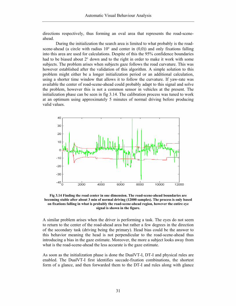
During the initialization the search area is limited to what probably is the road-scene-ahead (a circle with radius 10° and center in (0,0)) and only fixations falling into this area are used for calculations. Despite of this the 95% confidence boundaries had to be biased about 2° down and to the right in order to make it work with some subjects. The problem arises when subjects gaze follows the road curvature. This was however established after the validation of this algorithm. A simple solution to this problem might either be a longer initialization period or an additional calculation, using a shorter time window that allows it to follow the curvature. If yaw-rate was available the center of road-scene-ahead could probably adapt to this signal and solve the problem, however this is not a common sensor in vehicles at the present. The initialization phase can be seen in fig 3.14. The calibration process was tuned to work at an optimum using approximately 5 minutes of normal driving before producing valid values.

Fig 3.14 Finding the road center in one dimension. The road-scene-ahead boundaries are

becoming stable after about 3 min of normal driving (12000 samples). The process is only based on fixations falling in what is probably the road-scene-ahead region, however the entire eye

signal is shown in the figure.

A similar problem arises when the driver is performing a task. The eyes do not seem to return to the center of the road-ahead area but rather a few degrees in the direction of the secondary task (driving being the primary). Head bias could be the answer to this behavior meaning the head is not perpendicular to the road-scene-ahead thus introducing a bias in the gaze estimate. Moreover, the more a subject looks away from what is the road-scene-ahead the less accurate is the gaze estimate. As soon as the initialization phase is done the DualVT-I, DT-I and physical rules are enabled. The DualVT-I first identifies saccade-fixation combinations, the shortest form of a glance, and then forwarded them to the DT-I and rules along with glance


32

time. This block was implemented in ‘State Flow’15, which is more suited for this kind of rule-based protocol. Mini glances (i.e. a sequence of fixations within an area) are joined if they belong to the same area, i.e. glances according to the ISO/SAE standards are formed. Glance times are summed and forwarded to a counter synchronized with an on/off-road-ahead signal, which is the output from the clustering algorithm (see fig 3.13). The counter registers all glances and glance-times belonging to the same task and is then reset for every new task. Before the reset is done however, the data is sent into Matlab workspace for logging purposes. In this case, time-gaps have been used to indicate the beginning and ending of tasks.

The algorithm was designed to run on an xPC (Industrial PC) and all functions are either written in C++ or just a combination of standard Simulink blocks. The validation was however done in the Simulink environment because this made it possible to stream data, which had already been video transcribed, through the model. The model has however been compiled, downloaded and run on an Xpc target to ensure that the code had no errors (Simulink is very forgiving).

3.4 Off-line auto analysis compared with video transcribed analysis The algorithms have been validated to data from the VDM – validation study. This data is available both in SleepyHead format and video transcribed. The video transcription, done at Volvo Technology Corp. in Gothenburg using a Panasonic AG-7355 advanced video player, was conducted according to the ISO 15007-2 and the SAE J-2396 method. Using seven subjects, four measures where compared:

1. Task length

2. Glance frequency

3. Average glance duration

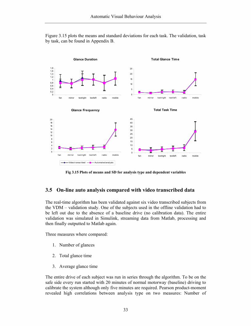
4. Total glance time The amount of non-tracking and bogus data prevented the use of all 14 subjects. This may partly be caused by the early version of eye tracking software used in this study. The validation (presented in appendix B) was preformed task by task with every glance visually confirmed to ensure proper algorithm function. A few fixations were automatically restored using the restoration algorithm that proved to work very well and actually did no miscalculations. Pearson product-moment revealed high correlations between analysis types on all important measures: task length r=0.999, glance frequency r=0.998, average glance duration r=0.816 and total glance duration r=0.995. This is to be compared with the results in ‘Automating driver visual behavior measurement’ (Victor et. al, in press) where the correlations where r=0.991, r=0.997, r=0.732 and r=0.995 respectively.

15 State Flow is a toolbox in Simulink where state/transition diagrams can be created and implemented into Simulink models.


33

Figure 3.15 plots the means and standard deviations for each task. The validation, task by task, can be found in Appendix B.

Glance Duration

00,20,40,60,8

11,21,41,61,8

fan mirror textright textleft radio mobile

Total Glance Time

0

5

10

15

20

25

f an mirror t ext r ight t ext lef t radio mobile

Glance Frequency

02468

101214161820

f an mirror t ext r ight t ext lef t radio mobile

Video t ranscribed Aut omat ed analysis

Total Task Time

0

5

10

15

20

25

30

35

40

45

fan mirror textright textleft radio mobile

Fig 3.15 Plots of means and SD for analysis type and dependent variables

3.5 On-line auto analysis compared with video transcribed data The real-time algorithm has been validated against six video transcribed subjects from the VDM – validation study. One of the subjects used in the offline validation had to be left out due to the absence of a baseline drive (no calibration data). The entire validation was simulated in Simulink, streaming data from Matlab, processing and then finally outputted to Matlab again. Three measures where compared:

1. Number of glances

2. Total glance time

3. Average glance time The entire drive of each subject was run in series through the algorithm. To be on the safe side every run started with 20 minutes of normal motorway (baseline) driving to calibrate the system although only five minutes are required. Pearson product-moment revealed high correlations between analysis type on two measures: Number of


34

glances, r=0.925, and Total glance time, r=0.964. Average glance time, however, did not correlate very well, r=0.301. Figure 3.16 plots the means and standard deviations for each task. The validation, task by task, can be found in Appendix B.

Total Glance Time

0

5

10

15

20

25

30

fan mirror radio textleft textright mobile

Glance Duration

-0,5

0

0,5

1

1,5

2

2,5

3

3,5

4


Glance Frequency

0

2

4

6

8

10

12

14

16

18

20


Video transcribe Real-time analysis

Fig 3.16 Plots of means and SD for analysis type and dependent variables.


35

4 Discussion The results from the validation prove that the algorithms are outstandingly reliable, even when data quality is not at its optimum level i.e. the algorithms are robust to varying noise level and signal accuracy. Also, using ocular motion rules, the algorithm can retrieve fixations that have almost vanished in the signal.

The correlation between analysis methods is very high, in the region of 0.99 (off-line version) for all measures except average glance duration, which is still strong (r=0.82). A low correlation could however be expected from a measure based on two others. It can also have been caused by the difference in sampling rates, mentioned in the paper by Victor et al referred to earlier. The SleepyHead/FaceLAB system runs in 60 Hz whereas the video-transcription was done in 30 Hz. A high correlation between the analyses performed in the current work and the one in Victor et al. fortifies this argument. The preprocessing also proved to worked well. The 15-sample median filter preserved saccade beginnings/terminations while subduing noise and blinks very efficiently.

The combination of the DualVT-I, the DT-I and the rules proved to work beyond expectations. The accuracy of the DualVT-I and the reliability of the DT-I in collaboration with the physical rules for eye movements formed an algorithm that is robust to temporary sensor confidence drops and high noise levels. The one question mark is if new versions of FaceLAB, which is a smart sensor i.e. the output is the result of calculations made in a software loop, will have different signal properties. If this is the case the algorithms will need to be re-verified, perhaps changing some of the thresholds. However the only difference that could be expected from a new version is better performance, meaning more accuracy and less noise allowing better measurements in even worse environments such as tunnels and bright sunlight. Also, a first step towards a real-time algorithm is taken. It has been shown that it is possible to have robust and reliable real-time glance detection. A prototype has been developed and simulated. The simulation revealed high correlations on two measures (number of glances and total glance time). The correlation for average glance time was however low (r=0.301). Keeping in mind that the real time algorithm cannot differ a glance towards the mirror from one to the radio, all measures could be expected to be rather low. It is my belief that the real-time algorithm can be made as accurate as the off-line version. This will be achieved by identifying the vehicle objects most commonly looked at during driving i.e. the interior mirror, side mirrors, instrument cluster and center stack. These objects are fairly separated in the vehicle (they will not be mixed up with each other) and it would only take one or two glances in the area that is defined as the most probable area for one of those objects to start an initiation phase for this particular object. The objects most commonly looked at are the ones contributing the most to this error and these are also the ones that are the easiest to detect. The schedule for this work did, however, not allow this to happen.


36

Since no other data set is video transcribed or in any other way analyzed16 it has only been used for testing different algorithm parts e.g. the real-time initialization. However, this work has opened the door for the analysis of this data. This will also be done in PhD work at Volvo Technology Corp.

16 I.e. not with respect to any temporal measures.


37

5 Conclusions A robust hybrid algorithm that works according to the definitions and measures in the ISO 15007-2 and SAE J-2396 standards have been developed. The method is substantially faster than video transcription, one hour of data takes about one day to video transcribe compared to a few minutes with the algorithms which also automatically adapts to the present noise level. In sum:

1. A preprocessing median filtering length of 15 samples was chosen and proved

to give good performance.

2. A median filter with 20 samples is used on noisy signal parts where, according to the ocular rules, there should be a fixation. This calms the signal enough to detect the fixation.

3. A robust hybrid of two fixation/saccade detection algorithms, which adapts to

the present noise level, and the decision algorithm has been developed and tuned for 60 Hz SleepyHead/FaceLAB data.

4. Physical rules for eye movements, as described in section 1, are implemented

as a smart decision-making and controlling algorithm.

5. An automatic and robust clustering method that requires a minimum of interaction has been developed for task analysis.

6. A real-time version of the algorithm has been developed and validated.

7. The real-time version of the algorithm uses a novel framework which

segments glances into the “road-straight-ahead” or “other” categories. 8. All measures in the ISO/SAE have been implemented.

This thesis opens doors for several interesting in-vehicle product applications, which could make use of eye movement data, to be tested in a real on-road environment. For example: workload estimation, attention estimation, drowsiness detection, adaptive interfaces, adaptive warnings etc. Also, it has made FaceLAB a tool that easily could be used in any study where eye movements are of interest i.e. it now produces glance statistics rather than “just” eye movement signals Examples of this are ergonomic evaluations, HMI studies, studies of cognitive workload, distraction, drowsiness etc. Thus,

a new path into the drivers mind has been opened.


38

6 Future work There are still a few manual steps to carry out such as loading and saveing data, visually inspecting the segmentation and occasionally adjusting the world model. This is especially the case with direct sunlight into the cameras witch scatters fixations over large areas that sometimes even ‘melts’ clusters together. Thus, as Facelab becomes more robust and accurate some of these steps will no longer be necessary and perhaps batch processing will be possible. The ultimate goal is to have a real-time algorithm that works robustly and intelligently to provide future vehicles (and researchers) with as much usable information as possible from the driver’s eyes. The real-time algorithm needs to be further developed to be able to classify several objects robustly and smartly. Especially the real-time adaptation of world model objects to the real world needs improvement but also the logging of events and data. One interesting approach is to implement target areas as HMM states. Introducing this statistical approach target classification would probably be enhanced, as it would make the target area boundaries more floating. One interesting idea is to have world model areas pop up when ever fixations are registered outside or at a distance away from the other objects, a dynamic world model. The world model could use this history of objects to calibrate it self and make intelligent decisions i.e. an entirely task driven identification of objects. When it comes down to the detection algorithms perhaps other sensor information could be utilized. In modern cars the CAN17 bus is full of sensor signals that might be useful to estimate gaze direction when tracking fails i.e. the steering angle, turn indicators, speed, button presses etc. This could also provide information about the traffic environment and thus optimize segmentation parameters for specific traffic environments e.g. country, suburban and city traffic. A rather successful approach to recognize large scale driving patterns has been done in the master thesis ‘Real-time Recognition of Driver Behavior’ by Engström (2000).

A few other WFHM-filters could be tested to see if there is a better way to reduce noise in the beginning of fixations away from the road, this is where the restoration algorithm is used. The flora of filters seems to be enormous.

A different way to support the algorithm could be the fact that a subject’s head often moves in the same direction as the eyes, at least for lateral gaze (Uemura et al. 1980). The problem with this approach is due to the individual differences in subjects. Some subjects virtually do not move their head at all while some always do. Still this might be a nice way to aid the segmentation when gaze is noisy. In the real-time algorithm a prediction of the next six samples would increase speed with 100 ms. Wu and Bahill (1989) has shown that saccadic signals can be predicted, at least a few points, with very small errors using a five point quadratic predictor. Speed is of the highest importance for a real-time algorithm but since FaceLAB at the present has a two seconds delay the 100 ms will not do much of a difference.

17 The CAN bus (Control Area Network) is the central information highway in most modern cars.


39

In the light of what is mentioned above, it is clear that the development of these algorithms can go on for a long time. One development that is already under way is an algorithm GUI, called ‘Visual Demand Measurement Tool’ or simply ‘VDMTool’. The purpose of this program is to make the analysis tools easy to use for anyone who whishes to analyze eye-movements. A screenshot of VDMTool can be seen in fig 6.1.

Fig 6.1 VDMTool screen dump during analysis of an RTI task

SleepyHead/FaceLAB could also do with some enhancements. The tracking volume needs to be big enough to track the driver head in all positions possible while driving and something could be done about the sun shining straight into the camera lenses. Also, to make the real-time algorithms useful, the lag time between eye movement and outputted data has to be minimized (as mentioned earlier). For drowsiness applications maybe half a second is fast enough but for attention estimates a maximum delay of 60-100 ms is required.


40

References Cecchin, T., Sauter, D., Brie, D. and Martin, B. 1990. On-line Separation of Smooth Pursuit and Saccadic Eye Movements, Annuall International Confereence of the IEEE Engineering in Medicine and Biology Society, vol. 12, no. 2, 777-778, 1990 Carpenter, R. H. S., 1998, Movements of the Eyes, 2nd Edition. Pion: London Castet, E., Masson, G. S., 2000, Motion perception during saccadic movements, Nature neuroscience vol 3, no 2, 2000. Engström, J., Johansson, E. and Victor, T. 2002, Vigilance Simulator study at Volvo Technological Development, Gothenburg, Sweden, In preparation Engström, J 2000, Real-time Recognition of Driver Behavior, Volvo Technological Development, Gothenburg, Sweden and School of Cognitive and Computing Sciences, University of Sussex, Brighton, UK Gu, J., Meng, M., Cook, A. and Faulkner M. G. 2000. Analysis of Eye Tracking Movements using FIR Median Hybrid Filters, Eye Tracking Research and Application Symposium 2000, Palm Beach Gardens, FL, USA Harbluk, J. L., Noy, Y. I. 2002. The Impact of Cognitive Distraction on Driver Visual Behaviour and Vehicle Control, Ergonomics Division, Road Safety Directorate and Motor Vehicle Regulation Directorate, Minister of Transport Canada, 2002. ISO 1999, Road Vehicles – Measurement of driver visual behavior with respect to transport information and control systems – Part 2: Equipment and procedures. ISO/CD 15007-2 Juhola, M., 1990. Median Filtering is appropriate to signals of saccadic eye movements. Comp. Biol. Med.,1991, vol 21, No ½, pp 43-49, Great Britain Juhola, M., Jäntti, V. and Aantaa, E. 1985. Analysis of Saccadic Eye Movements with a Microcomputer, Journal of Biomedicine, vol 8, July, England Juhola, M., Jäntti, V., Pyykkö, I., Magnusson, M., Schalen, L. and Åkesson, M. 1985. Detection of saccadic eye movements using a non-recursive adaptive digital filter, Computer Methods and Programs in Biomedicine, no. 21, p. 81-88, Elsevier Science Publishers B.V., 1985 Liu, A., 1997, What the Driver’s Eye Tells the Car’s Brain. Cambridge Basic Research, Cambridge, USA Marble, A. E. , McIntyre, C. M., Hastingss-James, R., Hor, C. W. A comparison of digital algorithms used in computing the derivative of left ventricular pressure. IEEE Trans. Biomed. Eng. 28, 524-529 1981


41

Matsumoto, Y. and Zelinsky, A., 2000, An Algorithm for Real-time Vision Implementation of Head Pose and Gaze Direction Measurement. Rabiner, L. R., 1989, A tutorial on hidden Markov models and selected applications in speech recognition. Proceedings of the IEEE, 1989, 77, 257-286 Recarte, M. N., Nunes, L. M., 2000. Effects of Verbal and Spatial Imagery Tasks on Eye Fixations While Driving, Journal of Experimental Psychology: Applied, vol 6, no 1, p 31-43, 2000. Ross. T., 2002. Safety first, Transport Technology Ergonomics Center, Loughborough University, UK. Traffic Technology international, Feb/Mar 2002. SAE 1999, Definition and Experimental Measures Related to the Specification of Driver Visual Behavior Using Video Based Techniques. Draft Recommended practice, SAE J-2396 Salvucci, D. and Goldberg, J. 2000, Identifying Fixations and Saccades in Eye-tracking Protocols. Proceedings of Eye Tracking Research & Applications Symposium 2000. Palm Beach Gardens, FL, USA. SeeingMachines 2001, User manual for faceLAB 1.0, Document version 1.0.0, www.seeingmachines.com SeeingMachines 2000, Provisional patent application, 2000 Fuchuan, S. and Lingyu, C. 1995. Identification of Fixations in Reading Eye Movements by a Multi-.layer Neural Network. IEEE 1995 Treat, J. 1979. Tri-level Study of the Causes of Traffic Accidents. Final Report, volume 1. Technical Report Federal Highway Administration, US DOT, 1979 Victor, T., Blomberg, O and Zelinsky, A., (in press). Automating driver visual behavior measurement, Vision in veihcals 9 Uemura, T., Arai, Y., and Shimazaki, C., 1980. Eye-Head Coordination During Lateral Gaze in Normal Subjects.Acta oto-laryngologica, 90, p 191-198, 1980, Stockholm Scandinavian University Press Värri, A., Hirvonen, K., Häkkinen, V., Hasan, J. And Loula Pekka 1996, Nonlinear eye movement detection method for drowsiness studies. International Journal of Bio-Medical Computing, 1996, 43, 227-242 Wang, J. S., Knipling, R. R., and Goodman, M. J. 1996. The Role of Driver Inattention in Crashes: New Statistics from the 1995 Crashworthiness Data System, Proceedings of the 40th Annual Meeting of the Association of Automotive Medicine, Vancouver, October 1996.


42

Wu, C-Y. and Bahill, A. T. 1989. Block-Processing Adaptive Filter for Human Eye Movements. Computers industrial Engineering, vol. 17, nos 1-4, p 496-501, Pergamon Press plc, Great Britain, 1989 Wyatt, H. J. 1997. Detecting saccades with jerk, Vision Reasearch 38, 1998, 2147-2153.

-I-

Appendix A: FaceLAB and SleepyHead signals

SleepyHead v 3.1 Signal name Dimension Precision Frame number n-by-1 unsigned integer 32 bit Frame time s n-by-1 integer 32 bit Frame time ms n-by-1 unsigned integer 16 bit Delay ms n-by-1 unsigned integer 32 bit Tracking n-by-1 unsigned integer 8 bit Blinking n-by-1 integer 8 bit Head position filtered n-by-3 float 32 bit Head rotation filtered n-by-3 float 32 bit Head pose confidence n-by-1 float 32 bit Gaze rotation filtered n-by-2 float 32 bit Gaze confidence n-by-1 float 32 bit Attention n-by-2 float 32 bit Attention confidence n-by-1 float 32 bit Left upper cover n-by-1 float 32 bit Left opening n-by-1 float 32 bit Left lower cover n-by-1 float 32 bit Left lid confidence n-by-1 float 32 bit Right upper cover n-by-1 float 32 bit Right opening n-by-1 float 32 bit Right lower cover n-by-1 float 32 bit Right lid confidence n-by-1 float 32 bit Perclos70 n-by-1 float 32 bit Perclos80 n-by-1 float 32 bit Blink frequency n-by-1 float 32 bit Blink duration n-by-1 float 32 bit Blink opening time n-by-1 float 32 bit Blink closing time n-by-1 float 32 bit Object index n-by-1 integer 32 bit

-II-

FaceLAB v 1.0 Signal name Dimension Precision Frame number n-by-1 unsigned integer 32 bit Time n-by-1 float 32 bit Tracking n-by-1 integer 16 bit Blinking n-by-1 integer 16 bit Head position raw n-by-3 float 32 bit Head position filtered n-by-3 float 32 bit Head rotation raw n-by-3 float 32 bit Head rotation filtered n-by-3 float 32 bit Head pose confidence n-by-1 float 32 bit Gaze rotation raw n-by-2 float 32 bit Gaze rotation filtered n-by-2 float 32 bit Gaze confidence n-by-1 float 32 bit Eye opening raw n-by-1 float 32 bit Eye opening filtered n-by-1 float 32 bit Object index n-by-1 integer 32 bit

-III-

Appendix B: Validation of automated analysis Video transcribed data Automated analysis

Sub-ject Task

Glance frequency

Total glance duration

Average glance dur.

Total task duration

Glance frequency

Total glance duration

Average glance duration

Total task

duration

1 mirror 3 1,310 0,437 8,440 TRACKING FAILURE

1 textleft 5 5,640 1,128 11,640 4 5,683 1,421 10,850

1 textleft 2 1,590 0,795 5,530 2 1,350 0,675 5,300

1 textright 2 2,240 1,120 2,600 2 2,683 1,342 2,683

1 textright 2 2,300 1,150 2,700 2 2,250 1,125 2,667

1 mobile 11 8,000 0,727 17,340 11 8,483 0,771 17,317

1 mobile 20 20,670 1,034 43,340 20 20,633 1,032 42,917

1 fan 4 2,360 0,590 6,400 4 2,383 0,596 6,417

1 fan 2 2,400 1,200 4,000 2 2,500 1,250 4,033

1 radio 5 3,330 0,666 11,240 5 3,550 0,710 9,950

1 radio 7 4,530 0,647 15,360 7 4,600 0,657 15,267

2 mirror 3 1,700 0,567 5,800 2 1,583 0,792 4,083

2 mirror 1 1,000 1,000 1,000 1 0,983 0,983 0,983

2 textleft 2 2,760 1,380 3,300 2 1,100 0,550 1,967

2 textright 1 1,800 1,800 1,800 1 1,733 1,733 1,733

2 textleft 1 2,040 2,040 2,040 1 0,750 0,750 0,750

2 textright 2 3,030 1,515 4,030 2 1,317 0,658 3,950

2 mobile 11 13,680 1,244 28,160 10 11,567 1,157 26,100

2 mobile 9 13,360 1,484 18,040 8 12,633 1,579 15,567

2 fan 3 2,630 0,877 5,160 3 2,683 0,894 5,150

2 fan 2 1,560 0,780 1,930 2 1,517 0,758 1,900

2 radio 2 1,300 0,650 3,830 2 1,300 0,650 3,883

2 radio 1 0,570 0,570 0,570 1 0,617 0,617 0,617

4 mirror 1 0,500 0,500 0,500 1 0,533 0,533 0,533

4 mirror 3 2,030 0,677 3,600 3 1,917 0,639 3,550

4 textleft 4 2,920 0,730 4,630 4 2,833 0,708 4,600

4 textleft 1 0,830 0,830 0,830 1 0,833 0,833 0,833

4 textright 4 2,190 0,547 5,130 4 2,100 0,525 5,117

4 textright 2 1,300 0,650 1,700 2 1,267 0,633 1,667

4 mobile 14 11,250 0,804 20,630 14 11,383 0,813 20,567

4 mobile 15 11,620 0,775 23,460 15 11,650 0,777 23,500

4 fan 4 1,850 0,463 4,130 4 1,917 0,479 4,100

4 fan 3 1,790 0,597 3,860 3 1,733 0,578 3,900

4 radio 3 1,560 0,520 15,300 3 1,667 0,556 15,367

4 radio 3 1,970 0,657 7,800 3 1,883 0,628 7,800

7 mirror 2 1,300 0,650 2,070 2 1,300 0,650 2,100

7 mirror 1 1,230 1,230 1,230 1 1,200 1,200 1,200

7 textleft 2 1,980 0,990 2,640 2 2,233 1,117 2,667

7 textright 3 3,930 1,310 8,100 3 4,017 1,339 8,167

7 textright 3 2,570 0,857 3,730 3 2,583 0,861 3,717

7 mobile 14 13,740 0,981 28,770 13 13,633 1,049 28,700

7 mobile 12 12,640 1,053 23,630 12 12,783 1,065 23,517

-IV-

7 fan 2 2,310 1,155 2,940 2 2,267 1,133 2,900

7 fan 3 3,440 1,147 5,040 3 3,317 1,106 4,817

7 radio 4 2,760 0,690 7,200 4 2,650 0,663 7,183

7 radio 2 1,700 0,850 2,870 2 1,833 0,917 3,000

9 mirror 3 3,860 1,287 5,000 3 3,883 1,294 4,967

9 mirror 4 2,870 0,717 8,770 4 3,000 0,750 8,867

9 textleft 2 3,470 1,735 3,940 2 3,250 1,625 3,850

9 textleft 3 4,670 1,557 5,600 3 4,567 1,522 5,483

9 textright 4 6,410 1,603 7,870 4 6,450 1,613 7,950

9 textright 3 6,340 2,113 7,240 3 4,230 1,410 5,217

9 mobile 15 27,280 1,819 35,940 15 27,250 1,817 35,817

9 mobile 12 24,910 2,076 31,030 12 24,983 2,082 31,000

9 fan 3 4,800 1,600 5,900 3 3,400 1,133 5,800

9 fan 2 4,010 2,005 4,940 2 1,900 0,950 4,833

9 radio 3 6,100 2,033 8,470 3 5,950 1,983 8,350

9 radio 3 5,170 1,723 6,930 2 3,733 1,867 5,100

10 mirror 2 1,710 0,855 10,440 2 0,900 0,450 10,430

10 textleft 4 2,570 0,642 9,440 4 2,750 0,688 9,500

10 textleft 3 2,470 0,823 7,930 3 2,533 0,844 7,950

10 textright 4 3,560 0,890 10,260 4 3,517 0,879 10,167

10 textright 3 2,330 0,777 7,860 3 2,317 0,772 7,867

10 mobile 12 9,720 0,810 17,430 12 9,183 0,765 16,667

10 mobile 11 11,390 1,035 29,860 TRACKING FAILURE

10 fan 2 1,460 0,730 3,100 2 1,400 0,700 3,117

10 fan 2 1,290 0,645 3,630 2 1,233 0,617 3,500

10 radio 2 1,360 0,680 6,530 2 0,900 0,450 6,083

10 radio 1 0,630 0,630 0,630 1 0,483 0,483 0,483

14 mirror 2 0,900 0,450 2,660 2 1,083 0,542 2,667

14 mirror 1 0,670 0,670 0,670 1 0,700 0,700 0,700

14 textleft 3 2,370 0,790 6,640 TRACKING FAILURE

14 textleft 1 0,730 0,730 0,730 1 0,300 0,300 0,300

14 textright 2 1,230 0,615 2,130 2 1,250 0,625

14 textright 1 0,840 0,840 0,840 1 0,750 0,750 0,750

14 mobile 12 7,900 0,658 29,400 12 7,333 0,611 29,300

14 mobile 24 20,400 0,850 62,800 24 19,483 0,812 62,617

14 fan 3 1,660 0,553 4,230 3 1,717 0,572 4,150

14 fan 3 1,770 0,590 5,470 3 1,660 0,553 5,433

14 radio 4 2,270 0,567 5,840 4 2,217 0,554 5,817

14 radio 4 1,750 0,438 3,940 4 1,733 0,433 5,383

Pearson product

movementGlance

frequencyTotal glance

duration Average glance

duration Task

duration

Correlation 0,9984 0,9946 0,8165 0,9986

-V-

Variance analysis

avg. glance std. glance avg. total gla-

std. total gla- avg. avg. std. avg. avg. Task std. Task

Task frequency frequency duration duration glance dur. glance dur. duration duration

Mirror discrimination 2,09 1,000 1,570 0,970 0,76 0,27 3,92 3,34Text left instrument 2,48 1,190 2,490 1,470 1,01 0,43 4,76 4,43Text right instrument 2,57 1,000 2,430 1,600 1,07 0,44 4,63 2,92

Adjust fan level 2,71 0,710 2,250 0,870 0,87 0,37 4,31 1,20

Adjust radio 3,11 1,590 2,430 1,630 0,80 0,47 6,81 4,49

SMS message 13,70 4,020 14,720 6,110 1,10 0,43 29,02 12,26

-VI-

På svenska Detta dokument hålls tillgängligt på Internet – eller dess framtida ersättare – under en längre tid från publiceringsdatum under förutsättning att inga extra-ordinära omständigheter uppstår.

Tillgång till dokumentet innebär tillstånd för var och en att läsa, ladda ner, skriva ut enstaka kopior för enskilt bruk och att använda det oförändrat för ickekommersiell forskning och för undervisning. Överföring av upphovsrätten vid en senare tidpunkt kan inte upphäva detta tillstånd. All annan användning av dokumentet kräver upphovsmannens medgivande. För att garantera äktheten, säkerheten och tillgängligheten finns det lösningar av teknisk och administrativ art.

Upphovsmannens ideella rätt innefattar rätt att bli nämnd som upphovsman i den omfattning som god sed kräver vid användning av dokumentet på ovan beskrivna sätt samt skydd mot att dokumentet ändras eller presenteras i sådan form eller i sådant sammanhang som är kränkande för upphovsmannens litterära eller konstnärliga anseende eller egenart.

För ytterligare information om Linköping University Electronic Press se förlagets hemsida http://www.ep.liu.se/ In English The publishers will keep this document online on the Internet - or its possible replacement - for a considerable time from the date of publication barring exceptional circumstances.

The online availability of the document implies a permanent permission for anyone to read, to download, to print out single copies for your own use and to use it unchanged for any non-commercial research and educational purpose. Subsequent transfers of copyright cannot revoke this permission. All other uses of the document are conditional on the consent of the copyright owner. The publisher has taken technical and administrative measures to assure authenticity, security and accessibility.

According to intellectual property law the author has the right to be mentioned when his/her work is accessed as described above and to be protected against infringement.

For additional information about the Linköping University Electronic Press and its procedures for publication and for assurance of document integrity, please refer to its WWW home page: http://www.ep.liu.se/ © [Petter Larsson]

Automatic Visual Behavior Analysis - DiVA portal19307/FULLTEXT01.pdf · Automatic Visual Behavior...

Documents

Transcript of Automatic Visual Behavior Analysis - DiVA portal19307/FULLTEXT01.pdf · Automatic Visual Behavior...