Calhoun: The NPS Institutional Archive

Theses and Dissertations Thesis Collection

1992-12

Automatic pulse shaping with the AN/FPN-42 and

AN/FPN-44A Loran-C transmitters

Bruckner, Dean C.

Monterey, California. Naval Postgraduate School

http://hdl.handle.net/10945/38503

&VAL POSTGRADUATE SCHOOLMonterey, California

,A257 860

DTICk ELECTE INB 0 4.1992. fliADECEO4 THESIS

AUTOMATIC PULSE SHAPING WITH THEAN/FPN-42 AND AN/FPN-44ALORAN-C TRANSMITTERS

by

Dean C. Bruckner

December 1992

Thesis Advisor: Murali TummalaSecond Reader- Roberto Cristi

Approved for public release; distribution is unlimited.

92-30839

REPORT DOCUMENTATION PAGEI& REPORT SECURITY CLASSIFICATON UNCLASSIFIED 1b. RESTRICTIVE MARKINGS

2a SECURITY CLASSIFICATION AUTHORITY 3. DISTRIBUTION/AVAILABiLITY OF REPORT2b. DECLASSIFICATIONDOWNGRADING SCHEDULE Approved for public release;distribution is unlimited

4. PERFORMING ORGANIZATION REPORT NUMBER(S) 5. MONITORING ORGANIZATION REPORT NUMBER(S)

.MOFP-FRmINRGAIZA T ON 1b. OFFICE SYMBOL 7a. NAME OF MONITORING ORGANIZATION%aostgraoua e 0Cifcnod applicable) Naval Postgraduate School

I EC

6c. ADDRESS (Ciy, State, and ZIP Code) 7b. ADDRESS (City, State, and ZIP Code)

Monterey, CA 93943-5000 Monterey, CA 93943-5000

8 NAME OF FUNDING/SPONSORING 8b. OFFICE SYMBOL 9. PROCUREMENT INSTRUMENT IDENTIFICATION NUMBERORGANIZATION (if applicable)

8c. ADDRESS (City, State, and ZIP Code) 10. SOURCE OF FUNDI01G NUMBERSPROGRAM PROJECT I TASK WORK UNITELEMENT NO. NO. NO. ACCESSION NO.

11. TITLE (Include Secuity Classification)AUTOMATIC PULSE SHAPING WITH THE AN/FPN-42 AND AN/FPN-44A LORAN-C TRANSMITTERS (U)g.FMPF.J SN/ AUTHaR(S)

c soer,ea AUNT

~eY~QERORT '13b.T TIME COWRED E1DT CTOaUNT a) ~ PG09NANJ 10/92 CAEOF REPSn, 19I FROM 07 TO 1 ctober R M9 COUNT

16. SUPPLEMENTARY NOTATION The views expressed in this thesis are those of the author and do not reflect theofficial policy or position of the Department of Defense or the United States Government.

17. COSATI CODES 18. SUBJECT TERMS (Continue on reverse if necessary and identify by block number)

FIELD GROUP SUB-GROUP Loran, pole-zero modeling, ARMA modeling, steepest-descent,"-,ule-Walker, Shank's, VXlbus

19. ABSTRACT (Conhnue on reverse if necessa. and idengf by block number)Automatic pulse shape control is simulated for the AN/FPN-42 and AN/FPN-44A tube type transmitters. A

linear, time invariant (LTI) pole-zero model is developed for each transmitter at a typical operating point using theleast squares modified Yule- Walker method and Shank's method. LTI models for a range of operating points arecatenated to represent observed nonlinear behavior, and observed time variations are added. After these combinedmodels are tested, a linear controller based on the method of steepest descent is implemented. These models, thecontrol algorithm and transmitter system details such as power supply droop, dual rating and noise are then incor-porated into a MATLAB simulation program.

In a variety of realistic tests the control algorithm successfully shaped the Loran-C pulse, except that zero-crossing times were not always in tolerance and the algorithm showed a sensitivity to noise. The algorithm controlledEnvelope-to-Cycle Difference, produced an entire Phase Code Interval of pulses while compensating for droop andphase code bounce, and produced a near- optimal transmitter drive waveform for the transmitter/antenna systemusing the dummy load.

20. DISTRIBUTION/AVAILABILITY OF ABSTRACT 21. ABSTRACT SECURITY CLASSIFICATION

[ UNCLASSIFIED/UNLIMITED [] SAME AS RPT. Q3 DTIC USERS UNCLASSIFIEDfta.N AI OFMRESPONSIBLE INDIVIDUAL 22. u aoudeArea Coe) 2 2 CEF'jJ SYMBOL

a " la. I9149d Are code)

Approved for public release; distribution is unlimited

Automatic Pulse Shaping with the AN/FPN-42 and AN/FPN-44ALoran-C Transmitters

by

Dean C. BrucknerLieutenant, United States Coast Guard

B. S., United States Coast Guard Academy, 1985

Submitted in partial fulfillment of therequirements for the degree of

MASTER OF SCIENCE IN ELECTRICAL ENGINEERING

from the

NAVAL POSTGRADUATE SCHOOL

December 1992

Author:D

Approved by: Murali Tummala, Thesis Advisor

.

and Computer Engineering

ii

ABSTRACT

Automatic pulse shape control is simulated for the AN/FPN-42 and AN/FPN-

44A tube type transmitters. A linear, time invariant (LTI) pole-zero model is de-

veloped for each transmitter at a typical operating point using the least squares

modified Yule-Walker method and Shank's method. LTI models for a range of op-

erating points are catenated to represent observed nonlinear behavior, and observed

time variations are added. After these combined models are tested, a linear con-

troller based on the method of steepest descent is implemented. These models, the

control algorithm and transmitter system details such as power supply droop, dual

rating and noise are then incorporated into a MATLAB simulation program.

In a variety of realistic tests the control algorithm successfully shaped the

Loran-C pulse, except that zero-crossing times were not always in tolerance and the

algorithm showed a sensitivity to noise. The algorithm controlled Envelope-to-Cycle

Difference, produced an entire Phase Code Interval of pulses while compensating

for droop and phase code bounce, and produced a near-optimal transmitter drive

waveform for the transmitter/antenna system using the dummy load.

Accesion ForNTIS CR,P&I011IC TALBUranourced Ltjstificatioi ............

B y ............................................. ...

DAt: ibutiol IA vi_.ti.j)1 lY G 3 F

Soist ;.ic-

'H4

TABLE OF CONTENTS

INTRODUCTION ............................. 1

II. AN OVERVIEW OF LORAN-C ..................... 3

A, LORAN-C IN BRIEF ......................... 3

1. H istory . . . . . . . . . . . . . . . . . . . . . . . . . . . . . . . 3

2. How Loran-C Works ....................... 4

3. The Accuracy, Reliability and Availability of Loran-C ..... 8

4. Loran-C's Future ......................... 9

B. THE LORAN-C SIGNAL ....................... 9

1. The Individual Loran Pulse ................... 9

a. General Description ..................... 9

b. Specification: Individual Pulse (Four Tests) .......... 11

2. The Loran-C Pulse Group .................... 15

a. Format of the Pulse Group ................. 15

b. Multipulse Trigger ...................... 16

c. Pulse Group Phase Coding ..................... 17

d. Transmitter Power Supply Droop .................. 18

e. Specification: Uniformity of Pulses Within a Group (ThreeTests) . . . . . . . . . . . . . . . . . . . . . . . . . . . . . 19

3. Blink and "Out-of-tolerance" . .................. 20

4. Dual-rating and Dual-rate Blanking ............... 22

5. Frequency Spectrum Requirements ................... 23

C. PRODUCING THE SIGNAL .......................... 23

1. The Loran Transmitter ............................ 23

iv

a. Types of Transmitters .......................... 23

b. Transmitter Loads ............................ 24

c. Normal Loran Operating Procedures ............... 25

d. Nonlinear and Time-Varying Behavior of Tube Transmitters 26

e. Transmitter Phase Code Balance .................. 27

2. Transmitter Drive Waveforms and Typical Outputs ........ 27

3. Controlling the Pulse Shape ........................ 28

D. THE ELECTRONIC EQUIPMENT REPLACEMENT PROJECT(EERP) AND THE PURPOSE OF THIS RESEARCH ........ 32

1. The EERP and its Plan 1 ...... .................... 32

2. The VXIbus Based Loran-C Transmitter and Control System 33

3. Purpose of This Research ...... .................... 34

a. Primary goal: A Control Algorithm ................ 34

b. Necessary Tool: A Computer Simulation Program . . . . 35

III. MODELING THE AN/FPN-42 AND 44A LORAN-C TRANSMITTERS 37

A. INTRODUCTION ................................ 37

B. THE MODELING APPROACH ........................ 37

1. Discrete-Time Representation ........................ 37

2. Data from the '42 and '44A transmitters ................ 38

a. Data Collection ...... ....................... 38

b. Effects of Noise and Quantization ................. 38

3. Linearity and Time Invariance ....................... 41

a. Initial Assumption: Linear, Time Invariant (LTI) WithinEach Pulse .......................... 41

b. Verifying the Assumption ....................... 41

c. Adapting the Assumption to Nonlinear and Time-VaryingBehavior ....... ........................... 42

4. Time-Domain Pole-Zero Modeling .................... 43

v

wnwwwV

a. Single LTI System ............................ 43

b. Catenated LTI Models .......................... 44

C. IDENTIFYING THE SYSTEM ..... ................... 45

1. Frequency-Domain Deconvolution and its Numerical Problem 45

2. Removing Spurious Peaks with Median Smoothing ....... 46

D. A POLE-ZERO MODEL OF THE SYSTEM UNIT SAMPLERESPONSE ('42 WITH ANTENNA SIMULATOR) .......... 51

1. Sampling Frequency Considerations ............... 51

2. Technique for Estimating the AR Parameters: The Least SquaresModified Yule-Walker Method .................. 52

3. Technique for Estimating the MA Parameters: Shank's Method 54

4. The Pole-Zero Model ....................... 56

5. Two Criteria for Selecting Model Order ............. 57

E. NONLINEAR, TIME-VARYING MODEL OF THE AN/FPN-42TRANSMITTER ........................... 61

1. Representing Nonlinearities by Moving Poles and Zeros .... 61

a. Changes in the Positions of Poles and Zeros Caused byChanges in TDW Shape ................... 61

b. Assigning Poles and Zeros by Parameter E, ........ .. 61

c. Performance of the Catenated Model ............... 65

2. Representing Time Variations by Changing PolynomialCoefficient co . . . . . .. . . . . . . . . . . . . . . . . . . . . .. . . . . . 67

a. Changes in the Positions of Poles and Zeros Caused byTime Variations ....................... 67

b. Moving Poles and Zeros Using Coefficient co . . . . . . . . . 67

c. Simulating Slow Drifts Using an AR2 Random Process. . 69

3. The Combined Nonlinear, Time Varying Model .......... 69

4. Adding the Dummy Load to the Combined Model ....... .72

F. NONLINEAR, TIME-VARYING MODEL OF THE AN/FPN-44ATRANSMITTER ........................... 75

vi

IV. THE STEEPEST DESCENT ALGORITHM .............. 81

A. INTRODUCTION ........................... 81

B. PULSE SHAPE CONTROL IN LORAN-C ............. 81

C. THE STEEPEST DESCENT ALGORITHM ............ 82

1. Derivation ............................. 82

2. Advantages and Limitations ................... 85

D. CONTROLLING PULSE SHAPE IN THE COMBINED MODELUSING THE STEEPEST DESCENT ALGORITHM .......... 86

V. SIMULATION PROGRAM AND RESULTS .............. 95

A. INTRODUCTION ........................... 95

B. THE SIMULATION PROGRAM ................... 95

1. Structure . . . . . . .. . . . . .. .. . . . . . . . . . . . .. 95

2. Explanation of Features Appearing on Main Menu ........ 95

a. M ain M enu .......................... 95

b. Transmitter Selection .................... 97

c. Transmitter Load ...................... 98

d. Sampling Frequency ..................... 98

e. Local ECD .......................... 99

f. Amplitude Resolution and System Noise ............ 99

g. Transmitter Imbalance ................... 101

h. Reset Transmitter ...................... 101

i. Pulses to Control ...................... 102

j. Pulses to Analyze ... ................... 102

k. Number of Iterations .................... 104

1. Transmitter Drift ...................... 105

m. Transmitter Switch ..................... 105

vii

n. Display Method ............................. 105

o. Control Algorithm ............................ 107

p. Display/Change Current Parameters .............. 107

q. Access Keyboard ............................ 108

3. Explanation of Features Not Appearing in the Main Menu . . 108

a. Simulating Power Supply Droop .................. 108

b. Simulating Dual-Rated Operation ................ 110

c. Exponential Scaling of TDW Amplitudes ........... 114

C. RESULTS ........ ............................... 114

1. Realistic Simulation of the AN/FPN-42 ................ 114

2. Realistic Simulation of the AN/FPN-44A .............. 120

3. Controlling ECD ................................ 120

4. Performance Improvement With Greater Bit Resolution . . . 127

5. Performance Improvement with Less Noise ............. 128

6. Behavior Following a Transmitter Switch ............... 129

7. Controlling the Entire PCI ......................... 130

VI. CONCLUSIONS ....... .............................. 133

A. CONCLUSIONS ................................... 133

B. RECOMMENDATIONS FOR FURTHER STUDY .......... 135

APPENDIX A. COMPUTATIONAL METHOD OF ESTIMATING ECD . 137

APPENDIX B. DATA COLLECTION AND FORMATTING .......... 141

APPENDIX C. FITTED CURVES FOR CATENATED MODELS ...... 147

APPENDIX D. SELECTED MATLAB PROGRAM LISTING ........ 169

REFERENCES .................................. 181

INITIAL DISTRIBUTION LIST ......................... 185

viii

LIST OF TABLES

2.1 ZERO-CROSSING TIMES AND TOLERANCES ............ 16

2.2 LORAN-C PHASE CODES ....................... 18

2.3 PULSE-TO-PULSE ECD TOLERANCES ............... 19

2.4 PULSE-TO-PULSE AMPLITUDE TOLERANCES ............ 20

2.5 PULSE-TO-PULSE TIMING TOLERANCES ............... 21

2.6 TYPES OF LORAN TRANSMITTERS .................. 25

3.1 BASIS FOR SELECTING MODEL ORDER, '42 TRANSMITTER 60

3.2 PERFORMANCE IMPROVEMENT, NONLINEAR VERSUSLINEAR MODEL ............................. 66

5.1 AVERAGE SNR, MEASURED DATA PAIRS (ANTENNA) ...... 100

5.2 PROGRAM SETTINGS WHICH REPRODUCE SNR OFMEASURED DATA ........................... 101

5.3 CONTROLLING ECD .......................... 126

5.4 PERFORMANCE IMPROVEMENT WITH GREATER BITRESOLUTION .............................. 128

5.5 PERFORMANCE IMPROVEMENT WITH LESS NOISE ...... 129

ix

LIST OF FIGURES

2.1 Locations of U.S. Loran stations .......................... 5

2.2 Hyperbolic LOPs ........ ............................. 6

2.3 Emission delays ....... .............................. 7

2.4 Ideal Loran pulse ....... ............................. 10

2.5 Loran pulses with three ECDs ............................ 13

2.6 '42 input and output, antenna simulator ..................... 29

"2.7 '44A input and output, antenna simulator ................... 30

2.8 Two pulse generators ....... ........................... 31

2.9 Manual control diagram ....... ......................... 31

2.10 Diagram of the VXIbus based control system .................. 34

3.1 Power spectrum of '42, antenna simulator .................... 39

3.2 H(n) for '42, antenna simulator .......................... 47

3.3 Smoothed H(n) for '42, antenna simulator ................... 49

3.4 Estimated unit sample response; actual and synthetic FR pulses . . 50

3.5 Diagram of Shank's Method ............................. 56

3.6 Pole-zero plot and sequences, '42 LTI model .................. 58

3.7 Pole-zero scatter plot, five LTI models ..... ................. 62

3.8 Fitted curves for inner pole pair. '42 (5 pairs) ................. 64

3.9 Actual and synthetic RF pulses, catenated model .............. 66

3.10 Three TDWs (9 months apart) and pole-zero plot .............. 68

3.11 Slow drift produced by AR2 process ........................ 69

3.12 Fitted curves for inner pole pair, '42 (19 pairs) ................ 71

3.13 Second AR2 coefficient a2(t, E,) .......................... 72

3.14 '42 Input, output and pole-zero model, dummy load ............. 73

3.15 Power spectrum of '44A, antenna simulator ................... 76

1.16 Pole-zero plot and sequences, '44A LTI model ................. 78

x

3 17 '44A input, output and pole-zero model, dummy load ........... 79

4.1 Loran-C pulse shape control strategy ........................ 83

4.2 Testing steepest descent algorithm with '42 (no time variations) . . . 87

4.3 Testing algorithm with time-varying '42 ..................... 89

4.4 Testing steepest descent algorithm with '44A (no time variations) . . 91

4.5 Testing algorithm with time-varying'44A ..................... 93

5.1 Basic structure, simulation program ........................ 96

5.2 Main menu, simulation program .......................... 97

5.3 Polynomial coefficient matrix ........................... 9S

5.4 Transmitter system noise model .......................... 99

5.5 Printout of pulse analysis results .......................... 103

5.6 Options for displaying error convergence .................... 106

5.7 Menu for steepest descent algorithm ........................ 107

5.8 Charging exponential model of power supply voltage ........... 109

5.9 Vector of consecutive rest times, 200 samples ................. 111

5.10 Effect of transient disturbances ..... ..................... 112

5.11 Realistic simulation run, '42 ............................. 115

5.12 Realistic simulation run, '44A ............................ 121

5.13 Algorithm performance after transmitter switch, '42 ............ 130

xi

ACKNOWLEDGMENT

I would like to thank Professors Tummala, Cristi, Therrien, and Chen at the

Naval Fc~tgraduate School for their assistance and advice. LT Tom Johnson, USN,

and LT Chuck Schue, USCG, students at NPS, helped significantly too. Thanks are

also in order to LCDR Greg Kmiecik and all the personnel at the Loran Branch at

the Coast Guard Electronics Engineering Center for the great support during this

project. CAPT Ben Peterson at the Coast Guard Academy, CDR Doug Taggart

at Coast Guard Headquarters (Navigation Systems Branch), and personnel at the

Coast Guard Pacific Area Headquarters and Maintenance and Logistics Command,

Coast Guard Training Center Petaluma, and Coast Guard Loran Station Middle-

town were also helpful. Finally, thanks to my family and friends for their support

and patience.

xii

I. INTRODUCTION

Modernizing old electronic systems has always presented a challenge to design

engineers, and the U.S. Coast Guard's effort to redesign the control system for

its Loran-C transmitters is no exception. Coast Guard engineers have identified

commercially-available hardware to replace much of the old cont:ol equipment. This

new equipment will be easier to maintain and operate and will allow more Loran-C

control functions to be automated. To realize this capability, however, new software

must be developed to perform each function. This is one of the most challenging

aspects of the redesign effort.

One of the most important control functions is shaping the pulse produced by

older classes of Loran transmitters. A Loran receiver uses the envelope of the pulse

to identify a standard zero-crossing; if the envelope is distorted, the receiver may

lock onto the wrong zero-crossing, resulting in a large position error. The software to

shape the pulse automatically requires a reliable algorithm. In this thesis, a control

algorithm based on the method of steepest descent is adapted to meet this need.

In order to test the algorithm fully and to provide a tool for future study, a

detailed MATLAB computer program is developed to simulate two older transmitter

classes, the AN/FPN-42 and AN/FPN-44A. With no documentation available on

the theory behind the design of these transmitters, this is an exercise in system

identification and modeling. With its wealth of linear algebra and signal processing

functions, MATLAB is an ideal operating environment for this work.

Many details of the '42 and '44A transmitter systems and of their operation

affect the shape of the transmitted pulse. To make the simulation a realistic one,

as many of these details as possible are included. Chapter II gives an overview

I

of Loran-C and provides the background needed to understand these details. It

explains each of the pulse shape tests found in the Coast Guard's Specification for

the Transmitted Loran-C Signal [Ref. 1]. In Chapter III, mathematical models for

the '42 and '44A transmitters are developed; in Chapter IV, the control algorithm is

presented. These models and the control algorithm then form the foundation of the

simulation program described in Chapter V. Chapter V also includes results from

a variety of tests performed using the simulation program. Finally, conclusions and

recommendations for further study are given in Chapter VI.

2

II. AN OVERVIEW OF LORAN-C

A. LORAN-C IN BRIEF

1. History

LORAN, short for LOng RAnge Navigation, is a radionavigation sys-

tem developed during World War II by the famous Radiation Laboratory at the

Massachusetts Institute of Technology. The first version, called Loran-A, was used

during the war to guide Allied military ships and aircraft in the North Atlantic and

Pacific Oceans. By war's end, Loran coverage extended over most of the areas in the

North Atlantic and Pacific where U.S. forces operated. Loran-A, with its one to two

nautical mile (Nm) fix accuracy and its range of 600 to 800 miles, was a significant

factor in bringing the war quickly to an end and in preventing the loss of aircraft

because of inaccurate navigation [Ref. 2: p. 153].

After the war, while Loran-A continued to operate, research began on

a similar system called the Cycle Matching Tactical Bombing (CYTAC) navigation

system for the U.S. military. In 1958 the U.S. Coast Guard assumed control of the

CYTAC system, which was renamed Loran-C. By using a lower frequency band of

90 to 110 kHz instead of 1.7 to 2.0 MHz as in Loran-A, greater range was possible.

Also, other technical improvements brought more accurate geographic positioning

[Ref. 3: p. 2-121.

At first, Loran-C was used mainly by the Department of Defense. As

the number and size of ships passing through coastal U.S. waters increased and as

several new radionavigation systems were developed, it became apparent that the

U.S. government should designate one system which it would support. In 1974 the

Secretary of Transportation adopted Loran-C as the official radionavigation system

3

for coastal U.S. waters with a minimum accuracy requirement of 0.25 Nm and a

minimum reliability of ninety-five percent of the time in the Coastal Confluence

Zone (CCZ), essentially the area from the shore out to 50 Nm. By the early 1980s,

the Coast Guard had phased out the last of its Loran-A stations and had extended

Loran-C coverage over the entire CCZ [Ref. 4: p. 12]. In 1990, at the request of

the Federal Aviation Administration, the Coast Guard began a project to extend

Loran-C coverage from coast to coast in the continental U.S. Today the Coast

Guard operates Loran-C stations in the U.S.; its territories; and in "host nations"

such as Italy, Japan and Turkey. In addition, Loran-C stations are operated by other

nations, such as Saudi Arabia, China and Russia. Figure 2.1 shows the locations of

Loran-C stations now operating in the U.S.

2. How Loran-C Works

Like Loran-A, Loran-C is based on time differences (TDs) between the

signals of a master station and one or more secondary stations. Beginning with the

master, each of the stations in the "chain" transmits in turn a sequence of short

pulses. A receiver located in the chain's area of coverage measures and displays the

elapsed time between the signals from each station. The time difference between

the master and secondary indicates that the receiver is located at some point on

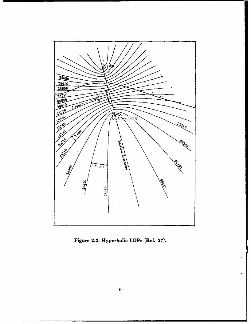
a hyperbolic line of position. A number of time difference lines of position from

one baseline (one master and one secondary station) are shown in Fig. 2.2. When

more stations are added, their time difference lines overlay these and form a grid of

hyperbolic lines. The secondaries, up to four in number, are designated W, X, Y,

and Z. Given two or more lines of position, the receiver "fixes" its position at the

intersection of these lines.

The chain's master and the secondary stations repeat the sequence of

pulses at a fixed rate, according to the Group Repetition Interval (GRI) assigned

4

Figure 2.1: Locations of U.S. Loran stations.

to the chain when it was first installed. Assigned GRIs vary from 40,000 to 99,990

microseconds, so the chain's cycle may repeat anywhere from 10 to 20 times each

second. By convention in Loran-C, elapsed time is generally described in microsec-

onds or nanoseconds, but not in milliseconds. Each station in a chain transmits

its own pulse sequence with the same GRI. Progressively longer emission delays,

with reference to the master, are assigned to each secondary so the signals of each

secondary arrive in the same order throughout the chain's area of coverage [Ref. 1:

p. 2-5]. Emission delays for a chain with three secondaries are diagrammed in Fig.

2.3.

,5 o

, Master,

-2862

28612S600

,O %

IrI

Figure 2.2: Hyperbolic LOPs (Ref. 27].

6i

Group Repettona-Intval (GRI) '

TD 3-.TD2 --2

tTD 1m

Figure 2.3: Emission delays.

For consistently accurate emission delays, each station's repetition rate

(the time in which its pulse sequence repeats) must be exactly equal to the assigned

GRI, so that the stations' pulse sequences do not move relative to each other. To

ensure this, each station operates three cesium time reference standards (clocks),

which are constantly compared to each other to check for drift and whose accuracy

is on the order of 10-12 seconds. Periodically, the clocks of each station are also

compared to the master station's cesium clocks. If the stations' repetition rates

are all identical, the control station, with data supplied by two or more monitor

stations in the chain's area of coverage, remotely adjusts the emission delay of each

secondary station's signal relative to the signal of the master.

7

3. The Accuracy, Reliability and Availability of Loran-C

Absolute accuracy and repeatable accuracy are two measures of the ac-

curacy of geographic positions obtained by Loran-C. Absolute accuracy is a measure

of the error between a charted and an observed time difference. Different radio prop-

agation speeds over land and water, inclement weather and other factors change the

geometry of the grid of hyperbolic lines of position and produce errors. Nevertheless,

Loran-C meets the minimum accuracy requirement of 0.25 Nm ninety-five percent

of the time throughout the CCZ. In many areas Loran-C places the receiver within

0.1 Nm (200 yards) from its true position [Ref. 4: p. 167]. Repeatable accuracy,

on the other hand, is a measure of Loran-C's consistency. If a receiver is placed

at a known position, repeatable accuracy measures the error between two or more

Loran readings taken at different times. This type of accuracy would be useful when

returning to a favorite fishing spot or finding one's home channel entrance in the fog.

Loran-C's repeatable accuracy is one of its greatest strengths and is often within 50

feet [Ref. 5: p. 44].

Another strength of Loran-C is its reliability, the percentage of the time

the master and at least two secondary stations in the chain covering a given area are

operating correctly. The Coast Guard's published reliability goal is 99.7%, which it

has met consistently [Ref. 6].

Signal availability, the percentage of the time a single station operates

within established tolerances, is the cornerstone of Loran-C's reliability. The Coast

Guard's goal for availability is 99.9%, and it has achieved 99.95% over the years

[Ref. 7]. This corresponds to a little more than four hours per year when the

average Loran-C station is not providing a reliable radionavigation signal.

8

4. Loran-C's Future

Loran-C will continue as a vital radionavigation system in the U.S. in

the near future for several reasons. Loran-C receivers are inexpensive (they start at

about $450), Loran-C coverage (in the U.S. and in many areas overseas) is extensive

and reliable, domestic Loran-C users number over one million, and the U.S. federal

government's commitment to support it remains firm. According to the Federal

Radionavigation Plan, the satellite-based Global Positioning System (GPS) and the

Coast Guard's Differential GPS program will eventually replace Loran-C, but only

after several years of reliable operation [Ref. 5: p. 44]. Accordingly, the Coast

Guard will continue to operate Loran-C in the United States for at least ten to

twenty more years.

Currently, the Coast Guard is not involved in any type of Loran other

than Loran-C. Therefore, throughout the rest of this thesis, general references to

Loran refer to Loran-C.

B. THE LORAN-C SIGNAL

1. The Individual Loran Pulse

a. General Description

The Loran pulse is the basic component of the Loran signal. The

designers of Loran chose to use pulses instead of a continuous wave signal to achieve

desired range and performance characteristics with less power supplied to the trans-

mitter [Ref. 8: p. 33]. The first 6 5 ps of the Loran pulse, called the leading edge, is

the only part the Loran receiver uses. This part is specified completely by: [Ref. 1:

p. 211

i(t) = (t - r) 2e-2(1-r)/65 sin(O.27rt + 'Cp) r < t < 65 + r (2.1)

where

9

A is a normalization constant related to the magnitude of thepeak antenna current in amperes,

t is time in microseconds,ir is the Envelope-to-Cycle Difference (ECD) in ps, and

Cp is the phase code parameter: 0 for positive, 1 for negative.

The first 9 0 ps of the pulse are shown in Fig. 2.4.

IDEAL LORAN C WAVEFORML i9 -' i/i .........0.-.5 . • ' . . .. . .. d . . .....2 .......... .... .........

i3/

0.5 ............... ................. I ... .. .... .. . .... . . . .....

2

4-0.5 - -- - - .. ... ..... .......... ..

PC u- 8 0 12-,1 &c.! .L..._ . vi -

0 10 20 30 40 50 60 70 80 90

Elapsed lime, imlerosecondo

Figure 2.4: Ideal loran pulse.

The "tail" of the pulse, also called the trailing edge, is not shown

in Fig. 2.4. The dynamics of the particular type of Loran transmitter shape this

part. There are two requirements for the tail of the pulse: it must not generate

significant frequency components outside the 90 to 110 kHz band, and its amplitude

after t = 500ju must not exceed a threshold level established for the particular

transmitter. In other words, one pulse must decay essentially to zero well before

10

the beginning of the next pulse in the sequence, and it must be well-behaved as it

decays.

The important part of the Loran-C pulse is the third negative-to-

positive zero-crossing, marked in Fig. 2.4. The receiver uses this "standard" zero-

crossing, also called the 30 microsecond point, to find the elapsed times between the

master station's signal and the secondary stations' signals. The receiver can measure

these time differences accurately and consistently once it acquires, or locks onto,

this zero-crossing. In this lock-on process, the receiver first tries to find coherent

energy at 100 kHz. When it locates a Loran pulse, it measures the amplitudes of

adjacent pulse peaks. Because the fifth and seventh positive peak amplitudes have

a unique ratio, the receiver is able to locate the standard zero-crossing which lies

between them. The receiver sets up a strobed window over the zero-crossing and

keeps measuring it, thus maintaining "lock" on the signal. If the pulse is distorted

in some way, the receiver may have trouble maintaining a lock on the pulse and in

some cases may not be able to lock cnto it at all.

b. Specification: Individual Pulse (Four Tests)

To minimize the problem caused by distorted pulses, the Coast

Guard has established a strict specification for the individual transmitted Loran

pulse [Ref. 1]. This specification defines four measures of Loran-C pulse shape and

establishes tolerances for them. These four tests compare the measured Envelope-

to-Cycle Difference (ECD), the half-cycle peak amplitudes (ensemble tolerance),

the half-cycle peak amplitudes (individual tolerance) and the zero-crossings against

these established tolerances. This Subsection describes each in detail.

These four tests use a parameterization of the Loran-C antenna

current pulse, measured in amperes using a current transformer at the transmitter

ground return. The parameters consist of the first 13 half-cycle peak amplitudes

11

(normalized so the largest positive value of the pulse equals one) and the first 12

zero-crossings (in p., relative to the standard zero-crossing). This parameter choice

highlights those parts of the pulse most important to the receiver and reflects the

limitations of signal processing hardware available in the 1950s and 1960s.

The first three tests apply only to half-cycles one through eight

where the standard zero-crossing is located. The term "transmitted" pulse refers

to the current pulse measured at the transmitter ground return, not to the pulse in

the far field. The terms "assigned" and "ideal" are used interchangeably to indicate

standard or theoretical values as listed in the signal specification. Similarly, the

terms "actual" and "measured" are used interchangeably to describe the character-

istics of the real-world Loran signal.

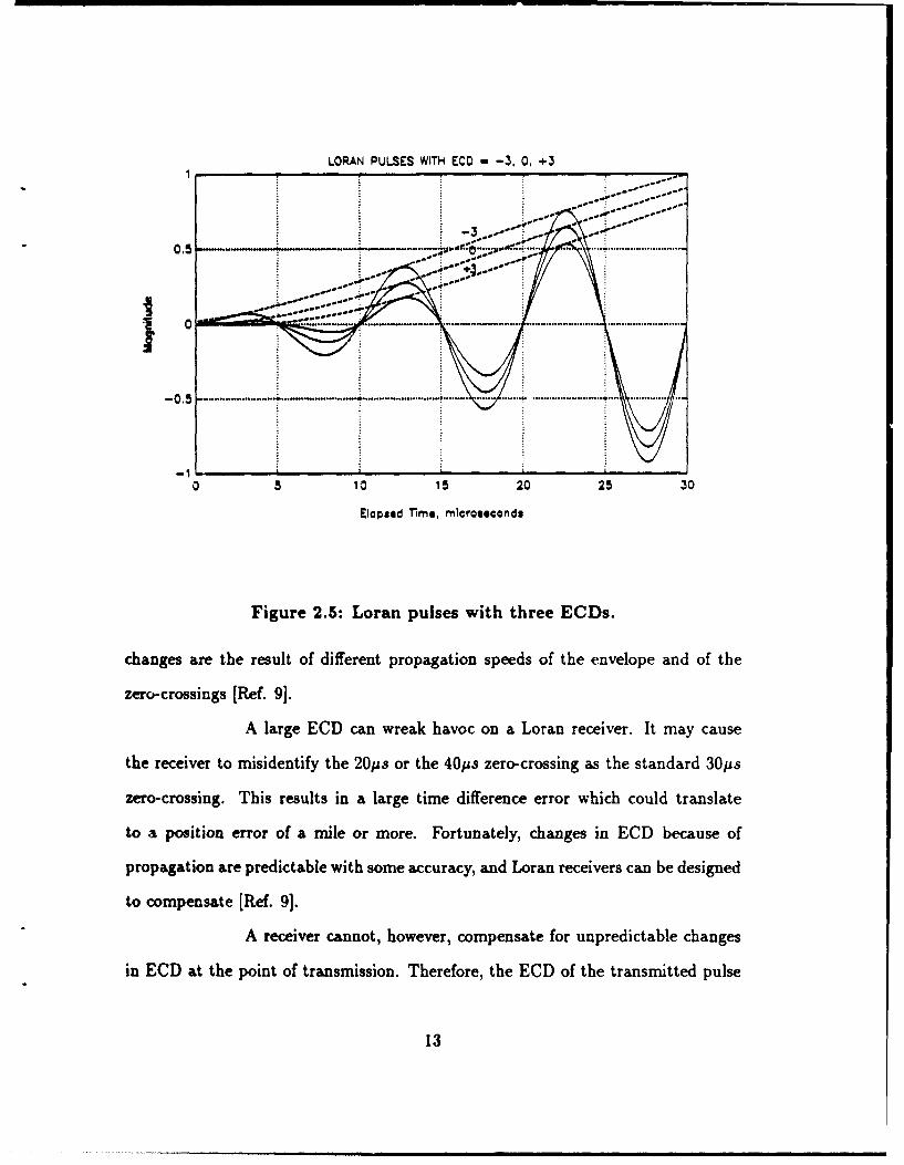
Test 1: Envelope-to-Cycle Difference (ECD). The Envelope-to-Cycle Dif-

ference is Ln indication of the position in time of the envelope of the Loran pulse

relative to the position of the zero-crossings. Figure 2.5 shows the first few half-

cycles of three Loran pulses with ECD values of -5, 0, and +5ps, respectively. A

negative ECD indicates that the envelope has been shifted left (or appeared earlier

in time) relative to the zero-crossings. A positive ECD indicates the opposite. The

ECD of the Loran pulse may be controlled arbitrarily, within specified limits, at the

transmitter to obtain a desired pulse shape.

One problem with ECD is that it changes as the pulse propagates.

First, when the Loran-C pulse is transmitted, a 900 carrier phase shift occurs by the

time the pulse has reached the far E-field [Ref. 1: p. 21], resulting in a change in the

ECD of +2.5ps. Second, depending on ground or ocean conductivity, ECD continues

to change as the pulse propagates over the earth's surface. One model predicts that

for every 100 Nm the pulse travels over the ocean ECD cLanges by -0. 2 5pu These

12

LORAN PULSES WITH ECD - -3, 0, +31 - . . .......... .

Fiur 25:Loanpuse wit three E s.."

A large • E can• wra ao na oaeevr.I aas

zeo-rosig Thi reulsin a lag tim difrneerrwic:olrnlt

to copesae Re.• 9.....

*- • I I

0 1 1 2 S -o

A lrgeeive cannt hwevr, hc ompnsat foraunpredcvrItmabl changse

i atthe reepe omisdntofy transmissin Thrfre the 40CD zeocossnf the stransmittd pulse

1 3

propagtion re preictabelwit d Tome, a icurascynd Lrnrcies a edsge

zeocrossingsat [Ref. 9].

the rceive toeisienifyter cnnorthoeer ompesazero-cossn asnthedistandar 3hangs

in ECD at the point of transmission. Therefore, the ECD of the transmitted pulse

13

is controlled carefully. Each station is assigned a local, or transmitted, ECD value,

usually zero. The station's actual transmitted ECD must differ by more than ±0.Sps

from the assigned transmitted ECD. This tolerance is just one sixth of the largest

ECD difference shown in Fig. 2.5.

Estimating the ECD of a Loran pulse is a complicated process, but it

can be done iteratively using the values of the first eight half-cycle peak amplitudes.

Appendix A outlines this procedure. Once the ECD of the transmitted pulse is

estimated, an ideal pulse with the same ECD may be generated according to Eq.

(2.1). The half-cycle peak amplitudes of this ideal pulse are used in the next two

tests, which apply only for transmitted ECD values of -2.5 to +2.5/ps.

Test 2: Half-cycle Peak Amplitudes (Ensemble Tolerance). The root-

mean-square (rms) error between the first eight actual half-cycle peak amplitudes

and first eight ideal half-cycle peak amplitudes must not be more than one percent

of the peak amplitude of the pulse. Specifically, let Sp, p = 1,2,... ,8, represent

the "ensemble" of the first eight half-cycle peak amplitudes of the actual antenna

current waveform, in amperes, normalized so the largest positive value of the entire

pulse (usually at, or near, half-cycle number 13) equals one. Let Ip, p = 1,2, -. , 8,

represent the ensemble of the first eight half-cycle peak amplitudes of the ideal

antenna current waveform, in amperes, normalized in the same way. Then,

8=I'8 < .01 (2.2)

Test 3: Half-cycle Peak Amplitudes (Individual Tolerances). In the first

eight half-cycles of the pulse, the largest difference between the ideal and actual

half-cycle peak amplitudes must not exceed three percent of the peak amplitude of

14

the pulse. In half-cycles 9 through 13, this requirement is relaxed to ten percent:

lIp - SjI _ .03 1 <p:ý,8 (2.3)

I4p-Spl _< .10 9_<p_513 (2.4)

Test 4: Zero-crossings. Loran transmitters are extremely narrowband ampli-

fiers designed to resonate at exactly 100.00 kHz. They are usually well tuned

to this frequency, but instantaneous frequency distortions may exist in the Loran

pulse, especially in the first two half-cycles. Since a Loran receiver depends heavily

on the time-domain behavior of the Loran pulse when sampling zero-crossings and

half-cycle peak amplitudes, any instantaneous frequency distortions in the pulse can

affect the performance of the receiver. A simple frequency domain spectrum analysis

of the entire Loran pulse may not adequately detect instantaneous frequency dis-

tortions in the pulse. Therefore, a time domain analysis of instantaneous frequency

covering the first 13 half-cycles of the pulse is used instead.

The zero-crossing times and tolerances in Table 2.4 have been estab-

lished for the Loran-C pulse [Ref. 1]. Category 1 tolerances are the most stringent

and are generally applied to the newer generations of transmitters. Category 2 toler-

ances are more lenient and are usually applied to the older transmitters. Reference

1 lists exactly which category applies in each test for every station in the Coast

Guard.

2. The Loran-C Pulse Group

a. Format of the Pulse Group

The Loran signal consists of a group of eight individual pulses trans-

mitted in rapid succession. This increases the average signal power available to the

receiver [Ref. 8: p. 33]. In addition to these eight pulses, the master station also

15

TABLE 2.1: ZERO-CROSSING TIMES AND TOLERANCES

Zero- Tolerance (ns)crossing (,us) Time (ps) Category I1 Category 2

5 -25 ±1000 ±200010 -20 100 150015 -15 75 100020 -10 50 50025 - 5 50 25030 standard (time reference)

zero-crossing35 5 50 10040 10 50 10045 15 50 10050 20 50 10055 25 50 10060 30 50 100

transmits a ninth pulse, which helps the receiver to identify the master. The ninth

pulse, when "blinked" ON and OFF according to a preset code, allows the master

station to notify a secondary station in the chain that the secondary is transmitting

a signal outside of specified tolerances. The Loran pulse decays essentially to zero

in 500ps; the pulses in the group are 1000 js apart, except that the master's ninth

pulse is transmitted 2 0 00 ps after its eighth pulse.

b. Multipulse Trigger

From the receiver's point of view, the standard zero-crossing pro-

vides the time reference for each pulse in the group and from group to group. From

the transmitter's point of view, the time reference is the Multipulse Trigger (MPT).

When it is time for a station to transmit a pulse group, the Loran timer equip-

ment sends 8 trigger signals, spaced 1000ps apart, to the pulse generator (PGEN)

16

(and one more trigger 20001is later in the case of the master station). When the

PGEN receives a trigger signal, it sends a transmitter drive waveform (TDW) to

the transmitter and a Loran pulse is produced and is radiated from the antenna.

When controlling the transmitted Loran signal, then, the MPT is used as the main

time reference point for the Loran signal. In this thesis, the standard zero crossing

is used only to perform the zero crossing test on an individual pulse.

c. Pulse Group Phase Coding

Another reason for the Loran-C pulse group is to distinguish the

Loran groundwave from Loran skywaves. As in other low-frequency systems, radio

waves may take multiple paths to reach a receiver. The groundwave follows the

surface of the earth while skywaves are refracted and reflected by the ionosphere to

return to the earth's surface. Generally the groundwave is used to calculate Loran

time differences. Therefore a skywave, which has traveled a longer path and is

thus delayed significantly, represents a spurious signal and may cause a large time

difference error if interpreted accidentally as the groundwave. To distinguish the

groundwave from skywaves, pulse group phase coding is used.

Phase coding is based on the fact that only the skywave undergoes

a change in phase when traveling from the transmitter to receiver. The ionosphere

refracts and reflects the pulses in the group and changes their phases by an arbitrary

amount. The groundwave's pulse group, on the other hand, arrives at the receiver

without a phase change (except for the 900 carrier phase shift from the near to

the far field, which affects all the pulses about equally). Phase coding shifts the

phases of certain pulses in the group by exactly 1800 at transmission, according to

a standard pattern shown in Table 2.2.

17

TABLE 2.2: LORAN-C PHASE CODES

Pulse StationGroup Master Secondary

A ++--+-+-+ +++++--+

B +--+++++- +-+-++--

A "+" indicates no phase change, and a "-" indicates a 1800 phase

change. Equipped with this expected pattern, the receiver successfully distinguishes

the groundwave from skywaves. Two successive pulse groups, A and B, are required

to implement this scheme. This two-GRI transmission sequence, called a Phase

Code Interval (PCI), repeats constantly.

d. Transmitter Power Supply Droop

When ei. ht or nine pulses are transmitted in rapid succession, the

transmitter's power supply may not recover fully from pulse to pulse. This problem,

most prevalent in older transmitters, causes the amplitude of each successive pulse

in the group to decrease. In general, the first pulse in the group is the largest and the

last pulse is the smallest. The decrease in amplitude of the smallest pulse relative to

the largest pulse is called the "droop" and is defined in percent. The Coast Guard

has established droop tolerances, which are included in the pulse group uniformity

tests described later in this subsection.

The practice of dual-rating, explained more fully in Subsection B.4.,

accentuates the droop. A dual-rated station, located between two contiguous Loran

chains, transmits pulse groups for two chains. Since the power supply of a dual-rated

18

station often has less time to recover than that of a single-rated station, dual-rated

stations are given larger tolerances for droop.

e. Specification: Uniformity of Pulses Within a Group(Three Tests)

Of the four tests applied to the individual Loran pulse, and ex-

plained earlier in Subsection B.1.(b), the tests of the half-cycle peak amplitudes

(ensemble tolerance), the half-cycle peak amplitudes (individual tolerance) and the

zero-crossings are applied only to pulse one. To measure uniformity of the pulses

within the group, the test of ECD (as described in Subsection B.1.) is applied to

each pulse. Two more tests, which examine pulse-to-pulse amplitude differences and

pulse-to-pulse timing differences, are also applied.

Test 1: Pulse-to-Pulse ECD Differences. This test reflects in a general way

how the shape of one pulse differs from the shapes of the others in the group. The

ECD of any single pulse must not differ from the average ECD of all the pulses in

the group by more than the tolerances in Table 2.3.

TABLE 2.3: PULSE-TO-PULSE ECD TOLERANCES

I Category 1 Category 2

Single-rate 0.5ps 1.OsS

Dual-rate 0 .7 ps 1 .5ps

Test 2: Pulse-to-Pulse Amplitude Differences. The amplitude of the small-

est pulse in a group must not differ from the amplitude of the largest pulse in that

group by more than the limits in Table 2.4, calculated as follows:

19

TABLE 2.4: PULSE-TO-PULSE AMPLITUDE TOLERANCES, ORPERCENT DROOP (D)

Category IJ Category 2

Single-rate 5% 10%

Dual-rate 10% 20%

D = Ipk max -Ip, min X 100 (2.5)Ipk max

where

Ip4 max is the value of i(t) at the peak of the largest pulseIpk Min is the value of i(t) at the peak of the smallest pulse

Test 3: Pulse-to-Pulse Timing Differences. Pulses two through eight are

transmitted at consecutive integer multiples of 1000js after pulse one. Relative to

the standard zero-crossings of pulse one, the standard zero-crossings of pulses two

through eight must meet the tolerances listed in Table 2.5.

Pulse nine, which follows pulse 8 by 2000iss in the master pulse

group only, is used mainly to identify the master signal and is not used for navigation

[Ref. 1: p. 2-9]. Thus a tolerance is not assigned to its position in time.

3. Blink and "Out-of-tolerance"

Whenever a baseline is not useable for navigation, the first two pulses of

that secondary station's pulse group are "blinked" ON and OFF repeatedly (0.25

seconds on, 3.75 seconds off). The Loran receiver passes along this warning to the

user, often actually blinking ON and OFF the time difference reading on its display

20

TABLE 2.5: PULSE-TO-PULSE TIMING TOLERANCES

[ Category 1 Category 2

Single-rate (p - 1)1000ps ± 25ns (p - 1)1O000s = 50ns + C

Dual-:ate (p - 1)1000s ± 50ns (p - 1)1000ps - lOOns + C

Note: p is the pulse number (2 through 8) of the pulses which follow the first pulse within eachgroup. C is 0 for positively phase coded pulses; ICI < 150ns for negatively phase codedpulses. The standard zero-crossing of pulse one is the time reference within each group.

panel. The transmitter station or the control station initiates blink for any of the

following reasons [Ref. 1: p. 2-8]:

* Time difference out of tolerance,

* ECD out of tolerance,

* Improper phase code or GRI, or

e Master or secondary station operating at less than one half of specified output

power, or master station off air (not transmitting a signal at all).

Automatic alarms at the transmitter station and the control station sound when

these quantities are out of tolerance.

In the definition of blink, the four tests of pulse number one and the three

tests of the entire pulse group explained above are conspicuously absent. There are

at least two reasons for this. The first is that the control station, with its Loran

receivers, is monitoring the most important aspects of the Loran signal as far as

the user is concerned: it ensures that a receiver can maintain lock and that the

time difference is correct. In this sense, the fine details of the pulse which are the

21

subject of these seven tests go beyond the minimum requirements of the Loran

system to keep a useable baseline. The second reason is that most of the Loran

control equipment suite was designed and built before modern signal processing

equipment was available, and consequently these demanding tests are not conducted

continuously either at the transmitting station or control station.

Instead, during a one-hour period each day designated for "system sam-

ple," an operator at each transmitter station manually tests ECD, the half-cycle

peak amplitudes (ensemble tolerance), and the half-cycle peak amplitudes (individ-

ual tolerance), using an oscilloscope to measure the pulse peaks. He or she then

enters the values by hand into a computer, which performs the tests and records

the results. If a failed test is not accompanied by one of the conditions requiring

blink, station personnel usually do not initiate blink, but instead interpret the test

as an indication that transmitter maintenance is needed. From time to time, station

personnel perform all seven tests and several more as well using a portable Loran

Data Acquisition (LORDAC) unit. They use these results to keep the transmitter

operating properly, but generally do not initiate blink if a test fails.

These seven tests thus represent a stricter standard than the conditions

requiring blink and serve as an early warning of possible transmitter system problems

which may later require blink. Therefore, a pulse out of tolerance in one of these

seven tests may still be useable for navigation, but this is not a desired condition.

4. Dual-rating and Dual-rate Blanking

As mentioned briefly before, a dual-rated station, located between two

contiguous chains, transmits pulse groups for two chains. These chains always have

different GRIs, or rates. Since each chain is independently controlled, dual-rated

stations are subject to competing, and sometimes conflicting, requirements as the

pulse groups from the two GRIs periodically overlap in time. Since it is undesirable

22

to transmit part of one pulse group and part of another, the conflict is solved by

transmitting one and suppressing, or "blanking," the other. Blanking, which relates

to the synchronization of two rates, should not be confused with blink, an indication

of an out-of-tolerance condition.

Implementing dual-rate blanking is straightforward. A dual-rated tube

transmitting station's timing equipment sets up a blanking interval over each pulse

group, beginning 5001ts before the first pulse is triggered and ending 140011s after

the last pulse is triggered. The timing equipment tracks the two blanking intervals

as they move in time. When they overlap, the timer sends MPTs for only one of

the two rates to the PGEN.

Two methods are used to decide which rate is blanked when an overlap

occurs. In priority blanking, the same rate is always blanked, generally the shorter

one. In alternate blanking, the priority role is passed back and forth between the

rates at a time interval equal to the length of four times the longer GRI [Ref. 1: p.

2-9].

5. Frequency Spectrum Requirements

The energy that a station transmits outside the assigned 90 to 110 kHz

band must not exceed one percent of total radiated energy. Furthermore, neither

the energy below 90 kHz nor the energy above 110 kHz may exceed 0.5% of total

radiated energy.

C. PRODUCING THE SIGNAL

1. The Loran Transmitter

a. Types of Transmitters

As mentioned previously, Loran-C transmitters are extremely nar-

rowband amplifiers designed to resonate at exactly 100.00 kHz. The Coast Guard

23

currently operates four types of transmitters, as listed in Table 2.6. The three types

of transmitters with vacuum-tube power amplifier stages represent three generations

of tube transmitter technology. The fourth generation, the solid-state transmitter,

is now the state-of-the-art in Loran-C.

The solid-state transmitter is superior to the vacuum tube transmit-

ter: it has a cleaner output signal, it has a higher ratio of output power to supplied

line power, it is more robust, and it requires less maintenance than any other trans-

mitter type. It also has an automatic pulse generating and control system. Many of

the stations equipped with this transmitter are unmanned and remotely operated.

For all these reasons, the Coast Guard has considered replacing all of

its older transmitters with the solid-state transmitter. However, the relatively high

replacement cost ($2 million to $4 million per station) and the impending closure of

some tube stations have kept the tube transmitters in operation for the foreseeable

future. When the last AN/FPN-39 transmitters are removed from service in the next

year or two, the only tube transmitter classes remaining will be the AN/FPN-42

and the AN/FPN-44/44A/44B/45. The '44 variants and the '45 are essentially the

same transmitter with progressively more power amplifier stages and consequently

greater output power. The '42 and the '44A, the subjects of this report, adequately

represent the remaining tube transmitters.

b. Transmitter Loads

Each station has two different transmitter loads: the antenna and

the resistive dummy load. Several types of antennas are in service, and they vary

in radiated power and range. The two most common types are the 625-ft and the

700-ft top-loaded monopoles. The radiating part of these antennas consists of a

single steel tower and an umbrella-like cap of guy wires leading from the top of

24

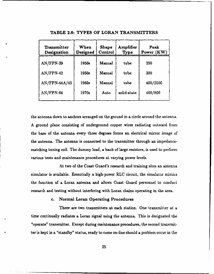
TABLE 2.6: TYPES OF LORAN TRANSMITTERS

Transmitter When Shape Amplifier PeakDesignation Designed Control Type Power (KW)

AN/FPN-39 1950s Manual tube 250

AN/FPN-42 1950s Manual tube 300

AN/FPN-44A/45 1960s Manual tube 400/2000

AN/FPN-64 1970s Auto solid-state 400/800

the antenna down to anchors arranged on the ground in a circle around the antenna.

A ground plane consisting of underground copper wires radiating outward from

the base of the antenna every three degrees forms an electrical mirror image of

the antenna. The antenna is connected to the transmitter through an impedance-

matching tuning coil. The dummy load, a bank of large resistors, is used to perform

various tests and maintenance procedures at varying power levels.

At two of the Coast Guard's research and training sites an antenna

simulator is available. Essentially a high-power RLC circuit, the simulator mimics

the function of a Loran antenna and allows Coast Guard personnel to conduct

research and testing without interfering with Loran chains operating in the area.

c. Normal Loran Operating Procedures

There are two transmitters at each station. One transmitter at a

time continually radiates a Loran signal using the antenna. This is designated the

"operate" transmitter. Except during maintenance procedures, the second transmit-

ter is kept in a "standby" status, ready to come on-line should a problem occur in the

25

operate transmitter. Periodically the stanaoy and operate designations are switched,

allowing technicians to perform maintenance on the formerly ope'rate transmitter.

The standby transmitter may send pulses into the dummy load at any time with-

out disturbing the operate transmitter and its signals. When transmitter switches

interrupt Loran-C service for less than one minute, the Coast Guard considers the

station to be transmitting continuously for availability recording purposes.

d. Nonlinear and Time-Varying Behavior of TubeTransmitters

This thesis incorporates two important assumptions. First, Loran

tube transmitters are nonlinear devices, but behave linearly at a given operating

point. This assumption is examined and supported in detail in the next chapter.

Second, the transfer functions of the tube transmitters also vary with time. As

transmitter components, particularly the vacuum tubes in the amplifier sections,

age over days and weeks, their amplifying characteristics change. When components

are Leplaced, small step changes occur to the transmitter's transfer function. When

the operate and standby transmitters are switched, the pulse shape control system

encounters a larger step change in the plant's transfer function. Loran technicians

minimize these effects by a great deal of hard work, but the effects still exist to some

degree. In addition to these internal factors, weather conditions, such as ice forming

on the antenna and high winds (which distort the shape of the antenna slightly)

introduce other time variations as well. Thus, from the point of view of a Loran-C

control system, the transfer function of this plant exhibits both blow changes and

periodic step changes over hours, days and weeks. In the absence of severe weather

conditions or component failure, the transmitter may be considered time invariant

for a period of several hours. This assumption is used also in the next chapter.

26

e. Transmitter Phase Code Balance

Tube transmitters use a push-pull amplification system, where the

positive and negative parts of each pulse are amplified by separate banks of tube

amplifiers. If the transmitter is not balanced properly, the positive half of the signal

will be amplified more than the negative half, or vice versa. Most often this is

detected when examining pulses whose phase code is different in GRIs A and B.

When the pulse flips back and forth, it appears to "bounce." Phase code balance

is an adjustment built into the PGEN which increases the magnitude of the TDW

for negatively phase coded pulses (those pulses which have been inverted by a 1800

phase change). In this way the phase code "bounce" is removed.

2. Transmitter Drive Waveforms and Typical Outputs

A cosine pulse input is used to excite the highly resonant Loran trans-

mitter. A typical TDW and radio frequency (RF) antenna current waveform are

shown for both the '42 and the '44A. The terms input and input waveform refer

to the TDW, and the terms output and output waveform refer to the RF pulse

captured at the transmitter ground return. Actually both input and output are at

the same radio frequency.

In both TDWs, the cosine pulse includes eight full periods or, by Loran

convention, sixteen half-cycles. To meet spectrum requirements on the '44A, a "tail

drive" circuit adds a damped sinusoid to the end of the input cosine pulse to slow

the decay of the RF output pulse. This prevents unwanted frequency components

from appearing in the output. When input half-cycle 16 equals zero, as in Fig. 2.7,

the tail drive is suppressed.

27

3. Controlling the Pulse Shape

In Figs. 2.6 and 2.7, each input half-cycle has a different peak ampli-

tude. This is the result of the manual control scheme designed for the vacuum tube

transmitters in the 1950s and 1960s and the pulse generator (PGEN) which imple-

ments it. By turning one of the 16 dials on the face of the pulse generator, the peak

amplitude of any of the 16 input half-cycles may be adjusted in ten discrete steps.

The controls of the two PGENs are shown in Fig. 2.8.

By observing the full-wave rectified RF pulse overlaid with the envelope

of the ideal pulse, the dials of the PGEN may be adjusted to match the actual RF

pulse shape to the ideal. The manual control system used for pulse shaping in the

tube transmitters is diagrammed in Fig. 2.9.

The manual process of "pulse building" on a tube transmitter is one of

the most difficult tasks in Loran-C system operation. Adjusting one half-cycle of

the input affects not just one half-cycle of the output but all of the pulse which

follows it in time. Also, the discrete steps available on the PGEN may result in

large jumps in the amplitudes of the output pulse's half-cycle peaks. Added to this

are the nonlinearities of the tube transmitters. Even with skilled and experienced

operators this process can take several hours. Fortunately, time variations in the

transmitter's operating characteristics ordinarily change even more slowly, so when

pulse building, time variations may be ignored. However, because of these slow

time variations, on each occasion when pulse-building is attempted, the transmitter's

operating characteristics are slightly different. From one point of view, this amounts

to manually controlling in a sixteen-dimensional space a nonlinear device which

behaves slightly differently each time the control procedure is attempted.

28

TDW: AN/FPN-42 TRANSMITTER

0.5 - -------- --......................................

-05 .--••. ...--.............

-- 1 .' .

-1.5- - J0 50 100 150 200 250 300 350 400 450

Time, microseconds

RF PULSE: AN/FPN-42 TRANSMITTER

-1.5 ...

-0.5 i . . , . . . .. .. ... ............. .................. i..................

0 50 100 150 200 250 300 350 400 450

Time, microseconds

Figure 2.6: '42 input and output, antenna simulator, pair 30.

29

"'' ~ ~ ~ ~ ~ ~ ~ ~ ~ ~ ~ ~ m "immlmlmnnlnlllmlI

TDW: AN/FPN-44A TRANSMITTER

0. - - r' i" •

0.5 -

0.5

-1.5 . .... ..... .

0 50 100 150 200 250 300 350 400 450

Time, microseconds

RF PULSE: AN/FPN-44A TRANSMITTER

0.5 ........ .............. ...........

0.5 ... ..............

-16----I-A 80 50 100 150 200 250 300 350 400 450

rime, microseconds

Figure 2.7: '44A input and output, antenna simulator, pair 72.

30

Figure 2.8: Two pulse generators.

TDW PULS10XMTR PUS

PGENSCP

TIMER IDEALPULSE

Figure 2.9: Manual control diagram.

31

Understandably, many technicians have opted to control the pulse from

the "back end" by keeping the transmitter tuned identically at all times instead of

attempting to compensate for time variations in the transmitter using the PGEN.

While the results are often more predictable, this approach is certainly time inten-

sive. Although an automatic pulse generation and control system was designed for

the solid-state transmitter, none has yet been implemented for the tube transmitters.

D. THE ELECTRONIC EQUIPMENT REPLACEMENTPROJECT (EERP) AND THE PURPOSE OF THISRESEARCH

1. The EERP and its Plan 1

In answer to the difficulties of manually controlling a tube transmit-

ter and in response to many other considerations beyond the scope of this paper,

in 1990 the Commandant of the U.S. Coast Guard assigned to the Coast Guard

Electronics Engineering Center (EECEN) a multi-year project titled the Electronics

Equipment Replacement Project [Ref. 7]. In identifying portions of the Loran-C

system requiring a redesign effort, EECEN considered the following:

* The supportability of current and future equipment,

* The'desire to enhance and expand automation,

9 The need to respond to new system requirements, and

* The desire to remain in close step with technology.

This process resulted in five major plans. Plan One, titled "EPA/PGEN/-

LORDAC Redesign," calls for a redesign of the entire tube transmitter's monitor

and control equipment suite, including the Electrical Pulse Analyzer (EPA) and the

Loran Data Acquisition (LORDAC) equipment. The new control system should be

32

able to monitor and analyze the Loran pulse continuously, or nearly continuously;

generate and control a Loran-C pulse in tolerance automatically; and record the

results necessary to build a database of operational history [Ref. 7].

2. The VXIbus Based Loran-C Transmitter and Control System

In 1990 EECEN began to implement Plan One of the EERP by starting

project W1180, originally titled "EPA/DPA Redesign" and subsequently renamed

"Timing and Control Equipment (TCE) Redesign." In a 1991 report titled "The

VXIbus Based Loran-C Transmitter and Control System," Taggart and Turban

describe a prototype control system constructed at EECEN which, it is hoped, will

perform these functions [Ref. 10]. A simplified diagram of this control system is

shown in Fig. 2.10.

The system works as follows: The computer loads an initial TDW into

an arbitrary function generator (AFG), which sends the TDW to the transmitter at

each timer trigger. A digital storage oscilloscope (DSO) samples the RF pulse and

stores it in the computer's memory. In a closed-loop fashion, the controller then

computes a new TDW in an attempt to reduce the error between the actual and

ideal RF pulses.

Based on the new generation of Automatic Test Equipment known as

VMEbus Extensions for Instrumentation (VXlbus), this system will be much smaller

and will have fewer components than the equipment used today. It will give the

operator new control capabilities over each pulse in the pulse group. This system

will thus produce a more consistent Loran signal while reducing maintenance.

Even though the '42 transmitter is not included in the EERP (it will be

phased out in the next few years), it is simpler to operate than the '44A and will

be valuable when developing this VXIbus system. In the end, the VXIbus control

33

TDW XMTR PULSE T

CPU / DSO

STIMER ,•IDEAL

PULSE

Figure 2.10: Diagram of the VXIbus based control system.

system will operate with the '44A but not with the '42 [Ref. 7, 10]. For these

reasons, both the '42 and the '44A are included in this research.

3. Purpose of This Research

a. Primary goal: A Control Algorithm

One of the missing pieces in this VXIbus system is a proven al-

gorithm to generate and control the Loran-C pulse shape automatically. Finding,

developing and testing such an algorithm is the primary goal of this research. This

paper contributes directly to Phase II of project Wi180, Pulse Generator Redesign

[Ref. 11]. The other phases of Project W1180 are specifically excluded from this

paper except where they overlap with Phase II. Furthermore, within Phase II, only

34

the pulse-shaping aspects of the PGEN redesign are considered. Precision timing

between pulses and pulse groups is excluded.

b. Necessary Tool: A Computer Simulation Program

Achieving this goal requires a detailed computer program to sim-

ulate the operation of the '42 and '44A tube transmitters and those parts of the

VXIbus control system involved in pulse shaping. There are at least three reasons

for this. First, testing new types of transmitter drive waveforms, especially in closed

loop control, is safer on a computer than on a 400 kilowatt transmitter. Second,

working with a computer simulation is much faster, much easier and much more

convenient both for the researchers in Monterey, California and for the EECEN

technicians in Wildwood, New Jersey. Third, in this simulation the researcher con-

trols the transmitter completely and can isolate the effects of different transmitter

and control system factors on an algorithm. In this way control algorithms may

be tested more thoroughly in simulation than with an actual transmitter. In the

next chapter, mathematical models for the '42 and '44A are developed to use in the

simulation program.

35

[THIS PAGE INTENTIONALLY LEFT BLANK]

36

III. MODELING THE AN/FPN-42 AND 44ALORAN-C TRANSMITTERS

A. INTRODUCTION

Simulating a dynamic physical system requires a dynamic model, a mathe-

matical representation which transforms an input signal into an output signal just as

the real system does, under the normal range of operating conditions. In this chap-

ter, explicit mathematical models for the AN/FPN-42 and AN/FPN-44A transmit-

ters are developed and tested. First, the modeling approach and data are described.

Second, the unit sample response of the '42 transmitter is identified. Third, a lin-

ear, time invariant (LTI) pole-zero model is developed for the '42; next, observed

nonlinearities and time variations are added to the model. After the performance

of this model is tested, the entire process is repeated for the '44A.

B. THE MODELING APPROACH

1. Discrete-Time Representation

A discrete-time model represents the transmitters in this research, for

several reasons. First, the VXIbus is a discrete-time system, and discrete-time

techniques are most easily transferable to it. Second, this field is well-developed in

the signal processing literature. Third, working with a discrete-time model is most

convenient. The data is in discrete-time form already and many useful discrete

signal processing algorithms and computer programs are available.

37

2. Data from the '42 and '44A transmitters

a. Data Collection

EECEN provided eighty-six discrete-time input and output data

sequence pairs for this project, sixty-seven pairs for the '42 and nineteen for the

'44A. For twenty-seven of these the dummy load was connected to the transmitter

instead of the antenna or the antenna simulator. Sampled at 10 MHz by a LeCroix

9410 digital oscilloscope with eight bits of resolution, each sequence is 4096 points in

length and covers a time period of 409.6 ps. The input sequence, which is the TDW,

and the output sequence, which is the RF pulse, were sampled simultaneously on

channels A and B of the oscilloscope. The two signals are synchronized to within

100 ns, the length of time between adjacent samples.

The RF pulses were measured at the ground return line to the trans-

mitter using a Pearson current transformer. Both the TDW and the RF data se-

quences were measured in volts, with the input impedance of the oscilloscope set

to infinity. Accordingly, this simulation uses volts for both TDW and RF pulse.

Although the RF pulse is customarily measured in amperes, this difference is only

a scaling factor and does not affect the validity of the simulation.

These data sequences are essentially the same as those available on

the VXIbus system, which uses an eight-bit Tektronix digital storage oscilloscope.

This similarity strengthens the usefulness of this simulation since a control algorithm

has nearly identical data to work with in this program as well as in the VXIbus

system.

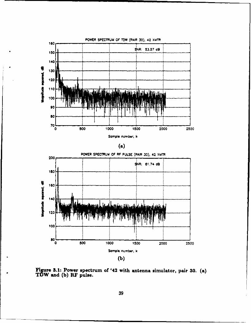
b. Effects of Noise and Quantization

Figures 3.1a and 3.1b show the power spectra of the above two se-

quences. Figure 3.1c is a closeup of this plot. These are the periodogram estimates

38

POWER SPECTRUM O TOW (PAIR 30), 42 XMTR160

SNR: 53.57 d8IS 0 •.4-• .*. . . .. ........ ... ........ ....................... ........

*130

120-

t 110'

100" --- .... .........

700 500 1000 1500 2000 2500

Sample number, k

(a)POWER SPECTRUM OF RF PULSE (PAIR 30), 42 XMTR

200

SNR: 61.74 d8

IGO-.. . . . . .......-- .. ... ... ... ............. ...............................

120

10 0 -- ... . ...... . . .. ..

0 500 1000 1500 2000 2500

Sample number, k

(b)

Figure 3.1: Power spectrum of '42 with antenna simulator, pair 30. (a)TDW and (b) RF pulse.

39

CLOSEUP: POWER SPECTRUM OF TOW & RF (PAIR 30), 47 XMTR190

17025 " 3 0 4 0 5 6

Sapl numbr,:

Fiue3l: Cloeu of poe pcrm '4,, pi 0

1300\oo

130 ... .• .... . ----.

1 1 0 ---------

23 30 35 4.0 45 so 55 60

Sample number, k

Figure 3.1c: Closeup of power spectrum, '42, pair 30.

expressed in decibels [Ref. 12, p. 448]. Sample 41 corresponds to 100 kHz and

sample 2049 corresponds to 5.00 MHz, one half the sample frequency. Figure 3.1c

also marks the 90-110 kHz frequency band of Loran-C.

The transmitter's behavior as a highly narrowband amplifier is ap-

parent in these figures. In this data pair the signal-to-noise ratio (SNR) increases

from 51 dB to 61 dB from input to output. Here the SNR is defined in decibels as the

peak signal value minus the average value of the noise found in the highest twenty

percent of the frequency range of the power spectrum. Underlying this definition are

the assumptions that the Loran signal power present in this upper frequency band is

negligible compared to the noise power and that the noise is white or approximately

40

white. Some of the noise that appears in the output is inherent in the transmitter

system itself, and some is quantization noise added by the sampling oscilloscope.

Chapter V includes comparison results when each is varied.

3. Linearity and Time Invariance

a. Initial Assumption: Linear, Time Invariant (LTI) WithinEach Pulse

In this work, a fundamental assumption was made that the tube

transmitters behave as linear, time invariant (LTI) systems at a given operating

point, within a limited time interval [Ref. 13, 141.

b. Verifying the Assumption

Testing a system for linearity and time invariance with all possible

input sequences would be impossible. However, if the assumption is made that a

system is LTI under certain operating conditions, its behavior may be completely

represented by a unit sample response sequence, h(n), the discrete version of the

impulse response. Then the system output can be represented as a linear convolu-

tion,

y(n) = x z(m)h(n - m) = x(n) * h(n), (3.1)M-00

where z(n) is the input sequence. With its shifting, multiplying and summing op-

erations, linear convolution tests the crucial properties of LTI systems [Ref. 12, pp.

24-25, 1031. A good match between a "synthetic" output sequence y.(n) (produced

by convolving actual input x(n) with the proposed h(n)) and ihe actual output

sequence y(n) strongly implies that the assumption of LTI behavior is valid. From

this point, an analysis of the system may proceed using mathematical techniques

applicable only to LTI systems, subject to further validations as more data becomes

available or the operating point changes.

41

From an analysis of the data pairs available, the operating point is

assumed to be a function of the shape of the TDW. If this remains unchanged from

pulse to pulse, the operating point and the unit sample response also stay the same.

As explained in the last chapter, the limited time interval in which this assumption

is considered valid is a period of several hours.

The '42 model is developed first for a typical operating point before

examining other operating points. The TDW and RF pulse shown in Fig. 2.6 define

this typical operating point. The shape of this TDW, including the 80 Ps length

of the significant part, is representative of the TDWs used in operating the '42

transmitters in the Coast Guard.

Analysis revealed that the '42 transmitter no longer behaves linearly

when TDWs are applied which excite the transmitter longer than 90 Ps. This

is apparent in the frequency domain. By linear theory, the bandwidth of an RF

pulse should be no wider than the bandwidth of the input. However, the RF pulse

bandwidth remained the same when the input signal bandwidth narrowed, and a

linear model could not be constructed. Therefore, for TDWs in this category, this

modeling approach is inaccurate and should not be used.

c. Adapting the Assumption to Nonlinear and Time-VaryingBehavior

Implicit in the assumption above is the idea that when the shape

of the TDW changes, a different unit sample response may be required to represent

the transmitter accurately. Catenating a number of LTI models to cover a range of

operating points implements this idea. If the transmitter's operating points can be

identified with sufficient precision, and if a unit sample response sequence can be

identified for each one, then a system which is non-LTI overall may still be treated

as LTI.

42

4. Time-Domain Pole- Zero Modeling

a. Single LTI System

Each unit sample response sequence is by itself a useful mathemati-

cal model of the transmitter. Because each has a finite length, they may be classified

as finite impulse response (FIR) systems. Modeling an FIR system as an infinite

impulse response (IIR) system is often more efficient, because there are less param-

eters,. It is also more useful, because the roots of the IIR parameters have physical

significance. This is the approach used here.

An IIR system may be represented by a constant-coefficient differ-

ence equation of the form

y(n)+aiy(n-l)+...+apy(n-P) = box(n)+blx(n-1)+...+bQx(n-Q), (3.2)

or

aTy = bTx, (3.3)

where y(n) represents the output sequence and x(n) represents the input sequence.

Coefficients a,,--' , ap and bl,' ", bQ are real and constant. Taking the z-transform

of Eq. (3.2) yields the transfer function

H(z) - bo + baz-1 + ... + bQz-Q (3.4)1 + alz-1 + ... + apz-p "

Factoring the numerator and denominator of this rational polynomial produces the

alternate form

H(z) = bozpQ (z - f)(z f2)'". (z - fM)(z - g1)(z -92)" (z - gp)

where numerator roots fl," ', fQ are the zeros of the transfer function and denom-

inator roots .q, --',gp are the poles of the transfer function. Complex pole pairs

represent the natural or resonant frequencies of the system while zeros represent the

system's delays, gains, losses and initial conditions [Ref. 15, p. 3].

43

Pole-zero modeling in the time domain, as used in this thesis, is the

process of estimating the poles and zeros of an IIR system based on the least squares

criterion. The a coefficients are also known as the Autoregressive (AR) parameters,

and the b coefficients are also called the Moving Average (MA) parameters. Thus,

ARMA modeling is another term for pole-zero modeling, which uses both a and b.

Pole-zero modeling is characteristically applied to random processes

[Ref. 16]. Most of these sequences represent systems with underlying dynamics of

a relatively low order, overlaid by random noise. As Section C of this chapter

describes, the random noise is expressly filtered out to isolate the system dynamics

of the transmitter. These dynamics, not the random noise, are what the pole-zero

model is intended to capture.

b. Catenated LTI Models

Each model in the catenation may have a slightly different unit sam-

ple response sequence, but each is still an LTI model. Therefore, the catenated model

may be expressed as a linear difference equation with non-constant coefficients, of

the form

y(n) + ai(t, E.)y(n - 1) +-.. + ap(t, E,,)y(n - P)

=bo(t, E,)x(n) + bl(t, En)z(n - 1) + ... + bQ(t, En)x(n - Q), (3.6)

where each coefficient is a function of time, t, and of parameter E,,, which accounts

for the nonlinear behavior of the transmitter at different operating points and is

defined in Section E of this chapter. Both n and t are integer indices of discrete

time, but they are used differently. Index n, a multiple of the uniform 100 ns

sampling interval (for N = 1), appears in equations which represent transmitter

dynamics within a period of 409.6 ps. This period is too short to experience the

time variations described in the last chapter. Index t, on the other hand, represents

44

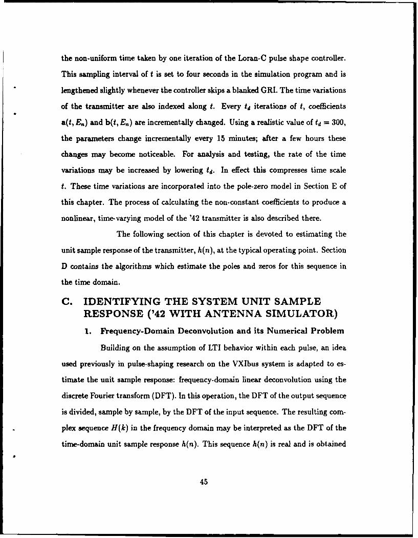
the non-uniform time taken by one iteration of the Loran-C pulse shape controller.

This sampling interval of t is set to four seconds in the simulation program and is

lengthened slightly whenever the controller skips a blanked GRI. The time variations

of the transmitter are also indexed along t. Every td iterations of t, coefficients

a(t, E.) and b(t, E.) are incrementally changed. Using a realistic value of td = 300,

the parameters change incrementally every 15 minutes; after a few hours these

changes may become noticeable. For analysis and testing, the rate of the time

variations may be increased by lowering td. In effect this compresses time scale

t. These time variations are incorporated into the pole-zero model in Section E of

this chapter. The process of calculating the non-constant coefficients to produce a

nonlinear, time-varying model of the '42 transmitter is also described there.

The following section of this chapter is devoted to estimating the

unit sample response of the transmitter, h(n), at the typical operating point. Section

D contains the algorithms which estimate the poles and zeros for this sequence in

the time domain.

C. IDENTIFYING THE SYSTEM UNIT SAMPLERESPONSE ('42 WITH ANTENNA SIMULATOR)

1. Frequency-Domain Deconvolution and its Numerical Problem

Building on the assumption of LTI behavior within each pulse, an idea

used previously in pulse-shaping research on the VXIbus system is adapted to es-

timate the unit sample response: frequency-domain linear deconvolution using the

discrete Fourier transform (DFT). In this operation, the DFT of the output sequence

is divided, sample by sample, by the DFT of the input sequence. The resulting com-

plex sequence H(k) in the frequency domain may be interpreted as the DFT of the

time-domain unit sample response h(n). This sequence h(n) is real and is obtained

45

directly from H(k) using the inverse DFT (IDFT). The fast Fourier transform (FFT)

speeds the computation of the DFT greatly.

One significant problem exists with this approach: spurious peaks in the

frequency domain, caused when output DFT samples are divided by input DFT

samples close to zero. An ideal filter eliminates most of this numerical noise by

setting equal to zero the elements of H(k) corresponding to frequencies less than

50 kHz (sample 40) and greater than 150 kHz (sample 123). Because the sequences

have been zero-padded to twice their original lengths, sample 82 now represents 100

kHz. However, spurious peaks still exist in the 50-150 kHz frequency band, as Fig.

3.2 demonstrates. These spurious peaks distort h(n) significantly; unfortunately,

zeroing frequencies in this range also distorts h(n). A more sophisticated filter is

required here.

2. Removing Spurious Peaks with Median Smoothing

A nonlinear smoothing technique consisting of running medians and a

lowpass linear filter can remove the spurious peaks in H(k) [Ref. 17]. First, the

signal is considered to be the sum of rough and smooth parts R[H(k)] and S[H(k)]:

H(k) = R[H(k)] + S[H(k)]. (3.7)

The running median Mu[H(k)], simply the median of the U-point sequence H(k -

M + 1),..., H(k - 1), H(k), H(k + 1),...,H(k + M - 1), replaces sample H(k).

Here U is an odd integer and M = (U + 1)/2. This smoother separates the rough

and smooth parts of the signal by removing single bamples with large errors. The

smoother's output effectively follows a low-order polynomial curve without distort-

ing the surrounding samples as a linear filter would [Ref. 17, p. 158]. This smoother

preserves sharp discontinuities, a property useful in many applications.

46

MAGNMUIJO OF* H(N) (PAIR 30)70 YF

I : --..- 4-. -.-...... . -. ................

20 - - '

40 so 60 70 s0 90 100 110 120 1.30

Sample number, k

(a)

PNASE OF H(N) (PAIR 30) ___

2A

-0 . ... ................ *"*-. . . ***....

-........................

Sample numnber. k

(b)

Figure 3.2: H(n) for '42 with antenna, pair 30, with antenna simulator.(a) Magnitude and (b) phase.

47

Often, however, a linear filter is used in combination with the median smoother to

soften these discontinuities. Here a succession of a five-point median smoother, a

three-point median smoother and a three-point lowpass hanning filter is used. The

hanning filter has unit sample response

h(n) = 1/4, n 0

1/2, n= 1

1/4, n -2. (3.8)

This combination smoother is applied twice each to the parts of H(k) corresponding

to frequencies 50-90 kHz (samples 41-74) and 110-150 kHz (samples 91-122). The

smoother is not used in the Loran frequency band, 90-110 kHz, since no spurious

peaks were observed in this band.

This approach proved to be quite effective, as Fig. 3.3 demonstrates.

The presence of more than one sharp discontinuity within U points can reduce the

effectiveness of this technique, as samples 114-118 of the phase plots demonstrate.

The estimated unit sample response, which appears in Fig. 3.4a, represents the

relatively low-order system dynamics virtually free of random noise and of the nu-

merical errors inherent in the frequency-domain deconvolution technique. This h(n)

is tested using linear convolution as before, with another similar input and out-

put data sequence pair. Figure 3.4b shows that the estimated sequence correctly

represents not only the resonances of the transmitter but also the amplitude and

phase.

Simulation tests using h(n) from both filtered and unfiltered H(k) show

that in the absence of spurious peaks in the 50-150 kHz band, the entire filtering op-

eration increases the mean squared error (MLE) between the synthetic pulse and the

48

MAGNITUJDE OF H.(N), SMOOTHED (PAIR 30)

..... .v

I* --- ------ --- ------------ - ----- ..........

40 50 so 70 80 90 10 10 120 130

Sample number, k

(a)

PHASE OF H.(N), SMOOTHED (PAIR 30)

-3

24 . ... ........

..0 .0 70 ... 90 ... ..00. ¶1 120... 130......

0 ~~ Sm l number... .I......

........ ... ... .......... ........(b ).............

Figure~~~~~~~~~~~ 3.3 Smothe H.)fr.4.ih .nena. ar30.ihnen-2uatr (a) Ma niud an (b) ph u... --- .................

-3 ..... ........ .4.

ESTIMATED UNIT SAMPLE RESPONSE h(n) (PAIR 30)

0.3

0.21 *.--------.-- -- ---

-0. ..- - - - -- -- 4• - . . --.... ..... . .

-0.2

0 500 1000 1500 2000 2500 3000 3500 4000 4500

Sample number, n

(a)

ACTUAL & SYNTHETIC OUTPUTS (h(n) WITH PAIR 5220 - - - -

15 - .. .......................................

-10

.. .. . .. . .. . ................

- 10 ...... ... .........

-200 500 1000 1500 2000 2500 3000 3500 4000 4500

Sample number, n

(b)

Figure 3.4: (a) Estimated unit sample response h(n), pair 30, with antennasimulator, and (b) actual and synthetic RF pulses, y(n) and y,.(n), LTImodel, with pair 52.

50

actual pulse by a maximum of two percent. The mean-squared error between two

arbitrary sequences wl(n) and w2(n), each of length L, is defined as

1 L-1,= •0[W(n) - W2(n)]J. (3.9)

n=O

When spurious peaks are present in this band, the filtering operation reduces greatly

the mean squared error and makes an unusable h(n) into a usable one.

This technique provides a quick and accurate way to estimate the unit

sample response of the transmitter for any RF pulse, if the TDW is also provided.

Now a pole-zero model may be constructed for this sequence.

D. A POLE-ZERO MODEL OF THE SYSTEM UNITSAMPLE RESPONSE ('42 WITH ANTENNASIMULATOR)

1. Sampling Frequency Considerations

As mentioned previously, the data sampling frequency fo = 10 MHz is

quite high relative to the Loran-C frequency band, 90-110 kHz. Ideally, a lowpass

filter with cutoff frequency f, = 110 kHz could be applied and the data could be

sampled at f. = 220 kHz without losing any significant Loran-C information. Thus,

from one point of view, the data has been oversampled by a factor of 45.

EECEN personnel sampled the data at f, = 10 MHz to provide the most

information possible for this research. In particular, the high f. selected allows a

more thorough analysis of the system noise and provides accurate zero crossing

times. The push-pull amplification of the tube transmitters may cause zero-crossing

distortion from time to time, so this extra information is valuable.

If desired, a lowpass filter may be applied to these data vectors and

they may be resampled at a lower rate (i.e., decimated) for analysis and simulation.

In fact, many advantages exist in this approach: the data vectors are shorter and

51

require less storage; the speed of the modeling and simulation programs increases;

the poles and zeros are not as close to the real axis and to the unit circle in the

z-plane, yielding a more stable system; and the modeling algorithm performs better

when the frequencies of the roots are farther apart from each other.

Disadvantages also exist in decimating these vectors, however. In the

presence of quantization and other noise, a great deal of resolution in the zero-

crossing times is lost. For example, at f. = 1.25 MHz (corresponding to a decimation

factor of N = 8), the maximum error allowed for the '44A pulse's 40 ps zero-

crossing is 50 ns, one-sixteenth the sampling interval. Zero-crossing times estimated

by interpolation at this f. are not as accurate as when interpolated at f, = 10

MHz. Also, for sampling frequencies less than 10 MHz, interpolation is necessary

when estimating the half-cycle peak amplitudes. This is because the samples do not

fall at exactly the peak of each half cycle in general. This interpolation introduces

noise which may cause problems in closed-loop control. At f, = 10 MHz the peak

estimation error is less than 0.1 percent of the peak value and may be safely ignored.

To reflect these two competing criteria, the data was analyzed at four

different sampling frequencies: 1.25 MHz, 2.5 MHz, 5 MHz, and 10 MHz, corre-

sponding to decimation factors N = 8, 4, 2, and 1, respectively. The best overall

performance occurred at 10 MHz, and so the following sections on pole-zero model-

ing are presented at this sampling frequency.

2. Technique for Estimating the AR Parameters: The Least SquaresModified Yule-Walker Method

A number of techniques for linear modeling are based on the statistical

characteristics of the signal being modeled. In this section, the least squares modified

Yule-Walker method is used to find the a parameters of the IIR model of h(n).

52

The autocorrelation function of h(n) is defined as

Rh(i) = E h(m)h(i + m), -oo < i < oo. (3.10)M=-oo

From Eq. (3.2), Rh(i) can be expressed in the difference equation form

Rh(i) + aRh(i - 1) + ... + apRh(i - P)

= boh(i) + bih(i- 1) +..-+ bQh(i-Q), (3.11)

which can be written in matrix form [Ref. 16, p. 565]:

[RB]a ['I]R . (3.12)IRE 0

Here RB has dimensions (Q + 1) x (P + 1)

[ Rh(0) Rh(-1) ... Rh(-P)

RA(1) Rh(O) ... Rh(1 - P) (3.13)

Rh(Q) Rh(Q- 1) Rh(Q- P)

and RE is (L-Q) x(P+1)

Rh(Q + 1) Rh(Q) ." Rh(Q- P + 1)

RE= ] (3.14)

Rh(L) Rh(L- 1) ... Rh(L - P)

with L > P + Q. The components of vector y are given by

00

m(J = -00~ h( - ) (.5

with b(j) defined as

) bQ; 0<j (3.16)f~) 0; otherwise *316

The lower partition of Eq. (3.12) is solved first to yield an estimate of a. If the

correlation function and the model order P, Q were known exactly, only P equations

would be required to find a, and RE would need only P rows. The remaining

53

L - (P + Q) rows of RE would be redundant. However, because these quantities

are not known exactly, the overdetermined set of equations is more appropriately

solved for a in the least squares sense. Let e be the error vector that results from

an arbitrary choice of a:

REa = E. (3.17)

The solution of the following equation minimizes e:

(RTRE)a = [' TE] (3.18)

This equation is solved by partitioning RE as

RE= [o WE] (3.19)

and estimating a using the pseudoinverse:

a = -R'Ero. (3.20)

The MATLAB left division command ("\") provides a method for computing the

pseudoinverse of a rectangular matrix with a high degree of numerical precision.

This algorithm is based on the QR decomposition [Ref. 18]. The Singular Value

Decomposition (SVD) could not be used here because of the large size of RE (with

4093 rows in RE, the SVD unitary matrix U is (4093 x 4093) and requires 134 MB

of computer memory). Results obtained with the SVD using smaller portions of

RE proved to be less accurate than those obtained with the MATLAB left division

command when using all of RE.

3. Technique for Estimating the MA Parameters: Shank's Method

If the above statistical approach was continued, vector b could now be

solved by first calculating y, using

= RBa (3.21)

54

and then applying spectral factorization techniques. However, a better time-domain

match is obtained using the deterministic approach of Shank's method [Ref. 17, pp.

510-512, 558-5601.

Shank's method begins with the estimate of a found by one of the least

squares methods, as in the previous Subsection. This all-pole model may be ex-

pressed by the transfer function

HA(z) = •-j, (3.22)

where A(z) is the denominator of Eq. (3.4). The desired IIR model transfer function

is then

H(z) = B(z)HA(z). (3.23)

Using the all-pole model's unit sample response hA(n), which is derived from HA(z),

the time-domain modeling error of the pole-zero model is

eB(n) = h(n) - hA(n) * b(n). (3.24)

Figure 3.5 is a schematic representation of Eq. (2.4). B(z) is chosen so that the

sum of squared errors is minimized:

L-1

SB E JeB(n)I'. (3.25)vi=0

Then vector b satisfies

HAb = h (3.26)

in the least squares sense, where

hA(O) 0 ... 0

hA(1) hA(0) ... 0

HA = hA(Q) hA(Q - 1) ... hA(O) (3.27)

hA(L-1) hA(L-2) ... hA(L-Q-1)

55

x(n) + es(n)

hA(n)A (z)

Figure 3.5: Diagram of Shank's method.

and h(O)

h(1)h = h(Q) (3.28)

h(L- 1)

Vector b is estimated using the pseudoinverse, as before:

b H~h. (3.29)

4. The Pole-Zero Model

By trial and error, model order P = 4, Q - 3 was chosen. Vectors

1.0000-3.9856

a = 5.9645 (3.30)-3.9723

0.9934

and0.0513

-0.1508 (b = 0.1640 (3.31)

-0.5650.

model h(n) of Fig. 3.4a with the minimum mean squared error. Here a has the form

[1, a,, a2, , ap]' and b has the form [b0, bl, b2,. --, bQ]'. The process of selecting the

model order is examined in detail later in this section.

56

The poles and zeros of this model are calculated from a and b:

0.9983 e +j'06 7 5

0.9983 e-j 0 °675 [1.0361 e~j'° 77

poles = 0.9984 e+j°'°sW zeros = 1.0361 e-j°'0 7 . (3.32)0.9984 e-'° 0 s 1.0260 ej°

When the elements of a and b of are substituted into Eq. (3.2), a unit sample input

yields the model sequence hAB(n). Figure 3.6a contains a z-plane plot of these poles

and zeros while Fig. 3.6b is a time-domain plot of h(n) and hAB(n).

Overall, the time-domain match is excellent, indicating that the pole-

zero modeling algorithm has performed well. This is a non-minimum phase system

and therefore cannot be inverted because that would result in an unstable system.

Controlling this system using certain algorithms is now potentially more difficult.

5. Two Criteria for Selecting Model Order

The competing criteria of accuracy and simplicity are used to select the

IIR model order. The criterion of accuracy is expressed by two time-domain mea-

surements. The first is the mean-squared error between h(n) and hAB(n). The

second is the mean squared error between actual and synthetic RF pulses y(n) and

y,(n) = x(n) * h(n), where x(n) is the actual TDW sequence corresponding to y(n).

This is the same simulation test described previously. In this case, however, both

y(n) and yo(n) are normalized so that the maximum positive amplitude of each

equals one. This quantity, called the normalized mean squared error (NMSE), mea-

sures the effectiveness of the modeling algorithm by comparing shape and phase

information while ignoring any difference in the maximum pulse peak amplitudes of

y(n) and y.(n). The reason for ignoring the amplitude difference lies in the data.

The overall transmitter gain for data pairs obtained weeks and months apart was not

generally the same, perhaps because of the components periodically replaced over

57

POLE/ZERO PLOT (PAIR 30)

0.5 -

0 ......... . - ---

-0.5/

1.5 .......

-1.5

-0.11~

-0.3 I E ' 9 5

_ _____ _

0 500 1000 1500 2000 2500 3000 3500 4000 4500

Sample number

(b)

Figure 3.6: (a) Pole-zero p lot of '42 LTI model, pair 30, with antennasimulator, and (b) original and model sequences, k(n) and hAB(n).

58

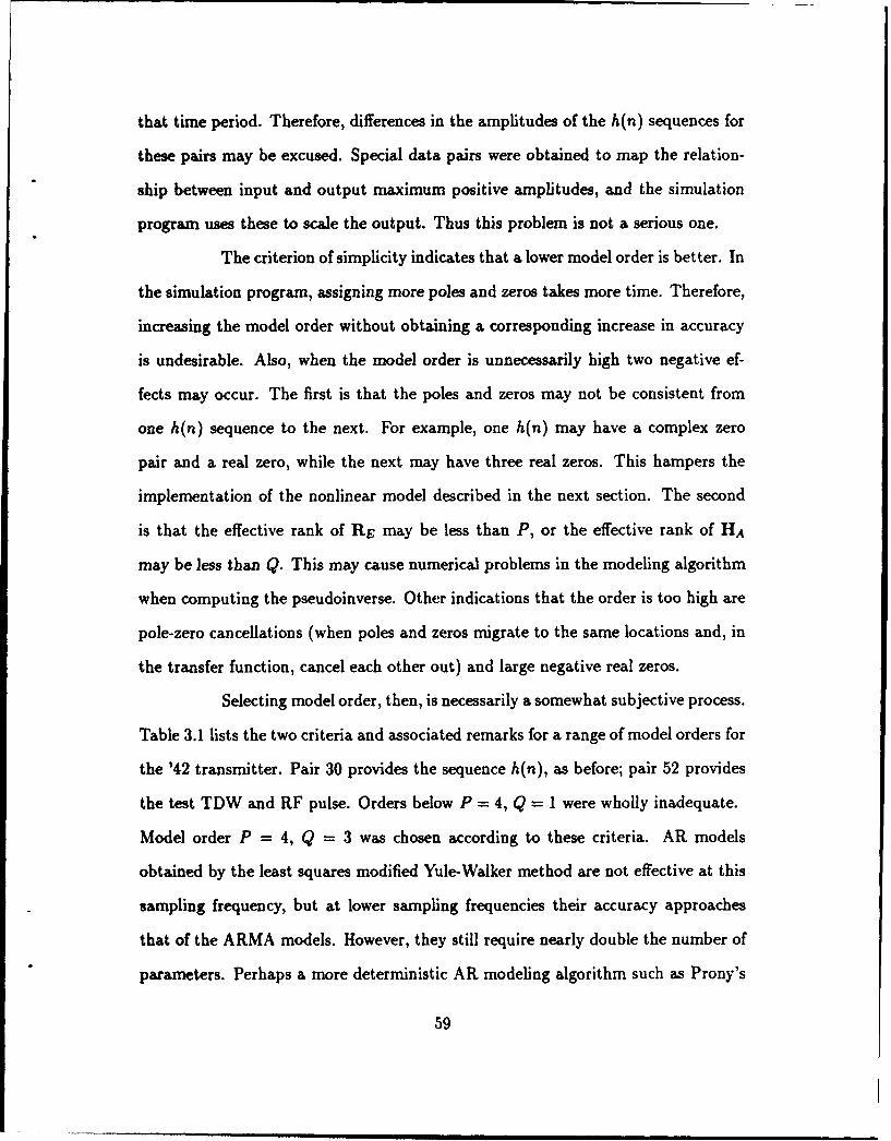
that time period. Therefore, differences in the amplitudes of the h(n) sequences for

these pairs may be excused. Special data pairs were obtained to map the relation-

ship between input and output maximum positive amplitudes, and the simulation

program uses these to scale the output. Thus this problem is not a serious one.

The criterion of simplicity indicates that a lower model order is better. In

the simulation program, assigning more poles and zeros takes more time. Therefore,

increasing the model order without obtaining a corresponding increase in accuracy

is undesirable. Also, when the model order is unnecessarily high two negative ef-

fects may occur. The first is that the poles and zeros may not be consistent from

one h(n) sequence to the next. For example, one h(n) may have a complex zero

pair and a real zero, while the next may have three real zeros. This hampers the

implementation of the nonlinear model described in the next section. The second

is that the effective rank of RE may be less than P, or the effective rank of HA

may be less than Q. This may cause numerical problems in the modeling algorithm

when computing the pseudoinverse. Other indications that the order is too high are

pole-zero cancellations (when poles and zeros migrate to the same locations and, in

the transfer function, cancel each other out) and large negative real zeros.

Selecting model order, then, is necessarily a somewhat subjective process.

Table 3.1 lists the two criteria and associated remarks for a range of model orders for

the '42 transmitter. Pair 30 provides the sequence h(n), as before; pair 52 provides

the test TDW and RF pulse. Orders below P = 4, Q = 1 were wholly inadequate.

Model order P = 4, Q = 3 was chosen according to these criteria. AR models

obtained by the least squares modified Yule-Walker method are not effective at this

sampling frequency, but at lower sampling frequencies their accuracy approaches

that of the ARMA models. However, they still require nearly double the number of

parameters. Perhaps a more deterministic AR modeling algorithm such as Prony's

59

TABLE 3.1: BASIS FOR SELECTING MODEL ORDER, AN/FPN-42TRANSMITTER

Measure 1 Measure 2P Q MSE NMSE Remarks

4 1 2.1069 x 10-4 1.2325 x 10-3

4 2 7.6821 x 10-5 1.2633 x 10-3

4 3 1.8948 x 10-5 9.0733 x 10- Best overall* *4 4 1.8314 x 10- 9.1274 x 10' 4th zero: at z -350 + j0

5 3 3.2620 x 10-5 8.8762 X 10-4

5 4 1.8585 x 10-5 8.9258 x 10-4

5 5 1.9309 x 10-5 7.4982 x 10-1 Mtx close to singular

6 3 5.5609 x 10-s 9.7328 x 10-4

6 4 1.8415 x 10-1 9.1727 x 10-4

6 5 4.6451 x 10-5 7.3653 x 10-4 Mtx close to singular6 6 1.1680 x 10-4 1.3550 x 10-3

10 0 2.9922 x 10-3 9.7445 x 10-2 AR models18 0 1.2797 x 10-3 4.5499 x 10-2

24 0 2.3607 x 10-3 7.3931 x 10-2

Method would produce better AR models [Ref. 15, pp. 88-89; Ref. 16, p. 550].

However, that is not the subject of this thesis. Completely deterministic ARMA

modeling (for example, using Prony's Method to find a and Shank's method to find

b) is not quite as effective here as the statistical/deterministic combination of the

least-squares modified Yule-Walker method and Shank's method.

60

E. NONLINEAR, TIME-VARYING MODEL OF THEAN/FPN-42 TRANSMITTER

1. Representing Nonlinearities by Moving Poles and Zeros

a. Changes in the Positions of Poles and Zeros Caused byChanges in TDW Shape

The transmitter's unit sample response changes slightly as the shape

of the TDW changes. The pole-zero models of these sequences are correspondingly

different also. The pole-zero scatter plot of five data sequence pairs in Fig. 3.7

illustrates this. All five were obtained within a period of three hours, avoiding time

variations in the transmitter. The length of time each TDW excited the transmitter

ranged from 5 jus to 80 jus, which provides a range of differently shaped TDWs.

The average MSE between h(n) and hAB(n) for these five pairs is 3.4641 x 10-6,

indicating an excellent match. This validates the assumption of LTI behavior at

operating points other than the typical one described previously.

b. Assigning Poles and Zeros by Parameter En

The apparent trajectories of the poles and zeros in Fig. 3.7 imply

that the transmitter may be simulated effectively by assigning the poles and zeros

of the model based on the shape of the TDW. In forming this catenated model a

reliable way is needed to relate the changes in TDW shape to the trajectories of

each pole and zero.

The energy of the normalized TDW (with the TDW's maximum

positive amplitude equal to one) can be used to assign poles and zeros according to

TDW shape. This energy, in units of watt-seconds, is defined as

E, = x(n)Tz(n)T (3.33){max [x(n)1}2R'

61

POLE/ZERO PLOT, PAIRS 22, 23, 12, 13, 141.5

...................... ....... ... ......... i........ ."...........

.... ... "... . . ....

• ... "",, - .. . .. ,.*.:. ,' ,

-0.5 ,. .. ,, .. : , ,, ..

tFigure 3.7: Pole-zero scatter plot for '42 with antenna simulator for fiveLTI models.

where sampling interval T is in seconds and load resistance R is normalized to

one. The choice of parameter E,, reflects an assumption that the most important

characteristic of the TDW shape is the length of time the TDW provides a significant

level of excitation to the transmitter. As observed before, transmitter behavior

changes significantly for TDWs that excite the transmitter longer than 100 jus, and

the transmitter no longer behaves linearly for TDWs that excite the transmitter

longer than 90 jus. It seems reasonable, then, to assume that the length of time

the TDW excites the transmitter is an important indication of transmitter behavior

also when this length is less than 90 pas. If the pole and zero locations are consistent

from one h(n) to another, if the poles and zeros form a fairly predictable trajectory

as they move with respect to E., and if the synthetic RF pulse y.(n) matches the

actual RF pulse l'(n), the approach using E,, may be considered valid.

62

Poles and zeros are assigned using E, as follows. First, the trajec-

tory of each pole and zero is assumed to be smooth and continuous, rather than a

series of discrete steps. The magnitude and phase of the kth root from each data

pair are plotted, so that there as many data points on the magnitude plot and the

phase plot of the kth root as the number of data pairs. A polynomial curve is fitted

to the points on both plots, and the process is repeated for each root.

A special MATLAB function MOD2 was written to fit these curves.

The user selects the order of the polynomial curve and may even add points at his

or her discretion to stabilize or bend the curve. The original points are denoted "o"

and any added points are denoted "*". When the user is satisfied with the curve, he

or she selects the minimum and maximum values of E,, and so defines the range over

which the curve is valid. The program stores these endpoints and the polynomial

values at the endpoints. These are used when assigning poles and zeros if E, falls

outside the endpoints. The coefficients ct, c- 1, -. , cl, co of the polynomial

ce(E.)" + ce. 1(E,- ) 1 - + ." + clE,, + co (3.34)

are stored as well. The curves fit by this program for the magnitude and phase of

the inner pole appear in Fig. 3.8. If the pole and zero locations in one h(n) sequence

are not consistent with those of other h(n) sequences, then that h(n) may create a

spike in one or more of the parameter curves. These outlier h(n) sequences may be

discarded to fit the curve more accurately.

When a TDW is presented to the MATLAB function XMTR, which

simulates the transmitter, the function first computes E" for the TDW. The func-

tion recalls in turn the stored coefficients of each polynomial, evaluates them at this

63

Magnitude of Selected Parameter

0.999colurnin 3

0.999

I 0.996 ......... ........

0.996°- . .........

0.998 i0 5 10 15 20 25 30 35 40 45

Energy of normalized input vector, watt-iec X 1e-6

(a)

Phase Vf Selected Parameter0.057

0.5 ... .. . . . ......... .... .. . ............... .....,......-....., ......celurro, 3

0.0517 .....- . .. ........... .........: ............. .........

0to.057 - - . ..... ..............- .................. i.......... ....Ii

0.057.

0 5 t0 15 20 25 30 35 40 45

Energy of normalized input vector, watt-tec X I -6

(b)

Figure 3.8: Fitted curves for inner pole pair, '42 with antenna simulator(5 pairs). (a) Magnitude, and (b) phase.

64

E., and combines these magnitudes and phases into poles and zeros. Vectors a and

b are then formed from these roots. Next, a unit sample and Eq. (3.2) produce

hAB(n), which is then convolved with z(n) to yield y.(n). Finally, the amplitude

of y°(n) is scaled appropriately, according to the input/output energy relationship

from special data pairs obtained for this purpose.

c. Performance of the Catenated Model

The catenated model, as implemented in the function XMTR, was

tested using the five data pairs described previously. As an example, the normalized

actual and synthetic RF pulses y(n) and y.(n) for pair 14 appears in Fig. 3.9. The

sequences are normalized because of the overall transmitter gain difference discussed

previously. The match is an excellent one; the plots of the other four pairs of y(n)

and y,(n) show about the same level of performance. The NMSE values between

y(n) and y.(n) for all five pairs appear in Table 3.2. As a basis for comparison,

the same tests are performed using the linear model of pair 30 developed earlier

in this chapter instead of the catenated nonlinear model. Table 3.2 also includes

these results. The simulation error of the nonlinear model is about an order of

magnitude smaller in these tests than the simulation error of a simple linear model,

for an average reduction of 93.4 percent. For data pair 14 the performance of both

models is about the same. These results validate this method of representing the

transmitter's nonlinearities &: demonstrate that the model accurately reflects the

transmitter's behavior over a wide range of operating points. This extra degree of

accuracy could make the difference between developing an algorithm that works on

the nonlinear transmitter and VXlbus control system and developing an algorithm

that does not. Next, the time variations of the transmitter are added to this model.

65

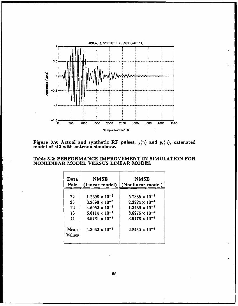
ACTUAL & SYNTHETIC PULSES (PAIR 14)

0.! t ............ ...... " ......... .. ............... " ............... ................ "" ................

-0.5 . .. ............... ... . ......... •. . ...... ...................... ........... ...........

................. . ...... : ... :................ ................. ................................... ........ 2..........:................ .................

0 500 1000 1500 2000 2500 3000 3500 4000 4500

Sample Number, N

Figure 3.9: Actual and synthetic RF pulses, y(n) and y,(n), catenatedmodel of '42 with antenna simulator.

Table 3.2: PERFORMANCE IMPROVEMENT IN SIMULATION FORNONLINEAR MODEL VERSUS LINEAR MODEL

Data NMSE NMSEPair (Linear model) (Nonlinear model)

22 1.2698 x 10-2 5.7835 x 10-4

23 3.2698 x 10-3 2.3224 x 10-4

12 4.6052 x 10-i 1.3439 x 10-4

13 5.6114 x 10-4 8.6276 x 10-514 3.9731 x 10-4 3.9176 x 10-4

Mean 4.3062 x 10-3 2.8460 x 10-4

Values

66

2. Representing Time Variations by Changing PolynomialCoefficient co

a. Changes in the Positions of Poles and Zeros Caused byTime Variations

Pole-zero models were produced for three data sequence pairs with

nearly identical TDWs, obtained over a period of nine months. Figure 3.10a shows

the first 1000 samples of the TDWs and Fig. 3.10b displays the pole-zero scatter

plot of the three pole-zero models. From Fig. 2.10b, it is apparent that time

variations in the transmitter's transfer function manifest themselves in the same way

as nonlinearities: by movements in the pole and zero locations of the IIR model.

These variations are about one-fourth the size of the variations due to changes in

TDW shape. From what is known about the transmitter's time variations, the

poles and zeros can be expected to drift slowly over hours, days and weeks. When

a different transmitter is switched on line, the pulse shape controller sees a step

change in pole-zero locations.

b. Moving Poles and Zeros Using Coefficient co

Changing coefficient co slightly in each polynomial as a function of

time t (every t1 iterations) is an effective way to model slow time variations in the

transmitter. As a result, each polynomial curve drifts up and down independently

of the others with respect to time t. This causes the poles and zeros to drift also

with respect to t. Introducing a larger random change in the co of each polynomial

implements a transmitter switch; the curves, and the poles and zeros, jump to a new

location. The size of the change to co is different for each curve, characteristically

small for the poles and larger for the zeros. Initially the maximum allowable change

of cD can be set to approximately one fourth the difference between the maximum

and minimum values of the polynomial curve in the valid range of E,,.

67

TOWS FOR PAIRS 5 (7/91), 8 (1/91), & 14 (2/92)

1 .32

0. .~ ...-. - - . .. ..... ..

0-0.51

1.5

-105 .

020 ..00 .0 . 0 1000.20

(a)

Figure ~ ~ ~ ~ OL/ZR 3LOT: (a)R Thre 8,~ 14o ar btie vra9-o eidfor ~ 1 '42. wihatnasmltr n b oezr cte lt

16

c. Simulating Slow Drifts Using an AR2 Random Process

The following AR2 random process driven by white noise produces

slow drifts generally in the range (-1, 1):

d(t) - 2(0.996)d(t - 1) + (0.996) 2d(t - 2) = w(t). (3.35)

Here d(t) is the output and w(t) is a white noise input with variance ',.25 x 10-1.

The system's double pole at 0.996 filters the noise and produces the slow drifts. The

exact value of these parameters were chosen by trial and error. An example output

d(t) over 1000 iterations appears in Fig. 3.11. Chapter V contains details on how

parameter drift is implemented in the simu! --tion program.

SLOW ORi7T d(t)0.8 ' - T rr T . . ..

. . ................. ... . . .. ............. .............. ... ......

0.24 ....... ... -.... . ...... ........ ........ .... -. ............. ... .. ... ... .......... ................ i...............

0.2 . ... ............. ; . . .... . .-.............. ................. ; ..............

-0.2

-0.4 10 100 200 300 400 500 600 700 8oo 900 1000

Iterotions, t

Figure 3.11: Slow drift produced by AR2 process.

3. The Combined Nonlinear, Time Varying Model

The catenated model from Subsection E. 1. and the time variations

described in E. 2. combine to form an accurate nonlinear, time-varying model of

69

the '42 transmitter. Only one more modification is necessary: the inclusion of all

the data pairs available. Figure 3.12 shows the magnitude and phase of the inner

pole (positive phase) using nineteen data pairs for the '42 transmitter. Appendix C

contains a complete set of these curves. As mentioned before, on occasion the user

may elect to remove one or more outliers; therefore all the points in the five-point

curves of Fig. 3.8 may not necessarily appear in these final curves.

From these curves, new maximum values of co may be determined sim-

ply by estimating a standard deviation of the data points by eye from the curve.

Granted, some of the deviation may be from nonlinearities as well as time vari-

ations. !U, however, the curve is allowed to drift to cover most of the points (it

will drift approximately one standard deviation from its normal position), the com-

bined model effectively duplicates nearly all the behavior observed in the data, both

nonlinearities and time variations.

The combined model thus meets the need for which it was designed: it

simulates all the observed nonlinear and time-varying behaviors of the transmitter

during the convergence of a pulse-shape control algorithm. As the control algorithm

changes the TDW shape, the model's transfer function changes also, just as the real

transmitter's transfer function does. This dynamic feature is essential for testing

control algorithms. One of its disadvantages, however, is that the simulation errors

of the combined model are now higher than those of the linear model. Tested with

all nineteen data pairs, the linear model's average NMSE is 2.8531 x 10- while

the combined model's average NMSE (without drift) is 1.0943 x 10-2, 284 percent

higher. Visually, however, y(n) and y,(n) for the combined model still match well.

Therefore, the value of the dynamic feature of the combined model outweighs the

disadvantage of the increased simulation error, and the combined model may still

be used with reasonable confidence despite this increased error.

70

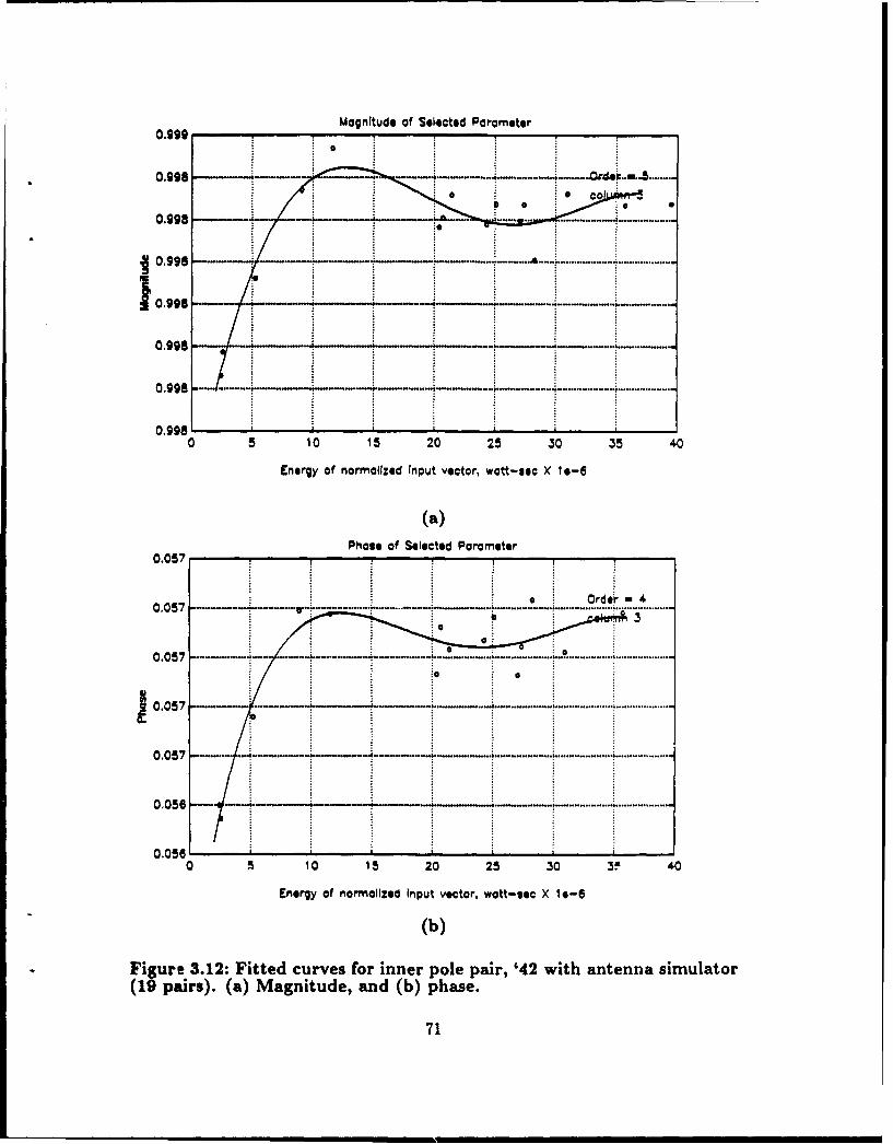
Magnitude of Selected Parameter

0.999 - ..-..

0.998 ..-. ........ .. .......

10.998

0,9918 _j ... & -........ ......................

0.998 6

0 5 10 15 20 25 30 35 40

Energy of norrmalized Input vector, wott-see X 1 e-6

(a)Phase of Selected Pararmeter

0.057 !'

* e Order 40.057 - - ---*-* * .----------------. .............

3

0.057.....................

0 .056 JLL

0 5 10 15 20 25 30 3F 40

Energy of normalized Input vector, watt-sec X le-6

(b)

Figure 3.12: Fitted curves for inner pole pair, '42 with antenna simulator(19 pairs). (a) Magnitude, and (b) phase.

71

Amplitude (V) E

Figure 3.13: Second AR coefficient a2 as a function of t and E,.

Finally, the combined model can be related to the linear difference equa-

tion with non-constant coefficients in Eq. 3.6. The simulation program stores only

the roots of a(t, E.) and b(t, E.), not the coefficients themselves. However, these

coefficients may easily be computed. For example, Fig. 3.13 shows a2(t, E") for

0 < t < 20 hours, and 2 x 10- _< E, < 40 x 10-6 watt-seconds.

4. Adding the Dummy Load to the Combined Model

Figures 3.14a and 3.14b show a data sequence pair for the '42 trans-

mitter connected to the resistive dummy load instead of the antenna simulator.

Figures 3.14c and 3.14d present sequences h(n) and hAB(n) and the pole-zero plot

corresponding to hAB(n) for model order P = 2, Q = 1. The time-domain match is

72

TOW: DUMMJY LOAD (PAJR 50)0.6•

-. 1

-0.4 -

-0. .. ..- ' '---"--- - --- * .. ..........-......

-0.4

0 500 1000 1500 2000 2500 3000 3500 4000 4500

Sample number, n

(a)

RI PULSE: DUMMY L0AO (PA)R 50)10 '

--- ---------____ -_ .- .........- .-. ....... ..... ..............S| I ,,....... I. . .I.

¶0

0 500 1000 1500 2000 2500 3000 3500 4000 4500

Sample number, n

(b)

Figure 3.14: '42 input and output, dummy load, pair 50. (a) TDW and(b) RF pulse.

73

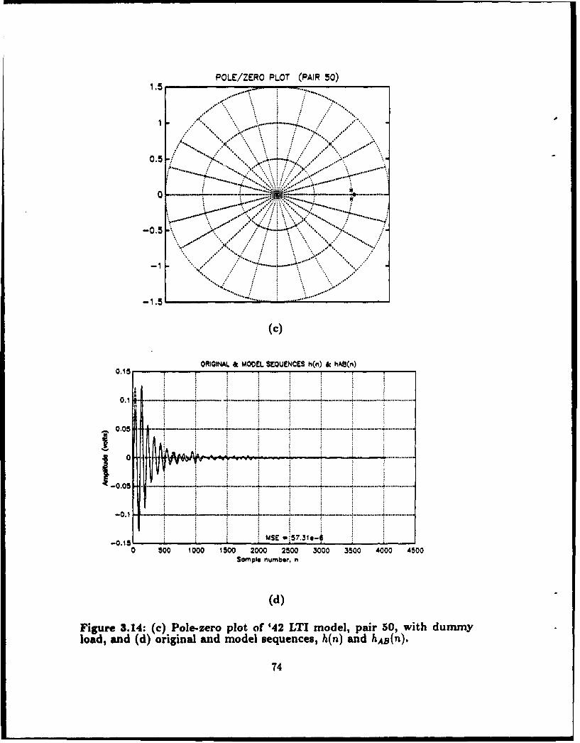
POLE/ZERO PLOT (PAIR 50)1.5 ........

%440.5/

, . . . ..-......... ".. . ...........0. 1, * .-.------- . . . .

0.5. ..... . ...o ...... ..".... . ..... ...... . ........

" " ROM -4 'v 0%64-: ..... .........

-0•.. 5 . ...... .. .... ..... ......4. .... . ... . .... ....... . . . .

-1 *~'**" E -;:57319-

S...!tra !!:.....

(d)

.C,..fG,...f.P.,Av.....v;..4..

I/ "../S" mple nu b ,, .". ...

Figure 3.14: (c) Pole-zero plot of '42 LTI model, pair 50, with dummyload, and (d) original and model sequences, h(n) and hAo(n).

T4

not quite as good as with the antenna simulator sequences because a lower model

order was chosen for the dummy load. Slightly higher model orders yield a modest

decrease in MSE but the locations of the poles and zeros are no longer consistent

and are thus unusable in the catenated model. As a result, order P = 2, Q = 1 is

used and is considered adequate. Appendix C also includes curves for these dummy

load poles and zeros.

F. NONLINEAR, TIME-VARYING MODEL OF THEAN/FPN-44A TRANSMITTER

The same procedure produced a combined model for the AN/FPN-44A trans-

mitter, with order P = 6, Q = 5. A linear model of typical pair 71 has the following

a and b:1.0000

-5.9652 0.050014.8348 0.010

a= -19.6972 b- 0.1019 (3.36)14.7246 -0.0514

-5.8759 0.01040.9779

The poles and zeros are

[ 0.9947e86 '8-59 Zeros = 1.0009e•°0 '10 3 1poles = .9986e':10- 5'9 zrs= 1.0025e'± 0.04 3 I.(3.37)

0.9956ej•' 45 19 1.0255ej J

All the data vectors for the '44A were obtained on the same day, so typical time

variations of this transmitter model were inferred. The combined model was tested

with fifteen data pairs against the linear model from pair 71, as before. The linear

model's average NMSE is 1.3059 x 10-2, and the combined model's average NMSE

is 5.0988 x 10-3. The catenated model thus reduces NMSE by 61.0 percent.

Figures 3.15-3.17 are the plots for the '44A modeling process. Appendix C

contains the pole-zero curves for the '44A.

75

POWER SPECTRUM 0 TOW (PAIR 71), "A XMTR180i

SNR: G04. dB

160

I120100-,

60 '

0 500 1000 1500 2000 2500

Sample number, k

(a)

POWER SPECTRUM OF RF PULSE (PAIR 71), "A XMTR200

SNR: 09.1 d1

180 . ....... . . . .;,

Sleo16! 0 -:•------ - - ...... ... ............... ° ....... ........ . ............

100

800 Soo !020 1500 2000 2500

Sample number, k

(b)

Figure 3.15: Power spectrum of '44A with antenna simulator, pair 71.(a) TDW and (b) RF pulse.

76

* CLOSEUP: POWER SPECTRUM OF TOW & RF (PAIR 7 1), "SA XMTR

ISO

IS

25 30 35 40 4 0 55 60

Sample number, k

Figure 3.15c: Closeup of power spectrum, 144A, pair 71i.

77

POLE/ZERO PLOT (PAIR 71)1.5........ .........

0.5

-0..

1.5 ..... . ....

(a)

ORIGINAL. & MODEL SEQUENCES h(¶) & hAS(m)0.04 1f'!

0.02 . ... ...... .. ...........

-0.01 .-*.....*-....4..-..-..-.-. .. . .............. .....................

-0.04 .............

-0.05MSE -:10.27o S0 500 1000 1500 2000 2500 .3000 3500 4000 4500

Sample numnber. m

(b)

Figure 3.18: (a) Pole-zero plot of '44A LTI model, pair 71, with antennasimulator, and (b) original and model sequences, h(n) and hAB(n).

78

TOW: DUMMY LOAD (PAIR 85)0.4 y- - - - - - -

0.3

0.2.- •' ' .... ............

0.1. . . . . . . . .

ow I1 el r, W ...............

-0.2 . ... ... _ _....... ..... .... . .........................

-0.30 500 1000 1500 2000 2500 3000 3500 4000 4500

Sample number, n

(a)

RF PULSE: DUMMY LOAO (PAIR 85)

0 ...............

0 500 1000 1500 2000 2500 3000 3500 4000 4500

Sample number, n

(b)

Figure 3.17: '44A input and output, dummy load, pair 85. (a) TDW and(b) RF pulse.

79

POLE/ZERO PLOT (PAIR 85)

,I ',, -.... " .. ,

0.5

-0.5- . . ."

(C)

ORIGINAL. A MODEL SEQUENCES h(m) & hAS(n)0.06 8%y~

0.0 . ... ....... - .. . .

0.04 ............ ..... . .. . -..

0.02 ........ 4........"" ,

v, "v . , / v V ...............

•-0-02 ........- / - ,. .,., . ......

-0.04~ ~ ~ ....... ..... ..... ..... ....... ..............

......... ...... .............. ...........

-00.MSE -7.222.6 50

Satmpe viumrn, n

(d)

Figure 3.17: (c) Pole-zero plot of '44A LTI model, pair 85, with dummyload, and (d) original and model sequences h(n) and hAS(n).

80

IV. THE STEEPEST DESCENT ALGORITHM

A. INTRODUCTION

This chapter presents an algorithm that generates and controls the Loran-C

pulse shape automatically. First, the Loran-C control problem is described. Second,

the algorithm is derived and its advantages and limitations are discussed. Finally,

the algorithm is successfully tested with the combined '42 and '44A transmitter

models from Chapter III.

B. PULSE SHAPE CONTROL IN LORAN-C

The VXIbus pulse shape control system (See Fig. 2.10) uses a batch pro-

cessing approach to monitor and control the Loran-C pulse shape. The oscilloscope

captures and stores in memory an entire RF pulse, or possibly an entire GRI or

even a PCI. A resident computer program reduces the waveform(s) to parametric

form, compares these parameters to the parameters from an ideal pulse, and pro-

duces a new TDW in parametric form. In the final step, the program expands these

TDW parameters into a digital data vector, which the AFG then converts into an

analog TDW. This operation constitutes one iteration of the Loran-C pulse shape

controller. The controller shapes the pulse by changing the TDW parameters to

minimize the error in the RF pulse parameters.

The simplest form of the controller uses a parametric form consisting of 16

TDW half-cycle peak amplitudes

xP = [xp(1), x,(2),..--, xrp(16)]' (4.1)

and 16 RF pulse half-cycle peak amplitudes:

y, = [y,(l),y,(2),- • • , ,(l6)]'. (4.2)

81

These are tracked in successive control iterations; Fig. 4.1 illustrates this for xp(3)

and yp(3). The half-cycle peak amplitudes of the ideal pulse of Eq. (2.1) are

Yop = [yop(1), yop( 2 ),. • - ,yop(1 6 )]', (4.3)

with output error vector

e. = y,- yop = [e,(1),e,(2),...,ev(16)1'. (4.4)

Thus the Loran-C pulse shape control problem is formulated as a 16-dimensional

regulator problem where yp, is maintained as close as possible to yop [Ref. 22].

C. THE STEEPEST DESCENT ALGORITHM

1. Derivation

A linear controller feedback which uses the method of steepest descent ef-

fectively shapes the Loran-C pulse by minimizing the quadratic error eTWe., where

W is a weighting matrix. In the steepest descent method, also used in adaptive fil-

tering, the error gradient is used to find the bottom of an error performance surface

[Ref. 19, p. 1971. The controller presented here is appropriately called the steep-

est descent algorithm in this thesis. This control algorithm, developed by Peterson

and successfully implemented in a hardware simulation by Steinvorth, is derived as

follows [Ref. 20, 21].

The transmitter is modeled as a linear system

Aoxp = yp, (4.5)

where A0 is the matrix of impulse response samples (peak amplitude samples are

used in this thesis):

h(o) 0 0 ... 0

Ao [Ph(l) hp(O) 0 ... 0 (4.6)

hp(16) hp(15) hp(14) hp(O)

82

Amplitude (V)

A n, x pl(3) • i

t

(a)

Amplitude MV)

A ny p(3) •-"I

t

(b)

Figure 4.1: Loran-C pulse shape control strategy. (a) Input and (b) out-put.

83

Let x% be the vector of optimum TDW half-cycle peak amplitudes. Multiplying the

true (but unknown) system matrix Ao and optimum TDW half-cycle peak vector

xop yields the ideal pulse peaks:

Aoxop - yop. (4.7)

Let

e, = xP - xoc (4.8)

be the vector of errors in the TDW half-cycle peak amplitudes. Beginning with A,

the best estimate of Ao, the first vector of TDW half-cycle peak amplitudes is

xpLl= A+yop. (4.9)

Vector Axp updates xp at each iteration t in the direction of steepest descent on the

quadratic error surface defined by erWey:

Ax P=-LV [eTWe.], (4.10)

where p is a small constant greater than zero and Vejxfi] is the vector of partial

derivatives of scalar K with respect to the elements of e,.

Equation (4.10) may be expanded to the form

Axp = -! Ves[feAo WAoex]. (4.11)

20

Diagonal matrix W weights the elements of e. and e,. W = I weights all the errors

equally, while a W whose diagonal elements decrease in size from upper left to lower

right implements a tighter tolerance in the first part of the pulse. Equation (4.11)

then becomes

Ax -= -pAoWAoex, (4.12)

then

x= -pAWe.. (4.13)

84

Matrix A, which is known, is substituted for unknown AD, resulting in the steepest

descent algorithm

Iax, = --pATWe, . (4.14)

For negatively phase coded pulses the "- sign is removed. Finally, if [ATWAo]-1

is positive definite and

2

P largest eigenvalue of [ATWAol' (4.15)

the system is stable.

2. Advantages and Limitations

The algorithm of Eq. (4.14) has two main advantages and two pri-

mary limitations. The algorithm's advantages are its effectiveness and its simplicity.

As the next section shows, the algorithm works well for the data available. Also,

the simple parametric form allows the algorithm to be implemented with only two

(16 x 16) matrix multiplications per iteration (with 768 real multiplications and 512

real additions). The algorithm's limitations are its assumption of an overall linear

controller system and its inability to control zero-crossing times. By using small

values of p and a standard 16-half-cycle TDW, the controller keeps the transmit-

ter confined to an approximately linear region. If the controller is also "tuned" by

updating A from time to time to compensate for time variations, the first limita-

tion is not a serious one. The second limitation simply requires the zero-crossing

times to be adjusted as they have always been: by keeping the transmitters well-

maintained and well-tuned to 100 kHz. This limitation imposes no extra burden on

Loran-C operation or maintenance, so likewise it is not a serious one. Admittedly,

having an algorithm that adjusts zero-crossing times automatically would be quite

advantageous, but this capability is not absolutely necessary in order to implement

automatic pulse shaping successfully.

85

D. CONTROLLING PULSE SHAPE IN THE COMBINEDMODEL USING THE STEEPEST DESCENT ALGO-RITHM

The steepest descent algorithm effectively generates and controls the Loran-C

pulse peak amplitudes in the combined models of both the '42 and the '44A. The

zero-crossing tolerances were met for the '42 but not the '44A.

Figures 4.2a through 4.2d illustrate the performance of the steepest descent

algorithm with the '42 combined model without time variations. Figure 4.2a shows

the smooth convergence of the mean squared error e~ey for the first 100 iterations,

and Fig. 4.2b presents the convergence of three measures of Loran-C error for the

same 100 iterations. These are the half-cycle peak amplitudes (ensemble tolerance)

and the half-cycle peak amplitudes (individual tolerance) for half-cycles 1-8 and

for half-cycles 9-13. The temporary rise in mean squared error from iteration 10

through 18 in Fig. 4.2a is a result of linearly controlling a nonlinear system. Figures

4.2c and 4.2d show the first 800 samples of the ideal and synthetic RF pulses after

100 iterations. All half-cycle peak amplitudes of the initial TDW (at iteration t = 1)

were set to 0.4 volts. In these plots, normalized p

largest eigenvalue of [ATWAI (4.16)

2

is set to 0.7. Next, beginning with iteration 101 and ending with iteration 200,

time variations are introduced at each iteration. This approximates a 25-hour pe-

riod. These figures demonstrate the algorithm's ability to compensate for slow time

variations in the transmitter's transfer function.

Figures 4.4 and 4.5 illustrate similar success with the '44A except that zero-

crossing times are not within tolerance. Half-cycle peak amplitudes 15 and 16 of

the fin.al TDW are larger, to fill out the end of the controlled part of the pulse, but

86

101 Convergence of Output MSE

1 0 -f :~... ~..........1

............

100 ¶ 0 3 0 5 0 7 0 9 0

... . .........

.0- . ....

10 O 10 ..0. .0 40.. ..0 .0.0.8.90 10

. ... .. ... ..... ...r.t..o......

(b).....

Figure~~~~~~~~~ ~.. 4.2 Tetngseeet.ecet....t.wih'4.ndaten..aConvergence~~~~ of mensqae error.. ......ad.().onerenc.o.tre

mesrso Cora rgn-ce eror.min roMxers15 a rs911087

Final Transmitter Drive Waveform (tdw)

AN/FPN-42 10 M~ Anifnna00 Itorations Drift. 101/1

0.4 ------------ .1 * - .. . ....... .......

-0.4

0 100 200 300 400 500 600 700 8500 900

Sample number, n

(c)

30Ideal &Synthetic ftF Outputs (beginning at 1st half cycle)AN/FPN-42 . 10 kI4j Amtinno

100 itorations Drift. 101/1

-20............

In tolOiancsW I-JL

0 10 200 300 400 ;00 600 700 800 900

Sample number, n

(d)

Figure 4.2: Testing steepest descent algorithm with '42 and antenna. (c)Final TDW and (d) ideal and synthetic RF pulses.

88

Convergence of Output MSE

10-24

MKZ .. .I A t rý....... ........ ........io .S 00.. 8 .0.. : .. .... ..................................

. ........ ..... ..............

10-31 j~.. i

100 110 120 130 140 150 160 170 180 190 200

Iterations, t

(b)

'42. (a) Cnverence of mnebean-squaredx error 1- Mand (rrs Conergncof three. mesue of.. Loa- error.... .........

89......

x10-3 Orift Parometers (including possible step ¢hongee)3

---- ----------------- ------ - i

2 ' -- -----" "--.--- "- " :--'- --- .........-.. ". .............. .. . ........... -- ............. ---- .......-- '-'-"-- - ......

0--~~~~ ~~ 1 . . .- ... . . .- : . .." .. ......... P ............ ..... ......... ...............

.. ....... .... ......................-2 ..-h • _ .•_ • . .. _ ........ ...... : .... .........

-3---

- 4.-.....4 . 4 ..... .*, ....

-5 ---- ----- ------ -' "' ----

100 110 120 130 140 150 160 170 180 190 200

Iteration, t

Figure 4.3c: Testing steepest descent algorithm with time-varying model,'42, drift parameters (co coefficients).

this has an unintended effect with the '44A combined model. This is because the

tail drive decays exponentially starting from the amplitude of half-cycle 16. With

such a large 16th half-cycle, the tail of the TDW contains almost as much energy as

half-cycles 1-14. If actually implemented, half-cycles 15 and 16 could be attenuated

to compensate for this problem. Also, the phase difference in Fig. 4.4d reflects

the change in transmitter delays that may be produced by time variations in the

transmitter's transfer function. As stated before, emission delays are not addressed

in this simulation.

These figures show that the steepest descent algorithm effectively shapes the

Loran-C pulse. However, these tests of the algorithm are unrealistic because com-

plicating factors such as noise, quantization error and power supply droop are not

included. Also, only one pulse of the PCI has been controlled. In the next chapter,

90

the combined models of Chapter III and the steepest descent algorithm are incorpo-

rated into a comprehensive simulation program which does provide a realistic test.

Experimental results from the simulation program are also included.

i~~~~o ~~Convergence of Output USE........e ........

........................ .... . ...... . ......................

....... ....................................

. -. --- - --. ---- ....................4.... . . 4........................... ...........

10 .. .~~..... .................................. .... I... . . . . ........... ...... ... ....... ..........1 . . ....!.......... .......... ...........

. . ...l..... ....... ........... !..............S.............................? ............. . ....... ................

. . . . . . . ...... .................. . . .........

.......- ................... -4.. .......................

. ~ 4 ......... . . . . . . . .

.~no ...... ..01 1 .. ft . 10... 1 . ........ ........ ..........i...............................

----0 -10 ..0 30 ... 0. . 0 60.... 70 .0 90 100.................. ............

10-31

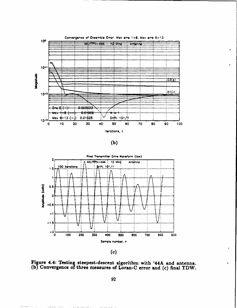
Convergence of Ensemble Error. Max errs 1 -a, Max erms 9-13

...............---.. i.- -. -- .................

.......... .......................................... 10 20....... 30...0...0.....70..80..0..100...r...... .t........... .................

( b ). ...................

.. .................-.5 . / ....... .................

1 -2 -0

-- -------..1..................... ....

........... ;J L ..................0.... .0 200. ..00.400..00..00...00..0....0

Sa pl n--m----r- n.................

.(e) .... ........ ............... ur 4.4 Tesin steet-ecn a.. gorithm wit ........ an antenna...............................

Convegenc of three. measures............. of.Lor...C.error.and .(c).final.TDW92 ..............................

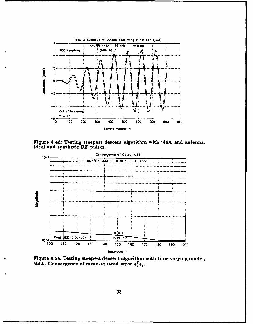
Ideal &Synthetic RIF Outputs (Ibeqirnl~im at 13t half Cycle)AN/PPN-44A 10 MNj Antinna

100 iterations Drift: ¶0/1

1~ 3

Out of talerancoE

0 100 200 300 400 500 600 700 800 900

Sample number, n

Figure 4.4d: Testing steepest descent algorithm with '44A and antenna.Ideal and synthetic RF pulses.

10-2 Convergence of Output MSE

..................... ...... . . ............. .............

. .. ......... .......... ..........

...... .a ... ............. .... .................. ...........

. . . . . . . . . .-------. -.----. . . ...............

100 110 120 130 140 150 160 170 1S0 190 200

iterations, t

* Figure 4.5a: Testing steepest descent algorithm with time-varying model,'44A. Convergence of mean-squared error e~'e~.

93

Convergence of Ensemble Error, Max err 1-8, Max errs 9-1310-' .........

S.. ...• .... ... 6. .........." ....... . 6 ................. ............ "" . . ........ . ................ "............ ............ ........-- .. . . .. .. . ... i . . . ...... .. .... .... .......................... ................. I................ .

iu I uuma I i I - i

10-2 r

• .• •- .. .................... .. .............................

S.... . . .. & • .. f • . .. • -.-..-- .-.-... ... , ............. .. .............. ............... .

S....... ... ....... ... .. . ... ..... : ..... . .. :.- .... .. .................... ... ................ i................171). • -0 s ... . .4 .... . ..... ......... .............. ........ ................. ;.................

Max 1:. -s ) 0.011736 W ýw IMax• 9ý1 O-'j4 D-'i: o1o/1 1 ,:,

100 110 120 130 140 150 160 170 180 190 200

Iterations, t

(b)

x10" Orift Parameters (including possible step changes)10

j ui ~iiiii:uizz :z iiS. .. . . • . -- _.. _ __ _ _................

46: : •, ,.. -. • . . ....... • ............ .•.............. ............. .

"2 ........ ---- - .......I

-2'

100 ¶10 120 130 140 180 ¶60 I "0 180 190 200

Iterations. t

Figure 4.5: Testing steepest descent algorithm with time-varying model,'44A. (b) Convergence of three measures of Loran-C error and (c) driftparameters (co coefficients).

94

V. SIMULATION PROGRAM AND RESULTS

A. INTRODUCTION

In this chapter the models of Chapter III and the control algorithm of Chap-

ter IV are incorporated into a comprehensive MATLAB computer program which

simulates the pulse-shaping control process on the AN/FPN-42 and AN/FPN-44A

transmitters. Also, key results obtained from this simulation program are featured.

B. THE SIMULATION PROGRAM

1. Structure

The diagram in Fig. 5.1 shows the basic structure of the simulation

program. In brief, the user selects the options for the simulation run, including

which pulses of the PCI he or she wishes to control. For each of the selected

pulses, the program completes a specified number of control iterations. A control

iteration consists of obtaining the RF pulse, determining the error in the RF pulse

parameters, and producing a new TDW. After the iterations are finished, a pulse

analysis is performed and the program moves to the next selected pulse. This

program simulates controlling the shorter rate of a dual-rated station, and from

time to time the rate is blanked. When this occurs, the controller skips an entire

control iteration and does not increment the loop counter. Thus the blanking process

is simulated but is invisible to the pulse shape controller.

2. Explanation of Features Appearing on Main Menu

a. Main Menu

The user controls the simulation program through a main menu,

which appears in Fig. 5.2. Using this menu, the user ,)nfigures the transmitter and

95

SInltialze

USer selectsOpon

ScomSeleted

Analyze pulses

done?

Figure 5.1: Basic structure, simulation program.

96

LORAN-C TUBE TRANSMITTER SIMU1LATION

(c) Dean C. Bruckner & Murali Tummala, 1992

1. Transmitter: AN/FPN-42 2. Xmtr load: Dummy Load3. Sampling freq: 10.00 MHz 4. Local ECD: 0.00 us5. Resolution: 8 bits 6. Imbalance: 0.007. W. Noise pct: 0.39 8. Reset Xmtr9. Pulses to control: 1 1

10. Pulses to analyze: E 1 111. Number of iterations: 100 (1st pulse), 20 (following pulses)12. Xmtr parameter drift occurs every 0 iterations with norm mag. 113. Xmtr switch occurs every 0 iterations (1st pulse only, when drift on)14. Display method: plot15. Control algorithm: Steepest Descent16. Display/change current algorithm parameters17. Access keyboard 18. Exit

Enter number(s) to change parameters or <Enter> to begin:

(e.g., 1 or [1 7 8]) ====>

Figure 5.2: Main menu, simulation program.

control algorithm and selects the desired display, analysis and recording options. In

this section each menu item is briefly explained.

b. Transmitter Selection

The user may select either the AN/FPN-42 or the AN/FPN-44A

transmitter. The program loads the polynomial coefficients for the selected trm.ns-

mitter, which have been stored in a single matrix with one polynomial in each row,

as in Fig. 5.3. The polynomial coefficients of the kth root appear in adjacent rows -

the first for magnitude and the second for phase. The program reinitializes variables

governing the transmitter's operation and resets the drive waveforms and control

algorithm.

97

c. Transmitter Load

The simulation program operates with either the antenna or the

dummy load. The polynomial curves for the dummy load are in the lower partition

of the matrix in Fig. 5.3. The program implements a load switch by resetting a row

pointer for this matrix to select either the upper or lower partition. In its default

mode, the program uses the dummy load to produce a near-optimum TDW for the

antenna. The program switches to the antenna when the output errors fall below a

threshold. This minimizes the time the pulse is out of tolerance when transmitting

on the antenna. The "ideal" dummy load RF pulse used in this process was obtained

by allowing the algorithm to converge on the antenna, switching to the dummy load

and recording the output of this TDW. After switching to the antenna, usually the

RF pulse is in tolerance within an iteration or two. Here the antenna and antenna

simulator are used interchangeably.

Row

Magnitude ct ct-1 C1- 2 ... co

Phase 4f 4 -1 4-2 ... CO Antenna(root k)

Dummy

Load

Figure 5.3: Polynomial coefficient matrix.

d. Sampling Frequency

This program runs at four data sampling frequencies: 10 MHz, 5

MHz, 2.5 MHz, and 1.25 MHz, as discussed in Chapter III, Subsection D.1. The

best error convergence is at!. =10 MHz, but the program runs the fastest and

requires the least storage at f1 = 1.25 MHz. The algorithm resets the transmitter

and control algorithm when a new sampling frequency is selected.

98

e. Local ECD

The program controls the local (transmitted) ECD of the RF pulse

by generating a new ideal Loran pulse with the desired ECD from Eq. (2.1) and

using the new pulse in the control algorithm. Currently in the Coast Guard, ECD is

controlled by inserting a phase shift called the Early Timing Adjust (ETA) into the

TDW. This program bypasses the ETA altogether and successfully controls ECD

to within 0.44,us in the range -2.5jis <7r < 2.51us by changing the ideal waveform.

The LOIS program, used in the daily Loran-C system sample, is used to measure

ECD by hand.

f. Amplitude Resolution and System Noise

The simulation program incorporates the noise model shown in Fig.

5.4. The noise present in the actual data pairs may be duplicated in simulation by se-

lecting eight-bit quantization and adding white noise to the synthetic TDW and

Sq .'bit XMTR Sq - bitquantizer quantizer [

white ] ,whitenoise Sq .'bit noise

(var. 1) quanfizer (var. 2)1

Record MDW

Controller

Ideal RF Record RF

Figure 5.4: Transmitter system noise model.99

TABLE 5.1: AVERAGE SNR OF MEASURED DATA PAIRS(ANTENNA)

SNR (dB)Transmitter TDW I RF Pulse

AN/FPN-42 56.4 62.0

AN/FPN-44A 56.1 66.6

RF pulse until the SNRs of both match the average SNRs of the actual data (as

defined in Chapter III, Subsection B.2.b.). These average SNRs are listed in Table

5.1.

Because the relative amplitudes of the '42 and '44A waveforms are

different, the standard deviation of the white noise is expressed as a percentage

of the maximum positive amplitude of the waveform. The SNRs in Table 5.1 are

achieved in simulation using the settings in Table 5.2.

The user specifies the number of bits and the noise percentage of

the RF pulse in menu items five and seven, respectively; the program then sets the

TDW noise percentage automatically by multiplying the RF pulse noise percentage

by 2.7 for the '42 and 1.8 for the '44A. Other quantization settings available are

Sq = 12 bits, Sq = 16 bits and S. = oo (maximum resolution, to machine precision).

These represent a best-case scenario, because all the quantization levels are used.

In the real system, some of the levels at the top and bottom are not usually used to

avoid saturation, reducing the effective bit resolution. The capability to reproduce

the observed noise level in the transmitter system is extremely important as it allows

the simulation to be a realistic one. Results of different quantization settings are

presented in Section C of this chapter.

100

TABLE 5.2: PROGRAM SETTINGS WHICH REPRODUCE SNR OFMEASURED DATA

Std. Dev. of White NoiseNumber of (% of peak amplitude)

Transmitter bits, Sq TDW RF Pulse

AN/FPN-42 8 1.05 0.39

AN/FPN-44A 8 0.97 0.54

g. Transmitter Imbalance

As described in Subsection C.l.e. of Chapter II, an imbalance be-

tween the two vacuum-tube amplifier banks in a transmitter reduces the amplitude

of the negatively phase coded pulses. The program simulates this imbalance by

reducing the amplitudes of these RF pulses by a percentage defined by the user

in this menu item. The program automatically compensates for this imbalance by

increasing the TDW amplitude by an appropriate amount. As with ETA, the phase

code balance adjustment in the PGEN is bypassed entirely.

h. Reset Transmitter

When the program completes controlling and analyzing all the se-

lected pulses in a PCI, the main menu appears again and the user has the option to

continue where the program left off. The reset feature allows the user to start the

control process from the beginning again without exiting the program. When the

user selects this item, the program resets the drive waveforms, the control algorithm

and the random transmitter drift settings (if drift is enabled), but it leaves intact

the other control and analysis settings in the main menu.

101

i. Pulses to Control

The program can control any or all of the pulses in a PCI, as speci-

fied by the user. The TDWs for all selected pulses of the PCI are stored in successive

columns of matrix D., which represents a data output buffer to the AFG. The con-

trol approach is sequential, beginning with the first selected pulse. The program

"drives" the transmitter model by presenting the TDW in column one of D, as an

input argument to the function XMTR. The resulting RF pulse is in turn presented

as an input argument to the control algorithm, which produces the new TDW. This

TDW, which is the best estimate of the optimal TDW for each pulse, is loaded into

all the columns of D, and proper phase-coding is applied. The amplitude of each

TDW may also be scaled up exponentially to compensate for power supply droop as

explained later in this section. When the specified number of control iterations are

completed, the final RF pulse is stored in column one of matrix RI and the program

moves to the next selected pulse. As the program controls the pth pulse, columns p

and following of D, are updated every iteration, but columns one through p - 1 are

not. When the entire process is completed, matrix D, contains the best estimates

of the optimal TDWs for all selected pulses, and R, contains the selected output

RF pulses. In the VXIbus system, the output data buffer can easily be dumped to

the AFG. With an MPT to set the proper time of emission, the desired TDW would

be sent to the transmitter.

j. Pulses to Analyze

When the program finishes controlling an RF pulse, it performs an

analysis of that pulse and the control process that produced it. The program's

default setting is to analyze every selected pulse, but the user may suppress any

or all of these analyses. The program then prints the results to a screen and to

an ASCII text file, as in Fig. 5.5. Next, the program plots the Loran-C errors and

102

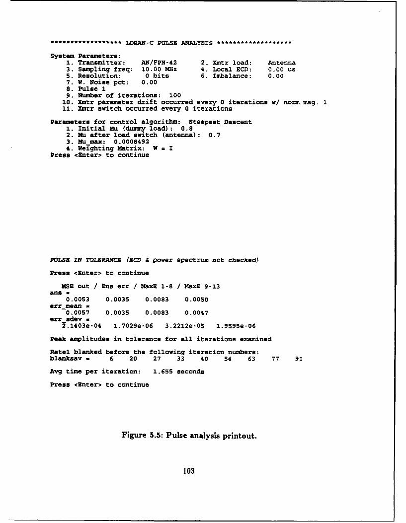
****************** LORAN-C PULSE ANALYSIS *

System Parameters:1. Transmitter: AN/FPN-42 2. Xmtr load: Antenna3. Sampling freq: 10.00 MHz 4. Local ECD: 0.00 us5. Resolution: 0 bits 6. Imbalance: 0.007. W. Noise pct: 0.008. Pulse 19. Number of iterations: 100

10. Xmtr parameter drift occurred every 0 iterations w/ norm mag. 111. Xmtr switch occurred every 0 iterations

Parameters for control algorithm: Steepest Descent1. Initial Mu (dumuy load): 0.82. Mu after load switch (antenna): 0.73. Mu max: 0.00084924. Weilghting Matrix: W = I

Press <Enter> to continue

PULSE IN TOLERANCE (ECD & power spectrum not checked)

Press <Enter> to continue

MSE out / Ens err / MaxE 1-8 / MaxE 9-13ans -

0.0053 0.0035 0.0083 0.0050err-mean =

0.0057 0.0035 0.0083 0.0047err sdev a

2.1403e-04 1.7029e-06 3.2212e-05 1.9595e-06

Peak amplitudes in tolerance for all iterations examined

Ratel blanked before the following iteration numbers:blanksav = 6 20 27 33 40 54 63 77 91

Avg time per iteration: 1.655 seconds

Press <Enter> to continue

Figure 5.5: Pulse analysis printout.

103

Normalized pulse peak valuesaverage, last iter, ideal, diff (1-3), diff (2-3)

ans =

0.0074 0.0074 0.0157 -0.0083 -0.0083-0A0793 -0.0793 -0.0833 0.0041 0.00410.1915 0.1915 0.1901 0.0013 0.0014

-0.3180 -0.3181 -0.3158 -0.0022 -0.00230.4470 0.4471 0.4454 0.0016 0.0017

-0.5711 -0.5712 -0.5696 -0.0015 -0.00160.6828 0.6828 0.6813 0.0014 0.0015

-0.7782 -0.7781 -0.7771 -0.0010 -0.00100.8584 0.8584 0.8556 0.0028 0.0028

-0.9211 -0.9214 -0.9164 -0.0047 -0.00500.9625 0.9631 0.9598 0.0027 0.0033

-0.9856 -0.9861 -0.9872 0.0015 0.00111.0000 1.0000 1.0000 0 0

-1.0067 -1.0064 -1.0001 -0.0066 -0.00630.9965 0.9965 0.9892 0.0073 0.0073

-0.9668 -0.9675 -0.9692 0.0024 0.0017

SNR (tdw) = 83.93 dBSNR (rf) = 108.3 dB

Figure 5.5 (continued): Pulse analysis printout.

output mean squared error, the final TDW and RF pulse, the rest times and esti-

mated power supply voltage (explained later in this section), and the drift parame-

ters. These plots are also recorded in META file format.

k. Number of Iterations

Here the user selects the number of control iterations for the first

selected pulse and for all following pulses. The default setting for the first selected

pulse is 100, which is usually sufficient time for the algorithm to converge. Because

the TDWs of the following pulses are also replaced every iteration during the con-

vergence of the first selected pulse, the pulses are in tolerance or nearly in tolerance

104

at their first control iteration. Bringing these errors into convergence thus requires

fewer iterations and so the default setting is twenty iterations.

1. Transmitter Drift

In this item, the user sets both the time scale and the magnitude

of the transmitter parameter drift described in Chapter III, Subsections E.2. and

E.3. Setting td = 300 and the normalized magnitude equal to one reasonably ap-

proximates the time variations in an actual transmitter. Reducing the value of td or

increasing the normalized drift magnitude artificially increases these time variations,

which is useful in testing and analysis.

m. Transmitter Switch

By introducing a random step change into the co parameters shown

in Fig. 5.3, a switch to a different transmitter may be simulated. The program

performs transmitter switches at a regular interval, as often as the user desires. In

this way, the algorithm may be tested with an infinite number of different '42 and

'44A transmitter models as no two random settings of the co parameters are exactly

alike. When the number of iterations per transmitter switch is set to zero, however,

the identical transmitter model is produced every time. To obtain a random setting

and to disable time variations, the user sets the number of iterations per transmitter

switch to the number of control iterations (menu item 11) plus one. The load remains

the same during a transmitter switch. The performance of the control algorithm

following transmitter switches appears in Section C of this chapter.

n. Display Method

To monitor the errors as the algorithm converges, the user may

select the text line option of Fig. 5.6a or the plot option of Fig. 5.6b. Or, the

105

Iter # / 3SE out / Ens err / MaxE 1-8 / MaxE 9-13taP w

1.0000 0.4163 0.0219 0.0356 0.0230Iter # / cSE out / Ens err / MaxE 1-8 / MaxE 9-13

taP =2.0000 0.4163 0.0219 0.0356 0.0230Iter # / MSE out / Ens err / MaxE 1-8 / MaxE 9-13

tMP =3.0000 0.3029 0.0268 0.0428 0.0160Iter # / 1SE out / Ens err / MaxE 1-8 / MaxE 9-13

tMP =4.0000 0.2578 0.0266 0.0434 0.0128

(a)

Convergence of Ensemble E"or, Max errs 1-B. Mox errs 9-13

" .- . .... R .... .............................. ..... .......... .. ........... . ..........................S. . ............. ................ .................. ... ......... .... .

.............. - ----------- -- ----- : ................ .. ... ... . .. . . ......

10-2 01 (r)

... .... ...... . ... ............. . ............... .................... ....... . ................10- .. .... ............

.4...- . .................. ...... ................

S...... • . . . ..• . . •.-... .. ..... _ ...... ...... ......... ................. :............. .... ... .............. •... ......

- ------- --- - .............. ... . .......... .............. ...............10 -3 .........o.. ,.. =o ••........

0 1 0 20 30 4.0 50 60 70 80 90 1 00

Iterotions$, t

(b)

Figure 5.6: Options for displaying error convergence. (a) Text line, andplot.

106

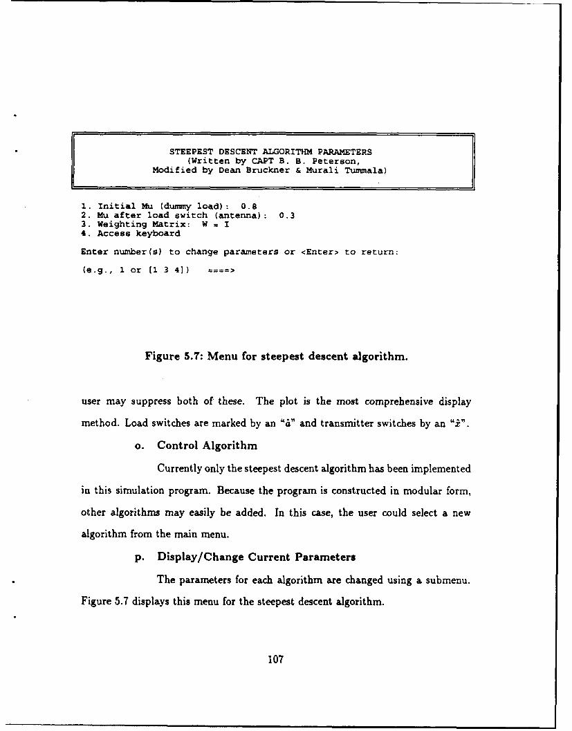
STEEPEST DESCENT ALGORITHM PARAMETERS(Written by CAPT B. B. Peterson,

Modified by Dean Bruckner & Murali Tummala)

1. Initial Mu (dummy load): 0.82. Mu after load switch (antenna): 0.33. Weighting Matrix: W = I4. Access keyboard

Enter number(s) to change parameters or <Enter> to return:

(e.g., 1 or [1 3 4]) ===>

Figure 5.7: Menu for steepest descent algorithm.

user may suppress both of these. The plot is the most comprehensive display

method. Load switches are marked by an "a" and transmitter switches by an ".

o. Control Algorithm

Currently only the steepest descent algorithm has been implemented

in this simulation program. Because the program is constructed in modular form,

other algorithms may easily be added. In this case, the user could select a new

algorithm from the main menu.

p. Display/Change Current Parameters

The parameters for each algorithm are changed using a submenu.

Figure 5.7 displays this menu for the steepest descent algorithm.

107

q. Access Keyboard

In this option, the user accesses the MATLAB command line. Here

he or she may examine or change parameters not accessible at the menus.

3. Explanation of Features Not Appearing in the Main Menu

a. Simulating Power Supply Droop

The problem of power supply droop has a negative effect on a closed

loop Loran-C control system, as described in Subsection B.2.d. of Chapter II. The

amplitude of each successive pulse in a GRI is reduced by a small amount, because

the power supply of the transmitter does not fully recover within the 1000 ps pulse-

to-pulse interval. This program models the power supply voltage Vp. as a charging

exponential with four parameters:

* The normalized power supply voltage just prior to the last pulse (vt, in the

range (0,1),

e The decrease in power supply voltage due to transmitting the last pulse (Avi),

e The time the power supply has rested since the last pulse (t"), and

e The time constant of the charging exponential (,r,).

These are shown graphically in Fig. 5.8. It was first assumed that the transfer

function of the transmitter changed measurably with decreases in the power supply

voltage; however, an analysis of an entire GRI revealed no predictable changes in

pole and zero locations. Therefore, the effect of droop is modeled solely as a decrease

in RF pulse amplitude.

The quantity vp, is estimated before obtaining each RF pulse. In

the function XMTR, the RF pulse is multiplied directly by the vp, estimated for

that pulse. This simulates the decrease in amplitude due to droop. Quantities Arv

108

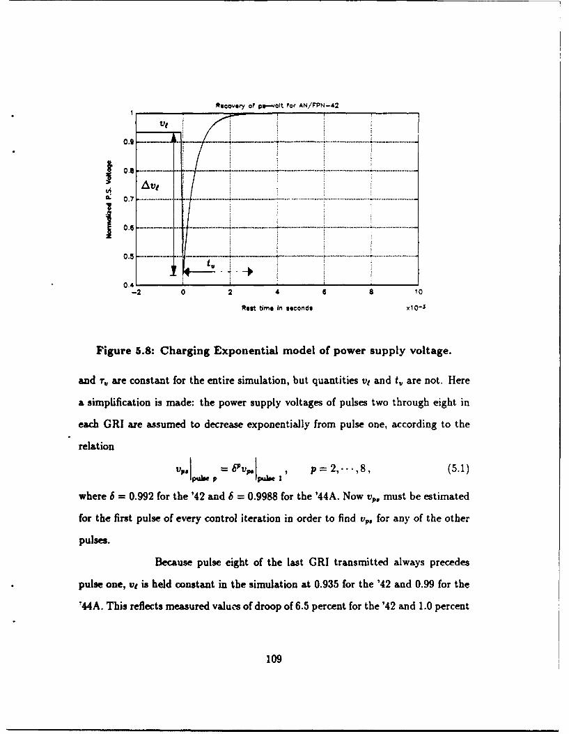
Recovery of p9-volt for AN/FPN-42

0.2 ..... ....... -.-- '• • • .... .* ..........

Ave

.... ........ ... . .............. ... ......................... , ...... ................. •.......................... .........................O~0.70.6...o ......... ...... ... ...... .... ........................ .... ..................................

0.5 ..... .. .... 4 - - ... ......... ............. ...........

0.4

-2 0 2 4 6 8 10

Rest time In seconds xl 0-3

Figure 5.8: Charging Exponential model of power supply voltage.

and r,, are constant for the entire simulation, but quantities v, and t,, are not. Here

a simplification is made: the power supply voltages of pulses two through eight in

each GRI are assumed to decrease exponentially from pulse one, according to the

relation

v, I, = PVP-P I p= 2,...,', (5.1)

where 6 = 0.992 for the '42 and 6 = 0.9988 for the '44A. Now vp. must be estimated

for the first pulse of every control iteration in order to find Vp. for any of the other

pulses.

Because pulse eight of the last GRI transmitted always precedes

pulse one, vj is held constant in the simulation at 0.935 for the '42 and 0.99 for the

'44A. This reflects measured valucs of droop of 6.5 percent for the '42 and 1.0 percent

109

for the '44A. Realistic values of variable t. for each control iteration, however, are

found only by simulating dual-rated operation.

b. Simulating Dual-Rated Operation

As explained in Chapter II, Subsection B.4., a dual-rated station

transmits GRIs for two adjacent chains, and the two GRIs are not synchronized

to each other. When the blanking intervals enclosing the GRIs overlap, one of the

rates is blanked. When the blanking intervals are very close to each other but do

not overlap, however, the droop of the power supply is accentuated. In this case,

the transmitter transmits eight pulses spaced 1000 lss apart followed by a rest as

short as 1900 ps, which is then followed by eight more pulses spaced at 1000 us.

The interval between the two GRIs is the quantity t,.

A problem arises when the VXIbus control system happens to sam-

ple a pulse in this second GRI. The peak amplitude of the sampled pulse from this

GRI will be noticeably smaller than the average peak amplitude of that pulse from

other GRIs. This introduces a transient disturbance into the control algorithm. The

purpose of including dual-rate operation in this simulation is to study the response

of the control algorithm to these transient effects.

The MATLAB function REST was written to produce a vector of

consecutive rest times t,, in seconds, prior to the GRIs of the shorter rate in a

dual-rated station. For two secondary rates 99,400 ps and 59,900 ps, 200 samples

of this vector are plotted in Fig. 5.9. From this figure, the periodic nature of this

function is clear. In this program the pulse shape controller captures a pulse from

a GRI every four seconds; with 66 GRIs in a four-second period, realistic values of

t,, for pulse one in each GC1 are thus obtained by taking every 66th sample from

the vector of rest times. Another vector of the same length bt, indicates the samples

110

CONSECUTIVE REST TIMES

0.07

0.06

0.05

I0.040.03-

0.02

0.01

0 20 40 60 60 100 120 140 160 180 200

Group Repetition Intervols

Figure 5.9: Vector of consecutive rest times, 200 samples.

for which the shorter rate was blanked; if the controller encounters one of these, it

records the blanked iteration (see Fig. 5.5) and skips that GRI altogether.

Vector t, is 503 samples long; when the end of the vector is reached

the counter wraps around to the beginning again. Because 503 is a prime number,

all of the samples in the vector should eventually be used if the simulation continues

long enough. Figures 5.10a and 5.10b show the error convergence plots for a '42

simulation run of 100 samples. The controller switches from the dummy load to

the antenna at iteration 24. Figures 5.10c and 5.10d show the estimated values

of t, and vp. for each iteration. The increase in error is clearly visible between

iterations 29-32. Fortunately, the algorithm is able to compensate and these errors

are transient.

111

Convergence of Ensemble Error, Max arms 1-8, Max errs 9-13

..... ........... ..... 4. . ............... *... * .......... ........

...... £.(- .. J . ..7......i........

M---x- ---8 ..-) .7 ....... ...................

................................... ........ ....... .............

................................

Final trrasE 035 r 0

0 10 20 30 40 50 60 7 0 9 0

Iterations, t

(a)

(b)~Cnerec thre measure ofLraSrrr

100 .112

Recovery Times for first pulse in GR1, rotelI0.06

rate 1 140.0599;: rot*2-0.099* ato-id-SS iPulseI

0.0! - . ... u.

0.04

0.01'

01Min rust-0OOO2127 s _____

0 10 20 30 40 50 60 70 80 90 100

Iterations, t

(c)Estimated Power Supply Voltage (normnaliZed)

..9..- -- -....... '.... .. .........

I 0.996 - .............................

0.994 .......

Min p v-0-9980.992

0 10 20 30 4.0 50 60 70 80 90 100

Iterations, t

(d)

Figure 5.10: Effect of transient disturbances, continued. (c) Rest timesand (d) estimated power supply voltage.

113

c. Exponential Scaling of TDW Amplitudes

In order to speed the convergence of pulses two through eight of the

GRI, the program anticipates the droop of the transmitter. It boosts the ampli-

tude of each successive TDW slightly when storing the TDWs in buffer matrix D,

according to the relation

(TDW)j, =P(DW)1 , p = 2,..., 8, (5.2)

where / = 1.02 for the '42 and O = 1.0015 for the '44A. These values are not exactly

the inverses of the 6 values given earlier; no specific a priori knowledge of droop was

assumed, and these values were obtained experimentally. This feature does in fact

speed convergence; in most cases, pulses two through eight converge within two to

three iterations.

C. RESULTS

1. Realistic Simulation of the AN/FPN-42

In a realistic simulation of the '42 with 600 control iterations, the steepest

descent algorithr shaped the Loran pulse effectively but maintained the pulse peaks

in tolerance for only 78.3 percent of the control iterations in a test interval beginning

at interation 101 and ending at iteration 600. The zero-crossings and ECD of the

final RF pulse were in tolerance, however. The system noise drove the pulse peaks

out of tolerance repeatedly. These out of tolerance cases would not necessarily

require blink, but they are undesirable. Whether or not this would be acceptable

in actual Loran operation is a policy matter for the Coast Guard to decide. In

any case, these fluctuations are an indication that the steepest descent algorithm is

sensitive to noise and that it is not as robust as perhaps it should be. Figures 5.11 a

through 5.llg are the plots for the first 100 iterations of this run; Fig. 5.11h is the

printout for the test interval.

114

100 Convergence of Output USE

P .. .. ...7 ....10-...............

.........

..na .4S .1 ......... */ ............0.. 10 20 30 ..0 50....... 60 70 80 ...... 90.... 100..

I .- ~ ..--. 4........

4 -..............-. .

~ ~ ...........-....

A I . . . .: r........ .....

.. Eat-..... . on~~a ....... M fl.k ....................... .... ...f -.......

Max~~- -~- -----: -~3 -- -- -------- -

Fin3 al -14SE 0.02117 Drift: 0/1 i bits=8

0 10 20 30 40 s0 s0 70 80 90 100

Iterations, t

(b)

(b) 1 threnmas rgnes of Lornsml error. a rs18 a rs 1

115.....

Mum.5 0. ~Fina Transmitter Drive Waveform (tdw)0.6 ~ &0. AN/FPN-42 10 MHj Ant nna Pulse' I

100 it~irations Drift: 0/ 1

-0.2

taumO noise-0.397. bits-S

0 100 200 300 400 500 600 700 800 900

Sample number, n

(c)Ideal & Synthietic RF Pulses (begirinirig at lst half cycle)

30Muii0i.i & o.3 AN/FjPN-42 10 MH! Antenna Pulse I

100 itqrations Drift: 0 1

20 ...- . .... ....... .. ...... . .................

1 0 ..... /.... .. .... .. .... .. ..... ........

W - I tou-0 Inoise-10.39% bits-S300 100 200 300 400 500 600 700 800 900

Sample number, n

(d)

Figure 5.11: Realistic simulation results, '42. (c) Final TDW and (d)ideal and final synthetic RF pulses.

116

Recovery Times for first pulse in GRI, rate 10.06

rat* 1 IP0.0599:.ý rot*2inQ.0994 soiSSPulse

0.05 . . ...

I 0.03 -- --

0.02--.. ..

Min re two 002627 sod0

0 10 20 30 40 50 60 70 80 90 100

Iterations, t

(e)Estirmated Power Suooly Voltoge (normolized)

..99 .. ........... ..... -...... ................ ... . . .... ............................

0.999 ................................. .......

o .99a -.. .1 .- . .*... . ..............

0 in.998.9t

0.9970 10 20 30 40 50 60 70 80 90 100

Iterations, t

Mf

Fiqure 5.11: Realistic simulation results, '42. (e) Rest times and (f)estimated power supply voltages.

117

Drift Parameters (including possible step changes)0.06

0.02 - - • - . . . . . . . . . -. . ........ ........ .i.............. .................

-0.04 . ..... ... ...............-, * - •.. . . ............................. .. "...............................,

-0.02

-0.04 .. .- -

0 10 20 30 40 50 60 70 80 so 100

Iterations, t

Figure 5.11g: Realistic simulation results, '42, drift parameters.

118

****************** LORAN-C PULSE ANALYSIS ****************

System Parameters:1. Transmitter: AN/FPN-42 2. Xmtr load: Antenna3. Sampling freq: 10.00 MHz 4. Local ECD: 0.00 us5. Resolution: 8 bits 6. Imbalance: 0.007. W. Noise pct: 0.398. Pulse 19. Number of iterations: 10010. Xmtr parameter drift occurred every 0 iterations w/ norm mag. 111. Xmtr switch occurred every 0 iterations

Parameters for control algorithm: Steepest Descent1. Initial Mu (dummy load): 0.82. Mu after load switch (antenna): 0.33. Mu max: 0.00084924. Weighting Matrix: W = I

Press <Enter> to continue

PULSE IN TOLERANCE (BCD & power spectrum not checked)

Press cEnter> to continue

MSE out / Ens err / MaxE 1-8 / MaxE 9-13ans a

0.0212 0.0047 0.0085 0.0133err-mean =

0.0249 0.0069 0.0113 0.0092err sdev a

Y.8736e-02 3.3487e-02 4.3991e-03 4.0186e-03

Peak amplitudes in tolerance for 83.6 % of iterations examined

Ratel blanked before the following iteration numbers:blanksav -

10 23 37 51 56 70 81 83 94

Avg time per iteration: 3.59 seconds

Press <Enter> to continue

Figure 5.11h: Realistic simulationresults,'42, pulse analysis printout.

119

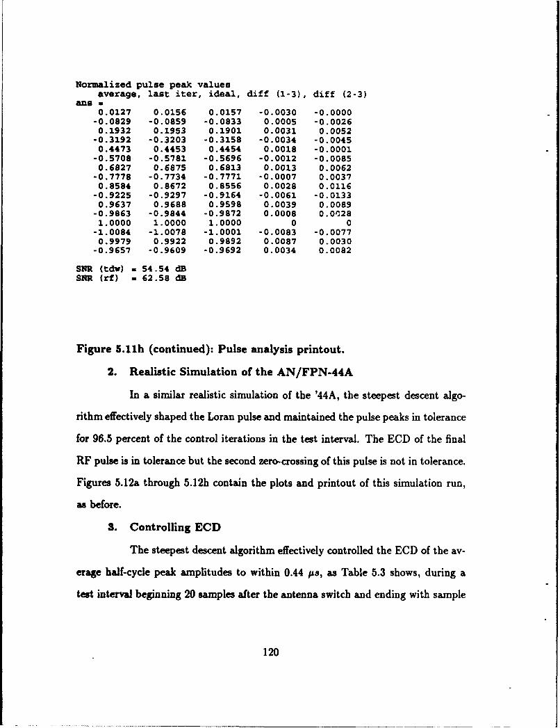
Normalized pulse peak valuesaverage, last iter, ideal, diff (1-3), diff (2-3)

ars a0.0127 0.0156 0.0157 -0.0030 -0.0000

-0.0829 -0.0859 -0.0833 0.0005 -0.00260.1932 0.1953 0.1901 0.0031 0.0052

-0.3192 -0.3203 -0.3158 -0.0034 -0.00450.4473 0.4453 0.4454 0.0018 -0.0001

-0.5708 -0.5781 -0.5696 -0.0012 -0.00850.6827 0.6875 0.6813 0.0013 0.0062

-0.7778 -0.7734 -0.7771 -0.0007 0.00370.8584 0.8672 0.8556 0.0028 0.0116

-0.9225 -0.9297 -0.9164 -0.0061 -0.01330.9637 0.9688 0.9598 0.0039 0.0089

-0.9863 -0.9844 -0.9872 0.0008 0.00281.0000 1.0000 1.0000 0 0

-1.0084 -1.0078 -1.0001 -0.0083 -0.00770.9979 0.9922 0.9892 0.0087 0.0030

-0.9657 -0.9609 -0.9692 0.0034 0.0082

SNR (tdw) = 54.54 dBSNR (rf) = 62.58 dB

Figure 5.11h (continued): Pulse analysis printout.

2. Realistic Simulation of the AN/FPN-44A

In a similar realistic simulation of the '44A, the steepest descent algo-

rithm effectively shaped the Loran pulse and maintained the pulse peaks in tolerance

for 96.5 percent of the control iterations in the test interval. The ECD of the final

RF pulse is in tolerance but the second zero-crossing of this pulse is not in tolerance.

Figures 5.12a through 5.12h contain the plots and printout of this simulation run,

as before.

3. Controlling ECD

The steepest descent algorithm effectively controlled the ECD of the av-

erage half-cycle peak amplitudes to within 0.44 ps, as Table 5.3 shows, during a

test interval beginning 20 samples after the antenna switch and ending with sample

120

Convergence of Output MSE

10 ~ . ..lfI ..... JpBfIa nluju.. n:..... .3,3:I~f3f

'10

.. J. ....

O0 10 20 .0 ..0....60..0..80 90 100

...... .. .... ...

P in ......-..........--..............

.................. ....... ..........GIQQ 4......-d .1,a. ... . ...........-

-Mow4-O-(--~ ~ du.4.........-... .o e 4 ..

Mox-2- 3 C-.n 0-0 3;! nrf 0/ bmitn0nmi m0 20 30... .0.060 70..90 .0

.traio s ...........HP -------..........

Figure~~~~~~~~~~~~ 5.2:Ralsicsmuato-rslt,----()-en-qarderoand ~=4 (b) the me.sres.f.Loan.eror

10-3 1 ...121

Final Transmitter Drive Wavefarvvi (tdw)

MuM0.4 & 0.3 A/FPýN-44A 10 MHz Anitenna PUlSQ 1

CA -.......... ,.. I ......

21taumO noise-0.54V% bits=S

0 100 200 300 400 500 600 700 800 900

Sample number, n

(C)Ideal & Synthe.tic RF Pulses (beginning at 1st half cycle)

MumO.6 & 0.3 AN/ PN-44Aj 10 MHz: Antinna Pulse:I100 itqroticne r? 0/1

4 ...............* ................

2-4 - - . .. ......

Sample number, n

(d)

Figre .12 Relisicsimulation results, '44A. (c) Final TDW and (d)ideal and final synthetic RE pulses.

122

Recovery rlime* for first pulse in GRI, rate 10.07 roe 1009; rt260p us

0.05

0.04 K0.03 -

0.02 . . .. .... *...... .

M~in ruestmo 00?427 sei01

0 10 20 30 40 50 60 70 80 go 100

Iterations, t

(e)Estimated Power SUPPly Voltage (nornmoliZed)

2 YiYPulse

lMim pjVM1_______010 10 20 30 40 50 60 70 80 go 100

Iterations, t

Mf

Fiqure 5.12: Realistic simulation results, '44A. (e) Rest times and (f)

estimated power supply voltages.

123

Drift Parameters (including possible step changes)0.06 ....

0.04 - - - - ,- -- ••".. . .. ;. ..... ". .. . • • • m . . .. .. ... . ...............

0.02 -

-0.02 --

-0.04 --

-0.06 , A.0 10 20 30 4.0 50 60 70 80 90 100

Iterations, t

Figure 5.12g: Realistic simulation results, '44A, drift parameters.

124

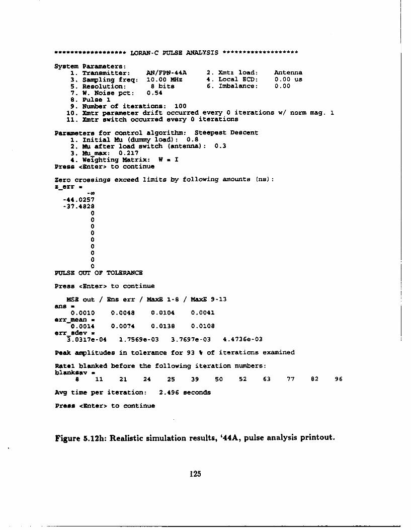
****************** LORAN-C PULSE ANALYSIS ****************

System Parameters:1. Transmitter: AN/FPN-44A 2. Xmtz load: Antenna3. Sampling freq: 10.00 MHz 4. Local ECD: 0.00 us5. Resolution: 8 bits 6. Imbalance: 0.007. W. Noise pct: 0.54S. Pulse 19. Number of iterations: 100

10. Xmtr parameter drift occurred every 0 iterations w/ norm mag.11. Xmtr switch occurred every 0 iterations

Parameters for control algorithm: Steepest Descent1. Initial Mu (dummy load): 0.82. Mu after load switch (antenna): 0.33. Mu max: 0.2174. Weighting Matrix: W = I

Press <Enter> to continue

Zero crossings exceed limits by following amounts (ns):z err

-44.0257-37.4828

000000000

PULSE OUT OF TOLERANCE

Press <Enter> to continue

14E out / Ens err / MaxE 1-8 / MaxE 9-13ans -

0.0010 0.0048 0.0104 0.0041err mean =

0.0014 0.0074 0.0138 0.0108err sdev -

3.0317e-04 1.7569e-03 3.7697e-03 4.4736e-03

Peak amplitudes in tolerance for 93 V of iterations examined

Ratel blanked before the following iteration numbers:blanksav =

8 11 21 24 25 39 50 52 63 77 82 96

Avg time per iteration: 2.496 seconds

Press CEnter> to continue

Figure 5.12h: Realistic simulation results, '44A, pulse analysis printout.

125

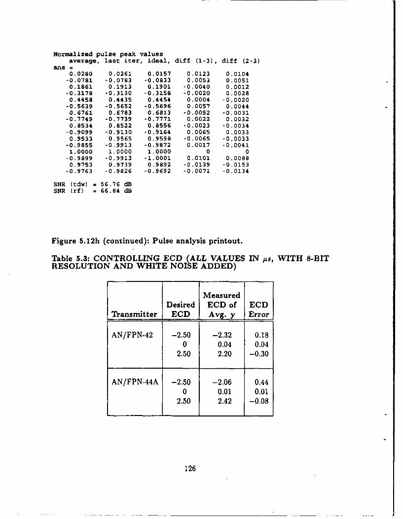
Normalized pulse peak valuesaverage, last iter, ideal, diff (1-3), diff (2-3)

ans =0.0280 0.0261 0.0157 0.0123 0.0104

-0.0781 -0A0783 -0.0833 0.0053 0.00510.1861 0.1913 0.1901 -0.0040 0.0012

-0.3178 -0.3130 -0.3158 -0.0020 0.00280.4458 0,4435 0.4454 0.0004 -0.0020

-0.5639 -0.5652 -0.5696 0.0057 0.00440.6761 0.6783 0.6813 -0.0052 -0.0031

-0.7749 -0.7739 -0.7771 0.0022 0.00320.8534 0.8522 0.8556 -0.0023 -0.0034

-0.9099 -0.9130 -0.9164 0.0065 0.00330.9533 0.9565 0.9598 -0.0065 -0.0033

-0.9855 -0.9913 -0.9872 0.0017 -0.00411.0000 1.0000 1.0000 0 0

-0.9899 -0.9913 -1.0001 0.0101 0.00880.9753 0.9739 0.9892 -0.0139 -0.0153

-0.9763 -0.9826 -0.9692 -0.0071 -0.0134

SNR (tdw) = 56.76 dBSNR (rf) = 66.84 dB

Figure 5.12h (continued): Pulse analysis printout.

Table 5.3: CONTROLLING ECD (ALL VALUES IN pa, WITH 8-BITRESOLUTION AND WHITE NOISE ADDED)

MeasuredDesired ECD of ECD

Transmitter ECD Avg. y Error

AN/FPN-42 -2.50 -2.32 0.180 0.04 0.04

2.50 2.20 -0.30

AN/FPN-44A -2.50 -2.06 0.44

0 0.01 0.012.50 2.42 -0.08

126

100. The realistic settings of Table 5.2 were used here also, with p,, = 0.7. ECD

values were measured by hand using the LOIS program, which accepts the first

eight half-cycle amplitudes as its sole input arguments. The error converged to

lower values for positive ECDs than for negative ECDs.

Because ECD was not computed for each iteration, the maximum ECD

error and the variance of the ECD errors are not available. Therefore, the precise

effects of noise and quantization error on ECD are not known.

4. Performance Improvement With Greater Bit Resolution

Table 5.4 presents the improved performance with the '42 that results

from adding more quantization levels to the Sq-bit quantizer in the noise model of

Fig. 5.4. A 600-iteration test was conducted as in Section B of this chapter, with

the same test interval (iterations 101-600). Bit resolutions Sq = 7 and Sq = 10

were set manually using the keyboard. Resulution Sq = 7 represents a worst case

for the VXIbus system, where the waveform's amplitude spans only half the vertical

oscilloscope scale and uses only 128 of 256 quantization levels available. Resolution

Sq = 8 represents the best case where all 256 levels are used. The actual performance

of the system should lie in between these two, closer to Sq = 8.

Three measures of the algorithm's performance were selected for this

comparison: the SNRs of both TDW and RF pulse, averaged over all iterations

in the test interval; the percentage of iterations in which the pulse peaks are in

tolerance; and the mean and standard deviation of the half-cycle amplitude error

(ensemble tolerance). The maximum allowable value for this third measure is 0.01.

The ensemble tolerance was chosen because it is usually exceeded first out of all of

the pulse peak amplitude tolerances. The variance of the white noise remains the

same, from Table 5.2.

127

Table 5.4: PERFORMANCE IMPROVEMENT WITH GREATER BITRESOLUTION ('42 TRANSMITTER, WITH WHITE NOISE ADDEDAND pn = 0.3)

% ofAverage Iter. Half-Cycle Peak

Bits SNR in Tol. Ens. ErrorSq TDW RF (peaks) Mean Std. Dev.

7 54.0 59.9 79.8 0.0085 0.0036

8 54.2 62.1 78.3 0.0077 0.0037

10 54.2 63.3 87.1 0.0065 0.0039

12 54.2 63.4 86.3 0.0065 0.0034

16 54.2 63.4 81.9 0.0070 0.0037

oo" 54.2 63.4 81.2 0.0071 0.0040

" To machine precision.

Although the accuracy of this simulation where Sq # 8 is not supported

by any data (to date, no oscilloscope for the VXIbus exists with more than eight

bits), Table 5.4 shows a marginal improvement in all measures with S -= 10, but

the performance worsened for higher values of Sq. This is because quantizing into

discrete levels removes completely the noise with amplitude less than one-half the

bin width. Additional filtering is thus appropriate for all values of Sq. Similar results

should be expected for the '44A.

5. Performance Improvement with Less Noise

Reducing the variance of the white noise allowed the steepest descent

algorithm to keep the pulse peaks in tolerance consistently with the '42, while still

using quantization with 8 bits. Using the same test procedure (used in Chapter IV

and in the first part of this chapter) reducing pt from 0.7 to 0.3 did reduce the

128

steady-state errors but did not increase the SNRs. The improved performance is

apparent in Table 5.5.

TABLE 5.5: PERFORMANCE IMPROVEMENT WITH LESS NOISE('42 TRANSMITTER, WITH 8-BIT RESOLUTION AND p=, 0.3)

RF Average % of Iter. Half-CycleNoise SNR in Tol. Peak Ens. Error(%) TDW RF (peaks) Mean Std. Dev.

0.39 54.1 62.1 78.3 0.0077 0.0037

0.25 57.9 64.7 92.5 0.0060 0.0024

0.20 59.8 65.7 95.2 0.0056 0.0020

0.15 62.1 66.7 98.3 0.0053 0.0014

0.10 65.3 67.9 100 0.0049 0.0009

To precision of machine

An acceptable solution may not necessarily require the pulse peaks to

meet the criteria in the signal specification for 100 percent of control iterations. The

rminimum acceptable performance level and the method of reducing system noise are

thus both subjects for further study. A similar performance improvement may be

expected with the '44A.

6. Behavior Following a Transmitter Switch

The steepest descent algorithm converges to the same degree as above

after switching to a different '42 transmitter of which it has no specific a priori

knowledge. In Fig. 5.13, iterations 1-75 show the error convergence for a trans-

mitter with realistic settings whose co coefficients have been randomly displaced

129

as discussed in Subsection D.2. of Chapter III. At iteration 76, the coefficients are

changed again, simulating a switch to a different transmitter. The algorithm's quick

response shows that it is versatile enough to use with transmitters at other Loran

stations in the Coast Guard. Similar performance was seen with the '44A. Again,

system noise prevents the error from converging any further.

7. Controlling the Entire PCI

The steepest descent algorithm also performed well in controlling an

entire PCI in a realistic simulation with a 3.0 percent transmitter imbalance intro-

duced as well. Here p,, = 0.7. The pulse-to-pulse ECD and amplitude tolerances

from Chapter II, Subsection B.2.e. were easily met. The shortcomings of the con-

trol algorithm in dealing with noise appear also in pulses two and following, but the

features of the program designed to control these pulses worked successfully. The

program controlled ECD without ETA, compensated for droop without a separate

droop correction circuit, and corrected phase code bounce without a separate phase

code balance adjustment.

130

Convergence of Ensemble Error, Max errs 1-8, Max errs 9-1310-1 1.-

~~~~~.. .. . H I"M - ' ' ...

• ,• ... . ...... ...... .....

.... ..[ '. ' r"i la ii 5 I . ... ... . . ...... . ... ..

I It I il V , ow pll I 1A f ^I ^ I r

..•,L•,• •._ o • __ •,• •.•-: •-: •..... •....=-• ......... .......

Max i-e C--): o0.01560 W . noiso0.s9IMax 9-13 0.01284 Drot: 151/1 bits-8:

0 20 40 60 80 o00 120 140 160

Iterations, t

Figure 5.13: Algorithm performance after transmitter switch at

iteration 76.

131

[THIS PAGE INTENTIONALLY LEFT BLANK]

132

VI. CONCLUSIONS

A. CONCLUSIONS

Modernizing the control systems for Loran-C vacuum-tube transmitters re-

quires a control algorithm to shape the Loran pulse automatically, and in this thesis

an algorithm was adapted for this purpose. In order to test the algorithm fully and

to provide a tool for future study, a detailed simulation program for two classes of

tube transmitters, the AN/FPN-42 and AN/FPN-44A, was developed. This pro-

gram incorporates discrete-time IIR models of each transmitter.

Based on an initial assumption of LTI behavior at a given operating point,

a linear difference equation with non-constant coefficients was chosen to represent

the dynamics of the transmitters. Frequency-domain deconvolution, in conjunction

with median smoothing, yielded an accurate estimate of the unit sample response

at each operating point. Next, the least squares modified Yule-Walker method and

Shank's method provided a non-minimum phase pole-zero model of each sequence.

These models were catenated to represent the transmitter's nonlinearities, and time

variations were added to form a combined model. The non-constant coefficients

of the difference equation were defined as functions of time and the energy of the

normalized TDW. The accuracy of this model was then demonstrated for both the

'42 and the '44A transmitters.

Next, a linear feedback controller which uses the method of steepest descent to

minimize the quadratic output error was derived, and its advantages and limitations

were discussed. The algorithm successfully shaped the pulse with both the '42 and

the '44A by bringing the pulse peaks into tolerance, although zero-crossing tolerances

were exceeded in some cases. Then, the models and the control algorithm were

133

incorporated into a simulation program. To this program were added the details of

the Loran transmitter system which affect pulse shape. Finally, the algorithm was

tested in a variety of transmitter system settings and behaviors. From these tests,

four main conclusions can be made.

First, based on all the data available, the MATLAB simulation program and

the nonlinear, time-varying models it contains accurately represent the behavior of

the '42 and '44A transmitter systems over the range of operating points used. The

assumption of LTI behavior at each operating point is a valid one, and the model

reproduces it faithfully. The de~ails of Loran operation added to the program make

the simulation a realistic one. Therefore the results obtained are directly applicable

to the VXIbus system.

Second, the steepest descent algorithm shapes the pulse effectively in realistic

simulations of both the '42 and '44A transmitters, with two significant shortcomings:

the zero-crossing tolerances are exceeded occasionally with the '42 an,' always with

the '44A, and the algorithm is sensitive to system noise. This noise drives the pulse

peaks out of tolerance frequently. Still, under these conditions, the algorithm kept

the ECD of pulse one in tolerance and quickly produced an entire PCI which met the

pulse group tolerances for amplitude and ECD, even when a transmitter imbalance

was added. Further, the algorithm reshaped the pulse effectively after transmitter

switches.

Neither of these two shortcomings necessarily disqualify the algorithm even

as presently implemented, for two reasons. The first reason is that the ability to

control zero-crossing times is not an absolute requirement for a pulse-shaping algo-

rithm. The second reason is that the acceptable level of error for the VXIbus control

strategy has not yet been defined. Of course, improvements in these two areas will

make the algorithm even more useful. With respect to reducing noise, if the SNRs

134

of the TDW and of the RF pulse can be improved by 10 dB and 5 dB, respectively

('42), the algorithm will keep the pulse peaks in tolerance continuously.

Third, power supply droop at dual-rated stations introduces only transient

errors into the algorithm's convergence. This causes the controller no significant

problem.

Fourth, a near-optimum TDW for the transmitter/antenna system can be

obtained successfully off-line using the dummy load. In this way, when switching to

the antenna, the newly designated operate transmitter comes on-line in tolerance or

nearly in tolerance.

B. RECOMMENDATIONS FOR FURTHER STUDY

Further study is worthwhile in at least five areas. First, a reliable method to

improve SNR for different bit resolutions will significantly increase the robustness

and effectiveness of the steepest descent algorithm. Simple averaging, lowpass or

bandpass filtering, and adaptive equalization are three possibilities. Second, other

control algorithms may perform better than the steepest descent algorithm, partic-

ularly if they are more robust and can control zero-crossing times automatically.

Incorporating adaptive algorithms such as the recursive least squares method or the

Kalman filter may work well. Third, a more effective strategy for controlling an

entire PCI can possibly be found. For example, a better order in which to control

the pulses might be pulse 1 (GRI A), pulse 1 (GRI B), pulse 2 (GRI A), pulse 2

(GRI B), etc. Fourth, defining an acceptable level of error for the control process

will be helpful. Keeping the pulse peaks in tolerance as defined by the seven tests

in the signal specification for 100 percent of the control iterations may be neither

practical nor desirable and may even be impossible. Perhaps an update to the sig-

nal specification may become appropriate. Finally, writing a MATLAB function to

135

compute ECD for each iteration will provide statistical information on the effects of

white noise and quantization error on ECD.

136

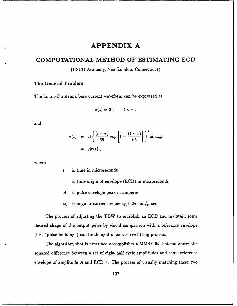
APPENDIX A

COMPUTATIONAL METHOD OF ESTIMATING ECD

(USCG Academy, New London, Connecticut)

The General Problem

The Loran-C antenna base current waveform can be expi-essed as

x(t) = o; t <r,

and

x(t) = A (t -T) exp I- (t ] }) sin Wot

= Ar(t) ,

wheret is time in microseconds

T is time origin of envelope (ECD) in microseconds

A is pulse envelope peak in amperes

wo is angular carrier frequency, 0.27r rad/ji sec

The process of adjusting the TDW to establish an ECD and maintain some

desired shape of the output pulse by visual comparison with a reference envelope

(i.e., "pulse building") can be thought of as a curve fitting process.

The algorithm that is described accomplishes a MMSE fit that minimize,, the

squared difference between a set of eight half cycle amplitudes and some reference

envelope of amplitude A and ECD r. The process of visually matching these two

137

data sets when expressed mathematically becomes a cost function, J. This squared

error then becomes8

J = ý[s(i)- A-(i]2i=1

where r(i) is the model which is a function of ECD. When J is minimized, this

constitutes a MMSE fit.

Minimization of the Cost Function, J

In order to minimize J we will use partial derivatives. For wel behaved Loran-

C pulses and quadratic cost function, there is only one global minimum, and no

maxima. Therefore we will set,0J

and

8A -0 .

Therefore,8

= Z[s(i) - Ar(i)]2i=1l

which impliest3J 8

-A 2[s(i) - Ar(i)j]-r(i)] = ,i=1

and

= _ 2[s(i) - Ar(i)] -ar(i) = 0 .

The solution for A is straightforward, yielding

8Z•s(i)r(i)

8

Er_2 (i)i--1

The solution for r is a bit tougher!

138

______________________________A

Quadratic Approach

s = Z[s(i) - Ar(i)12i--1

is called a quadratic cost function since for linear differences of [s(i) - Ar(i)], J is a

second order polynomial. Although [s(i) - Ar(i)] is not a linear difference function

of ECD, it becomes approximately linear in the region of minimum J for small

differences of ECD. This says

J - Jo = K(r - ro)2

where

Jo = minimum cost,

and

ro = the associated ECD at that Jo

Now let's choose three points for this function, separated by a common dis-

tance, J. This says

(J1 - Jo) = K(rN - r-o) 2 ; rT = N - 6

(J 2 - Jo) = K(T-N -- o)2 ; T = TN

(J 3 -Jo) = K(rN + -To) 2 ; rT= rN+b

Now we have three equations and three unknowns, so that the solutions are

J, - 2J2 + J3

6( J 1 - J3 )2(J 1 - 2J2 + J3)

and

Jo = J2- K(T - ro)2

139

However, the r0 above does not provide an exact solution to the minimum of

J. We'll need an iterative algorithm. This algorithm can be stated as follows:

,I (J3- J)k+1 = r- 2(J 1 - 2J 2 + J3)

a) Let initial ECD = 0, 61 1, compute J1, J2, J3 , r2

b) Let 62 = 0.1, compute J1, J 2, J3, r3

c) Let 3 = 0.01, compute J1, J2, J 3, r4

d) Let 63 = 0.001, compute J1, J2, J3, r5

rs represents the best estimate in the MMSE sense for the ECD.

140

APPENDIX B

DATA COLLECTION AND FORMATTING

The enclosed MATLAB programs describe how data vectors were collected and

formatted for this project. These programs format the original ASCII data vectors

and store them as vectors in eight sets in binary MAT-file form. This allows the

data to be loaded quickly and easily.

141

% SAV DAT: Corrects and formats Loran-C ASCII data files for use in% 9ATLAB & saves them in binary form in sets of manageable size.% In each set are several pairs of input and output vectors, labeledI xP and yP respectively, where P is the pair number, unique throughoutt all the sets. Each set is a single MAT file named datasetS.mat,W where S is the data set number. The variables may be loaded one

n set at a time or all at once using LORLOAD.W Calls: MAXVOLTS

t Data pairs available:3

i 31 July 91: 5 pairs for the 42 xmtr with antenna simulator1 06 Sept 91: 3 pairs for the 42 2amtr with antenna simulator

1 3 pairs for the 42 xmtr with dummy load% 28 Feb 92: 20 pairs for 42 xmtr w/ simulator1 20 pairs for 42 xmtr w/ dummy load%I (Note: this data set is subdivided as follows:1 22 May 92: 16 pairs: an entire GRI, compensated and uncompensatedI for droop (42 antenna simulator)1 30 Jun 92: 19 pairs (20, but pair 80 is actually 2 inputs)I for the '44A xmtr, with dunmy load, antenna sim.W & 625' monopole antenna (pairs 81-83 only areI on antenna)

I This program decimates each data vector to a desired samplingt frequency, using a lowpass filter to prevent aliasing. The zero! level of each data vector, estimated by taking the mean of the% last 596 sample points, is subtracted so that any DC measurementt bias is removed. Each data vector is normalized to 1 and thenI then scaled up to the correct voltage. Although the Loran-C outputI current is customarily measured, in this engineering model the outputI voltage is measured, using an infinite input impedance at thet oscilloscope. This is not the same as the voltage read by theI Electronic Pulse Analyzer (EPA). In cases of 6 Sept 91 and following,t the transmitter cathode current (TKI) was generally held at about 1.0I amp. All '42 rf vectors were measured from the J6 jack. The '42t rf vectors were measured from the J26 jack. For the :44A dummyt load data a 20 db attenuator was used (model 42, ser # 173-56)t since the J26 jack is uncalibrated and unloaded. If implementedI on the '44A this should really be buffered better.

I Dean C. Bruckner, 11/22/91 Rev. 9/4/92

clc;disp(' Caution: running this program will clear the workspace.');disp(' Press return to continue or ctrl-C to abort.');disp('');pauseclear

N1=[i 2 4 8];Nl indxumenu('Select Decimation factor','1','2','4','8');N-Nl(NIindx) ;disp(['N a ',num2str(N),' selected'])disp('Press <Enter> to continue or ctrl-C to abort'),pausefs-lOe6/N; len.4096/IN;

ptul[ 6 12 22 32 42 1 Data pair numbers in each set5 11 21 31 41 51];

142

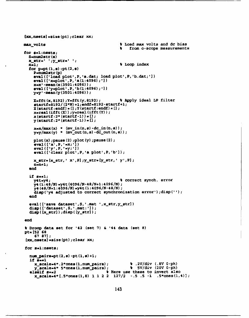
(xx,neetal -size (pt) ;clear xoc;

max-volts V Load max volts and dc bias!k from 0-scope measurements

for s-1:nse~ts;Sanum2str (a)x stral' ;Ystral ';

n-1; V Loop indexfor puapt(1, a) : pt (2,sa)

Panum2str (p)eval([load plot',P,'a.dat; load plotr,P,lb.dat;,1)eval( ('xnplot' ,P, 'a(1:4096); '1)zx' l-mean (x(3501:4096));eval(['y~plot',P,'b(l:4096);'1)yuy' -mean (y (3501:4096));

Xumfft(x,8192);Yunfft(y,8l92); V Apply ideal LP filterstartf-S192/ (2*N) +l;endf=8192-startf+l;X(utartf:endf)-t] ;Y(startf:endf)-Ul;xmreal (ifft (X)) ;ynreal (ifft (Y));x(utartf:2*(atartf-l))-[1;y(startf:2* (startf-l) ) = C;

xnx/max(x) * (my -in(n,s)-dc-in(n,s));yuy/max(y) * (my out (n, s) -dc out (11, ));

plot (x) ;pause (2) ;plot(y) ;pause (2);eval(['x',PD 'mx;'])eval(['y',P, '=y;':J)eval(I'clear plot',P,'a plot',P,'b']);

xustr-Ix~str,' x' ,P];y~stru Ly str,' y' ,P];n-nil;

end

if anal;y4tay4; t correct synch. errory4 (1:48/N) =y4t (4096/N-48/N+l :4096/N);y4 (48/N+1:4096/N) my4t (l:4096/N-48/N);disp('y4 adjusted to correct synchronization error');disp('');

end

evalU'seave dataset',S,' .mat ',x-str,ygstr])disp ( E dataset' ,S,' .mat:']);disp ( Ex...strl) ;disp ( Ey..str])

end

Ir Droop data set for '42 (set 7) & '44 data (set 8)ptw!52 68

67 87];[Joc,nasts] -size (pt) ;clear xx;

for s-1:nsets;

numapairsnpt (2,s) -pt(1, a) .1;if analx ucale=4*.2*ones(l~num...paira); t .2V/div (.8V 0-pk)y-scale=4* 5*ones(l,num..paira); * 5V/div (20V 0-pk)

elseif s--2 V Here use these to invert alsox-scalew4*C.S*oneu(l,8) 1 1 2 2 127/2 -.5 .5 -1 .5*ones(1,4)J;

143

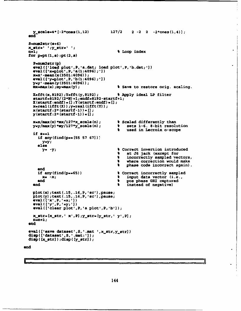
y-scalem4*1-2*ones(l,12) 127/2 2 -2 2 -2*oneB(l,4)];end

Sanum2str (s+6x stra' ';yustrm' ';n.-1; V Loop indexfor papt (1,.a) :pt (2, s)

Pmni- sutr (p)*val(E'load plot',P,'a.dat; load plot',P,'b.dat;'])eval(E'xmplot',P,'a(l:4096);'I)xax' -mean (x (3501:4096));eva3l(C'ymplot',P, Ub(l:4096);'])yny' -mean (y(3SO1 :4096));wmxmaxWx;irjmmax(y); * Save to restore orig. scaling.

Xafft(x,8l92);Yinfft(y,8192); * Apply ideal LP' filterstartf=8l92/ (2*3) +1;endfm8l92-startf+l;X(utartf:endf)mfl ;Y(stwxtf:endf)m U;i-real (ifft (X)) ;ymreal (ifft (Y));x(utartf:2*(startf-l))-[];

xax:/max (xl imx/127*x-scale (n); V Scaled differently thanymy/max(y)*my/l27*y-scale(n); V sets 1-6. B-bit resolution

if Bal used in Lecroix o-scope

if any(find(pan(55 57 67])%,y-y;

elsey- -y; V Correct invertion introduced

t at J6 Jack (except for%- incorrectly sampled vectors,t where correction would make

I phase code incorrect again).endif any(find(p.=65)) V Correct incorrectly sampledxu -x; t input data vector (i.e.,

end t poe phase GRI capturedand I instead of negative)

plot (xl ;text(.15, .16,5', 'c') ,pause;plot (y) ;text(.15, .16,5', 'c') ,paume;evalU'Ix',P, 'mx;'])eval( ['y,P, 'my;'])eval(E'clear plot',P,'a plot',P,'b']);

xmstr.[xý..str,' i' ,P'];ymstrmCystr.' y' ,P];n7.n+l;

end

eval(E'save dataset',S, ' .mat ',x-str,y-str])disp( C'dataset' ,S,' .mat:']);diep ( Cx utr) ;disp ( tyastri)

end

144

t MAX VOLTS: Measurements from oscilloscope plots for AN/FPN-42% Loran-C transmitter. Each value if the max positive valueI in volts. Called from SAV DAT. Data sets 7 and 8 weret formatted more directly and easily by just using the o-scope scalet instead of reading the plots. But since these were done alreadyI they stayed as is.

mv inozeros(10,nsets); W Max volts of input vectorsmy out-zeros(10,nsets); V Max volts of output vectorsdc-inuzeros(i0,nsets);dc-outmzeros (10,nsets);

mzyin(1:5,1). [.72 .74 .28 .28 .48]'; W (from o-scope plots)mv out(1:5,1)= [17.2 16.2 3.3 1.62 17.21';mv_-in(1:6,2)- [.82 .8 .93 .9 .52 .51]';mv out(l:6,2)- (24.5 8.2 27 10 3.0 1.2]';mv-in(:,3)w 2*[2 .85 .6 .55 .5 .9 3.3 2.3 1.8 1.35]';mv out(:,3)= -2*10*[1.55 1.45 1.15 1 .83 .5 .26 .22 .2 .27]';mv in(:,4)} 2*[4 4 2.75 .86 .75 .63 .46 .3 .32 .4]';mvyout(:,4)= -2*10-[1.4 1.37 1.5 1.37 1.29 1.2 .68 -1.3 -1.39 -1.65]';mv in(:,5)n 2*[2.4 1.05 .69 .61 .49 1.9 3.75 2.6 1.1 1.09]';mv out(:,5)- -2*10*[.49 .47 .39 .265 .22 .46 .14 .12 .135 .141]';mv_--in(:,6)- 2*[3.65 3.95 3.79 1.25 .9 .8 .79 .305 .36 .54]';nv-out(:,6)u -210*(.2 .46 .47 .46 .43 .38 .39 -. 4 -. 44 -. 53]';

t Corrections:% - Outputs accidentally inverted1 2 Correcting for differences in o-scope input impedanceI settings (50 ohm evenly divided voltage with theI load and so its amplitude was only half of thoseI taken with infinite input impedance. Thus they need

I to be doubled.t 10 A 1OX probe was apparently left out of these meas.

dc in(l,1)u .01; V DC voltage bias in measurements,dc-out(l:5,1)- [.1 0 .05 .02 0]'; V from plotsdc out(1:6,2)- [.5 .2 .2 .2 .05 0]';dc6in(:,3)- .01*[3 zeros(l,8) -11';dc out(:,3)- .01*[3 zeros(1,5) .5 0 0 0]';dcmin(:,4)- .01*[zeros(1,5) .5 0 1 1 1]';dc-out(:,4)a .01*[zeros(l,7) 1 2 2]';dc-in(:,5)- .01*[3 2 1 1 1 5 5 5 5 2]';dc-out(:,5) .01-[0 0 1 1 1.5 1 .5 .5 .5 .5]';dc-in(:,6). .01*[10 5 5 3 3 3 3 1 1 1]';dcout(:,6)m .01*[.5 1 1 1 1 1 1 2 1 i]';

145

[THIS PAGE INTENTIONALLY LEFT BLANK]

146

APPENDIX C

FITTED CURVES FOR CATENATED MODELS

This appendix contains fitted curves of magnitude and phase for the catenated

models, as follows. For values of E,, outside the endpoints of the curve, the function

simply assigns the value of the curve at the nearest endpoint. In the titles "A"

indicates the antenna and "D" the dummy load.

Transmitter Description Page

AN/FPN-42* 19-point curves for combined model, antenna 148simulator (4 poles, 3 zeros)

AN/FPN-42* 13-point curves for combined model, dummy 152load (2 poles, 1 zero)

AN/FPN-44AM 15-point curves for combined model, antenna 154simulator (6 poles, 5 zeros)

AN/FPN-44A° 4-point curves for combined model, dummy 160load (4 poles, 3 zeros)

AN/FPN-42 5-point curves for first catenated model, an- 164tenna simulator only (4 poles, 3 zeros)

" 4-part set of curves used in computer simulation program for N = 1.

147

CPLX POLE PAIR 1, '42 (A, N=1)Magnitude of Selected Parameter

0,9,, -q-,-,�r p y

Order - 60.999

�ggg -

I.

0.998 .A1LL J.0 5 10 15 20 25 30 35 40

Energy of normalized input vector, watt-gee X I e-6

PI'�age of Selected Parameter0.068 -,-r

0

0.066 �:0

0.067 -.--. &----**-

-- -- �.-..-.-.--- ,....,............4.**......-..*..

0.067 -

0.066 - & J a &0 5 10 ¶5 20 25 30 35 40

Energy of normalIzed Input vector, watt-eec X I e-6

148

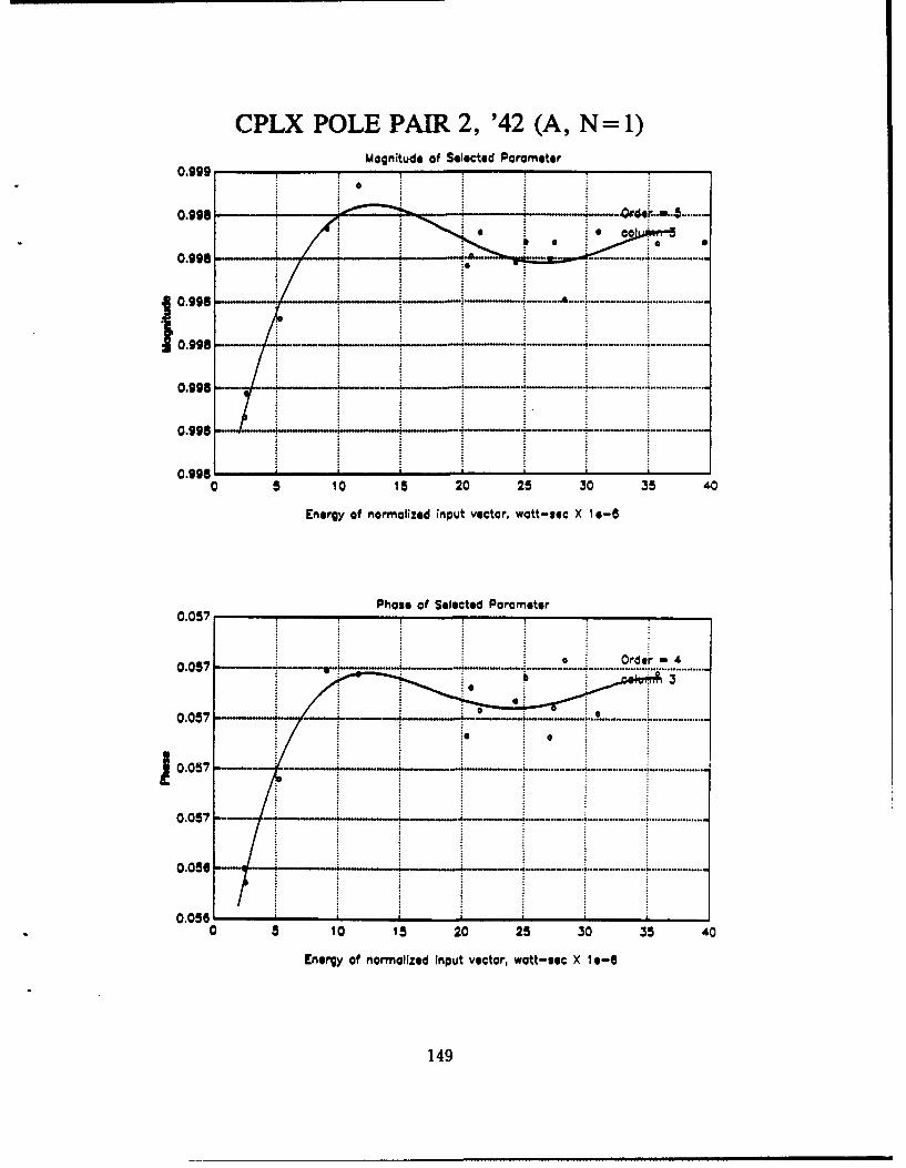
CPLX POLE PAIR 2, '42 (A, N=1)0.000 - ~ -~ Magnitude of Selected Parameter0.999

0.008 - '- - A.

a ----...- a ...-.---. ...-.-- ' . -.-. ............

0.008-.........

0.008 - '

0 5 10 15 20 25 30 35 40

Energy of normalized input vector, watt-see X Ic 6

Phase of Selected Parameter0.057 IYP

0 Order-43

0. 5 .......... .... ...................

0.057 ................- .

0 5 10 Is 20 25 30 35 40

Energy of normalized Input vector, watt-sac X Ic 6

149

CPLX ZERO PAIR, '42 (A,9 N=1)1.oa Magnitude of Selected Parameter

1.07

e ~colui m 5

1.05 - .---.-. - ----- ----

j 1.03 -

1.03 ----- --------- ..... . .......

0 0

1.01

1.01 ____9.

0 5 10 15 20 25 30 5

0.07

0.05 .....~.~ . . .... ............... ....m..........h

0.05

0.02 - 4--- -0 5 10 Is 20 25 30 35 4.0

Energy of normalized Ir ;ut vector, watt-sec X I e-f

150

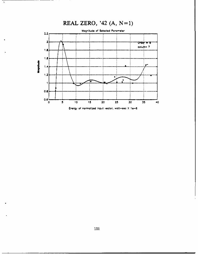
11IEA L Z ERO0, '4 2 (A, N =1)Magnitude of Selected Parameter

colum n 7

*1M

0.6

Energy of normalized input vector, watt-seec X Is-$

CPLX POLE PAIR, '42 (D, N=1)Magnitude of Selected Parameter

Order': 3

0.997- a.....

0 5 10 15 20 25 30 35 40 45

Energy of normalized input vector, watt-sec X 1. 6

Ph~ase of Selected Porameter

0.063

0 '0

0.060

0 5 10 15 20 25 30 35 40 45

Energy of norrmalized Input vector, watt-sec X Is-$

152

RXCEUAL ZERO, '42 (D, N =1)Magnitude of Selected Porarmeter

1.0.

1.035 ....* .-..........-* *.*.... Ore : m..4.....

* . . .colur~ni 3

..2 -- . ... . .... ...... ......... .... .. ot

1.005 ~& .0 5 10 15 20 25 30 35 40 45

Energy of normalized input vector, watt-soc X lo-8

153

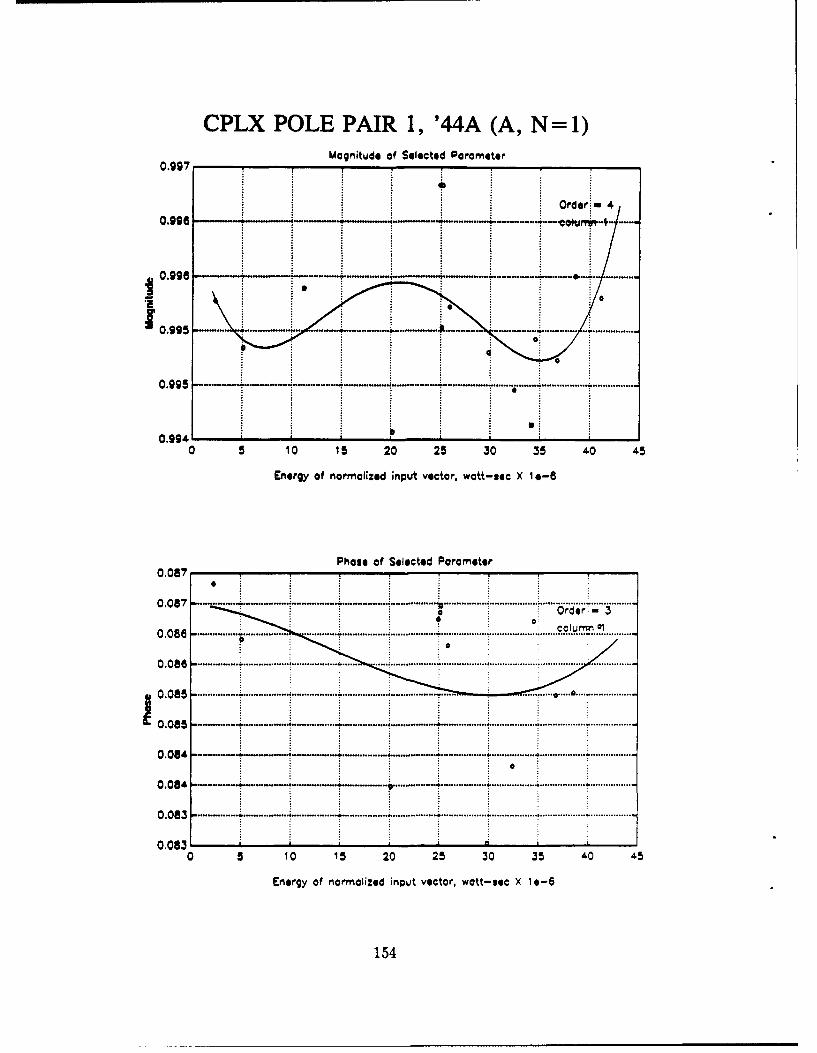
CPLX POLE PAIR 1,ý '44A (A, N =1)Magnitude of Selected Parameter

0.997 - - - -

Order - 4

b 00

0 5 10 15 20 25 30 35 40 45

Energy of normalized input vectar, watt-see X I a-8

Phase of Selected Parameter0,05

..... .*. ... . .m .. . ... . ... ..... ....... . . . . . . . . . . . .

0.08*a*...8.................. .....................

0.085 .. ....... *.... ............

0...........0.2....0.....0 . 4.

0.01134

CPLX POLE PAIR 2, '44A (A, N =1)Magnitude of Selected Pararmeter

Order: 5column 3

0.2999 -. . - -- -- ' .. ..-............... ..................e.........

0O.9 9 9

.... ................. .........

0.999,

0 5 0 15 20 25 30 35 40 45

Energy of normalized Input vector, watt-seec X 1 e-8

Ph~ase of Selected Parameter0.066 --

. ... ....... ............ ......... 1c '11 .im

column~ 3

00 . ......... . . . . ............ . ..... .... ....

0.065 ....... ......... .............-..... ........

0.045 F L L _ _ _ _ _ _ .......... ..........

0 5 10 15 2n 25 30 35 40 45

Energy of normalized Input vector, watt-seec X 1 e-6

155

CPLX POLE PAIR 3, '44A (A, N= 1).9g9-tudo of Selected Parameter

* Order:: 3

8 0.995. . . ..

0.994 ...... ............ ......... . ..........

I,

0.994. ,.,.,

0 5 10 15 20 25 30 35 40 45

Energy of normalized input vector, watt-sec X le-6

Phase of Selected Parameter0,046 ,

0.046 ............ . . .. ........................ ............. ................... .................. ..................................... ....................Ordor; - 2

0.045 " . -............. .olrn 50. 4 . . .. . .. . .. ...... .... ..... ..................................... .................... ................... ................... r.................

0.045 ..... .. ........................ ... ........ .. .....................................................

0,044 ................................... ........................

0 o,0 4 ............. .... ........... ...... ................... .............. *.... ................. .

0.04,4 .... .... ... ........... ...... .. ............... . .................. .• .................. ................... ................... .................

0.043 .. . . . .,- .... .. .. ..... • . .. ... +............... ................... ................... ................... •...•.............

0.043 .. ... . ........... ....... ............................................................

0.042 . . . . . . .

0 5 10 15 20 25 30 35 40 45

Energy of normalized Input vector, watt-$ec X le-6

156

CPLX ZERO PAIR 1,ý '44A (A, N=1)Magnitude of Selected Parameter

1.02 r,

~~~~~.................... ........... .............0ae.. .........3

1.005 ...

0.960

0 5 10 15 20 25 30 35 40 45

Energy of normalized input vector, watt-soe X 1e-8

Phase of Selected Para meter0.115

0

Order:: 4

* colur* 7

1 0.015 ...................

0.080

0 5 10 15 20 25 30 35 40 45

Energy of normalized input vector, watt-sec X le-6

15~7

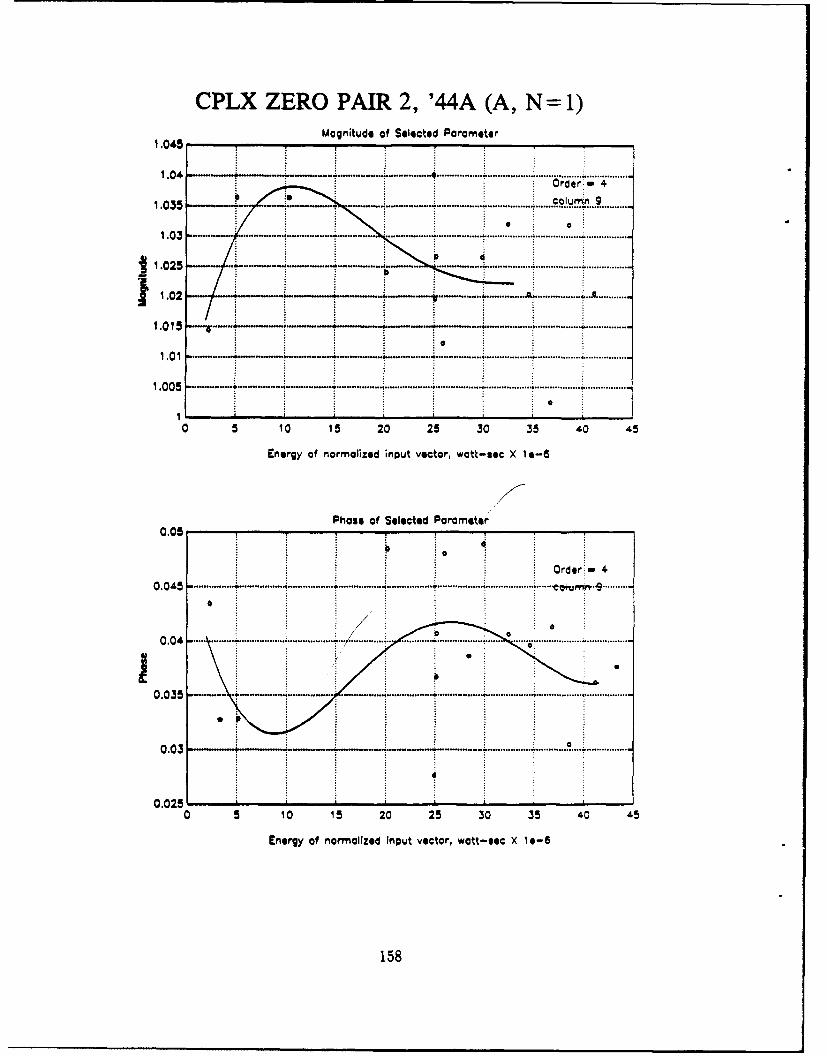
CPLX ZERO PAIR 2,9 '44A (A, N =1)Magnitude of Selected Parameter

1 .045 - - ' '

1.04 "---.-. . .-- -. ............... . ...... .......... . ........................-........Order.= 4

0

0.015 . ........... ..... ........

0.041 ....................

0 5 10 15 20 25 30 35 40 45

Energy of normalized input vector, watt-sec X 1e 6

0.158

REA ZRO '44A (A, N=1)Magnitude of Selected Parameter

1.03

colurrw, 11

1.01 ~.......................................................

0.96 1

0 5 10 15 20 25 30 35 40 45

Energy of norrmalized input vector, watt-see X 1 e 6

159

CPLX POLE PAIR 1, '44A (D, N 1)Magnitude of Selected Param~eter

0.997 y1 ~

co rm 10.997 -. . - - - ' . - - ...'.................... .......... .......... .........

0.997 .....~ .......- ...... ...... . ....

10.997 .1.......... .. .......... .........

0.997------

0 5 10 15 20 25 30 35 40

Energy of normalized input ýector, watt-see X le-6

Phase of Selected Parameter0.069 - v

Order - 3

0.069 ..-- . ... ... ...............................

0.069 -........................ . . . . . . .

0.069 *-.................. ..

0 a 10 15 20 25 30 35 40

Energy of normalized Input vector, watt-sec X Ise-$

160

CPLX POLE PAIR 2,J '44A (D, N 1)Magnitude of Selected Parameter

0.99 -~Order - 3- columrn 3

-.------~ - ----- ..................................-.........

10998 .~. ...... ...........................

0.907 ------ ..........

0.997 - - . - ...........-......... ....................

0.997 h________

0 5 10 15 20 25 30 35 40

Energy of normalized input vector, watt-see X I e-6

Ph~ase of Selected Poarameter0.061 - -

ordqr- 3

0.06 ---.... .--..... Colunrri 3

I 0.061 .. . . ~ . . .. ..... ..............................

0.06 - i - .- --. .--. .. .......- .............. .. .........

0.06

0.06 ...... ~____ --. .-.

0.06 - .

0 5 1 0 15 20 25 30 35 40

Energy of normalized Input vector, watt-sac X( is-6

161

CPLX ZERO PAIR 1,ý '44A (D, N =1)0.989Magnituds of Selected Parameter

0.989 ... -... ......

0.988 - ... . .. . ......... ... ..........

0.988 6

0 5 10 15 20 25 30 35 40

Energy of normalized input vector, watt-sec X I e-6

Phase of Selected Parameter0.07 r9

0.07Order -3Colurrin 5

0089 .. -.. - . . . . ................ .....................................

0.06 9 .......... ......... 4 ......... ............ ....i.. ................ .......................

0.06 F

0 5 10 15 20 25 30 35 '0

Energy of normalized input vector, watt-sec x Is e6

162

REAL ZERO, '44A (D, N= 1)Magnitude of Selected Parameter

0,991

0.99 ----.-. Order 30.99 ---- --- - :...... ........................................ ..................................... .•.•.... ... ...........Coi~nmn 7

.. .. ... 8 ..... .. .. .......... .... '.... ................. •.... ................. •..... .. . . . . . .

0 .98 7 ..... ... . .. . .. .......... ..... ..................... ....................

0.986 ..... .... ........... A ...................

0.285 "0 5 10 15 20 25 30 35 40

Energy of normalized input vector, watt-eec X le-S

163

CPLX POLE PAIR 1, '42 (A, N = 1 5 PAIRS)Magnitude of Selected Parameter

0.998 3

0.998 - ... ................................ .................. .. Qa... m ....A

0.998 -- .-.- . - .- -.- .. . .. ... ................. ........

0.998

0 5 10 15 20 25 30 35 40 45

Energy of normalized input vector, watt-sec X 10-6

Phasge of Selected Parameter0.066 8

Order:

colu I

0.067 .... .... ....... .....

0.067

0 5 10 15 20 25 30 35 40 45

Energy of normalized Input vector, watt-3eC X 1Is-$

164

CPLX POLE PAIR 2,9 '42 (A, N =1, 5 PAIRS)Magnitude of Selected Parcrmetor

0.999

columln 3

0.999 .. .-.- .- ...... ................... ..... ........

1 0.99a8.. . .. .......... ........

0.998 . 6 ..

0 5 10 15 20) 25 30 35 40 45

Energy of normalized input vector, watt-94e X le-6

Phase of Selected Pacrometer0.057 -

0.57Order 4

0.057 .......- - -..... -......... ....... .......... ........... 4......... .......... .... ................

I 0.057 -.. . . . . ............ ......... ......................................

0.057 / ....-.---- -- ------------------ ........

0.057 .

0 5 10 15 20 25 30 35 40 '5

Energy of norrmalizd Input vector, watt-sec X le-6

165

CPLX ZERO PAIR, '42 (A, N =1, 5 PAIRS)Magnitude of Selected Paramneter

1.07-

1.06 -.................. ......... .... . ...Q., ... .

column

.9 1.04 ....... ................ .........

1.02 .. .. ...........

0 5 10 15 20 25 30 35 4-0 45

Energy of normalized input vector, watt-sec X 1e-6

PhaSe Of Selected Pa~rameter

0.08 .. . -

Orogr -4

0.07 . ..................... ............................- .

00 . . .. ......................... ............... ......

0.01 4 .................. ............................

0 5 10 15 20 25 30 35 40 45

Energy of nornmalized Input vector, watt-sec X le-6

i 66

REAL ZERO, '42 (A, N= 1, 5 PAIRS)-agnitudof Selected Paometer

1.35 ,.,.

1.25 ........ ....... ............... ................... -r............. ........i i i ii ! olu• 7

12 ..-.. . -.. .. - . . . ... ....... .. .............. .........1.25 ...... ."• • .. . ... • . .. .. .. ........... ... •................ "•........... ..... .................

1. 15. ... ." ... .. . ; ...... ..... ". ....... .." ................ .. . .............. ................... ....... ......... ................. .

S1 1 . .. ...." .............. .... ........ .: . ............... .................. : .................. • ..................... ............... . ................ .

1.0 .................-. .... ....... ..... 6 ............... -. .................. i .................. ................... •.. .......... .... ... .................. ,. .................

1.05 -... . . . ....

0.950 5 10 15 20 25 30 35 40 45

Energy of normalized input vector, watt-seec X 1e-6

167

[THIS PAGE INTENTIONALLY LEFT BLANK]

168

APPENDIX DSELECTED MATLAB PROGRAM LISTING

The following MATLAB M-files are part of the simulation program. The main file

is SIMZ, which calls more than fifty functions in the course of a simulation run.

Space does not permit a full listing here. The last function listed, MODELYW,

was used for modeling and is not directly part of the simulation program.

169

% SINZ: Simulates controlling the AN/FPN-42 and 44A Loran-C% transmitters in the z domain.% Calls SETUP, AR2, XMTR, INTERP, ERRORS, PULSINI, MAINMENU,

FINDPSV, ENVEL, DISPZI and the function defined in 'fcall' (see SETUP).% Also calls file named in row string matrix ALGSWP (See SETUP)

t Dean C. Bruckner, 4/12/92, rev. 9/12/92

* * Initialize program *

clearsetup I Declare vars & intializefirst run='y';done simz='n';mainmenu I First menu (see end of loop

t for other occurrence)while done simz=='n'

* * Enter control loop *

for p=l:length(control);

if pm=l;num_iter-numiterl;else numiter=numiter2;endV If drift will be used, start with nonzero random drift vectorI if first run.if drift iter~=O & first_run=='y';

(driftdriftstor]=ar2(drift-stor,step);end

PSTR=['Pulse ',num2str(control(p))];PC=phasecode(control(p));tdw=tdwp_1ci(:,p); V Select one input pulsepuls_ini V Initialize pulse convergence

V plot and misc error matricesI for this loop only.

donejpulse='n';m=l;md=l;ms=l;tO=clock;while done-pulse=='n'

if m>l;times(m)=etime(clock,tO);endt0=clock;M=num2str(m);Ml=num2str(m-1);

V *********** Find restl for GRI of subject pulse *

restl=rests(rest_indx); V Rest time for pulse 1 of GRI

blank=blanks(restindx); t l=rate blanked in this iter.W O=rate not blanked.

rest indx=rest indx+T_dso/ratel; V Find rest indx for next time.while restindxilength(rests)-I t Wrap index around

restindx=restindx-length(rests)+2;end;

if m<5 & err disp=-l;plot(tdw);pause;end

if blank-l;

170

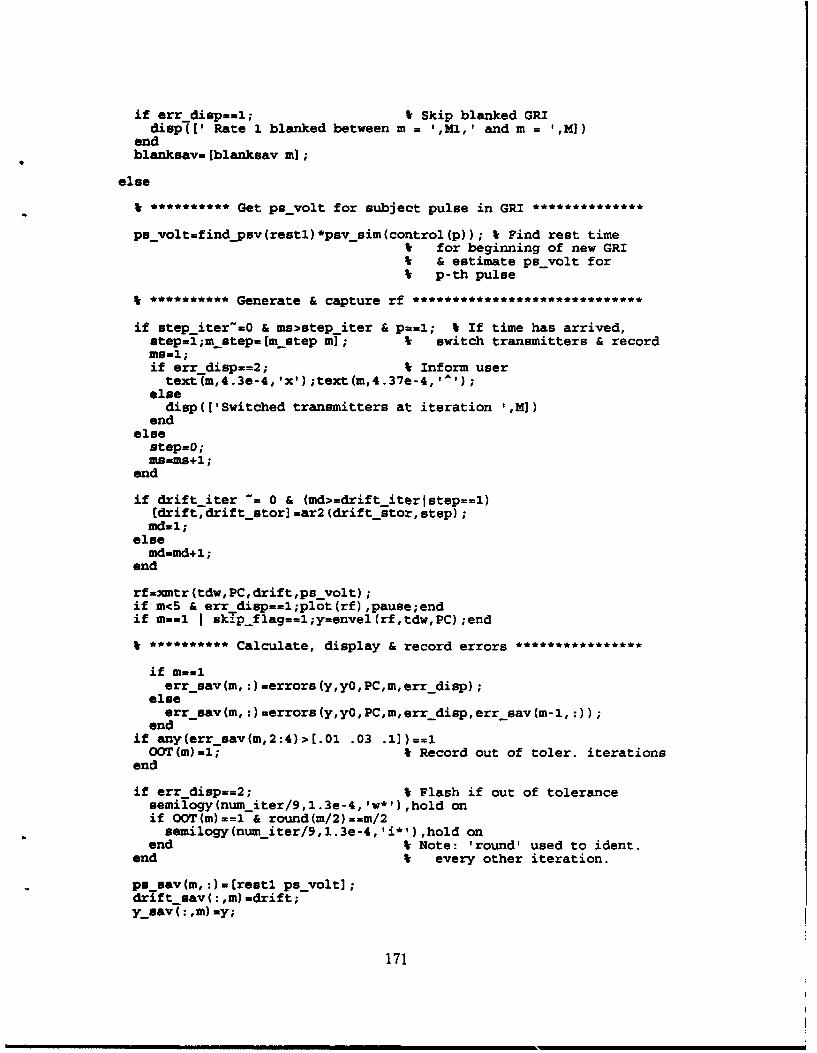
if err disp-.i; * Skip blanked GRIdisp(C' Rate I blanked between m = 1,M1,1 and m

endblanksavz (blanksav ml;

else

V***** Get ps volt for subject pulse in GRI

ps-voltafindpsv(restl)*psv-sim(control(p)); V Find rest timeIr for beginning of new GRI

' & estimate p. volt forIs p-th pulse

~~ Generate & capture rf

if step_iter=0O & ms>step iter & pm=l; * If time has arrived,stepml;m step=uvm step in]; $k switch transmitters & recordms=l;if err -diSp==2; t Inform user

text (m,4.3e-4, xl ;text (m,4.37e-4, A')else

disp(I'Switched transmitters at iteration 1,M])end

elsestep=0;ms=ms+l;

end

if drift iter -a 0 & (md>=drift iterlstep==l)(drift7,drift-stor]=ar2(d~rift-'stor,step);mdul;

elsemd-md+l;

end

rf=nwitr(tdw,PC,drift,ps-volt);if m<5 & err disp==l;plot(rf),pause;endif mm== I sk~ip~flagm~l;y-envel(rf,tdw,PC);end

V Calculate, display & record errors

if mu=lerr sav(m, :)=errors(y,yO,PC,m,err-disp);

elseerr-sav(m, :)-errors(y,yO,PC,m,err-disp,err-sav(m-l,:));

endif any(err-sav(m,2:4)>[.0l .03 .l])1=OOT(m)=l; t Record out of toler. iterations

end

if err dispw=2; V Flash if out of tolerancesemiiogy(num -iter/9,l.3e-4, v*1) ,hold onif OOT(m)m=l & round(m/2)==m/2

uemilogy(num-iter/9,l.3e-4,Ii*'),hold onend t Note: 'round' used to ident.

end t every other iteration.

puusav(m, :)-[restl ps -volt];drift sav(:,m) -drift;yusav( ,m) my;

171

%snrtdw(m)-snr(tdw); V record SNRs for averaging

%snr rf(m)-snr(rf); V Note: change DISPZ also

t Produce new tdw *

eval (f-call)

I ********** Fill AFG buffer with new inputs *************

for ppap:length(control) I (pth & following pulses)

t If in GRI A, boost each following tdw in GRI A so when it isI controlled, convergence will be faster. Undo the phasecodet of each pulse & then reapply it as appropriate. Variablet "boost" is set in **** INI, not in XMTR CFG (since knowledget of needed boosts should be experimentally obtained).% To boost the tdws in GRI B when controlling a pulse in GRI A,t scale back to pulse 1 in GRI A and then skip to GRI B, scalingt up from the first pulse in GRI B.t If in GRI B, do the same.

if control(pp)<=lenp/2; t both in GRI Atdw-pci (: ,pp) boostA (control (pp) -control (p)) *...

(tdw* (-1) APC) * (-l) Aphasecode (control (pp));elseif control(p)<-lenp/2 * in different GRIs

tdwpci (:,pp)mboostA(l-control (p))*...boostA (control (pp) :lenp/2-i) *...(tdw* (-l) APC) * (-1) phasecode (control (pp));

else V both in GRI Btdw-pci (: ,pp) =boostA (control (pp) -control (p))*...

(tdw*(-l)APC)*(-l)Aphasecode(control(pp));end

end

t ********* Swap XMTR loads if error below threshold *

if xmtrload=='Dtumny Load' & all(errsav(m,2:4)< [.006 .015 .05])==1in_swp=m;xntr load = 'Antenna '; t Change to antennaeval(algswp(alg,:)) t Reset part of algorithmif err disp=-2; t Inform usertext (m,4.3e-4, 'a ) ;text (m,4.37e-4, ' ') ;else

dispU'Switched to antenna after iteration ',M])endskip flagul;

end

mwm+l;

end t end 1 iteration

if m>nminu_iter+l;donepulse-'y';end

end t end 1 pulse

t* Save rf and display results for pth pulse *

rf-pci (: ,p) =rf;if errdisp==2

172

text(.47,.2,'Press <Enter> to continue','sc'),pausehold off

elsedisp('Press <Enter> to continue'),pause

end

if any(control (p) uzanalyze) -l;dispz;endend % end 1 simulation run (all puls)first run='n';mainmenu % get new parameters for more runsend % end all runs & leave SIMZ

t SETUP: Sets up workspace for Loran-C simulation file SIMZ.t Declares global variables and assigns values to them. Sets upt workspace format and declares default settings such aa the typeV of random number distribution, etc. When user selects a controlt method a script file is used to initialize only those control% variables for the selected algorithm, including the controlI function call in a text string. Note that when a default settingV is changed here, it should also be changed in MAINMENU. Ift an algorithm is added, review MAINMENU carefully to ensuret parallel changes are made properly.t Calls PGEN, FLIPLR, ENVEL, and files named in string matrix ALGINIt ... COEFFSAV.MAT (created by MODlFMT1), HSCRPT, EOUT_EIN.MAT,t Declares all global variables used in this simulation.

* For complete list of variables see INDEX.

t Dean C. Bruckner, 4/22/92, rev. 9/2/92

format compactformat shortrand( 'normal')clc;disp('Initializing ... ')

t *** *** INITIALIZE TRANSMITTER MODEL ***** *

t **************** Declare global variables

global phasecode ratel rate2 staidglobal coeff bound rootindx psid cp cn cc crglobal drift sdev driftref ar2_var ar2 a ztoler ztimesglobal eout ein pstau psprev psimp p mindx N fs fs adjustglobal xmtr-id xmtrload bits imbalance signoise y0D-y0A tdwnoise

t ***** * Set up dual rate parameters

load restvars t Load variables for dual-rateV simulation (rests, staid,t ratel, rate2)

T dso=4; t Interval at which rf pulsesI are sampled by the digitalt storing oscilloscope (secs)

rsmrand('dist') ;rand('uniform') trest indx=round(rand*.9*length(rests)); V Start rest times index randomly.rand (rs)

173

**************** Set up Pulse measurement parameters

ztimes=(-25:5:30)'*le3; V Zero crossing times (ns)stoler-[ 2000 1500 1000 500 250 0 100 100 100 100 100 100

1000 100 75 50 50 0 50 50 50 50 50 50]';% These correspond to the category 2 & 1 xmtrs in the Loran signal spec.* The '42 is a cat. 2 xmtr; the '44A is catl (Note that xmtrid ist opposite from this: xmtrid=l is for the '42; xntrid=2 is the '44A)

I *Configure transmitter

xmtr idul; t 1 = 42, 2 = 44Axmtrload='Dummv Load'; V Starting load of xmtr,

I 'Antenna ' orW 'Dummy Load' (note: stringV lengths must be equal!!)

if sta id(l)=='S'; V Phasecode: 0=pos, l=negphasecode=[0 0 0 0 1 1 0 0 1 0 1 0 0 1 1'];

elsephasecode=[0 0 1 1 0 1 0 1 0 0 1 1 0 0 000 1'];

endlen_pmlength(phasecode);imbalance-0; V [0-100]; pct. by which the ampl.

I of neg. phase coded pulses is% decreased.

S** Load curves of xmtr model

N-l; * Default decimation factorxmtrcfg I Configure transmitter

* * Set up parameters for simulation

skip flag=0; V Used in switching automatically% from dummy load from antenna

control=l; t Pulses to controlanalyze=l; t Pulses to analyze (after

t convergence)tau=O; t Assigned local ECDETA-0; k Early timing adjust in

t microsecs (used in PGEN)bits=8; * Function generator resolution

1 ('0' selects best floatingt point resol. of the computer)

numiterl=100; V Iterations of 1st selected pulsenumiter2=20; V Iterations of following pulsesstep iter=0; V Interval between xmtr steps

t (switches)err disp-2; V Method of displaying errors

t during convergenceV 0-none,ltext,2=plot

V * INITIALIZE CONTROL ALGORITHM *

algal; k Default algorithm to start

t The following 5 string matrices are used to handle the currentt algorithm without listing the names of the algorithms or theirV associated files anywhere else in the program than here. The firstT string matrix holds the names of the algorithms; the following 4

174

% matrices hold names of files associated with each algorithm whicht are called at different points in the program. Lines 2 and followingt of each matrix should be the same length as line 1 and should follow"V suit.t Example:I alg-name='Steepest Descent ';I 'Neural Network ';V 'Recursive LS ';t The Steepest Descent Algorithm uses 6 modular M-files:I DESC The functionW DESC INI Initializes the algorithm% DESCNENU Lets the user change parameters easilyt DESCHEAD Menu header for DESCMENU* DESC SWP Resets part of the algorithm when xmtr load is swapped* DESCDISP Displays alg params for most recent run in DISPZ4 Other algorithms should use the same file structure. Details of thet minimum requirements for each of the above files are listed in theV text of each file.

alginame= ['Steepest Descent ']; k Algorithm namesalg-menu=['descmenu']; t M-file namesalgmýwp =['desc swp']; I "alg-ini =[ ['deuc-ii']; I ,algdisp=['descdisp']; "

eval(alg-ini(alg,:)) V Initialize algorithm

function rf=xmtr(tdw, PC,drift,ps volt)

t Function rf=XMTR(tdw,PC,drift,ps volt): Simulates the AN/FPN-42V or AN/FPN-44A Loran C transmitter. To account for nonlinearities,t the poles & zeros of the xmtr's transfer function are modeledV as a function of the normalized power supply voltage and thet energy of the normalized input waveform.V Uses global variables: bits, imbalance, sig_noise, xmtrload! Calls: ENERGY, FIND AB, FIND PSV

t Local variables:! A Amplitude of output vector (volts)% a,b Denominator & numerator polynomials of model% cr Number of rows in 'coeff'I drift Parameter vector modeling xmtr driftt energy_in Energy of input vector (watt-sec); R=1.t energy_no Energy of normalized input vector (watt-sec); R=1.t h Transmitter impulse response sequencet lc Slope & intercept of energy in/out of xmtrt psavolt Estimated normalized power supply voltage: (0,1]t restl Power supply recovery time since last pulset tdw Transmitter drive waveformt xmtrload String: Defines load connected to xmtr:t 'A'=antenna, 'D'=dummy loadt rf (Radio freq) output pulse

t Dean C. Bruckner, 7/17/92, rev. 9/7/92

I ***** Obtain xmtr transfer function *

175

if nargin<4;ps volt=l;end V Default: fully recoveredif nargin<3;driftmzeros(cr,l);end V Default: no driftif nargin<2;PC=O;end V Default: pos phase code

lentdwulength(tdw); * Length of input vector(energyin,energy no] =energy(tdw); V Energy of input vector

t (regular & normalized)

(a,b]-find.abl(energynops-volt,drift); t Denom & num polynomials

* * Produce output *

rfufilter(b',a',tdw);

* * Adjust output *************************************

if xmtr load--'Dummy Load'; t Apply input energy vs outputlc-eout_ein(2,:); W energy to find output

else W amplitude.lczeoutein(1,:);

endenergy out.lc(l)*energyin + lc(2);rf-rf/max(rf); V Normalize output sequence &A~sqrt(energyout/((rf'*rf)*N*100e-9)); I calculate final normalization

I power (power norm. to R=1)rfuA*rf*ps volt; * Assign estimated output energy

! to output sequence, includingI power supply droop.

rf-rf-mean(rf); 4 Remove DC bias

I Note on tube xmtr imbalance:t Initially the xmtr imbalance (between the 2 banks of tubes whichV amplify the positive & negative parts of the pulse, respectively)I was modeled in detail, as shown below, by adding up to one percentV distortion to the positive samples.%rf(•ind(rf>o))=(l-.Ol*imbalance) * rf(find(rf>O)); V xmtr imbalanceV Apparently this is an accurate representation of the distortion.! However, I could not find real documentation on the phase codeI balance adjustment that described exactly how this was remedied,t just that the imbalance caused negatively phase coded pulses toV be smaller in amplitude (both pos & negative parts equally), ast described in LCDR Taggart's EERP & VXIbus reports. According toI him, the phase code balance adjustment simply increases the amplitudesI of the TDWs for the negatively phase coded pulses, not adding anyt DC bias level, etc. Therefore, the imbalance is now modeledt as a percentage decrease in the amplitude of rf. This willt be compensated for automatically just like droop, since each pulset of the PCI is controlled independently.

if PC=W1; t For negatively phase codedrf=rf*(l-.Ol*imbalance); t pulses, decrease amplitude

end t by a percentage.

if signoise.O t Misc white noise in outputrs-rand('dist');rand('normal') t (std dev expressed as

t percentage of peak ampi.)rf.rf + .01*signoise*max(rf)*rand(length(rf),l);rand(rs);

end

if bits -. 0; t Amplitude resolution in DSO

176

max rf-max(rf);rf-round(rf/max_rf*(2*bits)/2) / (2^bits)*2*maxrf;

end

function tdwzpgen (x, PC, ETA);

% Function tdw=PGEN(x,PC,ETA): Simulates analog pulse generator,W given a 16-element vector of peak voltage values (pos & negt or all pos). Pulse is triggered 10 us after beginning oft data vector. Due to the problems of dealing with fractionalt values of samples per period, tdw is formed at 5.0 MHz and% decimated down to the desired sampling frequency.t Calls global variables: bits, xmtrid, fs

t Variables:t ETA Early timing adjust, in microsecs. Changes phaset of tdw within window (pulse still begins exactlyt at the trigger--ref. discussion w/ LCDR G. KmiecikI on 5/22/92). The effect of the ETA shows up inI the Envelope-to-Cycle-Difference (ECD) of the output.I fs_pg Sampling frequency used to build tdwI lenpg Number of samples in tdw at fspgI PC TDW phase code (O=pos, l=neg)t seta Number of samples in ETAI spp Samples per period (period = 10 us)I tdw Transmitter drive waveformV x 16-element input vector of pk voltage valuesI (pos & neg or all pos)

V Dean C. Bruckner, 2/21/92, rev. 9/7/92

t ******************* Verify inputs *******************************

if N>=2fspg=5e6;lenpg=2048; t 5 MHz has a whole number of

V samples in each half-cycle.else

fspg=fs ; lenpg=4096;end

if narginc3 ;ETA=0 ;endif nargin<c2;PC=0; V Check phase codeelseif PC~=0 & PC'-l;error('Phase code must equal 0 or 1');endif nargin<1;xwones(16,1); t Default: all 1/2 cycles equalelseif size(x)--[1,16];x=x'; V Reorient if necessaryend

if size(x)=[16,1] ;error('Size of x incorrect') ;endxmabs (x);

% *** * Generate PGEN input vector *

s eta=round (ETA*le-C*fspg);opp=l0e-6*fspg;k. (1: 8*spp) I;

177

m=ones(spp/2,1)*xI; t Extend vector x to each "bin"m-reshape(m,round(8*spp),l); V which is mult. by tdw

tdw(l:spp,1)-zeros(spp,1); W Trigger pulse at 10 us pointtempl=sin(2*pi*k/spp - pi*PC).*m; V Generate sine pulsetempi(length(tempi)-s eta+l:length(templ))=[]; t Apply ETAtemp2=-flipud(templ(1:-s_eta));tdw(spp+l:9*spp)=[temp2;templ]; W Recombineif xmtr id-=2

nn=2:lenpg-9*spp; I Tail drive circuittdw(9*spp+l:lenpg) mx(16) *...

(exp( (- (le6*nn/fs_pg)/22)) .*sin(.2*pi*le6*nn/fspg-pi*PC)) ';elue

tdw(9*spp+l:len_pg) =zeros (len pg-9*spp, 1);end

if N>2tdwmtdw(l:round(fspg/fs) :lenpg); t Decimate (ignore aliasing)

end

if bits =-0; V Amplitude resolution in AFGmax tdw-max(tdw);tdwvround(tdw/maxtdw*(2*bits)/2) / (2Wbits)*2*maxtdw;

end

if signoise=-0 V Misc white noise in inputrszrand('dist');rand('normal') W (std dev expressed as a

V percentage of peak amplitude)tdw-tdw + .01*tdwnoise*signoise*max(tdw) *rand(length(tdw) ,1);rand(rs);

end

function ps-volt=findpsv (rest1)

k Function ps volt-FINDPSV(restl): Given the time the xmtr powerV supply has had to recover from the last pulse of the precedingt GRI, this function estimates the new power supply voltaget (norialized and in the range (0,1]) for pulse 1 in the new GRI.V Uses global vars: pstau psprev ps_impV Calls:

* Variables:I ps-volt Estimated normalized power supply voltage: (0,1]t restl Power supply recovery time since last pulse

W Dean C. Bruckner, 7/20/92, rev. 9/7/92

if restl<.001;error('restl must be >= .001 sec.');endt--ps_tau*log(1-(ps_prev-ps imp)); V Point on the curve where

t recovery starts at end oft last GRI (note: "log" isV the natural logarithm)

ps-volt-l-exp(-(t+restl)/pstau); V psvolt after resting "restl"t seconds

178

function [a,b,h~yw]=model~yw(h,p,q)

P6Function [a,b,h~yw]=MODEL_YW(h,p,q): Solves Yule-Walker equations toP6find pole-zero model of Loran-C data vector.

V6 Dean C. Bruckner, 4/7/92. Adapted from algorithms written byP6 Tom Johnson of the Naval Postgraduate School.P6 Ref: C. W. Therrien, Discrete Signal Proc. & Statistical Signal

t6 Processing, Prentice-Hall, 1992.

len-halength(h);kx=lorcorr(h); t6 Autocorrelation vector by fftsRntoeplitz(Rx(l:len -h),Rx(l:p+l)); V6 ACF mtxRe=R(q+2:len-h,:); V6 Extended corr mtx (Ther. 9-168)

Ere, ce] =size (Re) ;a=[l;-Re(:,2:ce)\Re(:,l)]; P6 using extended Y-W method

P6 Note: Matrix pinv calculatedP6 by gaussian elimination.

ha=filter(l,a,[l;zeros(len h-1,1)J); V6 Use Shank's method toHa=toeplitz (ha, Eha(1) ,zeros(l,q)]); V6 find "b" parameters.b=inv(Ha'*Ha)*hal*h; V6 (Therrien ch. 9)

h_.yw=filter(b,a,[l;zeros(len-h-li1)]); P6 ARNA model impulse resp.

disp('Poles: ');

(abs (roots (a)) angle (roots (a))]disp('Zeros: ');

(abs (roots (1)) angle (roots (b))]d~isp('Press <Enter> to show plots');pause

cigif q>O;rts -b=roots(b); rts-b=rts-b(find( abs(rts-b)<2))polar(angle(rts -b) ,abs(rts -b), 'go') ;hold on;end;polar(angle (roots (a)) ,a~bs(roots(a)), 'rx');grid;title('Pole/zero plot of the Yule-Walker estimate');pausehold off

grid;title('Original & modeled sequence')xlabel( 'Sample number') ;ylabel ('Magnitude')text(.5,.15,f'145E = l,num2str(mse(h,h~yv)*le6),'e-6'],'sc')pause

179

[THIS PAGE INTENTIONALLY LEFT BLANK]

180

REFERENCES

1. Specification of the Transmitted Loran-C Signal, USCG Commandant Instruc-tion M16562.4, July, 1981.

2. Malcolm F. Willoughby, "The Story of LORAN," Chapter 10 of The U.S.Coast Guard in World War II, 1989.

3. Loran-C Engineering Course Manual, USCG Academy.

4. Bonnie Dahl, The Loran-C User's Guide, Richardsons' Marine Publishing Inc.,Steamwood, IL, 1986.

5. Gordon West, "The Electronic Radionavigation Plan," Trailer Boats, January1988.

6. Federal Radionavigation Plan, 1988.

7. Doug Taggart and Ben Stewart, "Electronics Equipment Replacement Project(EERP)," Technical Report, USCG Electronics Engineering Center, 1989.

8. Loran-C Engineering Course Reference Manual, USCG Academy, 1988.

9. Benjamin Peterson, Thomas Thomson, and Jonathan Rifle, "Measurement ofLoran-C Envelope to Cycle Difference in the Far Field," Technical Report,USCG Academy.

10. Doug Taggart and Jon Turban, "VXIbus Based Loran-C Transmitter Mon-itor and Control System," Technical Report, USCG Electronics EngineeringCenter, 1991.

11. Project W1180, "Timing and Control Equipment (TDE) Redesign," USCGEECEN Project Planning Document, 1992.

12. Robert Strum and Donald Kirk, Discrete Systems and Digital Signal Process-ing, Addison Wesley Publishing Co., Menlo Park, CA, 1989.

13. Benjamin Peterson, personal communication, August 1991.

14. Charles Therrien, personal communication, August 1991.

15. Gary L. May, "Pole-Zero Modeling of Transient Waveforms: A Comparisonof Methods With Application to Acoustic Signals," M.S. Thesis, Naval Post-graduate School, 1991.

181

16. Charles W. Therrien, Discrete Random Signals and Statistical Signal Process-ing, Prentice Hall, Inc., Englewood Cliffs, NJ, 1992.

17. Lawrence Rabiner and Ronald Schafer, Digital Processing of Speech Signals,Prentice Hall, Inc., Englewood Cliffs, NJ, 1978.

18. Gene Golub and Charles Van Loan, Matrix Computations, The Johns HopkinsUniversity Press, Baltimore, MD, 1983.

19. Simon Haykin, Adaptive Filter Theory, Prentice Hall, Inc., Englewood Cliffs,NJ, 1991.

20. Benjamin Peterson, "Closed Loop Control of Loran-C Pulse Shape for TubeType Transmitters," Derivation, USCG Academy, 1988.

21. Rodrigo Steinvorth, "An Adaptive, Digital Loran-C Pulse Generator," ProjectReport, USCG Academy, 1989.

22. Huibert Kwakernaak and Raphael Sivan, Linear Optimal Control Systems,John Wiley and Sons, Inc., New York, 1972.

23. Lennart Ljung, System Identification: Theory for the User, Prentice Hall, Inc.,Englewood Cliffs, NJ, 1987.

24. Lennart Ljung, User's Guide to the System Identification Toolbox for MAT-LAB, published by The Math Works, 1991.

25. Bernard Widrow and others, "Adaptive Noise Cancelling: Principles and Ap-plications," Proc. IEEE, Vol. 63, No. 12, December 1975.

26. Loran-C Data Acquisition (LORDAC) Set User's Guide, USCG ElectronicsEngineering Center.

27. Loran-C User Handbook, USCG Commandant Instruction M16562.3, May1980.

28. Benjamin Peterson and Kevin Dewalt, "Loran and the Effects of TerrestrialPropagation", Technical Report, USCG Academy, 1992.

29. Richard Hartnett and Ronald Hewitt, "The U.S. Coast Guard's Loran-C Re-mote Operating System," Technical Report, USCG Electronics EngineeringCenter.

30. Benjamin Peterson and Richard Hartnett, "Measurement Techniques for Nar-rowband Interference to Loran," Technical Report, USCG Academy.

31. Benjamin Peterson and Richard Hartnett, "Loran-C Interference Study," Tech-nical Report, USCG Academy.

182

32. Doug Taggart and D. C. Slagle, "Loran-C Signal Stability Study: West Coast,"Technical Report, USCG Research and Development Center, 1986.

33. Doug Taggart and D. C. Slagle, "Tangible Effects of Loran-C Phase Modula-tion," Technical Report, USCG Research and Development Center, 1984.

34. Benjamin Peterson, "Bounded Error Adaptive Identification and Control,"M.S. Thesis, Yale University, 1983.

35. Aids to Navigation Manual, Radionavigation Manual, USCG CommandantInstruction M16500.13, 1989.

36. L. E. Sartin, "A Quarter Century of Loran-C," Analytical Systems EngineeringCorp., Burlington, MA.

37. Tactical Loran CID Ground Chain, USAF Electronic Systems Division, Pro-gram Management Plan 450A/404L, 1975.

38. "St. Mary's River Loran-C Mini-Chain", USCG Office of Research and De-velopment, July 1981.

39. 386-MATLAB User's Guide, published by The Math Works, 1991.

40. Loran-C Transmitting Sets AN/FPN-44A, AN/FPN-44 and AN/FPN-45, Sup-plement to Technical Manual, USCG.

183

t

[THIS PAGE INTENTIONALLY LEFT BLANK]

184

INITIAL DISTRIBUTION LIST

No. Copies1. Defense Technical Information Center 2

Cameron StationAlexandria, VA 22314-6145

2. Library, Code 52 2Naval Postgraduate SchoolMonterey, CA 93943-5100

3. Chairman, Code ECDepartment of Electrical and Computer EngineeringNaval Postgraduate SchoolMonterey, CA 93943-5000

4. Professor Murali Tummala, Code EC/Tu 2Department of Electrical and Computer EngineeringNaval Postgraduate SchoolMonterey, CA 93943-5000

5. Professor Roberto Cristi, Code EC/CxDepartment of Electrical and Computer EngineeringNaval Postgraduate SchoolMonterey, CA 93943-5000

6. Professor C. W. Therrien, Code EC/TiDepartment of Electrical and Computer EngineeringNaval Postgraduate SchoolMonterey, CA 93943-5000

7. CAPT B. B. PetersonChief, Electrical Engineering SectionDepartment of EngineeringU.S. Coast Guard AcademyNew London, CT 06320

8. Commandant (G-NRN-1)U.S. Coast Guard2100 W. 2nd Street S.W.Washington, D.C. 20593-0001Attn: CDR Doug Taggart

185

9. Commandant (G-PIM-2/O)U.S. Coast Guard2100 2nd Street, S.W.Washington, D.C. 20593-0001

10. Commandant (G-TPR-2)U.S. Coast Guard2100 2nd Street, S.W.Washington, D.C. 20593-0001

11. Commanding Officer (nlx)U.S. Coast Guard Electronics Engineering CenterP.O. Box 60Wildwood, NJ 08260-0060Attn: LT Dean C. Bruckner

12. Commanding Officer (nlx)U.S. Coast Guard Electronics Engineering CenterP.O. Box 60Wildwood, NJ 08260-0060Attn: LCDR G. Kmiecik

186