Automatic Head Overcoat Thickness Measure with NASNet-Large-Decoder Net

Youshan Zhang, Brian D. DavisonLehigh University

{yoz217, bdd3}@lehigh.edu

Vivien W. Talghader, Zhiyu Chen, Zhiyong Xiao, Gary J. KunkelSeagate Technology

{vivien.w.talghader, zhiyu.chen, zhiyong.x.xiao, gary.j.kunkel}@seagate.com

Abstract

Transmission electron microscopy (TEM) is one of theprimary tools to show microstructural characterization ofmaterials as well as film thickness. However, manual de-termination of film thickness from TEM images is time-consuming as well as subjective, especially when the filmsin question are very thin and the need for measurement pre-cision is very high. Such is the case for head overcoat(HOC) thickness measurements in the magnetic hard diskdrive industry. It is therefore necessary to develop softwareto automatically measure HOC thickness. In this paper, forthe first time, we propose a HOC layer segmentation methodusing NASNet-Large as an encoder and then followed by adecoder architecture, which is one of the most commonlyused architectures in deep learning for image segmentation.To further improve segmentation results, we are the first topropose a post-processing layer to remove irrelevant por-tions in the segmentation result. To measure the thickness ofthe segmented HOC layer, we propose a regressive convo-lutional neural network (RCNN) model as well as orthog-onal thickness calculation methods. Experimental resultsdemonstrate a higher dice score for our model which haslower mean squared error and outperforms current state-of-the-art manual measurement.

1. IntroductionTransmission electron microscopy (TEM) is a mi-

croscopy technique in which a beam of electrons is trans-mitted through a specimen to form an image. TEM is oneof the premier tools to show microstructural characteriza-tion of materials [6]. Differences in material density showup as contrast in a TEM image.

The hard disk drive industry uses TEM to measure headovercoat (HOC) thickness on magnetic recording heads.In a bright-field TEM image, HOC appears as a white

layer sandwiched between two darker layers, a magneticmetal layer that is part of the recording head and a cap-ping layer deposited as part of TEM sample preparation.This is because the HOC is comprised predominantly ofDiamond-like Carbon (DLC) which has relatively low den-sity whereas the other two layers are of much higher density.

Current state-of-the-art HOC thickness is sub-50A andits accurate and precise measurement is critical for depo-sition process feedback since HOC thickness has a directimpact on magnetic recording performance. There is cur-rently no automatic method to calculate the thickness ofHOC from a TEM image, and manual calculation is time-consuming and highly subjective. Therefore, there is an in-dustrial need to develop an efficient algorithm that can au-tomatically measure HOC thickness.

There are several issues in need of resolution to automat-ically measure the HOC layer thickness. We do not havesegmentation masks already defined for HOC, and there isno standard rule to define the thickness of the HOC layer—the boundary between the HOC layer and the sandwichinglayers can be fuzzy, making it challenging to consistentlydiscern, whether by the same operator or different opera-tors. However, even if we have a clear mask of the HOClayer, it is still difficult to determine the HOC thickness dueto the curvature and slope of the masked area. Hence, ourchallenges are: 1) how to correctly generate a segmenta-tion that separates the HOC from the surrounding material;and, 2) how to accurately measure the thickness of the HOClayer.

Many traditional techniques have been proposed for seg-mentation, such as threshold methods [21, 20, 24], region-based methods [5, 15], genetic methods [8], level set meth-ods [22, 13, 12] and artificial neural networks [17, 2, 1].

The threshold method is one of the most common andstraightforward segmentation methods. It is a region seg-mentation technique which divides gray values into two ormore gray intervals, and chooses one or more appropriate

arX

iv:2

106.

1205

4v1

[cs

.CV

] 2

2 Ju

n 20

21

thresholds to judge whether the region meets the thresholdrequirement according to the difference between the targetand the background, and separates the background and thetarget to produce a binary image. Threshold processing hastwo forms: global threshold and adaptive threshold. Theglobal threshold only sets one threshold, and the adaptivethreshold sets multiple thresholds. The target and back-ground regions are segmented by determining the thresh-old at the peak and valley of the gray histogram [10, 16].Level set methods are also widely used in the segmentationtask. The basic idea of the level set method for image seg-mentation is the continuous evolution of curve motion. Theboundary of the image is searched until the target contouris found and then the moving curve is stopped. Curves aremoved along every three-dimensional section of images toslice different levels of the three-dimensional surface. Thelevel of the obtained closed curves of each layer change overtime, and finally get a corresponding shape extraction con-tour [22]. In our tasks, the brightness is not consistent fromimage to image. Therefore, the performance of traditionalthreshold-based and level-set based methods are not good.

Deep neural networks have also been applied in segmen-tation and they supersede many traditional image segmenta-tion approaches. Garcia et al. presents an overview of deeplearning-based segmentation methods [7]. There are severalmodels to address the segmentation task. Fully convolu-tional networks (FCN) [14] is one of the earliest approachesfor deep learning-based image segmentation which per-forms end-to-end segmentation. FCN is a type of convolu-tional network for dense prediction that does not require anadditional fully connected layer. This method leads to thepossibility of segmenting images of any size effectively, andit is much faster than the patch classification method (whichdivides images into several patches). Almost all of the othermore advanced methods follow this architecture. However,there are several limitations of the FCN model, such as theinherent spatial invariance causes the model to fail to takeinto account useful global context information and its effi-ciency in high-resolution scenarios is worse and not avail-able for real-time segmentation. Another difficulty of usingCNN networks in segmentation is the existence of poolinglayers. The pooling layer not only enlarges the sensing fieldof the upper convolution layer but also aggregates the back-ground and discards part of the location information. How-ever, the semantic segmentation method needs to adjust thecategory map accurately, so it needs to retain the locationinformation abandoned in the pooling layer.

Later the encoder-decoder architecture becomes widelyused in segmentation. Segnet [3] and U-net [18] are repre-sentative encoder-decoder architectures. This architecturefirst selects a classification network such as VGG-16, andthen removes its full connection layer to produce a low-resolution image representation or feature mapping. This

part of the segmentation network is usually called an en-coder. A decoder is a complementary part of the networkthat learns how to decode or map these low-resolution im-ages to the prediction at the pixel level. The difference be-tween different encoder-decoder architectures is the designof the decoder. U-net uses a structure called dilated con-volutions and removes the pooling layer structure. Chenet al. [4] proposed the Deeplab model, which used dilatedconvolutions and fully connected conditional random fieldto implement the atrous spatial pyramid pooling (ASPP),which is an atrous version of SPP [9] and can account fordifferent object scales and improve the accuracy.

After getting the segmented HOC layer from a segmen-tation network, we need to predict the thickness of the HOClayer. Thickness measurement is a regression problem, anddeep networks have been developed to solve such tasks.Kang et al. [11] proposed a convolutional neural networkfor estimating image quality, but its architecture is simple,consisting of max pooling and two dense layers. Zhang etal. [25] proposed a regressive neural network for electricityprediction, but the input is a vector, not images. Rothe etal. [19] proposed a regressive VGG-16 network for age pre-diction. However, a complex neural network may not solvethe problem due to overfitting, since the input to the neuralnetwork here is the segmented HOC layer. Therefore, it isnecessary to design a robust regression convolutional neu-ral network model for predicting the thickness of the HOClayer.

Our contributions are three-fold:

1. We are the first to define a NASNet-Large-decoder net-work to segment TEM head overcoat images;

2. To remove irrelevant small segments, we are the first topropose a post-processing layer which is able to filterout false segmented sections in prediction images; and,

3. We propose an orthogonal calculation method and aregressive convolutional neural network to predict thethickness of the segmented head overcoat layer. Exper-imental results demonstrate that the proposed modelachieves the highest dice and IoU score versus state-of-the-art methods.

This paper is organized as follows: in Sec. 2, theNASNet-Large-decoder network, orthogonal distance cal-culation and regressive networks are summarized; wepresent the segmentation results and the predicted thicknessin Sec. 3; in Sec. 4, we discuss the advantages and disad-vantage of proposed model and conclude in Sec. 5.

2. MethodsIn this section, we first introduce the network to segment

the TEM HOC images and then describe the regressive net-

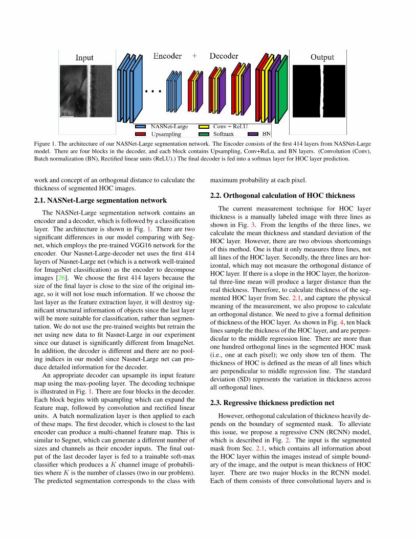
Figure 1. The architecture of our NASNet-Large segmentation network. The Encoder consists of the first 414 layers from NASNet-Largemodel. There are four blocks in the decoder, and each block contains Upsampling, Conv+ReLu, and BN layers. (Convolution (Conv),Batch normalization (BN), Rectified linear units (ReLU).) The final decoder is fed into a softmax layer for HOC layer prediction.

work and concept of an orthogonal distance to calculate thethickness of segmented HOC images.

2.1. NASNet-Large segmentation network

The NASNet-Large segmentation network contains anencoder and a decoder, which is followed by a classificationlayer. The architecture is shown in Fig. 1. There are twosignificant differences in our model comparing with Seg-net, which employs the pre-trained VGG16 network for theencoder. Our Nasnet-Large-decoder net uses the first 414layers of Nasnet-Large net (which is a network well-trainedfor ImageNet classification) as the encoder to decomposeimages [26]. We choose the first 414 layers because thesize of the final layer is close to the size of the original im-age, so it will not lose much information. If we choose thelast layer as the feature extraction layer, it will destroy sig-nificant structural information of objects since the last layerwill be more suitable for classification, rather than segmen-tation. We do not use the pre-trained weights but retrain thenet using new data to fit Nasnet-Large in our experimentsince our dataset is significantly different from ImageNet.In addition, the decoder is different and there are no pool-ing indices in our model since Nasnet-Large net can pro-duce detailed information for the decoder.

An appropriate decoder can upsample its input featuremap using the max-pooling layer. The decoding techniqueis illustrated in Fig. 1. There are four blocks in the decoder.Each block begins with upsampling which can expand thefeature map, followed by convolution and rectified linearunits. A batch normalization layer is then applied to eachof these maps. The first decoder, which is closest to the lastencoder can produce a multi-channel feature map. This issimilar to Segnet, which can generate a different number ofsizes and channels as their encoder inputs. The final out-put of the last decoder layer is fed to a trainable soft-maxclassifier which produces a K channel image of probabili-ties where K is the number of classes (two in our problem).The predicted segmentation corresponds to the class with

maximum probability at each pixel.

2.2. Orthogonal calculation of HOC thickness

The current measurement technique for HOC layerthickness is a manually labeled image with three lines asshown in Fig. 3. From the lengths of the three lines, wecalculate the mean thickness and standard deviation of theHOC layer. However, there are two obvious shortcomingsof this method. One is that it only measures three lines, notall lines of the HOC layer. Secondly, the three lines are hor-izontal, which may not measure the orthogonal distance ofHOC layer. If there is a slope in the HOC layer, the horizon-tal three-line mean will produce a larger distance than thereal thickness. Therefore, to calculate thickness of the seg-mented HOC layer from Sec. 2.1, and capture the physicalmeaning of the measurement, we also propose to calculatean orthogonal distance. We need to give a formal definitionof thickness of the HOC layer. As shown in Fig. 4, ten blacklines sample the thickness of the HOC layer, and are perpen-dicular to the middle regression line. There are more thanone hundred orthogonal lines in the segmented HOC mask(i.e., one at each pixel); we only show ten of them. Thethickness of HOC is defined as the mean of all lines whichare perpendicular to middle regression line. The standarddeviation (SD) represents the variation in thickness acrossall orthogonal lines.

2.3. Regressive thickness prediction net

However, orthogonal calculation of thickness heavily de-pends on the boundary of segmented mask. To alleviatethis issue, we propose a regressive CNN (RCNN) model,which is described in Fig. 2. The input is the segmentedmask from Sec. 2.1, which contains all information aboutthe HOC layer within the images instead of simple bound-ary of the image, and the output is mean thickness of HOClayer. There are two major blocks in the RCNN model.Each of them consists of three convolutional layers and is

Figure 2. The architecture of the thickness regression network. The input is from the NASNet-Large segmentation network. The thicknessregression network primarily consists of two blocks, and each block includes Conv + ReLU and Dropout layers. It is then followed by aFlatten layer. Finally, it ends with a linear activation layer. The output is the thickness of the HOC layer.

Figure 3. The existing three-line thickness measurement of theHOC layer. However, the three-line approach is manually labeled,and consists of horizontal lines, which will overestimate the thick-ness if within a slope or curve.

followed by one dropout layer. After that a flatten layer ex-pands all features in its front dropout layer into a vector.Two dense and activation layers follow. The regression net-work ends with a linear activation to predict the thicknessof the HOC layer. During the training stage of the RCNNmodel, the labeled thickness is from the proposed orthogo-nal calculation method.

There are two advantages of our RCNN model. First, theRCNN model is not complex and easy to train. If the archi-tecture is too complex, it may lead to an overfitting problem.One reason is the input is the segmented HOC layer, whichdoes not contain too much information. Hence, a complexneural network is unnecessary. Another advantage of the

Figure 4. The orthogonal distance of the HOC layer. Two reddashed lines are the boundaries of the HOC layer; the middle redline consists of midpoints of boundary points, and the blue dashedline is the regression line. Several black lines are the orthogonaldistance of the HOC layer. Lower right shows magnified greenbox.

RCNN model is that it can give a prediction with less error.In the training stage, the RCNN model is fed with the seg-mented mask and outputs orthogonal calculation distance.The loss function is mean squared error (MSE), which isdefined in Eq. 1.

MSE =1

n

n∑i=1

(Yi − Yi)2, (1)

where Yi is the prediction value, and Yi is the orthogonaldistance measurement as shown in Sec. 2.2. Therefore, weminimize the error between orthogonal distance using the

Figure 5. Four TEM HOC images and their corresponding HOCsegmentations.

predicted HOC mask and the orthogonal thickness. Thisfurther drives the prediction mean thickness to be close tothe orthogonal thickness.

Unfortunately, a deep network is often difficult to trustgiven its opacity. Domain experts prefer a clear measure-ment. However, the proposed RCNN model can be vali-dated, if needed, by the orthogonal calculation.

3. Results

3.1. Datasets

Our modeling was trained with data, that are collectedfrom three different dates, differing in the composition ofthe HOC material. Due to a limited sample size of 364 im-ages, we use five-fold cross-validation to estimate the per-formance of our model. We normalize pixel values of theimage into a scale between 0 and 1. Since we do not haveground truth for the mask of HOC layer, the TEM imagewas first marked by an expert using thickness measurementsoftware (an internally developed package based on Zhanget al. [23]) to manually segment the mask and output roughthickness. Fig. 5 shows four TEM images with their cor-responding segmentation labels. The middle two examplesin Fig. 5 cause difficulty with the HOC layer segmentation;there is a FOV (field of view) sticker in the third image,and there is an extra horizontal layer in the fourth image.Due to these reasons, the traditional threshold-based meth-ods failed in segmenting these three images.

Our experiments are implemented within Keras, and ournetwork was trained on an NVIDIA TITAN XP equippedwith 12 GB of memory in order to exploit its computationalspeed. The network parameters were set to: Batch size: 4,Step size: 5, Number of epochs: 1000.

3.2. Segmentation results visualization

Fig. 6 compares the predicted segmented HOC imagewith the ground truth image in the test dataset. The pre-diction image is close to the real mask, which qualitativelydemonstrates the high performance of our model.

Figure 6. Ground truth vs. prediction results. The first row is theground truth mask overlay with the raw image, and the second rowis the prediction result overlaid with the raw image.

Figure 7. The post-processing of prediction result. On the left isthe prediction result from the proposed network, and on the rightis the result after using our post-processing layer. The red boxoutlines an irrelevant feature.

3.3. Post-processing layer

However, there are some areas in the image which arenot the true HOC layer in the prediction result. We thenpropose a post-processing layer, which can filter the irrele-vant parts of the prediction. The first step of post-processinglayer is to classify the predicted image into several parts1,and we then simply select the largest areas (the HOC area)as the final segmented HOC layer. As shown in the left im-age in Fig. 7, the red box highlights erroneous predictionsof the image (false negatives). After post-processing, thered box is removed. Therefore, the prediction result can beimproved if we filter out such irrelevant parts.

3.4. Metrics

To evaluate the performance of our NASNet-Large seg-mentation network, we use the widely-used Dice coefficientindex to indicate the goodness of the segmentation results.Furthermore, we also report the IoU score. The two metrics

1The major step of post-processing step is using the connectedCompo-nentsWithStats function in OpenCV.

Figure 8. Sample output image. Left: the predicted result of ourmodel; right: the original image. The segmented mask is per-fectly overlapped with the original image (MT: mean thickness,SD: standard deviation).

are defined in the following formulas:

Dice = 2× |A ∩B||A|+ |B|

, IoU =|A ∩B||A ∪B|

,

where A is ground truth mask, and B is the prediction mask.We also compare our results with performance of state-of-the-art methods.

Table 1. Five-fold cross-validation segmentation resultsMethod IoU Dice scoreU-Net 0.80 0.85

Deep-Lab 0.83 0.89Segnet 0.78 0.83

NastnetLarge-net 0.86 0.92NastnetLarge-net-post 0.89 0.94

Tab. 1 lists the comparison results of different mod-els (the metrics are only reported on HOC layer and notthe background area). Our NASNet-Large-Decoder has ahigher IoU and Dice score than other models. We alsoobserve that the method including post-processing outputsthe highest scores, which illustrates that the post-processinglayer is useful in our segmentation task.

We use MSE to evaluate the performance of RCNNmodel and traditional orthogonal distance calculation as de-fined in Eq. 1. As shown in Tab. 2, the MSE of RCNNmodel is less than the other three methods, which impliesthat RCNN model gives a closer prediction to orthogo-nal measurement than Segnet RCNN and NASNet-LargeRCNN. Differing from original Segnet and NASNet-Largemodel, we replace the final softmax layer with a regressivelayer to form the Segnet RCNN and NASNet-Large RCNNmodel. Hence, these two models are able to predict thethickness. Fig. 8 shows the final output of our thicknessmeasurement tool. The left image is the segmented HOClayer overlay with original image, and it also shows orthog-onal distance. We also add the file name, mean thickness

(a) Training with 0.0929 MSE

(b) Test with 0.0719 MSE

Figure 9. Comparison of the existing three-line method and ourpredication in training and test datasets.

and standard deviation of the thickness on the top of theimage.

Table 2. Thickness prediction results comparisonMethods MSE

Regressive CNN 0.0089Three-line measurement 0.1524

Segnet RCNN 0.1792NASNet-Large RCNN 0.2023

4. DiscussionIn this section, we first analyze predicted HOC thickness

and then discuss the merits and demerits of our model.

4.1. Statistical analysis

As shown in Fig. 9, we compare the three-line measure-ments with orthogonal distance from predicted HOC mask

(a) (2.40, 1.58) (b) (4.29, 3.63)

Figure 10. Two outlier images, which correspond to the high-lighted points in Fig. 9(a). Labels are (X,Y) pairs. X-value isthe thickness from three-line measurement and y-value is the pre-diction value from orthogonal distance.

Figure 11. Linear regression fit of predicted thickness and the three-line thickness (Different color represents data are collected fromdifferent dates).

using linear regression in training and test datasets, respec-tively. The blue dashed lines in the figure indicate the de-sired line if prediction results are the same as the humanthree-line measurements. The regression slope from train-ing and test are 0.79968 and 0.99155, respectively, whichdemonstrate a strong linear correlation between the humanmeasurement and deep learning method. Especially noti-cable is the test dataset, in which the prediction is almostthe same as human measurement. We also calculate themean squared error (MSE) in Eq. 1 to indicate the error be-tween deep learning prediction and human measurement.Although there are some outliers in Fig. 9(a), eg., (2.40,1.58) and (4.29, 3.63) (the x-value is three-line result and y-value is prediction results from our model), the overall per-formance of the orthogonal measurement method is closerto human measurement. The three-line method has a highervalue than deep learning prediction in these two off-linepoints. We further check the prediction mask images ofthese two points as shown in Fig. 10. We observe that there

(a) Deep learning prediction

(b) Human measurement

Figure 12. TEM human 3-line measurement and TEM deep learn-ing prediction compared against measurements made with witnesswafer metrology. Deep learning prediction gives more accurateresults than human three-line measurement.

is a slope in these two prediction HOC layer. Remember,the three-line is measured using horizontal lines, which willlead to a higher value than the real distance if there is a slopein the boundary of mask images. However, we calculateorthogonal distance, which represents the real thickness ofthe HOC layer. Therefore, we can conclude that our methodcan be applied in thickness measurements, and it will leadto better results than human three-line measurement.

Fig. 11 describes overall performance in the training andtest in terms of three different data collection dates us-ing the mean thickness and standard deviation. We fur-ther compare the prediction thickness from our model andthe three-line approach with measurements made on wit-ness wafers included in the same HOC depositions as theproduct heads that were measured with TEM. The witnesswafers were measured using metrology calibrated using an

Figure 13. Two failures in NASNet-Large-Decoder model. Thefirst row of image is caused by the fuzzy boundary and the secondrow of image is caused by the unusually dark HOC layer.

amalgamation of techniques, such as AFM (Atomic ForceMicroscopy), ellipsometry, and XRR (X-Ray Reflectome-try).

From Fig. 12, we can find that the deep learning-basedmodel has slightly worse results in sample set #1 since theslope is smaller than the three-line measurement (0.98546vs. 0.99119 ). However, the performance in sample set#2 is significantly higher than the three-line measurement(0.90861 vs. 0.8068). Also, the overall prediction of ourmodel is better than human measurement (as shown in thegreen lines in Fig. 12 ). Therefore, we can conclude thatour model has a better performance than traditional manualmeasurement.

Although the RCNN model gives more accurate resultsthan three-line measurement (as shown in Tab. 2), we didnot use it to predict thickness of test datasets. The crucialreason is that customers require a comparison image forthickness measure as shown in Fig. 8. But RCNN modelcannot output images with actual calculation of distance(i.e., cannot output an image as in the left of Fig. 8). Henceit is not used on test datasets. However, RCNN model is aback-up model if the orthogonal distance failed.

One of the distinct advantages of our model is that itachieves a higher Dice and IoU score. And there aretwo reasons: the designed NASNet-Large segmentation netis suitable for TEM image segmentation, and the post-processing layer filters out the unnecessary parts in the im-age, which improves the segmented results.

Although our model achieves a 0.94 Dice score, it stillfails in some cases. As shown in Fig. 13, we observethat segmentation results are worse in these two situations.There are two reasons; one is that there is no similar imagein the training dataset, which leads to worse performance.Second is that our model is not robust enough to deal withsome unusual images. Comparing with normal training im-

ages as shown in Fig. 5, two worse raw images (in Fig. 13)are either too light (first row) or too dark (second row), andit is even difficult for humans to distinguish the HOC layerand background. Also, our model has limited sample size(less than 400 images), and so while in the validation andtest datasets the MSE is small, our model could not coverall the cases, e.g., in Fig. 13. Therefore, including moresamples in training would help to get a more robust model.In addition, a limitation of the NASNet-Large-Decoder net-work is that it needs a large memory to train the model.Therefore, designing a more efficient architecture is a di-rection for future work.

5. Conclusion

In this paper, we are the first to present a TEM HOClayer segmentation using the NASNet-Large-decoder archi-tecture, and we get an accurate segmentation with 0.94 Dicescore. A post-processing layer is employed to remove theunnecessary part in the prediction map. We then propose anorthogonal thickness calculation method as well as a regres-sive convolutional neural network (RCNN) model to mea-sure the thickness of the segmented HOC layer. These ad-vances enable manufacturers to replace a manual methodwith a much more accurate automated process.

Our model can be further improved with a more robustencoder and decoder model, to enable it to be applied in awider variety of cases. The RCNN model can also be en-hanced by predicting both the mean thickness and the stan-dard deviation of the mean thickness.

References[1] M. Awad. An unsupervised artificial neural network method

for satellite image segmentation. Int. Arab J. Inf. Technol.,7(2):199–205, 2010. 1

[2] M. Awad, K. Chehdi, and A. Nasri. Multicomponent imagesegmentation using a genetic algorithm and artificial neu-ral network. IEEE Geoscience and remote sensing letters,4(4):571–575, 2007. 1

[3] V. Badrinarayanan, A. Kendall, and R. Cipolla. Segnet: Adeep convolutional encoder-decoder architecture for imagesegmentation. IEEE transactions on pattern analysis andmachine intelligence, 39(12):2481–2495, 2017. 2

[4] L.-C. Chen, G. Papandreou, I. Kokkinos, K. Murphy, andA. L. Yuille. Semantic image segmentation with deep con-volutional nets and fully connected crfs. arXiv preprintarXiv:1412.7062, 2014. 2

[5] J. Freixenet, X. Munoz, D. Raba, J. Martı, and X. Cufı. Yetanother survey on image segmentation: Region and bound-ary information integration. In European Conference onComputer Vision, pages 408–422. Springer, 2002. 1

[6] B. Fultz and J. M. Howe. Transmission electron microscopyand diffractometry of materials. Springer Science & Busi-ness Media, 2012. 1

[7] A. Garcia-Garcia, S. Orts-Escolano, S. Oprea, V. Villena-Martinez, and J. Garcia-Rodriguez. A review on deep learn-ing techniques applied to semantic segmentation. arXivpreprint arXiv:1704.06857, 2017. 2

[8] K. Hammouche, M. Diaf, and P. Siarry. A multilevel auto-matic thresholding method based on a genetic algorithm fora fast image segmentation. Computer Vision and Image Un-derstanding, 109(2):163–175, 2008. 1

[9] K. He, X. Zhang, S. Ren, and J. Sun. Spatial pyramid poolingin deep convolutional networks for visual recognition. IEEEtransactions on pattern analysis and machine intelligence,37(9):1904–1916, 2015. 2

[10] S. Hu, E. A. Hoffman, and J. M. Reinhardt. Automatic lungsegmentation for accurate quantitation of volumetric x-ray ctimages. IEEE transactions on medical imaging, 20(6):490–498, 2001. 2

[11] L. Kang, P. Ye, Y. Li, and D. Doermann. Convolutional neu-ral networks for no-reference image quality assessment. InProceedings of the IEEE conference on computer vision andpattern recognition, pages 1733–1740, 2014. 2

[12] C. Li, R. Huang, Z. Ding, J. C. Gatenby, D. N. Metaxas, andJ. C. Gore. A level set method for image segmentation inthe presence of intensity inhomogeneities with applicationto mri. IEEE transactions on image processing, 20(7):2007–2016, 2011. 1

[13] C. Li, C. Xu, C. Gui, and M. D. Fox. Distance regularizedlevel set evolution and its application to image segmentation.IEEE transactions on image processing, 19(12):3243–3254,2010. 1

[14] J. Long, E. Shelhamer, and T. Darrell. Fully convolutionalnetworks for semantic segmentation. In Proceedings of theIEEE conference on computer vision and pattern recogni-tion, pages 3431–3440, 2015. 2

[15] J. Ning, L. Zhang, D. Zhang, and C. Wu. Interactive imagesegmentation by maximal similarity based region merging.Pattern Recognition, 43(2):445–456, 2010. 1

[16] J. Pu, J. Roos, A. Y. Chin, S. Napel, G. D. Rubin, and D. S.Paik. Adaptive border marching algorithm: automatic lungsegmentation on chest ct images. Computerized MedicalImaging and Graphics, 32(6):452–462, 2008. 2

[17] W. E. Reddick, J. O. Glass, E. N. Cook, T. D. Elkin, and R. J.Deaton. Automated segmentation and classification of mul-tispectral magnetic resonance images of brain using artificialneural networks. IEEE Transactions on medical imaging,16(6):911–918, 1997. 1

[18] O. Ronneberger, P. Fischer, and T. Brox. U-net: Convo-lutional networks for biomedical image segmentation. InInternational Conference on Medical image computing andcomputer-assisted intervention, pages 234–241. Springer,2015. 2

[19] R. Rothe, R. Timofte, and L. Van Gool. Dex: Deep expec-tation of apparent age from a single image. In Proceedingsof the IEEE International Conference on Computer VisionWorkshops, pages 10–15, 2015. 2

[20] W.-B. Tao, J.-W. Tian, and J. Liu. Image segmentationby three-level thresholding based on maximum fuzzy en-tropy and genetic algorithm. Pattern Recognition Letters,24(16):3069–3078, 2003. 1

[21] O. J. Tobias and R. Seara. Image segmentation by histogramthresholding using fuzzy sets. IEEE transactions on ImageProcessing, 11(12):1457–1465, 2002. 1

[22] L. A. Vese and T. F. Chan. A multiphase level set frame-work for image segmentation using the mumford and shahmodel. International journal of computer vision, 50(3):271–293, 2002. 1, 2

[23] C. Zhang, K. Loken, Z. Chen, Z. Xiao, and G. Kunkel. Maskeditor: an image annotation tool for image segmentationtasks. arXiv preprint arXiv:1809.06461, 2018. 5

[24] J. Zhang and J. Hu. Image segmentation based on 2d otsumethod with histogram analysis. In 2008 International Con-ference on Computer Science and Software Engineering, vol-ume 6, pages 105–108. IEEE, 2008. 1

[25] Y. Zhang and Q. Li. A regressive convolution neural networkand support vector regression model for electricity consump-tion forecasting. In Future of Information and Communica-tion Conference, pages 33–45. Springer, 2019. 2

[26] B. Zoph, V. Vasudevan, J. Shlens, and Q. V. Le. Learningtransferable architectures for scalable image recognition. InProceedings of the IEEE conference on computer vision andpattern recognition, pages 8697–8710, 2018. 3