DEPARTMENT OF ECONOMICS

Automatic Grade Promotion and Student

Performance: Evidence from Brazil

Martin Foureaux Koppensteiner, University of Leicester, UK

Working Paper No. 11/52

November 2011

Automatic Grade Promotion and Student Performance:

Evidence from Brazil

Martin Foureaux Koppensteiner*

This version: November 2011

Abstract

This paper examines the effect of the introduction of automatic grade promotion on

student performance in 1,993 public primary schools in the Brazilian state of Minas

Gerais. A difference-in-difference approach that exploits variation over time in the

adoption of the policy allows the identification of the treatment effect of automatic

promotion. I find a negative and significant effect of about 6% of a standard deviation.

Under plausible identifying assumptions the estimates can be interpreted as the

disincentive effect on student effort associated with the introduction of automatic

promotion.

Keywords: Grade retention, automatic promotion, incentives for effort.

JEL numbers: I28, I21, O15, H52

_________________________________________________

I am very grateful to Marco Manacorda for invaluable advice and guidance. I also thank David Card,

Jefferson Mainardes, Imran Rasul and seminar participants at University College London, Queen Mary,

the International Conference on the Economics of Education in Zurich 2008, the Spring Meeting of

Young Economists 2010, and the Congress of the European Economic Association 2010 for valuable

comments. I am grateful to the Secretariat of Education in Minas Gerais, the Brazilian Ministry of

Education and the National Institute for Educational Studies and Research (INEP) for the data. I thank

Juliana Riani and Jorge Rondelli for assistance obtaining the data. The usual disclaimer applies.

* Department of Economics, University of Leicester, University Road, Leicester, LE1 7HR.

Email: mfkoppensteiner@le.ac.uk. Telephone: +44 116 252 2467.

1. INTRODUCTION

Grade retention,1 the practice of holding back students in the same grade for an extra year if

they fail to achieve promotion requirements, either in the form of a performance measure or

in the form of minimum attendance, is used in many developing and in some developed

countries. It is particularly widespread and pronounced in African and Latin American

countries, where repetition rates are often as high as 30% (UNESCO 2008).2 Historically

grade repetition had a prominent role in Brazil and repetition rates in Brazilian primary

schools reached 24% in 1st grade and 14% in 4

th grade in 2005.

3

Retaining students has important consequences both for the individual as well as for the

school system overall. Overall, every repeater has the same effect on school resources as

enrolling an additional student at that grade and subsequent grades and either leads to

compromising per pupil school inputs e.g. through larger class size or to a pressure on public

finances through the additional demand for teachers, classrooms, desks and other inputs.4

Opponents of grade repetition contend that it negatively impacts on the retained individual by

stigmatizing them and harming their self-esteem, by impairing established peer relationships

and generally alienating the individual from school, which may in turn negatively impact on

academic achievement and increase probability of dropping-out of school (Holmes 1989).

Furthermore, repeating grades delays entrance of students into the labour market which poses

substantial monetary cost on students over the life-cycle. In contrast, proponents argue that

repetition can improve academic achievement by exposing low performing students to

additional teaching and allowing them to catch up on the curriculum and the content of

teaching. This is particularly important if school absence for reasons such as illness in a

specific school year is the reason for retention. Grade retention may also help to make classes

more homogeneous in achievement and therefore easier to teach by improving the match

between peers in the classroom.

Studies that try to tackle the selection problem and deal with the potential endogeneity of

grade failure leave a rather inconclusive picture of the direction of the effect. Eide and

Showalter (2001) present evidence from the „High School and Beyond‟ survey on US high-

1 In the literature also referred to as grade repetition.

2 40 out of 43 African countries for which data is available in 2006 use grade retention (and for which average

repetition rates exceed 4% in primary school) and 18 out of 23 Latin American and Caribbean countries. 3 Data available at http://stats.uis.unesco.org/unesco/ReportFolders/ReportFolders.aspx. UNESCO Institute for

Statistics, Data Centre, January 2008. 4 A very rough estimate of the annual cost of repetition on public finances in Brazil using average expenditure

per pupil at primary schools in 2006 of $554 (in constant 2005 US$) and 18,661,000 students enrolled at

primary school and an average repetition rate over all grades of 18.7% (not accounting for loss of students due

to drop-out etc.) amounts to approximately 1.9 billion US$ (all data from UNESCO 2008).

3

school students to assess the impact of grade retention on the probability of dropping out of

high-school. They report a reduction of drop-out rates and increased labour market earnings

for white students, but their IV estimates are not statistically significant at conventional

levels. Dong (2009) uses a control-function approach and reports positive effects of retention

on academic performance of a representative sample of kindergarten children in the U.S.

Jacob and Lefgren (2004) use a regression-discontinuity design exploiting the discontinuous

relationship between test scores and promotion to estimate the causal effect of repetition for

3rd

and 6th

grade public school students in Chicago. They find that repetition increases

achievement for third-graders in the short-run, but find no effect on 6th

graders math

achievement (and a negative effect for reading). Using a similar identification strategy Jacob

and Lefgren (2009) examine the long-run effects of repetition on high school completion

focussing again on Chicago public school students. They find that repetition has no effect on

the likelihood for high school completion of 3rd grade students, but negatively affects the

probability of 8th

grade students to complete high school.

Manacorda (2011) provides quasi-experimental evidence for a middle-income country

analysing the effect of retention on student drop-out at junior high school in Uruguay.5 He

uses the discontinuity of the promotion rule induced by minimum attendance requirements to

investigate the long-run consequences of grade failure. His findings point to long-lasting

negative effects on educational attainment and an increase in drop-out rates as a result of

grade retention.

Using variation across schools in test score variation Glick and Sahn (2010) show that

repeaters are more likely to leave school before completing primary school in Senegal.

Considering the mixed empirical results on the effect on repeaters, the use of public resources

and the undesirable consequences for public finances, the persistence of grade retention

regimes in many countries is puzzling. This is particularly the case for developing countries

where repetition rates are often very high and pressure on public resources is even higher.

Even when assuming positive effects on achievement of repeaters, this leaves an equity

question to the policy maker, as the cost associated with wide-spread retention may be levied

on all students in terms of an increase in class-size and a reduction of per-pupil resources, but

benefits are limited to repeaters.6 Furthermore, repetition increases the age variation in the

5 The only available attempts to assess grade retention on student outcomes for Brazil are by Gomes-Neto &

Hanushek (1994) and Ferrão, Beltrão & dos Santos (2002). They nevertheless do not account for endogeneity of

grade failure. 6 Leaving potential positive spillover effects from “treated” repeaters on the peer in the classroom unconsidered.

4

classroom and repeaters may also directly lead to negative externalities on their peer students

(Lavy, Paserman and Schlosser 2011).

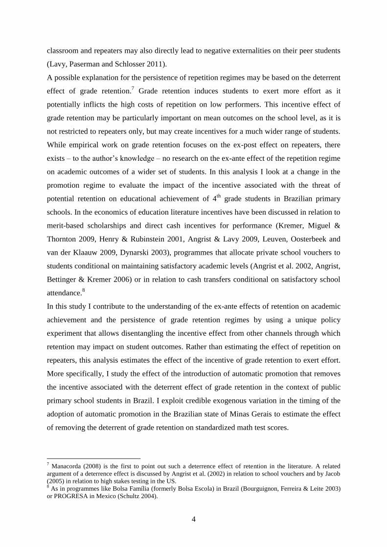
A possible explanation for the persistence of repetition regimes may be based on the deterrent

effect of grade retention.7 Grade retention induces students to exert more effort as it

potentially inflicts the high costs of repetition on low performers. This incentive effect of

grade retention may be particularly important on mean outcomes on the school level, as it is

not restricted to repeaters only, but may create incentives for a much wider range of students.

While empirical work on grade retention focuses on the ex-post effect on repeaters, there

exists – to the author‟s knowledge – no research on the ex-ante effect of the repetition regime

on academic outcomes of a wider set of students. In this analysis I look at a change in the

promotion regime to evaluate the impact of the incentive associated with the threat of

potential retention on educational achievement of 4th

grade students in Brazilian primary

schools. In the economics of education literature incentives have been discussed in relation to

merit-based scholarships and direct cash incentives for performance (Kremer, Miguel &

Thornton 2009, Henry & Rubinstein 2001, Angrist & Lavy 2009, Leuven, Oosterbeek and

van der Klaauw 2009, Dynarski 2003), programmes that allocate private school vouchers to

students conditional on maintaining satisfactory academic levels (Angrist et al. 2002, Angrist,

Bettinger & Kremer 2006) or in relation to cash transfers conditional on satisfactory school

attendance.8

In this study I contribute to the understanding of the ex-ante effects of retention on academic

achievement and the persistence of grade retention regimes by using a unique policy

experiment that allows disentangling the incentive effect from other channels through which

retention may impact on student outcomes. Rather than estimating the effect of repetition on

repeaters, this analysis estimates the effect of the incentive of grade retention to exert effort.

More specifically, I study the effect of the introduction of automatic promotion that removes

the incentive associated with the deterrent effect of grade retention in the context of public

primary school students in Brazil. I exploit credible exogenous variation in the timing of the

adoption of automatic promotion in the Brazilian state of Minas Gerais to estimate the effect

of removing the deterrent of grade retention on standardized math test scores.

7 Manacorda (2008) is the first to point out such a deterrence effect of retention in the literature. A related

argument of a deterrence effect is discussed by Angrist et al. (2002) in relation to school vouchers and by Jacob

(2005) in relation to high stakes testing in the US. 8 As in programmes like Bolsa Família (formerly Bolsa Escola) in Brazil (Bourguignon, Ferreira & Leite 2003)

or PROGRESA in Mexico (Schultz 2004).

5

I find that the introduction of automatic promotion significantly reduces academic

achievement measured by math test scores of 4th

graders by 6% of a standard deviation.

Under plausible assumptions I argue for the interpretation of the results as the disincentive

effect of the introduction of automatic promotion.

The remainder of the paper is organized as follows. Section 2 provides information on the

school system in Brazil and in the state of Minas Gerais. Section 3 presents the data. Section

4 describes the natural experiment and outlines the assignment of schools to treatment.

Section 5 introduces the empirical strategy. The results, their interpretation and falsification

exercises are presented in section 6, and section 7 concludes.

2. THE SCHOOL SYSTEM IN BRAZIL AND MINAS GERAIS

Primary school is compulsory in Brazil for children between the ages of 7 to 14 and consists

of eight years of schooling (MEC 1996).9 Public schooling is free at all ages and enrolment in

primary and secondary school is open to students of all ages.

The Brazilian educational system has undergone substantial changes during the last two

decades and has achieved considerable progress in expanding access to education. Starting

from a primary school net enrolment rate of only 85% in 1991, Brazil achieves today almost

universal primary school enrolment with a net rate of 95% (UNESCO 2009). Primary school

completion and youth literacy rates have improved notably, but the country continues to

suffer from high repetition and drop-out rates.10

The national conditional cash transfer programme Bolsa Família, formerly Bolsa Escola,

which is a means-tested monthly cash transfer to poor households conditional on school

enrolment and regular attendance among other conditions, plays a significant role for the rise

in school enrolment and attendance of school age children (de Janvry, Finan & Sadoulet

2006).11

This analysis focuses on the state of Minas Gerais, the second most populous state in Brazil

with an estimated population of about 19 million (IBGE 2007). Minas Gerais contributes

10% to the Brazilian GDP and is among the most developed states in Brazil (OECD 2005).

9 The school entry age has been lowered recently to 6 years and primary school has been extended to 9 years.

10 The overall repetition rate in primary schools in Brazil in 2006 was 18.7% and the total drop-out rate for

primary school 19.5% (UNESCO 2009). 11

The conditionalities of Bolsa Família require a minimum school attendance of 85% and extend to the

fulfilment of basic health care requirements such as vaccinations of the children and pre and postnatal medical

consultations for pregnant women. Monthly per capita income in the household cannot exceed R$120 (US$57 in

2006) to remain eligible for the transfer. See Lindert et al. 2007 for a comprehensive description of the

programme.

6

The education system of Minas Gerais is among the most developed and in national

performance tests students continue to be among the top 5 states (INEP 2007).

According to state legislation, the State Secretariat of Education (SEE) has extensive

authority to plan, direct, execute, control and evaluate all educational activities in Minas

Gerais. Based on far-reaching decentralization of education in Brazil, the SEE transfers

authority to a large extent to Regional Authorities for Education (Superintendências

Regionais de Ensino: SREs) and directly to the municipalities. SREs and municipalities

therefore play a major role in the provision of schooling and the implementation of

educational policies.12

Municipal schools account for more than half (56%) of all primary

schools and state schools, that are directly under the control of the SEE, account for 22% of

all schools. Outside the public education system private schools play an important role and

account for the remaining 22%.13

3. DATA DESCRIPTION

This study uses data from two sources. Information on school characteristics comes from the

annual Brazilian school census that is conducted by the National Institute for the Study and

Research on Education (INEP) under the control of the Federal Ministry of Education

(MEC). The Brazilian school census compiles data annually from all primary and secondary

schools in Brazil. The exceptionally rich data includes information on the location and

administrative dependence of schools, physical characteristics (quantity of premises and class

rooms, equipment and teaching material), the participation in national, state and municipal

school programmes, the number of teachers and administrative staff, average class-size,

detailed information on student flows (number of students in each grade according to age,

repetition, drop-out and student transfer rates) among other information. Summary statistics

for the public schools used in this analysis are presented in panel A of table A1 in the annex.

The school census also contains the information on the regime of grade promotion adopted in

each school (grade retention versus automatic promotion), which is used to establish

treatment and control groups.

The second part of the data comes from the State System of the Evaluation of Public

Education (Sistema Mineiro de Avaliação da Educação Pública: SIMAVE), which includes

12

The installation of FUNDEF, a federal fund established in 1996 with the aim of redistributing state and

municipal resources back to (mainly) municipalities according to student numbers contributed to the

improvement of the control of municipalities over educational decisions. See de Mello & Hoppe (2005) for an

analysis of FUNDEF. 13

There are also 28 federal schools in Brazil which are under the direct control of the federal government; the

single federal school in Minas Gerais has not been included in the dataset.

7

the programme for the evaluation of primary and secondary schools (Programa de Avaliação

da Educação Básica: PROEB).

The main outcome variable is student achievement in state schools in Minas Gerais measured

by math test scores in 2003 and 2006. All classes and all students in 4th

grade of each school

are examined and participation of schools and pupils is compulsory. The cognitive test scores

are standardized to a mean of 500 and a standard deviation of 100. In total 246,959 students

have been tested in 1,993 state schools in Minas Gerais. I use the repeated cross-section of

test score data from 2003 and 2006 for this analysis. The students in the dataset have, as

generally students in public schools, a deprived socioeconomic background. Almost half

(45.6%) of the families with children at state schools in Minas Gerais qualify for Bolsa

Família and can be considered poor. Information on sex, date of birth, racial background and

on the socio-economic family background also is available from an adjunct questionnaire.

Chart B of table A1 presents summary statistics on these variables.

4. THE GENERAL EDUCATION ACT OF 1996: THE CASE OF A QUASI-

EXPERIMENT

4.1 Policy background

The General Education Act of 1996 (Lei de Diretrizes e Bases da Educação Nacional: LDB)

paved the way for the introduction of automatic promotion policies in Brazil. Federal Law No

9.394/1996, which came into effect in 1998, regulates the responsibility for education

between the federal, state and municipal level and facilitated federal and state programmes to

control the grade promotion regime (Pino & Koslinski 1999). Section 3 of Art. 32 §1&2

formally distinguishes two alternatives for educational authorities to organize student

progression: besides the conventional annual grade repetition regime the option of automatic

promotion was introduced, a system in which students progress automatically to the next

grade at the end of the school year. Between these two extremes, a mixture of both regimes

was also permitted. In the mixed regime, schools define “learning cycles” that stretch over

several – most commonly three - school years. During the initial years of the cycle students

are promoted automatically. In the final year of a cycle students that do not meet the

minimum requirements set in the curriculum are retained. The idea behind these learning

cycles is to allow students an individual studying pace (Mainardes 2004). If students fall

behind their classmates they have a longer period to catch up on the curriculum. This

particularly aims at reducing the long-run impact of negative temporary shocks, such as

school days lost to sickness or adverse family events. With the mixed regime schools that

8

have adopted automatic promotion in learning cycles, grade retention is not entirely

eliminated, but limited to the final years of the cycles. The LDB furthermore sets

fundamental criteria on how to organize promotion under any one regime: In every school

year a minimum attendance of 75% of all school days must be fulfilled as a general

requirement for promotion, so that grade retention is still permitted in exceptional cases

where students fail to achieve 75% minimum attendance rule.

According to the legal framework of the LDB the decision on the promotion regime and its

exact specifications is taken on the state level. Automatic promotion was introduced at an

early stage by the states of São Paulo, Minas Gerais and Paraná, and to some extent in the

state of Pernambuco and by the federal resolution SE No 4, 1/98 in all federal schools in

Brazil. Only very recently a federal resolution has been passed to disallow retention for the

first three schools years in all schools in Brazil to take effect from 2011.

In the state of Minas Gerais the new regime has been established by state resolution No.

8.086 in 1997. It stresses the autonomy of each public school in the decision whether to

continue with the annual repetition regime or to introduce automatic promotion. I use the

variation in the repetition regime this freedom in the choice of the regime creates over time

and across schools for identification of the effect of the policy change. In the year 2000 1,449

out of 1,993 state schools had established automatic promotion with two initial three-year

cycles. At the beginning of the school year 2004 the remaining 544 state schools switched to

automatic promotion.

4.2 Assignment to treatment

I take schools that adopted automatic promotion at the beginning of the year 2004 as the

treatment group and schools with automatic promotion (which have adopted automatic

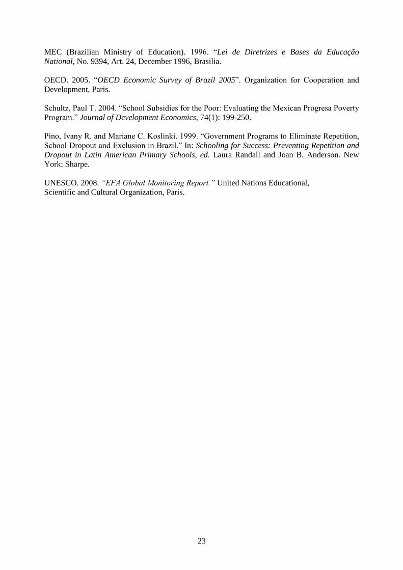
promotion since the year 2000) as the control group. I focus on two cohorts of 4th

graders,

which I call the test cohorts 2003 and 2006 for which test scores are available. Chart 1

presents an overview of these two cohorts and the change in the organization of promotion

for the control and treatment group.

When using this division into treatment and control group for comparison a sound

understanding of the assignment process that leads to this division is essential. In the case of

state schools in Minas Gerais the 46 regional authorities for education were asked to propose

a plan of implementation of automatic promotion for the schools under their administration.

The decision for early adoption of the policy was made by each SRE in agreement with the

state secretariat. The second wave was initiated by the SEE in an attempt to make automatic

9

promotion universal for all schools. As the adoption of the policy is not randomized across

schools in an experimental setting, treatment and control schools may not be balanced in the

distribution of school and mean pupil characteristics. Although the identification strategy

employed in this analysis does not rely on the distribution of covariates being balanced, it is

generally reassuring to find school and mean pupil characteristics of treatment and control

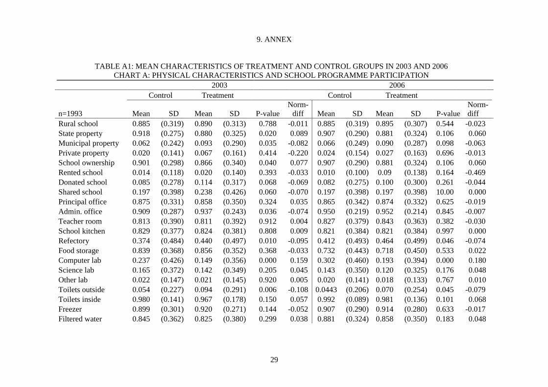
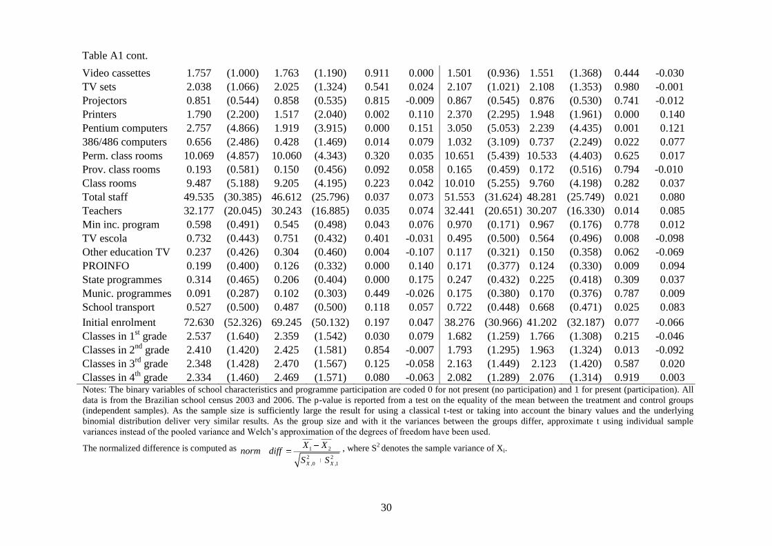
group to be very similar. Table A1, chart A and B present descriptive characteristics of

treatment and comparison schools for 2003 and 2006. T-tests (and Chi-square for categorical

variable) for the equality of means between treatment and comparison group, accounting for

clustering on the SRE level, reveal only very few small but statistically significant

differences. As sample size is partly reflected in the t-statistics, it is more useful to look at the

normalized difference 1 2

2 2

,0 ,1X X

X Xnorm diff

S S between means by treatment status as a

scale-free measure of the balancing properties of the covariates (Imbens & Wooldridge

2009). The normalized difference is small for all covariates and never exceeds the absolute

value 0.25,14

suggesting that treatment and control schools are in fact extremely similar in

terms of their physical school characteristics. Even more importantly, the normalized

differences for mean student characteristics, which may indicate compositional differences of

the student populations, are all very small and are far below the suggested rule-of-thumb

value of |0.25| in both years. Apart from mean age, which differs slightly as expected,15

no

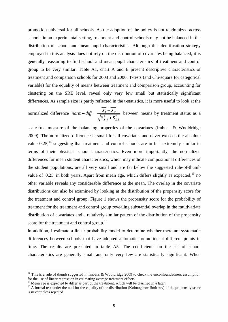
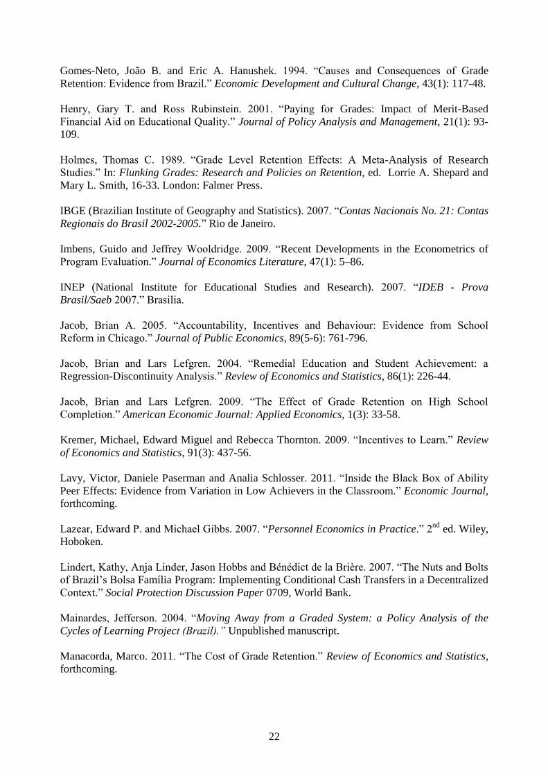
other variable reveals any considerable difference at the mean. The overlap in the covariate

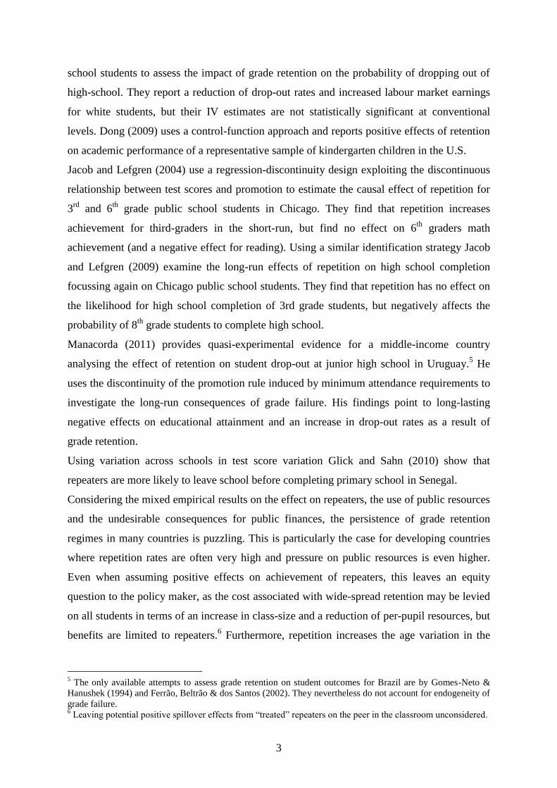
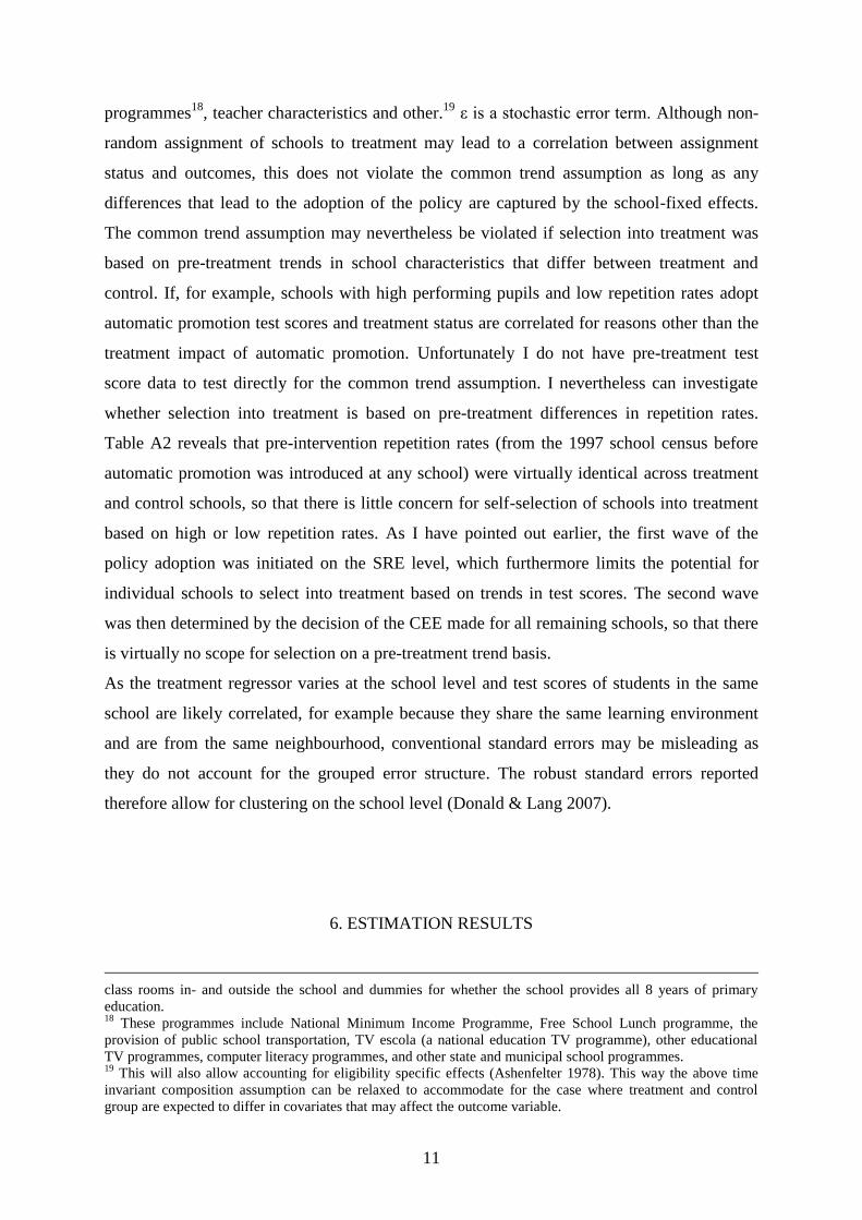
distributions can also be examined by looking at the distribution of the propensity score for

the treatment and control group. Figure 1 shows the propensity score for the probability of

treatment for the treatment and control group revealing substantial overlap in the multivariate

distribution of covariates and a relatively similar pattern of the distribution of the propensity

score for the treatment and control group.16

In addition, I estimate a linear probability model to determine whether there are systematic

differences between schools that have adopted automatic promotion at different points in

time. The results are presented in table A5. The coefficients on the set of school

characteristics are generally small and only very few are statistically significant. When

14

This is a rule of thumb suggested in Imbens & Wooldridge 2009 to check the unconfoundedness assumption

for the use of linear regression in estimating average treatment effects. 15

Mean age is expected to differ as part of the treatment, which will be clarified in a later. 16

A formal test under the null for the equality of the distribution (Kolmogorov-Smirnov) of the propensity score

is nevertheless rejected.

10

including SRE controls even fewer variables show a significant effect and it is difficult to

establish any systematic pattern.

Given the similarity of treatment and control schools with respect to the distribution of school

characteristics and the student composition, it is plausible to consider the assignment of

schools to treatment and control groups as conditionally random.

5. EMPIRICAL STRATEGY

To estimate the treatment effect of the policy change I use a difference-in-difference (DiD)

estimator exploiting the variation in treatment status of schools over time, identifying an

average treatment effect on individuals at schools assigned to treatment. The double

difference approach is capable of removing biases resulting from permanent latent

differences between treatment and control as well as biases resulting from common trends

over time. The estimation in a regression setup allows including additional regressors on the

individual and school level to improve precision and to test for the presence of omitted-

school specific trends, in particular related to potential changes in the student composition.

Identification requires that trends in student outcomes at treated and control schools would

not be systematically different in the absence of treatment.

Under this identifying assumption, I estimate the effect of the introduction of automatic

promotion on test scores of 4th

graders by the following regression model:

0 1 2ist s t st it st istY d d d Z X (1)

where Yist is the test score for individual i in school s at time t, ds is a school dummy which

captures school-specific time invariant effects, dt is a time dummy which captures the

common time trend of control and treatment group, dst is the time/treatment-status interaction

term containing information on treatment status of the schools, that varies over time. γ in

equation (1) is the coefficient of interest and reflects the average treatment effect of the

introduction of automatic promotion on test scores of 4th

graders. Zit is a set of covariates

controlling for individual characteristics. Xst denotes a set of exogenous covariates for class

and school characteristics, including average socioeconomic characteristics of students,

detailed school characteristics,17

the participation in federal, state and municipal educational

17

Specifically, the covariates include initial (1st grade) enrolment, number of teachers at school, number of total

staff (besides teaching staff), dummy variables describing the type of the premises used for the school, dummies

for the availability and number of teaching material (e.g. overhead projectors, personal computers, TV and video

sets etc.), the availability of computer and science labs, school kitchen, the quality of sanitary units, number of

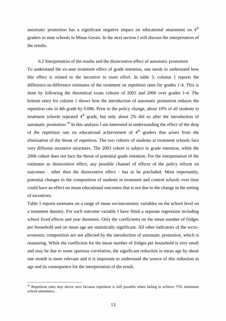
11

programmes18

, teacher characteristics and other.19

ε is a stochastic error term. Although non-

random assignment of schools to treatment may lead to a correlation between assignment

status and outcomes, this does not violate the common trend assumption as long as any

differences that lead to the adoption of the policy are captured by the school-fixed effects.

The common trend assumption may nevertheless be violated if selection into treatment was

based on pre-treatment trends in school characteristics that differ between treatment and

control. If, for example, schools with high performing pupils and low repetition rates adopt

automatic promotion test scores and treatment status are correlated for reasons other than the

treatment impact of automatic promotion. Unfortunately I do not have pre-treatment test

score data to test directly for the common trend assumption. I nevertheless can investigate

whether selection into treatment is based on pre-treatment differences in repetition rates.

Table A2 reveals that pre-intervention repetition rates (from the 1997 school census before

automatic promotion was introduced at any school) were virtually identical across treatment

and control schools, so that there is little concern for self-selection of schools into treatment

based on high or low repetition rates. As I have pointed out earlier, the first wave of the

policy adoption was initiated on the SRE level, which furthermore limits the potential for

individual schools to select into treatment based on trends in test scores. The second wave

was then determined by the decision of the CEE made for all remaining schools, so that there

is virtually no scope for selection on a pre-treatment trend basis.

As the treatment regressor varies at the school level and test scores of students in the same

school are likely correlated, for example because they share the same learning environment

and are from the same neighbourhood, conventional standard errors may be misleading as

they do not account for the grouped error structure. The robust standard errors reported

therefore allow for clustering on the school level (Donald & Lang 2007).

6. ESTIMATION RESULTS

class rooms in- and outside the school and dummies for whether the school provides all 8 years of primary

education. 18

These programmes include National Minimum Income Programme, Free School Lunch programme, the

provision of public school transportation, TV escola (a national education TV programme), other educational

TV programmes, computer literacy programmes, and other state and municipal school programmes. 19

This will also allow accounting for eligibility specific effects (Ashenfelter 1978). This way the above time

invariant composition assumption can be relaxed to accommodate for the case where treatment and control

group are expected to differ in covariates that may affect the outcome variable.

12

6.1 Main results

The basic idea of the difference-in-difference strategy can be illustrated by a simple 2-by-2

table. Table 1 shows the levels and differences in test scores between treatment and control

groups and the changes over time. The first row reports means before treatment (year=2003),

when control schools were already under the automatic promotion regime and the treatment

schools were still under the annual grade repetition regime and the mean difference for the

two groups. The entries in the first column reveal that schools that have already adopted

automatic promotion have a mean score that is 7.05% of a standard deviation lower than

schools that had not yet adopted the new regime in 2003. After the adoption of automatic

promotion by schools of the treatment group this difference almost completely disappears and

students at both groups have very similar average test scores and the difference in means is

not statistically significant. Likewise, schools in the control group have very similar mean

test scores over time with a difference that is not significantly different from zero. The lower

right entry reports the simple difference-in-differences estimates, which can be interpreted as

the causal effect of treatment under the above identifying assumptions. The adoption of

automatic promotion leads to a decrease in test scores of 6.65% of a standard deviation.

Almost the entire fraction of the difference-in-difference outcome originates from the pre-

treatment difference between control and treatment schools. After the adoption of automatic

promotion in treatment schools the difference between treated and control schools almost

completely disappears.

This first difference-in-difference result can be amended in a regression framework according

to equation (1) to improve precision of the estimates and to be able to control for covariates

and check the sensitivity of the estimates to their inclusion. Table 2 presents the estimates for

different sets of controls. All specifications include school fixed effects and year dummies.

School fixed effects capture stable unobserved characteristics of the schools and year

dummies pick up common trends in the test scores that are not related to treatment.

Specification (1) of table 3 includes no additional controls, in specification (2) school

characteristics are included as controls, specification (3) controls for school and peer

characteristics and specification (4) also includes individual level covariates. The estimates in

all specifications reveal a stable negative effect of around 6% of a standard deviation and are

very precisely estimated (1% level of significance). Adding school level and peer controls

reduces the negative effect, but the reduction is relatively small. Controlling additionally for

individual characteristics delivers an estimated effect of virtually the same size as in

specification (1). The results reveal that the regime change from annual grade retention to

13

automatic promotion has a significant negative impact on educational attainment on 4th

graders in state schools in Minas Gerais. In the next section I will discuss the interpretation of

the results.

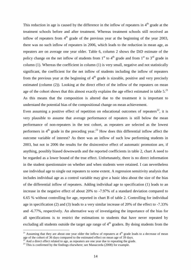
6.2 Interpretation of the results and the disincentive effect of automatic promotion

To understand the ex-ante treatment effect of grade retention, one needs to understand how

this effect is related to the incentive to exert effort. In table 3, column 1 reports the

difference-in-difference estimates of the treatment on repetition rates for grades 1-4. This is

done by following the theoretical exam cohorts of 2003 and 2006 over grades 1-4. The

bottom entry for column 1 shows how the introduction of automatic promotion reduces the

repetition rate in 4th grade by 0.086. Prior to the policy change, about 10% of all students in

treatment schools repeated 4th

grade, but only about 2% did so after the introduction of

automatic promotion.20

In this analysis I am interested in understanding the effect of the drop

of the repetition rate on educational achievement of 4th

graders that arises from the

elimination of the threat of repetition. The two cohorts of students at treatment schools face

very different incentive structures. The 2003 cohort is subject to grade retention, while the

2006 cohort does not face the threat of potential grade retention. For the interpretation of the

estimates as disincentive effect, any possible channel of effects of the policy reform on

outcomes - other then the disincentive effect - has to be precluded. Most importantly,

potential changes in the composition of students in treatment and control schools over time

could have an effect on mean educational outcomes that is not due to the change in the setting

of incentives.

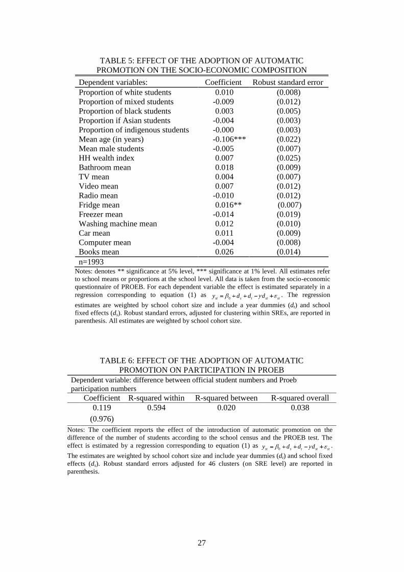
Table 5 reports estimates on a range of mean socioeconomic variables on the school level on

a treatment dummy. For each outcome variable I have fitted a separate regression including

school fixed effects and year dummies. Only the coefficients on the mean number of fridges

per household and on mean age are statistically significant. All other indicators of the socio-

economic composition are not affected by the introduction of automatic promotion, which is

reassuring. While the coefficient for the mean number of fridges per household is very small

and may be due to some spurious correlation, the significant reduction in mean age by about

one month is more relevant and it is important to understand the source of this reduction in

age and its consequence for the interpretation of the result.

20

Repetition rates stay above zero because repetition is still possible when failing to achieve 75% minimum

school attendance.

14

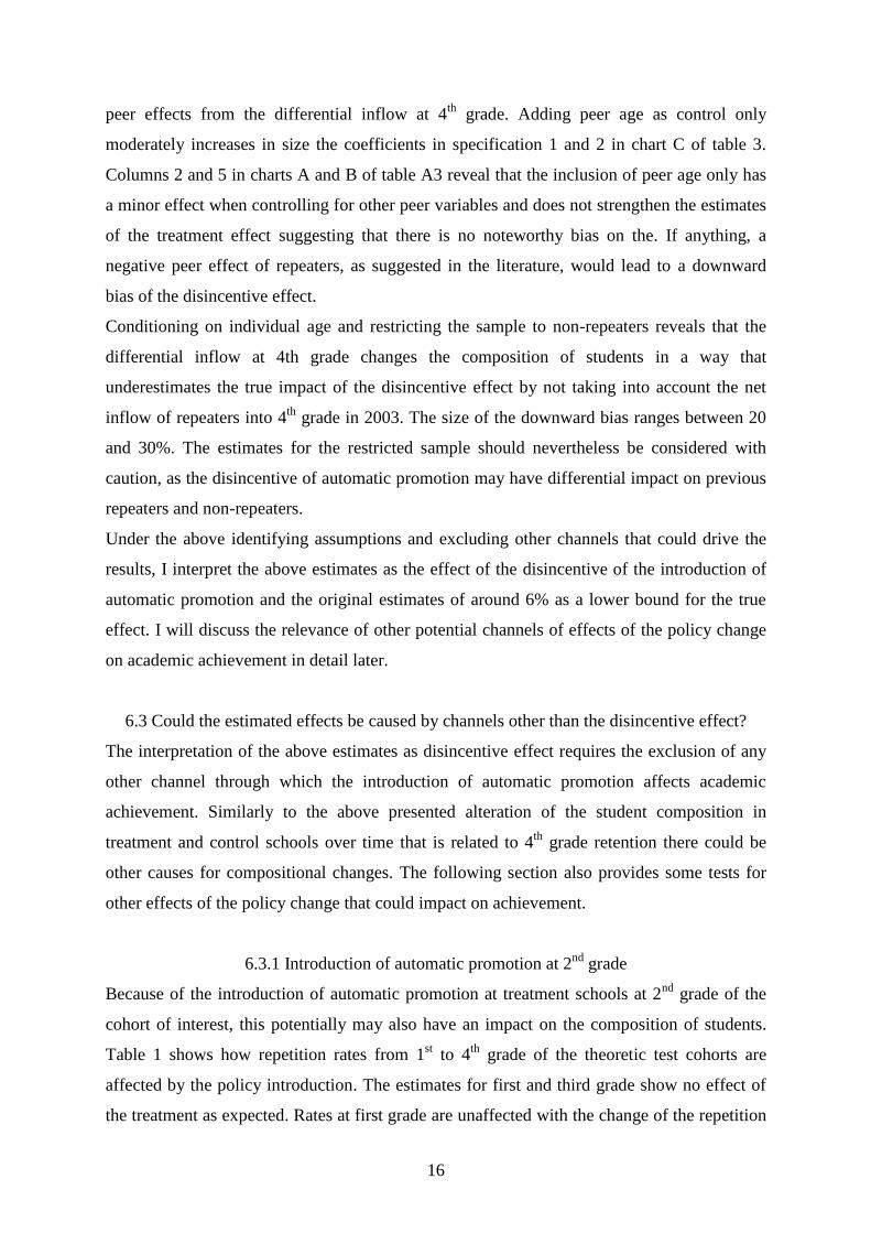
This reduction in age is caused by the difference in the inflow of repeaters in 4th

grade at the

treatment schools before and after treatment. Whereas treatment schools still received an

inflow of repeaters from 4th

grade of the previous year at the beginning of the year 2003,

there was no such inflow of repeaters in 2006, which leads to the reduction in mean age, as

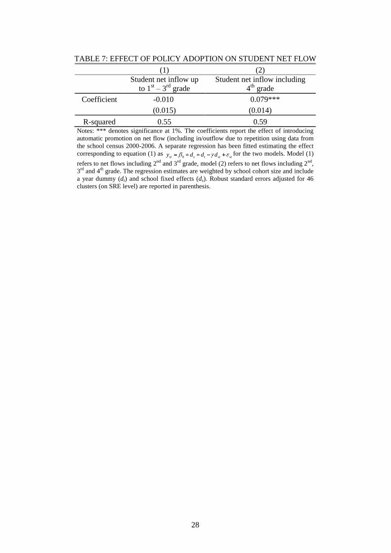
repeaters are on average one year older. Table 6, column 2 shows the DiD estimate of the

policy change on the net inflow of students from 1st to 4

th grade and from 1

st to 3

rd grade in

column (1). Whereas the coefficient in column (1) is very small, negative and not statistically

significant, the coefficient for the net inflow of students including the inflow of repeaters

from the previous year at the beginning of 4th

grade is sizeable, positive and very precisely

estimated (column (2)). Looking at the direct effect of the inflow of the repeaters on mean

age of the cohort shows that this almost exactly explains the age effect estimated in table 5.21

As this means that the composition is altered due to the treatment it is important to

understand the potential bias of the compositional change on mean achievement.

Even assuming a positive effect of repetition on educational outcomes of repeaters22

, it is

very plausible to assume that average performance of repeaters is still below the mean

performance of non-repeaters in the test cohort, as repeaters are selected as the lowest

performers in 4th

grade in the preceding year.23

How does this differential inflow affect the

outcome variable of interest? As there was an inflow of such low performing students in

2003, but not in 2006 the results for the disincentive effect of automatic promotion are, if

anything, possibly biased downwards and the reported coefficients in table 2, chart A need to

be regarded as a lower bound of the true effect. Unfortunately, there is no direct information

in the student questionnaire on whether and when students were retained. I can nevertheless

use individual age to single out repeaters to some extent. A regression sensitivity analysis that

includes individual age as a control variable may give a basic idea about the size of the bias

of the differential inflow of repeaters. Adding individual age to specification (1) leads to an

increase in the negative effect of about 20% to -7.97% of a standard deviation compared to

6.65 % without controlling for age, reported in chart B of table 2. Controlling for individual

age in specification (2) and (3) leads to a very similar increase of 20% of the effect to -7.33%

and -6.77%, respectively. An alternative way of investigating the importance of the bias for

all specifications is to restrict the estimations to students that have never repeated by

excluding all students outside the target age range of 4th

graders. By doing students from the

21

Assuming that they are about one year older the inflow of repeaters at 4th

grade leads to a decrease of mean

age of the cohort of 36 days compared to the estimated effect on mean age of 39 days. 22

And a direct effect related to age, as repeaters are one year due to repeating the grade. 23

This is confirmed by the findings elsewhere; see Manacorda (2008) for example.

15

additional inflow at 4th

grade from the sample are removed, leaving a sample with students

that have never repeated.24

Chart A of table 4 reports the results for the same specifications as

in table 3, but restricts the sample to students in the target age range for 4th

graders. By

restricting the sample in this way the coefficients exceed the estimates of the original full

sample in all specifications by around 30%. The estimated effect is a further 11-16% larger

compared to the estimates in chart B of table 2. Restricting the sample to repeaters (chart B,

table 4) reveals a negative effect that is considerably smaller and no longer statistically

significant. The number of excluded students is nevertheless larger than what could be

explained by excluding 4th

grade repeaters only. Removing overage students from the sample

also removes students that have repeated at 3rd

grade. As repetition is equally possible in all

schools at 3rd

grade, the additional increase in the estimates is therefore not necessarily

related to treatment. The increase rather suggests that the incentive of grade retention may

have a different impact on previous repeaters compared to students that have never repeated a

grade. The cost of repetition is likely highest for students that have not previously repeated.

In contrast marginal cost of being retained again is diminishing for previous repeaters, as they

may already have suffered stigmatization and have already been separated from their original

peer group. The difference in results for the restricted sample therefore may not only reflect

the correction for the differential inflow of repeaters at 4th

grade, but may also more generally

reflect heterogeneous effects on repeaters and non-repeaters.

A more comprehensive analysis of the sensitivity of the estimates to the inclusion of age

controls is provided by table A3 in the annex. I present different specifications of equation (1)

with and without controlling for individual age for the full sample (chart A) and the age

restricted sample in chart B. The results support the previous findings. Adding individual age

as control (columns 4, 6 and 8) strengthens the negative effect in the full and restricted

sample for all the different specifications.

Besides the direct effect on the composition, there may be indirect effects of having repeaters

in the class room on their peers. Repeaters may impose a negative externality on their peers

because their achievement is lower or because they may be more disruptive in class. Lavy,

Paserman and Schlosser (2011) elaborate on the extent of ability peer effects associated with

repeaters and show that academic performance and behaviour of repeaters may be responsible

for the negative effect. By adding peer age in the DiD specification I can control for potential

24

Nevertheless I cannot distinguish repeaters from students that have enrolled late at first grade. With rather

strict enforcement of the enrolment age in Minas Gerais and the incentives to parents to enrol their children

based on Bolsa Família conditions, late enrolment is very limited.

16

peer effects from the differential inflow at 4th

grade. Adding peer age as control only

moderately increases in size the coefficients in specification 1 and 2 in chart C of table 3.

Columns 2 and 5 in charts A and B of table A3 reveal that the inclusion of peer age only has

a minor effect when controlling for other peer variables and does not strengthen the estimates

of the treatment effect suggesting that there is no noteworthy bias on the. If anything, a

negative peer effect of repeaters, as suggested in the literature, would lead to a downward

bias of the disincentive effect.

Conditioning on individual age and restricting the sample to non-repeaters reveals that the

differential inflow at 4th grade changes the composition of students in a way that

underestimates the true impact of the disincentive effect by not taking into account the net

inflow of repeaters into 4th

grade in 2003. The size of the downward bias ranges between 20

and 30%. The estimates for the restricted sample should nevertheless be considered with

caution, as the disincentive of automatic promotion may have differential impact on previous

repeaters and non-repeaters.

Under the above identifying assumptions and excluding other channels that could drive the

results, I interpret the above estimates as the effect of the disincentive of the introduction of

automatic promotion and the original estimates of around 6% as a lower bound for the true

effect. I will discuss the relevance of other potential channels of effects of the policy change

on academic achievement in detail later.

6.3 Could the estimated effects be caused by channels other than the disincentive effect?

The interpretation of the above estimates as disincentive effect requires the exclusion of any

other channel through which the introduction of automatic promotion affects academic

achievement. Similarly to the above presented alteration of the student composition in

treatment and control schools over time that is related to 4th

grade retention there could be

other causes for compositional changes. The following section also provides some tests for

other effects of the policy change that could impact on achievement.

6.3.1 Introduction of automatic promotion at 2nd

grade

Because of the introduction of automatic promotion at treatment schools at 2nd

grade of the

cohort of interest, this potentially may also have an impact on the composition of students.

Table 1 shows how repetition rates from 1st to 4

th grade of the theoretic test cohorts are

affected by the policy introduction. The estimates for first and third grade show no effect of

the treatment as expected. Rates at first grade are unaffected with the change of the repetition

17

regime only in the subsequent year and third grade rates are unaffected as the final year of the

cycle (3rd

grade) remains with grade retention for both cohorts in treatment and control group.

The estimate for the impact on the second grade reveals how the policy introduction lowers

the repetition rate by almost 12% at second grade in 2004. The potential threat to the

interpretation of the results arises from the fact that by introducing automatic promotion at 2nd

grade for the 2006 exam cohort, this cohort may be “contaminated” by low performers that

would have been removed in the absence of treatment. The mean repetition rate for 2nd

grade

at treatment schools drops from 12.8% (2003 exam cohort) to 3.1% (treatment cohort).

Rather then looking at 2nd

grade repetition only, in- and outflows in each grade up to the end

of 3rd

grade have to be taken into account when examining the effect of the adoption of

automatic promotion on the student composition. Looking at the overall student flows of the

text cohorts reveals that the negative selection has largely cancelled out up to when the test

cohort enters 4th

grade in 2006. In particular, repetition at the consecutive 3rd

grade plays an

important role here. The first column of table 7 reports the effect of the policy introduction on

the net flow taking into account in- and outflows over grades 1-3. The net inflow due to the

introduction of automatic promotion is very close to zero and not statistically significant. This

is mainly based on two factors: Focussing only on treatment schools, table A4 shows that

repetition rates at 3rd

grade actually increased by about 4.3% for the 2006 exam cohort, which

filters out a substantive fraction of the low-performers already. Furthermore, 3rd

grade

repetition rates for the two cohorts have to be compared with caution, as these may have a

different impact on removing low-performers from the previous year depending on the inflow

into 3rd grade at the beginning of the year. Considering net-flows, the 2003 and 2006 cohorts

are nearly unaffected in terms of their composition at the beginning of 4th

grade. As

mentioned earlier, the socioeconomic composition between the cohorts (table 5) is almost

completely unaltered due to treatment, which supports the findings, that the policy

introduction does not change the composition of students up to 4th

grade.

This is also corroborated by the fact that almost the entire fraction of the DiD result arises

from the ex-ante difference between treatment and control group in 2003, rather than from

the difference after treatment. The results for the simple difference over time of the control

schools and the difference between control and treatment schools after treatment in 2006 are

very small and not significant at conventional levels.

18

6.3.2 Effect of the policy change on drop-out rates

Elsewhere in the literature the effect of retention on student drop-out has been studied how

(see Jacob and Lefgren 2004, 2009, Manacorda 2011). If the introduction of automatic

promotion has an effect on drop-out rates in grades prior to 4th

grade, this may change

unobserved student characteristics that cannot be controlled for. To test for an effect of the

policy change on drop-out rates I estimate its effect on drop-out rates in a DiD specification

similar to equation (1) as 0s t s t s t s ty d d d (2) using aggregated data from

schools. Column (2) of table 3 reports the coefficients for each grade. Drop-out rates in 2nd

grade are unaffected by the policy change.25

The treatment nevertheless has a small effect on

drop-out rates at 3rd

grade, by reducing the drop-out rate by half a percent. This is equivalent

to a mean reduction of 0.31 students per school/cohort and presumably negligible in its

potential impact on student outcomes.

6.3.3 Effect of the policy change on school transfer rates

Another potential source for a compositional change is related to the possibility of students to

change their school. Parents expecting a negative effect of automatic promotion on their

children may want to move their children to a school with grade retention. In Minas Gerais

the possibility for switching public schools is very limited, as enrolment is based on residence

and parents cannot choose freely between different public schools. Given very substantial

fees at private schools it is also unlikely that parents move their child to a private school to

circumvent a specific grade promotion regime. To test for any effect of the policy change on

between-school mobility I estimate the effect of the policy adoption on student transfer rates

using the same framework as in the previous section. Column (3) of table 3 shows that there

is no significant effect of the regime change on transfer rates for any grade including grades

2, 3 and 4, and an effect of differential student mobility on the outcome variable can be ruled-

out.

6.3.4 Systematic test taking behaviour

Although participation in PROEB is mandatory on the school and individual level, some

students fail to attend the test.26

If the propensity to show up at the exam is related to the

25

1st grade repetition rates are also unaffected as predicted, because the policy change only takes effect after 1

st

grade. This is a relevant observation as it shows that there are no anticipatory effects from schools to the

introduction to the policy change. 26

The participation rate for the 2003 and 2006 wave of PROEB is around 95% as participation is strictly

enforced and absence is only permitted in case of illness.

19

capacity of the student and to the treatment status of the school, this might bias the estimates.

This might be induced by strategic behaviour of school administrators or teachers trying to

manipulate the mean test scores of their school in the PROEB exam. If this is systematically

linked to treatment status this could bias the estimates. I use information from the official

student numbers in each school from the school census and compare these to the number of

students participating in PROEB. I estimate the above regression (2) using the difference

between the two figures as outcome variable. Column (4) of table 3 presents the results from

the regression. The coefficients are very small (.12 students) and are not significant so that

there is no evidence for systematic absence from the exam or manipulation by schools related

to treatment status.

6.3.5 Effect of the policy change on class size

Besides compositional effects the potential reallocation of resources within schools that are

induced by the policy change need to be considered. With a reduction in retention rates,

class-size may be affected. There is a comprehensive literature on the effect of class size on

student performance and the overall picture about class-size effects remains rather unclear.27

To rule out that the estimates are biased by an indirect effect of the policy on class-size I test

for an effect of treatment on class-size for each grade for the cohort of interest in the above

framework. Column (4) of table 3 reports the results for the DiD regressions. There is no

significant effect of the policy change on class-size in any grade, so that estimates on test

scores are unlikely biased by effects of the treatment on class-size.

Even under the assumption that the introduction of automatic promotion releases other school

resources that could be allocated to 4th

grade students (for which there is no evidence in the

present analysis) this would lead to underestimating the true impact of the disincentive

created by automatic promotion.

The fact that none of the above estimates (for repetition rates, drop-out rates, class-size,

transfer rates) reveal any significant effect for first grade estimates is in itself an important

falsification exercise. All these estimates are based on a pseudo-treatment as the first grade of

the 2006 exam cohort was not yet affected by the policy introduction that took place only at

2nd

grade. This also shows that there are no anticipatory effects of the schools in respect to the

imminent introduction of automatic promotion that may affect student outcomes at a later

stage.

27

See Hoxby (2000) and Angrist & Lavy (1999) for two prominent studies on class size effects.

20

7. CONCLUSIONS

Existing empirical work on grade retention has to date focused on analysing the direct effect

of retention on repeaters. The focus on the ex-post effect may nevertheless neglect an

important effect of the grade retention regime on incentives to exert effort on a much larger

range of students. The introduction of automatic promotion removes the incentive previously

linked to the threat of retention and I use exogenous variation in the implementation of the

policy over time in state primary schools in the Brazilian state of Minas Gerais to obtain

causal estimates of the disincentive effect from the introduction of automatic promotion

measured by the impact on standardized math test scores.

Using a difference-in-difference approach I find a negative effect of 0.06 of a standard

deviation, significant at the 1% level. Controlling for individual age strengthens the negative

effect by about 20%, which gives an idea about the size of the bias associated with the

differential inflow of repeaters into 4th

grade before and after treatment.

The estimated disincentive effect of the introduction of automatic promotion appears to be of

moderate size. Considering the potential for an accumulative nature of the negative effect

over several grades, the overall impact of the automatic promotion regime may lead to

considerable loss of academic achievement over the eight years of primary school.

The estimates of the disincentive effect related to removing the deterrent of repetition close a

gap in the literature on the effects of grade retention and help to explain the persistence of

repetition regimes in many countries. Grade retention reduces internal flow efficiency at

schools and is a costly policy, but creates a positive effect on academic achievement through

the deterrence of retention. The findings are also important because they reveal that a large

fraction of students is affected by the grade promotion regime. Rather than focusing only on

the effect on repeaters, attempts to assess the cost and benefit of retention therefore need to

take into account as well the effects on non-repeaters.

The results are particularly relevant because of the universal introduction of automatic

promotion in all primary schools in Brazil coming into effect by federal legislation in 2011.

Although the Brazilian experience may not be completely transferable to other countries with

often lower repetition rates, the findings may nevertheless be relevant for the discussion of

automatic promotion, often referred to as social promotion in the United States, in these

countries and may provide policy makers with a more complete picture of the potential

effects of changes in the repetition regime.

8. LITERATURE

Angrist, Joshua D. and Victor Lavy. 2009. “The Effect of High Stakes High School

Achievement Awards: Evidence from a Group-Randomized Trial.” American Economic Review,

99(4): 1384-1414.

Angrist, Joshua D., Eric Bettinger, Erik Bloom, Elizabeth King and Michael Kremer. 2002.

“Vouchers for Private Schooling in Colombia: Evidence from Randomized Natural

Experiments.” American Economic Review, 92(5): 1535-1558.

Angrist, Joshua D., Eric Bettinger and Michael Kremer. 2006. “Long-term Consequences of

Secondary School Vouchers: Evidence from Administrative Records in Columbia.” American

Economic Review, 96(3): 847-862.

Angrist, Joshua D. and Victor Lavy. 1999. “Using Maimonides‟ Rule to Estimate the Effect of

Class Size on Scholastic Achievement.” Quarterly Journal of Economics. 114(2): 533-575.

Ashenfelter, Orley. 1978. “Estimating the Effect of Training Programs on Earnings.”

Review of Economics and Statistics, 60(1): 47-57.

Corman, Hope. 2003. “The Effects of State Policies, Individual Characteristics, Family

Characteristics, and Neighbourhood Characteristics on Grade Retention in the United States.”

Economics of Education Review, 22: 409-420.

De Janvry, Alain, Frederico Finan and Elisabeth Sadoulet. 2006. “Evaluating Brazil‟s Bolsa

Escola Program: Impact on Schooling and Municipal Roles.” Unpublished manuscript.

De Mello, Luiz and Mombert Hoppe. 2005. “Education Attainment in Brazil: the Experience of

FUNDEF.” OECD Economics Department Working Papers 424.

Donald, Stephen and Kevin Lang. 2007. “Inference with Differences-in-Differences and Other

Panel Data.” Review of Economics and Statistics, 89: 221-233.

Dong, Yingying. 2009. “Kept Back to Get Ahead? Kindergarten Retention and Academic

Performance.” European Economic Review, 54(2): 219-236.

Dynarski, Susan. 2003. “Does Aid Matter? Measuring the Effect of Student Aid on College

Attendance and Completion.” American Economic Review, 93(1): 279-288.

Eide, Eric and Mark Showalter. 2001. “The Effect of Grade Retention on Educational and Labor

Market Outcomes.” Economics of Education Review, 20(6): 563-576.

Ferrão, Maria Eugênia, Kaizô lwakami Beltrão and Denis Paulo dos Santos. 2002. “O Impacto

de Políticas de Não-Repetência sobre o Aprendizado dos Alunos da Quarta Série.” Pesquisa e

Planejamento Econômico, 32(3): 495-514.

Glick, Peter, and David Sahn. “Early Academic Performance, Grade Repetition, and School

Attainment in Senegal: A Panel Data Analysis.” The World Bank Economic Review, 24(1): 93-

120.

22

Gomes-Neto, João B. and Eric A. Hanushek. 1994. “Causes and Consequences of Grade

Retention: Evidence from Brazil.” Economic Development and Cultural Change, 43(1): 117-48.

Henry, Gary T. and Ross Rubinstein. 2001. “Paying for Grades: Impact of Merit-Based

Financial Aid on Educational Quality.” Journal of Policy Analysis and Management, 21(1): 93-

109.

Holmes, Thomas C. 1989. “Grade Level Retention Effects: A Meta-Analysis of Research

Studies.” In: Flunking Grades: Research and Policies on Retention, ed. Lorrie A. Shepard and

Mary L. Smith, 16-33. London: Falmer Press.

IBGE (Brazilian Institute of Geography and Statistics). 2007. “Contas Nacionais No. 21: Contas

Regionais do Brasil 2002-2005.” Rio de Janeiro.

Imbens, Guido and Jeffrey Wooldridge. 2009. “Recent Developments in the Econometrics of

Program Evaluation.” Journal of Economics Literature, 47(1): 5–86.

INEP (National Institute for Educational Studies and Research). 2007. “IDEB - Prova

Brasil/Saeb 2007.” Brasilia.

Jacob, Brian A. 2005. “Accountability, Incentives and Behaviour: Evidence from School

Reform in Chicago.” Journal of Public Economics, 89(5-6): 761-796.

Jacob, Brian and Lars Lefgren. 2004. “Remedial Education and Student Achievement: a

Regression-Discontinuity Analysis.” Review of Economics and Statistics, 86(1): 226-44.

Jacob, Brian and Lars Lefgren. 2009. “The Effect of Grade Retention on High School

Completion.” American Economic Journal: Applied Economics, 1(3): 33-58.

Kremer, Michael, Edward Miguel and Rebecca Thornton. 2009. “Incentives to Learn.” Review

of Economics and Statistics, 91(3): 437-56.

Lavy, Victor, Daniele Paserman and Analia Schlosser. 2011. “Inside the Black Box of Ability

Peer Effects: Evidence from Variation in Low Achievers in the Classroom.” Economic Journal,

forthcoming.

Lazear, Edward P. and Michael Gibbs. 2007. “Personnel Economics in Practice.” 2nd

ed. Wiley,

Hoboken.

Lindert, Kathy, Anja Linder, Jason Hobbs and Bénédict de la Brière. 2007. “The Nuts and Bolts

of Brazil‟s Bolsa Família Program: Implementing Conditional Cash Transfers in a Decentralized

Context.” Social Protection Discussion Paper 0709, World Bank.

Mainardes, Jefferson. 2004. “Moving Away from a Graded System: a Policy Analysis of the

Cycles of Learning Project (Brazil).” Unpublished manuscript.

Manacorda, Marco. 2011. “The Cost of Grade Retention.” Review of Economics and Statistics,

forthcoming.

23

MEC (Brazilian Ministry of Education). 1996. “Lei de Diretrizes e Bases da Educação

National, No. 9394, Art. 24, December 1996, Brasilia.

OECD. 2005. “OECD Economic Survey of Brazil 2005”. Organization for Cooperation and

Development, Paris.

Schultz, Paul T. 2004. “School Subsidies for the Poor: Evaluating the Mexican Progresa Poverty

Program.” Journal of Development Economics, 74(1): 199-250.

Pino, Ivany R. and Mariane C. Koslinki. 1999. “Government Programs to Eliminate Repetition,

School Dropout and Exclusion in Brazil.” In: Schooling for Success: Preventing Repetition and

Dropout in Latin American Primary Schools, ed. Laura Randall and Joan B. Anderson. New

York: Sharpe.

UNESCO. 2008. “EFA Global Monitoring Report.” United Nations Educational,

Scientific and Cultural Organization, Paris.

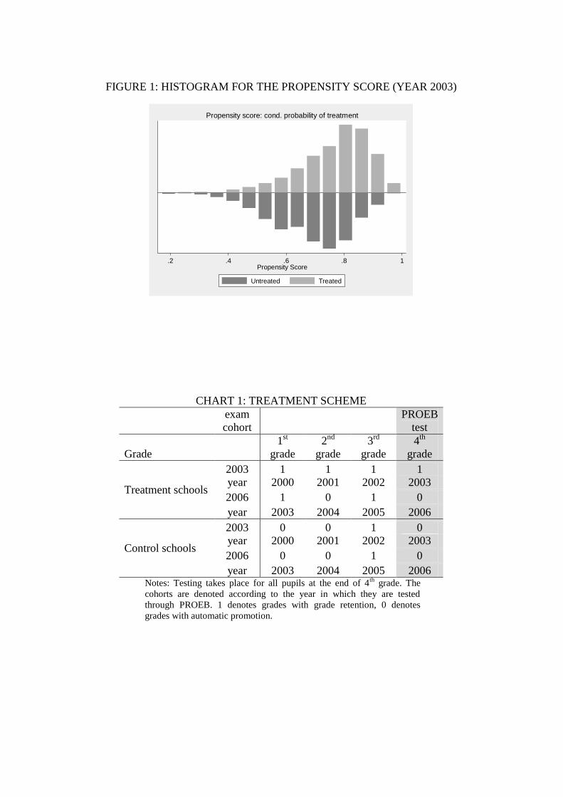
FIGURE 1: HISTOGRAM FOR THE PROPENSITY SCORE (YEAR 2003)

.2 .4 .6 .8 1Propensity Score

Untreated Treated

Propensity score: cond. probability of treatment

CHART 1: TREATMENT SCHEME

exam

cohort

PROEB

test

Grade

1st

grade

2nd

grade

3rd

grade

4th

grade

Treatment schools

2003 1 1 1 1

year 2000 2001 2002 2003

2006 1 0 1 0

year 2003 2004 2005 2006

Control schools

2003 0 0 1 0

year 2000 2001 2002 2003

2006 0 0 1 0

year 2003 2004 2005 2006 Notes: Testing takes place for all pupils at the end of 4

th grade. The

cohorts are denoted according to the year in which they are tested

through PROEB. 1 denotes grades with grade retention, 0 denotes

grades with automatic promotion.

25

TABLE 1: TEST SCORE MEANS IN TREATMENT AND CONTROL SCHOOLS

BEFORE AND AFTER THE ADOPTION IN THE TREATMENT SCHOOLS

Before treatment After treatment Change in mean

test scores

Control schools 498.48 498.99 -0.51

(1.55) (1.51) (2.01)

Treatment schools 505.53 499.39 6.14

(2.71) (2.59) (2.97)

Difference in mean test

scores

-7.05

(3.12)

-0.40

(2.99)

-6.65

(3.22) Notes: Mean outcomes for treatment and control before and after treatment. Standard errors, adjusted for

clustering within SREs, are reported in parenthesis.

TABLE 2: MAIN ESTIMATION RESULTS AND SENSITIVITY TO AGE

CONTROLS

Dependent variable: PROEB math test scores

Observations: 244,081, number of clusters: 1,993

(1) (2) (3) (4)

Chart A

Treatment effect -6.65*** -6.13*** -5.67*** -6.24***

(2.03) (2.00) (1.98) (2.04)

R-squared 0.00 0.01 0.01 0.17

Chart B – adding individual age control

Treatment effect

-7.97***

(2.16)

-7.33***

(2.11)

-6.77***

(2.04)

-6.24***

(2.04)

R-squared 0.05 0.04 0.04 0.17

Chart C – adding peer age control

Treatment effect

-6.99***

(2.06)

-6.46***

(2.02)

-5.67***

(1.98)

-6.24***

(2.04)

R-squared 0.00 0.01 0.01 0.17

School fixed effects

Year dummies

yes

yes

yes

yes

yes

yes

yes

yes

School level controls no yes yes yes

Peer characteristics controls no no yes yes

Individual characteristics controls no no no yes Notes: *** denotes significance at 1%. Robust standard errors, adjusted for clustering

within schools, are reported in parenthesis. Specification (1) contains year dummies and

school fixed effects, specification (2) additionally controls for a rich set of school

characteristics (physical characteristics of the school and the class rooms, teaching

material, teacher characteristics, participation in educational programmes etc.),

specification (3) additionally controls for peer socio-economic characteristics at the school

level and specification (4) also controls for individual characteristics.

26

TABLE 3: EFFECT OF THE ADOPTION OF AUTOMATIC

PROMOTION ON STUDENT FLOWS AND CLASS-SIZE

Dependent variable:

Repetition rate

(1)

Drop-out rate

(2)

Transfer-rate

(3)

Class-size

(4)

Grade 1 -0.010 0.001 -0.005 0.692

(0.010) (0.003) (0.007) (0.363)

Grade 2 -0.118*** -0.002 0.002 0.828

(0.010) (0.003) (0.006) (0.422)

Grade 3 -0.019 -0.005** -0.002 0.502

(0.011) (0.002) (0.003) (0.416)

Grade 4 -0.086*** -0.005 -0.007 0.252

(0.007) (0.004) (0.004) (0.336)

Number of schools: 1993, years 2000-2006, average cohort size: 61.24 Notes: *** denotes significance at 1%, ** denotes significance at 5%. The

coefficients report the effect of introducing automatic promotion on the dependent

variables for 1st to 4

th grade using data from the school census 2000-2006 following

the theoretical test cohorts. For each grade a separate regression has been fitted

estimating the effect corresponding to equation (1) as0st s t st sty d d d . The

regression estimates are weighted by school cohort size and include year dummies

(dt) and school fixed effects (ds). Robust standard errors, adjusted for clustering

within 46 SREs, are reported in parenthesis.

TABLE 4: ESTIMATION RESULTS FOR RESTRICTED AGE RANGES

Dependent variable: PROEB test scores

Number of clusters: 1,993

(1) (2) (3) (4)

Chart A – students in target age range for 4th

grade

Treatment effect -8.67*** -8.07*** -7.50*** -7.22***

(2.33) (2.26) (2.23) (2.25)

R-squared 0.00 0.01 0.01 0.13

Observations 149,223

Chart B – repeaters (outside target age range)

Treatment effect -3.78 -3.42 -2.89 -3.29

(2.53) (2.50) (2.50) (2.42)

R-squared 0.01 0.01 0.00 0.08

Observations 88,657

School fixed effects

Year dummy

yes

yes

yes

yes

yes

yes

yes

yes

School level controls no yes yes yes

Peer characteristics controls no no yes yes

Individual characteristics controls no no no yes Notes: *** denotes significance at 1%. The above samples exclude students that are below the target

age range. Robust standard errors, adjusted for clustering within schools, are reported in parenthesis.

Specification (1) only includes year dummies and school fixed effects, specification (2) additionally

controls for a rich set of school characteristics (physical characteristics of the school and the class

rooms, teaching material, teacher characteristics, participation in educational programmes etc.),

specification (3) additionally controls for peer socio-economic characteristics at the school level and

specification (4) also controls for individual characteristics.

27

TABLE 5: EFFECT OF THE ADOPTION OF AUTOMATIC

PROMOTION ON THE SOCIO-ECONOMIC COMPOSITION

Dependent variables: Coefficient Robust standard error

Proportion of white students 0.010 (0.008)

Proportion of mixed students -0.009 (0.012)

Proportion of black students 0.003 (0.005)

Proportion if Asian students -0.004 (0.003)

Proportion of indigenous students -0.000 (0.003)

Mean age (in years) -0.106*** (0.022)

Mean male students -0.005 (0.007)

HH wealth index 0.007 (0.025)

Bathroom mean 0.018 (0.009)

TV mean 0.004 (0.007)

Video mean 0.007 (0.012)

Radio mean -0.010 (0.012)

Fridge mean 0.016** (0.007)

Freezer mean -0.014 (0.019)

Washing machine mean 0.012 (0.010)

Car mean 0.011 (0.009)

Computer mean -0.004 (0.008)

Books mean 0.026 (0.014)

n=1993 Notes: denotes ** significance at 5% level, *** significance at 1% level. All estimates refer

to school means or proportions at the school level. All data is taken from the socio-economic

questionnaire of PROEB. For each dependent variable the effect is estimated separately in a

regression corresponding to equation (1) as 0st s t st sty d d d . The regression

estimates are weighted by school cohort size and include a year dummies (dt) and school

fixed effects (ds). Robust standard errors, adjusted for clustering within SREs, are reported in

parenthesis. All estimates are weighted by school cohort size.

TABLE 6: EFFECT OF THE ADOPTION OF AUTOMATIC

PROMOTION ON PARTICIPATION IN PROEB

Dependent variable: difference between official student numbers and Proeb

participation numbers

Coefficient R-squared within R-squared between R-squared overall

0.119 0.594 0.020 0.038

(0.976)

Notes: The coefficient reports the effect of the introduction of automatic promotion on the

difference of the number of students according to the school census and the PROEB test. The

effect is estimated by a regression corresponding to equation (1) as 0st s t st sty d d d .

The estimates are weighted by school cohort size and include year dummies (dt) and school fixed

effects (ds). Robust standard errors adjusted for 46 clusters (on SRE level) are reported in

parenthesis.

28

TABLE 7: EFFECT OF POLICY ADOPTION ON STUDENT NET FLOW

(1) (2)

Student net inflow up

to 1st – 3

rd grade

Student net inflow including

4th

grade

Coefficient -0.010 0.079***

(0.015) (0.014)

R-squared 0.55 0.59 Notes: *** denotes significance at 1%. The coefficients report the effect of introducing

automatic promotion on net flow (including in/outflow due to repetition using data from

the school census 2000-2006. A separate regression has been fitted estimating the effect

corresponding to equation (1) as 0st s t st sty d d d for the two models. Model (1)

refers to net flows including 2nd

and 3rd

grade, model (2) refers to net flows including 2nd

,

3rd

and 4th

grade. The regression estimates are weighted by school cohort size and include

a year dummy (dt) and school fixed effects (ds). Robust standard errors adjusted for 46

clusters (on SRE level) are reported in parenthesis.

29

9. ANNEX

TABLE A1: MEAN CHARACTERISTICS OF TREATMENT AND CONTROL GROUPS IN 2003 AND 2006

CHART A: PHYSICAL CHARACTERISTICS AND SCHOOL PROGRAMME PARTICIPATION

2003 2006

Control Treatment Control Treatment

n=1993 Mean SD Mean SD P-value

Norm-

diff Mean SD Mean SD P-value

Norm-

diff

Rural school 0.885 (0.319) 0.890 (0.313) 0.788 -0.011 0.885 (0.319) 0.895 (0.307) 0.544 -0.023

State property 0.918 (0.275) 0.880 (0.325) 0.020 0.089 0.907 (0.290) 0.881 (0.324) 0.106 0.060

Municipal property 0.062 (0.242) 0.093 (0.290) 0.035 -0.082 0.066 (0.249) 0.090 (0.287) 0.098 -0.063

Private property 0.020 (0.141) 0.067 (0.161) 0.414 -0.220 0.024 (0.154) 0.027 (0.163) 0.696 -0.013

School ownership 0.901 (0.298) 0.866 (0.340) 0.040 0.077 0.907 (0.290) 0.881 (0.324) 0.106 0.060

Rented school 0.014 (0.118) 0.020 (0.140) 0.393 -0.033 0.010 (0.100) 0.09 (0.138) 0.164 -0.469

Donated school 0.085 (0.278) 0.114 (0.317) 0.068 -0.069 0.082 (0.275) 0.100 (0.300) 0.261 -0.044

Shared school 0.197 (0.398) 0.238 (0.426) 0.060 -0.070 0.197 (0.398) 0.197 (0.398) 10.00 0.000

Principal office 0.875 (0.331) 0.858 (0.350) 0.324 0.035 0.865 (0.342) 0.874 (0.332) 0.625 -0.019

Admin. office 0.909 (0.287) 0.937 (0.243) 0.036 -0.074 0.950 (0.219) 0.952 (0.214) 0.845 -0.007

Teacher room 0.813 (0.390) 0.811 (0.392) 0.912 0.004 0.827 (0.379) 0.843 (0.363) 0.382 -0.030

School kitchen 0.829 (0.377) 0.824 (0.381) 0.808 0.009 0.821 (0.384) 0.821 (0.384) 0.997 0.000

Refectory 0.374 (0.484) 0.440 (0.497) 0.010 -0.095 0.412 (0.493) 0.464 (0.499) 0.046 -0.074

Food storage 0.839 (0.368) 0.856 (0.352) 0.368 -0.033 0.732 (0.443) 0.718 (0.450) 0.533 0.022

Computer lab 0.237 (0.426) 0.149 (0.356) 0.000 0.159 0.302 (0.460) 0.193 (0.394) 0.000 0.180

Science lab 0.165 (0.372) 0.142 (0.349) 0.205 0.045 0.143 (0.350) 0.120 (0.325) 0.176 0.048

Other lab 0.022 (0.147) 0.021 (0.145) 0.920 0.005 0.020 (0.141) 0.018 (0.133) 0.767 0.010

Toilets outside 0.054 (0.227) 0.094 (0.291) 0.006 -0.108 0.0443 (0.206) 0.070 (0.254) 0.045 -0.079

Toilets inside 0.980 (0.141) 0.967 (0.178) 0.150 0.057 0.992 (0.089) 0.981 (0.136) 0.101 0.068

Freezer 0.899 (0.301) 0.920 (0.271) 0.144 -0.052 0.907 (0.290) 0.914 (0.280) 0.633 -0.017

Filtered water 0.845 (0.362) 0.825 (0.380) 0.299 0.038 0.881 (0.324) 0.858 (0.350) 0.183 0.048

30

Table A1 cont.

Video cassettes 1.757 (1.000) 1.763 (1.190) 0.911 0.000 1.501 (0.936) 1.551 (1.368) 0.444 -0.030

TV sets 2.038 (1.066) 2.025 (1.324) 0.541 0.024 2.107 (1.021) 2.108 (1.353) 0.980 -0.001

Projectors 0.851 (0.544) 0.858 (0.535) 0.815 -0.009 0.867 (0.545) 0.876 (0.530) 0.741 -0.012

Printers 1.790 (2.200) 1.517 (2.040) 0.002 0.110 2.370 (2.295) 1.948 (1.961) 0.000 0.140

Pentium computers 2.757 (4.866) 1.919 (3.915) 0.000 0.151 3.050 (5.053) 2.239 (4.435) 0.001 0.121

386/486 computers 0.656 (2.486) 0.428 (1.469) 0.014 0.079 1.032 (3.109) 0.737 (2.249) 0.022 0.077

Perm. class rooms 10.069 (4.857) 10.060 (4.343) 0.320 0.035 10.651 (5.439) 10.533 (4.403) 0.625 0.017

Prov. class rooms 0.193 (0.581) 0.150 (0.456) 0.092 0.058 0.165 (0.459) 0.172 (0.516) 0.794 -0.010

Class rooms 9.487 (5.188) 9.205 (4.195) 0.223 0.042 10.010 (5.255) 9.760 (4.198) 0.282 0.037

Total staff 49.535 (30.385) 46.612 (25.796) 0.037 0.073 51.553 (31.624) 48.281 (25.749) 0.021 0.080

Teachers 32.177 (20.045) 30.243 (16.885) 0.035 0.074 32.441 (20.651) 30.207 (16.330) 0.014 0.085

Min inc. program 0.598 (0.491) 0.545 (0.498) 0.043 0.076 0.970 (0.171) 0.967 (0.176) 0.778 0.012

TV escola 0.732 (0.443) 0.751 (0.432) 0.401 -0.031 0.495 (0.500) 0.564 (0.496) 0.008 -0.098

Other education TV 0.237 (0.426) 0.304 (0.460) 0.004 -0.107 0.117 (0.321) 0.150 (0.358) 0.062 -0.069

PROINFO 0.199 (0.400) 0.126 (0.332) 0.000 0.140 0.171 (0.377) 0.124 (0.330) 0.009 0.094

State programmes 0.314 (0.465) 0.206 (0.404) 0.000 0.175 0.247 (0.432) 0.225 (0.418) 0.309 0.037

Munic. programmes 0.091 (0.287) 0.102 (0.303) 0.449 -0.026 0.175 (0.380) 0.170 (0.376) 0.787 0.009

School transport 0.527 (0.500) 0.487 (0.500) 0.118 0.057 0.722 (0.448) 0.668 (0.471) 0.025 0.083

Initial enrolment 72.630 (52.326) 69.245 (50.132) 0.197 0.047 38.276 (30.966) 41.202 (32.187) 0.077 -0.066

Classes in 1st grade 2.537 (1.640) 2.359 (1.542) 0.030 0.079 1.682 (1.259) 1.766 (1.308) 0.215 -0.046

Classes in 2nd

grade 2.410 (1.420) 2.425 (1.581) 0.854 -0.007 1.793 (1.295) 1.963 (1.324) 0.013 -0.092

Classes in 3rd

grade 2.348 (1.428) 2.470 (1.567) 0.125 -0.058 2.163 (1.449) 2.123 (1.420) 0.587 0.020

Classes in 4th

grade 2.334 (1.460) 2.469 (1.571) 0.080 -0.063 2.082 (1.289) 2.076 (1.314) 0.919 0.003 Notes: The binary variables of school characteristics and programme participation are coded 0 for not present (no participation) and 1 for present (participation). All

data is from the Brazilian school census 2003 and 2006. The p-value is reported from a test on the equality of the mean between the treatment and control groups

(independent samples). As the sample size is sufficiently large the result for using a classical t-test or taking into account the binary values and the underlying

binomial distribution deliver very similar results. As the group size and with it the variances between the groups differ, approximate t using individual sample

variances instead of the pooled variance and Welch‟s approximation of the degrees of freedom have been used.

The normalized difference is computed as 1 2

2 2

,0 ,1X X

X Xnorm diff

S S

, where S2 denotes the sample variance of Xi.

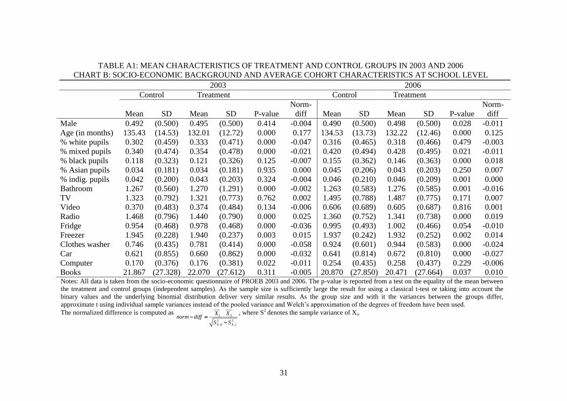
31

TABLE A1: MEAN CHARACTERISTICS OF TREATMENT AND CONTROL GROUPS IN 2003 AND 2006

CHART B: SOCIO-ECONOMIC BACKGROUND AND AVERAGE COHORT CHARACTERISTICS AT SCHOOL LEVEL

2003 2006

Control Treatment Control Treatment

Mean SD Mean SD P-value

Norm-

diff Mean SD Mean SD P-value

Norm-

diff

Male 0.492 (0.500) 0.495 (0.500) 0.414 -0.004 0.490 (0.500) 0.498 (0.500) 0.028 -0.011

Age (in months) 135.43 (14.53) 132.01 (12.72) 0.000 0.177 134.53 (13.73) 132.22 (12.46) 0.000 0.125

% white pupils 0.302 (0.459) 0.333 (0.471) 0.000 -0.047 0.316 (0.465) 0.318 (0.466) 0.479 -0.003

% mixed pupils 0.340 (0.474) 0.354 (0.478) 0.000 -0.021 0.420 (0.494) 0.428 (0.495) 0.021 -0.011

% black pupils 0.118 (0.323) 0.121 (0.326) 0.125 -0.007 0.155 (0.362) 0.146 (0.363) 0.000 0.018

% Asian pupils 0.034 (0.181) 0.034 (0.181) 0.935 0.000 0.045 (0.206) 0.043 (0.203) 0.250 0.007

% indig. pupils 0.042 (0.200) 0.043 (0.203) 0.324 -0.004 0.046 (0.210) 0.046 (0.209) 0.001 0.000

Bathroom 1.267 (0.560) 1.270 (1.291) 0.000 -0.002 1.263 (0.583) 1.276 (0.585) 0.001 -0.016

TV 1.323 (0.792) 1.321 (0.773) 0.762 0.002 1.495 (0.788) 1.487 (0.775) 0.171 0.007

Video 0.370 (0.483) 0.374 (0.484) 0.134 -0.006 0.606 (0.689) 0.605 (0.687) 0.816 0.001

Radio 1.468 (0.796) 1.440 (0.790) 0.000 0.025 1.360 (0.752) 1.341 (0.738) 0.000 0.019

Fridge 0.954 (0.468) 0.978 (0.468) 0.000 -0.036 0.995 (0.493) 1.002 (0.466) 0.054 -0.010

Freezer 1.945 (0.228) 1.940 (0.237) 0.003 0.015 1.937 (0.242) 1.932 (0.252) 0.002 0.014

Clothes washer 0.746 (0.435) 0.781 (0.414) 0.000 -0.058 0.924 (0.601) 0.944 (0.583) 0.000 -0.024

Car 0.621 (0.855) 0.660 (0.862) 0.000 -0.032 0.641 (0.814) 0.672 (0.810) 0.000 -0.027

Computer 0.170 (0.376) 0.176 (0.381) 0.022 -0.011 0.254 (0.435) 0.258 (0.437) 0.229 -0.006

Books 21.867 (27.328) 22.070 (27.612) 0.311 -0.005 20.870 (27.850) 20.471 (27.664) 0.037 0.010 Notes: All data is taken from the socio-economic questionnaire of PROEB 2003 and 2006. The p-value is reported from a test on the equality of the mean between

the treatment and control groups (independent samples). As the sample size is sufficiently large the result for using a classical t-test or taking into account the

binary values and the underlying binomial distribution deliver very similar results. As the group size and with it the variances between the groups differ,

approximate t using individual sample variances instead of the pooled variance and Welch‟s approximation of the degrees of freedom have been used.

The normalized difference is computed as 1 2

2 2

,0 ,1X X

X Xnorm diff

S S

, where S2 denotes the sample variance of Xi.

32

TABLE A2: MEAN PRE-INTERVENTION REPETITION RATES IN 1997

1997

n=1,993 Control Treatment

Mean SD Mean SD P-value Norm-diff

Pre-treatment repetition rate 1st

grade (1997) 0.08 (0.108) 0.08 (0.106) 0.98 -0.001

Pre-treatment repetition rate 2nd

grade (1997) 0.16 (0.208) 0.17 (0.200) 0.37 -0.034

Pre-treatment repetition rate 3rd

grade (1997) 0.05 (0.053) 0.05 (0.143) 0.63 -0.014

Pre-treatment repetition rate 4th

grade (1997) 0.06 (0.072) 0.06 (0.093) 0.21 -0.044 Notes: All data is from the Brazilian school census 1997. The p-value is reported from a test on the equality of the mean

between the treatment and control groups (independent samples). As the sample size is sufficiently large the result for

using a classical t-test or alternatively taking into account the binary values and the underlying binomial distribution

deliver very similar results. As the group size and with it the variances between the groups differ, approximate t using

individual sample variances instead of the pooled variance and Welch‟s approximation of the degrees of freedom have

been used.

The normalized difference is computed as 1 2

2 2

,0 ,1X X

X Xnorm diff

S S

, where S2 denotes the sample variance of Xi.

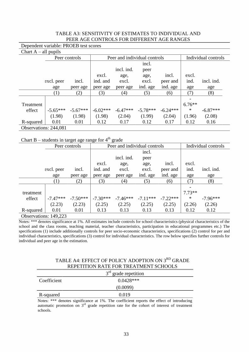
33

TABLE A3: SENSITIVITY OF ESTIMATES TO INDIVIDUAL AND

PEER AGE CONTROLS FOR DIFFERENT AGE RANGES

Dependent variable: PROEB test scores

Chart A – all pupils

Peer controls Peer and individual controls Individual controls

excl. peer

age

incl.

peer age

excl.

ind. and

peer age

incl. ind.

age,

excl.

peer age

incl.

peer

age,

excl.

ind. age

incl.

peer and

ind. age

excl.

ind.

age

incl. ind.

age

(1) (2) (3) (4) (5) (6) (7) (8)

Treatment

effect -5.65*** -5.67*** -6.02*** -6.47*** -5.78*** -6.24***

-

6.76**

* -6.87***

(1.98) (1.98) (1.98) (2.04) (1.99) (2.04) (1.96) (2.08)

R-squared 0.01 0.01 0.12 0.17 0.12 0.17 0.12 0.16

Observations: 244,081

Chart B – students in target age range for 4th

grade

Peer controls Peer and individual controls Individual controls

excl. peer

age

incl.

peer age

excl.

ind. and

peer age

incl. ind.

age,

excl.

peer age

incl.

peer

age,

excl.

ind. age

incl.

peer and

ind. age

excl.

ind.

age

incl. ind.

age

(1) (2) (3) (4) (5) (6) (7) (8)

treatment

effect -7.47*** -7.50*** -7.30*** -7.46*** -7.11*** -7.22***

-

7.73**

* -7.96***

(2.23) (2.23) (2.25) (2.25) (2.25) (2.25) (2.26) (2.26)

R-squared 0.01 0.01 0.13 0.13 0.13 0.13 0.12 0.12

Observations: 149,223 Notes: *** denotes significance at 1%. All estimates include controls for school characteristics (physical characteristics of the

school and the class rooms, teaching material, teacher characteristics, participation in educational programmes etc.) The

specifications (1) include additionally controls for peer socio-economic characteristics, specifications (2) control for per and

individual characteristics, specifications (3) control for individual characteristics. The row below specifies further controls for

individual and peer age in the estimation.

TABLE A4: EFFECT OF POLICY ADOPTION ON 3RD

GRADE

REPETITION RATE FOR TREATMENT SCHOOLS

3rd

grade repetition

Coefficient 0.0428***

(0.0099)

R-squared 0.019 Notes: *** denotes significance at 1%. The coefficient reports the effect of introducing

automatic promotion on 3rd

grade repetition rate for the cohort of interest of treatment

schools.

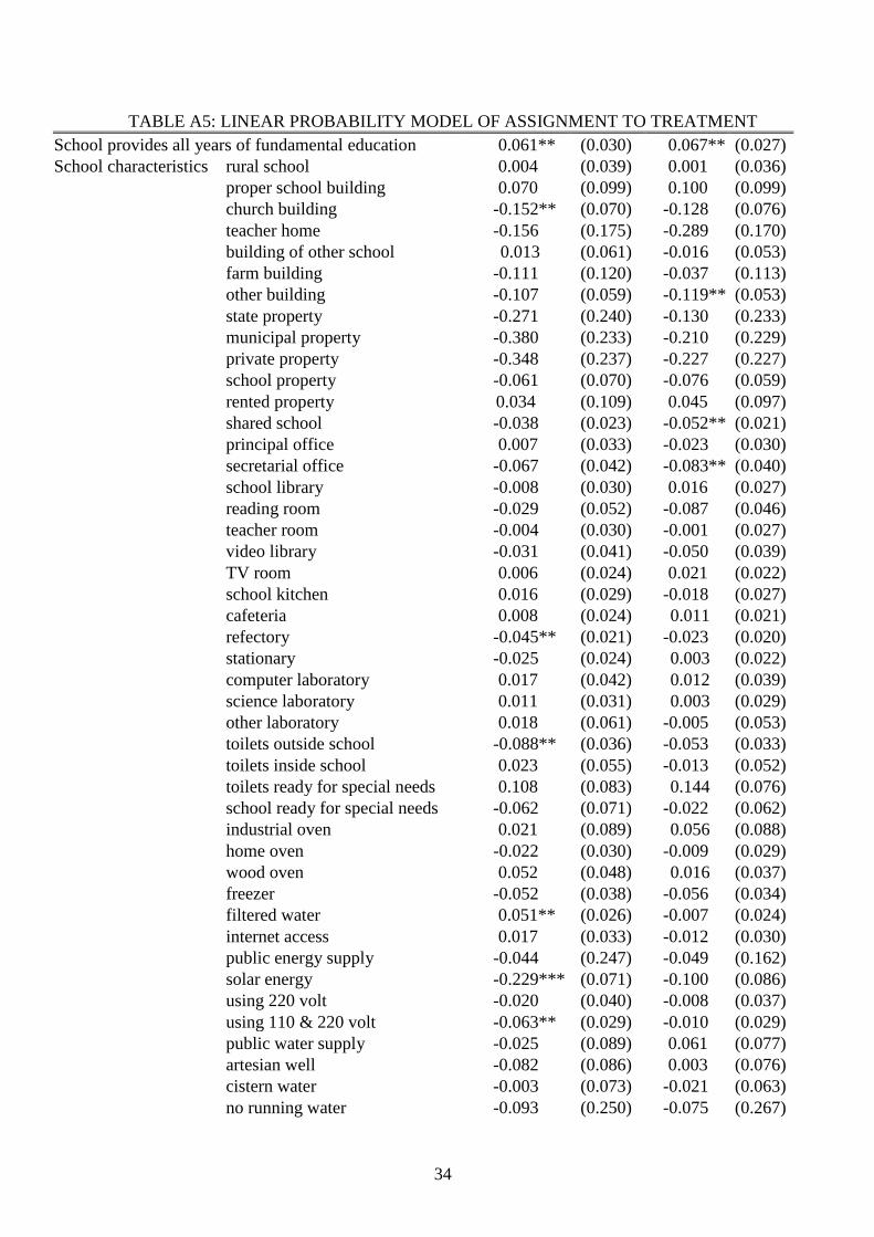
34

TABLE A5: LINEAR PROBABILITY MODEL OF ASSIGNMENT TO TREATMENT

School provides all years of fundamental education 0.061** (0.030) 0.067** (0.027)

School characteristics rural school 0.004 (0.039) 0.001 (0.036)

proper school building 0.070 (0.099) 0.100 (0.099)

church building -0.152** (0.070) -0.128 (0.076)

teacher home -0.156 (0.175) -0.289 (0.170)

building of other school 0.013 (0.061) -0.016 (0.053)

farm building -0.111 (0.120) -0.037 (0.113)

other building -0.107 (0.059) -0.119** (0.053)

state property -0.271 (0.240) -0.130 (0.233)

municipal property -0.380 (0.233) -0.210 (0.229)

private property -0.348 (0.237) -0.227 (0.227)

school property -0.061 (0.070) -0.076 (0.059)

rented property 0.034 (0.109) 0.045 (0.097)

shared school -0.038 (0.023) -0.052** (0.021)

principal office 0.007 (0.033) -0.023 (0.030)

secretarial office -0.067 (0.042) -0.083** (0.040)

school library -0.008 (0.030) 0.016 (0.027)

reading room -0.029 (0.052) -0.087 (0.046)

teacher room -0.004 (0.030) -0.001 (0.027)

video library -0.031 (0.041) -0.050 (0.039)

TV room 0.006 (0.024) 0.021 (0.022)

school kitchen 0.016 (0.029) -0.018 (0.027)

cafeteria 0.008 (0.024) 0.011 (0.021)

refectory -0.045** (0.021) -0.023 (0.020)

stationary -0.025 (0.024) 0.003 (0.022)

computer laboratory 0.017 (0.042) 0.012 (0.039)

science laboratory 0.011 (0.031) 0.003 (0.029)

other laboratory 0.018 (0.061) -0.005 (0.053)

toilets outside school -0.088** (0.036) -0.053 (0.033)

toilets inside school 0.023 (0.055) -0.013 (0.052)

toilets ready for special needs 0.108 (0.083) 0.144 (0.076)

school ready for special needs -0.062 (0.071) -0.022 (0.062)

industrial oven 0.021 (0.089) 0.056 (0.088)

home oven -0.022 (0.030) -0.009 (0.029)

wood oven 0.052 (0.048) 0.016 (0.037)

freezer -0.052 (0.038) -0.056 (0.034)

filtered water 0.051** (0.026) -0.007 (0.024)

internet access 0.017 (0.033) -0.012 (0.030)

public energy supply -0.044 (0.247) -0.049 (0.162)

solar energy -0.229*** (0.071) -0.100 (0.086)

using 220 volt -0.020 (0.040) -0.008 (0.037)

using 110 & 220 volt -0.063** (0.029) -0.010 (0.029)

public water supply -0.025 (0.089) 0.061 (0.077)

artesian well -0.082 (0.086) 0.003 (0.076)

cistern water -0.003 (0.073) -0.021 (0.063)

no running water -0.093 (0.250) -0.075 (0.267)

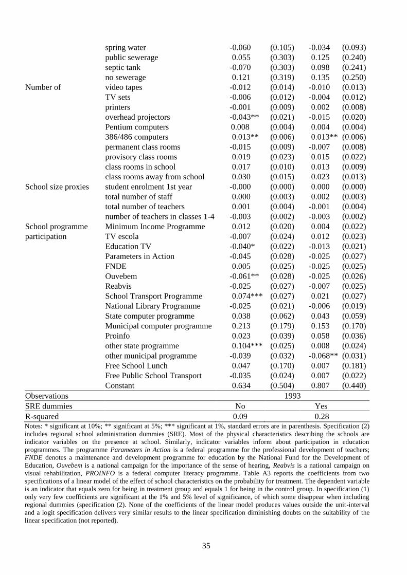
35

spring water -0.060 (0.105) -0.034 (0.093)

public sewerage 0.055 (0.303) 0.125 (0.240)

septic tank -0.070 (0.303) 0.098 (0.241)

no sewerage 0.121 (0.319) 0.135 (0.250)

Number of video tapes -0.012 (0.014) -0.010 (0.013)

TV sets -0.006 (0.012) -0.004 (0.012)

printers -0.001 (0.009) 0.002 (0.008)

overhead projectors -0.043** (0.021) -0.015 (0.020)

Pentium computers 0.008 (0.004) 0.004 (0.004)

386/486 computers 0.013** (0.006) 0.013** (0.006)

permanent class rooms -0.015 (0.009) -0.007 (0.008)

provisory class rooms 0.019 (0.023) 0.015 (0.022)

class rooms in school 0.017 (0.010) 0.013 (0.009)

class rooms away from school 0.030 (0.015) 0.023 (0.013)

School size proxies student enrolment 1st year -0.000 (0.000) 0.000 (0.000)

total number of staff 0.000 (0.003) 0.002 (0.003)

total number of teachers 0.001 (0.004) -0.001 (0.004)

number of teachers in classes 1-4 -0.003 (0.002) -0.003 (0.002)

School programme Minimum Income Programme 0.012 (0.020) 0.004 (0.022)

participation TV escola -0.007 (0.024) 0.012 (0.023)

Education TV -0.040* (0.022) -0.013 (0.021)

Parameters in Action -0.045 (0.028) -0.025 (0.027)

FNDE 0.005 (0.025) -0.025 (0.025)

Ouvebem -0.061** (0.028) -0.025 (0.026)

Reabvis -0.025 (0.027) -0.007 (0.025)

School Transport Programme 0.074*** (0.027) 0.021 (0.027)

National Library Programme -0.025 (0.021) -0.006 (0.019)

State computer programme 0.038 (0.062) 0.043 (0.059)

Municipal computer programme 0.213 (0.179) 0.153 (0.170)

Proinfo 0.023 (0.039) 0.058 (0.036)

other state programme 0.104*** (0.025) 0.008 (0.024)

other municipal programme -0.039 (0.032) -0.068** (0.031)

Free School Lunch 0.047 (0.170) 0.007 (0.181)

Free Public School Transport -0.035 (0.024) 0.007 (0.022)

Constant 0.634 (0.504) 0.807 (0.440)

Observations 1993

SRE dummies No Yes

R-squared 0.09 0.28 Notes: * significant at 10%; ** significant at 5%; *** significant at 1%, standard errors are in parenthesis. Specification (2)

includes regional school administration dummies (SRE). Most of the physical characteristics describing the schools are

indicator variables on the presence at school. Similarly, indicator variables inform about participation in education

programmes. The programme Parameters in Action is a federal programme for the professional development of teachers;

FNDE denotes a maintenance and development programme for education by the National Fund for the Development of

Education, Ouvebem is a national campaign for the importance of the sense of hearing, Reabvis is a national campaign on

visual rehabilitation, PROINFO is a federal computer literacy programme. Table A3 reports the coefficients from two

specifications of a linear model of the effect of school characteristics on the probability for treatment. The dependent variable

is an indicator that equals zero for being in treatment group and equals 1 for being in the control group. In specification (1)

only very few coefficients are significant at the 1% and 5% level of significance, of which some disappear when including

regional dummies (specification (2). None of the coefficients of the linear model produces values outside the unit-interval

and a logit specification delivers very similar results to the linear specification diminishing doubts on the suitability of the

linear specification (not reported).