Author's personal copy - Stanford...

This article appeared in a journal published by Elsevier. The attachedcopy is furnished to the author for internal non-commercial researchand education use, including for instruction at the authors institution

and sharing with colleagues.

Other uses, including reproduction and distribution, or selling orlicensing copies, or posting to personal, institutional or third party

websites are prohibited.

In most cases authors are permitted to post their version of thearticle (e.g. in Word or Tex form) to their personal website orinstitutional repository. Authors requiring further information

regarding Elsevier’s archiving and manuscript policies areencouraged to visit:

http://www.elsevier.com/copyright

http://www.elsevier.com/copyright

Author's personal copy

Large calculation of the flow over a hypersonic vehicle using a GPU

Erich Elsen *, Patrick LeGresley, Eric DarveDepartment of Mechanical Engineering, Stanford University, Durand Building 204, Stanford, CA 94305-4040, USA

a r t i c l e i n f o

Article history:Received 10 March 2008Received in revised form 29 July 2008Accepted 19 August 2008Available online 9 September 2008

Keywords:GPUBrookStream processingCompressible flowEuler equations

a b s t r a c t

Graphics processing units are capable of impressive computing performance up to518 Gflops peak performance. Various groups have been using these processors for generalpurpose computing; most efforts have focussed on demonstrating relatively basic calcula-tions, e.g. numerical linear algebra, or physical simulations for visualization purposes withlimited accuracy. This paper describes the simulation of a hypersonic vehicle configurationwith detailed geometry and accurate boundary conditions using the compressible Eulerequations. To the authors’ knowledge, this is the most sophisticated calculation of this kindin terms of complexity of the geometry, the physical model, the numerical methodsemployed, and the accuracy of the solution. The Navier–Stokes Stanford University Solver(NSSUS) was used for this purpose. NSSUS is a multi-block structured code with a provablystable and accurate numerical discretization which uses a vertex-based finite-differencemethod. A multi-grid scheme is used to accelerate the solution of the system. Based on acomparison of the Intel Core 2 Duo and NVIDIA 8800GTX, speed-ups of over 40� weredemonstrated for simple test geometries and 20� for complex geometries.

� 2008 Elsevier Inc. All rights reserved.

1. Introduction

In the last 5 years a new generation of processors, often called streaming processors, has become available for computeintensive applications. This new generation includes processors on graphics cards (GPU), ClearSpeed, Cell (IBM–Toshiba–Sony), and Merrimac (Stanford University). Special purpose processors like the GRAPE family have been available for a longertime. All these processors excel at arithmetic operations and boast performance in the range of 200–350 Gflops. As has beenrealized for some time now, increase in performance of processors becomes increasingly difficult to realize by simply shrink-ing the size of transistors and increasing the clock frequency. Furthermore, techniques that increase single core performancesuch as out-of-order execution, pipelining and branch prediction use large amounts of die space and consume significantamounts of power. Still, Moore’s law continues to apply: the number of transistors that can be placed on a chip is stillincreasing exponentially. Currently there are two different techniques to take advantage of all these transistors: CPUs putmore traditional cores on a die while GPUs have numerous smaller but less capable cores coupled with a very fast memorysystem. The NVIDIA 8800GTX for example has 128 scalar processors at 1.35 GHz capable of processing concurrently thou-sands of threads with a bandwidth to memory of 80 Gbytes/s.

In this paper, we focus on the use of GPUs for scientific codes. Several languages or programming environments have beendeveloped to utilize the computational power of GPUs: Sh (Michael McCool, University of Waterloo), Brook (Pat Hanrahan,Stanford University), CUDA (NVIDIA), CTM (AMD), and RapidMind. GPUs have already been used for many scientific appli-cations but there is still a significant gap between the reality of large scale engineering codes (hundreds of thousands of lines,days or weeks of computer time for a single simulation) and what has been accomplished using GPUs. Demonstrating a

0021-9991/$ - see front matter � 2008 Elsevier Inc. All rights reserved.doi:10.1016/j.jcp.2008.08.023

* Corresponding author.E-mail addresses: [email protected] (E. Elsen), [email protected] (P. LeGresley), [email protected] (E. Darve).

Journal of Computational Physics 227 (2008) 10148–10161

Contents lists available at ScienceDirect

Journal of Computational Physics

journal homepage: www.elsevier .com/locate / jcp


complex engineering application remains largely to be seen. In this paper, we present a real engineering flow calculationrunning on a single GPU with ‘‘engineering” accuracy and numerics. It demonstrates the potential of these processors forhigh performance scientific computing.

2. Review of prior work on GPUs

The current state of the art in applying GPUs to computational fluid mechanics is either simulations for graphics purposesemphasizing speed and appearance over accuracy, or simulations generally dealing with 2D geometries and using simplernumerics not suited for complex engineering flows. We now review some previous effort in this direction. The most notablework of engineering significance is the work of Brandvik [1] who solved an Euler flow in 3D geometry.

Krüger and Westermann [2] implemented basic linear operators (vector–vector arithmetic, matrix–vector multiplicationwith full and sparse matrices) and measured a speed-up around 12–15 on ATI 9800 compared to Pentium 4 2.8 GHz. Applica-tions to the conjugate gradient method and the Navier–Stokes equations in 2D are presented. Rumpf and Strzodka [3] appliedthe conjugate gradient method and Jacobi iterations to solve non-linear diffusion problems for image processing operations.

Bolz et al. [4] implemented sparse matrix solvers on GPU using the conjugate gradient method and a multi-grid acceler-ation. Their approach was tested on a 2D flow problem. A 2D unit square was chosen as test case. A speed-up by 2 was mea-sured with a GeForce FX.

Goodnight et al. [5] implemented the multi-grid method on GPUs for three applications: simulation of heat transfer, mod-eling of fluid mechanics, and tone mapping of high dynamic range images. For the fluid mechanics application, the vorticity–stream function formulation was applied to solve for the vorticity field of a 2D airfoil. This was implemented on NVIDIA Ge-ForceFX 5800 Ultra using Cg. A speed-up of 2.3 was measured compared to an AMD Athlon XP 1800.

In computer graphics where accuracy is not essential but speed is, flow simulations using the method of Stam [6] are verypopular. It is a semi-Lagrangian method and allows large time-steps to be applied in solving the Navier–Stokes equationswith excellent stability. Though the method is not accurate enough for engineering computation, it does capture the char-acteristics of fluid motion with nice visual appearance. Harris et al. [7] performed a rather comprehensive simulation ofcloud visualization based on Stam’s method [6]. Partial differential equations describe fluid motion, thermodynamic pro-cesses, buoyant forces, and water phase transitions. Liu et al. [8] performed various 3D flow calculations, e.g. flow over a city,using Stam’s method [6]. Their goal is to have a real-time solver along with visualization running on the GPU. A Jacobi solveris used with a fixed number of iterations in order to obtain a satisfactory visual effect.

The Lattice–Boltzmann model (LBM) is attractive for GPU processors since it is simple to implement on sequential andparallel machines, requires a significant computational cost (therefore benefits from faster processors) and is capable of sim-ulating flows around complex geometries. Li et al. [9,10] obtained a speed-up around 6 using Cg on an NVIDIA GeForce FX5900 Ultra (vs. Pentium 4 2.53 GHz). See the work of Fan et al. [11] using a GPU cluster.

Scheidegger et al. [12] ported the simplified marker and cell (SMAC) method [13] for time-dependent incompressibleflows. SMAC is a technique used primarily to model free surface flows. Scheidegger performed several 2D flow calculationsand obtained speed-ups on NV 35 and NV 40 varying from 7 to 21. The error of the results was in the range 10�2–10�3. Seealso the recent review by Owens et al. [14].

The work of Brandvik and Pullan [1] is the closest to our own. They implement a 2D and 3D compressible solver on theGPU in both BrookGPU and Nvidia’s CUDA. They achieve speed-ups of 29 (2D) and 16 (3D), respectively, although the 3DBrookGPU version achieved a speed-up of only 3. A finite volume discretization with vertex storage and a structured gridof quadrilaterals was used. No multi-grid or multiple blocks were used.

3. Flow solver

The Navier–Stokes Stanford University Solver (NSSUS) solves the three-dimensional Unsteady Reynolds Averaged Navier–Stokes (URANS) equations on multi-block meshes using a vertex-centered solution with first to sixth order finite differenceand artificial dissipation operators based on work by Mattson et al. [15], Svärd et al. [16], and Carpenter et al. [17] on Sum-mation by Parts (SBP) operators. Boundary conditions are implemented using penalty terms based on the SimultaneousApproximation Term (SAT) approach [17]. Geometric multi-grid with support for irregular coarsening of meshes is alsoimplemented. The prolongation and restriction operators are the standard full weighting except when irregular coarseningis required and for certain cells the prolongation becomes an injection and restriction is, naturally, the transpose of the pro-longation operator. The operators are applied to each block independently.

The SBT and SAT approaches allow for provably stable handling of the boundary conditions (both physical boundaries andboundaries between blocks). The numerics of the code are investigated in the work of Nordstorm et al. [18].

In this work, we focus on a subset of the capabilities in NSSUS, namely the steady solution of the compressible Euler equa-tions which come about if the viscous effects and heat transfer in the Navier–Stokes equations are neglected. Flows modeledusing the Euler equations are routinely used as part of the analysis and design of transonic and supersonic aircraft, missiles,hypersonic vehicles, and launch vehicles. Current GPUs are well suited to solving the Euler equations since the use of doubleprecision, needed for the fine mesh spacing required to properly resolve the boundary layer in RANS simulations, is notnecessary.

E. Elsen et al. / Journal of Computational Physics 227 (2008) 10148–10161 10149


The non-dimensional Euler equations in conservation form areoWotþ oE

oxþ oF

oyþ oG

oz¼ 0; ð1Þ

where W is the vector of conserved flow variables and E, F, and G are the Euler flux vectors defined as:

W ¼ ½q;qu;qv;qw;qe�;E ¼ ½qu;qu2 þ p;quv;quw;quh�;F ¼ ½qv;quv;qv2 þ p;qvw;qvh�;G ¼ ½qw;quw;qvw;qw2 þ p;qwh�:

In these equations, q is the density, u, v, and w are the cartesian velocity components, p is the static pressure, and h is thetotal enthalpy related to the total energy by h ¼ eþ p

q. For an ideal gas, the equation of state may be written as

p ¼ ðc� 1Þq e� 12ðu2 þ v2 þw2Þ

� �: ð2Þ

For the finite difference discretization a coordinate transformation from the physical coordinates (x,y,z) to the computationalcoordinates (n,g,f) is performed to yield:

oWotþ oE

onþ oF

ogþ oG

of¼ 0; ð3Þ

where W ¼W=J, J is the coordinate transformation Jacobian, and

E ¼ 1JðnxEþ nyFþ nzGÞ; F ¼ 1

JðgxEþ gyFþ gzGÞ; G ¼ 1

JðfxEþ fyFþ fzGÞ:

Discretizing the spatial operators results in a system of ordinary differential equations

ddt

Wijk

Jijk

!þ Rijk ¼ 0; ð4Þ

at every node in the mesh. An explicit five-stage Runge–Kutta scheme using modified coefficients for a maximum stabilityregion is used to advance the equations to a steady-state solution. The maximum stable timestep is computed based uponthe restriction of the fastest wave speed in the convection equations, i.e. the spectral radius.

Computing the residual R is the main computational cost; it includes the inviscid Euler fluxes, the artificial dissipation forstability, and the penalty terms for the boundary conditions. The penalty states, obtained either from physical boundary con-ditions or (for internal block boundaries) from the value of the flow solution in another block, are used to compute the pen-alty terms.

In the next sections, we describe our implementation of NSSUS for GPUs. This work was accomplished using BrookGPUwhich is a language that implements the streaming programming model on GPUs. We discuss the algorithms we created toimplement NSSUS on the GPU and report numerical results and performance measurements.

4. Brook

Brook (also known as BrookGPU) was designed by Ian Buck et al. [19–21]. Brook is a source to source compiler whichconverts Brook code into C++ code and a high-level shader language like Cg or HLSL. This code then gets compiled into pixelshader assembly by an appropriate shader compiler like Microsoft’s FXC or NVIDIA’s CGC. The graphics driver finally mapsthe pixel shader assembly code into hardware instructions as appropriate to the architecture. It can run on top of either Di-rectX or OpenGL; we used the DirectX backend for all results in this paper.

The syntax of Brook is quite simple. It is based on C with some extensions. The data is represented as streams which areessentially arrays. These streams are operated on by kernels which have specific restrictions: each kernel is a short programto be executed concurrently on each record of the output stream(s). This implies that each instance of a kernel automaticallyhas an output location associated with it. It is this location only to which output can be written. Scatter operations (writingto arbitrary memory locations) are not allowed. Gather operations (read with indirect addressing) are possible for inputstreams. Here is a trivial example:

kernel void add(float a[][], float b[][],out float resulthi) {float2 my_index=indexof(result).xy;result=a[my_index]+b[my_index];

}float ah100i; float bh100i; float ch100i;add(a,b,c);

10150 E. Elsen et al. / Journal of Computational Physics 227 (2008) 10148–10161


There will be one hundred of instances of the add kernel that are created, essentially implicitly executing a parallel forloop over all the elements of the output steam c. The indexof operator can be used to get the location a particular instance ofthe kernel will be writing to in the output stream(s).

5. Numerical accuracy considerations and performance comparisons between CPU and GPU

Producing identical results in a CPU and GPU implementation of an algorithm is, perhaps surprisingly, not a simple mat-ter. Even if the exact same sequence of instructions are executed on each processor, it is quite possible for the results to bedifferent. Current GPUs do not support the entire IEEE-754 standard. Some of the deviations are not, in the author’s experi-ence, generally a concern: not all rounding modes are supported; there is no support for denormalized numbers; and NaNand floating point exceptions are not handled identically. However, other differences are more significant and will affectmost applications: division and square root are implemented in a non-standard-compliant fashion, and multiplicationand addition can be combined by the compiler into a single instruction (FMAD) which has no counterpart on current CPUs.

X=A�B+C; // FMAD

This instruction truncates the result of the intermediate multiplication leading to different behavior than if the operationswere performed sequentially [22].

There are other differences between the architectures that can cause even a sequence of additions and multiplications(without FMADs) to yield different results. This is because the FPU registers are 80-bit on CPUs but only 32-bit on currentgeneration GPUs. If the following sequence of operations was performed:

C=1E5+1E-5; // C is in a register

D=10 � C; // C is still in a register, so is D

E=D - 1E6; // The result E is finally written to memory

On a GPU, E would be 0, while on a CPU it would contain the correct result of .0001. The result of the initial addition wouldbe truncated to 1E5 to fit in the 32-bit registers of a GPU unlike the CPU where the 80-bit registers can represent the result ofthe addition.

Evaluation of transcendental functions are also likely to produce different results, especially for large values of theoperand.

To further complicate matters, CPUs have an additional SIMD unit that is separate from the traditional FPU. This unit hasits own 128-bit registers that are used to store either 4 single precision or 2 double precision numbers. This has implicationsboth for speed-up and accuracy comparisons. Each number is now stored in its own 32-bit quarter of the register. The aboveoperations would yield the same result on both platforms if the CPU was using the SIMD unit for the computation.

In addition, by utilizing the SIMD unit, the CPU performs these four operations simultaneously which leads to a significantincrease in performance. Unfortunately, the SIMD unit can only be directly used by programming in assembly language orusing ‘‘intrinsics” in a language such as C/C++. Intrinsics are essentially assembly language instructions, but allow the com-piler to take care of instruction order optimization and register allocation. In most scientific applications writing at such alow level is impractical and rarely done; instead compilers that ‘‘auto-vectorize” code have been developed. They attempt totransform loops so that the above SIMD operations can be used.

6. Mapping the algorithms to the GPU

6.1. Classification of kernel types

In mapping the various algorithms to the GPU it is useful to classify kernels into four categories based on their memoryaccess patterns. All of the kernels that make up the entire PDE solver can be classified into one of these categories. Portions ofthe computation that are often referred to as a unit, the artificial dissipation for example, are often composed of a sequenceof many different kernels. For each kernel type we give a simple example of sequential C code, followed by how that codewould be transformed into streaming BrookGPU code.

The categories are:Pointwise. When all memory accesses, possibly from many different streams, are from the same location as the output

location of the fragment. A simple example of this type of kernel would be calculating momentum at all vertices by multi-plying the density and velocity at each vertex. Kernels of this type often have much greater computational density than thefollowing three types of kernels:

for (int i=0; i < 100; ++i)

c[i]=a[i]+b[i];

would be transformed into the above add kernel.



Stencil. Kernels of this type require data that is spatially local to the output location of the fragment. The data may or maynot be local in memory depending on how the 3D data is mapped to 2D space. Difference approximations and multi-gridtransfer operations lead to kernels of this type. These kernels often have a very low computational density, often performingonly one arithmetic operation per memory load.

for (int x=left; x < right; ++x)

for (int y=bottom; y < top; ++y)

res[x]=(func[x+1][y]+func[x-1][y]+func[x][y+1] +

func[x][y-1] - 4*func[x][y])/ delta;

would become

kernel void res(float delta, float func[][],out float reshi) {float2 my_index=indexof(res).xy;float2 up=my_index+float2(0, 1);float2 down=my_index - float2(0, 1);

float2 right=my_index+float2(1, 0);float2 left=my_index - float2(1, 0);

res=(func[up]+func[down]+func[right]+func[left] - 4*func[my_index])/delta;}

Unstructured gather. While connectivity inside a block is structured, the blocks themselves are connected in an unstruc-tured fashion. To access data from neighboring blocks, special data structures are created to be used by gather kernels whichconsolidate non-local information. Copying the sub-faces of a block into their own sub-face stream is a special case of thiskind of kernel.

kernel void unstructGather(float2 pos[][], float data[], out float reshufflehi) {float2 my_index=indexof(reshuffle);float2 gatherPos=pos[ my_index ];

reshuffle=data[ gatherPos ];

}

The contents of the pos stream are indices that are used to access elements of the data stream.Reduction. Reduction kernels are used to monitor the convergence of the solver. A reduction kernel outputs a single scalar

by performing a commutative operation on all the elements of the input stream. Examples include the sum, product or max-imum of all elements in a stream. Reduction operations are implemented in Brook using efficient tree data structures and anoptimal number of passes [19].

6.2. Data layout

Because the entire iterative loop of the solver is performed on the GPU, we do not need to be constrained by the datalayout the CPU version of NSSUS uses. A one-time translation to and from the GPU format can be done at the beginningand end of the complete solve with minimal overhead. This translation is on the order one second, whereas solves take min-utes to tens of minutes.

To lay the 3D data out in the 2D texture memory, we used the standard ‘‘flat” 3D texture approach [23] where each 2Dplane making up the 3D data is stored at a different location in the 2D stream. This leads to some additional indexing to fig-ure out a fragment’s 3D index from its location in the 2D stream (12 flops) and also additional work to convert back 3D indi-ces (9 flops). Data for each block in the multi-block topology is stored in separate streams; the solver loops over the blocksand processes each one sequentially.

6.3. Summary of GPU code

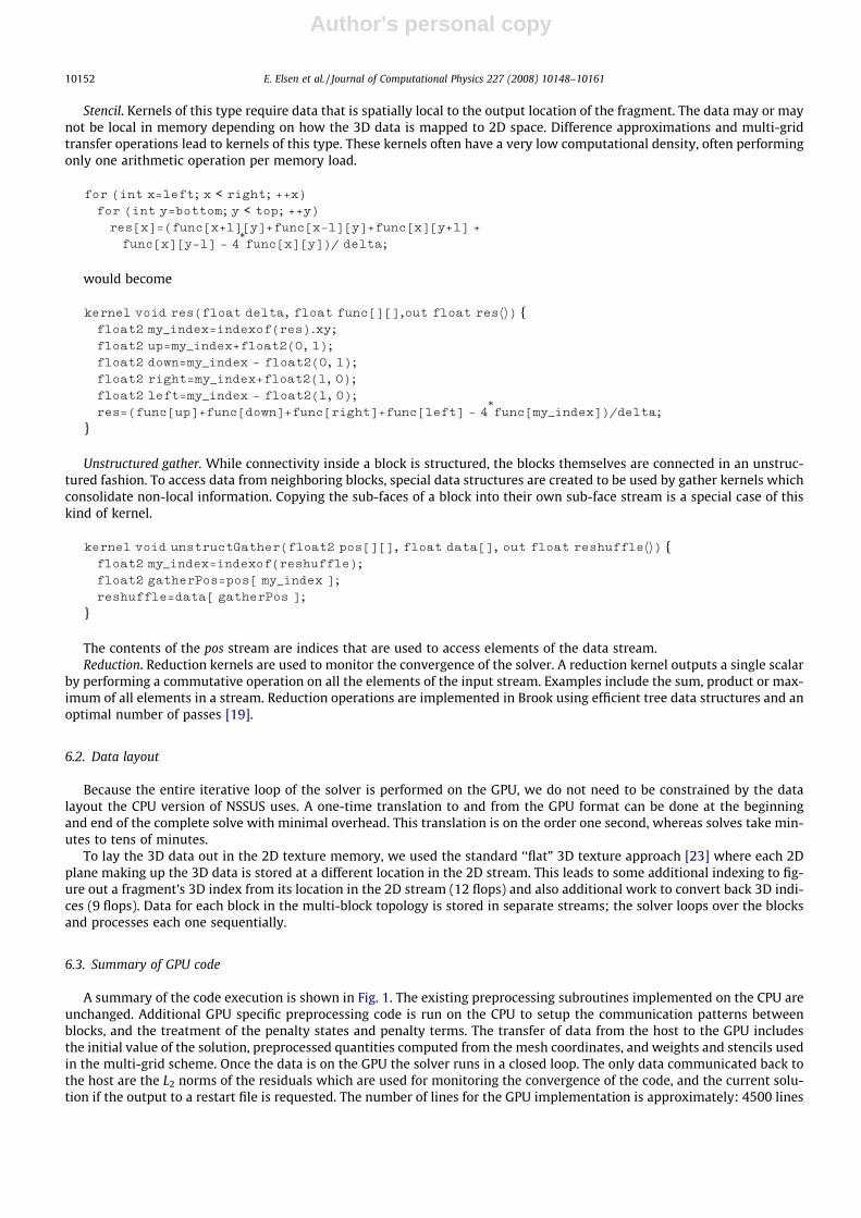
A summary of the code execution is shown in Fig. 1. The existing preprocessing subroutines implemented on the CPU areunchanged. Additional GPU specific preprocessing code is run on the CPU to setup the communication patterns betweenblocks, and the treatment of the penalty states and penalty terms. The transfer of data from the host to the GPU includesthe initial value of the solution, preprocessed quantities computed from the mesh coordinates, and weights and stencils usedin the multi-grid scheme. Once the data is on the GPU the solver runs in a closed loop. The only data communicated back tothe host are the L2 norms of the residuals which are used for monitoring the convergence of the code, and the current solu-tion if the output to a restart file is requested. The number of lines for the GPU implementation is approximately: 4500 lines



of Brook code, 8000 lines of supporting C++ code, and 1000 lines of new Fortran code. The original NSSUS code is in Fortran. Ittook the authors approximately 4 months to develop the necessary algorithms and make the changes to original code.

6.4. Algorithms

Constraints from the geometry of the mesh may require that in some blocks, especially at coarse multi-grid levels, thedifferencing in some directions is done at a lower order than otherwise desired if the number of points in that direction be-comes too small. To accommodate this constraint imposed by realistic geometries and also to avoid writing 27 different ker-nels for each possible combination of order and direction (up to third order is currently implemented on the GPU), we applyall differencing stencils in each direction separately.

The numerics of the code are such that one-sided difference approximations are used near the boundaries of the domain.We designate a boundary point as a point where a special stencil is needed, and interior point as a point where the normalstencil is applied (see Fig. 2). To illustrate the unique stencils created by the SBP approach and to have a concrete example forthe following discussion we describe the fourth order stencil:

dudx

��0¼ �24

17u0 þ

5934

u1 þ�4

17u2 �

334

u3;

dudx

��1¼ �1

2u0 þ

12

u2;

dudx

��2¼ 4

43u0 �

5986

u1 þ5986

u3 �4

43u4;

dudx

��3¼ 3

98u0 �

5998

u2 þ3249

u4 �4

49u5;

dudx

��i

¼ 112

ui�2 �8

12ui�1 þ

812

uiþ1 �1

12uiþ2:

This distinction presents a problem for parallel data processors such as GPUs because boundary points perform a differentcalculation from interior points and furthermore different boundary points perform different calculations. This can lead to

Inviscid fluxArtificial dissipationMultigrid forcing termsInviscid residualCopy sub-face dataBlock to block communicationPenalty state for physical boundary conditionsPenalty terms

Preprocessing

Preprocessing for GPU

Transfer data to GPU

Run solver on GPU

Return data from GPU

Write output file

while iteration < iterationsMax and solution not converged: loop over steps of the multigrid cycle:

if prolongation step: transfer correction/solution to fine grid if restriction step: transfer solution and residual to coarse grid if smoothing step:

compute residual compute time step store solution state update solution

compute residual loop over remaining Runge Kutta stages: update solution

compute residual update solution compute L2 norm of the residual

CPU GPU

Fig. 1. Flowchart of NSSUS running on the GPU.

Fig. 2. Node 0 is on the boundary. In a fourth-order scheme, nodes 0–3 would be considered boundary points.



terrible branch coherency problems, see Fig. 3. However, regardless of the order of the discretization, the branching can bereduced to only checking if the fragment is a boundary point or not. While the calculation for each boundary point is differ-ent, it can be computed as a dot product between stencil coefficients and field values. For example, the zeroth element of thecoefficient stream would consist of the values ð�24

17;5934;� 4

17;� 334Þ while another small position stream would hold the values

(0,1,2,3) describing the locations in u that correspond to the coefficients.Thus by using two small 1D streams (that can be indexed using the boundary point’s own location), only one branch to

determine if the point is a boundary point or in the interior instead of three for each possible stencil is required. (Note: wecount an if. . .else. . . statement as one branch.) The exact number depends on the branch granularity of the hardwarewhich is theoretically 4 � 4 on the 8800. However, GPUbench [24] suggests that in practice 8 � 8 performs better than4 � 4 and 16 � 16 even better than 8 � 8. For 16 � 16, the maximum possible number of branches is 15 but with this par-ticular stencil there are only nine possibilities – one interior point plus four right boundary points and four left boundarypoints (which can be adjacent due to the flat 3D layout). Our technique reduces this maximum to two, independent ofthe stencil – one branch for interior points plus one branch for right and left boundary points. Higher order differencingwould benefit even more from this technique.

Dealing with the boundary conditions and penalty terms in an efficient manner is significantly more difficult than eitherof the two previous cases. Fig. 4 shows how sub-faces and penalty terms are computed for each block. The unstructured con-nectivity between blocks leads to several sub-faces on each block. Each node on the blue block must be penalized against thecorresponding node on the adjacent blocks. For example, the node on the blue block located at the intersection of all fourgreen blocks must be penalized against the corner node in each of the four green blocks.

In Brook, it is not possible to stream over a subset of the entries in an array. Instead, we must go through all the O(n3)entries and use if statements to determine whether and what type of calculation need to be performed. This leads to a sig-

Fig. 3. This figure illustrates the stencil in the x-direction and the branching on the GPU. Each colored square represents a mesh node. The color correspondsto the stencil used for the node. Inner nodes (in grey) use the same stencil. For optimal efficiency, nodes inside a 4 � 4 square should branch coherently, i.e.use the same stencil (see square with a dashed line border). For this calculation, this is not the case near the boundary which leads to inefficiencies in theexecution. The algorithm we propose reduces branching and leads to only one branch (instead of 3 here).

Fig. 4. The continuity of the solution across mesh blocks is enforced by computing penalty terms using the SAT approach [17]. The fact that the connectivitybetween blocks is unstructured creates special difficulty. On this figure, for each node on the faces of the blue block, we must identify the face of one of thegreen blocks from which the penalty terms are to be computed. In this case, the left face of the blue block intersects the faces of four distinct green blocks.This leads to the creation of four sub-faces on the blue block. For each sub-face, penalty terms need to be computed. Note that some nodes may belong toseveral sub-faces. (For the interpretation of color in this figure legend the reader is referred to the web version of this article.)



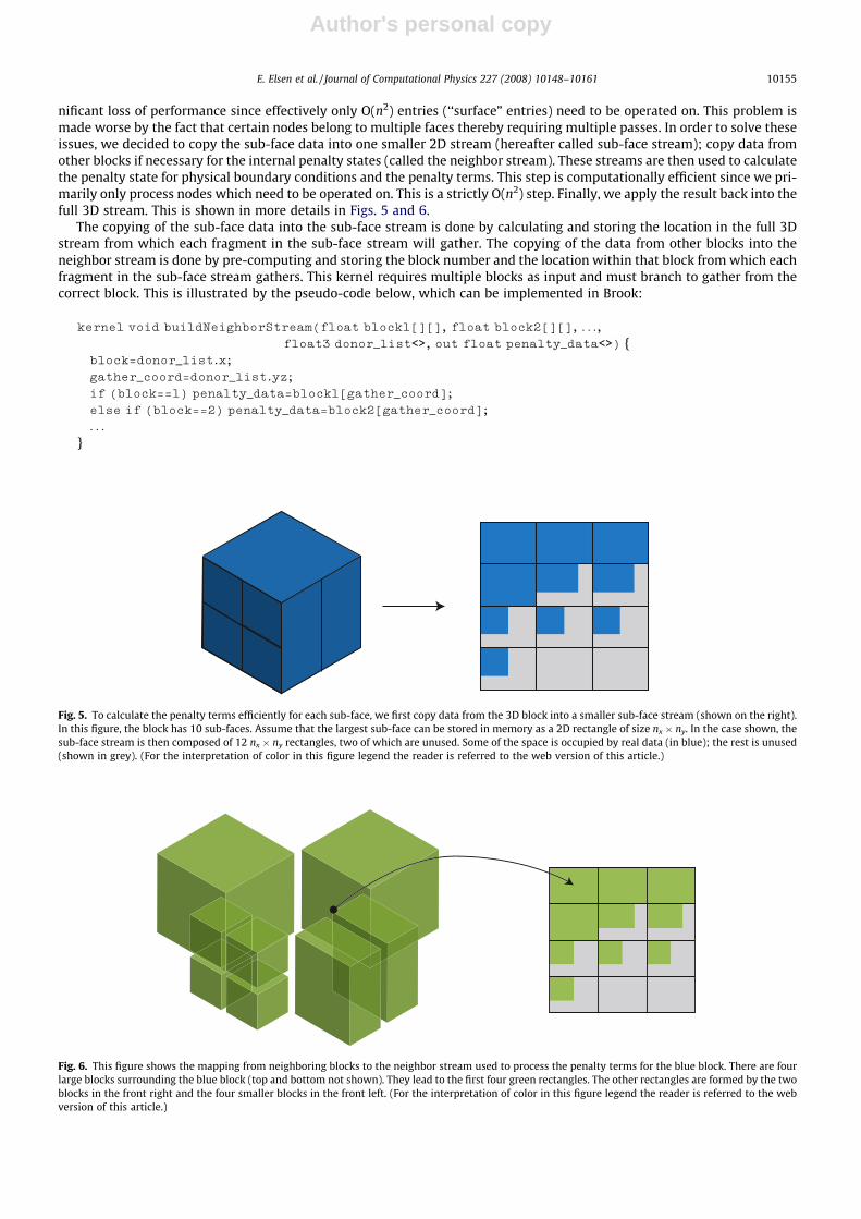
nificant loss of performance since effectively only O(n2) entries (‘‘surface” entries) need to be operated on. This problem ismade worse by the fact that certain nodes belong to multiple faces thereby requiring multiple passes. In order to solve theseissues, we decided to copy the sub-face data into one smaller 2D stream (hereafter called sub-face stream); copy data fromother blocks if necessary for the internal penalty states (called the neighbor stream). These streams are then used to calculatethe penalty state for physical boundary conditions and the penalty terms. This step is computationally efficient since we pri-marily only process nodes which need to be operated on. This is a strictly O(n2) step. Finally, we apply the result back into thefull 3D stream. This is shown in more details in Figs. 5 and 6.

The copying of the sub-face data into the sub-face stream is done by calculating and storing the location in the full 3Dstream from which each fragment in the sub-face stream will gather. The copying of the data from other blocks into theneighbor stream is done by pre-computing and storing the block number and the location within that block from which eachfragment in the sub-face stream gathers. This kernel requires multiple blocks as input and must branch to gather from thecorrect block. This is illustrated by the pseudo-code below, which can be implemented in Brook:

kernel void buildNeighborStream(float block1[][], float block2[][], . . .,

float3 donor_list<>, out float penalty_data<>) {block=donor_list.x;gather_coord=donor_list.yz;if (block==1) penalty_data=block1[gather_coord];else if (block==2) penalty_data=block2[gather_coord];. . .

}

Fig. 5. To calculate the penalty terms efficiently for each sub-face, we first copy data from the 3D block into a smaller sub-face stream (shown on the right).In this figure, the block has 10 sub-faces. Assume that the largest sub-face can be stored in memory as a 2D rectangle of size nx � ny. In the case shown, thesub-face stream is then composed of 12 nx � ny rectangles, two of which are unused. Some of the space is occupied by real data (in blue); the rest is unused(shown in grey). (For the interpretation of color in this figure legend the reader is referred to the web version of this article.)

Fig. 6. This figure shows the mapping from neighboring blocks to the neighbor stream used to process the penalty terms for the blue block. There are fourlarge blocks surrounding the blue block (top and bottom not shown). They lead to the first four green rectangles. The other rectangles are formed by the twoblocks in the front right and the four smaller blocks in the front left. (For the interpretation of color in this figure legend the reader is referred to the webversion of this article.)



An important point to make is that this method automatically handles the case of intersecting sub-faces (such as at edgesand corners) where multiple boundary conditions and penalty terms need to be applied. In that respect, this approach leadsto a significantly simpler code.

7. Results

The performance scaling of the code with block size is examined followed by an investigation of the performance of eachof the three main kinds of kernels. We, then, examine the performance on meshes for complex geometries typical of realisticengineering problems. In all our tests, the CPU used was a single core of an Intel Core 2 Duo E6600 (2.4 GHz, 4 MB L2 cache)and the GPU used was an NVIDIA 8800GTX (128 scalar processor cores at 1.35 GHz).

For all the results given below, we observed a consistent accuracy compared to the original single precision code in therange of 5–6 significant digits, including the converged solution for the hypersonic vehicle. This is the accuracy to be ex-pected since the GPU operates in single precision. We note that this good behavior is partly a result of considering the Eulerequation. The Navier–Stokes equations for example often require a very fine mesh near the boundary to resolve the bound-ary layer. In that case, differences in mesh element sizes may result in loss of accuracy.

7.1. Performance scaling with block size

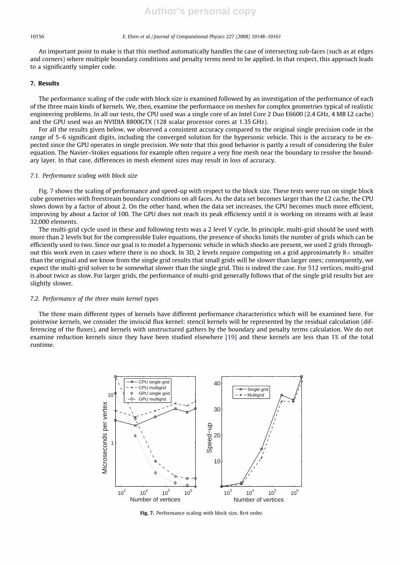
Fig. 7 shows the scaling of performance and speed-up with respect to the block size. These tests were run on single blockcube geometries with freestream boundary conditions on all faces. As the data set becomes larger than the L2 cache, the CPUslows down by a factor of about 2. On the other hand, when the data set increases, the GPU becomes much more efficient,improving by about a factor of 100. The GPU does not reach its peak efficiency until it is working on streams with at least32,000 elements.

The multi-grid cycle used in these and following tests was a 2 level V cycle. In principle, multi-grid should be used withmore than 2 levels but for the compressible Euler equations, the presence of shocks limits the number of grids which can beefficiently used to two. Since our goal is to model a hypersonic vehicle in which shocks are present, we used 2 grids through-out this work even in cases where there is no shock. In 3D, 2 levels require computing on a grid approximately 8� smallerthan the original and we know from the single grid results that small grids will be slower than larger ones; consequently, weexpect the multi-grid solver to be somewhat slower than the single grid. This is indeed the case. For 512 vertices, multi-gridis about twice as slow. For larger grids, the performance of multi-grid generally follows that of the single grid results but areslightly slower.

7.2. Performance of the three main kernel types

The three main different types of kernels have different performance characteristics which will be examined here. Forpointwise kernels, we consider the inviscid flux kernel; stencil kernels will be represented by the residual calculation (dif-ferencing of the fluxes), and kernels with unstructured gathers by the boundary and penalty terms calculation. We do notexamine reduction kernels since they have been studied elsewhere [19] and these kernels are less than 1% of the totalruntime.

103 104 105 106

1

10

Number of vertices

Mic

rose

cond

s pe

r ver

tex

103 104 105 106

10

20

30

40

Number of vertices

Spee

d−up

CPU single gridCPU multigridGPU single gridGPU multigrid

Single gridMultigrid

Fig. 7. Performance scaling with block size, first order.



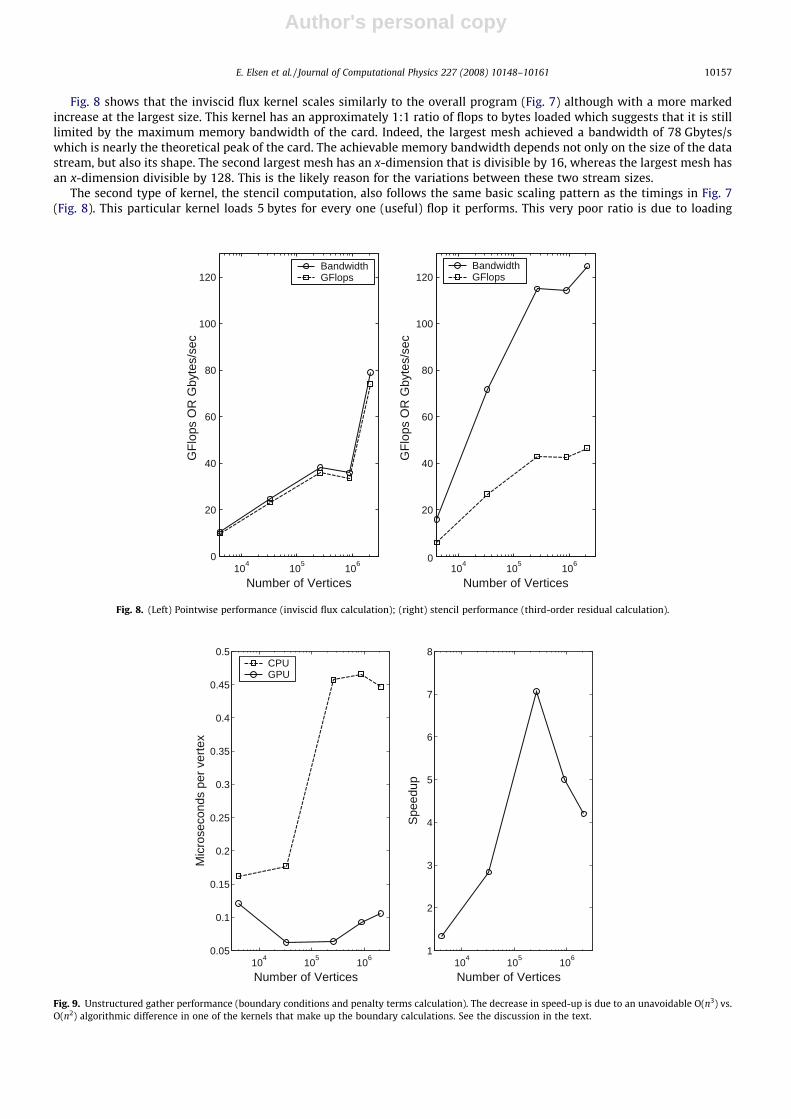
Fig. 8 shows that the inviscid flux kernel scales similarly to the overall program (Fig. 7) although with a more markedincrease at the largest size. This kernel has an approximately 1:1 ratio of flops to bytes loaded which suggests that it is stilllimited by the maximum memory bandwidth of the card. Indeed, the largest mesh achieved a bandwidth of 78 Gbytes/swhich is nearly the theoretical peak of the card. The achievable memory bandwidth depends not only on the size of the datastream, but also its shape. The second largest mesh has an x-dimension that is divisible by 16, whereas the largest mesh hasan x-dimension divisible by 128. This is the likely reason for the variations between these two stream sizes.

The second type of kernel, the stencil computation, also follows the same basic scaling pattern as the timings in Fig. 7(Fig. 8). This particular kernel loads 5 bytes for every one (useful) flop it performs. This very poor ratio is due to loading

104 105 1060

20

40

60

80

100

120

Number of Vertices

GFl

ops

OR

Gby

tes/

sec

BandwidthGFlops

104 105 1060

20

40

60

80

100

120

Number of Vertices

GFl

ops

OR

Gby

tes/

sec

BandwidthGFlops

Fig. 8. (Left) Pointwise performance (inviscid flux calculation); (right) stencil performance (third-order residual calculation).

104 105 1060.05

0.1

0.15

0.2

0.25

0.3

0.35

0.4

0.45

0.5

Number of Vertices

Mic

rose

cond

s pe

r ver

tex

CPUGPU

104 105 1061

2

3

4

5

6

7

8

Number of Vertices

Spee

dup

Fig. 9. Unstructured gather performance (boundary conditions and penalty terms calculation). The decrease in speed-up is due to an unavoidable O(n3) vs.O(n2) algorithmic difference in one of the kernels that make up the boundary calculations. See the discussion in the text.



the differencing coefficients as well as some values which are never used – a byproduct of the way some data is packed intofloat3s and float4s. Nonetheless, a very high bandwidth for this type of kernel is achieved. The bandwidth is in fact higherthan the memory bandwidth of card! This is possible because the 2D locality of the data access allows for the cache to beutilized very efficiently. The stencil coefficients, a total of 16 values, are also almost certainly kept in the cache.

The final type of kernel is the unstructured gather of which 3 out of the 5 kernels that make up the boundary and penaltyterm calculation consist. Its performance and scaling can be seen in Fig. 9. This routine does not see increased efficiency withlarger blocks and the speed-up vs. the CPU actually decreases after a point. To explain this, we examined each of the indi-vidual kernels. The first two are unstructured gather kernels that copy data to the sub-face streams and they run, as would beexpected, at approximately the random memory bandwidth of the card (�10 Gbytes/s). The next two are pointwise calcu-lations for the penalty terms which behave much like the inviscid flux kernel. The last kernel applies the calculated penaltiesto the volumetric data, which as mentioned above implies an implicit loop over the entire volume even though we only wishto apply the penalties to the boundaries. This is unavoidable because of the inability in Brook to scatter outputs to arbitrarymemory locations. Even though most of the fragments do little work other than determining if they are a boundary point ornot, as the block grows the ratio of interior to surface points increases and the overhead of all the interior points determining

X

Y

Z

Fig. 10. Three-block C-mesh around the NACA 0012 airfoil.

Fig. 11. Mach number around the NACA 0012 airfoil, M1 = 0.63, a = 2.



their location slows the overall computation down. In practice, however, it is unlikely that the size of a given block will belarger than 2 million elements; so in most practical situations, we are in the region where the GPU speed-up is large.

7.3. Performance on real meshes

The NACA 0012 airfoil (from the National Advisory Committee for Aeronautics) is a symmetric, 12% thick airfoil, that is astandard test case geometry for computational fluid dynamics codes. Fig. 10 shows the mesh with three blocks used for thissimulation (C-mesh topology) and Fig. 11 shows the Mach number around the airfoil.

The CPU code was compiled with the following options using the Intel Fortran compiler version 10: -O2 -tpp7 -axWP -ipo.

Table 1 shows the speed-ups for the NACA 0012 airfoil test case. As expected the speed-ups with multi-grid is lower thanwith a single grid because the computations on the coarser grids are not as efficient. However, over an order of magnitudereduction in computation time is still achieved.

For our final calculations, we used the hypersonic vehicle configuration from Marta and Alonso [25]. This is representativeof a typical mesh used in the external aerodynamic analysis of aerospace vehicles. It is a 15-block mesh; two versions wereused with approximately 720,000 and 1.5 million nodes. Because the blocks are processed sequentially on the GPU, animportant consideration is not only the overall mesh size but the sizes of individual blocks. For the 1.5 million node mesh,the approximate average block size is 100,000 nodes, with a minimum of 10,000 and a maximum of 200,000 nodes. Fig. 12shows the Mach number on the surface of the vehicle and the symmetry plane for a Mach 5 freestream.

In Table 2, we see the same general trend for speed-ups as the problem size and multi-grid cycle are varied. Beyond justthe pure speed-up, it is also important to note the practical impact of the shortened computational time. For example, a con-verged solution for the 1.5 M node mesh using a 2-grid multi-grid cycle requires approximately 4 CPU hours, but only about15 min on one GPU!

Table 1Measured speed-ups for the NACA 0012 airfoil computation

Order Multi-grid cycle Speed-up

First order Single grid 17.6Third order Single grid 15.1First order 2 Grids 15.6Third order 2 Grids 14.0

Note that higher orders and multiple grids generally lead to faster convergence, so that even though the speed-up is slightly reduced, the wall clock time toreach convergence would also be reduced (for both the CPU and GPU).

Fig. 12. Mach number – side and back views of the hypersonic vehicle.



8. Conclusion

We have implemented what we believe to be the most complex scientific simulation yet done on GPUs. Measured speed-ups range from 15� to over 40�. To demonstrate the capabilities of the code we simulated a hypersonic vehicle in cruise atMach 5 – something out of the reach of most previous fluid simulation works on GPUs. The three main types of kernels nec-essary for solving PDEs were presented and their performance characteristics analyzed. Suggestions to reduce branch inco-herency due to stencils that vary at the boundaries were made. We have also created a novel technique to handle thecomplications created by the boundary conditions and the unstructured multi-block nature of the mesh.

Our analysis has identified further ways in which the performance can be improved. Performance on small blocks islackluster and unfortunately with meshes around realistic geometries, small blocks often cannot be avoided. By groupingall the blocks into a single large texture, this problem could be avoided at the cost of increased indexing difficulties. Also,NVIDIA’s new language, CUDA, offers some interesting possibilities. It has an extremely fast memory shared by a group ofprocessors, the ‘‘parallel data cache”, which could be used to increase the memory bandwidth of the stencil calculations evenfurther. Scatter operations are also supported which means that the application of the penalty terms (at block interfaces)could scale with the number of surface vertices instead of the total number of vertices.

An important demonstration would be the use of a parallel computer with GPUs for fluid dynamics simulations. Thiswould establish the performance in a realistic engineering setting. It will impose some interesting difficulties because whilenodes will be on the order of 10� faster, the network speeds and latencies will not have changed and might be a bottleneck.

While the exact direction of future CPU developments is impossible to predict, it seems very likely that they will incor-porate many light computational cores very similar in nature to the fragment shaders of current GPUs. The techniques pre-sented here should thus be applicable to the general purpose processors of tomorrow.

Acknowledgments

This work has been supported by the US Department of Energy ASC program under contract No. LLNL B341491 as part ofthe Advanced Simulation and Computing Program (ASC). The authors wish to thank Edwin van der Weide for developing theCPU implementation of NSSUS and providing test cases for it, and San Gunawardana and Andre C. Marta for creating thehypersonic vehicle meshes.

References

[1] T. Brandvik, G. Pullan, Acceleration of a 3D Euler solver using commodity graphics hardware, in: 46th AIAA Aerospace Sciences Meeting and Exhibit,2008.

[2] J. Krüger, R. Westermann, Linear algebra operators for GPU implementation of numerical algorithms, in: ACM Trans. Graph. (Proceedings ofSIGGRAPH), 2003, pp. 908–916.

[3] M. Rumpf, R. Strzodka, Nonlinear diffusion in graphics hardware, in: Proceedings of EG/IEEE TCVG Symposium on Visualization VisSym ’01, 2001, pp.75–84.

[4] J. Bolz, I. Farmer, E. Grinspun, P. Schröder, Sparse matrix solvers on the GPU: conjugate gradients and multigrid, in: SIGGRAPH ’03: ACM SIGGRAPH2003 Papers, ACM, New York, NY, USA, 2003, pp. 917–924.

[5] N. Goodnight, C. Woolley, G. Lewin, D. Luebke, G. Humphreys, A multigrid solver for boundary value problems using programmable graphics hardware,in: HWWS ’03: Proceedings of the ACM SIGGRAPH/EUROGRAPHICS Conference on Graphics Hardware, Eurographics Association, Aire-la-Ville,Switzerland, 2003, pp. 102–111.

[6] J. Stam, Stable fluids, in: SIGGRAPH, 1999, pp. 121–128.[7] M.J. Harris, W.V. Baxter, T. Scheuermann, A. Lastra, Simulation of cloud dynamics on graphics hardware, in: HWWS ’03: Proceedings of the ACM

SIGGRAPH/EUROGRAPHICS Conference on Graphics Hardware, 2003, pp. 92–101.[8] Y. Liu, X. Liu, E. Wu, Real-time 3D fluid simulation on GPU with complex obstacles, in: 12th Pacific Conference on Computer Graphics and Applications,

6–8 October 2004, Seoul, South Korea, 2004, pp. 247–256.[9] W. Li, X. Wei, A. Kaufman, Implementing Lattice Boltzmann computation on graphics hardware, Visual Comput. 9 (2003) 444–456.

[10] W. Li, Z. Fan, X. Wei, A. Kaufman, GPU-based flow simulation with complex boundaries, GPU Gems 2, Addison-Wesley, 2005. pp. 747–764 (Chapter 47).[11] Z. Fan, F. Qiu, A. Kaufman, S. Yoakum-Stover, GPU cluster for high performance computing, in: SC ’04: Proceedings of the 2004 ACM/IEEE conference on

Supercomputing, IEEE Computer Society, Washington, DC, USA, 2004, p. 47.[12] C.E. Scheidegger, J.L.D. Comba, R.D. da Cunha, Practical CFD simulations on programmable graphics hardware using SMAC, Comput. Graph. Forum 24

(4) (2005) 715–728.[13] A.A. Amsden, F.H. Harlow, The SMAC method: a numerical technique for calculating incompressible flows, Tech. Rep. LA-4370, Los Alamos National

Laboratory, 1970.[14] J. Owens, D. Luebke, N. Govindaraju, M. Harris, J. Krüger, A.E. Lefohn, T.J. Purcell, A survey of general-purpose computation on graphics hardware,

Comput. Graph. Forum 26 (1) (2007) 80–113.

Table 2Speed-ups for the hypersonic vehicle computation

Mesh size Multi-grid cycle Speed-up

720 k Single grid 15.4720 k 2 Grids 11.21.5 M Single grid 20.21.5 M 2 Grids 15.8



[15] K. Mattson, M. Svärd, M. Carpenter, J. Nordström, Accuracy requirements for transient aerodynamics, in: 16th AIAA Computational Fluid DynamicsConference, Orlando, FL, 2003.

[16] M. Svärd, K. Mattsson, J. Nordström, Steady-state computations using summation-by-parts operators, J. Sci. Comput. 24 (1) (2005) 79–95.[17] M.H. Carpenter, D. Gottlieb, S. Abarbanel, Time-stable boundary conditions for finite-difference schemes solving hyperbolic systems: methodology and

application to high-order compact schemes, J. Comput. Phys. 111 (2) (1994) 220–236.[18] J. Nordstrom, E. van der Weide, J. Gong, M. Svard, A hybrid method for the unsteady compressible Navier–Stokes equations, Annual CTR Research

Briefs, Center for Turbulence Research, Stanford, 2007.[19] I. Buck, T. Foley, D. Horn, J. Sugerman, K. Fatahalian, M. Houston, P. Hanrahan, Brook for GPUs: stream computing on graphics hardware, ACM Trans.

Graph. 23 (3) (2004) 777–786.[20] I. Buck, High level languages for GPUs, in: SIGGRAPH ’05: ACM SIGGRAPH 2005 Courses, ACM, New York, NY, USA, 2005, p. 109.[21] D. Luebke, M. Harris, J. Krüger, T. Purcell, N. Govindaraju, I. Buck, C. Woolley, A. Lefohn, GPGPU: general purpose computation on graphics hardware, in:

SIGGRAPH ’04: ACM SIGGRAPH 2004 Course Notes, 2004, p. 33.[22] NVIDIA, CUDA Programming Guide 1.1, <http://developer.download.nvidia.com/compute/cuda/1_1/NVIDIA_CUDA_Programming_Guide_1.1.pdf>

November 2007.[23] A. Lefohn, GPU data structures, in: GPGPU: General-Purpose Computation on Graphics Hardware Tutorial, International Conference for High

Performance Computing, Networking, Storage and Analysis, November 2006.[24] I. Buck, K. Fatahalian, P. Hanrahan, Gpubench: evaluating GPU performance for numerical and scientific applications, in: Poster Session at GP2

Workshop on General Purpose Computing on Graphics Processors, 2004. URL <http://gpubench.sourceforge.net>.[25] A. Marta, J. Alonso, High-speed MHD flow control using adjoint-based sensitivities, AIAA paper 2006-8009, in: 14th AIAA/AHI International Space

Planes and Hypersonic Systems and Technologies Conference, Canberra, Australia, November 2006.


Author's personal copy - Stanford...

Documents

Transcript of Author's personal copy - Stanford...