Author's personal copy - SOEST | School of Ocean and …s personal copy ... School of Ocean and...

This article appeared in a journal published by Elsevier. The attachedcopy is furnished to the author for internal non-commercial researchand education use, including for instruction at the authors institution

and sharing with colleagues.

Other uses, including reproduction and distribution, or selling orlicensing copies, or posting to personal, institutional or third party

websites are prohibited.

In most cases authors are permitted to post their version of thearticle (e.g. in Word or Tex form) to their personal website orinstitutional repository. Authors requiring further information

regarding Elsevier’s archiving and manuscript policies areencouraged to visit:

http://www.elsevier.com/copyright

http://www.elsevier.com/copyright

Author's personal copy

Remote sensing of sand distribution patterns across an insular shelf: Oahu, Hawaii

C.L. Conger a,⁎, C.H. Fletcher b, E.H. Hochberg c, N. Frazer b, J.J.B. Rooney d

a University of Hawai'i at Manoa, School of Ocean and Earth Science, Sea Grant College Program, 2525 Correa Road, Honolulu, Hawai'i 96822, USAb University of Hawai'i at Manoa, School of Ocean and Earth Science, Department of Geology and Geophysics, 1680 East-West Road, Honolulu, Hawai'i 96822, USAc Nova Southeastern University, Oceanographic Center, 8000 North Ocean Drive, Dania Beach, FL 33004, USAd Joint Institute for Marine and Atmospheric Research, University of Hawaii, Pacific Islands Fisheries Science Center, National Marine Fisheries Service, Kewalo Research Facility,1125-B Ala Moana Blvd., Honolulu, HI 96814, USA

a b s t r a c ta r t i c l e i n f o

Article history:Received 16 April 2009Received in revised form 30 September 2009Accepted 6 October 2009Available online 17 October 2009

Communicated by J.T. Wells

Keywords:shelf sandreefspatial statisticsHawaiiremote sensingclassification

Sandy substrate is important as a resource, habitat, and dynamic region of the bathymetry. We find that sandstorage across the insular shelf of Oahu, Hawaii is controlled most strongly by general insular shelfmorphology and to a lesser degree by hydrodynamic energy. Shelf sand is predominantly found in waterdepths less than or crossing the 10 m contour. We use remote sensing to identify and classify 14,037individual sand deposits in nine study regions. A supervised classification algorithm aggregates these intofive classes with 14 subclasses. Almost 63% of all sandy surface area falls into two subclasses of the Channelsand Connected Fields class, 1) Major Channels and 2) Unchannelized Drainage. These subclasses connectregions of sediment production to regions of sediment storage on the insular shelf surface. This study is thefirst to quantitatively analyze and classify shelf sand deposits, in a high volcanic island coral reef setting.

© 2009 Elsevier B.V. All rights reserved.

1. Introduction

Sandy marine substrate is an important component of coastal andshelf habitat, a valuable resource for beach renourishment andconstruction, and a dynamic component of the bathymetry. Theshape and form of nearshore sand deposits have a pronounced effecton shoreline stability and constitute a significant portion of Hawaii'scoastal geologic framework (Fletcher et al., 2008). However, relativelylittle is known of shallow insular shelf sand bodies on low-latitudecoasts, despite the significance of nearshore sands in managing thecoastal environment (Bochicchio et al., 2009). This study aims tocharacterize meso-scale (10's of square meters to square kilometers)spatial patterns of sand occurrence on the shelf of Oahu, Hawaii (Fig. 1)with a generalized classification system based on spatial statistics.

In contrast to continental locations, where siliclastic sediment issupplied by streams and erosion of coastal sources, the sands of Oahuare primarily carbonate. They are composed of skeletal fragments ofmarine organisms and accumulate in relatively thin patches, fields,and linear deposits upon narrow insular shelf surrounding the island(Moberly et al., 1965; Harney et al., 2000; Harney and Fletcher, 2003;

Hampton et al., 2003; Grossman et al., 2006; Fletcher et al., 2008).Insular shelf sand bodies reflect a balance of factors includingproduction, temporary and permanent storage, and loss (includingabrasion, dissolution, bioerosion, and offshore transport; Harney andFletcher, 2003). A combination of hydrodynamic energy, waterquality, biologic productivity, and seafloor topography all controlcreation, destruction, and storage of carbonate sands. Historicalchanges in sea-level shape insular shelf morphology throughalternating subaerial and marine exposures, and combine withmodern coral communities to play key roles in shaping the storagecapacity of the insular shelf. Three studies (Moberly et al., 1975; SeaEngineering, 1993; Bochicchio et al., 2009) have cataloged thesenearshore sands.

Our study focuses on the sandy substrate extending from theshoreline to an approximate depth of 20 m below sea-level. Both coraland algal growth rates are highest in these depths (Stoddart, 1969)because of water circulation and nutrient availability, wave climate(Grigg and Epp, 1989; Grigg et al., 2002), and available light. Mostsediment on the insular shelf is produced by reef builders, reefdwellers, and reef bioeroders, making this zone the primary source ofnearshore sands. Only in the last 8500yr have sea-level rise andshoreline transgression led to the inundation of this portion of theinsular shelf (Grigg, 1998) and allowed for modern carbonateaccretion (Fletcher and Sherman, 1995; Harney et al., 2000; Grigget al., 2002; Harney and Fletcher, 2003, Grossman et al., 2006).

Marine Geology 267 (2009) 175–190

⁎ Corresponding author. Tel.: +1 808 587 0049; fax: +1 808 956 3259.E-mail addresses: [email protected] (C.L. Conger), [email protected]

(C.H. Fletcher), [email protected] (E.H. Hochberg), [email protected](N. Frazer), [email protected] (J.J.B. Rooney).

0025-3227/$ – see front matter © 2009 Elsevier B.V. All rights reserved.doi:10.1016/j.margeo.2009.10.005

Contents lists available at ScienceDirect

Marine Geology

j ourna l homepage: www.e lsev ie r.com/ locate /margeo


Fig. 1. Bathymetry and topography of Oahu coastal zone, interpolated from SHOALS LIDAR data and USGS DEM. A, B, C, and D showWaianae region; South of Laie Point and North ofLaie Point regions; Honolulu and Keehi Lagoon regions; and Lanikai, Kailua, Mokapu Point, and Kaneohe regions respectively.

176 C.L. Conger et al. / Marine Geology 267 (2009) 175–190


Most waves reach wave base within the zone 0–20 m and converttheir wave energy into shear stress across the sea floor, providing ameans for mechanical abrasion of both carbonate framework anddirect sediment producers (Storlazzi et al, 2003; Storlazzi et al, 2005).On Oahu, 20 m marks the approximate edge of the nearshore shelfthat terminates in a shallow, seaward facing scarp that is part of theKaneohe Shoreline Complex evident around much of the island(Stearns, 1974; Fletcher and Sherman, 1995). By extension of theHawaiian eolianite model proposed by Stearns (1970) and modifiedby Fletcher et al. (2005) where this scarp prevents sand transportupslope by winds during times of lowered sea-level, it may also act asa barrier for shoreward submarine transport except where channel-ized, similar to the fossil barrier reef off southeast Florida (Finkl,2004). Importantly, airborne and satellite sensors are capable ofaccurately imaging the sea floorwithin this depth range allowing us toprospect for sands via satellite imagery.

2. Regional setting

2.1. Insular shelf

Within the depth range of 0–20 m, morphology of the shelf aroundOahu results fromcarbonate accretion over recent interglacial cycles (fora review, see Fletcher et al., 2008). Most of the shelf in this depth zone isreefal in structure andMarine Isotope Stage (MIS) 7 in origin (Shermanet al., 1999). The front of the shelf is characterized by reefal carbonatesfrom MIS 5a–d, and the shallow landward portion in some areas iscovered by eolianites of similar age. Covering the shelf in a patchydistribution around the island and filling in available accommodationspace are Holocene reef carbonates (Grigg, 1998; Rooney et al., 2004;Grossman and Fletcher, 2004). The shelf surface has been sculptedthrough episodes of subaerialweathering and erosion characterizing thelast two interglacial cycles. Circumferential to Oahu, the shelf is almostentirely a fringing reef system with a shallow reef flat or a ramped reefface. Exceptions include Kaneohe Bay andpossibly Keehi Lagoon, both ofwhich are classified as lagoons with barrier reefs, or reefs intermediatebetween barrier and fringing morphologies (Guilcher, 1988).

2.2. Wave climate

Wave energy impacts accommodation space and mechanicalabrasion on the insular shelf and reef, as well as impacting coastlinestability and nearshore submarine sand transport. Bodge and Sullivan(1999) described four main components of Hawaii's regional waveclimate, as illustrated in Fig. 1. In the northwest Pacific, high-energywaves are created bywinter stormswith prolongedhighwinds directedat the northwestern shores of Hawaii. These waves are incident toshorelines facing from WNW to NNE with typical heights of 1.5–4.5 mand periods of 12–20 s, and extreme heights measured to 15 m. In thesouth Pacific, high winter (northern hemisphere summer) waves arecreated between April and October. These south Pacific waves typicallyhavedeep-water heights of 0.3–1.8 mandperiods of 12–20s. InfrequentKona storms produce moderately high-energy waves (around 9% of theyear) that approach from the south and west with heights of 3–4.5 mand periods of 6–10 s. Trade wind waves, the most consistent year-round wave type, have moderate energy and approach from thenortheast quadrant∼75%of theyear, for 90%of the summermonths and55–65% of the winter months (Grigg, 1998). Trade wind waves haveheights of 1.2–3 m and periods of 4–10 s. In addition to these four maintypes of waves, there are also the infrequent but highly destructivehurricane waves that impact nearshore reefs (Grigg, 1998).

3. Methods/materials

The first step in improving understanding of spatial distribution isanalyzing the two-dimensional meso-scale (10's of square meters to

square kilometers) surface characteristics of insular shelf sands.Spatial analysis is useful for identifying surface characteristicsassociated with insular shelf morphologies and is helpful for inferringorigin and history. The caveats for spatial analysis are that it fails toincorporate sand thickness, temporal variability, and sedimentcomposition properties.

3.1. Study regions

Nine Oahu study regions are defined using available QuickBirdSatellite© images. Study sites are chosen based on quality of availablescenes, diversity of the nearshore region, and representation ofdistinct types of shorelines. These are spread around the perimeter ofOahu, and cover approximately 39% of the total length of shorelineand 125 km2 of reef. The regions are detailed in Table 1.

3.2. Remotely sensed images

Four images were used in this study to characterize sedimentdistribution patterns in nearshore waters of Oahu. QuickBird Satellitescenes for this purpose were provided by DigitalGlobe, Inc., at http://www.digitalglobe.com. These are georectified, multi-channel (blue450–520 nm, green 520–600 nm, red 630–690 nm, and NIR 760–900 nm), TIFF images of Oahu, Hawaii, with 2.4 m pixel resolution.Images for regions are identified in Table 1.

3.3. LIDAR bathymetry

SHOALS (Scanning Hydrographic Operational Airborne LIDARSurvey) LIDAR (Light Detection and Ranging) was acquired andprocessed by the U.S. Army Corps of Engineers (USACE). LIDAR datafor regions is identified in Table 1. LIDAR coverage for the island ofOahu is both complete and dense, with an average nearest distancebetween points of ∼2.8 m. LIDAR points for each site (±5 cm verticalresolution) were interpolated using the Natural Neighbors techniquein ArcGIS, and rasterized to a pixel size of 2.4 m. Fig. 1 is a mosaic ofthe interpolated bathymetry, shaded for the depth range from 0 to35 m below mean sea-level for all study sites.

3.4. Image processing

Following the method in Conger et al. (2006), we decorrelatedboth blue and green bands from depth. This procedure coregistersbathymetry and satellite datasets, creating band pairs where eachpixel has a reflectance value and a known depth value. The deep-water reflectance of each band is subtracted from each pixel'sreflectance value. All subaerial regions, surface disturbances, highlyturbid waters, and LIDAR abnormalities are removed. An ln-transformof the reflectance data approximates the exponential attenuation oflight through the water column (Lyzenga, 1978). This simplifies therelationship between light attenuation and changes in water depth toa linear, highly correlated data distribution. Sample pixels are selectedacross the 0 to 20 m depth range from a single substrate type tominimize variance from reflector types (Mumby et al., 1998).Carbonate sands are used for this because of their easy identificationand presence at most depths. These sample pixels are used to modellight attenuation with depth. By relating the variability in each band'sintensity values to water depth a Principal Component Analysis (PCA)can be used to remove the correlation between depth and lightattenuation. A coordinate transformation is applied to an entire bandpair (Rencher, 2002). Output from this band pair rotation is a newcolor band where individual substrates no longer become darker asthe water column becomes deeper. Fig. 2A shows the rotated bluecolor band for a section of Kailua Bay reef used to develop and test thismethodology. Data and results from Isoun et al. (2003) were used forcomparison.

177C.L. Conger et al. / Marine Geology 267 (2009) 175–190


3.5. Substrate identification

Identification techniques include classification algorithms, banddensity slices, and analyst selection. The confounding effects of thewater column have made marine substrate classification based onreflectance, across large regions, marginally successful at best, with nosingle technique capable of routinely solving the problem. We use acombination of several techniques to reduce the effects of variation inwater columnproperties, atmospheric properties, and sea-surface state.

Simple classifier algorithms are used to segregate processedimages into two categories, Sand and Other Than Sand. A minimumdistance classifier (Rencher, 2002) is used on most image segments.Accuracy for classification runs is assessed by two methods: teststatistics (Rencher, 2002) and analyst interpretation. Test statisticsaccount for the number of correctly and incorrectly identified pixels,but are often insufficient for our purposes. We focus on analystinterpretation, which permits choosing the best classification based

on its spatial accuracy. Fig. 2B shows the classified image for a sectionof Kailua Bay.

In addition to the classification algorithms, application of a bandthreshold tool is used. The analyst can identify a specific intensitylevel in a single color band that separates carbonate sands (whichtend to be very bright) from all other, and darker, substrate types. Anadvantage of adjusting the intensity level, or threshold, for the Sand/Other Than Sand boundary is the accommodation of variable waterquality characteristics that otherwise introduce error. Increasedturbidity by non-carbonate suspended material usually darkens ascene, and carbonate sediment held in suspension usually brightens ascene. A combination of test statistics and analyst interpretation isused to verify successful identification.

Additionally, some sections of each scene are defined by the analystusing simple digitization. These locations are readily identifiable by ananalyst. For instance, steep slopes typically create marginal errors withimage processing. In these cases digitizing improves border definition

Table 1Study regions.

Region Shelf description Wave climate Coastal setting Remote sensing

Waianae b0.5 km–N1 km wide North Pacific swell Arid climate Digital GlobeRamped shelf face Kona storms Broad coastal plain 101001000173E702Numerous paleo-channels Hurricanes Modern beach USACE LIDAR

South Pacific swellNorth of Laie Point Narrow and shallow fringing shelf Trade wind waves Wet climate Digital Globe

Ramped shelf face North Pacific swell Narrow coastal plain 1010010002B85A01Eolianite islets Modern beach USACE LIDAR

South of Laie Point Wide and shallow fringing shelf Trade wind waves Wet climate Digital GlobeNumerous paleo-channels North Pacific swell Narrow coastal plain 1010010002B85A01

Modern beach USACE LIDARKaneohe Bay Shallow shelf Trade wind waves Seaward of the coastline Digital Globe

Ramped shelf face North Pacific swell Does not include lagoon or beaches 03MAR13205953Lagoon not included USACE LIDAR

Mokapu Peninsula Ramped shelf face Trade wind waves Coastal plain and post-erosional volcanics Digital GlobeVolcanic islet North Pacific swell Modern beach 03MAR13205953

USACE LIDARKailua Ramped shelf face Trade wind waves Wetland Digital Globe

Volcanic and carbonate islets North Pacific swell Beach ridge strand plain 03MAR13205953Paleo-channels Modern beach USGS LIDAR

Lanikai Wide and shallow fringing shelf Trade wind waves Beach ridge strand plain Digital GlobePaleo-channels North Pacific swell Modern beach 03MAR13205953

Basalt headlands USACE LIDARHonolulu Wide and moderately shallow fringing shelf Kona storms Coastal plain Digital Globe

Paleo and dredged channels Hurricanes Post-erosional volcano 1010010002D75F04South Pacific swell Filled wetlands USACE LIDAR

Keehi Lagoon Wide and shallow shelf Kona storms Seaward of lagoon Digital GlobePaleo and dredged channels Hurricanes Filled land and island 1010010002D75F04

South Pacific swell Modern beach USACE LIDAR

Fig. 2. A section of Kailua region is used as an example of the classification process. A mask, indicated by black pixels, is applied to the imagery. (A) Rotated blue color band,decorrelated from water depth. (B) Classified image, identifying sand (white) and everything other than sand (gray).



on adjacent sanddeposits. Some locationsdonot haveusable imagery orLIDAR data, but have been classified on the basis of field observations.The final result, from combined techniques, is a sand identificationimage of the entire study area, as seen in Fig. 3.

Normal image processing assumes both vertical and horizontalhomogeneity within the water column. As this is not usually the case,an image needs to be processed in several sections reflecting differentwater quality areas. Selection of the identification technique that isappropriate for each section is a function of water quality and variesacross each study region. Substrate identification methods are then

performed on each individual section. There may be regions in animage that are unusable, or must be identified by the analyst, as arethe cases where LIDAR data are not present or are incorrect, andwhere the imagery is obscured by clouds or sea-surface clutter. Thisprocess requires optically shallow waters, meaning that water mustbe sufficiently clear and shallow for the sensor to record an image ofthe bottom. This is important because the red and near infrared bandsprovide very little water penetration, and high turbidity can mask thebottom in the blue and green bands as well. Also, distinction betweenSand and Other Than Sand can be subjective, with the definition of

Fig. 3. All classified sands are displayed alongside a topographic map of Oahu. Sections A, B, C, and D correspond to the same sections in Fig. 1.



these two categories coming from within a continuum of substratevariation (as sand grades into hard substrate, rubble, algal meadows,etc.) being an analyst decision. This distinction and the subsequentselection of training classes define how and what we identify as sandysubstrate for our analysis. All supervised classification techniquesrequire analyst determinations in the beginning, by choosing trainingand test pixels from field data and image analysis. Our method allowsfor additional tuning by comparing the spatial qualities of the resultsto the image data, and by combining techniques to maximizeeffectiveness. These decisions are made according to the waterquality, bathymetry, substrate type, and results for each section.

3.6. Shape analysis

The classified image is segmented, using ENVI software, giving allof an individual sand deposit's pixels the same identification number.We identify a total of 14,037 sand deposits, with a minimum of fiveconnected pixels. We use Matlab to calculate a set of shapemeasurements for each sand deposit. We use six measurements,they are: area, orientation, eccentricity, form factor, roundness, andsolidity. Table 2 lists these measurements, their formulas, and a shortdescription of their physical meaning.

3.7. Image segregation

A supervised classification algorithm is used to identify fivediscrete classes of sand deposits. The five training classes aredescribed in Table 3. They are: 1. Channels and Connected Fields,2. Complex Fields and Very Large Depressions, 3. Large Depressions andFields, 4. Linear Deposits, and 5. Small Depressions and Simple Fields.

The five classes of sand deposits are split into three depth groups,providing insight into sand storage variability. These groups are: 0–10 m, 10–20 m, and those deposits that straddle the 10 m contour.The 10 m contour approximates the boundary of two insular shelfsub-environments: 1) shallow shelf limited by wave-generated shearforces where bathymetry largely reflects antecedent karst morphol-ogy, and 2) deeper shelf where wave forces are less significant and thebathymetry is more likely to reflect modern carbonate accretionrelated to reef growth. Also, shear stress from wave-generated andtidal currents determines sediment transport (Cacchione and Tate,1998; Storlazzi et al., 2004) across the insular shelf. Shear stressesfrom waves are a function of wave amplitude and water depth. The10 m contour is characterized by intermediate or transitional depthswhere the substrate is some combination of karst morphologymodified by modern reef growth. Comparing these depth groupshighlights the ability of the insular shelf to store sands in variablehydrodynamic conditions. Sand deposits within sub-environmentcrossing 10 m are of special interest as they contain the majority ofsurface area among sand deposits.

4. Results

The study area comprises nine regions, totaling approximately125 km2 of reef. Total surface area of identified sand deposits is about25 km2 or ∼20% of the total insular shelf area. Channels andConnected Fields account for the majority (64%) of all sand depositsurface area, and Complex Fields and Very Large Depressions accountfor 18%. Just over 72% of all sand deposit surface area straddles the10 m contour line, and 24% is b10 m. Combined sands crossing orshallower than 10 m represent more than 96% of all sand depositsurface area. When deposit classes are distinguished by depth range,Channels and Connected Fields that straddle the 10 m contouraccount for 63%, Complex Fields and Very Large Depressions b10 maccount for 10%, and Complex Fields and Very Large Depressions thatcross the 10 m contour account for 7%. Together, these threesubgroups total 80% of all surface area for sand deposits.

Study region boundaries are determined by physical variation asdescribed in Section 3.1, not size constraints. Total surface coverage ishighly dependent on the aerial extent of the region, so percentregional sand coverage, a normalized measure, is used to compareregions without the influence of aerial extent. Fig. 4 illustratesdifferences between total surface coverage and percent sand coverageby region. Regions containing the greatest absolute sand cover areKaneohe and South of Laie Point (Fig. 4A). However, percent regionalsand cover is greatest in Honolulu and Keehi Lagoon regions (Fig. 4B).

Fig. 5 displays a glyph plot for each region. Glyph plots are starshaped plots that assign spokes to each of five shape measurementsfor each region. The shape measure called orientation is not includedbecause in an island setting shorelines are oriented to all points on acompass. Longer spokes indicate a higher value relative to the other

Table 2Shape measurement equations and descriptions.

Area Pixelcount×(2.4 m)2

Converts pixel count to square meters

Orientation Relative tohistogram peakorientation

Each study region is adjusted so that ahistogram peak of all sand deposits is at zerodegrees, and all orientations are within ±90°,normalizing for all regions.

Form factor 4 × Area × πðPerimeterÞ2 Degree of rugosity around the perimeter of

each sand deposit, when compared to anequal area circle's perimeter.

Roundness 4 × Areaπ × ðMajor axisÞ2 Comparing sand deposit area to a circle with

radius equal to the deposit's major axis.Solidity Area

Convex area How full a sand deposit is, compared to asmooth shape whose perimeter intersects theouter points of the sand deposit's perimeter.

Eccentricityffiffiffiffiffiffiffiffiffiffiffiffiffiffiffiffiffiffiffiffiffiffiffiffiffiffiffiffiffiffiffi1− Minor axis2

Major axis2

� �rMeasures elongation of a sand deposit withinthe range from a circle (0) to a line (1).

Table 3Sand deposit class descriptions.

Classes Descriptions

Channels and ConnectedFields

Paleo-stream channels typically starting at or near theshoreline or a nearshore sand field and extending to anoffshore sand field. These are highly complex, veryelongate, non-rounded, open structures that cover largesurface areas.

Complex Fields and VeryLarge Depressions

Large sand fields made complex by their size, longperimeter, great number of outcrops, and ruggedinteraction with fringing substrate. Complex Fields andVery Large Depressions are significantly more roundedand solid than Channels and Connected Fields. Largegroups of interconnected depressions are also includedin this class.

Large Depressions andFields

Large openings in the insular shelf with steep sides, andfields smaller, less complex, and more solid thanComplex Fields and Very Large Depressions. Thesedepressions likely result from solution basins and blueholes filling with available sands. Though originaldepressions were formed as dolines, uvalas, andpossibly poljes during subaerial exposure, modernshape and orientation are likely due to coalescing andreshaping of depressions by modern hydrographicconditions. Medium sized fields also fit into this class.

Linear Deposits Sands in a linear and fairly simple shape. These fill inlinear depressions in the insular shelf, usually in spurand groove, ridge and runnel, or furrow morphologies.They are also elongate bands extended by current andwave energies across the insular shelf.

Small Depressions andSimple Fields

Depressions are individual dolines or small uvalas.Fields are very simple fields, often filling in minorswales or undulations on the insular shelf. Similar tothose in Large Depressions and Fields, except smallareas with much simpler shapes. The average size limitis around 140 m2, so they are only small by relativeterms.



regions. An example glyph is provided, with the measurementsrepresented by each spoke labeled. Percent regional sand coverage isused for area. Each glyph displays mean values for eccentricity,roundness, form factor, and solidity for each region. Two areas of theglyph are shaded in the example to illustrate one way to interpretthese plots. Complexity indicates a high degree of variability in theshape of the sand deposit. Elongation and circularity indicategeneralized geometries of sand deposits.

Dividing sand deposits into classes is an informational tool fordefining patterns within the data and mapping out variation betweenregions. Quantifying the validity for five classes is possible bycomputing User's accuracy (Rencher, 2002) from an error matrix(Table 4), by calculating the percent of objects identified as a certainclass that actually belong to that class. Accuracies are above 90% for allclasses except Channels and Connected Fields. The lower User'saccuracy results from identifying some deposits from other classes,

but this does not significantly change the accuracy of the total surfacearea classified. User's accuracy is most important because it quantifiesthe reliability of the classification results. High User's Accuracies implyhigh confidence in results.

Table 5 lists shape measurement means and standard deviationsfor each deposit class. Included in the table are bitmap imageexamples for each class, helpful in understanding actual sand depositsthat are associated with specific shapemeasurement statistics. Glyphscreated from the values listed, and short descriptions for each class areincluded to clarify differences. Also included are small images of sanddeposits in each of 14 subclasses. These subclasses are identified bygeologic analysis. Variability is represented by one standard deviationabout the mean value. Areas have large standard deviation becausethe surface areas for specific shapes can vary greatly. This does notmean that area measurements are inaccurate; rather they are highlyvariable within each class and have a wide range of values.

Fig. 4. Two bar plots: A) total sand area by region, and B) total percent sand coverage in each region, normalized by surface area for each region. Overlapping each region's bar is ashorter bar representing the surface coverage for the channels and connected fields crossing the 10 m contour, which accounts for a majority of sand deposit surface area.

Fig. 5. Glyph plots displaying mean sand deposit shape measurements for the nine regions with arms for percent regional area, eccentricity, roundness, form factor, and solidity.Example glyph is included.



Table 4User's and producer's accuracies for training classes.

Channels andConnected Fields

Complex Fields andVery Large Depressions

Large Depressionsand Fields

Linear Deposits Small Depressionsand Simple Fields

User's accuracy (%)

Channels and Connected Fields 15 3 3 0 0 71.43Complex Fields and Very Large Depressions 0 20 1 0 0 95.24Large Depressions and Fields 0 2 20 0 0 90.91Linear Deposits 0 0 0 25 0 100Small Depressions and Simple Fields 0 0 1 0 15 93.75Producer's accuracy (%) 100 80 80 100 100

Table 5



The total population is segregated into five sand deposit classes, initalics, each containing numerous individual sand deposits: Channelsand Connected Fields (97), Complex Fields and Very Large Depressions(103), Large Depressions and Fields (1282), Linear Deposits (1618), andSmall Depressions and Simple Fields (10,937).

Thefive sanddeposit classes are eachdefinedbyunique assemblagesof quantifiable shape measurements, as seen in Table 5. Within eachclass there are identifiable subclasses, defined using geologic analysis.Final sand deposit class structure is as follows:

1. Channels and Connected Fieldsa. Major Channelsb. Transitional Channelsc. Sand-Starved Channelsd. Unchannelized Drainagee. Misclassified Deposits

2. Complex Fields and Very Large Depressionsa. Fields with Steep Boundariesb. Reefal Strandlinesc. Radial Lineationsd. Very Large Depressionse. Open Fields

3. Large Depressions and Fieldsa. Large Depressionsb. Fields

4. Linear Deposits5. Small Depressions and Simple Fields

a. Small Depressionsb. Simple Fields

Channels and Connected Fields account for more than 64% of totalsand surface area while comprising less than 1% of individual sanddeposits. High mean eccentricity (0.945) and low mean roundness(0.128) combined with low mean values for both form factor (0.091)and solidity (0.422) depict elongate, narrow, moderately windingshapes with complex borders. The glyph for Channels and ConnectedFields highlights these distinctions. With respect to shape measure-ments, the glyph is almost opposite that of Small Depressions andSimple Fields. When considering the physical parameters of Channelsand Connected Fields, as large sediment conduits across the insularshelf, they contrast obviously with small, isolated deposits. Fig. 6shows all deposits in Channels and Connected Fields within the studyarea.

Five common subclasses of channels are identified: 1) MajorChannels, 2) Transitional Channels, 3) Sand-Starved Channels,4) Unchannelized Drainage, and 5) Misclassified Deposits. These areshown in Table 5.

Complex Fields and Very Large Depressions sand deposit classaccounts for 18% of the total sand surface area. Almost 17% of the totalsand coverage is from Complex Fields in Very Large Depressions inb10 m depth and crossing the 10 m contour, while barely 1% is found inN10 m depth. This does not, however account for all surface sands thatare stored in complex fields, as a large portion of nearshore and offshoresand fields are attached to sand channels and classified as Channels andConnected Fields. Moderate mean eccentricity (0.851) and roundness(0.269) describe shapes that are neither round or elongate. Very lowmean form factor (0.052) and below average mean solidity (0.422)implies a highly complex boundary to the shape. The glyph plot showssimilarity between Complex Fields and Very Large Depressions andLarge Depressions and Fields. Though similar, Complex Fields and VeryLarge Depressions is noticeably more elongate and complex, a result oflarger fields and more linked depressions creating complex individualsanddeposits. Orientations for this class are bimodalwith peaks that areboth shore-normal and shore-parallel.

There are, including those fields connected to channels, five mainsubclasses within Complex Fields and Very Large Depressions: 1) Fields

with Steep Boundaries, 2) Reefal Strandlines, 3) Radial Lineations,4) Very Large Depressions, and 5) Open Fields.

Several key features exist that distinguish this Large Depressionsand Fields from other sand deposit classes, including deposit size.Large Depressions and Fields contribute 10% of the total sand surfacearea. Overall deposit, simpler bathymetric lows, and many moresingle Large Depressions rather than collections of interconnecteddepressions, account for lower complexity values. Many of thesefeatures are more rounded or elliptical as well as less complex thanComplex Fields and Very Large Depressions, they tend to generatehigher solidity (0.549) and roundness (0.303) values, with lower formfactor (0.259) and eccentricity (0.785) values. This class (10% of totalsurface coverage) is predominately located in the 0–10 m depth (7% oftotal surface coverage).

Linear Deposits account for a very small percentage (under 2 %) ofthe overall sand surface area. They are located throughout the studyarea with over 75% in the 0–10 m depth. They are very elongate andsimple sand deposits. This class has eccentricity values (mean of0.975) almost equal to a line (1.00); and mean roundness (0.148),mean form factor (0.381), and mean solidity (0.686) values thatindicate simple, continuous features with smooth borders.

Small Depressions and Simple Fields account for the majority ofindividual sand deposits, with almost 78% of those identified in thisstudy, though they only contribute 6% of the total sand surface area.Shape measurements for this class are similar to Large Depressionsand Fields, though they reflect the simpler (mean form factor of1.017), rounder (mean roundness of 0.417 and mean eccentricity of0.821), and more solid (mean solidity of 0.834) characteristics ofthese smaller and more cleanly outlined deposits.

These sand deposits are ubiquitous across the depth controlled sub-environments, though most (68% of sand deposits and 75% of surfacecoverage for this class) are in the sub-environment b10 m depth. Only2% of these deposits are in the sub-environment crossing 10 m. Fewintersect the 10 m contour with radii averaging just less than 5 m. Thisclass is slightly more elongate than the larger depressions.

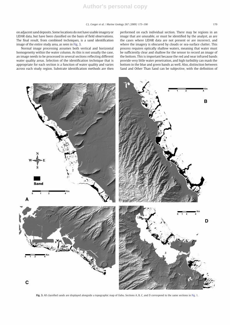
Fig. 7 contains bar plots of percent regional sand coverage for eachclass. The sum of all sand deposit classes is depicted in the All Regionsplot showing sand distribution pattern for the entire island-widestudy. Honolulu region's class distribution pattern is the closest to thatof the entire study area, while several regions (i.e. Lanikai, MokapuPoint, and North of Laie Point) have unique class distributions.

Honolulu region and Keehi Lagoon region have the highest percentregional sand coverage at 32% and 28% respectively.

5. Discussion

We analyze the occurrence of five sand deposit classes in the threesub-environments and the total study area of Oahu. Discussion beginswith a description of findings for the entire study area then narrows toa discussion of insular shelf environments.

5.1. Sand deposits

Total sand deposit population statistics for the 14,037 sand bodiesidentified are indicative of Oahu's sand distribution patterns and tosome degree its insular shelf morphology. Each of these is acontinuous sand body on the reef surface with a minimum size offive pixels, or 28.8 m2. Most are located in low-lying sections of thebathymetry, produced by subaerial exposure of the fossil reef andmodern reef growth. The degree of influence these two processesexert on insular shelf morphology is largely controlled by depth ofwater (including past sea-level lowerings) and wave climate.

5.1.1. Channels and Connected FieldsMajor Channels are easily identified through bathymetry or an

image of the insular shelf and are accurately identified by the



supervised classification. When filled with sand, these units almostalways connect to both nearshore and offshore sand fields, acting asconduits for sand movement in onshore and offshore directions.

Major Channels are likely the result of superimposed streams thatincised fossil reef during sea-level low-stands. In every case, channelaxes are aligned with or in close proximity to their respective moderndrainage systems in the adjoining watershed. These sand deposits aretypically shore-normal in orientation. Exceptions exist when severalstream channels feed into a single sand deposit. All sand deposits inthis class cross the 10 m contour.When combinedwith deposits in the

subclass Unchannelized Drainage (also in sub-environment crossing10 m), they account for almost 63% of total sand coverage and almostall of Channels and Connected Fields' sand coverage.

Two subclasses Transitional Channels and Sand-Starved Channelsboth lack connectivity between nearshore and offshore sand fields.Limited number of examples on the reef indicates that it is rare for achannel to be filled by modern growth (Purdy, 1974). Major Channelsdevelop from broad superimposed paleo-streams, as evidenced byGrossman and Fletcher (2004) who drilled the walls of a paleo-channel in Kailua Bay. They found that though reef growth is

Fig. 6. All Channels and Connected Fields class are displayed alongside a topographic map of Oahu. Sections A, B, C, and D correspond to the same sections in Figs. 1 and 3.



extensive on the walls, it was not sufficient to close the channel.However, immediately south is a much narrower Transitional Channelbeing closed by modern growth. In the 10–20 m depth, where growthgenerally dominates modern morphology, this channel is expressedas a series of separated depressions, all connected by a winding andnarrow depression in the insular shelf (paleo-channel). In the 0–10 mdepth, where antecedent topography controls bathymetry, thechannel is properly classified.

This example emphasizes that our classification system workswhere channels maintain original morphology. In the 10–20 m depthdeposit morphology is controlled more by reef growth into accom-modation space than the conduit's transportation of sand. The closeproximity of this Transitional Channel to a Major Channel, both ofwhich share common hydrodynamic and ecologic environments,implies that a combination of channel width and depth are needed topreserve both channel morphology and sand conduit capability.

Sand-Starved Channels are completely disrupted and no longeractive conduits of sand. Several examples of Sand-Starved Channelsare identified in the bathymetry. Sand-Starved Channels are blockedby lithified outcrops rather than modern growth. One example is aformer channel that is bisected by an eolianite outcrop dating fromMIS 5a–d (Fletcher et al., 2005). The outcrop bisects the channel and istherefore younger. Sand-Starved Channels contain limited patches ofsand and provide interesting examples of sand storage responsewhennearshore and offshore sand deposits are not connected. Thoughactive channels may have outcroppings of rock within channel walls,

the distinction of Sand-Starved Channels is that outcrops extendacross the width of the channel and are higher than channel walls.

Unchannelized Drainage is identified by analyzing local watershedand drainage patterns for evidence of small waterways related toflood drainage or wetlands during lower sea-levels. These are minordrainage systems that do not show modern evidence of permanentchannels through the subaerial, porous limestone. Modern bathym-etry resembles a group of interconnected, sand-filled depressionsextending from the shoreline down to the offshore fields. Thismorphology is likely the product of karst processes acting on thecarbonate bedrock of the coastal plain. Unchannelized Drainagedeposits have high surface areas and are also in the sub-environmentcrossing 10 m.

Misclassified Deposits are classified as Channels and ConnectedFields because they have large surface areas, complex shapes, and areelongate in nature. However, they do not fit the geologic definition forChannels and Connected Fields, and are considered an error class.Included in this subclassification are almost all the known, sand-filled,engineered (dredged) depressions. Engineered depressions wereidentified as Large Depressions and Fields for training the classifier,though their actual shapes are much closer to channels. Combined, allmisclassified shapes account for only a small portion (b1%) of theoverall sand deposit surface coverage. Unfortunately they have asignificant effect on User's accuracy for the classification algorithm.Minor effects on total sand storage are considered negligible, eventhough User's accuracy is lower.

Fig. 7. Bar plots showing class distributions for the five sand deposit classes as percent coverage in the entire study area and each of the nine study regions.



The connectivity between near- and offshore sands and the highsurface area of these deposits is important. They allow sands fromlower sea-levels to cross the 20 m scarp, supplying sediment to thenearshore sand budget. They store large volumes of sand, and they areproduction areas for modern sediment.

Sand production on Hawaii's insular shelves is associated withproductivity rates of organisms such as Foraminifera, mollusks,coralline (red) algae, Echinoids, corals, and Halimeda (Moberly et al.,1965). Moberly et al., found Foraminifera live in sand channels and onthe fore reef, but are not significantly present on the reef flat. Manyother sand components, with the exception of coralline algae, aretransported into the shallows from the reef edge.

Harney et al. (2000), during sediment research in Kailua Bay,found two primary sources of sediment. Offshore reef platforms areprimary sources for framework sediments (coral and coralline algae)while nearshore hardgrounds and landward portions of reef platformsare sources of direct sediment production (Halimeda, mollusks, andForaminifera).

Both Moberly et al. and Harney et al., agree that sedimentsproduced on the reef platform fill spaces there, move to shallowernearshore deposits, or move off the fore reef into deeper waters.Harney et al. found that sediment production on the nearshore reeffeeds sand deposits in the nearshore (including beaches) buteventually moves downslope toward offshore fields that are likelyto be terminal depositional sites. These researchers and Cacchione andTate (1998) indicate that sediments move both onshore and offshorewithinMajor Channels, acting as a conduit system between nearshoredeposits and offshore fields.

5.1.2. Complex Fields and Very Large DepressionsFields with Steep Boundaries are generally offshore sand fields

whose shoreward limits are either scarps on the insular shelf or steepsided morphologies like spur and groove. Low-energy and sedimentrich areas allow offshore fields to extend shoreward into thesegrooves. In the low-energy Honolulu region offshore Fields with SteepBoundaries, deeper spurs help to separate sand fields from channels,so they are identified as individual. Lower annual wave energy allowsfor greater abundance of sub-environments N10 m depth, withextensive spur and groove development extending across the insularshelf. This, combined with the occasionally present shallow terrace,provides increased storage space for sands. Honolulu has little netaccumulation of modern reef growth, as hurricanes wipe out mostmodern framework builders (Grigg, 1995). In addition, Waikikishoreline in Honolulu region has received multiple sand nourish-ments throughout the 20th and into the 21st century, of which∼150,000 m3 is no longer accountable on the beaches (Miller andFletcher, 2003). Assuming this volume has moved onto the insularshelf it is enough to cover all Honolulu region's sand deposits with∼5 cm of sand.

Reefal Strandlines (Blanchon and Jones, 1995) on the shallowfringing shelf are another significant subclass of Complex Fields andVery Large Depressions with linear features parallel to the direction ofwave approach across the insular shelf. Reefal Strandlines oftenextend straight back from the break in slope on the insular shelf tonear the shoreline. Near the landward end of channels the ReefalStrandlines curve toward the channel, indicating that nearshorecurrents strong enough to transport sediments are being focused intothe channels. Sediment production and storage along the ReefalStrandlines is linked to the beach system by wave transport and to theoffshore fields by the conduit behavior of the channels. Though thesefeatures may cover large surface areas, jet probing in Waikiki, Kailua,Lanikai, and Waimanalo (Bochicchio et al., 2009) suggests that theirthickness is usually minimal, indicating small volumes of sediment.Individual Reefal Strandlines often interconnect on the shallowfringing shelf, producing deposit orientations that are shore-parallel.

Radial Lineations (Guilcher, 1988) are oriented to wave approachacross the reef and are shaped by wave energy as sediment istransported toward the landwardmargin of the shallow fringing shelf.Radial Lineations are not thick deposits, but theymay adjoin sand caysand other types of sand accumulations. Three examples of RadialLineations were identified, all in lagoon environments.

Very Large Depressions are likely the result of karst features suchas dolines or uvalas developed during subaerial exposure of Oahureefal carbonates. Dolines form as roughly circular depressions up tothe size of valleys, while uvalas are typically more irregular in shapeand are larger in surface area. These are complex features in shallowwater with long-axes oriented in the direction of wave approach. It ismost likely that these depressions became linked after marineinundation.

The difference in geologic history between Very Large Depressionsand Fields with Steep Boundaries is from morphologic control due toantecedent topography rather than reef growth. This does not affectpotential sand storage space as both create relatively deep andinterconnected storage spaces for sands.

Open Fields appear to be located within minor depressions in thereef, and often contain many outcrops and irregular perimeters. Thissubclass fills in gentle bathymetric lows, or swales, and tapers out asthe basin floor rises to the surrounding hard bottom. Because of theshallow nature of these depressions, many outcrops extend throughthe sand deposit, and the borders are often very complex. Thissubclass is included in Complex Fields and Very Large Depressionsbecause of very high complexity values.

5.1.3. Large Depressions and FieldsFields, similar to Open Fields except that individual sand deposits

have less total surface area and are less complex, are less common. Theyalso account for far less total sand coverage than Large Depressions.

Many Large Depressions are single (or only a few connected) karstderived dolines. When located near the break in slope on the insularshelf, sand deposits in this class become more elongate and orientedin the direction of wave approach. Dolines developed in subaerialporous limestone show preferred orientations parallel tomajor trends(Ritter et al., 2002). Sub-environments in 0–10 m depth and crossingthe 10 m contour both show preferred orientation in a generallyshore-normal direction, while sub-environments in 10–20 m depthshow no preferred orientation. Though the Large Depressions werecreated by the same process of subaerial karstification, wave and tidalcurrent energies are needed to preserve and possibly accentuateoriginal depression shapes.

5.1.4. Linear DepositsThese sand deposits fill in linear depressions or are deposited in

linear sand ridges as a result of hydrodynamic conditions. Mostdeposits in the Linear Deposit class are oriented in the direction ofwave approach. Exceptions occur in two locations: sand depositslocated along the shoreline and large offshore sand deposits, both arecropped short by limits of detection within the imagery.

Percent regional sand coverage is fairly uniform for this class,though Keehi Lagoon and Mokapu Point regions have exceptionallyhigh and low percent coverage respectively. Keehi Lagoon's shallowshelf (0–10 m depth), high spur and groove coverage (10–20 mdepth), and extensive sand fields might explain the high number ofindividual sand deposits. High regional sand supply and limited waveenergy allow for filling of narrow and elongate reef morphologyfeatures. In higher energy systems these would either not be presentor would not hold sands, as elongate features may function ashydraulic pathways in the reef. The reason for Mokapu Point's lowcoverage (0.28%) is probably related to the lack of a shallow fringingshelf and its high wave energy. Linear Deposits sand class has thestrongest dependence on hydrodynamic conditions.



5.1.5. Small Depressions and Simple FieldsMorphologic features on the reef surface holding this class are very

similar to those holding Large Depressions.Most of these deposits are ineither Small Depressions filling in karst doline features or Simple Fields.

Those few sand deposits in the sub-environment crossing 10 mhave a much stronger shore-normal preferred orientation than theother two sub-environments. Doline features are being closed in thedeeper sub-environment, where reef growth controls availablesediment storage space on the seafloor. Simple Fields in the shallowersub-environments tend to includemany individual Reefal Strandlines,Radial Lineations, and bending or connected Linear Deposits. Thosewithin the sub-environment crossing 10 m give us a focused image ofsmall sand deposit response across the insular shelf on the 10 mcontour. Strong preferred orientation at this depth indicates controlby hydrodynamic conditions forcing a preferred orientation coinci-dent with limited reef growth.

An aspect of our methodology that may affect Small Depressionsand Simple Fields is that all processing is pixel-based, while allanalysis is shape-based. This transition affects marginally continuousbodies by identifying them as discrete and discontinuous sections. Aportion of this class is also the result of pixel resolution being toocoarse for imaging thin connections, resulting in a larger sand depositseparating into individual deposits. Even though these sand depositsare called “small,” theminimum size is five pixels or 28.8 m2, and theiraverage size is 138 m2, so they are large enough to be considered inenvironmental, ecologic, geologic, or resource studies.

5.2. Insular shelf types

A first order control in sand storage is provided by the generalmorphology of the insular shelf. Wide and shallow shelf areas with

well-defined breaks in slope have more surface area covered by sand,while deeper fringing shelf areas and lagoonal shelf faces have lesspercent sand coverage. A second order control is due to thehydrodynamic environment on similar reef geomorphologies. Sandstorage is highest in the general morphology we call low-energy wideshelf (Table 6) located on the south shore of Oahu. The followinginsular shelf types: medium-energy wide, seasonal high-energy deep,medium-energy deep, and high-energy deep, have decreasing sandstorage respectively (Table 6). The eastern shoreline of Oahu can bebroken into three categories, those receiving more north Pacific swell(Mokapu Point and North of Laie Point regions), those receiving lessnorth Pacific swell with wide shelves (Lanikai and South of LaiePoint), and those receiving less north Pacific swell with deep shelves(Kailua and Kaneohe Bay). The single region, Waianae, on the westernshoreline is a deep shelf. It has a high-energy environment in thewinter months as it receives direct and refracted north Pacific swell,but a low-energy environment in the summer months as it isprotected from trade wind waves. These insular shelf types andtheir sand deposits are illustrated in Fig. 8.

5.2.1. Low-energy wide shelfThe southern shoreline of Oahu, with a wide coastal plain, low-

energy environment, wide and shallow fringing shelf, shallow breakin slope, and extensive offshore sand fields is the model for high sandsurface coverage on Oahu. Honolulu and Keehi Lagoon regions,covering approximately 13% of Oahu's coastline, are both south-facingsections of insular shelf offshore of the Honolulu coastal plain. Thearea receiveswave energy primarily fromKona storm events, seasonalsouth Pacific swell, and occasional hurricanes. It is partially protectedfrom trade wind waves and is shadowed from winter swell.

Table 6Five general insular shelf types, regional environments, and sand storage characteristics.

General type: insular shelf Hydrodynamic energy environment Insular shelf geomorphology Keys and storage

Low-energy wide shelf South Pacific swell (summer) Shallow fringing shelf b0.5 km wide(wider before artificial alteration)

Major Channels0.3–1.8 m heights

b1–3 m deepUnchannelized Drainage

12–20 s periods Fields with Steep BoundariesKona storm waves (9% of year) Variable presence of distinct break in slope Open Fields3–4.5 m heights Reefal Strandlines6–10 s periods

0–3 m deepRadial LineationsMost abundant sand

Medium-energy wide shelf Trade wind waves (90% summer, 55–65% winter) Shallow fringing shelf N0.5 km wide Major Channels1.2–3 m heights b1–3 m deep Fields with Steep Boundaries4–10 s periods Open Fields

Refracted north Pacific swell (winter) Distinct shallow break in slope Reefal Strandlines1.5–4.5 m heights 1–3 m deep Large Depressions12–20 s periods 2nd most abundant sand

Seasonally high-energydeep shelf

Direct and refracted north Pacific swell (winter) Fringing shelf, variable width fromb0.5 km to N1 km wide, typically narrow

Major Channels1.5–4.5 m heights

2–10 m deepFields with Steep Boundaries

12–20 s periods Linear DepositsDirect and refracted south Pacific swell (summer)m heights Generally deep break in slope Small Depressions0.3–1.8 3–15 m deep12–20 s periods

3rd most abundant sand

Kona storm waves (9% of year)3–4.5 m heights6–10 s periods

Medium-energy deep shelf Trade wind waves (90% summer, 55–65% winter) Fringing shelf, variable width, generally N0.5 km Major Channels1.2–3 m heights 3–10 m deep Transitional Channels4–10 s periods Very Large Depressions

Refracted north Pacific swell (winter) Deep break in slope Large Depressions1.5–4.5 m heights N8 m deep 4th most abundant sand12–20 s periods

High-energy deep shelf Direct and refracted north Pacific swell (winter) Fringing shelf N0.5 km wide Major Channels1.5–4.5 m heights N3 m deep Sand-Starved Channels12–20 s periods Large Depressions

Trade wind waves (90% summer, 55–65% winter) Deep break in slope Small Depressions1.2–3 m heights N5 m deep Linear Deposits4–10 s periods Least abundant sand



High sand coverage may be the result of several factors. First, thisregion may have experienced increased sediment production acrossthe wide coastal plain during the Kapapa high stand. Harney et al.(2000) documented increased sediment production on a similarcoastal plain in Kailua, Oahu, during the higher sea-levels at that time.

Second, damage to the southern shoreline's reefs from the 1982 and1992 hurricanes was extensive, leaving piles of carbonate cobble andrubble where much of the living reef had formerly been (Grigg, 1995).Third, the area has been heavily dredged for channel creation andmaintenance, with much of the dredge spoil dumped on the insular

Fig. 8. Five general insular shelf types, a combination of morphology and hydrodynamic energy environment, that control sand coverage, class distribution, and sand deposit shapes.A) Low-energy wide shelf. B) Medium-energy wide shelf. C) Seasonally high-energy deep shelf. D) Medium-energy deep shelf. E) High-energy deep shelf.



shelf. Fourth, high non-point source nutrient influxes might lead toincreased production and consequent sediment volume increase inthe area.

Relatively lowwave energy fromSouthPacificwaves combinedwithinfrequent but catastrophic eventsmight help to explain the abundanceof carbonate sand along the southern shoreline. This does not explainthe disparity in surficial coverage between Honolulu and Keehi Lagoon.These two regions also show distinct differences in sand deposit classdistribution and overall sand deposit shape measurements, as seen inthe glyph plots. One possible factor is the addition of sediment in theHonolulu region during beach nourishment projects, as discussedearlier. Last, both Keehi Lagoon and Honolulu regions have artificiallyfilled coastline. The extensive loss of shallow shelf, an area of high sandcover, resulting from the development of airport runways and amanmade island has dramatically affected the Keehi Lagoon region.These three reasons are likely explanations for the disparity betweenpercent cover in Honolulu and Keehi Lagoon regions, where the generalconditions and hydrodynamic climate are otherwise very similar.

Mean sand deposit shape measurements, as seen in the regionalglyphs, show that mean values for Honolulu are distinct from all otherregions, and its distribution of surface coverage by classes is almostthe same as the entire study area's population. Keehi Lagoon on theother hand has a sand deposit class distribution similar to Kaneoheregion, the other lagoon environment, with high coverage in ComplexFields and Very Large Depressions and Linear Deposit classes andlower than average coverage in Channels and Connected Fields class.Keehi Lagoon region is similar to Lanikai in mean sand deposit shapemeasurements, as seen by their average glyphs, but this is probably aresult of loss of shallow shelf area from dredge and filling activities.Though these regions are in different energy environments, all havebroad and shallow shelves connected to well-defined and shallowbreaks in slope. Lanikai and South of Laie Point regions on the easternside of the island have similar morphologies but higher energyenvironments, are the next closest for percent sand coverage.

5.2.2. Medium-energy wide shelfLanikai and South of Laie Point regions have percent sand coverages

that are similar. Both have wide, shallow shelves and very shallow anddistinct breaks in slope. Mean sand deposit shape measurements, asseen in the regional glyphs, indicate that deposits in the Lanikai regionare closer in shape to the deposits found at Keehi Lagoon.

5.2.3. Seasonal high-energy deep shelfPercent sand coverage for the Waianae region is between those of

morphologies with wide and shallow shelves and those with narrowand deep shelves. Though the sand deposit class distribution andmorphology are similar to the Kailua region, the different energyenvironment allows for greater sand storage, as offshore sand fieldsextend into shallower depths. The offshore sand field is present in ourdepth of imaging around the offshoremouths of paleo-channels in theregion. These offshore sand fields are positioned next to ragged scarpsthat are the seaward edge of a sub-environment shallower than 10 m.

Sand deposits are primarily Channels and Connected Fields class,with seven major channel systems all connected to offshore sandfields. Undulations on the insular shelf provide space for sand storageas strong long-shore currents associated with north Pacific swellmove sediments along the coastline. An arid environment minimizesthe presence of overly large karst depressions. However, karstfeatures such as individual dolines or small uvalas are still presentwithin the region. Antecedent topography is well preserved in thisenvironment with the ragged scarp acting as the landward edge formost of the shallow offshore sand fields and is possibly inherited fromprevious sea-level transgressions during MIS 7and MIS 5. Aridconditions preserving several generations of karst features combinedwith a seasonally high-energy environment create a storage regime inWaianae that is a function of its antecedent topography. Offshore

fields account for the moderately high percent of seafloor covered bysand, even with the absence of a wide fringing shelf.

5.2.4. Medium-energy deep shelfKailua and Kaneohe have almost identical total percent sand

coverage and mean sand deposit shape measurements (glyphs). Bothhave prominent headlands to the north and south, both have similarpreferred sand deposit orientations, comparable moderate energyenvironments, large and active watersheds, very limited sand storagein the 10–20 m depth zone, and offshore sand fields deeper than thelimit of detection.

However, these two regionshave very differentmorphologies. Kailuais a deep fringing shelf showing evidence of widespread karstification,dominated by a single sandchannel andnearshore sandfield. Kaneohe isa lagoonal environment with a broad and shallow shelf and a rampedshelf face covered in linear morphologic features on several scales. It hasan active sand channel at each end, and multiple large sand fields alongthe landward margin. These differences are highlighted by sand depositclassdistributions. Kailua is similar to theWaianae region,witha rampedshelf face and a surface dominated by sand channels. Kaneohe, on theother hand, shares many characteristics with the Keehi Lagoon region.

5.2.5. High-energy deep shelfThe high-energy environments, Mokapu Point and North of Laie

Point, are both in front of wide coastal plains and have deep fringingshelves and minor sand fields that have been identified offshore. Boththese regions have low total percent sand coverage, and similar meansand deposit shape measurements (glyphs) and variations from theaverage for their sand deposit class distribution. Comparablemorphologies, high-energy environments, and the limited watersheddrainage for both of the regions explain these similarities. Higherenergy waves force the deepest sub-environment into waters beyondour depth of imaging. This preserves antecedent topography, allowingfor sand storage in depressions that would normally be filled orreshaped by reef growth. Lack of reef-controlled morphology reducesthe presence of hydrodynamically-controlled linear features in thisarea. Limited watershed drainage also reduces the presence of paleo-channels within regions. This results in a restricted conduit systemconnecting the shallower sub-environment extending deeper thanthe 10 m isobath, and dominated by antecedent topography, withoffshore sand fields deeper than the limit of detection.

6. Conclusions

First order control on sand storage is exerted by morphology, andsecond order control is provided by the level of hydrodynamic energywithin the environment. In addition, almost all surface sands are locatedin waters less than 10 m deep and in deposits that cross the 10 misobath. This is because the sub-environment shallower than 10mprecludes closure of depressions by modern reef growth, and conduitsystems between nearshore and offshore sand deposits act as storagebasins as well as conduits. These shallow areas also have the highestsediment production. The result is that the greatest sand storage is inboth shelves with offshore sand fields and some wide and shallowshelves, in low-energy environments (examples areHonolulu andKeehiLagoon). Second highest sand coverage is found on shelves withoutoffshore fields but with extensive wide and shallow shelves, andmoderately high wave energy (Lanikai, South of Laie Point). The thirdhighest coverage is in shelveswith offshorefields, butwithoutwide andshallow shelves, in seasonally high-energy environments (Waianae).Shelves without offshore fields and wide and shallow shelves have theleast sand coverage, though they can be further separated by the levelsofwave energy they are exposed to:moderately high (Kailua, Kaneohe),and high (Mokapu Point, North of Laie Point).

Percent regional sand coverage is highly indicative of generalmorphology and annual levels of wave energy. Sand deposit class



distribution and mean sand deposit shape measurements (glyphs)identify patterns associated with environmental factors. As anexample, the southern shoreline of Oahu is the most sand-rich reefon Oahu. Sediment productivity rates, a function of hydrodynamicclimate, ecology, and available sediment production space, are high.This is a result of exposure to refracted trade wind swell and SouthPacific swell. High-energy hurricane waves and anthropogenic effectsaid by providing short term, high volume increases to the sedimentbudget.

Sand deposit classification reveals that highest percent coverage iswithin the Channels and Connected Fields class. Major Channels andUnchannelized Drainage subclasses, both in the sub-environmentcrossing the 10 m isobath, account for almost all of this class' surfacecoverage. These two subclasses provide the connectivity betweennearshore and offshore sand fields, acting as conduits within the insularshelf's sediment system. They link nearshore zones of sedimentproduction with regions of sand storage.

The distinction of sand deposit classes is non-trivial. Class structuresneed significant numerical boundaries within shapemeasurements thatcorroborate well with physical boundaries within geologic settings.Because thedata is unimodal, use of a supervised classification algorithmis necessary and numerical boundary placement is an iterative process.Regardless, sand identification through remotely sensed data issignificantly faster and more accurate than hand digitizing. This processneeds strict analyst control, and some hand digitization is needed to filldata gaps.

Identification of sandy marine substrate is an important componentof any nearshore analysis targeting sediment resources, habitat, orsubstrate type. Additionally, these nearshore sands are a criticalcomponent of the littoral systems that control shoreline location onsandy coasts, as well as being highly mobile areas of the bathymetricprofiles. The process of identification and characterization of sandysubstrate is exportable to any coastal region, though the class structuredefined in this work is most applicable to high volcanic islands withinsular shelves. This process, if not the class structure itself, can be anintegral first step for studies researching critical marine habitats,sediment availability and transport, and coastal erosion.

Acknowledgments

We would like to acknowledge the Office of Naval Research forproviding the funding through award N00014-02-0799. We would alsolike to thank the U.S. Geological Survey and the U.S. Army Corps ofEngineers for providing the LIDAR data, and Digital Globe for providingtheQuickBirddata. C.L. Congerwishes to thankBillMorrison andAyeshaGenz for their continued support and technical expertise.

This paper is funded in part by a grant/cooperative agreement fromtheNational Oceanic andAtmospheric Administration, Project # R/TR-6,which is sponsored by the University of Hawaii Sea Grant CollegeProgram, SOEST, under the Institutional Grant No. NA05OAR4171048from theNOAAOffice of Sea Grant, Department of Commerce. The viewsexpressedherein are those of theauthor(s) anddonot necessarily reflecttheviewsofNOAAor anyof its subagencies. UNIHI-SEAGRANT-JC-10-01.

References

Blanchon, P., Jones, B., 1995. Marine-plantation terraces on the shelf around GrandCayman: a result of steppedHolocene sea-level rise. Journal of Coastal Research11 (1),1–33.

Bochicchio, C., Fletcher, C.H., Dyer, M., Smith, T., 2009. Reef-top sediment bodies:Windward Oahu, Hawaii. Pacific Science 63 (1), 61–82.

Bodge, K.R., Sullivan, S.P., 1999. Hawaii Pilot Beach Restoration Project: CoastalEngineering Investigation. State of Hawaii Department of Land andNatural Resources,Honolulu.

Cacchione, D.A. and Tate, G.B., 1998. Bottom currents, waves and sand transport in areef channel off Kailua, Hawai'i, First Regional Conference on Coastal ErosionManagement in Hawai'i and Other Pacific Islands, Kihei, Maui, Hawai'i.

Conger, C.L., Hochberg, E., Fletcher, C., Atkinson, M., 2006. Decorrelating remote sensingcolor bands from bathymetry in optically shallow waters. IEEE Transactions onGeoscience and Remote Sensing 44 (6), 1655–1660.

Finkl, C.W., 2004. Leaky valves in littoral sediment budgets: loss of nearshore sand to deepoffshore zones via chutes in barrier reef systems, southeast coast of Florida, USA.Journal of Coastal Research 20 (2), 605–611.

Fletcher, C.H., Sherman, C.E., 1995. Submerged shorelines on Oahu, Hawai'i: archive ofepisodic transgression during the deglaciation. Journal of Coastal Research,Holocene Cycles: Climate, Sea Levels, and Sedimentation 141–152 Special Issue 17.

Fletcher, C.H., et al., 2005. Age and origin of Late Quaternary eolianite, Kaiehu Point(Moomomi), Molokai, Hawaii. Journal of Coastal Research, Special Issue 54–73.

Fletcher, C.H., Bochicchio, C., Conger, C.L., Engels, M., Feirstein, E.J., Grossman, E.E.,Harney, J.N., Rooney, J.J., Sherman, C.E., Vitousek, S., Rubin, K., Murray-Wallace, C.V.(2008) Geology of Hawaii Reefs. Chapter 11 [54p] in “Coral Reefs of the U.S.A.”,Springer, 550p.

Grigg, R.W., 1995. Coral reefs in an urban embayment in Hawaii: a complex case historycontrolled by nature and anthropogenic stress. Coral Reefs 14 (4), 253–266.

Grigg, R.W., 1998. Holocene coral reef accretion in Hawaii: a function of wave exposureand sea level history. Coral Reefs 17, 263–272.

Grigg, R.W., Epp, D., 1989. Critical depth for the survival of coral islands: effects on theHawaiian Archipelago. Science 243 (4891), 638–641.

Grigg, R.W., et al., 2002. Drowned reefs and antecedent karst topography, AuauChannel, S.E. Hawaiian Islands. Coral Reefs 21, 73–82.

Grossman, E., Fletcher, C.H., 2004. Holocene reef development where wave energyreduces accommodation space, Kailua Bay, Windward Oahu, Hawaii, U.S.A. Journalof Sedimentary Research 74 (1), 49–63.

Grossman, E.E., Barnhardt, W.A., Hart, P., Richmond, B.M., Field, M.E., 2006. Shelfstratigraphy and influence of antecedent substrate on Holocene reef developmentsouth Oahu Hawaii. Marine Geology 226, 97–114.

Guilcher, A., 1988. Coral Reef Geomorphology. Coastal Morphology and Research. JohnWiley & Sons, New York.

Hampton, M.A., Blay, C.T., Murray, C., Torresan, L.Z., Frazee, C.Z., Richmond, B.M.,Fletcher, C.H., 2003. Data report geology of reef-front carbonate sediment depositsaround Oahu Hawaii. US Geological Survey Open-file Report 03-441.

Harney, J., Fletcher, C.H., 2003.A budget of carbonate framework and sedimentproduction,Kailua Bay, Oahu, Hawaii. Journal of Sedimentary Research 73 (6), 858–868.

Harney, J., Grossman, E., Richmond, B., Fletcher, C.H., 2000. Age and composition ofcarbonate shoreface sediments, Kailua Bay, Oahu, Hawaii. Coral Reefs 19, 141–154.

Isoun, E., Fletcher, C.H., Frazer, N., Gradie, J., 2003. Multi-spectral mapping of reefbathymetry and coral cover; Kailua Bay, Hawaii. Coral Reefs 22, 68–82.

Lyzenga, D., 1978. Passive remote sensing techniques for mapping water depth andbottom features. Applied Optics 17 (3), 379–383.

Miller, T.L., Fletcher, C., 2003. Waikiki: historical analysis of an engineered shoreline.Journal of Coastal Research 19 (4), 1026–1043.

Moberly, R., Baver, L.D., Morrison, A., 1965. Source and variation of Hawaiian littoralsand. Journal of Sedimentary Petrology 35 (3), 589–598.

Moberly, R., Campbell, J.F. and Coulbourn, W.T., 1975. Offshore and other sandresources for Oahu, Hawaii. UNIHI-SEAGRANT-TR-75-03, Sea Grant and the HawaiiInstitute of Geophysics, Honolulu.

Mumby, P.J., Green, E.P., Clark, C.D., Edwards, A.J., 1998. Digital analysis of multispectralairborne imagery of coral reefs. Coral Reefs 17 (1), 59–69.

Purdy, E.G., 1974. Reef configurations: cause and effect. In: Laporte, L.F. (Ed.), Reefs inTime and Space. Special Publication 18. Society of Economic Paleontologists andMineralogists, Tulsa, pp. 9–76.

Rencher, A., 2002. Methods of Multivariate Analysis. John Wiley & Sons, Inc., New York.708 pp.

Ritter, D.F., Kochel, R.C., Miller, J.R., 2002. Process Geomorphology. McGraw Hill, SanFrancisco. 560 pp.

Rooney, J., Fletcher, C.H., Grossman, E., Engels, M., Field, M., 2004. El Nino influence onHolocene reef accretion in Hawaii. Pacific Science 58 (2), 305–324.

Sea Engineering, I., 1993. Beach Nourishment Viability Study. Sea Engineering, Inc.,Waimanalo.

Sherman, C.E., Fletcher, C.H., Rubin, K.H., 1999. Marine and meteoric diagenesis ofPleistocene carbonates from a nearshore submarine terrace, Oahu, Hawaii. Journalof Sedimentary Research 69 (5), 1083–1097.

Stearns, H.T., 1970. Ages of Dunes on Oahu, Hawaii. Occasional Paper of Bernice P.Bishop Museum, 24(4): 50-72.

Stearns, H.T., 1974. Submerged shorelines and shelves in the Hawaiian Islands and arevision of some of the eustatic emerged shorelines. Geological Society of AmericaBulletin 85, 795–804.

Stoddart, D.R., 1969. Ecology and morphology of recent coral reefs. Biological Reviews44, 433–498.

Storlazzi, C.D., Logan, J.B., Field, M.E., 2003. Quantitative morphology of a fringing reeftract from high-resolution laser bathymetry: Southern Molokai, Hawaii. GeologicSociety of America Bulletin 115 (11), 1344–1355.

Storlazzi, C.D., Ogsten, A.S., Bothner, M.H., Field, M., Presto, M.K., 2004. Wave- andtidally-driven flow and sediment flux across a fringing coral reef: SouthernMolokai, Hawaii. Continental Shelf Research 24, 1397–1419.

Storlazzi, C.D., Brown, E., Field, M., Rogers, K., Jokiel, P.L., 2005. Amodel for wave controlon coral breakage and species distribution in the Hawaiian Islands. Coral Reefs 24,43–55.


Author's personal copy - SOEST | School of Ocean and …s personal copy ... School of Ocean and...

Documents

Transcript of Author's personal copy - SOEST | School of Ocean and …s personal copy ... School of Ocean and...