COWLES FOUNDATION DISCUSSION PAPER NO.

COWLES FOUNDATION FOR RESEARCH IN ECONOMICSYALE UNIVERSITY

Box 208281New Haven, Connecticut 06520-8281

http://cowles.yale.edu/

ATTRIBUTE SENTIMENT SCORING WITH ONLINE TEXT REVIEWS : ACCOUNTING FOR LANGUAGE STRUCTURE AND ATTRIBUTE SELF-SELECTION

By

Ishita Chakraborty, Minkyung Kim, and K. Sudhir

May 2019

2176

Attribute Sentiment Scoring with Online Text Reviews:

Accounting for Language Structure and Attribute Self-Selection

Ishita Chakraborty, Minkyung Kim, K. Sudhir

Yale School of Management

March 2019

We thank the participants in the marketing seminars at Kellogg, Penn State, UBC, the Yale SOM Lunch,

the 2018 CMU-Temple Conference on Big Data and Machine Learning, the 2019 Management Science

Workshop at University of Chile and the 2019 IMRC Conference in Houston.

1

Attribute Sentiment Scoring with Online Text Reviews:

Accounting for Language Structure and Attribute Self-Selection

The authors address two novel and significant challenges in using online text reviews to obtain

attribute level ratings. First, they introduce the problem of inferring attribute level sentiment from

text data to the marketing literature and develop a deep learning model to address it. While ex-

tant bag of words based topic models are fairly good at attribute discovery based on frequency

of word or phrase occurrences, associating sentiments to attributes requires exploiting the spatial

and sequential structure of language. Second, they illustrate how to correct for attribute self-

selection—reviewers choose the subset of attributes to write about—in metrics of attribute level

restaurant performance. Using Yelp.com reviews for empirical illustration, they find that a hy-

brid deep learning (CNN-LSTM) model, where CNN and LSTM exploit the spatial and sequential

structure of language respectively provide the best performance in accuracy, training speed and

training data size requirements. The model does particularly well on the “hard” sentiment classi-

fication problems. Further, accounting for attribute self-selection significantly impacts sentiment

scores, especially on attributes that are frequently missing.

Keywords: text mining, natural language processing (NLP), convolutional neural networks (CNN),

long-short term memory (LSTM) Networks, deep learning, lexicons, endogeneity, self-selection,

online reviews, online ratings, customer satisfaction

2

INTRODUCTION

Crowd-sourced online review platforms such as Yelp, TripAdvisor, Amazon and IMDB are in-

creasingly a critical source of scalable, real time feedback for businesses to listen in on their mar-

kets. Platforms differ as to which kinds of customer evaluations are presented. While a few of

the platforms (e.g., Zagat) show both overall evaluations and attribute level evaluations for each

business based on periodic surveys as in Figure 1, most of them (e.g., Yelp, TripAdvisor) choose

to provide overall numerical rating (on a 1-5 point scale) and free flowing open ended text describ-

ing the product or service experience. On the open-ended system, reviewers can vary in the set

of product or service attributes they include and the level of detail on the attributes. Thus, it is

not straightforward for consumers and firms to get a quantitative summary of how the product or

service performs on different attributes in online reviews, while the overall rating on each business

is easy to understand.

[Insert Figure 1 here ]

Voluntary review based data collection systems can increase customer participation.1 The or-

ganic review generation process has created much wider coverage relative to survey based review

sites that have to ex ante decide which cities and restaurants to include in the survey. Further, the

costs of data collection for online review platforms are much lower than for survey-based review

sites. But as noted above, a key limitation of online review sites is that firms and consumers cannot

readily obtain quantitative summary ratings at the attribute level.

Our primary goal in this paper is to address this limitation of online review platforms by gen-

erating attribute level summary ratings based on open-ended text reviews through scalable text

analysis of the reviews.2 We address two key methodological challenges in generating attribute

level ratings from text data. The main challenge is to develop a text analysis method to convert the

rich, fine-grained sentiment on attributes expressed in the text to a quantitative rating scale, that

not only captures the valence of the sentiment, but also the degree of positivity or negativity in

the sentiment. This is a challenging natural language processing problem—and an active area of

3

work in computer science. We investigate both traditional lexicon based methods and newer deep

learning models to address this problem. We conclude that a hybrid deep learning model (CNN-

LSTM) that combines convolutional neural network (CNN) layer with a long-short-term memory

(LSTM) network that allows us to exploit the spatial and sequential structure of language does best

in capturing attribute level sentiment. The second challenge arises from the open-ended nature of

data collection in online review platforms—as reviewers are allowed to self-select which attributes

will be discussed in the text of the review. This raises the question of how the algorithm should

interpret a consumer’s evaluation of an attribute when the attribute is not mentioned in the text,

in aggregating the attribute level ratings. We develop a correction approach to address attribute

self-selection by reviewers.

Text Analysis to Generate Attribute Level Sentiment Ratings

Advances in natural language processing and image processing has created opportunities to gen-

erate insights from unstructured data. A common estimate is that 80% of world’s business data is

unstructured (i.e. not organized into rows and columns in a relational database) (Gartner 2017),

but less than 1% of this data is being analyzed (Vesset and Schubmehl 2016), and therefore dubbed

as “dark data”. There is now a small but growing literature in marketing that uses different forms

of unstructured data like text, images, videos and voice to draw insights (e.g., Culotta and Cutler

2016, Timoshenko and Hauser 2018, Liu et al. 2018a). Text forms a sizeable proportion of unstruc-

tured data, and there is tremendous interest among firms in the analytics of text data. Unstructured

text data includes e-mails, financial performance reports, blogs, tweets, client interactions, call

center logs and product reviews to name a few—all of which are valuable sources of market and

marketing intelligence.

Over the last decade, marketing scholars have used text analysis to address a variety of mar-

keting questions. These analyses have either focused on the identification of topics, needs and

attributes within documents or the valence of the sentiment at the document level. The identifi-

cation of attributes and sentiments is typically based simply on the frequency of usage of either

4

attribute or sentiment words (e.g., Tirunillai and Tellis 2014, Hollenbeck 2018). Topics are often

modeled based on frequencies of occurrence using Latent Dirichlet Allocation (LDA) models ei-

ther at the level of the document (e.g., Puranam et al. 2017) or at the sentence level (e.g., Buschken

and Allenby 2016). However, the problem of generating attribute level fine-grained sentiment from

text has hitherto not been addressed in the marketing literature.

Wang et al. (2010) developed a lexicon based approach to identify attribute level sentiment us-

ing a Latent Aspect Rating Analysis algorithm. However, there are several limitations to a lexicon

based approach. Lexicon based methods augment parts-of-speech taggers (nouns, noun-phrases,

adjectives, adverbs) with handcrafted identification of phrases (n-grams) to identify attributes and

sentiment words/phrases. These methods are not easily scalable and time consuming and often

incomplete. Further, they do poorly on what are generally difficult to categorize sentiments in the

natural language processing literature (e.g., sentiment negation, scattered sentiment and sarcasm).

Recent advances in representing words as vector representations (e.g., Pennington et al. 2014,

Mikolov et al. 2013, Weston et al. 2012) have allowed the application of deep learning methods

that were originally developed for image processing to the NLP literature. Since then, marketing

scholars have used deep learning methods (Timoshenko and Hauser 2018, Liu et al. 2018b) to

address several interesting text classification problems. In this paper, we recognize that the task

of associating attributes with relevant sentiments requires us to exploit the spatial and sequential

nature of language. Though attribute discovery is possible by picking up the phrase-level location-

invariant (spatial) cues, fine-grained sentiment classification requires to connect the earlier part of a

sentence to the later part and hence the need for sequential memory-retaining models. We compare

and contrast different neural network-based architectures known for handling spatial and sequen-

tial data and find that a hybrid architecture consisting of CNN and LSTM modules outperforms

others on important metrics like classification accuracy, model construction time and scalability. In

particular, we find that the hybrid CNN-LSTM model does particularly well with respect to “hard”

sentences.

5

Attribute Self-Selection: Interpreting Missing Attributes in Text Reviews

As discussed above, the current literature in marketing on user generated content (UGC) has fo-

cused more on identifying topics (attributes, needs) that are mentioned and the frequency of their

mentions across a large set of reviews (e.g., Buschken and Allenby 2016). The implicit assumption

in these topic model papers is that topics or attributes that are not mentioned are not important.

We question the premise that not mentioning an attribute in a review as reflecting lack of

importance. While lack of importance is definitely one possible reason why an attribute may

not be mentioned, it may also be that reviewer did not feel it was worth mentioning because the

product or service was either consistent with the individual’s expectations or consistent with the

overall positioning and expectations of the restaurant–and hence would not add much value to

further describe it. But for the purposes of providing a summary attribute level rating, it is critical

to make the right imputation of the attribute level rating.

Our empirical strategy to obtain the right imputation when an attribute is missing exploits the

overall aggregate rating provided by the reviewers. We estimate a semi-parametric regression with

the overall aggregate rating as the dependent variable, allowing for a completely flexible relation-

ship between the attribute sentiment level inferred from the text analysis and in addition include an

attribute level dummy variable if the attribute is not mentioned in the text. We then use the coeffi-

cient and the standard error associated with the dummy variable indicating that the attribute level

is missing, and compare it with the coefficients for different levels of attribute sentiment to impute

the sentiment value associated for the missing attribute. We account for uncertainty in estimating

attribute level sentiment through a bootstrapping procedure.

We note that our problem definition for attribute level ratings abstracts away from the issues of

(1) selection in who chooses to review (e.g., Li and Hitt 2008) and (2) strategic review shading by

reviewers and/or fake reviews (e.g., Mayzlin et al. 2014, Luca and Zervas 2016, Lappas et al. 2016)

when aggregating ratings. The issues of reviewer selection and fake reviews are relevant not just for

attribute level ratings, but also for overall ratings that are currently reported by review platforms.

Given our focus on augmenting the current overall evaluations with attribute level evaluations, we

6

abstract away from these issues in this paper. However, any correction approaches for reviewer

selection and reviewer shading/fake reviews for overall ratings can also be used on the attribute

level ratings.

In summary, our key contributions are as follows: First, we introduce the problem of attribute

level sentiment analysis of text data to the marketing literature, where sentiment is measured be-

yond merely valence. Second, we recognize that absence of attributes in a review need not mean

that the attribute is not important. Finally, we move beyond lexicon based approaches that have

been the basis of all of the text analysis work on online reviews to a deep learning approach. We

demonstrate that a hybrid CNN-LSTM approach that exploits the spatial and sequential structure of

language does best in attribute sentiment analysis, especially so when it comes to “hard” sentences.

We note that though we have motivated our problem in the empirical context of online review plat-

forms, the challenges of generating attribute level sentiments from text data and the imputation

of sentiment when attributes are not mentioned are both problems with broader application in the

context of unstructured text data.

RELATED LITERATURE

This paper is related to multiple strands of the marketing and computer science literature. We

elaborate on these connections below.

Learning from User generated Content

Much research on user-generated (UGC) content in marketing (e.g., Chevalier and Mayzlin 2006,

Dhar and Chang 2009, Duan et al. 2008, Ghose and Ipeirotis 2007, Onishi and Manchanda 2012,

Luca 2016) use quantitative metrics like review ratings, volume and word count to infer the im-

pact of UGC on business outcomes like sales and stock prices. Though these papers established

the importance of studying UGC and its specific role in the experience goods market; they have

not investigated the content in review text. Research in the domain of extracting consumer and

brand insights from UGC (e.g., Lee and Bradlow 2011, Netzer et al. 2012, Tirunillai and Tellis

7

2014, Buschken and Allenby 2016, Liu et al. 2018b) dives deeper into the actual content of blogs

and review forums to mine consumer needs, discussed topics and brand positioning. However, the

focus of these papers is on attribute discovery and in some cases binary document-level sentiment

analysis. Hence, word-frequency based methods like document or sentence level Latent Dirich-

let Allocation (LDA) work fairly well for their research questions. Hollenbeck (2018) use LDA

to identify the most important topic associated with a review document based on high-frequency

words but such an approach cannot be extended to identify multiple attributes and associated sen-

timents precisely within an individual review document. Also, there is an inherent assumption in

these papers that only attributes mentioned in UGC give useful market insights, which we question

in our analysis.

Natural Language Processing and Text Analysis

Opinion mining or sentiment analysis from text has been a long studied problem in computer

science and linguistics. Generating granular levels of sentiment (beyond positive/negative) for in-

dividual attributes is one of the more challenging variants of this problem (Feldman 2013). Recent

breakthroughs in semantic word embeddings (Pennington et al. 2014, Mikolov et al. 2013) and

deep neural network architectures (Kim 2014, Socher et al. 2013, Zhou et al. 2015) have revolu-

tionized this area of research that earlier relied on either painstakingly constructing lexicons and

rule structures (Wang et al. 2010, Taboada et al. 2011) or using supervised machine learning clas-

sifiers like SVM (Joachims 2002, Sebastiani 2002). Figure 2 shows the evolution of sentiment

analysis literature, highlighting the trade-offs of the different approaches.

[Insert Figure 2 here ]

In spite of recent breakthroughs, the NLP literature on sentiment analysis is inconclusive about

the best method for fine-grained sentiment analysis; attribute-level fine-grained sentiment analysis

remains a very active area of research. We advance the marketing literature on sentiment analysis

by moving from lexicon methods to deep learning models that take into account structural aspects

8

of language. First, context-rich dense word representations that take into account word meaning

is used as input. Second, unlike “bag of words” models whose analysis rely on frequency alone,

the CNN-LSTM model captures phrases (n-grams) and sequence over words/phrases. Third, we

assess how different models perform on a taxonomy of “hard” sentences which are known to be

hard for sentiment analysis. Finally, we evaluate various NLP algorithms on dimensions beyond

accuracy of classification—such as model building effort/time, scalability and interpretability.

Drivers of Customer Satisfaction

There is a long tradition of research in marketing focused on understanding the drivers of cus-

tomer satisfaction at an attribute-level to derive actionable insights for business (e.g., Wilkie and

Pessemier 1973, Churchill Jr and Surprenant 1982, Parasuraman et al. 1988, LaTour and Peat

1979, Boulding et al. 1993, Chung and Rao 2003). Our paper contributes to this research stream

by facilitating the understanding of attribute level drivers of customer satisfaction with UGC text.

Moreover, understanding attribute-level satisfaction is challenging in non-survey settings because

of missing attributes due to self-selection. To the best of our knowledge, our paper is the first to

investigate the meaning of user’s silence on specific attributes on overall rating or satisfaction.

MODEL: TEXT MINING FOR ATTRIBUTE-LEVEL RATINGS

In this section, we first describe the attribute level sentiment analysis problem. We then describe the

two key text analysis models that we compare to identify attributes and the associated sentiment:

(1) the lexicon model and (2) the deep learning model.3 Finally, we describe how we correct

for attribute self-selection in review text to obtain the correct aggregate attribute level sentiment

ratings.

Attribute-level Sentiment Analysis Problem

The problem of attribute level sentiment analysis is to take a document d as input (in our empirical

example, a Yelp review) and identify the various attributes k ∈ K that are described in d, where K

9

is the full set of attributes. Having identified the attributes k, the problem requires associating a

sentiment score s with every attribute. In solving the attribute level sentiment problem, we make

two simplifying assumptions. First, as in (Buschken and Allenby 2016), we assume that each sen-

tence is associated with one attribute. Occasionally, sentences may be associated with more than

one attribute; in that case, we consider the dominant attribute associated with the sentence. Like

Buschken and Allenby (2016), we find that in our empirical setting, multiple attribute sentences

account for less than 2% of sentences in our review data, and thus have very little impact on our

results. Second, we assume that the attribute-level sentiment score of a review is the mean of the

sentiment scores of all sentences that mention that attribute.

Figure 3 outlines the steps involved in obtaining attribute level sentiment ratings from text

reviews. The first step involves identifying the attribute associated with each sentence of the re-

view. The second step involves identifying the sentiment of the sentence, and then associating the

sentiment with the attribute identified from the first step. Finally, in the last step, scores over all

sentences belonging to each attribute are averaged to derive attribute-level sentiment scores for the

review. If an attribute is not mentioned at all in any of the sentences of the review, it is treated as

“missing.”

[Insert Figure 3 here ]

In terms of attributes discovered in the first step, we use a fixed number of the most important

attributes relevant for our empirical setting, following industrial practices on review platforms. To

facilitate exposition, we anticipate the attributes we use in our empirical application on restau-

rant reviews. Following the hospitality literature (Ganu et al. 2009), we include four important

attributes in reviews: food, service, price and ambiance. In addition, in our text corpus, we found

location as an important attribute and these were generally associated words describing restau-

rant’s neighborhood, parking availability and general convenience. Hence we included this as a

fifth attribute.

Assigning sentiment scores in the second step, we note that human taggers can fail to differen-

tiate between classes when the sentiment granularity is higher than 5 levels (Socher et al. 2013).

10

Further, most review platform use a 5 point rating. Therefore, we assume a 1-5 point sentiment

scale, with 1 (extremely negative) to 5 (extremely positive) and 3 (neutral), separating the positive

and negative sentiment levels.

The Lexicon Method

While it is possible to use a previously constructed generic lexicon to classify attributes and to

assign sentiment scores, a domain and task specific lexicon would improve classification accuracy

significantly, while significantly increasing model construction time and cost. In addition, com-

monly available lexicons4 either do not have significant overlap with attribute words relevant to

our domain of restaurant reviews or do not have 5-levels of sentiment classification for sentiment

words. Therefore, we constructed our own attribute and sentiment lexicons from scratch.

We describe the key sub-tasks associated with the lexicon method: data pre-processing, vocab-

ulary generation, lexicon building and attribute-sentiment scoring.

1. Data pre-processing. We pre-process the review text to convert all characters to lower case,

remove stop words (e.g., the, of, that) and punctuation.5

2. Vocabulary Generation. The vocabulary is the set of attribute and sentiment words (or

phrases) that the lexicon-based classifier refers to while classifying the attributes and sentiments

associated with each review sentence. Each attribute word is associated with a particular attribute;

for e.g. chicken is associated with food and dollar is associated with price. Attribute words are

usually nouns and noun phrases and sometimes verbs like wait or serve. Sentiment words describe

how people feel about an attribute for e.g. good, great, disappointed and are usually adjectives and

adverbs. We “tokenize” (break into individual words) the entire Yelp review corpus to extract high

frequency words. We then use a parts-of-speech tagger and only retain the noun and noun phrases

and some selective verbs i.e. attribute words as well as adjectives and adverbs i.e. sentiment

words.6

3. Lexicon building. Lexicon construction involves creating a dictionary of attribute words

with corresponding attribute labels (e.g., waiter is a “service” attribute) and sentiment words with

11

sentiment class labels (e.g., excellent is an “extremely positive” sentiment). We build the attribute

lexicon by asking human taggers on Amazon’s Mechanical Turk to classify each of the attribute

words into one of the five attributes—food (and drink), service, price, ambiance and location. Like-

wise, we build our fine-grained 5 level sentiment lexicon also using human taggers. As discussed

earlier, this fine gradation of sentiment is critical for our purposes and more detailed relative to

previous studies (Pak and Paroubek 2010, Berger et al. 2010) that focus on two (i.e. positive and

negative) or three levels (i.e. positive, neutral and negative) of sentiments.

4. Attribute Level Sentiment Scoring. Finally, we run the algorithm described in Table 1 to

derive attribute-level sentiment score for a review text.

[Insert Table 1 here ]

Limitations of lexicon methods for sentiment analysis. The benefit of lexicon methods is

that it is highly interpretable and transparent, as we can exactly identify which words or phrases

cause the algorithm to arrive at an attribute and sentiment classification decision. However, it has

several limitations. First, lexicon construction is costly in terms of time and effort, and scales

linearly in terms of number of words. Second and more importantly, lexicon methods simply treat

language as a bag of words or “fixed phrases” and do not naturally account for various aspects of

language structure. In practice, lexicon methods work fairly well for sentiment identification in

simple sentences, but they do not work well to classify the sentiment of “difficult” sentences that

require accounting for the spatial and sequential structure of language (Liu et al. 2010).

“Difficult” sentence types for Sentiment Analysis with Lexicon Methods

One key challenge that lexicon methods face is inability to deal with hard negations. The literature

on Natural Language Processing has identified a taxonomy of challenging sentences for sentiment

analysis. These sentences tend to be challenging, because of changes in degree and subtle ways in

which they reverse polarity through negations (Socher et al. 2013). These include:

1. Scattered sentiments. In long sentences consisting of more than 20 words, there can be

several instances of sentiment shifts when the sentiment polarity reverses or sentiment degree

12

changes. Example sentences include And for the pretzels: Vinnie’s keep their pretzels displayed

in a glass case that keeps them warm and they look yummy ah ah ah surprise!!! as soon as those

pretzels cool off they’re stiff and not very desirable. Here, the reviewer reveals a range of emotions

from being happy to surprised to being utterly dissatisfied. Free-flowing text reviews like Yelp

reviews have a significant percentage of long sentences. Location-invariant methods that do not

retain any sort of history will not be able to capture these sentiment shifts and will classify most of

these sentences as neutral as they have a mix of positive and negative sentiment words.

2. Implied sentiments (sarcasm and subtle negations). These sentences do not have explicit

positive or negative sentiment words but the context implies the underlying sentiment. This makes

the task of sentiment identification extremely hard for all class of models and especially for models

relying on a specific set of positive or negative words. An example sentence includes The girl man-

aging the bar had to be the waitress for everyone. This is an example of subtle negation, the patron

is complaining about lack of service arising out of shortage of staff without using any explicit neg-

ative word. There are also examples where the reviewer is being extremely sarcastic — The pizza

place fully sabotaged my social life as I had to visit it everyday. The review communicates a strong

positive sentiment but with a very negative tonality.

3. Contrastive conjunctions. Sentences which have a X but Y structure often get misclassified

by sentiment classifiers as the model needs to take into account both the clauses before and after

the conjunction and weigh their relative importance to decide the final sentiment. An example

sentence includes The service was quite terrible otherwise but the manager’s intervention changed

it for good. If the second half is ignored, the classifier would tend to classify it as an extremely

negative service sentence due to the presence of the word terrible in the first part. However, the

second half of the sentence moderates the extreme negation of the first half. A good classifier

would be able to learn from both parts of the sentence to arrive at the correct classification.

13

Need for Deep Learning

In contrast to lexicon based methods, which follow a constructive algorithm based on pre-coded

attributes and sentiment words in a lexicon that is then used to score attribute level sentiment, deep

learning models are a type of supervised learning model. With supervised learning, the model

is trained using a training dataset by minimizing a loss function (e.g., the distance between the

model’s predictions and the true labels). The trained model is then used to score attribute level

sentiment on the full dataset. Like deep learning, regression and support vector machines (SVM)

are all different types of supervised learning.

What distinguishes deep learning from regression and support vector machines is that deep

learning seeks to model high-level abstractions in data by using multiple processing layers (the

multiple layers give the name ”deep”), composed of linear and non-linear transformations (Good-

fellow et al. 2016). Deep learning algorithms are useful in scenarios where feature (variable)

engineering is complex and it is hard to select the most relevant features for a classification or

regression task. For instance, in our task of fine-grained sentiment analysis, it is not clear which

features (combination of variable length n-grams) is most informative in order to classify a sen-

tence into “good food” or “great service”. The two key ingredients behind the success of deep

learning models for natural language processing are meaningful word representations as input and

the ability to extract contiguous variable size n-grams (spatial structure) with ease while retaining

sequential structure in terms of word order and associated meaning.

A Hybrid CNN-LSTM Deep Learning Architecture

The architecture of the neural network describes the number and composition of layers of neurons

and the type of interconnections between them. In many challenging text and image classification

problems (Xu et al. 2015), hybrid models that combine the strengths and mitigate the shortcomings

of each individual model have been found to improve performance. In that spirit, we construct

a hybrid CNN-LSTM model, where the CNN specializes in extracting variable-length n-grams

(phrases) associated with relevant attributes and sentiments, and LSTM accounts for the sequence

14

of these n-grams in inferring the right attribute and sentiment level within a sentence. By taking

advantage of the properties of the CNN and LSTM, the hybrid is expected to increase classification

accuracy while keeping training time low.

Figure 4 shows the general architecture of a neural network used for text classification. Follow-

ing pre-processing, all words need to be converted to vectors by making use of word embeddings.

These embedded vectors are then fed to the succeeding feature generating layers. Unlike older

supervised learning methods like SVM, neural networks automatically extract features important

for classification with the help of feature generating layers; for e.g., the convolutional layer and

long short term memory network (LSTM) layer for the hybrid CNN-LSTM. Extracted feature vec-

tors are then passed into a soft max or logit classifier that classifies the sentence to the class with

highest probability of association.

[Insert Figure 4 here ]

We now discuss each layer of the neural network in detail.

Embedding layer. Neural network layers work by performing a series of arithmetic operations

on inputs and weights of the edges that connect neurons. Hence, words need to be converted into

a numerical vector before being fed into a neural network. We input one sentence at a time into

the embedding layer as we use sentence as a unit of attribute and sentiment classification. Suppose

a sentence S j has n words and we use a d dimensional word embedding, then every sentence gets

transformed into an n×d dimensional numerical vector

S j = [w1,w2,w3, .....wn] where wn ∈ Rd(1)

The efficiency of the neural network improves manifold if these initial inputs carry meaningful

information about the relationships between words.7 An embedding is a meaningful representation

of a word because it follows the distributional hypothesis— words with similar meanings tend to

co-occur more frequently (Harris 1954) and hence have vectors that are close in the embedding

space. We use pre-trained Word2Vec (Mikolov et al. 2013) and GloVe embeddings (Pennington

15

et al. 2014) that are available for all words in our vocabulary of 8575 attribute and sentiment

words.8 We focus on our discussion here on GloVe embeddings. To illustrate and verify semantic

consistency of the GloVe embedding, we report the dot products of an illustrative set of words

in Table 2. If the embedding captures semantics correctly, then words used in similar context

should have a higher dot product compared to words from unrelated topics. The words “tasty”

and “food” have high context vector similarity whereas “tasty” has low similarity scores with

unrelated attributes like “service” and “location.” Likewise, “stylish” is closer to “ambiance” in

GloVe embedding space compared to other attributes like “food” or “location.” GloVe vectors of

varying dimensions (e.g., 50, 100, 200 and 300) are available where the dimensions represent the

size of the context; i.e., how many neighboring words make up the context vector for a particular

word. The dimension of GloVe embedding used (d) is fixed during hyper parameter tuning based

on model performance.

[Insert Table 2 here ]

Convolution Layer. The first feature generating layer in our architecture that follows the em-

bedding layer is the convolution layer. Convolution refers to a cross-correlation operation that

captures the interactions between a variable sized input and a fixed size weight matrix called filter

(Goodfellow et al. 2016). A convolutional layer is a collection of several filters where each filter is

a weight matrix that extracts a particular feature of the data. In the context of text classification, a

filter could be extracting features like bi-grams that stand for negation e.g. not good or unigrams

that stand for a particular attribute e.g. chicken. The two key ideas in a convolutional neural net-

work are weight-sharing and sparse connections. Weight-sharing means using the same filter to

interact with different parts of the data and sparse connection refers to the fact that there are fewer

links between the neurons in adjacent layers. These two features reduce the parameter space of

the model to a great extent thereby lowering the training time and number of training examples

needed. Thus, CNN-based models take relatively little time to train compared to fully-connected

networks or sequential networks. Training a CNN involves fixing the weight matrix of the shared

16

filters by repeatedly updating the weights with the objective of minimizing a loss function that

captures how far the predicted classification of the model is from the true class of training data.

An embedded sentence vector of dimension n×d enters the convolution layer. Filters of height

h (where filter height denotes length of n-gram captured) and width d act on the input vector to

generate one feature map each. For illustration purposes, let us consider a filter matrix F of size

h×d that moves across the entire range of the input I of size n×d, convolving with a subset of the

input of size h×d to generate a feature map M of dimension (n−h+1)×1. A typical convolution

operation involves computing a map by element-wise multiplication of a window of word vectors

with the filter matrix in the following manner:

M(i,1) =n−h+1

∑i=1

h

∑m=1

d

∑n=1

I(i+(m−1),n)F(m,n)(2)

When there is a combination of filters of varying heights (say 1,2,3 etc.), we get feature maps

of variable sizes (n,n−1,n−2 and so on).

Max-pooling and flattening operations are performed to concatenate variable size feature maps

into a single feature vector that is passed to the next feature generating layer.

The role of the convolutional layer in this model is to extract phrase-level location invariant

features that can aid in attribute and sentiment classification. A feature map emerging from a con-

volution of word vectors can be visualized as several higher-order representations of the original

sentence like n-grams that capture negation like “not good” or “not that great experience” or n-

grams that describe an attribute like “waiting staff” or “owner’s wife.” The number of filters to be

used, N f is fixed during hyper parameter tuning. Feature maps from all filters are passed through

a non-linear activation function a f with a small bias or constant term b to generate an output that

would serve as input for the next stages of the model.

Oi = a f (Mi +b)(3)

The function f here can be any non-linear transformation that acts on the element-wise multi-

17

plication of the filter weights and word vectors plus a small bias term b. We use Rectified Linear

Units (RELU) that is more robust in ensuring the network continues to learn for longer time pe-

riods compared to other activation functions like the tanh function (Nair and Hinton 2010). This

activation function has the following format:

RELU(x) = max(0,x)(4)

This activation function sets all negative terms in the feature maps to zero while preserving the

positive outputs.

[Insert Figure 5a, 5b and 5c here ]

Figures 5a and 5b show the structure of the convolution layer and the convolution operation

respectively. Figure 5c shows a sample visualization of a feature map. During the course of train-

ing, each filter specializes in identifying a particular class. For instance, this filter has specialized

in detecting good food.

Long Short Term Memory (LSTM) layer. The concatenated feature maps from the convolution

layer are next fed into a Long Short Term Memory (LSTM) layer. LSTM is a special variant of

the recurrent neural networks (RNN) that specialize in handling long-range dependencies. RNNs

have a sequential structure and hence they can model inter-dependencies between the current input

and the previous inputs using a history variable that is passed from one time period to the next.

However, in practice, RNNs fail to do text classification tasks better than CNNs due to the “vanish-

ing gradient” problem which causes a network to totally stop learning after some iterations (Nair

and Hinton 2010). Vanishing gradients in the earlier layers of a recurrent neural network mainly

result from a combination of non-linear activation functions like sigmoid and small weights in the

later layers. LSTMs solve this problem by using a special memory unit with a fixed weight self-

connection and linear activation function that ensures a constant non-vanishing error flow within

the cell. Further, to ensure that irrelevant units do not perturb this cell, they employ a combination

of gate structures that constantly make choices about what parts of the history need to be forgot-

18

ten and what needs to be retained to improve the accuracy of the task at hand (Hochreiter and

Schmidhuber 1997). This architecture has shown remarkable success in several natural language

processing tasks like machine translation and speech to text transcription.

[Insert Figure 6a, 6b, 6c here ]

Figure 6 is a comparison of RNN and LSTM architectures. In an RNN, the output at a particular

time t is fed back into the same network in a feedback loop. In this way, a new input xt interacts

with the old history variable ht−1 to create the new output ot and the a new history variable ht . This

is like in a relay race where each cell of the network passes on information of its past state to the

next cell (but each cell is identical, and therefore it is equlvalent to passing on the information to

itself). The Long Short Term Memory (LSTM) cell differs from the RNN cell on two important

aspects—the existence of a cell state Ct (the long term memory) and a combination of gates that

regulate the flow of information into the cell state. The cell state is like a conveyor belt that stores

the information that the network decides to take forward at any point in time t. Gates are sigmoidal

units whose value is multiplied with the values of the other nodes. If the gate has a value of zero,

it can completely block the information coming from another node whereas if the gate has a value

∈ (0,1), it can selectively allow some portion of the information to pass. Thus, gates are like

“regulators” of what information flows into and remains active within the system. The LSTM has

three gates — a forget gate GF , an update gate GU and an output gate GO.

Suppose xt represents the input to the LSTM at a particular time t and ht−1 denotes the hidden

state (or history) that is stored from a previous time period. At the first stage, the forget gate decides

what part of the previous state needs to be forgotten or removed from the cell state. For instance,

in a long sentence, once the LSTM has figured out that the sentence is primarily about the taste of

a burger, it might chose to remove useless information regarding weather or day of the week that

says nothing about food taste. The transition function for the forget gate can be represented as :

ft = σ(Wf [ht−1,xt ]+b f )(5)

19

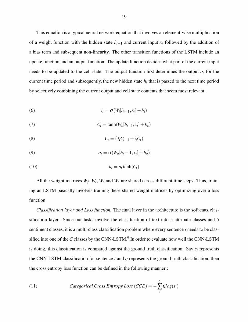
This equation is a typical neural network equation that involves an element-wise multiplication

of a weight function with the hidden state ht−1 and current input xt followed by the addition of

a bias term and subsequent non-linearity. The other transition functions of the LSTM include an

update function and an output function. The update function decides what part of the current input

needs to be updated to the cell state. The output function first determines the output ot for the

current time period and subsequently, the new hidden state ht that is passed to the next time period

by selectively combining the current output and cell state contents that seem most relevant.

it = σ(Wi[ht−1,xt ]+bi)(6)

Ct = tanh(Wc[ht−1,xt ]+bc)(7)

Ct = ( ftCt−1 + itCt)(8)

ot = σ(Wo[ht−1,xt ]+bo)(9)

ht = ot tanh(Ct)(10)

All the weight matrices Wf , Wi, Wc and Wo are shared across different time steps. Thus, train-

ing an LSTM basically involves training these shared weight matrices by optimizing over a loss

function.

Classification layer and Loss function. The final layer in the architecture is the soft-max clas-

sification layer. Since our tasks involve the classification of text into 5 attribute classes and 5

sentiment classes, it is a multi-class classification problem where every sentence i needs to be clas-

sified into one of the C classes by the CNN-LSTM.9 In order to evaluate how well the CNN-LSTM

is doing, this classification is compared against the ground truth classification. Say si represents

the CNN-LSTM classification for sentence i and ti represents the ground truth classification, then

the cross entropy loss function can be defined in the following manner :

Categorical Cross Entropy Loss (CCE) =−C

∑i

tilog(si)(11)

20

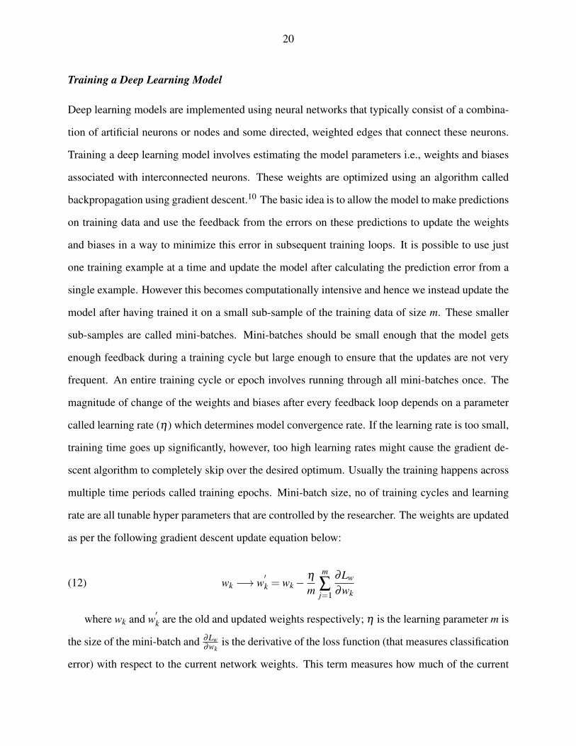
Training a Deep Learning Model

Deep learning models are implemented using neural networks that typically consist of a combina-

tion of artificial neurons or nodes and some directed, weighted edges that connect these neurons.

Training a deep learning model involves estimating the model parameters i.e., weights and biases

associated with interconnected neurons. These weights are optimized using an algorithm called

backpropagation using gradient descent.10 The basic idea is to allow the model to make predictions

on training data and use the feedback from the errors on these predictions to update the weights

and biases in a way to minimize this error in subsequent training loops. It is possible to use just

one training example at a time and update the model after calculating the prediction error from a

single example. However this becomes computationally intensive and hence we instead update the

model after having trained it on a small sub-sample of the training data of size m. These smaller

sub-samples are called mini-batches. Mini-batches should be small enough that the model gets

enough feedback during a training cycle but large enough to ensure that the updates are not very

frequent. An entire training cycle or epoch involves running through all mini-batches once. The

magnitude of change of the weights and biases after every feedback loop depends on a parameter

called learning rate (η) which determines model convergence rate. If the learning rate is too small,

training time goes up significantly, however, too high learning rates might cause the gradient de-

scent algorithm to completely skip over the desired optimum. Usually the training happens across

multiple time periods called training epochs. Mini-batch size, no of training cycles and learning

rate are all tunable hyper parameters that are controlled by the researcher. The weights are updated

as per the following gradient descent update equation below:

wk −→ w′k = wk−

η

m

m

∑j=1

∂Lw

∂wk(12)

where wk and w′k are the old and updated weights respectively; η is the learning parameter m is

the size of the mini-batch and ∂Lw∂wk

is the derivative of the loss function (that measures classification

error) with respect to the current network weights. This term measures how much of the current

21

error is attributable to the network weights.

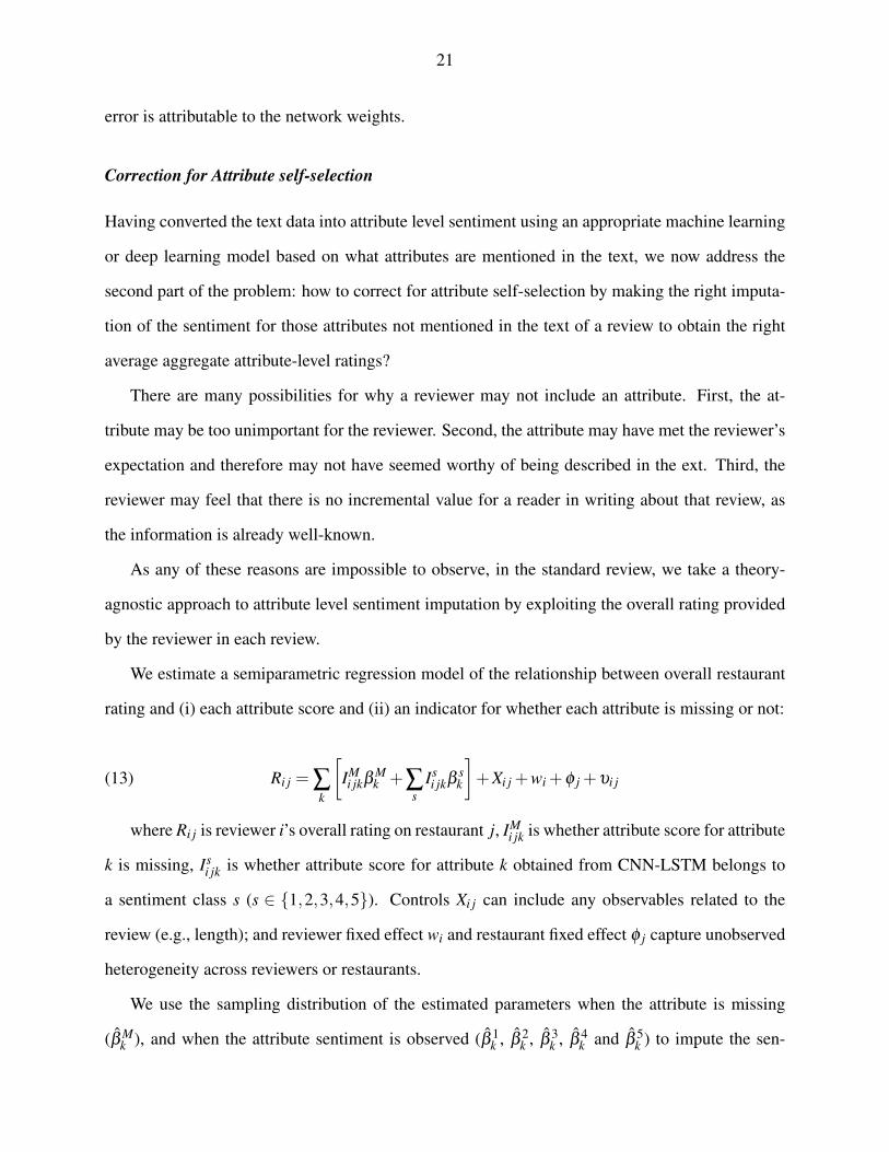
Correction for Attribute self-selection

Having converted the text data into attribute level sentiment using an appropriate machine learning

or deep learning model based on what attributes are mentioned in the text, we now address the

second part of the problem: how to correct for attribute self-selection by making the right imputa-

tion of the sentiment for those attributes not mentioned in the text of a review to obtain the right

average aggregate attribute-level ratings?

There are many possibilities for why a reviewer may not include an attribute. First, the at-

tribute may be too unimportant for the reviewer. Second, the attribute may have met the reviewer’s

expectation and therefore may not have seemed worthy of being described in the ext. Third, the

reviewer may feel that there is no incremental value for a reader in writing about that review, as

the information is already well-known.

As any of these reasons are impossible to observe, in the standard review, we take a theory-

agnostic approach to attribute level sentiment imputation by exploiting the overall rating provided

by the reviewer in each review.

We estimate a semiparametric regression model of the relationship between overall restaurant

rating and (i) each attribute score and (ii) an indicator for whether each attribute is missing or not:

Ri j = ∑k

[IMi jkβ

Mk +∑

sIsi jkβ

sk

]+Xi j +wi +φ j +υi j(13)

where Ri j is reviewer i’s overall rating on restaurant j, IMi jk is whether attribute score for attribute

k is missing, Isi jk is whether attribute score for attribute k obtained from CNN-LSTM belongs to

a sentiment class s (s ∈ {1,2,3,4,5}). Controls Xi j can include any observables related to the

review (e.g., length); and reviewer fixed effect wi and restaurant fixed effect φ j capture unobserved

heterogeneity across reviewers or restaurants.

We use the sampling distribution of the estimated parameters when the attribute is missing

(β Mk ), and when the attribute sentiment is observed (β 1

k , β 2k , β 3

k , β 4k and β 5

k ) to impute the sen-

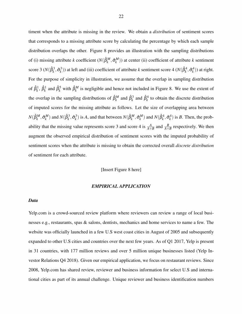
22

timent when the attribute is missing in the review. We obtain a distribution of sentiment scores

that corresponds to a missing attribute score by calculating the percentage by which each sample

distribution overlaps the other. Figure 8 provides an illustration with the sampling distributions

of (i) missing attribute k coefficient (N(β Mk , σM

k )) at center (ii) coefficient of attribute k sentiment

score 3 (N(β 3k , σ

3k )) at left and (iii) coefficient of attribute k sentiment score 4 (N(β 4

k , σ4k )) at right.

For the purpose of simplicity in illustration, we assume that the overlap in sampling distribution

of β 1k , β 1

k and β 5k with β M

k is negligible and hence not included in Figure 8. We use the extent of

the overlap in the sampling distributions of β Mk and β 3

k and β 4k to obtain the discrete distribution

of imputed scores for the missing attribute as follows. Let the size of overlapping area between

N(β Mk , σM

k ) and N(β 3k , σ

3k ) is A, and that between N(β M

k , σMk ) and N(β 4

k , σ4k ) is B. Then, the prob-

ability that the missing value represents score 3 and score 4 is AA+B and B

A+B respectively. We then

augment the observed empirical distribution of sentiment scores with the imputed probability of

sentiment scores when the attribute is missing to obtain the corrected overall discrete distribution

of sentiment for each attribute.

[Insert Figure 8 here]

EMPIRICAL APPLICATION

Data

Yelp.com is a crowd-sourced review platform where reviewers can review a range of local busi-

nesses e.g., restaurants, spas & salons, dentists, mechanics and home services to name a few. The

website was officially launched in a few U.S west coast cities in August of 2005 and subsequently

expanded to other U.S cities and countries over the next few years. As of Q1 2017, Yelp is present

in 31 countries, with 177 million reviews and over 5 million unique businesses listed (Yelp In-

vestor Relations Q4 2018). Given our empirical application, we focus on restaurant reviews. Since

2008, Yelp.com has shared review, reviewer and business information for select U.S and interna-

tional cities as part of its annual challenge. Unique reviewer and business identification numbers

23

in the data helps create a two-way panel of reviews at reviewer and business level. We use a panel

data of Yelp reviews from 5 major U.S cities— Las Vegas, Pittsburgh, Charlotte, Phoenix and

Cleveland which are geographically well-distributed and have Yelp review data from as early as

2008–allowing us to have long enough panel data. For each review, we observe overall rating,

textual evaluation and date of posting as well as information about business characteristics (e.g.,

cuisine, price range, address, name) and reviewer characteristics (e.g., experience with Yelp, Elite

membership).

We only work with restaurant reviews and use the full dataset of 1.2 million restaurant reviews

for identifying high-frequency words and lexicon construction.11 We then use this restaurant-

specific review dataset to build a vocabulary of 8,575 high frequency noun and noun phrases,

verbs, adjectives and adverbs as described earlier in the model section. These words comprise of

4,622 nouns and noun phrases and 2,245 adjectives and adverbs that could be easily classified into

attribute and sentiment words respectively. However, the 1,708 verbs and verb phrases could be

either attribute or sentiment words. For e.g., verbs like “greeted” or “served” are clearly associated

with the attribute service whereas some verbs like “impressed” or “expected” refer to sentiment.

To resolve this ambiguity, we used human taggers on Mturk to classify these verb and verb phrases

into attributes and sentiment words.12

Human taggers classify attribute words into 5 attribute classes — food, service, price, ambiance

and location and sentiment words into 5 levels of sentiment from extremely negative to extremely

positive. Food attribute represents menu items served (e.g., salad, chicken, sauce, drinks, cock-

tails); service stands for employee behavior, friendliness or timeliness (e.g., waiter, serve, greeted);

price refers to value for money, menu price or promotional offers (e.g., deal, bill); ambiance rep-

resents decor or look and feel (e.g., noise, view); and location captures neighborhood, parking

and general convenience (e.g., airport, office). Examples of sentiment words include “delicious”

or “not fresh” for food; “responsive” or “slow” for service; “bargain” or “expensive” for price;

“elegant” or “crowded” for ambiance; “convenient”, or “unsafe” for location. Table 3 shows the

most frequent attribute and sentiment words identified.

24

[Insert Table 3 here ]

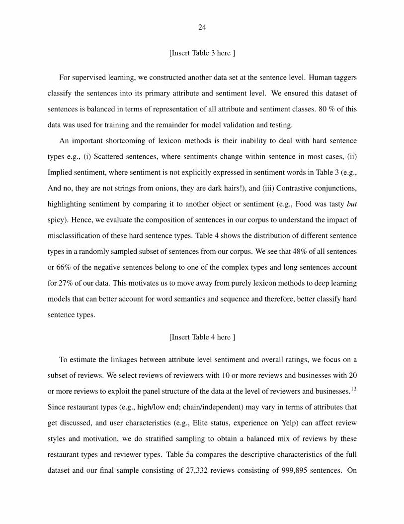
For supervised learning, we constructed another data set at the sentence level. Human taggers

classify the sentences into its primary attribute and sentiment level. We ensured this dataset of

sentences is balanced in terms of representation of all attribute and sentiment classes. 80 % of this

data was used for training and the remainder for model validation and testing.

An important shortcoming of lexicon methods is their inability to deal with hard sentence

types e.g., (i) Scattered sentences, where sentiments change within sentence in most cases, (ii)

Implied sentiment, where sentiment is not explicitly expressed in sentiment words in Table 3 (e.g.,

And no, they are not strings from onions, they are dark hairs!), and (iii) Contrastive conjunctions,

highlighting sentiment by comparing it to another object or sentiment (e.g., Food was tasty but

spicy). Hence, we evaluate the composition of sentences in our corpus to understand the impact of

misclassification of these hard sentence types. Table 4 shows the distribution of different sentence

types in a randomly sampled subset of sentences from our corpus. We see that 48% of all sentences

or 66% of the negative sentences belong to one of the complex types and long sentences account

for 27% of our data. This motivates us to move away from purely lexicon methods to deep learning

models that can better account for word semantics and sequence and therefore, better classify hard

sentence types.

[Insert Table 4 here ]

To estimate the linkages between attribute level sentiment and overall ratings, we focus on a

subset of reviews. We select reviews of reviewers with 10 or more reviews and businesses with 20

or more reviews to exploit the panel structure of the data at the level of reviewers and businesses.13

Since restaurant types (e.g., high/low end; chain/independent) may vary in terms of attributes that

get discussed, and user characteristics (e.g., Elite status, experience on Yelp) can affect review

styles and motivation, we do stratified sampling to obtain a balanced mix of reviews by these

restaurant types and reviewer types. Table 5a compares the descriptive characteristics of the full

dataset and our final sample consisting of 27,332 reviews consisting of 999,895 sentences. On

25

average, reviewers in our sample have longer experience on Yelp and post more and shorter reviews

than those in the full data, but they are fairly representative in terms of average rating.

[Insert Table 5a here ]

Table 5b provides the number of businesses, reviews and the summary of star rating by a

restaurant’s price range, chain/non-chain and reviewer type in terms of Elite status. Our sample

has almost an equal mix of chain and independent restaurants but independent restaurants get more

reviews with higher ratings on average. Low-end and high-end restaurants, or Elite and non-Elite

users do not show much difference in terms of average star rating.

[Insert Table 5b here ]

Table 6 describes how frequently various attributes are mentioned in reviews by restaurant

and reviewer types. Food and Service are most likely to be evaluated across all restaurant types.

High-end restaurant reviews are more likely to mention attributes other than location than low-end

ones. All attributes are always more mentioned in Elite reviewers’ posts. Comparing low-end and

high-end restaurants, we argue that missingness of these attributes does not necessarily capture a

lack of importance, but is related to how much customers can learn about the attribute ex ante and

would find its quality surprising after experiences. For example, while price is expected to be more

important to low-end restaurant reviewers, it is more likely to be mentioned in high-end restaurant

reviews. We claim that value for money would be evaluated only after experience in high-end

restaurants, whereas low-end restaurant customers tend to have fairly precise expectations on it.

Thus, we need careful interpretations on missing attributes separately by restaurant or reviewer

types.

[Insert Table 6 here ]

RESULTS

We describe two main sets of results — (i) performance comparison of various text mining methods

and (ii) the impact of correcting for attribute self-selection.

26

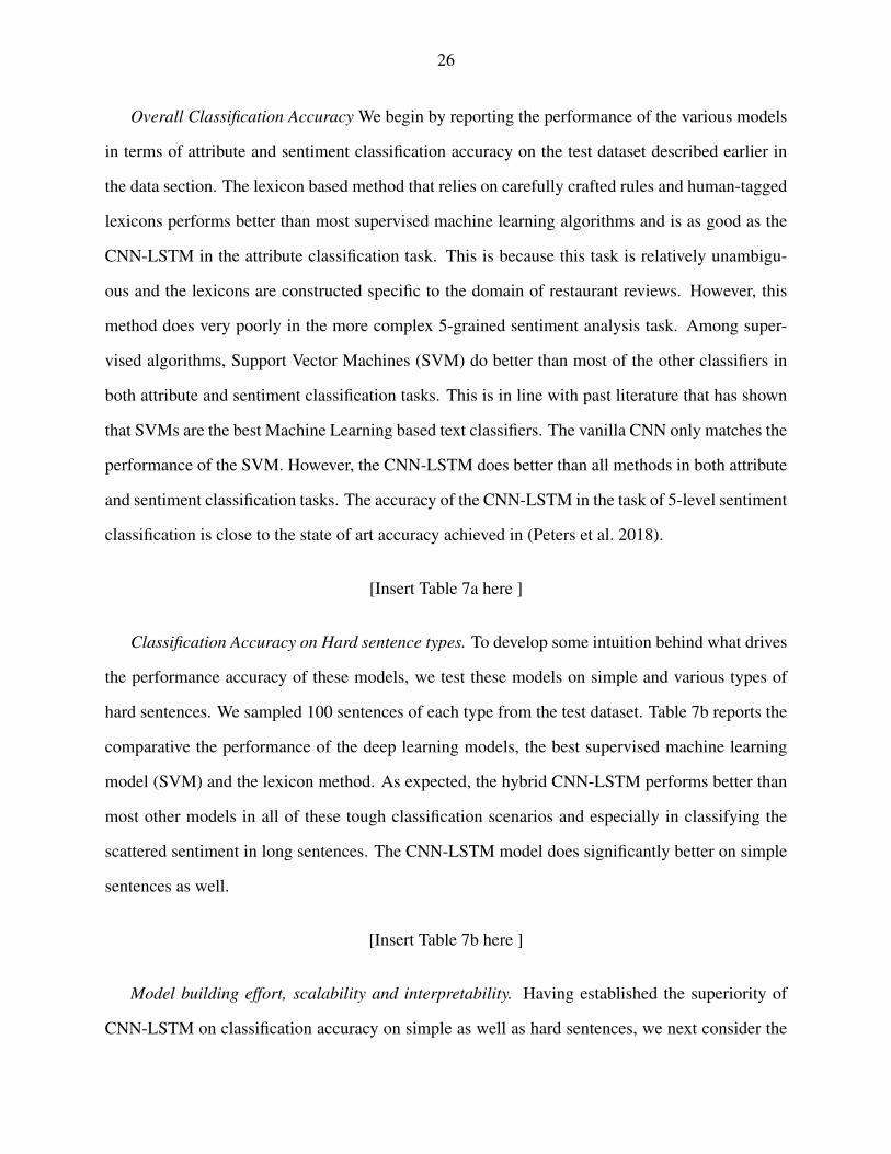
Overall Classification Accuracy We begin by reporting the performance of the various models

in terms of attribute and sentiment classification accuracy on the test dataset described earlier in

the data section. The lexicon based method that relies on carefully crafted rules and human-tagged

lexicons performs better than most supervised machine learning algorithms and is as good as the

CNN-LSTM in the attribute classification task. This is because this task is relatively unambigu-

ous and the lexicons are constructed specific to the domain of restaurant reviews. However, this

method does very poorly in the more complex 5-grained sentiment analysis task. Among super-

vised algorithms, Support Vector Machines (SVM) do better than most of the other classifiers in

both attribute and sentiment classification tasks. This is in line with past literature that has shown

that SVMs are the best Machine Learning based text classifiers. The vanilla CNN only matches the

performance of the SVM. However, the CNN-LSTM does better than all methods in both attribute

and sentiment classification tasks. The accuracy of the CNN-LSTM in the task of 5-level sentiment

classification is close to the state of art accuracy achieved in (Peters et al. 2018).

[Insert Table 7a here ]

Classification Accuracy on Hard sentence types. To develop some intuition behind what drives

the performance accuracy of these models, we test these models on simple and various types of

hard sentences. We sampled 100 sentences of each type from the test dataset. Table 7b reports the

comparative the performance of the deep learning models, the best supervised machine learning

model (SVM) and the lexicon method. As expected, the hybrid CNN-LSTM performs better than

most other models in all of these tough classification scenarios and especially in classifying the

scattered sentiment in long sentences. The CNN-LSTM model does significantly better on simple

sentences as well.

[Insert Table 7b here ]

Model building effort, scalability and interpretability. Having established the superiority of

CNN-LSTM on classification accuracy on simple as well as hard sentences, we next consider the

27

performance of the different models on three other dimensions: model building effort, scalability

and interpretability. For Model Building Effort, we measure the time needed for lexicon construc-

tion in the lexicon methods. Equivalently, we measure the time needed for test data creation and

model fitting for supervised learning methods. Scalability is a measure of the increase in deploy-

ment time as a function of data size. In our empirical setting, deployment time is the time for a

constructed model to classify new sentences. Interpretability refers to how well a machine clas-

sifier can explain the reasoning or logic behind its classifications (Doshi-Velez and Kim 2017).

In general, text mining methods differ in their strengths and weakness across various dimensions,

there is no one method that is superior in all dimensions. Figure 9 graphically summarizes all of

the metrics (including classification accuracy) we use for performance evaluation of models.

[Insert Figure 9 here ]

Lexicon models take approximately 175-180 hours of construction time. Most of the time

is spent on human-tagging of the 8575 attribute and sentiment words into specific classes using

Amazon’s Mechanical Turk. Similarly, the creation of training and test data sets for the super-

vised learning algorithms takes approximately 100 hours.14 However, once created, we could use

the same dataset to train and test a variety of machine learning and deep learning classifiers (e.g.,

SVM, Random Forest, Naive Bayes, CNN, LSTM and CNN-LSTM). After generating the train-

ing data, supervised learning models (including the deep learning models) need time for hyper

parameter tuning and model training. Though this is an iterative process, all deep learning models

take less than 10 minutes (in a quad core processor) for completing one training cycle and hence

model calibration can be completed in 6-7 hours. Thus, model building is time-consuming for all

algorithms but is a one-time activity.

The more time-sensitive metric is scalability i.e. the time required for a trained model to

classify new examples. With respect to the scalability metric, the deep learning classifiers clearly

outperform the lexicon based classifiers with the machine learning classifiers in between the other

two. The main reason is the “look-up” method employed by lexicon based methods. Every word

in a sentence needs to be sequentially searched through the entire lexicon to determine its class.

28

Hence, the lexicon methods need several hours to classify our corpus of 27,332 reviews comprising

of 999,885 sentences. On the other hand, deep learning models are able to classify our entire review

dataset comprising in approximately 18- 20 minutes.

Though the CNN-LSTM model outperforms all the other models in accuracy and scalability,

however, it falls short in terms of interpretability with respect to lexicon methods. However, to

develop some intuition for what drives the performance of the deep learning models, we evaluate

performance of different models on “hard” sentence types.

Sensitivity to training data size and hyper parameter tuning. For purposes of exposition, and

highlighting the key results, we reported the results of the various parameters based on the best

tuned hyper parameters and the optimal training data size. However, we now report the sensitivity

of the models to these hyper parameters to help the reader appreciate the tradeoffs.

To save space, we discuss hyper parameter sensitivity for the best performing CNN-LSTM

model but it is applicable for all the deep learning models. We started our tuning using guidelines

from (Zhang and Wallace 2015) which finds that the most important hyper parameters for text clas-

sification tasks are the number and size of filters and the word embeddings used. We use filters of

kernel sizes [1,2,3,4,5] for both attribute and sentiment classification but found that smaller kernel

sizes of 1, 2 give better test accuracy for attribute classification whereas sentiment classification

benefits from having higher order n-grams (3, 4 and 5-grams) along with uni-grams and bi-grams.

Different word embeddings can work for different types of tasks and domains depending on com-

plexity and domain similarity. We find that 100- dimensional GloVe embeddings work well for the

attribute classification task whereas 300- dimensional GloVe embeddings do better for the senti-

ment analysis task. This is most likely because capturing long dependencies is more important in

the relatively complex fine-grained sentiment analysis task. The other important hyper parameters

are the optimizer used to control the learning rate and the regularization technique used. On this,

we follow the best practice of using an adaptive instead of a fixed learning rate optimizer called

ADAM (Kingma and Ba 2014) and the dropout regularization technique (Srivastava et al. 2014)

with a dropout rate of 0.4 that reduces over-fitting by randomly dropping some units(along with

29

interconnections) during training. We train the model in mini-batches of size 32.

Table 7c shows the sensitivity of our best performing model CNN-LSTM to changes in the

most important hyper parameters — filter size (that impacts size of n-grams captured) and size

of the word embedding used (which captures the richness of the contextual information of the

embedding)

[Insert Table 7c here ]

Fig 10a shows how size of the training data impacts classification accuracy for the attribute

classification task. The impact is similar for the sentiment classification task. We also study the

impact of number of training epochs and batch-size on the test accuracy achieved. Batch-size

does not have a huge impact on test accuracy and the model does not improve much after training

for 30 epochs. In fact, after 30 epochs of training, test accuracy declines while training accuracy

continues to increase which is a sign of over fitting.

[Insert Figure 10 here ]

Attribute Level Ratings Accounting for Self-Selection

As explained earlier, estimating the semiparametric regression in equation 13 can serve to address

the issue of attribute self-selection. In empirical analysis, we consider whether the interpretation

of missing attributes varies by high and low-end restaurants, by adding interaction terms with

restaurant type to estimate equation 14:15

Ri j = ∑p∈{L,H}

Ipj ∑

k

[IMi jkβ

Mpk +∑

sIsi jkβ

spk

]+Xi j +wi +φ j +υi j(14)

where Ipj indicates restaurant j’s type p (p ∈ {H,L}).

Given the large number of coefficients in the regression, we present the attribute level coeffi-

cients associated with each sentiment score and the missing attribute in graphs.

[Insert Figures 11a and 11b here]

30

Figures 11a and 11b plots βM,pk , β

1,pk , β

2,pk , β

3,pk , β

4,pk and β

5,pk (p ∈ H,L) for each attribute

and their 95% confidence intervals for low-end and high-end restaurant reviews, respectively; and

food, service, price, ambiance and location attributes are analyzed in order. The coefficients show

the impact of each attribute sentiment score on overall rating, controlling for all other attribute

sentiment scores, fixed effects and other control variables.16

Before discussing the imputation of missing values, we note from Figure 8 that based on the

range of estimates of βk, as expected, food and service have much higher impact on overall ratings

relative to the other three variables. Thus in fact, there is justification for the intuition that the most

important features are the ones that are discussed most in online text reviews.

Nevertheless, it is still an empirical question as to what it means when the attribute is missing

in text reviews. Let us illustrate this with the food attribute. When food attribute is missing,

the effect is close to when the sentiment score is 4 for both low-end and high-end restaurants.

But the 95% confidence interval of β Mf ood is much smaller for the low end relative to high end

restaurants. Thus the sampling distribution of β Mf ood for low end restaurant overlaps only with the

sampling distribution of β 4f ood , and therefore we impute a value of 4 with probability 1 in this

case. In contrast, the sampling distribution of β Mf ood for the high end restaurants, overlaps with the

sampling distribution of β 2f ood , β 3

f ood , β 4f ood and β 5

f ood . As discussed in Figure 8, we then use this

overlapping area to determine the probabilities of different sentiment level to be imputed to β Mf ood

for the low and high end restaurants. Specifically, we find that the probabilities are 0.11 for score

2, 0.24 for score 3, 0.33 for score 4 and 0.32 for score 5 for high-end restaurant reviews.

Table 8 lists imputation values and probabilities for all attributes for low-end and high-end

restaurant reviews.

[Insert Table 8 here ]

Given how different levels of sentiment are weighted for missing, we then simulate draws from

this distribution of sentiment for missing values for the proportion of missing reviews to obtain

an aggregate corrected rating for each attribute. We illustrate the results of such imputation for a

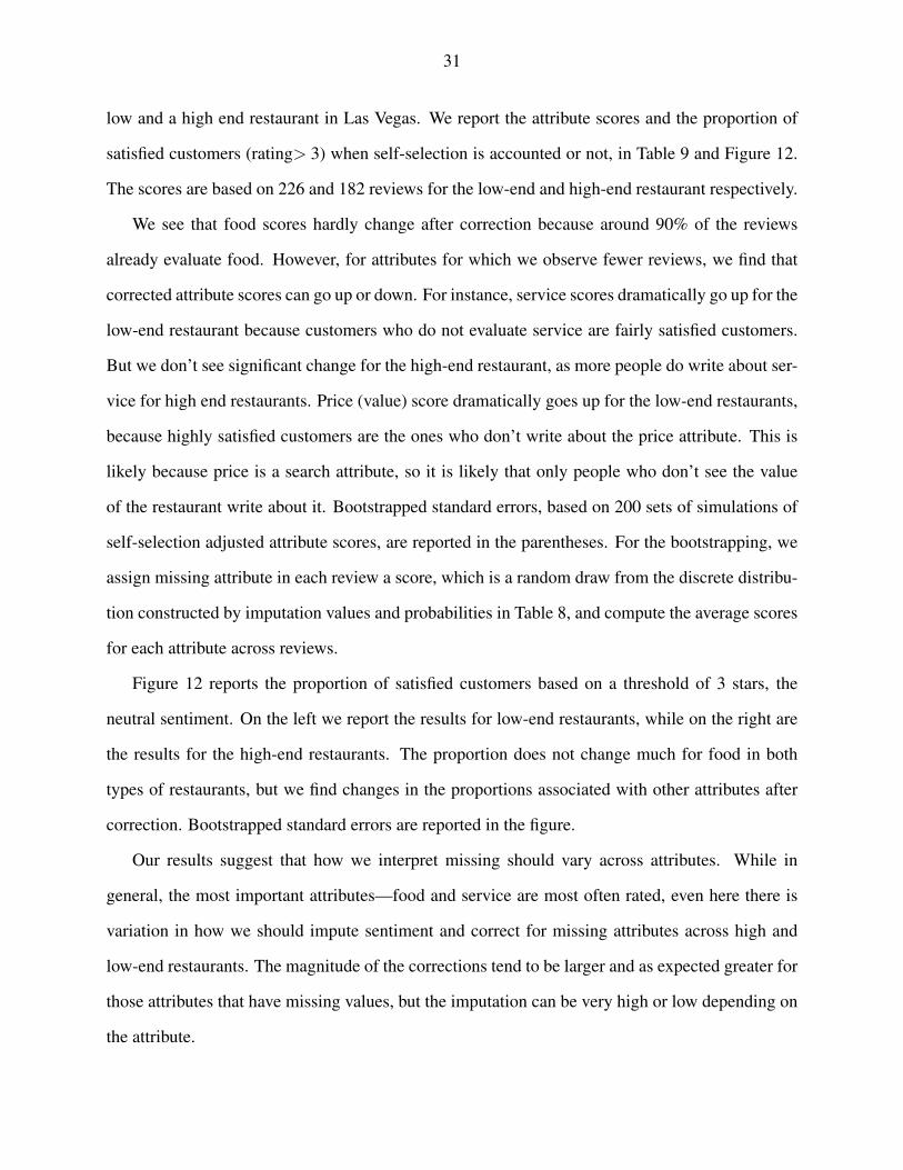
31

low and a high end restaurant in Las Vegas. We report the attribute scores and the proportion of

satisfied customers (rating> 3) when self-selection is accounted or not, in Table 9 and Figure 12.

The scores are based on 226 and 182 reviews for the low-end and high-end restaurant respectively.

We see that food scores hardly change after correction because around 90% of the reviews

already evaluate food. However, for attributes for which we observe fewer reviews, we find that

corrected attribute scores can go up or down. For instance, service scores dramatically go up for the

low-end restaurant because customers who do not evaluate service are fairly satisfied customers.

But we don’t see significant change for the high-end restaurant, as more people do write about ser-

vice for high end restaurants. Price (value) score dramatically goes up for the low-end restaurants,

because highly satisfied customers are the ones who don’t write about the price attribute. This is

likely because price is a search attribute, so it is likely that only people who don’t see the value

of the restaurant write about it. Bootstrapped standard errors, based on 200 sets of simulations of

self-selection adjusted attribute scores, are reported in the parentheses. For the bootstrapping, we

assign missing attribute in each review a score, which is a random draw from the discrete distribu-

tion constructed by imputation values and probabilities in Table 8, and compute the average scores

for each attribute across reviews.

Figure 12 reports the proportion of satisfied customers based on a threshold of 3 stars, the

neutral sentiment. On the left we report the results for low-end restaurants, while on the right are

the results for the high-end restaurants. The proportion does not change much for food in both

types of restaurants, but we find changes in the proportions associated with other attributes after

correction. Bootstrapped standard errors are reported in the figure.

Our results suggest that how we interpret missing should vary across attributes. While in

general, the most important attributes—food and service are most often rated, even here there is

variation in how we should impute sentiment and correct for missing attributes across high and

low-end restaurants. The magnitude of the corrections tend to be larger and as expected greater for

those attributes that have missing values, but the imputation can be very high or low depending on

the attribute.

32

CONCLUSION

This paper introduces the problem of inferring attribute level sentiment from text data into the

marketing literature. Mining unstructured data like images, audio and text from various social me-

dia and review platforms, marketing content, and email for insight is growing in importance for a

variety of applications, and there has been a surge of interest among marketing scholars in mining

text data over the last decade. But these papers have typically treated text documents as “bags of

words,” that do not account for how structural characteristics of language affect meaning. This

paper introduces a deep learning CNN-LSTM hybrid model that accounts for the spatial and se-

quential structure of language to more accurately infer attribute level sentiment from online review

data. The CNN-LSTM deep learning model does especially better with respect to well-known

hard to classify sentences that involve scattered sentiments, implied sentiment and contrastive con-

junctions, relative to other lexicon, machine learning and deep learning methods. Remarkably, the

model compares very favorably not only on accuracy, but also training speed, model building and

deployment time, relative to the traditional lexicon based method.

Second, it addresses the issue that reviewers self-select what attributes to mention in their

reviews. We question the standard assumption that when an attribute is not mentioned, it is because

the attribute is not important. We develop a sentiment imputation procedure when attributes are

missing to obtain corrected estimates of attribute level restaurant sentiment rating.

We conclude with a discussion of assumptions and issues that we abstracted away that could

be a focus in future research. We assumed that reviewers discuss only one attribute per sentence.

While this assumption is mostly satisfied in review data, it would be worthwhile to generalize our

model to accommodate settings where multiple attributes per sentence are common. We assumed

that all sentences have equal weight when computing overall sentiment. Though this assumption

is commonly used in lexicon based models, it would be worth exploring the empirical value of a

more flexible weighting scheme based on certain observable characteristics of sentences such as

length and frequency of positive/ negative words.

33

Finally, we abstracted away from reviewer selection in terms of who write reviews relative

to those who eat at restaurants and the problem of fake reviews and review shading. While this

was reasonable in our application, because Yelp does not also make corrections for these issues in

reporting overall rating, it can be valuable to develop corrected ratings accounting for these issues

in other contexts.

34

REFERENCES

Aggarwal CC, Zhai C (2012) Mining text data (Springer Science & Business Media).

Berger J, Sorensen AT, Rasmussen SJ (2010) Positive effects of negative publicity: When negative

reviews increase sales. Marketing Science 29(5):815–827.

Boulding W, Kalra A, Staelin R, Zeithaml VA (1993) A dynamic process model of sevice quality:

from expectations to behavioral intentions. Journal of marketing research 30(1):7–27.

Buschken J, Allenby GM (2016) Sentence-based text analysis for customer reviews. Marketing

Science 35(6):953–975.

Chevalier JA, Mayzlin D (2006) The effect of word of mouth on sales: Online book reviews.

Journal of marketing research 43(3):345–354.

Chung J, Rao VR (2003) A general choice model for bundles with multiple-category products:

Application to market segmentation and optimal pricing for bundles. Journal of Marketing

Research 40(2):115–130.

Churchill Jr GA, Surprenant C (1982) An investigation into the determinants of customer satisfac-

tion. Journal of marketing research 491–504.

Culotta A, Cutler J (2016) Mining brand perceptions from twitter social networks. Marketing sci-

ence 35(3):343–362.

Dhar V, Chang EA (2009) Does chatter matter? the impact of user-generated content on music

sales. Journal of Interactive Marketing 23(4):300–307.

Doshi-Velez F, Kim B (2017) Towards a rigorous science of interpretable machine learning. arXiv

preprint arXiv:1702.08608 .

Duan W, Gu B, Whinston AB (2008) Do online reviews matter?—an empirical investigation of

panel data. Decision support systems 45(4):1007–1016.

Feldman R (2013) Techniques and applications for sentiment analysis. Communications of the

ACM 56(4):82–89.

35

Ganu G, Elhadad N, Marian A (2009) Beyond the stars: improving rating predictions using review

text content. WebDB, volume 9, 1–6 (Citeseer).

Ghose A, Ipeirotis PG (2007) Designing novel review ranking systems: predicting the usefulness

and impact of reviews. Proceedings of the ninth international conference on Electronic com-

merce, 303–310 (ACM).

Goodfellow IJ, Bengio Y, Courville AC (2016) Deep Learning. Adaptive computation and machine

learning (MIT Press).

Harris ZS (1954) Distributional structure. Word 10(2-3):146–162.

Hochreiter S, Schmidhuber J (1997) Long short-term memory. Neural Comput. 9(8):1735–1780,

ISSN 0899-7667.

Hollenbeck B (2018) Online reputation mechanisms and the decreasing value of chain affiliation.

Journal of Marketing Research 55(5):636–654.

Joachims T (2002) Learning to classify text using support vector machines, volume 668 (Springer

Science & Business Media).

Kim Y (2014) Convolutional neural networks for sentence classification. preprint arXiv:1408.5882

.

Kingma DP, Ba J (2014) Adam: A method for stochastic optimization. arXiv preprint

arXiv:1412.6980 .

Lappas T, Sabnis G, Valkanas G (2016) The impact of fake reviews on online visibility: A vulner-

ability assessment of the hotel industry. Information Systems Research 27(4):940–961.

LaTour SA, Peat NC (1979) Conceptual and methodological issues in consumer satisfaction re-

search. ACR North American Advances .

Lee TY, Bradlow ET (2011) Automated marketing research using online customer reviews. Journal

of Marketing Research 48(5):881–894.

Li X, Hitt LM (2008) Self-selection and information role of online product reviews. Information

Systems Research 19(4):456–474.

36

Liu B, et al. (2010) Sentiment analysis and subjectivity. Handbook of natural language processing

2(2010):627–666.

Liu L, Dzyabura D, Mizik N (2018a) Visual listening in: Extracting brand image portrayed on

social media. Workshops at the Thirty-Second AAAI Conference on Artificial Intelligence.

Liu X, Lee D, Srinivasan K (2018b) Large scale cross-category analysis of consumer review con-

tent on sales conversion leveraging deep learning. Workshops at the Thirty-Second AAAI Con-

ference on Artificial Intelligence.

Luca M (2016) Reviews, reputation, and revenue: The case of yelp. com .

Luca M, Zervas G (2016) Fake it till you make it: Reputation, competition, and yelp review fraud.

Management Science 62(12):3412–3427.

Mayzlin D, Dover Y, Chevalier J (2014) Promotional reviews: An empirical investigation of online

review manipulation. American Economic Review 104(8):2421–55.

Mikolov T, Sutskever I, Chen K, Corrado GS, Dean J (2013) Distributed representations of words

and phrases and their compositionality. Advances in neural information processing systems,

3111–3119.

Nair V, Hinton GE (2010) Rectified linear units improve restricted boltzmann machines. Proceed-

ings of the 27th International Conference on International Conference on Machine Learning,

807–814, ICML’10, ISBN 978-1-60558-907-7.

Netzer O, Feldman R, Goldenberg J, Fresko M (2012) Mine your own business: Market-structure

surveillance through text mining. Marketing Science 31(3):521–543.

Nielsen FA (2011) A new anew: Evaluation of a word list for sentiment analysis in microblogs.

arXiv preprint arXiv:1103.2903 .

Onishi H, Manchanda P (2012) Marketing activity, blogging and sales. International Journal of

Research in Marketing 29(3):221–234.

Pak A, Paroubek P (2010) Twitter as a corpus for sentiment analysis and opinion mining. LREc,

volume 10.

37

Parasuraman A, Zeithaml VA, Berry LL (1988) Servqual: A multiple-item scale for measuring

consumer perc. Journal of retailing 64(1):12.

Pennington J, Socher R, Manning C (2014) Glove: Global vectors for word representation.

Proceedings of the 2014 conference on empirical methods in natural language processing

(EMNLP), 1532–1543.

Peters ME, Neumann M, Iyyer M, Gardner M, Clark C, Lee K, Zettlemoyer L (2018) Deep con-

textualized word representations. Proc. of NAACL.

Puranam D, Narayan V, Kadiyali V (2017) The effect of calorie posting regulation on consumer

opinion: a flexible latent dirichlet allocation model with informative priors. Marketing Science

36(5):726–746.

Sebastiani F (2002) Machine learning in automated text categorization. ACM computing surveys

(CSUR) 34(1):1–47.

Socher R, Perelygin A, Wu J, Chuang J, Manning CD, Ng A, Potts C (2013) Recursive deep models

for semantic compositionality over a sentiment treebank. Proceedings of the 2013 conference

on empirical methods in natural language processing, 1631–1642.

Srivastava N, Hinton G, Krizhevsky A, Sutskever I, Salakhutdinov R (2014) Dropout: a simple

way to prevent neural networks from overfitting. The Journal of Machine Learning Research

15(1):1929–1958.

Taboada M, Brooke J, Tofiloski M, Voll K, Stede M (2011) Lexicon-based methods for sentiment

analysis. Computational linguistics 37(2):267–307.

Timoshenko A, Hauser JR (2018) Identifying customer needs from user-generated content. Mar-

keting Science (Forthcoming) .

Tirunillai S, Tellis GJ (2014) Mining marketing meaning from online chatter: Strategic brand anal-

ysis of big data using latent dirichlet allocation. Journal of Marketing Research 51(4):463–

479.

Vesset D, Schubmehl D (2016) Idc futurescape: Worldwide big data and analytics, predictions.

38

International Data Corporation .

Wang H, Lu Y, Zhai C (2010) Latent aspect rating analysis on review text data: a rating regression

approach. Proceedings of the 16th ACM SIGKDD international conference on Knowledge

discovery and data mining, 783–792 (ACM).

Weston J, Ratle F, Mobahi H, Collobert R (2012) Deep learning via semi-supervised embedding.

Neural Networks: Tricks of the Trade, 639–655 (Springer).

Wilkie WL, Pessemier EA (1973) Issues in marketing’s use of multi-attribute attitude models.

Journal of Marketing research 428–441.

Xu K, Ba J, Kiros R, Cho K, Courville AC, Salakhutdinov R, Zemel RS, Bengio Y (2015) Show,

attend and tell: Neural image caption generation with visual attention. CoRR abs/1502.03044.

Zhang Y, Wallace BC (2015) A sensitivity analysis of (and practitioners’ guide to) convolutional

neural networks for sentence classification. CoRR abs/1510.03820.

Zhou C, Sun C, Liu Z, Lau F (2015) A c-lstm neural network for text classification. preprint

arXiv:1511.08630 .

39

ENDNOTES

1. Zagat, one of the oldest crowd-sourced review platforms, collects restaurant reviews across four

attributes: food, decor, service, and cost, has 250,000 reviewers from over 40 US cities. This is

much smaller in magnitude to Yelp’s 177 million reviews (by the end of 2018) from millions of

reviewers around the world.

2. As a by-product, obtaining such attribute level ratings can also help businesses and researchers

measure the extent to which different attributes drive overall ratings (customer satisfaction).

3. For completeness, we also estimate some bag-of-words based supervised machine learning mod-

els e.g., Support-Vector-Machine (SVM), Naive Bayes and Logistic Regression as they have been

used for text classification in the past. Aggarwal and Zhai (2012), Sebastiani (2002) provide a

good review of these methods.

4. AFINN lexicon (Nielsen 2011) and Stanford Sentiment Treebank (Socher et al. 2013) have

words and phrases with 5-levels of sentiment classification , however, they are built on Twitter and

rotten.tomatoes.com movie review dataset respectively and have limited overlap with our domain.

5. Pre-processing can remove some subtle sentiment cues like exclamation marks and use of

capital letters. However, it helps in standardization of the text and simplifies succeeding tasks like

vocabulary generation. Besides, there is no consensus about what sentiments are communicated

by punctuation, hence, we remove them during pre-processing, as is commonly done in lexicon

based text analysis literature (e.g., Liu et al. (2010), Tirunillai and Tellis (2014).)

6. Many commercial parts of speech (POS) taggers are available e.g. Stanford POS Tagger, Illinois

POS tagger etc. We used the averaged perceptron tagger from the open-source Python natural

language processing library NLTK that does POS tagging for individual words.

7. The simplest method to form numeric vectors from words is a one-hot representation which

40

means that if there are V words in the vocabulary; each word is represented as a V ×1 dimensional

vector where exactly one of the bits is 1 and rest are zero. Such a representation is not scalable

for large vocabularies and also stores no semantic information about words. Another option is

to only take into account word frequency and simply convert words into numbers based on some

normalized frequency score like tf-idf.

8. These embeddings have been trained on different corpus like Wikipedia dumps, Gigaword news

dataset and web data from Common Crawl and have more than 5 billion unique tokens.

9. We allow for a sixth class when the sentence is not associated with any of the five attribute

classes.

10. For a detailed review of gradient descent algorithms refer (Goodfellow et al. 2016).

11. Category-specific lexicons lead to higher accuracy in both attribute discovery and sentiment

analysis.

12. The entire dictionary of attribute or sentiment words we identified is available upon request.

13. This restriction of 10 or more reviews also allows us to eliminate human or bot-generated fake

reviews, which are mostly generated by users with one or only a few number of reviews. Luca and

Zervas (2016) document that a larger number of reviews by a Yelp user is negatively correlated to

the probability of his reviews getting filtered as spam by Yelp.

14. A human tagger takes around 1 minute to classify every word and 2-3 minutes to classify full

sentences

15. We also considered observed heterogeneity in terms of restaurant types (e.g., chain/non-chain)

and reviewer types (e.g., Elite/non-Elite). We present the findings associated with low-end/high-

end restaurants for illustration.

16. Note that β1,pk is the baseline set to zero in the regression, so it has no standard error.

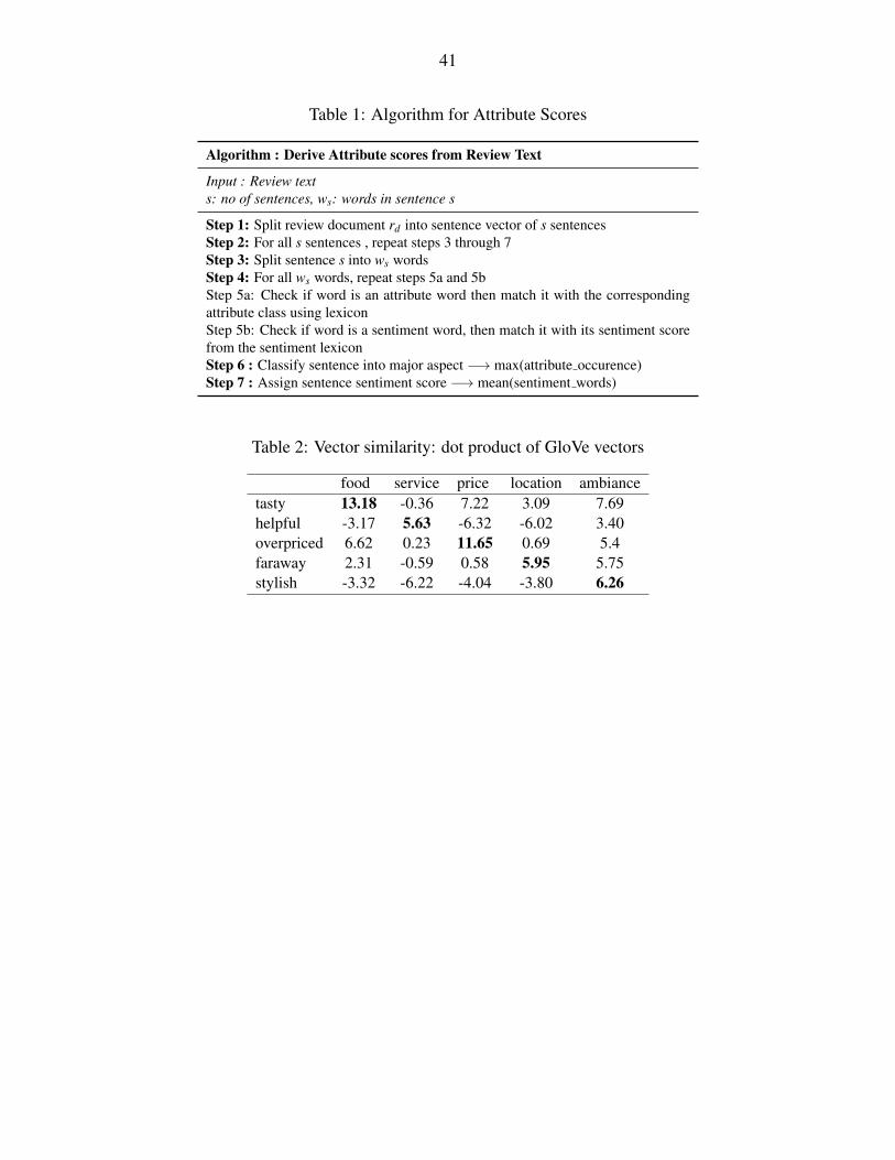
41

Table 1: Algorithm for Attribute Scores

Algorithm : Derive Attribute scores from Review Text

Input : Review texts: no of sentences, ws: words in sentence s

Step 1: Split review document rd into sentence vector of s sentencesStep 2: For all s sentences , repeat steps 3 through 7Step 3: Split sentence s into ws wordsStep 4: For all ws words, repeat steps 5a and 5bStep 5a: Check if word is an attribute word then match it with the correspondingattribute class using lexiconStep 5b: Check if word is a sentiment word, then match it with its sentiment scorefrom the sentiment lexiconStep 6 : Classify sentence into major aspect −→ max(attribute occurence)Step 7 : Assign sentence sentiment score −→ mean(sentiment words)

Table 2: Vector similarity: dot product of GloVe vectors

food service price location ambiancetasty 13.18 -0.36 7.22 3.09 7.69helpful -3.17 5.63 -6.32 -6.02 3.40overpriced 6.62 0.23 11.65 0.69 5.4faraway 2.31 -0.59 0.58 5.95 5.75stylish -3.32 -6.22 -4.04 -3.80 6.26

42

Table 3: Top attribute and sentiment words

Attribute Attribute words Positive Sentiment Words Negative Sentiment Words

Food Food, chicken, beef, steak, appetizers,cheese, bacon, pork, taste, waffle, dish,shrimp, side, fries, menu, options, veg-etarian, meat, gluten, salads, burger,mac, bread, cornbread, ingredients, egg,pancake, portions, brunch, lunch, din-ner, breakfast, snack, potatoes, selection,entree, dessert, maincourse, cake, brownie,ice cream, drink, water, alchol, nonalco-holic, tea, coffee, mocha , vodka, tequila,mocktail, beer, cocktails, cellar, glasses,wine, water

delicious, good, great, fresh, tasty,rich, hot, juicy, perfect, impressed,impressive, overwhelming, crispy,crunchy, warm, authentic, savory,amazing, real, nice, filling ,fantastic,quality, favorite, decent, enormous,special, fluffy, perfection, addicting,hearty, satisfactory, green, outstand-ing, yummy

not good, not the best, underwhelm-ing, less, light, limited, stale, cold,not fresh, disappointing, awful, salty,off, soggy, unsatisfactory, bland,tasteless, cold, undercooked,watery

Service Server, waiter, waitress, girl, boy, owner,ladies, manager, staff, bartender, customerservice, service, seated, wait time, presen-tation, hostess, tip, chefs, front desk, re-ception, greeted, seated, filled, serve, refill,wait time

responsive, quick, friendly, accommo-dating, helpful, knowledgeable, fast,regular, great, immediately, amazing,kind, polite, great, smile, smiling, at-tentive, sweet

slow, bored, long, less, irritated, dis-pleased, busy, inattentive, did not ask,rude, cold, long time, queue, long,angry, impolite, careless, dishonest,lied

Price Price, dollars, money, numbers ($1, $ 5etc.), credit, debit, cash, payment, dis-count, deal, offer, pay, total, charge, happyhour, save, spent, worth, bucks, cost, bill,tip, coupon

totally worth, cheap, good deal, bar-gain, free, worthy, inexpensive

expensive, pricy, pricey, steep, sur-chage, high, higher, overpriced, loot,too rich, lot, steep, additional charge

Location location, located, street, address, spot,parking , college, office, airport, neighbor-hood, area, ny, vegas, california

near, nearby, convenient, walking,short, easy , safe, ample parking, onthe way

far, secluded, away, shady, unsafe,dingy, long, travel time, no parking

Ambiance atmosphere, ambience, ambiance, decor,decore, chair, sofa, tables, place, view, pa-tio, terrace, washroom, restroom, design,furniture, crowd, casino, music, lounge,noise

Impressive, friendly, elegant, beauti-ful, cool, modern, upscale, outgoing,romantic, mind blowing classy, coun-try ,inviting, big, spectacular, open,lively, very clean, nicely done, calm,positive vibe

busy, crowded, noisy, boring , loud,crunched, old, small, shabby, dirty,stinking, negative, wannabe, notgreat, shitty, dark, not airy

Table 4: Distribution of Sentence Types

Positive Neutral Negative

Overall 52% 12% 36%

Simple 64% 53% 34% 52%Implied 6% 5% 32% 15%

Contrastive 7% 20% 11% 10%Long 26% 24% 28% 27%

N: 706

43

Table 5a: Summary Statistics of Full Dataset vs. Sample

Full Sample

Number of Reviews 1.2M 27,332Number of Reviewers 1.02M 1,593

Full Sample

Mean Median SD Mean Median SD

Star Rating 3.7 3.8 1.09 3.73 3.75 0.37Number of Reviews per Reviewer 24 5 82 25.15 17 23.2Reviewer’s Experience on Yelp 58 56 27.5 81.9 83 26.1Review Length (number of characters) 1,109 599 732 875 670 735

Table 5b: Sample Summary Statistics by Restaurant Type

All By Price Range By Chain By Reviewer TypeLow-end High-end Chain Non-Chain Elite Non-Elite

Number of Businesses 2,707 1,611 1,096 1,063 1,644Number of Reviews 27,332 13,373 13,959 6,945 20,387 15,795 11,537Star Rating: Mean (SD) 3.7 (1.1) 3.6 (1.2) 3.7 (1.1) 3.2 (1.2) 3.8 (1.1) 3.7 (1.0) 3.6 (1.2)

Table 6: Presence of Attributes in Reviews (%)

All By Price Range By Chain By Reviewer TypeLow-end High-end Chain Non-Chain Elite Non-Elite

Food 90.2 89.2 94.6 80.3 93.5 93.2 86Service 79.9 78.7 85.7 82.3 79.1 83.2 75.3Price 46.7 45.7 51.2 42.5 48.1 51.2 40.5Ambiance 49.6 45.8 67.7 39 53.2 56 40.8Location 27.5 28.2 24 31.5 26.1 31.2 22.3

44

Table 7a: Comparison of Text Mining Methods

Accuracy

Type Method Attribute Sentiment Building Effort Scalability Interpretability

Lexicon Lexicon 68% 31% High Low High

Machine LearningSVM 60% 40%

Naives Bayes 43% 39% Moderate High LowLogistic Regression 59% 41%

Deep LearningCNN 60% 41%

LSTM 62% 40% Moderate High LowCNN-LSTM 68% 47%

Table 7b: Performance on Hard Sentence Types

Hard Simple

Scattered Implied Contrastive

CNN-LSTM 41% 31% 28% 52%CNN 22% 17% 24% 44%LSTM 37% 28% 25% 46%Lexicon 17% 18% 16% 46%SVM 18% 20% 20% 47%

45

Table 7c: Sensitivity to hyper parameter tuning (CNN-LSTM)

Hyper parameter Configuration Attribute Accuracy Sentiment Accuracy

Embedding dimensionword2vec 58% 40%GloVe 100 68% 45%GloVe 300 66% 47%

Filter size

unigram 68% 40%bigram 67% 42%trigram 64% 38%

[1,2] 66% 41%[1,2,3] 66% 42%

[1,2,3,4] 66% 44%[1,2,3,4,5] 64% 47%

Table 8: Imputation for Missing Attributes

Low-end High-endAttribute Value Probability Value Probability

Food

4 1 2 0.113 0.244 0.335 0.32

Service

3 0.1 2 0.284 0.6 3 0.345 0.3 4 0.25

5 0.13

Price

4 0.5 2 0.235 0.5 3 0.22

4 0.315 0.24

Ambiance

4 1 2 0.143 0.344 0.345 0.18

Location2 0.41 2 0.313 0.23 4 0.284 0.36 5 0.41

Table 9: Average Attribute Scores

Low-end High-endMissing Excluded Imputed (SE∗) % present Excluded Imputed (SE∗) % present

Food 3.9 3.9 (0.01) 89.2% 3.8 3.8 (0.01) 94.6%Service 3.5 3.8 (0.05) 78.7% 3.7 3.7 (0.04) 85.7%Price 3.7 4.1 (0.14) 45.7% 3.5 3.5 (0.11) 51.2%

Ambiance 3.8 3.7 (0.14) 45.8% 3.8 3.6 (0.12) 67.7%Location 3.9 3.2 (0.23) 28.2% 3.8 3.7 (0.23) 24%

46

Figure 1: A Zagat review: Attribute level sentiment scores derived from user surveys

Figure 2: Sentiment Analysis Methods Evolution

47

Figure 3: Illustration of Attribute-Level Review Text Analysis

Figure 4: General Architecture of a Deep Learning Network for Text Classification

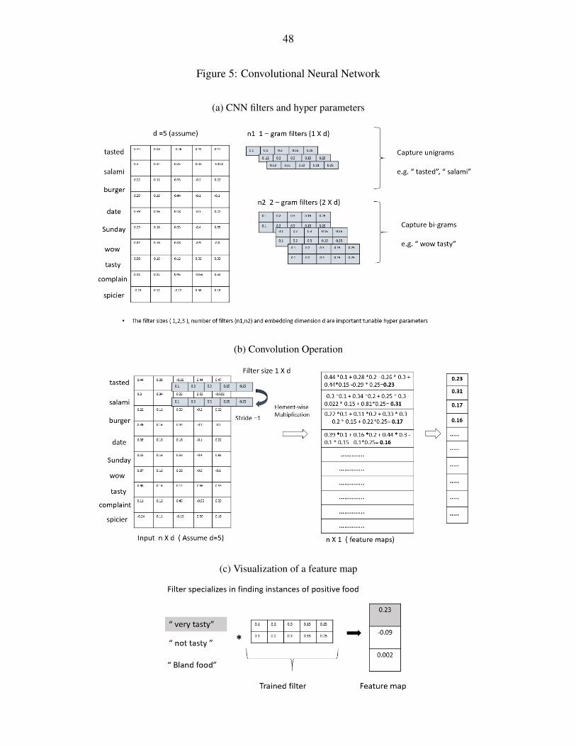
48

Figure 5: Convolutional Neural Network

(a) CNN filters and hyper parameters

(b) Convolution Operation

(c) Visualization of a feature map

49

Figure 6: Comparison of RNN and LSTM cells

(a) RNN cell

(b) LSTM cell

(c) Unrolled RNN and LSTM networks

50

Figure 7: Distribution of sentence length (number of words)

Figure 8: Illustration: Imputation for Missing Attribute Sentiment Scores

x

f (x)N(β 4

k , σ4k )N(β M

k , σMk )

A

N(β 3k , σ

3k )

x

f (x)N(β 4

k , σ4k )N(β M

k , σMk )

B

N(β 3k , σ

3k )

Note. Probability of score 3: AA+B , Probability of score 4: B

A+B

51

Figure 9: Text Mining Performance Evaluation Framework

Figure 10: Accuracy as a function of training data size and no of training cycles

(a) Training Data size (b) Training time (epochs)

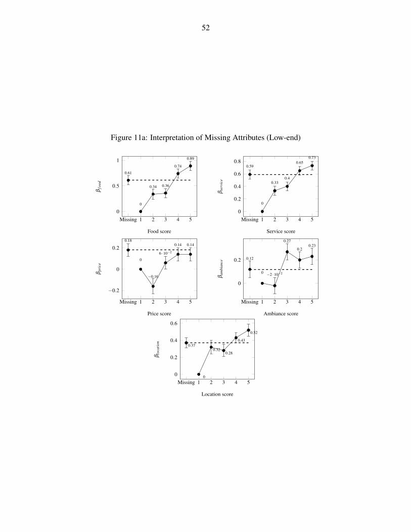
52

Figure 11a: Interpretation of Missing Attributes (Low-end)

Missing 1 2 3 4 50

0.5

1

0

0.34 0.36

0.74

0.89

0.61

Food score

βfo

od

Missing 1 2 3 4 50

0.2

0.4

0.6

0.8

0

0.330.4

0.650.73

0.59

Service score

βse

rvic

e

Missing 1 2 3 4 5

−0.2

0

0.2

0

−0.16

6 ·10−2

0.14 0.140.18

Price score

βpr

ice

Missing 1 2 3 4 5

0

0.2

0 −2 ·10−2

0.27

0.20.23

0.12

Ambiance score

βam

bian

ce

Missing 1 2 3 4 50

0.2

0.4

0.6

0

0.320.28

0.43

0.52

0.37

Location score

βlo

cati

on

53

Figure 11b: Interpretation of Missing Attributes (High-end)

Missing 1 2 3 4 50

1

2

3

0

1.591.88

2.3 2.432.13

Food score

βfo

od

Missing 1 2 3 4 50

0.5

1

0

0.41

0.6

0.81

0.95

0.7

Service score

βse

rvic

eMissing 1 2 3 4 5

0

0.2

0.4

0

9 ·10−29 ·10−2

0.19

0.25

0.18

Price score

βpr

ice

Missing 2 3 4 5

0

0.5

0−9 ·10−2

1 ·10−2

0.17

0.31

2 ·10−2

Ambiance score

βam

bian

ce

Missing 1 2 3 4 50

0.5

1

0

0.36

0.93

0.610.50.49

Location score

βlo

cati

on

Figure 12: Change in Proportion of Satisfied Customers (> 3 Stars) Left: low-end, Right: high-end

Food Service Price Ambiance Location

60

80

94.1

70.9

78.2

83.7

78.8

94.2

85

89.4

56

46

Attribute

Prop

ortio

n(%

)

Not corrected Corrected

Food Service Price Ambiance Location

60

80

100 96.3

80.3

72.9

80.983.3

95

81.1

65.7

77.1

71.2

Attribute

Prop

ortio

n(%

)

Not corrected Corrected