Asymmetric Effects on Risks of Virtual Financial Assets ... · which is based on information...

QFE, 2(4): 860–883. DOI: 10.3934/QFE.2018.4.860 Received: 12 November 2018 Accepted: 20 November 2018 Published: 22 November 2018

http://www.aimspress.com/journal/QFE

Research article

Asymmetric Effects on Risks of Virtual Financial Assets (VFAs) in

different regimes: A Case of Bitcoin

Zhenghui Li1, Hao Dong2, Zhehao Huang1*and Pierre Failler3

1 Guangzhou International Institute of Finance and Guangzhou University, Guangzhou, P.R.China 2 School of Economics and Statistics, Guangzhou University, Guangzhou, P.R.China 3 Department of Economics and Finance, Portsmouth Business School, University of Portsmouth,

Portsmouth, P01 3DE, UK

* Correspondence: Email: [email protected]; Tel: +02026097393.

Abstract: The rapid development of VFAs allows investors to diversify their choices of investment products. In this paper, we measure the return risk of VFAs based on GARCH-type model. By establishing a Markov regime-switching Regression (MSR) Model, we explore the asymmetric effects of speculation, investor attention, and market interoperability on return risks in different risk regimes of VFAs. The results show that the influences of speculation and investor attention on the risks of VFAs are significantly positive at all regimes, while market interoperability only admits a positive impact on risk under high risk regime. All of the three factors exert asymmetric effects on risks in different regimes. Further study presents that the risk regime-switching also shows asymmetric characteristic but the medium risk regime is more stable than any others. Therefore, transactions of investors and arbitrageurs are monitored by certain policies, such as limiting the number of transactions or restricting the trading amount at high risk regime. However, when return risk is low, it will return to a medium level if we encourage investors to access.

Keywords: asymmetric effect; market risk; Virtual Financial Assets; Bitcoin; Markov regime switching model

JEL codes: C32, C44, C51

1. Introduction

mailto:[email protected]

861

Quantitative Finance and Economics Volume 2, Issue 4, 860–883.

VFAs market has attracted widespread attention from the media and investors alike since 2008, which is based on information technology infrastructure for maintaining an accounting ledger while replying the processing transactions on the lack of central authority (Glaser et al. 2014). Bitcoin is the most popular VFAs around the world which accounts for 54% of total VFAs market (Coinmarketcap.com accessed on Oct 30th, 2018).

The VFAs volatility are quite different form traditional financial assets (Sapuric and Kokkinaki, 2014; Kristoufek, 2015; Osterrieder and Lorenz, 2017). On the one hand, from the internal perspective of VFAs, the imperfections of trading platform technology, the difference between VFAs and traditional financial assets in transaction costs and trading mechanisms make the risk of VFAs increase (Cocco and Marchesi, 2016; Groshoff, 2014; Carrick, 2016; Blau, 2017; Gkillas and Katsiampa, 2018). On the other hand, from the perspective of the external environment, the difficulty of policy supervision and the complexity of capital flows make VFAs risks more dynamic (Jacobs, 2011; Grinberg, 2012; Lan et al., 2016).

Asymmetry effect characterizes the differences in the impact mechanisms of VFAs’ different return risk regimes. For example, speculators could react strongly in low risk regime while they are the weakest in medium risk regime and more active under the high risk regime because of their confidence and advantage in market information. Understanding the asymmetric effects on return risks of VFAs is crucial for investors and policymakers. Theoretically, higher return risk of VFAs leads to higher differences in price (Sornette et al., 2018), which might attract speculators and investors from around the world. This ultimately impacts the prices of VFAs. In practice, however, the reactions of speculators and investors to the risks of VFAs might be complex because of different goals among them. All of them might exert asymmetric features in different regimes.

One common feature of many related literatures, given the complexity of the VFAs market operation, is that they have all assumed that the effects of speculation, market interoperabiity and investor attention on the value and volatility of Bitcoin are symmetric. As a speculative asset, understanding the volume return relationship is essential to shedding light on potential implications for trading strategies. Balcilar et al. (2017) showed that volume cannot help predict the volatility of Bitcoin returns at any point of the conditional distribution. Moreover, Blau (2017) did not find that, during 2013, speculative trading contributed to the unprecedented rise and subsequent crash in Bitcoin’s value nor did they find that speculative trading is directly associated with Bitcoin’s unusual level of volatility. Thus, in the Bitcoin trading platform, the effects of speculation on the price volatility should be asymmetric. This results in the fluctuation of trust from users and their acceptability to Bitcoin, which makes volatility of Bitcoin price constantly and drastically. Due to the drastic volatility of price, the coming problem is that speculators get speculative profits by using Bitcoin (Yermack, 2013; Luther, 2016).

Market interoperability can be defined as “the ability of the transfer of assets abroad at two or more different market unit”. VFAs provide a new channel for capital flow that can be untraceable. Such cash flows show the functions that VFAs can be considered as production factors (Li et al., 2017). Bitcoin has strong hedging effect with commodity futures and global uncertainty index, so it provides investors with enough arbitrage opportunities (Bouri, 2017a, 2017b; Lukáš, 2017). As VFAs transactions are anonymous, irrevocable and low-cost. It is convenient for criminals to transfer illicit money across the different markets under the supervision vacuum. The ECB (2012) report warns of the potential risks that criminals, fraudsters and money launderers could perform illegal activities via Bitcoin. Plassaras (2013) further proposed that Bitcoin should be regulated by the International Monetary Fund ensuring globally financial stability based on Article IV of the Articles of Agreement.

862


Pilkington (2013) provided an example telling that the Polish government froze the bank account of a Poland-based Bitcoin exchange, after a German bank had shown that several compromised accounts transferred stolen money without identification to it. Since 2005, China has experienced an acceleration of capital flight reaching $425 billion (plus/ minus $60 billion) in 2014 (Gunter, 2017). Thus the market interoperability as the channel of capital flight might be an important factor.

Investor attention is a scarce resource. When there are many alternatives, options that attract attention are more likely to be considered and hence more likely to be chosen, while options that do not attract attention are often ignored. Investor attention is mainly measured by psychological variables. Psychological studies on financial market have indicated that psychological variables produce a large influences on determining market prices (De, 1995). One big influence on people’s attitudes toward financial assets is the news and how financial assets are being perceived by the public because of the news (Andersen and Bollerslev, 1997). Kristoufeck (2013) and Glaser et al. (2014) found that internet (Google) searches determine the price of Bitcoin. Garcia et al. (2014) extended these results by showing that word-of-mouth information on social media and information on both Google Trends and new Bitcoin users have a significant influence on Bitcoin price changes. The authors also argued that the cost of Bitcoin production via mining represents a lower bound for Bitcoin price. A similar finding has been shown by Hayes (2016). Although speculation, investor attention and market interoperability are usually considered as important factors for understanding the risks of VFAs, there is no empirical investigation for the asymmetric effects on return risks of VFAs. Thus in this paper, we would explore the asymmetric effects through the MSR model.

We aim to contribute to the existing literature by showing the asymmetric effects of speculation, investor attention and market interoperability on return risks under different VFAs risk regimes. It is more reasonable to take the differences of regimes in VFAs market operation into account, which could be conducive to the market participants to make an efficient financial decision. The recent emergence of MSR model shows that allowing coefficients to switch between different regimes may provide a more realistic depiction of the driving the risks of VFAs forces. Hence, we provide evidence that the asymmetric effects under different regimes through estimating a MSR Model. Furthermore, analyzing on different impact factors can reasonably explain the dramatic fluctuations that occurring in the VFAs market at the beginning of 2013. It is likely that the factors dominating the VFAs market at different regimes might be different. We empirically investigate that the significant effects of market interoperability take place in a relatively high risk regime and other regimes with no effect.

On the data level, this paper considers China as a research object. On the one hand, Chinese government has closed the Initial Coin Offering (ICO) in China in October 2017 to prevent foreign exchange losses and control financial stability, but as a short-lived asset traded in China financial market, VFAs provides us with an invaluable dataset for the statistical research on trader’s behavioral charatics in China financial market. On the other hand, the people’s bank of China pays attention to develop the digital currency based on blockchain. Blockchains, the technology underpinning VFAs, are an instance of institutional evolution and sparked a new wave of innovation, which may start to revolutionize entreprene -urship and innovation (Davidson, 2018; Chen, 2018). Therefore, it is great significant to explore the asymmetric effect of VFAs’ return risk in different regimes in China market.

The analysis makes several significant contributions to the existing literature. First, while many studies have been works investigating the risk of VFAs, we compare different methods through loss functions and exam a better method to forecast the return risk of VFAs. Second, as noted, unliking

863


existing studies, the MSR Model can reasonable refer to the differences of regimes in VFAs market. This ensures accurate estimation and a better understanding the asymmetric effect in different regimes of VFA’s return risk. Third, we study influencing factors from different aspects. Because of VFAs’ decentralization and global, we think the main factor are speculative, market interaction and inventor attention. By analyzing the impact of these three aspects on different regimes risks, we can more comprehensively analyze the causes of the fluctuation of international VFAs prices.

The paper is organized as follows. The next section proposes some hypothesizes on the theoretical analysis for impact mechanism between risks of VFAs and speculative, market interaction and inventor attention. Then introduce the methodology used in this section. In Section 3, we expound the measurement of variables. In Section 4, we show the measurement results of return risk. In Section 5, empirical analysis on Bitcoin is carried out. Conclusions are given in Section 6.

2. The hypothesis and model

2.1. Hypothesis

Speculation is the most important factor affecting VFAs returns risk. Information is a key element of financial stabability (Mertzanis, 2018). Speculation can be regarded as informed trading, which is different from stock market (Feng, 2018). The decentralization of VFAs has caused a large amount of speculative capital to flow into the market continuously. These capitals increase the risk of the VFAs by affecting market liquidity, capital structure, and hedging. First, the entry of speculative capital has greatly increased the liquidity of the VFAs market, thereby attracting more diversified investors to enter the market, which further improves the market liquidity to some extent. Secondly, the speculators are supported by strong financial capitals. In addition, due to their keen sense diverse operations, they have gradually been the leading players in future market prices. What’s more, speculators admit keen senses of market. Thus information in the future market spreads very quickly and it is fully realized. In addition, electronic trading approaches are currently employed. Future market participants can quickly respond to subtle changes in market prices and efficiently avoid risks.

More and more investors are paying attention to the VFAs because of the involvement of speculators. From the theory of behavioral finance, it can be known that investors tend to show attention-driven trading behaviors and overconfidence tendencies. The more investors pay attention to the VFAs, the more likely they conduct trading activities. Overconfidence of investors might lead them to believe that their judgments on information are more accurate than others and that they could find potential information from published information. Therefore, they might think that they are more able than others to predict the direction of the VFAs market and assess the values of VFAs. The illusion of overconfidence in control is also a factor that leads to excessive trading. People often believe that they could affect the outcome of uncontrollable events and they are more convinced because of the increase in attention to information. As the interests of investors increase, more and more investment data are available, making them feel that they could better control the results of investments, thereby increasing the frequency of transactions.

Due to the borderless transactions of VFAs, market interoperability would be another important factor of return risk in the VFAs market. Most of them trading around the world originate from China and United States. Thus the difference between the market prices of China and United States is the main factor causing the fluctuation of risks in the VFAs market as well as the exchange rate between

864


RMB and U.S. dollar. Because of anonymity and lack of central authority, when compared with traditional financial assets, this supplies an opportunity to hedge with other markets causing the capital flight. From a macro viewpoint, abnormal capital flows have enhanced the difficulty to regulate foreign exchange and imposed higher requirements on maintaining the balance of international payments. Therefore, the market interoperability is an important factor affecting the stability of the virtual financial system. From the microscopic viewpoint, abnormal capital flows make the capitals outflow. This might easily result in the phenomenon that some investors are difficult to get out of the market, which violates the legitimate rights of investors and further makes the market unstable.

Accordingly, the following hypothesis is forwarded: H1: The factors impacting the risks of VFAs are speculation, investor attention and market

interoperability. The influence factors show different in different risk regimes. In the low risk regime,

speculation is a main factor. Speculators could usually obtain VFAs market information earlier such that they could make better judgments on the stability of the market. With a large amount of speculative capitals entering the VFAs market, the structure of funds in the market has been changed. It has attracted the attention of some investors. At this time, individual investor has begun to enter the VFAs market. However, speculative capitals in the market still occupy a large majority. Since speculators only pay attention to expected returns and obtain information in advance, speculators would generally withdraw early before major fluctuations of VFAs market occur. The withdrawal of large amounts of funds could easily cause market panic and further increase market risks.

With the risks increasing, investor attention plays a major role in the risks of VFAs market. Since the risk level is still within the range of some speculators, most speculators have already left the VFAs market (Murad, 2016). As VFAs market prices are gradually stable, individual investor began to enter the market. Due to the ineffectiveness of the VFAs market and the "herd effect" of investors, investors began to follow suit, making the prices increase more. When the VFAs market price exceeds the expectations of investors, there appears a phenomenon selling VFAs, which also leads to a fall of VFAs price. Since the entire process is dominated by the follow up transactions of investors, VFAs prices fluctuate more violently and VFAs market stability would decrease. As a result, market risks have increased significantly.

In high risk regime, market interoperability begins to work on VFAs return risks. Risk-biased investors prefer that turbulence in earnings is better than the stable earnings and that incomes brought by the assets exceed their expectations. Therefore, investor attention is still the main factor at this time. The borderless nature of VFAs transactions allows more arbitrageurs to enter the VFAs market. Arbitrageurs are more sensitive compared with speculators. They can realize the difference of VFAs prices in difference markets and then quickly draw up corresponding trading strategies. In the VFAs market, the arbitrage target is mostly achieving the transfer of funds. Thus the large amount of capital changes would make the VFAs market less stable, which in turn increases the risks of VFAs market. However, due to the government policies, the linkage among the markets is not the most important factor in the market risks.

Accordingly, the following hypothesis is forwarded: H2: The influence factors are different in different risk regimes. Speculation and investor

attention are main factors. Market interoperability causes high risks. Speculators and investors influence the return risks of VFAs differently. The impact of

865


speculation on the risks of VFAs was “U-shaped” and the one of investor attention showed a linear increasing trend. Under the low risk regime, since speculators admit certain advantages in obtaining information, they grasp the market better and could better judge the current status of the market. As a result, speculators enhance the risks of VFAs through manipulating the market. At this time, investors cannot understand the market enough and impact a little on market risks. As the risks of VFAs increase, speculators begin to withdraw from the market. As the profits of investors lead to the expansion of the “herd effect” in the market, a large number of investors enter the market. Therefore the speculative effects on the risks of the VFAs are the smallest but investor attention on the market risks increases. Under the high risk regime, speculators who admit partial risk appetites are confident on their own operations due to the convenience of market information acquisition. Hence speculators have begun to enter the market. However, due to the high risk regime at this time, the number of speculators in the market would be less than the one in the low risk regime but higher than the one in the medium risk regime. Thus the market risks impacted via speculative effects would increase compared with the one in the medium risk regime. At the same time, due to the manipulation of speculators, market volatility becomes more drastic. The probability of investors gaining profits would increase such that the “herd effect” would further increase. Therefore, investor attention has a greater impact on market risks.

Market interoperability shows asymmetric effects on the return risks of VFAs. Market interoperability mainly refers to arbitrage and money laundering due to different prices in different markets. Since the price volatility of the VFAs is small under the low and medium risk regimes, the profits of the arbitrageurs are small. Hence the arbitrageurs would not choose this way to realize their own profits. In the high risk regime, the fluctuant prices of the VFAs are fierce. The spread among the markets increases as well and the arbitrageurs begin to enter the market. Therefore, in the low and medium risk regime, the interactions among markets might not significantly impact on market risks, while the high risk regime plays a significant role in promoting market risk.

Accordingly, the following hypothesis is forwarded: H3: All of speculation, investor attention and market interoperability exert asymmetric features

in different regimes.

2.2. The model

From the hypothesis analysis, we can know that the factors impacting the risks of VFAs are speculation, investor attention and market interoperability. What’s more, these influence facors are regime-dependent. Therefore we consider establishing MSR Model (Hamilton, 2008). In addition, the application of the MSR Model is mainly based on the following reasons. Firstly, the model need not artificially set thresholds to determine different regime levels of risks, nor does it need to estimate in advance the timing of each regime system. Instead, the risk level is determined by smooth transition among state variables in different risk regimes. The parameters of the maximum likelihood estimation model can be used to obtain specific time for different regimes. It is logical to interpret the differences of the influence factors under different risk regimes through MSR model. Secondly, the MSR Model reflects the dynamics of the transition among different risk regimes through state transition variables.

The MSR Model is written as (1).

866


( )( ) ( )( ) ( )( ) ( )( ) ( )( )1 2 3 .Risk c S t S t spe S t igz S t iex S tβ β β ε= + + + + (1)

where ( )S t is an unobservable variable governed by a first order Markov process. Variable spe

represents the speculation of Bitcoin market, igz stands for the investor attention and iex is the

market interoperability between China and the United States. Function ( )( )i S tβ is the impact

degree of factor i on state ( )S t .

Under certain conditions, state transition of the risk of Bitcoin is achieved by the transition

probability uvp , namely that the probability from state u at time 1t − to state v at time t . It can

be expressed as (2).

( )1Pr .uv t tp S v S u−= = = (2)

It also satisfies that (3).

1, 1,2, , , 1.v M

uvvu v M p=

=∀ = =∑ (3)

3. The measurement of variables

3.1. Dependent variables

The Value-at-Risk (VaR) or Conditional VaR (CVaR) reflects the maximum amount of loss exposed in Bitcoin during a specific holding period. It could be considered as a vital tool to demonstrate the risk level before starting the risk management. When calculating the VaR (CVaR), authors usually employed the non-parametric method and parametric method. The historical simulation method is a non-parametric method. It requires too much old information contained in the data. Since the prices of Bitcoin are not limited, the information could not accurately describe the future situation. In addition, we focus on the fundamental situation in the market of VFAs in this paper. Thus we measure the risk level of Bitcoin through a paramet -ric method. The calculating procedure is given as follows. Firstly, we put forward a new measurement method to calculate the Bitcoin return. Secondly, we capture the volatility based on a GARCH-type model. Finally, we measure the VaR and CVaR of the Bitcoin market.

Bitcoin transactions are between speculative investors, and only minorities are used for purchases of goods and services (Yermack, 2015; Baur et al., 2017). Due to the Globalization and decentralization of Bitcoin, the returns are achieved by two separate sources: arbitrage trades and speculative trades from investors. Returns from arbitrage trades are dependent on jet lags in different markets. The arbitragers focus on the differences among different Bitcoin markets. In addition, the trading volume would be large. Thus there might be a deviation of the return rate if using the closing prices published on the web site. When speculative trades happened, the changes of price reflect the expectation of informed investors on the future payoffs of Bitcoin. Since the information is

867


asymmetry and the price is unlimited, the Bitcoin price might suffer a sudden change of vibration frequency and amplitude. The closing price, however, could only be seen as the price of Bitcoin at the closing time and cannot reflect the volatilities of Bitcoin intraday price. What’s more, average quoted implies that Bitcoin is investible (Dyhrberg, 2018). Thereby, we put forward an average for the intraday price of Bitcoin and take the highest and lowest intraday prices into consideration. The result is given as (4).

.2

t tt

ph plrp += (4)

where trp is the intraday price at time t , tph is the highest intraday price at time t and tpl is the lowest intraday price at time t . According to (4), we describe the return through the logarithmic difference of the Bitcoin intraday daily price as (5).

1ln ln .t t tr rp rp −= − (5)

where tr represents the return sequence of the Bitcoin intraday price. For the volatility measurement, authors usually employed the following two methods: stochastic

volatility (SV) model and generalized autoregressive conditional heteroscedasticity (GARCH) model. The main difference between these two models is the hypothesis on the residual term. The SV model assumes that the residual term in the autoregressive process of the Bitcion return is a stochastic process. Due to the convenience of Bitcoin such as lower transition cost, the price volatility is mainly driven by the expectations of investors on the future payoffs of Bitcoin. In addition, there are many speculators and arbitragers being the sources of “herd effect” due to lack of regulation in Bitcoin market. Thus the volatility is time-varying, i.e. heteroscedasticity effect. Therefore, we estimate the volatility of the Bitcoin return sequence through the GARCH model (Bollerslev, 1986).

The basic structure of the GARCH model can be written as (6) and (7).

.t t t tr µ σ ε= + (6)

.1

21

20

2 ∑∑ = −= − ++=p

j jtjq

i itit σβεαασ (7)

where (6) is the mean value equation of Bitcoin return series. We establish AR model by using the return sequence to filter out the lag correlation in the return sequence. (7) is the conditional

variance equation of Bitcoin return series. tσ describes the agglomeration effect of the return

sequence of Bitcoin. Although widely used in practice, the GARCH model does not account for the leverage effect

which is the fact that negative shock tends to produce different volatility compared with positive ones. It is assumed in the GARCH model that only the magnitude of investor expectations determines the feature volatility of Bitcoin rather the positivity or negativity shock. In addition, if the shocks on volatility persist indefinitely, the entire term structure of Bitcoin risk might be moved resulting in a significant impact on the investment of Bitcoin. Thus, in order to depict the volatility of the Bitcoin price more accurately, we apply the EGARCH model proposed by Nelson (1991).

The mean equation of the EGARCH model is captured by (6) but the conditional variance

868


equation is given as (8).

2 20

1 1 1ln ln .

q p rt i t i t k

t j t j i kj i kt i t i t k

Eε ε εσ α β σ α γ

σ σ σ− − −

−= = =− − −

= + + − +

∑ ∑ ∑ (8)

In (8), the statistically significant and negative coefficient γ indicates the presence of leverage

effect. Leverage effect refers to the phenomenon that negative shock leads to higher volatility than

positive shock of the same magnitude. jβ measures the persistence of volatility shock.

For VaR measure, we assume that the residual series of Bitcoin return in (6) obeys the GED distribution. It has been proved that the result is also suitable for other GARCH-type models. From the above analysis, the variance equation can be expressed as (9) and (10).

( )2 21

~ 0, , ,t ttR GEDε ν σ

− (9)

.21

210

2−− ++= ttt βσαεαδ (10)

In (9), ( )20, , tGED ν σ is a GED distribution with a zero mean value, a degree of freedom v and a

variance 2tσ . According to (10), we can calculate the standard deviation tσ via the GARCH model

and furthermore calculate the VaR in Bitcoin market as (11).

1 .t t tVaR rp ασ−= (11)

where tVaR stands the Bitcoin risk at time t . And α is a quantile given the confidence level c

(Cabedo and Moyab, 2003). CVaR is an extension of VaR and defined as the average loss over a certain threshold. For

Bitcoin return series tr with distribution function g , the CVaR of tr at confidence level

100(1-c)% can be defined as (12).

( ) ( ) .CVaR E g r g r VaR = > (12)

It is easily known from (12) that CVaR is expected to be an extreme value greater thanVaR . After we get the VaR of certain confidence level and distribution hypothesis, we can get the CVaR by calculating the corresponding conditional expectation (Rockafellar, 2002). Thus (12) is further expressed as (13).

1 1 1[ ].t t t t t t tCVaR E rp q rp q rpσ σ ασ− − −= > (13)

869


In (13), q represents the quantile greater than α .

Let ( )f q be the probability density function of the corresponding distribution, then (13) can be

reduced to be (14).

1 ( ) .1

t tt

pCVaR qf q dqc α

σ +∞−=− ∫ (14)

3.2. Explanatory variables

The explanatory variables include speculation, investor attention and market interoperability. According to Part 2, the first driver of exchange rate risk is speculation. Bitcoin return and volumes are associated with speculation. When measuring speculation, we follow the work of Llorente et al. (2002) and use a time series model that identifies the dynamic relation between return and volume. We estimate daily turnover of day t as (15) and (16).

log log( 0.00000255).t tturn turn= + (15)

1

50

1log log .50t t t ss

v turn turn−−=−

= − ∑ (16)

where tturn is the trading volume of Bitcoin in day t and tv stands for the (50 day) detrended

measure of trading activity. Thus we measure the speculation as (17).

.t t tspe r v= × (17)

where tr is the daily return of Bitcoin in day t .

Investor attention is measured from the demand side. In general, Bitcoin could be seen as a standard good whose risk is influenced by demand and supply. In the supply side, the number of Bitcoin is fixed. This makes little contribution to the risk. The demand side in the Bitcoin market is driven only by expected profits holding the currencies and selling them later. Thus the market is dominated by short-term investors, trend chasers, noise traders and speculators. Google Trends counts the searching amount of the key word “Bitcoin” over a period and investigates the popular extent in the current period. Therefore the searching frequency of terms related to Bitcoin could be considered as a good measure for investor attention through Google Trends. Hence we measure the investor attention through Google Trends.

The Bitcoin-implied exchange rate among different markets is an important manifestation for market interoperability. Following the work of Lan et al. (2016), we define the Bitcoin-implied exchange rate as (18).

.RMB

im tUSDt

BEB

= (18)

870


where RMBtB stands for the market price in RMB and USD

tB the market price in USD. Most of

Bitcoin trades in the world occurs in these two markets. As the open market RMB/USD exchange rate should apply and the transaction is transparent and traceable, if the market is efficient, the difference between the Bitcoin-implied exchange rate and the open market exchange rate is little. Thus we define the market interoperability as (19).

.im op

op

E EiexE−

= (19)

where opE is the open market exchange rate. Hence, if the market is fully communicating, iexshould not be statistically different from zero.

4. The results of risk measurement

Considering the early issuance of Bitcoin, the price volatility is relatively small, especially compared with the current price of Bitcoin. This might cause some extreme impacts on data analysis. In addition, Bitcoin price went through a strong volatility in 2013. Chinese central bank issued the regulatory policy on guarding against the risk of Bitcoin strengthening the supervision of Bitcoin. Thus we select the related data of intraday Bitcoin transactions in Chinese market from January 1, 2013 to May 31, 2017. All the data are picked up from Bitcoin data website (https: //bitcoincharts.com/).

Following (11), we need to determine the α for each distribution, such as normal, student t and

GED distribution, at a confidence level 100(1-c) % before calculating the tVaR and tCVaR . The

quantiles are obtained with different distributions. The results are shown in Table 1.

Table 1. The quantiles of the model under three different distributions.

Distribution Freedom c Quantile GARCH-N 0.10 1.282

0.05 1.645

GARCH-T 2.911621 0.10 1.651254 0.05 2.382773

GARCH-GED 0.913168 0.10 1.107681 0.05 1.613537

EGARCH-N 0.10 1.282 0.05 1.645

EGARCH-T 2.898603 0.10 1.653330 0.05 2.387307

EGARCH-GED 0.908783 0.10 1.105980 0.05 1.612643

Table 2 shows the descriptive statistics on the VaR series. We can see that under the confidence level of 0.1, the VaR series based on the EGARCH-T distribution show the most violent volatility with the largest average daily loss of ¥226.96. The VaR series based on the GARCH-GED distribution show the least volatility and the average daily loss is the smallest ¥125.09. The volatilities of VaR series based on GARCH-N distribution are stronger than the ones based on the GARCH-GED distribution. However, the average daily loss is ¥142.64, which is larger than the latter ¥125.09. At the confidence level of 0.05, the

871


most volatile ones are still the VaR series under the EGARCH-T distribution with an average daily loss of ¥327.73. The least volatile ones are the VaR series under the GARCH-N distribution.

Table 2. Descriptive statistics on VaR series.

Confidence level

Model Mean Maximum Minimum St.dev Q

0.10 GARCH-N 142.6426 1745.7899 1.685461 180.34787 222342.18 GARCH-T 213.2395 3007.4725 1.462772 312.64463 322267.74 GARCH-GED 125.0951 1684.9371 0.981892 176.72301 200042.54 EGARCH-N 147.6072 6059.0033 0.713601 239.70521 229382.95 EGARCH-T 226.9696 21353.7197 0.728903 673.57114 344634.17 EGARCH-GED 129.1716 8383.8640 0.484985 289.30224 208255.76

0.05 GARCH-N 183.0319 2240.1126 2.162701 231.413612 283516.56 GARCH-T 307.7063 4339.8067 2.110791 451.148679 476637.13 GARCH-GED 182.2234 2454.4144 1.430303 257.428899 282264.17 EGARCH-N 189.4024 7774.6181 0.915659 307.578054 293384.31 EGARCH-T 327.7301 30833.4634 1.052491 972.595483 507653.98 EGARCH-GED 188.3466 12224.6087 0.707163 421.834935 291748.94

The last column of the table 2 represents the value of the loss function. The loss function used in this paper is given as (19).

( )1

.n

t t tt

Q VaR CVaR sy=

= −∑ (19)

( )t tVaR CVaR are the measurement results of Bitcoin return risk in day t . tsy is the profit or loss in

day t . It is calculated as (20).

1.t t tsy rp rp −= − (20)

We clearly notice that under the confidence level 0.1, the Q value of the T distribution is the largest and the one of the GED distribution is the smallest. It can be seen that the fitting results based on the GED distribution are the most optimal followed by the normal distribution. The results of T distribution are the worst. The same results can be obtained from Figure 1 and Figure 2 as well.

Figure 1 and Figure 2 show the Bitcoin return risk during the sample period. It can be seen from Figure 1 and Figure 2 that the VaR based on the T distribution admits a higher outlier in mid-2016. This leads to the reduction of the measuring effect. In addition, in the initial stage of Bitcoin issuance, the risk was relatively small and stable. At the end of 2013, due to the emergence of Internet Finance, Bitcoin went into the eyes of investors. As a result, the Bitcoin price had risen up and as well as the risk. The increased risk level has aroused the concern of regulators. Therefore, in December 2013, Chinese central bank issued the regulatory policy coping with the Bitcoin risk and achieved significant results in decreasing the risk of Bitcoin. However, with the increase of investors at this time, the risk returned to the initial level just until the end of 2015. After a year of smooth transition,

872


Bitcoin was not regulated as desired but showed a rising trend. The risk showed an upward trend as well.

Figure 1. VaR series under the confidence level of 90%.

Figure 2. VaR series under the confidence level of 95%.

Since VaR cannot accurately reflect the losses caused by extreme events, and it does not satisfy the consistency and additivity, in this paper, we further calculate the CVaR based on the GARCH-type model. The results are shown in Table 3.

Table 3 shows the descriptive statistics on CVaR series. We can see that the CVaR series based on different distributions volatilize more strongly regardless of the confidence level 0.1 or 0.05. The CVaR series based on the EGARCH-T distribution are the most violent at the confidence level 0.1 with the standard deviation given as 1213.492 and the average extreme loss ¥408.9. The CVaR series based on GARCH-N are the least violent. The standard deviation is 246.744 and the average extreme loss is ¥195.16. At the confidence level 0.05, the CVaR series based on the EGARCH-T distribution are still the most volatile with the standard deviation 1624.29 and the average extreme loss ¥547.32. The CVaR series based on the GARCH-N distribution admit the least average loss, which is ¥229.45. The corresponding volatility is the most moderate and the standard deviation is 290.11.

873


Table 3. Descriptive statistics on CVaR series.

Confidence level Model Mean Maximum Minimum St.dev Q 0.10 GARCH-N 195.1572 2388.501 2.306039 246.7439 295613.5

GARCH-T 383.4714 5408.396 2.630541 562.2332 582355.1 GARCH-GED 208.9249 2814.067 1.63989 295.15 315528.4 EGARCH-N 201.9495 8289.658 0.976325 327.954 306241.6 EGARCH-T 408.9036 38470.41 1.31327 1213.492 621880.3 EGARCH-GED 208.9441 2814.325 1.640041 295.1771 315557.2

0.05 GARCH-N 229.4539 2808.253 2.711299 290.1063 346533.9 GARCH-T 512.8995 7233.821 3.518393 751.9964 781872.2 GARCH-GED 267.575 3604.041 2.100246 378.0055 404390 EGARCH-N 237.4399 9746.472 1.147903 385.5883 358890.1 EGARCH-T 547.3266 51493.5 1.757841 1624.286 835460.7 EGARCH-GED 267.7737 3606.718 2.101806 378.2863 404693

The last column of Table 3 shows the values of the loss function. We clearly notice that the value of the loss function of CVaR series based on the N distribution is the smallest at the confidence level 0.1 and 0.05. It can be seen that the measurement method through CVaR based on the normal distribution is more optimal than the other two distributions. Under the same level of confidence, the CVaR series based on GARCH-N are more optimal than those based on EGARCH-N. The same results can be obtained from Figure 3 and Figure 4.

Seeing from Figure 3 and Figure 4, the CVaR series under different distributions show significant differences. The CVaR series based on the T distribution is significantly higher than those based on the N distribution and GED distribution. In addition, from the values of the loss function, the CVaR series based on the GARCH-N model can well cover the loss series such that the Bitcoin return risk would not be overestimated.

According to the above analysis, we compare the VaR and CVaR series obtained from the GARCH model based on the N distribution. The comparison for some statistical propertyes is shown in Table 4.

Figure 3. CVaR series under the confidence level of 90%.

874


Figure 4. CVaR series under the confidence level of 95%.

Table 4. Comparison of VaR and CVaR series based on Normal Distribution of GARCH Model.

Confidence level VaR/CVaR Mean Maximum Minimum Q 0.1 VaR 142.6426 1745.7899 1.685461 222342.18

CVaR 195.1572 2388.501 2.306039 295613.5 0.05 VaR 183.0319 2240.1126 2.162701 283516.56

CVaR 229.4539 2808.253 2.711299 346533.9

Table 4 shows the difference between VaR and CVaR series based on Normal Distribution of GARCH Model. Under the same confidence levels, investors face more losses under extreme conditions than under normal conditions. The range of the investment loss is higher at any time. When the confidence level is 0.1, the maximum value of loss is ¥1745.79, the average loss is only ¥142.64 and the range is ¥1744.1. While under the extreme conditions, the maximum loss is ¥2388.5, the average loss is ¥195.16 and the range is ¥2386.19. At the confidence level 0.05, the difference between CVaR and VaR reduces. Under the extreme conditions, the biggest loss is ¥2808.25, the average loss is ¥229.45 and the range is ¥2805.54. Under normal circumstances, however, the average loss is ¥183.03 and the difference between the maximum loss and the minimum loss is ¥2237.95. It could be seen that the risk of Bitcoin shows an expansion trend. Besides, the possibility of market shocks experi -enced by investors also increases. Therefore, when making investment decisions on VFAs such as Bitcoin, investors need to consider their own risk preferences and make correct investment decisions. The government needs to put forward appropriate risk regulation policies protecting the legitimate rights of investors.

5. Empirical results

In this section, we firstly compare the differences among different factors and regimes by esti -mating a MSR Model. Secondly, based on the quantile of the Bitcoin risk distribution, we artificially set the values for different regime of risk and then test the robustness of the MSR Model. Finally, we further analyze the results of regime distribution and transition probability during the sample period.

875


For convenience, we pick up data from the following ways. In Section 4, it is known that the CVaR series obtained from the GARCH model based on the N distribution can well cover the loss series, thus the CVaR series could be regarded as the Bitcoin market risk. Other data originate from the Bitcoin data website (https://bitcoincharts.com/), Google website (http:// trends.google.com) and State Administration of Foreign Exchange (http://www.safe.gov.cn/).

5.1. Estimate for the MSR Model

Data preprocessing is a preparation before estimating the model. The data should be normalized making the speculation, investor attention and market interoperability comparable. In this paper, we apply the Z-score normalization method. Figure 5 shows the series after normalization. From Figure 5, we can see that the volatility of Bitcoin risk is roughly similar to the speculation, investor attention and market interoperability. When Bitcoin risk is high, the values of speculation, investor attention and market interoperability are all higher than the risk level. This tells that when the Bitcoin risk lies in a high level, the speculation, investor attention and market interoperability further amplify the risk. When the risk is low, the values of speculation, investor attention and market interoperability are low as well. Nevertheless, the values are still higher than the risk level. We claim that the speculation, investor attention and market interoperability are still promoting the risk.

Figure 5. The sequence diagram after normalization.

After solving the comparison of variables, we need to determine the regime number before estimating the model. In general, the regime number is determined by the AIC and SIC criteria. The results of AIC and BIC tests are shown in Table 5.

Table 5. The results of AIC and BIC tests.

Regime number AIC BIC LogLik 2 488.5896 583.5555 -236.2948 3 -133.9947 8.454157 78.99737

876


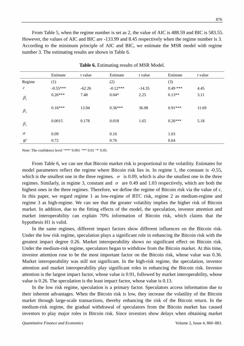
From Table 5, when the regime number is set as 2, the value of AIC is 488.59 and BIC is 583.55. However, the values of AIC and BIC are -133.99 and 8.45 respectively when the regime number is 3. According to the minimum principle of AIC and BIC, we estimate the MSR model with regime number 3. The estimating results are shown in Table 6.

Table 6. Estimating results of MSR Model.

Estimate t value Estimate t value Estimate t value Regime (1) (2) (3) c -0.55*** -62.26 -0.12*** -14.35 0.49 *** 4.45

1β 0.26*** 7.48 0.04* 2.25 0.13** 3.11

2β 0.16*** 13.94 0.36*** 36.08 0.91*** 11.69

3β 0.0015 0.178 0.018 1.65 0.26*** 5.18

σ 0.09 0.16 1.03 2R 0.72 0.76 0.64

Note: The confidence level ‘***’ 0.001 ‘**’ 0.01 ‘*’ 0.05.

From Table 6, we can see that Bitcoin market risk is proportional to the volatility. Estimates for model parameters reflect the regime where Bitcoin risk lies in. In regime 1, the constant is -0.55, which is the smallest one in the three regimes. σ is 0.09, which is also the smallest one in the three regimes. Similarly, in regime 3, constant and σ are 0.49 and 1.03 respectively, which are both the highest ones in the three regimes. Therefore, we define the regime of Bitcoin risk via the value of c. In this paper, we regard regime 1 as low-regime of BTC risk, regime 2 as medium-regime and regime 3 as high-regime. We can see that the greater volatility implies the higher risk of Bitcoin market. In addition, due to the fitting effects of the model, the speculation, investor attention and market interoperability can explain 70% information of Bitcoin risk, which claims that the hypothesis H1 is valid.

In the same regimes, different impact factors show different influences on the Bitcoin risk. Under the low risk regime, speculation plays a significant role in enhancing the Bitcoin risk with the greatest impact degree 0.26. Market interoperability shows no significant effect on Bitcoin risk. Under the medium-risk regime, speculators began to withdraw from the Bitcoin market. At this time, investor attention rose to be the most important factor on the Bitcoin risk, whose value was 0.36. Market interoperability was still not significant. In the high-risk regime, the speculation, investor attention and market interoperability play significant roles in enhancing the Bitcoin risk. Investor attention is the largest impact factor, whose value is 0.91, followed by market interoperability, whose value is 0.26. The speculation is the least impact factor, whose value is 0.13.

In the low risk regime, speculation is a primary factor. Speculators access information due to their inherent advantages. When the Bitcoin risk is low, they increase the volatility of the Bitcoin market through large-scale transactions, thereby enhancing the risk of the Bitcoin return. In the medium-risk regime, the gradual withdrawal of speculators from the Bitcoin market has caused investors to play major roles in Bitcoin risk. Since investors show delays when obtaining market

877


information, the responses to the market have time lags. Therefore, it has become the most important factor on Bitcoin risk to obtain information form internet at this regime. Under the high risk regime, investors blindly follow suit, making the volatility of Bitcoin price gradually increases. At this time, many arbitrageurs began to speculate on the differences of price among different Bitcoin markets, causing the “visual rise” phenomenon of Bitcoin price. Thus, investors are still the most important impact factor.

Under different regime, the same impact factors address different effects on Bitcoin risk. The impact of speculation on the Bitcoin risk was “U-shaped” (The values in low, median and high risk regimes are 0.26, 0.04 and 0.13 respectively). Due to the convenience of the speculators in obtaining the information, they are more accurate in leading the market. Under the low-risk regime, speculators hold a large amount of capitals to enter the Bitcoin market, impacting greatly on the market price. When reaching the expected profits of most speculators, only risk-seeking speculators play key roles in the Bitcoin market. Thus the speculation adder -sses the lowest impact on medium risk regime. As the risk level increases, the confidences of the speculators lead to the entries to the market of more risk-seeking speculators. They manipulate Bitcoin prices together with arbitrageurs and thereby enhance the Bitcoin risk.

The influence of investor attention on Bitcoin risk shows a linear increasing trend. Under the low-risk regime, the impact of the investor attention on Bitcoin risk is 0.16, while under the medium-risk regime, the impact on Bitcoin risk is 0.36. The one under high-risk regime is 0.91. This tells that Bitcoin risk is mainly caused by investors following the linear trend of trading. When the Bitcoin risk is low, the investors, with a wait-and-see attitude, are afraid to trade Bitcoin due to their lack of self-confidence and information on the market. With the development of Bitcoin, it is paid more and more attention. At this time, the volatility of the Bitcoin price has increased. The self-confidences of some investors have led them to start participating in market transactions. The increase of the risk implies the increase of Bitcoin price volatility. Some investors would experience “a day of riches” and are more confident. As a result, Bitcoin risk gradually increases.

Market interoperability addresses asymmetric effect on the Bitcoin risk. From Table 6, it is known that market interoperability is not significant on the Bitcoin risk under both the low and medium risk regimes. However in the high risk regime, the impact is 0.26. This shows that market interoperability provides opportunities for arbitragers. Arbitragers are more agile than speculators. They could realize the differences of Bitcoin price among the markets and then quickly come up with corresponding trading strategies. In the Bitcoin market, target of arbitragers is achieving the transfer of funds. This leads to the less stable Bitcoin market due to the large amount of capital changes, which in turn would increase the Bitcoin risk. In summary, the hypotheses H2 and H3 are valid.

5.2. Robustness Tests

In the last subsection, we verify the effectiveness of hypotheses H1, H2 and H3 through estimating the MSR Model and analyzing the parameters. In this subsection, we test the robustness of the model. The thresholds of different risk regimes are artificially determined according to the following criteria. Firstly, we ensure enough sample size to test the robustness of the model. Secondly, during the sample period, several peaks appeared in the Bitcoin risk and the extremely maximum values are different. Sufficient high quantiles might cause the loss of some maximum values, thereby affecting the results of robustness. Thirdly, the difference between the minimum and maximum values of Bitcoin risk during the

878


sample period is signifi -cant. The quantiles which are complementary to high-risk regime might ignore this difference. Therefore, it is impossible to better describe the robustness of the impact factors in the low risk regime. Thus we define two variables capturing days when Bitcoin return risk exceeds 90% (High regime) and is below 5% (Low regime). The residual data is considered as the Medium-risk regime. Finally we regard these variables as explained variables and estimate the regression for robustness tests. The results of robustness tests are shown in Table 7.

Table 7. Results of robustness tests.

Explained variable Low regime Medium regime High regime c -0.63 *** -0.17 *** 0.90***

1α ( spe ) 0.41 ** 0.02* 0.14**

2α ( igz ) 0.16*** 0.35*** 0.73***

3α ( iex ) -0.1 0.002 0.26***

2R 0.76 0.52 0.48

Note: The confidence level ‘***’ 0.001 ‘**’ 0.01 ‘*’ 0.05.

From Table 7, it can be seen that different impact factors show significant differences under the same regimes. Under the low risk regime, speculation addresses the largest impact on the Bitcoin risk, which is 0.41. Market interoperability shows no significant effect on Bitcoin risk. Under the medium-risk regime, investor attention addresses the greatest impact on the Bitcoin risk, which is 0.35. The effect of market interoperability on the Bitcoin risk is still insignificant. Under the high-risk regime, the speculation, investor attention and market interoperability play significant roles in enhancing the Bitcoin risk. The impact of investor attention on the Bitcoin risk continues to increase. It is still the most influential factor among the three factors, which is 0.73, followed by market interoperability, which is 0.26. The speculation addresses the least impact on the Bitcoin risk, which is 0.14.

Under different risk regimes, each impact factor addresses different effects on Bitcoin risk. The impact of speculation on the Bitcoin risk was “U-shaped” (It is 0.41 in the low-risk regime, 0.02 in the median risk regime and 0.14 in the high risk regime). The impact of investor attention on Bitcoin risk showed a linear increasing trend. Under the low-risk regime, the impact of investor attention on Bitcoin risk is 0.16, while under the medium-risk regime, the impact on Bitcoin risk is 0.35. The impact under the high-risk regime is 0.73. Market interoperability is not significant on the Bitcoin risk under the low or medium risk regime. However under the high risk regime, it admits a significant impact with 0.26.

In summary, through artificially determining different risk regimes, we explore the impact of Speculation, investor attention and market interoperability on the Bitcoin risk. The results are mostly the same as those obtained from the MSR Model, which implies that the results obtained from the MSR Model are robust.

879


5.3. Discussion

Figure 6 shows the Bitcoin return risk regimes during sample period. In Figure 6, (a) represents the low-risk regime, (b) stands for the medium-risk regime and (c) is the high-risk regime. We clearly notice that the Bitcoin risk mainly aggregated in the medium-risk regime. The low-risk mainly happened in the initial period of Bitcoin issuance. Policies have certain limits on the high risks. In the early days of Bitcoin issuance, investors were not paying much attention. At this time, speculative capital played major roles on the Bitcoin market. As a result, Bitcoin risk rose slightly. The government catched this phenomenon timely and made some regulation policies to hold-up the Bitcoin risk. Thus it dropped to a low risk regime. As investors entered the Bitcoin market, the Bitcoin risk fluctuated between medium and high levels. Due to the follow-up transactions in the Bitcoin market, Bitcoin risk gradually increased. At the same time, the remainder risk-seeking investors in the market continued contributing to the Bitcoin risk. Through the effective guidance of government policies, Bitcoin risk returned to a median level. The same result can be seen in Table 8.

Table 8 shows the transition probability of Bitcoin risk between two regimes. As it can be seen from the matrix, Bitcoin risk has a higher probability maintaining the current regime. Moreover, the higher risk regime, the more difficult to maintain it. The probability maintaining a low risk regime is 0.9689, the probability maintaining a medium regime is 0.9538 and the probability maintaining a high regime is 0.8575. This shows that under the low-risk regime, speculative capitals could better stabilize the operation of Bitcoin market. Under the medium-risk regime, the investor participation reduced the stability of the market. Under the high-risk regime, the arbitrage and investors follow-up transactions mostly impact on the stability of the Bitcoin market.

In addition, there is not jump regime of Bitcoin risk. The probability from low-risk regime to high-risk regime is 0.0004 and the probability from high-risk regime to low-risk regime is 0.0096. This tells that when the government formulates regulation policies to regulate Bitcoin risk, it should be moderate in adjustment and control and follow the rules of the market. Otherwise, it might easily lead to market turbulence and the policies might play opposite effects.

The medium-risk regime admits strong stability. The transition between two regimes show asymmetric effects. As it can be seen from Table 8, the probability of Bitcoin risk remaining in the medium-risk regime is 0.95, which is only 0.01 less than the one maintaining the low risk regime and 0.1 larger than the one maintaining the high risk regime. Thus, we claim that the medium-risk regime admits strong stability. In addition, the transition probability from medium to high risk regime is 0.03 and the one from high to medium risk regime is 0.13. The transition probability from medium to low risk regime is 0.01 and the one from low to medium risk is 0.03. These claim that the transition between two regimes show asymmetric effects. These also show that when the government regulates Bitcoin risk, it should not excessively pursue low risk level. In contrast, the risk should be controlled in the medium regime. When the risk is in the high regime, the transactions of investors and arbitrageurs should be monitored through certain policies, such as limiting the number of transactions and the trading volume. When the risk is low, the market risk could return to a medium level by encouraging investors to enter the market. This would reduce the number of speculators and protect the legitimate rights of investors.

880


(a)

(b)

(c)

Figure 6. Bitcoin risk regimes.

Table 8. Matrix of transition probability.

Low Medium High Low 0.9689 0.0108 0.0096

Medium 0.0307 0.9538 0.1329 High 0.0004 0.0354 0.8575

881


6. Conclusions

In this paper, we measure the Bitcoin return risk through application of the VaR and CVaR theory based on GARCH-type model in different distributions and explore the asymmetric effects of three impact factors, speculation, investor attention and market interoperability on the Bitcoin risk in different regimes via a MSR Model. Specific conclusions are as follows.

The CVaR series obtained from the GARCH model based on the N distribution can better capture the VFAs risk. Through the loss function, we could know that the CVaR series based on the GARCH model in normal distribution could well cover the loss series and would not be much higher than the loss series. Thus it would not cause overestimation of the Bitcoin return risks.

Speculation, investor attention and market interoperability exert asymmetric effects in different regimes. The impacts of speculation on the VFAs risks was “U-shaped”. The impact of investor attention on VFAs risks showed a linear increasing trend. The market interoperability is not significant on the VFAs risks under low and medium regimes. However in the high risk regime, it shows significant impacts. Therefore, the authorities could strengthen the supervision of the VFAs platforms improving the trading mechanism to prevent the occurrence of platform security incidents.

Under the same regimes, the impacts of speculation, investor attention and market interoperability on VFAs risks are different and the transitions between two VFAs risk regimes show asymmetric effects as well. Under the low risk regime, speculation palys a significant role in enhancing the VFAs risks. Under the medium risk regime, the most important factor on the VFAs risks was the investor attention. While, under the high risk regime, speculation, investor attention and market interoperability all play significant roles in enhancing the VFAs risks. The most prominent impact factor is the investor attention, followed by the market interoperability and then the speculation. In addition, the matrix of transition probability shows the strong stability of medium risk regime. The transitions between two regimes address asymmetric effects. The transactions of investors and arbitrageurs should be monitored by authorities through certain policies, such as limiting the number of transactions and trading volume.

Acknowledgements

The work was supported by Guangdong Natural Science Foundation (No. 2018A030313115).

Conflict of interest

The authors declare no conflict of interest.

References

Andersen TG, Bollerslev T (1997) Intraday periodicity and volatility persistence in financial markets. J Empir Financ 4: 115–158.

Balcilar M, Elie B, Rangan G, et al. (2017). Can volume predict Bitcoin returns and volatility? A quantiles-based approach. Econ Model 64: 74–81.

Blau BM (2017) Price dynamics and speculative trading in bitcoin. Res in Int Business and Financ 41: 493–499.

Baur DG, Hong K, Lee AD (2017) Medium of exchange or speculative Assets? Working paper, SSRN.

882


Bollerslev T (1986) Generalized autoregressive conditional heteroscedasticity. J Econom 3:307–327. Bouri E, Jalkh N, Molnar P, et al. (2017a) Bitcoin for energy commodities before and after the

December 2013 crash: diversifier, hedge or safe haven? Applied Economic 49: 5063–5073. Bouri E, Rangan G, Aviral KT, et al. (2017b) Does Bitcoin hedge global uncertainty? Evidence from

wavelet-based quantile-in-quantile regressions. Financ Res Lett 23: 87–95. Carrick J (2016) Bitcoin as a Complement to Emerging Market Currencies. Emerg Mark Financ

Trade 52: 2321–2334. Cabedoa JD, Moyab I (2003) Estimating oil price ‘Value at Risk’ using the historical simulation

approach. Energy Econ 25: 239–253. Chen Y (2018) Blockchain tokens and the potential democratization of entrepreneurship and

innovation. Bus Horiz 61: 567–575. Cocco L, Marchesi M (2016) Modeling and Simulation of the Economics of Mining in the Bitcoin

Market. PloS ONE 11: e0164603. Davidson S, Filippi PD, Potts J (2018) Blockchains and the economic institutions of capitalism. J

Inst Econ 14: 639–658. De Bondt WFM, Thaler RH (1995) Financial decision-making in markets and firms: A behavioral

perspective. Handbooks in operations res and management sci 9: 385–410. Dyhrberg AH, Foley S, Svec J (2018) How investible is Bitcoin? Analyzing the liquidity and transaction

costs of Bitcoin markets. Econ Lett 171: 140–143. Feng WJ, Wang YM, Zhang ZJ (2018) Informed trading in the Bitcoin market. Financ Res Lett 26:

63–70. Garcia D, Tessone C, Mavrodiev P, et al. (2014) The digital traces of bubbles: feedback cycles between

socio-economic signals in the Bitcoin economy. J of the Royal Society Interface 11: 1–8. Gkillas K, Katsiampa P (2018). An application of extreme value theory to cryptocurrencies. Econ

Lett, 164: 109–111. Glaser F, Zimmarmann K, Haferhorn M, et al. (2014) Bitcoin-Asset or currency? Revealing users’

hidden intentions. ECIS 2014, Tel Aviv. Grinberg R (2012) Bitcoin: An Innovative Alternative Digital Currency. Hastings Sci & Technology

Law J 4: 159–207. Groshoff D (2014) Kickstarter My Heart: Extraordinary Popular Delusions and the Madness of

Crowdfunding Constraints and Bitcoin Bubbles. William & Mary Business Law Rev 5: 489–557. Gunter FR (2017) Corruption, costs, and family: Chinese capital flight, 1984–2014. China Econ Rev

43: 105–117. Hamilton JD (2008) Regime switching models. In: Durlauf, N., & Blume, L.E. (Eds.), The New

Palgrave Dictionary of Economics, 2nd edition. London: Palgrave Macmillan. Hayes AS (2016) Cryptocurrency value formation: an empirical study leading to a cost of production

model for valuing bitcoin. Telematics and Informatics 34: 1308–1321. Jacobs E (2011) Bitcoin: A Bit Too Far? J of IntBanking and Commerc 16: 1–4. Kristoufek L (2015) What are the main drivers of the bitcoin price? evidence from wavelet coherence

analysis. PLOS ONE 10: e0123923. Kristoufek L (2013) Bitcoin meets Google trends and wikipedia: quantifying the relationship

between phenomena of the Internet era. Scientific Reports 3:3415. Lan J, Timothy L, Tu Z (2016) Capital Flight and Bitcoin Regulation. Int Rev Financ 16: 445–455.

883


Llorente G, Michaely R, Saar G, et al. (2002) Dynamic volume-Return relation of individual stocks. Rev Financ Stud 15: 1005–1047.

Li Z, Chen S, Chen S (2017) Statistical Measure of Validity of Financial Resources Allocation. EURASIA J of Mathematics, Science and Technology Education 13: 7731–7741.

Lukáš P, Taisei K (2017) Volatility Analysis of Bitcoin Price Time Series. Quantitative Financ and Econ 1: 474–485.

Luther WJ (2016) Bitcoin and the Future of Digital Payments. The Independent Rev 20: 397–404. Mertzanis C (2018) Complexity, big data and financial stability. Quantitative Financ and Econ 2:

637–660. Murad Z, Sefton M, Starmer C (2016) How do risk attitudes affect measured confidence? J Risk

Uncertain 52: 21–46. Nelson DB (1991) Conditional Heteroskedasticity in Asset Returns: A New Approach. Econometrica

59: 347–370. Osterrieder J, Lorenz J (2017) A statistical risk assessment of Bitcoin and its extreme tail behavior.

Annals of Financ Econ 12: UNSP 1750003. Pilkington M (2013) Bitcoin and Complexity Theory: Some Methodological Implications. Working

Paper, University of Burgundy, France. Plassaras NA (2013) Regulating Digital Currencies: Bringing Bitcoin within the Reach of the IMF.

Chicago J of Int Law 14: 377–407. Rockafellar RT, Uryasev S (2002) Conditional value-at-risk for general loss distributions. J of

Banking & Financ 26: 1443–1471. Sapuric S, Kokkinaki A (2014) Bitcoin Is Volatile! Isn’t that Right?. In: Abramowicz W., Kokkinaki

A. (eds) Business Information Systems Workshops. BIS 2014. Lecture Notes in Business Information Processing, vol 183. Springer, Cham.

Sornette D, Cauwels P, Smilyanov G (2018) Can we use volatility to diagnose financial bubbles? lessons from 40 historical bubbles. Quantitative Financ and Econ 2: 1–105.

Yermack D (2013) Is Bitcoin A Real Currency? An Economic Appraisal. Working paper, National Bureau of Economic Research.

Yermack D (2015) Bitcoin, innovation, financial instruments, and big data. Handbook of Digital Currency 31–43.

© 2018 the Author(s), licensee AIMS Press. This is an open access article distributed under the terms of the Creative Commons Attribution License (http://creativecommons.org/licenses/by/4.0)

Asymmetric Effects on Risks of Virtual Financial Assets ... · which is based on information...

Documents

Transcript of Asymmetric Effects on Risks of Virtual Financial Assets ... · which is based on information...