ASTROPHYSICS OF PLANET FORMATION
345
Transcript of ASTROPHYSICS OF PLANET FORMATION
ASTROPHYSICS OF PLANET FORMATION
Concise and self-contained, this textbook gives a graduate-level introduction tothe physical processes that shape planetary systems, covering all stages of planetformation. Writing for readers with undergraduate backgrounds in physics, astron-omy, and planetary science, Armitage begins with a description of the structureand evolution of protoplanetary disks, moves on to the formation of planetesimals,rocky, and giant planets, and concludes by describing the gravitational and gasdynamical evolution of planetary systems. He provides a self-contained accountof the modern theory of planet formation and, for more advanced readers, care-fully selected references to the research literature, noting areas where research isongoing.
The second edition has been thoroughly revised to include observational resultsfrom NASA’s Kepler mission, ALMA observations, and the JUNO mission toJupiter, new theoretical ideas including pebble accretion, and an up-to-dateunderstanding in areas such as disk evolution and planet migration.
phil ip j. armitage is a professor in the Department of Physics and Astronomyat Stony Brook University and he leads the planet formation group at New York’sCenter for Computational Astrophysics. He teaches classes on planet formation toadvanced undergraduate and graduate students, and has lectured on the topic atsummer schools worldwide.

ASTROPHYSICS OF PLANETFORMATION
second edition
PHILIP J . ARMITAGEStony Brook University and
Center for Computational Astrophysics

University Printing House, Cambridge CB2 8BS, United Kingdom
One Liberty Plaza, 20th Floor, New York, NY 10006, USA
477 Williamstown Road, Port Melbourne, VIC 3207, Australia
314–321, 3rd Floor, Plot 3, Splendor Forum, Jasola District Centre, New Delhi – 110025, India
79 Anson Road, #06–04/06, Singapore 079906
Cambridge University Press is part of the University of Cambridge.
It furthers the University’s mission by disseminating knowledge in the pursuit ofeducation, learning, and research at the highest international levels of excellence.
www.cambridge.orgInformation on this title: www.cambridge.org/9781108420501
DOI: 10.1017/9781108344227
© Philip J. Armitage 2009, 2020
This publication is in copyright. Subject to statutory exceptionand to the provisions of relevant collective licensing agreements,no reproduction of any part may take place without the written
permission of Cambridge University Press.
First published 2009Second edition 2020
Printed in the United Kingdom by TJ International Ltd. Padstow Comwall
A catalogue record for this publication is available from the British Library.
Library of Congress Cataloging-in-Publication DataNames: Armitage, Philip J., 1971– author.
Title: Astrophysics of planet formation / Philip J. Armitage (Stony BrookUniversity and Center for Computational Astrophysics).
Description: Second edition. | Cambridge : Cambridge University Press,2020. | Includes bibliographical references and index.
Identifiers: LCCN 2019038227 (print) | LCCN 2019038228 (ebook) |ISBN 9781108420501 (hardback) | ISBN 9781108344227 (epub)
Subjects: LCSH: Planets–Origin. | Astrophysics.Classification: LCC QB603.O74 A76 2020 (print) | LCC QB603.O74 (ebook) |
DDC 5234–dc23LC record available at https://lccn.loc.gov/2019038227
LC ebook record available at https://lccn.loc.gov/2019038228
ISBN 978-1-108-42050-1 Hardback
Cambridge University Press has no responsibility for the persistence or accuracy ofURLs for external or third-party internet websites referred to in this publication
and does not guarantee that any content on such websites is, or will remain,accurate or appropriate.

Contents
Preface page xi
1 Observations of Planetary Systems 11.1 Solar System Planets 21.2 The Minimum Mass Solar Nebula 41.3 Minor Bodies in the Solar System 61.4 Radioactive Dating of the Solar System 9
1.4.1 Lead–Lead Dating 121.4.2 Dating with Short-Lived Radionuclides 13
1.5 Ice Lines 141.6 Meteoritic and Solar System Samples 161.7 Exoplanet Detection Methods 18
1.7.1 Direct Imaging 191.7.2 Radial Velocity Searches 211.7.3 Astrometry 261.7.4 Transits 271.7.5 Gravitational Microlensing 32
1.8 Properties of Extrasolar Planets 341.8.1 Parameter Space of Detections 351.8.2 Orbital Properties 371.8.3 Mass–Radius Relation 401.8.4 Host Properties 42
1.9 Habitability 441.10 Further Reading 48
2 Protoplanetary Disk Structure 492.1 Disks in the Context of Star Formation 492.2 Observations of Protostellar Disks 51
2.2.1 Accretion Rates and Lifetimes 522.2.2 Inferences from the Dust Continuum 532.2.3 Molecular Line Observations 55
v

vi Contents
2.2.4 Transition Disks 562.2.5 Disk Large-Scale Structure 56
2.3 Vertical Structure 572.4 Radial Force Balance 592.5 Radial Temperature Profile of Passive Disks 60
2.5.1 Razor-Thin Disks 612.5.2 Flared Disks 632.5.3 Radiative Equilibrium Disks 652.5.4 The Chiang–Goldreich Model 682.5.5 Spectral Energy Distributions 69
2.6 Opacity 712.7 The Condensation Sequence 732.8 Ionization State of Protoplanetary Disks 75
2.8.1 Thermal Ionization 752.8.2 Nonthermal Ionization 76
2.9 Disk Large-Scale Structure 802.9.1 Zonal Flows 802.9.2 Vortices 812.9.3 Ice Lines 83
2.10 Further Reading 85
3 Protoplanetary Disk Evolution 863.1 Observations of Disk Evolution 863.2 Surface Density Evolution of a Thin Disk 88
3.2.1 The Viscous Time Scale 903.2.2 Solutions to the Disk Evolution Equation 913.2.3 Temperature Profile of Accreting Disks 95
3.3 Vertical Structure of Protoplanetary Disks 963.3.1 The Central Temperature of Accreting Disks 973.3.2 Shakura–Sunyaev α Prescription 983.3.3 Vertically Averaged Solutions 100
3.4 Hydrodynamic Angular Momentum Transport 1023.4.1 The Rayleigh Criterion 1023.4.2 Self-Gravity 1033.4.3 Vertical Shear Instability 1063.4.4 Vortices 107
3.5 Magnetohydrodynamic Angular Momentum Transport 1093.5.1 Magnetorotational Instability 109
3.6 Effects of Partial Ionization and Dead Zones 1143.6.1 Ohmic Dead Zones 1143.6.2 Non-ideal MHD Terms 1173.6.3 Non-ideal Induction Equation 118

Contents vii
3.6.4 Density and Temperature Dependence of Non-idealTerms 123
3.6.5 Application to Protoplanetary Disks 1243.7 Disk Winds 127
3.7.1 Condition for Magnetic Wind Launching 1283.7.2 Net Flux Evolution 132
3.8 Disk Dispersal 1333.8.1 Photoevaporation 1343.8.2 Viscous Evolution with Photoevaporation 135
3.9 Magnetospheric Accretion 1373.10 Further Reading 140
4 Planetesimal Formation 1414.1 Aerodynamic Drag on Solid Particles 142
4.1.1 Epstein Drag 1424.1.2 Stokes Drag 143
4.2 Dust Settling 1444.2.1 Single Particle Settling with Coagulation 1454.2.2 Settling in the Presence of Turbulence 147
4.3 Radial Drift of Solid Particles 1494.3.1 Radial Drift with Coagulation 1534.3.2 Particle Concentration at Pressure Maxima 1544.3.3 Particle Pile-up 1554.3.4 Turbulent Radial Diffusion 156
4.4 Diffusion of Large Particles 1584.5 Particle Growth via Coagulation 160
4.5.1 Collision Rates and Velocities 1604.5.2 Collision Outcomes 1624.5.3 Coagulation Equation 1634.5.4 Fragmentation-Limited Growth 165
4.6 Gravitational Collapse of Planetesimals 1664.6.1 Gravitational Stability of a Particle Layer 1674.6.2 Application to Planetesimal Formation 1724.6.3 Self-Excited Turbulence 173
4.7 Streaming Instability 1764.7.1 Linear Streaming Instability 1764.7.2 Streaming Model for Gravitational Collapse 177
4.8 Pathways to Planetesimal Formation 1784.9 Further Reading 180
5 Terrestrial Planet Formation 1815.1 Physics of Collisions 181
5.1.1 Gravitational Focusing 182

viii Contents
5.1.2 Shear versus Dispersion Dominated Encounters 1835.1.3 Accretion versus Disruption 186
5.2 Statistical Models of Planetary Growth 1905.2.1 Approximate Treatment 1915.2.2 Shear and Dispersion Dominated Limits 1935.2.3 Isolation Mass 197
5.3 Velocity Dispersion 1985.3.1 Viscous Stirring 1995.3.2 Dynamical Friction 2025.3.3 Gas Drag 2035.3.4 Inelastic Collisions 204
5.4 Regimes of Planetesimal-Driven Growth 2055.5 Coagulation Equation 2075.6 Pebble Accretion 210
5.6.1 Encounter Regimes 2125.6.2 Pebble Accretion Conditions 2135.6.3 Pebble Accretion Rates 2165.6.4 Relative Importance of Pebble Accretion 216
5.7 Final Assembly 2175.8 Further Reading 219
6 Giant Planet Formation 2206.1 Core Accretion 221
6.1.1 Core/Envelope Structure 2266.1.2 Critical Core Mass 2306.1.3 Growth of Giant Planets 233
6.2 Constraints on the Interior Structure of Giant Planets 2376.2.1 Interior Structure from Gravity Field Measurements 2386.2.2 Internal Structure of Jupiter 239
6.3 Disk Instability 2406.3.1 Outcome of Gravitational Instability 2416.3.2 Cooling-Driven Fragmentation 2426.3.3 Disk Cooling Time Scale 2436.3.4 Infall-Driven Fragmentation 2456.3.5 Outcome of Disk Fragmentation 246
6.4 Further Reading 246
7 Early Evolution of Planetary Systems 2477.1 Migration in Gaseous Disks 248
7.1.1 Planet–Disk Torque in the Impulse Approximation 2487.1.2 Physics of Gas Disk Torques 2517.1.3 Torque Formulae 2557.1.4 Gas Disk Migration Regimes 257

Contents ix
7.1.5 Gap Opening and Gap Depth 2587.1.6 Coupled Planet–Disk Evolution 2617.1.7 Eccentricity Evolution 264
7.2 Secular and Resonant Evolution 2657.2.1 Physics of an Eccentric Mean-Motion Resonance 2667.2.2 Example Definition of a Resonance 2677.2.3 Resonant Capture 2707.2.4 Kozai–Lidov Dynamics 2727.2.5 Secular Dynamics 275
7.3 Migration in Planetesimal Disks 2767.3.1 Application to Extrasolar Planetary Systems 280
7.4 Planetary System Stability 2817.4.1 Hill Stability 2827.4.2 Planet–Planet Scattering 2877.4.3 The Titius–Bode Law 289
7.5 Solar System Migration Models 2897.5.1 Early Theoretical Developments 2907.5.2 The Nice Model 2917.5.3 The Grand Tack Model 292
7.6 Debris Disks 2937.6.1 Collisional Cascades 2937.6.2 Debris Disk Evolution 2987.6.3 White Dwarf Debris Disks 299
7.7 Further Reading 300
Appendix A Physical and Astronomical Constants 301
Appendix B The Two-Body Problem 302
Appendix C N-Body Methods 311References 319Index 329

Preface
The study of planet formation has a long history. The idea that the Solar Systemformed from a rotating disk of gas and dust – the Nebula Hypothesis – datesback to the writings of Kant, Laplace, and others in the eighteenth century. Aquantitative description of terrestrial planet formation was already in place by thelate 1960s, when Viktor Safronov published his now classic monograph Evolutionof the Protoplanetary Cloud and Formation of the Earth and the Planets, whilethe main elements of the core accretion theory for gas giant planet formation weredeveloped in the early 1980s. More recently, new observations have led to renewedinterest in the problem. The most dramatic development has been the identificationof extrasolar planets, first around a pulsar and subsequently in large numbers aroundmain-sequence stars. These detections have allowed us to start to assess the SolarSystem’s place amid an extraordinary diversity of extrasolar planetary systems. Theadvent of high resolution imaging of protoplanetary disks and the discovery of theSolar System’s Kuiper Belt have been almost as influential, the former by providingdirect information about the initial conditions for planet formation, the latter byhighlighting the role of dynamics in the early evolution of planetary systems.
My goals in writing this text are to provide a concise introduction to the clas-sical theory of planet formation and to more recent developments spurred by newobservations. Inevitably, the range of topics covered is far from comprehensive.The emphasis is firmly on the astrophysical aspects of planet formation, includingthe physics of the protoplanetary disk, the agglomeration of dust into planetesimalsand planets, and the dynamical interactions between those bodies and the disk andamong themselves. The information that can be deduced from study of the chemicaland geological makeup of Solar System bodies is discussed in places where thatinformation is particularly pertinent, but this book is intended to complement ratherthan to replace textbooks on planetary science and cosmochemistry.
This book began as a graduate course that I taught at the University of Coloradoin Boulder, for which the prerequisites were undergraduate classical physics andmathematical methods. The primary readership is beginning graduate students, butmost of the text ought to be accessible to undergraduates who have had some
xi
xii Preface
exposure to Newtonian mechanics and fluid dynamics. Although the mathemati-cal demands are relatively elementary, the text does not shy away from coveringmodern theoretical developments, including those where research is very much stillongoing. Especially in these areas I provide extensive references to the technicalliterature to enable interested readers to explore further.
The decade since the first edition was published has seen further dramaticadvances. NASA’s Kepler mission has revolutionized our understanding of thepopulation of relatively small extrasolar planets, while high resolution images ofprotoplanetary disks with ALMA have identified a wealth of largely unexpectedstructure. The chapter on observations has required major revision. On the theoryside there has been intense interest in several processes that were either unknownor under-appreciated (at least by me) ten years ago, including pebble accretion,disk winds, the streaming instability, and vortices. Those omissions have beenremedied. I have also added reference material on dynamics, and thoroughlyrevised the existing text to reflect both new thinking in areas such as planetarymigration and my own teaching preferences.
My understanding of planet formation has been shaped by the many collabora-tors that I have had the privilege to work with. I am indebted to them, to the studentsin Boulder and at various summer schools who have informed my thinking abouthow best to teach the subject, and to the colleagues who have provided feedbackand encouragement. Lastly, my thanks to Dada, whose unwavering support broughtthis new edition to fruition.

1
Observations of Planetary Systems
Planets can be defined informally as large bodies, in orbit around a star, that are notmassive enough to have ever derived a substantial fraction of their luminosity fromnuclear fusion. This definition fixes the maximum mass of a planet to be at thedeuterium burning threshold, which is approximately 13 Jupiter masses for solarcomposition objects (1 MJ = 1.899 × 1030 g). More massive objects are calledbrown dwarfs. The lower mass cut-off for what we call a planet is not as easilydefined. For a predominantly icy body self-gravity overwhelms material strengthwhen the diameter exceeds a few hundred km, leading to a hydrostatic shape thatis near spherical in the absence of rapid rotation (the critical diameter is largerfor rocky bodies). Planets (including dwarf planets) are defined as exceeding thisthreshold size. As planets get larger they typically become more interesting as indi-vidual objects; larger bodies retain more internal heat to power geological processesand can hold on to more significant atmospheres. As members of a planetary systemthe dynamical influence of massive bodies also acts to destabilize and clear out mostneighboring orbits. These physical and dynamical characteristics can be used tosub-divide the class of planets, but we will not have cause to make such distinctionsin this book. It is likely that some objects of planetary mass exist that are not boundto a central star, having formed either in isolation or following ejection from aplanetary system. Such objects are normally called “planetary-mass objects” or“free-floating planets.”
Complementary constraints on theories of planet formation come from obser-vations of the Solar System and of extrasolar planetary systems. Space missionshave yielded exquisitely detailed information on the surfaces (and in some casesinterior structures) of the Solar System’s planets and satellites, and an increasingnumber of its minor bodies. Some of the most fundamental facts about the SolarSystem are reviewed in this chapter, while other relevant observations are dis-cussed subsequently in connection with related theoretical topics. By comparisonwith the Solar System our knowledge of individual extrasolar planetary systems ismeager – in many cases it can be reduced to a handful of imperfectly known num-bers characterizing the orbital properties of the planets – but this is compensated
1
2 Observations of Planetary Systems
in part by the large and rapidly growing number of known systems. It is only bystudying extrasolar planetary systems that we can make statistical studies of therange of outcomes of the planet formation process, and avoid bias introduced bythe fact that the Solar System must necessarily be one of the subset of planetarysystems that admit the existence of a habitable world.
1.1 Solar System Planets
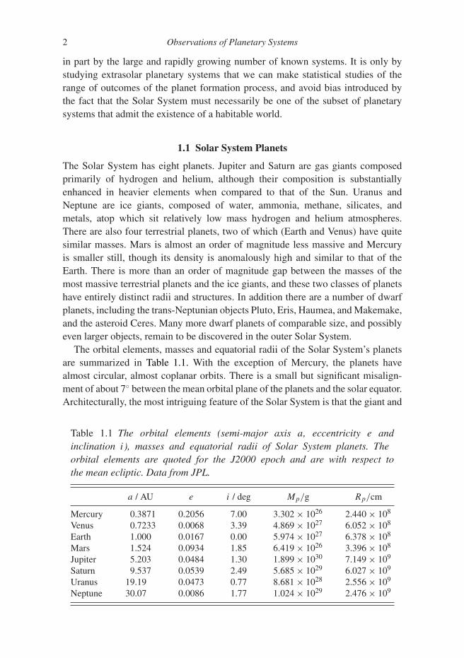
The Solar System has eight planets. Jupiter and Saturn are gas giants composedprimarily of hydrogen and helium, although their composition is substantiallyenhanced in heavier elements when compared to that of the Sun. Uranus andNeptune are ice giants, composed of water, ammonia, methane, silicates, andmetals, atop which sit relatively low mass hydrogen and helium atmospheres.There are also four terrestrial planets, two of which (Earth and Venus) have quitesimilar masses. Mars is almost an order of magnitude less massive and Mercuryis smaller still, though its density is anomalously high and similar to that of theEarth. There is more than an order of magnitude gap between the masses of themost massive terrestrial planets and the ice giants, and these two classes of planetshave entirely distinct radii and structures. In addition there are a number of dwarfplanets, including the trans-Neptunian objects Pluto, Eris, Haumea, and Makemake,and the asteroid Ceres. Many more dwarf planets of comparable size, and possiblyeven larger objects, remain to be discovered in the outer Solar System.
The orbital elements, masses and equatorial radii of the Solar System’s planetsare summarized in Table 1.1. With the exception of Mercury, the planets havealmost circular, almost coplanar orbits. There is a small but significant misalign-ment of about 7◦ between the mean orbital plane of the planets and the solar equator.Architecturally, the most intriguing feature of the Solar System is that the giant and
Table 1.1 The orbital elements (semi-major axis a, eccentricity e andinclination i), masses and equatorial radii of Solar System planets. Theorbital elements are quoted for the J2000 epoch and are with respect tothe mean ecliptic. Data from JPL.
a / AU e i / deg Mp/g Rp/cm
Mercury 0.3871 0.2056 7.00 3.302 × 1026 2.440 × 10⁸
Venus 0.7233 0.0068 3.39 4.869 × 1027 6.052 × 10⁸
Earth 1.000 0.0167 0.00 5.974 × 1027 6.378 × 10⁸
Mars 1.524 0.0934 1.85 6.419 × 1026 3.396 × 10⁸
Jupiter 5.203 0.0484 1.30 1.899 × 1030 7.149 × 10⁹
Saturn 9.537 0.0539 2.49 5.685 × 1029 6.027 × 10⁹
Uranus 19.19 0.0473 0.77 8.681 × 1028 2.556 × 10⁹
Neptune 30.07 0.0086 1.77 1.024 × 1029 2.476 × 10⁹

1.1 Solar System Planets 3
terrestrial planets are clearly segregated in orbital radius, with the giants only beingfound at large radii where the Solar Nebula (the disk of gas and dust from whichthe planets formed) would have been cool and icy.
The planets make a negligible contribution (� 0.13%) to the mass of the SolarSystem, which overwhelmingly resides in the Sun. The mass of the Sun, M� =1.989×1033 g, is made up of hydrogen (fraction by mass in the envelope X = 0.73),helium (Y = 0.25), and heavier elements (described in astronomical parlance as“metals,” with Z = 0.02). One notes that even most of the condensible elementsin the Solar System are in the Sun. This means that if a significant fraction ofthe current mass of the Sun passed through a disk during the formation epoch theprocess of planet formation need not be 100% efficient in converting solid materialin the disk into planets. In contrast to the mass, most of the angular momentumof the Solar System is locked up in the orbital angular momentum of the planets.Assuming rigid rotation at angular velocity �, the solar angular momentum can bewritten as
J� = k2M�R2��, (1.1)
where R� = 6.96 × 1010 cm is the solar radius. Taking � = 2.9 × 10⁻⁶ s−1 (thesolar rotation period is 25 dy), and adopting k2 ≈ 0.1 (roughly appropriate for astar with a radiative core), we obtain as an estimate for the solar angular momentumJ� ∼ 3×1048 g cm2 s−1. For comparison, the orbital angular momentum associatedwith Jupiter’s orbit at semi-major axis a is
JJ = MJ
√GM�a � 2 × 1050 g cm2 s−1. (1.2)
Even this value is small compared to the typical angular momentum contained inmolecular cloud cores that collapse to form low mass stars. We infer that substantialsegregation of angular momentum and mass must have occurred during the starformation process.
The orbital radii of the planets do not exhibit any relationships that yield imme-diate clues as to their formation or early evolution. (We briefly mention the Titius–Bode law in Section 7.4.3, but this empirical relation is not thought to have anyfundamental basis.) From a dynamical standpoint the most relevant fact is thatalthough the planets orbit close enough to perturb each other’s orbits, the perturba-tions are all nonresonant. Resonances occur when characteristic frequencies of twoor more bodies display a near-exact commensurability. They adopt disproportionateimportance in planetary dynamics because, in systems where the planets do notmake close encounters, gravitational forces between the planets are generally muchsmaller (typically by a factor of 103 or more) than the dominant force from thestar. These small perturbations are largely negligible unless special circumstances(i.e. a resonance) cause them to add up coherently over time. The simplest type of

4 Observations of Planetary Systems
resonance, known as a mean-motion resonance (MMR), occurs when the periodsP1 and P2 of two planets satisfy
P1
P2� i
j, (1.3)
where i and j are integers and use of the approximate equality sign denotes the factthat such resonances have a finite width. One can, of course, always find a pair ofintegers such that this equation is satisfied for arbitrary P1 and P2, so a more precisestatement is that there are no dynamically important resonances among the majorplanets.1 Nearest to resonance in the Solar System are Jupiter and Saturn, whosemotion is affected by their proximity to a 5:2 mean-motion resonance known as the“great inequality” (the existence of this near resonance, though not its dynamicalsignificance, was known even to Kepler). Among lower mass objects Pluto is oneof a large class of Kuiper Belt Objects (KBOs) in 3:2 resonance with Neptune,and there are many examples of important resonances among satellites and in theasteroid belt.
1.2 The Minimum Mass Solar Nebula
The mass of the disk of gas and dust that formed the Solar System is unknown.However, it is possible to use the observed masses, orbital radii and compositionsof the planets to derive a lower limit for the amount of material that must havebeen present, together with a crude idea as to how that material was distributedwith distance from the Sun. This is called the “minimum mass Solar Nebula”(Weidenschilling,1977a). The procedure is simple:
(1) Starting from the observed (or inferred) masses of heavy elements such as ironin the planets, augment the mass of each planet with enough hydrogen andhelium to bring the augmented mixture to solar composition.
(2) Divide the Solar System up into annuli, such that each annulus is centered onthe current semi-major axis of a planet and extends halfway to the orbit of theneighboring planets.
(3) Imagine spreading the augmented mass for each planet across the area of itsannulus. This yields a characteristic gas surface density � (units g cm−2) at thelocation of each planet.
Following this scheme, out to the orbital radius of Neptune the derived surfacedensity scales roughly as �(r) ∝ r−3/2. Since the procedure for constructing the
1 Roughly speaking, a resonance is typically dynamically important if the integers i and j (or their difference)are small. Care is needed, however, since although the 121:118 mean-motion resonance between Saturn’smoons Prometheus and Pandora formally satisfies this condition (since the difference is small) one would notimmediately suspect that such an obscure commensurability would be significant.
1.2 The Minimum Mass Solar Nebula 5
distribution is somewhat arbitrary it is possible to obtain a number of differentnormalizations, but the most common value used is that quoted by Hayashi (1981):
�(r) = 1.7 × 10³( r
1 AU
)−3/2g cm−2. (1.4)
Integrating this expression out to 30 AU the enclosed mass works out to be 0.01 M�,which is comparable to the estimated masses of protoplanetary disks around otherstars (though these have a wide spread). Hayashi (1981) also provided an estimatefor the surface density of solid material as a function of radius in the disk:
�s(rock) = 7.1( r
1 AU
)−3/2g cm−2 for r < 2.7 AU, (1.5)
�s(rock/ice) = 30( r
1 AU
)−3/2g cm−2 for r > 2.7 AU. (1.6)
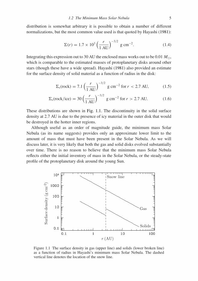
These distributions are shown in Fig. 1.1. The discontinuity in the solid surfacedensity at 2.7 AU is due to the presence of icy material in the outer disk that wouldbe destroyed in the hotter inner regions.
Although useful as an order of magnitude guide, the minimum mass SolarNebula (as its name suggests) provides only an approximate lower limit to theamount of mass that must have been present in the Solar Nebula. As we willdiscuss later, it is very likely that both the gas and solid disks evolved substantiallyover time. There is no reason to believe that the minimum mass Solar Nebulareflects either the initial inventory of mass in the Solar Nebula, or the steady-stateprofile of the protoplanetary disk around the young Sun.
Solids
Gas
Snow line
r (AU)
Surf
ace
dens
ity
(g c
m-2)
Figure 1.1 The surface density in gas (upper line) and solids (lower broken line)as a function of radius in Hayashi’s minimum mass Solar Nebula. The dashedvertical line denotes the location of the snow line.
6 Observations of Planetary Systems
1.3 Minor Bodies in the Solar System
In addition to the planets, the Solar System contains a wealth of minor bodies:asteroids, Trans-Neptunian Objects (TNOs, including those in the Kuiper Belt),comets, and planetary satellites. The total mass in these reservoirs is now small.2
The main asteroid belt has a mass of about 5 × 10⁻⁴ M⊕ (Petit et al., 2001), whilethe more uncertain estimates for the Kuiper Belt are of the order of 0.1 M⊕ (Chianget al., 2007). Although dynamically unimportant, the distribution of minor bodiesis extremely important for the clues it provides to the early history of the SolarSystem. As a very rough generalization the Solar System is dynamically full, in thesense that most locations where small bodies could stably orbit for billions of yearsare, in fact, populated. In the inner Solar System, the main reservoir is the mainasteroid belt between Mars and Jupiter, while in the outer Solar System the KuiperBelt is found beyond the orbit of Neptune.
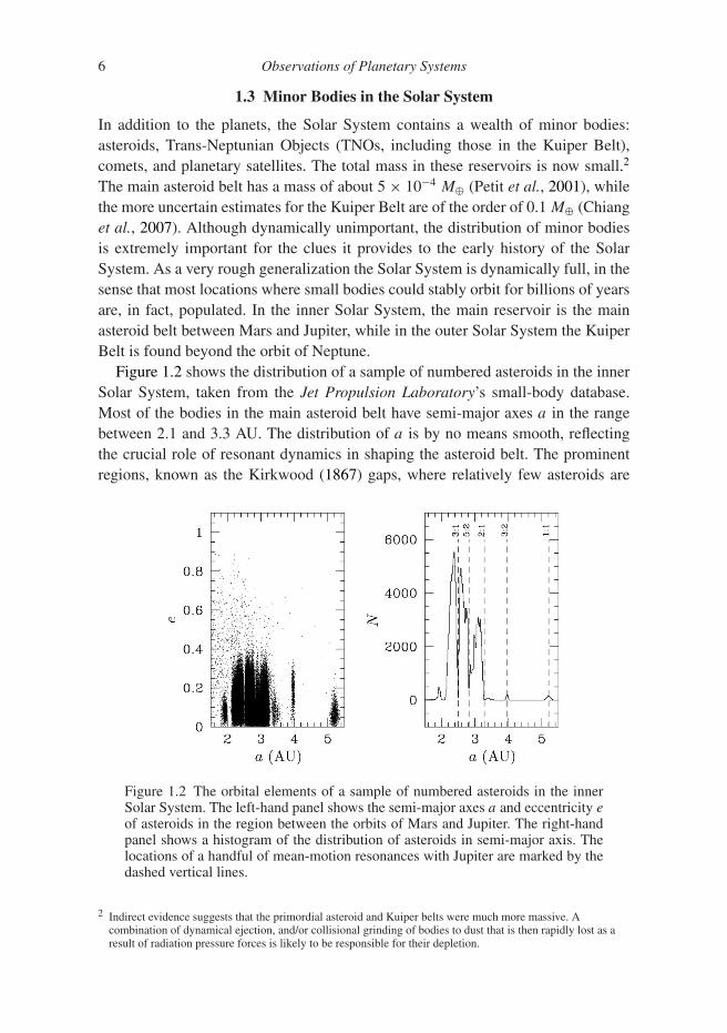
Figure 1.2 shows the distribution of a sample of numbered asteroids in the innerSolar System, taken from the Jet Propulsion Laboratory’s small-body database.Most of the bodies in the main asteroid belt have semi-major axes a in the rangebetween 2.1 and 3.3 AU. The distribution of a is by no means smooth, reflectingthe crucial role of resonant dynamics in shaping the asteroid belt. The prominentregions, known as the Kirkwood (1867) gaps, where relatively few asteroids are
Figure 1.2 The orbital elements of a sample of numbered asteroids in the innerSolar System. The left-hand panel shows the semi-major axes a and eccentricity eof asteroids in the region between the orbits of Mars and Jupiter. The right-handpanel shows a histogram of the distribution of asteroids in semi-major axis. Thelocations of a handful of mean-motion resonances with Jupiter are marked by thedashed vertical lines.
2 Indirect evidence suggests that the primordial asteroid and Kuiper belts were much more massive. Acombination of dynamical ejection, and/or collisional grinding of bodies to dust that is then rapidly lost as aresult of radiation pressure forces is likely to be responsible for their depletion.

1.3 Minor Bodies in the Solar System 7
found coincide with the locations of mean-motion resonances with Jupiter, mostnotably the 3:1 and 5:2 resonances. In addition to these locations – at whichresonances with Jupiter are evidently depleting the population of minor bod-ies – there are concentrations of asteroids at both the co-orbital 1:1 resonance(the Trojan asteroids), and at the interior 3:2 resonance (the Hilda asteroids).This is a graphic demonstration of the fact that different resonances can eitherdestabilize or protect asteroid orbits (for a thorough analysis of the dynamicsinvolved the reader should consult Murray & Dermott, 1999). Also notable isthat the asteroids, unlike the major planets, have a distribution of eccentricitye that extends to moderately large values. Between 2.1 and 3.3 AU the meaneccentricity of the numbered asteroids is 〈e〉 � 0.14. As a result, collisions inthe asteroid belt today typically involve relative velocities that are large enoughto be disruptive. Indeed, a number of asteroid families (Hirayama, 1918) areknown, whose members share similar orbital elements (a,e,i). These asteroids areinterpreted as debris from disruptive collisions taking place within the asteroidbelt, in some cases relatively recently (within the last few Myr, e.g. Nesvornyet al., 2002).
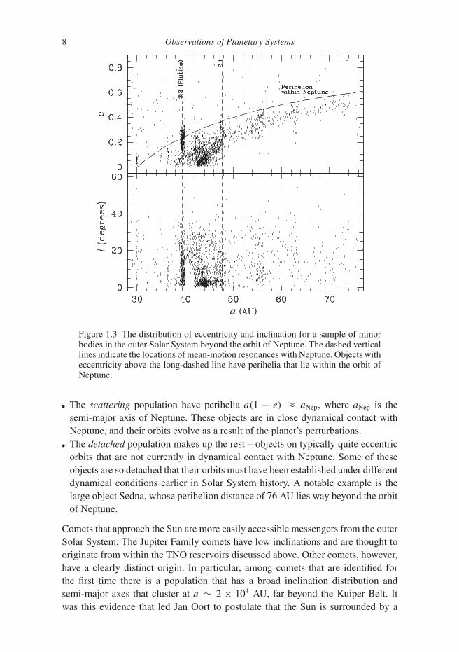
Figure 1.3 shows the distribution of a sample of outer Solar System bodies,maintained by the IAU’s Minor Planet Center. Among the known planets outerSolar System bodies interact most strongly with Neptune, and to leading order theyare classified based upon the nature of that interaction.
• Resonant Kuiper Belt Objects (KBOs) currently occupy mean-motion resonanceswith Neptune. The most common resonance is the 3:2 that is occupied by Pluto,and such objects are also called Plutinos. The eccentricity of some Plutinos –including Pluto itself – is large enough that their perihelion lies within the orbitof Neptune, and these objects depend upon their resonant configuration to avoidclose encounters. The existence of this large population of moderately eccentricresonant bodies provided the original evidence for models in which Neptunemigrated outward early in Solar System history.
• Classical KBOs orbit in a relatively narrow belt between Neptune’s 3:2 and 2:1MMRs (39.5AU < a < 47.8 AU), and their number drops sharply toward theupper end of this range of semi-major axes (Trujillo & Brown, 2001). Theseobjects are nonresonant and they have low enough eccentricity to avoid scat-tering encounters with Neptune. They can be divided into two sub-populations.The cold classical belt objects have lower inclinations i < 2◦ (and generallyalso lower eccentricities) than the hot objects, which have i > 6◦ (Dawson &Murray-Clay, 2012). (Objects with intermediate inclinations cannot be classifiedreliably using only orbital information.) The dynamical classification matches upto apparent physical differences that are inferred from measurements of the colorand size distribution, which suggests that the cold and hot populations derive fromdistinct source populations.
8 Observations of Planetary Systems
)
)
i
a ( )
Figure 1.3 The distribution of eccentricity and inclination for a sample of minorbodies in the outer Solar System beyond the orbit of Neptune. The dashed verticallines indicate the locations of mean-motion resonances with Neptune. Objects witheccentricity above the long-dashed line have perihelia that lie within the orbit ofNeptune.
• The scattering population have perihelia a(1 − e) ≈ aNep, where aNep is thesemi-major axis of Neptune. These objects are in close dynamical contact withNeptune, and their orbits evolve as a result of the planet’s perturbations.
• The detached population makes up the rest – objects on typically quite eccentricorbits that are not currently in dynamical contact with Neptune. Some of theseobjects are so detached that their orbits must have been established under differentdynamical conditions earlier in Solar System history. A notable example is thelarge object Sedna, whose perihelion distance of 76 AU lies way beyond the orbitof Neptune.
Comets that approach the Sun are more easily accessible messengers from the outerSolar System. The Jupiter Family comets have low inclinations and are thought tooriginate from within the TNO reservoirs discussed above. Other comets, however,have a clearly distinct origin. In particular, among comets that are identified forthe first time there is a population that has a broad inclination distribution andsemi-major axes that cluster at a ∼ 2 × 10⁴ AU, far beyond the Kuiper Belt. Itwas this evidence that led Jan Oort to postulate that the Sun is surrounded by a
1.4 Radioactive Dating of the Solar System 9
quasi-spherical reservoir of comets, now called the Oort cloud (Oort, 1950). TheOort cloud was established at an early epoch and delivers comets toward the innerSolar System over time as a consequence of Galactic tidal forces and perturbationsfrom passing stars.
Planetary satellites in the Solar System also fall into several classes. The regularsatellites of Jupiter, Saturn, Uranus, and Neptune have relatively tight progradeorbits that lie close to the equatorial plane of their respective planets. This suggeststhat these satellites formed from disks, analogous to the Solar Nebula itself, thatsurrounded the planets shortly after their formation. The total masses of the regularsatellite systems are a relatively constant fraction (about 10−4) of the mass of thehost planet, with the largest satellite, Jupiter’s moon Ganymede, having a mass of0.025 M⊕. The presence of resonances between different satellite orbits – mostnotably the Laplace resonance that involves Io, Europa, and Ganymede (Io lies in2:1 resonance with Europa, which in turn is in 2:1 resonance with Ganymede) – isstriking. As in the case of Pluto’s resonance with Neptune, the existence of thesenontrivial configurations among the satellites provides evidence for past orbitalevolution that was followed by resonant capture. Orbital migration within a pri-mordial disk, or tidal interaction with the planet, are candidates for explaining theseresonances.
The giant planets also possess extensive systems of irregular satellites, whichare typically more distant and which do not share the common disk plane of theregular satellites. These satellites were probably captured by the giant planets fromheliocentric orbits.
The sole example of a natural satellite of a terrestrial planet – the Earth’s Moon –is distinctly different from any giant planet satellite. Relative to its planet it is muchmore massive (the Moon is more than 1% of the mass of the Earth), and its orbitalangular momentum makes up most of the angular momentum of the Earth–Moonsystem. The Moon’s composition is not the same as that of the Earth; there is lessiron (resulting in a lower density than the uncompressed density of the Earth) andevidence for depletion of some volatile elements. Some aspects of the composition,in particular the ratios of stable isotopes of oxygen, are however essentially indis-tinguishable from those measured from terrestrial mantle samples. Qualitativelythese properties are interpreted within models in which the Moon formed from thecooling of a heavy-element rich disk generated following a giant impact early in theEarth’s history (Hartmann & Davis, 1975; Cameron & Ward, 1976), though someof the quantitative constraints remain challenging to reproduce. Pluto’s large moonCharon may have formed in the aftermath of a similar impact.
1.4 Radioactive Dating of the Solar System
Determining the ages of individual stars from astronomical observations is a dif-ficult exercise, and good constraints are normally only possible if the frequen-cies of stellar oscillations can be identified via photometric or spectroscopic data.

10 Observations of Planetary Systems
Much more accurate age determinations are possible for the Solar System, viaradioactive dating of apparently pristine samples from meteorites.
It is worth clarifying at the outset how radioactive dating works, because it isnot as simple as one might initially think. Consider a notional radioactive decayA → B that occurs with mean lifetime τ . After time t the abundance nA of “A” isreduced from its initial value nA0 according to
nA = nA0e−t/τ, (1.7)
while that of “B” increases,
nB = nB0 + nA0(1 − e−t/τ ). (1.8)
We can assume that τ is known precisely from laboratory measurements. However,it is clear that we cannot in general determine the age because we have threeunknowns (t and the initial abundances of the two species) but only two observables(the current abundances of each species). Getting around this roadblock requiresconsidering more complex decays and imposing assumptions about how the sam-ples under consideration formed in the first place.
For a simple example that works we can look at a rock containing radioactivepotassium (40K) that solidifies from the vapor or liquid phases during the epoch ofplanet formation. One of the decay channels of 40K is
40K → 40Ar. (1.9)
This decay has a half-life of 1.25 Gyr and a branching ratio ξ ≈ 0.1. (The branchingratio describes the probability that the radioactive isotope decays via a specificchannel. In this case ξ is small because 40K decays more often into 40Ca.) If weassume that the rock, once it has solidified, traps the argon and that there wasno argon in the rock to start with, then we have eliminated one of the generallyunknown quantities and measuring the relative abundance of 40Ar and 40K suf-fices to determine the age. Quantitatively, if the parent isotope 40K has an initialabundance np(0) when the rock solidifies at time t = 0, then at later times theabundances of the parent isotope np and daughter isotope nd are given by the usualexponential formulae that characterize radioactive decay:
np = np(0)e−t/τ,
nd = ξnp(0)[1 − e−t/τ
],
(1.10)
where τ , the mean lifetime, is related to the half-life via τ = t1/2/ln 2. The ratio ofthe daughter to parent abundance is
nd
np= ξ
(et/τ − 1
). (1.11)
A laboratory measurement of the left-hand-side then fixes the age provided thatthe nuclear physics of the decay (the mean lifetime and the branching ratio) is

1.4 Radioactive Dating of the Solar System 11
accurately known. Notice that this method works to date the age of the rock (ratherthan the epoch when the radioactive potassium was formed) because mineralshave distinct chemical compositions that differ – often dramatically so – fromthe average composition of the protoplanetary disk. In the example above, it isreasonable to assume that any 40Ar atoms formed prior to the rock solidifying willnot be incorporated into the rock, first because the argon will be diluted throughoutthe disk and second because it is an unreactive element that will not be part of thesame minerals as potassium.
Radioactive dating is also possible in systems where we cannot safely assumethat the initial abundance of the daughter isotope is negligible. The decay of rubid-ium 87 into strontium 87,
87Rb →87 Sr, (1.12)
occurs with a half-life of 48.8 Gyr. Unlike argon, strontium is not a noble gas, andwe cannot assume that the rock is initially devoid of strontium. If we denote theinitial abundance of the daughter isotope as nd(0), then measurement of the ratio(nd/np) yields a single constraint on two unknowns (the initial daughter abundanceand the age) and dating appears impossible. Again, the varied chemical propertiesof rocks allow progress. Suppose we measure samples from two different mineralswithin the same rock, and compare the abundances of 87Rb and 87Sr not to eachother, but to the abundance of a separate stable isotope of strontium 86Sr. Since 86Sris chemically identical to the daughter isotope 87Sr that we are interested in, it isreasonable to assume that the ratio 87Sr/86Sr was initially constant across samples.The ratio 87Rb/86Sr, on the other hand, can differ between samples. As the rockages, the abundance of the parent isotope drops and that of the daughter increases.Quantitatively,
np = np(0)e−t/τ,
nd = nd(0) + ξnp(0)[1 − e−t/τ
].
(1.13)
Eliminating np(0) between these equations and dividing by the abundance nds ofthe second stable isotope of the daughter species (86Sr in our example) we obtain(
nd
nds
)=
(nd(0)
nds
)+ ξ
(np
nds
) [et/τ − 1
]. (1.14)
The first term on the right-hand-side is a constant. We can then plot the rela-tive abundances of the parent isotope (np/nds) and the daughter isotope (nd/nds)
from different samples on a ratio–ratio plot called an isochron diagram, such asthe one shown schematically in Fig. 1.4. Inspection of Eq. (1.14) shows that weshould expect the points from different samples to lie on a straight line whose slope(together with independent knowledge of the mean lifetime) fixes the age. Twosamples are in principle sufficient to yield an age determination, but additional data

12 Observations of Planetary Systems
87Rb / 86Sr
87S
r / 86
Sr
t = 0
t = t1
t = t2
Sample #1 Sample #2
Figure 1.4 Ratio–ratio plot for dating rocks using the radioactive decay87Rb →87Sr. The abundance of these isotopes is plotted relative to the abundanceof a separate stable isotope of strontium 86Sr. When the rock solidifies, differentsamples contain identical ratios of 87Sr/86Sr, but different ratios of 87Rb/86Sr.The ratios of different samples track a steepening straight line as the rock ages.
provide a check against possible systematic errors. If the points fail to lie on astraight line something is wrong.
1.4.1 Lead–Lead Dating
The most important system for absolute determination of the age of Solar Systemsamples, lead–lead dating, is based upon the measurement of lead and uraniumisotopes. Lead has four stable and naturally occurring isotopes with mass num-bers 204, 206, 207, and 208. Of these, 204Pb preserves its primordial abundance,while the abundance of the heavier isotopes increases over time because theseare daughter isotopes from the decay of uranium and thorium.The parent/daughterrelationships are
238U → 206Pb (t1/2 = 4.47 × 10⁹ yr),235U → 207Pb (t1/2 = 7.04 × 10⁸ yr), (1.15)
232Th → 208Pb (t1/2 = 1.40 × 10¹⁰ yr).
The relatively high abundance of the parent isotopes, coupled with the favorablehalf-lives, mean that this system is well suited to deliver ages of high accuracy andprecision.
There are several ways to derive dates using the above system. Limiting attentionto the two uranium decays gives a pair of equations analogous to Eq. (1.14):( 206Pb
204Pb
)=
( 206Pb204Pb
)0
+( 238U
204Pb
) [et/τ1 − 1
], (1.16)( 207Pb
204Pb
)=
( 207Pb204Pb
)0
+( 235U
204Pb
) [et/τ2 − 1
]. (1.17)

1.4 Radioactive Dating of the Solar System 13
Here the ratios presented without subscripts are the present-day (measurable) val-ues, while those with the subscript “0” refer to the initial values at the time whenthe system became closed. The mean lifetimes τ1 and τ2 refer to the decay of 238Uand 235U. At this point we could, following the logic above, make two ratio–ratioplots (e.g. from the first equation 206Pb/204Pb against 238U/204Pb) and derive twoindependent ages from a single sample of primitive material. It turns out, how-ever, that we can do a better job at reducing practical sources of error (associated,for example, with terrestrial contamination) by considering the two uranium/leadsystems jointly. By taking the ratio of Eq. (1.17) to Eq. (1.16) we obtain a form inwhich the left-hand-side depends only on initial or current lead isotope ratios, whilethe right-hand-side depends only on the current uranium isotope ratio:
(207Pb/204Pb) − (207Pb/204Pb)0
(206Pb/204Pb) − (206Pb/204Pb)0=
( 235U238U
)(et/τ1 − 1
et/τ2 − 1
). (1.18)
Multiplying first by the denominator and then by (204Pb/206Pb) shows that a ratio–ratio plot of (204Pb/206Pb) versus (207Pb/206Pb) ought to give a straight line:( 207Pb
206Pb
)=
( 235U238U
)(et/τ1 − 1
et/τ2 − 1
)︸ ︷︷ ︸
intercept
+ b(t)
( 204Pb206Pb
). (1.19)
(Here b(t) is an age-dependent constant whose exact form is not important for ourpurposes.) Measuring the intercept from a ratio–ratio plot involving the three leadisotopes, along with a current determination of the uranium isotope ratio, yields ameasure of the sample age.
Connelly et al. (2017) review both the theory and the practical difficultiesencountered in lead–lead dating of Solar System samples. Astonishingly, agedeterminations using this method are able to resolve events at the dawn of the SolarSystem, 4.57 Gyr ago, with a precision that is of the order of 0.2 Myr.
1.4.2 Dating with Short-Lived Radionuclides
Absolute chronometry provides an estimated age for the earliest Solar Systemsolids of 4.5673 ± 0.0002 Gyr (Connelly et al., 2017). This is the measurablequantity that, by convention, is described as the “age of the Solar System.”Knowing the age of the Sun is useful for calibrating solar evolution models,but the exact absolute age is otherwise superfluous for studies of planet formation.More valuable are constraints on the time scale of critical phases of the planetformation process. For example, it is of interest to know whether the formationof the km-sized bodies called planetesimals was sudden or spread out over manyMyr. Questions of this kind, which involve only relative ages, can of course beaddressed given sufficiently accurate absolute chronometry. A complementaryapproach determines only relative ages from the decay products of short-livedisotopes. It is well established that the Solar Nebula initially contained radioactive

14 Observations of Planetary Systems
species with very short half-lives, including 26Al which has a half-life of only0.72 Myr. The likely origin of these isotopes is nucleosynthesis within the coresof massive stars followed by ejection into the surrounding medium via either asupernova explosion or Wolf–Rayet stellar winds. In either case the implication isthat the Sun formed in proximity to a rich star forming region (or within a cluster,now dissolved) that also contained massive stars.
Heating due to the radioactive decay of 26Al is important for the thermal evo-lution of small bodies forming within protoplanetary disks, and the ionization pro-duced from these decays may also be physically significant. For dating, the keypoint is that we can learn something about the relative ages of samples by measuringthe abundance of daughter isotopes even when all of the parent species has longsince decayed. For example, we could imagine measuring the abundance of 129Xe,formed via the decay,
129I → 129Xe, (1.20)
and comparing it to the abundance of a stable isotope of iodine 127I. The 129I decayhas a a half-life of only 17 Myr. Accordingly, we would expect that samples thatform early would incorporate a higher (129I/127I) ratio, and this would lead to ahigher (129Xe/127I) ratio that is preserved at late times after all of the radioactiveiodine is gone.
The main caveat to be borne in mind with radioactive dating (both absolute andrelative) is that it depends upon there being no other processes besides radioac-tive decay that alter the abundance of either the parent or daughter isotopes. Theradioactive age of a rock measures the moment it solidified only if there has been nodiffusion, or other alteration of the rock, during the intervening period. Even if therock itself is pristine, high energy particles (cosmic rays) can induce nuclear reac-tions that may change the abundances of some critical isotopes. Relative chronom-etry additionally relies on the assumed spatial homogeneity of the parent specieswithin the disk. Because the half-lives of the species used for relative dating areshort, there may not have been enough time for the short-lived parents to have beenmixed throughout the gas that forms the disk, and the assumption of homogeneitycan reasonably be questioned.
1.5 Ice Lines
Liquid water is not stable under the low pressure conditions of the gaseous proto-planetary disk. Water ice, which is abundant at low temperature, sublimates directlyto vapor in regions of the disk where the temperature exceeds about 150–170 K.The radial location in the disk beyond which the temperature falls below this valueis called the snow line. Analogous “ice lines” exist for other common chemicalspecies. The carbon monoxide (CO) ice line corresponds to a temperature of23–28 K, while the carbon dioxide (CO2) ice line is predicted to be at 60–72 K.

1.5 Ice Lines 15
Theoretically, the location of the snow line is expected to change over time,due to variations in the stellar luminosity and in the rate at which gas is beingaccreted through the disk (as we will discuss in Chapter 3, accretion can be animportant source of heat). For a solar mass, solar luminosity star, accreting at anobservationally typical rate, the snow line is predicted to lie between 1 and 2 AU.Reasonable variations of these parameters lead to snow lines between about 0.5and 5 AU (Garaud & Lin, 2007). Observationally, the location of the snow line isdifficult to pin down from astronomical data on protoplanetary disks, and hence themain constraints come from laboratory measurement of meteoritic samples. Mete-orites of the class known as carbonaceous chondrites, which are water-rich, haveproperties (such as their reflectance spectra) that match those of asteroids foundonly in the outer asteroid belt beyond about 2.5 AU. Conversely, the ordinary andenstatite chondrites, which contain negligible amounts of water, appear to originatefrom the inner asteroid belt at a distance from the Sun of around 2 AU. Consistentwith this, the dwarf planet Ceres in the outer asteroid belt is known to have bothsurface and sub-surface water, and may contain a substantial interior water reser-voir. The empirical conclusion is that compositional variations in the asteroid beltpreserve evidence for a snow line in the early Solar Nebula at about a � 2.7 AU.
The location of the snow line has important consequences for the compositionand habitability of terrestrial planets. The standard definition of the “habitablezone” for terrestrial planets is based on requiring that liquid water is stable onthe surface. Under Earth’s atmospheric pressure, that translates into a surfacetemperature between 273 K < T < 373 K. As noted above, however, the lowerpressure in the disk gas means that prior to planet formation water would haveexisted only in the vapor phase at temperatures above T � 150–170 K. This leadsto a somewhat surprising prediction; planets that formed in situ within the habitablezone are typically assembled from planetesimals that formed interior to the snowline in a region of the disk that would have been too hot for water-rich minerals tocondense. Solar System evidence for a snow line at 2.7 AU supports this scenariofor the Earth.
The idea that habitable planets form inside the snow line is consistent not justwith Solar System meteoritic evidence, but with the first-order composition of theEarth. Surface appearances to the contrary, the Earth is not a water world. The massof water in the ocean, atmosphere, and crust of the Earth is just 2.8 × 10⁻⁴ M⊕(where the Earth mass, M⊕ = 5.974 × 1027 g). The amount of extra water lockedin the mantle is uncertain (especially early in the Earth’s history) and could besubstantial, but it is clear that the total water fraction is orders of magnitude belowthat found in ice-rich bodies beyond the snow line.
Several models have been proposed to explain where the Earth’s water camefrom. The leading hypothesis is that water was delivered to the Earth from areservoir of small bodies (asteroids, comets, or a now vanished class of objects)beyond the snow line. Alternatively, Solar System material at 1 AU may have

16 Observations of Planetary Systems
contained a small admixture of water (in the form of water molecules that can bindto some grain surfaces at relatively high temperature), and not have been as dry as isassumed in the standard model. The isotopic makeup of the Earth’s water providesa constraint. The reference value for the deuterium to hydrogen (D/H) ratio of waterin the Earth’s ocean is 156 parts per million (ppm), in broad agreement with themean 159±10 ppm measured in carbonaceous chondrites (Morbidelli et al., 2000).Data on comets are more limited, but values measured for Oort cloud comets aresubstantially higher (around 300 ppm). Hartogh et al. (2011) reported an Earth-likevalue of ≈160 ppm for the Jupiter family comet 103P/Hartley 2, but a much higherratio of ≈530 pm was measured for 67P/Churyumov–Gerasimenko (the comet,also from the Jupiter family, which was the target of the Rosetta mission; Altwegget al., 2015).
Given the admittedly inconclusive evidence, the most likely source for the bulkof the Earth’s water is asteroids from the outer part of the main belt. The mass ofasteroids required is substantial. If our water arrived via asteroids with compositionssimilar to the carbonaceous chondrites, which have mass fractions of water of≈10%, the total mass required would have been a few 10−3 M⊕. Although thismass is negligible on the scale of the impacts that assembled the Earth and formedthe Moon, it still exceeds the total mass in the present-day asteroid belt by an orderof magnitude.
1.6 Meteoritic and Solar System Samples
Unique but sometimes hard to interpret information about conditions in the SolarNebula comes from the study of Solar System samples, recovered from meteoritesand from a handful of sample return missions. Meteorites originate from the aster-oid belt, the Moon, and Mars, and have a composition that reflects the structureof their parent bodies. Undifferentiated bodies, which are generally smaller, neverbecame hot enough to form a distinct core/mantle/crust structure. They give rise tochondritic meteorites, which once the most volatile elements are excluded have abulk chemical composition that is similar to that of the Sun. Differentiated bodies,by contrast, are the progenitors of iron meteorites (made up of iron–nickel alloys)and achondrites, stony meteorites that are mostly made up of igneous rocks.
The chondritic meteorites are divided into numerous classes and are not, for themost part, entirely pristine. Their minerals often show evidence for changes thatoccurred on the parent body due to the action of heat and/or water. The carbona-ceous chondrites are among the least altered (or most “primitive”), and togetherwith samples returned directly from comets and asteroids represent the closestapproximation to early Solar System material that can be studied in the laboratory.
The rock of chondritic meteorites is a mixture of three quite distinct components:refractory inclusions, chondrules, and matrix. The refractory inclusions – calcium,aluminium-rich inclusions (CAIs), and amoeboid olivine aggregates – have a

1.6 Meteoritic and Solar System Samples 17
chemical composition and structure that suggest that they formed at temperaturesin excess of 1350 K. Both absolute and relative dating support the idea thatCAIs are the oldest known Solar System materials, with an age estimated at4.5673 ± 0.0002 Gyr (Connelly et al., 2017). The dispersion in the inferred ages ofCAIs is small, suggesting that they may have formed under high temperature diskconditions, presumably close to the Sun, during the earliest stage of disk evolution.
Chondrules are a second high temperature component of chondrites. Chon-drules are typically 0.1–1 mm spheres of igneous rock that make up a vari-able but often large fraction of chondritic meteorites (as much as 80% of thevolume of ordinary and enstatite chondrites, and 0 to 70% of carbonaceouschondrites; Nittler & Ciesla, 2016). The most basic fact about chondrules,indicated by their spherical shape and mineral texture, is that they formed dueto cooling of initially molten precursors. A great deal is known experimentallyabout what happens as igneous rocks cool and crystallize, and as a consequencethere are surprisingly informative constraints on the conditions under whichchondrules formed (Desch et al., 2012; Nittler & Ciesla, 2016). It is gener-ally accepted that chondrule precursors – the solid particles or material thatwere melted to become chondrules – formed under relatively low temperatureconditions, because chondrules contain FeS, which would not be present atT >∼ 650 K. The precursor material was then heated rapidly, on a time scaleof at most minutes, to a temperature of about 2000 K. Volatile elements, suchas Na and K, may have been lost while the chondrule was molten, but did notexperience the mass-dependent isotope fractionation that would be expectedif they were surrounded by a low–pressure gas. This implies formation in arelatively large high density environment where evaporation and fractionationare suppressed by the development of a volatile-rich vapor. After melting, thevarious mineral textures observed in chondrules suggest cooling at rates betweenabout 10 K per hour and 104 K per hour. Even the top end of this range is orders ofmagnitude below the cooling rate expected for a single small sphere radiatingfreely to space, implying again that the formation regions were large enough sothat radiative transfer effects slowed the cooling rate. Both absolute and relativechronometry show that chondrules did not form before CAIs. Some chondrulesmay have formed at roughly the same time as refractory inclusions, but othersformed several Myr later.
The third component of chondritic meteorites is matrix, small micrometer-sized particles of minerals such as crystalline magnesian olivine, pyroxene, andamorphous ferromagnesian silicates. Matrix materials contain a larger fraction ofvolatile elements, consistent with formation under lower temperature conditionsthan those needed for either CAI or chondrule formation. The average compositionof chondrules and matrix is, in a colloquial sense, “complementary,” in that theformer is depleted and the latter enriched in volatiles. The hypothesis of chemicalcomplementarity holds that this relationship also holds for individual chondrites.
18 Observations of Planetary Systems
Complementarity in this stricter sense would provide evidence that chondrules andmatrix formed from a common reservoir of disk gas.
Both CAIs and chondrules are found within meteorites whose parent bodiesorbited within the asteroid belt at orbital radii not far from the inferred locationof the snow line. At this radii there is almost an order of magnitude gulf betweenthe expected disk temperatures and those implicated in the formation of thesehigh temperature materials. For chondrules two main classes of models have beenproposed to explain how the required high temperature can be realized at 3 AUfrom the Sun. One holds that chondrules formed as pre-existing solid particlespassed through shock waves in the gas disk. The shock waves could have beeneither large-scale spiral shocks in the disk (although it is hard to see how thesewould form), or more localized bow shocks around orbiting planetary embryos.Alternatively, chondrules may have formed out of the cooling debris of planetesimalimpacts. For CAIs the standard scenario is that these materials formed withinthe disk, probably closer to the Sun, and were transported radially before beingincorporated into larger solid bodies.
The mystery of how CAIs and (especially) chondrules formed is one of the mostimportant open problems in meteoritics and cosmochemistry. The wider relevancefor planet formation cannot be determined without first knowing the answer. Allthat we know for sure is that the small mass currently in undifferentiated asteroidsis made up of a high fraction by mass of chondrules. If the formation mechanism forchondrules involved long-lived disk processes then it is reasonable to assume that alarge fraction of the solid material that forms terrestrial planets was once processedthrough a chondrule-like phase. Chondrules would then be generic precursors ofplanets. If, on the other hand, chondrules form from a process such as late planetes-imal collisions, they are bystanders of only peripheral interest for understanding themain phases of planet formation.
Results from the Stardust sample return mission from the Jupiter family cometWild 2 raise district but thematically related questions. Analysis of 1–10 μmparticles collected from the comet showed that many of them are made up ofolivine or pyroxene. These are crystalline silicates that can be produced fromamorphous precursors via annealing at temperatures of 800 K and above (Brownleeet al., 2006). This result implies that even the very cold regions of the disk wherecomets formed were somehow polluted with a fraction of material processedthrough high temperatures.
1.7 Exoplanet Detection Methods
The first extrasolar planetary system to be discovered was identified by Alex Wol-szczan and Dale Frail via precision timing of pulses from the millisecond pulsarPSR1257+12 (Wolszczan & Frail, 1992). The system contains at least three planets

1.7 Exoplanet Detection Methods 19
on nearly circular orbits within 0.5 AU of the neutron star, with the outer two planetshaving masses close to 4 M⊕ and the inner planet having a mass 0.02 M⊕ whichis comparable to the mass of the Moon. Millisecond pulsars are a type of rapidlyrotating neutron star that form in supernova explosions, and the mass loss during theexplosion would unbind any pre-existing planets. The planets in the PSR1257+12system must therefore have originated within a disk formed subsequent to theexplosion. The observation that pulsar planets are not common (Kerr et al., 2015)implies that the conditions leading to their formation could involve moderately rareevents.
The precision required to find Jupiter mass planets in relatively short-periodorbits via monitoring of the radial velocity of their host stars first became availablein the 1980s (Campbell et al., 1988). The first accepted detection, of 51 Peg b,a Jupiter mass body orbiting a solar-type star, was made using this technique byMichel Mayor and Didier Queloz in 1995 (Mayor & Queloz, 1995). The first twodecades of exoplanet discovery were dominated by detections made via the radialvelocity and transit methods, with smaller numbers of planets being found usingmicrolensing and direct imaging techniques. An additional technique, astrometry,is expected to play a growing role in future planet discovery. Based on existing datait is known that planets have a broad range of masses, from sub-Earth mass up to thedeuterium burning limit, and orbit all the way from 0.01 AU to 100 AU from theirhost star. No single planet discovery method is sensitive across this entire parameterspace, large fractions of which remain unexplored by any method. A synthesis ofmultiple surveys, each with its own selection function in planetary mass, radius, andorbital period, is needed to build up an understanding of the population of extrasolarplanetary systems.
1.7.1 Direct Imaging
The most straightforward way to detect extrasolar planets is to image the planetas a source of light that is spatially separated from the stellar emission. The maindifficulty is the extreme contrast between a planet and its host star. A planet ofradius Rp, orbital radius a, and albedo A intercepts and reflects a fraction f of theincident starlight given by
f =(
πR2p
4πa2
)A = 1.4 × 10⁻¹⁰
(A
0.3
)(Rp
R⊕
)2 ( a
1 AU
)−2. (1.21)
Recalling that magnitudes are defined in terms of the flux F via m = −2.5 log10 F+const, one finds that Earth-like planets are expected to be 24–25 magnitudes fainterthan their host stars. This faintness means that, quite apart from the very unfavorablecontrast ratio between planet and star, moderately deep exposures are needed tohave even a chance of directly imaging planets in reflected light. Alternatively, onemay contemplate imaging extrasolar planets in their thermal emission. If we crudely

20 Observations of Planetary Systems
approximate the emission at frequency ν from a planet with surface temperature T
as a blackbody, then the spectrum is described by the Planck function:
Bν(T ) = 2hν3
c2
1
exp(hν/kBT ) − 1, (1.22)
where h is Planck’s constant, c the speed of light, and kB the Boltzmann constant.The peak of the spectrum falls at hνmax = 2.8kBT , which lies in the mid-IR fortypical terrestrial planets (the wavelength corresponding to νmax is λ ≈ 20 μm forthe Earth with T = 290 K). If the star, with radius R∗, also radiates as a blackbodyat temperature T∗, the flux ratio at frequency ν is
f =(
Rp
R∗
)2 exp(hν/kBT∗) − 1
exp(hν/kBT ) − 1. (1.23)
For an Earth-analog around a solar-type star the contrast ratio for observations at awavelength of 20 μm is f ∼ 10−6, which is some four orders of magnitude morefavorable than the corresponding ratio in reflected light. This advantage of workingin the infrared is, however, offset by the need for a larger telescope in order tospatially resolve the planet. The spatial resolution of a telescope of diameter D
working at a wavelength λ is
θ ∼ 1.22λ
D. (1.24)
A spatial resolution of 0.5 AU at a distance of 5 pc corresponds to an angular reso-lution of 0.1 arcsec, which is theoretically achievable in the visible (λ = 550 nm)with a telescope of diameter D ≈ 1.5 m. At 20 μm, on the other hand, the requireddiameter balloons to D ≈ 50 m, which is unfeasibly large to contemplate construct-ing as a monolithic structure in space.
These elementary considerations show that the difficulty of directly imagingplanets depends strongly on their orbital radii. Giant planets orbiting at large orvery large radii (tens of AU) are relatively easy to image, with known examplesincluding the multiple planets of the HR 8799 system (Marois et al., 2008). State-of-the-art direct imaging surveys employ a combination of telescope hardware andnovel modes of observation to overcome the unfavorable contrast ratio between starand planet. Adaptive optics can recover close to diffraction-limited performance oflarge ground-based telescopes in the near-IR, and a coronograph can be used tosuppress the dominant stellar contribution. Techniques such as angular differentialimaging (Marois et al., 2005), which combines observations that are rotated in thesky plane to reduce imaging artifacts caused by the point-spread-function of theoptics, further improve the available dynamic range for planet discovery.
The challenge of imaging terrestrial planets orbiting within the habitable zone isaltogether more formidable that that of detecting giant planets, but carries the payoffof being able to characterize their atmospheres through spectroscopy. The com-position of the Earth’s atmosphere is strongly modified by the presence of life,
1.7 Exoplanet Detection Methods 21
and the overarching goal of proposals to image terrestrial planets is to search forbiomarkers such as oxygen, ozone, or methane. In principle, the depth, resolution,and contrast required to first image and then obtain low resolution (R ∼ 102)spectra of potentially habitable planets could be realized in three different ways:
• A highly optimized coronagraph on a space telescope of at least 4 m class, oper-ating with near diffraction-limited performance in the ultraviolet (UV) to near-IRspectral range (0.1 μm <∼ λ <∼ 2 μm). Larger apertures offer greater throughputand higher resolution, but become more challenging due to the high degree ofwavefront stability that is required for planetary detection.
• A similar sized telescope that operates in tandem with a starshade. An optimallyshaped starshade of 50–100 m diameter, flying ∼105 km away from a space tele-scope, creates a narrow patch of extremely deep shadow that is highly effective atsuppressing starlight and allowing planet detection and characterization.
• An interferometer, with optical elements on multiple free-flying spacecraft, oper-ating in the mid-IR.
These architectures are all optically possible but technically very challenging, andwhich approach is selected for implementation first will depend more on engineer-ing considerations of cost and technical risk than on any simple physical principle.Over the longer term it is likely that observations in both the visible and mid-IRwavebands will be needed, since detailed characterization of the possible existenceof life on any nearby habitable planets will require spectroscopy over as wide aband as possible.
1.7.2 Radial Velocity Searches
A star hosting a planet describes a small orbit about the center of mass of the star–planet system. The radial velocity method for finding extrasolar planets works bymeasuring this stellar orbit via detection of periodic variations in the radial velocityof the star. The radial velocity is determined from the Doppler shift of the stellarspectrum, which in favorable cases can be measured at better than meter per secondprecision.
Circular Orbits
The principles of the radial velocity technique can be illustrated with the simplecase of circular orbits. Consider a planet of mass Mp orbiting a star of mass M∗ ina circular orbit of semi-major axis a. For Mp M∗ the Keplerian orbital velocityof the planet is
vK =√
GM∗a
. (1.25)

22 Observations of Planetary Systems
i
To observer
Planet
Star
Figure 1.5 The reflex motion (greatly exaggerated) of a star orbited by a planet onan eccentric orbit. The inclination of the system is the angle i between the normalto the orbital plane and the observer’s line of sight.
Conservation of linear momentum implies that the orbital velocity v∗ of the stararound the center of mass is determined by M∗v∗ = MpvK. If the planetary systemis observed at an inclination angle i, as shown in Fig. 1.5, the radial velocity variessinusoidally with a semi-amplitude
K = v∗ sin i =(
Mp
M∗
)√GM∗
asin i. (1.26)
K is a directly observable quantity, as is the period of the orbit
P = 2π
√a3
GM∗. (1.27)
If the stellar mass can be estimated independently but the inclination is unknown,as is typically the case, then we have two equations in three unknowns and thebest that we can do is to determine a lower limit to the planet mass via the prod-uct Mp sin i. Since the average value of sin i for randomly inclined orbits is π/4the statistical correction between the minimum and true masses is not large. Thecorrection for individual systems is not normally known, however, and can be animportant uncertainty, for example when analyzing the dynamics and stability ofmultiple planet systems.
Consideration of the solar radial velocity that is induced by the planets in theSolar System gives an idea of the typical magnitude of the signal. For Jupiter v∗ =12.5 m s−1 while for the Earth v∗ = 0.09 m s−1. For planets of a given mass thereis a selection bias in favor of finding planets with small a. In an idealized survey inwhich the noise per observation is constant from star to star, Eq. (1.26) implies thatthe selection limit scales as
Mp sin i|minimum = Ca1/2, (1.28)
1.7 Exoplanet Detection Methods 23
with C a constant. Planets with masses below this threshold are undetectable, asare planets with orbital periods that exceed the duration of the survey (since orbitalsolutions are generally poorly constrained when only a fraction of an orbit has beenobserved).
Eccentric Orbits
For real applications it is necessary to consider the radial velocity signature pro-duced by planets on eccentric orbits. The derivation of most of the required resultsis worked through in Appendix B, so here we just state the main results that arerequired.
Consider a planet on an orbit of eccentricity e, semi-major axis a, and period P .The orbital radius varies between a(1 + e) (apocenter) and a(1 − e) (pericenter).Suppose that passage of the planet through pericenter occurs at time tperi. In termsof these quantities, the eccentric anomaly3 E is defined implicitly via Kepler’sequation,
2π
P
(t − tperi
) = E − e sin E. (1.29)
Kepler’s equation is transcendental and cannot be solved for E in terms of simplefunctions. However, it can readily be solved numerically. Once E is known, the trueanomaly f is given by Eq. (B.16),
tanf
2=
√1 + e
1 − etan
E
2. (1.30)
The true anomaly is the angle between the vector joining the bodies and the peri-center direction. Finally, in terms of these quantities, the radial velocity of the star is
v∗(t) = K[cos(f + �) + e cos �
], (1.31)
where the longitude of pericenter � is the angle in the orbital plane between peri-center and the line of sight to the system. The eccentric generalization of Eq. (1.26)in the same limit in which Mp M∗ is
K = 1√1 − e2
(Mp
M∗
)√GM∗
asin i. (1.32)
For a planet of given mass and semi-major axis, the amplitude of the radial velocitysignature therefore increases with increasing e, due to the rapid motion of the planet(and star) close to pericenter passages.
Figure 1.6 illustrates the form of the radial velocity curves as a function of theeccentricity of the orbit and longitude of pericenter. Both e and � can be measuredgiven measurements of v∗ as a function of time. Compared to the circular orbit
3 The eccentric anomaly has a rather complex geometrical interpretation, but for our purposes all that matters isthat it is a monotonically increasing function of t that specifies the location of the body around the orbit.

24 Observations of Planetary Systems
t / P
vt
vt
Figure 1.6 Time dependence of the radial velocity of a star hosting a single planet.The upper panel shows the stellar radial velocity when the planet has a circularorbit (the symmetric sinusoidal curve), and when the planet has an eccentric orbitwith e = 0.2, e = 0.4,e = 0.6, and e = 0.8. In all cases the longitude of pericenter� = π/4. The lower panel shows, for a planet with e = 0.5, how the stellar radialvelocity varies with the longitude of pericenter.
of equal period, a planet on an eccentric orbit produces a stellar radial velocitysignal of greater amplitude, but there are also long periods near apocenter wherethe gradient of v∗ is rather small. These two properties of eccentric orbits meanthat, depending upon the observing strategy employed, a radial velocity survey canbe biased either in favor of or against finding eccentric planets. Such bias, however,is not a major concern for current samples, and the most important selection effectsare those already discussed for circular orbits.
Noise Sources
The amplitude of the radial velocity signal produced by Jovian analogs in extra-solar planetary systems is of the order of 10 m s−1. High resolution astronomicalspectrographs operating in the visible part of the spectrum have resolving powersR ∼ 105, which correspond to a velocity resolution �v ≈ c/R of a few km s−1.The Doppler shift in the stellar spectrum due to orbiting planets therefore resultsin a periodic translation of the spectrum on the detector by a few thousandths of a
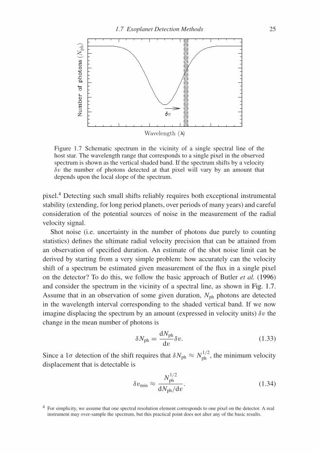
1.7 Exoplanet Detection Methods 25
Wavelength ( )
(Nph
)
v
Figure 1.7 Schematic spectrum in the vicinity of a single spectral line of thehost star. The wavelength range that corresponds to a single pixel in the observedspectrum is shown as the vertical shaded band. If the spectrum shifts by a velocityδv the number of photons detected at that pixel will vary by an amount thatdepends upon the local slope of the spectrum.
pixel.4 Detecting such small shifts reliably requires both exceptional instrumentalstability (extending, for long period planets, over periods of many years) and carefulconsideration of the potential sources of noise in the measurement of the radialvelocity signal.
Shot noise (i.e. uncertainty in the number of photons due purely to countingstatistics) defines the ultimate radial velocity precision that can be attained froman observation of specified duration. An estimate of the shot noise limit can bederived by starting from a very simple problem: how accurately can the velocityshift of a spectrum be estimated given measurement of the flux in a single pixelon the detector? To do this, we follow the basic approach of Butler et al. (1996)and consider the spectrum in the vicinity of a spectral line, as shown in Fig. 1.7.Assume that in an observation of some given duration, Nph photons are detectedin the wavelength interval corresponding to the shaded vertical band. If we nowimagine displacing the spectrum by an amount (expressed in velocity units) δv thechange in the mean number of photons is
δNph = dNph
dvδv. (1.33)
Since a 1σ detection of the shift requires that δNph ≈ N1/2ph , the minimum velocity
displacement that is detectable is
δvmin ≈ N1/2ph
dNph/dv. (1.34)
4 For simplicity, we assume that one spectral resolution element corresponds to one pixel on the detector. A realinstrument may over-sample the spectrum, but this practical point does not alter any of the basic results.
26 Observations of Planetary Systems
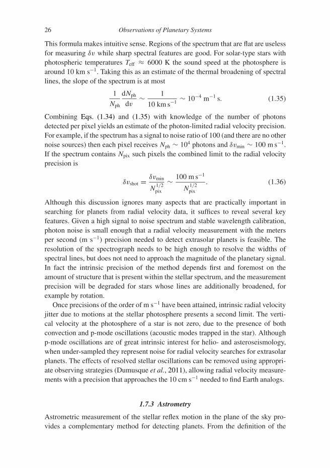
This formula makes intuitive sense. Regions of the spectrum that are flat are uselessfor measuring δv while sharp spectral features are good. For solar-type stars withphotospheric temperatures Teff ≈ 6000 K the sound speed at the photosphere isaround 10 km s−1. Taking this as an estimate of the thermal broadening of spectrallines, the slope of the spectrum is at most
1
Nph
dNph
dv∼ 1
10 km s−1 ∼ 10−4 m−1 s. (1.35)
Combining Eqs. (1.34) and (1.35) with knowledge of the number of photonsdetected per pixel yields an estimate of the photon-limited radial velocity precision.For example, if the spectrum has a signal to noise ratio of 100 (and there are no othernoise sources) then each pixel receives Nph ∼ 104 photons and δvmin ∼ 100 m s−1.If the spectrum contains Npix such pixels the combined limit to the radial velocityprecision is
δvshot = δvmin
N1/2pix
∼ 100 m s−1
N1/2pix
. (1.36)
Although this discussion ignores many aspects that are practically important insearching for planets from radial velocity data, it suffices to reveal several keyfeatures. Given a high signal to noise spectrum and stable wavelength calibration,photon noise is small enough that a radial velocity measurement with the metersper second (m s−1) precision needed to detect extrasolar planets is feasible. Theresolution of the spectrograph needs to be high enough to resolve the widths ofspectral lines, but does not need to approach the magnitude of the planetary signal.In fact the intrinsic precision of the method depends first and foremost on theamount of structure that is present within the stellar spectrum, and the measurementprecision will be degraded for stars whose lines are additionally broadened, forexample by rotation.
Once precisions of the order of m s−1 have been attained, intrinsic radial velocityjitter due to motions at the stellar photosphere presents a second limit. The verti-cal velocity at the photosphere of a star is not zero, due to the presence of bothconvection and p-mode oscillations (acoustic modes trapped in the star). Althoughp-mode oscillations are of great intrinsic interest for helio- and asteroseismology,when under-sampled they represent noise for radial velocity searches for extrasolarplanets. The effects of resolved stellar oscillations can be removed using appropri-ate observing strategies (Dumusque et al., 2011), allowing radial velocity measure-ments with a precision that approaches the 10 cm s−1 needed to find Earth analogs.
1.7.3 Astrometry
Astrometric measurement of the stellar reflex motion in the plane of the sky pro-vides a complementary method for detecting planets. From the definition of the
1.7 Exoplanet Detection Methods 27
center of mass, the physical size of the stellar orbit is related to the planetarysemi-major axis via a∗ = (Mp/M∗)a. For a star at distance d from the Earth theangular displacement of the stellar photo-center during the course of an orbit has acharacteristic scale,
θ =(
Mp
M∗
)a
d. (1.37)
Unlike radial velocity searches, which are biased toward detecting short periodplanets, astrometry favors large semi-major axes. A further difference is thatastrometry measures two independent components of the stellar motion (versusa single component via radial velocity measurements), and this yields moreconstraints on the orbit. As a result there is no sin i ambiguity and all of theimportant planetary properties can be directly measured. Numerically the size ofthe signal is
θ = 5 × 10⁻⁴
(Mp
MJ
)(M∗M�
)−1 ( a
5 AU
)(d
10 pc
)−1
arcsec. (1.38)
Even though the parameters adopted here are rather optimistic this is still a verysmall displacement, and none of the planets found in the first decade of discoverywere identified this way. In principle, however, there are no fundamental obstaclesto achieving astrometric accuracies of 1–10 μarcsec, which is good enough to detecta wide range of hypothetical planets. A 10M⊕ planet at 1 AU, for example, yieldsan astrometric signature of 3 μarcsec at d = 10 pc.
1.7.4 Transits
A planet whose orbit causes it to transit the stellar disk can be detected by mon-itoring the stellar flux for periodic dips. At the most basic level transit eventscan be characterized in terms of their depth (the fraction of the stellar flux thatis obscured), duration, and probability of being observed by a randomly orientedexternal observer. These quantities are readily estimated. The depth or amplitude ofthe transit signal is independent of the distance between the planet and the star, andprovides a measure of the relative size of the two bodies. If a planet of radius Rp
occults a star of radius R∗, with the geometry shown in Fig. 1.8, the fractionaldecrement in the stellar flux during the transit (assuming a uniform brightnessstellar disk) is just
f =(
Rp
R∗
)2
. (1.39)
Gas giant planets have a rather flat mass–radius relation, so it is reasonable to useJupiter’s radius RJ = 7.142 × 109 cm as a proxy for all giant planet transits. The
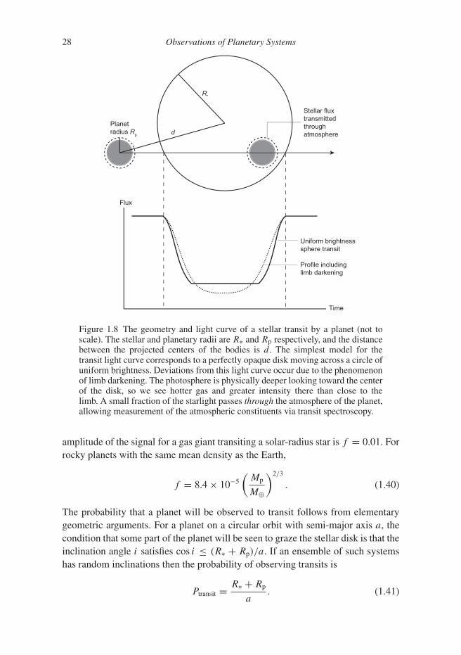
28 Observations of Planetary Systems
R*
dPlanet radius Rp
Flux
Time
Uniform brightness sphere transit
Profile includinglimb darkening
Stellar fluxtransmittedthrough atmosphere
Figure 1.8 The geometry and light curve of a stellar transit by a planet (not toscale). The stellar and planetary radii are R∗ and Rp respectively, and the distancebetween the projected centers of the bodies is d. The simplest model for thetransit light curve corresponds to a perfectly opaque disk moving across a circle ofuniform brightness. Deviations from this light curve occur due to the phenomenonof limb darkening. The photosphere is physically deeper looking toward the centerof the disk, so we see hotter gas and greater intensity there than close to thelimb. A small fraction of the starlight passes through the atmosphere of the planet,allowing measurement of the atmospheric constituents via transit spectroscopy.
amplitude of the signal for a gas giant transiting a solar-radius star is f = 0.01. Forrocky planets with the same mean density as the Earth,
f = 8.4 × 10⁻⁵
(Mp
M⊕
)2/3
. (1.40)
The probability that a planet will be observed to transit follows from elementarygeometric arguments. For a planet on a circular orbit with semi-major axis a, thecondition that some part of the planet will be seen to graze the stellar disk is that theinclination angle i satisfies cos i ≤ (R∗ + Rp)/a. If an ensemble of such systemshas random inclinations then the probability of observing transits is
Ptransit = R∗ + Rp
a. (1.41)
1.7 Exoplanet Detection Methods 29
For a planet similar to the Earth, the probability is Ptransit ≈ 5 × 10⁻³. If thegeometry is favorable for observing transits, their maximum duration is roughly2R∗/vK. More accurately (Quirrenbach, 2006),
ttransit = P
πsin−1
(√(R∗ + Rp)2 − a2 cos2 i
a
), (1.42)
where P is the orbital period. A planet similar to the Earth whose orbit is seenedge-on (i = 90◦) transits its host star for 13 hours. Combining this result withthe transit probability, one finds that if every star were to host an Earth-like planet,about 1 in 105 stars would be being transited at any given time.
The predicted light curve for an idealized (noise-free) planetary transit can becomputed using various approximate or empirical models for the brightness dis-tribution of the stellar disk. The simplest model treats the planet as a perfectlyocculting disk passing across the face of a star whose brightness or specific intensityis everywhere constant. Following Mandel and Agol (2002) we set up the problemas shown in Fig. 1.8. The planet and star have radii Rp and R∗ respectively, and theinstantaneous separation of the centers of the two bodies is d. We define auxiliaryvariables z ≡ d/R∗ and p = Rp/R∗. In terms of these variables the fractionaldecrement f is given as
f (p,z) =
⎧⎪⎪⎪⎪⎪⎨⎪⎪⎪⎪⎪⎩
0 1 + p < z,
1π
[p2κ0 + κ1 −
√4z2−(1+z2−p2)2
4
]|1 − p| < z ≤ 1 + p,
p2 z ≤ 1 − p,
1 z ≤ p − 1.
(1.43)
In these expressions,
κ0 = cos−1
[p2 + z2 − 1
2pz
], (1.44)
κ1 = cos−1
[1 − p2 + z2
2z
]. (1.45)
Unfortunately this model, which is simple enough to be written entirely in termsof elementary functions, is not very realistic. Real transit light curves do not showthe perfectly flat bottoms with f = p2 that would be predicted for a black diskcrossing a star of uniform brightness. The problem is limb darkening. The line ofsight to the star is perpendicular to the stellar surface at the center of the disk, butincreasingly tangential as we move toward the limb. As a consequence, photonscoming from the center of the star last scattered, on average, at a greater physicaldepth than those coming from near the limb. Greater physical depth corresponds toa higher temperature, so the central brightness is greatest and the limb regions arerelatively darkened. There is no exact first principles description of limb darkening,
30 Observations of Planetary Systems
but a variety of empirical laws fit observational data well. Mandel and Agol (2002)provide more complex but still analytic light curves for some of these laws.
Noise sources for transit searches include photon shot noise, stellar variability(including a contribution from the asteroseismic modes), and, for ground-basedexperiments, atmospheric fluctuations. For stars of roughly solar radii ground-basedexperiments are an efficient means of finding planets with Rp � RJ, while smallerplanets with Rp � R⊕ are only detectable given the lower noise levels attainablefrom space. Ground-based surveys are sensitive to roughly Earth-radius planetsaround M-dwarfs, which are physically much smaller. An example is GJ 1132b,a 1.2 R⊕ planet orbiting a 0.18 M� star that was discovered from the ground(Berta-Thompson et al., 2015). In addition to these true noise sources all transitsurveys have to contend with false positives that are caused by planetary transit-like signals of alternate astronomical origin. A stellar eclipsing binary, for example,may source a signal that looks like a planet if its light is diluted by the presence ofa third unresolved star within the photometric aperture. A combination of follow-up observations, yielding radial velocity or higher spatial resolution adaptive opticsdata, and statistical arguments are used to discriminate between such imposters andtrue planets.
Detection of repeated planetary transit signals provides an immediate measureof the orbital period, and of the ratio between the physical size of the planet relativeto the star. In cases where multiple planets are observed to transit the same star,gravitational perturbations between the planets lead to small changes in the timeat which transits occur. When detectable these Transit-Timing Variations (TTVs)provide constraints and in some cases measurements of the planetary masses (Agolet al., 2005; Holman & Murray, 2005; Holczer et al., 2016). Planetary massescan also be determined for systems in which transit data are supplemented byradial velocity measurements. In this case knowledge of the inclination removesthe usual sin i uncertainty in the mass. Time-resolved measurement of the radialvelocity signal during the transit also opens up the possibility of detecting theRossiter–McLaughlin effect (originally discussed in the context of eclipsing stellarbinaries; Rossiter, 1924; McLaughlin, 1924). The Rossiter–McLaughlin effect isa perturbation to the apparent stellar radial velocity that is caused by the fact thatwhen a planet transits across the face of a rotating star, it obscures portions of thestellar photosphere that are either redshifted or blueshifted relative to the whole-disk average. Figure 1.9 illustrates the principle. Detection of the effect allows fora measurement of the projected obliquity, on the plane of the sky, between thestellar and orbital angular momentum vectors. This, in turn, informs and constrainstheoretical models for the origin of planets in short-period orbits.
Transiting systems are also a rich source of informative data on planetary atmo-spheres. In some cases one can detect the secondary eclipse when the planet movesbehind the star, and in others it is possible to measure the out-of-eclipse phase mod-ulation as the planet orbits. Depending upon the wavelength of the observations,

1.7 Exoplanet Detection Methods 31
Ω
---
+++
------
++++++
-------
+++++++
Ω
---
+++
------
++++++
-------
+++++++
Ω
---
+++
------
++++++
-------
+++++++
+- +
+++
-+
++
Planet orbit alignedwith stellar spin
Planet orbit misalignedwith stellar spin
Retrograde planet orbit
Blueshiftedstellar photosphere
Redshiftedstellar photosphere
Ste
llar r
adia
l vel
ocity
Ste
llar r
adia
l vel
ocity
Ste
llar r
adia
l vel
ocity
t
t
t
Planet first blocks blueshiftedphotosphere, leading to apparent stellar redshift
Figure 1.9 Illustration of the Rossiter–McLaughlin effect. Selective obscurationof the photosphere of a rotating star introduces a time-dependent perturbationto the measured radial velocity signal as a planet transits the star. The form ofthe perturbation depends upon whether the planet first blocks a redshifted orblueshifted piece of photosphere, and hence probes for misalignment between thestellar and orbital angular momentum vectors.
data of this type can constrain the albedo of the planet or the size of the differencebetween the temperature of the day side and that of the night side. Even morepowerful are observations of the apparent size of the planet at different wavelengths,due to light that passes through the atmosphere at the planet’s limb. This is a smalleffect. For a planet whose atmosphere has temperature T , mean molecular weightμ, and surface gravity g, the exponential scale-height is
Hp = kBT
μg, (1.46)
where kB is the Boltzmann constant. Suppose that we observe a planet at twowavelengths, one where the atmosphere is entirely transparent (so that the apparentplanetary size is given by that of the solid surface) and one where an atmosphericabsorber is optically thick up to n scale-heights above the surface. The transit depthmeasured at the two wavelengths will differ by an amount
δf = (Rp + nHp)2
R2∗− R2
p
R2∗
� 2nRpHp
R2∗. (1.47)

32 Observations of Planetary Systems
For an Earth analog with Hp = 8 km orbiting a solar-type star δf ∼ 2 × 10⁻⁷,and detecting this effect is close to 1000 times harder than simply seeing the transititself. Larger signals, which are detectable today, occur for larger or hotter planets,and for those orbiting smaller stars. In these cases measurement of the apparentplanetary radius as a function of observing wavelength provides a handle on theatmospheric composition.
1.7.5 Gravitational Microlensing
Gravitational microlensing is a powerful method for detecting extrasolar planetsthat is based upon indirectly detecting the gravitational deflection of light thatpasses through the planetary system from a background source. The foundationsof the method were laid by Einstein, who derived the general relativistic result forlight bending by gravitating objects. A photon that passes a star of mass M∗ withimpact parameter b is deflected by an angle
α = 4GM∗bc2
. (1.48)
If two stars lie at different distances along the same line of sight, consideration ofthe geometry illustrated in Fig. 1.10 implies that the image of the background star(the “source”) is distorted by the deflection introduced by the foreground star (the“lens”) into a ring. Writing the distance between the observer and the lens as dL,the observer–source distance as dS, and the lens–source distance as dLS, the angularradius of the so-called Einstein ring is
θE = 2
c
√GM∗dLS
dLdS. (1.49)
dLdLS
dS
Lens plane
Sourceplane
qE
α
Obs
erve
r
Figure 1.10 Microlensing geometry. Light from a background star is deflected bya small angle α when it passes a foreground star of mass M∗. If the alignmentbetween the foreground and background star is perfect, then by symmetry theobserver sees the image of the background star distorted into a circular Einsteinring around the foreground star. The ring has an angular radius θE. When lensingis used as a tool to detect planets, the distances involved are such that the ring isunresolved. The observable is the change in brightness of the background star asthe two stars first align, and then move apart.

1.7 Exoplanet Detection Methods 33
If the alignment between the source and the lens is nearly but not quite perfect,the axial symmetry is broken and the source is lensed into multiple images whoseangular separation is also of the order of θE.
For planet detection, a typical configuration of interest observationally is thatwhere the source star lies in the Galactic bulge (dS = 8 kpc) and the lens star isin the disk (dL ≈ 4 kpc). The Einstein ring radius for a solar mass lens with theseparameters is θE ∼ 10−3 arcsec, so the multiple images cannot be spatially resolved.A property of lensing, however, is that it conserves surface brightness. The area ofthe lensed image is greater than it would have been in the absence of lensing, andhence the flux from the lensed images exceeds that of the unlensed star. This meansthat if the alignment between the source and the lens varies with time, monitoring ofthe light curve of the source star can detect unresolved lensing via the time-variablemagnification caused by lensing. Light curves in which a single disk star lensesa background star are smooth, symmetric about the peak, and magnify the sourceachromatically. If the proper motion of the lens relative to that of the source is μ,the characteristic time scale of the lensing event is tE = θE/μ. For events toward theGalactic bulge this time scale is about a month, scaling with the lens mass as
√M∗.
Microlensing light curves are altered when the lens star is part of a binary. Forstar–planet systems in which the mass ratio q = Mp/M∗ 1 the conceptuallysimplest case to consider is when the planet orbits close to the physical radiusof the Einstein ring at the distance of the lens. If one of the multiple images ofthe source passes close to the planet during the lensing event the planet’s gravityintroduces an additional perturbation to the light curve. To an order of magnitude,the time scale of the perturbation is just tp ∼ q1/2tE, while the probability that thegeometry will be such that a perturbation occurs is P ∼ Aq1/2, where A is themagnification of the source at the moment when the image passes near the planet.A second channel for planet detection occurs in rare high magnification events,during which planets close to the Einstein ring modify the light curve near peakregardless of their orbital position. This channel is valuable observationally sincehigh magnification events can be anticipated based on photometric observationsmade well before the peak, allowing for detailed monitoring of those events thatare most favorable for detecting planets.
Determining the properties of planets from the analysis of microlensing lightcurves is a difficult inverse problem, but the above discussion is enough to explainthe attractive aspects of the method. First, the physical radius of the Einstein ringfor disk stars lensing background stars in the Galactic bulge corresponds to a fewAU. Lensing is therefore well suited to detect planets at relatively large orbitalradii (roughly corresponding to the location of the snow line in the Solar System)which are challenging to detect via radial velocity or transit methods. Second, theweak
√MP dependence of the time scale on planet mass allows for a wide range of
planets to be detected. In particular, Jupiter mass planets yield a perturbation timescale of around a day, while Earth mass planets have a characteristic time scaleof about an hour. Both time scales are quite accessible observationally. Moreover,
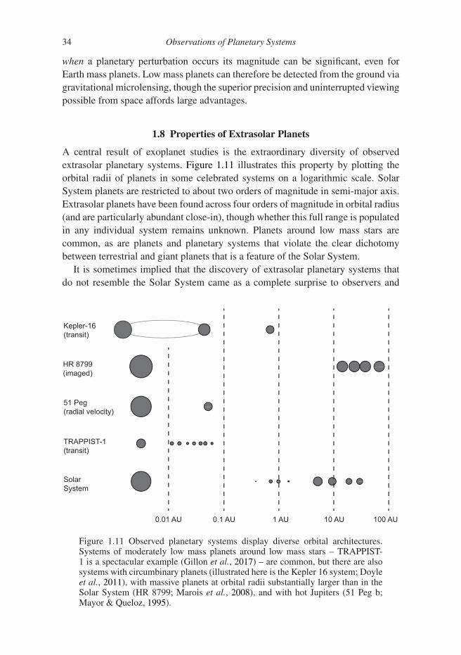
34 Observations of Planetary Systems
when a planetary perturbation occurs its magnitude can be significant, even forEarth mass planets. Low mass planets can therefore be detected from the ground viagravitational microlensing, though the superior precision and uninterrupted viewingpossible from space affords large advantages.
1.8 Properties of Extrasolar Planets
A central result of exoplanet studies is the extraordinary diversity of observedextrasolar planetary systems. Figure 1.11 illustrates this property by plotting theorbital radii of planets in some celebrated systems on a logarithmic scale. SolarSystem planets are restricted to about two orders of magnitude in semi-major axis.Extrasolar planets have been found across four orders of magnitude in orbital radius(and are particularly abundant close-in), though whether this full range is populatedin any individual system remains unknown. Planets around low mass stars arecommon, as are planets and planetary systems that violate the clear dichotomybetween terrestrial and giant planets that is a feature of the Solar System.
It is sometimes implied that the discovery of extrasolar planetary systems thatdo not resemble the Solar System came as a complete surprise to observers and
0.01 AU 0.1 AU 1 AU 10 AU 100 AU
SolarSystem
TRAPPIST-1(transit)
51 Peg(radial velocity)
HR 8799(imaged)
Kepler-16(transit)
Figure 1.11 Observed planetary systems display diverse orbital architectures.Systems of moderately low mass planets around low mass stars – TRAPPIST-1 is a spectacular example (Gillon et al., 2017) – are common, but there are alsosystems with circumbinary planets (illustrated here is the Kepler 16 system; Doyleet al., 2011), with massive planets at orbital radii substantially larger than in theSolar System (HR 8799; Marois et al., 2008), and with hot Jupiters (51 Peg b;Mayor & Queloz, 1995).

1.8 Properties of Extrasolar Planets 35
theorists alike. This is an over-statement. Otto Struve, in proposing a programof high-precision radial velocity measurements, suggested that it is “not unrea-sonable that a planet might exist at a distance of 0.02 AU” (Struve, 1952), andtheorists expected that planets ought to be common (e.g. Wetherill, 1991) and iden-tified in advance some of the mechanisms that lead to orbital migration (Goldreich& Tremaine, 1980). It is the extent of the differences between the Solar Systemand many extrasolar planetary systems that constitutes a genuine surprise. It hasprompted both a re-evaluation of the effects of previously known planet formationprocesses, and a search for new ones.
1.8.1 Parameter Space of Detections
Figure 1.12 shows the distribution of semi-major axes for a sample of extrasolarplanets with known masses. This plot, and most like it, is neither complete norunbiased, and it omits most transit-detected planets as these often lack mass esti-mates. It suffices, however, to illustrate the main populations of known extrasolarplanets.
EarthVenus
Mars
Jupiter
Saturn
Uranus
Neptune
10
1
0.1
0.01
0.001
0.01 0.1 1 10 100Semi-major axis (AU)
Pla
net m
ass
(MJ)
hotJupiters
Figure 1.12 The distribution of a sample of known extrasolar planets in semi-major axis and planet mass (either Mp or Mp sin i, depending upon the availableobservations). Selected Solar System planets are shown as the open squares. Datafrom the NASA Exoplanet Archive.

36 Observations of Planetary Systems
In the realm of giant planets with masses equal to or larger than Saturn, a popu-lation of “warm” and “cold” Jupiters extends from a few tenths of an AU out to atleast Jupiter’s orbital radius. Knowledge of the true outer extent of this population iscurrently limited by selection effects. The masses of extrasolar giant planets rangeup to the deuterium burning limit (an order of magnitude larger than in the SolarSystem), but there are relatively few brown dwarfs with AU-scale orbits aroundsolar mass stars, a property known as the “brown dwarf desert.” Statistical studiesshow that giant planets with orbital periods P < few yr orbit approximately 10%of Sun-like stars. Over the observed range of orbital radii the probability density isroughly uniform in log P . Low mass giants are more common than high mass ones.Cumming et al. (2008) estimated that dNp/d ln M ∝ Mα with α � −0.3 ± 0.2 forthis population.
Closer in the “hot Jupiters” have clearly distinct physical and dynamical prop-erties, and possibly a different formation history, than their colder brethren. Theseplanets orbit within about 0.1 AU of their hosts, and have correspondingly higheffective temperatures. They have near circular orbits and are expected to be intidally synchronized rotation states. Hot Jupiters are present around approximately1% of solar-type stars, and are less common around M dwarfs (Dawson & John-son, 2018).
Lower mass planets, although under-represented in Fig. 1.12, are substantiallymore common. Statistics of this population were derived from the results of theKepler mission, which monitored ≈150 000 stars of spectral type FGKM for tran-sits for 4 years. Roughly half of Sun-like stars have planets with radii 1−4 R⊕ withorbital periods P ≤ 1 yr. Closely spaced systems with multiple planets in theserelatively short-period orbits are common (Winn & Fabrycky, 2015).
A small number of stars are known to host massive planets with orbital radiisubstantially larger than any of the Solar System’s giant planets. An example isHR 8799, a 1.5 M⊕ star that is still young enough to have a debris disk. HR 8799has at least four planets, with masses of ∼5–10 MJ and orbital radii between 15 and70 AU (Marois et al., 2008).
Important parts of the parameter space of possible planetary systems remainpoorly surveyed. Knowledge of the abundance of planets with masses or radiicomparable to the Earth is extremely limited beyond ≈1 AU, while beyond 10 AUinformation even on giant planets is scant. A full picture of the architecture oftypical extrasolar planetary systems is also lacking. At the time of writing mostknown close-in low mass planets were discovered using Kepler data, and orbitrelatively faint stars that are hard to monitor for long-period radial velocity signals.As a consequence, knowledge of the relationship between low mass and giantplanets in extrasolar planetary systems is more limited than one might expectgiven the amount of good data on each individual population. Basic questions,such as the average number of planets that orbit stars of different masses, remainopen.
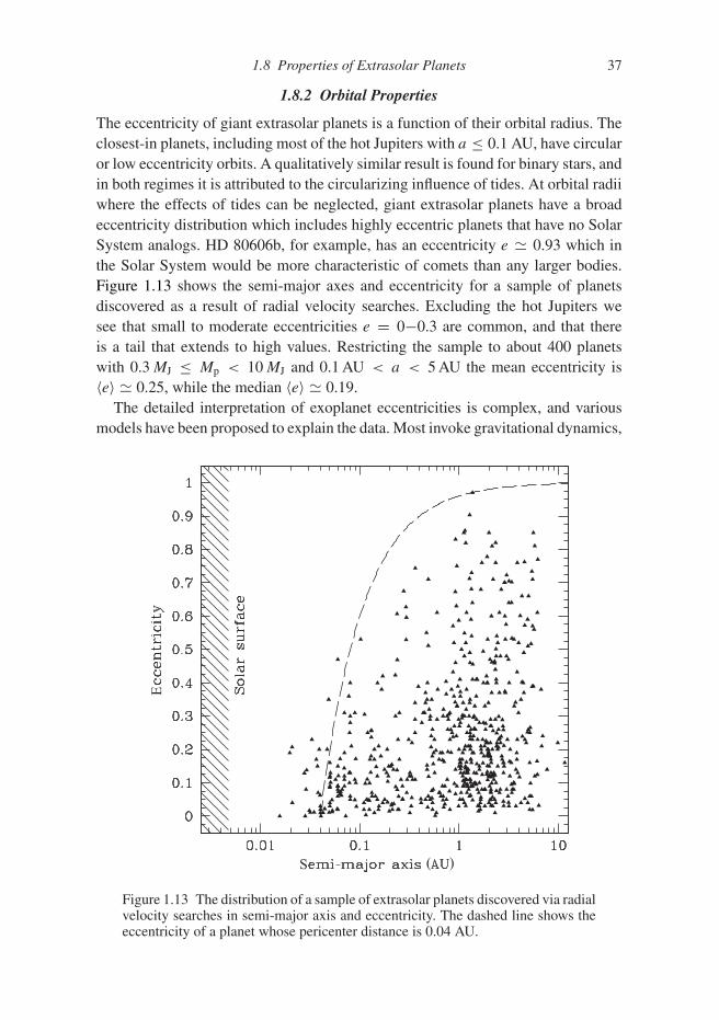
1.8 Properties of Extrasolar Planets 37
1.8.2 Orbital Properties
The eccentricity of giant extrasolar planets is a function of their orbital radius. Theclosest-in planets, including most of the hot Jupiters with a ≤ 0.1 AU, have circularor low eccentricity orbits. A qualitatively similar result is found for binary stars, andin both regimes it is attributed to the circularizing influence of tides. At orbital radiiwhere the effects of tides can be neglected, giant extrasolar planets have a broadeccentricity distribution which includes highly eccentric planets that have no SolarSystem analogs. HD 80606b, for example, has an eccentricity e � 0.93 which inthe Solar System would be more characteristic of comets than any larger bodies.Figure 1.13 shows the semi-major axes and eccentricity for a sample of planetsdiscovered as a result of radial velocity searches. Excluding the hot Jupiters wesee that small to moderate eccentricities e = 0−0.3 are common, and that thereis a tail that extends to high values. Restricting the sample to about 400 planetswith 0.3 MJ ≤ Mp < 10 MJ and 0.1 AU < a < 5 AU the mean eccentricity is〈e〉 � 0.25, while the median 〈e〉 � 0.19.
The detailed interpretation of exoplanet eccentricities is complex, and variousmodels have been proposed to explain the data. Most invoke gravitational dynamics,
E
S ( )
Figure 1.13 The distribution of a sample of extrasolar planets discovered via radialvelocity searches in semi-major axis and eccentricity. The dashed line shows theeccentricity of a planet whose pericenter distance is 0.04 AU.

38 Observations of Planetary Systems
P(
)
T ( )
Figure 1.14 The sky-projected angle between the stellar spin axis and the orbitalplane of close-in massive planets. The sample includes hot Jupiters with orbitalperiod P < 7 days, masses between 0.3 and 3 MJ, and quoted measurement errorsof less than 10◦ (data from Wright et al., 2011a).
taking place after the main phase of planet formation, to excite the eccentricity ofinitially near-circular giant planets. The observed distribution may also be affectedby interactions (also mediated by gravity) between planets and gas that occur beforeor during the dispersal of the protoplanetary disk.
Measurements of the Rossiter–McLaughlin effect (Fig. 1.9) provide a constrainton how well planetary orbits align with the equators of their host stars. The observ-able quantity is not the misalignment itself but rather the projected obliquity, that isthe angle between the vectors describing the orbit and the stellar spin projected onthe sky plane. Figure 1.14 shows measurements of the projected obliquity for a sam-ple of hot Jupiters orbiting stars of varying effective temperature Teff. A subset ofhot Jupiters have high projected obliquities, which implies that some giant planetsorbit their stars in highly tilted, polar, or even retrograde orbits. The observeddistribution has a striking dependence on the stellar effective temperature. Low pro-jected obliquities are the norm for Teff
<∼ 6100 K, while a wide range of obliquitiescharacterize hot Jupiters around hotter stars (Winn et al., 2010).
A small number of dynamical processes, including the Kozai–Lidov effect whichwe will discuss in Chapter 7, are able to tilt the orbits of planets that form initiallyin the plane defined by the stellar spin. They were fingered as prime suspects assoon as the first examples of misaligned hot Jupiters were identified. Alternatively,the disk plane itself could be tilted away from the equatorial one in some fractionof systems, leading to a primordial origin for the misalignments (Bate et al., 2010;Batygin, 2012). In either case the fact that the threshold in effective temperaturecoincides with known structural differences in stars suggests that stellar rotationand tidal dissipation play a role in shaping the late-time distribution.
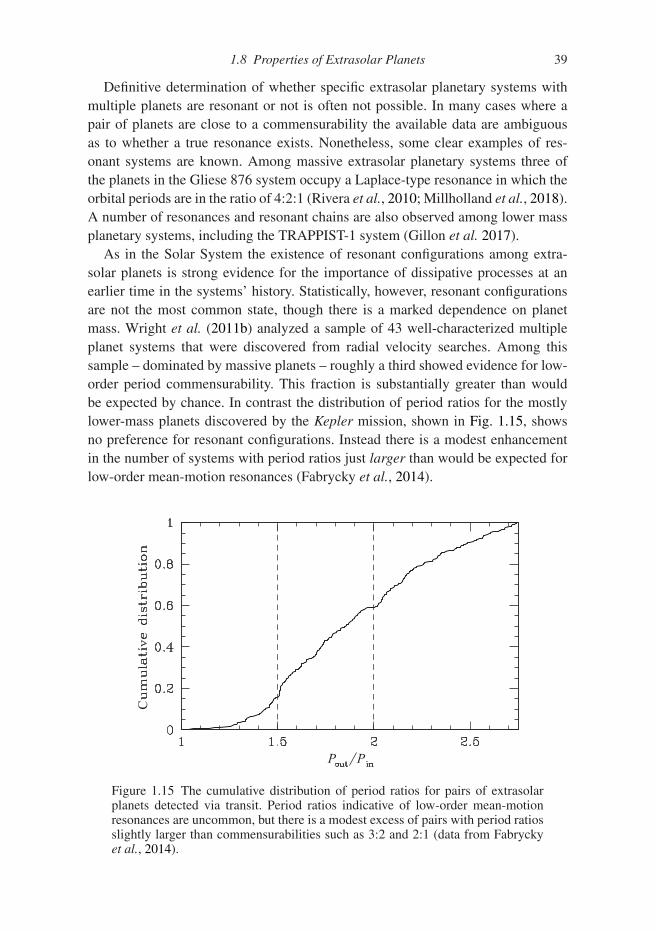
1.8 Properties of Extrasolar Planets 39
Definitive determination of whether specific extrasolar planetary systems withmultiple planets are resonant or not is often not possible. In many cases where apair of planets are close to a commensurability the available data are ambiguousas to whether a true resonance exists. Nonetheless, some clear examples of res-onant systems are known. Among massive extrasolar planetary systems three ofthe planets in the Gliese 876 system occupy a Laplace-type resonance in which theorbital periods are in the ratio of 4:2:1 (Rivera et al., 2010; Millholland et al., 2018).A number of resonances and resonant chains are also observed among lower massplanetary systems, including the TRAPPIST-1 system (Gillon et al. 2017).
As in the Solar System the existence of resonant configurations among extra-solar planets is strong evidence for the importance of dissipative processes at anearlier time in the systems’ history. Statistically, however, resonant configurationsare not the most common state, though there is a marked dependence on planetmass. Wright et al. (2011b) analyzed a sample of 43 well-characterized multipleplanet systems that were discovered from radial velocity searches. Among thissample – dominated by massive planets – roughly a third showed evidence for low-order period commensurability. This fraction is substantially greater than wouldbe expected by chance. In contrast the distribution of period ratios for the mostlylower-mass planets discovered by the Kepler mission, shown in Fig. 1.15, showsno preference for resonant configurations. Instead there is a modest enhancementin the number of systems with period ratios just larger than would be expected forlow-order mean-motion resonances (Fabrycky et al., 2014).
C
P P
Figure 1.15 The cumulative distribution of period ratios for pairs of extrasolarplanets detected via transit. Period ratios indicative of low-order mean-motionresonances are uncommon, but there is a modest excess of pairs with period ratiosslightly larger than commensurabilities such as 3:2 and 2:1 (data from Fabryckyet al., 2014).
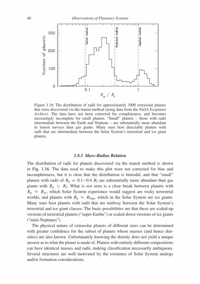
40 Observations of Planetary Systems
N
R R
Figure 1.16 The distribution of radii for approximately 3000 extrasolar planetsthat were discovered via the transit method (using data from the NASA ExoplanetArchive). The data have not been corrected for completeness, and becomesincreasingly incomplete for small planets. “Small” planets – those with radiiintermediate between the Earth and Neptune – are substantially more abundantin transit surveys than gas giants. Many stars host detectable planets withradii that are intermediate between the Solar System’s terrestrial and ice giantplanets.
1.8.3 Mass–Radius Relation
The distribution of radii for planets discovered via the transit method is shownin Fig. 1.16. The data used to make this plot were not corrected for bias andincompleteness, but it is clear that the distribution is bimodal, and that “small”planets with radii of Rp = 0.1−0.4 RJ are substantially more abundant than gasgiants with Rp � RJ. What is not seen is a clear break between planets withRp ≈ R⊕, which Solar System experience would suggest are rocky terrestrialworlds, and planets with Rp ≈ RNep, which in the Solar System are ice giants.Many stars host planets with radii that are midway between the Solar System’sterrestrial and ice giant classes. The basic possibilities are that these are scaled-upversions of terrestrial planets (“super-Earths”) or scaled-down versions of ice giants(“mini-Neptunes”).
The physical nature of extrasolar planets of different sizes can be determinedwith greater confidence for the subset of planets whose masses (and hence den-sities) are also known. Unfortunately knowing the density does not yield a uniqueanswer as to what the planet is made of. Planets with entirely different compositionscan have identical masses and radii, making classification necessarily ambiguous.Several structures are well motivated by the existence of Solar System analogsand/or formation considerations.

1.8 Properties of Extrasolar Planets 41
• Gas giants with masses roughly in the range between MSat and 13 MJ. Theoreticalmodels of gas giant structure show that the predicted radius is a weak functionof mass, so to leading order gas giants ought to have Rp � RJ. At the next orderof approximation the radius is a decreasing function of the total mass of heavyelements within the planet, independent of whether that material is concentratedin a core or dispersed throughout the envelope.
• Rocky planets. There is no clear lower limit to the mass of rocky (or icy) worlds,though bodies smaller than a few hundred km in size are typically irregular inshape and fall into the class of minor bodies. There is also no absolute upperlimit, though once we reach masses of 5–10 M⊕ capture of an envelope denseenough to increase the radius measured via transit becomes increasingly likely.Zeng et al. (2016) provide a semi-empirical model for the mass-radius relation ofbroadly Earth-like planets,
Rp = (1.07 − 0.21fcore)
(Mp
M⊕
)1/3.7
R⊕, (1.50)
valid for the range between 1 and 8 Earth masses. In this expression fcore is thecore mass fraction (for the Earth fcore � 0.33). Smaller radii are possible foriron-rich planets (Mercury-like and super-Mercury worlds), with the minimumphysically plausible radii being attained for objects made up of 100% Fe.
• Low mass core/envelope planets. A variety of structures are possible withinthe generic class of a rocky or icy core (typically of a few to about ten M⊕)surrounded by a sub-dominant gaseous envelope. End members are “gas dwarfs,”where the envelope is made up of hydrogen and helium, and objects where theenvelope is heavily enriched with water and other species such as NH3 and CH4.Planets with these structural features would be seen as low density objects withmasses of a few to about ten Earth masses.
• Water worlds. The high predicted abundance of water beyond the snow line inprotoplanetary disks opens up the possibility of planets with a water dominatedbulk composition. Such planets have a mass–radius relation that is similar torocky planets, but 30–40% larger in size.
Figure 1.17 shows the observed masses and radii of a sample of extrasolar planetsfor which both quantities have been measured with moderate to good precision.Among giant planets the weak predicted dependence of radius on mass is clearlyevident. A small number of giant planets have anomalously small radii, indicativeof a large bulk heavy element abundance. Among the hot Jupiters, many planetshave anomalously large radii, exceeding in some cases the prediction for a planetthat lacks a significant mass of heavy elements. These radius anomalies correlatewith the incident stellar irradiation, giving support to the hypothesis that somefraction of the incident stellar energy finds its way into the planets’ convectivezones. Energy input into the convection zone is known to stall contraction or inflate

42 Observations of Planetary Systems
R
MM
R
Figure 1.17 The distribution of a sample of extrasolar planets with well-determined mass and radius estimates.
giant planets, though the mechanism that injects stellar energy deep into the planetremains unclear.
Mass and radius data for smaller planets are sparser, especially for planets withmasses similar to or smaller than that of the Earth. The evidence is consistent withthe idea that many planets with Rp
<∼ 1.5 R⊕ are rocky super-Earths, while largerplanets have a range of radii that reflect variations in the amount of gas within theirenvelopes (Rogers, 2015). Not very much is known about the detailed compositionof envelopes in the mini-Neptune size range, nor can it be excluded that someobserved planets have water dominated compositions.
1.8.4 Host Properties
Important constraints on planet formation models come from the observation thatthe abundance of planets correlates with properties of the host star. A key obser-vation was the discovery by Debra Fischer and Jeff Valenti that the fraction ofstars with observed giant planets increases with the metal abundance measuredspectrosopically in the stellar photosphere (Fischer & Valenti, 2005). Figure 1.18shows an updated version of this correlation (Sousa et al., 2011). For planets (and
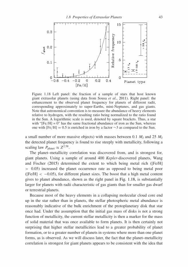
1.8 Properties of Extrasolar Planets 43
f
R
P
R
R
R
Figure 1.18 Left panel: the fraction of a sample of stars that host knowngiant extrasolar planets (using data from Sousa et al., 2011). Right panel: theenhancement to the observed planet frequency for planets of different radii,corresponding approximately to super-Earths, mini-Neptunes, and gas giants.Note that astronomical convention is to measure the abundance of heavy elementsrelative to hydrogen, with the resulting ratio being normalized to the ratio foundin the Sun. A logarithmic scale is used, denoted by square brackets. Thus, a starwith “[Fe/H] = 0” has the same fractional abundance of iron as the Sun, whereasone with [Fe/H] = 0.5 is enriched in iron by a factor ∼3 as compared to the Sun.
a small number of more massive objects) with masses between 0.1 MJ and 25 MJ
the detected planet frequency is found to rise steeply with metallicity, following ascaling law Pplanet ∝ Z2.58.
The planet–metallicity correlation was discovered from, and is strongest for,giant planets. Using a sample of around 400 Kepler-discovered planets, Wangand Fischer (2015) determined the extent to which being metal rich ([Fe/H]> 0.05) increased the planet occurrence rate as opposed to being metal poor([Fe/H] < −0.05), for different planet sizes. The boost that a high metal contentgives to planet abundance, shown as the right panel in Fig. 1.18, is substantiallylarger for planets with radii characteristic of gas giants than for smaller gas dwarfor terrestrial planets.
Because most of the heavy elements in a collapsing molecular cloud core endup in the star rather than in planets, the stellar photospheric metal abundance isreasonably indicative of the bulk enrichment of the protoplanetary disk that staronce had. Under the assumption that the initial gas mass of disks is not a strongfunction of metallicity, the current stellar metallicity is then a marker for the massof solid material that was once available to form planets. It is then certainly notsurprising that higher stellar metallicities lead to a greater probability of planetformation, or to a greater number of planets in systems where more than one planetforms, as is observed. As we will discuss later, the fact that the planet–metallicitycorrelation is strongest for giant planets appears to be consistent with the idea that
44 Observations of Planetary Systems
giant planet formation involves a time-limited threshold step – to form a giant planeta massive core needs to assemble in a limited period of time before the gas in theprotoplanetary disk disperses.
1.9 Habitability
Several factors appear to contribute to the hospitable environment that the Earthoffers for life. The surface temperature and pressure allow for the presence of liquidwater across much of the surface, and these conditions are maintained over time dueto geological processes (volcanism and plate tectonics) that stabilize the climate.Convective motions within the Earth’s core sustain a magnetic field, which reducesthe rate at which water is lost from the upper atmosphere due to collisions withhigh energy solar wind particles. Together with a moderate global abundance ofwater, established at early times, the low loss rate means that the current surfaceconditions – with both major oceans and large landmasses – have remained roughlyconstant over billions of years. Dynamical effects may also be important. Our largeMoon, for example, stabilizes the Earth’s obliquity against perturbations from theother planets, and the Solar System’s architecture does not lead to large excursionsin the Earth’s eccentricity.
A full accounting of the planetary conditions that are necessary and sufficientfor life to survive is not known, and it is a more difficult task still – bordering onguesswork – to enumerate the characteristics of planets where life might form inthe first place. It is therefore customary to adopt a deliberately limited definition ofthe “habitable zone” as the range of orbital distances where a planet of given mass,orbiting a star of specified mass or spectral type, can sustain liquid water on itssurface. To leading order this requires that the incident stellar flux be similar to the1360 W m−2 received by the Earth, and the steep scaling of stellar luminosity withstellar mass implies that the habitable zone has a strong dependence on host starmass. As shown in Fig. 1.19 a planet around a 0.2 M� star needs to orbit at roughlya � 0.1 AU to experience similar insolation as the Earth, while for the lowest masshydrogen-burning objects the habitable zone is at just a few hundredths of an AU.
A crude estimate of the width of the habitable zone can be obtained by ignor-ing atmospheric physics and assuming that a planet reradiates intercepted stellarradiation as a single temperature blackbody. For a planet with radius Rp, albedo A,and an orbital distance a from a star of luminosity L, the temperature given theseassumptions would be determined by
4πR2pσT 4 = L(1 − A)
4πa2πR2
p, (1.51)
where σ is the Stefan–Boltzmann constant. Identifying the outer and inner edgesof the habitable zone with the freezing and boiling points of water at the Earth’satmospheric pressure we estimate the relative width of the habitable zone to be

1.9 Habitability 45
Venuslimit
EarlyMarslimit
Runawaygreenhouse
Maximumgreenhouse
“Habitable zone”
“Habitable zone”
( )
T
F
r
MM
F
( )
Figure 1.19 Estimates of the extent of the habitable zone, where liquid watercan stably exist on the surface of a roughly Earth mass terrestrial planet. Theupper panel, based on calculations by Kopparapu et al. (2013), shows theoreticalestimates based on limiting cases of the greenhouse effect (solid lines) alongwith the extensions that follow if we assume that Mars and/or Venus wereonce but are no longer habitable (dashed lines). The width of the zone isexpressed for stars of different effective temperature Teff in terms of the incidentplanetary flux normalized to that of the Earth. The lower panels shows thesame estimates converted into orbital radii for main-sequence stars of givenmass.
aout
ain=
(273 K
373 K
)−2
≈ 1.9. (1.52)
Although the neglect of the greenhouse effect means that the temperatures predictedby Eq. (1.51) are inaccurate, this estimate of the width of the zone is not too far offfrom actual calculations.
The use of climate models to map out the extent of the habitable zone waspioneered by Kasting et al. (1993). A climate model predicts the surface tem-perature of a planet given a specified atmospheric composition and stellar radia-tion field.5 Geophysical assumptions are needed to define the limits of plausible
5 In practice, calculations of the habitable zone often use an “inverse” climate model in which the surfacetemperature is specified and the model is used to compute the stellar flux that would yield that temperature.

46 Observations of Planetary Systems
atmospheric compositions, which change over time. On the Earth the amount ofCO2 in the atmosphere is regulated by the carbonate–silicate cycle. Carbonate min-erals react with SiO2 under the high temperature conditions found in subductionzones to liberate CO2, which is vented into the atmosphere via volcanic activ-ity. Burton et al. (2013) estimate the magnitude of this source term to be about0.5 MT yr−1. Although dwarfed by current anthropogenic emissions this naturalsource of CO2, if unchecked, would significantly increase the atmospheric budgetof greenhouse gases and raise the global temperature on a time scale of the orderof a Myr. The counter-balancing sink is provided by weathering. AtmosphericCO2 reacts with rainwater to form carbonic acid, H2CO3, which dissolves silicaterocks on land. The weathering products flow into the oceans, where they ulti-mately reform carbonate minerals. Crucially, the weathering rate is an increasingfunction of the temperature, so it is possible (though not guaranteed) to reachan equilibrium state in which volcanic sources of CO2 balance the weatheringsink. In the extreme case where a planet becomes entirely ice covered (a “snow-ball Earth” state) the cessation of weathering and resulting build-up of CO2 pro-vides a mechanism to return the surface to habitability on a relatively short timescale.
The formation of calcium carbonate by living organisms in the oceans is animportant part of the Earth’s carbonate–silicate cycle, whose quantitative detailswould certainly be different on other planets. It seems reasonable, however, toassume that a qualitatively similar negative feedback loop acts to stabilize the cli-mate of terrestrial planets that, like the Earth, have active plate tectonics, a largereservoir of carbon, and substantial but not dominant amounts of water. Within thisclass of planets the limits to habitability can be identified with catastrophic failuresof climate stabilization mechanisms. As the stellar flux decreases for planets atlarger orbital distance, the expected drop in the surface temperature is partiallyoffset by the development of successively thicker CO2 atmospheres which pro-vide warming via the greenhouse effect. This stabilization fails once the atmo-sphere reaches a “maximum greenhouse” limit, beyond which CO2 starts to con-dense out and is unable to provide additional warming. Calculations by Kopparapuet al. (2013) for a solar-type star place the maximum greenhouse limit at F �0.35F0 (where F0 is the flux received by the Earth), corresponding to an orbitalradius of 1.7 AU. Moving in the other direction, a closer-in analog of the Earthcan maintain a stable but hotter climate until it reaches the “moist greenhouse”limit, when the stratosphere becomes dominated by water. Water can then be lostfrom the planet via a combination of dissociation of water molecules and escapeof the light H atoms. The time scale for water loss becomes less than the age ofthe Earth for a surface temperature of T ≈ 340 K, so this limit is more stringentthan the simple requirement that the temperature remain below the boiling pointof water. The oceans are expected to evaporate in their entirety at the “maximum

1.9 Habitability 47
greenhouse” limit, beyond which CO2 can accumulate further in the absence ofefficient sink processes. The nominal moist and runaway greenhouse limits for theSolar System are at 0.99 AU and 0.97 AU (Kopparapu et al., 2013), although thecooling effect of clouds (which are not included in these calculations) means thatthe Earth is not as close to the inner edge of the habitable zone as these estimateswould suggest.
Figure 1.19 shows how the inner and outer boundaries of the habitable zone arepredicted to scale with stellar mass. The leading order effect, which dominates theplot of aout(M∗) and ain(M∗) in the lower panel, is the scaling of stellar luminositywith mass. Smaller but still significant effects occur because of the shift of thepeak of the stellar spectrum with mass. Cooler stars emit a greater fraction of theirbolometric luminosity in the near-IR as compared to the visible, and this near-IRflux is both scattered less (Rayleigh scattering is proportional to λ−4) and absorbedbetter (by species such as H2O and CO2) by planetary atmospheres. An Earth analogaround a lower mass star would therefore have a lower albedo, and both the innerand outer edges of the habitable zone would be pushed outward. The magnitude ofthe shift, expressed in terms of the threshold flux F/F0, is about 20–25% for starsranging in mass between 0.1 M� and 1 M�.
Opportunities to assess the validity of theoretical estimates of the habitable zoneare for now extremely limited. Mars cannot sustain liquid water on its surface today,and hence is not within the habitable zone by our definition. The presence of rivervalleys and canyons on the Martian surface, however, strongly suggests that liquidwater flowed on Mars in the early history of the planet, and may have been stableuntil atmospheric loss under the low gravity conditions led to cooling. This line ofreasoning is consistent with the theoretical expectation that Mars’ orbit lies closeto the outer edge of the habitable zone. Much less can be said about the inner edgeof the habitable zone. Venus is assuredly not habitable today, but there is no directway of knowing whether the planet had liquid water at an early time when the solarluminosity was smaller. Empirically, then, the inner edge of the habitable zone liesbeyond the orbit of Venus, but could be significantly closer to the Sun than thetheoretical estimate shown in Fig. 1.19.
It is worth emphasizing again that the conventional definition of the habitablezone does not necessarily match up to the plain English meaning of habitability.Planets within the habitable zone may be inhospitable to life, for example becausethey possess vanishing quantities of water, while bodies far outside the zone couldin principle harbor habitable sub-surface oceans. (There is strong evidence forsuch reservoirs being present on both Jupiter’s moon Europa and Saturn’s moonEnceladus.) For these reasons, the habitable zone is best viewed as defining aregion of exoplanet parameter space that can reasonably be prioritized in follow-upatmospheric characterization studies focused on the identification of biomarkerssuch as oxygen.
48 Observations of Planetary Systems
1.10 Further Reading
The properties of the planets, moons, and minor bodies of the Solar System are discussedin depth in any planetary science text. A good example is Planetary Sciences byI. de Pater and J. J. Lissauer (updated second edition 2015, Cambridge: CambridgeUniversity Press).
The Handbook of Exoplanets (editors H. J. Deeg and J. A. Belmonte, 2018, Cham:Springer) includes review articles on different exoplanet detection methods alongwith analyses on the properties of the exoplanet population.
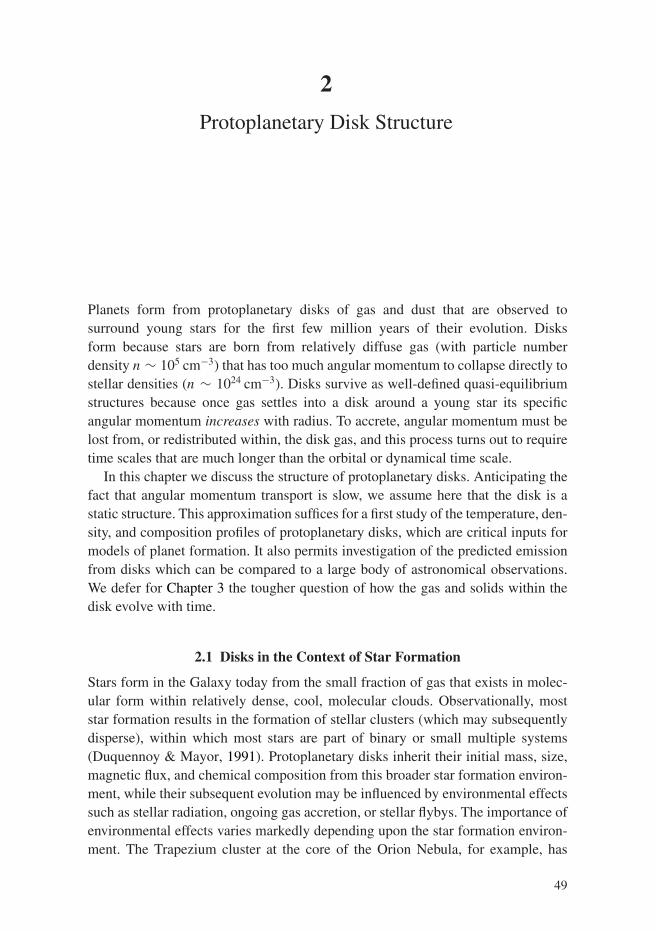
2
Protoplanetary Disk Structure
Planets form from protoplanetary disks of gas and dust that are observed tosurround young stars for the first few million years of their evolution. Disksform because stars are born from relatively diffuse gas (with particle numberdensity n ∼ 105 cm−3) that has too much angular momentum to collapse directly tostellar densities (n ∼ 1024 cm−3). Disks survive as well-defined quasi-equilibriumstructures because once gas settles into a disk around a young star its specificangular momentum increases with radius. To accrete, angular momentum must belost from, or redistributed within, the disk gas, and this process turns out to requiretime scales that are much longer than the orbital or dynamical time scale.
In this chapter we discuss the structure of protoplanetary disks. Anticipating thefact that angular momentum transport is slow, we assume here that the disk is astatic structure. This approximation suffices for a first study of the temperature, den-sity, and composition profiles of protoplanetary disks, which are critical inputs formodels of planet formation. It also permits investigation of the predicted emissionfrom disks which can be compared to a large body of astronomical observations.We defer for Chapter 3 the tougher question of how the gas and solids within thedisk evolve with time.
2.1 Disks in the Context of Star Formation
Stars form in the Galaxy today from the small fraction of gas that exists in molec-ular form within relatively dense, cool, molecular clouds. Observationally, moststar formation results in the formation of stellar clusters (which may subsequentlydisperse), within which most stars are part of binary or small multiple systems(Duquennoy & Mayor, 1991). Protoplanetary disks inherit their initial mass, size,magnetic flux, and chemical composition from this broader star formation environ-ment, while their subsequent evolution may be influenced by environmental effectssuch as stellar radiation, ongoing gas accretion, or stellar flybys. The importance ofenvironmental effects varies markedly depending upon the star formation environ-ment. The Trapezium cluster at the core of the Orion Nebula, for example, has
49

50 Protoplanetary Disk Structure
a stellar density in excess of 104 stars per pc3, while the small cluster aroundthe young massive star MWC 297 has a much lower density of ρ∗ ∼ 102 pc−3
(Lada & Lada, 2003). Evidently the common approximation that disks evolve inisolation will be better in the low density case. Surveys suggest that most stars formwithin rich clusters containing 100 or more stars, though even within such clustersthe local environment can vary substantially (much of the Orion star forming region,for example, is much less dense than the Trapezium). Once disks have formed,the dominant environmental effects are normally due to close binary companions(if present) and external radiation produced by other stars within the cluster, espe-cially massive ones that produce strong UV fluxes.
Molecular clouds are not homogeneous structures. Rather, their density andvelocity fields exhibit structure across a wide range of spatial scales (Larson, 1981)which is interpreted as a combination of turbulence and self-gravitating infall.Any collapsing region will therefore possess nonzero angular momentum, leadingto the formation of disks (and perhaps even binary companions) around newlyformed stars. Within molecular clouds, stars form from dense knots of gascalled molecular cloud cores. These cores have typical scales of ∼ 0.1 pc anddensities of n ∼ 105 cm−3. On these scales the dynamical importance of rotation israther modest. An observational analysis by Goodman et al. (1993), for example,estimated the typical ratio of rotational to gravitational energy in dense cores to be
β ≡ Erot
|Egrav| ∼ 0.02. (2.1)
Even these small values, however, correspond to very substantial reservoirs of angu-lar momentum. If we crudely model a core as a uniform density sphere in solidbody rotation, then we find that a β = 0.02 core with a mass of M� and a radius of0.05 pc has an angular momentum
Jcore � 1054 g cm2 s−1, (2.2)
which is three to four orders of magnitude in excess of the total angular momen-tum in the Solar System. Understanding how this angular momentum is lost orredistributed either during collapse, or subsequently, is at the heart of the angularmomentum problem of star formation. Finessing this problem for now, we simplynote that if a solar mass star forms from such a cloud the mean specific angularmomentum lcore = Jcore/M� ≈ 4 × 1020 cm2 s−1. Gas with this much angularmomentum will circularize around the newly formed star at a radius rcirc where thespecific angular momentum of a Keplerian orbit equals that of the core,
lcore =√
GM�rcirc. (2.3)
For the parameters discussed above rcirc ∼ 100 AU. The formation of disks withsizes comparable to or larger than the Solar System is thus an inevitable conse-quence of the collapse of molecular cloud cores.

2.2 Observations of Protostellar Disks 51
2.2 Observations of Protostellar Disks
Young Stellar Objects (YSOs) frequently show more emission in the infra-red thanwould be expected from a pre-main-sequence star’s photosphere. The IR excess isattributed to the presence of dust in the vicinity of the star, and its strength formsthe basis for an empirical classification scheme for YSOs (Lada & Wilking, 1984).We define the slope of the spectral energy distribution (SED) between near-IR andmid-IR wavelengths,
αIR ≡ d log νFν
d log ν≡ d log λFλ
d log λ. (2.4)
The anchor points in the near- and mid-IR for the determination of αIR vary fromstudy to study, but are typically something like 2 μm and 25 μm. Based on αIR fouror five classes of YSO are recognized (Williams & Cieza 2011):
• Class 0: heavily obscured sources with no optical or near-IR emission (αIR istherefore undefined).
• Class I: αIR > 0.3.
• Flat spectrum sources: −0.3 < αIR < 0.3.
• Class II: −1.6 < αIR < −0.3.
• Class III: αIR < −1.6. These sources have at most weak IR-excess emission, andhave SEDs that resemble isolated pre-main-sequence stellar photospheres.
Figure 2.1 shows these empirically derived classes, and their theoretical interpreta-tion in terms of the expected evolution of circumstellar material over time (Adamset al., 1987). The youngest (Class 0 and Class I) YSOs are surrounded by disks thatare fed by infall from envelopes. Older YSOs (Class II) have lost their envelopesbut retain relatively massive and often actively accreting gas disks. Finally the gasdisk dissipates, leaving behind a Class III YSO.
For the subset of YSOs that are optically visible a separate classification schemeis based on the equivalent width of the Hα line (Joy, 1945). Hα is a diagnostic ofgas accreting onto the star, so Class II sources with disks are largely equivalentto “classical T Tauri stars” with high Hα equivalent widths. “Weak-lined T Tauristars” are likewise essentially the same objects as Class III sources.
Determining the absolute ages of young stars is a difficult exercise that leads touncertainty in estimates of the ages of individual star–disk systems. It is easier toestimate the relative durations of the different YSO phases. Given a large sampleof regions of recent and ongoing star formation, it can be assumed that the pro-portions of YSOs in the different classes reflect the amount of time that a typicalYSO spends in each class. Figure 2.1 shows the distribution of YSOs among theclasses, as determined by the “Cores to Disks” legacy project which used the Spitzerspace telescope (Evans et al., 2009). Class I sources with envelopes are much lessnumerous than Flat Spectrum and Class II which that have disks but little or no
52 Protoplanetary Disk Structure
Class I16%
Flat12%
Class II60%
Class III12%
1 10 100
lF l
l (mm) l (mm) 1 10 100
lF l
star
disk
star disk
Disk
Disk
Envelope
OutflowPre-main-sequence
star with little / no disk
General trend of evolution
Figure 2.1 The physical picture underlying the classification of Young StellarObjects together with statistics from the Spitzer c2d Legacy survey for the fractionof sources falling into each class.
envelope. Most of the circumstellar disk lifetime therefore consists of relativelyisolated star–disk systems that have largely completed accreting their envelopes.
Many studies of planet formation assume that the disk environment of interestcorresponds to Class II YSOs. Important phases of planet formation, however, haveestimated time scales that are shorter than the likely lifetime of the Class 0 andClass I phases of YSO evolution. Planet formation could therefore be well advancedprior to young stars becoming optically visible.
2.2.1 Accretion Rates and Lifetimes
The accretion rate M of gas through the disk is an important quantity that we wouldlike to determine. It can only be measured with any confidence at small radii, wherethe gas from the disk is flowing onto the star. As we will discuss in Section 3.9, fortypical classical T Tauri stars the stellar magnetic field disrupts the inner disk at amagnetospheric radius Rm. Gas interior to Rm follows trajectories that are tied tomagnetic field lines, before crashing onto the stellar surface at close to the free-fallspeed. For a star of mass M∗ and radius R∗ the accretion luminosity will be
Lacc � GM∗M(
1
R∗− 1
Rm
)
∼ 0.2
(M∗M�
)(R∗
1.5 R�
)−1 (M
10−8 M� yr−1
)L�, (2.5)
where for the numerical estimate we have taken Rm � R∗ and adopted typicalnumbers for T Tauri stars. The accretion luminosity will be radiated from shocksor hotspots on the stellar surface. M can then be estimated from UV data providedthat we know the basic stellar parameters and can distinguish the emission arisingfrom accretion from the stellar photospheric emission (Gullbring et al., 1998).

2.2 Observations of Protostellar Disks 53
The inferred accretion rates in Class II YSOs are found to vary strongly withthe stellar mass M∗. In the Chamaeleon I star forming region, for example, Manaraet al. (2016) determine a stellar mass/accretion rate relation of the form
log
(M
M� yr−1
)= (1.83 ± 0.35) log
(M∗M�
)− (8.13 ± 0.16). (2.6)
This is a representative result. Mean accretion rates through protoplanetary disksaround solar mass stars are of the order of 10−8 M� yr−1, with a stellar mass scalingthat is significantly steeper than linear.
2.2.2 Inferences from the Dust Continuum
At disk temperatures T < 1500 K the opacity in protoplanetary disks is dominatedby the contribution from rocky or icy grains (generically “dust”). Observations ofcontinuum radiation from thermal dust emission provide information about theradial temperature distribution in the disk, the disk mass, and the size of dustparticles. To illustrate how this works, we start with a toy model of a thin diskin which dust emits thermal radiation with a single temperature at each radius. Weassume that the gas surface density � and dust temperature Tdust are power laws inradius,
� ∝ r−p,
Tdust ∝ r−q, (2.7)
and adopt a frequency-dependent opacity (defined per unit mass of gas),
κν = κ0νβ . (2.8)
The vertical optical depth through the disk is then τν = �κν . For a face-on disk thesolution of the radiative transfer equation (Rybicki & Lightman, 1979) gives theflux density Fν as
Fν = 1
D2
∫ rout
rin
Bν(Tdust)(1 − e−τν )2πrdr, (2.9)
where D is the distance to the source, rin and rout are the inner and outer radii of thedisk, and Bν is the Planck function,
Bν = 2hν3
c2
1
exp[hν/kBTdust] − 1. (2.10)
Important inferences can be made from Fν in the limit where the disk is eitheroptically thick (τν > 1) or optically thin.
54 Protoplanetary Disk Structure
Taking the τν � 1 limit first, let us assume that we observe the disk at wave-lengths where the entire disk is optically thick (typically in the near- and mid-IR).Setting e−τν = 0 in Eq. (2.9) we obtain,1
νFν ∝ ν4−2/q . (2.11)
The slope of the infrared spectral energy distribution thus provides a constraint onthe radial variation of dust temperature within the disk.
In the mm/sub-mm region of the spectrum (i.e. λ ∼ 1 mm) the bulk of theemission comes instead from optically thin regions of the disk. Taking the limitwhere the entire disk is optically thin at the frequencies of interest, we have that(1 − e−τν ) ≈ τν = �κν . Equation (2.9) then takes the form
Fν = Bν(Tdust)κν
D2
∫ rout
rin
2πr�dr, (2.12)
where Tdust is a weighted average of the temperature of the emitting material thatwe can determine from the infrared part of the SED. From this we can infer twodisk properties. First, we note that the integral in the above expression is justthe disk mass, Mdisk. If we know the distance to the source, the opacity, and thedisk temperature, a measurement of the flux density at optically thin wavelengthsdetermines the disk mass. Second, at sufficiently long wavelengths we will be onthe Rayleigh–Jeans tail of the Planck function. In this limit Bν ∝ ν2 and we find
νFν ∝ νβ+3. (2.13)
A measurement of the spectral slope at optically thin wavelengths in the mm/sub-mm thus determines the frequency dependence of the opacity. The opacity, in turn,is determined by the size distribution, structure, and composition of the solid par-ticles within the disk. For many disks, the integrated emission implies a value forβ ≈ 1 ± 0.5 which is significantly smaller than the value (β ≈ 2) found for dust ineither the interstellar medium or in molecular clouds (Beckwith & Sargent, 1991).This result provides evidence for the growth of solid particles up to sizes of at leastmm within protoplanetary disks (Ricci et al., 2010).
The interpretation of dust continuum observations is subject to a number ofuncertainties. The most directly inferred quantity is the mass of optically thin dustwith particle sizes roughly the same as the observing wavelengths. Additional masscould be hidden in similarly sized particles at radii where the emission is opticallythick, and in particles that are large compared to the observing wavelength. Con-version to a gas mass involves additional complications, because several physicalprocesses affect the solid and gas components in different ways. For example,radial drift changes the gas to dust ratio as a function of both radius and time,
1 To see this, substitute x ≡ hν/kBT and approximate the limits as rin = 0 and rout = ∞.

2.2 Observations of Protostellar Disks 55
while photoevaporation preferentially removes gas from the disk leaving all but thesmallest solid particles behind.
2.2.3 Molecular Line Observations
In addition to the continuum emission in the IR and mm/sub-mm, a number ofmolecules and molecular ions have been detected in line radiation. In the mm/sub-mm the workhorse molecule is CO (and its isotopologues such as 13CO and C18O),but several other fairly simple and abundant species including CS, HCN, N2H+,and DCO+ are observable. Some of the same molecules (albeit at different diskradii) are also observable in the near-IR, including CO. The far-IR provides accessto additional molecules, including water and ammonia.
Molecular observations are powerful, but subject to a key limitation that comesfrom the fact that H2 is a homonuclear diatomic molecule with no electric dipolemoment. As a result H2 cannot produce a rotational or vibrational spectrum inthe dipole approximation, and the bulk of the mass in cold H2 is observationallyinaccessible. There are some loopholes. Hot H2 in the atmosphere of the disk(with T > 2000 K) can be excited by stellar Lyα radiation, and detected viaelectronic transitions that lie in the far-UV. Emission from hydrogen deuteride HD(specifically the J = 1 → 0 rotational transition at λ ≈ 112 μm) is also detectable,and has been used to measure a small number of disk masses (McClure et al., 2016).
Molecular line observations provide a wealth of kinematic information. Theinstrumental resolution of spectra in the mm/sub-mm is typically better than theexpected thermal width of molecular lines, so for bright disks that are well resolvedspatially an observation yields a “data cube” expressing the line emission as afunction of sky position (x,y) and line of sight velocity vlos. At the lowest order,such data can be used to measure the rotation profile of the disk gas and hence themass of the central star. Beyond that we may try to measure the contributions thatthermal and turbulent broadening make to the line profile. In turbulent disk the totalline width is
�v = ν
c
√2kBT
μmH+ v2
turb, (2.14)
where μ is the molecular weight of the observed species in units of the massof a hydrogen atom mH,T is the temperature, and vturb is a root mean squareestimator of the turbulence. We generally expect turbulence in disks to be sub-sonic, but by observing relatively heavy molecules such as CO or CS it is possibleto attain sensitivity to vturb values that are significantly below the sound speed.Using molecules with differing optical depths (e.g. isotopologues of CO) opens upthe possibility of mapping vturb as a function of height above the disk mid-plane(Flaherty et al., 2017).
56 Protoplanetary Disk Structure
2.2.4 Transition Disks
The term transition disk (Espaillat et al., 2014) is an umbrella for a subset of disksthat do not fit neatly into the SED-based classification scheme for YSOs. A sig-nificant number of sources show little-to-no near-IR excess (resembling Class IIIsources) but robust mid- and far-IR emission (resembling Class II sources). Thetransitional disk class includes several well-studied systems, including TW Hya,GM Aur, IRS 48 and LkCa15.
The geometric interpretation of transition disk SEDs is straightforward. Near-IRexcesses originate in the inner disk, which in a normal Class II source is expectedto be the region with the highest optical depth. Seeing little or no near-IR emis-sion, while mid-IR emission persists, implies a disk with a hole or cavity in thedust distribution. This inference is supported by imaging in the sub-mm, whichdirectly reveals the presence of dust cavities within transition disks. Nonetheless,the cavities in transition disks are for the most part not empty. Most transitionalsources are accreting, and although there may be some suppression the rate can beas high as normal classical T Tauri stars. Moreover, although the defining feature oftransitional disks is a cavity in the dust distribution, some transition disks’ spectraindicate the presence of low levels of dust close to the star. The overall picture isthus one in which a relatively unexceptional outer disk is truncated. Inside the cavitythe column density of dust is severely depleted, but gas persists and continues toaccrete onto the star.
2.2.5 Disk Large-Scale Structure
Long baseline observations with ALMA at mm and sub-mm wavelengths haveenabled imaging of protoplanetary disks with an angular resolution as good as0.025 arcseconds. Surprisingly, it is found that relatively high contrast axisym-metric structures are common features of protoplanetary disks. In one of theprototypical cases, HL Tau, continuum imaging at wavelengths between 0.87 mmand 2.9 mm detects seven pairs of bright/dark ring-like structures at orbitalradii between 20 AU and 100 AU (ALMA Partnership et al., 2015). The DiskSubstructures at High Angular Resolution Project (DSHARP) results suggest thatsimilar ring-like features are the most common type of large-scale structure inprotoplanetary disks (Andrews et al., 2018). Rings are observed in dust continuumimages at a wide variety of orbital radii, and with a broad distribution of strengths.
Nonaxisymmetric structure is also evident in high resolution disk images. Oneclass of nonaxisymmetric structure is horseshoe-shaped emission in the mm/sub-mm. A particularly vivid example is the transition disk system IRS 48. Van derMarel et al. (2013) found that the mm-sized particles surrounding the cavity atr ≈ 60 AU, traced by 0.44 mm continuum emission, were strongly concentrated in
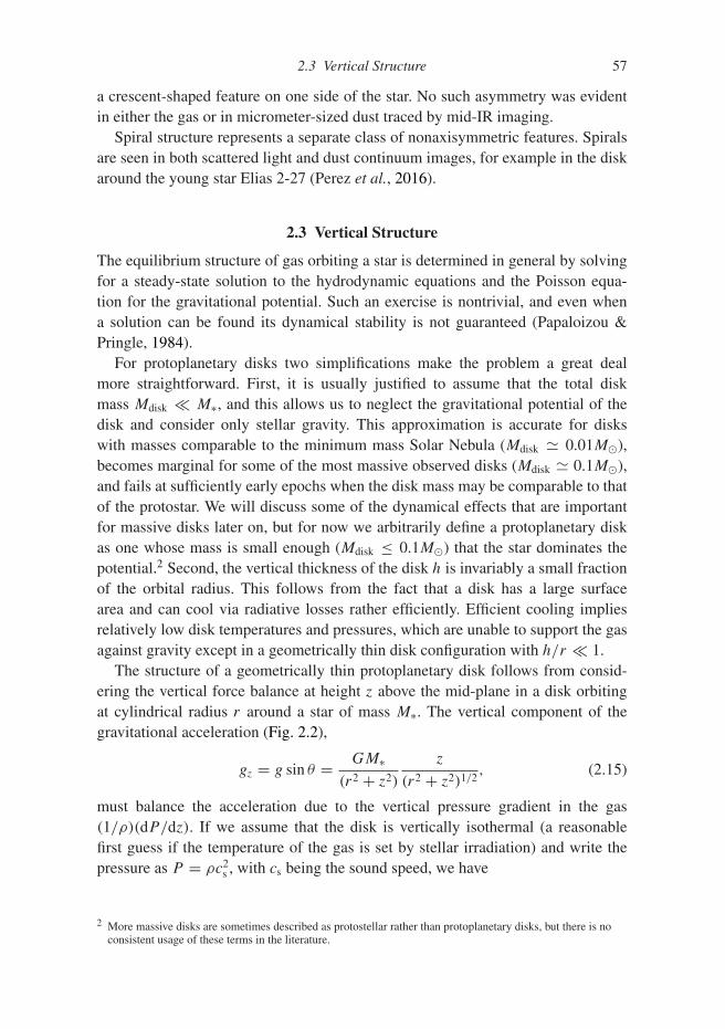
2.3 Vertical Structure 57
a crescent-shaped feature on one side of the star. No such asymmetry was evidentin either the gas or in micrometer-sized dust traced by mid-IR imaging.
Spiral structure represents a separate class of nonaxisymmetric features. Spiralsare seen in both scattered light and dust continuum images, for example in the diskaround the young star Elias 2-27 (Perez et al., 2016).
2.3 Vertical Structure
The equilibrium structure of gas orbiting a star is determined in general by solvingfor a steady-state solution to the hydrodynamic equations and the Poisson equa-tion for the gravitational potential. Such an exercise is nontrivial, and even whena solution can be found its dynamical stability is not guaranteed (Papaloizou &Pringle, 1984).
For protoplanetary disks two simplifications make the problem a great dealmore straightforward. First, it is usually justified to assume that the total diskmass Mdisk M∗, and this allows us to neglect the gravitational potential of thedisk and consider only stellar gravity. This approximation is accurate for diskswith masses comparable to the minimum mass Solar Nebula (Mdisk � 0.01M�),becomes marginal for some of the most massive observed disks (Mdisk � 0.1M�),and fails at sufficiently early epochs when the disk mass may be comparable to thatof the protostar. We will discuss some of the dynamical effects that are importantfor massive disks later on, but for now we arbitrarily define a protoplanetary diskas one whose mass is small enough (Mdisk ≤ 0.1M�) that the star dominates thepotential.2 Second, the vertical thickness of the disk h is invariably a small fractionof the orbital radius. This follows from the fact that a disk has a large surfacearea and can cool via radiative losses rather efficiently. Efficient cooling impliesrelatively low disk temperatures and pressures, which are unable to support the gasagainst gravity except in a geometrically thin disk configuration with h/r 1.
The structure of a geometrically thin protoplanetary disk follows from consid-ering the vertical force balance at height z above the mid-plane in a disk orbitingat cylindrical radius r around a star of mass M∗. The vertical component of thegravitational acceleration (Fig. 2.2),
gz = g sin θ = GM∗(r2 + z2)
z
(r2 + z2)1/2, (2.15)
must balance the acceleration due to the vertical pressure gradient in the gas(1/ρ)(dP/dz). If we assume that the disk is vertically isothermal (a reasonablefirst guess if the temperature of the gas is set by stellar irradiation) and write thepressure as P = ρc2
s , with cs being the sound speed, we have
2 More massive disks are sometimes described as protostellar rather than protoplanetary disks, but there is noconsistent usage of these terms in the literature.

58 Protoplanetary Disk Structure
r
zg
gz
q
Figure 2.2 The vertical structure of geometrically thin disks is set by a balancebetween the vertical component of the star’s gravity gz and a pressure gradient.
c2s
dρ
dz= − GM∗z
(r2 + z2)3/2ρ. (2.16)
The solution is
ρ = C exp
[GM∗
c2s (r
2 + z2)1/2
], (2.17)
where the constant of integration C is set by the mid-plane density. This expressionis rarely used. Rather, we note that for a thin disk z r and gz � �2z, where� =
√GM∗/r3 is the Keplerian angular velocity. In this limit the vertical density
profile has the simple form
ρ = ρ0e−z2/2h2, (2.18)
where the mid-plane density ρ0 can be written in terms of the full-plane surfacedensity � as
ρ0 = 1√2π
�
h, (2.19)
and h, the vertical disk scale-height, is given by
h ≡ cs
�. (2.20)
Note that this means that the geometric thickness of the disk h/r = M−1, wherethe Mach number of the flow M = vK/cs.
The assumptions that went into this calculation are generally self-consistent.Detailed disk models computed by Bell et al. (1997) show that for a disk accretingat a low rate onto a solar mass star the mid-plane temperature at 1 AU is aroundT � 100 K. The corresponding isothermal sound speed is
c2s = kBT
μmp, (2.21)
where kB is the Boltzmann constant and μ is the mean molecular weight in unitsof the proton mass mp. Taking μ = 2.3 for a fully molecular gas of cosmic com-position we have that cs ≈ 0.6 km s−1 and (at 1 AU around a solar mass star)h/r ≈ 0.02. The condition that the disk is geometrically thin is adequately satisfied.We should also verify that the vertical structure is not modified by the gravitational

2.4 Radial Force Balance 59
force from the disk itself. Representing the disk as a thin infinite sheet of mass withsurface density �, a straightforward application of Gauss’ theorem shows that theacceleration outside the sheet is constant with distance,
gz,disk = 2πG�. (2.22)
Equating this disk contribution to the acceleration due to the vertical componentof stellar gravity at z = h, the condition that the self-gravity of the disk can beneglected when computing the vertical structure becomes
� <M∗h2πr3
. (2.23)
For the minimum mass Solar Nebula at 1 AU this condition is satisfied by morethan an order of magnitude. More generally, if we write the enclosed disk mass asMdisk(r) ∼ πr2�, self-gravity is ignorable provided that
Mdisk
M∗<
1
2
(h
r
). (2.24)
At large radii h/r ∼ 0.1, so for a massive disk with Mdisk/M∗ = 0.1 theneglect of disk self-gravity in the calculation of the vertical structure is notjustified. Such disks require additional consideration, however, since the conditionMdisk/M∗ ∼ h/r also describes the mass above which disk self-gravity results inthe disk becoming unstable to the development of nonaxisymmetric structure inthe form of spiral waves. We discuss this separate (and more important) effect ofself-gravity in Chapter 3.
The shape of the disk depends upon h(r)/r . If we parameterize the radial varia-tion of the sound speed via
cs ∝ r−β, (2.25)
then the aspect ratio varies as
h
r∝ r−β+1/2. (2.26)
The disk will flare – i.e. h/r will increase with radius giving the disk a bowl-likeshape – if β < 1/2. This requires a temperature profile T (r) ∝ r−1 or shallower.In an unwarped flaring disk the star is visible from all points on the surface of thedisk.
2.4 Radial Force Balance
The density profile of the disk in the radial direction cannot be derived withouteither considering the nature of angular momentum transport, or by appealing toobservational constraints (such as the minimum mass Solar Nebula). The orbital
60 Protoplanetary Disk Structure
velocity of disk gas, however, can be determined given a surface density and tem-perature profile. We start from the momentum equation for an unmagnetized andinviscid fluid,
∂v∂t
+ (v · ∇)v = − 1
ρ∇P − ∇�, (2.27)
where v is the velocity, ρ the density, P the pressure, and � the gravitationalpotential. Specializing to a stationary axisymmetric flow in which the potential isdominated by that of the star, the radial component of the momentum equationimplies that the orbital velocity of the gas vφ,gas is given by
v2φ,gas
r= GM∗
r2+ 1
ρ
dP
dr. (2.28)
Since the pressure near the disk mid-plane normally decreases outward, the secondterm on the right-hand-side is negative and the azimuthal velocity of the gas isslightly less than the Keplerian velocity (Eq. 1.25) of a point mass particle orbitingat the same radius. To quantify the difference we write the variation of the mid-plane pressure as a power-law near some fiducial radius r0,
P = P0
(r
r0
)−n
, (2.29)
where P0 = ρ0c2s . Substituting we find that
vφ,gas = vK
(1 − n
c2s
v2K
)1/2
. (2.30)
Recalling the definition of the vertical scale-height (Eq. 2.20) we note that thedeviation from Keplerian velocity is O(h/r)2, and hence small for geometricallythin disks. For example, if the disk has a constant value of h(r)/r = 0.05 and asurface density profile � ∝ r−1 we obtain n = 3 and
vφ,gas � 0.996vK. (2.31)
When considering the motion of the gas alone this difference is utterly negligibleand we can safely assume the gas moves at the Keplerian velocity. The slightlylower gas velocity is however important for the evolution of solid bodies within thedisk, since it results in aerodynamic drag and resultant orbital decay.
2.5 Radial Temperature Profile of Passive Disks
The time scale for the disk to attain thermal equilibrium is generally much less thanthe time scale for evolution of either the disk or the star. The temperature profile ofthe disk is then set by the balance between cooling and heating, for which there aretwo main sources:

2.5 Radial Temperature Profile of Passive Disks 61
• Intercepted stellar radiation, which is absorbed (usually by dust) and subsequentlyreradiated at longer wavelengths. Disks for which this is the main heating processare described as passive disks.
• Dissipation of gravitational potential energy, as matter in the disk spirals in towardthe star.
The heating per unit area from both of these sources drops off with increasingdistance from the star. If the disk extends out to large enough radii, heating dueto the ambient radiation field provided by nearby stars can become significant andprevent the disk temperature from dropping below some floor level. For normal starforming environments this floor temperature might be 10–30 K.
The relative importance of accretional heating versus stellar irradiation dependsupon the accretion rate and the amount of intercepted stellar radiation. Globally,inspiralling matter will radiate an amount of energy per unit mass that is approx-imately given by the gravitational potential at the stellar surface, GM∗/R∗, whilethe disk will intercept a fraction f < 1 of the stellar radiation. Taking f = 1/4 (thecorrect result for a razor-thin disk that extends all the way to the stellar surface)the accretion rate M above which accretional heating dominates can be crudelyestimated as
GM∗MR∗
= 1
4L∗. (2.32)
For a young solar mass star with a luminosity L∗ = L� = 3.9 × 1033 erg s−1 and aradius R∗ = 2R�,
M ≈ 2 × 10⁻⁸ M� yr−1. (2.33)
Measured accretion rates for classical T Tauri stars range from an order of magni-tude above this critical rate to two orders of magnitude below, so it is oversimpli-fying to treat protoplanetary disks as being either always passive or always active.Rather, the thermal structure of disks at early epochs (when accretion is strongest)is likely dominated by internal heating due to the accretion, whereas at later timesreprocessing of stellar radiation dominates. At a single epoch, due to the flaringeffect discussed below, accretion heating is relatively more significant close tothe star.
2.5.1 Razor-Thin Disks
The temperature profile and spectral energy distribution of a passive protoplanetarydisk are determined by the shape of the disk (whether it is flat, flared, or warped)and by the mechanism by which the absorbed stellar radiation is re-emitted. Webegin by considering the simplest model: a flat razor-thin disk in the equatorial

62 Protoplanetary Disk Structure
qr
R*
Figure 2.3 Geometry for calculation of the radial temperature profile of a razor-thin protoplanetary disk. The flux impinging on the surface of the disk at distancer from the star is computed by integrating over the visible stellar surface.
plane that absorbs all incident stellar radiation and re-emits it locally as a singletemperature blackbody. The back-warming of the star by the disk is neglected.
We consider a surface in the plane of the disk at distance r from a star of radiusR∗. The star is assumed to be a sphere of constant brightness I∗. Setting up sphericalpolar coordinates such that the axis of the coordinate system points to the center ofthe star, as shown in Fig. 2.3, the stellar flux passing through this surface is
F =∫
I∗ sin θ cos φd�, (2.34)
where d� represents the element of solid angle. We count the flux coming from thetop half of the star only (and to be consistent equate that to radiation from only thetop surface of the disk), so the limits on the integral are
−π/2 < φ ≤ π/2,
0 < θ < sin−1
(R∗r
).
(2.35)
Substituting d� = sin θdθdφ, the integral for the flux is
F = I∗∫ π/2
−π/2cos φdφ
∫ sin−1(R∗/r)
0sin2 θdθ, (2.36)
which evaluates to
F = I∗
⎡⎣sin−1
(R∗r
)−
(R∗r
)√1 −
(R∗r
)2⎤⎦ . (2.37)
For a star with effective temperature T∗, the brightness I∗ = (1/π)σT 4∗ , with σ the
Stefan–Boltzmann constant (e.g. Rybicki & Lightman, 1979). Equating F to theone-sided disk emission σT 4
disk we obtain a radial temperature profile
(Tdisk
T∗
)4
= 1
π
⎡⎣sin−1
(R∗r
)−
(R∗r
)√1 −
(R∗r
)2⎤⎦ . (2.38)

2.5 Radial Temperature Profile of Passive Disks 63
Integrating over radii, we obtain the total disk luminosity,
Ldisk = 2 ×∫ ∞
R∗2πrσT 4
diskdr
= 1
4L∗. (2.39)
We conclude that a flat passive disk extending all the way to the stellar equator inter-cepts a quarter of the stellar flux. The ratio of the observed bolometric luminosityof such a disk to the stellar luminosity will vary with viewing angle, but clearly aflat passive disk is predicted to be less luminous than the star.
The form of the temperature profile given by Eq. (2.38) is not very transparent.Expanding the right-hand-side in a Taylor series in the limit that (R∗/r) 1 (i.e.far from the stellar surface), we obtain
Tdisk ∝ r−3/4, (2.40)
as the limiting temperature profile of a thin, flat, passive disk. For fixed molecularweight μ this in turn implies a sound speed profile
cs ∝ r−3/8. (2.41)
Assuming vertical isothermality, the aspect ratio given by Eq. (2.26) is
h
r∝ r1/8, (2.42)
and we predict that the disk ought to flare modestly to larger radii. If the disk doesflare then the outer regions intercept a larger fraction of stellar photons, leadingto a higher temperature. As a consequence, a temperature profile Tdisk ∝ r−3/4 isprobably the steepest profile we would expect to obtain for a passive disk.
2.5.2 Flared Disks
The next step in sophistication is to consider a flared disk. If at cylindrical distancer from the star the disk absorbs stellar radiation at a height hp above the mid-plane,the disk is described as flared if the ratio hp/r is an increasing function of radius.Features of flared disks are, first, that all points on the surface of the disk have aclear line of sight to the star and, second, that as seen from the star the disk subtendsa greater solid angle than a razor-thin disk. Flared disks absorb a greater fractionof the stellar radiation than flat disks, and thus produce stronger IR excesses. Thetemperature profile is also modified and this changes the shape of the resulting SED.
The temperature profile of a flared disk can be computed in the same way asfor a razor-thin disk, namely by evaluating the flux (Eq. 2.34) by integrating overthe part of the stellar surface visible from the disk surface at radius r . The exactcalculation can be found in the appendix to Kenyon and Hartmann (1987), and

64 Protoplanetary Disk Structure
r
hp
Angle α between radiation andtangent to disk surface
Figure 2.4 Geometry for calculation of the radial temperature profile of a flaredprotoplanetary disk. At distance r � R∗, radiation from the star is absorbed bythe disk at height hp above the mid-plane. The angle between the tangent to thedisk surface and the radiation is α.
while it is conceptually simple some messy geometry is required. Here we adoptan approximate treatment valid for r � R∗, and consider the star to be a pointsource of radiation. At cylindrical distance r , stellar radiation is absorbed by thedisk at height hp above the mid-plane. Note that hp is not the same as the disk scale-height h, since the absorption of stellar radiation depends not just on the density butalso on the opacity of the disk material to stellar photons (the height of the disk’sphotosphere – i.e. the surface at which the optical depth to the disk’s own thermalradiation is τ = 2/3 – is yet a third different height). From consideration of thegeometry in Fig. 2.4 the angle between the incident radiation and the local disksurface is given by3
α = dhp
dr− hp
r. (2.43)
The rate of heating per unit disk area at distance r is
Q+ = 2α
(L∗
4πr2
), (2.44)
where the factor of two comes from the fact that the disk has two sides and we haveassumed that all of the stellar surface is visible from the surface of the disk (i.e. thatthe optically thick disk does not extend all the way to the stellar surface). Equatingthe heating rate to the rate of cooling by blackbody radiation,
Q− = 2σT 4disk, (2.45)
the temperature profile becomes
Tdisk =(
L∗4πσ
)1/4
α1/4r−1/2. (2.46)
Since L∗ = 4πR2∗σT 4
∗ an equivalent expression is
Tdisk
T∗=
(R∗r
)1/2
α1/4. (2.47)
3 A more accurate approximation including a correction for the finite size of the star isα � 0.4R∗/r + rd(hp/r)/dr .

2.5 Radial Temperature Profile of Passive Disks 65
The interior of an irradiated protoplanetary disk can reasonably be assumed tobe isothermal, so this equation specifies the central sound speed and hence thevertical scale-height h via Eq. (2.20). If we additionally specify a relation betweenh and hp – for example by assuming that hp ∝ h, which may be plausible if thedisk is very optically thick – then Eqs. (2.20), (2.21), (2.43), and (2.47) form aclosed system of equations whose solution determines α. At large radii, Kenyonand Hartmann (1987) find that the surface temperature approaches
Tdisk(r) ∝ r−1/2, (2.48)
which is as expected substantially flatter than the Tdisk ∝ r−3/4 profile of a flat disk(Eq. 2.40).
2.5.3 Radiative Equilibrium Disks
Thus far we have assumed that the stellar radiation intercepted by the disk is rera-diated as a single temperature blackbody. Additional complexity arises for realdisks because the dominant opacity is provided by dust, which absorbs relativelyshort wavelength starlight (at around 1μm) more efficiently than it emits longerwavelength thermal radiation. Figure 2.5 depicts the absorption and reradiationof stellar radiation for an optically thick disk in which dust is mixed evenly withthe gas in the vertical direction. Short wavelength stellar radiation is absorbed bydust within a relatively thin surface layer for which the optical depth to grazingstarlight τ <∼ 1. The layer is optically thin (τ 1) to the longer wavelength thermal
Disk interior
Figure 2.5 The physics underlying radiative equilibrium models for protoplan-etary disks. Stellar radiation is absorbed in a thin surface layer by dust, whichreradiates in the infrared both upward into space and downward where it isabsorbed once more and acts to heat the disk interior. The local emission fromthe disk is a superposition of radiation from the hot surface layer and the coolerinterior.

66 Protoplanetary Disk Structure
radiation emitted by the hot dust. Approximately half of the incoming stellar fluxis then reradiated directly to space, while the downward directed half is absorbedby and heats the interior of the disk. The local emission from the disk is then asuperposition of a cool blackbody component from the disk interior with a warmerdilute blackbody generated by the surface layer.
The temperature of the dust in the surface layer can be calculated given knowl-edge of the radiative properties of the dust. We define the emissivity ε as theratio of the efficiency with which the dust emits or absorbs radiation relative toa blackbody surface (by definition a perfect absorber and emitter with ε = 1). Dustis generally a good absorber of radiation at wavelengths that are small compared tothe particle size, with the emissivity dropping at longer wavelengths. For sphericaldust particles of radius s we have, approximately,
ε = 1, λ ≤ 2πs,
ε =(
λ
2πs
)−1
, λ > 2πs.(2.49)
This is equivalent to assuming that the wavelength dependence of the mono-chromatic opacity κν ∝ λ−1. If a dust particle at radius r is exposed to a stellarflux F∗ = L∗/(4πr2), its equilibrium temperature Tdust is determined by balancingheating at a rate πs2ε∗F∗, where ε∗ is the weighted emissivity for absorption of thestellar radiation spectrum, with cooling at a rate 4πs2σT 4
dustεdust, where εdust is theweighted emissivity for the dust particle’s thermal emission. Equating,
Tdust
T∗=
(ε∗
εdust
)1/4 (R∗2r
)1/2
. (2.50)
For particles that are small enough such that ε < 1 for both absorption of stellarradiation and emission of thermal radiation, we can estimate the ratio ε∗/εdust byevaluating the emissivity at the wavelength where thermal radiation peaks. We thenhave that ε ∝ λ−1 ∝ T , so that ε∗/εdust = T∗/Tdust. Substituting in Eq. (2.50),
Tdust
T∗=
(R∗2r
)2/5
. (2.51)
Since the mismatch between the emissivity for absorption and emission becomesmore severe at larger radii, the temperature of dust exposed to stellar radiation at thedisk surface drops even more slowly with increasing distance than the temperatureof a single temperature flared disk. Inserting fiducial values for the stellar radiusR∗ = 2R� and stellar effective temperature T∗ = 4000 K we find that
Tdust = 470( r
1 AU
)−2/5K. (2.52)
This scaling was derived by Chiang and Goldreich (1997).

2.5 Radial Temperature Profile of Passive Disks 67
This analysis assumes that the dust particles can be considered in isolation,whereas in reality they are embedded within gas whose temperature will not ingeneral be equal to the dust temperature given by Eq. (2.50). If Tgas < Tdust, colli-sions between molecules and the dust particles will result in nonradiative coolingof the dust. If this cooling process is efficient enough it will invalidate the radiativeequilibrium that was assumed in deriving Eq. (2.50).
To evaluate the conditions for which it is reasonable to assume that the dust andgas are thermally decoupled, we note that collisions between molecules and dustparticles occur at a rate (per unit area of dust) ngasvth, where ngas is the numberdensity of molecules, and vth, the thermal velocity of the molecules, is given by
vth =(
8kBTgas
πμmH
)1/2
, (2.53)
where μmH is the mean particle mass. Each collision carries away of the order ofkBTdust worth of energy. Collisions will be ignorable for thermal equilibrium of dustparticles if
kTdustngasvth < εdustσT 4dust. (2.54)
Evaluating the thermal velocity of the gas assuming that its temperature is compa-rable to that of the dust, we find that collisions can be neglected provided that
ngas <(π
8
)1/2 (μmH)1/2
k3/2B
εdustσT5/2
dust . (2.55)
The two-temperature disk model of Fig. 2.5 will therefore persist provided that thegas density in the region where dust is marginally optically thick to stellar radiationis low enough. To give a specific example, we can estimate whether a model inwhich the gas and dust temperatures are unequal is self-consistent at 1 AU, wherewe would predict that Tdust = 470 K. For dust particles whose size is such thatεdust � 0.1 the above expression suggests that collisions with hydrogen moleculesare ignorable for gas densities ngas
<∼ 2 × 1013 cm−3. Taking a minimum massSolar Nebula surface density at 1 AU of 1.7 × 10³ g cm−2 with h/r = 0.05, themid-plane hydrogen number density is a few ×1014 cm−3. The dust and the gaswill therefore be thermally coupled if the dust has settled to the mid-plane andabsorbs stellar radiation there. Conversely, ngas will be below the threshold forthermal coupling if the dust is well mixed with the gas and absorption occurs ata height z >∼ 2.5h. Evidently the extent of dust–gas energy exchange at 1 AU israther subtle, and strictly it cannot be considered in isolation from questions of dustsettling and agglomeration. At larger radii, where the surface density is smaller andthe scale-height larger, the effect of collisions on the thermal state of irradiated dustcan more safely be neglected.
For studies of disk chemistry, and for modeling of molecular line observations,the gas temperature is of more importance than that of the dust. If the density is

68 Protoplanetary Disk Structure
high enough, the thermal accommodation process discussed above will establish acommon temperature for both, and there is no need to explicitly consider the ther-mal physics of the gas. At lower optical depth, however, Tgas �= Tdust. In particular,gas that is exposed to stellar UV photons is strongly heated by the photoelectriceffect. The work function of graphite grains (the minimum energy required to freean electron from them) is around 5 eV, so 10 eV far ultraviolet (FUV) photons caneject electrons from uncharged grains with 5 eV of kinetic energy that is ultimatelythermalized and acts to heat the gas. The ejection probability is of the order of 0.1,so the overall efficiency (the fraction of incident FUV energy that goes into heatingthe gas) can be rather high, around 5%.
Thermal models of gaseous protoplanetary disks include photoelectric heating,cooling via line radiation, and energy exchange with dust, among other processes.The qualitative picture of gas disk structure that emerges includes three layers.
• A cool mid-plane region, where Tgas ≈ Tdust and dust cooling is dominant.
• A warm surface layer in which both dust and gas have temperatures that exceedthe mid-plane value. The gas in the warm layer can be substantially hotter thanthe dust (T ∼ 103 K at 1 AU), and cools both by dust–gas collisions and by COrotational–vibrational transitions.
• A hot, low density atmosphere, where Lyα radiation and other atomic lines coolthe gas.
2.5.4 The Chiang–Goldreich Model
Although computation of disk models that include all of the aforementioned physicsgenerally requires numerical techniques, useful analytic approximations are avail-able. The most widely used is that developed by Chiang and Goldreich (1997). Theyconsidered a disk surrounding a 0.5 M� star with radius R∗ = 2.5 R� and effectivetemperature T∗ = 4000 K. The disk has a surface density profile �(r) ∝ r−3/2, asurface density at 1 AU of 103 g cm−2, and a dust to gas ratio of 10−2. The resultingtemperature of dust at the surface of the disk is
Tdust = 550( r
1 AU
)−2/5K. (2.56)
The temperature of the disk interior Ti and the height of the visible photosphere hp
are approximated by piecewise polynomials. At 0.4 AU < r < 84 AU,
Ti = 150( r
1 AU
)−3/7K,
hp
r= 0.17
( r
1 AU
)2/7.
(2.57)
2.5 Radial Temperature Profile of Passive Disks 69
At 84 AU < r < 209 AU,
Ti = 21 K,
hp
r= 0.064
( r
1 AU
)1/2.
(2.58)
At 209 AU < r < 270 AU,
Ti = 200( r
1 AU
)−19/45K,
hp
r= 0.20
( r
1 AU
)13/45.
(2.59)
These expressions, which can be generalized without difficulty to other stellar ordisk properties, are quite useful in practice for giving an idea of the physical con-ditions within weakly accreting protoplanetary disks. Their main limitation arisesfrom the fact that in ignoring heating due to accretion they tend to underestimate thetemperature at the disk mid-plane. This deficiency can be remedied (e.g. Garaud &Lin, 2007), but there remains considerable uncertainty in all disk models due to theuncertain distribution (both radially and vertically) of dust and its evolution overtime.
2.5.5 Spectral Energy Distributions
The spectral energy distribution of the disk can be computed by summing up thelocal disk emission at each radius, weighted by the area. The simplest case is whereeach annulus in the disk radiates as a blackbody at the local temperature Tdisk(r). Ifthe disk extends from rin to rout the disk spectrum is
Fλ ∝∫ rout
rin
2πrBλ[Tdisk(r)]dr, (2.60)
where Bλ is the Planck function,
Bλ(T ) = 2hc2
λ5
1
exp[hc/λkBT ] − 1. (2.61)
The behavior of the spectrum implied by Eq. (2.60) is easy to derive. At longwavelengths λ � hc/kBTdisk(rout) we recover the Rayleigh–Jeans form
λFλ ∝ λ−3, (2.62)
while at short wavelengths λ hc/kBTdisk(rin) there is an exponential cut-off thatmatches that of the hottest annulus in the disk,
λFλ ∝ λ−4 exp
[ −hc
λkBTdisk(rin)
]. (2.63)

70 Protoplanetary Disk Structure
For intermediate wavelengths,
hc
kBTdisk(rin) λ hc
kBTdisk(rout), (2.64)
the form of the spectrum depends upon the radial profile of the disk temperaturedistribution. For the razor-thin disk model with Tdisk(r) ∝ r−3/4 we substitute
x ≡ hc
λkBTdisk(rin)
(r
rin
)3/4
, (2.65)
into Eq. (2.60). We then have, approximately,
Fλ ∝ λ−7/3∫ ∞
0
x5/3dx
ex − 1∝ λ−7/3, (2.66)
and so
λFλ ∝ λ−4/3. (2.67)
The overall spectrum, shown schematically in Fig. 2.6, is that of a “stretched”blackbody (Lynden-Bell & Pringle, 1974). This simple spectrum is too steep inthe infrared to account for the observed properties of Class I and many Class IIsources. The more realistic flared disk models, or those that incorporate a warmsurface layer, yield flatter spectral energy distributions in the infrared which areable to reproduce the features of many YSO SEDs.
( )
Figure 2.6 The spectral energy distributions (λFλ, plotted in arbitrary units onthe vertical axis) of disks radiating as multicolor blackbodies with temperatureprofiles Tdisk(r) ∝ r−1/2 (upper curve) and Tdisk(r) ∝ r−3/4 (lower curve). Forthese toy models the disk was assumed to have a temperature of 1000 K at theinner edge at 0.1 AU, and to extend out to 30 AU.

2.6 Opacity 71
2.6 Opacity
Dust is the dominant opacity source within protoplanetary disks everywhere exceptin the very innermost regions, where the temperature is high enough (T � 1500 K)for dust particles to be destroyed leaving only molecular opacity. For an individualdust particle the cross-section to radiation of a given wavelength will depend uponthe particle size, structure (for example the particle may have a spherical or morecomplex geometry), and composition. At a particular location within the disk, thetotal opacity due to dust will depend primarily upon the temperature and chemicalcomposition of the disk (which determine which types of dust or ice are present) andthe size distribution of the particles, which may change as coagulation proceeds.To a lesser extent, the gas density also influences the opacity by modifying thetemperatures at which different species of dust particle are predicted to evaporate.Given a model for each of the above effects, it is possible to compute the frequency-dependent opacity κν of the gas and dust within the disk as a function of disktemperature and density.
Within the inner disk (where “inner” encompasses most of the radii of greatestinterest for planet formation) it is typically true that the mean-free path of ther-mal radiation from the disk interior is small compared to the disk scale-height. Inthis regime the radiation field is approximately isotropic and blackbody and theflux is proportional to the gradient of the energy density of the radiation Frad =−c∇(aT 4)/(3κRρ). The relevant opacity that enters into the equation for the fluxis the Rosseland mean,
1
κR=
∫ ∞0 (1/κν)(∂Bν/∂T )dν∫ ∞
0 (∂Bν/∂T )dν, (2.68)
where Bν is the Planck function.Figure 2.7 shows the temperature dependence of the Rosseland mean opacity
for dusty gas of density 10−9 g cm−3, as calculated by Semenov et al. (2003). Theelemental abundances represent best estimates of the solar values. The assumed sizedistribution of particles follows that proposed by Pollack et al. (1985):
n(s) = 1, s < 0.005 μm,
n(s) =(
s
0.005 μm
)−3.5
, 0.005 μm ≤ s < 1μm,
n(s) = 4 × 10⁴
(s
0.005 μm
)−5.5
, 1 μm ≤ s < 5μm,
n(s) = 0, s ≥ 5 μm.
(2.69)
This distribution is itself a modified version of the Mathis et al. (1977) distribu-tion which was derived based on observations of the wavelength dependence ofstellar extinction. The specific model plotted assumes that the dust is composed ofhomogeneous spherical particles.
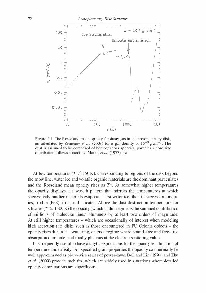
72 Protoplanetary Disk Structure
( )
()
IS
Figure 2.7 The Rosseland mean opacity for dusty gas in the protoplanetary disk,as calculated by Semenov et al. (2003) for a gas density of 10−9 g cm−3. Thedust is assumed to be composed of homogeneous spherical particles whose sizedistribution follows a modified Mathis et al. (1977) law.
At low temperatures (T <∼ 150 K), corresponding to regions of the disk beyondthe snow line, water ice and volatile organic materials are the dominant particulatesand the Rosseland mean opacity rises as T 2. At somewhat higher temperaturesthe opacity displays a sawtooth pattern that mirrors the temperatures at whichsuccessively hardier materials evaporate: first water ice, then in succession organ-ics, troilite (FeS), iron, and silicates. Above the dust destruction temperature forsilicates (T � 1500 K) the opacity (which in this regime is the summed contributionof millions of molecular lines) plummets by at least two orders of magnitude.At still higher temperatures – which are occasionally of interest when modelinghigh accretion rate disks such as those encountered in FU Orionis objects – theopacity rises due to H− scattering, enters a regime where bound–free and free–freeabsorption dominate, and finally plateaus at the electron scattering value.
It is frequently useful to have analytic expressions for the opacity as a function oftemperature and density. For specified grain properties the opacity can normally bewell approximated as piece-wise series of power-laws. Bell and Lin (1994) and Zhuet al. (2009) provide such fits, which are widely used in situations where detailedopacity computations are superfluous.

2.7 The Condensation Sequence 73
2.7 The Condensation Sequence
Since stars and their disks form from the collapse of the same material it is rea-sonable to assume that the elemental abundances in the disk (i.e. the ratio of theabundance of each element to the abundance of hydrogen) are very similar to thosein the star. For the Solar System, the measured solar photospheric abundances,supplemented by abundances derived from a small number of primitive chondriticmeteorites, provide a proxy for the primordial Solar Nebula composition. Even oncethe raw abundances are known, however, there remains the task of determining thechemical composition of the disk – i.e. how the elements are distributed among thepossible chemical compounds and states – as a function of radius and time. This isnot an easy task. Oxygen, for example, may be present in many forms, includingcarbon monoxide (CO), water (H2O) in the form of vapor or ice, oxides such asFe3O4, and silicates such as Mg2SiO4. The distribution of oxygen between these(and many other) forms will affect the opacity in the disk, the total surface densityof solid materials, and the composition of larger bodies that form at a given radius.
The most general formulation of the problem of determining the composition ofthe disk is as an initial value problem. If the initial composition of the disk withradius is known, a chemical network describing the rates of possible reactions canbe integrated forward in time to determine the composition at subsequent epochs.This approach allows for the disk’s chemical composition to be out of equilibrium(for example in the outer disk, where the low temperatures mean that the rates ofenergetically favorable reactions can be very low), and can be readily extended toaccommodate radial flow as the disk evolves.
In practice, solving for the evolution of a disk coupled to a fully consistenttreatment of the chemistry is challenging. It is therefore useful to pose a simplerquestion: for a given temperature and pressure what composition is the most ther-modynamically stable? Conceptually, we can imagine starting with a high temper-ature gas in which all of the elements are in the vapor phase and cooling it veryslowly so that the elements successively condense out into various solid phases.Provided that the cooling is slow enough all reactions will have sufficient time toreach equilibrium, and the resulting condensation sequence will depend only onthe abundances, the temperature, and the pressure. Under conditions of constanttemperature and pressure, the thermodynamically preferred state is the one thatminimizes the Gibbs free energy,
G ≡ H − T S, (2.70)
where H is the enthalpy and S the entropy. If the chemical system comprises anumber of homogeneous (or ideal) phases, i = 1,2, . . . ,
G = � (μifi) , (2.71)
where fi is the fraction in phase i with chemical potential μi . The compositioncan then be determined by finding the fi that minimize G, subject to the constraint
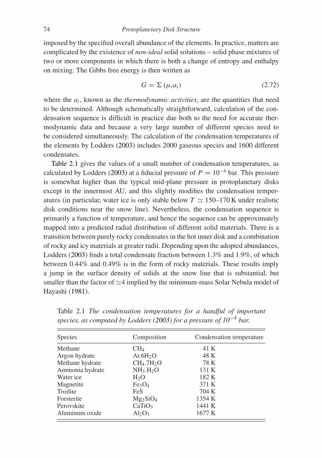
74 Protoplanetary Disk Structure
imposed by the specified overall abundance of the elements. In practice, matters arecomplicated by the existence of non-ideal solid solutions – solid phase mixtures oftwo or more components in which there is both a change of entropy and enthalpyon mixing. The Gibbs free energy is then written as
G = � (μiai) (2.72)
where the ai , known as the thermodynamic activities, are the quantities that needto be determined. Although schematically straightforward, calculation of the con-densation sequence is difficult in practice due both to the need for accurate ther-modynamic data and because a very large number of different species need tobe considered simultaneously. The calculation of the condensation temperatures ofthe elements by Lodders (2003) includes 2000 gaseous species and 1600 differentcondensates.
Table 2.1 gives the values of a small number of condensation temperatures, ascalculated by Lodders (2003) at a fiducial pressure of P = 10−4 bar. This pressureis somewhat higher than the typical mid-plane pressure in protoplanetary disksexcept in the innermost AU, and this slightly modifies the condensation temper-atures (in particular, water ice is only stable below T � 150–170 K under realisticdisk conditions near the snow line). Nevertheless, the condensation sequence isprimarily a function of temperature, and hence the sequence can be approximatelymapped into a predicted radial distribution of different solid materials. There is atransition between purely rocky condensates in the hot inner disk and a combinationof rocky and icy materials at greater radii. Depending upon the adopted abundances,Lodders (2003) finds a total condensate fraction between 1.3% and 1.9%, of whichbetween 0.44% and 0.49% is in the form of rocky materials. These results implya jump in the surface density of solids at the snow line that is substantial, butsmaller than the factor of �4 implied by the minimum-mass Solar Nebula model ofHayashi (1981).
Table 2.1 The condensation temperatures for a handful of importantspecies, as computed by Lodders (2003) for a pressure of 10−4 bar.
Species Composition Condensation temperature
Methane CH4 41 KArgon hydrate Ar.6H2O 48 KMethane hydrate CH4.7H2O 78 KAmmonia hydrate NH3.H2O 131 KWater ice H2O 182 KMagnetite Fe3O4 371 KTroilite FeS 704 KForsterite Mg2SiO4 1354 KPerovskite CaTiO3 1441 KAluminum oxide Al2O3 1677 K
2.8 Ionization State of Protoplanetary Disks 75
2.8 Ionization State of Protoplanetary Disks
The interior temperatures of typical protoplanetary disks range from a few thousandK in the immediate vicinity of the star to just tens of K in the outer regions. Thesetemperatures are not high enough to ionize the gas fully. As a rule of thumb, anelement with an ionization potential χ is ionized once the temperature exceeds
T ∼ χ
10kB. (2.73)
The ionization temperature for hydrogen is about 104 K and even potassium – oneof the most easily ionized species with χ = 4.34 eV – requires T >∼ 5000 Kbefore it becomes ionized. As a first and excellent approximation we can there-fore assume that protoplanetary disks are neutral. However, as we will see laterwhen we discuss disk evolution, even apparently negligible ionization fractionssuffice to couple magnetic fields dynamically to the gas, and this coupling in turnmay be a critical element that permits angular momentum transport and accretion.An accurate understanding of the ionization fraction of protoplanetary disks as afunction of radius and height above the mid-plane is thus important. This requiresbalancing ionization sources, which may be thermal or nonthermal (radioactivedecay of short-lived nuclides, stellar X-rays, or cosmic rays), against recombina-tions in the gas phase or on the surfaces of dust grains. In more complex models itmay be necessary to go beyond such equilibrium considerations and allow for thepossibility that (relatively) well-ionized gas may be mixed by turbulent processesinto neutral regions on a time scale shorter than the recombination time (Turneret al., 2007; Ilgner & Nelson, 2008).
2.8.1 Thermal Ionization
Thermal ionization of the alkali metals dominates the ionization balance in thevery innermost regions of the disk, usually well inside 1 AU. This regime canbe treated straightforwardly. In thermal equilibrium the ionization state of asingle species with ionization potential χ is described by the Saha equation (e.g.Rybicki & Lightman, 1979):
nionne
n= 2U ion
U
(2πmekBT
h2
)3/2
exp[−χ/kBT ]. (2.74)
In this equation, nion and n are the number densities of the ionized and neutralspecies, and ne (= nion) is the electron number density. The partition functions forthe ions and neutrals are U ion and U respectively. The electron mass is me. Theslightly modified temperature dependence (an extra factor of T 3/2) as compared tothe Boltzmann factor, which governs the occupancy of atomic energy levels, arisesbecause the ionized state is favored on entropy grounds over the neutral state.

76 Protoplanetary Disk Structure
( )
,
Figure 2.8 The Saha equation prediction for the ionization state of the disk dueto the thermal ionization of potassium (ionization potential χ = 4.34 eV). Thefractional abundance of potassium has been taken to be f = 10−7, and the totalnumber density of neutrals nn = 1015 cm−3.
In protoplanetary disks the first significant source of thermal ionization ariseswhen the temperature becomes high enough to start ionizing the alkali metals. Forpotassium, the ionization potential χ = 4.34 eV. We write the fractional abundanceof potassium relative to all other neutral species as f = nK/nn, and define theionization fraction x as
x ≡ ne
nn. (2.75)
While potassium remains weakly ionized, the Saha equation yields
x � 10−12
(f
10−7
)1/2 ( nn
1015 cm−3
)−1/2(
T
103 K
)3/4
× exp[−2.52 × 10⁴/T ]
1.14 × 10⁻¹¹, (2.76)
where the final numerical factor in the denominator is the value of the exponentat the fiducial temperature of 103 K. The predicted ionization fraction is shown asa function of temperature in Fig. 2.8. Ionization fractions that are large enough tobe interesting for studies of magnetic field coupling are attained at temperaturesof T ∼ 103 K, although the numbers are still extremely small – of the order ofx ∼ 10−12 for our assumed parameters.
2.8.2 Nonthermal Ionization
Outside the inner thermally ionized region, disk irradiation by stellar X-rays, cos-mic rays, and radioactive decay of short-lived nuclides can all be significant sources
2.8 Ionization State of Protoplanetary Disks 77
of nonthermal ionization. Although the basic physics of each of these mechanismsis reasonably well understood there is at least an order of magnitude uncertaintyin the absolute value of the resulting ionization rates. To calculate the ionizationfraction, which is the quantity of interest for most purposes, requires knowledge ofboth the ionization and recombination rates, and poor understanding of the latterintroduces large additional uncertainties.
T Tauri stars are extremely luminous X-ray sources as compared to main-sequence stars of the same mass. Many disk-bearing classical T Tauri starsare detected in X-ray surveys of star forming regions, often with a soft X-rayluminosity in the range of 1028.5–1030.5 erg s−1 (Feigelson & Montmerle, 1999;Feigelson et al., 2007). Flares are observed with substantially higher luminosities.The spectra in the X-ray band are complex and include both line and continuumemission, which can be represented as a superposition of optically thin thermalbremsstrahlung components. The hardest spectral components have TX ∼ few keV,which implies a tail of emission extending out to energies of 10 keV or more.Analysis of the X-ray properties supports an interpretation of the emission asoriginating in a magnetically powered corona that is a scaled-up version (both inpower and in the size of the X-ray emitting magnetic field loops) of the Sun’s.The existence of many other diagnostics of stellar magnetic activity, includingZeeman splitting of optical spectral lines and nonthermal radio emission, supportthis conclusion.
Some fraction of the stellar X-ray luminosity will be intercepted by the disk,either directly or following scattering in the disk atmosphere or in a stellar wind. Ifthe gas is depleted of heavy elements (i.e. grains have condensed) the photoioniza-tion cross-section can be fit with a power-law (Igea & Glassgold, 1999),
σ(E) = 8.5 × 10⁻²³
(E
keV
)−2.81
cm2. (2.77)
The steep power-law dependence of the cross-section with energy means that thepenetrating power of X-rays is strongly energy dependent. X-rays with E = 1 keVare absorbed by a column �� 1 g cm−2, while at 5 keV the stopping depthis a few g cm−2. The outermost skin of the disk will therefore be ionized by softX-rays, while the hard tail of the spectrum will penetrate further toward the interior.Expressions for computing the attenuation are given in Krolik and Kallman (1983)and in Fromang et al. (2002). For our purposes, it suffices to consider a rough fit tonumerical results published by Igea and Glassgold (1999). For an X-ray luminosityof LX = 2 × 1030 erg s−1 and a 5 keV thermal spectrum, Turner and Sano (2008) fitan ionization profile of the form
ζX = 2.6 × 10⁻¹⁵( r
1 AU
)−2exp[−��/�stop] s−1, (2.78)
where �� is the column density measured downward from the disk surface and�stop = 8 g cm−2 is an approximate stopping depth.
78 Protoplanetary Disk Structure
The high column density of gas in the inner regions of protoplanetary disksmeans that even the hardest stellar X-rays measured to date will be unable to pene-trate to the disk mid-plane. Interstellar cosmic rays have a spectrum that extends upto much higher energies, with correspondingly greater penetrating power. Adoptingthe fiducial value for the interstellar cosmic ray flux (Spitzer & Tomasko, 1968) theresulting ionization rate is
ζCR = 10−17 exp[−��/�stop] s−1, (2.79)
where in this case �stop = 102 g cm−2 (Umebayashi & Nakano, 1981). The maindifficulty in applying this expression to protoplanetary disks comes from the uncer-tain effect of stellar winds on the cosmic ray flux. The solar wind – which isprobably much less powerful than typical T Tauri winds – is able to modulate theflux of Galactic cosmic rays measured at the Earth, and it is quite conceivable thatT Tauri winds (from either the star or the disk) may be able to exclude the bulk of theinterstellar cosmic ray flux. Equation (2.79) is therefore realistically an upper limitto the ionization expected from cosmic rays, and the actual cosmic ray ionizationrate could be negligibly small.
Radioactive decay provides a final source of ionization. It takes about �ε =36 eV to produce an ion pair in molecular hydrogen, so a decay that yields anamount of energy E will create about E/�ε ions. If the nuclide under considerationhas a fractional abundance (relative to hydrogen) f and a decay constant λ,4 theionization rate is (Stepinski, 1992)
ζR = λf E
�ε. (2.80)
Abundant short-lived nuclides yield the highest ionization rates. Provided that it isoriginally present and has not yet had time to decay, 26Al is predicted to dominate.Note that 26Al has a very short half-life of 0.72 Myr (λ � 3 × 10⁻¹⁴ s−1), anenergy per decay of E = 3.16 MeV, and an estimated Solar System abundance off ∼ 10−10. With these parameters ζR � 2.6 × 10⁻¹⁹ s−1, though this value willdrop substantially over the disk lifetime due to the ongoing exponential decay. Therate may be further suppressed if the radioactive material is locked up within smallpebble-sized solid bodies, and may be zero if the disk in question was not pollutedwith material from a relatively recent supernova.
Figure 2.9 shows the ionization rate as a function of column density for thesimple models of X-ray, cosmic ray, and radioactive ionization discussed above.Despite the numerous uncertainties it is safe to conclude that X-ray ionizationwill dominate all other sources close to the disk surface, down to a column of10–100 g cm−2. Close to the mid-plane in the inner disk – where � > 103 g cm−2 –either cosmic rays or 26Al decays can potentially furnish a lower level of ionization.
4 Related to the half-life via t1/2 = ln 2/λ.
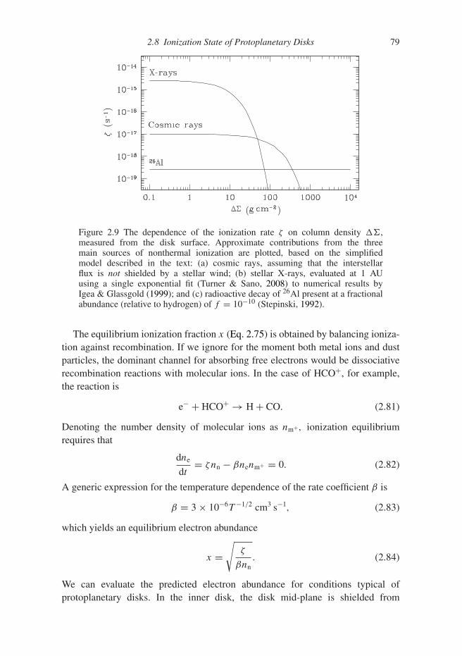
2.8 Ionization State of Protoplanetary Disks 79
( )
( )
Figure 2.9 The dependence of the ionization rate ζ on column density ��,measured from the disk surface. Approximate contributions from the threemain sources of nonthermal ionization are plotted, based on the simplifiedmodel described in the text: (a) cosmic rays, assuming that the interstellarflux is not shielded by a stellar wind; (b) stellar X-rays, evaluated at 1 AUusing a single exponential fit (Turner & Sano, 2008) to numerical results byIgea & Glassgold (1999); and (c) radioactive decay of 26Al present at a fractionalabundance (relative to hydrogen) of f = 10−10 (Stepinski, 1992).
The equilibrium ionization fraction x (Eq. 2.75) is obtained by balancing ioniza-tion against recombination. If we ignore for the moment both metal ions and dustparticles, the dominant channel for absorbing free electrons would be dissociativerecombination reactions with molecular ions. In the case of HCO+, for example,the reaction is
e− + HCO+ → H + CO. (2.81)
Denoting the number density of molecular ions as nm+, ionization equilibriumrequires that
dne
dt= ζnn − βnenm+ = 0. (2.82)
A generic expression for the temperature dependence of the rate coefficient β is
β = 3 × 10⁻⁶T −1/2 cm3 s−1, (2.83)
which yields an equilibrium electron abundance
x =√
ζ
βnn. (2.84)
We can evaluate the predicted electron abundance for conditions typical ofprotoplanetary disks. In the inner disk, the disk mid-plane is shielded from

80 Protoplanetary Disk Structure
cosmic rays and a representative ionization rate due to radioactive decay mightbe ζ ∼ 10−19 s−1. For nn = 1015 cm−3 and T = 300 K we obtain x � 2.4 × 10⁻¹⁴.For the same temperature close to the disk surface we may have nn = 1010 cm−3
and a substantially enhanced ionization rate due to stellar X-rays, ζX ∼ 10−15 s−1.These parameters yield x � 7.6 × 10⁻¹⁰. Although both values may appearnegligibly small, in fact the difference is sufficient to imply substantially differentcoupling between the gas and magnetic fields.
The actual ionization equilibrium of disks is very probably a great deal morecomplex than this toy model suggests. In more realistic disk models, H+
2 cancharge exchange either to other molecules such as HCO+, or to metal ions suchas Mg+. Radiative recombination with metal ions is much slower than dissociativerecombination, so the presence of such charge exchange reactions can substantiallyalter the resulting electron fraction (Fromang et al., 2002). A chemical networkis required to assess the importance of these effects (e.g. Sano et al., 2000;Ilgner & Nelson, 2006). Dust is also important: as a reservoir for metal atoms,as a charge carrier in its own right, and as a surface on which electrons and ions canrecombine. Although all of these processes have been studied in some detail, it isunclear whether our knowledge of the composition of disks and of the distributionof solid particles is yet good enough to facilitate a comprehensive model for theionization state.
2.9 Disk Large-Scale Structure
Imaging of protoplanetary disks, discussed in Section 2.2.5, shows that the dustcontinuum emission is frequently more structured than an axisymmetric modelwith a radial power-law profile. Ring-like structures are common, and some disksdisplay large-amplitude deviations from axisymmetry in the form of “horseshoe”shaped crescents of dust emission. Rings have also been detected in molecular lineobservations.
The observation of large-scale structure in disks suggests that the formerly com-mon assumption that they could be adequately described by simple power-laws maybe false. Disks can support long-lived radial perturbations, and departures fromaxisymmetry that are persistent on time scales much longer than the dynamicaltime. Hydrodynamic structures, known as zonal flows (Johansen et al., 2009a) andvortices (Barge & Sommeria, 1995), are candidates for the background gas flowthat could sustain the observed structure. There may also be observable structureassociated with ice lines, including the water snow line and ice lines of speciessuch as CO.
2.9.1 Zonal Flows
Radial force balance in the disk (Eq. 2.27) can be satisfied in a simple model wherethe mid-plane pressure is a monotonically decreasing power-law function of radius.

2.9 Disk Large-Scale Structure 81
However, one can equally well set up an equilibrium in which radial forces from acomplex pressure profile (which may include local pressure maxima) are balancedby radial variations in azimuthal velocity. In a local frame co-rotating with the diskat angular velocity �0 the balance is between the pressure gradient ∇P/ρ and theCoriolis force 2�0 × v. When these terms balance, such that
dP
dx= 2�0ρvy, (2.85)
the system is said to be in geostrophic balance (here x is the radial direction, andy the azimuthal). The pressure gradient is compensated by variations in the orbitalvelocity, creating zonal flows analogous to the banded structure of winds in giantplanet atmospheres.
A disk zonal flow is an equilibrium solution to the fluid equations, but thatequilibrium may not be stable. Too pronounced a deviation from Keplerian rotationresults in a shear profile that is unstable to a process loosely analogous to Kelvin–Helmholtz instability, known as Rossby wave instability (Lovelace et al., 1999).Even a dynamically stable perturbation will be erased on a longer time scale ifangular momentum transport processes in the gas disk have the character of a dif-fusive viscosity. Persistent zonal flows are thus not expected in classical disk theory.Zonal flows have been seen, however, in numerical simulations of turbulent mag-netized disks, starting with the work of Johansen et al. (2009a), and hence it ispossible that the effects of turbulence or magnetic field within real disks supporttheir spontaneous formation. Axisymmetric pressure maxima with the same sort ofproperties can also be formed due to the response of a gas disk to the gravitationalperturbation of a neighboring planet.
2.9.2 Vortices
In a Keplerian disk two points that are initially separated radially by �r move apartby the same distance azimuthally on a time scale of only ∼ �−1
K . Generically, thisstrong shear makes the persistence of nonaxisymmetric structure in disks surpris-ing. One of the few ways in which it can be done is if a localized region of vorticityis superimposed on the background shear flow, forming a vortex that is analogous toterrestrial weather systems. In disks, however, only anticyclonic vortices are stable.Anticyclonic vortices have central pressures that exceed those in the backgrounddisk, and this property enables them to trap aerodynamically coupled solid particles(Barge & Sommeria, 1995).
The magnitude of the vorticity ω = ∇ × v in a strictly Keplerian disk is ωK =−(3/2)�K. A Keplerian disk containing a vortex can be modeled as a spatiallylocalized elliptical perturbation with vorticity ω = ωK + ωv, with ωv a constant.Other types of vortex are possible, but this type has the useful property of beingdescribed by an exact nonlinear solution (Kida, 1981) that is useful for both analyticand numerical studies.
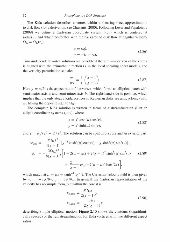
82 Protoplanetary Disk Structure
The Kida solution describes a vortex within a shearing-sheet approximationto disk flow (for a derivation, see Chavanis, 2000). Following Lesur and Papaloizou(2009) we define a Cartesian coordinate system (x,y) which is centered atradius r0 and which co-rotates with the background disk flow at angular velocity�K = �K(r0),
x = r0φ,
y = −(r − r0).(2.86)
Time-independent vortex solutions are possible if the semi-major axis of the vortexis aligned with the azimuthal direction (x in the local shearing sheet model), andthe vorticity perturbation satisfies
ωv
ωK= 1
χ
(χ + 1
χ − 1
). (2.87)
Here χ = a/b is the aspect ratio of the vortex, which forms an elliptical patch withsemi-major axis a and semi-minor axis b. The right-hand-side is positive, whichimplies that the only steady Kida vortices in Keplerian disks are anticyclonic (withωv having the opposite sign to �K).
The complete Kida solution is written in terms of a streamfunction ψ in anelliptic coordinate systems (μ,ν), where
x = f cosh(μ) cos(ν),
y = f sinh(μ) sin(ν),(2.88)
and f = a√
(χ2 − 1)/χ2. The solution can be split into a core and an exterior part,
ψcore = − 3�Kf 2
4(χ − 1)
[χ−1 cosh2(μ) cos2(ν) + χ sinh2(μ) sin2(ν)
],
ψext = − 3�Kf 2
8(χ − 1)2
[1 + 2(μ − μ0) + 2(χ − 1)2 sinh2(μ) sin2(ν) (2.89)
+ χ − 1
χ + 1exp[−2(μ − μ0)] cos(2ν)
],
which match at μ = μ0 = tanh−1(χ−1). The Cartesian velocity field is then givenby vx = −∂ψ/∂y,vy = ∂ψ/∂x. In general the Cartesian representation of thevelocity has no simple form, but within the core it is
vx,core = 3�Kχ
2(χ − 1)y,
vy,core = − 3�K
2χ(χ − 1)x,
(2.90)
describing simple elliptical motion. Figure 2.10 shows the contours (logarithmi-cally spaced) of the full streamfunction for Kida vortices with two different aspectratios.

2.9 Disk Large-Scale Structure 83
Figure 2.10 Contours showing the steady-state Kida vortex streamfunction fordifferent values of the vortex aspect ratio (top, a/b = 3, bottom, a/b = 1.5). Thesolution has an elliptical core that merges smoothly into the shear flow of the diskfurther out.
Vortices are extremely stable structures in two-dimensional fluid flows with sim-ple equations of state (for example, barotropic disks in which the pressure is solelya function of density) and little dissipation. They exhibit dynamics characteristic ofan inverse cascade of turbulent energy, in which multiple small vortices at initiallysimilar radii eventually merge to form a single large vortex. In realistic disk models,dissipative processes and the effects of the third dimension mean that vortices areexpected to be quasi-stable structures with a long but finite lifetime. Observedstructure in disks, if it is to be associated with the trapping of solid particles inthe high pressure cores of vortices, therefore likely requires a mechanism that isable to generate vortices in addition to the vorticity perturbations that would havebeen present during disk formation.
2.9.3 Ice Lines
Zonal flows and vortices are examples of hydrodynamic structures that can, inprinciple, form and persist within disks across a wide range of radii. A differenttype of observable structure may be associated to changes in the chemical makeupor size distribution of small solid particles in the vicinity of the water snow line
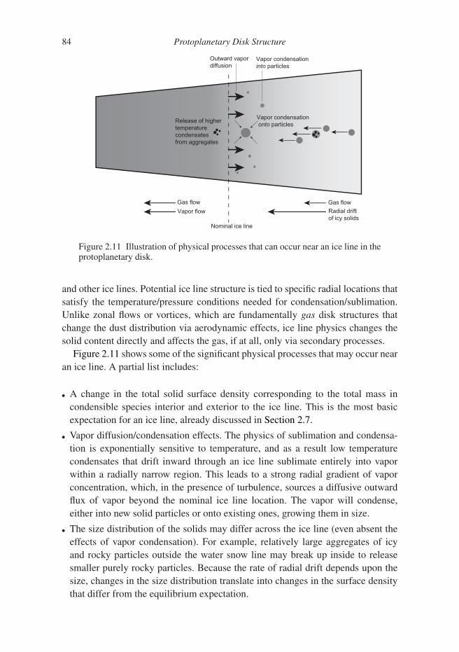
84 Protoplanetary Disk Structure
Nominal ice line
Gas flowVapor flow
Gas flowRadial driftof icy solids
Outward vapordiffusion
Vapor condensationinto particles
Vapor condensationonto particlesRelease of higher
temperature condensates from aggregates
Figure 2.11 Illustration of physical processes that can occur near an ice line in theprotoplanetary disk.
and other ice lines. Potential ice line structure is tied to specific radial locations thatsatisfy the temperature/pressure conditions needed for condensation/sublimation.Unlike zonal flows or vortices, which are fundamentally gas disk structures thatchange the dust distribution via aerodynamic effects, ice line physics changes thesolid content directly and affects the gas, if at all, only via secondary processes.
Figure 2.11 shows some of the significant physical processes that may occur nearan ice line. A partial list includes:
• A change in the total solid surface density corresponding to the total mass incondensible species interior and exterior to the ice line. This is the most basicexpectation for an ice line, already discussed in Section 2.7.
• Vapor diffusion/condensation effects. The physics of sublimation and condensa-tion is exponentially sensitive to temperature, and as a result low temperaturecondensates that drift inward through an ice line sublimate entirely into vaporwithin a radially narrow region. This leads to a strong radial gradient of vaporconcentration, which, in the presence of turbulence, sources a diffusive outwardflux of vapor beyond the nominal ice line location. The vapor will condense,either into new solid particles or onto existing ones, growing them in size.
• The size distribution of the solids may differ across the ice line (even absent theeffects of vapor condensation). For example, relatively large aggregates of icyand rocky particles outside the water snow line may break up inside to releasesmaller purely rocky particles. Because the rate of radial drift depends upon thesize, changes in the size distribution translate into changes in the surface densitythat differ from the equilibrium expectation.
2.10 Further Reading 85
Models incorporating some of the above effects have been developed (e.g. Steven-son & Lunine, 1988; Ros & Johansen, 2013; Pinilla et al., 2017). Strong effects,which could have a substantial impact on multiple phases of planet formation, arelikely to occur around the water snow line (and potentially also at the silicate “ice”line). Observable effects, of uncertain magnitude, are possible around the lowertemperature ice lines further out.
2.10 Further Reading
“Protoplanetary Disks and Their Evolution,” J. P. Williams & L. A. Cieza (2011), AnnualReview of Astronomy and Astrophysics, 49, 67.
“Models of the Structure and Evolution of Protoplanetary Disks,” C. P. Dullemond, D.Hollenbach, I. Kamp, & P. D’Alessio in Protostars and Planets V (2007), B. Reipurth,D. Jewitt, & K. Keil (eds.), Tucson: University of Arizona Press.
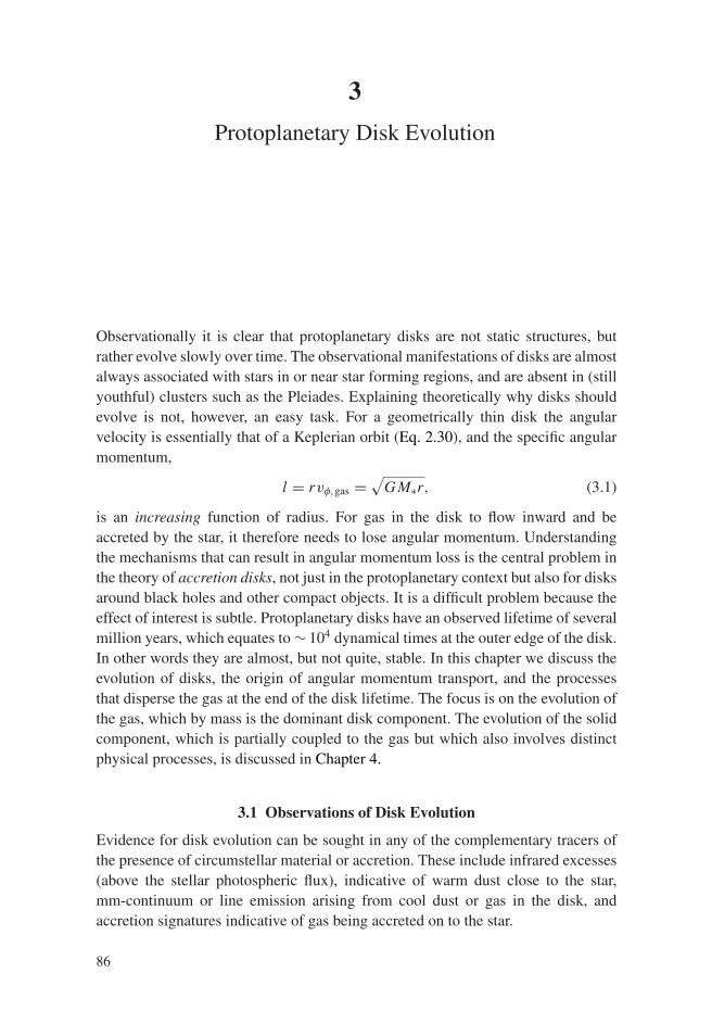
3
Protoplanetary Disk Evolution
Observationally it is clear that protoplanetary disks are not static structures, butrather evolve slowly over time. The observational manifestations of disks are almostalways associated with stars in or near star forming regions, and are absent in (stillyouthful) clusters such as the Pleiades. Explaining theoretically why disks shouldevolve is not, however, an easy task. For a geometrically thin disk the angularvelocity is essentially that of a Keplerian orbit (Eq. 2.30), and the specific angularmomentum,
l = rvφ,gas =√
GM∗r, (3.1)
is an increasing function of radius. For gas in the disk to flow inward and beaccreted by the star, it therefore needs to lose angular momentum. Understandingthe mechanisms that can result in angular momentum loss is the central problem inthe theory of accretion disks, not just in the protoplanetary context but also for disksaround black holes and other compact objects. It is a difficult problem because theeffect of interest is subtle. Protoplanetary disks have an observed lifetime of severalmillion years, which equates to ∼ 104 dynamical times at the outer edge of the disk.In other words they are almost, but not quite, stable. In this chapter we discuss theevolution of disks, the origin of angular momentum transport, and the processesthat disperse the gas at the end of the disk lifetime. The focus is on the evolution ofthe gas, which by mass is the dominant disk component. The evolution of the solidcomponent, which is partially coupled to the gas but which also involves distinctphysical processes, is discussed in Chapter 4.
3.1 Observations of Disk Evolution
Evidence for disk evolution can be sought in any of the complementary tracers ofthe presence of circumstellar material or accretion. These include infrared excesses(above the stellar photospheric flux), indicative of warm dust close to the star,mm-continuum or line emission arising from cool dust or gas in the disk, andaccretion signatures indicative of gas being accreted on to the star.
86
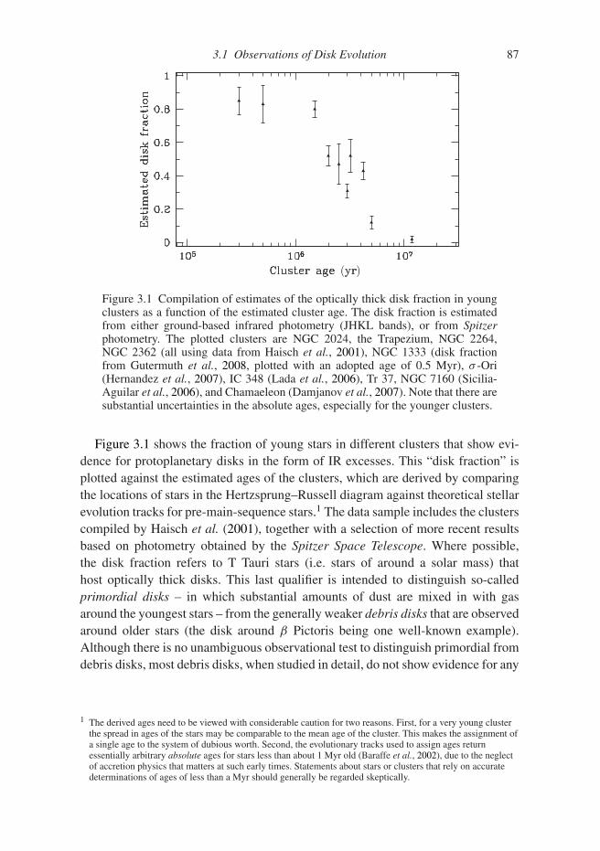
3.1 Observations of Disk Evolution 87
Figure 3.1 Compilation of estimates of the optically thick disk fraction in youngclusters as a function of the estimated cluster age. The disk fraction is estimatedfrom either ground-based infrared photometry (JHKL bands), or from Spitzerphotometry. The plotted clusters are NGC 2024, the Trapezium, NGC 2264,NGC 2362 (all using data from Haisch et al., 2001), NGC 1333 (disk fractionfrom Gutermuth et al., 2008, plotted with an adopted age of 0.5 Myr), σ -Ori(Hernandez et al., 2007), IC 348 (Lada et al., 2006), Tr 37, NGC 7160 (Sicilia-Aguilar et al., 2006), and Chamaeleon (Damjanov et al., 2007). Note that there aresubstantial uncertainties in the absolute ages, especially for the younger clusters.
Figure 3.1 shows the fraction of young stars in different clusters that show evi-dence for protoplanetary disks in the form of IR excesses. This “disk fraction” isplotted against the estimated ages of the clusters, which are derived by comparingthe locations of stars in the Hertzsprung–Russell diagram against theoretical stellarevolution tracks for pre-main-sequence stars.1 The data sample includes the clusterscompiled by Haisch et al. (2001), together with a selection of more recent resultsbased on photometry obtained by the Spitzer Space Telescope. Where possible,the disk fraction refers to T Tauri stars (i.e. stars of around a solar mass) thathost optically thick disks. This last qualifier is intended to distinguish so-calledprimordial disks – in which substantial amounts of dust are mixed in with gasaround the youngest stars – from the generally weaker debris disks that are observedaround older stars (the disk around β Pictoris being one well-known example).Although there is no unambiguous observational test to distinguish primordial fromdebris disks, most debris disks, when studied in detail, do not show evidence for any
1 The derived ages need to be viewed with considerable caution for two reasons. First, for a very young clusterthe spread in ages of the stars may be comparable to the mean age of the cluster. This makes the assignment ofa single age to the system of dubious worth. Second, the evolutionary tracks used to assign ages returnessentially arbitrary absolute ages for stars less than about 1 Myr old (Baraffe et al., 2002), due to the neglectof accretion physics that matters at such early times. Statements about stars or clusters that rely on accuratedeterminations of ages of less than a Myr should generally be regarded skeptically.

88 Protoplanetary Disk Evolution
significant gaseous component. The dust in these debris disks arises from erosivecollisions between larger solid bodies.
The infrared excess measurements of disk frequency provide a robust measure ofdisk evolution. The disk frequency is close to 100% for clusters whose mean stellarage is less than about 1 Myr. For older clusters, the disk frequency drops steadily,reaching 50% at around 3 Myr and falling almost to zero by about 6 Myr. Evidencefor primordial disks is essentially completely absent for stars of age 10 Myr orabove. From these observations, one infers a disk lifetime of about 3–5 Myr.
Strictly speaking, the aforementioned constraint on the “disk lifetime” refersonly to the survival time of small dust grains in the innermost (∼1 AU) regionof the disk. Does the disk as a whole evolve on the same time scale? Somewhatsurprisingly, there is evidence that it may. First, the accretion rate of gas onto the star – measured entirely independently via spectroscopic observationsof the hot continuum radiation produced when infalling gas impacts the stellarsurface – decays with time on a similar time scale (Hartmann et al., 1998). Second,the presence of one disk signature (such as an IR excess) usually, though notinvariably, implies that the other signatures (such as a mm excess) are also present,even when the different signatures arise at very different disk radii. This observationimplies that disks are dispersed across a range of radii on a relatively short timescale (Skrutskie et al., 1990; Wolk & Walter, 1996; Andrews & Williams, 2005).We will discuss further the import of this observation for models of disk dispersal,but for now we note only that it makes the assignment of a single lifetime for thedisk a meaningful concept.
3.2 Surface Density Evolution of a Thin Disk
Consider an axisymmetric protoplanetary disk whose gas surface density profileis given by �(r,t). We assume that the radial velocity vr(r,t) of gas in the diskis small,2 and note that the fact that the disk is geometrically thin (h/r 1)implies that the predominant forces at work are rotational support and gravity(cf. Section 2.4). If the potential is time independent, local conservation of angularmomentum implies that in the absence of angular momentum transport or loss�(r,t) cannot change with time. Accretion and disk evolution will occur in thepresence of angular momentum transport (often described as “viscosity,” or, evenmore loosely, as “friction”), which allows local parcels of gas to reduce their angu-lar momentum and spiral toward the star (global angular momentum conservationimplies, of course, that gas elsewhere in the disk must gain angular momentum andmove outward). This redistribution of angular momentum due to stresses withinthe disk is quite distinct from angular momentum loss – due for example to a
2 The radial velocity is defined such that vr < 0 corresponds to inflow.
3.2 Surface Density Evolution of a Thin Disk 89
magnetically driven outflow from the disk surface – and the evolution of disks underthe action of winds is different from that due to internal redistribution.
The qualitative evolution of disks in the presence of dissipative processeswas understood in the 1920s by, among others, the well-known geophysicist andastronomer Harold Jeffreys. The modern theory of thin disks was described in now-classic papers by Shakura and Sunyaev (1973) and Lynden-Bell and Pringle (1974).This theory is not fully predictive as it largely bypasses the central question of howefficiently angular momentum is transported within a disk flow, but it nonethelessforms the indispensable core to any discussion of disk evolution.
The evolution of �(r,t) can be derived by considering the continuity equation(expressing the conservation of mass) and the azimuthal component of the momen-tum equation (expressing angular momentum conservation). The rate of change ofthe mass within an annulus in the disk extending between r and r + �r is given by
∂
∂t(2πr�r�) = 2πr�(r)vr(r) − 2π(r + �r)�(r + �r)vr(r + �r). (3.2)
Writing for example �(r + �r) = �(r) + (∂�/∂r)�r , and taking the limit forsmall �r , the continuity equation yields
r∂�
∂t+ ∂
∂r(r�vr) = 0. (3.3)
Following the same procedure (e.g. Pringle, 1981) conservation of angular momen-tum gives
r∂
∂t
(r2��
) + ∂
∂r
(r2� · r�vr
) = 1
2π
∂G
∂r, (3.4)
where �, the angular velocity of the gas in the disk, is at this point unspecified andneed not be the Keplerian angular velocity due to a point mass. The rate of changeof angular momentum in the disk is determined by the change in surface densitydue to radial flows (the second term on the left-hand-side) and by the differencein the torque exerted on an annulus by stresses at the inner and outer edges. For aviscous fluid, the torque G can be written in the form
G = 2πr · ν�rd�
dr· r, (3.5)
where ν is the kinematic viscosity. The torque on an annulus is the product of thecircumference, the viscous force per unit length, and the lever arm r , and is pro-portional to the gradient of the angular velocity. Note that this dependence, whichis characteristic of a viscous fluid, is only an assumption if the “viscosity” is not atrue microscopic process but rather an effective viscosity resulting from turbulence.Proceeding, we eliminate vr between Eq. (3.3) and Eq. (3.4) and specialize to aKeplerian potential for which � ∝ r−3/2. We then obtain the evolution equation for

90 Protoplanetary Disk Evolution
the surface density of a geometrically thin disk under the action of internal angularmomentum transport:
∂�
∂t= 3
r
∂
∂r
[r1/2 ∂
∂r
(ν�r1/2
)]. (3.6)
The evolution equation is a diffusive partial differential equation for the surfacedensity �(r,t). It is linear if the viscosity ν is not itself a function of �. The equa-tion can also be derived directly from the Navier–Stokes equations for a viscousfluid in cylindrical polar coordinates.
3.2.1 The Viscous Time Scale
The diffusive form of Eq. (3.6) can be made more transparent with a change ofvariables. Defining
X ≡ 2r1/2, (3.7)
f ≡ 3
2�X, (3.8)
and assuming that the viscosity ν is a constant, the evolution equation takes theprototypical form of a diffusion equation,
∂f
∂t= D
∂2f
∂X2, (3.9)
with a diffusion coefficient D given by
D = 12ν
X2. (3.10)
Apart from its pedagogical value, this version of the evolution equation can beuseful numerically, since even naive finite difference schemes preserve conservedquantities accurately when the equation is cast in this form. The diffusion time scaleacross a scale �X implied by Eq. (3.9) is just (�X)2/D. Converting back to thephysical variables, we then find that the time scale on which viscosity will smoothout surface density gradients on a radial scale �r is
τν ∼ (�r)2
ν. (3.11)
If the disk has a characteristic size r , the surface density at all radii will evolve ona time scale
τν ≈ r2
ν. (3.12)
This last time scale is described as the viscous time scale of the disk. It can beestimated observationally by measuring, for example, the rate at which accretion

3.2 Surface Density Evolution of a Thin Disk 91
on to the star decays as a function of stellar age. For protoplanetary disks aroundsolar-type stars it appears to be of the order of a million years.
3.2.2 Solutions to the Disk Evolution Equation
A steady-state solution to Eq. (3.6) can be derived by setting ∂/∂t = 0 and inte-grating the resultant ordinary differential equation for the surface density. Applyingthe requisite boundary conditions is easiest if we start with the angular momentumconservation equation (Eq. 3.4) which does not assume Keplerian angular velocity.Setting the time derivative to zero and integrating, we have
2πr�vr · r2� = 2πr3ν�d�
dr+ constant. (3.13)
Noting that the mass accretion rate M = −2πr�vr we can write this equation inthe form
−M · r2� = 2πr3ν�d�
dr+ constant, (3.14)
where the constant of integration, which has the form of an angular momentumflux, remains to be determined. To specify the constant, we note that at a location inthe disk where d�/dr = 0 the viscous stress vanishes, and the constant is simplyequal to the flux of angular momentum advected inward along with the mass,
constant = −M · r2�. (3.15)
A simple case to consider is that where the protoplanetary disk extends all theway down to the surface of a nonrotating (or slowly rotating) star. The disk andthe star form a single fluid system, and the angular velocity (shown schematicallyin Fig. 3.2) must make a continuous transition between � = 0 in the star and� ∝ r−3/2 within the disk. The viscous stress vanishes at a radius R∗+rbl, where rbl
is the width of the boundary layer that separates the star from the Keplerian part ofthe disk. Within the boundary layer the angular velocity increases with radius, andthe sub-Keplerian rotational support cannot balance the inward gravitational force.
The hydrodynamics (and magnetohydrodynamics) of protoplanetary disk bound-ary layers is quite complex, and the flow structure in this region remains ratheruncertain. Elementary arguments, however, suggest that in most cases the radialextent of the boundary layer is a small fraction of the stellar radius. If magneticfields and viscosity are negligible, the momentum equation (Eq. 2.27) in axisym-metry can be written as
v2φ,gas
r= GM∗
r2+ 1
ρ
dP
dr+ vr
dvr
dr, (3.16)
92 Protoplanetary Disk Evolution
r
W
r = R*
dW / dr = 0
Keplerianangular velocity
W*
rbl
Figure 3.2 Schematic illustration of the angular velocity profile in a disk thatextends to the equator of a slowly rotating star. The viscous stress vanishes ata radial location r = R∗ + rbl where � has a maximum.
where P is the pressure. In the boundary layer – unlike in the disk itself – the rota-tional support (the term on the left-hand-side) cannot balance gravity. If, instead,radial pressure forces counteract the force of gravity,3 we require that
1
ρ
dP
dr∼ c2
s
rbl∼ �2
Kr, (3.17)
where cs is some characteristic sound speed in the boundary layer region and �K isthe Keplerian angular velocity. Recalling that the vertical scale-height h = cs/�K
we find that
rbl
r∼
(h
r
)2
. (3.18)
Provided that the boundary layer (like the disk) is geometrically thin, we concludethat force balance mandates that the radial extent of the boundary layer must alsobe narrow.
We are now in a position to evaluate the constant in Eq. (3.14). For a narrowboundary layer, R∗ + rbl � R∗ and the maximum in � occurs close to the stellarsurface. We have that
constant � −MR2∗
√GM∗R3∗
, (3.19)
and the steady-state solution for the disk (within which the angular velocity isKeplerian) simplifies to
3 Similar arguments apply if we consider the influence of the vrdvr/dr term rather than the pressure term, sincecausality requires that vr be subsonic.

3.2 Surface Density Evolution of a Thin Disk 93
ν� = M
3π
(1 −
√R∗r
). (3.20)
Once the viscosity is specified, this equation gives the steady-state surface densityprofile of a protoplanetary disk with a constant accretion rate M . Away from theinner boundary one notes that �(r) ∝ ν−1.
The solution given by Eq. (3.20) gives the surface density profile for a steadydisk subject to a zero-torque boundary condition at the inner edge. Physically, thisboundary condition is at least approximately realized for disks that extend to theequator of a slowly rotating star, and it is also the traditional choice in the moreexotic circumstance of a disk of gas around a black hole. In classical T Tauri starsit is often the case that stellar magnetic fields truncate the disk before it reachesthe stellar surface, and the resulting magnetic coupling between the star and theinner disk can violate the zero-torque assumption. More generally, one should notethat the turnover in the surface density profile at small radii implied by Eq. (3.20)reflects the fact that for a Keplerian flow the only way in which the torque canvanish is if the surface density goes to zero. The turnover is therefore a purelyformal result – in a real disk with a boundary layer the physical reason why thetorque vanishes is because of the existence of a maximum in �(r) – and the innerboundary condition needs to be considered carefully if one needs the detailed formof the surface density very close to the inner edge of the disk.
Time-dependent analytic solutions to Eq. (3.6) can be derived for a numberof simple forms for the viscosity and, although these forms are not particularlyrealistic for protoplanetary disks, the resulting solutions suffice to illustrate theessential behavior implied by the disk evolution equation. If ν = constant, a Green’sfunction solution to the evolution equation is possible.4 Suppose that at t = 0, allof the gas lies in a thin ring of mass m at radius r0,
�(r,t = 0) = m
2πr0δ(r − r0), (3.21)
where δ(r − r0) is a Dirac delta function. Given boundary conditions that imposezero torque at r = 0 and allow for free expansion toward r = ∞ the solution is(Lynden-Bell & Pringle, 1974)
�(x,τ) = m
πr20
1
τx−1/4 exp
[−(1 + x2)
τ
]I1/4
(2x
τ
), (3.22)
where we have written the solution in terms of dimensionless variablesx ≡ r/r0,τ ≡ 12νr−2
0 t , and I1/4 is a modified Bessel function of the firstkind. Since the evolution equation is linear for ν = f (r), the time-dependentsolution for arbitrary initial conditions can formally be written as a superpositionof these solutions. Although this approach is rarely illuminating, the solution
4 Related solutions are known for the more general situation in which ν is a power-law in radius.

94 Protoplanetary Disk Evolution
Figure 3.3 The Green’s function solution to the disk evolution equation withν = constant, showing the spreading of a ring of mass initially orbiting at r = r0.From top down the curves show the behavior as a function of the scaled time vari-able τ = 12νr−2
0 t , for τ = 0.004, τ = 0.008, τ = 0.016, τ = 0.032, τ = 0.064,τ = 0.128, and τ = 0.256.
(Eq. 3.22), which is plotted in Fig. 3.3, illustrates several generic features of diskevolution. As t increases the initially narrow ring spreads diffusively, with the massflowing toward r = 0 while simultaneously the angular momentum is carried bya negligible fraction of the mass toward r = ∞. This segregation of mass andangular momentum is a general feature of the evolution of a viscous disk, and isnecessary if accretion is to proceed without overall angular momentum loss fromthe system.
Often of greater practical utility than the Green’s function solution is the self-similar solution also derived by Lynden-Bell and Pringle (1974). Consider a disk inwhich the viscosity can be approximated as a power-law in radius,
ν ∝ rγ . (3.23)
Suppose that the disk at time t = 0 has the surface density profile corresponding toa steady-state solution (with this viscosity law) out to r = r1, with an exponentialcut-off at larger radii. Specifically, the initial surface density has the form
�(t = 0) = C
3πν1rγexp
[−r (2−γ )], (3.24)
where C is a normalization constant, r ≡ r/r1, and ν1 ≡ ν(r1). The self-similarsolution is then
�(r,T ) = C
3πν1rγT −(5/2−γ )/(2−γ ) exp
[− r (2−γ )
T
], (3.25)

3.2 Surface Density Evolution of a Thin Disk 95
Figure 3.4 The self-similar solution to the disk evolution equation is plotted fora viscosity ν ∝ r . The initial surface density tracks the profile for a steady-statedisk (� ∝ r−1, Eq. 3.20) at small radius, before cutting off exponentially beyondr = r1. The curves show the surface density at the initial value of the scaled timeT = 1, and at subsequent times T = 2, T = 4, and T = 8.
where
T ≡ t
ts+ 1, (3.26)
ts ≡ 1
3(2 − γ )2
r21
ν1. (3.27)
The evolution of related quantities such as the disk mass and accretion rate canreadily be derived from the above expression for the surface density. The solution isplotted in Fig. 3.4. Over time, the disk mass decreases while the characteristic scaleof the disk (initially r1) expands to conserve angular momentum. This solutioncan be useful both for studying evolving disks analytically, and for comparingobservations of disk masses, accretion rates, or radii with theory.
3.2.3 Temperature Profile of Accreting Disks
The radial dependence of the effective temperature of an actively accreting diskcan be derived by considering the net torque on a ring of width �r . This torque –(∂G/∂r)�r – does work at a rate
�∂G
∂r�r ≡
[∂
∂r(G�) − G�′
]�r, (3.28)
where �′ = d�/dr . Written this way, we note that if we consider the whole disk(by integrating over r) the first term on the right-hand-side is determined solely bythe boundary values of G�. We therefore identify this term with the transport of

96 Protoplanetary Disk Evolution
energy, associated with the viscous torque, through the annulus. The second term,on the other hand, represents the rate of loss of energy to the gas. We assume thatthis is ultimately converted into heat and radiated, so that the dissipation rate perunit surface area of the disk (allowing that the disk has two sides) is
D(r) = G�′
4πr= 9
8�2, (3.29)
where we have assumed a Keplerian angular velocity profile. For blackbody emis-sion D(r) = σT 4
disk. Substituting for �, and for ν� using the steady-state solutiongiven by Eq. (3.20), we obtain
T 4disk = 3GM∗M
8πσr3
(1 −
√R∗r
). (3.30)
We note that apart from near the inner boundary (r � R∗) the temperature profileof an actively accreting disk is Tdisk ∝ r−3/4. This has the same form as for a razor-thin disk that reprocesses stellar radiation (Eq. 2.40). Moreover, the temperatureprofile does not depend upon the viscosity. This is an attractive feature of the theorygiven that there are uncertainties regarding the origin and efficiency of disk angularmomentum transport, though it also eliminates many possible routes to learningabout the physics underlying ν via observations of steady disks.
Substituting a representative value of M = 10−7 M� yr−1 for the accretion rate,we obtain for a solar mass star at 1 AU an effective temperature Tdisk = 150 K.This is the surface temperature; as we will show shortly the central temperature ispredicted to be substantially higher.
3.3 Vertical Structure of Protoplanetary Disks
In an actively accreting disk it is intuitively plausible that the dissipation of gravi-tational potential energy into heat will be concentrated close to the disk mid-planewhere the density is highest. At most disk radii there is a large optical depth betweenthe surface and the mid-plane, so the heated gas cannot simply radiate directly tospace. Rather, energy will need to be transported vertically toward the photospherevia radiative diffusion or turbulent transport, and this requires that there exist atemperature gradient between z = 0 and the disk photosphere. Our goal here is tocalculate this gradient, and its effect on the vertical structure of the disk. This isdynamically important because – in simple models – the magnitude of the viscositythat controls the evolution depends upon the central conditions in the disk ratherthan those at the surface. Given a model for the viscosity and knowledge of thevertical structure we can then derive a (in principle) self-consistent model for thedisk structure and evolution.
The equations governing the vertical structure are essentially identical to thoseemployed in stellar structure calculations except for a change in the geometry
3.3 Vertical Structure of Protoplanetary Disks 97
from spherically symmetric to plane parallel. If energy transport is due to radiativediffusion, the equations to be solved are (a) hydrostatic equilibrium,
dP
dz= −ρgz, (3.31)
where gz is the vertical gravity (Eq. 2.15); (b) an equation describing the verticalvariation of the flux Fz,5
dFz
dz= 9
4ρν�2; (3.32)
and (c) the equation of radiative diffusion describing the relation between the fluxand the temperature gradient in an optically thick medium,
dT
dz= − 3κRρ
16σT 3Fz. (3.33)
These equations must be supplemented with an equation of state relating the pres-sure P to the fundamental variables ρ and T , with expressions for the Rosselandmean opacity κR, and with appropriate boundary conditions. The dependence ofthe viscosity on the local physical conditions is also required. If the resulting tem-perature gradient turns out to be steeper than the adiabatic gradient the disk isconvectively unstable, and the radiative flux needs to be supplemented with theconvective flux. This can be done in the usual manner using mixing length theory,or more crudely by simply setting the temperature gradient in convectively unstableregions equal to the adiabatic gradient. Given these ingredients, calculation of thedisk vertical structure is a straightforward numerical exercise.
3.3.1 The Central Temperature of Accreting Disks
An approximation to the vertical temperature structure can be derived under theassumption that the energy dissipation due to viscosity is strongly concentratedtoward z = 0. To proceed, we define the optical depth to the disk mid-plane:
τ = 1
2κR�, (3.34)
where κR is the Rosseland mean opacity and � is the disk surface density. Thevertical density profile of the disk is ρ(z). If the vertical energy transport occursvia radiative diffusion (in some regions convection may also be important), then forτ � 1 the vertical energy flux F(z) is given by the equation of radiative diffusion(Eq. 3.33 above):
Fz(z) = −16σT 3
3κRρ
dT
dz. (3.35)
5 For h r one may self-consistently assume that Fz � Fr , provided that the radial temperature profileremains smooth. The assumption of smoothness is violated if the disk is subject to thermal instabilities, but inthis case one should be wary of using time-independent vertical structure models in any case.
98 Protoplanetary Disk Evolution
Let us assume for simplicity that all of the energy dissipation occurs at z = 0. Inthat case Fz(z) = σT 4
disk is a constant with height. Integrating, assuming that theopacity is constant,
−16σ
3κR
∫ Tdisk
Tc
T 3dT = σT 4disk
∫ z
0ρ(z′)dz′, (3.36)
− 16
3κR
[T 4
4
]Tdisk
Tc
= T 4disk
�
2, (3.37)
where for the final equality we have used the fact that for τ � 1 almost all of thedisk gas lies below the photosphere. For large τ we expect that T 4
c � T 4disk, and the
equation simplifies to
T 4c
T 4disk
� 3
4τ . (3.38)
The implication of this result is that active disks with large optical depths aresubstantially hotter at the mid-plane than at the surface. For example, if atsome radius the optical depth to the disk’s thermal radiation is τ = 102, thenTc ≈ 3Tdisk. This is important since it is the central temperature that largelydetermines, for example, which ices or minerals can be present. Relatively modestlevels of accretion can thus affect the thermal and chemical structure of the disksubstantially.
It will often be the case that both stellar irradiation and accretional heatingcontribute significantly to the thermal balance of the disk. If we define Tdisk,visc
to be the effective temperature that would result from accretional heating in theabsence of irradiation (i.e. the quantity called Tdisk, with no subscript, above) andTirr similarly to be the irradiation-only effective temperature, then application ofEq. (3.37) yields
T 4c � 3
4τT 4
disk,visc + T 4irr, (3.39)
as an approximation for the central temperature, again valid for τ � 1. Note thatin disk models, such as those described in Section 2.5.4, in which the surface dusttemperature exceeds the local blackbody temperature, the fraction of the irradiatingflux that is thermalized within the disk is all that matters for the central tempera-ture. The temperature Tirr that enters into the above formula is then the “interior”temperature Ti computed for passive radiative equilibrium disk models.
3.3.2 Shakura–Sunyaev α Prescription
Although the effective temperature of an actively accreting disk (Eq. 3.30) is inde-pendent of the magnitude of the viscosity, the time scale on which evolution occurs(Eq. 3.11) and the profile of the surface density depend directly on the viscosity and

3.3 Vertical Structure of Protoplanetary Disks 99
its variation with radius. If we want to make progress in understanding the evolutionof disks we cannot evade discussion of the physical origin of angular momentumtransport forever! The first candidate to consider is molecular collisions, whichgenerate a viscosity in a shear flow because of the finite mean-free path λ in thegas. Molecular viscosity, which is the normal mechanism considered in terrestrialfluids modeled with the Navier–Stokes equations, is given, approximately, by
νm ∼ λcs, (3.40)
where the mean-free path in a gas with number density n is
λ = 1
nσmol. (3.41)
Here σmol is the cross-section for molecular collisions, which is very roughly equalto the physical size of molecules. Computing the molecular viscosity in detail is notat all a trifling task, but for our purposes high accuracy is not required, as an orderof magnitude estimate establishes that νm is far too small to matter in protoplanetarydisks. Adopting
σmol ≈ 2 × 10⁻¹⁵ cm2, (3.42)
as the collision cross-section of molecular hydrogen, and taking the sound speed at10 AU to be 0.5 km s−1 and the number density to be n = 1012 cm−3 we estimatethat νm ∼ 2.5 × 107 cm2 s−1. The implied viscous time scale (Eq. 3.11) is
tν � r2
νm= 3 × 10¹³ yr. (3.43)
This is approximately ten million times longer than the observed time scale for diskevolution. Molecular viscosity is not the source of angular momentum transportwithin disks.
The consequence of a small molecular viscosity is, of course, a large Reynoldsnumber, which can be defined as
Re ≡ UL
νm, (3.44)
where U and L are characteristic velocity and length scales in the system. TakingU = cs and L = h = 0.05r , the fluid Reynolds number at 10 AU is
Re ∼ 1010, (3.45)
a staggeringly large number! One concludes that in the presence of a physicalinstability the protoplanetary disk will be highly turbulent, with dissipation of fluidmotions occurring on a scale that is small compared to the disk scale-height.
Let us assume for the time being that the protoplanetary disk is turbulent. Theturbulent fluid motions will result in the macroscopic mixing of fluid elements atneighboring radii, which can act as an “effective” or “turbulent” viscosity. The

100 Protoplanetary Disk Evolution
magnitude of this turbulent viscosity can be estimated from dimensional arguments.If the turbulence is approximately isotropic, the outer scale of the turbulent flow islimited to be no larger than the smallest scale in the disk, which is generally the diskscale-height h. The velocity of the turbulent motions can be similarly limited to beno larger than the sound speed cs, since supersonic motions result in shocks andrapid dissipation (this is true even if the fluid is magnetized). We therefore write theturbulent viscosity in the form
ν = αcsh, (3.46)
where α is a dimensionless quantity, known as the Shakura–Sunyaev α parameter,that measures the efficiency of angular momentum transport due to turbulence(Shakura & Sunyaev, 1973).
With the help of Eq. (3.46) it is possible to specify the viscosity in terms oflocal disk quantities, the sound speed cs and the disk scale-height h, and therebycompute the local disk structure. We will follow this route shortly in Section 3.3.3.Before doing so, however, it is useful to note some of the limitations of any diskmodel constructed using the α prescription. First, the physical argument that wegave for Eq. (3.46) reasonably limits α to be less than unity, but does not give anybasis for assuming that α is a constant. We will take α to be constant later onlybecause it is impossible to proceed otherwise, not for any deeper reason. In fact,α may vary with the temperature, density, and composition of the disk gas, andthere may even be regions that fail to satisfy the basic assumption by not developingturbulence at all. Second, although the turbulent viscosity has the same dimensionsas a molecular viscosity, one should not forget that it arises from an entirely distinctphysical process. In particular, studying the evolution of turbulent disks in two orthree dimensions using the Navier–Stokes equations, valid for molecular viscosity,is not recommended.
3.3.3 Vertically Averaged Solutions
Using the α prescription we can compute the viscosity ν as a function of r,�,and α. This in turn determines the steady-state surface density profile �(r,α,M)
through Eq. (3.20), and can be employed together with Eq. (3.6) to calculate thetime-dependent evolution of an arbitrary initial surface density profile. Here wewill compute the viscosity in the vertically averaged or “one zone” approxima-tion. This approximation amounts to replacing the equation of radiative diffusion(Eq. 3.33) with the approximate result given as Eq. (3.38), and replacing the verticaldependence of all other quantities by their central values.
Consider an annulus of the disk with surface density � at a radius where theKeplerian angular velocity is � (in thin disk solutions r and M∗ enter only via thecombination � =
√GM∗/r3). The disk is characterized by eight variables: the
mid-plane temperature Tc, effective temperature Tdisk, sound speed cs, density ρ,

3.3 Vertical Structure of Protoplanetary Disks 101
vertical scale-height h, opacity κR, viscosity ν, and optical depth τ . Apart from theeffective temperature, which is defined at the photosphere, and the optical depth,which is evaluated between the surface and the mid-plane, all of these quantitiesare to be considered as the values at z = 0. Collecting together results that we haveeither already derived or which are trivial, we have the following set of equations:6
ν = αcsh, (3.47)
c2s = kBTc
μmp, (3.48)
ρ = 1√2π
�
h, (3.49)
h = cs
�, (3.50)
T 4c = 3
4τT 4
disk, (3.51)
τ = 1
2�κR, (3.52)
ν� = M
3π, (3.53)
σT 4disk = 9
8�2. (3.54)
Once the opacity κR(ρ,Tc) is specified, there are eight equations in eight unknownsto solve in order to determine the disk structure. If the opacity can be approximatedas a power-law in density and temperature the solution is analytic, and one obtainsan expression for ν that is a power-law in r,α, and �.
As an explicit example, we may consider a disk in which the mid-plane opacityis due to icy particles. In this limit an approximate form for the opacity is
κ = κ0T2
c , (3.55)
with the constant having a numerical value in cgs units κ0 = 2.4 × 10⁻⁴. For
this opacity there is no dependence on density, and hence the equation for ρ isredundant. Eliminating variables in turn the remaining equations yield
�3 = 64
81π
σ
κ0
(μmp
kB
)2
α−2M . (3.56)
6 For simplicity we assume that r � R∗ and neglect terms that depend upon the inner boundary conditions.Note also that different numerical factors can enter into, for example, the definition of the central density to beused in these equations. Given the overriding uncertainty that originates from our poor knowledge of angularmomentum transport in disks, worrying about the “correct” value of such factors is rarely profitable.

102 Protoplanetary Disk Evolution
For an accretion rate M = 10−7 M� yr−1 and an α = 0.01, we find that
� ≈ 140 g cm−2. The corresponding viscosity is ν ≈ 5 × 1015 cm2 s−1, and theviscous time at 30 AU is about 1.3 × 10⁶ yr. This time scale is broadly consistentwith protoplanetary disks evolving significantly over a few million years, andindeed most observational attempts to constrain α via measures of disk evolutionreturn estimates α ∼ 10−2 (e.g. Hartmann et al., 1998).
3.4 Hydrodynamic Angular Momentum Transport
The Shakura–Sunyaev α prescription furnishes a formula for the viscosity butleaves unanswered some of the most basic questions. What is the origin of thepostulated turbulence? How large is α, and what is its dependence (if any) on thephysical conditions within the disk? These issues are at the forefront of researchfor protoplanetary disks and for other accreting systems.
For disks, such as those around black holes, in which the gas is well coupledto the magnetic field, the physical origin of turbulence is well understood. Themagnetorotational instability (MRI), which we discuss in Section 3.5.1, operatesefficiently under such conditions and generates vigorous, sustained, turbulencewhich transports angular momentum outward. Other hydrodynamic processes(such as convection) may modify the properties of the turbulence, and magnetizeddisk winds may even be more important in driving accretion, but turbulent accretionwould occur even in their absence.
Protoplanetary disks are more complex and interesting. There are substantialregions within protoplanetary disks where the ionization fraction is so low that themagnetic field is effectively decoupled from the fluid dynamics of the gas. Underlow ionization conditions the MRI does not operate in the same way as it does inideal MHD, and the strength of turbulence and angular momentum transport canbe heavily suppressed. It is then possible, but not guaranteed, that hydrodynamicprocesses generate the bulk of whatever turbulence and transport is present. Thesimplest disk flows are linearly stable, but there are loopholes if the disk has non-trivial radial or vertical structure, or a large mass, which allow purely hydrodynamicsources of turbulence.
3.4.1 The Rayleigh Criterion
The stability of a rotating flow to infinitesimal hydrodynamic perturbations can bederived by linearizing the fluid equations, setting the time dependence of perturba-tions to be proportional to eiωt , and searching for exponentially growing or decayingmodes for which ω is imaginary. For a nonmagnetized, non-self-gravitating disk(roughly speaking, one for which Mdisk/M∗ < h/r) the appropriate stability criteriaare due to Rayleigh (for a derivation see e.g. Pringle & King, 2007). Such a disk

3.4 Hydrodynamic Angular Momentum Transport 103
flow is linearly stable to axisymmetric perturbations if and only if the specificangular momentum increases with radius. For instability we require
dl
dr= d
dr
(r2�
)< 0. (3.57)
In a Keplerian disk the specific angular momentum is an increasing function ofradius, l ∝ √
r (Eq. 3.1), and the flow is predicted to be hydrodynamically stable.Despite the enormous value of the Reynolds number, there is then no ready justifi-cation for invoking hydrodynamic turbulence as the origin of the turbulent viscosityneeded to drive accretion.
The Rayleigh criterion is based upon a linear analysis, and says nothing aboutwhether a disk might be unstable to finite-amplitude perturbations. It is very dif-ficult to prove that a given hydrodynamic flow is non-linearly stable. Nonetheless,the results of both numerical and laboratory experiments (Hawley et al., 1999; Jiet al., 2006) support the view that the simplest hydrodynamic disk flow would beunable to sustain astrophysically relevant levels of turbulence. The use of the word“simplest” here is a very significant caveat. It implies a toy disk model in whichthere is no vertical stratification, no vertical shear, a stable radial entropy profile,and no self-gravity. Linear and nonlinear instabilities are known to exist when anyof these restrictions are relaxed.
3.4.2 Self-Gravity
Up to now we have considered disks whose own gravity is negligible comparedto the force from the central star. Such disks are axisymmetric, which impliesthat no torque is exerted on gas at one radius due to the gravitational force frommatter elsewhere in the disk. As the disk becomes more massive there is anincreasing tendency for its own self-gravity to result in the formation of over-dense “clumps.” Gravitational forces between these clumps can result in angularmomentum transport.
Self-gravity is an important potential mechanism for planetesimal formation,which is discussed in Chapter 4. We defer a formal mathematical analysis of theconditions for clump formation until then, in favor of a simple argument based ontime scales. Within a disk, the self-gravity of the disk gas always has a tendency toform denser clumps, but this is opposed by both pressure forces and by shear, whichtend to oppose clump formation. We can estimate the conditions under which self-gravity is strong enough to win out over these stabilizing effects by requiring thatthe time scale for collapse be shorter than the time scales on which sound wavescan cross a clump, or shear destroy it.
Consider a forming clump of scale �r and mass m ∼ π(�r)2�. In isolation,such a clump would collapse on the free-fall time scale

104 Protoplanetary Disk Evolution
tff ∼√
�r3
Gm∼
√�r
πG�. (3.58)
Stabilizing influences that may prevent collapse are pressure and shear. The timescale for a sound wave to cross the clump is
tp ∼ �r
cs, (3.59)
where cs is the disk sound speed, while the shear time scale (the time scale requiredfor a clump to be sheared azimuthally by an amount �r) is
tshear = 1
r
(d�
dr
)−1
∼ �−1. (3.60)
One observes that the shear time scale is independent of the clump size �r , whereasthe sound crossing time increases linearly with �r . Pressure tends to stabilize smallregions of the disk against gravitational collapse, while shear stabilizes the largestscales. The disk will be marginally unstable to clump formation if the free-fall timescale on the scale where shear and pressure support match is shorter than eithertp or tshear. Setting all three time scales equal, we obtain a condition for instabilityin the form
πG� >∼ cs�. (3.61)
At a given radius (i.e. at fixed �) the disk will be unstable if it is massive (large �)and/or cool and thin (small cs). A more formal analysis (Toomre, 1964) gives thesame result. The stability of a disk of either gas or stars is controlled by a parameter
Q ≡ cs�
πG�, (3.62)
known as the “Toomre Q” parameter.7 Instability of the disk against self-gravitysets in once Q <∼ 1. Using the fact that h = cs/�, and estimating the disk mass asMdisk ∼ πr2�, we can write the instability threshold in the more intuitive form
Mdisk
M∗>∼
h
r. (3.63)
This is (up to numerical factors) the same condition that we derived earlier(Eq. 2.24) for when disk gravity becomes important for the vertical structure.Since h/r ≈ 0.05 is a representative number for protoplanetary disks, we requirefairly massive disks before the effects of self-gravity can be expected to becomeimportant. Such disks are more likely to have existed at early epochs, possibly priorto the optically visible T Tauri phase of YSO evolution.
7 If the disk is extremely massive, then the angular velocity profile itself may depart significantly from theKeplerian form. In that case, � in the stability criterion must be replaced by the epicyclic frequency κ , definedvia κ2 = (1/r3)d(r4�2)/dr (note that κ = � for a Keplerian disk).

3.4 Hydrodynamic Angular Momentum Transport 105
If self-gravity sets in within a disk, there are two possible outcomes:
• Collapse may continue unhindered, destroying the disk and forming one or morebound objects. Disk fragmentation via this process is a mechanism for planetes-imal formation (in the case where the collapse occurs in the solid componentof the disk material) star or brown dwarf formation, and, perhaps, giant planetformation.
• Adiabatic heating as the clump contracts to higher density may yield enoughpressure to prevent complete collapse. Numerical simulations show that the out-come is the development of spiral arms induced by the self-gravity within thedisk. Gravitational forces set up by the spiral arms work to transport angularmomentum outward and mass inward.
The boundary between these possibilities is set by the ability of the disk to radiateaway its thermal energy. If the disk can cool on a short time scale, pressure cannotbuild up within contracting clumps, and fragmentation results. Slow cooling, whichis physically more likely in most protoplanetary disks, results instead in stableangular momentum transport.
A priori it is far from obvious that angular momentum transport via self-gravitycan be described using the local language of α disks that we have developedpreviously. If, however, one allows this sleight of hand, we can give a plausibleargument for an important result derived more formally by Gammie (2001): namelythat the equivalent α in a self-gravitating disk depends upon the cooling time ofthe gas. Let us assume that the disk does not fragment, in which case heating at alocal rate,
Q+ = 9
4�2, (3.64)
must on average balance cooling. If the disk is optically thick, the localcooling rate is
Q− = 2σT 4disk. (3.65)
Writing the “gravitational viscosity” in the form
ν = αgravc2
s
�= αgrav
�
kBTc
μmp, (3.66)
and setting Q+ = Q−, we find that the effective α depends upon the ratioσT 4
disk/(�Tc). We recognize this ratio as being proportional to the cooling ratefrom the disk surface divided by the thermal energy. We therefore define
tcool = U
2σT 4disk
, (3.67)

106 Protoplanetary Disk Evolution
where U is the thermal energy content of the disk gas per unit area. Noting that,approximately, U � cp�Tc, where cp is the heat capacity of the gas, the thermalbalance condition yields
αgrav ≈ 4
9γ (γ − 1)�tcool. (3.68)
In this expression γ is the two-dimensional adiabatic index (defined in termsof the two-dimensional pressure P and internal energy U via P = (γ − 1)U )and we have reinserted the correct numerical factors from the analysis by Gam-mie (2001). One finds that the strength of angular momentum transport fromself-gravity depends upon the cooling time of the disk, measured in units of thelocal dynamical time. This is intuitively reasonable. If the disk cools rapidly,strong gravitational turbulence, characterized by large density contrasts, is requiredin order to generate enough heat to balance the cooling. The strong densitycontrasts result in larger torques due to self-gravity. Eventually, if the coolingis too rapid, the disk cannot be stabilized against collapse, and fragmentationensues. Simulations show that stable angular momentum transport is possible onlyfor αgrav
<∼ 0.1.
3.4.3 Vertical Shear Instability
The vertical shear instability (VSI) is a linear hydrodynamic instability that can bepresent in disks whenever the angular velocity of the equilibrium structure varieswith height above the mid-plane. The instability, which is closely related to onestudied in rotating stars (Goldreich & Schubert, 1967; Fricke 1968), was suggestedas a possible source of disk turbulence by Urpin and Brandenburg (1998) andstudied in detail by Nelson et al. (2013).
Figure 3.5 illustrates the type of fluid perturbations that are unstable to the VSI.Let us assume for simplicity that the vertical structure of the disk is neutrallybuoyant, so that there is neither a driver of vertical motions (as would be the caseif the vertical entropy profile were convectively unstable) nor a stabilizing effect(as would be true for a highly stable stratification). In that limit the fluid stability isentirely determined by a Rayleigh-like criterion, and in the absence of vertical shearthe system is stable. In the presence of vertical shear, however, displacement of afluid element along a near-vertical trajectory from point “A” to point “B” moves itradially outward to a place where the specific angular momentum is lower. This isunstable. The general criterion for instability for a mode with radial wavenumberkr and vertical wavenumber kz,
∂l2
∂r− kr
kz
∂l2
∂z< 0, (3.69)
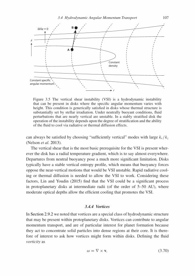
3.4 Hydrodynamic Angular Momentum Transport 107
Constant specific angular momentum
Constantdensity
δl/δz = 0
r
z
A
B
Figure 3.5 The vertical shear instability (VSI) is a hydrodynamic instabilitythat can be present in disks where the specific angular momentum varies withheight. This condition is generically satisfied in disks whose thermal structure issubstantially set by stellar irradiation. Under neutrally buoyant conditions, fluidperturbations that are nearly vertical are unstable. In a stably stratified disk theoperation of the instability depends upon the degree of stratification and the abilityof the fluid to cool via radiative or thermal diffusion effects.
can always be satisfied by choosing “sufficiently vertical” modes with large kr/kz
(Nelson et al. 2013).The vertical shear that is the most basic prerequisite for the VSI is present wher-
ever the disk has a radial temperature gradient, which is to say almost everywhere.Departures from neutral buoyancy pose a much more significant limitation. Diskstypically have a stable vertical entropy profile, which means that buoyancy forcesoppose the near-vertical motions that would be VSI unstable. Rapid radiative cool-ing or thermal diffusion is needed to allow the VSI to work. Considering thesefactors, Lin and Youdin (2015) find that the VSI could be a significant processin protoplanetary disks at intermediate radii (of the order of 5–50 AU), wheremoderate optical depths allow the efficient cooling that promotes the VSI.
3.4.4 Vortices
In Section 2.9.2 we noted that vortices are a special class of hydrodynamic structurethat may be present within protoplanetary disks. Vortices can contribute to angularmomentum transport, and are of particular interest for planet formation becausethey act to concentrate solid particles into dense regions at their core. It is there-fore of interest to ask how vortices might form within disks. Defining the fluidvorticity as
ω = ∇ × v, (3.70)
108 Protoplanetary Disk Evolution
we obtain an equation for the evolution of the vortensity ω/ρ by taking the curlof the momentum equation. In the absence of magnetic fields and microscopicviscosity, the result is
D
Dt
(ω
ρ
)=
(ω
ρ
)· ∇v − 1
ρ∇
(1
ρ
)× ∇P . (3.71)
This equation exposes the most important physical consideration concerning therole of vortices within protoplanetary disks. In a barotropic fluid (one in whichP = P(ρ) only) surfaces of equal pressure are always parallel to surfaces ofequal density. In this limit the second term on the right-hand-side vanishes, andany vortensity present within the disk is simply advected with the fluid motion.To the extent that the barotropic approximation is valid, vorticity is a conservedquantity that cannot be easily created, or, once present, destroyed. Indeed, intwo-dimensional models of protoplanetary disks, vortices are found to be stablelong-lived structures whose interactions can act to transport angular momentum8
(Godon & Livio, 1999; Johnson & Gammie, 2005).Vorticity can be spontaneously generated in more complete disk models, for
example as a consequence of the subcritical baroclinic instability(Petersen et al., 2007; Lesur & Papaloizou, 2010). This is a nonlinear (or “sub-critical”) instability that relies for its existence on the interplay of two distinctthermodynamic properties of the disk. First, it requires that the radial entropygradient in the disk be unstable to the Schwarzschild criterion for the onsetof convection. (This does not mean that convection sets in, because in a diskrotation exerts a strong stabilizing effect.) Second, radiative cooling (or thermaldiffusion) must occur at a rate that promotes the generation of vorticity. Thesepre-conditions (which can be expressed quantitatively) mean that the subcriticalbaroclinic instability, rather like the vertical shear instability, is a process whoseexistence and operation in disks is strongly dependent on the detailed disk structure.
The Rossby wave instability (RWI; Lovelace et al., 1999) is a second physicalmechanism for producing vortices within at least some protoplanetary disks. TheRWI is a linear instability that is present whenever there is “sufficiently sharp”radial structure in the disk. Specifically, for a two-dimensional disk model withangular velocity �(r), vertically integrated pressure P(r), and adiabatic index γ ,we can define the entropy S and epicyclic frequency κ via
S = P
�γ, (3.72)
κ2 = 1
r3
∂
∂r(r4�2). (3.73)
In terms of these quantities, the stability of the disk to the RWI is determined bythe radial profile of a generalized potential vorticity,
8 This is in accord with the observation that vortices can be long lived in strongly stratified, and thus physicallyquasi-two-dimensional, atmospheres. Jupiter’s Great Red Spot is a particularly spectacular example.

3.5 Magnetohydrodynamic Angular Momentum Transport 109
L(r) = ��
κ2× S2/γ . (3.74)
A necessary condition for RWI is that L have an extremum. A precise sufficientcondition is not easily stated, but variations in the potential vorticity of the order of10% over radial scales ≈ h suffice to trigger instability. Once triggered, the RWIleads to the formation of anticyclonic vortices on time scales of the order of 10�−1,which typically merge to form a single larger vortex on a longer time scale.
Localized radial structure can be produced in protoplanetary disks from thegravitational perturbation of a growing planet (see Section 7.1.4), and this is aspecific scenario that is theoretically expected to initiate RWI. The instability couldalso occur in disks that do not contain planets, if some (obviously nondiffusive)process was able to create relatively pronounced ring-like structures.
3.5 Magnetohydrodynamic Angular Momentum Transport
Coupling a magnetic field to the gas grants the fluid additional degrees of freedomthat violently destabilize the disk. The condition for a weakly magnetized disk flowto be linearly unstable is that the angular velocity (rather than the specific angularmomentum as in the fluid case) decrease with radius,
d
dr
(�2
)< 0, (3.75)
and this condition is satisfied by Keplerian disks. The linear instability of adisk coupled to a magnetic field is known as the magnetorotational (MRI) orBalbus–Hawley instability. The mathematical analysis of the instability has along history (Velikhov, 1959; Chandrasekhar, 1961) but its importance in thecontext of accretion disks was only recognized at a much later date (Balbus &Hawley, 1991). This long hiatus is something of a puzzle, as Chandrasekhar’s workwas published in his classic textbook Hydrodynamic and Hydromagnetic Stability.Indeed, Safronov (1969) came agonizingly close to recognizing the significance ofChandrasekhar’s result for the origin of turbulence within the protoplanetary disk.He noted correctly that the MHD stability criterion does not reduce to the Rayleighcriterion as the magnetic field tends toward zero, and that “for a weak magneticfield the cloud should be less stable than we found earlier in the absence of thefield.” Safronov then, however, dismisses the MRI on the (incorrect) grounds thatthe instability requires that the viscosity and diffusivity are identically zero.
3.5.1 Magnetorotational Instability
In the limit of ideal magnetohydrodynamics (MHD) the disk can be described bythe equations of continuity,
∂ρ
∂t+ ∇ · (ρv) = 0, (3.76)

110 Protoplanetary Disk Evolution
momentum conservation,
∂v∂t
+ (v · ∇) v = − 1
ρ∇
(P + B2
8π
)− ∇� + 1
4πρ(B · ∇) B, (3.77)
and magnetic induction,
∂B∂t
= ∇ × (v × B) . (3.78)
The symbols have their conventional meanings, ρ is the density, v is the velocity,B is the magnetic field, P is the pressure, B = |B|, and � is the gravitationalpotential. Magnetized disks have qualitatively different stability properties fromfluid disks because of the presence of magnetic tension (described by the third termon the right-hand-side of Eq. 3.77), which exerts a force on the fluid that attemptsto straighten curved field lines.
Demonstrating the existence of the MRI in the general case requires moderatelylengthy algebra, which can be found in the review by Balbus and Hawley (1998).The essence of the instability, however, lies in the interplay of magnetic tensionand flux freezing (Eq. 3.78) within a differentially rotating system, and this can bedemonstrated in much simpler model systems. Consider an axisymmetric, incom-pressible disk that is threaded by a vertical magnetic field. In cylindrical polarcoordinates (r,z,φ), the equations of motion of a small parcel of gas then read
r − rφ2 = −d�
dr+ fr, (3.79)
rφ + 2r φ = fφ, (3.80)
where the dots denote derivatives with respect to time, and fr and fφ are forcesdue to the coupling of the gas to the magnetic field, which we will specify shortly.We now concentrate attention on a small patch of the disk at radius r0, co-rotatingwith the overall orbital motion at angular velocity �. We define a local Cartesiancoordinate system (x,y) via
r = r0 + x, (3.81)
φ = �t + y
r0, (3.82)
and substitute these expressions into Eq. (3.80) above. Discarding quadratic terms,the result is
x − 2�y = −xd�2
d ln r+ fx,
y + 2�x = fy .(3.83)
The second term on the left-hand-side of these equations represents the Coriolisforce. In the absence of magnetic forces these equations describe the epicyclicmotion of pressureless fluid perturbed from an initially circular orbit.
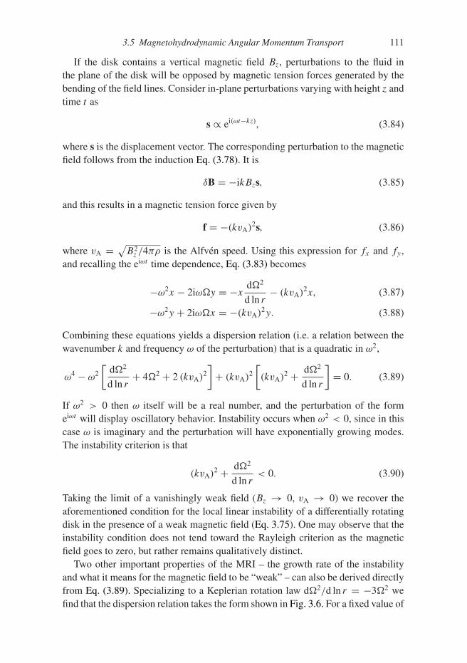
3.5 Magnetohydrodynamic Angular Momentum Transport 111
If the disk contains a vertical magnetic field Bz, perturbations to the fluid inthe plane of the disk will be opposed by magnetic tension forces generated by thebending of the field lines. Consider in-plane perturbations varying with height z andtime t as
s ∝ ei(ωt−kz), (3.84)
where s is the displacement vector. The corresponding perturbation to the magneticfield follows from the induction Eq. (3.78). It is
δB = −ikBzs, (3.85)
and this results in a magnetic tension force given by
f = −(kvA)2s, (3.86)
where vA = √B2
z /4πρ is the Alfven speed. Using this expression for fx and fy ,and recalling the eiωt time dependence, Eq. (3.83) becomes
−ω2x − 2iω�y = −xd�2
d ln r− (kvA)2x, (3.87)
−ω2y + 2iω�x = −(kvA)2y. (3.88)
Combining these equations yields a dispersion relation (i.e. a relation between thewavenumber k and frequency ω of the perturbation) that is a quadratic in ω2,
ω4 − ω2
[d�2
d ln r+ 4�2 + 2 (kvA)2
]+ (kvA)2
[(kvA)2 + d�2
d ln r
]= 0. (3.89)
If ω2 > 0 then ω itself will be a real number, and the perturbation of the formeiωt will display oscillatory behavior. Instability occurs when ω2 < 0, since in thiscase ω is imaginary and the perturbation will have exponentially growing modes.The instability criterion is that
(kvA)2 + d�2
d ln r< 0. (3.90)
Taking the limit of a vanishingly weak field (Bz → 0, vA → 0) we recover theaforementioned condition for the local linear instability of a differentially rotatingdisk in the presence of a weak magnetic field (Eq. 3.75). One may observe that theinstability condition does not tend toward the Rayleigh criterion as the magneticfield goes to zero, but rather remains qualitatively distinct.
Two other important properties of the MRI – the growth rate of the instabilityand what it means for the magnetic field to be “weak” – can also be derived directlyfrom Eq. (3.89). Specializing to a Keplerian rotation law d�2/d ln r = −3�2 wefind that the dispersion relation takes the form shown in Fig. 3.6. For a fixed value of
112 Protoplanetary Disk Evolution
Stable
Unstable
Figure 3.6 The unstable branch of the dispersion relation for the magnetorota-tional instability (Eq. 3.89) is plotted for a disk with a Keplerian angular velocityprofile. Both ω and kvA have been plotted scaled to the orbital frequency �. Theflow is unstable (ω2 < 0) for all spatial scales smaller than kvA <
√3� (rightmost
dashed vertical line). The most unstable scale (shown as the dashed vertical line atthe center of the plot) is kvA = (
√15/4)�.
the magnetic field strength (and hence a fixed Alfven speed vA) the flow is unstablefor wavenumbers k < kcrit (i.e. on sufficiently large spatial scales), where
kcritvA =√
3�. (3.91)
As the magnetic field becomes stronger, the smallest scale λ = 2π/kcrit that isunstable grows, until eventually it exceeds the disk’s vertical extent, which wemay approximate as 2h, where h is the scale-height. For stronger vertical fieldsno unstable MRI modes fit within the thickness of the disk, and the instability willbe suppressed. Noting that h = cs/�, we can express the condition that the verticalmagnetic field be weak enough to admit the MRI (i.e. that λ < 2h) as
B2 <12
πρc2
s, (3.92)
where cs is the disk sound speed. If we define the plasma β parameter as the ratioof gas to magnetic pressure,
β ≡ 8πP
B2, (3.93)
Eq. (3.92) can be expressed alternatively as
β >2π2
3. (3.94)
3.5 Magnetohydrodynamic Angular Momentum Transport 113
A magnetic field whose vertical component approaches equipartition with the ther-mal pressure (β ∼ 1) will therefore be too strong to admit the existence of linearMRI modes, but a wide range of weaker fields is acceptable.
The maximum growth rate can be determined by setting dω2/d(kvA) = 0 forthe unstable branch of the dispersion relation shown in Fig. 3.6. The most unstablescale for a Keplerian disk is
(kvA)max =√
15
4�, (3.95)
with a corresponding growth rate
|ωmax| = 3
4�. (3.96)
The main point to notice about this last result is that it implies an extremely vigorousgrowth of the instability, with an exponential growth time scale that is a fraction ofan orbital period. Practically, this means that if a disk is unstable to the MRI it ishard to envisage other physical processes that will operate on a shorter time scaleand prevent the MRI from dominating the evolution.
The physical origin of the MRI is fairly transparent for this simple configuration.Consider the effect of perturbing a weak vertical magnetic field threading an other-wise uniform disk, so that some fluid (tied to the magnetic field due to flux freezing)moves slightly inward and some slightly outward. Due to the differential rotation,the perturbed field line – which now connects adjacent annuli in the disk – will besheared by the differential rotation of the disk into a trailing spiral pattern. Providedthat the field is weak enough, magnetic tension is inadequate to snap the field linesback to the vertical. What tension there is, however, acts to reduce the angularmomentum of the inner fluid element, and boost that of the outer fluid element.The transfer of angular momentum further increases the separation, leading to aninstability.
The very rapid linear growth of the MRI implies, of course, that there is no phys-ical way to set up a disk with initial conditions that resemble those used for analyticconvenience above. Within a real disk it is the nonlinear properties of the instabilitythat are of interest for angular momentum transport, and these can only be studiedin detail via numerical MHD simulations. Disentangling physical from numericaleffects in such calculations is a nontrivial exercise, but one consensus result is thatthe nonlinear evolution of the MRI leads to a state of sustained MHD turbulencewhich is able to maintain disk magnetic fields in the presence of dissipation. Aflow with this property is described as a magnetic dynamo. Denoting the velocityfluctuations in the radial and azimuthal directions by δvr and δvφ respectively, wecan define an equivalent Shakura–Sunyaev α parameter in terms of an average overthe fluctuating velocity and magnetic fields:
α =⟨δvrδvφ
c2s
− BrBφ
4πρc2s
⟩, (3.97)
114 Protoplanetary Disk Evolution
where the angle brackets denote a density-weighted average over time. This for-mula provides a way to connect the small-scale flow dynamics seen in numericalsimulations with the gross angular momentum transport efficiency that is relevantfor the evolution of the disk as a whole. Numerical work shows that the magnetictransport term (the second term on the right-hand-side, described as the Maxwellstress) is generically much larger than the fluid (or Reynolds) contribution in MHDturbulent flows initiated by the MRI, although both terms are positive. The predictedmagnitude in the ideal MHD limit is of the order of α ∼ 10−2 if there is no netvertical magnetic field threading the disk, and higher if there is.
3.6 Effects of Partial Ionization and Dead Zones
In Section 2.8 we showed that the protoplanetary disk at the radii of greatest interestfor planet formation (0.1–50 AU) is expected to be predominantly neutral. Magneticfields, which couple to charged particles, affect the neutral component of the fluidindirectly, via collisions between charged and neutral species. Accounting fully forthe influence of partial ionization on the MRI (and, by extension, on the likelyproperties of disk turbulence and angular momentum transport) requires us to con-sider the role of three new physical effects that, together, make up non-ideal MHD:Ohmic diffusion, ambipolar diffusion, and the Hall effect.
3.6.1 Ohmic Dead Zones
A full analysis of the effect of the non-ideal terms on protoplanetary disks isquite involved, so it is useful to start with a deliberately oversimplified model thatincludes Ohmic diffusion only. The induction equation then takes the form
∂B
∂t= ∇ × [v × B − η∇ × B] , (3.98)
where v is the velocity of the neutral fluid and the second term on the right-hand-side represents the effect of Ohmic diffusion. The magnetic diffusivity, η, isinversely proportional to the electrical conductivity σc,
η = c2
4πσc. (3.99)
Under the assumption that the charge carriers in the disk are electrons and ions wecan write down an explicit expression for η. The electrical conductivity (and, hence,the magnetic diffusivity) is determined by collisions between electrons and neutralspecies. If the cross-section for such collisions is σ , the collision frequency is
νe = nn〈σv〉e, (3.100)

3.6 Effects of Partial Ionization and Dead Zones 115
where nn is the number density of neutrals and the brackets denote a velocity-weighted average. The conductivity is
σc = e2ne
meνe. (3.101)
Numerically, the collision rate is given by (Draine et al., 1983)
〈σv〉e = 8.28 × 10⁻¹⁰T 1/2 cm3 s−1. (3.102)
With this microphysical background we can estimate the minimum ionization frac-tion required for a protoplanetary disk to sustain the MRI by comparing the effect ofthe Ohmic dissipation term with the inductive term (the first term on the right-hand-side of Eq. 3.98). In the absence of dissipation, the MRI in the ideal limit resultsin a turbulent disk in which the magnetic field has a complex tangled structure.The development of a tangled field is opposed by the action of Ohmic dissipation,which acts diffusively to eliminate field gradients. We can estimate the criticalionization level needed for the MRI to operate by first calculating the magnitude ofthe magnetic diffusivity η for which the smoothing influence of Ohmic dissipationovercomes the competing tendency of the MRI to generate complex field structures.
To proceed, we first note that diffusion will erase small-scale structure in themagnetic field more readily than larger scale features. The largest scale MRI modeswill therefore be the last to survive in the presence of Ohmic dissipation. Startingfrom the MRI dispersion relation (Eq. 3.89), we specialize to the case of a Kepleriandisk and consider the weak-field/long-wavelength limit (kvA/� 1). The growthrate of the MRI in this limit is
|ω| �√
3(kvA). (3.103)
Writing this in terms of a spatial scale λ = 2π/k, we have that
|ω| � 2π√
3vA
λ. (3.104)
Up to numerical factors, the MRI therefore grows on the Alfven crossing time ofthe spatial scale under consideration. Equating this growth rate to the damping ratedue to Ohmic diffusion,
|ωη| ∼ η
λ2, (3.105)
and the condition for Ohmic dissipation to suppress the MRI on scale λ becomes
η >∼ 2π√
3vAλ. (3.106)
To completely suppress the MRI, we demand that damping dominates growth onall scales, including the largest scale λ ∼ h available in a disk geometry. Thelimit on the diffusivity is then η >∼ 2π
√3vAh. It is instructive to express this result
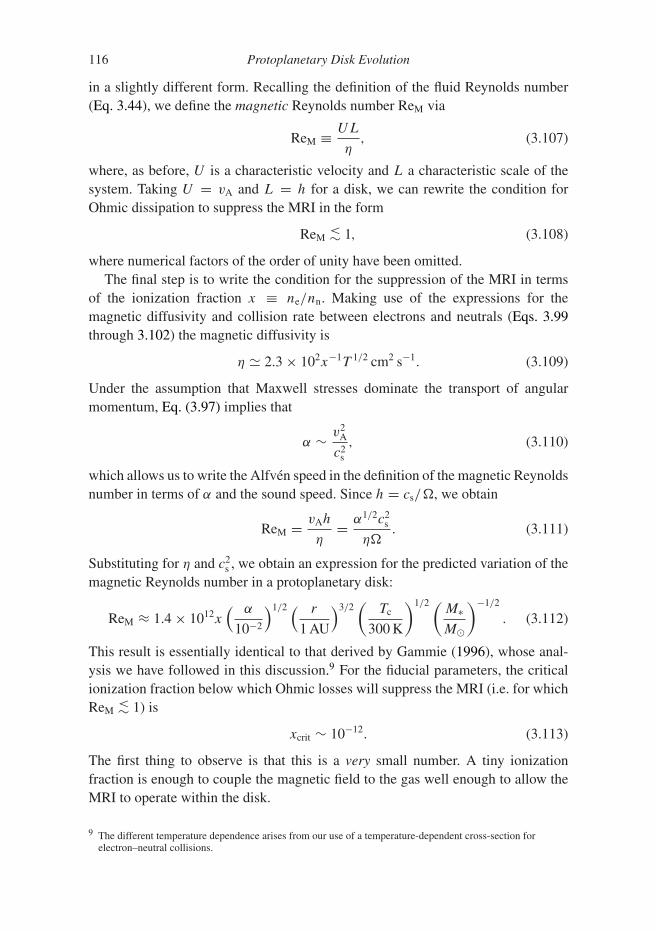
116 Protoplanetary Disk Evolution
in a slightly different form. Recalling the definition of the fluid Reynolds number(Eq. 3.44), we define the magnetic Reynolds number ReM via
ReM ≡ UL
η, (3.107)
where, as before, U is a characteristic velocity and L a characteristic scale of thesystem. Taking U = vA and L = h for a disk, we can rewrite the condition forOhmic dissipation to suppress the MRI in the form
ReM<∼ 1, (3.108)
where numerical factors of the order of unity have been omitted.The final step is to write the condition for the suppression of the MRI in terms
of the ionization fraction x ≡ ne/nn. Making use of the expressions for themagnetic diffusivity and collision rate between electrons and neutrals (Eqs. 3.99through 3.102) the magnetic diffusivity is
η � 2.3 × 10²x−1T 1/2 cm2 s−1. (3.109)
Under the assumption that Maxwell stresses dominate the transport of angularmomentum, Eq. (3.97) implies that
α ∼ v2A
c2s
, (3.110)
which allows us to write the Alfven speed in the definition of the magnetic Reynoldsnumber in terms of α and the sound speed. Since h = cs/�, we obtain
ReM = vAh
η= α1/2c2
s
η�. (3.111)
Substituting for η and c2s , we obtain an expression for the predicted variation of the
magnetic Reynolds number in a protoplanetary disk:
ReM ≈ 1.4 × 10¹²x( α
10−2
)1/2 ( r
1 AU
)3/2(
Tc
300 K
)1/2 (M∗M�
)−1/2
. (3.112)
This result is essentially identical to that derived by Gammie (1996), whose anal-ysis we have followed in this discussion.9 For the fiducial parameters, the criticalionization fraction below which Ohmic losses will suppress the MRI (i.e. for whichReM
<∼ 1) is
xcrit ∼ 10−12. (3.113)
The first thing to observe is that this is a very small number. A tiny ionizationfraction is enough to couple the magnetic field to the gas well enough to allow theMRI to operate within the disk.
9 The different temperature dependence arises from our use of a temperature-dependent cross-section forelectron–neutral collisions.

3.6 Effects of Partial Ionization and Dead Zones 117
Although xcrit is very small, it is far from obvious that even this level of ionizationis attained throughout the disk. In Section 2.8 we found that thermal ionizationof the alkali metals would yield x > xcrit for Tc
>∼ 103 K, but temperatures thishigh are only attained in the very inner disk. At larger distances from the star, theupper and lower surfaces of the disk will be well-enough ionized due to nonthermalprocesses (irradiation by the stellar X-ray flux, and/or cosmic rays) but the interiorof the disk – shielded by the high column density from these external ionizingagents – may well have x < xcrit. We conclude that close to the mid-plane theMRI at the radii of greatest interest for planet formation may be suppressed by thelow ionization fraction. A region in the disk where MHD turbulence is suppresseddue to the damping effects of non-ideal terms is described as a dead zone. If Ohmicdiffusion were really the only effect that mattered, the dead zone would stretch froman inner radius defined by thermal ionization of the alkali metals out to a distanceof the order of 10 AU.
3.6.2 Non-ideal MHD Terms
Early studies of the effect that the low ionization levels in protoplanetary disks haveon magnetic field evolution focused on the role of Ohmic diffusion. Ohmic diffusionis physically simple because it acts unconditionally to damp the MRI, but it isonly one manifestation – and normally not even the most important one – of howweakly ionized gases interact with magnetic fields. The full set of “non-ideal terms”comprises Ohmic diffusion, the Hall effect, and ambipolar diffusion. The relativeimportance of these terms varies depending on how the dynamics of charge carriersis affected by magnetic fields and by collisions with neutral species. Imagine thatwe have a mostly neutral fluid, with a small sprinkling of charge carriers in the formof electrons and ions (dust particles can also be an important charge carrier, but wewill ignore that possibility throughout). If we apply an external electric field E inthe neutral frame, the charge carriers will start accelerating. Their drift velocity –and hence the amount of electric current they generate – can be limited either bycollisions with neutrals or by magnetic forces. Three regimes can be distinguished:
• At high densities both electron and ion drift speeds are limited by collisions withneutral particles, irrespective of the magnetic field. This is the Ohmic regime.
• At intermediate densities the electron dynamics is controlled by magnetic forces,but the ions are unaffected by the field. This is the Hall regime.
• At low densities both electrons and ions are tied to the magnetic field, and bothspecies drift together relative to the neutral fluid. This is the ambipolar diffusionregime.
Despite the similar-sounding physics underlying Ohmic, Hall, and ambipolarMHD, the mathematical description and consequences of the three effects arequite distinct. We will begin by deriving the non-ideal equivalent of the induction

118 Protoplanetary Disk Evolution
equation, and then use that to estimate the physical conditions under which eachterm is dominant within disks.
3.6.3 Non-ideal Induction Equation
The physics of how magnetic fields affect weakly ionized fluids is easy to visualize.Magnetic fields exert Lorentz forces on the charged species, here supposed to beelectrons and ions, but not on the neutrals. Collisions between the neutrals andeither the ions or the electrons lead to momentum exchange whenever the neutralfluid has a velocity differential with respect to the charged fluids. The strategy fordescribing this situation is to first write down coupled momentum equations forthe three species, which together with Maxwell’s equations for the electric andmagnetic fields fully describe the evolution. Then, in the spirit of ideal MHD, weidentify approximations that allow us to reduce the system to a single momentumequation for the bulk fluid plus an evolution equation for the time dependence ofthe magnetic field.
We begin by considering the momentum equation. For the neutrals we have
ρ∂v∂t
+ ρ(v · ∇)v = −∇P − ρ∇� − pnI − pne. (3.114)
Here ρ,v, and P (without subscripts) refer to the neutral fluid, and pnI and pne
are the rate of momentum exchange due to collisions between the neutrals and theions/electrons respectively. Identical equations apply to the charged species, but forthe addition of Lorentz forces,
ρe
∂ve
∂t+ ρe(ve · ∇)ve = −∇Pe − ρe∇�
− ene
(E + ve × B
c
)− pen,
ρI
∂vI
∂t+ ρI (vI · ∇)vI = −∇PI − ρI∇�
+ ZenI
(E + vI × B
c
)− pIn. (3.115)
In these equations E and B are the electric and magnetic fields, the ionshave charge Ze, where −e is the charge on an electron, and of coursepne = −pen and pnI = −pIn. Having three momentum equations looks com-plicated, but we can make a large simplification to the system by noting that thetime scale for macroscopic evolution of the fluid is generally much longer than thetime scale for collisional or magnetic forces to alter a charged particle’s momentum.We can then ignore everything in the charged species’ momentum equations, exceptfor the Lorentz and collisional terms. For the ions we have,
ZenI
(E + vI × B
c
)− pIn = 0, (3.116)
3.6 Effects of Partial Ionization and Dead Zones 119
with a similar equation for the electrons. Imposing charge neutrality, ne = ZnI ,we eliminate the electric field between the ion and electron equations to find anexpression for the sum of the momentum transfer terms,
pIn + pen = ene
c(vI − ve) × B. (3.117)
The current density
J = ene(vI − ve), (3.118)
so we can write this as,
pIn + pen = J × Bc
. (3.119)
Finally we go to Maxwell’s equations, two of which read
∇ × E = −1
c
∂B∂t
, (3.120)
4π
cJ = ∇ × B + 1
c
∂E∂t
. (3.121)
The final term on the right-hand-side of the second equation is the displacementcurrent. Ignoring this term is the key approximation that leads to both ideal andnon-ideal MHD. To justify dropping the displacement current, consider some fluidmotion that has a characteristic length scale L and characteristic time scale T .Dimensional analysis gives the ratio of the two terms on the right-hand-side ofthe equation above as
|(1/c)∂E/∂t ||∇ × B| ∼ |BL/(c2T 2)|
|B/L| ∼ L2
c2T 2. (3.122)
Since the characteristic velocity v ∼ L/T the displacement current is of the orderof O(v2/c2) and consistently ignorable in nonrelativistic MHD flows.10 Doing so,we substitute Eq. (3.119) in the neutral equation of motion to obtain
ρ∂v∂t
+ ρ(v · ∇)v = −∇P − ρ∇� + 1
4π(∇ × B) × B. (3.123)
This is identical to the ideal MHD momentum equation that holds for a fully ionizedplasma. The triplet of momentum equations have reduced consistently to a singleequation that looks like the momentum equation for a neutral fluid, but for theaddition of a magnetic force term whose form does not depend upon the makeupof the gas.
Deducing the induction equation for non-ideal MHD amounts to finding a gener-alized version of Ohm’s law that relates the current density J to the electric field E.
10 MHD actually works perfectly well also in relativistic situations, but we have no cause to discuss the extrasubtleties involved in demonstrating this given the extremely low velocities involved in protoplanetary diskapplications.
120 Protoplanetary Disk Evolution
Once this is done the time evolution of the magnetic field follows immediately fromFaraday’s law as expressed in the Maxwell equation ∇ × E = −(1/c)∂B/∂t . Tofind Ohm’s law, we first need to define the momentum coupling terms entering intoEq. (3.115), and then make controlled approximations that allow us to drop severalof the resulting terms. The argument is somewhat delicate, but rests ultimately onthe physical fact that neutral–ion and neutral–election interactions are not identical.The derivation below is based closely on that given by Balbus (2011).
The first step is to define the momentum exchange terms. The neutral–ion andneutral–electron momentum exchange rates are written as
pnI = nμnIνnI (v − vI ),
pne = nμneνne(v − ve),(3.124)
with n being the number density of neutral particles. The reduced masses of theinteracting species are given in terms of the particle masses,
μnI = mnmI
mn + mI
, (3.125)
μne = mnme
mn + me
� me, (3.126)
where the final simplification follows because the electron mass is much smallerthan the mass of a neutral particle. The collision frequencies (denoted by ν) dependupon the cross-section σ for collisions and on the relative velocity w for collisions,
νnI = nI 〈σnIwnI 〉,νne = ne〈σnewne〉,νIn = n〈σnIwnI 〉,νen = n〈σnewne〉.
(3.127)
The angle brackets denote averages over the velocity distributions of the interact-ing species, which can be assumed to be Maxwellian. We have written all fourpermutations of the collision frequency to emphasize that, for example, νne �= νen.The former quantity is proportional to the electron number density while the latterscales with the neutral number density. The order of subscripts for most of the otherquantities is irrelevant (i.e. σnI = σIn,wnI = wIn,μnI = μIn etc.), while as notedalready pnI = −pIn.
There is not yet any physics in the above definitions. For what comes later,however, the key point is that electron–neutral collisions have significant differ-ences from ion–neutral collisions. There are two separate issues. First, in thermalequilibrium at temperature T the relative velocity of collisions scales as w ∝T 1/2μ−1/2. Electron–neutral collisions thus occur at higher w than ion–neutral col-lisions. Second, because electrons are point particles, the cross-section that entersinto their collision term with neutrals is a geometric cross-section for the neu-tral species involved. Ion–neutral collisions, on the other hand, have a long-range

3.6 Effects of Partial Ionization and Dead Zones 121
contribution and a cross-section that exceeds the geometric one. A calculation byDraine et al. (1983) gives
〈σInwIn〉 = 1.9 × 10⁻⁹ cm3 s−1,
〈σenwen〉 = 10−15
(128kBT
9πme
)1/2
cm2.(3.128)
The distinction between the two types of collisions is evidenced by the fact thatthe electron–neutral expression has the expected temperature dependence, whilethe ion–neutral expression is independent of temperature. The quantity that willinterest us is
μIn
me
〈σInwIn〉〈σenwen〉 ≈ 4.2 × 10³
(μIn
mp
)T −1/2, (3.129)
where we have written the ion–neutral reduced mass in units of the proton mass.This quantity is securely much larger than unity for all temperatures and ion massesof interest. When it crops up, we can safely neglect the denominator in favor of thenumerator.
With these preliminaries in hand we can proceed to derive a generalized Ohm’slaw. The starting point is the momentum equation for the electrons, which is exactlyanalogous to Eq. (3.116). It reads,
−ene
(E + ve × B
c
)− pen = 0. (3.130)
Recall that the key assumption that allowed us to write the momentum equationin this form was that the time scales for microscopic processes (magnetic andcollisional forces) to change the electron momentum are short compared to bulkfluid time scales. Substituting for pen = nemeνen(ve − v) yields
E + ve × Bc
+ meνen
e(ve − v) = 0. (3.131)
We seek to rewrite the second and third terms in the form of an “inductive” piece(proportional to v×B, with v the bulk fluid velocity) plus other terms that representcurrent densities. To that end, we first express Eq. (3.131) in the equivalent butlengthier form,
E + 1
c
⎡⎣v + (ve − vI )︸ ︷︷ ︸
A
+ (vI − v)︸ ︷︷ ︸B
⎤⎦
× B + meνen
e
⎡⎣(ve − vI )︸ ︷︷ ︸
A
+ (vI − v)︸ ︷︷ ︸C
⎤⎦ = 0. (3.132)

122 Protoplanetary Disk Evolution
Making use of Eq. (3.118), the relative velocity between the electron and ionfluids is
(ve − vI ) = − Jene
. (3.133)
The two terms labeled “A” in the above equation can therefore be immediatelywritten in terms of the current density J.
Term “B” and term “C” both involve (vI − v) which is proportional to pIn.To write this velocity difference as a current, we go back to Eq. (3.119),
pIn + pen = J × Bc
, (3.134)
and write out the terms on the left-hand-side explicitly,
nIμInn〈σInwIn〉(vI − v) + nemen〈σenwen〉 [(ve − vI ) + (vI − v)] . (3.135)
Using Eq. (3.129), together with the fact that the ratio ne/nI = Z is not very large,we find that the second term involving (vI − v) can be dropped. We then have
nIμInn〈σInwIn〉(vI − v) = J × Bc
+ nemen〈σenwen〉(vI − ve), (3.136)
from which it follows that
(vI − v) = 1
nIμInn〈σInwIn〉J × B
c+ ne
nI
me
μIn
〈σenwen〉〈σInwIn〉(vI − ve). (3.137)
We are now ready to substitute this expression into Eq. (3.132) but before doingso, we observe that the term involving (vI − ve) will always be smaller than thetwo terms labeled “A” (by the identical argument given above). Keeping only thefirst term on the right-hand-side gives a version of Ohm’s law that reads
E + v × Bc
− J × Benec
[1 − neme
nIμIn
〈σnewne〉〈σInwIn〉
]
+ 1
nIμInn〈σInwIn〉(J × B) × B
c2− meνen
e2ne
J = 0. (3.138)
For one last time we note that the second term in the square brackets is ignorable.Dropping that, we obtain the final form of the non-ideal Ohm’s law. To write it in itsstandard form, we introduce some additional definitions. The conductivity σ (notto be confused with the collision cross-section, for which we have used the samesymbol) is
σ = e2ne
meνen
, (3.139)
while the magnetic resistivity η is
η = c2
4πσ. (3.140)
3.6 Effects of Partial Ionization and Dead Zones 123
Finally, we have to contend with the fact that the ion–neutral collision term fromEq. (3.124) is conventionally written in terms of mass rather than number densitiesin the astrophysical literature,
pIn = ρρIγ (vI − v). (3.141)
The quantity γ is called the drag coefficient. Comparison of the above expressionwith Eq. (3.124) shows that it can be written as
γ = 〈σnIwnI 〉mn + mI
. (3.142)
An advantage of writing the collision term in this form is that γ is approximatelyconstant (Eq. 3.128).
Putting the various definitions together, the generalized form of Ohm’s law is
E + v × Bc
− Jσ
− J × Benec
+ (J × B) × Bγ c2ρρI
= 0. (3.143)
Using ∂B/∂t = −c∇ × E and J = (c/4π)∇ × B we obtain the non-ideal MHDinduction equation,
∂B∂t
= ∇ ×
⎡⎢⎢⎢⎣v × B︸ ︷︷ ︸
induction
− η∇ × B︸ ︷︷ ︸Ohmic
− J × Bene︸ ︷︷ ︸Hall
+ (J × B) × Bγ cρρI︸ ︷︷ ︸ambipolar
⎤⎥⎥⎥⎦ . (3.144)
The three different non-ideal MHD effects – Ohmic diffusion, ambipolar diffusion,and the Hall effect – are labeled, though with the derivation we have given thecorrespondence of the mathematical terms to the different regimes of fluid–magnetic field coupling is not very transparent.
3.6.4 Density and Temperature Dependence of Non-ideal Terms
The induction equation for non-ideal MHD that we have derived,
∂B∂t
= ∇ ×[
v × B − η∇ × B − J × Bene
+ (J × B) × Bγ cρρI
], (3.145)
describes the behavior of weakly-ionized magnetized fluids under conditions appro-priate to protoplanetary disks. As may be surmised from the complexity of theequation, not all of that behavior is simple or intuitive. Nonetheless a few simpleproperties stand out. The strength of the Ohmic term scales with η ∝ n−1
e , as doesthe Hall term, while ambipolar diffusion is proportional to ρ−1
I . The importance ofnon-ideal effects relative to the inductive term therefore scales with the ionizationdegree in the same way for each term. The magnetic field dependence, on the otherhand, is quite different. Noting that J ∝ ∇ × B we see that the Ohmic, Hall, andambipolar terms involve successively higher powers of B = |B|. Moreover, all of
124 Protoplanetary Disk Evolution
the terms in the equation apart from the Hall term are indifferent to the sign ofthe magnetic field, in the sense that making the substitution B → −B leaves theequation as a whole unchanged. This is not true in circumstances where the Hallterm matters, and indeed qualitatively different behavior occurs in Hall-dominatedMHD depending on the sign of large-scale magnetic fields.
The common scaling of the three non-ideal effects with ionization degree meansthat it is possible to estimate their relative importance without needing to know justhow weakly ionized the fluid is. To do so we replace the vectors in Eq. (3.145)with scalars, and replace ∇ ×B with the dimensionally equivalent B/L, where L issome characteristic length scale. For example, the ratio of the estimated magnitudesof the Ohmic and Hall terms, which we will denote by O/H, is,
O
H∼ ηB/L
B2/(Lene)∼ ηeneB
−1. (3.146)
On substituting for η from Eqs. (3.127), (3.128), and (3.140) we find that O/H ∝nT 1/2B−1, and hence in general we need to specify the density, temperature, andmagnetic field strength in order to estimate the relative importance of these twoterms. A convenient parameterization is to express the magnetic field strength indimensionless form via the ratio of the Alfven speed vA =
√B2/4πρ to the sound
speed cs . Doing so we find
O
H=
(n
8 × 1017 cm−3
)1/2 (vA
cs
)−1
, (3.147)
A
H=
(n
9 × 1011 cm−3
)−1/2 (T
100 K
)1/2 (vA
cs
), (3.148)
A
O=
(n
3 × 1015 cm−3
)−1 (T
103 K
)1/2 (vA
cs
)2
. (3.149)
These expressions allow us to calculate planes in the three-dimensional space ofdensity, temperature, and field strength, defined for example by O/H = 1, onwhich any two of the non-ideal terms have nominally equal strength. Figure 3.7shows a two-dimensional slice through this space, obtained by fixing the ratio(vA/cs) = 0.1. As expected based on both the physical origin and mathematicalrepresentation of the non-ideal terms, Ohmic diffusion dominates at high densi-ties and ambipolar diffusion at low densities. The Hall effect is expected to bemost important across several orders of magnitudes of intermediate density condi-tions. Increased temperatures favor a greater role for ambipolar diffusion over theHall term.
3.6.5 Application to Protoplanetary Disks
Given a disk model and some assumed or calculated magnetic field structure wecan use the preceding analysis to predict where in protoplanetary disks each of

3.6 Effects of Partial Ionization and Dead Zones 125
Ohmicdominated
Ambipolardominated Hall dominated
Ohmic >ambipolar
Ambipolar >Ohmic
Thermal ionization / ideal MHD
( )
( )
Figure 3.7 Approximate delineation of where the different non-ideal termsdominate in the plane of number density n and temperature T , assuming thatthe ratio of the Alfven to sound speed (vA/cs) = 0.1. Above about 103 K theionization fraction in protoplanetary disks is usually high enough that ideal MHDis a reasonable approximation.
FUV ionization
X-ray ionization
0.1 AU 1 AU 10 AU
T ~ 103 K
Ideal MHD
Ambipolar MHDin atmosphere Ambipolar MHD
in mid-plane
Hall / Ohmic mid-plane
Figure 3.8 Illustration of where different non-ideal MHD effects are expected tobe important in protoplanetary disks.
the different non-ideal terms ought to matter for the dynamics. This is an inexactscience. Besides any uncertainties in the disk model, the calculation of the O/Hand A/H ratios is crude and ignores the fact that the non-ideal terms have differingmathematical structures. Generically, however, density is the most important vari-able and we will end up with a picture something like Fig. 3.8. Three main regionscan be identified:

126 Protoplanetary Disk Evolution
• A hot thermally ionized disk region close to the star, within which ideal MHD isa reasonable approximation.
• An inner disk region, extending from the radius where the mid-plane temperatureis around 103 K out to at least several AU, where the mid-plane dynamics is con-trolled by the Hall (and possibly Ohmic) term. In the lower density atmosphereambipolar diffusion is important.
• An outer disk region where the mid-plane density is low enough that ambipolardiffusion dominates even in the mid-plane. Far ultraviolet ionization of a thinsurface layer may modify the atmosphere dynamics.
Determining the importance of these different regions for the structure and evo-lution of protoplanetary disks, and for planet formation more generally, requiresstudy of the linear properties of Eq. (3.145) together with numerical simulations ofthe nonlinear evolution of the modified MRI. In summarizing the results of suchinvestigations it is useful to rewrite the induction equation in a different form:
∂B∂t
= ∇ ×[
v × B − ηO∇ × B − ηHJ × B
B+ ηA
(J × B) × BB2
]. (3.150)
Written in this form ηO,ηH and ηA all have the dimensions of a diffusivity, althoughonly the Ohmic term truly behaves as a simple diffusion process. From the diffu-sivities we can construct two dimensionless quantities known as Elsasser numbers:
�O = v2A
�ηO(Ohmic Elsasser number), (3.151)
Am = v2A
�ηA(ambipolar Elsasser number). (3.152)
Numerical simulations show that the properties of the MRI are substantially modi-fied whenever the Ohmic or ambipolar Elsasser numbers drop below a critical value,which depends upon field geometry but is of the order of 1–10 (Turner et al., 2007;Bai & Stone, 2011). Consistent with the original dead zone concept, we thereforeexpect changes to MHD turbulence both in the mid-plane around 1 AU (whereOhmic diffusion is the dominant dissipative process) and in the disk atmosphereand at large radii of the order of 100 AU (where ambipolar diffusion dominates).In particular, turbulence in the outer regions of the disk due to MHD processes islikely to be damped by the effects of ambipolar diffusion, particularly if there islittle or no net magnetic field threading the disk (Simon et al., 2013).
A Hall Elsasser number can be defined in an analogous fashion, but this parame-terization is less useful because the Hall effect – unlike either the Ohmic or ambipo-lar terms – is nondissipative and poorly characterized as a diffusive process. TheHall term more closely resembles the inductive term ∇ × (v × B), and its strengthcan alternatively be characterized by the ratio of the Hall to the inductive term. Inthe linear regime the Hall term gives rise to a Hall shear instability (Kunz, 2008)
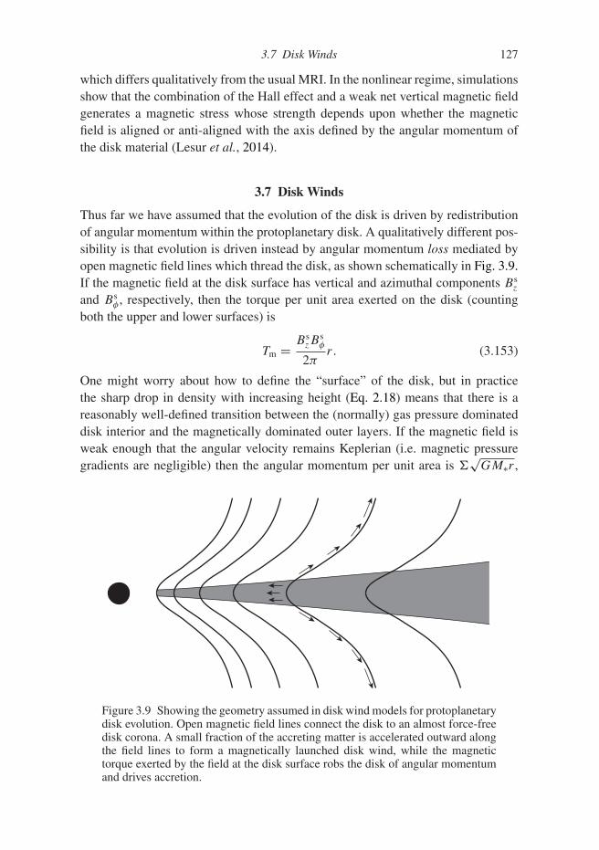
3.7 Disk Winds 127
which differs qualitatively from the usual MRI. In the nonlinear regime, simulationsshow that the combination of the Hall effect and a weak net vertical magnetic fieldgenerates a magnetic stress whose strength depends upon whether the magneticfield is aligned or anti-aligned with the axis defined by the angular momentum ofthe disk material (Lesur et al., 2014).
3.7 Disk Winds
Thus far we have assumed that the evolution of the disk is driven by redistributionof angular momentum within the protoplanetary disk. A qualitatively different pos-sibility is that evolution is driven instead by angular momentum loss mediated byopen magnetic field lines which thread the disk, as shown schematically in Fig. 3.9.If the magnetic field at the disk surface has vertical and azimuthal components Bs
z
and Bsφ , respectively, then the torque per unit area exerted on the disk (counting
both the upper and lower surfaces) is
Tm = BszB
sφ
2πr . (3.153)
One might worry about how to define the “surface” of the disk, but in practicethe sharp drop in density with increasing height (Eq. 2.18) means that there is areasonably well-defined transition between the (normally) gas pressure dominateddisk interior and the magnetically dominated outer layers. If the magnetic field isweak enough that the angular velocity remains Keplerian (i.e. magnetic pressuregradients are negligible) then the angular momentum per unit area is �
√GM∗r ,
Figure 3.9 Showing the geometry assumed in disk wind models for protoplanetarydisk evolution. Open magnetic field lines connect the disk to an almost force-freedisk corona. A small fraction of the accreting matter is accelerated outward alongthe field lines to form a magnetically launched disk wind, while the magnetictorque exerted by the field at the disk surface robs the disk of angular momentumand drives accretion.
128 Protoplanetary Disk Evolution
and the loss of that angular momentum via the magnetic torque results in a radialvelocity
|vr,m| = BszB
sφ
π��. (3.154)
This inflow velocity can be compared to that which results from internal redistribu-tion of angular momentum due to viscosity,
vr,visc = −3
2
ν
r. (3.155)
Making use of Eqs. (3.46) and (3.97), and noting that for MRI-generated transportthe Maxwell stress is dominant over the Reynolds stress,
|vr,m||vr,visc| ∼ Bs
zBsφ
BrBφ
(h
r
)−1
, (3.156)
where the magnetic fields in the denominator are the turbulent fields evaluatednear the mid-plane and we have ignored numerical factors of the order of unity.One obtains the result that if organized large-scale fields thread the disk and havecomparable strengths to the turbulent fields, a wind can carry away angular momen-tum more efficiently than internal processes can redistribute it, especially if thedisk is thin.
3.7.1 Condition for Magnetic Wind Launching
A simple model of a magnetohydrodynamic disk wind that can be analyzed quan-titatively is the Blandford–Payne wind (Blandford & Payne, 1982). The geometryof the wind is illustrated in Fig. 3.10. We envisage a Keplerian disk that is threadedby a large-scale poloidal magnetic field, and assume that there is enough ionizationfor ideal MHD to apply. Within the disk the energy density in the magnetic field,B2/8π , is smaller than ρc2
s , the thermal energy. Due to flux conservation, however,the energy in the vertical field component, B2
z /8π , is roughly constant with heightfor z < r , while the gas pressure typically decreases at least exponentially with ascale height h r . This leads to a region above the disk surface where magneticforces dominate. The magnetic force per unit volume can be written as the sum ofa magnetic pressure gradient and a force due to magnetic tension,
J × Bc
= −∇(
B2
8π
)+ B · ∇B
4π, (3.157)
where the current
J = c
4π∇ × B. (3.158)

3.7 Disk Winds 129
B2 / 8p < P
B2 / 8p >> P, rv2
B2 / 8 < rv2
Force-freeregion
B
Alfvénsurface
Ω
l = Ω0r02
l = Ω0rA2
p
Figure 3.10 Illustration of the different physical regions of a Blandford–Paynedisk wind (Spruit, 1996). We determine the condition for magnetic launching of awind by noting that the magnetic field in the force-free region behaves as a rigidwire. Gas tied to the field lines behaves mechanically as if it is a bead strung to thewire, and can escape the disk if the centrifugal force exceeds that of gravity.
In the disk wind region where magnetic forces dominate, the requirement that theyexert a finite acceleration on the low density gas can only be satisfied if the forceapproximately vanishes, i.e. that
J × B ≈ 0. (3.159)
The structure of the magnetic field in the magnetically dominated region is thendescribed as being “force-free,” and in the disk wind case (where B changes slowlywith z) the field lines must be approximately straight to ensure that the magnetictension term is small. If the field lines support a wind, the force-free structurepersists up to where the kinetic energy density in the wind, ρv2, first exceedsthe magnetic energy density. This criterion defines the Alfven surface. Beyond theAlfven surface, the inertia of the gas in the wind is sufficient to bend the field lines,which wrap up into a spiral structure as the disk below them rotates.
Magneto-centrifugal driving can launch a wind from the surface of a cold gasdisk if the magnetic field lines are sufficiently inclined to the disk normal. Thecritical inclination angle in ideal MHD can be derived via a mechanical analogy(which is in fact exact). To proceed, we note that in the force-free region themagnetic field lines are (i) basically straight lines, and (ii) enforce rigid rotationout to the Alfven surface at an angular velocity equal to that of the disk at the field
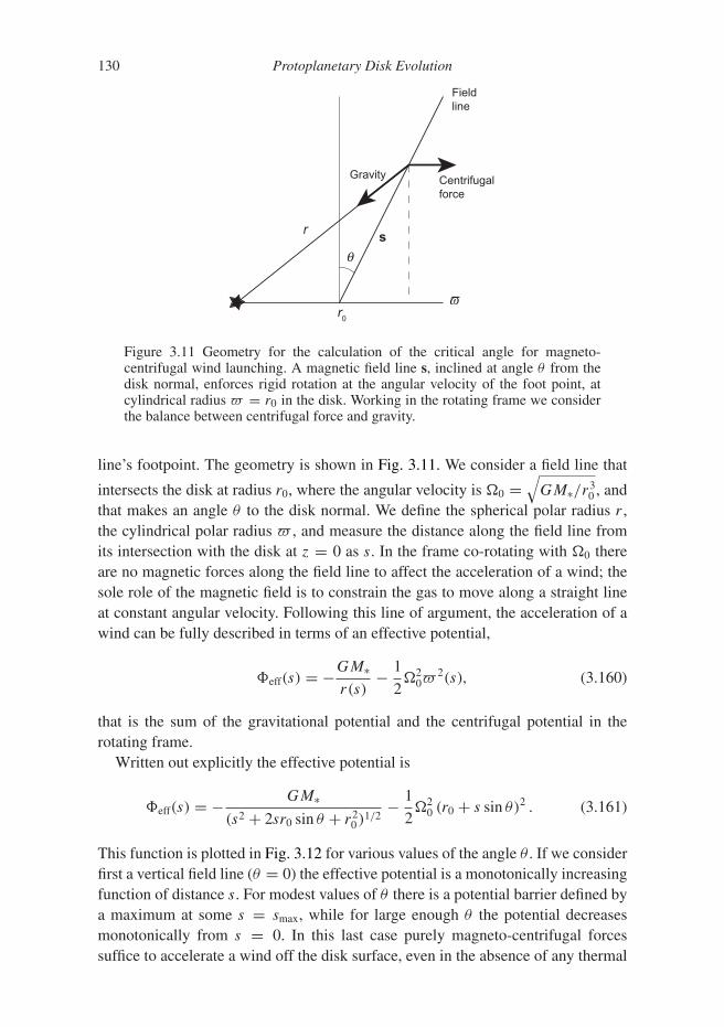
130 Protoplanetary Disk Evolution
r0
sq
v
r
Centrifugalforce
Gravity
Fieldline
Figure 3.11 Geometry for the calculation of the critical angle for magneto-centrifugal wind launching. A magnetic field line s, inclined at angle θ from thedisk normal, enforces rigid rotation at the angular velocity of the foot point, atcylindrical radius � = r0 in the disk. Working in the rotating frame we considerthe balance between centrifugal force and gravity.
line’s footpoint. The geometry is shown in Fig. 3.11. We consider a field line that
intersects the disk at radius r0, where the angular velocity is �0 =√
GM∗/r30 , and
that makes an angle θ to the disk normal. We define the spherical polar radius r ,the cylindrical polar radius � , and measure the distance along the field line fromits intersection with the disk at z = 0 as s. In the frame co-rotating with �0 thereare no magnetic forces along the field line to affect the acceleration of a wind; thesole role of the magnetic field is to constrain the gas to move along a straight lineat constant angular velocity. Following this line of argument, the acceleration of awind can be fully described in terms of an effective potential,
�eff(s) = −GM∗r(s)
− 1
2�2
0�2(s), (3.160)
that is the sum of the gravitational potential and the centrifugal potential in therotating frame.
Written out explicitly the effective potential is
�eff(s) = − GM∗(s2 + 2sr0 sin θ + r2
0 )1/2− 1
2�2
0 (r0 + s sin θ)2 . (3.161)
This function is plotted in Fig. 3.12 for various values of the angle θ . If we considerfirst a vertical field line (θ = 0) the effective potential is a monotonically increasingfunction of distance s. For modest values of θ there is a potential barrier defined bya maximum at some s = smax, while for large enough θ the potential decreasesmonotonically from s = 0. In this last case purely magneto-centrifugal forcessuffice to accelerate a wind off the disk surface, even in the absence of any thermal

3.7 Disk Winds 131
Figure 3.12 The variation of the disk wind effective potential �eff (in arbitraryunits) with distance s along a field line. From top downwards, the curves showfield lines inclined at 0◦,10◦,20◦,30◦ (in bold) and 40◦ from the normal to thedisk surface. For angles of 30◦ and more from the vertical, there is no potentialbarrier to launching a cold MHD wind directly from the disk surface.
effects. We compute the critical inclination angle θcrit, defined as the minimumangle that allows magneto-centrifugal wind driving, via the condition
∂2�eff
∂s2
∣∣∣∣s=0
= 0. (3.162)
Evaluating this condition, we find,
1 − 4 sin2 θcrit = 0
⇒ θcrit = 30◦, (3.163)
as the minimum inclination angle from the vertical needed for unimpeded windlaunching in ideal MHD.
The rigid rotation of the field lines interior to the Alfven surface means thatgas being accelerated along them increases its specific angular momentum. Themagnetic field, in turn, applies a torque to the disk that removes a correspondingamount of angular momentum. If a field line, anchored to the disk at radius r0,crosses the Alfven surface at (cylindrical) radius rA, it follows that the angularmomentum flux is
Lw = Mw�0r2A, (3.164)
where Mw is the mass loss rate in the wind. Removing angular momentum at thisrate from the disk results in a local accretion rate M = 2Lw/�0r
20 . The ratio of the
disk accretion rate to the wind loss rate is
M
Mw= 2
(rA
r0
)2
. (3.165)
132 Protoplanetary Disk Evolution
If rA substantially exceeds r0 (by a factor of a few, which is reasonable for detaileddisk wind solutions) a relatively weak wind can carry away enough angular momen-tum to support a much larger accretion rate.
3.7.2 Net Flux Evolution
It is straightforward to generalize the surface density evolution Eq. (3.6) to includethe effect of angular momentum loss in a disk wind. If the angular velocity remainsKeplerian the effect of the wind on the disk can be modeled as an additional advec-tive term,
∂�
∂t= 3
r
∂
∂r
[r1/2 ∂
∂r
(ν�r1/2
)] − 1
r
∂
∂r
(r�vr,m
). (3.166)
The potential presence of MHD disk winds has two important implications. First,winds can make a qualitative change to the predicted evolution of the outer diskradius with time. A disk in which accretion is driven solely by angular momentumredistribution expands with time, while one driven entirely by angular momentumloss in a wind shrinks. Second, including the possibility of winds breaks any linkagebetween disk evolution and disk turbulence. If the disk accretes due to angularmomentum redistribution, then knowing the time scale for disk evolution gives anidea – admittedly a rough one – on the level of turbulence, which is important formany aspects of planet formation. In contrast, a wind-driven disk could still beturbulent, but it could in principle be almost entirely laminar.
A complete model for the evolution of the protoplanetary disk under the actionof MHD disk winds requires understanding how much mass is lost from the disk ateach radius, and how the poloidal magnetic fields that support the wind themselvesevolve. Neither of these are easy problems. High energy radiation can heat thesurface layers of the disk to a point where the gas is unbound, and can escape.In isolation this process, described as photoevaporation (Section 3.8.1), is efficientenough to explain the dispersal of low-mass disks at the end of the Class II phase.If poloidal magnetic fields are present, the rate of mass loss will then be determinedby the interplay of thermal and magneto-centrifugal effects. The field evolution isalso hard to calculate robustly. Since the flux threading the disk,
� =∮
BzdS, (3.167)
is a conserved quantity, development of net vertical field cannot occur as a result oflocal dynamo processes, but rather requires that magnetic flux of one sign either bedragged into or preferentially expelled from the disk. In modern day star formation,disks form from molecular cloud cores that contain magnetic fields, and it is rea-sonable to think that young disks, at least, are threaded by some net flux. Over timethis flux can be advected inward by the accretion flow, on a time scale given by the

3.8 Disk Dispersal 133
viscous time scale τν = r2/ν (Eq. 3.12). Flux can also escape outward if there isa large enough effective magnetic diffusivity. The simplest quantitative descriptionof the competition between inward advection and outward diffusion was developedby Lubow et al. (1994). For Bs
z ∼ Bsr they found that the outward diffusion time
scale is given by
tη � r2
η
(h
r
), (3.168)
where η is the magnetic diffusivity within the disk. If the diffusivity and the vis-cosity are both generated from the same turbulent processes within the disk, weexpect that to order of magnitude η ∼ ν, and hence tη ∼ (h/r)tν . More detailedcalculations by Guilet and Ogilvie (2014) suggest that the difference between tη andtν is smaller, and that the magnetic field in the inner disk can find an equilibriumvalue of the plasma β that measures the ratio of the mid-plane thermal pressure tothe magnetic pressure. The actual value of β that results is, however, hard enough tocompute that it remains unclear (on first principles grounds) whether net magneticfields have a dominant influence on disk evolution.
3.8 Disk Dispersal
Depletion of the gaseous protoplanetary disk due to stellar accretion is predictedto be a gradual process. If we consider the self-similar solution (Eq. 3.25), forexample, we find that for a time-independent viscosity scaling with radius as ν ∝ rγ
the late-time behavior of the surface density is
� ∝ t−(5/2−γ )/(2−γ ), (3.169)
which is a power-law in time (� ∝ t−3/2 for the case of ν ∝ r). A disk that evolveddue only to accretion would steadily become optically thin over an increasing rangeof radii, in the process transitioning rather slowly from a Class II to a Class IIIsource. Observationally this is not what is observed. Although a number of candi-date transition disks are known – typically YSOs that lack a near-IR excess despitethe presence of a robust mid-IR excess – the scarcity of such systems suggests thatthe dispersal phase of protoplanetary disks lasts of the order of 105 yr (Simon &Prato, 1995; Wolk & Walter, 1996). The relative brevity of the dispersal time scalesuggests that additional physical processes beyond viscous evolution contributeto the loss of gas from the disk. Plausibly the additional evolutionary agent isphotoevaporation, a process in which UV or X-ray radiation heats the disk surfaceto the point at which it becomes hot enough to escape the gravitational potential asa thermally driven wind. Photoevaporative flows from young stars with disks areobserved in the Orion nebula cluster (O’Dell et al., 1993; Johnstone et al., 1998),where an intense ionizing radiation field is provided by massive stars. Weaker UV

134 Protoplanetary Disk Evolution
irradiation originating from low mass stars themselves would suffice to dispersedisks more generally on time scales consistent with those inferred observationally.
3.8.1 Photoevaporation
The basic physics of photoevaporation is simple: UV or X-ray radiation heats thedisk surface to a temperature high enough that the thermal energy of the gas exceedsits gravitational binding energy. A pressure gradient drives this unbound gas awayfrom the star, dispersing the disk. The details of photoevaporation depend upon thesource of the irradiating flux (which can be the disk-bearing star itself or exter-nal stars in a cluster) and the energy of the photons. Extreme ultraviolet (EUV)radiation (E > 13.6 eV,λ < 912 A) ionizes hydrogen atoms, producing a sharplydefined layer of hot gas whose temperature, around 104 K, is almost independentof the density of the disk at the radius under consideration. Far ultraviolet radiation(6 eV < E < 13.6 eV) dissociates H2 molecules, creating a neutral atomic layerwhose temperature depends upon the precise balance of heating and cooling pro-cesses. Typical values are 100–5000 K. X-rays likewise produce a surface region ofheated gas with a complex vertical structure.
Complete models of photoevaporative flows need at a minimum to include thesource (either the central star or external stars) of high-energy radiation, and itscomplete spectrum. We can gain some insight by considering a simple model ofphotoevaporation due to EUV irradiation by the central star, which is easier to study(both analytically and numerically) than the general case.
Let us consider a disk exposed to EUV flux from the central star, as shown inFig. 3.13. The photoionized gas has a temperature T � 104 K, which correspondsto a sound speed cs � 10 km s−1. We define the gravitational radius rg to be thelocation where the sound speed in the ionized gas equals the orbital velocity,
rg = GM∗c2
s
= 8.9
(M∗M�
)( cs
10 km s−1
)−2AU. (3.170)
In the simplest analysis, gas at r < rg is bound, and forms an extended atmosphereabove the neutral disk surface with a scale-height h ∝ r3/2. Beyond rg the ionizedgas is unbound, and escapes the disk at a rate
�wind ∼ 2ρ0(r)cs, (3.171)
where ρ0, the density at the base of the ionized layer, is determined by the inten-sity of the irradiating EUV flux. Radiative transfer calculations by Hollenbachet al. (1994) suggest that, while the inner disk is present, the flux at r > rg isdominated by photons generated from recombinations in the atmosphere at smallerradii, and that the base density scales with radius roughly as ρ0(r) ∝ r−5/2. Mostof the mass loss is then concentrated at radii near rg.
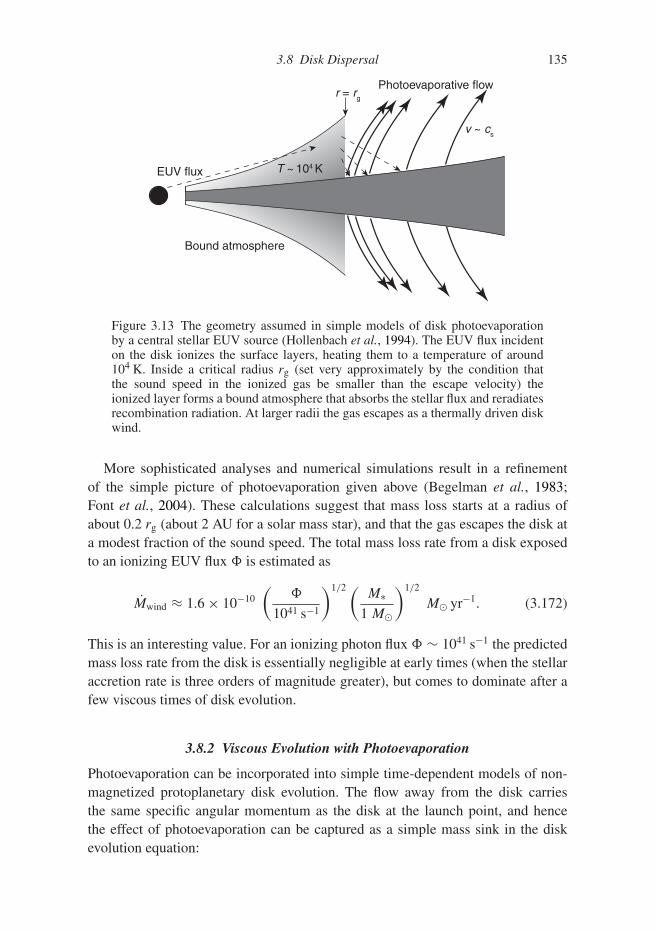
3.8 Disk Dispersal 135
Bound atmosphere
r = rg
Photoevaporative flow
EUV flux
v ~ cs
T ~ 104 K
Figure 3.13 The geometry assumed in simple models of disk photoevaporationby a central stellar EUV source (Hollenbach et al., 1994). The EUV flux incidenton the disk ionizes the surface layers, heating them to a temperature of around104 K. Inside a critical radius rg (set very approximately by the condition thatthe sound speed in the ionized gas be smaller than the escape velocity) theionized layer forms a bound atmosphere that absorbs the stellar flux and reradiatesrecombination radiation. At larger radii the gas escapes as a thermally driven diskwind.
More sophisticated analyses and numerical simulations result in a refinementof the simple picture of photoevaporation given above (Begelman et al., 1983;Font et al., 2004). These calculations suggest that mass loss starts at a radius ofabout 0.2 rg (about 2 AU for a solar mass star), and that the gas escapes the disk ata modest fraction of the sound speed. The total mass loss rate from a disk exposedto an ionizing EUV flux � is estimated as
Mwind ≈ 1.6 × 10⁻¹⁰
(�
1041 s−1
)1/2 (M∗
1 M�
)1/2
M� yr−1. (3.172)
This is an interesting value. For an ionizing photon flux � ∼ 1041 s−1 the predictedmass loss rate from the disk is essentially negligible at early times (when the stellaraccretion rate is three orders of magnitude greater), but comes to dominate after afew viscous times of disk evolution.
3.8.2 Viscous Evolution with Photoevaporation
Photoevaporation can be incorporated into simple time-dependent models of non-magnetized protoplanetary disk evolution. The flow away from the disk carriesthe same specific angular momentum as the disk at the launch point, and hencethe effect of photoevaporation can be captured as a simple mass sink in the diskevolution equation:

136 Protoplanetary Disk Evolution
∂�
∂t= 3
r
∂
∂r
[r1/2 ∂
∂r
(ν�r1/2
)] + �wind(r,t). (3.173)
The mass loss term must be specified via a model of the photoevaporation process,which in turn will depend nonlocally on the disk properties and on the strength andtime evolution of the FUV, EUV, and X-ray irradiation.
Models that combine viscous disk evolution with EUV photoevaporation(Clarke et al., 2001; Alexander et al., 2006) provide a qualitative picture for howdisk dispersal may proceed. Three phases in the evolution can be distinguished.In the first phase, mass loss due to photoevaporation is negligible compared tothe mass flux flowing through the disk as a result of viscous transport of angularmomentum, and the disk evolves as if there were no mass loss. Eventually, the massaccretion rate drops to become comparable to the wind mass loss rate, and massflowing in toward the star from large disk radii is diverted into the wind rather thanreaching the inner disk. An annular gap develops in the disk near rg, and the innerdisk, now cut off from resupply, drains rapidly on to the star on its own viscous timescale of the order of 105 yr. Figures 3.14 and 3.15 show the evolution of the massaccretion rate and disk surface density up to this point. Finally, the disk interior torg becomes optically thin to the stellar EUV flux, which then directly illuminatesthe inner edge of the outer disk. This results in an increased rate of mass loss due
Figure 3.14 The numerically computed stellar accretion rate for protoplanetarydisk models with (solid line) and without (dashed line) photoevaporative massloss. The model, which is based on that in Clarke et al. (2001), assumes a viscosityν ∝ r , and photoevaporative mass loss that scales as �wind ∝ r−5/2 outside rg =5 AU. No mass loss is assumed to occur within rg. The mass loss rate integratedfrom rg to 25 AU is 10−9 M� yr−1. The initial surface density profile matchesthe self-similar solution with an initial accretion rate of 3 × 10⁻⁷ M� yr−1 and acut-off at 10 AU. The viscosity is normalized such that the viscous time scale at10 AU is 3×10⁵ yr. The presence of a wind from the outer disk results in a sharplydefined epoch of disk dispersal.
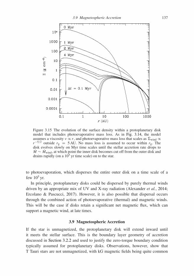
3.9 Magnetospheric Accretion 137
()
Figure 3.15 The evolution of the surface density within a protoplanetary diskmodel that includes photoevaporative mass loss. As in Fig. 3.14, the modelassumes a viscosity ν ∝ r , and photoevaporative mass loss that scales as �wind ∝r−5/2 outside rg = 5 AU. No mass loss is assumed to occur within rg. Thedisk evolves slowly on Myr time scales until the stellar accretion rate drops toM ∼ Mwind, at which point the inner disk becomes cut off from the outer disk anddrains rapidly (on a 105 yr time scale) on to the star.
to photoevaporation, which disperses the entire outer disk on a time scale of afew 105 yr.
In principle, protoplanetary disks could be dispersed by purely thermal windsdriven by an appropriate mix of UV and X-ray radiation (Alexander et al., 2014;Ercolano & Pascucci, 2017). However, it is also possible that dispersal occursthrough the combined action of photoevaporative (thermal) and magnetic winds.This will be the case if disks retain a significant net magnetic flux, which cansupport a magnetic wind, at late times.
3.9 Magnetospheric Accretion
If the star is unmagnetized, the protoplanetary disk will extend inward untilit meets the stellar surface. This is the boundary layer geometry of accretiondiscussed in Section 3.2.2 and used to justify the zero-torque boundary conditiontypically assumed for protoplanetary disks. Observations, however, show thatT Tauri stars are not unmagnetized, with kG magnetic fields being quite common
138 Protoplanetary Disk Evolution
(Johns-Krull, 2007). These fields are strong enough to disrupt the disk close to thestar, resulting in a magnetospheric accretion flow geometry in which gas at smallradii flows in along field lines to strike the star in accretion hot spots away fromthe stellar equator.11 The simplest geometry to consider is one in which the stellarmagnetic field is dipolar, aligned with the stellar rotation axis, and perpendicular tothe disk plane. The unperturbed field has a vertical component at the disk surface,
Bz = B∗
(r
R∗
)−3
, (3.174)
which falls off rapidly with increasing distance (note that B∗R3∗ = μ, the stellar
dipole moment). In the presence of a disk, the vertical field will thread the disk gasand – as long as the coupling between the magnetic field and the matter is goodenough – the field will be distorted by differential rotation between the Kepleriandisk and the star. The differential rotation will twist the field lines that couple thedisk to the star, generating an azimuthal field component at the disk surface Bφ .Computing this field accurately is not an easy matter (it may depend, for example,on the nature of the turbulence within the disk), but to an order of magnitude it isreasonable to assume that the rapid differential rotation results in a field
Bφ ∼ Bz, (3.175)
which is limited by the onset of instabilities that afflict very strongly twisted fields(Lynden-Bell & Boily, 1994). If we define the co-rotation radius rco as the radiuswhere the field lines – rotating with stellar rotation period P – have the sameangular velocity as that of Keplerian gas in the disk,
rco =(
GM∗P 2
4π2
)1/3
, (3.176)
we can identify two regions of star–disk magnetic interaction:
• Interior to co-rotation (r < rco) the disk gas has a greater angular velocity thanthe field lines. Field lines that link the disk and the star in this region are draggedforward by the disk, and exert a braking torque that tends to remove angularmomentum from the disk gas.
• Outside co-rotation (r > rco) the disk gas has a smaller angular velocity than thefield lines. The field lines are dragged backward by the disk, and the couplingresults in a positive torque on the disk gas.
Young stars are typically rapid rotators, with periods of a week or less, so the co-rotation radius that separates these two regimes lies in the inner disk. For P =7 days, for example, the co-rotation radius around a solar mass star is at rco � 15 R�or 0.07 AU.
11 This accretion geometry was initially studied for accretion on to magnetized compact objects (Pringle &Rees, 1972; Ghosh & Lamb, 1979) and subsequently applied to accretion on to T Tauri stars (Konigl, 1991).

3.9 Magnetospheric Accretion 139
The radius within which the external torque due to the star–disk magnetic inter-action dominates over the internal viscous torque is estimated by comparing thetime scales on which each mechanism removes the angular momentum of the diskgas. The stellar magnetosphere threading the disk will remove angular momentum(interior to co-rotation) on a time scale that is the angular momentum content perunit area divided by the magnetic torque (given by Eq. 3.153),
tm � 2π�
√GM∗r
BszB
sφr
, (3.177)
with the magnetic fields being evaluated at the disk surface. Equating this to theviscous time scale (tν � r2/ν) defines the magnetospheric radius
rm �(
3B2∗R
6∗
2M√
GM∗
)2/7
. (3.178)
In deriving this expression we have made use of the steady-state disk relationν� = M/(3π) and assumed the undistorted dipolar magnetic field geometry dis-cussed above. The scaling of the magnetospheric radius with the magnetic fieldstrength and mass accretion rate is robust – in fact the same scalings apply to theAlfven radius derived for spherical accretion – but equally valid physical argu-ments result in different numerical factors. Adopting the expression above, themagnetospheric radius for fiducial T Tauri parameters (B∗ = 1 kG,R∗ = 2 R�,M = 10−8 M� yr−1,M∗ = M�) is
rm � 16 R�. (3.179)
One concludes that kG-strength stellar magnetic fields are strong enough to domi-nate the dynamics of protoplanetary disks in the innermost regions, and that a stellarmagnetosphere that extends out to roughly the co-rotation radius is plausible.
The presence of magnetospheric rather than boundary layer accretion means thatprotoplanetary disks around magnetic stars are predicted to have inner edges thatlie at r � rm rather than at the stellar equator. At smaller radii there is a low densitymagnetospheric cavity within which gas is channeled on to the star along fieldlines at roughly the free-fall velocity. This geometry has a number of observationalimplications:
• The innermost region of the disk that would otherwise produce strong near-IRemission is missing. This alters the IR colors of classical T Tauri stars.
• The final accretion on to the stellar surface occurs at roughly the free-fall velocity.This explains the P Cygni profiles (indicative of infall) that are seen in somespectral lines (Hartmann et al., 1994).
• The zero-torque inner boundary condition that is justified for boundary layeraccretion need no longer apply. Instead, the star’s spin angular momentum canbe coupled to the disk angular momentum via the torque exerted by the magneticfield. This torque can modify the stellar rotation rate.

140 Protoplanetary Disk Evolution
Although important in their own right most of these effects apply at radii that aresmall enough (r <∼ 0.1 AU) to be relatively unimportant for planet formation. Thechange to the inner boundary condition formally alters the steady-state disk surfacedensity profile everywhere, but the fractional change becomes small well away fromthe inner boundary at r � rm. The presence of a low density magnetospheric cavityis of greater interest for models of planet migration (discussed in Chapter 7), whichcommonly invoke angular momentum loss to the gaseous protoplanetary disk as thedriver of orbital decay. Such migration is likely to slow and eventually halt once theplanet enters the magnetospheric cavity.
3.10 Further Reading
Accretion Power in Astrophysics, J. Frank, A. King, & D. Raine (2002), Cambridge:Cambridge University Press.
“Accretion Discs in Astrophysics,” J. E. Pringle (1981), Annual Review of Astronomy &Astrophysics, 19, 137.
“Instability, Turbulence, and Enhanced Transport in Accretion Disks,” S. A. Balbus & J. F.Hawley (1998), Reviews of Modern Physics, 70, 1.
“Dynamics of Protoplanetary Disks,” P. J. Armitage (2011), Annual Review of Astronomy& Astrophysics, 49, 195.
“Transport and Accretion in Planet-Forming Disks,” N. J. Turner, et al. (2014), in Proto-stars and Planets VI, H. Beuther, R. S. Klessen, C. P. Dullemond, and T. Henning(eds.), Tucson: University of Arizona Press, p. 411.

4
Planetesimal Formation
The formation of terrestrial planets from micrometer-sized dust particles requiresgrowth through at least 12 orders of magnitude in size scale. It is conceptuallyuseful to divide the process into three main stages that involve different dominantphysical processes:
• Planetesimal formation. Planetesimals are primordial bodies with sizes that,depending upon how they formed, may have ranged between 100 m and a fewhundred km in size. Reaching this size is doubly consequential. For an individualbody it marks a transition between bodies whose strength is determined entirelyby their material properties, and larger ones that resist disruption because ofself-gravity. For a population of bodies, the planetesimal scale matters becauseat a similar scale orbital evolution is dominated by mutual gravitational inter-actions rather than aerodynamic coupling to the gas disk. Material properties(loosely how “sticky” small particles are upon collision), aerodynamic and grav-itational physics all play a key role in solid evolution up to the formation ofplanetesimals.
• Terrestrial planet formation. Once a population of planetesimals has formedwithin the disk their dynamical evolution is dominated by gravitational interac-tions. Growth can occur from a combination of planetesimal–planetesimal (andlater protoplanet–planetesimal) collisions, and from the aerodynamically assistedaccretion of smaller solid particles that were not previously incorporated intoplanetesimals. The latter process is called “pebble accretion.”
• Giant planet formation and core migration. Once planets have grown to aboutan Earth mass, coupling to the gas disk becomes significant once again, thoughnow it is gravitational rather than aerodynamic forces that matter. For Mp ∼ M⊕this coupling can result in eccentricity damping and exchange of orbital angu-lar momentum with the gas (a process described as migration), while forMp ∼ 10 M⊕ the interaction becomes strong enough that the planet can startto capture an envelope from the protoplanetary disk.
141

142 Planetesimal Formation
The boundaries between these regimes are somewhat arbitrary and inconsistentlydefined, but it is useful to keep this ordering of the most important physics in mindas we discuss planet formation.
4.1 Aerodynamic Drag on Solid Particles
Consider a spherical particle of solid material of radius s and material density ρm.The first step to understanding how such a particle evolves within the protoplanetarydisk is to calculate the aerodynamic force experienced by the particle when it movesat a velocity v relative to the local velocity of the gas disk. In calculating the forcethere are two physical regimes to consider. If s <∼ λ, the mean-free path of gasmolecules within the disk, then the fluid on the scale of the particle is effectivelya collisionless ensemble of molecules with a Maxwellian velocity distribution. Thedrag force in this regime – which is normally the most relevant for small particleswithin protoplanetary disks – is called Epstein drag. In the alternate Stokes dragregime, which applies for s >∼ λ, the disk gas flows as a fluid around the obstructionpresented by the particle. In either regime the force scales with the frontal area πs2
that the particle presents to the gas. This means that the acceleration caused bygas drag – which is proportional to the drag force divided by the particle mass –decreases with particle size (as s−1 for spherical particles) and eventually becomesnegligible once bodies of planetesimal size have formed.
4.1.1 Epstein Drag
Epstein drag is felt by solid particles that are smaller than the mean-free path of gasmolecules within the disk. The form of the drag law in this regime can be derivedby considering the frequency of collisions between the particle and gas molecules,given by elementary arguments as the product of the collision cross-section, relativevelocity, and molecule number density. We model the solid particle as a sphere ofradius s moving with velocity v relative to the disk gas. Within the gas the meanthermal speed of the molecules is
vth =√
8kBT
πμmH. (4.1)
The gas temperature and density are T and ρ, and the mean molecular weight is μ.Up to factors of the order of unity, the frequency with which gas molecules collidewith the “front” side of the particle is
f+ ≈ πs2(vth + v)ρ
μmH, (4.2)
while the collision frequency on the back side is
f− ≈ πs2(vth − v)ρ
μmH. (4.3)

4.1 Aerodynamic Drag on Solid Particles 143
Noting that the momentum transfer per collision is approximately given by2μmHvth, we find that the net drag force in the Epstein regime scales as
FD ∝ −s2ρvthv. (4.4)
The force is linear in the relative velocity and proportional to the surface area ofthe particle and to the thermal speed of molecules in the disk gas. A more accuratederivation, valid for s < λ, v vth, and a Maxwellian distribution of molecularspeeds, yields
FD = −4π
3ρs2vthv. (4.5)
The drag force, of course, acts in the opposite direction to the vector describingthe relative velocity between the particle and the gas. Extensions to this formula todescribe the case where the particle moves supersonically with respect to the gas(v >∼ vth) can be found in Kwok (1975), though it is normally the subsonic regimethat is relevant for protoplanetary disks.
4.1.2 Stokes Drag
Once particles grow to a size much larger than the molecular mean-free path theinteraction with the gas can be treated in classical fluid terms, without reference tothe molecular nature of the gas. Drag in this regime is called Stokes drag. Naively,we might guess that the drag force would scale with the ram pressure experiencedby the particle, and hence we write the force as
FD = −CD
2πs2ρvv, (4.6)
where CD, the drag coefficient, describes how aerodynamic the particle is. In gen-eral, CD will depend upon the shape of the particle, but for spherical particles itdepends only upon the fluid Reynolds number (Eq. 3.44), which we define here onthe scale of the particle as
Re = 2sv
νm. (4.7)
Note that the viscosity here is the (small) molecular viscosity of the gas, ratherthan any turbulent viscosity within the disk. In terms of the Reynolds number,Weidenschilling (1997b) quotes a piecewise expression for scaling of the dragcoefficient:
CD � 24Re−1, Re < 1, (4.8)
CD � 24Re−0.6, 1 < Re < 800, (4.9)
CD � 0.44, Re > 800. (4.10)

144 Planetesimal Formation
Comparison of the expressions for Epstein and Stokes drag shows that they areequal for a particle of size s = 9λ/4, and this can be taken as the transition sizewhen constructing a smooth drag law that encompasses both regimes.
4.2 Dust Settling
Aerodynamic drag on particles is important for understanding both the verticaldistribution and radial motion of dust and larger bodies within the protoplanetarydisk. More subtle issues concern the interaction between aerodynamic forces andturbulence, which we have already noted is likely to be a ubiquitous feature (albeitwith poorly determined properties) of the disk. To begin with, we ignore turbulenceand consider the vertical settling and growth of dust particles suspended in a laminardisk. We quantify the coupling between the solid and gas components of the diskby defining the friction time scale for a particle of mass m as
tfric = mv
|FD|, (4.11)
where, as before, v is the relative velocity between the particle and the gas. Formany purposes, a dimensionless version of the friction time that is obtained bymultiplying by the local Keplerian angular velocity is more physically meaningful:
τfric ≡ tfric�K. (4.12)
The dimensionless friction time is also called the dimensionless stopping time andthe Stokes number.
The friction time scale measures the time in which drag modifies the relativevelocity significantly. Writing the particle mass m = (4/3)πs3ρm in terms of thematerial density ρm,tfric takes on a simple form in the Epstein drag regime:
tfric = ρm
ρ
s
vth. (4.13)
Adopting conditions appropriate for a particle at the mid-plane of the protoplane-tary disk at r = 1 AU (ρ = 10−9 g cm−3, ρm = 3 g cm−3,vth = 105 cm s−1) weobtain an estimate for the friction time scale for a particle of size s = 1μm:
tfric ≈ 3 s. (4.14)
Small dust particles are thus very tightly coupled to the gas.We now consider the forces acting on a small dust particle at height z above the
mid-plane of a laminar disk. Concentrating for now just on the vertical forces, thez component of the stellar gravity yields a downward force
|Fgrav| = m�2z, (4.15)
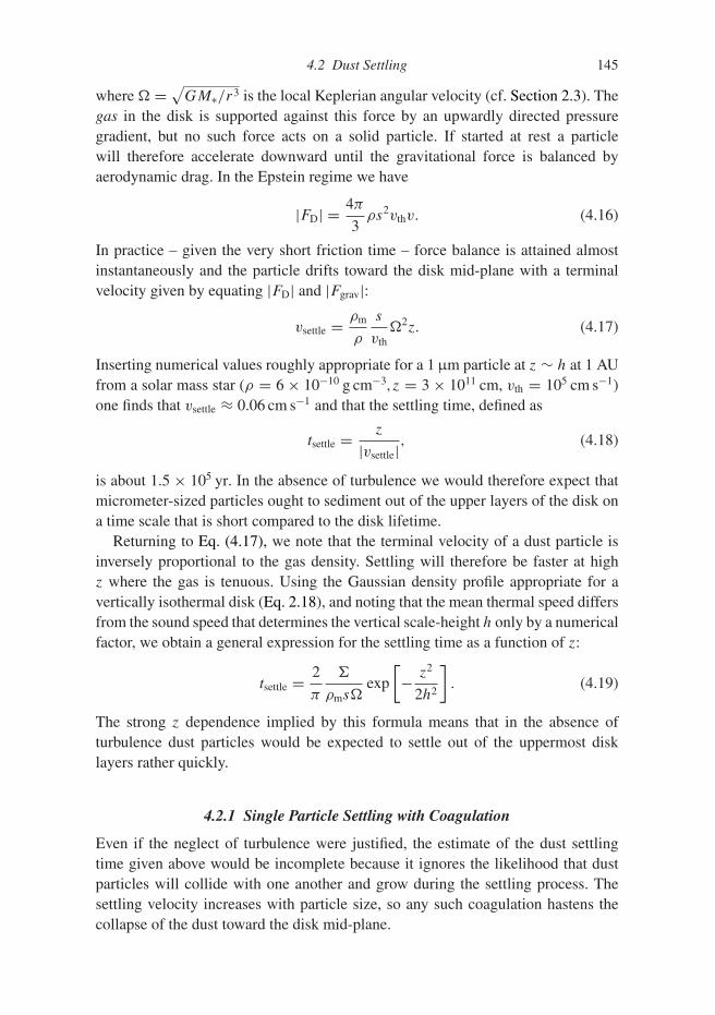
4.2 Dust Settling 145
where � =√
GM∗/r3 is the local Keplerian angular velocity (cf. Section 2.3). Thegas in the disk is supported against this force by an upwardly directed pressuregradient, but no such force acts on a solid particle. If started at rest a particlewill therefore accelerate downward until the gravitational force is balanced byaerodynamic drag. In the Epstein regime we have
|FD| = 4π
3ρs2vthv. (4.16)
In practice – given the very short friction time – force balance is attained almostinstantaneously and the particle drifts toward the disk mid-plane with a terminalvelocity given by equating |FD| and |Fgrav|:
vsettle = ρm
ρ
s
vth�2z. (4.17)
Inserting numerical values roughly appropriate for a 1μm particle at z ∼ h at 1 AUfrom a solar mass star (ρ = 6 × 10⁻¹⁰ g cm−3,z = 3 × 1011 cm, vth = 105 cm s−1)one finds that vsettle ≈ 0.06 cm s−1 and that the settling time, defined as
tsettle = z
|vsettle|, (4.18)
is about 1.5 × 10⁵ yr. In the absence of turbulence we would therefore expect thatmicrometer-sized particles ought to sediment out of the upper layers of the disk ona time scale that is short compared to the disk lifetime.
Returning to Eq. (4.17), we note that the terminal velocity of a dust particle isinversely proportional to the gas density. Settling will therefore be faster at highz where the gas is tenuous. Using the Gaussian density profile appropriate for avertically isothermal disk (Eq. 2.18), and noting that the mean thermal speed differsfrom the sound speed that determines the vertical scale-height h only by a numericalfactor, we obtain a general expression for the settling time as a function of z:
tsettle = 2
π
�
ρms�exp
[− z2
2h2
]. (4.19)
The strong z dependence implied by this formula means that in the absence ofturbulence dust particles would be expected to settle out of the uppermost disklayers rather quickly.
4.2.1 Single Particle Settling with Coagulation
Even if the neglect of turbulence were justified, the estimate of the dust settlingtime given above would be incomplete because it ignores the likelihood that dustparticles will collide with one another and grow during the settling process. Thesettling velocity increases with particle size, so any such coagulation hastens thecollapse of the dust toward the disk mid-plane.

146 Planetesimal Formation
To estimate how fast particles could grow during sedimentation we appeal to asimple single particle growth model due to Safronov (1969) (see also Dullemond& Dominik, 2005). Imagine that a single “large” particle of radius s and massm = (4/3)πs3ρm is settling toward the disk mid-plane at velocity vsettle through abackground of much smaller solid particles. By virtue of their small size the settlingof the small particles can be neglected. If every collision leads to coagulation thelarge particle grows in mass at a rate that reflects the amount of solid material inthe volume swept out by its geometric cross-section,
dm
dt= πs2|vsettle|fρ(z), (4.20)
where f is the dust to gas ratio in the disk. Substituting for the settling velocityone finds
dm
dt= 3
4
�2f
vthzm. (4.21)
Since z = z(t) this equation cannot generally be integrated immediately,1 but rathermust be solved in concert with the equation for the height of the particle above themid-plane,
dz
dt= −ρm
ρ
s
vth�2z. (4.22)
Solutions to these coupled equations provide a very simple model for particlegrowth and sedimentation in a nonturbulent disk.
Figure 4.1 shows numerical solutions to Eqs. (4.21) and (4.22) for initial particlesizes of 0.01μm, 0.1μm, and 1μm. The particles settle from an initial heightz0 = 5h through a disk whose parameters are chosen to be roughly appropriateto a (laminar) Solar Nebula model at 1 AU from the Sun. Both particle growth andvertical settling are found to be extremely rapid. With the inclusion of coagulation,particles settle to the disk mid-plane on a time scale of the order of 103 yr – morethan two orders of magnitude faster than the equivalent time scale in the absence ofparticle growth. By the time that the particles reach the mid-plane they have grownto a final size of a few mm, irrespective of their initial radius.
The single particle model described above is very simple, both in its neglectof turbulence and because it assumes that the only reason that particle–particlecollisions occur is because the particles have different vertical settling velocities.Other drivers of collisions include Brownian motion, turbulence, and differentialradial velocities. The basic result, however, is confirmed by more sophisticatedmodels (e.g. Dullemond & Dominik, 2005), which show that, if collisions leadto particle adhesion, growth from sub-μm scales up to small macroscopic scales(of the order of a mm) occurs rapidly. This means that there is no time scale
1 Note, however, that if the particle grows rapidly (i.e. more rapidly than it sediments) then the form of theequation implies exponential growth of m with time.
4.2 Dust Settling 147
()
( )
Figure 4.1 The settling and growth of a single particle in a laminar (nonturbulent)protoplanetary disk. The model assumes that a single particle (with initial size s =1μm (solid line), 0.1μm (dashed line), or 0.01μm (long-dashed line)), accretes allsmaller particles it encounters as it settles toward the disk mid-plane. The smallerparticles are assumed to be at rest. The upper panel shows the height above themid-plane as a function of time, the lower panel the particle radius s. For thisexample the disk parameters adopted are: orbital radius r = 1 AU, scale-heighth = 3 × 1011 cm, surface density � = 103 g cm−2, dust to gas ratio f = 10−2,and mean thermal speed vth = 105 cm s−1. The dust particle is taken to have amaterial density ρm = 3 g cm−3 and to start settling from a height z0 = 5h.
problem associated with the very earliest phases of particle growth. Indeed, whatis more problematic is to understand how the population of small grains – whichare unquestionably present given the IR excesses characteristic of classical T Tauristars – survive to late times. The solution to this quandary involves the inclusionof particle fragmentation in sufficiently energetic collisions, which allows a broaddistribution of particle sizes to survive out to late times. Fragmentation is not likelygiven collisions at relative velocities of the order of a cm s−1 – values typicalof settling for μm-sized particles – but becomes more probable for collisions atvelocities of a m s−1 or higher.
4.2.2 Settling in the Presence of Turbulence
It is a matter of everyday experience that dust, which settles out of the air readilyin an unused room, can remain suspended in the presence of vigorous air currents.
148 Planetesimal Formation
The same physics applies within protoplanetary disks. Turbulence – which may bepresent even if it is not responsible for angular momentum transport – acts to stir upsmall solid particles and this prevents them from settling into a thin layer at the diskmid-plane. The easiest regime to treat is that in which the particles are small enoughto be well coupled to the gas (mathematically we require that a dimensionlessversion of the friction time �tfric 1) and represent a negligible fraction of thetotal disk mass. These conditions are met for dust particles in protoplanetary diskswith typical dust to gas ratios.
The conditions necessary for turbulence to stir up the dust enough to opposevertical settling can be estimated by comparing the settling time (Eq. 4.19) with thetime scale on which diffusion will erase spatial gradients in the particle concentra-tion. To diffuse vertically across a scale z requires a time scale
tdiffuse = z2
D, (4.23)
where D is an anomalous (i.e. turbulent) diffusion coefficient whose magnitude wewill discuss later. Equating the settling and diffusion time scales at z = h we findthat turbulence will inhibit the formation of a particle layer with a thickness lessthan h provided that
D >∼πe1/2
2
ρmsh2�
�. (4.24)
This result is not terribly transparent. We can cast it into a more interesting formif we assume that the turbulence stirring up the particles is the same turbulenceresponsible for angular momentum transport within the disk. In that case it isplausible that the anomalous diffusion coefficient has the same magnitude andscaling as the anomalous viscosity,2 which motivates us to write
D ∼ ν = αc2s
�. (4.25)
With this form for D, the minimum value of α required for turbulence to opposesettling becomes
α >∼πe1/2
2
ρms
�, (4.26)
which is roughly the ratio between the column density through a single solid par-ticle and that of the whole gas disk. For small particles this critical value of α isextremely small. If we take � = 102 g cm−2, ρm = 3 g cm−3, and s = 1μm, forexample, we obtain α >∼ 10−5. This implies that small particles of dust will remain
2 A great deal of interesting complexity is being swept under the carpet here. Although D and ν have the samedimensions (cm2 s−1), and in the broadest sense arise “from the same turbulent processes,” there is no detailedreason why the vertical diffusion of a trace scalar contaminant should be equivalent to the radial diffusion ofangular momentum. For example, in magnetized disks angular momentum transport is dominated by Maxwellrather than fluid stresses. Nonetheless, numerical simulations suggest that taking D = ν is typically reasonableto within a numerical factor of a few.

4.3 Radial Drift of Solid Particles 149
suspended throughout much of the vertical extent of the disk in the presence ofturbulence with any plausible strength. For larger particles the result is different. Ifwe consider particles of radius 1 mm – a size that we argued above might form veryrapidly – we find that the critical value of α ∼ 10−2. This value is comparable tosome large-scale estimates of α for protoplanetary disks. Particles of this size andabove will therefore not have the same vertical distribution as the gas in the disk.
To proceed more formally, we can consider the solid particles as a separate fluidthat is subject to the competing influence of settling and turbulent diffusion. If the“dust” fluid with density3 ρd can be treated as a trace species within the disk (i.e.that ρd/ρ 1) then it evolves according to an advection–diffusion equation of theform (Dubrulle et al., 1995; Fromang & Papaloizou, 2006)
∂ρd
∂t= D
∂
∂z
[ρ
∂
∂z
(ρd
ρ
)]+ ∂
∂z
(�2tfricρdz
). (4.27)
Simple steady-state solutions to this equation can be found in the case wherethe dust layer is thin enough that the gas density varies little across the dustscale-height. In that limit, the dimensionless friction time �tfric is independent of z
and we obtain
ρd
ρ=
(ρd
ρ
)z=0
exp
[− z2
2h2d
], (4.28)
where hd, the scale-height describing the vertical distribution of the particle con-centration ρd/ρ, is
hd =√
D
�2tfric. (4.29)
If, as previously, we assume that D ∼ ν, we can write a compact expression for theratio of the concentration scale-height to the usual gas scale-height:
hd
h�
√α
�tfric. (4.30)
The condition for solid particles to become strongly concentrated toward the diskmid-plane is then that the dimensionless friction time is substantially greater thanα. For any reasonable value of α this implies that substantial particle growth isrequired before settling takes place.
4.3 Radial Drift of Solid Particles
The fact that solid particles do not experience the same pressure forces as thegas has even more important consequences for the radial dynamics of solids
3 The dust density ρd is the mass of solid particles per unit volume within the disk. It should not be confusedwith either the gas density ρ or the material density ρm which expresses the density of the matter that makesup the particles.
150 Planetesimal Formation
(Weidenschilling, 1997b). As we showed previously in Section 2.4, the gas inthe disk is normally partially supported against gravity by an outward pressuregradient, and as a result orbits the star at a slightly sub-Keplerian velocity. Iflocally the mid-plane pressure can be written as a power-law in radius, P ∝ r−n,the actual gas orbital velocity can be written in terms of the Keplerian velocityvK = √
GM∗/r as
vφ,gas = vK (1 − η)1/2 , (4.31)
where η = nc2s /v
2K (Eq. 2.30). Let us now consider the implications of this sub-
Keplerian rotation for solid particles of different sizes embedded within the gas. Fora small dust particle, aerodynamic coupling to the gas is very strong (�tfric 1). Toa good approximation the dust will be swept along with the gas, and its azimuthalvelocity will equal that of the disk gas. Since this is sub-Keplerian, the centrifugalforce will be insufficient to balance gravity, and the particle will spiral inward atits radial terminal velocity. Inward radial drift also occurs for large rocks that arepoorly coupled to the gas (�tfric � 1). In this case the aerodynamic forces can beregarded as perturbations to the orbital motion of the body, which orbits the starwith an azimuthal velocity that is close to the Keplerian speed. This is faster thanthe motion of the disk gas, and as a result the rock experiences a headwind thattends to remove angular momentum from the orbit. The loss of angular momentumagain results in inward drift.
With this physical understanding in mind we proceed to calculate the rate ofradial drift as a function of the friction time of particles located at the disk mid-plane (the analogous calculation for z �= 0 can be found in Takeuchi & Lin, 2002).If the radial and azimuthal velocities of the particle are vr and vφ respectively, theequations of motion including the aerodynamic drag forces can be written as
dvr
dt= v2
φ
r− �2
Kr − 1
tfric
(vr − vr,gas
), (4.32)
d
dt
(rvφ
) = − r
tfric
(vφ − vφ,gas
). (4.33)
We simplify the azimuthal equation by noting that the specific angular momentumalways remains close to Keplerian (i.e. the particle spirals in through a successionof almost circular, almost Keplerian orbits):
d
dt
(rvφ
) � vr
d
dr(rvK) = 1
2vrvK. (4.34)
This yields
vφ − vφ,gas � −1
2
tfricvrvK
r. (4.35)

4.3 Radial Drift of Solid Particles 151
Turning now to the radial equation, we substitute for �K using Eq. (4.31). Retainingonly the lowest order terms,
dvr
dt= −η
v2K
r+ 2vK
r
(vφ − vφ,gas
) − 1
tfric
(vr − vr,gas
). (4.36)
The dvr/dt term is negligible. Dropping that term, and eliminating (vφ − vφ,gas)
between Eqs. (4.35) and (4.36), we obtain
vr = (r/vK)t−1fricvr,gas − ηvK
(vK/r)tfric + (r/vK)t−1fric
. (4.37)
This result can be cast into a more intuitive form using the dimensionlessstopping time
τfric = tfric�K, (4.38)
in terms of which the particle radial velocity is
vr = τ−1fricvr,gas − ηvK
τfric + τ−1fric
. (4.39)
Let us note some special cases of this general result. For small particles that aretightly coupled to the gas (τfric 1), radial drift occurs at a speed
vr � vr,gas − ητfricvK. (4.40)
Such particles are dragged in with the gas, on top of which they experience a radialdrift relative to the gas at a rate that is linear in the dimensionless stopping time.For very large particles, conversely, the radial drift velocity decreases linearly withthe stopping time.
Figure 4.2 shows the radial drift velocity as a function of the dimensionlessstopping time for parameters (η, vr,gas/vK) that are approximately appropriate forthe protoplanetary disk at a radius of 5 AU. The drift velocity peaks when τfric � 1at a value
vr,peak � −1
2ηvK, (4.41)
which depends only upon the pressure gradient in the disk via the dependence ofη on the sound speed and surface density gradients. The particle size that corre-sponds to τfric � 1 can be computed based on the formulae for the friction time inthe appropriate drag regime (either Epstein or Stokes). In the Epstein regime, forexample, a dimensionless stopping time of unity occurs for a particle size
s(τ = 1) = ρvth
ρm�K. (4.42)
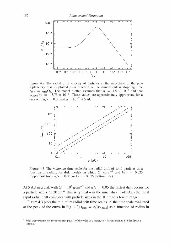
152 Planetesimal Formation
vv
Figure 4.2 The radial drift velocity of particles at the mid-plane of the pro-toplanetary disk is plotted as a function of the dimensionless stopping timeτfric = tfric�K. The model plotted assumes that η = 7.5 × 10⁻³ and thatvr,gas/vK = −3.75 × 10⁻⁵. These values are approximately appropriate for adisk with h/r = 0.05 and α = 10−2 at 5 AU.
Figure 4.3 The minimum time scale for the radial drift of solid particles as afunction of radius, for disk models in which � ∝ r−1 and h/r = 0.025(uppermost line), h/r = 0.05, or h/r = 0.075 (bottom line).
At 5 AU in a disk with � = 102 g cm−2 and h/r = 0.05 the fastest drift occurs fora particle size s � 20 cm.4 This is typical – in the inner disk (1–10 AU) the mostrapid radial drift coincides with particle sizes in the 10 cm to a few m range.
Figure 4.3 plots the minimum radial drift time scale (i.e. the time scale evaluatedat the peak of the curve in Fig. 4.2) tdrift = r/|vr,peak| as a function of radius in
4 With these parameters the mean-free path is of the order of a meter, so it is consistent to use the Epsteinformula.

4.3 Radial Drift of Solid Particles 153
the disk. Throughout the main planet-forming regions of the disk this time scale isextremely short – of the order of 103 yr or less for reasonable disk parameters. Thisis an important result, from which flow two robust conclusions:
• Planetesimal formation must be rapid, or very inefficient. This conclusionfollows from the fact that if growth through the cm–m-size scale were not veryrapid the vast majority of the solid material in the disk would drift toward the starto be evaporated in the hot inner regions of the protoplanetary disk.
• Radial redistribution of solids is very likely to occur. Radial flow of solidparticles on a time scale shorter than the disk lifetime occurs not just at the peakof the radial velocity drift curve, but also for substantially smaller and largerparticles. Local enhancements or depletions of solids (relative to the gas surfacedensity) will occur as a result.
These inferences follow from rather simple and well-understood physics, namelythe action of aerodynamic drag on particles orbiting within a sub-Kepleriangas disk.
4.3.1 Radial Drift with Coagulation
The size dependence of the radial drift velocity introduces a relative velocitybetween particles of different sizes, which can promote collisions and (possibly)growth via coagulation. We can use the same arguments that we employed to studycoagulation during vertical settling to assess whether this potentially beneficialaspect of radial drift outweighs the deleterious effects of radial drift in depleting thesolid surface density. As previously, we note that, in the limit where all collisionsare adhesive, the growth rate of a particle of radius s that collides primarily withsmaller particles5 as it drifts inward at the disk mid-plane is approximately
dm
dt= πs2|vr |fρ0, (4.43)
where f is the ratio of particle to gas density at z = 0, and ρ0, the mid-planegas density, is given by ρ0 = (1/
√2π)�/h. Comparing the growth time scale
tgrow = m/(dm/dt) to the drift time scale tdrift = r/|vr | we find that tgrow < tdrift forparticles of size
s <∼3f
4√
2π
(h
r
)−1�
ρm. (4.44)
If we assume that a modest amount of vertical settling has already taken place,appropriate values for the parameters in the inner disk might be f = 0.1,� = 103 g cm−2,ρm = 3 g cm−3, and h/r = 0.05. With these values we find
5 We assume that the particles in question have settled to z ≈ 0, and that their size is such that they lie on theleft-hand-side of the peak in the radial drift velocity curve plotted in Fig. 4.2.
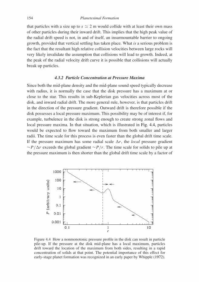
154 Planetesimal Formation
that particles with a size up to s � 2 m would collide with at least their own massof other particles during their inward drift. This implies that the high peak value ofthe radial drift speed is not, in and of itself, an insurmountable barrier to ongoinggrowth, provided that vertical settling has taken place. What is a serious problem isthe fact that the resultant high relative collision velocities between large rocks willvery likely invalidate the assumption that collisions will lead to growth. Indeed, atthe peak of the radial velocity drift curve it is possible that collisions will actuallybreak up particles.
4.3.2 Particle Concentration at Pressure Maxima
Since both the mid-plane density and the mid-plane sound speed typically decreasewith radius, it is normally the case that the disk pressure has a maximum at orclose to the star. This results in sub-Keplerian gas velocities across most of thedisk, and inward radial drift. The more general rule, however, is that particles driftin the direction of the pressure gradient. Outward drift is therefore possible if thedisk possesses a local pressure maximum. This possibility may be of interest if, forexample, turbulence in the disk is strong enough to create strong zonal flows andlocal pressure maxima. In that situation, which is illustrated in Fig. 4.4, particleswould be expected to flow toward the maximum from both smaller and largerradii. The time scale for this process is even faster than the global drift time scale.If the pressure maximum has some radial scale �r , the local pressure gradient∼P/�r exceeds the global gradient ∼P/r . The time scale for solids to pile up atthe pressure maximum is then shorter than the global drift time scale by a factor of
Figure 4.4 How a nonmonotonic pressure profile in the disk can result in particlepile-up. If the pressure at the disk mid-plane has a local maximum, particlesdrift toward the location of the maximum from both sides, resulting in a rapidconcentration of solids at that point. The potential importance of this effect forearly-stage planet formation was recognized in an early paper by Whipple (1972).

4.3 Radial Drift of Solid Particles 155
(r/�r)2. Another relevant circumstance in which inward drift can be halted occursin the presence of a massive planet, which as we will show later tends to create anannular gap in the disk surface density near the location of its orbit. A disk with sucha gap possesses a pressure maximum at the inner edge of the disk that is exterior tothe planet. Solids with some range of sizes would be expected to accumulate at thatlocation.
4.3.3 Particle Pile-up
Solids that experience radial drift can become concentrated (“pile up”) in the innerdisk (Youdin & Shu, 2002; Youdin & Chiang, 2004). The effect is present in thesimplest case where diffusion and inward drag by the mean flow are small, andfeedback of the particles on the gas can be neglected. The radial drift speed is thengiven by Eq. (4.40) as
vr � −ητfricvK, (4.45)
with η ∝ (h/r)2. For particles that are in the Epstein regime of drag, the stoppingtime in the mid-plane is (from Eqs. 4.13 and 2.19)
tfric = ρm
ρ0
s
vth=
√2π
ρmh
�
s
vth. (4.46)
Since h = cs/�, and cs and vth differ only by a numerical factor, we obtain
τfric = π
2
ρm
�s. (4.47)
Suppose now that the surface density profile of solids has attained a steady state,such that the mass flux Md is independent of radius. Then,
Md = −2πr�dvr = constant, (4.48)
and substituting for vr we find
�d
�∝
(h
r
)−2
r−1/2. (4.49)
For a disk with constant (h/r) the steady-state concentration of solids increasescloser to the star as r−1/2. In the case of a flaring disk with mid-plane tempera-ture profile, say, Tc ∝ r−1/2, the effect is stronger. A constant α model of sucha disk has a steady-state gas surface density profile � ∝ r−1, with the solidsfollowing �d ∝ r−2.
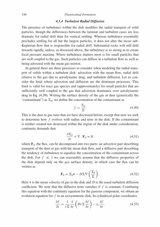
156 Planetesimal Formation
4.3.4 Turbulent Radial Diffusion
The presence of turbulence within the disk modifies the radial transport of solidparticles, though the differences between the laminar and turbulent cases are lessdramatic for radial drift than for vertical settling. Whereas turbulence essentiallyprecludes settling for all but the largest particles, it does not alter the mean sub-Keplerian flow that is responsible for radial drift. Substantial rocks will still driftinwards rapidly, unless, as discussed above, the turbulence is so strong as to createlocal pressure maxima. Where turbulence matters most is for small particles thatare well coupled to the gas. Such particles can diffuse in a turbulent flow as well asbeing advected with the mean gas motion.
In general there are three processes to consider when modeling the radial trans-port of solids within a turbulent disk: advection with the mean flow, radial driftrelative to the gas due to aerodynamic drag, and turbulent diffusion. Let us con-sider the limit where advection and diffusion are the dominant processes. Thislimit is valid for trace gas species and (approximately) for small particles that aresufficiently well coupled to the gas that advection dominates over aerodynamicdrag in Eq. (4.39). Writing the surface density of the gas or dust (generically the“contaminant”) as �d, we define the concentration of the contaminant as
f = �d
�. (4.50)
This is the dust to gas ratio that we have discussed before, except that now we seekto determine how f evolves with radius and time in the disk. If the contaminantis neither created nor destroyed within the region of the disk under consideration,continuity demands that
∂�d
∂t+ ∇ · Fd = 0, (4.51)
where Fd, the flux, can be decomposed into two parts: an advective part describingtransport of the dust or gas with the mean disk flow, and a diffusive part describingthe tendency of turbulence to equalize the concentration of the contaminant acrossthe disk. For f 1 we can reasonably assume that the diffusive properties ofthe disk depend only on the gas surface density, in which case the flux can bewritten as
Fd = �dv − D�∇(
�d
�
). (4.52)
Here v is the mean velocity of gas in the disk and D is the usual turbulent diffusioncoefficient. We note that the diffusive term vanishes if f is constant. Combiningthis equation with the continuity equation for the gaseous component, we obtain anevolution equation for f in an axisymmetric disk. In cylindrical polar coordinates
∂f
∂t= 1
r�
∂
∂r
(Dr�
∂f
∂r
)− vr
∂f
∂r. (4.53)

4.3 Radial Drift of Solid Particles 157
In common with the equation describing the settling of solid particles in a turbulentdisk (Eq. 4.27), this is an advection–diffusion equation, though here the advectivecomponent is due to the radial flow of the disk gas rather than settling. It is straight-forward to generalize this equation to account for the radial drift of larger particlesthat are imperfectly coupled to the gas – all that is required is to add an additionalflux to Eq. (4.52).
Equation (4.53) expresses a competition between diffusion, whose strengthdepends upon the turbulent diffusion coefficient D, and radial advection at avelocity vr . For a steady disk away from the boundaries, the radial velocity can bewritten in terms of the viscosity as
vr = −3ν
2r, (4.54)
so, as was the case with vertical settling, it is the ratio of the two transport coeffi-cients that is critical. This ratio is called the Schmidt number:
Sc ≡ ν
D. (4.55)
Diffusion becomes increasingly more important for low values of the Schmidtnumber.
In most cases of interest the contaminant equation (Eq. 4.53), where necessarymodified to allow for radial drift of particles, needs to be solved numerically alongwith the evolution equation for the gas surface density (Eq. 3.173). We can gainconsiderable insight into the general behavior, however, by examining the proper-ties of analytic solutions available for some special cases (Clarke & Pringle, 1988).Let us imagine a steady disk in which the surface density profile � ∝ r−γ (cor-respondingly, the viscosity scales with radius as ν ∝ rγ ). At some instant a ringof contaminant is injected into the disk at r = r0. Writing x = r/r0, we defineP(> x) to be the maximum fraction of contaminant that is ever at a disk radius ofx or larger. For γ = 2 this quantity can be expressed analytically in terms of thecomplementary error function6
P(> x) = 1
2erfc
[(3
2Sc ln x
)1/2]
. (4.56)
The solution is plotted for a variety of Schmidt numbers in Fig. 4.5. The extentto which contaminant can diffuse “upstream” (radially outward for a steady diskin which vr < 0) is a rather sensitive function of Sc. If the Schmidt number issignificantly greater than unity (i.e. the anomalous viscosity is greater than theturbulent diffusivity) almost no upstream diffusion occurs. Values of Sc = 0.33or lower, on the other hand, result in significant amounts of dust or gas diffusing
6 The complementary error function erfc(x) ≡ 1 − erf(x), where, erf(x) ≡ 2√π
∫ x0 e−t2
dt is the error function.

158 Planetesimal Formation
Figure 4.5 Demonstration of how the Schmidt number (Sc ≡ ν/D, the ratio ofthe turbulent viscosity to the turbulent diffusivity) affects the ability of a tracecontaminant (a minor gas species, or tightly coupled dust particles) to diffuseupstream against the inward flow of a steady accretion disk. The quantity P(> x)is the maximum fraction of contaminant, released at x = r/r0 = 1 in a steadydisk with � ∝ r−2, that ever reaches radius x or larger. Upstream diffusion issignificant only for Sc ≤ 1.
outward against the mean flow to large distances. Although the specific disk modelfor which the analytic solution applies is not very realistic (γ = 1 or γ = 3/2 aremore typical values than γ = 2) the basic conclusion holds more generally – theextent of outward diffusion depends on the Schmidt number.
4.4 Diffusion of Large Particles
From the preceding discussion it ought to be clear that determining the value ofthe Schmidt number is critical if we want to quantify either the vertical distributionof particles or their radial transport through the disk. If we restrict ourselves toconsidering gaseous species, or very small dust particles for which the dimension-less friction time τfric 1, the Schmidt number is best thought of as an intrinsicproperty of the turbulence present within the disk. To an order of magnitude itis normally reasonable to assume that Sc ∼ 1, but deviations from a Schmidtnumber of unity can be a factor of several in either direction and may differ betweenthe vertical and radial directions. Numerical simulations of the relevant turbulentprocesses are needed in order to quantify such departures.
For larger particles, the diffusion coefficient Dp is predicted to vary with theparticle size according to the value of the dimensionless friction time τfric.7 This
7 Confusingly, different authors use the term “Schmidt number” to refer to either ν/D or D/Dp. These aredifferent physical quantities. Here we define Sc to be the ratio of the kinematic viscosity in the disk to the
4.4 Diffusion of Large Particles 159
is easiest to visualize if we consider a large rock for which τfric � 1. A rock isnot swept up by turbulence in the relatively diffuse gas of the disk. Instead one canenvisage the rock as orbiting the star with a well-defined semi-major axis, eccen-tricity, and inclination. The rock is buffeted by random aerodynamic forces dueto the presence of turbulence, and these cause a slow drift in the orbital elements.Particles cannot plausibly diffuse faster than gas molecules, so we anticipate thatthe ratio D/Dp is bounded from below at unity. As particles become larger and thecoupling becomes weaker, the ratio will increase.
We can illustrate the dependence of Dp on τfric using simple arguments borrowedfrom Youdin and Lithwick (2007). We assume that the disk is turbulent, and that theturbulence can be described using the hydrodynamic picture of interacting eddiesdeveloped by Kolmogorov. The characteristic turnover time scale of the eddies iswritten in dimensionless form as
τeddy ≡ �teddy, (4.57)
exactly analogous to the definition of the dimensionless friction time τfric ≡ �tfric.The characteristic velocity of the turbulent fluctuations δvg is defined such that thegaseous diffusion coefficient
D = δv2g teddy. (4.58)
For simplicity we focus on the limit in which τfric � 1 and τeddy 1. In this regimeof friction time a particle on a noncircular or noncoplanar orbit executes (to leadingorder) epicyclic oscillations with a frequency κ = �. During each oscillation ofduration �−1 the particle receives N ∼ τ−1
eddy independent impulses, each impartinga velocity kick
δvp ∼ τeddy
τfricδvg. (4.59)
The kicks are independent, so they accumulate as a random walk. After a time �−1
δvp ∼ τeddy
τfricδvg
√N ∼
√τeddy
τfricδvg, (4.60)
and the particle has drifted a distance δl ∼ δvp�−1. Noting that the diffusion
coefficient (Eq. 4.58) can be generically rewritten in the form Dp ∼ δl2� we obtain,in the limit of large τfric, that Dp ∼ D/τ 2
fric. Since we have argued that Dp → D forτfric 1 we can guess a general expression for the ratio of the gas to the particlediffusion coefficients:
D
Dp∼ 1 + τ 2
fric. (4.61)
gaseous diffusion coefficient. In this section we discuss the relation between the gas and particle diffusivities,but refrain from giving that ratio a name.
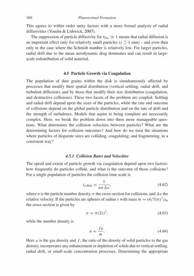
160 Planetesimal Formation
This agrees to within order unity factors with a more formal analysis of radialdiffusivities (Youdin & Lithwick, 2007).
The suppression of particle diffusivity for τfric � 1 means that radial diffusion isan important effect only for relatively small particles (s <∼ 1 mm) – and even thenonly in the case where the Schmidt number is relatively low. For larger particles,radial drift due to the mean aerodynamic drag dominates and can result in large-scale redistribution of solid material.
4.5 Particle Growth via Coagulation
The population of dust grains within the disk is simultaneously affected byprocesses that modify their spatial distribution (vertical settling, radial drift, andturbulent diffusion), and by those that modify their size distribution (coagulation,and destructive collisions). These two facets of the problem are coupled. Settlingand radial drift depend upon the sizes of the particles, while the rate and outcomeof collisions depend on the global particle distribution and on the rate of drift andthe strength of turbulence. Models that aspire to being complete are necessarilycomplex. Here, we break the problem down into three more manageable ques-tions. What determines the collision velocities between particles? What are thedetermining factors for collision outcomes? And how do we treat the situationswhere particles of disparate sizes are colliding, coagulating, and fragmenting, in aconsistent way?
4.5.1 Collision Rates and Velocities
The speed and extent of particle growth via coagulation depend upon two factors:how frequently do particles collide, and what is the outcome of those collisions?For a single population of particles the collision time scale is
tcollide = 1
nσ�v, (4.62)
where n is the particle number density, σ the cross-section for collisions, and �v therelative velocity. If the particles are spheres of radius s with mass m = (4/3)πs3ρm
the cross-section is given by
σ = π(2s)2, (4.63)
while the number density is
n = fρ
m. (4.64)
Here ρ is the gas density and f , the ratio of the density of solid particles to the gasdensity, incorporates any enhancement or depletion of solids due to vertical settling,radial drift, or small-scale concentration processes. Determining the appropriate
4.5 Particle Growth via Coagulation 161
value of �v is trickier. For small dust particles the dominant effect will be dueto Brownian motion, which, for a particle in thermal equilibrium with a gas attemperature T , introduces a random velocity of the order of (1/2)mv2 ∼ kBT .For particles of masses m1 and m2 the collision velocity in the Brownian motionregime is
�v =√
8kBT (m1 + m2)
πm1m2. (4.65)
The velocity is of the order of 0.1 cm s−1 for μm-sized particles in a gas atT = 300 K. In the simple case where all the particles have the same mass m1 =m2 = m, Eqs. (4.62) through (4.65) yield as an estimate of the collision time scale
tcollide = πρ3/2m s5/2
6√
3kBT fρ. (4.66)
Substituting typical numerical values for conditions in the inner protoplanetarydisk (a gas density ρ = 10−10 g cm−3, a dust to gas ratio f = 10−2, a materialdensity ρm = 3 g cm−3, and a temperature T = 300 K) we find
tcollide � 24
(s
1 μm
)5/2
yr. (4.67)
This is a very short time scale. Small dust particles will inevitably collide in theenvironment of the protoplanetary disk even if Brownian motion is the only processthat yields a relative velocity between particles. If the collisions are adhesive,particle growth will be rapid.
For larger particles the relative velocity is usually determined by a combinationof differential radial drift and velocity induced by imperfect coupling to turbulencewithin the disk. We can readily estimate the maximum values of these velocities.For radial drift, the peak drift speed for a single particle is (1/2)ηvK (Eq. 4.41),where η depends on the disk scale height through η = n(h/r)2 and n ∼ 3 is apre-factor that is of the order of unity. A rough estimate for the maximum collisionspeed due to differential radial drift between two large, but non-identically sizedparticles, is
�vdrift,max ∼ 1
4ηvK. (4.68)
In a disk with a mid-plane temperature profile T ∝ r−1/2 the radial dependence ofη cancels the radial dependence of vK. We obtain
�vdrift,max ∼ 25 m s−1, (4.69)
as an estimate of the peak collision velocity for two particles with τfric ∼ 1 driftingradially through the disk.

162 Planetesimal Formation
Similar values of the maximum collision velocity occur due to aerodynamiccoupling between particles and turbulent disk gas. A calculation by Ormel andCuzzi (2007) shows that the peak collision velocity in this limit is
�vt,max ∼ α1/2cs. (4.70)
In a disk with a mid-plane temperature profile T ∝ r−1/2 and a sound speed at 1 AUof 1 kms−1 we have
�vt,max ∼ 30( α
10−3
)1/2 ( r
AU
)−1/4m s−1. (4.71)
Consideration of these limiting cases makes clear that the range of particle collisionvelocities realized within protoplanetary disks is substantial. For micron-sized par-ticles, velocities of the order of 0.1–1 cm s−1 are reasonable, while particles withτfric ∼ 1 are expected to collide at speeds that are of the order of 10 m s−1 (withat most a weak radial dependence). Translating τfric ∼ 1 to a physical size requiresspecifying a disk model, but typically we would be thinking about s ∼ 1 m objectsat 1 AU (and throughout the disk interior to the snow line) and s ∼ 1 cm particlesat 100 AU.
4.5.2 Collision Outcomes
Determining the outcome of particle collisions as a function of particle size,composition, and relative velocity is one of the few aspects of planet formationwhere laboratory experiments – rather than theoretical calculations or astronomicalobservations – have primacy (a review of such experiments has been given byBlum & Wurm, 2008). The parameter space of interest is large. As we have noted,the relative velocities of bodies upon collision range from �v ∼ 0.1 cm s−1 (forBrownian motion of μm-sized dust particles) up to �v ∼ 10 − 100 m s−1 (for therelative velocity of meter-sized rocks subject to radial drift). Of equal importance isthe composition of the colliding objects, which here means not just their chemicalmakeup (silicates, water ice, etc), but also their internal structure (solid particles,or aggregates with varying shapes and strengths).
At an elementary level the considerations that determine whether two particlesstick upon collision are readily understood (e.g. Youdin, 2010). We consider twoidentical particles of mass m, which have a relative velocity (when they are wellseparated) of �v. Upon collision we assume that short-range adhesive forces act tobind the particles together with an energy �Es, and that a fraction f of the impactenergy is dissipated. Requiring that the particles remain bound (total energy lessthan zero) upon rebounding from each other, then yields a simple expression forthe maximum impact velocity that results in sticking:
1
4m�v2 ≤ f
(1 − f )|�Es|. (4.72)
For a given impact velocity, particles can therefore adhere to each other for one oftwo reasons. First, they may stick as a consequence of strong surface forces (i.e. the
4.5 Particle Growth via Coagulation 163
particles are physically “sticky”). This is most important for small particles. Thesurface forces that determine �Es act only over the small area that is physicallyin contact when the two particles collide, and hence increase with particle sizemore slowly than the kinetic energy on the left-hand-side. For larger particles, thedeclining ratio of surface area to mass means that surface forces become less impor-tant as a determining factor in collision outcomes, which are instead controlledincreasingly by the ability of particles to dissipate energy upon collision. Solidbodies fail to dissipate sufficient energy and tend to rebound rather than stick attypical collision velocities. It is likely, however, that small macroscopic particles(with sizes in the range between μm and cm) resemble a loosely bound aggregateof smaller dusty or icy particles. Such aggregates can dissipate a greater fractionof the kinetic energy of impact internally (i.e. f ∼ 1), and experiments confirmthat this can result in sticking probabilities that are substantially more favorable forongoing particle growth.
Guttler et al. (2010) mapped out the outcome of particle collisions underexpected protoplanetary disk conditions, using constraints from laboratory exper-iments that were available at the time. Full or partial coagulation, bouncing, andfragmentation are all possible for particle mass ratios and collision velocities foundin disks. In broad terms, however, there is a fragmentation threshold for silicateparticles at
�vf ≈ 1 m s−1, (4.73)
and net growth is hard to achieve if collision velocities substantially exceed thisvalue. Instead, a quasi-equilibrium is set up in which simultaneous coagulationand fragmentation processes balance. The resulting size distribution has most ofthe mass in the largest particles, which may be of mm- or cm-sized dimensions(Birnstiel et al., 2011).
Laboratory experiments on aggregates made up of μm- or sub-μm-sized silicateparticles are intended to represent conditions interior to the water snow line inprotoplanetary disks. Further out, water and other ices (such as CO) are the dom-inant species. Knowledge of collision outcomes in this regime is scarcer than forsilicates. Ices can have a fragmentation threshold that is substantially larger thansilicates (perhaps of the order of 10 m s−1, which approaches the peak collisionspeeds realized in disks; Gundlach & Blum, 2015). The fragmentation thresholdfor ice is, however, likely to be temperature dependent, and may be comparable tothe silicate value in the outer regions of the disk where the temperature is far belowthe sublimation temperature (and where other ice species are present).
4.5.3 Coagulation Equation
It is an observed fact that particles of μm and mm size coexist within protoplan-etary disks, and it is likely that at any time the size distribution includes physi-cally interesting numbers of particles spanning an even wider range of scales. For

164 Planetesimal Formation
representative particles of mass (m1,m2) collisions occur at a rate that dependsupon the number density of the colliding particles and their relative velocity, with avelocity that has both a mean value and a distribution. Several outcomes, includingfull or partial coagulation, bouncing, and fragmentation, depend upon the param-eters of the collision and the chemical and physical makeup of the particles. Amathematical way to handle this is based upon the coagulation equation developedby Smoluchowski (1916). The formalism that results is easy to state but difficult tosolve except by numerical means.
Suppose that at some time the number of solid particles per unit volume withmasses in the range between m and (m + dm) is n(m)dm. As time proceeds, thenumber of particles of mass m increases whenever there is an adhesive collisionbetween any two particles whose masses sum to m, and decreases whenever aparticle of mass m coagulates with any other particle. Mathematically,
∂n(m)
∂t= 1
2
∫ m
0A(m′,m − m′)n(m′)n(m − m′)dm′
− n(m)
∫ ∞
0A(m′,m)n(m′)dm′, (4.74)
where the factor of one-half eliminates double counting of the collisions thatincrease the number of particles of mass m. As written this equation is extremelygeneral, and it finds applications in physical chemistry, biology, and cosmology aswell as in planet formation. The physics of any specific application is encoded inthe reaction kernel A, which can be written in our case as
A(m1,m2) = P(m1,m2,�v)�v(m1,m2)σ (m1,m2). (4.75)
Here P(m1,m2,�v) is the probability that a collision between two particles ofmasses m1 and m2 leads to adhesion, �v is the relative velocity at collision, and σ isthe collision cross-section. It is straightforward to further generalize the coagulationequation to include fragmentation and/or populations of particles with differentphysical properties (e.g. some particles may be compact spheres, while others areporous or fractal aggregates).
The coagulation equation (Eq. 4.74) is also important in the theory of terrestrialplanet formation, and we defer detailed discussion of analytic solutions to the equa-tion until Section 5.5. Suffice to say that it has the form of an integro-differentialequation for the time evolution of the particle mass distribution, and that it isdifficult to solve. Two general points, however, are worth noting now. First, growthof particles of mass m is described by a weighted sum over all possible collisionsthat yield the correct total mass. This means that even if the kernel is near zerofor some combinations of masses (perhaps for near-equal mass collisions of meter-scale bodies), growth is still possible if there is a high probability that other types ofcollision lead to adhesion. Second, the sticking probability P is evidently of centralimportance when assessing whether growth can occur and how rapid the process
4.5 Particle Growth via Coagulation 165
is. In general P will be a function of the masses of the particles involved, theircollision velocities, and additional parameters describing the shape and strength ofthe objects.
The integro-differential nature of the coagulation equation is rather differ-ent from most equations encountered in astrophysics, but efficient numericaltechniques are available to solve it. (This is not a trivial business, and a goodliterature search is recommended before trying to develop your own scheme!) Thedimensionality of the problem becomes higher in situations where it is physicallynecessary to keep track of additional variables beyond mass, such as particleporosity or chemical composition. In these circumstances Monte Carlo methods,based on random sampling of representative particle collisions, are the simplestnumerical schemes.
4.5.4 Fragmentation-Limited Growth
The experimental result that particle growth is limited by fragmentation above athreshold collision velocity can be converted, with the aid of a disk model, intoan estimate of the maximum particle size. As an example, let us assume that weare dealing with small particles (τfric
<∼ 1) whose collision velocities are set byaerodynamic coupling to turbulence in the disk gas. An approximation for thepeak mutual collision velocity, valid if τfric is not too much less than unity, is(Ormel & Cuzzi, 2007)
�v2 � 3
2ατfricc
2s . (4.76)
Using the explicit relation between τfric and particle size (Eq. 4.13), and assumingthat the maximum particle size smax is set by the condition that �v = �vf, thefragmentation threshold, we find
�v2f � 3
2α
ρm
ρ
smax
vth�Kc2
s . (4.77)
At the disk mid-plane ρ = ρ0 = (1/√
2π)(�/h). Using this expression, the factthat h = cs/�K, and noting the numerical difference between the thermal speed vth
(Eq. 4.1) and the sound speed cs, we obtain
smax � 4
3π
�
αρm
�v2f
c2s
. (4.78)
This is an estimate for how large particles can grow if (a) there is a strict velocity-dependent threshold to growth (due to fragmentation or bouncing), and (b) particleshave enough time to reach the maximum before radial drift transports them to aplace where the physical conditions are different (Birnstiel et al., 2012; Pinillaet al., 2012). The most important radial scaling comes from the surface densityterm, so the prediction of this model is that smax ought to generally decrease with

166 Planetesimal Formation
orbital radius. Superimposed on that decrease there may be one or more jumpsat radial locations where different material properties lead to different thresholdvelocities.
In the absence of particle trapping at pressure maxima, radial drift can moveparticles inward on a time scale that is shorter than collisions grow them to themaximum size allowed by fragmentation. Because smax increases closer to the star,the drifting (and growing) particles may never reach the sizes that are in principlepermissible at any given radius. This situation – in which the particle size as afunction of orbital distance is limited by time rather than by material properties – isdescribed as drift-limited growth. Approximate expressions for the resulting parti-cle sizes can be derived in an analogous manner to the fragmentation-limited case(Birnstiel et al., 2012).
4.6 Gravitational Collapse of Planetesimals
Thus far we have assumed that the only important interactions between particlesare physical collisions, and that those particles are dynamically unimportant forthe evolution of the gas disk. These assumptions are valid for small dust particlesdistributed uniformly throughout the gas disk – since the total mass of solids isnegligible compared to the mass of gas at the epoch when the disk forms – but theymay be locally violated due to some combination of vertical settling, radial drift,and photoevaporation. If the solid particles start to play a dynamical role a numberof new physical effects may occur:
• Gravitational instability within a dense layer of particles located close to thedisk mid-plane. Safronov (1969) and, independently, Goldreich and Ward (1973)proposed that such an instability might result in the prompt formation of planetes-imals. Although it is now known that the simplest version of their theory, knownas the Goldreich–Ward mechanism, fails, closely related physical ideas remainimportant.
• Modification of the properties of turbulence within the gas due to feedback fromthe solid component.
• The existence of new two-fluid instabilities that arise because of the couplingbetween the solid and gaseous components. These might result in clumping ofthe solid particles (over and above over-densities that would occur if the solidswere passive tracers within the turbulent gas flow), and promote planetesimalformation either via direct collisions or via gravitational collapse.
We begin by analyzing the stability of a thin particle layer to gravitational collapse.The physical considerations are identical to those discussed heuristically in Sec-tion 3.4 for the stability of a gaseous disk, with the particle velocity dispersion σ
taking the place of the gas sound speed, and the control parameter is once againToomre’s Q (Eq. 3.62). Let us derive that result more formally.

4.6 Gravitational Collapse of Planetesimals 167
4.6.1 Gravitational Stability of a Particle Layer
We consider a razor-thin disk of particles with uniform surface density �0 andconstant velocity dispersion σ orbiting the star in circular orbits in the z = 0 plane.In cylindrical polar coordinates (r,φ,z) the density of the disk is given by
ρ0(r,φ,z) = �0δ(z), (4.79)
where δ(z) is a Dirac delta function, while the velocity field is
v0(r,φ,z) = (0,r�,0). (4.80)
Here � = �(r) is the angular velocity of the particles. The angular velocity neednot be Keplerian, but for circular orbits we require that the centrifugal force balancegravity. If the gravitational potential is �0,
�2r = −d�0
dr. (4.81)
Note that because of the assumptions of constant density and constant velocity dis-persion, the equivalent of a pressure gradient force does not enter into the problem.
To proceed we now make a number of simplifications. First, we assume thatcoupling of the particles to any gas present can be ignored. Second, we assumethat the particle layer can be treated as a fluid in which the two-dimensional soundspeed, defined in terms of the pressure p and surface density � in the usual way via
c2s ≡ dp
d�, (4.82)
is equivalent to the particle velocity dispersion σ . This is not formally correct,and it is not obvious that it is correct at all. If the particles are collisionless, their“pressure” need not be isotropic and their dynamics should be described not by thefluid equations but by the collisionless Boltzmann equation. It turns out, however,that the fluid and collisionless stability criteria are practically indistinguishable (see,e.g. Binney & Tremaine, 1987), with the fluid version being much easier to derive.Adopting the fluid description, the basic equations describing the dynamics of theparticle disk are the continuity and momentum equations, together with the Poissonequation for the gravitational field:
∂�
∂t+ ∇ · (�v) = 0, (4.83)
∂v∂t
+ (v · ∇)v = −∇p
�− ∇�, (4.84)
∇2� = 4πGρ. (4.85)
Our task is to determine, given these equations, the conditions under which theinitial equilibrium state of the disk (defined by Eqs. 4.79, 4.80, and 4.81) is stableagainst the effect of disk self-gravity, which unopposed would tend to result in the

168 Planetesimal Formation
particles gathering into dense clumps or rings. This can be accomplished with astandard linear stability analysis. We consider infinitesimal axisymmetric perturba-tions to the equilibrium state:
� = �0 + �1(r,t), (4.86)
p = p0 + p1(r,t), (4.87)
� = �0 + �1(r,t), (4.88)
v = v0 + [vr(r,t),δvφ(r,t),0
], (4.89)
that have a spatial and temporal dependence given by (using the surface density asan example)
�1(r,t) ∝ exp[i(kr − ωt)]. (4.90)
Here k is the spatial wavenumber of the perturbation (related to the wavelength viaλ = 2π/k) and ω is the temporal frequency. Ultimately, what we need to determineis whether there are values of k (i.e. spatial scales) for which ω is imaginary, sinceimaginary values of the frequency will result in exponentially growing perturba-tions. Making one further approximation, we assume that for the perturbations ofinterest
kr � 1. (4.91)
This amounts to considering disturbances that are small compared to the radialextent of the disk.
We now substitute the expressions for the surface density, pressure, gravitationalpotential, and velocity into the fluid equations, discarding any terms we encounterthat are quadratic in the perturbed quantities (this is a linear stability analysis). Forthe continuity equation this yields
−iω�1 + vr�0
(1
r+ ik
)= 0, (4.92)
which simplifies further in the local limit (kr � 1) to
−ω�1 + kvr�0 = 0. (4.93)
Deriving the analogous algebraic equations from the momentum equation requiresus to express the convective operator (v · ∇)v in cylindrical coordinates. This takesthe rather unwieldy form
(v · ∇)v =[vr
∂vr
∂r+ vφ
r
∂vr
∂φ+ vz
∂vr
∂z− v2
φ
r,
vr
∂vφ
∂r+ vφ
r
∂vφ
∂φ+ vz
∂vφ
∂z+ vrvφ
r,vr
∂vz
∂r+ vφ
r
∂vz
∂φ+ vz
∂vz
∂z
].
(4.94)
4.6 Gravitational Collapse of Planetesimals 169
With this in hand, the momentum equation reduces immediately to
−iωvr − 2�δvφ = − 1
�0
dp1
dr− d�1
dr, (4.95)
− iωδvφ + vr
[� + d
dr(r�)
]= 0, (4.96)
where the two equations come from the radial and azimuthal componentsrespectively.
The next step is to relate the perturbations in pressure and gravitational poten-tial expressed on the right-hand-side of Eq. (4.95) to perturbations in the surfacedensity. For the pressure term this is straightforward. Equation (4.82) implies that
1
�0
dp1
dr= 1
�0c2
s ik�1. (4.97)
Dealing with the potential perturbations requires more work. Starting from thelinearized Poisson equation,
∇2�1 = 4πG�1δ(z), (4.98)
we write out the Laplacian explicitly and simplify making use of the fact that forshort wavelength perturbations kr � 1. This yields a relation between the densityand potential fluctuations:
d2�1
dz2= k2�1 + 4πG�1δ(z). (4.99)
For z �= 0 the only solution to this equation that remains finite for large |z| hasthe form
�1 = C exp[−|kz|], (4.100)
where C remains to be determined. To do so we integrate the Poisson equationvertically between z = −ε and z = +ε:∫ +ε
−ε
∇2�1dz =∫ +ε
−ε
4πG�1δ(z)dz. (4.101)
Noting that both ∂2�1/∂x2 and ∂2�1/∂y2 are continuous at z = 0, whereas
∂2�1/∂z2 is not, we obtain
d�1
dz
∣∣∣∣+ε
−ε
= 4πG�1. (4.102)
Taking the limit ε → 0 we find that C = −2πG�1/|k|, and hence that the generalrelation between potential and surface density fluctuations on the z = 0 plane is
�1 = −2πG�1
|k| . (4.103)

170 Planetesimal Formation
Taking the radial derivative
d�1
dr= −2π ikG�1
|k| , (4.104)
which allows us to eliminate the potential from the right-hand-side of Eq. (4.95) infavor of the surface density. The result is
−iωvr − 2�δvφ = − 1
�0c2
s ik�1 + 2π ikG�1
|k| . (4.105)
Finally, we are ready to derive the functional relationship between ω and k, knownas the dispersion relation. Eliminating vr and δvφ between Eqs. (4.93), (4.96), and(4.105) we find that
ω2 = κ2 + c2s k
2 − 2πG�0|k|, (4.106)
where the epicyclic frequency κ is defined as
κ2 ≡ 4�2 + 2r�d�
dr. (4.107)
In a Keplerian potential κ2 = �2.The basic properties of the dispersion relation for a self-gravitating particle (or
gas) disk (Eq. 4.106) are readily apparent. Recall that for instability to occur, werequire that ω2 < 0 so that ω itself is imaginary and perturbations grow expo-nentially with time.8 Both rotation and pressure – the first and second terms onthe right-hand-side of the dispersion relation – are unconditionally positive and actas stabilizing influences, with rotation stabilizing all scales equally and pressurepreferentially stabilizing short-wavelength (large k) perturbations. Self-gravity, thethird term, is destabilizing with a spatial dependence (linear in k) that lies intermedi-ate between that of rotation and pressure. These dependencies are shown in Fig. 4.6.
Setting dω2/dk = 0, we find that the wavenumber of the minimum in ω2(k) isgiven by
kmin = πG�0
c2s
. (4.108)
If the minimum in the ω2(k) curve falls into the unstable region, modes withk � kmin will display the fastest exponential growth. The condition for the disk tobe marginally unstable to gravitational instability is then obtained by requiring thatω2(kmin) = 0. For a Keplerian disk instability requires that
Q ≡ cs�
πG�0< 1, (4.109)
8 There will also be exponentially decaying solutions, but the growing modes will rapidly dominate.

4.6 Gravitational Collapse of Planetesimals 171
Pressure
Rotation
Most unstable wavelengthGravity
Wavenumber, k
Figure 4.6 The dispersion relation (solid curve) for axisymmetric perturbationsto a self-gravitating razor-thin gaseous disk. The short-dashed line shows theboundary between instability (ω2 < 0) and stability (ω2 > 0). The long-dashed lines show the individual contributions from rotation (stabilizing at allwavenumbers), pressure (stabilizing at large wavenumber/short wavelength) andself-gravity (destabilizing).
where Q is customarily referred to as the “Toomre Q” parameter after AlarToomre’s 1964 paper. Up to numerical factors, the result matches that deducedusing time scale arguments in Section 3.4. Additional numerical factors arisewhen the analysis is generalized to allow for the possibility of nonaxisymmetricinstability within the disk. For nonaxisymmetric modes the control parameter isstill Q, but instability sets in more easily (i.e. at higher Q) and results in thedevelopment of spiral arms within the disk rather than the rings that would be theendpoint of the purely axisymmetric instability. In most circumstances the sub-tleties introduced by the presence of nonaxisymmetric modes are of only moderateimportance, and it suffices to note that the disk will become unstable to its ownself-gravity when
Q <∼ Qcrit, (4.110)
with Qcrit being of the order of, but slightly larger than, unity.

172 Planetesimal Formation
4.6.2 Application to Planetesimal Formation
With the mathematical formalities of disk instability in place we can proceed toconsider how this process might play a role in planetesimal formation. The basicidea, illustrated schematically in Fig. 4.7 involves three stages:
(1) Initially the solid component of the disk is well mixed with gas. The Q of thesolid component is very large and the effects of self-gravity play no role in theevolution.
(2) Over time the dust settles vertically to form a thin sub-disk of particles aroundthe z = 0 plane. As we have already noted, even the slightest breath of turbu-lence suffices to stir up dust particles, so substantial settling requires at leastsome collisional growth to have occurred. Radial drift can also contribute to anincrease in the mid-plane particle density in the inner disk.
(3) Due to some combination of high surface density and/or low velocity dis-persion, the particle sub-disk becomes unstable according to the Q criterion.This may lead to the formation of bound clumps of particles, which rapidlyagglomerate to form planetesimals.
Deferring for the moment the question of whether this sequence of events canplausibly occur, we can ask what would be the properties of planetesimals formed
hgasPrimordial disk
Particle settling + radial flow + growth
Fragmentation into planetesimals
Particle sub-disk
Figure 4.7 How planetesimals form within the classical Goldreich–Ward scenario.
4.6 Gravitational Collapse of Planetesimals 173
via gravitational instability? If the particle layer has velocity dispersion σ andsurface density �s its vertical scale-height will be
hd = σ
�, (4.111)
while the most unstable wavelength
λ ∼ 2π
kmin= 2σ 2
G�s. (4.112)
For Q = Qcrit these scales are comparable, so instability, if it occurs, results in thecollapse of relatively small patches of the particle layer into planetesimals.
The mass of clumps formed via gravitational instability is of the order of
mp ∼ πλ2�s ∼ 4π5G2Q4crit
�3s
�4. (4.113)
Adopting parameters that might be appropriate for the protoplanetary disk at 1 AU(�s = 10 g cm−2,Qcrit = 1) the estimated planetesimal mass is
mp(1 AU) ∼ 3 × 10¹⁸ g, (4.114)
which corresponds to a spherical body with a radius of 5–10 km. If we assume –rather unrealistically – that once gravitational instability of the particle layer setsin collapse occurs on the free-fall time scale, then the formation time is very short,being less than a year for the fiducial parameters above.
In principle a particle layer that fragments to form planetesimals could be com-posed of objects of any size, provided that the conditions for instability are met.The case that attracts greatest interest in the literature, however, is that where theparticles have sizes of the order of a cm or smaller. Such particles are small enoughnot to suffer the potentially devastating rapid radial drift of larger bodies, andthere does not appear to be any particular obstacle to forming them rapidly viapairwise collisions. Subsequent instability of a layer made of small particles thenhas the feature – understandably attractive to many authors – of rapidly formingplanetesimals in a way that bypasses all of the potential hurdles involved in particlegrowth through the meter-scale regime.
4.6.3 Self-Excited Turbulence
Since the surface density in solid material is typically only of the order of 1% ofthe gas surface density, a very thin particle layer is required in order for gravita-tional instability to set in. For example, if the surface density in solids at 1 AU is�s = 10 g cm−2, we require a velocity dispersion of σ � 10 cm s−1 in order to

174 Planetesimal Formation
attain Q = 1. If the gas disk has h/r = 0.05 at this radius, the relative thickness ofthe particle and gaseous disks is then
hd
h∼ 10−4. (4.115)
In the absence of gas, attaining such a razor-thin particle disk is not implausible –the vertical thickness of Saturn’s rings, for example, is of the order of only 10 m. Inthe gas-rich environment of the protoplanetary disk, however, we need to considercarefully whether turbulence will preclude the particle layer from ever becomingthin enough to become unstable.
Intrinsic disk turbulence provides one barrier to the development of very thinparticle layers. Equation (4.30) yields an estimate of the ratio of the thicknesses ofthe particle and gas disks as a function of α and the dimensionless friction time�tfric. From that analysis it is obvious that the classical Goldreich–Ward instabilitycannot work for small particles (those with �tfric 1 that have not yet grown tothe size where radial drift becomes rapid) unless α is very small. Fully turbulentregions of the disk are unpromising sites for planetesimal formation via gravita-tional instability.
One might argue, of course, that the mid-plane of the disk is not necessarilyintrinsically turbulent (e.g. the discussion in Section 3.6). Unfortunately, even ifthe gas disk on its own were laminar the presence of the particle layer tend wouldto excite turbulence, via the mechanism depicted in Fig. 4.8. The crucial physicalpoint is that for gravitational instability to occur we require that the local particledensity exceed the local gas density (by as much as two orders of magnitude if weadopt the parameters given above). Within the particle layer the gas is therefore sub-dominant to the particles, and the orbital velocity of the flow will be comparableto the Keplerian velocity. Just above the particle layer, on the other hand, the gasdominated disk orbits at slightly less than the Keplerian speed due to the influenceof radial pressure gradients. As a consequence there will exist a vertical shearwhich, if it is too large, will be unstable to the development of Kelvin–Helmholtz
vk
Gas
Particles + gas
Figure 4.8 How the presence of a dense particle disk results in excitation ofturbulence within the flow.
4.6 Gravitational Collapse of Planetesimals 175
instabilities. This self-excited turbulence can prevent the particle layer from eversettling to the point where self-gravity could set in (Cuzzi et al., 1993).
To estimate the seriousness of this impediment to planetesimal formation weneed to consider the hydrodynamic stability of a stratified shear flow. The simplestcase to analyze is that of a nonrotating flow (i.e. the Coriolis force is neglected)with a density profile ρ(z) and a velocity profile vφ(z).9 The flow is assumed to bein hydrostatic equilibrium with a vertical pressure gradient being balanced by thevertical component of gravity gz. Stability against shear instabilities in this situationis measured by the Richardson number
Ri ≡ −gzd ln ρ/dz
(dvφ/dz)2. (4.116)
A necessary condition for instability is that Ri < 0.25 somewhere within the flow.Let us evaluate the Richardson number across a particle layer of vertical height
hd, at radius r within a gas disk of scale-height h and in which the mid-planepressure varies as P ∝ r−n. We assume that gz is dominated by the vertical compo-nent of the star’s gravity, that the density in d ln ρ/dz is the total density (gas plusparticles), and that the velocity shear reflects the difference between the Keplerianvelocity and the gas disk velocity across the height of the layer. Collecting togetherpreviously derived results we then estimate these terms as
gz = �2hd, (4.117)
d ln ρ
dz= − 1
hd, (4.118)
(dvφ
dz
)2
= n2
4
(h
r
)4�2r2
h2d
. (4.119)
The resulting Richardson number is (adopting n = 3)
Ri � 0.25
(h/r
0.05
)−2 (hd/h
0.0375
)2
. (4.120)
Clearly, attaining the very thin layers needed to induce gravitational instabilityis rather difficult. As the particle layer settles toward the mid-plane, self-excitedturbulence is liable to set in long before Q ∼ 1.
The roadblock of self-excited turbulence largely excludes the classicalGoldreich–Ward mechanism as a viable planetesimal formation process. Whatsurvives in modern thinking is the key role of gravitational collapse, which canstill occur if the particle density is enhanced by processes other than just verticalsettling. Three potentially multiplicative processes can also occur:
9 As several authors have recently emphasized, this analysis is considerably too simple to yield an accurateanswer (Garaud & Lin, 2004; Gomez & Ostriker, 2005; Chiang, 2008). In more complete analyses the presenceof the Coriolis force tends to further destabilize the disk flow, while the presence of radial shear is a stabilizingeffect. The calculation presented here is intended only to illustrate the basic physical considerations at work.
176 Planetesimal Formation
• Large-scale enhancement (scales � h) due to the radial drift and pile-up ofparticles.
• Intermediate-scale (∼ h) concentration of solids, for example in zonal flows orvortices.
• Small-scale ( h) clustering from two-fluid instabilities present in disks.
We have already discussed the first two of these possibilities, which have in com-mon the fact that they involve the particle response to features (either the overallsurface density profile or localized structure) that are intrinsic properties of thegas disk. Two-fluid instabilities are qualitatively different, as they depend for theirexistence on the feedback momentum transport between solids and gas exerts onthe gas itself.
4.7 Streaming Instability
The streaming instability (Youdin & Goodman, 2005) is an instability of disksthat can be present whenever two phases or fluids (gas and solid particles) have amutual velocity and interact via aerodynamic forces. The instability grows on a timescale that is often intermediate between the dynamical and radial drift time scales,and leads to small-scale particle concentration. Strictly construed, the streaminginstability is a local linear instability of a highly simplified but mathematicallywell-defined system. The main interest in the instability, however, occurs becauseit offers a route to forming solid over-densities that are dense enough to collapsegravitationally to form planetesimals. As a result, the term “streaming instability” isalso used more loosely to refer to two-phase instabilities in more complex systems(for example systems where the solids are settling, or where the gas is intrinsicallyturbulent), and even to self-gravitating systems (where conceptually distinct insta-bilities can be present).
4.7.1 Linear Streaming Instability
The radial drift calculation of Section 4.3 considered a single particle interactingwith a background gas disk, and remains approximately valid for a population ofdrifting solids whose surface density is negligible compared to that of the gas. Thedrift solution needs to be modified if the surface density of the solids becomes non-negligible, because then the momentum transfer from the particles to the gas willmatter for the background disk structure.
A model for the drift of both solids and gas due to their aerodynamic interactionscan be derived by considering the gas to be incompressible, and the particles toform a fluid in which there are no pressure forces. The continuity and momentumequations for the aerodynamically coupled system are
∂ρd
∂t+ ∇ · (ρdvd) = 0, (4.121)

4.7 Streaming Instability 177
∇ · v = 0, (4.122)
∂vd
∂t+ vd · ∇vd = −�2
Kr − 1
tfric(vd − v) , (4.123)
∂v∂t
+ v · ∇v = −�2Kr + 1
tfric
ρd
ρ(vd − v) − ∇P
ρ, (4.124)
where the un-subscripted variables refer to the gas and the variables with a sub-script “d” refer to the particles. There is no vertical component of stellar gravityin these equations, nor is there any self-gravity of the fluids themselves. Solvingthem for a steady state, one obtains an axisymmetric flow describing the drift ofsolids and gas that is called the Nakagawa–Sekiya–Hayashi (NSH) equilibrium(Nakagawa et al., 1986).
Youdin and Goodman (2005) studied the linear stability of the NSH equilibriumto axisymmetric perturbations. The system exhibits instability for a wide range ofparameters (τfric, and the dust-to-gas ratio or “metallicity” ρd/ρ), provided thatthere is a nonzero mutual velocity between the particles and the gas in the equi-librium solution. Growth is generally faster for larger τfric, and for values of ρd/ρ
that are near but not equal to one. The instability does not have an intuitive physicalexplanation.
4.7.2 Streaming Model for Gravitational Collapse
The direct consequence of the streaming instability is that aerodynamically inter-acting solids in protoplanetary disks are likely to have a clumpy distribution onsmall spatial scales h. The instability can play a role in planetesimal formationif it generates over-densities that are large enough to initiate gravitational collapse.A necessary condition for collapse is that the density exceed the Roche density,such that self-gravity wins out over the tidal gravitational field of the star. For aclump of solids of mass m and radius r , orbiting at distance a from a star of massM∗, the tidal acceleration (i.e. the difference in force per unit mass between theedge and center of the clump) is
atidal = GM∗a2
− GM∗(a + r)2
� 2GM∗a3
r . (4.125)
Comparing this to the acceleration due to the clump’s own self-gravity,
agrav ∼ Gm
r2, (4.126)
we find that collapse will occur if
r <∼(
m
M∗
)1/3
a. (4.127)

178 Planetesimal Formation
Since the clump density ρ ∼ m/r3, an equivalent statement is that gravitationalcollapse requires that the solid density ρ must exceed the Roche density,
ρR ∼ M∗a3
= 6 × 10⁻⁷
(M∗M�
)( a
AU
)−3g cm−3. (4.128)
This is a high density. The gas density at the mid-plane of the disk at 1 AU mightbe of the order of 10−9 g cm−3 (assuming a gas surface density of 103 g cm−2 anda h/r ∼ 0.02), and vertically well-mixed solids would have a density roughly twoorders of magnitude less. Whether generated by the streaming instability or someother process, very high solid over-densities with �ρ/ρ ∼ 104 are needed beforeself-gravity becomes important enough to start gravitational collapse.
Yang et al. (2017) studied the properties of over-densities generated by thestreaming instability using numerical simulations that included the vertical com-ponent of stellar gravity but did not incorporate the self-gravity of the particlesthemselves. They found that for a given size of particle (expressed via thedimensionless stopping time τfric) the vertically integrated solid-to-gas ratio,Z ≡ �d/�, determined the strength of particle clumping. The strong particleclumping that is a prerequisite for gravitational collapse requires Z > Zcrit(τfric).The functional form of Zcrit can be fit by an approximate formula,
log Zcrit = 0.10(log τfric)2 + 0.20 log τfric − 1.76 (τfric < 0.1),
log Zcrit = 0.30(log τfric)2 + 0.59 log τfric − 1.57 (τfric > 0.1),
(4.129)
which is plotted in Fig. 4.9. The streaming instability is most effective at stronglyclumping solids in a broad region around τfric ∼ 0.1, but even for favorable parame-ters requires solid-to-gas ratios somewhat above the fiducial value of 0.01 to triggergravitational collapse (Johansen et al., 2009b).
In more complete models, the extent of particle clumping and gravitational col-lapse is likely to depend on a number of parameters. In addition to the particlestopping time, solid-to-gas ratio, and the velocity differential between solids andgas (all control parameters for even the linear theory), the relative strength of self-gravity and tidal shear, the strength of intrinsic disk turbulence, and the particle sizedistribution may play a role in determining the outcome. This parameter space isnot fully explored, but existing simulations, such as the one shown in Fig. 4.10,show that clumping can be strong enough to initiate gravitational collapse andthe formation of planetesimals, with a broad size distribution that extends to largemasses (Johansen et al., 2007).
4.8 Pathways to Planetesimal Formation
Planetesimal formation is the key step that links what is in principle directly observ-able – the distribution of highly mobile small solid particles with s <∼ mm inprotoplanetary disks – to the distribution of much less mobile km-scale bodies that

4.8 Pathways to Planetesimal Formation 179
Prompt streaming-initiatedgravitational collapse
Streaming over-densities too lowfor prompt gravitational collapse
fricfric
Figure 4.9 The critical solid to gas ratio Zcrit for prompt planetesimal formationis plotted as a function of the dimensionless stopping time τfric. For Z > Zcrit, thestreaming instability generates solid over-densities that are large enough to rapidlytrigger gravitational collapse. The critical curve is an analytic fit to numericalresults by Yang et al. (2017).
r0.2 h
Filaments of increasedparticle surface density
Formation of self-gravitatingparticle clumps
Gravitational collapse to planetesimals
f
Figure 4.10 The formation of planetesimals from the combined action of thestreaming instability and gravitational collapse. The streaming instability createsfilaments and clumps of solid particles, which can become dense enough tocollapse under self-gravity. From left to right, the panels show the time evolutionof the solid surface density from a three-dimensional local simulation (Abodet al, 2019).
is the effective initial condition for subsequent planet formation. We do not fullyunderstand how planetesimals form. To summarize the current state of knowledge,there appears to be no impediment to the rapid growth of dusty or icy particles up to
180 Planetesimal Formation
small macroscopic dimensions (s ∼ 1 mm). The growth mechanism at these scalesis pairwise collisions that result in sticking, and the time scale in the inner disk isa small fraction of the disk lifetime. The fact that dust is still present in the innerregions of disks with ages of several Myr suggests that regeneration of dust, viaerosive collisions, accompanies an overall trend toward growth.
Growth beyond the mm or cm size regime presents greater challenges. A strongargument can be made, based on the rapid radial drift of m-scale bodies due toaerodynamic forces, that growth all the way up to km-scale planetesimals must berapid, with a time scale less than 105 yr across the entire radial extent of the disk.Particle–particle collision velocities within turbulent disks appear to be too large toallow this growth to occur via continued pairwise collisions, certainly in the diskinterior to the snow line (if experiments based on silicates accurately represent thematerials found there), and probably in the icy regions further out. Gravitationalinstability provides a pathway to planetesimal formation that can bypass some ofthe scales where collisional growth is uncertain. A variety of processes, includingsettling, radial drift, and the streaming instability, can combine to concentrate solidssufficiently to trigger collapse.
The most promising mechanisms for particle growth and planetesimal formationhave short time scales, suggesting that the initial steps toward planet formationoccur early in the disk lifetime. It is less clear whether they operate with comparableefficiency everywhere in the disk, at specific discrete locations (such as near icelines), or at random places (such as in zonal flows or vortices). In the next chapterwe will adopt as a working hypothesis the idea that planetesimals typically formrapidly with a smooth radial distribution, and study how those planetesimals growinto larger bodies. This is the classical approach, but distinctly different modelscould also be consistent with what we know about planetesimal formation.
4.9 Further Reading
“The Multifaceted Planetesimal Formation Process,” A. Johansen et al. (2014), in Proto-stars and Planets VI, H. Beuther, R. S. Klessen, C. P. Dullemond, & T. Henning (eds.),Tucson: University of Arizona Press, p. 547.
“Forming Planetesimals in Solar and Extrasolar Nebulae,” E. Chiang & A. N. Youdin (2010),Annual Review of Earth and Planetary Sciences, 38, 493.
“The Growth Mechanisms of Macroscopic Bodies in Protoplanetary Disks,” J. Blum & G.Wurm (2008), Annual Review of Astronomy & Astrophysics, 46, 21.
5
Terrestrial Planet Formation
Once planetesimals have formed, further growth proceeds via a combination of twoprocesses. The first, planetesimal-driven growth, is a purely gravitational processin which the only role of the gas disk is to provide a modest degree of aerodynamicdamping of protoplanetary eccentricity and inclination. Planetesimal driven growthcan be studied using N-body simulations, which are indispensable for the latephases of final assembly of the Solar System’s terrestrial planets. Earlier phasescan also be approached using statistical methods, similar to that used in the kinetictheory of gases. In either treatment, the key questions are to determine the evolutionof self-consistent distributions of mass, eccentricity, and inclination, which are usedto determine the rate and outcome of collisions.
Classical models for terrestrial planet formation start from an initial conditionin which the surface density of planetesimals is specified, and include onlyplanetesimal-driven growth. This is not, however, the only possible way in whichgrowth may proceed. If a significant mass of small solid particles co-exist withplanetesimals and protoplanets – as seems very likely – bodies can grow in massas a consequence of the aerodynamically assisted accretion of the small solids.This process, called pebble accretion, is qualitatively distinct from planetesimalaccretion.
5.1 Physics of Collisions
The formation of terrestrial planets from planetesimals involves a cascade of pair-wise collisions. For the most part the gravity of growing planets is strong enoughthat we can assume that most of the mass of the two colliding bodies ends upagglomerating into a single larger object. For masses and collision velocities forwhich this is true we can gloss over the detailed physics of the collisions, and theprimary input to models of growth is the collision cross-section. The cross-sectionis enhanced by the gravity of the bodies (“gravitational focusing”), and modifiedas a result of the tidal gravitational field of the star. For small bodies and large
181
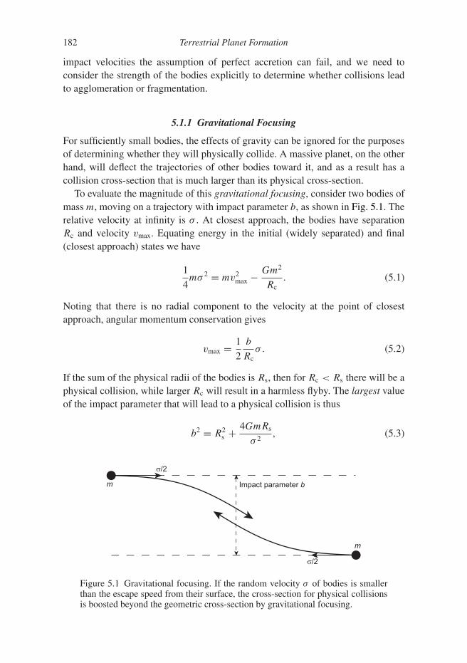
182 Terrestrial Planet Formation
impact velocities the assumption of perfect accretion can fail, and we need toconsider the strength of the bodies explicitly to determine whether collisions leadto agglomeration or fragmentation.
5.1.1 Gravitational Focusing
For sufficiently small bodies, the effects of gravity can be ignored for the purposesof determining whether they will physically collide. A massive planet, on the otherhand, will deflect the trajectories of other bodies toward it, and as a result has acollision cross-section that is much larger than its physical cross-section.
To evaluate the magnitude of this gravitational focusing, consider two bodies ofmass m, moving on a trajectory with impact parameter b, as shown in Fig. 5.1. Therelative velocity at infinity is σ . At closest approach, the bodies have separationRc and velocity vmax. Equating energy in the initial (widely separated) and final(closest approach) states we have
1
4mσ 2 = mv2
max − Gm2
Rc. (5.1)
Noting that there is no radial component to the velocity at the point of closestapproach, angular momentum conservation gives
vmax = 1
2
b
Rcσ . (5.2)
If the sum of the physical radii of the bodies is Rs, then for Rc < Rs there will be aphysical collision, while larger Rc will result in a harmless flyby. The largest valueof the impact parameter that will lead to a physical collision is thus
b2 = R2s + 4GmRs
σ 2, (5.3)
Impact parameter b
s/2
s/2
m
m
Figure 5.1 Gravitational focusing. If the random velocity σ of bodies is smallerthan the escape speed from their surface, the cross-section for physical collisionsis boosted beyond the geometric cross-section by gravitational focusing.
5.1 Physics of Collisions 183
which can be expressed in terms of the escape velocity from the point of contact,v2
esc = 4Gm/Rs, as
b2 = R2s
(1 + v2
esc
σ 2
). (5.4)
The cross-section for collisions is then
� = πR2s
(1 + v2
esc
σ 2
), (5.5)
where the term in brackets represents the enhancement to the physical cross-sectiondue to gravitational focusing. Clearly a planet growing in a “cold” planetesimal diskfor which σ vesc will grow much more rapidly as a consequence of gravitationalfocusing.
5.1.2 Shear versus Dispersion Dominated Encounters
Our derivation of the gravitational focusing term assumed that the only significantforces acting upon the colliding bodies were those due to their mutual gravity. Thisis a good approximation for studies, for example, of stellar collisions within a starcluster, but its legitimacy must always be evaluated carefully for planetary accretionwhere the gravity of the star is often important. What matters is not so much thetotal gravitational force due to the star, but rather the difference in the force thatis experienced by two bodies on similar orbits (i.e. the tidal gravitational field).Three-body dynamics is more complex than the two-body case, and in general isnot amenable to fully analytic treatments.
The condition for three-body dynamics to be important can be estimated froma time scale argument. We first estimate the radius within which the gravity of theprotoplanet, with mass Mp and orbital radius a, dominates over the stellar tidalfield. To do this we equate the orbital frequency of a protoplanet around the star(√
GM∗/a3) to that of a test particle orbiting the planet at radius r (√
GMp/r3).This yields an estimate of the radius of the Hill sphere:
rH ∼(
Mp
M∗
)1/3
a. (5.6)
Within rH two-body effects provide an adequate description of the dynamics.Likewise, we can define a characteristic velocity (the Hill velocity) as the orbitalvelocity around the protoplanet at the distance of the Hill radius:
vH ∼√
GMp
rH. (5.7)
If the random velocity σ of small bodies is large compared to the Hill velocity(σ > vH), then the rate with which they enter the Hill sphere and collide is deter-mined by two-body dynamics. This regime is described as dispersion dominated.

184 Terrestrial Planet Formation
y
x(-x , 0) (xp, 0)
r* rpr
M Mp
Figure 5.2 Geometry for the derivation of Hill’s equations.
If, conversely, σ < vH then three-body effects must be considered and the systemis said to be shear dominated.
The concept of the Hill sphere is important enough to be worth deriving morerigorously. To do so, we consider the motion of a test particle (a body whose massis negligible) in a binary system consisting of a star of mass M∗ and a protoplanetof mass Mp. We assume that the protoplanet orbits the star in a circular orbit withangular frequency �, and work in a co-rotating coordinate system such that the linejoining the star to the planet coincides with the x-axis. The origin of the coordinatesis taken to be the center of mass. This geometry is shown in Fig. 5.2. The motionof the test particle then obeys
r = −∇� − 2 (� × r) − � × (� × r), (5.8)
� = −GM∗r∗
− GMp
rp, (5.9)
where the dots denote time derivatives. Expressed in terms of componentswe have
x − 2�y − �2x = −G
[M∗(x + x∗)
r3∗+ Mp(x − xp)
r3p
], (5.10)
y + 2�x − �2y = −G
[M∗r3∗
+ Mp
r3p
]y, (5.11)
z = −G
[M∗r3∗
+ Mp
r3p
]z. (5.12)
These equations are valid for arbitrary masses M∗ and Mp. We can simplify themconsiderably, however, by considering the limit Mp M∗. In this limit |x∗| |xp|
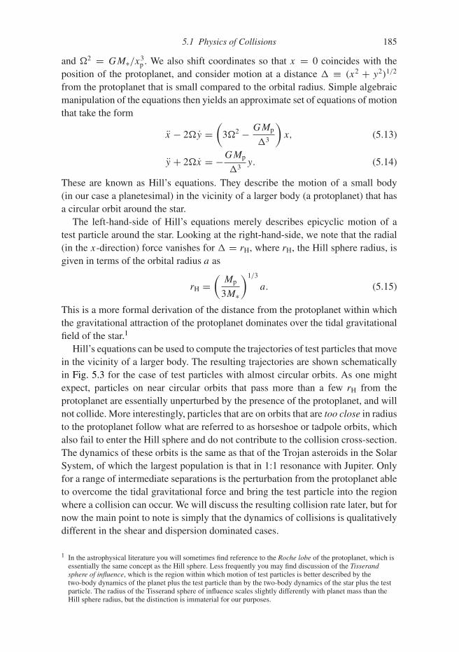
5.1 Physics of Collisions 185
and �2 = GM∗/x3p . We also shift coordinates so that x = 0 coincides with the
position of the protoplanet, and consider motion at a distance � ≡ (x2 + y2)1/2
from the protoplanet that is small compared to the orbital radius. Simple algebraicmanipulation of the equations then yields an approximate set of equations of motionthat take the form
x − 2�y =(
3�2 − GMp
�3
)x, (5.13)
y + 2�x = −GMp
�3y. (5.14)
These are known as Hill’s equations. They describe the motion of a small body(in our case a planetesimal) in the vicinity of a larger body (a protoplanet) that hasa circular orbit around the star.
The left-hand-side of Hill’s equations merely describes epicyclic motion of atest particle around the star. Looking at the right-hand-side, we note that the radial(in the x-direction) force vanishes for � = rH, where rH, the Hill sphere radius, isgiven in terms of the orbital radius a as
rH =(
Mp
3M∗
)1/3
a. (5.15)
This is a more formal derivation of the distance from the protoplanet within whichthe gravitational attraction of the protoplanet dominates over the tidal gravitationalfield of the star.1
Hill’s equations can be used to compute the trajectories of test particles that movein the vicinity of a larger body. The resulting trajectories are shown schematicallyin Fig. 5.3 for the case of test particles with almost circular orbits. As one mightexpect, particles on near circular orbits that pass more than a few rH from theprotoplanet are essentially unperturbed by the presence of the protoplanet, and willnot collide. More interestingly, particles that are on orbits that are too close in radiusto the protoplanet follow what are referred to as horseshoe or tadpole orbits, whichalso fail to enter the Hill sphere and do not contribute to the collision cross-section.The dynamics of these orbits is the same as that of the Trojan asteroids in the SolarSystem, of which the largest population is that in 1:1 resonance with Jupiter. Onlyfor a range of intermediate separations is the perturbation from the protoplanet ableto overcome the tidal gravitational force and bring the test particle into the regionwhere a collision can occur. We will discuss the resulting collision rate later, but fornow the main point to note is simply that the dynamics of collisions is qualitativelydifferent in the shear and dispersion dominated cases.
1 In the astrophysical literature you will sometimes find reference to the Roche lobe of the protoplanet, which isessentially the same concept as the Hill sphere. Less frequently you may find discussion of the Tisserandsphere of influence, which is the region within which motion of test particles is better described by thetwo-body dynamics of the planet plus the test particle than by the two-body dynamics of the star plus the testparticle. The radius of the Tisserand sphere of influence scales slightly differently with planet mass than theHill sphere radius, but the distinction is immaterial for our purposes.
186 Terrestrial Planet Formation
Figure 5.3 Trajectories of test particles on almost circular orbits that encounter aprotoplanet, as viewed in the frame co-rotating with the protoplanet. In the sheardominated regime particles whose orbits are too close to that of the protoplanetnever enter the latter’s Hill sphere and collide with the planet.
5.1.3 Accretion versus Disruption
When two initially solid bodies physically collide the outcomes can be dividedbroadly into three categories:
• Accretion. All or most of the mass of the impactor becomes part of the mass ofthe final body, which remains solid. Small fragments may be ejected, but overallthere is net growth.
• Shattering. The impact breaks up the target body into a number of pieces, butthese pieces remain part of a single body (perhaps after reaccumulating gravita-tionally). The structure of the shattered object resembles that of a rubble pile.
• Dispersal. The impact fragments the target into two or more pieces that do notremain bound.
These possibilities are illustrated in Fig. 5.4. If the target is itself a rubble pile thenthe first possibility – ending up with a solid body – is unlikely, but the collisioncould still either disperse the pieces or merely rearrange them into a larger but stillshattered object.
To delineate the boundaries between these regimes quantitatively, we consider animpactor of mass m colliding with a larger body of mass M at velocity v. We definethe specific energy Q of the impact via
Q ≡ mv2
2M, (5.16)
and express the thresholds for the various collision outcomes in terms of Q.Conventionally, we define the threshold for catastrophic disruption Q∗
D as theminimum specific energy needed to disperse the target in two or more pieces, withthe largest one having a mass M/2. Similarly Q∗
S is the threshold for shatteringthe body. More work is required to disperse a body than to shatter it, so evidentlyQ∗
D > Q∗S. It is worth keeping in mind that in detail the outcome of a particular
collision will depend upon many factors, including the mass ratio between the

5.1 Physics of Collisions 187
Accretion
Fragmentation +reaccretion
“Rubble pile”
Dispersal
Low
QH
igh
Q
Figure 5.4 Possible outcomes of collisions between bodies.
target and the impactor, the angle of impact, and the shape and rotation rate ofthe bodies involved. Quoted values of Q∗
D are often averaged over impact angles,but even when this is done the parameterization of collision outcomes in terms ofQ is only an approximation.
The estimated values of Q∗D for a target of a particular size vary by more than
an order of magnitude depending upon the composition of the body, which canbroadly be categorized into solid or shattered rock, and solid or porous ice. For anyparticular type of body, however, two distinct regimes can be identified:
• Strength dominated regime. The ability of small bodies to withstand impactwithout being disrupted depends upon the material strength of the object. Ingeneral the material strength of bodies declines with increasing size, owing tothe greater prevalence of defects that lead to cracks. In the strength dominatedregime Q∗
D decreases with increasing size.
• Gravity dominated regime. Large bodies are held together primarily by grav-itational forces. In this regime Q∗
D must at the very least exceed the spe-cific binding energy of the target, which scales with mass M and radius s asQB ∝ GM/s ∝ ρms2. In practice it requires a great deal more than this minimumamount of energy to disrupt the target – so QB is not a good estimate of Q∗
D – butnonetheless Q∗
D does increase with increasing size.
Although the transition between these regimes is reasonably sharp there is someinfluence of the material properties (in particular the shear strength) on the catas-trophic disruption threshold for smaller bodies within the gravity dominated regime.

188 Terrestrial Planet Formation
Values of Q∗S and Q∗
D can be determined experimentally for small targets(e.g. Arakawa et al., 2002). Experiments are not possible in the gravity dominatedregime, but Q∗
D can be estimated theoretically using numerical hydrodynam-ics (Benz & Asphaug, 1999; Leinhardt & Stewart, 2009) or (for rubble piles)rigid body dynamics simulations (Leinhardt & Richardson, 2002; Korycansky &Asphaug, 2006). A simple parameterization of the numerical results is as a brokenpower-law that includes terms representing the strength and gravity regimes:
Q∗D = qs
( s
1 cm
)a
+ qgρm
( s
1 cm
)b
. (5.17)
Often (but not always) Q∗D is averaged over impact geometry, and qs,qg,a, and b
are all constants whose values are derived by fitting to the results of numericalsimulations.
Benz and Asphaug (1999) and Leinhardt and Stewart (2009) determined thevalues of the fitting parameters in Eq. (5.17) from the results of an ensemble ofsimulations of impacts into icy or rocky targets. Their results are given in Table 5.1and plotted as a function of target size in Fig. 5.5. One observes immediatelythat the results for a particular target material vary with the impact velocity, andhence that Q∗
D is not the sole determinant of the outcome of collisions. There is,however, a clear transition between the strength and gravity dominated regimes,with the weakest bodies being those whose size is comparable to the cross-overpoint. The most vulnerable bodies are generally those with radii in the 100 m to1 km range. Just how vulnerable such bodies are to catastrophic disruption dependssensitively on their makeup, and it would be unwise to place too much trust inprecise numbers. As a rough guide, however, the weakest icy bodies have mini-mum Q∗
D ∼ 105 erg g−1, while the strongest conceivable planetesimals (unfracturedrocky bodies) have minimum Q∗
D > 106 erg g−1.As a reality check, we may note that asteroids in the main belt with e � 0.1
would be expected to collide today with typical velocities of the order of 2 km s−1.
Table 5.1 Parameters for the catastrophic disruption threshold fitting formula(Eq. 5.17), which describes how Q∗
D scales with the size of the target body. Thequoted values were derived by Benz and Asphaug (1999) and Leinhardt andStewart (2009) using numerical hydrodynamics simulations of collisions, whichare supplemented in the strength dominated regime by experimental results.
v qs qg
(km s−1) (erg g−1) (erg cm3 g−2) a b
Ice (weak) 1.0 1.3 × 10⁶ 0.09 −0.40 1.30Ice (strong) 0.5 7.0 × 10⁷ 2.1 −0.45 1.19Ice (strong) 3.0 1.6 × 10⁷ 1.2 −0.39 1.26Basalt (strong) 3.0 3.5 × 10⁷ 0.3 −0.38 1.36Basalt (strong) 5.0 9.0 × 10⁷ 0.5 −0.36 1.36

5.1 Physics of Collisions 189
Gravity
Material strength
(
)
Radius of target body (cm)
Figure 5.5 The specific energy Q∗D for catastrophic disruption of solid bodies
is plotted as a function of the body’s radius. The solid and short-dashed curvesshow results obtained using fits to theoretical calculations for impacts into“strong” targets by Benz and Asphaug (1999). The long-dashed curve showsthe recommended curve for impacts into “weak” targets from Leinhardt andStewart (2009), derived from a combination of impact experiments and numericalsimulations. In detail the solid curves show results for basalt at impact velocitiesof 5 km s−1 (upper curve) and 3 km s−1 (lower curve). The short-dashed curvesshow results for water ice at 3 km s−1 (the lower curve for small target sizes)and 0.5 km s−1 (upper curve for small target sizes). The long-dashed curve showsresults for normal impacts into weak water ice targets at 1 km s−1.
For a mass ratio m/M = 0.1 the specific energy of the collision is then aroundQ = 2 × 10⁹ erg g−1, which from Fig. 5.5 is sufficient to destroy even quite largesolid bodies with s � 100 km. This is consistent with the observation of asteroidfamilies, and the interpretation of such families as collisional debris. Evidently therandom velocities that characterize collisions must have been much smaller duringthe epoch of planet formation if we are to build large planets successfully out ofinitially km-scale planetesimals.
The collision model described above is quite basic. Subsequent work showsthat momentum, rather than specific energy, controls the outcome in many gravitydominated collisions (Leinhardt & Stewart, 2012). The use of the most up-to-datecollision models is highly recommended for any quantitative applications.

190 Terrestrial Planet Formation
5.2 Statistical Models of Planetary Growth
The basic assumption underlying statistical models of planetary growth is that thenumber of bodies is large enough that the population can be described by one ormore probability distributions that encode the probability that a body has a specifiedmass, inclination, and eccentricity. The details of actual orbits are assumed to beunimportant, and accordingly the distribution of the longitude of pericenter and thelongitude of the ascending node is taken to be uniform. For bodies of a given massthe population is then described by the distribution of Keplerian orbital elementsf (e,i), which can be regarded as the analog of the Maxwellian distribution ofvelocities for particles in a gas. Numerical experiments show that the appropriatedistribution that is set up as a result of gravitational interactions among a populationof bodies is a Rayleigh distribution. Specifically, for a population of planetesimalsof mass m and local surface density �p, the probability distribution of eccentricityand inclination takes the form
f (e,i) = 4�p
m
ei
〈e2〉〈i2〉 exp
[− e2
〈e2〉 − i2
〈i2〉], (5.18)
where 〈e2〉 and 〈i2〉 are the mean square values of the eccentricity and inclination,respectively (Lissauer, 1993). This distribution is equivalent to a Gaussian distri-bution of the random components (vr,vz, and δvφ = vφ − vK) of planetesimalvelocities
f (z,v) = ��p
2π2mσ 2r σ 2
z
exp
[−(v2
r + 4δv2φ)
2σ 2r
− (v2z + �2z2)
2σ 2z
], (5.19)
where the velocity dispersions σr and σz in the radial and vertical direction arerelated to the mean square eccentricities and inclinations via
σ 2r = 1
2〈e2〉v2
K, (5.20)
σ 2z = 1
2〈i2〉v2
K. (5.21)
One should note that the exact conversion between orbital elements and the randomcomponents of the velocity depends upon the problem under study. The definitionsgiven in Eq. (5.21) are appropriate for converting between mean square orbitalelements and velocity dispersions in the planetesimal distribution function, but forother applications different formulae are needed. For a single planetesimal witheccentricity e and inclination i at least three slightly different definitions of the“random velocity” σ can be useful (Lissauer & Stewart, 1993):
(1) The planetesimal velocity relative to a circular orbit with i = 0 with the samesemi-major axis
σ = (e2 + i2)1/2vK. (5.22)

5.2 Statistical Models of Planetary Growth 191
(2) The planetesimal velocity relative to the local circular orbit with i = 0
σ =(
5
8e2 + 1
2i2
)1/2
vK. (5.23)
(3) The planetesimal velocity relative to other planetesimals
σ =(
5
4e2 + i2
)1/2
vK. (5.24)
Yet more variations on these expressions arise due to the need to average overthe planetesimal distribution when calculating, for example, the collision rates ofplanetesimals with protoplanets.
Very often the physics of the excitation and damping of e and i is such that thevelocity distribution closely approximates an isotropic form. In this limit
〈e2〉1/2 = 2〈i2〉1/2, (5.25)
and the problem has one fewer degree of freedom. Whether or not we make thisassumption, however, our task is to calculate, for a given distribution of e and i,the rate of collisions while accounting properly for the effects of both gravitationalfocusing and three-body dynamics. Having done this we then need to consider themechanisms that determine appropriate values for 〈e2〉 and 〈i2〉.
5.2.1 Approximate Treatment
Simple results for the growth rate of protoplanets can readily be derived for thedispersion dominated regime. Let us assume that a relatively massive body of massM , physical radius Rs, and surface escape speed vesc is embedded within a swarm ofsmaller planetesimals. The planetesimal swarm has a local surface density �p anda velocity dispersion σ (assumed here to be isotropic so that no distinction betweenσr and σz is needed). The vertical scale-height of the swarm is then hp � σ/� andits volume density is
ρsw � �p
2hp. (5.26)
The statistical (or “particle in a box”) estimate for the growth rate of the massivebody is then simply the product of the density of the planetesimal swarm, theencounter velocity at infinity, and the collision cross-section � (Eq. 4.63):
dM
dt= ρswσπR2
s
(1 + v2
esc
σ 2
). (5.27)
Substituting for ρsw and hp we find that
dM
dt=
√3
2�p�πR2
s
(1 + v2
esc
σ 2
), (5.28)

192 Terrestrial Planet Formation
where the numerical pre-factor, which we have not derived, is correct for anisotropic velocity dispersion (Lissauer, 1993). The inverse scaling of the densitywith the velocity dispersion results in a cancellation of the direct effect of thevelocity dispersion, which enters only via the gravitational focusing term.
Two simple solutions to this equation give insight into the properties of moresophisticated models of planetary growth. First, we assume that the gravitationalfocusing factor,
Fg =(
1 + v2esc
σ 2
), (5.29)
is a constant, and that the surface density of the planetesimal swarm does not changewith time. In this limit the equation for the growth of the protoplanet’s radius,
dRs
dt=
√3
8
�p�
ρmFg, (5.30)
where ρm is the density of the protoplanet, can be trivially integrated. We find that
Rs ∝ t, (5.31)
and the radius grows at a linear rate. For an icy body with ρm = 1 g cm−1 at 5.2 AU(the current orbital radius of Jupiter),
dRs
dt≈ 1
(�p
10 g cm−2
)Fg cm yr−1. (5.32)
Unless gravitational focusing is dominant this is a very slow growth rate. At thisrate it would take 10 Myr – as long as or longer than the lifetime of typicalprotoplanetary disks – to grow a solid body up to a size of 100 km. We concludeimmediately that to build large bodies in the outer regions of the protoplanetary disklarge gravitational focusing enhancements to the cross-section are unavoidable.
Given the necessity of gravitational focusing, the other obvious limit to consideris that in which vesc � σ . In this regime
Fg � v2esc
σ 2= 2GM
σ 2Rs, (5.33)
and the rate of growth of the protoplanet mass becomes
dM
dt=
√3πG�p�
σ 2MRs = kM4/3, (5.34)
where k is a constant if the properties of the planetesimal swarm are fixed (i.e. ifthe growing protoplanet neither excites the velocity dispersion nor consumes asignificant fraction of the planetesimals). If under these conditions we consider thegrowth of two bodies with masses M1 and M2 such that M1 > M2 we find that
dM1/M1
dM2/M2= R1
R2> 1. (5.35)
5.2 Statistical Models of Planetary Growth 193
The initially more massive body grows faster than its less massive cousin, bothabsolutely and as measured by the ratio of masses M1/M2. This phenomenonis called runaway growth, and it allows for much more rapid formation of largebodies. Indeed, if we formally integrate Eq. (5.34) for a fixed planetesimal velocitydispersion we obtain
M(t) = 1
(M−1/30 − k′t)3
, (5.36)
where k′ is a constant. The planet attains an infinite mass at a finite time. In realitythis singularity is avoided because the feedback from the growing planet resultsin an increase of the planetesimal velocity dispersion, which slows growth. Thephysical lesson, however, is correct – gravitational focusing can drive runawaygrowth and rapid formation of large bodies.
5.2.2 Shear and Dispersion Dominated Limits
In the dispersion dominated limit the approximate treatment leading to Eq. (5.28)suffices to expose most of the important physics. The shear dominated limit istrickier to analyze, and in general there is no alternative but to use the results ofthree-body numerical experiments or fitting formulae derived from such exper-iments. To gain some analytic insight into the important processes we contentourselves here with an approximate treatment that is a simplified version of thatgiven by Greenberg et al. (1991). The calculation has two parts. First, we estimatethe width of the annulus (described as the “feeding zone”) surrounding the proto-planet within which planetesimals can be diverted on to trajectories that enter theHill sphere. Second, we assess the fraction of incoming planetesimals that actuallyimpacts the protoplanet.
To derive the width of the feeding zone we consider the limit in which the grow-ing protoplanet, of mass M , has a circular orbit. We assume that the planetesimalslikewise have very small eccentricities, so that we are firmly in the shear dominatedregime. A planetesimal whose orbit differs from that of the protoplanet by �a mustthen have its eccentricity excited to
e ≈ �a
a(5.37)
if it is to be diverted on to a trajectory that would approach the planet.Let us now evaluate the impulse that the planetesimal receives as it passes by the
protoplanet. The strongest perturbations occur while the two bodies are separatedby an azimuthal distance of �a or less, which persists for a time interval δt = 4/�.The impulse imparted to the planetesimal is then
δv ≈ 4
�
GM
(�a)2, (5.38)
194 Terrestrial Planet Formation
which corresponds to an eccentricity of
e ≈ 4
�2a
GM
(�a)2. (5.39)
Equating this value of the eccentricity to that required in order to yield an approachtrajectory (Eq. 5.37) we find that the outer edge of the feeding zone is delimited bya half-width2
�a �(
4M
M∗
)1/3
a = 2.3 rH, (5.40)
where the Hill sphere radius rH is defined by Eq. (5.15).Planetesimals with orbits as far away from the protoplanet as (a − �a) and
(a + �a) can be deflecting on to approach trajectories. However, not all orbitswithin the feeding zone permit close approaches. As illustrated in Fig. 5.3,those planetesimals whose orbits are too close to that of the protoplanet describehorseshoe orbits that never encounter the Hill sphere. Roughly speaking, thoseplanetesimals with semi-major axes between (a − �a/2) and (a + �a/2) areprotected from encounters. This reduces the effective width of the feeding zonefrom 2�a to �a. The typical planetesimal that can take part in the feeding flow isthen at a radial distance of 0.75�a from the protoplanet. In the frame rotating withthe protoplanet, the average relative velocity of approach for a planetesimal thatwill enter the Hill sphere is then
vshear = a
∣∣∣∣d�
da
∣∣∣∣ 3
4�a = 9
8��a. (5.41)
Combining the results for the effective width of the feeding zone and the approachvelocity we obtain
dMH
dt= 9
8��a�p�a, (5.42)
as the rate at which mass flows toward the protoplanet from the planetesimal diskin the shear dominated regime. Although we have not proved it here, this mass fluxthat is diverted toward the planet is to a good approximation also the mass flux thatenters the Hill sphere around the protoplanet.
The planetesimals that flow into the Hill sphere do so with typical encountervelocities that are (using Eq. 5.37) of the order of
venc ∼ evK ∼ ��a. (5.43)
Since �a scales as the Hill sphere radius the mass ratio of the protoplanet to the starenters this expression only weakly, as the one-third power. Once the planetesimals
2 This is an approximate derivation that happens to give an answer that is quite close to that derived fromnumerical experiments. Equally valid approximate treatments will all yield slightly different numerical factors.

5.2 Statistical Models of Planetary Growth 195
have entered the Hill sphere the collision cross-section with the protoplanet canbe evaluated using two-body dynamics. Provided that the half-thickness of theincoming planetesimal flow exceeds the gravitational capture radius
ai > Rcapture, (5.44)
where
Rcapture = Rs
(1 + v2
esc
v2enc
)1/2
, (5.45)
the collision cross-section takes the same form as in the dispersion dominated limit:
� = πR2s
(1 + v2
esc
v2enc
). (5.46)
Simple geometry, depicted in Fig. 5.6, then allows us to determine the fraction ofplanetesimals entering the Hill sphere that go on to impact the protoplanet. Thisfraction is
f ≈ �
(2rH)(2ai). (5.47)
Collecting together results, the rate at which the protoplanet grows via accretion ofplanetesimals in the shear dominated regime is the product of this fraction with themass flow rate into the Hill sphere (Eq. 5.42):
dM
dt= 9
32
(�a)2
airH�p�πR2
s
(1 + v2
esc
v2enc
). (5.48)
z
rH
Captureradius
2ai
Figure 5.6 An edge-on view showing the flow of planetesimals into the proto-planet’s Hill sphere in the shear dominated regime. In the limit depicted here,the vertical thickness of the planetesimal disk exceeds the capture radius of theprotoplanet and the three-dimensional formula for gravitational focusing describesthe cross-section. If the disk is very thin a different regime of essentially two-dimensional accretion applies.

196 Terrestrial Planet Formation
Although this expression is superficially similar to the result that we deducedin the dispersion dominated regime (Eq. 5.28) there are a number of importantdifferences. First, the gravitational focusing term within the parentheses no longerdepends upon the random velocities of the planetesimals, but rather on the ratiobetween the escape velocity and the speed at which planetesimals enter the Hillsphere. Since v2
enc ∝ r2H ∝ M2/3, while v2
esc ∝ M , there is a partial cancellation ofthe mass dependence of the gravitational focusing term. Second, there is an explicitdependence on the vertical thickness of the planetesimal swarm, dM/dt ∝ 1/i. Theeccentricity is formally irrelevant, although it will often be the case that the eccen-tricities and inclinations of the planetesimals continue to obey the relation e ∼ 2i.
The above analysis was predicated on the assumption that ai > Rcapture. If theplanetesimal disk is extremely cold and thin this assumption can be violated,and there is a further transition from the three-dimensional accretion geometrydiscussed above to an essentially two-dimensional planar flow. In the very thin disklimit the rate at which planetesimals enter the Hill sphere remains unaltered, butthe fraction of those planetesimals that are accreted becomes
f ≈ Rcapture
rH. (5.49)
The protoplanet growth rate in this regime contains no dependence upon eithere or i.
The parameters that control the growth rate of the protoplanet are different inthe shear and dispersion dominated limits, and hence there is no universality to thetransition between the different regimes. In particular, the switch from dispersion toshear domination does not occur at a universal value of the gravitational focusingfactor. Figure 5.7 shows the dependence of the collision cross-section (normalizedto the geometric cross-section) as a function of the ratio vesc/σ (after Greenberget al., 1991). This plot is constructed for specific protoplanet parameters assumingthat vesc remains fixed, while σ is varied maintaining e = 2i. In this case, andtypically, four regimes can be identified:
• For vesc/σ < 1 gravitational focusing is irrelevant, and growth occurs in thedispersion dominated regime according to the geometric cross-section.
• Once vesc/σ > 1 gravitational focusing becomes significant and rapidly comes todominate the cross-section, which increases quadratically with vesc/σ whilst weremain dispersion dominated.
• Exiting the dispersion dominated regime the growth of the cross-section firststeepens, before increasing more slowly (as 1/σ ) in the shear dominated regime.
• Finally, the thickness of the disk falls below the scale of the capture radius Rcapture.In this thin disk regime the effective cross-section is constant.
Computations of the growth rate based on numerical integrations of test particles inthe gravitational field of the protoplanet and the star show, not unexpectedly, thatthe transitions between these regimes occur quite smoothly.
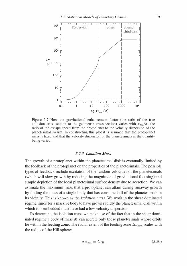
5.2 Statistical Models of Planetary Growth 197
Dispersion Shear Shear/thin†disk
Figure 5.7 How the gravitational enhancement factor (the ratio of the truecollision cross-section to the geometric cross-section) varies with vesc/σ , theratio of the escape speed from the protoplanet to the velocity dispersion of theplanetesimal swarm. In constructing this plot it is assumed that the protoplanetmass is fixed and that the velocity dispersion of the planetesimals is the quantitybeing varied.
5.2.3 Isolation Mass
The growth of a protoplanet within the planetesimal disk is eventually limited bythe feedback of the protoplanet on the properties of the planetesimals. The possibletypes of feedback include excitation of the random velocities of the planetesimals(which will slow growth by reducing the magnitude of gravitational focusing) andsimple depletion of the local planetesimal surface density due to accretion. We canestimate the maximum mass that a protoplanet can attain during runaway growthby finding the mass of a single body that has consumed all of the planetesimals inits vicinity. This is known as the isolation mass. We work in the shear dominatedregime, since for a massive body to have grown rapidly the planetesimal disk withinwhich it is embedded must have had a low velocity dispersion.
To determine the isolation mass we make use of the fact that in the shear domi-nated regime a body of mass M can accrete only those planetesimals whose orbitslie within the feeding zone. The radial extent of the feeding zone �amax scales withthe radius of the Hill sphere:
�amax = CrH. (5.50)
198 Terrestrial Planet Formation
For planetesimals on initially circular orbits the width of the feeding zone can beestimated by evaluating the maximum separation for which collisions are possiblewithin the context of the restricted three-body problem. This yields C = 2
√3
(Lissauer, 1993).3 The mass of planetesimals within the feeding zone is
2πa · 2�amax · �p ∝ M1/3. (5.51)
Note the one-third power of the planet mass, which arises from the mass depen-dence of the Hill radius. As a planet grows its feeding zone expands, but the massof new planetesimals within the expanded feeding zone rises more slowly thanlinearly. We thus obtain the isolation mass by setting the protoplanet mass equalto the mass of the planetesimals in the feeding zone of the original disk:
Miso = 4πa · C
(Miso
3M∗
)1/3
a · �p, (5.52)
which gives
Miso = 8√3π3/2C3/2M−1/2
∗ �3/2p a3. (5.53)
Evaluating this expression in the terrestrial planet region, taking a = 1 AU,
�p = 10 gcm−2,M∗ = M�, and C = 2√
3 we obtain
Miso � 0.07 M⊕. (5.54)
Isolation is therefore likely to occur late in the formation of the terrestrial planets.Repeating the estimate for the conditions appropriate to the formation of Jupiter’score, using �p = 10 g cm−2 as adopted by Pollack et al. (1996) gives
Miso � 9 M⊕. (5.55)
This estimate is comparable to or larger than the current best determinations for themass of the Jovian core. Full isolation may or may not be relevant to the formationof Jupiter and the other giant planets, depending upon the adopted disk model.
5.3 Velocity Dispersion
The random velocities of bodies during planet formation are determined by acompetition between excitation and damping processes. Several processes can beimportant:
• Viscous stirring. The random motions of a population of planetesimals thatare initially in a cold disk will be excited by the cumulative effect of weakgravitational encounters. The increase in the random energy of the bodies comes
3 This is larger than the value (C � 2.3) that we derived in Section 5.2.2 because here we consider allplanetesimals that are not dynamically forbidden from eventually encountering the protoplanet, whereaspreviously we counted only those that would be deflecting into the Hill sphere on an orbital time scale.

5.3 Velocity Dispersion 199
ultimately from the orbital energy. This is the only excitation process that operateswithin a disk composed of equal mass bodies.
• Dynamical friction. Gravitational scattering behaves somewhat differently in thecase where there is a spectrum of masses. The tendency for the system to seekequipartition of energy between the particles results in a transfer of energy frommassive bodies to less massive ones, and the development of a mass-dependentvelocity dispersion.
• Gas drag. Aerodynamic drag, although much weaker for planetesimals than formeter-scale bodies, continues to damp both e and i.
• Inelastic collisions. Physical collisions between bodies that result in energydissipation also damp e and i.
• Turbulent stirring. Excitation of the random motions of bodies due to gravita-tional perturbations from a turbulent gas disk.
The most general formulation of the problem of planetary growth requires writ-ing time-dependent equations for de2/dt and di2/dt that take account of theseprocesses. The eccentricities and inclinations (or equivalently the velocity disper-sion in the radial and vertical directions) depend upon mass, and are coupled tothe equations describing the growth of protoplanets. If the time scales for growthand damping are short enough, the problem can be simplified by solving for theequilibrium values of e and i.
5.3.1 Viscous Stirring
We can estimate how quickly an initially cold disk of equal mass planetesimals willbe heated by gravitational interactions by considering the amount of energy that isconverted from ordered to disordered motion during a single encounter, and thensumming over all encounters. We will work in the dispersion dominated regime inwhich two-body dynamics suffices to describe the encounters, and consider distant(or weak) encounters during which the perturbation to the initial trajectories issmall. An individual flyby of two planetesimals with mass m, relative velocity σ ,and impact parameter b then has the geometry shown in Fig. 5.8. The componentof the gravitational force that is perpendicular to the trajectory is then
F⊥ = Gm2
d2cos θ, (5.56)
where d is the instantaneous separation between the bodies. If we define t = 0 tocoincide with the moment of closest approach, then the distance along the trajectoryfrom the point of closest approach is just x = σ t and we can write the time-dependent perpendicular component of the force as

200 Terrestrial Planet Formation
m
b
s
q
Figure 5.8 A body of mass m passes by a second body with an impact parameter(i.e. a distance of closest approach) b and a relative velocity σ . In the regime ofa weak encounter the deflection angle is small and the impulse can be calculatedassuming that the trajectory is unperturbed.
F⊥ = Gm2
b2
[1 +
(σ t
b
)2]−3/2
. (5.57)
Integrating this force over the duration of the encounter yields the impulse felt bythe planetesimals
|δv⊥| =∫ ∞
−∞
F⊥m
dt = 2Gm
bσ, (5.58)
and the change in kinetic energy
δE = 1
2m|δv⊥|2 = 2G2m3
b2σ 2. (5.59)
For consistency with the assumption that the trajectory remains almost unperturbed,we require that |δv⊥| σ , and this condition defines
bmin = 2Gm
σ 2(5.60)
as the value of the impact parameter that delineates the boundary between weak(small deflection angle) encounters and strong (large angle) encounters.
To sum up the effect that many individual weak encounters have on the randomvelocity of one planetesimal, we note that the rate of encounters with an impactparameter in the range between b and (b + db) is
� = 2πbdbnswσ, (5.61)
where nsw is the number density of the planetesimal swarm. The rate of change ofthe kinetic energy is then
dE
dt= 4πG2m3nsw
σ
∫ bmax
bmin
db
b, (5.62)

5.3 Velocity Dispersion 201
which is conventionally written in the form
dE
dt= 4πG2m3nsw
σln �, (5.63)
where ln � is known as the “Coulomb logarithm.” The value of the Coulomblogarithm depends upon the size of the system (which determines the most distantencounters that need to be summed over) and may change with time, though giventhe weak (logarithmic) dependence it can often be approximated as a constant. Weobserve that for a given surface density of planetesimals viscous stirring will bemore efficient if the planetesimal mass is large, since large masses imply largerindividual kicks whose effects do not cancel out to the same extent as smaller morenumerous scattering events.
To apply Eq. (5.63) to the problem of viscous stirring of a planetesimal disk wenote that
nsw = ρsw
m� �sw�
2mσ, (5.64)
and identify the energy E as the kinetic energy associated with the random com-ponent of the planetesimals’ velocities. Equation (5.63) can then be written in theform
dσ
dt= 2πG2m�sw� ln �
σ 3, (5.65)
where all the terms in the numerator on the right-hand-side are either exactly or(in the case of ln �) approximately independent of time. Integrating, we predictthat the random velocity of the planetesimals (and, hence, the vertical thickness ofthe planetesimal disk) ought to increase with time as
σ(t) ∝ t1/4. (5.66)
Gravitational scattering is therefore an efficient mechanism for heating an initiallycold thin disk, but the efficiency declines as the disk heats up and the encountervelocities increase. These properties are illustrated in Fig. 5.9, which shows theevolution of a single component disk under the action of viscous stirring calculatedusing N-body methods (Ohtsuki et al., 2002). As noted previously, viscous stirringin this regime approximately maintains a ratio e � 2i.
Our analysis is not sufficiently careful as to warrant any great faith in the accu-racy of the pre-factor in Eq. (5.63). We can, however, estimate to an order ofmagnitude the time scale over which scattering will heat a planetesimal disk. To doso we adopt conditions that might be appropriate at 1 AU, where the surface densityof 10 km radius planetesimals is �p = 10 g cm−2. We assume that the planetesimalshave a mass m = 1019 g and a random component of velocity σ = 103 cm s−1
(this is about an order of magnitude in excess of the Hill velocity). Taking bmax tobe equal to the vertical thickness of the planetesimal disk yields an estimate for the

202 Terrestrial Planet Formation
200 400 600 800Time (yr)
0.001
0.002
0.003
0.004
1
2
3
4
5
<e >12 1/2
<i >12 1/2
N-body3-body
SI00
Figure 5.9 The evolution of the root mean square eccentricity and inclination of adisk composed of 103 equal mass bodies orbiting at or near 1 AU. The bodies havem = 1024 g and lie in a disk with surface density �p = 10 g cm−2. No dampingprocesses are included. The solid lines show numerical N-body results, while thelong-dashed lines labeled “3-body” and “S100” show different simplified results.Reproduced from Ohtsuki et al. (2002), with permission.
Coulomb logarithm ln � � 9, and we predict that the disk ought to be heated viagravitational scattering on a time scale
tVS = σ
dσ/dt∼ 6 × 10³ yr. (5.67)
This time scale is short enough that viscous stirring due to mutual gravitationalperturbations will be an important source of heating for disks of planetesimals priorto the formation of any large bodies.
5.3.2 Dynamical Friction
Identical arguments can be applied to a two-component disk of planetesimals madeup of bodies with masses m and M . As before, gravitational scattering amongbodies of the same mass results in a steady increase of the random component ofthe planetesimal velocities, and a corresponding thickening of the disk. There alsois a new effect, however, which derives from the fact that an encounter between alow mass body of mass m and a larger one of mass M gives a greater impulse tothe lower mass object. The result of many such scatterings is that the system triesto attain a state of energy equipartition in which
1
2mσ 2
m = 1
2Mσ 2
M, (5.68)
where σm and σM are, respectively, the random velocities of the low and highmass bodies. This process is known as dynamical friction, and it leads to a mass
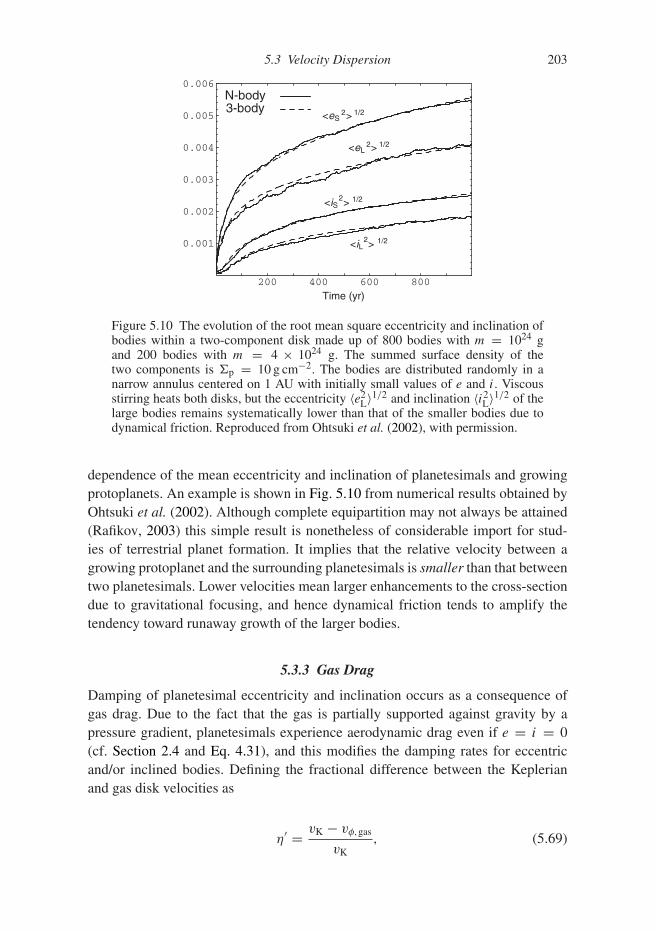
5.3 Velocity Dispersion 203
200 400 600 800
Time (yr)
0.001
0.002
0.003
0.004
0.005
0.006
<e >L2 1/2
<i >L2 1/2
<e >S2 1/2
<i >S2 1/2
N-body3-body
Figure 5.10 The evolution of the root mean square eccentricity and inclination ofbodies within a two-component disk made up of 800 bodies with m = 1024 gand 200 bodies with m = 4 × 1024 g. The summed surface density of thetwo components is �p = 10 g cm−2. The bodies are distributed randomly in anarrow annulus centered on 1 AU with initially small values of e and i. Viscousstirring heats both disks, but the eccentricity 〈e2
L〉1/2 and inclination 〈i2L〉1/2 of the
large bodies remains systematically lower than that of the smaller bodies due todynamical friction. Reproduced from Ohtsuki et al. (2002), with permission.
dependence of the mean eccentricity and inclination of planetesimals and growingprotoplanets. An example is shown in Fig. 5.10 from numerical results obtained byOhtsuki et al. (2002). Although complete equipartition may not always be attained(Rafikov, 2003) this simple result is nonetheless of considerable import for stud-ies of terrestrial planet formation. It implies that the relative velocity between agrowing protoplanet and the surrounding planetesimals is smaller than that betweentwo planetesimals. Lower velocities mean larger enhancements to the cross-sectiondue to gravitational focusing, and hence dynamical friction tends to amplify thetendency toward runaway growth of the larger bodies.
5.3.3 Gas Drag
Damping of planetesimal eccentricity and inclination occurs as a consequence ofgas drag. Due to the fact that the gas is partially supported against gravity by apressure gradient, planetesimals experience aerodynamic drag even if e = i = 0(cf. Section 2.4 and Eq. 4.31), and this modifies the damping rates for eccentricand/or inclined bodies. Defining the fractional difference between the Keplerianand gas disk velocities as
η′ = vK − vφ,gas
vK, (5.69)
204 Terrestrial Planet Formation
Adachi et al. (1976) find that the damping rate of planetesimal eccentricity andinclination can be approximately described via
de
dt= − e
tdrag
(η′2 + 5
8e2 + 1
2i2
)1/2
, (5.70)
di
dt= − i
2tdrag
(η′2 + 5
8e2 + 1
2i2
)1/2
, (5.71)
where the characteristic time scale is defined as
tdrag = 8
3CD
ρms
ρvK. (5.72)
Since η′ is typically a few ×10−3 the term in the parentheses due to the backgroundgas drag is dominant for very small values of e and i, and in this limit the dampingtime scale is independent of the actual values of the eccentricity and inclination.For low eccentricity planetesimals of mass 1019 g and radius 10 km orbiting withina gas disk of density ρ = 5 × 10⁻¹⁰ g cm−3 and η′ = 0.004, for example, thedamping time scale is of the order of 105 yr. This is a long time scale, but as we havenoted it takes progressively longer to excite the random velocities of planetesimalsby viscous stirring as their eccentricities and inclinations increase. It is thereforepossible to reach an equilibrium state in which gas drag is sufficient to maintainthe population of small bodies on almost circular orbits despite the heating due togravitational scattering.
5.3.4 Inelastic Collisions
Sufficiently inelastic collisions between planetesimals can damp eccentricity andinclination by (ultimately) converting some of the random motion into heat withinthe bodies. To estimate the potential importance of this effect we first observe that ifthe gravitational focusing factor is large most “encounters” between planetesimalsresult in gravitational scattering (which is a heating process) rather than physicalcollisions. Inelastic collisions are only potentially significant when σ > vesc, inwhich case the collision time scale is
tinelastic = 1
nswπs2σ. (5.73)
Assuming an isotropic velocity dispersion, the mid-plane number density of plan-etesimals nsw is inversely proportional to σ , which cancels as usual to yield anestimate
tinelastic � 8ρms
3�p�. (5.74)

5.4 Regimes of Planetesimal-Driven Growth 205
We can compare this time scale to the time scale for damping of planetesimalrandom motion by gas drag (Eq. 5.71), which in the limit of small e and i is
tgas � 8ρms
3η′CDρvK. (5.75)
Equating tinelastic to tgas, we find that up to factors of the order of unity the conditionfor inelastic collisions to dominate is
�p>∼ ρrη′. (5.76)
This can be further simplified by noting that the deviation of the gas velocity fromthe Keplerian value η′ ∼ (h/r)2. We find finally
�p
�>∼
h
r, (5.77)
as the condition for inelastic collisions to be more important than gas drag if,additionally, gravitational focusing is unimportant. Since �p/� is assuredly smallerthan the local dust to gas ratio – whose standard value of f = 10−2 is in turn smallerthan the typical (h/r) ≈ 0.05 – this estimate justifies our neglect of inelastic colli-sions relative to aerodynamic drag in the preceding section. One can see, however,that the margin by which inelastic collisions are subdominant is not all that large,and as the gas disk evolves and dissipates it may be possible to encounter a regimein which inelastic collisions provide the main cooling mechanism.
Planetesimal excitation by gravitational coupling to turbulent fluctuations inthe gas disk can also influence the velocity disperson. Many plausible sourcesof disk turbulence (including the magnetorotational instability) create spatialand temporal fluctuations in the gas surface density of the disk. Any solid bodyorbiting within the gas experiences stochastic forcing as a result of the gravitationalforces from the nonaxisymmetric surface density fluctuations, and these randomlydirected impulses act as an excitation mechanism for eccentricity and inclination.For terrestrial planet formation the main interest in this process derives fromthe possibility that excitation due to gravitational coupling to turbulence mightdominate viscous stirring prior to the formation of large protoplanets, and therebydelay or (in some regions of the disk) even prevent collisional growth. Ormeland Okuzumi (2013) provide estimates of the importance of this effect. Sincethe mechanism or mechanisms that result in angular momentum transport withinprotoplanetary disks remain uncertain it will come as no surprise that there remainsubstantial uncertainties.
5.4 Regimes of Planetesimal-Driven Growth
The expressions derived above for the growth rate of protoplanets and for thevelocity evolution of planetesimals are only suitable for order of magnitude

206 Terrestrial Planet Formation
estimates. More accurate semi-analytic formulae can be derived via two approaches:a kinetic formalism that is based on adding a collisional term to the collisionlessBoltzmann equation describing the evolution of the phase-space density of bodies(Hornung et al., 1985; Stewart & Wetherill, 1988), or a celestial mechanics treat-ment of three-body dynamics using Hill’s equations (Ida, 1990). These approachesare equivalent (Stewart & Ida, 2000) and the approximate formulae that resultcan be further improved by reference to numerical integrations of the three-bodyproblem. Inaba et al. (2001), Ohtsuki et al. (2002), and Chambers (2006) providedetailed expressions and fitting formulae that cover much of the parameter regimerelevant for classical planetesimal-driven planet formation models.
Within their domain of validity these semi-analytic formulae for the excitationand damping of planetesimal eccentricity (supplemented where necessary withthe similar expressions for dynamical friction and stirring by planetesimal–planetesimal scattering) are quite accurate. Figures 5.9 and 5.10 show, for example,the comparison between the semi-analytic formulae and N-body results for thecases of one- and two-component disks of bodies evolving under the actionof viscous stirring and dynamical friction, and it is clear that the agreement isimpressively good.
Returning to qualitative considerations, Fig. 5.11 is a sketch of the three possibleregimes that can occur as planetesimals grow into planets. In orderly growth, thetypical mass of bodies increases over time, but the dispersion in mass (in logarith-mic units) does not. In runaway growth, a small number of bodies grow rapidlywhile the bulk of the population of bodies do not. Runaway growth is the normin the early part of classical models of planetesimal-driven terrestrial planet for-mation (Greenberg et al., 1978). At later times, ongoing growth occurs in a highvelocity regime where the planetesimal disk is heated by viscous stirring from the
Orderly growth Runaway growth
Oligarchic growth
Figure 5.11 Illustration of the different regimes of planetesimal-driven growth.
5.5 Coagulation Equation 207
protoplanets and cooled by gas drag (Ida & Makino, 1993). This regime, known asoligarchic growth, is partially self-limiting, since growth of any individual proto-planet increases the random velocities of planetesimals in its vicinity and decreasesthe gravitational focusing enhancement to the collision cross-section.
Although these regimes were originally defined in the context of models whereplanetesimals provided the only mechanism of growth, the same classification isuseful in more general models that include the possibility of pebble accretion.
5.5 Coagulation Equation
For much of the preceding discussion we have assumed that the distribution ofmasses of the growing bodies can be partitioned into two groups: large planetaryembryos with mass M and negligible random velocities, and much less massiveplanetesimals with mass m and significant random velocities. If runaway growthoccurs this simple approximation is actually quite a good way to think about theproblem, since each annulus of the disk will contain one body that is much largerthan all the rest. One may rightly worry, however, that attempting to demonstratethe existence of runaway growth using a two-groups approximation involves asuspiciously circular logic. The right framework for approaching the problem ofwhether runaway growth occurs requires dropping the two-groups model and treat-ing the evolution of an arbitrary size distribution of bodies using the methods ofcoagulation theory (Smoluchowski, 1916). The application of this theory to planetformation was pioneered by Safronov (1969), and has subsequently been adoptedby many authors. Clear descriptions of the basic method are given by Wether-ill (1990) and Kenyon and Luu (1998), whose nomenclature is largely adopted here.
Coagulation theory is based on solutions to the coagulation equation, which canbe written equivalently in either integral (Eq. 4.74) or discrete form. In the discreterepresentation, we assume that at some time t there are nk bodies within some fixedvolume that have a mass km1 that is an integral multiple of some small mass m1.We treat nk as a continuous function.4 Ignoring radial migration and fragmentation,we can then write the discrete coagulation equation for an annulus of the disk in theform
dnk
dt= 1
2
∑i+j=k
Aijninj − nk
∞∑i=1
Aikni, (5.78)
where the Aij , known as the kernels, describe the probability of a collision that leadsto accretion between bodies with masses im1 and jm1 per unit time. In generalthese will be nonlinear functions of the masses, random velocities, and physicalproperties (e.g. density) of the bodies involved. One observes that the number of
4 This is reasonable provided that nk � 1, but we must be cognizant that the statistical foundations of themethod can break down if for some k of interest nk ∼ 1.

208 Terrestrial Planet Formation
bodies in the kth mass bin changes due to two processes. First, the number of bodiesof mass km1 increases whenever there is a collision between any pair of bodieswhose total mass (i+j)m1 sums to km1 (the factor of 1/2 is present to avoid doublecounting these collisions). Second, the number of bodies of mass km1 decreaseswhenever there is any collision with a body of any other mass.
There are no known analytic solutions to the coagulation equation for kernelsthat encode the critical physics of planet formation – gravitational focusing andmass-dependent velocity dispersion. Numerical solutions provide the only way tohandle these complexities. We can, however, gain some insight into the nature ofgeneral solutions to the coagulation equation by studying three known solutions forcases with particularly simple kernels. If
Aij = α, (5.79)
where α is a constant, and there are initially n0 bodies with mass m1, then at time t
nk = n0f2(1 − f )k−1, (5.80)
f = 1
1 + 12αn0t
. (5.81)
Inspection of the units shows that f is a dimensionless measure of the time. Thephysical interpretation of f is that it is the fraction of bodies in the smallest massbin that have yet to collide with any other body.
The solution expressed in Eq. (5.81) is plotted in Fig. 5.12. This solution is anexample of orderly growth. As time progresses the mean mass of the populationincreases, but the shape of the mass spectrum approaches an asymptotic form andits width (expressed in logarithmic units) does not increase. Qualitatively similar isthe solution for the kernel
Aij = α(mi + mj), (5.82)
which has the form
nk = n0kk−1
k!f (1 − f )k−1 exp[−k(1 − f )], (5.83)
f = exp[−αn0t]. (5.84)
This solution also exhibits orderly growth.The final known solution applies to the case of a kernel that is the product of the
masses of the bodies,
Aij = αmimj . (5.85)
In this case,
nk = n0(2k)k−1
k! k
(1
2αn0t
)k−1
exp[−αn0kt]. (5.86)

5.5 Coagulation Equation 209
Figure 5.12 Solution to the coagulation equation for the simple case in whichthe kernel Aij = α is a constant. Initially all bodies have mass m1. The solutionis plotted for scaled times t ′ ≡ αn0t equal to 1, 10, 100, and 103. The upperpanel shows the evolution (on an arbitrary vertical scale) of the number of bodiesnk as a function of mass, while the lower panel shows the evolution of the massdistribution.
This solution is plotted in Fig. 5.13 together with a solution for the case of aconstant kernel that has the same initial collision rate. Equation (5.86) representsa qualitatively different class of solution to the coagulation equation, in whichrunaway growth develops. The mass distribution develops a power-law tail towardhigh masses as a small number of bodies grow rapidly at the expense of all of theothers. Solutions to the coagulation equation that display runaway growth generallyapply only at early times, since once most of the mass accumulates into a singlemassive body the assumptions upon which the coagulation equation is based breakdown. Formally Eq. (5.86) is valid up until a time αn0t = 1.
Realistic kernels for planet formation do not scale with mass in the same wayas any of the analytically tractable forms. If gravitational focusing is unimportant,the collision cross-section scales with the geometric area and A ∝ R2
s ∝ m2/3.This scaling is bracketed by the two analytic solutions that display orderly growth.Conversely, if gravitational focusing dominates then A ∝ mRs ∝ m4/3, which liesbetween analytic solutions exhibiting orderly and runaway growth. This observa-tion does not allow us to draw any definitive conclusions, but numerical calculations

210 Terrestrial Planet Formation
Figure 5.13 Comparison of the analytic solution to the coagulation equation withthe kernel Aij = α (dashed lines) to that with Aij = αmimj (solid lines). Thesolutions are plotted for scaled times t ′ ≡ αn0t equal to 10−3, 10−2, 0.1, and 1.The collision rate for i = j = 1 is identical for the two solutions, so the veryearly time behavior is the same. Large differences develop just prior to the onsetof runaway growth at a time αn0t = 1.
suggest that runaway growth can occur for kernels that describe collisions duringthe early phases of planet formation.
5.6 Pebble Accretion
The “classical” model of planet formation, in which growth occurs due to collisionsbetween and among protoplanets and planetesimals, is the only possibility if theplanetesimal formation process efficiently removes all (or almost all) small solidparticles from the disk. Observationally, this is not what appears to happen. Dustand mm-sized grains are present in protoplanetary disks during all evolutionaryphases, including at late times when planetesimals and larger bodies are very likelyto have formed. This fact motivates us to consider how a growing planet wouldinteract with solid bodies of arbitrary sizes during the period when gas is stillpresent within the disk.
Figure 5.14 illustrates some of the main possibilities. The upper panels depictpossible flows for bodies whose gravity is weak (think, for example, of a km-scaleplanetesimal). Very small dust particles, which are tightly coupled to the gas viaaerodynamic forces, simply flow around the body. Larger objects, which experiencenegligible aerodynamic forces, collide and accrete only if their trajectories at largedistance intersect the geometric cross-section of the body.
The lower panels of the figure illustrate what can happen for larger bodies whosegravity can significantly deflect the trajectories of passing objects. This leads toaccretion cross-sections that exceed the geometric one. We have already discussed

5.6 Pebble Accretion 211
r
φ
r
φ
r
φ
r
Geometric accretion Entrained flow
Aerodynamically assisted pebble accretion
Planetesimal accretion
Hill sphere
Gas-free and / or planetesimal limit
Aerodnamicallycoupled solidswithin gas
Extremely smallsolid particles
Boo
sted
acc
retio
ncr
oss-
sect
ion
Acc
retin
gtra
ject
orie
s
Nonaccretingtrajectories
Nonaccretingtrajectories
Large particlesand weak gravity
Hill sphere
φ
Figure 5.14 Illustration of some of the regimes of interaction between a growingplanet and solid particles or larger planetesimals (after Ormel 2017). For relativelylarge bodies, the cross-section for the aerodynamically assisted accretion ofparticles (lower left panel) can be much larger than for planetesimals (lower rightpanel).
the enhancement due to gravitational focusing, which is relevant for planetesimalsinteracting with growing planets in a regime that is effectively gas-free. The cross-section is also boosted for solid particles whose size is such that they experiencesignificant gravitational and aerodynamic forces during their encounter. This is theregime of aerodynamically assisted or pebble accretion (Ormel & Klahr, 2010;Lambrechts & Johansen, 2012). Pebble accretion is a qualitatively distinct growthmechanism for planets. Instead of depending upon the local density and velocitydispersion of planetesimals, as is the case for planetesimal-driven growth, the keyfactors are the local density and dimensionless friction time of small solid particles.Pebble accretion can be more efficient than planetesimal accretion, and its depen-dence on different factors allows for growth in a broader range of circumstances.
In this section we discuss the key physics of pebble accretion. Before doing so, anote on nomenclature is appropriate. For most of us, the word “pebble” conjures upan image of stones with sizes similar to those found, for example, on beaches. Thereis also a formal geological definition of pebbles as particles with sizes between
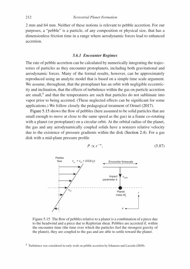
212 Terrestrial Planet Formation
2 mm and 64 mm. Neither of these notions is relevant to pebble accretion. For ourpurposes, a “pebble” is a particle, of any composition or physical size, that has adimensionless friction time in a range where aerodynamic forces lead to enhancedaccretion.
5.6.1 Encounter Regimes
The rate of pebble accretion can be calculated by numerically integrating the trajec-tories of particles as they encounter protoplanets, including both gravitational andaerodynamic forces. Many of the formal results, however, can be approximatelyreproduced using an analytic model that is based on a simple time scale argument.We assume, throughout, that the protoplanet has an orbit with negligible eccentric-ity and inclination, that the effects of turbulence within the gas on particle accretionare small,5 and that the temperatures are such that particles do not sublimate intovapor prior to being accreted. (These neglected effects can be significant for someapplications.) We follow closely the pedagogical treatment of Ormel (2017).
Figure 5.15 shows the flow of pebbles (here assumed to be solid particles that aresmall enough to move at close to the same speed as the gas) in a frame co-rotatingwith a planet (or protoplanet) on a circular orbit. At the orbital radius of the planet,the gas and any aerodynamically coupled solids have a nonzero relative velocitydue to the existence of pressure gradients within the disk (Section 2.4). For a gasdisk with a mid-plane pressure profile
P ∝ r−n, (5.87)
f
v∞ = vhw + (3/2)WKb Encounter timescale
Impactparameter b
vsettle
vhw
Pebbleflow
rPlanet mass Mp
Figure 5.15 The flow of pebbles relative to a planet is a combination of a piece dueto the headwind and a piece due to Keplerian shear. Pebbles are accreted if, withinthe encounter time (the time over which the particles feel the strongest gravity ofthe planet), they are coupled to the gas and are able to settle toward the planet.
5 Turbulence was considered in early work on pebble accretion by Johansen and Lacerda (2010).

5.6 Pebble Accretion 213
the resulting headwind velocity is
vhw = 1
2n
(h
r
)2
vK, (5.88)
where (h/r) is the geometric thickness of the disk and vK = √GM∗/r is the
Keplerian orbital speed. Numerically
vhw = 35(n
3
)(h/r
0.05
)2 (M∗M�
)1/2 ( r
10 AU
)−1/2m s−1. (5.89)
This is the speed with which a pebble, moving with the gas at the same orbitalradius as the planet, would approach the planet.
The headwind speed depends upon the disk structure. For a disk with a power-law surface density profile and a mid-plane temperature profile, Tc ∝ r−1/2, n is aconstant and (h/r) ∝ r1/4. In this special case the radial dependence arising from(h/r) and vK cancels out in the above equation, and vhw is just a constant throughoutthe disk.
Pebbles that encounter the planet with non-co-orbital trajectories do so with arelative velocity at large distance v∞ that is the sum of the headwind speed anda piece due to Keplerian orbital shear. For a pebble with an impact parameter b asimple calculation gives
v∞ = vhw + 3
2�Kb. (5.90)
If v∞ is dominated by the first term on the right-hand-side, we say the encounteris in the headwind regime (also called the “Bondi” regime by some authors).Otherwise, the encounter is in the shear (or “Hill”) regime. The dividing linebetween these regimes occurs for an impact parameter b = (2/3)vhw�−1
K .
5.6.2 Pebble Accretion Conditions
Whether a pebble encountering a planet will be accreted can be estimated by con-sidering the ordering of three time scales. We have already defined (in Section 4.2)the friction (or stopping) time scale tfric, along with its dimensionless versionτfric = tfric�K. In the Epstein drag regime the friction time is velocity independent,
tfric = ρm
ρ
s
vth, (5.91)
and depends only on the particle size s, the particle material density ρm, the gasdensity ρ, and the gas thermal speed vth.
The encounter with the planet introduces two new time scales. The first is theencounter time scale
tenc = 2b
v∞, (5.92)
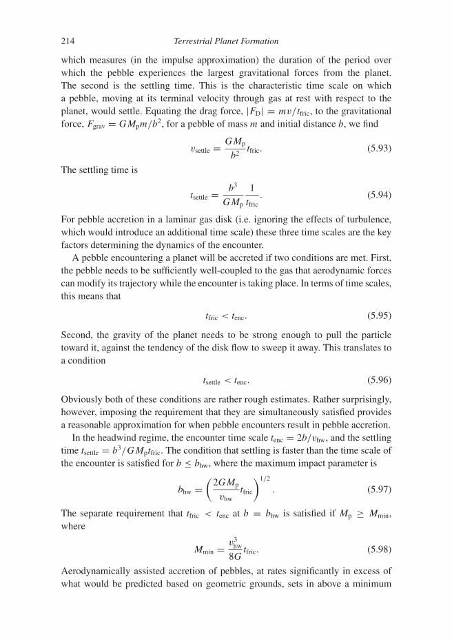
214 Terrestrial Planet Formation
which measures (in the impulse approximation) the duration of the period overwhich the pebble experiences the largest gravitational forces from the planet.The second is the settling time. This is the characteristic time scale on whicha pebble, moving at its terminal velocity through gas at rest with respect to theplanet, would settle. Equating the drag force, |FD| = mv/tfric, to the gravitationalforce, Fgrav = GMpm/b2, for a pebble of mass m and initial distance b, we find
vsettle = GMp
b2tfric. (5.93)
The settling time is
tsettle = b3
GMp
1
tfric. (5.94)
For pebble accretion in a laminar gas disk (i.e. ignoring the effects of turbulence,which would introduce an additional time scale) these three time scales are the keyfactors determining the dynamics of the encounter.
A pebble encountering a planet will be accreted if two conditions are met. First,the pebble needs to be sufficiently well-coupled to the gas that aerodynamic forcescan modify its trajectory while the encounter is taking place. In terms of time scales,this means that
tfric < tenc. (5.95)
Second, the gravity of the planet needs to be strong enough to pull the particletoward it, against the tendency of the disk flow to sweep it away. This translates toa condition
tsettle < tenc. (5.96)
Obviously both of these conditions are rather rough estimates. Rather surprisingly,however, imposing the requirement that they are simultaneously satisfied providesa reasonable approximation for when pebble encounters result in pebble accretion.
In the headwind regime, the encounter time scale tenc = 2b/vhw, and the settlingtime tsettle = b3/GMptfric. The condition that settling is faster than the time scale ofthe encounter is satisfied for b ≤ bhw, where the maximum impact parameter is
bhw =(
2GMp
vhwtfric
)1/2
. (5.97)
The separate requirement that tfric < tenc at b = bhw is satisfied if Mp ≥ Mmin,where
Mmin = v3hw
8Gtfric. (5.98)
Aerodynamically assisted accretion of pebbles, at rates significantly in excess ofwhat would be predicted based on geometric grounds, sets in above a minimum

5.6 Pebble Accretion 215
mass that is linearly proportional to the stopping time (and hence to the particlesize, in the Epstein regime).
In the shear regime, the encounter velocity v∞ � (3/2)�Kb. The encounter timescale, tenc = 2b/v∞, is then
tenc ≈ �−1K . (5.99)
The form of the encounter time scale in the shear regime guarantees that the con-dition that tfric < tenc is satisfied for all particles with τfric
<∼ 1. Equating tsettle withtenc, we find that the maximum impact parameter for pebble accretion is
bsh =(
GMp
�Ktfric
)1/3
. (5.100)
The maximum impact parameter scales more weakly with planet mass in the shearregime as compared to the headwind regime. The transition between the regimesoccurs at a critical mass Mcrit, which can be found by setting bhw = bsh. The result is
Mcrit = 1
8
Mt
τfric, (5.101)
which we have written in this way to emphasize that the transition depends uponboth the planet mass and the pebble size, defined in terms of its dimensionlessstopping time. The characteristic mass Mt depends only on the headwind speed andon the angular velocity,
Mt ≡ v3hw
G�K. (5.102)
The headwind regime is valid for low planet masses, while the shear regime appliesfor Mp > Mcrit.
Unless τfric is very small the shear regime of pebble accretion is appropriate forall except the lowest protoplanet masses. Using the expression for vhw (Eq. 5.88)the characteristic mass is
Mt = 1
8n3
(h
r
)6
M∗. (5.103)
The strong dependence on the disk thickness means that Mt is an increasing func-tion of orbital radius (scaling as r3/2 for simple irradiated disk models). Takingn = 3 and M∗ = M�, we obtain Mt = 2.4 × 10⁻⁴ M⊕ for (h/r) = 0.03 andMt = 5.2 × 10⁻³ M⊕ for (h/r) = 0.05.
The potential importance of pebble accretion as a mechanism for planetarygrowth can be grasped by rewriting the maximum impact parameter for accretionin the shear regime (Eq. 5.100) in a different, but equivalent, form:
bsh =(
GMp
�Ktfric
)1/3
=(
GMp
�2K
)1/3
τ1/3fric ≈ τ
1/3fric rH, (5.104)

216 Terrestrial Planet Formation
where rH is the Hill radius of the planet. For particles with τfric ∼ 1 the cross-section for pebble accretion can be as large as the entire Hill sphere of the accretingplanet. This is a very large cross-section indeed. Suppose we have a planet at orbitalradius a with mass Mp, radius Rs, and density ρm. Comparing the geometric cross-section πR2
s to the maximum pebble accretion cross-section πr2H gives a “pebble
enhancement factor” that is loosely analogous to the gravitational focusing factorfor planetesimal accretion. The maximum pebble enhancement factor is
Fpebble = r2H
R2s
=(
4πρm
9M∗
)2/3
a2. (5.105)
Taking ρm = 1 g cm−3 and M∗ = M⊕,
Fpebble ∼ 2 × 10⁴( a
AU
)2. (5.106)
At large orbital radii, especially, the peak cross-section for a planet to sweep uppebbles is very large. Realizing this theoretical limit requires, of course, that thepebbles in the vicinity of the planet have close to the optimal size, and obtaining alarge accretion rate additionally requires a large enough density in pebbles. Becauseof these caveats, detailed models are needed to determine whether the pebble accre-tion rate exceeds that of planetesimal accretion for a given situation.
5.6.3 Pebble Accretion Rates
If the pebbles form a layer whose thickness exceeds the maximum impact parameterof the planet, the pebble accretion rate is simply
Mp = πb2v∞ρpebble, (5.107)
where ρpebble is the volume density of pebbles encountering the planet. Substitutingfor the impact parameter one finds
Mp ≈ 2πGMptfricρpebbles, (5.108)
which is valid in both the headwind and shear regimes of pebble accretion.If, instead, the pebbles occupy a very thin layer with surface density �pebble,the accretion rate is given by Mp = 2bv∞�pebble. Across the different regimes thescaling of the accretion rate with planet mass is at most linear. Accordingly, pebbleaccretion does not facilitate runaway growth.
5.6.4 Relative Importance of Pebble Accretion
There is no simple answer to the question of when pebble accretion dominates overplanetesimal accretion. Among other factors, the balance depends upon:
5.7 Final Assembly 217
• The size distribution of aerodynamically-relevant solids, and the gas disk struc-ture, which together determine tfric.
• The fraction of the total solid mass that forms planetesimals, rather than remain-ing in the pebble size range.
• The time-dependent drift of pebbles radially through the disk, and the extent towhich protoplanets at larger radii (than the one being considered) sweep themup first.
• The thickness of the pebble layer, which will be set by turbulent stirring. (Notethat we have ignored turbulence in our discussion, but that this is another relevantparameter.)
• The full suite of processes that determine the gravitational focusing factor forplanetesimals.
The accretion of pebbles can be a self-limiting process. As the planet grows inmass, the surface density profile of the gas in the vicinity is modified by angularmomentum exchange mediated by gravitational torques. If this leads to the forma-tion of a local pressure maximum upstream of the planet, radial drift of pebblestoward the planet will be halted (see Section 4.3.2). This occurs at the pebbleisolation mass, which has been estimated to be (Morbidelli & Nesvorny, 2012;Ormel, 2017)
Mp,pebble−iso ∼ 40M⊕
(h/r
0.05
)3
. (5.109)
Pebble isolation is closely related to the process of gap opening (discussed inChapter 7), and it likewise involves complex and not fully understood aspectsof disk physics. However, on order of magnitude grounds, it can clearly bean important phenomenon as planet masses approach those where runaway gasaccretion occurs in core accretion models of giant planet formation.
5.7 Final Assembly
A fiducial model for the formation of terrestrial planets with properties (massesand orbital radii) similar to those in the Solar System, based on planetesimal-drivenaccretion only, can be developed based on the aforementioned physics. Startingfrom a large population of planetesimals the first two phases are:
• Runaway growth. Initially there are no large bodies, so the random velocity ofplanetesimals is set by a balance between viscous stirring among the planetesi-mals themselves and damping via gas drag. The combined influence of dynamicalfriction and gravitational focusing results in runaway growth of a small fractionof planetesimals.
• Oligarchic growth. Runaway growth ceases at the point when the rate of vis-cous stirring of the planetesimals by the largest bodies first exceeds the rate

218 Terrestrial Planet Formation
of self-stirring among the planetesimals. The resulting boost in the strength ofviscous stirring increases the equilibrium values of planetesimal eccentricity andinclination, partially limiting the gravitationally enhanced cross-section of theprotoplanets. In this regime the growth of protoplanets continues to outrun thatof planetesimals, but the dominance is local rather than global. Across the diskmany oligarchs grow at similar rates by consuming planetesimals within theirown largely independent feeding zones.
These initial stages of terrestrial planet formation are rapid (of the order of0.01–1 Myr), and result in the formation of perhaps 102 to 103 large bodies acrossthe terrestrial planet zone. These are massive objects (of the order of 10−2 M⊕ to0.1 M⊕, so comparable to the mass of the Moon or Mercury) but they are not yetterrestrial planets.
The final assembly of terrestrial planets gets underway once the oligarchs havedepleted the planetesimal disk to the point that dynamical friction can no longer
Semi-major axis (AU) Semi-major axis (AU)Log (water mass fraction)
Figure 5.16 Results from a high resolution simulation of the final assembly ofterrestrial planets (Raymond et al., 2006). The initial conditions for this simulationare representative of the late stages of oligarchic growth, with approximately 2000planetary embryos (shaded according to their water content) distributed in a diskwith a surface density profile of �p ∝ r−3/2 and a surface density at 1 AU of10 g cm−2. Jupiter is assumed to have a circular orbit at 5.5 AU during the durationof the final assembly phase, which takes around 100 Myr. Reproduced in modifiedform from Raymond et al. (2006), with permission.

5.8 Further Reading 219
maintain low eccentricities and inclinations of the oligarchs. Beyond this pointthe assumption that each oligarch grows in isolation breaks down, and the largestbodies start to interact strongly, collide, and scatter smaller bodies across a signif-icant radial extent of the disk. Numerical N-body simulations (examples includeRaymond et al., 2006 and O’Brien et al., 2006), an example of which is shownin Fig. 5.16, show that this final stage is by far the slowest, with large collisionscontinuing out to at least tens of Myr. The process is chaotic, and hence identicalinitial conditions can give rise to a range of outcomes that must be compared tothe observed properties of the Solar System’s terrestrial planets statistically. Thelevel of agreement attained is by no means perfect, with the small mass of Mars(compared to that of the Earth and Venus) being the most important discrepancy.Viewed on a coarser level, however, reasonable values of the disk surface densityin the inner Solar System do appear roughly to reproduce the observed propertiesof the terrestrial planets.
It is possible to extend the fiducial model for Solar System terrestrial planet for-mation, and consider how modest changes in the input parameters would affect thelikely outcome. For example, both elementary stability arguments and numericalsimulations predict that there ought to be a dependence on the surface density ofthe planetesimal disk, in the sense that higher �p typically yields a smaller numberof more massive planets (Wetherill, 1996; Kokubo et al., 2006). This type of extrap-olation has its limits, however, and when considering planets around solar-type starsin closer orbits, or habitable planets around lower-mass stars, qualitatively differentformation histories may be involved. A significant role for pebble accretion is onepossibility. Another is that migration may play a dominant role in determining thefinal architecture.
5.8 Further Reading
“Planet Formation by Coagulation: A focus on Uranus and Neptune,” P. Goldreich,Y. Lithwick, & R. Sari (2004), Annual Review of Astronomy & Astrophysics, 42,549. This review includes useful “back of the envelope” estimates of planetary growthmechanisms.
“The Emerging Paradigm of Pebble Accretion,” C. W. Ormel (2017), in Formation, Evolu-tion, and Dynamics of Young Solar Systems, Astrophysics and Space Science Library,445, Cham: Springer, p. 197.
“Terrestrial Planet Formation at Home and Abroad,” S. N. Raymond, et al. 2014, in Proto-stars and Planets VI, H. Beuther, R. S. Klessen, C. P. Dullemond, & T. Henning (eds.),Tucson: University of Arizona Press, p. 595.

6
Giant Planet Formation
Planets with masses above a few times the mass of the Earth typically have radiithat are large enough to indicate the presence of a substantial gaseous envelope.In the Solar System the gas giants, Jupiter and Saturn, and the ice giants, Uranusand Neptune, fall into this class, with properties quite different from the terrestrialplanets. In extrasolar planetary systems the masses of apparently rocky worldsappear to overlap with those of planets that have significant envelopes, but thereis still a rough threshold mass above which envelopes are the norm.
The formation of giant planets within the core accretion model is understood asan extension of the processes that form terrestrial planets. A “core” of rocky and/oricy material grows, via a combination of pebble and planetesimal accretion, to amass large enough to capture a significant gaseous envelope before the gas disk isdispersed. Initially the envelope is less massive than the core, and if the gas diskis dispersed while this is still the case the result is a planet qualitatively similar toa Solar System ice giant or an extrasolar mini-Neptune. If, instead, the envelopegrows to become comparable in mass to the core, a phase of rapid gas accretionstarts and the result is a fully formed gas giant. The time scale for giant planetformation in this model hinges on how quickly the core is assembled and on howrapidly the gas in the envelope can cool and accrete on to the core.
The goal in this chapter is to describe the physical principles behind core accre-tion and to provide a summary of some of the relevant observational constraints. Wealso discuss the conditions under which the gas disk can become gravitationallyunstable and fragment into bound objects. Historically, gravitationally instabilitywas studied primarily as an alternative mechanism for forming giant planets. Morerecent work suggests that the masses of objects formed as a result of gravitationalinstability would normally exceed those of most planets, but the process is still ofinterest as a way of rapidly forming substellar objects (including, perhaps, someplanetary mass objects) at large orbital radii.
220

6.1 Core Accretion 221
6.1 Core Accretion
The core accretion model for gas giant formation rests on one assumption: thata seed planet or core grows via pebble accretion or two-body collisions rapidlyenough that it can exceed a certain critical mass prior to the dissipation of thegas disk. If this condition is satisfied, it can be shown (Perri & Cameron, 1974;Mizuno, 1980) that the core triggers a hydrodynamic instability that results in theonset of rapid gas accretion on to the core. Since the critical core mass is typicallyof the order of 5–10 M⊕, the end result is a largely gaseous but heavy elementenriched planet that at least qualitatively resembles Jupiter or Saturn.
Figure 6.1 illustrates the four main phases in the formation of giant planets viacore accretion:
• Core formation. A solid protoplanet (which henceforth we will rename a“core”) grows via a combination of pebble accretion and planetesimal collisions
(1) Mcore >> Menv
(2) Mcore > Menv
(3) Mcore ~ Menv
(4) Mcore << Menv
Pebble accretion
Planetesimalaccretion Core formation
within gas disk
Accretion of gas envelope
Core exceeds the critical mass
Rapid envelope accretion phase
Gas disk dispersal
Kelvin–Helmholtzcontraction
Mixing of core material intoenvelope
Figure 6.1 Stages in the formation of giant planets via core accretion.
222 Giant Planet Formation
until it becomes massive enough to retain a significant gaseous atmosphere orenvelope. The physics during this initial phase is identical to that discussedin the context of terrestrial planet formation in Chapter 5, with the rate ofgrowth being controlled by the aerodynamics of small solid bodies, the initialsurface density of rocky and icy planetesimals, and by the extent of gravitationalfocusing.
• Hydrostatic growth. Initially the envelope surrounding the solid core is in hydro-static equilibrium. Energy liberated by planetesimals impacting the core, togetherwith gravitational potential energy released as the envelope itself contracts, mustbe transported through the envelope by radiative diffusion or convection beforeit is lost to the large gas reservoir of the protoplanetary disk. Over time boththe core and the envelope grow until eventually the core exceeds a critical mass.The critical mass is not a constant but rather a calculable function of (primarily)the planetesimal accretion rate and opacity in the envelope.
• Runaway growth. Once the critical mass is exceeded a runaway phase of gasaccretion ensues. The rate of growth is no longer demand limited (defined by thecooling properties of the envelope) but instead supply limited and defined by thehydrodynamic interaction between the growing planet and the disk. For massiveplanets the bulk of the planetary envelope is accreted during this phase, which istypically rather brief – of the order of 105 yr.
• Termination of accretion. Eventually the supply of gas is exhausted, eitherbecause of the dissipation of the entire protoplanetary disk or as a consequence ofthe planet opening up a local gap in the disk (the physics of gap opening will bediscussed more fully in Chapter 7). Accretion tails off and the planet commencesa long phase of cooling and quasi-hydrostatic contraction. If the core material issoluble in the surrounding envelope, some fraction of the primordial core maydissolve into the gas to form a fuzzy structure with a dense inner core and a diluteouter core.
We can readily estimate some of the masses that characterize the transitionsbetween these phases. The weakest condition that must be satisfied if a planetembedded within a gas disk is to hold on to a bound atmosphere is that the escapespeed vesc at the surface of the planet exceeds the sound speed cs within the gas.1
A solid body of mass Mp and material density ρm has a radius
Rs =(
3
4π
Mp
ρm
)1/3
, (6.1)
1 A planet that marginally satisfies this condition would lose its atmosphere on approximately the dynamicaltime scale in the absence of the gas disk, so this is not the same condition as for an isolated planet to be ableto retain an atmosphere. To avoid atmospheric erosion via the process known as Jeans escape, an isolatedplanet must have a much higher surface escape speed that suffices to retain molecules far out in theMaxwellian tail of the particle velocity distribution.

6.1 Core Accretion 223
and a surface escape speed
vesc =√
2GMp
Rs. (6.2)
Noting that the sound speed in the protoplanetary disk can be written in terms ofthe disk thickness (h/r) and Keplerian velocity vK via
cs =(
h
r
)vK, (6.3)
the condition that vesc > cs can be expressed as
Mp >
(3
32π
)1/2 (h
r
)3M
3/2∗
ρ1/2m a3/2
, (6.4)
where a is the orbital radius. This mass is very small. Substituting numbers appro-priate for an icy body at 5 AU in a disk around a solar mass star with (h/r) = 0.05we find that some atmosphere will be present provided that Mp
>∼ 5 × 10⁻⁴ M⊕.The existence of a tenuous wisp of an atmosphere will not have any dynamical
importance. A more pertinent question is what is the minimum core mass able tomaintain an envelope with a mass that is a non-negligible fraction of the mass ofthe core? To estimate this mass we assume that the envelope makes up a smallfraction ε of the total planet mass, in which case the equation expressing hydrostaticequilibrium for the envelope can be written as
dP
dr= −GMp
r2ρ, (6.5)
where r is the distance from the center of the planet and Mp can be consideredto be a constant. To keep the problem simple (this is after all only an estimate)we also assume that the envelope is isothermal, so that the pressure P = ρc2
s .Equation (6.5) can then be integrated immediately to yield an expression for theradial density profile of the gas in the envelope:
ln ρ = GMp
c2s
1
r+ const. (6.6)
The constant of integration on the right-hand-side can be evaluated by matching theenvelope density ρ to the density ρ0 in the unperturbed disk at the radius rout, wherethe escape velocity from the planet matches the disk sound speed,
rout = 2GMp
c2s
. (6.7)
With the constant thereby determined, the envelope density profile is
ρ(r) = ρ0 exp
[GMp
c2s
1
r− 1
2
]. (6.8)
224 Giant Planet Formation
The density at the disk mid-plane ρ0 can itself be written in terms of the surfacedensity � and vertical scale-height h as ρ0 = (1/
√2π)(�/h) (Eq. 2.19).
Most of the mass of an envelope with the above density profile lies in a shellclose to the surface of the solid core. We can therefore approximate the envelopemass as
Menv ≈ 4
3πR3
s ρ(Rs), (6.9)
where ρ(Rs) is the envelope density evaluated at the surface of the core. Substitut-ing for both the density profile and Rs, the condition that the envelope makes up anon-negligible fraction of the total mass,
Menv > εMp, (6.10)
reduces to
Mp>∼
(3
4πρm
)1/2 (c2
s
G
)3/2 [ln
(ερm
ρ0
)]3/2
. (6.11)
The dominant dependence is on the disk sound speed, which is a decreasing func-tion of radius. A growing protoplanet will therefore start to acquire a substantialgaseous envelope at a lower mass if it is located in the cool outer regions of the disk.To give a concrete example, we consider an icy body (ρm = 1 g cm−3) growing at5 AU in a disk with ρ0 = 2 × 10⁻¹¹ g cm−3 and sound speed cs = 7 × 104 cm s−1.Taking ε = 0.1 to represent the threshold above which the envelope could be saidto be significant, we predict that this will occur for planet masses
Mp>∼ 0.2 M⊕. (6.12)
At 1 AU, on the other hand, where the disk parameters might be a density ρ0 = 6 ×10⁻¹⁰ g cm−3 and a sound speed cs = 1.5 × 105 cm s−1, a rocky protoplanet (ρm =3 g cm−3) must grow to Mp ∼ M⊕ before we would expect to find it enshrouded ina dense massive envelope.
In light of the rather crude analysis that we have employed, Eq. (6.11) shouldonly be trusted to an order of magnitude. Taking the estimate at face value, however,we can motivate the classical argument for why the Solar System’s gas giant planetsformed only in the cool outer regions of the protoplanetary disk. As we have seen,a protoplanet must grow to something like the mass specified in Eq. (6.11) beforeit starts to acquire a massive gaseous envelope, and this must occur prior to thedispersal of the protoplanetary disk. If we assume that the maximum protoplanetmass that can be attained prior to disk dispersal is comparable to the isolation mass(Eq. 5.53), we can determine for any particular disk model where in the disk planetswill grow fast enough to capture envelopes. As an example, let us suppose that theradial profiles of the gas surface density and solid surface density are those specifiedby the minimum mass Solar Nebula model given in Section 1.2, and that the sound

6.1 Core Accretion 225
Figure 6.2 The radial dependence of the isolation mass (dashed curve) ascompared to the minimum planet mass needed to sustain a massive envelope(solid curve). Both curves are computed for a solar mass star surrounded by adisk with (h/r) = 0.05. The surface density of the gas and solid component istaken to follow Hayashi’s minimum mass Solar Nebula model, with a snow lineat 2.7 AU. In computing the minimum mass necessary for envelope capture it hasbeen assumed that interior to the snow line ρm = 3 g cm−3, while beyond the snowline ρm = 1 g cm−3.
speed is that appropriate to a disk with a constant geometric thickness (h/r) =0.05.2 Equations (5.53) and (6.11) then yield estimates for the isolation mass andthe minimum mass necessary for envelope capture, and these estimates are plottedin Fig. 6.2. The result is suggestive. Interior to the snow line the isolation mass issmaller than the minimum mass required for envelope capture. In this region it isunlikely that protoplanets will grow fast enough to capture envelopes prior to diskdispersal, and the ultimate outcome of planet formation will instead be terrestrialplanets. At orbital radii beyond the snow line, conversely, the isolation mass exceedsthe minimum envelope capture mass. Giant planet formation is much more probablein this case, though as yet we cannot say whether the outcome is planets with amodest but still significant envelope (akin to Uranus and Neptune) or true gas giantswhose mass is dominated by the contribution from the envelope.
It is fair to assume that in a counterfactual world, where the properties of extra-solar planetary systems were known but those of the Solar System were not, theabove argument would never have surfaced. We now know that a large fractionof stars have planets with significant gas content that orbit within 1 AU, contraryto the prediction of the simple model. The basic factors that determine whetherplanets end up as rocky or gaseous worlds, however, remain valid. Rocky planetsare the result if growth, whether from planetesimal or pebble accretion, is too slow,
2 This value is adopted for consistency with most of the other estimates given in this section. It is not strictlyconsistent with the temperature profile usually assumed for the minimum mass Solar Nebula.

226 Giant Planet Formation
and there is a radial dependence to the ease with which a planet can capture anenvelope and proceed to the runaway phase of accretion.
6.1.1 Core/Envelope Structure
The physical underpinning of the core accretion model for gas giant planet for-mation is the existence of a critical core mass – a core mass beyond which itis not possible to find a hydrostatic solution for the structure of a surroundinggaseous envelope. To understand the origin of the critical core mass, we modifysome standard results from the theory of stellar structure to describe the structureof a giant planet envelope. We assume that the planet of total mass Mp has a well-defined solid core of mass Mcore and an envelope mass Menv. Rotation is neglectedand the envelope is taken to be in hydrostatic and thermal equilibrium. Conservationof mass and momentum then yield two differential equations for the structure of theenvelope:
dM
dr= 4πr2ρ,
dP
dr= −GM
r2ρ.
(6.13)
Here P is the pressure and M = M(r) is the total mass enclosed within radius r .We have now dropped the simplifying assumption that M � Mcore so the aboveequations are valid regardless of the mass of the envelope.
Although these equations only involve P and ρ, the temperature invariably entersas a third variable because the pressure P = P(ρ,T ) depends upon it. The temper-ature is determined by the requirement that the radial temperature gradient must besufficient to transport the luminosity of the planet – generally produced at or nearthe surface of the core by the accretion of planetesimals – from the deep interiorto the surface. This transport can occur via radiative diffusion or convection. In theradiative case the resulting temperature gradient is
dT
dr= − 3κRρ
16σT 3
L
4πr2, (6.14)
where κR is the Rosseland mean opacity (defined in terms of the frequency-dependent opacity via Eq. 2.68), σ is the Stefan–Boltzmann constant and L could inprinciple be a function of radius. The temperature gradient is directly proportionalto the local flux L/(4πr2), so if the luminosity originates from planetesimalbombardment of the core we expect that a large flux and a correspondingly steeptemperature gradient will be present for r ∼ Rs. This immediately suggests thatwe need to be alert to the possibility that the radiative temperature gradient, whichwe conventionally define by combining Eq. (6.14) with the equation of hydrostaticequilibrium to yield

6.1 Core Accretion 227
r , T, P
Figure 6.3 To assess the stability of the planetary envelope to convective insta-bility, we imagine displacing a notional blob of fluid from r to r + �r underadiabatic conditions. Stability requires that the displaced fluid be denser than itsnew surroundings.
∇rad ≡(
d ln T
d ln P
)rad
= 3κRLP
64πσGMT 4, (6.15)
may be unstable to the onset of convection.We can establish the stability of the envelope to the onset of convection with
the aid of a well-known thought experiment (e.g. Kippenhahn & Weigert, 1990,whose treatment we follow here) illustrated in Fig. 6.3. Convection is a buoyancyinstability that occurs when the radial structure of an initially stationary atmo-sphere or envelope is prone to break up into upward-moving under-dense blobsand downward-moving over-dense streams. To assess whether this will happen,we imagine that the gas in the envelope is initially at rest with some specifiedgradient of density (dρ/dr)env, temperature (dT/dr)env, and pressure (dP/dr)env.We now displace a notional blob of fluid upward from r to r + �r slowly (sothat the fluid within the blob remains in pressure equilibrium with the surroundingenvelope) and adiabatically (so that no exchange of energy between the blob andthe envelope occurs). It is immediately obvious that if the displaced blob finds itselfdenser than the envelope at r+�r it will tend to sink back down, whereas if it is lessdense then buoyancy will cause it to rise and we conclude that the initial equilibriumis unstable. Mathematically the equilibrium is stable if(
dρ
dr
)ad
>
(dρ
dr
)env
, (6.16)
where the left-hand-side represents the density change within the blob under adia-batic conditions and the right-hand-side is the density gradient in the surroundingenvelope. The fact that both gradients are negative quantities occasions a good dealof confusion, but the physical argument in terms of buoyancy is clear.

228 Giant Planet Formation
The equations for the structure of the envelope do not directly specify (dρ/dr)
and hence it is useful to express the stability condition in terms of the temperaturegradient. This requires only routine mathematical manipulation. For any equationof state of the form ρ = ρ(P,T ,μ), where μ is the molecular weight, we can write
dρ
ρ= α
dP
P− δ
dT
T+ ϕ
dμ
μ, (6.17)
where the α,δ, and ϕ are defined via
α ≡(
∂ ln ρ
∂ ln P
)T ,μ
, (6.18)
δ ≡ −(
∂ ln ρ
∂ ln T
)P,μ
, (6.19)
ϕ ≡(
∂ ln ρ
∂ ln μ
)P,T
. (6.20)
These parameters are specified by the equation of state. For an ideal gas one hasthat ρ ∝ Pμ/T and hence α = δ = ϕ = 1.
We can now convert the convective stability condition given by Eq. (6.16) intoan equivalent condition based on temperature with the aid of Eq. (6.17). Noting thatthe molecular weight of the gas within the blob does not change as it is displaced,the condition for stability becomes(
α
P
dP
dr
)ad
−(
δ
T
dT
dr
)ad
>
(α
P
dP
dr
)env
−(
δ
T
dT
dr
)env
+(
ϕ
μ
dμ
dr
)env
. (6.21)
This expression can be further simplified by noting that the two terms involvingthe pressure gradient vanish on account of the assumed pressure balance betweenthe blob and its surroundings. Canceling these terms and multiplying through by−P(dr/dP) yields the Ledoux criterion for the stability of the envelope against theonset of convection:(
d ln T
d ln P
)env
<
(d ln T
d ln P
)ad
+ ϕ
δ
(d ln μ
d ln P
)env
. (6.22)
If the composition is uniform, the simpler Schwarzschild criterion is adequate:(d ln T
d ln P
)env
<
(d ln T
d ln P
)ad
. (6.23)
We are now in a position to answer the question of when the envelope of ourgrowing giant planet will develop convection. All we need to do is to computethe radiative gradient ∇rad (Eq. 6.15) that would exist in the absence of convectionand compare it to the adiabatic gradient defined by
∇ad ≡(
d ln T
d ln P
)ad
. (6.24)
6.1 Core Accretion 229
If (assuming for simplicity uniform composition)
∇rad < ∇ad, (6.25)
then the envelope is stable to convection and the radiative temperature gradientdefined by Eq. (6.15) is self-consistent. If, conversely,
∇rad > ∇ad, (6.26)
then convection and bulk fluid motion will set in and at least some of the luminositywill be transported by convection. An approximate theory known as “mixing-length” theory exists, which can be used to calculate how much of the luminosityis carried convectively along with the value of the actual temperature gradientin convectively unstable regions. The details of this theory can be found inKippenhahn and Weigert (1990) or in any other stellar structure textbook. Inmany circumstances, however, it turns out that convection, once it is established,is extremely efficient at transporting energy – so efficient in fact that it almostsucceeds in erasing the unstable temperature gradient that set up convection in thefirst place! Simply replacing the radiative gradient ∇rad with the adiabatic gradient∇ad in convectively unstable zones is thus often a good approximation that sufficesfor constructing simple envelope models.
Equations (6.13), along with the appropriate expression for the temperature gra-dient (either ∇rad or ∇ad) form a coupled set of differential equations that describethe envelope. They must be supplemented by expressions for the equation of state(i.e. the functional relationship P = P(ρ,T ,μ)), Rosseland mean opacity, andluminosity, and solved subject to appropriate boundary conditions. A simple caseto consider is that in which the luminosity is entirely due to the collision of plan-etesimals with the core. In that case
L � GMcoreMcore
Rs(6.27)
is a constant throughout the envelope. One inner boundary condition is obvious: atr = Rs we require that M = Mcore. The outer boundary conditions require slightlymore thought. Physically we require that the envelope ought to match on smoothlyto the disk at the “outer” radius of the planet, but how exactly should this outerradius be defined? There is no precise answer to this question (and indeed differentauthors use slightly different definitions) but there are two basic possibilities, theaccretion radius
racc = GMp
c2s
, (6.28)

230 Giant Planet Formation
which is a measure of the maximum distance at which gas in the disk with soundspeed cs will be bound to the planet, and the Hill sphere radius
rH =(
Mp
3M∗
)1/3
a, (6.29)
which is a measure of the distance beyond which shear in the Keplerian disk willunbind gas from the planetary envelope. For gas in the envelope to be bound to theplanet, it must satisfy both r < racc and r < rH, so a logical choice for the locationto specify the outer boundary conditions is at
rout = min (racc,rH). (6.30)
At rout we have that M = Mp,P = Pdisk, and T � Tdisk.3 Given these bound-ary conditions the envelope structure can be computed numerically using standardmethods developed for stellar structure calculations.
6.1.2 Critical Core Mass
An intuitive argument for the existence of a critical core mass follows from consid-eration of the simplest situation: a hydrostatic envelope surrounding a core that isnot being bombarded by planetesimals. In this limit, elementary thermodynamicstells us that the envelope – given enough time – must eventually lose any excessheat left over from its accretion and cool down to match the temperature of the gasin the neighboring protoplanetary disk. The resulting density profile for a low massenvelope is exponential (Eq. 6.8) with the pressure that supports the outer envelopebeing furnished by the high density close to the surface of the core. Now imagineslowly increasing the core mass. As we have already demonstrated, this causes thefraction of the total mass that is contained in the envelope to increase. At leastinitially this more massive envelope can be supported against gravity by simplyincreasing the density (and hence pressure) near the core. Once Menv ∼ Mcore,however, this equilibrium ceases to exist, since for still more massive envelopesincreasing the base density also significantly increases the mass and hence thegravitational force. For higher core masses no hydrostatic solution exists, sinceany possible boost to the pressure by adding yet more gas to the envelope failsto compensate for the additional mass.
Real envelopes of giant planets are not isothermal, but the order of magnitudeconclusion that hydrostatic equilibrium is possible only for Menv
<∼ Mcore carriesover to physical models. In general, solutions to the equations for envelope structuregiven in Section 6.1.1 fall into two classes depending upon the energy transportmechanism that dominates near the outer boundary of the planet (for a detailed
3 The approximate equality reflects the fact that the envelope temperature T will slightly exceed Tdisk onaccount of the luminosity flowing through the planet (see e.g. Papaloizou & Terquem, 1999).

6.1 Core Accretion 231
discussion see Rafikov (2006) and references therein). Both classes admit the exis-tence of a critical core mass. One class of solution is fully convective, with anenvelope entropy that is set by the external boundary conditions imposed by theprotoplanetary disk. The second class has a radiative layer separating the innerenvelope (which is usually convective) from the disk. The radiative layer decouplesthe structure of the planet from the disk, and as a consequence the critical core massof planets described by these solutions is almost independent of the pressure andtemperature in the surrounding disk. The critical core mass depends instead uponthe luminosity of the planet and upon the opacity within the radiative layer. It is thissecond class of solution that probably describes planets forming in the outer regionsof the protoplanetary disk, and accordingly we will focus exclusively on modelsof this class when describing the predicted sequence of giant planet formation inSection 6.1.3.
Accurate models of the structure of giant protoplanets are by necessity numer-ical, and it is not possible to calculate accurate values of the critical core massanalytically. The rather simple explanation that we gave above for the existence ofa critical core mass suggests, however, that this ought to be a generic feature ofany gaseous envelope in hydrostatic equilibrium around a solid core. This intuitionis correct, and in fact we can gain considerable additional insight into the criticalcore mass by considering a simple model of a massive protoplanet with a purelyradiative envelope. This model, unlike the fully realistic models that have bothconvective and radiative zones, is amenable to an approximate analytic treatment(Stevenson, 1982).
The goal of Stevenson’s (1982) analysis is to obtain an approximate analyticform for the density profile within a radiative envelope, which can then be integratedto give an expression for the envelope mass. We first seek a relation between thetemperature and the pressure. Starting from the equation of hydrostatic equilibrium(Eq. 6.13) and the expression for the radiative temperature gradient (Eq. 6.14), weeliminate the density by dividing one equation by the other:
dT
dP= 3κRL
64πσGMT 3. (6.31)
We now integrate this equation inward from the outer boundary, making the approx-imation that M(r) ≈ Mp and taking L and κR to be constants:∫ T
Tdisk
T 3dT = 3κRL
64πσGMp
∫ P
Pdisk
dP . (6.32)
Once we are well inside the planet we expect that T 4 � T 4disk and that P � Pdisk,
so the integral yields, approximately,
T 4 � 3
16π
κRL
σGMpP . (6.33)

232 Giant Planet Formation
Substituting P in this equation with an ideal gas equation of state,
P = kB
μmpρT , (6.34)
we eliminate T 3 in favor of the expression involving dT/dr from Eq. (6.14) andintegrate once more with respect to radius to obtain
T �(
μmp
kB
)GMp
4r, (6.35)
ρ � 64πσ
3κRL
(μmpGMp
4kB
)4 1
r3. (6.36)
Having derived the density profile, the mass of the envelope follows immediately:
Menv =∫ rout
Rs
4πr2ρ(r)dr
= 256π2σ
3κRL
(μmpGMp
4kB
)4
ln
(rout
Rs
). (6.37)
The right-hand-side of this equation has a strong dependence on the total planetmass Mp and a weaker dependence on the core mass Mcore via the expression forthe luminosity:
L = GMcoreMcore
Rs∝ M2/3
coreMcore. (6.38)
In principle there are further dependencies to consider since rout is a function ofMp and Rs is a function of Mcore, but these enter only logarithmically and can besafely ignored. Noting that
Mcore = Mp − Menv, (6.39)
we find that
Mcore = Mp −(
C
κRMcore
)M4
p
M2/3core
, (6.40)
where we have shown explicitly the dependence on the envelope opacity andplanetesimal accretion rate but have swept all the remaining constants (and near-constants) into a single constant C.
Solutions to Eq. (6.40) are plotted in Fig. 6.4. For fixed values of the core accre-tion rate Mcore and envelope opacity κR there is a maximum or critical core massMcrit beyond which no solution is possible. The exact values of the critical core massderived from this toy model should not be taken too seriously, but characteristicmasses of the order of 10 M⊕ are obtained using plausible estimates of κR andMcore (Stevenson, 1982). One also observes that Mcrit is a function (though not avery rapidly varying one) of the product κRMcore – reducing either the opacity or
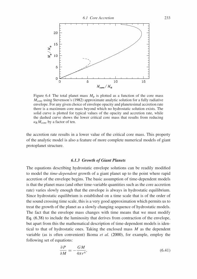
6.1 Core Accretion 233
Figure 6.4 The total planet mass Mp is plotted as a function of the core massMcore using Stevenson’s (1982) approximate analytic solution for a fully radiativeenvelope. For any given choice of envelope opacity and planetesimal accretion ratethere is a maximum core mass beyond which no hydrostatic solution exists. Thesolid curve is plotted for typical values of the opacity and accretion rate, whilethe dashed curve shows the lower critical core mass that results from reducingκRMcore by a factor of ten.
the accretion rate results in a lower value of the critical core mass. This propertyof the analytic model is also a feature of more complete numerical models of giantprotoplanet structure.
6.1.3 Growth of Giant Planets
The equations describing hydrostatic envelope solutions can be readily modifiedto model the time-dependent growth of a giant planet up to the point where rapidaccretion of the envelope begins. The basic assumption of time-dependent modelsis that the planet mass (and other time-variable quantities such as the core accretionrate) varies slowly enough that the envelope is always in hydrostatic equilibrium.Since hydrostatic equilibrium is established on a time scale that is of the order ofthe sound crossing time scale, this is a very good approximation which permits us totreat the growth of the planet as a slowly changing sequence of hydrostatic models.The fact that the envelope mass changes with time means that we must modifyEq. (6.38) to include the luminosity that derives from contraction of the envelope,but apart from this the mathematical description of time-dependent models is iden-tical to that of hydrostatic ones. Taking the enclosed mass M as the dependentvariable (as is often convenient) Ikoma et al. (2000), for example, employ thefollowing set of equations:
∂P
∂M= − GM
4πr4, (6.41)

234 Giant Planet Formation
∂r
∂M= 1
4πr2ρ, (6.42)
∂T
∂M=
{ − 3κR64πσr2T 3
L
4πr2 if radiative,(∂T∂P
)S
(∂P∂M
)if convective,
(6.43)
∂L
∂M= εacc − T
dS
dT, (6.44)
where S is the specific entropy of the gas in the envelope and the energy releasedby infalling planetesimals is assumed to be liberated at the core/envelope interface
εacc = δ(r − Rs)
4πr2ρMcore
∫ rout
Rs
GM
r2dr . (6.45)
As with the hydrostatic solutions, different authors adopt slight variations of theseequations that differ, for example, in the assumed location of the outer boundaryand in where within the envelope the energy of accreted planetesimals is released.These differences are rarely consequential. Of greater importance is the fact thatthe equations for the planetary structure must be supplemented with a model forhow the planetesimal accretion rate Mcore varies with time. The core accretionrate can be calculated using methods similar to those employed in the study ofterrestrial planet growth (Section 5.2) provided that we allow for the fact that theplanet mass must now include both the core and the envelope contributions, andthat the cross-section for accretion may be modified by aerodynamic processeswithin the bound envelope. The mass of heavy elements within the planet will alsoincrease due to pebble accretion. Any uncertainties in the magnitude and evolutionwith time of Mcore (for example due to different assumptions as to the degreeof gravitational focusing) propagate directly into the calculation of giant planetgrowth, and influence both the time scale and feasibility of planet formation at aparticular location within the disk.
The first fully consistent time-dependent models of giant planet growth werepublished by Pollack et al. (1996), and their calculation, reproduced in slightlysimplified form in Fig. 6.5, identified the main phases of the process. For their base-line model Pollack et al. (1996) considered the formation of Jupiter from a core at5.2 AU in a disk with a solid surface density �p = 10 g cm−2 and a gaseous surfacedensity � = 7 × 10² g cm−2. They adopted an opacity in the outer envelope thatwould be appropriate for a solar mixture of small grains that follow an interstellarsize distribution. The model assumed that growth occurs exclusively through plan-etesimal accretion, with no contribution from pebbles. With these assumptions thegrowth of Jupiter proceeds through three well-separated phases:
• Core formation. Initially the core grows very rapidly due to runaway accretionof planetesimals within its feeding zone. The envelope mass remains small, andthe growth of the total mass is dominated by the growth of the core. This phase

6.1 Core Accretion 235
is relatively brief (≈ 0.5 Myr) and comes to an end once the core approaches itsisolation mass.
• Hydrostatic growth. This phase is characterized by the slow accretion of gasfrom the protoplanetary disk. The increasing mass of the planet drives a slowexpansion of the feeding zone which suffices to maintain continued accretion ofplanetesimals, albeit at a lower rate than in the first phase. The hydrostatic phasecontinues for ≈ 7 Myr and ends only when the mass of the envelope starts toapproach the mass of the core.
• Runaway growth. Once Menv>∼ Mcore the rate of accretion accelerates dra-
matically and runaway growth of the envelope sets in. The rate of accretionbecomes limited by the rate at which the disk can supply gas, and is eventuallyshut off either by the onset of local tidal effects (to be discussed in more detail inChapter 7) or by global disk dispersal.
As shown in Fig. 6.5 this model yields a formation time scale for Jupiter of 7–8 Myrand a primordial core mass of Mcore � 20 M⊕.
The Pollack et al. (1996) model is a single member of a broad family of “coreaccretion” models that can form giant planets with a range of properties underdifferent physical conditions. Let us initially retain two of the basic assumptions,
Hydrostatic†growth
Mas
s (
)
( )
C
Figure 6.5 The evolution of the core mass (solid line), envelope mass (dottedline) and total mass (dashed line) from a time-dependent calculation of giantplanet formation via core accretion (Rice & Armitage, 2003). In this illustrativecalculation, which is based on a slightly simplified version of the physics describedin Pollack et al. (1996), a core grows at a fixed radius of 5.2 AU in a diskwith a solid surface density �p = 10 g cm−2 and a gaseous surface density� = 7×10² g cm−2. With this choice of parameters and input physics one obtainsa relatively short-lived phase of core formation that is followed by an extendedperiod of slow coupled growth of the core and envelope. The critical core mass isexceeded and runaway growth starts after about 7–8 Myr, at which time the coremass is approximately 20 M⊕.
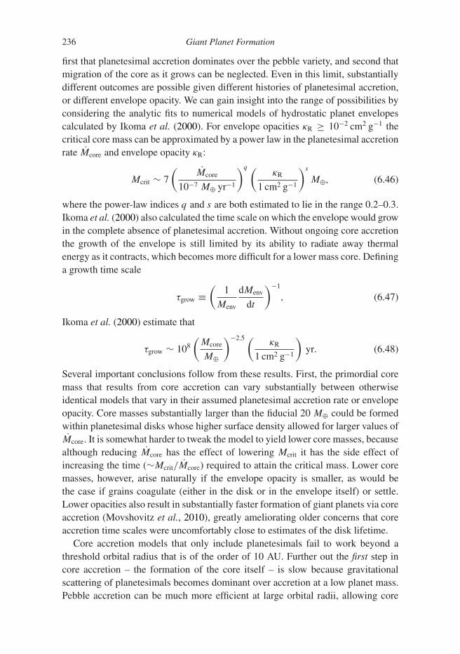
236 Giant Planet Formation
first that planetesimal accretion dominates over the pebble variety, and second thatmigration of the core as it grows can be neglected. Even in this limit, substantiallydifferent outcomes are possible given different histories of planetesimal accretion,or different envelope opacity. We can gain insight into the range of possibilities byconsidering the analytic fits to numerical models of hydrostatic planet envelopescalculated by Ikoma et al. (2000). For envelope opacities κR ≥ 10−2 cm2 g−1 thecritical core mass can be approximated by a power law in the planetesimal accretionrate Mcore and envelope opacity κR:
Mcrit ∼ 7
(Mcore
10−7 M⊕ yr−1
)q (κR
1 cm2 g−1
)s
M⊕, (6.46)
where the power-law indices q and s are both estimated to lie in the range 0.2–0.3.Ikoma et al. (2000) also calculated the time scale on which the envelope would growin the complete absence of planetesimal accretion. Without ongoing core accretionthe growth of the envelope is still limited by its ability to radiate away thermalenergy as it contracts, which becomes more difficult for a lower mass core. Defininga growth time scale
τgrow ≡(
1
Menv
dMenv
dt
)−1
, (6.47)
Ikoma et al. (2000) estimate that
τgrow ∼ 108
(Mcore
M⊕
)−2.5 (κR
1 cm2 g−1
)yr. (6.48)
Several important conclusions follow from these results. First, the primordial coremass that results from core accretion can vary substantially between otherwiseidentical models that vary in their assumed planetesimal accretion rate or envelopeopacity. Core masses substantially larger than the fiducial 20 M⊕ could be formedwithin planetesimal disks whose higher surface density allowed for larger values ofMcore. It is somewhat harder to tweak the model to yield lower core masses, becausealthough reducing Mcore has the effect of lowering Mcrit it has the side effect ofincreasing the time (∼Mcrit/Mcore) required to attain the critical mass. Lower coremasses, however, arise naturally if the envelope opacity is smaller, as would bethe case if grains coagulate (either in the disk or in the envelope itself) or settle.Lower opacities also result in substantially faster formation of giant planets via coreaccretion (Movshovitz et al., 2010), greatly ameliorating older concerns that coreaccretion time scales were uncomfortably close to estimates of the disk lifetime.
Core accretion models that only include planetesimals fail to work beyond athreshold orbital radius that is of the order of 10 AU. Further out the first step incore accretion – the formation of the core itself – is slow because gravitationalscattering of planetesimals becomes dominant over accretion at a low planet mass.Pebble accretion can be much more efficient at large orbital radii, allowing core
6.2 Constraints on the Interior Structure of Giant Planets 237
accretion to form giant planets out to distances of the order of 50 AU (Lambrechts& Johansen, 2012). Indeed, if we allow ourselves the freedom to construct hybridmodels that include both pebble and planetesimal accretion (which can still beimportant as a source of heat to slow down the onset of runaway growth), the rangeof orbital radii and time scales on which giant planets may in principle form is verywide. Theoretically determining what part of that range is actually populated ishard, because pebble variants of core accretion are intrinsically global problems ina way that older planetesimal-based models were not. In particular, core accretionmodels that include pebbles require a quantitative understanding of the abundanceof protoplanetary seeds, the evolution of the radial pebble flux and its accretionon to those seeds, and the dynamical evolution of the cores themselves (Levisonet al., 2015). Improved observational knowledge of the exoplanet population atradii beyond 10 AU will likely be indispensable for an understanding of the physicalprocesses responsible for the formation of wide-separation planetary systems.
The masses that we have been discussing for the pre-runaway phases of coreaccretion correspond closely to those for which orbital migration due to gravita-tional torques exerted by the disk on the planet is particularly rapid (discussed inChapter 7). Migration is expected to alter the predictions of core accretion models inboth their planetesimal and pebble-driven variants. In planetesimal-driven models,the relatively long time between the formation of a few M⊕ core and the onsetof runaway gas accretion means that extensive orbital migration (potentially tovery short-period orbits) is possible within many disk models. The faster growthmade possible by pebbles helps, but the fact that pebble accretion is not a runawayprocess means that migration still cannot be ignored. The main logical possibilitiesare either that radial reshaping of forming giant planet systems due to migration isubiquitous, or that giant planets form preferentially at planet traps where the diskstructure supports convergent radial migration.
6.2 Constraints on the Interior Structure of Giant Planets
The best constraints on core accretion come from the Solar System. Spacecraftmeasurements of the gravitational field, when combined with knowledge of theequation of state and atmospheric composition, can be used to build models of theinterior structure of the Solar System’s giant planets. Individual measurements ofextrasolar planets are much less powerful. The mass–radius relation of giant planetsdepends upon the total mass of heavy elements within the planet, but has littlesensitivity to whether those elements are distributed uniformly within the planetor concentrated within a core. Modeling of the population of extrasolar planets is,in principle, more constraining. The observed correlation between host metallicityand the abundance of giant planets (Section 1.8.4), for example, is qualitativelyconsistent with core accretion expectations and can be investigated quantitativelywithin a full model for giant planet formation and migration.

238 Giant Planet Formation
6.2.1 Interior Structure from Gravity Field Measurements
The interior structures of Jupiter and Saturn can be constrained by comparing theo-retical stucture models to measurements of their gravitational fields. The principleof the method relies upon the fact that rotating giant planets (Jupiter has a rotationperiod of approximately 10 hours) are axially rather than spherically symmetricbodies. The gravitational field outside the planet then depends not just on the planetmass and distance (as is the case for spherical bodies), but also on the distributionof mass within the planet. This connection between the external potential and theinternal structure can be formalized by expanding the potential of a rotating planetin Legendre polynomials (e.g. Guillot et al., 2004):
�(r,θ) = GMp
r
[1 −
∞∑i=1
(Req
r
)2i
J2iP2i(cos θ)
]. (6.49)
Here Req is the planet’s equatorial radius, θ is the angular distance measured fromthe pole, and the P2i are Legendre polynomials. The J2i are called the gravitationalmoments, and these can be measured by modeling the trajectories of spacecraft thatmake flybys or enter orbit about the planet. In practice the series converges rapidlyand only the first few moments are required to yield an accurate description of thegravitational field. For Jupiter, data from the JUNO mission (Iess et al., 2018) havebeen used to measure the even harmonics up to J10. J2 is determined to a precisionof about 1 part in 106, with the precision dropping steadily to about 1% for J8.4
Data from the Cassini mission yield similarly precise measurements of Saturn’sexternal gravity field.
To make use of the measured moments to constrain the internal structure, we notethat they can be written as a volume integral over the planet’s density distribution(e.g. Zharkov & Trubitsyn, 1974):
J2i = − 1
MpR2ieq
∫ρr2iP2i(cos θ)dV . (6.50)
A set of measured moments then yields multiple integral constraints on the densitydistribution that must be satisfied by any physical planet model. The weightingfunction inside the integral means that the higher order moments become increas-ingly sensitive to structure near the surface of the planet rather than to the centralregions.
Even for Jupiter, where the gravitational field data are of exquisite quality, thenumber of observational constraints that bear on the interior structure is quitelimited. We have the total mass, radius, and surface rotation rate, together withfour well-measured even harmonics of the gravity field and knowledge of the
4 JUNO data have also been used to measure the odd harmonics. These measurements do not further constrainthe static interior structure, but instead probe the depth to which dynamic features such as zonal flows extendwithin the planet.
6.2 Constraints on the Interior Structure of Giant Planets 239
atmospheric composition. This reality forces us to exercise careful judgement indetermining what type of theoretical model to compare the data against. There is nohope of measuring the detailed properties of Jupiter’s core in a model-independentway. Rather, the goal is to construct and constrain models that incorporate our bestestimates of the equation of state at the relevant interior pressures, with physicallyreasonable transitions in the structure at different radii.
6.2.2 Internal Structure of Jupiter
Figure 6.6 shows an example interior structure for Jupiter that is consistent withthe available observational constraints (Wahl et al., 2017). The model structure hasfour layers. The envelope has a compositional transition, with a helium-poor upperenvelope, in which hydrogen is molecular, overlying a helium-rich lower envelope,in which hydrogen is metallic. The core also has two layers. A dense inner core,made up of icy and rocky material, blends into a dilute outer core containing amixture of metallic hydrogen and heavy elements.
Compared to earlier generations of models, current determinations of Jupiter’sinternal structure benefit from greatly improved measurements of the gravity fieldand from smaller theoretical uncertainties in the equation of state at high pressure.The mass of heavy elements in the core region is estimated at 7–25 M⊕ (Wahlet al., 2017), with a preference for a dilute core structure of the type previouslysuggested theoretically (Stevenson, 1982; Lissauer & Stevenson, 2007). The large
Molecular hydrogen,helium depleted
Helium rain layer
Metallic hydrogen layer,helium rich
Dense inner core
Dilute outer core
Dissolution and mixing of coreinto surrounding envelope
Figure 6.6 An example of an interior structure model that is compatible withJUNO measurements of Jupiter’s gravitational field (based on Wahl et al, 2017).
240 Giant Planet Formation
error bar reflects degeneracies in the predictions of different theoretical models, andthe fundamental difficulty of determining the deep interior structure of a planet fromonly exterior data, without benefit of the powerful seismic data that are available forthe Earth and the Sun. The estimated core mass is consistent with the expectationsof core accretion theory, but spans too wide a range to discriminate between differ-ent physically reasonable variants.
6.3 Disk Instability
Gaseous protoplanetary disks may undergo a phase in which they are massiveenough to be unstable to instabilities arising from their own self-gravity. If theoutcome of these instabilities is fragmentation, disk instability could be a channelfor the formation of massive planets, brown dwarfs, or binary stellar systems. Thereis a long history of suggestions that disk instability could form planets, datingback to models by Kuiper (1951) and Cameron (1978) that predate any seriouswork on core accretion. More recent work by Boss (1997) was the foundationfor renewed interest in disk instability models. As a possible planet formationprocess, the fundamental difference between the disk instability model and thecore accretion model arises from the fact that in the disk instability model thesolid component of the disk is a bystander that plays only an indirect role (viaits contribution to the opacity) in the process of planet formation.
We have already derived the conditions needed for a protoplanetary gas disk tobecome unstable to its own self-gravity in Sections 3.4 and 4.6.1. Globally the diskmass must roughly satisfy
Mdisk
M∗>∼
h
r, (6.51)
while the well-defined local condition is
Q ≡ cs�
πG�< Qcrit, (6.52)
where Qcrit is a dimensionless measure of the threshold below which instabilitysets in. It lies in the range 1 < Qcrit < 2. If we compare these requirements toobservational determinations of protoplanetary disk properties the global conditionsuggests that widespread gravitational instability (i.e. instability that extends acrossa large range of disk radii) must be limited to disks at the upper end of the observedrange, with masses of around a tenth of the stellar mass. Such massive disks maybe commonly present early in the evolution of pre-main-sequence stars (e.g. Eisneret al., 2005). For a disk around a solar mass star the local condition can be writtenin the form
� >∼ 3.8 × 10³
(Qcrit
1.5
)−1 (h/r
0.05
)( r
5 AU
)−2g cm−2. (6.53)
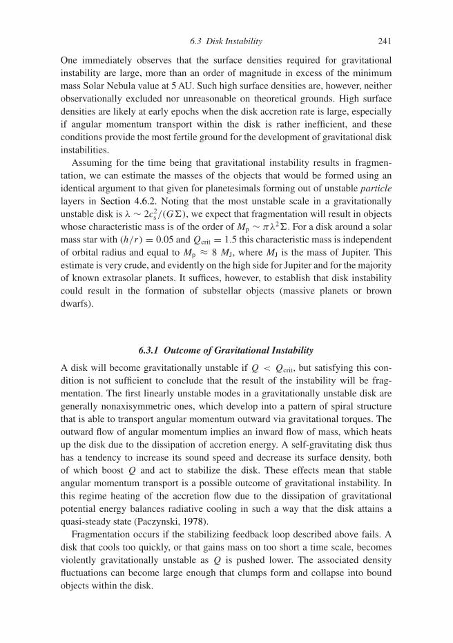
6.3 Disk Instability 241
One immediately observes that the surface densities required for gravitationalinstability are large, more than an order of magnitude in excess of the minimummass Solar Nebula value at 5 AU. Such high surface densities are, however, neitherobservationally excluded nor unreasonable on theoretical grounds. High surfacedensities are likely at early epochs when the disk accretion rate is large, especiallyif angular momentum transport within the disk is rather inefficient, and theseconditions provide the most fertile ground for the development of gravitational diskinstabilities.
Assuming for the time being that gravitational instability results in fragmen-tation, we can estimate the masses of the objects that would be formed using anidentical argument to that given for planetesimals forming out of unstable particlelayers in Section 4.6.2. Noting that the most unstable scale in a gravitationallyunstable disk is λ ∼ 2c2
s /(G�), we expect that fragmentation will result in objectswhose characteristic mass is of the order of Mp ∼ πλ2�. For a disk around a solarmass star with (h/r) = 0.05 and Qcrit = 1.5 this characteristic mass is independentof orbital radius and equal to Mp ≈ 8 MJ, where MJ is the mass of Jupiter. Thisestimate is very crude, and evidently on the high side for Jupiter and for the majorityof known extrasolar planets. It suffices, however, to establish that disk instabilitycould result in the formation of substellar objects (massive planets or browndwarfs).
6.3.1 Outcome of Gravitational Instability
A disk will become gravitationally unstable if Q < Qcrit, but satisfying this con-dition is not sufficient to conclude that the result of the instability will be frag-mentation. The first linearly unstable modes in a gravitationally unstable disk aregenerally nonaxisymmetric ones, which develop into a pattern of spiral structurethat is able to transport angular momentum outward via gravitational torques. Theoutward flow of angular momentum implies an inward flow of mass, which heatsup the disk due to the dissipation of accretion energy. A self-gravitating disk thushas a tendency to increase its sound speed and decrease its surface density, bothof which boost Q and act to stabilize the disk. These effects mean that stableangular momentum transport is a possible outcome of gravitational instability. Inthis regime heating of the accretion flow due to the dissipation of gravitationalpotential energy balances radiative cooling in such a way that the disk attains aquasi-steady state (Paczynski, 1978).
Fragmentation occurs if the stabilizing feedback loop described above fails. Adisk that cools too quickly, or that gains mass on too short a time scale, becomesviolently gravitationally unstable as Q is pushed lower. The associated densityfluctuations can become large enough that clumps form and collapse into boundobjects within the disk.

242 Giant Planet Formation
6.3.2 Cooling-Driven Fragmentation
We can express the cooling criterion for fragmentation in two equivalent ways,which, taken together, expose the important physics. The essential argument isbased upon the fact that, if cooling is very rapid, gravitational instabilities must berather violent to generate heating that is sufficient to mitigate these losses. Quanti-tatively we can define a local cooling time scale via
tcool ≡ U
|dU/dt |, (6.54)
where U is the thermal energy content of the disk per unit area, and ask what is theequivalent value of α that would be required to generate enough offsetting heating.As we showed in Section 3.4.2 the answer is
α = 4
9γ (γ − 1)�tcool, (6.55)
where γ is the two-dimensional adiabatic index (Gammie, 2001). The equivalentα (a measure of the strength of the “self-gravitating turbulence” within the disk) isthus inversely proportional to the cooling time. We should caution that this simpleresult relies on the assumption that turbulence and transport within the disk is local.Since gravitational torques can act over long ranges one should worry about this, butin practice subsequent work shows that the formally local result is approximatelyvalid for many conditions of interest for protoplanetary disks.
Noting that when α ∼ 1 the velocity perturbations within the disk becomesupersonic, we might guess that this would be when transient clumps would becomedense enough to collapse and trigger fragmentation. This intuition is roughly cor-rect. Early numerical simulations by Gammie (2001) showed that for a particularequation of state there is a critical cooling time scale below which fragmentationoccurs. For γ = 2,
tcool, crit � 3�−1. (6.56)
Subsequent work identified subtleties in obtaining a numerical converged estimateof tcool, crit, but later determinations are broadly in agreement with the original valueof tcool, crit � 3�−1 (Deng et al., 2017; Baehr et al., 2017). The critical cooling timecorresponds to a critical value of the equivalent α that divides the regimes of stableangular momentum transport from fragmentation:
αcrit � 0.1. (6.57)
A locally self-gravitating disk cannot sustain a larger α without fragmenting (Riceet al., 2005).
The disk mass above which a disk becomes gravitationally unstable is equal (upto numerical factors) to the mass above which self-gravity provides the dominant
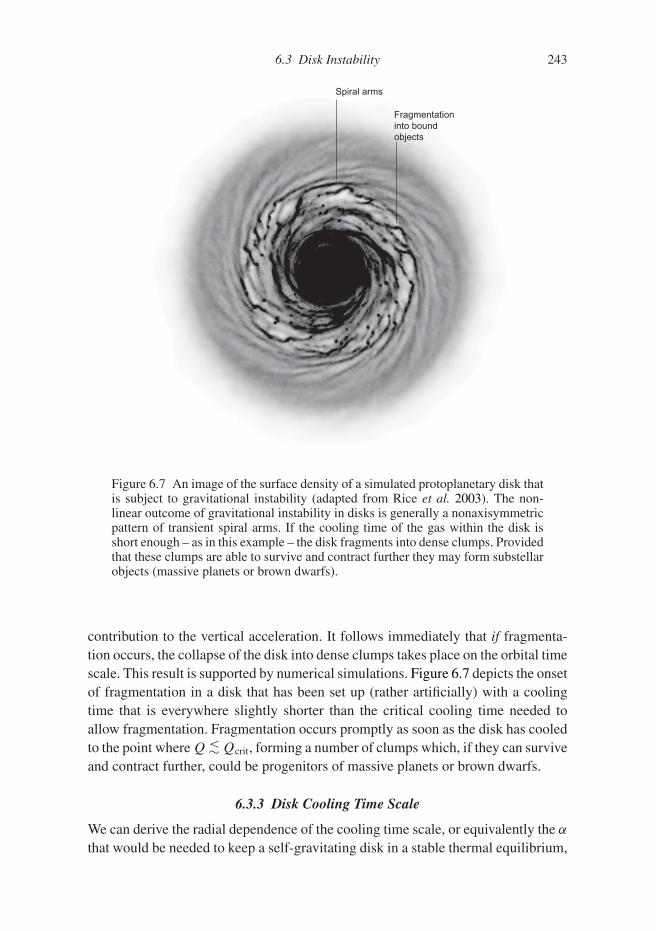
6.3 Disk Instability 243
Spiral arms
Fragmentation into boundobjects
Figure 6.7 An image of the surface density of a simulated protoplanetary disk thatis subject to gravitational instability (adapted from Rice et al. 2003). The non-linear outcome of gravitational instability in disks is generally a nonaxisymmetricpattern of transient spiral arms. If the cooling time of the gas within the disk isshort enough – as in this example – the disk fragments into dense clumps. Providedthat these clumps are able to survive and contract further they may form substellarobjects (massive planets or brown dwarfs).
contribution to the vertical acceleration. It follows immediately that if fragmenta-tion occurs, the collapse of the disk into dense clumps takes place on the orbital timescale. This result is supported by numerical simulations. Figure 6.7 depicts the onsetof fragmentation in a disk that has been set up (rather artificially) with a coolingtime that is everywhere slightly shorter than the critical cooling time needed toallow fragmentation. Fragmentation occurs promptly as soon as the disk has cooledto the point where Q <∼ Qcrit, forming a number of clumps which, if they can surviveand contract further, could be progenitors of massive planets or brown dwarfs.
6.3.3 Disk Cooling Time Scale
We can derive the radial dependence of the cooling time scale, or equivalently the α
that would be needed to keep a self-gravitating disk in a stable thermal equilibrium,

244 Giant Planet Formation
by combining a model for the disk structure with the requirement that Q ∼ 1(Levin, 2007). We assume that a self-gravitating disk maintains
Q = cs�
πG�= Q0, (6.58)
and combine that with the equation for the sound speed c2s = kBTc/μmp to get an
expression for the central disk temperature:
Tc = π2Q20G
2
(μmp
kB
)�2
�2. (6.59)
To assess the stability of the disk we need to determine how quickly a disk with agiven central temperature and surface density would cool. For a simple example, weassume that the disk is at least moderately optically thick, and that the form of theopacity law has the T 2
c dependence expected for ice grains. The relation betweenthe central temperature Tc and the effective temperature Tdisk then follows from theequations (Section 3.3.3)
T 4c
T 4disk
= 3
4τ, (6.60)
τ = 1
2κR�, (6.61)
κR = κ0T2
c . (6.62)
The cooling rate is then
dU
dt= 2σT 4
disk = 16σ
3κ0�T 2
c . (6.63)
Noting that the thermal energy content of the disk per unit area is
U = c2s �
γ (γ − 1), (6.64)
Eqs. (6.54) and (6.55) allow us to find how α scales with the disk parameters:
α = 64
27
(μmp
kB
)2π2Q2
0σG2
κ0�−3. (6.65)
For this opacity law the only parameter that matters for the stress is the angularvelocity �.
Substituting some reasonable numbers, κ0 = 2×10⁻⁴ cm2 g−1 K−2 and Q0 = 1.5,the result for a solar mass star is
α ∼ 0.1( r
40 AU
)9/2. (6.66)

6.3 Disk Instability 245
Comparing this result to the estimate of the maximum stress that a self-gravitatingdisk can stably support (Eq. 6.57) the conclusion is that fragmentation is not pos-sible in the inner disk, but may occur at radii between about 40 AU and 100 AU(Clarke, 2009; Rafikov, 2009).
The radii where fragmentation may be possible coincide with those where stellarirradiation, rather than heating due to accretion, normally controls the thermal stateof the disk gas. This requires a revision to the argument given above, most obviouslybecause if � is too small stellar irradiation may be able to keep Q � 1 and preventthe disk becoming self-gravitating in the first place. More generally, the possibil-ity of significant stellar irradiation needs to be considered in most circumstanceswhere protoplanetary disks are gravitationally unstable (Rice et al., 2011; Hirose &Shi, 2019).
6.3.4 Infall-Driven Fragmentation
Our analysis of thermally driven fragmentation implicitly assumed the type ofrelatively isolated disk that is found in Class 2 YSOs. Common sense, however,suggests that the massive disks that might be gravitationally unstable are morelikely to be present in the youngest Class 0 or Class 1 YSOs. In these systemsthe disks are not isolated, but instead are being actively fed with mass that is fallingin from an envelope. This feeding, if it is too rapid, provides an alternative way toforce a gravitationally unstable disk to fragment. Mass addition to the disk on a fasttime scale can exceed the ability of self-gravity to transport mass inward, leavingfragmentation as the only other possibility.
Numerical results on the conditions for infall-driven fragmentation can be moti-vated by thinking about two distinct senses in which infall might be “too rapid.”For a system with a total mass Mtotal = M∗ + Mdisk, a characteristic global timescale for the infalling gas is �−1, where the angular frequency is measured at thecircularization radius given the mean specific angular momentum of the envelope.A dimensionless parameter expressing the strength of infall is therefore
� ≡ Minfall
Mtotal�−1. (6.67)
A second relevant parameter can be defined by thinking about the ability of aself-gravitating disk to attain a steady-state by transporting the infalling gas awayquickly enough. Setting Q = Q0 as before, making use of the α prescription(ν = αc2
s /�), and noting that in a steady-state disk ν� = M/(3π), the transportrate through a self-gravitating disk is
M = 3πα
Q0
c3s
G. (6.68)
Based on this, we can can express the “strength” of the self-gravitating transportthat is needed to stably remove mass being added at a rate Minfall via a parameter
246 Giant Planet Formation
ξ ≡ GMinfall
c3s
. (6.69)
For a thin disk ξ ∝ α, and we could use the same line of reasoning as for thermallyunstable disks to argue that fragmentation ought to occur when α exceeds somethreshold value. We can still define ξ , however, in more general situations (forexample when the disk mass exceeds the stellar mass) where the approximationsinvolved in treating self-gravitating disks as pseudo-viscous structures break down.
Numerical simulations of isothermal disks undergoing infall show that the frag-mentation condition can be expressed in terms of � and ξ . Kratter et al. (2010) findthat fragmentation occurs when
� <∼ 1.2 × 10⁻³ξ 2.5. (6.70)
Kratter and Lodato (2016), and references therein, provide additional details on thisregime of fragmentation.
6.3.5 Outcome of Disk Fragmentation
The range of outcomes that result from the fragmentation of gravitationally unsta-ble disks is not well known. Observations of L1448 IRS3B show that the threeprotostars in the system co-exist with a disk showing spiral structure indicative ofgravitational instability (Tobin et al., 2016). This observation, together with lessdirect arguments based on larger samples of stars, suggests that disk fragmentationis a mechanism for forming binaries and other multiple stellar systems. It is consis-tent with the basic theoretical expectation that fragments, forming in a massive andhighly turbulent disk, would often accrete rapidly from the remaining disk material.
Substellar companions (brown dwarfs or massive planets) may also be outcomesof disk fragmentation, especially if it takes place at a somewhat later epoch whenthe disk is less massive. Accretion on to clumps formed from fragmentation willbe suppressed if the time scale for them to cool and contract is long, and may befurther reduced (or even reversed) if the clumps migrate inward and lose their outerenvelopes to tidal shear (Nayakshin, 2010). From an observational perspective, noextrasolar planetary systems are known whose properties unambiguously point toan origin from disk instability. Systems of one or more very massive planets, orbit-ing at the radii between about 50 AU and 200 AU characteristic of fragmentation,are the most obvious candidates, and a number of examples of these have beendiscovered.
6.4 Further Reading
“Formation of Giant Planets,” G. D’Angelo & J. J. Lissauer (2018), in Handbook of Exo-planets. Cham: Springer, id. 140.
“Gravitational Instabilities in Circumstellar Disks,” K. Kratter & G. Lodato (2016), AnnualReview of Astronomy and Astrophysics, 54, 271.

7
Early Evolution of Planetary Systems
The classical theory of giant planet formation described in the preceding chapterpredicts that massive planets ought to form on approximately circular orbits, witha strong preference for formation in the outer disk at a few AU or beyond. Mostcurrently known extrasolar planets have orbits that are grossly inconsistent withone or the other of these predictions. Even within the Solar System the existence ofa large resonant population of Kuiper Belt Objects, including Pluto, is inconsistentwith a model in which the giant planets formed in the same orbits that they currentlyinhabit.
In this chapter we describe a set of physical mechanisms – often genericallydescribed as migration processes – that can lead to the modification of plane-tary orbits. Any process that allows a planet to exchange energy and/or angularmomentum with another component of the system will lead to migration, and thereare several contenders. The other party can be the gas, planetesimal, or particledisk, another planet, the host star, or a binary companion. If substantial enough,migration can make the final architecture of the system unrecognizable from itsstate immediately after planet formation.
The study of planetary migration involves two sets of challenges. The first is tounderstand the physics of individual processes well enough that theoretical uncer-tainties are not the dominant limitation when building models of observed systems.To take an example, determining the rate of change of the semi-major axis of a3 M⊕ planet embedded in a protoplanetary gas disk of given properties (and withspecified physics) is a well-posed problem. Recent years have seen substantialprogress in solving these types of problems. The second challenge is harder. Whichprocesses dominated or contributed substantially to the observed architecture oftypical planetary systems, or to specific examples such as the Solar System? This isharder because a model that includes several physical processes is only as reliableas its weakest link, and because, with imperfect knowledge of the initial condi-tions, we are forced to rely on late-time observations that may not contain enoughinformation to uniquely reconstruct the earlier history. Many of the observationsthat motivate study of migration can, as a result, be fit with more than one model.
247
248 Early Evolution of Planetary Systems
7.1 Migration in Gaseous Disks
Gas disk migration refers to a change in the semi-major axis of a planet that iscaused by exchange of angular momentum between the planet and the surroundinggaseous protoplanetary disk. The exchange of angular momentum is mediated bygravitational torques between the planet and the disk. No torque is exerted on aplanet by an axisymmetric disk, so gas disk migration can only take place if theplanet excites nonaxisymmetric structure. In addition to angular momentum, energyis also exchanged between the planet and the disk, and depending upon the detailsof these exchanges the net result may be changes not just in a but also in e and i.
Migration is potentially important whenever a fully formed planet (very roughlyof the mass of Mars or above – smaller bodies do not interact strongly with thedisk) co-exists with a gaseous disk. Such co-existence is inevitable for the coresof giant planets forming via core accretion, and for gas giants themselves, and thepossibility of large-scale gas disk migration can never be ignored when consideringthe formation of these objects. For terrestrial planets (including super-Earths inextrasolar planetary systems) the likely importance of gas disk migration is modeldependent. In the classical scenario for terrestrial planet formation in the SolarSystem, the time scale for the final assembly of the terrestrial planets substantiallyexceeds the typical gas disk lifetime. It is then possible that the progenitors of ourterrestrial planets remained of sufficiently low mass prior to disk dispersal thatmigration can be consistently ignored. Similar or more massive planets formingat smaller orbital radii, where the growth time scale is shorter, would instead fallinto the regime where planet–disk interactions need to be considered.
7.1.1 Planet–Disk Torque in the Impulse Approximation
The detailed physics of the gravitational interaction between a planet and a sur-rounding gas disk is subtle, and several important aspects remain poorly under-stood. To gain some insight into the interaction it is useful to begin by consideringa gaseous analog of the two-body dynamics discussed in the context of terrestrialplanet formation in Section 5.3.1. We assume that a particle in the gas disk isinitially on an unperturbed circular orbit, and calculate the angular momentumchange that occurs as the particle is impulsively deflected during a close approachto the planet. The deflection is calculated as if the particle in the gas disk were afreely moving test particle, and hydrodynamics is ignored entirely except for theimplicit assumption that the disk is able to “smooth out” the trajectories so thatparticles resume unperturbed orbits prior to making their next encounter with theplanet. Despite these simplifications, calculation of the planet–disk interaction viathe so-called impulse approximation (Lin & Papaloizou, 1979) yields correct scal-ings and better than order of magnitude estimates of the rate of angular momentumtransport.

7.1 Migration in Gaseous Disks 249
Working in a frame of reference moving with the planet, we consider the grav-itational interaction between the planet and gas flowing past with relative velocity�v and impact parameter b. We have already derived (in the two-body, free particlelimit) the change to the perpendicular velocity that occurs during the encounter. It is(Eq. 5.58)
|δv⊥| = 2GMp
b�v, (7.1)
where Mp is the planet mass. This velocity is directed radially, and hence doesnot correspond to any angular momentum change. The interaction in the two-bodyproblem is however conservative, so the increase in the perpendicular velocityimplies a reduction (in this frame) of the parallel component. Equating the kineticenergy of the gas particle well before and well after the interaction has taken placewe have that
�v2 = |δv⊥|2 + (�v − δv‖)2, (7.2)
which implies (for small deflection angles)
δv‖ � 1
2�v
(2GMp
b�v
)2
. (7.3)
If the planet has a semi-major axis a the implied angular momentum change perunit mass of the gas is
�j = 2G2M2pa
b2�v3. (7.4)
It is worth pausing at this juncture to fix the sign of the angular momentum changeexperienced by the gas and by the planet firmly in our minds. Gas exterior tothe planet’s orbit orbits the star more slowly than the planet, and is therefore“overtaken” by the planet. The decrease in the parallel component of the relativevelocity of the gas therefore corresponds to an increase in the angular momentumof the gas exterior to the planet. Since the gravitational torque must be equal andopposite for the planet the sign is such that:
• Interaction between the planet and gas exterior to the orbit increases the angularmomentum of the gas, and decreases the angular momentum of the planet. Theplanet will tend to migrate inward, and the gas will be repelled from the planet.
• Interaction with gas interior to the orbit decreases the angular momentum of thegas and increases that of the planet. The interior gas is also repelled, but the planettends to migrate outward.
In the common circumstance where there is gas both interior and exterior to theorbit of the planet, the net torque (and sense of migration) will evidently dependupon which of the above effects dominates.
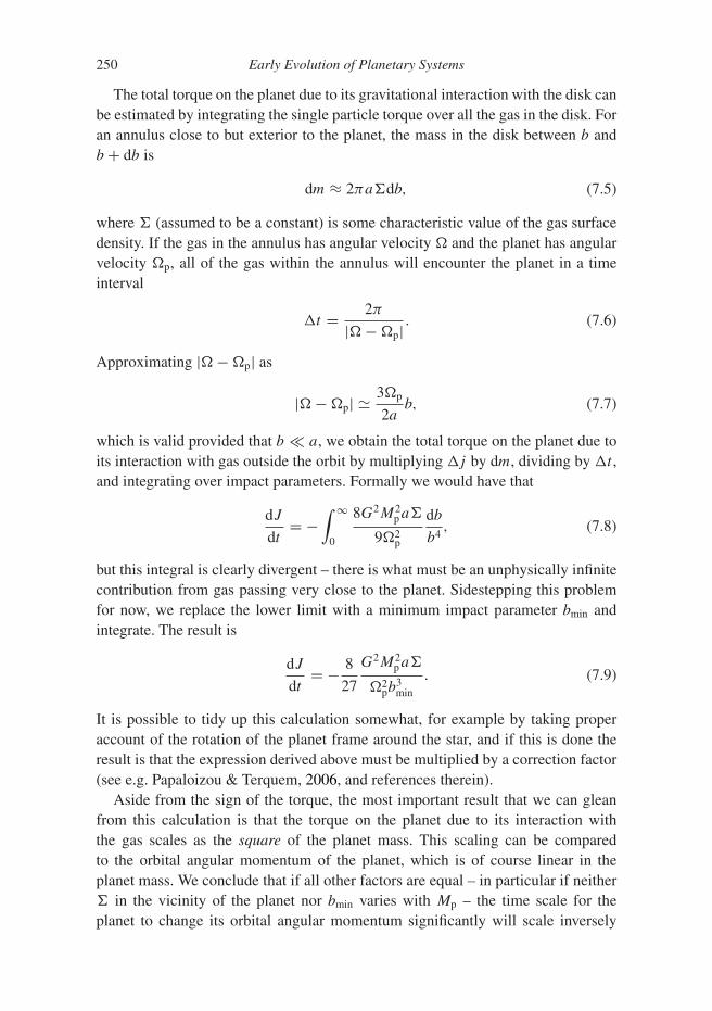
250 Early Evolution of Planetary Systems
The total torque on the planet due to its gravitational interaction with the disk canbe estimated by integrating the single particle torque over all the gas in the disk. Foran annulus close to but exterior to the planet, the mass in the disk between b andb + db is
dm ≈ 2πa�db, (7.5)
where � (assumed to be a constant) is some characteristic value of the gas surfacedensity. If the gas in the annulus has angular velocity � and the planet has angularvelocity �p, all of the gas within the annulus will encounter the planet in a timeinterval
�t = 2π
|� − �p| . (7.6)
Approximating |� − �p| as
|� − �p| � 3�p
2ab, (7.7)
which is valid provided that b a, we obtain the total torque on the planet due toits interaction with gas outside the orbit by multiplying �j by dm, dividing by �t ,and integrating over impact parameters. Formally we would have that
dJ
dt= −
∫ ∞
0
8G2M2pa�
9�2p
db
b4, (7.8)
but this integral is clearly divergent – there is what must be an unphysically infinitecontribution from gas passing very close to the planet. Sidestepping this problemfor now, we replace the lower limit with a minimum impact parameter bmin andintegrate. The result is
dJ
dt= − 8
27
G2M2pa�
�2pb
3min
. (7.9)
It is possible to tidy up this calculation somewhat, for example by taking properaccount of the rotation of the planet frame around the star, and if this is done theresult is that the expression derived above must be multiplied by a correction factor(see e.g. Papaloizou & Terquem, 2006, and references therein).
Aside from the sign of the torque, the most important result that we can gleanfrom this calculation is that the torque on the planet due to its interaction withthe gas scales as the square of the planet mass. This scaling can be comparedto the orbital angular momentum of the planet, which is of course linear in theplanet mass. We conclude that if all other factors are equal – in particular if neither� in the vicinity of the planet nor bmin varies with Mp – the time scale for theplanet to change its orbital angular momentum significantly will scale inversely

7.1 Migration in Gaseous Disks 251
with the planet mass. The migration velocity in this limit will then be proportional toMp – more massive planets will migrate faster.
Finally, we can estimate the magnitude of the torque for parameters appropriateto different stages of giant planet formation. First, let us consider a rather low masscore (Mp = M⊕) growing at 5 AU in a gas disk of surface density � = 102 g cm−2
around a solar mass star. Our treatment of the interaction has assumed that the diskcan be treated as a two-dimensional sheet, so it is arguably natural to take as aminimum impact parameter bmin = h ≈ 0.05a. Using these numbers we find thatthe exterior torque would drive inward migration on a time scale
τ = J
|dJ/dt | ∼ 1 Myr. (7.10)
Of course this will be partly offset by the interior torque – which has the oppositesign – but unless there is some physical reason why these two torques should cancelto high precision, we would predict changes to the semi-major axis on a time scaleof the order of a Myr. This is already rapid enough to be a potentially importanteffect during giant planet formation via core accretion. Second, we can evaluate thetorque for a fully formed gas giant. A Jupiter mass planet has a Hill sphere rH > h,so it seems reasonable to argue that the value of bmin that we adopted for an Earthmass core is too small in this case. Picking a modestly larger value bmin = 0.2a
results in a time scale,1
τ ∼ 2 × 10⁵ yr, (7.11)
that is an order of magnitude shorter than typical protoplanetary disk lifetimes.If these estimates can be trusted to even an order of magnitude the inescapableconclusion is that gas disk migration ought to be an important process for the earlyevolution of the orbits of giant planets.
7.1.2 Physics of Gas Disk Torques
The impulse approximation provides valuable intuition about planet–disk interac-tions, but does not capture all of the physical effects that can lead to migrationtorques. The total torque is the sum of at least three distinct processes, depicted inFigs. 7.1 and 7.2, torques exerted at Lindblad resonances, co-orbital torques, andadditional torques from the vicinity of the planet due to thermal effects.
The torque component that is easiest to compute accurately arises from wavesthat are excited by the planet’s gravitational perturbation at the location of Lindblad
1 Physically the need to pick a larger value of bmin for a massive planet comes about precisely because theinteraction close to the planet is strong – strong enough in fact to repel all the nearby gas so that there isnothing left for the planet to interact with. We will quantify this effect later, but for now the precise valueof bmin can be considered either as an arbitrary but plausible guess, or as having been chosen with the boguswisdom that comes from knowing the “right” answer so as to yield sensible estimates.
252 Early Evolution of Planetary Systems
Closed streamlinesin horseshoeregion
Co-orbitalregion
Lindbladresonances
Lindbladresonances
Waveexcitation
Figure 7.1 Illustration (not to scale) of disk locations where the purely gravita-tional perturbation of a planet leads to gas disk migration torques. The excitationof waves at exterior Lindblad resonances removes angular momentum from theplanet, while waves launched at interior Lindblad resonances add angular momen-tum. In the co-rotating frame gas close to the planet follows closed horseshoestreamlines. Asymmetries in this region contribute additional co-rotation torques.
resonances. A Lindblad resonance occurs at a radius where gas in the disk is excitedat a frequency that matches that of radial (or epicyclic) oscillations. If the planet hasa circular orbit with angular frequency �p, and the gas disk has orbital frequency�(r) and epicyclic frequency κ(r), the resonant condition is
m[�(r) − �p] = ±κ(r), (7.12)
where m is an integer. For a Keplerian disk the epicyclic and orbital frequencies areidentical and the nominal locations of Lindblad resonances are given by
rL =(
1 ± 1
m
)2/3
a, (7.13)
where a is the semi-major axis of the planetary orbit. This simple expression isvalid if the effects of pressure and self-gravity in the gas disk are negligible. TheLindblad resonances resemble a “comb” and become closely spaced (both to theinside and to the outside) near to the location of the planet.

7.1 Migration in Gaseous Disks 253
Hor
sesh
oe re
gion
Highentropy
Lowentropy
r
f
r > r(r) r < r(r)
Circulating orbit
Librating orbit
Heat flow from luminous planet
Planet
Figure 7.2 Illustration of two of the processes that can lead to torque from thevicinity of the co-orbital region. Gas librating on horseshoe orbits may executehorseshoe turns on a time scale that is faster than the thermal equilibration timewith the background disk. This can result in an azimuthal density asymmetryclose to the planet, and a net torque. Heat from a luminous planet will diffusenonspherically due to shear in the disk. The resulting density perturbation canalso be asymmetric, resulting in a thermal torque.
The Lindblad torque was computed in the context of interactions between satel-lites and planetary rings by Goldreich and Tremaine (1979, 1980), and the calcu-lation has been revisited and refined many times since. In outline, the calculationhas two steps. First, the perturbation to the gravitational potential caused by theplanet is decomposed into Fourier modes that vary azimuthally as exp[im(φ−�pt)],where m is an azimuthal wavenumber. Second, the response of the gas disk to theperturbations is calculated from the linearized hydrodynamic equations, from whichcan be derived the torque.2 The key characteristics of the Lindblad torque are:
• The total torque on the planet is the signed sum of the torque exerted at eachresonant location. The planet gains angular momentum from the interaction withthe inner Lindblad resonances, and loses angular momentum to the outer ones,so there is a partial cancellation. When the effects of pressure in the gas disk areincluded the torque is cut off within a distance �r ≈ 2h/3 of the planet, removingthe apparent divergence that was present in the impulse approximation.
• The planetary perturbation excites waves at the resonant locations, which prop-agate radially and deposit their angular momentum elsewhere in the disk. Thepropagating waves generate the spiral pattern that is seen in numerical simulationsof planet–disk interactions. How the waves propagate and dissipate depends upondetails of the disk structure, but the torque itself is not sensitive to these details.
• The torque does depend upon how far the inner and outer Lindblad resonancesare from the planet, and on the surface density at each resonant location. As a
2 Although the principles are easy to state, the actual calculation is quite intricate. For the reader interested in thedetails the derivation in Meyer-Vernet and Sicardy (1987) is reasonably compact and self-contained.
254 Early Evolution of Planetary Systems
consequence the net torque has a dependence on the gradients (or more generally,the profiles) of surface density and temperature. However, for almost all physicaldisk models the outer resonances exert a greater torque on the planet than theinner ones.
Numerical simulations confirm that linear theory yields a good estimate of the nettorque resulting from planet–disk interactions at Lindblad resonances. The strengthof the torque depends upon how the disk responds to the exchange of angularmomentum with the planet, which in turn depends upon the angular momentumtransport and loss processes acting within the disk. We have noted previously thatthese aspects of disk physics are hard to calculate or measure observationally.However, for planets whose mass is low enough that the disk remains almost unper-turbed, the robust expectation is that the Lindblad torque component results ininward migration (Ward, 1997).
A second component of the torque arises from gravitational perturbations to thegas disk in the co-orbital (or co-rotation) region. A part of the co-rotation torquecan be calculated in an analogous manner to the Lindblad torque, by consideringthe linear response of the gas disk at the location of the co-rotation resonance where�(r) = �p. The linear co-rotation torque depends upon the gradient of vortensity(∇ × v)/� in the disk, and happens to vanish for the minimum-mass Solar Nebulacase where �(r) ∝ r−3/2.
The linear co-rotation torque is not the entirety of the torque exerted in theco-orbital region, even for planet masses low enough to leave the disk surface den-sity unaffected. A second part arises from the interaction of gas on closed horseshoeorbits with the planet (Ward, 1991). Horseshoe orbits, illustrated in Fig. 7.1, arisein the restricted three-body problem but can also be present in fluid disks. It is clearthat fluid elements executing horseshoe orbits must continually exchange angularmomentum with the planet. A parcel of gas that catches up with the planet on aslightly interior orbit must gain angular momentum to move to the exterior orbit,and the reverse process occurs in the switch from the exterior to interior part of thehorseshoe trajectory. In the purely gravitational case of a near-co-orbital particlethe gains and losses sum to zero, and there is no overall torque on the planet. Inthe case of a fluid disk, however, it is possible to generate a persistent asymmetrysuch that the gain in angular momentum during one of the horseshoe turns differsin magnitude from the loss during the other. Any such asymmetry leads to a nettorque on the planet.
A specific example of physics that can generate a horseshoe asymmetry is shownin Fig. 7.2. Suppose that the disk in the vicinity of the planet has a radial gradientof entropy that differs from the adiabatic gradient, and that the time scale for a fluidelement to come into thermal equilibrium is similar to or longer than the time ittakes to complete a horseshoe turn. Under these conditions, the expansion of fluidmoving from the inner portion of the horseshoe outward is not symmetric with

7.1 Migration in Gaseous Disks 255
the compression that occurs moving in the other direction. An azimuthal densityperturbation is set up near the planet, which leads to a torque.
Entropy gradients are not the only cause of a nonzero horseshoe drag. Vortensitygradients are also important, so the total torque depends upon the surface den-sity gradient, the temperature gradient, and thermodynamic properties of the fluid(including its adiabatic index and ability to equilibrate via radiative or diffusiveprocesses).
Evaluating the co-orbital torques using the unperturbed disk structure and ther-modynamic properties as a background yields what is described as the unsaturatedtorque. This is the instantaneous torque that would be experienced by a planetlaid down within a specified disk model. Over time, however, the torque wouldsignificantly modify the angular momentum of fluid on the horseshoe orbits, whichare closed and do not connect to other orbits within the disk. Numerical simula-tions show that in the absence of diffusion and viscosity, the back-reaction on theco-orbital region leads to the torque saturating, and eventually being driven to zero.This phenomenon introduces an implicit dependence of the corotation torque on thestrength of angular momentum transport and loss processes within the disk.
To summarize, a planet experiences torque due to the gravitational perturbationit exerts on near-co-orbital gas as a consequence of several effects. There is alinear co-rotation torque, which depends upon the radial gradient of vortensity, andnonlinear horseshoe drag torques, which vary according to the gradients of surfacedensity and temperature. These torques can only be persistent if there is sufficientdiffusion (or loss) of heat and angular momentum to keep the co-orbital regionunsaturated.
A minimal accounting of planetary migration requires consideration of the signand magnitude of the combined Lindblad and co-rotation torques. There can alsobe other contributions. A luminous planet generates a thermal perturbation in thesurrounding disk, which sources a corresponding density perturbation. If the densityperturbation is asymmetric, the result is a thermal torque. For a planet that is alreadymigrating, the flow of gas through the co-orbital region generates a dynamicaltorque that differs from that experienced by a stationary planet.
7.1.3 Torque Formulae
The results of analytic calculations and simulations of planet–disk interactions canbe represented via formulae that give the magnitude and dependence of the migra-tion torque on the planet. For a disk with a power-law scaling of surface densitywith radius,
�(r) ∝ r−α, (7.14)
the net Lindblad torque on a planet of mass Mp in a circular orbit at distance a fromthe star is given in linear theory as (Tanaka et al., 2002)

256 Early Evolution of Planetary Systems
�LR = −(2.34 − 0.1α)�0, (7.15)
where �0, the reference torque, is,
�0 =(
Mp
M∗
)2 (h
r
)−2
�a4�2K. (7.16)
Comparing the scalings here to those derived via the impulse approximation, wefind that the more sophisticated calculation of the linear theory torque yields adependence on the disk thickness that scales as (h/r)−2 rather than (h/r)−3. Thereason for this difference is that the intrinsic asymmetry between the inner andouter Lindblad torques is itself an increasing function of the disk thickness. Theremaining scalings with planet mass, disk surface density, and orbital radius, areidentical to those deduced from elementary arguments.
The linear part of the co-rotation torque also scales with the disk and planetproperties as a numerical multiple of the reference torque �0. We do not quotethe corresponding formulae, because it is rarely appropriate to consider the linearco-rotation torque without simultaneously accounting for the multiple componentsof the horseshoe drag. Fitting formulae for the latter, and for functions that repre-sent the transition between unsaturated and saturated co-orbital torques, have beenderived numerically, but they are more complex and remain subject to possible revi-sion as simulations improve. The reader who needs accurate estimates of planetarymigration torques is advised to start with current (at the time of writing) papers andreviews by Paardekooper et al. (2011), Kley and Nelson (2012), and Jimenez andMasset (2017), and work forward from there.
The physics of planet–disk interactions at co-rotation is undeniably messy, andhard to calculate to high precision. This complexity does not, however, precludeus from making a simple estimate of when gas disk migration torques are likelyto be important for planet formation and planetary system evolution. To do so, wenote that the Lindblad contribution to the torque is both physically independent ofwhatever happens at corotation, and amenable to a reliable linear calculation. If weestimate a migration time scale based solely on the Lindblad torque, and find it tobe short, then that conclusion is highly unlikely to be generically reversed by theaddition of independent corotation torques, whatever their strength and sign. (Aswe will discuss later, exact cancellation of torques can occur at special locationswithin the disk, known as planet traps.)
Proceeding in this spirit, we define a reference migration time scale for a planetwith orbital angular momentum L as
τ0 ≡ L
�0∝ M3/2
∗ M−1p
(h
r
)2
�−1a−1/2. (7.17)
Substituting numbers roughly appropriate for super-Earths at 0.1 AU, planetaryembryos in the Solar System at 1 AU, and giant planet cores at 10 AU, we find

7.1 Migration in Gaseous Disks 257
τ0 ≈ 2.0 × 10⁵
(Mp
3M⊕
)−1 (h/r
0.02
)2 (�
103 g cm−2
)−1 ( a
0.1 AU
)−1/2yr,
≈ 4.2 × 10⁶
(Mp
0.1M⊕
)−1 (h/r
0.03
)2 (�
103 g cm−2
)−1 ( a
AU
)−1/2yr,
≈ 7.4 × 10⁵
(Mp
5M⊕
)−1 (h/r
0.05
)2 (�
102 g cm−2
)−1 ( a
10 AU
)−1/2yr. (7.18)
These estimates assume a solar mass star. We should note that there is substantialuncertainty in protoplanetary disk models, especially on sub-AU scales, and thefiducial values adopted above are not much more than guesses. With that caveatin mind, the reference migration time scales that we have estimated paint a clearphysical picture. Gas disk migration ought to occur on time scales of a Myr or less,and thus be an important physical effect, for planets of Earth mass and above thatorbit close to their stars (a ∼ 0.1 AU), and for giant planet cores beyond the snowline (a ∼ 3–10 AU). Migration is a weaker effect, which may be ignorable, withinthe classical model of Solar System terrestrial planet formation, provided that theprogenitors of the terrestrial planets have masses that stay below ∼0.1 M⊕ prior togas disk dispersal.
7.1.4 Gas Disk Migration Regimes
As a planet grows the effect of the angular momentum that it deposits or extractsfrom the disk, at Lindblad resonances and around co-rotation, becomes moreimportant. Eventually it results in a wholesale modification of the disk structure inthe vicinity of the planet. It is conventional to distinguish two regimes:
• Type 1 migration occurs for low mass planets whose interaction with the disk isweak enough as to leave the disk structure almost unperturbed. This will certainlybe true if the local exchange of angular momentum between the planet and thedisk is negligible compared to the redistribution of angular momentum due to diskviscosity. The planet remains fully embedded within the gas disk and material ispresent at all of the Lindblad resonances and in the co-orbital region.
• Type 2 migration occurs for higher mass planets whose gravitational torqueslocally dominate angular momentum transport within the disk. As we havealready noted, gravitational torques from the planet act to repel disk gas awayfrom the orbit of the planet, so in this regime the planet opens an annular gapwithin which the disk surface density is reduced from its unperturbed value.Resonances close to the planet are severely depleted of material and contributelittle or nothing to the total torque.
A visual impression of the two regimes is shown in Fig. 7.3, whose two panelsshow the simulated surface density structure of a disk interacting with a planet inthe Type 1 and Type 2 regimes. That the interaction is concentrated at resonances

258 Early Evolution of Planetary Systems
Figure 7.3 Two-dimensional hydrodynamic simulations depicting the interactionbetween a planet and a viscous protoplanetary disk in (left panel) the Type 1regime appropriate to low mass planets and (right panel) the Type 2 regimerelevant to giant planets. In both cases angular momentum exchange is the result ofgravitational interaction with spiral waves set up within the disk as a consequenceof the planetary perturbation. In the Type 1 regime the interaction is weak enoughthat the local surface density is approximately unperturbed, while in the Type 2regime a strong interaction repels gas from the vicinity of the planet producing anannular gap.
cannot easily be discerned. Rather, one sees that the interaction results in the for-mation of a wake of enhanced surface density that trails the planet outside its orbitand leads inside. It is the gravitational back-reaction of this wake on the planet thatproduces the torque and leads (together with the co-orbital asymmetry, which is notobvious in this visualization) to migration.
7.1.5 Gap Opening and Gap Depth
The mass above which a planet is able to open a gap within the gas can be estimatedby considering the competing effects that try to open and close annular gaps withinthe disk. The planetary torque always acts in such a way as to try and open a gap,but this tendency is opposed by viscosity (internal angular momentum transportprocesses that would be present in the absence of a planet) which acts diffusivelyto smooth out sharp radial gradients in the disk surface density. This competition isillustrated in Fig. 7.4.
The threshold mass above which a planet succeeds in opening a gap can beestimated using a simple approach that draws on our analysis of the torque in theimpulse approximation. We assume that the minimum gap size is of the order of h,first because Lindblad resonances are at their most effective at about this distancefrom the planet, and second because gaps whose radial width was much smallerthan the vertical thickness of the disk might well be unstable. The criterion for gap
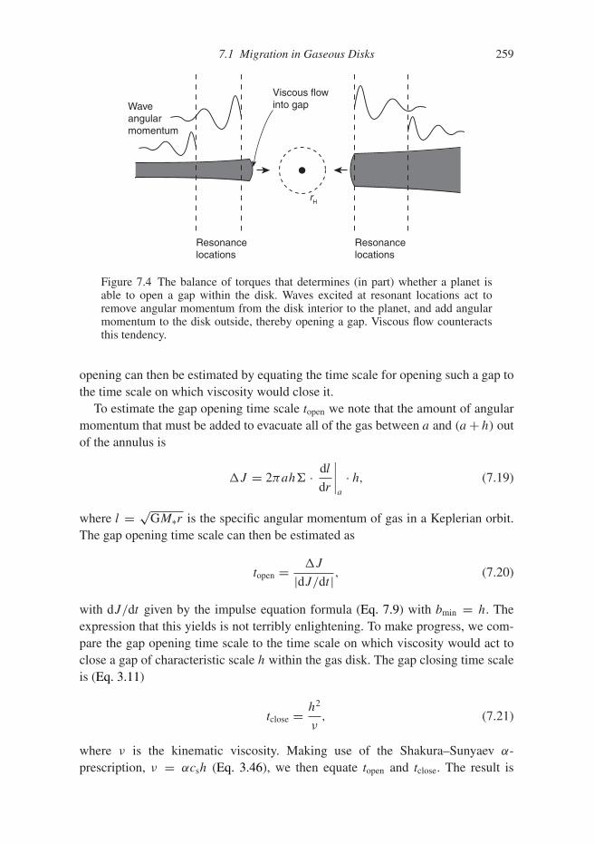
7.1 Migration in Gaseous Disks 259
Resonancelocations
Resonance locations
rH
Waveangularmomentum
Viscous flowinto gap
Figure 7.4 The balance of torques that determines (in part) whether a planet isable to open a gap within the disk. Waves excited at resonant locations act toremove angular momentum from the disk interior to the planet, and add angularmomentum to the disk outside, thereby opening a gap. Viscous flow counteractsthis tendency.
opening can then be estimated by equating the time scale for opening such a gap tothe time scale on which viscosity would close it.
To estimate the gap opening time scale topen we note that the amount of angularmomentum that must be added to evacuate all of the gas between a and (a + h) outof the annulus is
�J = 2πah� · dl
dr
∣∣∣∣a
· h, (7.19)
where l = √GM∗r is the specific angular momentum of gas in a Keplerian orbit.
The gap opening time scale can then be estimated as
topen = �J
|dJ/dt |, (7.20)
with dJ/dt given by the impulse equation formula (Eq. 7.9) with bmin = h. Theexpression that this yields is not terribly enlightening. To make progress, we com-pare the gap opening time scale to the time scale on which viscosity would act toclose a gap of characteristic scale h within the gas disk. The gap closing time scaleis (Eq. 3.11)
tclose = h2
ν, (7.21)
where ν is the kinematic viscosity. Making use of the Shakura–Sunyaev α-prescription, ν = αcsh (Eq. 3.46), we then equate topen and tclose. The result is

260 Early Evolution of Planetary Systems
an estimate for the critical mass ratio q ≡ Mp/M∗ between the planet and the starabove which a gap can be opened:
qcrit �(
27π
8
)1/2 (h
r
)5/2
α1/2. (7.22)
In this expression (h/r) is to be interpreted as the geometric thickness thatthe disk would have in the absence of the planet. For typical disk parameters(α = 10−3,h/r = 0.05) we obtain
qcrit � 6 × 10⁻⁵, (7.23)
which suggests that planets of Saturn mass orbiting solar mass stars should be ableto open gaps. The gap opening mass has no explicit dependence on the disk surfacedensity, but varies strongly with h/r .
An additional consideration is whether a two-dimensional treatment of planet–disk interaction is adequate to study gap opening, or whether three-dimensionalstudies are necessary. (The argument above is essentially two-dimensional.) A two-dimensional analysis can be justified if the Hill sphere (Eq. 5.15) of the planet islarger than the scale-height of the disk,
rH>∼ h. (7.24)
This will be true if the mass ratio exceeds
qcrit>∼ 3
(h
r
)3
, (7.25)
which evaluates to qcrit ≈ 4 × 10⁻⁴ for fiducial disk parameters. The similarityof this number to the threshold gap-opening mass implies that although two-dimensional models are useful, three-dimensional simulations are often necessaryfor accurate studies of the gap-opening process.
An analytic estimate for the depth of the gap created by a planet can be derivedusing an approach quite similar to that used to determine the gap-opening criterion.Following Kanagawa et al. (2015), we first note that the radial flux of angularmomentum through the disk can be written as the sum of an advective and viscouspiece (Eq. 3.5),
FJ (r) = −r2�M − 2πr3ν�d�
dr. (7.26)
We assume that the planet orbits at r = a, and that the gap extends out to r = r+.If the gap is wide enough that essentially all of the one-side Lindblad torque isexerted on gas within the gap, then the angular momentum flux at the outer gapedge is equal to the sum of that passing through the disk at the location of theplanet plus the planetary torque:
FJ (r+) = FJ (a) + �LB,1. (7.27)

7.1 Migration in Gaseous Disks 261
The impulse approximation yields the scalings of the one-sided planetary torque,but for a numerical estimate we use a better calculation, based on a sum over exte-rior Lindblad resonances, which gives (Tanaka et al., 2002; Kanagawa et al., 2015)
�LB,1 = 0.12π
(Mp
M∗
)2 (h
r
)−3
a4�gap�2K . (7.28)
We now assume that although the gap is wide enough to absorb all of the one-sided torque, it is narrow enough that r+ ≈ a and �K(r+) ≈ �K(a). In thatcase, FJ (r+) and FJ (a) differ only via the second term in Eq. (7.26). Noting thatd�/dr = −(3/2)(�K/r) for a Keplerian disk, and using the alpha prescription towrite ν =αh2�K, Eq. (7.26) becomes
3πa4α
(h
r
)2
�2K�disk = 3πa4α
(h
r
)2
�2K�gap
+ 0.12π
(Mp
M∗
)2 (h
r
)−3
a4�gap�2K . (7.29)
Simplifying and rearranging we get an expression for the gap depth,
�gap
�disk= 1
1 + 0.04K, (7.30)
where the power of a planet to open a gap is expressed via the parameter,
K ≡(
Mp
M∗
)2 (h
r
)−5
α−1. (7.31)
Making a somewhat arbitrary definition that a gap “opens” when �gap/�disk ≤ 0.5,we find that the threshold mass ratio needed to open a gap has the same scalingderived before, qcrit ∝ (h/r)5/2α1/2. This is to be expected as the physical argumentis almost the same. The numerical value of qcrit is slightly larger. The more refinedanalysis, however, does give us something new – the predicted depth of the gapover the transition between the Type 1 and Type 2 regimes. Numerical simulationscollated by Kanagawa et al. (2015) show reasonable agreement with the analyticprediction.
7.1.6 Coupled Planet–Disk Evolution
Determining the migration history of a planet due to gas disk torques requires awell-specified model for the protoplanetary disk, which includes at a minimumthe profiles of surface density, temperature, viscosity, and thermal diffusivity(together with any time dependence of these quantities). In the Type I regime,torque formulae can then be used to compute the rate of migration as a function ofsemi-major axis and planet mass within the given disk model. Examples of suchmigration maps are given by Bitsch et al. (2015). The results are quite sensitive to
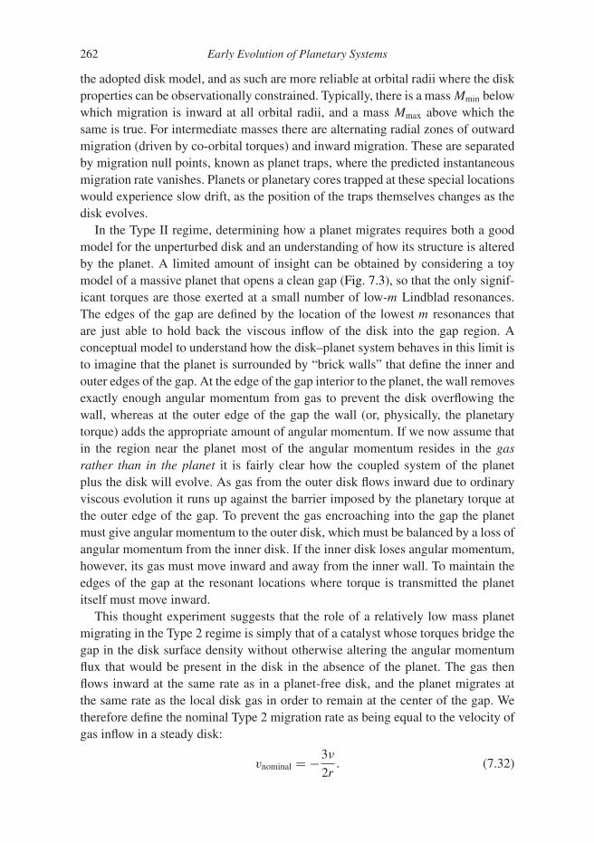
262 Early Evolution of Planetary Systems
the adopted disk model, and as such are more reliable at orbital radii where the diskproperties can be observationally constrained. Typically, there is a mass Mmin belowwhich migration is inward at all orbital radii, and a mass Mmax above which thesame is true. For intermediate masses there are alternating radial zones of outwardmigration (driven by co-orbital torques) and inward migration. These are separatedby migration null points, known as planet traps, where the predicted instantaneousmigration rate vanishes. Planets or planetary cores trapped at these special locationswould experience slow drift, as the position of the traps themselves changes as thedisk evolves.
In the Type II regime, determining how a planet migrates requires both a goodmodel for the unperturbed disk and an understanding of how its structure is alteredby the planet. A limited amount of insight can be obtained by considering a toymodel of a massive planet that opens a clean gap (Fig. 7.3), so that the only signif-icant torques are those exerted at a small number of low-m Lindblad resonances.The edges of the gap are defined by the location of the lowest m resonances thatare just able to hold back the viscous inflow of the disk into the gap region. Aconceptual model to understand how the disk–planet system behaves in this limit isto imagine that the planet is surrounded by “brick walls” that define the inner andouter edges of the gap. At the edge of the gap interior to the planet, the wall removesexactly enough angular momentum from gas to prevent the disk overflowing thewall, whereas at the outer edge of the gap the wall (or, physically, the planetarytorque) adds the appropriate amount of angular momentum. If we now assume thatin the region near the planet most of the angular momentum resides in the gasrather than in the planet it is fairly clear how the coupled system of the planetplus the disk will evolve. As gas from the outer disk flows inward due to ordinaryviscous evolution it runs up against the barrier imposed by the planetary torque atthe outer edge of the gap. To prevent the gas encroaching into the gap the planetmust give angular momentum to the outer disk, which must be balanced by a loss ofangular momentum from the inner disk. If the inner disk loses angular momentum,however, its gas must move inward and away from the inner wall. To maintain theedges of the gap at the resonant locations where torque is transmitted the planetitself must move inward.
This thought experiment suggests that the role of a relatively low mass planetmigrating in the Type 2 regime is simply that of a catalyst whose torques bridge thegap in the disk surface density without otherwise altering the angular momentumflux that would be present in the disk in the absence of the planet. The gas thenflows inward at the same rate as in a planet-free disk, and the planet migrates atthe same rate as the local disk gas in order to remain at the center of the gap. Wetherefore define the nominal Type 2 migration rate as being equal to the velocity ofgas inflow in a steady disk:
vnominal = −3ν
2r. (7.32)
7.1 Migration in Gaseous Disks 263
Using the α-prescription once more we obtain
vnominal = −3
2α
(h
r
)2
vK, (7.33)
where vK is the Keplerian orbital velocity. The speed of Type 2 migration dependsupon poorly known disk parameters (in particular, it depends linearly on theefficiency of angular momentum transport as parameterized via α) but it isgenerically rather rapid. The coupled evolution of a massive planet embeddedwithin an evolving disk can be approximately modeled with straightforwardgeneralizations of the one-dimensional disk evolution equation discussed inSection 3.2 (Lin & Papaloizou, 1986). Figure 7.5 shows an example of such acalculation, which predicts migration time scales from 5 AU of the order of 105 yr.One should note that although migration is always inward in a steady disk of largeradial extent, the argument actually implies only that the planet ought to track the
(
)
(
)
( )
( )
Planet
Figure 7.5 Predicted Type 2 migration of a 1 MJ planet formed within an evolvingprotoplanetary disk at 5 AU, based on an approximate one-dimensional treatmentof the interaction (Armitage et al., 2002). The calculation assumes that there is nomass flow across the gap, and that no mass is accreted by the planet. The upperpanel shows the disk surface density as a function of radius at three differentepochs, while the lower panel shows the evolution of the planetary semi-majoraxis. The model assumes that the planet formed at an early epoch while the gasdisk was still massive. The planet migrates inward within a gap on a short timescale, reaching small radii after approximately 105 yr.

264 Early Evolution of Planetary Systems
local motion of the surrounding gas. A planet that forms near the outer edge ofa disk that is expanding viscously would therefore migrate with the gas to largerorbital radii (Veras & Armitage, 2004).
The actual Type 2 migration is expected to differ from the nominal rate due toat least two effects. Migration will slow if the local disk mass (∼ πa2�) is smallcompared to the planet mass, as a low mass disk is unable to transport away angularmomentum at the high rate that would be needed to sustain the nominal speed. Moregenerally, however, the rate of Type 2 migration is modified because simulationsshow that the edges of planet-carved gaps are rather porous dams. Gas can flowacross the gap, violating the assumption of no flow that anchored the estimate ofthe nominal migration rate, and can be accreted by the planet, directly altering itsangular momentum. Papers by Duffell et al. (2014), Durmann and Kley (2015),Kanagawa et al. (2018), and Robert et al. (2018) report simulation results thatquantify the magnitude of the discrepancy.
7.1.7 Eccentricity Evolution
Up to now we have focused on the evolution of the semi-major axes of planetsexperiencing gas disk migration. An important question is whether eccentricity canbe excited as a consequence of planet–disk interactions during Type 2 migration,as this could be a mechanism able to explain the observed non-zero eccentricitiesof many giant extrasolar planets. Eccentricity evolution can be investigated withinthe same resonant framework used to compute the net torque, by evaluating thenet damping or excitation of planetary eccentricity that results from the interactionof a slightly eccentric planet with the disk at all significant resonant locations(Goldreich & Tremaine, 1980). Table 7.1 lists the nine most important resonances,3
along with the sign of the eccentricity change they induce on an embedded planet(Goldreich & Sari, 2003; Ogilvie & Lubow, 2003; Masset & Ogilvie, 2004). Theinteraction at some resonances excites eccentricity, while that at others dampsit. For a massive planet that clears a gap (so that the three co-orbital resonanceslisted in the table play no role) the balance between excitation and damping at theremaining resonances is delicate, with damping winning by only a narrow margin.This conclusion could be reversed in a number of ways, most of which involvesuppressing the damping effect of the first-order co-rotation resonances by at leasta small amount. This suppression could occur if the planet clears a very wide gap (ashappens for binary stars, Artymowicz et al., 1991), or if the co-rotation resonancesare intrinsically slightly weaker due to saturation at less than the nominal strength(Goldreich & Sari, 2003; Ogilvie & Lubow, 2003).
3 The nomenclature of “fast” and “slow” denotes resonances that occur where the pattern speed is either faster orslower than the planet’s orbital frequency.

7.2 Secular and Resonant Evolution 265
Table 7.1 List of the principal and first-order Lindblad andco-rotation resonances, together with their effect on the eccentricityof an embedded giant planet (after Masset & Ogilvie, 2004).
Resonance (r/a)−2/3 Effect on e
Principal OLR m/(m + 1) excitePrincipal ILR m/(m − 1) dampCo-orbital CR 1 unclearFast first-order OLR 1 dampFast first-order ILR (m + 1)/(m − 1) exciteFast first-order CR (m + 1)/m dampSlow first-order OLR (m − 1)/(m + 1) exciteSlow first-order ILR 1 dampSlow first-order CR (m − 1)/m damp
Numerical simulations confirm the analytic prediction that substantial eccentric-ities can be excited for very massive planets or brown dwarfs (with masses Mp
>∼ 5–20 MJ) that create deep and wide gaps. In these circumstances eccentricity is exciteddue to the dominant influence of the 3:1 exterior Lindblad resonance (Papaloizouet al., 2001). Lower mass giant planets can also experience eccentricity growth, butthe maximum eccentricity is limited. Simulations suggest that the limit may be ofthe order of e ∼ (h/r), and certainly cannot exceed a limit set by the requirementthat the apocenter of the orbit remains within the gap e ∼ 0.1 (D’Angelo et al., 2006;Duffell & Chiang, 2015; Ragusa et al, 2017).
7.2 Secular and Resonant Evolution
In our survey of the Solar System (Section 1.1) we noted that a resonance occurswhen there is a near-exact commensurability among the characteristic frequenciesof one or more bodies. The use of the term “characteristic frequency” is deliberatelyvague, since it must encompass a wide variety of possibilities that include the orbitalfrequency, the spin frequency of a planet’s rotation, the precession frequency of theorbit, and more. We can start, however, by considering the simplest case where thecommensurability is between the orbital frequencies (or periods) of two planets oncircular orbits. We have already noted (Eq. 1.3, here expressed in an equivalentform) that the condition for resonance can be written as
Pin
Pout� p
p + q, (7.34)
where Pin and Pout are the orbital periods of the two planets and p and q are integers.The definition, of course, raises the immediate question of what is meant by theapproximate equality sign. How close do the two planets have to be to the exactcommensurability for them to be as a practical matter “in resonance”? To address

266 Early Evolution of Planetary Systems
this we first consider how gravitational perturbations affect a system that is closeto an exact commensurability, and then sketch out how to mathematically definewhether a given system is resonant or not.
7.2.1 Physics of an Eccentric Mean-Motion Resonance
The essential physics of mean-motion resonances resonances can be understood byconsidering the simple model system shown in Fig. 7.6 (Peale, 1976). A massiveplanet min with a circular orbit has a low mass outer companion mout with a signif-icantly eccentric orbit. We assume that the orbital periods of the planets (obtainedby fitting Keplerian orbits to the instantaneous position and velocity data) are closeto an integer ratio, and examine how the small perturbations the inner planet exertson the outer affect the evolution.
At conjunction (when the two planets line up on one side of the star) and at oppo-sition (when they line up with the star in between) the gravitational perturbationmin exerts on mout is radial, and does not act to change the angular momentum ofthe outer body’s orbit. During the interval between opposition and conjunction theouter body is ahead of the inner one along its orbit, and the tangential componentof the mutual gravitational force acts to remove angular momentum from mout.Conversely, between conjunction and the next opposition the interactions works toadd angular momentum to mout. It is easy to see that if conjunctions occur at either
PericenterApocenter
Eccentric outer planet mout << min
Circular innerplanet mass min
Conjunctionat point A
Conjunctionat point B
Closer planets,larger force
More distant planets,smaller force
L > 0n < 0
..
L < 0n > 0
..
Conjunctionat point C
Conjunctionat point D
Star
Figure 7.6 Illustration, after Peale (1976), of how gravitational perturbations actto keep two planets with nearly commensurate orbital periods in resonance. Forsimplicity, the model system consists of a massive inner body on a circular orbittogether with a low mass outer body on an eccentric orbit.

7.2 Secular and Resonant Evolution 267
pericenter or apocenter the angular momentum gaining and angular momentumlosing phases are symmetric, and there is no net transfer of angular momentumbetween the bodies.
The symmetry is broken if conjunctions occur at a general point along the orbit.Suppose, for example, that a conjunction occurs at point A in Fig. 7.6. Because thetrajectories of the planets are diverging as they pass through conjunction (due tothe eccentric orbit of mout), the gravitational perturbation on mout just prior to theconjunction is stronger than that just afterwards. Additionally, the angular velocityof mout is slowing down as it passes through point A moving toward apocenter,so there is also more time for the perturbation to act prior to conjunction thanthere is afterwards. Both effects work in the same sense, such that the interaction(averaged between one conjunction and the next) acts to remove angular momentumL from mout. A similar argument shows that angular momentum is added to mout ifconjunctions occur instead at point B.
A planet that loses angular momentum moves to an orbit with a shorter periodP and a larger mean motion n ≡ 2π/P . This means that a conjunction that occursat point A will be followed by a conjunction that occurs closer to apocenter. Thesame is true for a conjunction at point B. We say that the point of conjunctionlibrates (oscillates) stably about apocenter, maintaining the system in resonanceeven though the instantaneous orbital periods of the planets are not usually exactlycommensurate. Stable libration remains possible even if we include the effect oforbital precession which is also driven by the mutual gravitational perturbationsbetween the planets.
Exactly the same methods can be applied to analyze the stability of conjunctionsthat occur at points C and D, near pericenter. Both are driven away from pericenter,which is an unstable equilibrium point of the system.
The scenario that we have analyzed here applies to a number of Solar Systemresonances, including some between the satellites of Saturn and between Jupiterand non-co-orbital asteroids. It is not however general, and physically differentoutcomes are possible if different assumptions are adopted. For example, stablelibration at pericenter as well as apocenter is possible if the eccentricity of theouter orbit is small. Peale (1976) provides an elementary explanation of this limit,following the same line of reasoning that we have applied to the high eccentricitycase.
7.2.2 Example Definition of a Resonance
The physical description of resonance given above makes it fairly clear how todefine the condition of being in resonance mathematically. Let us first assume thattwo planets are in exact resonance and rewrite Eq. (7.34) in terms of the meanmotions of the planets:
nout
nin= p
p + q. (7.35)

268 Early Evolution of Planetary Systems
If we ignore any perturbations between the planets, the angle λ between the radiusvector to one of the planets and a reference direction advances linearly with time.Defining t = 0 and λ = 0 to coincide with a moment when the two planets are inconjunction, we have that
λin = nint, (7.36)λout = noutt, (7.37)
and the resonance condition becomes
(p + q)λout = pλin. (7.38)
Finally, we can define a resonant argument
θ = (p + q)λout − pλin, (7.39)
which will evidently remain zero for all time if the planets are in exact resonance.For planets on general circular orbits, on the other hand, λin and λout still advancelinearly with time, but no small p and q can be found so that θ remains a constant.Sampled at random intervals, in fact, θ takes on all values in the range [0,2π ]. It isthis basic distinction that furnishes a definition of what it means for two planetsto be in resonance. A resonance occurs when one or more resonant arguments isbounded (though it need not be exactly constant), while there is no resonance if theargument takes on all possible values.
In more detail, we follow Murray and Dermott (1999) and analyze the conditionsfor resonance within the context of the circular restricted three-body problem. Wefirst review some nomenclature for eccentric orbits. The mean anomaly is given by
M = n(t − tperi), (7.40)
where tperi is the time of pericenter passage. The mean longitude is
λ = M + �, (7.41)
where � is the longitude of pericenter. We now consider the condition for exactresonance between a planet on a circular orbit (ein = 0) and a low mass body onan eccentric orbit (eout �= 0). The potential experienced by the low mass body isnot quite Keplerian, but to a good approximation we can assume that the orbit isan instantaneous Keplerian orbit whose longitude of pericenter varies with time atsome rate �out �= 0. Working in a frame that rotates along with the drift in thelongitude of pericenter of the outer body, the condition for exact resonance is
nout − �out
nin − �out= p
p + q, (7.42)
and the resonant argument is
θ = (p + q)λout − pλin − q�out. (7.43)
7.2 Secular and Resonant Evolution 269
Both the physical argument given already and a mathematical treatment show thatif the system is close to the exact resonance, perturbations between the bodiesact such as to keep θ bounded even if the instantaneous periods are not exactlycommensurable. We say that the system is:
• In resonance if θ librates, by which we mean that the resonant argument may betime dependent but varies only across some limited range of angles.
• Out of resonance if θ circulates, taking on all values between 0 and 2π .
In fact for this model problem it can be shown that the behavior of θ over timeis remarkably simple, and the angle oscillates in a manner that is mathematicallyidentical to that of a pendulum:
d2θ
dt2+ ω2
0 sin θ = 0. (7.44)
The oscillation frequency ω0 is known in this context as the libration frequency, andthe corresponding time scale,
tlib ≡ 2π
ω0, (7.45)
as the libration time scale. The final basic quantity of interest is the range of semi-major axis values for which θ librates rather than circulates. This quantity is calledthe width of the resonance. Although one cannot state any simple general formulaefor these quantities, it is possible to derive analytic estimates of the widths andlibration time scales for particular resonances that are of interest (see e.g. Holman& Murray, 1996 for a concise description of the method).
Our focus up to this point on mean-motion resonances should not blind thereader into forgetting that a planetary system has a large number of characteristicfrequencies, and as a consequence the number of possible resonant arguments isvery large. Other types of resonance that are of interest include:
• Secular resonances, where the commensurable frequencies involve the slow pre-cession of the longitude of pericenter or the longitude of the ascending node dueto mutual interactions between the bodies. A simple example of a secular resonantargument is θ = �in − �out.
• Resonances that involve inclination.
• Three-body resonances. A Solar System example is the three-body resonanceinvolving Jupiter, Saturn, and Uranus: nJ − 7nU = 5nSat − 2nJ.
• So-called secondary resonances, which include cases where the libration fre-quency of two planets in resonance is itself commensurable with some otherfrequency of the system.
Although in the Solar System there are no simple mean-motion resonances amongthe planets, a plethora of these weaker resonances are nonetheless believed to haveimportant dynamical effects. In particular, spatial overlap of different resonances is
270 Early Evolution of Planetary Systems
the accepted explanation for the apparent presence of chaos in the motion of theplanets. The review by Lecar et al. (2001) provides a good starting point for thereader who wishes to explore this intricate subject in more detail.
7.2.3 Resonant Capture
Since resonances have finite widths, there is some probability that two planets ina randomly assembled planetary system will happen to find themselves in a mean-motion resonance. Even a cursory inspection of data on the Solar System, however,convinces one of the need for a causal rather than a probabilistic explanation forentry into resonance. Chiang et al. (2007), for example, find that in excess of 20%of Kuiper Belt Objects with well-determined orbits are in mean-motion resonanceswith Neptune, with the 3:2 resonance occupied by Pluto being the most heavilypopulated. Among satellites too there are numerous known resonances, of whichthe most striking is the 4:2:1 resonance that involves three of the Galilean satel-lites of Jupiter – Io, Europa, and Ganymede. Mean-motion resonances betweenplanets themselves also appear to be common among extrasolar planetary systems.Resonances have been securely identified in approximately 20% of known multipleplanet systems, and there are additional systems that are plausibly but not yetprovably in resonance.4 One well-known example is the GJ 876 system (Marcyet al., 2001), in which two massive planets orbit in a 2:1 resonance with orbitperiods of approximately one and two months. For this system both of the lowest-order mean motion resonant arguments,
θ1 = λin − 2λout + �in, (7.46)
θ2 = λin − 2λout + �out, (7.47)
and the secular resonant argument,
θ3 = �in − �out, (7.48)
librate about zero degrees (Lee & Peale, 2001).The likely origin of most of these mean-motion resonances lies in the phe-
nomenon of resonant capture, which was first studied for spin–orbit resonances(Goldreich & Peale, 1966) and subsequently developed to explain resonancesamong planetary satellites (Sinclair, 1972; Yoder, 1979; Borderies & Goldreich,1984). Resonant capture is possible when two bodies are driven toward resonance(i.e. their orbits converge) by the application of a (generally weak) external force –which could arise due to tidal effects on planetary satellites or torques from the
4 Identifying resonances in extrasolar planetary systems is generally difficult because in many cases the orbitalsolutions are of limited precision. Making an accurate statistical statement as to the true fraction of resonantplanetary systems is even harder, because the selection function for detecting two planets of given masses willgenerally differ depending upon whether they are in a resonance or not.

7.2 Secular and Resonant Evolution 271
gas disk in the case of extrasolar planets. As the bodies approach and then enterthe resonance there is a secular exchange of angular momentum between them thatacts so as to maintain the resonance despite the ongoing external forcing that wouldotherwise result in exit from the resonance. In the case of two planets whose orbitsconverge because the outer planet is subject to a torque causing inward migration,for example, the resonant coupling acts to remove angular momentum from theinner planet so that the two bodies move inward in lockstep. A heuristic (but stillquite intricate) description of the dynamics that results in this angular momentumtransfer is given by Peale (1976). An important general result of the theory is thatcapture can occur only for converging orbits. Two bodies whose orbits diverge suchthat they approach and enter a resonance still experience an increased strength ofinteraction – which may lead to significant excitation of eccentricity – but cannotbe captured into resonance according to the classical theory.
Even when it is possible (in the case of converging orbits) capture is generally aprobabilistic phenomenon whose likelihood depends (in part) upon the relationshipbetween the libration time scale tlib and the time scale on which the external forcingwould result in resonance crossing if capture did not occur:
tcross = �ares
|ain − aout| . (7.49)
Here �ares represents the width of the resonance under consideration. If tcross � tlib
then capture is guaranteed provided that the eccentricity of the body being capturedis below some limit, while for faster crossing the probability of capture will dependupon the eccentricity, the rate of convergence of the orbit, and the particular res-onance being encountered. Explicit expressions for the maximum drift rates thatpermit capture can be found in Quillen (2006, and references therein).
Resonant capture is a particularly appealing explanation for resonant extrasolarplanets in short-period orbits, whose small semi-major axes provide circumstantialevidence for the existence of migration torques that could have both shrunk theorbits and driven the planets into resonance. Figure 7.7 shows a numerical calcula-tion of resonant capture in a coplanar system of two Jupiter mass planets, where theouter planet is driven toward the inner one under the action of an external torque.For this choice of parameters capture occurs into the 2:1 resonance, which is thenmaintained as the orbits continue to shrink. Once in resonance, further decay of thesemi-major axes of the planets is accompanied by growth of the eccentricity, thoughthis may be damped (at least partially) by the interaction of the planets with the gasdisk. Although existing theory is not fully predictive – in particular planets migrat-ing through a turbulent gas disk can diffuse out of the resonance due to randomvariability in the torques they experience (Murray-Clay & Chiang, 2006; Adams etal., 2008) – resonant capture is at least qualitatively consistent with the observationof a significant population of extrasolar planets in mean-motion resonances.

272 Early Evolution of Planetary Systems
( )
()
Outer planet
Inner planet
Figure 7.7 Numerical example of resonant capture in a coplanar system of twoinitially well-separated Jupiter mass planets. For illustrative purposes the outerplanet is subjected to a fictitious drag force which results in steady decay of itssemi-major axis. The inner planet is almost unperturbed until the planets encountertheir mutual 2:1 mean-motion resonance, at which point capture occurs and thetwo planets move inward in lockstep.
7.2.4 Kozai–Lidov Dynamics
Kozai–Lidov dynamics is a quite different type of resonant behavior that is impli-cated in the evolution (and possibly formation) of some extrasolar planetary sys-tems. The simplest system that exhibits the characteristic Kozai–Lidov behavioris a hierarchical triple system, in which a massive outer binary companion per-turbs a low mass body on an inclined orbit closer in. The dynamics of this setupwas analyzed by Mikhail Lidov, in the context of the motion of artificial satellitesaround the Earth under the perturbation of external bodies, and by Yoshihide Kozai,in the context of the motion of high inclination asteroids perturbed by Jupiter(Lidov, 1962; Kozai, 1962).5 For the model system that consists of a low massbody orbiting well interior to a massive perturber on a highly inclined orbit theresonant argument is simply the argument of pericenter of the inner body itself.
The interest in this particular resonance derives from the very unusual evolutionthat occurs when the resonance is active. The simplest situation to analyze (and alsothe one most relevant for extrasolar planetary systems) is that shown in Fig. 7.8. Aplanet of mass Mp and semi-major axis ain orbits the primary star (mass M∗) of abinary system. The secondary star of the binary system has mass Ms, semi-majoraxis as, and eccentricity es, and orbits in a plane inclined to that of the planet by anangle i. Triple systems of this kind are typically only stable if they are hierarchical(i.e. the outer binary has a much larger orbit than that of the inner binary, which ishere the planet), so we consider the limit in which
5 Both of these now celebrated papers languished in relative obscurity for more than 30 years.
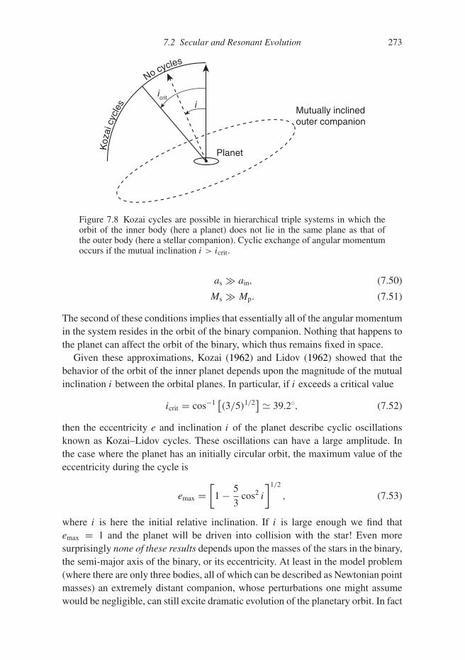
7.2 Secular and Resonant Evolution 273
Koz
aicy
cles
No cycles
iicrit
Planet
Mutually inclinedouter companion
Figure 7.8 Kozai cycles are possible in hierarchical triple systems in which theorbit of the inner body (here a planet) does not lie in the same plane as that ofthe outer body (here a stellar companion). Cyclic exchange of angular momentumoccurs if the mutual inclination i > icrit.
as � ain, (7.50)
Ms � Mp. (7.51)
The second of these conditions implies that essentially all of the angular momentumin the system resides in the orbit of the binary companion. Nothing that happens tothe planet can affect the orbit of the binary, which thus remains fixed in space.
Given these approximations, Kozai (1962) and Lidov (1962) showed that thebehavior of the orbit of the inner planet depends upon the magnitude of the mutualinclination i between the orbital planes. In particular, if i exceeds a critical value
icrit = cos−1[(3/5)1/2
] � 39.2◦, (7.52)
then the eccentricity e and inclination i of the planet describe cyclic oscillationsknown as Kozai–Lidov cycles. These oscillations can have a large amplitude. Inthe case where the planet has an initially circular orbit, the maximum value of theeccentricity during the cycle is
emax =[
1 − 5
3cos2 i
]1/2
, (7.53)
where i is here the initial relative inclination. If i is large enough we find thatemax = 1 and the planet will be driven into collision with the star! Even moresurprisingly none of these results depends upon the masses of the stars in the binary,the semi-major axis of the binary, or its eccentricity. At least in the model problem(where there are only three bodies, all of which can be described as Newtonian pointmasses) an extremely distant companion, whose perturbations one might assumewould be negligible, can still excite dramatic evolution of the planetary orbit. In fact
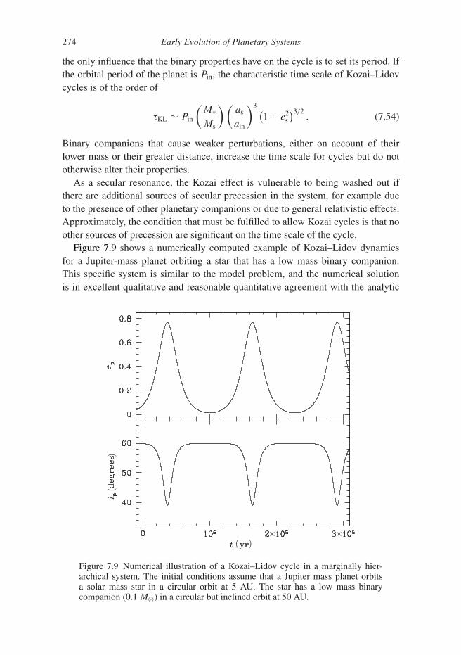
274 Early Evolution of Planetary Systems
the only influence that the binary properties have on the cycle is to set its period. Ifthe orbital period of the planet is Pin, the characteristic time scale of Kozai–Lidovcycles is of the order of
τKL ∼ Pin
(M∗Ms
)(as
ain
)3 (1 − e2
s
)3/2. (7.54)
Binary companions that cause weaker perturbations, either on account of theirlower mass or their greater distance, increase the time scale for cycles but do nototherwise alter their properties.
As a secular resonance, the Kozai effect is vulnerable to being washed out ifthere are additional sources of secular precession in the system, for example dueto the presence of other planetary companions or due to general relativistic effects.Approximately, the condition that must be fulfilled to allow Kozai cycles is that noother sources of precession are significant on the time scale of the cycle.
Figure 7.9 shows a numerically computed example of Kozai–Lidov dynamicsfor a Jupiter-mass planet orbiting a star that has a low mass binary companion.This specific system is similar to the model problem, and the numerical solutionis in excellent qualitative and reasonable quantitative agreement with the analytic
( )
(
)
Figure 7.9 Numerical illustration of a Kozai–Lidov cycle in a marginally hier-archical system. The initial conditions assume that a Jupiter mass planet orbitsa solar mass star in a circular orbit at 5 AU. The star has a low mass binarycompanion (0.1 M�) in a circular but inclined orbit at 50 AU.

7.2 Secular and Resonant Evolution 275
theory. It is possible to relax the restrictions of the original analytic theory, andconsider situations where the orbiting bodies both have non-negligible mass, orwhere the outer perturber starts on an eccentric orbit. The dynamics in this moregeneral case still permits large changes to the eccentricity and inclination of theinner body, but there are qualitative differences, including the possibility for theinclination of the inner body’s orbit to switch from prograde to retrograde (for areview, see Naoz, 2016).
From a theoretical perspective one would have to be dismayed if such a beautifuldynamical phenomenon remained an academic curiosity devoid of widespreadapplication in nature. Early applications of Kozai–Lidov dynamics to extrasolarplanetary systems focused on systems in known binaries with properties that couldplausibly drive Kozai–Lidov cycles. The planet around 16 Cyg B is an example,and a strong argument can be made for the probable effectiveness of the mechanismin such specific cases (Holman et al., 1997).
Kozai–Lidov dynamics is also a channel that can potentially lead to the formationof hot Jupiters in orbits that are misaligned to the spin of their host stars, via a high-eccentricity tidal migration mechanism similar to that studied in the context of triplestellar systems (Eggleton & Kiseleva-Eggleton, 2001). Starting with a giant planeton a relatively wide orbit, Kozai–Lidov dynamics can generate large-amplitudeexcursions in eccentricity that lower the minimum pericenter distance ain(1 − emax)
to the point where tidal interactions with the star can act to shrink the orbit (Wu &Murray, 2003; Fabrycky & Tremaine, 2007). (Note that Kozai–Lidov dynamics onits own does not alter the semi-major axis.) The basic prediction of this model –that a significant fraction of hot Jupiters ought to have misaligned orbits – is borneout by the observations of the Rossiter–McLaughlin effect discussed in Chapter 1.Population studies suggest that a large fraction of the hot Jupiters that show largeprojected obliquities could feasibly form as a consequence of high-eccentricity tidalmigration (Naoz et al., 2012; Petrovich & Tremaine, 2016).
7.2.5 Secular Dynamics
A planetary system in which no mean-motion resonances significantly affect thedynamics can be studied in a secular approximation. Averaging over the orbitalmotion, the gravitational potential of a planet on an eccentric orbit can be repre-sented by a ring of matter whose mass per unit length is simply inversely pro-portional to the velocity of the planet at that point along its orbit. Two or moresuch rings, which may be eccentric and/or inclined with respect to each other, exertmutual gravitational torques, which cause the eccentricity and mutual inclination toevolve with time. The semi-major axis of each planet remains fixed under secularevolution.
The mathematical description of secular evolution, which in its simplest formis an approximation valid for small eccentricities, is known as Laplace–Lagrange

276 Early Evolution of Planetary Systems
theory (e.g. Murray & Dermott, 1999). Secular evolution conserves, to a goodapproximation, a quantity known as the angular momentum deficit (AMD). Fora system of planets with masses Mj , semi-major axes aj , eccentricities ej , andinclinations with respect to the invariable plane ij , the angular momentum deficit isdefined as,
AMD =∑
j
�j
(1 − cos ij
√1 − e2
j
), (7.55)
where
�j = M∗Mj
M∗ + Mj
√G(M∗ + Mj)aj . (7.56)
The angular momentum deficit is the difference between the angular momentum ofthe actual system and a reference system in which the planets have the same massesand semi-major axes, but zero eccentricity and no mutual inclinations.
The conservation of AMD has two significant consequences. If the AMD is lowenough, it may be possible to show that the orbits of planets in the system can nevercross, no matter how the AMD is apportioned among the planets. This argumentdoes not guarantee stability, because secular theory itself is only an approximationto the dynamics, but it provides a useful and easy to calculate stability metric(Laskar, 1997). Conversely, if the AMD is high enough (and the planet spacinglarge enough), it may be possible to place enough of the AMD in the innermostplanet to drive e → 1. Numerical simulations show that the secular evolution ofsystems of multiple planets can be chaotic, and if this is the case it is likely thatthe innermost planet will acquire most of the AMD of the whole system given onlyenough time. Secular chaos in the high AMD limit is another mechanism that canlead to high eccentricity tidal migration, and the formation of hot Jupiters (Wu &Lithwick, 2011).
7.3 Migration in Planetesimal Disks
A generic prediction of the core accretion model is that the time scale needed toassemble the core becomes longer in the outermost reaches of the protoplanetarydisk. If giant planets form via core accretion we would therefore expect that outsidea “giant planet zone” there ought to lie a region of debris that has been unableto form large bodies. This expectation is consistent with the fact that althoughplanetesimals formed in the Solar Nebula out to a distance of ≈50 AU (as evidencedby the presence of the Kuiper Belt) there are no large bodies beyond Neptune in theSolar System. Our main goal in this section is to assess the possible dynamicalinfluence that a disk of leftover debris (which we will dub a planetesimal disk, eventhough the bodies may have growth substantially by accretion or been destroyed bycollisions) can exert on the orbits of neighboring giant planets.
7.3 Migration in Planetesimal Disks 277
Our first task is to estimate the amount of mass that might plausibly be presentwithin a planetesimal disk in the outer region of a newly formed planetary system.This will depend upon the outer extent of the zone of giant planet formation (insidethis radius the bulk of the planetesimals presumably end up within planets) andupon the assumed profile of the solid component of the protoplanetary disk. If weassume that the planetesimal disk tracks the surface density of the solid componentof the minimum mass Solar Nebula6 (Eq. 1.6), the integrated mass between radii ofrin and rout is
Mdisk = 4π�0
(r
1/2out − r
1/2in
), (7.57)
where �0 defines the normalization (the fiducial value for the outer minimummass Solar Nebula corresponds to 30 g cm−2 at 1 AU). As we will note later,there is considerable evidence to suggest that the Solar System’s ice giants formedconsiderably closer to the Sun than their current locations. We therefore assumethat the zone of giant planet formation in the early Solar System extended out to20 AU, so that the disk of leftover debris ranged between 20 AU and 50 AU. Withthese parameters we estimate that
Mdisk � 40 M⊕. (7.58)
This estimate exceeds the observed mass of the present-day Kuiper Belt by morethan two orders of magnitude. For it to be even remotely correct, dynamical pro-cesses must have removed almost all of the primordial material at some point duringthe lifetime of the Solar System.
The existence of a substantial debris disk in the outer reaches of a planetarysystem provides a long-lived (compared to the gas disk) reservoir of mass andangular momentum that can drive migration of any planets that are able to interactwith it. Suppose, for example, that a planet of mass Mp orbiting interior to thedisk scatters a mass of planetesimals δm into shorter period orbits at smaller radii.Elementary considerations suggest that the resulting change in the planetary semi-major axis ought to be of the order of
δa
a∼ δm
Mp. (7.59)
Note that this cannot be the same process of small-angle scattering that we dis-cussed in the context of gas disk migration (Section 7.1) since the sense of migra-tion is reversed – we are imagining the planet to scatter planetesimals into lower
6 Although we have previously warned of the dangers of placing too much trust in the minimum mass SolarNebula profile, its use here is justifiable, since it is derived empirically from estimates of the mass of heavyelements within the planets. Given only weak assumptions (primarily that the planetesimal disk had acontinuous surface density distribution in the outer Solar System) it is reasonable to use it to estimate themass of planetesimals that did not form planets beyond the orbit of the last giant planet.

278 Early Evolution of Planetary Systems
angular momentum orbits and hence to migrate outward toward the exterior disk.For significant migration to occur we therefore require, at a minimum, that
Mp<∼ Mdisk. (7.60)
True gas giants with masses (typically) of hundreds of Earth masses are thereforerelatively impervious to planetesimal-driven migration, whereas this estimate sug-gests that lower mass ice giants such as Uranus and Neptune could suffer substantialmigration given the existence of planetesimal disks with plausible masses. There is,however, an obvious complication. Even if the total disk mass is large enough topermit migration, the mass of material that the planet is able to interact with at anyone time is much smaller. A planet migrating through a planetesimal disk may stall(or at least slow down dramatically) if the disk surface density is too small, sincethe planet will then scatter all of the bodies it is able to perturb without moving farenough to start interacting with a fresh population. This argument – which is a closecousin of the reasoning behind the existence of the isolation mass (Section 5.2.3) –suggests that not just the integrated disk mass but also the local surface density areimportant parameters that determine the behavior of planetesimal-driven migration.
An approximate analytic model for migration within planetesimal disks can bedeveloped by borrowing ideas from the more complete treatments given by Idaet al. (2000) and by Kirsh et al. (2009). We consider an asymmetric configurationin which a planet of mass Mp and orbital radius a lies just inside an exterior diskof planetesimals of surface density �p. At t = 0 there are no planetesimals atr < a. We assume that the planet migrates outward into the disk as a consequenceof scattering planetesimals inward on to lower angular momentum orbits, and thatits migration is fast enough that any individual planetesimal is scattered inward anddoes not then interact further with the planet.
An analysis of this model is straightforward. We first note that the planet will beable to perturb planetesimals strongly only within a radial zone whose width �r isof the order of the radius of the planet’s Hill sphere (cf. Section 5.1.2):
�r ≈(
Mp
3M∗
)1/3
a. (7.61)
The mass of planetesimals within this zone is
�m = 2πa�p�r . (7.62)
We now need to estimate the average change in the specific angular momentum of aplanetesimal that results from scattering. This can be calculated accurately, but fornow we simply assume that it is of the order of the difference in specific angularmomentum of circular orbits across the scattering zone. If this is the case, then onceall of the planetesimals within the scattering zone have encountered the planet theywill have collectively lost an amount of angular momentum

7.3 Migration in Planetesimal Disks 279
�J ≈ �mdl
dr
∣∣∣∣a
�r, (7.63)
where l = √GM∗r is the specific angular momentum for a circular orbit at dis-
tance r . The angular momentum lost by the planetesimals is gained by the planet,which (if it stays on a circular orbit) migrates outward a distance
�a ≈ 2πa�p�r2
Mp. (7.64)
For rapid migration to occur, �a must be large enough to move the planet into aregion of the disk stocked with as yet unperturbed planetesimals. Requiring that�a >∼ �r we obtain a condition on the planet mass
Mp<∼ 2πa�p�r . (7.65)
Fast planetesimal-driven migration requires that the planet mass be smaller than themass of planetesimals within a few Hill radii of the planet. One may observe againthat this behavior is the opposite of that predicted for Type 1 migration in a gasdisk, which becomes more rather than less efficient as the planet mass increases.
The rate of migration can be determined by estimating how long it takes for all ofthe planetesimals within the scattering zone to encounter the planet and be scatteredinward. The relevant time scale is that set by the shear across the scattering zone(Eq. 7.6):
�t ∼ 2
3
a
�rP, (7.66)
where P is the planetary orbital period. Combining this with the expression for thedistance that the planet moves (Eq. 7.64), we conclude that the migration rate in thefast regime will be
da
dt∼ a
P
πa2�p
M∗. (7.67)
Up to numerical factors of the order of unity this expression matches that derivedby Ida et al. (2000), and is in good agreement with numerical results. An interestingfeature of the result is that the migration of a low mass planet through a massiveplanetesimal disk occurs at a rate that is independent of the planet mass. Slower butstill substantial migration can occur for planets that are up to an order of magnitudemore massive than the rough limit defined by Eq. (7.65). Kirsh et al. (2009) providean empirical fit to numerical calculations of migration in the slow high-mass planetregime.
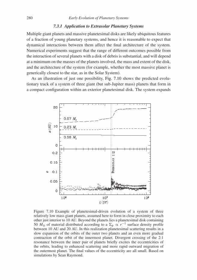
280 Early Evolution of Planetary Systems
7.3.1 Application to Extrasolar Planetary Systems
Multiple giant planets and massive planetesimal disks are likely ubiquitous featuresof a fraction of young planetary systems, and hence it is reasonable to expect thatdynamical interactions between them affect the final architecture of the system.Numerical experiments suggest that the range of different outcomes possible fromthe interaction of several planets with a disk of debris is substantial, and will dependat a minimum on the masses of the planets involved, the mass and extent of the disk,and the architecture of the system (for example, whether the most massive planet isgenerically closest to the star, as in the Solar System).
As an illustration of just one possibility, Fig. 7.10 shows the predicted evolu-tionary track of a system of three giant (but sub-Jupiter mass) planets that form ina compact configuration within an exterior planetesimal disk. The system expands
( )
()
Figure 7.10 Example of planetesimal-driven evolution of a system of threerelatively low mass giant planets, assumed here to form in close proximity to eachother just interior to 10 AU. Beyond the planets lies a planetesimal disk containing50 M⊕ of material distributed according to a �p ∝ r−1 surface density profilebetween 10 AU and 20 AU. In this realization planetesimal scattering results in aslow expansion of the orbits of the outer two planets and an even more gradualcontraction of the orbit of the innermost planet. Divergent crossing of the 2:1resonance between the inner pair of planets briefly excites the eccentricities ofthe orbits, leading to enhanced scattering and more rapid outward migration ofthe outermost planet. The final values of the eccentricity are all small. Based onsimulations by Sean Raymond.

7.4 Planetary System Stability 281
slowly as the planetesimal disk is depleted via scattering before experiencing anaccelerated phase of evolution that coincides with the eccentricity excitation accom-panying a 2:1 resonance crossing. Once the resonance has been crossed, furtherinteraction between the planets and the remaining disk material damps planetaryeccentricities to small values.
7.4 Planetary System Stability
In the guise of the stability of the Solar System the problem of planetary systemdynamics has a history dating back to Isaac Newton, who understood that the near-circular orbits of the planets were a special case whose survival was endangered bythe planet–planet forces required by his law of gravitation. Those forces are smallbut they work over a long time – billions of years in a modern understanding – andit is not obvious whether their effects ultimately average to zero or rather build upuntil they destabilize the system. Newton himself feared the worst. In his Opticks hewrote that “blind fate could never make all the planets move one and the same wayin concentric orbits, some inconsiderable irregularities excepted which may havearisen from the mutual actions of comets and planets upon one another, and whichwill be apt to increase, till this system wants a Reformation.” This was guessworkand it has taken three centuries of mathematical development to show that Newtonwas largely, though not entirely, wrong.
In a colloquial sense the fact that the Earth has sustained life for a substantialfraction of the age of the Solar System provides compelling evidence for the basicstability of at least our planetary system. Similarly, it would be shocking to discoverthat any known extrasolar planetary system (most of which are also billions ofyears old) was about to suffer some catastrophic event such as a planetary colli-sion or ejection. The interest in planetary system stability concerns not such grossquestions, but rather two substantially subtler aspects. One is the mathematicalquestion of whether (and if so when) it is possible to prove that an N-body systemis stable for all time, especially in the practically important case that the motionsof the bodies are chaotic and thus intrinsically unpredictable over sufficiently longtime scales. The second arises from the fact that nothing we have discussed aboutthe formation of planetary systems requires that the outcome will be a stable system.On the contrary, since planet formation plays out in a highly dissipative environ-ment – where either gas or planetesimal disks can frustrate the development ofslow-growing gravitational instabilities – it is plausible to imagine that the typicalplanetary system forms in what turns out to be a long-term unstable state. If this iscorrect, features such as the chaotic orbits of Solar System planets and the eccentricorbits of some extrasolar planets may be endpoints of the evolution of initiallyunstable planetary systems, and it is important to understand how unstable systemsevolve.

282 Early Evolution of Planetary Systems
7.4.1 Hill Stability
The trajectories of two point masses moving under Newtonian gravitational forcesare stable and well known: elliptical orbits if the bodies are gravitationally bound,and parabolae or hyperbolae otherwise. For systems of three or more bodies, on theother hand, no general closed form analytic solutions to the motion of the bodiesexist.7 Nonetheless, it is sometimes possible to demonstrate the stability of a systemof three bodies despite our ignorance of the actual trajectories, and although thestability criteria derived in this way are formally irrelevant for studies of more com-plex planetary systems they provide at least a framework for interpreting numericalresults.
The only example of three-body motion for which it is easy to derive an ana-lytic stability bound is the circular restricted three-body problem. We consider themotion of a test particle of negligible mass in the gravitational field of a circularstar–planet system, and work in a frame that co-rotates with the orbital motion ofthe planet at angular velocity �. We have already derived the equations describingthe motion of a test particle in this situation (the geometry is shown in Fig. 5.2 anddiscussed in Section 5.1.2). If the star and planet orbit in the (x,y) plane, then in aCartesian coordinate system in which the star and planet lie along the y = 0 line atx = −x∗ and x = xp we have
x − 2�y − �2x = −G
[M∗(x + x∗)
r3∗+ Mp(x − xp)
r3p
], (7.68)
y + 2�x − �2y = −G
[M∗r3∗
+ Mp
r3p
]y, (7.69)
z = −G
[M∗r3∗
+ Mp
r3p
]z. (7.70)
Here r∗ and rp are the instantaneous distances between the test particle and the starand planet. No assumptions have been made as to the masses of the star M∗ andplanet Mp.
The acceleration due to the centrifugal force can be subsumed into a pseudo-potential. Defining
U ≡ �2
2
(x2 + y2
) + GM∗r∗
+ GMp
rp, (7.71)
we obtain
x − 2�y = ∂U
∂x, (7.72)
7 The exceptions to this statement include fascinating mathematical curiosities, such as the “figure of eight”orbit for three equal mass bodies that was discovered by Chenciner and Montgomery (2000).

7.4 Planetary System Stability 283
y + 2�x = ∂U
∂y, (7.73)
z = ∂U
∂z. (7.74)
The Coriolis terms on the left-hand-side of the first two equations can be eliminatedby multiplying through by x,y, and z and adding. We then obtain
xx + yy + zz = x∂U
∂x+ y
∂U
∂y+ z
∂U
∂z, (7.75)
d
dt
(1
2x2 + 1
2y2 + 1
2z2
)= dU
dt. (7.76)
This equation integrates immediately to give
x2 + y2 + z2 = 2U − CJ, (7.77)
CJ = 2U − v2, (7.78)
where v is the velocity and CJ, called the Jacobi constant, is the arbitrary constantof integration. Note that CJ is an energy-like quantity that is a conserved quantityin the circular restricted three-body problem.
The existence of this integral of motion is important because it places limits onthe range of motion possible for the test particle. For a particle with a given initialposition and velocity we can use Eq. (7.78) to compute CJ, and hence to specifyzero-velocity surfaces, defined via
2U = CJ, (7.79)
which the particle can never cross. If the volume enclosed by one of the zero-velocity surfaces is finite, then a particle initially within that region is guaranteedto remain there for all time. By this argument one can prove stability of the systemwithout needing to derive an explicit form for the motion of the test particle.
The topology of the zero-velocity surfaces in the restricted three-body problemvaries according to the value of CJ. An example is shown in Fig. 7.11. In thisinstance the zero-velocity surfaces define three disjoint regions in the (x,y) plane,one corresponding to orbits around the star, one corresponding to orbits around theplanet, and one corresponding to orbits around the star–planet binary. A particle inany one of these states is stuck there – it cannot cross the forbidden zone betweenthe different regions to move into a different state.
Given these results a test particle’s orbit is guaranteed to be stable – in the sensethat it can never have a close encounter with the planet – if its Jacobi constant issuch that a zero-velocity surface lies between it and the planet. This condition canbe written in terms of a minimum orbital separation needed for stability. As anexample, consider a test particle in a circular orbit of radius aout in a system where

284 Early Evolution of Planetary Systems
Figure 7.11 Forbidden zones (dark regions) in the (x,y) plane in an example ofthe restricted three-body problem. For this particular choice of the Jacobi constantCJ, particles can orbit the star at small radii, the planet in a tight orbit, or the star–planet binary as a whole. The existence of zero-velocity surfaces, however, meansthat particles cannot be exchanged between these regions.
a planet has a circular orbit of radius ain. We define a dimensionless measure of theorbital separation � via
aout = ain(1 + �), (7.80)
and write the mass ratio between the planet and the star as
qin = Mp
M∗. (7.81)
Stability is then assured (irrespective of the initial difference in the longitudebetween test particle and planet) provided that
� > 2.4q1/3in . (7.82)
Since � is a measure of the orbital separation in units of (up to a small numericalfactor) Hill radii, this is a version of a result used in Section 5.2.2, where we arguedthat a planet will rapidly perturb small bodies on to crossing trajectories if theseparation is less than a few Hill radii. Here, we have demonstrated a more powerfulinverse result: if the separation is more than a few Hill radii, close encounters areabsolutely forbidden for all time.
Although Eq. (7.82) hints that the stability of a multiple planet system dependsupon the separation of the planets measured in units of Hill radii, nothing aboutthe above derivation gives us any right to expect that a formal proof of stabil-ity can be derived for a general two-planet system. Surprisingly, however, for

7.4 Planetary System Stability 285
qin, qout 1 it is possible to derive a sufficient condition for Hill stability8 that canbe applied to planets whose initial orbits have arbitrary eccentricity and inclination(Gladman, 1993; whose analysis draws on work by Marchal & Bozis, 1982).For two planets on initially circular coplanar orbits the system is Hill stable forseparations
� > 2 · 31/6 (qin + qout)1/3
+[
2 · 31/3 (qin + qout)2/3 − 11qin + 7qout
31/6(qin + qout)1/3
]+ · · · , (7.83)
which simplifies to lowest order in the mass ratios to
� > 2.4 (qin + qout)1/3 . (7.84)
This criterion reduces to that deduced earlier for the equivalent restricted three-body problem (Eq. 7.82). Among the more general results derived and quoted byGladman (1993) we note only the extension to the case where the planets have equalmasses (qin = qout = q) and initially small eccentricities,
� >
√8
3
(e2
in + e2out
) + 9q2/3, (7.85)
which, as with Eq. (7.84), is also valid only to lowest order in the masses.These stability criteria are formally only sufficient conditions for stability – they
guarantee that a planetary system with larger � is Hill stable but say nothing aboutwhether a more tightly packed system is actually unstable. For initially circularorbits (and only in that case), however, it is found empirically that the Hill limitis also a good general predictor of the onset of instability (with some exceptionssuch as systems with small � that are stable in resonant configurations). Anotherinteresting empirical finding is that two-planet systems that are Hill stable cannevertheless exhibit chaos, which is attributed to the overlap of multiple resonancesclose to (but beyond) the minimum separation needed for stability.
For systems of three or more planets there are no analytic guarantees of stability.The initial separation between planets in units of their mutual Hill radii,
rHill,m =(
Mp,i + Mp,i+1
3M∗
)1/3(ai + ai+1)
2, (7.86)
is still useful, however, as a guide to the time scale on which instability will resultin crossing orbits (Chambers et al., 1996). If we write the separation of the planetsin the form
8 As in the circular restricted three-body problem, a system that is “stable” by this criterion is guaranteed to befree of close encounters between the planets for all time. This is not quite the common-sense definition ofstability, since it leaves open the loophole that one planet might become unbound from the system via thecumulative action of many distant, weak encounters. A stronger definition of stability, known as Lagrangestability, requires that both planets remain bound. Lagrange stability cannot be proven in the same way as Hillstability, though for practical purposes the distinction is immaterial.

286 Early Evolution of Planetary Systems
I
S
lo(
)
( )
Figure 7.12 The median instability time scale (triangles) for initially circular,coplanar three planet systems, with mass ratio Mp/M∗ = 10−6, as a functionof the separation in units of mutual Hill radii. The dots show the instability timescale obtained from individual numerical realizations. The instability time scale isdefined as the time (in units of the initial orbital period of the inner planet) untilthe first pair of planets approach within one Hill radius.
ai+1 = ai + KrHill,m, (7.87)
then it is possible to derive empirical expressions for the median time scale onwhich instability will develop. For relatively low mass planetary systems, in par-ticular, the instability time scale is a smooth and essentially monotonic function ofseparation (Fig. 7.12), which can be represented by an expression of the form,
log10(tinstability/t0) = a + bK, (7.88)
where t0 is the initial orbital period of the innermost planet and a and b are con-stants. Numerical values and discussion can be found in Obertas et al. (2017). Theinstability time scale implied by this formula increases rapidly as the separation ofthe planets increases. As with two-planet systems, this general rule does not applyin the vicinity of strong resonances, but provided that this caveat is borne in mind itprovides a good rule of thumb for assessing the stability of a complicated planetarysystem.

7.4 Planetary System Stability 287
7.4.2 Planet–Planet Scattering
Close encounters between giant planets may have occurred in the early history ofthe Solar System, but the primary motivation for studying the evolution of unsta-ble planetary systems comes from extrasolar planetary systems whose typicallyeccentric orbits immediately suggest that the observed planets may be survivors ofviolent planet–planet scattering events that occurred early on (Rasio & Ford, 1996;Weidenschilling & Marzari, 1996; Lin & Ida, 1997). In general, an initially unstableplanetary system can evolve (“relax”) via four distinct channels:
• One or more planets are ejected, either as a result of a close encounter betweenplanets or via numerous weaker perturbations. An example of a system that dis-plays this evolution is shown in Fig. 7.13.
• One or more planets have their semi-major axis and eccentricity changed in sucha way that the system becomes stable.
• Two planets physically collide and merge.
• One or more planets impact the star.
( )
()
Figure 7.13 Gravitational scattering in an initially marginally unstable system ofthree massive planets on circular coplanar orbits. The system relaxes via a complexset of interactions whose end result (in this particular realization) is the ejectionof two of the planets. The lone survivor is left in a shorter-period orbit with aneccentricity e � 0.6. Based on simulations by sean Raymond.

288 Early Evolution of Planetary Systems
The relative importance of the different channels is a function of the orbital radiusat which scattering occurs (physical collisions obviously become more likely atsmaller orbital radii) and of the mass distribution of the planets participating in thescattering.
Ideally perhaps, the distribution of planetary masses and orbital radii at someearly epoch (when the gas disk has just been dissipated) would be a specifiedoutcome of the theory of giant planet formation. The subsequent N-body evolutionof an ensemble of planetary systems would then yield a single prediction for thedistribution of final states of planetary systems after scattering. Although suchcalculations are possible, they require a possibly unwarranted degree of faith in thefidelity of the giant planet formation model, which as we have noted before is quiteuncertain. Most authors have therefore followed a less ambitious path and studiedthe N-body evolution of unstable multiple planet systems starting from well-definedbut essentially arbitrary initial conditions (Ford et al., 2001; Chatterjee et al., 2008;Juric & Tremaine, 2008; Raymond et al., 2008). The most important result fromthese studies is shown in Fig. 7.14, which shows the comparison between thecumulative eccentricity distribution of known extrasolar planets and that obtainedtheoretically as the endpoint of relaxation in an ensemble of unstable planetarysystems. Good agreement with the observations can be obtained starting from avariety of plausible initial conditions that vary in the assumed number and initialseparation of giant planets within the system.
The agreement between the measured and predicted eccentricity distributionsdoes not prove that strong scattering between planets is the only (or even thedominant) mechanism responsible for their typically significant eccentricities, but
0.0 0.2 0.4 0.6 0.8 1.0Eccentricity, e
0.0
0.2
0.4
0.6
0.8
1.0
Frac
tion
(<e)
Observed
Simulations
Figure 7.14 The cumulative eccentricity distribution of known extrasolar planetsis compared to the predicted distribution that results from scattering in three-planet systems. The simulation results were derived by numerically evolving anensemble of unstable planetary systems made up of three planets whose masseswere drawn from the observed mass function for extrasolar planets in the rangeMSat < Mp < 3 MJ. Based on simulations by sean Raymond.

7.5 Solar System Migration Models 289
it is consistent with the basic hypothesis that the typical outcome of giant planetformation is an unstable multiple planet system. One should bear in mind, however,that the observational sample is still biased toward massive planets at small orbitalradii. At larger radii planetesimal disk scattering is likely to become competitivewith strong planet–planet scattering as a mechanism for dynamical evolution,especially for relatively low mass planets more akin to Uranus and Neptune than toJupiter. It is thus probable that the eccentricity distribution of lower mass extrasolarplanets at larger semi-major axis will differ from that currently measured, and itremains possible that the architecture and relatively low eccentricities of the SolarSystem’s giant planets are typical, given the masses and orbital radii of the planetsinvolved.
7.4.3 The Titius–Bode Law
It is not possible to give many talks on planet formation without having to field aquestion on “Bode’s law,” an apparent regularity in the orbital spacing of the SolarSystem’s planets. The law is a fitting formula for the semi-major axes of the planets,
ai = 0.4 + 0.15 × 2n AU, (7.89)
where values of n = [−∞,1, . . . ,7] correspond to the planets between Mercuryand Uranus, except for n = 4 which is identified with the asteroid belt. The lawwas formulated prior to the discovery of Ceres, the largest asteroid, and Uranus,and correctly predicted their locations (though not, in the case of Ceres, its lowmass). Extrapolating to n = 8 the formula gives a = 39 AU, which is not close tothe correct value for Neptune.
There is no plausible physical basis for the detailed form of Bode’s law, which isessentially a moderately successful fitting formula. (Attempts to assess its statisticalsignificance more rigorously are inevitably inconclusive, because it is impossibleto assess how many similarly simple-looking formulae were, or could have been,considered.) That is not to say that there is no physical content. The asymptoticform, in which successive planets are separated by a fixed ratio α in semi-majoraxis, matches what one expects for a marginally stable system of multiple planets,but one could certainly construct stable systems with α �= 2 or where there werelarge enough gaps to invalidate laws of Bode’s type. In sum, it appears that some-thing like Bode’s law is a likely but not guaranteed outcome of planet formation ifplanets form over a broad range of orbital radii, and have orbits that are constrainedby the requirement that they be stable over long periods.
7.5 Solar System Migration Models
One of the key theoretical insights prompted by observations of extrasolar planetarysystems is that planetary systems can often evolve dramatically over time. Modelsfor early Solar System evolution predate the discovery of extrasolar planetary

290 Early Evolution of Planetary Systems
systems, but have received renewed attention now that the broader context isunderstood. Compared to extrasolar planetary systems, the Solar System has well-observed small-body populations and access to in situ measurements that greatlyconstrain the early migration history. Nonetheless, the extent to which the earlydynamical history of the Solar System can be pinned down from current dataremains an open question.
7.5.1 Early Theoretical Developments
The idea that scattering of planetesimals could have altered the orbits of planetsin the outer Solar System is not new. As with so many other fundamental results inthe theory of planet formation, a brief discussion can be found in Safronov (1969).Safronov, however, along with other early investigators, was primarily interestedin the ability of planets to eject bodies from the Solar System and thereby populatethe Oort cloud (Oort, 1950). Ejection requires that the planet transfer energy tothe planetesimal and hence results in inward planetary migration. The process isonly efficient for Jupiter, whose large mass allows it to eject a substantial mass ofmaterial from the Solar System without moving very far inward.
Larger scale orbital migration is possible from scattering (without ejection) ini-tiated by the ice giants. The first important development was the realization byFernandez and Ip (1984) that the architecture of the outer Solar System lends itselfto precisely the type of one-way scattering developed in our model in Section 7.3.If the giant planets formed within an exterior planetesimal disk, Neptune is massiveenough to perturb bodies within the disk into orbits that lie between Uranus andNeptune, but is not massive enough to eject them from the Solar System. Thesame is true of Uranus and Saturn, and the overall result is that objects scatteredinward from the disk by Neptune can be moved inward by successive encounterswith Uranus and Saturn until eventually they reach Jupiter and are flung out ofthe Solar System. To conserve energy and angular momentum, the process resultsin the expansion of the orbits of Neptune, Uranus, and (to a lesser extent) Saturn,while the orbit of Jupiter shrinks slightly. An attractive feature of such a model isthat it allows the giant planets to form in a more compact configuration closer tothe Sun, ameliorating substantially the difficulty of trying to form Neptune via coreaccretion at its current location.
These theoretical ideas receive strong support from observations of the distri-bution of minor bodies in the outer Solar System (Fig. 1.3), which show that Plutoand a host of smaller Kuiper Belt Objects orbit in stable 3:2 mean-motion resonancewith Neptune. Malhotra (1993, 1995) showed that the properties of Pluto’s orbit areconsistent with those expected if it was resonantly captured by Neptune during thelatter’s slow outward migration, and was able to predict the distribution of the nowwell-observed population of resonant KBOs.

7.5 Solar System Migration Models 291
7.5.2 The Nice Model
The current paradigm for outer Solar System evolution is the Nice model (namedafter the French city, where some of the original work was done). The first versionof the Nice model was introduced by Tsiganis et al. (2005), drawing on earlierideas by Thommes et al. (1999) and others. Contemporary versions of the model,although different in significant respects, share common elements. In the Nicemodel the giant planets of the Solar System, together (possibly) with one or moreextra planets that were subsequently lost, formed in a compact configuration thatwas surrounded by a massive planetesimal belt. A combination of planet–planetscattering and planetesimal-driven migration, schematically shown in Fig. 7.15 led
Initial conditions after diskdispersal: compact possibly resonant outer planets, massiveouter planetesimal disk
Excitation of planetaryeccentricity, onsetof rapid phase of
planet–planetinteractions
Planetesimal scattering andejection, outward migrationof Neptune, capture of Pluto and excitation of its eccentricity
Post-instability architecture of the giant planets
J
SU
N
Figure 7.15 An illustration of some of the key physical processes invoked in theNice Model for the early evolution of the outer Solar System. The timing of thedifferent phases is uncertain, and significantly different models (for example thosewith an additional giant planet) are possible.

292 Early Evolution of Planetary Systems
to the evolution of the outer Solar System toward its current configuration, and thedynamical clearing of most of the belt.
Nesvorny (2018) reviews the current status of the Nice model and discussesthe main constraints on the model. Many observable properties of the outerSolar System, including the population of Jupiter’s Trojan asteroids (Morbidelliet al. 2005), the obliquities of the giant planets, and the structure of the Kuiper Belt,can be modeled within the framework of the Nice model. Some of the strongestconstraints come from the terrestrial planets, which are coupled dynamically towhat happens in the outer Solar System via secular resonances. Requiring thatthis coupling does not excessively excite the orbits of the terrestrial planets (ortheir progenitors) favors variants of the Nice model in which the evolution is notsolely “slow” planetesimal-driven migration, but rather includes “rapid” changesin orbital properties resulting from planet–planet scattering.
The relationship (if any) between the Nice model evolution of the outer SolarSystem and the cratering history of inner Solar System bodies is unclear andcontroversial. Based on evidence from radioactive dating of lunar rock samples,Tera et al. (1974) suggested that the cratering rate on the Moon exhibited a spikeabout 700 Myr after the formation of the Solar System, known as the “Late HeavyBombardment” (LHB). Early versions of the Nice model associated the LHBwith the timing of instability in the outer Solar System (Gomes et al., 2005).This association is highly constraining, because having a significant dynamicalevent occur so late is not a typical outcome of planetesimal-driven migration (e.g.that shown in Fig. 7.10). The interpretation of the lunar data is, however, modeldependent, and it is possible that the impact rate exhibited a monotonic decline fromearly times rather than a decline plus a spike (Morbidelli et al., 2018). Becauseof these issues, recent versions of the Nice model do not treat the LHB as a firmconstraint on the timing of the instability.
7.5.3 The Grand Tack Model
The Grand Tack model is a hypothesis for the early evolution of the inner SolarSystem, in which a temporary intrusion of Jupiter shaped the distribution of materialthat subsequently formed the terrestrial planets (Walsh et al. 2011). (This one has anautical flavor, a sailing boat “tacks” in order to move upwind.9) The physical basisof the Grand Tack derives from a quirk in how Type 2 migration would have workedfor Jupiter and Saturn, under the assumption that their migration took place whenthe planets had masses similar to their final values. If Jupiter, the more massiveplanet, formed first, it could have migrated inward toward the terrestrial planetregion at a relatively slow rate. Saturn, forming later but being lighter, could thenmigrate inward at a faster rate and become trapped into a mean-motion resonance
9 A name needing parenthetical explanation appears to be a prerequisite in this field.

7.6 Debris Disks 293
with Jupiter. Once locked in resonance, simulations show that the direction ofmigration can be reversed (Masset & Snellgrove, 2001). The planets, still lockedin resonance, then “tack” back out against the inward flow of gas through the disk.
The dynamical effect of having a fully formed Jupiter at 1.5 AU in the Solar Sys-tem, even briefly, is predictably dramatic. Primordial material in the vicinity of themodern asteroid belt is severely depleted, and planetesimals and planetary embryosin the terrestrial planet-forming region are confined to an annulus whose outer edgeis close to 1 AU. These initial conditions are known to give rise to terrestrial planetsystems that match our own reasonably well (Hansen, 2009). In particular, they leadto a low mass planet in the location of Mars, in accord with observations, which ishard to reproduce without a depletion of the solid surface density in that region.
7.6 Debris Disks
Infrared emission in excess of that expected from the stellar photosphere is detectedfrom a fraction of main-sequence stars. In cases where the structure producingthe emission can be resolved, either in thermal radiation or in scattered light, themorphology is disk-like. These debris disks differ from protoplanetary disks notonly in the age of their host stars, but also in having little or no detectable gas. Theemission is consistent with a disk of optically thin dust that scatters and absorbs /re-radiates stellar radiation. Stars where this phenomenon was recognized early oninclude Vega and β Pictoris.
Dust cannot persist for very long in orbit around a star. Small grains will beblown out by radiation pressure, while somewhat larger grains lose angular momen-tum and spiral inward under the action of Poynting-Robertson drag. The observeddust in debris disks must be continuously replenished from an unseen reservoir oflarger bodies. The physical picture is that debris disks contain a population of rel-atively large bodies, which collide with typical velocities that exceed the thresholdfor catastrophic disruption. The fragments suffer a succession of further collisions,eventually reducing the debris to dust that is then lost from the system. In somecases a larger planet may be needed to excite random velocities into the catastrophicdisruption regime, or to explain the detailed morphology of resolved debris disks.
Wyatt (2008) reviews the physics and observational characteristics of debris disksystems. The key theoretical concept is that of a collisional cascade, which givenappropriate simplifications leads to a calculable size distribution of fragments. Wederive this size distribution below. We then introduce a simple model for the timeevolution of debris disks, and discuss the special case of debris disks around whitedwarfs.
7.6.1 Collisional Cascades
Gravitational interactions among a population of similar-sized bodies excite theirrelative velocities up to values comparable to the escape velocity from their

294 Early Evolution of Planetary Systems
surfaces. These values are modest enough that collisions predominantly lead toaccretion rather than disruption, allowing larger bodies to form.
The bias toward accretion that results from the self-limiting tendency of grav-itational stirring can be reversed at later stages of the planet formation process.An obvious example occurs after planets have formed and the gas disk has beendispersed. The planets can then excite the velocity dispersion of surrounding beltsof planetesimals to large values, unimpeded by the damping influence of gas drag.Collisions among the planetesimals will then be destructive, creating smaller frag-ments with similarly large velocity dispersions that will themselves collide destruc-tively. This situation is described as a collisional cascade, and usually results in asize distribution where most of the mass resides in the largest bodies while most ofthe surface area is in the smallest. Collisional cascades provide an approximationto the dynamics of the Solar System’s asteroid belt, where the size distribution ismeasured directly, and to debris disks, where the largest bodies are not seen and theobservable is typically infrared emission from the smallest particles.
The time-dependent evolution of a size distribution under destructive collisionsis just the inverse of the coagulation problem discussed in Section 5.5, and canbe treated numerically using the same methods. If the cascade has enough time toattain a steady state it is possible to derive (under not too restrictive conditions) ananalytic solution for the size distribution (Dohnanyi, 1969). In the case where thestrength of the colliding bodies is independent of their size, the size distributionis a power-law with n(s) ∝ s−7/2. Here, following Wyatt et al. (2011), we givea derivation of this classic result, including its generalization to the more realisticcase where particle strength is a power-law function of size.
The framework for the calculation is illustrated in Fig. 7.16. We consider anannulus of the disk in which the relative velocities are high enough that essentially
log(size)
log(mass in k-th bin)
Removalby radiativeprocesses
Largestbodies incascade
k-th
bin
(k+1
)-th
bin
Impactsenergeticenough todisrupt
Redistributionof fragments
Figure 7.16 Illustration of a collisional cascade.

7.6 Debris Disks 295
all collisions between bodies are destructive. A reservoir of large bodies suppliesmass to the top of the cascade. For any body in the cascade the first impact withan object that exceeds a critical size leads to catastrophic disruption. (We ignoreimpacts with smaller objects.) A disrupted body creates a shower of smaller frag-ments that populate the cascade further down. Mathematically this process couldcontinue indefinitely, though in environments such as debris disks radiation pres-sure or Poynting–Robertson drag will act to promptly remove particles below someminimum size.
The calculation has two steps. The first step is to show that a steady-state colli-sional cascade is possible if there is a constant rate of mass loss per logarithmic sizebin. We adopt a discrete representation in which the mass in the cascade is dividedinto bins that are uniformly spaced in log(s), where s is the particle size. The largestbodies with characteristic size s1 occupy the k = 1 bin, with successively smallerparticles in bins that are defined via
sk+1
sk
= 1 − ε, (7.90)
with ε 1. The total mass in bin k is Mk. Mass conservation implies that
Mk = Mgaink − M loss
k , (7.91)
where the dots denote time derivatives, Mgaink is the rate of mass increase in the k-th
bin due to destructive collisions among larger bodies, and M lossk is the rate of mass
loss from the bin due to collisions.When a destructive collision occurs in a bin some fraction of the mass will be
redistributed into bins with larger indices that represent particles with smaller sizes.We define the redistribution function f (i,k) to be the fraction of mass removedfrom the i-th bin after a collision that ends up in the k-th bin. The redistributionfunction must satisfy some general constraints:
f (i,k ≤ i) = 0 (no mass flows to larger bins), (7.92)∞∑
k=i+1
f (i,k) = 1 (all mass goes somewhere). (7.93)
These constraints are weak and the resulting freedom in f allows for quite complexcollisional physics. For example, if destructive collisions among gravity dominatedbodies yielded a different fragment distribution than those among strength dom-inated bodies, that physics could be captured with a redistribution function thatdepended separately on i and (k − i). Here though we ignore such possibilitiesand specialize to redistribution functions that are scale-free, which we expressmathematically via
f (i + n,k + n) = f (i,k), (7.94)

296 Early Evolution of Planetary Systems
for all integers n. In the scale-free limit we can define a redistribution function f ′
that depends on only one parameter:
f ′(k − i) = f (i,k). (7.95)
With this definition the rate of mass being gained by the k-th bin is equal to the sumover losses in all larger bins:
Mk =k−1∑i=1
f ′(k − i)M lossi − M loss
k . (7.96)
Now assume a steady state, so that Mk = 0 for all k. We have
M lossk =
k−1∑i=1
f ′(k − i)M lossi , (7.97)
which we can rewrite equivalently as
M lossk =
∞∑l=1
f ′(l)M lossi −
∞∑l=k
f ′(l)M lossi . (7.98)
If the cascade extends over a very broad range of sizes (compared to the range offragment sizes produced by a collision) we can assume that we are far from theboundaries, take k � 1, and neglect the second term. Then, noting that
∞∑l=1
f ′(l) = 1, (7.99)
a solution is always possible with
M lossk = M loss
i = C, (7.100)
with C a constant. In words, a solution for a steady-state scale-free collisionalcascade of infinite extent can be obtained in which the rate of mass loss fromlogarithmic bins of particle size is a constant.
Surprisingly, in some circumstances we can use Eq. (7.100) to work out thesteady-state size distribution in the cascade even if we don’t know the detailedfunction form of f ′(l). To do so we assume that the rate of mass loss from the k-thbin is dominated by catastrophic collisions, with rate Rk,
M lossk = RkMk. (7.101)
Using the definition given in Section 5.1.3, a catastrophic collision between bodiesof mass M and m, impacting at relative velocity v, occurs when the specific energyof the impact Q ≡ mv2/(2M) exceeds a threshold value QD
∗ . Given a constant

7.6 Debris Disks 297
material density, such that m ∝ s3, this means that the minimum size of an impactorthat can trigger the catastrophic disruption of a body in the bin of size sk is
smin =(
2QD∗
v2
)1/3
sk. (7.102)
Adopting a power-law form for the catastrophic disruption threshold, QD∗ ∝ sb, the
minimum size scales as
smin ∝ s1+b/3k . (7.103)
Physically b = 0 corresponds to the idealized situation where the strength ofcolliding bodies is independent of their size, while b > 0 is appropriate for gravitydominated bodies which become more resistant to disruption as they get bigger.
We can now use statistical arguments to calculate Rk, and then employ Eqs.(7.101) and (7.100) to find the size distribution. For simplicity we consider the casewhere the relative velocity v is independent of size (this assumption can be easilyrelaxed if need be). The catastrophic collision rate is then
Rk ∝∫ s1
smin
n(s)(sk + s)2ds, (7.104)
where n(s) is the continuous function describing the number density of bodies ofsize s. In terms of n(s) the mass in the k-th bin is obtained by integrating the mass-weighted number density across the width of the bin (i.e. between sizes sk+1/2 andsk−1/2),
Mk ∝∫ sk−1/2
sk+1/2
n(s)s3ds ∝ n(sk)s4k ε. (7.105)
Equation (7.101) then specifies the mass loss rate from the bin as
M lossk ∝ n(sk)s
4k
∫ s1
smin
n(s)(sk + s)2ds. (7.106)
Here and henceforth we drop numerical factors and stick with writing the equationsas proportionalities because that suffices to find the size distribution.
The underlying assumption of Eq. (7.100) was that the cascade is scale-free, andconsistent with that assumption we have picked a power-law form for QD
∗ . In ascale-free situation there cannot exist any characteristic sizes or masses, and weexpect the size distribution to have a power-law form. Writing
n(s) ∝ s−α, (7.107)
with α a constant, the rate of mass loss from the k-th bin becomes
M lossk ∝ s4−α
k
∫ s1
smin
s−α(sk + s)2ds. (7.108)
298 Early Evolution of Planetary Systems
Let’s write out the integral explicitly:
∫ s1
smin
s−α(sk + s)2ds =[s2k s
1−α
1 − α+ 2sks
2−α
2 − α+ s3−α
3 − α
]s1
smin
. (7.109)
This is fairly complicated, but a solution consistent with the assumptions that wehave made previously turns out to be possible for α > 3. In this limit the firstterm of the right-hand-side and the lower limit dominate, and the integral ∝ s2
k s1−αmin .
Substituting for smin from Eq. (7.103) we find,
M lossk ∝ s6−α
k s(1+b/3)(1−α)
k . (7.110)
Finally we determine the size distribution by requiring that M lossk be invariant with
size, as demanded by Eq. (7.100). We obtain
6 − α + (1 + b/3)(1 − α) = 0, (7.111)
and solve for α, where −α is the power-law slope of the steady-state sizedistribution:
α = 7 + b/3
2 + b/3. (7.112)
An idealized collisional cascade among bodies whose strength is independent ofsize yields a size distribution n(s) ∝ s−α ∝ s−7/2. In the more realistic case whereQD
∗ ∝ sb with b ≈ 1 we obtain a slightly flatter size distribution with α slightlylarger than 3.
7.6.2 Debris Disk Evolution
We can develop an idealized model for debris disk evolution based upon the ideaof a collisional cascade. To do so, we assume that we have an annulus of debrisorbiting at radius r , within which most of the mass resides in large bodies of radiusRmax. At time tstir the belt is “stirred” – for example due to perturbations from amassive planet in the same system – such that collisions among the large bodieslead to catastrophic disruption and the formation of an approximately steady-statecollisional cascade. The observable properties of the debris disk, such as its lumi-nosity, are then tied to the rate at which collisions deplete the source population oflarge bodies.
If we assume that both the size of the large bodies and the velocity dispersion inthe belt, σ � evK, are constant, then the collision time scale,
tc = 1
nπR2maxσ
, (7.113)

7.6 Debris Disks 299
varies only as the number density of large bodies n changes. The number density,in turn, is proportional to the instantaneous mass of the belt,
n ∝ Mbelt. (7.114)
We therefore write the collision time in the form
tc =(
M0
Mbelt
)tc,0, (7.115)
where M0 is the initial mass of the belt at tstir and tc,0 is the collision time at thatinstant. The belt mass evolves according to
dMbelt
dt= −M2
belt
tc,0. (7.116)
Solving this differential equation gives the belt mass as a function of time,
Mbelt(t) = M0
1 + (t − tstir) /tc,0. (7.117)
The mass, and quantities that are linked to it such as the luminosity of the dustat the bottom of the collisional cascade, is constant at early times and decaysasymptotically as t−1 (Dominik & Decin, 2003).
To apply this model to real systems we need only an estimate of the collision timein the belt at the time when the collisional cascade is initiated. This depends on theorbital radius and width of the belt, on the eccentricity, and on the strength andmaximum size of the large bodies. The dependences on these parameters are givenin Wyatt et al. (2007). Holding them fixed, the only remaining dependence is thatthe initial collision time is inversely proportional to the initial mass, tc,0 ∝ M−1
0 .As shown in Fig. 7.17 this leads to convergent evolution, such that the asymptoticbehavior of the disk mass is independent of its initial mass. A corollary is that atany time there is a maximum disk mass, and maximum debris disk luminosity, thatcan plausibly be consistent with a steady collisional grinding model. If we observean old star (t >∼ Gyr) with an anomalously large infrared excess we have reasonsto suspect that something cataclysmic happened at late times to trigger a transientsurge in dust production.
7.6.3 White Dwarf Debris Disks
An interesting subset of debris disks are those that are observed around whitedwarfs (for a review, see Farihi, 2016). The presence of metals can be detectedspectroscopically from a sizeable fraction (perhaps 25–50%) of isolated whitedwarfs’ atmospheres. This is surprising. White dwarfs have high surface gravities,and except for the youngest and hottest stars any heavy elements are predicted tosediment below the observable photosphere on a short time scale. A smaller numberof white dwarfs show excess emission in the near- and mid-infrared, consistent

300 Early Evolution of Planetary Systems
Figure 7.17 The predicted evolution of the mass of a debris disk evolving dueto collisional destruction of a population of large bodies. Provided that otherparameters (such as the orbital radius of the belt, and the eccentricity of the bodieswithin it) are fixed, the initial time scale for collisions is inversely proportional tothe belt mass. This leads to convergent evolution of the belt mass at late times,and implies that at any time there is a maximum mass of debris that could havesurvived prior collisional processing.
with the presence of compact disks of debris. Taken together, the interpretationis that debris is relatively common around white dwarfs, and can be detectedobservationally either relatively directly (as unresolved excess emission) or entirelyindirectly (as a polluted atmosphere).
Debris disks around main-sequence stars are typically thought to be co-spatialwith the source population of large bodies at the top of the collisional cascade. Thismodel runs into problems when applied to white dwarfs, because in many cases theinferred spatial extent of the emission is more compact than the radius of the giantstar that evolved into the white dwarf. Instead, the standard scenario for white dwarfdebris invokes the tidal disruption of asteroid-like bodies that have been scatteredonto highly eccentric orbits. The debris disk, and subsequent accretion onto thestar, is then formed from the combined effect of tidal disruption and a collisionalcascade (Debes & Sigurdsson, 2002; Jura, 2003).
7.7 Further Reading
“Planet-Disk Interaction and Orbital Evolution,” W. Kley & R. Nelson (2012), AnnualReview of Astronomy and Astrophysics, 50, 211.
“The Eccentric Kozai–Lidov Effect and Its Applications,” S. Naoz (2016), Annual Reviewof Astronomy and Astrophysics, 54, 441.
“Dynamical Evolution of the Early Solar System,” D. Nesvorny (2018), Annual Review ofAstronomy and Astrophysics, 56, 137.
“Origins of Hot Jupiters,” R. Dawson & J. Johnson (2018), Annual Review of Astronomyand Astrophysics, 56, 175.
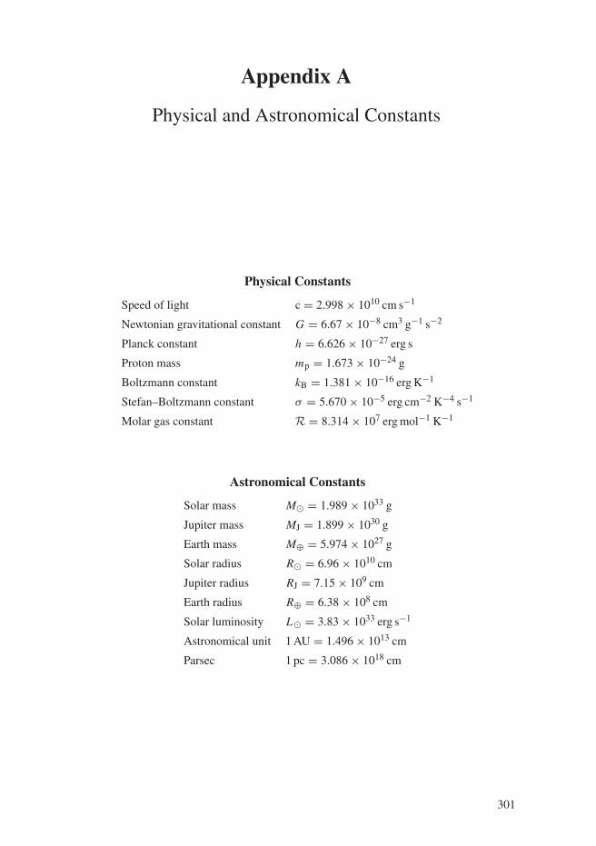
Appendix A
Physical and Astronomical Constants
Physical Constants
Speed of light c = 2.998 × 1010 cm s−1
Newtonian gravitational constant G = 6.67 × 10⁻⁸ cm3 g−1 s−2
Planck constant h = 6.626 × 10⁻²⁷ erg s
Proton mass mp = 1.673 × 10⁻²⁴ g
Boltzmann constant kB = 1.381 × 10⁻¹⁶ erg K−1
Stefan–Boltzmann constant σ = 5.670 × 10⁻⁵ erg cm−2 K−4 s−1
Molar gas constant R = 8.314 × 10⁷ erg mol−1 K−1
Astronomical Constants
Solar mass M� = 1.989 × 1033 g
Jupiter mass MJ = 1.899 × 1030 g
Earth mass M⊕ = 5.974 × 1027 g
Solar radius R� = 6.96 × 1010 cm
Jupiter radius RJ = 7.15 × 109 cm
Earth radius R⊕ = 6.38 × 108 cm
Solar luminosity L� = 3.83 × 1033 erg s−1
Astronomical unit 1 AU = 1.496 × 1013 cm
Parsec 1 pc = 3.086 × 1018 cm
301
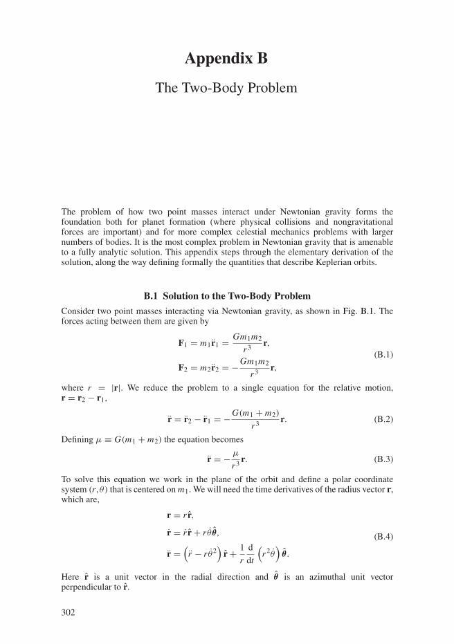
Appendix B
The Two-Body Problem
The problem of how two point masses interact under Newtonian gravity forms thefoundation both for planet formation (where physical collisions and nongravitationalforces are important) and for more complex celestial mechanics problems with largernumbers of bodies. It is the most complex problem in Newtonian gravity that is amenableto a fully analytic solution. This appendix steps through the elementary derivation of thesolution, along the way defining formally the quantities that describe Keplerian orbits.
B.1 Solution to the Two-Body Problem
Consider two point masses interacting via Newtonian gravity, as shown in Fig. B.1. Theforces acting between them are given by
F1 = m1r1 = Gm1m2
r3r,
F2 = m2r2 = −Gm1m2
r3r,
(B.1)
where r = |r|. We reduce the problem to a single equation for the relative motion,r = r2 − r1,
r = r2 − r1 = −G(m1 + m2)
r3r. (B.2)
Defining μ ≡ G(m1 + m2) the equation becomes
r = − μ
r3r. (B.3)
To solve this equation we work in the plane of the orbit and define a polar coordinatesystem (r,θ) that is centered on m1. We will need the time derivatives of the radius vector r,which are,
r = r r,
r = r r + rθ θ,
r =(r − rθ2
)r + 1
r
d
dt
(r2θ
)θ .
(B.4)
Here r is a unit vector in the radial direction and θ is an azimuthal unit vectorperpendicular to r.
302
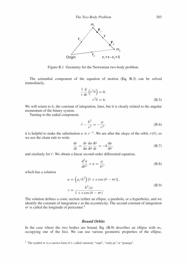
The Two-Body Problem 303
r1
r2
rF1
F2
m1
m2
Origin r1+ r – r2= 0
Figure B.1 Geometry for the Newtonian two-body problem.
The azimuthal component of the equation of motion (Eq. B.3) can be solvedimmediately,
1
r
d
dt
(r2θ
)= 0,
r2θ = h. (B.5)
We will return to h, the constant of integration, later, but it is clearly related to the angularmomentum of the binary system.
Turning to the radial component,
r − h2
r3= − μ
r2, (B.6)
it is helpful to make the substitution u ≡ r−1. We are after the shape of the orbit, r(θ), sowe use the chain rule to write
dr
dt= dr
du
du
dθ
dθ
dt= −h
du
dθ, (B.7)
and similarly for r . We obtain a linear second-order differential equation,
d2u
dθ2+ u = μ
h2, (B.8)
which has a solution
u =(μ/h2
)[1 + e cos (θ − �)] ,
r = h2/μ
1 + e cos (θ − �).
(B.9)
The solution defines a conic section (either an ellipse, a parabola, or a hyperbola), and weidentify the constant of integration e as the eccentricity. The second constant of integration� is called the longitude of pericenter.1
Bound Orbits
In the case where the two bodies are bound, Eq. (B.9) describes an ellipse with m1occupying one of the foci. We can use various geometric properties of the ellipse,
1 The symbol � is a cursive form of π , called variously “varpi”, “curly pi,” or “pomega”.

304 The Two-Body Problem
Apocenterra = a(1 + e )
m1
m2
Referencedirection(q = 0)
Pericenterrp = a(1 – e )
q
v
Trueanomalyf = q–v
r
Semi-major axis a
Semi-minoraxis b
ae
Figure B.2 Definition of quantities describing the two-body elliptical orbit of m2in a noninertial frame centered on m1.
shown in Fig. B.2, to rewrite the orbit in terms of the ellipse’s semi-major axis a andeccentricity e. The point of closest approach between the bodies is called pericenter, ata separation rp = a(1 − e) which we identify with the time when cos(θ − �) = 1.Equation (B.9) then gives
h =√
μa(1 − e2), (B.10)
and the shape of the orbit has the standard form describing an ellipse in polar coordinates,
r = a(1 − e)2
1 + e cos(θ − �). (B.11)
It can be useful to measure the progress of m2 around its orbit relative to pericenter ratherthan to an arbitrary reference direction, and so we define an angle called the true anomaly,
f ≡ θ − � . (B.12)
The other important geometric properties of the orbit are the apocenter distancera = a(1 + e) (the maximum separation between the bodies), the semi-minor axisb = a
√1 − e2, and the area within the ellipse A = πab = πa2
√1 − e2.
To compute the orbital period we note that the area swept out by m2 as it orbits m1 canbe written as
dA
dt= 1
2r2θ = 1
2h, (B.13)
which is a constant of the motion. After time t the area A = (1/2)h(t − tp), where tp isthe time of a pericenter passage. A complete orbit occurs once A = πab, at time t = P .Substituting for h gives the familiar relation for the orbital period, which does not dependon the eccentricity,
P = 2π
√a3
μ. (B.14)
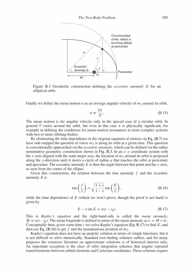
The Two-Body Problem 305
aem1
Eccentricanomaly E f
a
r
Pericenter
Circumscribedcircle, radius a,touching ellipseat pericenter
Figure B.3 Geometric construction defining the eccentric anomaly E for anelliptical orbit.
Finally we define the mean motion n as an average angular velocity of m2 around its orbit,
n ≡ 2π
P. (B.15)
The mean motion is the angular velocity only in the special case of a circular orbit. Ingeneral θ varies around the orbit, but even in this case n is physically significant, forexample in defining the conditions for mean-motion resonances in more complex systemswith two or more orbiting bodies.
By eliminating the time dependence in the original equation of motion via Eq. (B.7) wehave side-stepped the question of where m2 is along its orbit at a given time. This questionis conventionally approached via the eccentric anomaly, which can be defined via the rathernonintuitive geometric construction shown in Fig. B.3. In an x–y coordinate system withthe x-axis aligned with the semi-major axis, the location of m2 around its orbit is projectedalong the y-direction until it meets a circle of radius a that touches the orbit at pericenterand apocenter. The eccentric anomaly E is then the angle between that point and the x-axis,as seen from the center of the ellipse.
Given this construction, the relation between the true anomaly f and the eccentricanomaly E is
tan
(f
2
)=
√1 + e
1 − etan
(E
2
), (B.16)
while the time dependence of E (which we won’t prove, though the proof is not hard) isgiven by
E − e sin E = n(t − tp). (B.17)
This is Kepler’s equation and the right-hand-side is called the mean anomaly,M ≡ n(t−tp). The mean longitude is defined in terms of the mean anomaly as λ = M+� .Conceptually then, given some time t we solve Kepler’s equation (Eq. B.17) to find E, andthen use Eq. (B.16) to get f and the instantaneous position of m2.
Kepler’s equation does not have an analytic solution in terms of simple functions, but itis not difficult to solve numerically. Standard root-finding schemes suffice, and for manypurposes the extensive literature on approximate solutions is of historical interest only.An important exception is the class of orbit integration schemes that require repeatedtransformations between orbital elements and Cartesian coordinates. These schemes require
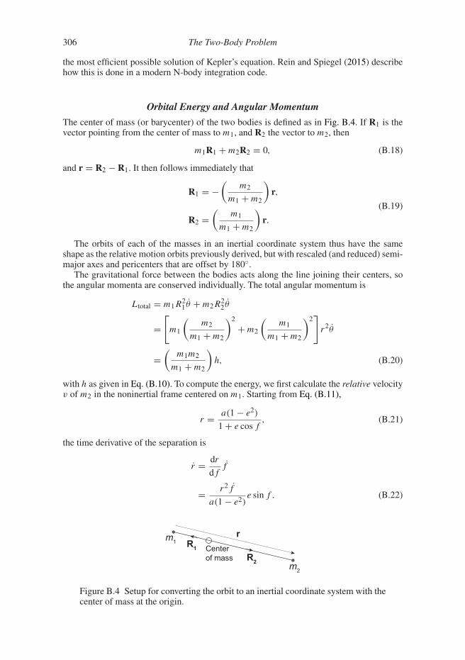
306 The Two-Body Problem
the most efficient possible solution of Kepler’s equation. Rein and Spiegel (2015) describehow this is done in a modern N-body integration code.
Orbital Energy and Angular Momentum
The center of mass (or barycenter) of the two bodies is defined as in Fig. B.4. If R1 is thevector pointing from the center of mass to m1, and R2 the vector to m2, then
m1R1 + m2R2 = 0, (B.18)
and r = R2 − R1. It then follows immediately that
R1 = −(
m2
m1 + m2
)r,
R2 =(
m1
m1 + m2
)r.
(B.19)
The orbits of each of the masses in an inertial coordinate system thus have the sameshape as the relative motion orbits previously derived, but with rescaled (and reduced) semi-major axes and pericenters that are offset by 180◦.
The gravitational force between the bodies acts along the line joining their centers, sothe angular momenta are conserved individually. The total angular momentum is
Ltotal = m1R21 θ + m2R
22 θ
=[m1
(m2
m1 + m2
)2
+ m2
(m1
m1 + m2
)2]
r2θ
=(
m1m2
m1 + m2
)h, (B.20)
with h as given in Eq. (B.10). To compute the energy, we first calculate the relative velocityv of m2 in the noninertial frame centered on m1. Starting from Eq. (B.11),
r = a(1 − e2)
1 + e cos f, (B.21)
the time derivative of the separation is
r = dr
dff
= r2f
a(1 − e2)e sin f . (B.22)
rm1
m2
R1
R2
Centerof mass
Figure B.4 Setup for converting the orbit to an inertial coordinate system with thecenter of mass at the origin.

The Two-Body Problem 307
Using the fact that f = θ we can replace r2f with h =√
μa(1 − e2). The components ofthe velocity in the radial and azimuthal direction are then
r =√
μ
a(1 − e2)e sin f, (B.23)
rf =√
μ
a(1 − e2)(1 + e cos f ) , (B.24)
and the square of the relative velocity is
v2 = r2 + (rf )2,
= μ
(2
r− 1
a
). (B.25)
Returning to the center of mass frame the total energy of the system is
Etotal = 1
2m1v
21 + 1
2m2v
22 − Gm1m2
r, (B.26)
where v1 and v2 are the velocities of the bodies in this frame. We can write v1 in termsof v via
v21 = R2
1 + R21 θ2
=(
m2
m1 + m2
)2 (r2 + r2θ2
)
=(
m2
m1 + m2
)2
v2, (B.27)
and similarly for v2. Substituting for v2 (Eq. B.25) we obtain a familiar but important result,
Etotal = −Gm1m2
2a. (B.28)
The energy of a bound elliptical orbit depends upon the semi-major axis but is independentof the eccentricity.
Inclined Orbits
In its own plane the shape of a bound orbit and the position of m2 along that orbit are fullydefined by (a,e,�,f ). Often, however, we wish to describe such an orbit in the contextof a larger system in which two or more bodies orbiting the central mass do not share acommon orbital plane. This requires thinking about two additional complications. The firstis simply how to describe an orbit with respect to an arbitrary reference plane in three-dimensional space. Two extra quantities are needed, one to measure the tilt of the orbitwith respect to the plane and one to describe the orientation of the tilt with respect toa reference direction. Conventionally, as shown in Fig. B.5, we define a reference plane(X,Y) containing a reference direction along the X axis. The inclination of the orbit iwith respect to this plane defines the tilt, with i < 90◦ corresponding to prograde orbitsand i ≥ 90◦ corresponding to retrograde orbits. The angle in the reference plane betweenthe reference direction and the point where the orbit crosses the plane in the positive Zdirection is called the longitude of the ascending node, and denoted by the symbol �. Theangle in the orbital plane between the ascending node and presenter is called the argument

308 The Two-Body Problem
X
Y
Z
xyz
^
^
^
^^^
Reference plane
Reference direction
W
w i
Ascending node
Pericenter
Focus oforbit
i - inclinationw - argument of pericenterW - longitude of ascending node
longitude of pericenterϖ = W + ω
Figure B.5 Definition of the orbital angles for a three-dimensional orbit inclinedwith respect to a reference plane.
of pericenter, and denoted by ω. The longitude of pericenter, which in the two-dimensionaldescription was just the in-plane angle between the reference direction and pericenter, ismore generally
� = � + ω. (B.29)
For an orbit that has nonzero i this is a nonobvious definition, as the longitude of theascending node and the argument of pericenter are two angles that do not lie in the sameplane. The three-dimensional orbit is then fully described by the set (a,e,�,i,�,f ).
The second complication that arises when thinking about three-dimensional orbits is themeaning of the orbital elements themselves. It is evidently most economical to describe asystem of only two bodies in its own orbital plane, so if we are thinking about inclinedorbits we are normally doing so in the context of systems of three or more bodies (or othersituations, such as orbits around an oblate star, where the simple two-body problem is onlyan approximation to the true dynamics). In a three-body system, the true orbits are notclosed ellipses/parabolae/hyperbolae, but rather something more complex which in generalcan only be determined numerically. Nonetheless, given the instantaneous positions andvelocities of any pair of bodies, together with a reference plane and reference direction, wecan go ahead and calculate orbital elements (a,e,�,i,�,f ) for that pair as if the rest ofthe system did not exist. Elements defined in this way are known as osculating elements,and represent an instantaneous two-body Keplerian approximation to the true orbit. In thecommon situation where m1 is a star and mi with i = 2,3, . . . are planets on stable orquasi-stable orbits, the planet–planet perturbations are weak and the osculating elementsdefine planetary orbits about the star that are a good approximation to the actual trajectories.One can then go further and derive equations (Lagrange’s planetary equations) for the timeevolution of the osculating elements under the action of the planet–planet perturbations,though we will not follow that line of rather technical development here.
Relativistic Precession
General relativity predicts that two-body orbits are qualitatively different from expecta-tions based on Newtonian gravity. The differences include precession of the pericenter of
The Two-Body Problem 309
elliptical orbits, precession of the longitude of the ascending node of orbits inclined withrespect to the equatorial plane of spinning masses (Lense–Thirring precession), and loss ofenergy and angular momentum due to the radiation of gravitational waves. In an orbitingsystem in which the characteristic velocity is v these effects become significant at differentorders in (v/c)2, and for planetary systems – where v c – only the lowest order effectof pericenter precession normally needs to be considered. For a binary with masses m1 andm2 and eccentricity e the longitude of pericenter of the orbit, which is fixed in space inNewtonian gravity, advances at a rate
d�
dt= 3G3/2(m1 + m2)
3/2
c2a5/2(1 − e2). (B.30)
The pericenter advances by 2π radians in a period of
PGR = 2πc2a5/2(1 − e2)
3G3/2(m1 + m2)3/2. (B.31)
For Mercury (a = 0.387 AU,e = 0.206) PGR � 3 Myr, corresponding to the “anomalous”(i.e. non-Newtonian) but measured pericenter advance of 43 arcseconds per century thatEinstein sought to reproduce as he developed general relativity. Hot Jupiters display a muchstronger effect. A low eccentricity planet at a = 0.05 AU around a solar mass star hasPGR � 1.9×10⁴ yr. Although long, these time scales can be of the same order of magnitudeas those that are associated with other secular effects, and when that secular dynamics is ofinterest relativity cannot be ignored. Examples include the long-term stability of Mercury,which is substantially altered by relativistic precession (Laskar & Gastineau, 2009), andKozai–Lidov dynamics of extrasolar planets, which is suppressed when PGR is less thanthe time scale of eccentricity oscillations (Naoz, 2016).
Relativistic dynamical effects can be incorporated into essentially Newtonian calcula-tions in a number of ways. The simplest is to add Eq. (B.30) as an explicit evolution equa-tion for the longitude of pericenter. However, it is also possible to modify the gravitationalpotential or the Hamiltonian in such a way as to reproduce the right rate of perihelionadvance, or to integrate equations of motion that include additional accelerations represent-ing post-Newtonian effects up to a specified order in (v/c)2. These approaches will notgenerally yield identical (or correct) trajectories, but are almost functionally equivalent ifthe sole focus is on secular planetary dynamics.
Parabolic and Hyperbolic Orbits
The general solution to the two-body problem (Eq. B.9) describes hyperbolic and parabolicorbits as well as elliptical ones, though the geometric meaning of a and e in these cases isdifferent. A hyperbolic orbit, with e > 1, is defined by the equation
r = a(e2 − 1)
1 + e cos(θ − �). (B.32)
Figure B.6 shows the geometry of such an orbit. In this case a is the distance, measuredalong the symmetry axis passing through the point of closest approach, between m1 and theunperturbed trajectory that m2 would have taken in the absence of gravity. More frequently,we characterize hyperbolic orbits via a combination of the impact parameter b, the distanceof closest approach rmin, and the velocity at infinity v∞. Some simple geometry gives theimpact parameter, defined as the closest approach along unperturbed trajectories, as
b = a√
e2 − 1. (B.33)

310 The Two-Body Problem
Referencedirection(q = 0)
m1
m2
Deflectionangle q
Impactparameter b
v
f
a
rmin
r
Figure B.6 Geometry of a hyperbolic orbit.
The closest approach along the actual orbit is
rmin = a(e − 1), (B.34)
occurring when f ≡ θ −� = 0. To obtain the velocity, the derivation leading to Eq. (B.25)for an elliptical orbit carries over identically apart from the definition of h, which in thehyperbolic case is
h =√
μa(e2 − 1). (B.35)
The result is that
v2 = μ
(2
r+ 1
a
), (B.36)
and the velocity as r → ∞ is v∞ = √μ/a.
Another quantity of interest is the deflection angle θ between the inbound and outboundtrajectories of m2 at large distances from m1. To compute this, we note that r → ∞ as(1 + e cos f ) → 0. The limiting values of the true anomaly at large r are thus
f∞ = cos−1(−e−1) = π ± cos−1(e−1). (B.37)
Inspection of Fig. B.6 then gives
θ = π − 2 cos−1(e−1). (B.38)
The deflection angle decreases with increasing values of e, tending to zero as e → ∞.For the special case of a parabolic orbit (e = 1) replacing a with rmin in Eq. (B.32) gives
a well-defined expression,
r = 2rmin
1 + cos(θ − �). (B.39)
A parabolic orbit has zero total energy.
Appendix C
N-Body Methods
Solving for the evolution of a system composed of N bodies interacting via their mutualgravitational force is a common problem in astrophysics. Although analytic or approximatenumerical treatments (for example those based on the Fokker–Planck equation) can be use-ful, in many cases solution of N-body problems requires the explicit numerical integrationof the trajectories traced by the bodies. A large body of technical literature (and at leastone textbook, Sverre Aarseth’s Gravitational N-Body Simulations1) is devoted to N-bodymethods, and codes that implement many of the most useful methods are readily available.This brief summary is intended to help guide aspiring N-body practitioners to the methodsand literature that may be most suitable for their problem.
Specification of the N-body Problem
The state of a system of N point masses interacting only via Newtonian gravitational forcesis fully specified once the masses mi (i = 1,N ), positions ri , and velocities vi are given atsome reference time. The evolution of the system is then described by Newton’s laws:
ri = vi, (C.1)
vi = Fi = −G
N∑j=1;j �=i
mj (ri − rj )
|ri − rj |3 , (C.2)
where the dots denote time derivatives and we have defined Fi as the force per unit mass feltby body i due to the gravitational interaction with all the remaining bodies. The problemof numerically integrating an N-body system can then be split into two parts. First, how dowe calculate the Fi? Although it is trivial to perform the explicit sum indicated in Eq. (C.2)this type of direct summation is computationally prohibitive for very large N . Approximateschemes which are much faster must then be used, but care is needed to ensure that theerrors involved do not invalidate the results. Second, given the positions and velocities atsome time t , together with an algorithm to compute the forces, how do we update the stateof the system to some later time (t+δt)? There exist an arbitrary number of finite differencerepresentations that reduce to the ordinary differential equations (ODEs) as δt → 0, and itis far from a trivial matter to decide which is best. Long-term planetary integrations poseparticular challenges since long-term error control is paramount and standard schemes thatare accurate for the integration of other ODEs can perform very poorly.
1 Unfortunately Aarseth (2003), one of the pioneers of the field, does not discuss the methods of greatest interestfor planetary integrations.
311
312 N-Body Methods
Exact and Approximate Force Evaluation
Evaluation of the force by direct summation over all pairs of particles is straightforward andyields a force calculation that is exact up to the inevitable round-off errors that result fromrepresenting real numbers with a finite number of bits. The number of force evaluations pertime step scales with the particle number as O(N2). This scaling limits the use of directsummation schemes to relatively modest particle numbers.
Exact force evaluation is necessary for the long-term evolution of a small N system ofplanets, and is preferable in all circumstances. There can, however, be situations wheretolerating some inaccuracy in the evaluation of Fi is beneficial for the overall fidelityof a calculation. If, for example, the physical number of bodies in a system exceeds themaximum number that can be integrated using direct summation, one is left with twounpalatable choices. One can either try to represent the system with a numerical proxythat has a smaller number of bodies, or integrate the true number of bodies approximately.Either choice may be appropriate depending on the problem at hand.
There are many different ways to efficiently compute an approximation to Fi . In a systemwith a large number of particles it is clear that the force felt by particle i due to its immediateneighbors will vary on a much shorter time scale than the force due to distant particles. Wecould therefore split the force into two pieces,
Fi = Fi,close + Fi,far, (C.3)
and save effort by recalculating the force from the distant particles less frequently than forthe nearby bodies. This venerable approach, known as the Ahmad–Cohen (1973) scheme,results in a modest improvement in the scaling to O(N7/4) at the expense of a smalldecrease in accuracy.
More aggressive trade-offs of accuracy for speed are not only possible but also necessaryif the system of interest has very large N (at the time of writing, in 2019, the largest planetformation calculations using direct summation have N ∼ 106). A powerful approach isto approximate the spatial distribution of the distant particles by grouping them togetherinto ever larger clumps, and evaluating the force from the center of mass of each clumprather than from the particles directly. There are many ways in which this could be done,of which the most elegant is the tree code, introduced to astrophysics by Josh Barnes andPiet Hut (1986). The basic principle is illustrated (in two dimensions) in Fig. C.1. Startingwith a cube that is large enough to enclose all of the particles within the simulation, spaceis first divided into eight sub-cubes by splitting the original cube in half along each ofthe three coordinate axes. This division of space is continued recursively until every cellcontains either one or zero particles. The lowest level cells that contain just one particleare known as the leaves on the tree. We then work backward, calculating the total massand center of mass of the cells at all higher levels of the tree, until eventually we return tothe original or root cube whose mass and center of mass are just the mass and center ofmass of the whole N-body system. When this procedure has been completed the resultingdata structure, known as an oct-tree, encodes a unique prescription for how particles canbe clumped into successively larger groups by moving up from the leaves toward the rootlevel of the tree. Unless the particle distribution is pathological, the recursive nature of thedivision scheme ensures that the depth of the tree (the number of subdivisions needed untileach cell contains at most one particle) will scale with particle number as O(log N).
With the tree in hand the force Fi on any individual particle can be calculated bytraversing the tree from the top down. At each level in the hierarchy of nested cells weevaluate the opening angles θ subtended by the cells as seen from the location of particle i.If for a particular cell
θ > θopen, (C.4)

N-Body Methods 313
Tree construction Force evaluation
Figure C.1 Illustration of how a tree structure can be imposed upon a particledistribution by recursively partitioning space into cells (squares in thistwo-dimensional quad-tree example). Once the tree has been built, the force onany given particle is determined by summing contributions from nearby particlesdirectly, while that from distant particles is evaluated approximately by groupingparticles into larger clumps and calculating the force from the center of mass ofeach clump.
then the cell in question is too close for its contents to be treated as a single object and weproceed to the next level down in the tree. If, conversely, θ < θopen then it is acceptable toevaluate the force as if the contents of the cell were a single particle located at the centerof mass of the true particle distribution within the cell.2 Using this scheme it is possible tocompute an approximate set of forces for the particles in O(N log N) time, which for largeN is a vast improvement over the N2 scaling of direct summation methods. Moreover, byvarying the cell opening criterion θopen, the accuracy of the approximation can be adjusted.
Tree codes have many advantages for large N simulations. The algorithm is very nearlycoordinate independent, works well for arbitrarily clustered mass distributions which mayhave an unusual geometry, and can be parallelized with good efficiency (Salmon, 1991;Dave et al., 1997; Springel, 2005). There is, however, a significant computational over-head inherent in the construction of the tree. As a result there are situations – particu-larly those where the particle distribution is not too strongly clustered – when it can besubstantially more efficient to compute the forces from a potential which has been pre-computed on a regular lattice of points that encloses the mass distribution. This method(Hockney & Eastwood, 1981) involves three steps:
• Starting from the locations ri and masses mi of the particles, a density field ρ(xi,yj,zk)is defined on a uniformly spaced lattice by assigning the masses of the particles to thevertices of nearby lattice cells.
• The gravitational potential in Fourier space is calculated by taking the discrete Fouriertransform of the density on the lattice, multiplied by the Green’s function for the Poissonequation. The real space potential on the lattice is then obtained by an inverse transform.
• The force at the location of each particle is found by finite differencing the potential onthe lattice.
2 It is also possible to pre-compute and store higher order multipoles of the mass distribution within cells, and touse this information to improve the accuracy of the force calculation.
314 N-Body Methods
A discrete Fourier transform can be computed efficiently using readily available and highlyoptimized libraries. As a consequence, grid methods of this kind are both fast and compar-atively easy to implement.
Softening
Two classes of problem are commonly attacked using N-body methods. In the first class,the number of bodies in the physical system – which may be planets in a planetary systemor stars in a small star cluster – is small enough that the individual particles in the N-bodysimulation can be considered to represent real bodies. Unless the bodies experience suchclose encounters that physical collisions or tidal effects become important, the only forcethat needs to be considered is Newtonian gravity with its 1/r potential, and we can aspireto integrate the orbits given this potential as accurately as possible. A common problemis that binaries may form during the simulation even if none is present initially. This willoften require the use of special methods (known as regularization) that can handle thelarge disparity in time scales between the internal motion of a single tight binary and theevolution time scale for the overall system (see e.g. Aarseth, 2003).
A second class of problems is composed of those where the number of bodies in thephysical system is far too large to represent on a one to one basis in an N-body simulation.We cannot presently hope to simulate every planetesimal in the terrestrial planet formingregion of the disk, and we will never be able to simulate galaxy formation using N-bodyparticles that have the same mass as dark matter particles. The particles in a simulationof one of these problems should not then be thought of as real bodies within the physicalsystem, but rather as tracers whose trajectories are intended to be a fair statistical sampleof the dynamics of the real system. In this regime we may need to suppress effects – suchas large-angle gravitational scattering or binary formation – that would occur unphysicallyin the N-body system due to the fact that the particle mass is much larger than the mass ofthe physical bodies. This can be done by replacing the Newtonian potential � ∝ 1/r witha softened potential, of which a simple example is
� ∝ 1
(r2 + ε2)1/2. (C.5)
The parameter ε is a user-variable softening length, which needs to be chosen so as tosuppress two-body interactions while leaving the large-scale dynamics under the action ofthe smooth potential unaffected.
Time Stepping
Once the algorithm for calculating the forces has been specified, it remains for us to decidehow to advance the system in time. This requires settling on a discrete representation of theordinary differential equations (Eq. C.2). Advancing the discrete form of the equation willintroduce errors, even if (as we assume henceforth) the forces have been computed exactlyvia direct summation. There are an infinite number of possible schemes, starting with themost naive:
rt+δti = rt
i + vtiδt, (C.6)
vt+δti = vt
i + Ftiδt . (C.7)
This scheme, known as Euler’s method, updates the position and the velocity simultane-ously using only information available at the initial time t . Euler’s method is inaccurateand should never be used. By making just a small modification, however, and computing
N-Body Methods 315
the new velocity at a time that is offset from the calculation of the new position, we arriveat the very useful leapfrog method:
rt+δt/2i = rt
i + 1
2vtiδt, (C.8)
vt+δti = vt
i + Fi (rt+δt/2i )δt, (C.9)
rt+δti = rt+δt/2
i + 1
2vt+δti δt . (C.10)
How can we compare different methods quantitatively? One way is to study how the error(the difference between the numerical solution to the discrete equations and the true solu-tion) scales as the time step is reduced. This scaling is known as the order of the method.Higher-order methods converge more rapidly toward the true solution with decreasing timestep than low-order schemes.
Long-term Planetary Integrations
The trade-offs involved in choosing an integration scheme are most difficult when theproblem involves the extremely long-term integration of planetary orbits. These aresmall-N systems, where the force integration can be completed using direct summation.Several considerations enter into the choice of time integration and numerical scheme.
• Long-term error accumulation. Evolution of a system over a billion orbits requirestypically 1010–1011 time steps. Error in the solution accumulates due to inaccuracy inthe numerical scheme, and (unavoidably) due to the use of finite-precision arithmetic.In principle, we ought to choose the most efficient scheme that keeps errors below thelevel where they affect the fidelity of the results. This is a difficult criterion to assess inpractice.
• Eccentricity. Bodies in systems where the Kozai–Lidov effect is operating, among oth-ers, can develop very high eccentricities. Some schemes that work well for near-circularorbits perform poorly as e → 1.
• Collisions and nonconservative forces. Systems in which N point particles interactsolely through Newtonian gravity have a special dynamical structure, which it can beadvantageous to preserve numerically through the use of symplectic integrators. Realsystems, however, can evolve such that physical collisions occur, and can be affected byother forces including tides and (for small particles) radiation forces. Consideration needsto be given to how to best represent these additional effects.
Chaos introduces additional considerations. Planetary systems are frequently chaotic,such that neighboring orbits diverge on a time scale that is short compared to the systemlifetime. Physically, this means that the very long-term evolution of a specific system isinherently unpredictable, as we can neither know the initial conditions to arbitrary precisionnor account for small external forces that would eventually affect the outcome. Numerically,the situation is a little different. A model N-body system (with no other forces) evolvesdeterministically from specified initial conditions, and even in the presence of chaosthat deterministic evolution can in principle be computed over any finite time interval.Doing so, however, requires the use of arbitrary precision arithmetic, whose cost iscomputationally prohibitive. Invariably the numerical solution is instead computed withfixed precision arithmetic, in which case the solution differs from the deterministic onein the presence of chaos. The numerical solution must then be interpreted in a statisticalsense, as one member of an ensemble of solutions that would result from slightly perturbedinitial conditions.

316 N-Body Methods
High-Order Methods
Integrators that advance the N-body equations using high-order numerical schemes canbe used profitably for long-term planetary integrations. IAS15, for example, is a modifiedversion of a 15th-order integrator introduced by Everhart (1985), which is implementedwithin the REBOUND code (Rein & Liu, 2012; Rein & Spiegel, 2015). This type ofintegrator can evolve systems, over long periods, without introducing numerical errors thatexceed the unavoidable lower bound imposed by the use of finite-precision arithmetic. Itis therefore a good option in situations where the accuracy of an individual calculation isof paramount importance. High-order numerical schemes can also be extended relativelyeasily to include other forces, without damage to their favorable numerical properties.
Symplectic Methods
Geometric integration schemes represent an alternative and widely used set of methodsfor planetary integrations (Kinoshita et al., 1991; Wisdom & Holman, 1991). The centralrealization behind these methods is that for long-term integrations it is desirable that thediscrete representation of the equations preserves as much as possible of the structure ofthe true equations. We know, for example, that the true dynamical system is both timereversible and energy conserving, and we might seek out integration schemes that sharesuch properties. Schemes that exactly conserve energy can be designed, but global energyconservation is a relatively weak constraint on the dynamics and this avenue is not veryprofitable. Time reversibility, on the other hand, turns out to be an extremely desirableproperty of an integration scheme, since the dissipation that leads to drift in the totalenergy is a numerical analog for a physically irreversible phenomenon. The simple leapfrogscheme is an example of a time reversible algorithm.
In addition to time reversibility, more subtle geometric properties of the true dynamicscan serve as a further guide to constructing good integration schemes. In particular, the N-body problem is an example of a dynamical system that can be described by a HamiltonianH(p,q,t) that is a function of the generalized coordinates q and generalized momenta p.The evolution of the state of a Hamiltonian system in the phase space described by thesecoordinates is given by
p = −∂H
∂q, (C.11)
q = ∂H
∂p. (C.12)
Hamilton’s equations describe how the state of the system at one time can be mapped intothe state at some later time, and we can look for properties of this map that can be carriedover to an integration scheme. Let us define the state of the system at time t to be z = (q,p).At some later time (t+δt) the state is z′ = (q′,p′). One can then show that the map betweenthese states z → z′ has the property that it is a symplectic transformation, which means thatit obeys the relation
MJMT = J. (C.13)
Here the matrices M and J are defined as
Mij = ∂z′i
∂zj
, (C.14)
J =[
0 −II 0
], (C.15)
N-Body Methods 317
with 0 and I being respectively the N × N zero and unit matrix. The important point is thatwe can apply this definition of a symplectic transformation not just to the real equationsdescribing the evolution of an N-body system (which, since the system is Hamiltonian,are guaranteed to yield symplectic maps), but also to any discrete representation of thoseequations. Demanding that the numerical scheme generate a symplectic transformation ofthe state of the system from one time step to the next enforces a very powerful constrainton the trajectories that the system can describe in phase space, and ensures that at leastqualitatively they must behave in the same way as do trajectories of the true system. For thisreason symplectic integration schemes are often preferable for very long-term integrationsof planetary dynamics, where preserving the qualitative dynamics of the system is moreimportant than obtaining the smallest error in the trajectory over the course of a few orbits.Somewhat amazingly the leapfrog scheme is not merely time reversible but also symplectic,and it is the simplest scheme that shares these two desirable traits.3
It is possible and often recommended to use symplectic methods for arbitrary N-bodyproblems. Nonetheless, the problem for which symplectic methods are best suited remainsthe small N direct integration of the Solar System or other planetary systems over very longtime scales. In this situation, it is possible to make further optimizations by noting that theSun is, by far, the dominant body in the system, and that as a result the system is almostintegrable. Formally we could write
H = HKepler + εHplanets, (C.16)
where HKepler is the Hamiltonian describing two-body motion of a planet around the Sun,and the perturbing term due to the mutual interactions between the planets is smallerby a factor that is of the order of the mass ratio between the planets and the star.To construct an integration scheme, we now approximate this Hamiltonian in the form(Wisdom & Holman, 1991; Saha & Tremaine, 1992)
H = HKepler + εHplanetsτ
∞∑n=−∞
δ(t − t0 − nτ), (C.17)
where t0 is some reference time and τ is some small fraction of an orbital period. Writtenthis way, the motion of the body is exactly Keplerian except at a set of closely spaceddiscrete intervals when the planetary perturbations are applied. The resulting integrationscheme has three steps:
• The bodies are evolved under the action of the Keplerian Hamiltonian for half a time stepτ/2. This amounts to translating the bodies along ellipses (if the orbits are bound) andcan be done analytically, either in terms of the normal Keplerian elements or in someother advantageous (non-Cartesian) coordinate system.
• The perturbing forces are evaluated in Cartesian coordinates, and each body receives animpulse that corresponds to the velocity change that would accumulate across a full timestep.
• The step is completed with another half step under the Keplerian Hamiltonian.
Although this scheme requires continual conversion between coordinate systems, theextra work that this involves is more than compensated by the fact that it is possible totake a much longer time step than would be acceptable when using an unsplit scheme.
3 We have noted that it is possible to construct symplectic integration schemes – leapfrog being an example –and that it is also possible to construct schemes that exactly preserve the total energy (though we have given noexplicit example of the latter). It may occur to the reader that it would be best of all to have a scheme that wasboth symplectic and exactly energy conserving. Alas such schemes do not exist, since it has been proved(Zhong & Marsden, 1988) that an energy conserving symplectic scheme would amount to a solution of theexact dynamical system, which is not possible if the system is nonintegrable.

318 N-Body Methods
Integrators of this class are known as mixed variable symplectic (MVS) integrators(Wisdom & Holman, 1991; Levison & Duncan, 1994; Saha & Tremaine, 1994;Chambers, 1999), and efficient implementations are available in several publicly releasedpackages. One should note that the simplest MVS schemes are not well suited to handlingclose approaches between planets (since during flybys the “perturbation” due to the planets’mutual gravity can dominate over the force from the star), and a more sophisticated versionmust be employed if the problem might involve close encounters or collisions.
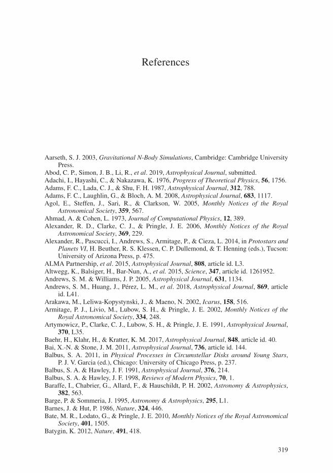
References
Aarseth, S. J. 2003, Gravitational N-Body Simulations, Cambridge: Cambridge UniversityPress.
Abod, C. P., Simon, J. B., Li, R., et al. 2019, Astrophysical Journal, submitted.Adachi, I., Hayashi, C., & Nakazawa, K. 1976, Progress of Theoretical Physics, 56, 1756.Adams, F. C., Lada, C. J., & Shu, F. H. 1987, Astrophysical Journal, 312, 788.Adams, F. C., Laughlin, G., & Bloch, A. M. 2008, Astrophysical Journal, 683, 1117.Agol, E., Steffen, J., Sari, R., & Clarkson, W. 2005, Monthly Notices of the Royal
Astronomical Society, 359, 567.Ahmad, A. & Cohen, L. 1973, Journal of Computational Physics, 12, 389.Alexander, R. D., Clarke, C. J., & Pringle, J. E. 2006, Monthly Notices of the Royal
Astronomical Society, 369, 229.Alexander, R., Pascucci, I., Andrews, S., Armitage, P., & Cieza, L. 2014, in Protostars and
Planets VI, H. Beuther, R. S. Klessen, C. P. Dullemond, & T. Henning (eds.), Tucson:University of Arizona Press, p. 475.
ALMA Partnership, et al. 2015, Astrophysical Journal, 808, article id. L3.Altwegg, K., Balsiger, H., Bar-Nun, A., et al. 2015, Science, 347, article id. 1261952.Andrews, S. M. & Williams, J. P. 2005, Astrophysical Journal, 631, 1134.Andrews, S. M., Huang, J., Perez, L. M., et al. 2018, Astrophysical Journal, 869, article
id. L41.Arakawa, M., Leliwa-Kopystynski, J., & Maeno, N. 2002, Icarus, 158, 516.Armitage, P. J., Livio, M., Lubow, S. H., & Pringle, J. E. 2002, Monthly Notices of the
Royal Astronomical Society, 334, 248.Artymowicz, P., Clarke, C. J., Lubow, S. H., & Pringle, J. E. 1991, Astrophysical Journal,
370, L35.Baehr, H., Klahr, H., & Kratter, K. M. 2017, Astrophysical Journal, 848, article id. 40.Bai, X.-N. & Stone, J. M. 2011, Astrophysical Journal, 736, article id. 144.Balbus, S. A. 2011, in Physical Processes in Circumstellar Disks around Young Stars,
P. J. V. Garcia (ed.), Chicago: University of Chicago Press, p. 237.Balbus, S. A. & Hawley, J. F. 1991, Astrophysical Journal, 376, 214.Balbus, S. A. & Hawley, J. F. 1998, Reviews of Modern Physics, 70, 1.Baraffe, I., Chabrier, G., Allard, F., & Hauschildt, P. H. 2002, Astronomy & Astrophysics,
382, 563.Barge, P. & Sommeria, J. 1995, Astronomy & Astrophysics, 295, L1.Barnes, J. & Hut, P. 1986, Nature, 324, 446.Bate, M. R., Lodato, G., & Pringle, J. E. 2010, Monthly Notices of the Royal Astronomical
Society, 401, 1505.Batygin, K. 2012, Nature, 491, 418.
319

320 References
Beckwith, S. V. W. & Sargent, A. I. 1991, Astrophysical Journal, 381, 250.Begelman, M. C., McKee, C. F., & Shields, G. A. 1983, Astrophysical Journal, 271, 70.Bell, K. R. & Lin, D. N. C. 1994, Astrophysical Journal, 427, 987.Bell, K. R., Cassen, P. M., Klahr, H. H., & Henning, Th. 1997, Astrophysical Journal,
486, 372.Benz, W. & Asphaug, E. 1999, Icarus, 142, 5.Berta-Thompson, Z. K., Irwin, J., Charbonneau, D., et al. 2015, Nature, 527, 204.Binney, J. & Tremaine, S. 1987, Galactic Dynamics, Princeton, NJ: Princeton University
Press.Birnstiel, T., Klahr, H., & Ercolano, B. 2012, Astronomy & Astrophysics, 539, id. A148.Birnstiel, T., Ormel, C. W., & Dullemond, C. P. 2011, Astronomy & Astrophysics, 525,
id. A11.Bitsch, B., Johansen, A., Lambrechts, M., & Morbidelli, A. 2015, Astronomy & Astro-
physics, 575, id. A28.Blandford, R. D. & Payne, D. G. 1982, Monthly Notices of the Royal Astronomical Society,
199, 883.Blum, J. & Wurm, G. 2008, Annual Review of Astronomy & Astrophysics, 46, 21.Borderies, N. & Goldreich, P. 1984, Celestial Mechanics, 32, 127.Boss, A. P. 1997, Science, 276, 1836.Brownlee, D., Tsou, P., Aleon, J., et al. 2006, Science, 314, 1711.Burton, M. R., Sawyer, G. M., & Granieri, D. 2013, Reviews in Mineralogy & Geochem-
istry, 75, 323.Butler, R. P., Marcy, G. W., Williams, E., et al. 1996, Publications of the Astronomical
Society of the Pacific, 108, 500.Cameron, A. G. W. 1978, The Moon and the Planets, 18, 5.Cameron, A. G. W. & Ward, W. R. 1976, Abstracts of the Lunar and Planetary Science
Conference, 7, 120.Campbell, B., Walker, G. A. H., & Yang, S. 1988, Astrophysical Journal, 331, 902.Chambers, J. 2006, Icarus, 180, 496.Chambers, J. E. 1999, Monthly Notices of the Royal Astronomical Society, 304, 793.Chambers, J. E., Wetherill, G. W., & Boss, A. P. 1996, Icarus, 119, 261.Chandrasekhar, S. 1961, Hydrodynamic and Hydromagnetic Stability, International Series
of Monographs on Physics, Oxford: Clarendon.Chatterjee, S., Ford, E. B., Matsumura, S., & Rasio, F. A. 2008, Astrophysical Journal,
686, 580.Chavanis, P. H. 2000, Astronomy & Astrophysics, 356, 1089.Chenciner, A. & Montgomery, R. 2000, Annals of Mathematics, 152, 881.Chiang, E. 2008, Astrophysical Journal, 675, 1549.Chiang, E., Lithwick, Y., Murray-Clay, R., et al. 2007, in Protostars and Planets V, B.
Reipurth, D. Jewitt, and K. Keil (eds.), Tucson: University of Arizona Press, p. 895.Chiang, E. I. & Goldreich, P. 1997, Astrophysical Journal, 490, 368.Clarke, C. J. 2009, Monthly Notices of the Royal Astronomical Society, 396, 1066.Clarke, C. J. & Pringle, J. E. 1988, Monthly Notices of the Royal Astronomical Society,
235, 635.Clarke, C. J., Gendrin, A., & Sotomayor, M. 2001, Monthly Notices of the Royal
Astronomical Society, 328, 485.Connelly, J. N., Bollard, J., & Bizzarro, M. 2017, Geochimica et Cosmochimica Acta,
201, 345.Cumming, A., Butler, R. P., Marcy, G. W., et al. 2008, Publications of the Astronomical
Society of the Pacific, 120, 531.Cuzzi, J. N., Dobrovolskis, A. R., & Champney, J. M. 1993, Icarus, 106, 102.Damjanov, I., Jayawardhana, R., Scholz, A., et al. 2007, Astrophysical Journal, 670, 1337.D’Angelo, G., Lubow, S. H., & Bate, M. R. 2006, Astrophysical Journal, 652, 1698.
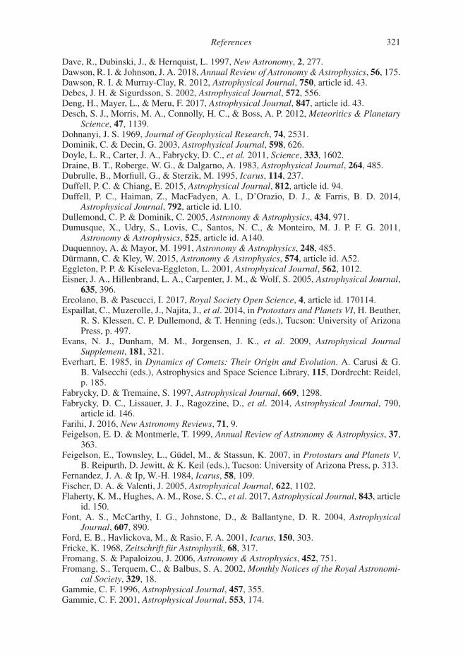
References 321
Dave, R., Dubinski, J., & Hernquist, L. 1997, New Astronomy, 2, 277.Dawson, R. I. & Johnson, J. A. 2018, Annual Review of Astronomy & Astrophysics, 56, 175.Dawson, R. I. & Murray-Clay, R. 2012, Astrophysical Journal, 750, article id. 43.Debes, J. H. & Sigurdsson, S. 2002, Astrophysical Journal, 572, 556.Deng, H., Mayer, L., & Meru, F. 2017, Astrophysical Journal, 847, article id. 43.Desch, S. J., Morris, M. A., Connolly, H. C., & Boss, A. P. 2012, Meteoritics & Planetary
Science, 47, 1139.Dohnanyi, J. S. 1969, Journal of Geophysical Research, 74, 2531.Dominik, C. & Decin, G. 2003, Astrophysical Journal, 598, 626.Doyle, L. R., Carter, J. A., Fabrycky, D. C., et al. 2011, Science, 333, 1602.Draine, B. T., Roberge, W. G., & Dalgarno, A. 1983, Astrophysical Journal, 264, 485.Dubrulle, B., Morfiull, G., & Sterzik, M. 1995, Icarus, 114, 237.Duffell, P. C. & Chiang, E. 2015, Astrophysical Journal, 812, article id. 94.Duffell, P. C., Haiman, Z., MacFadyen, A. I., D’Orazio, D. J., & Farris, B. D. 2014,
Astrophysical Journal, 792, article id. L10.Dullemond, C. P. & Dominik, C. 2005, Astronomy & Astrophysics, 434, 971.Dumusque, X., Udry, S., Lovis, C., Santos, N. C., & Monteiro, M. J. P. F. G. 2011,
Astronomy & Astrophysics, 525, article id. A140.Duquennoy, A. & Mayor, M. 1991, Astronomy & Astrophysics, 248, 485.Durmann, C. & Kley, W. 2015, Astronomy & Astrophysics, 574, article id. A52.Eggleton, P. P. & Kiseleva-Eggleton, L. 2001, Astrophysical Journal, 562, 1012.Eisner, J. A., Hillenbrand, L. A., Carpenter, J. M., & Wolf, S. 2005, Astrophysical Journal,
635, 396.Ercolano, B. & Pascucci, I. 2017, Royal Society Open Science, 4, article id. 170114.Espaillat, C., Muzerolle, J., Najita, J., et al. 2014, in Protostars and Planets VI, H. Beuther,
R. S. Klessen, C. P. Dullemond, & T. Henning (eds.), Tucson: University of ArizonaPress, p. 497.
Evans, N. J., Dunham, M. M., Jorgensen, J. K., et al. 2009, Astrophysical JournalSupplement, 181, 321.
Everhart, E. 1985, in Dynamics of Comets: Their Origin and Evolution. A. Carusi & G.B. Valsecchi (eds.), Astrophysics and Space Science Library, 115, Dordrecht: Reidel,p. 185.
Fabrycky, D. & Tremaine, S. 1997, Astrophysical Journal, 669, 1298.Fabrycky, D. C., Lissauer, J. J., Ragozzine, D., et al. 2014, Astrophysical Journal, 790,
article id. 146.Farihi, J. 2016, New Astronomy Reviews, 71, 9.Feigelson, E. D. & Montmerle, T. 1999, Annual Review of Astronomy & Astrophysics, 37,
363.Feigelson, E., Townsley, L., Gudel, M., & Stassun, K. 2007, in Protostars and Planets V,
B. Reipurth, D. Jewitt, & K. Keil (eds.), Tucson: University of Arizona Press, p. 313.Fernandez, J. A. & Ip, W.-H. 1984, Icarus, 58, 109.Fischer, D. A. & Valenti, J. 2005, Astrophysical Journal, 622, 1102.Flaherty, K. M., Hughes, A. M., Rose, S. C., et al. 2017, Astrophysical Journal, 843, article
id. 150.Font, A. S., McCarthy, I. G., Johnstone, D., & Ballantyne, D. R. 2004, Astrophysical
Journal, 607, 890.Ford, E. B., Havlickova, M., & Rasio, F. A. 2001, Icarus, 150, 303.Fricke, K. 1968, Zeitschrift fur Astrophysik, 68, 317.Fromang, S. & Papaloizou, J. 2006, Astronomy & Astrophysics, 452, 751.Fromang, S., Terquem, C., & Balbus, S. A. 2002, Monthly Notices of the Royal Astronomi-
cal Society, 329, 18.Gammie, C. F. 1996, Astrophysical Journal, 457, 355.Gammie, C. F. 2001, Astrophysical Journal, 553, 174.

322 References
Garaud, P. & Lin, D. N. C. 2004, Astrophysical Journal, 608, 1050.Garaud, P. & Lin, D. N. C. 2007, Astrophysical Journal, 654, 606.Ghosh, P. & Lamb, F. K. 1979, Astrophysical Journal, 232, 259.Gillon, M., Triaud, A. H. M. J., Demory, B.-O., et al. 2017, Nature, 542, 456.Gladman, B. 1993, Icarus, 106, 247.Godon, P. & Livio, M. 1999, Astrophysical Journal, 523, 350.Goldreich, P. & Peale, S. 1966, Astronomical Journal, 71, 425.Goldreich, P. & Sari, R. 2003, Astrophysical Journal, 585, 1024.Goldreich, P. & Schubert, G. 1967, Astrophysical Journal, 150, 571.Goldreich, P. & Tremaine, S. 1979, Astrophysical Journal, 233, 857.Goldreich, P. & Tremaine, S. 1980, Astrophysical Journal, 241, 425.Goldreich, P. & Ward, W. R. 1973, Astrophysical Journal, 183, 1051.Gomez, G. C. & Ostriker, E. C. 2005, Astrophysical Journal, 630, 1093.Gomes, R., Levison, H. F., Tsiganis, K., & Morbidelli, A. 2005, Nature, 435, 466.Goodman, A. A., Benson, P. J., Fuller, G. A., & Myers, P. C. 1993, Astrophysical Journal,
406, 528.Greenberg, R., Bottke, W. F., Carusi, A., & Valsecchi, G. B. 1991, Icarus, 94, 98.Greenberg, R., Wacker, J. F., Hartmann, W. K., & Chapman, C. R. 1978, Icarus, 35, 1.Guilet, J. & Ogilvie, G. I. 2014, Monthly Notices of the Royal Astronomical Society,
441, 852.Guillot, T., Stevenson, D. T., Hubbard, W. B., & Saumon, D. 2004, in Jupiter: The
Planet, Satellites and Magnetosphere, F. Bagenal, T. Dowling, & W. McKinnon (eds.),Cambridge: Cambridge University Press.
Gullbring, E., Hartmann, L., Briceno, C., & Calvet, N. 1998, Astrophysical Journal,492, 323.
Gundlach, B. & Blum, J. 2015, Astrophysical Journal, 798, article id. 34.Gutermuth, R. A., Myers, P. C., Megeath, S. T., et al. 2008, Astrophysical Journal, 674, 336.Guttler, C., Blum, J., Zsom, A., Ormel, C. W., & Dullemond, C. P. 2010, Astronomy &
Astrophysics, 513, article id. A56.Haisch, K. E., Lada, E. A., & Lada, C. J. 2001, Astrophysical Journal, 553, 153.Hansen, B. M. S. 2009, Astrophysical Journal, 703, 1131.Hartmann, L., Calvet, N., Gullbring, E., & D’Alessio, P. 1998, Astrophysical Journal,
495, 385.Hartmann, L., Hewett, R., & Calvet, N. 1994, Astrophysical Journal, 426, 669.Hartmann, W. K. & Davis, D. R. 1975, Icarus, 24, 504.Hartogh, P., Lis, D. C., Bockelee-Morvan, D., et al. 2011, Nature, 478, 218.Hawley, J. F., Balbus, S. A., & Winters, W. F. 1999, Astrophysical Journal, 518, 394.Hayashi, C. 1981, Progress of Theoretical Physics Supplement, 70, 35.Hernandez, J., Hartmann, L., Megeath, T., et al. 2007, Astrophysical Journal, 662, 1067.Hirayama, K. 1918, Astronomical Journal, 31, 185.Hirose, S. & Shi, J.-M. 2019, Monthly Notices of the Royal Astronomical Society, 485, 266.Hockney, R. W. & Eastwood, J. W. 1981, Computer Simulation Using Particles, New York:
McGraw-Hill.Holczer, T., Mazeh, T., Nachmani, G., et al. 2016, Astrophysical Journal Supplement Series,
225, article id. 9.Hollenbach, D., Johnstone, D., Lizano, S., & Shu, F. 1994, Astrophysical Journal, 428, 654.Holman, M. J. & Murray, N. W. 1996, Astronomical Journal, 112, 1278.Holman, M. J. & Murray, N. W. 2005, Science, 307, 1288.Holman, M., Touma, J., & Tremaine, S. 1997, Nature, 386, 254.Hornung, P., Pellat, R., & Barge, P. 1985, Icarus, 64, 295.Ida, S. 1990, Icarus, 88, 129.Ida, S. & Makino, J. 1993, Icarus, 106, 210.Ida, S., Bryden, G., Lin, D. N. C., & Tanaka, H. 2000, Astrophysical Journal, 534, 428.

References 323
Iess, L., Folkner, W. M., Durante, D., et al. 2018, Nature, 555, 220.Igea, J. & Glassgold, A. E. 1999, Astrophysical Journal, 518, 848.Ikoma, M., Nakazawa, K., & Emori, H. 2000, Astrophysical Journal, 537, 1013.Ilgner, M. & Nelson, R. P. 2006, Astronomy & Astrophysics, 445, 205.Ilgner, M. & Nelson, R. P. 2008, Astronomy & Astrophysics, 483, 815.Inaba, S., Tanaka, H., Nakazawa, K., Wetherill, G. W., & Kokubo, E. 2001, Icarus,
149, 235.Ji, H., Burin, M., Schartman, E., & Goodman, J. 2006, Nature, 444, 343.Jimenez, M. A. & Masset, F. S. 2017, Monthly Notices of the Royal Astronomical Society,
471, 4917.Johansen, A. & Lacerda, P. 2010, Monthly Notices of the Royal Astronomical Society,
404, 475.Johansen, A., Oishi, J. S., Low, M.-M. M., et al. 2007, Nature, 448, 1022.Johansen, A., Youdin, A., & Klahr, H. 2009a, Astrophysical Journal, 697, 1269.Johansen, A., Youdin, A., & Mac Low, M.-M. 2009b, Astrophysical Journal, 704, L75.Johns-Krull, C. M. 2007, Astrophysical Journal, 664, 975.Johnson, B. M. & Gammie, C. F. 2005, Astrophysical Journal, 635, 149.Johnstone, D., Hollenbach, D., & Bally, J. 1998, Astrophysical Journal, 499, 758.Joy, A. H. 1945, Astrophysical Journal, 102, 168.Jura, M. 2003, Astrophysical Journal, 584, L91.Juric, M. & Tremaine, S. 2008, Astrophysical Journal, 686, 603.Kanagawa, K. D., Muto, T., Tanaka, H., et al. 2015, Astrophysical Journal, 806, article
id. L15.Kanagawa, K. D., Tanaka, H., & Szuszkiewicz, E. 2018, Astrophysical Journal, 861, article
id. 140.Kasting, J. F., Whitmire, D. P., & Reynolds, R. T. 1993, Icarus, 101, 108.Kenyon, S. J. & Hartmann, L. 1987, Astrophysical Journal, 323, 714.Kenyon, S. J. & Luu, J. X. 1998, Astronomical Journal, 115, 2136.Kerr, M., Johnston, S., Hobbs, G., & Shannon, R. M. 2015, Astrophysical Journal, 809,
article id. L11.Kida, S. 1981, Physical Society of Japan, 50, 3517.Kinoshita, H., Yoshida, H., & Nakai, H. 1991, Celestial Mechanics and Dynamical
Astronomy, 50, 59.Kippenhahn, R. & Weigert, A. 1990, Stellar Structure and Evolution, Berlin: Springer-
Verlag.Kirkwood, D., 1867, Meteoric Astronomy: A Treatise on Shooting-stars, Fireballs, and
Aerolites, Philadelphia: J. B. Lippincott & Co.Kirsh, D. R., Duncan, M., Brasser, R., & Levison, H. F. 2009, Icarus, 199, 197.Kley, W. & Nelson, R. P. 2012, Annual Review of Astronomy & Astrophysics, 50, 211.Kokubo, E., Kominami, J., & Ida, S. 2006, Astrophysical Journal, 642, 1131.Konigl, A. 1991, Astrophysical Journal, 370, L39.Kopparapu, R. K., Ramirez, R., Kasting, J. F, et al. 2013, Astrophysical Journal, 765, 131.Korycansky, D. G. & Asphaug, E. 2006, Icarus, 181, 605.Kozai, Y. 1962, Astronomical Journal, 67, 591.Kratter, K. & Lodato, G. 2016, Annual Review of Astronomy & Astrophysics, 54, 271.Kratter, K. M., Matzner, C. D., Krumholz, M. R., & Klein, R. I. 2010, Astrophysical
Journal, 708, 1585.Krolik, J. H. & Kallman, T. R. 1983, Astrophysical Journal, 267, 610.Kuiper, G. P. 1951, Proceedings of the National Academy of Sciences, 37, 1.Kunz, M. W. 2008, Monthly Notices of the Royal Astronomical Society, 385, 1494.Kwok, S. 1975, Astrophysical Journal, 198, 583.Lada, C. J. & Lada, E. A. 2003, Annual Review of Astronomy & Astrophysics, 41, 57.Lada, C. J. & Wilking, B. A. 1984, Astrophysical Journal, 287, 610.
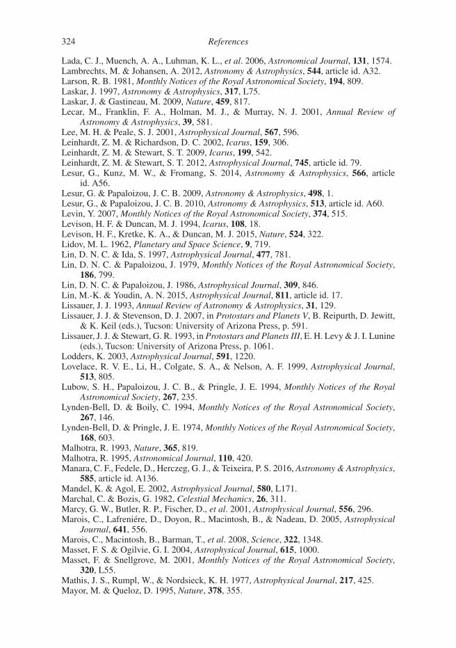
324 References
Lada, C. J., Muench, A. A., Luhman, K. L., et al. 2006, Astronomical Journal, 131, 1574.Lambrechts, M. & Johansen, A. 2012, Astronomy & Astrophysics, 544, article id. A32.Larson, R. B. 1981, Monthly Notices of the Royal Astronomical Society, 194, 809.Laskar, J. 1997, Astronomy & Astrophysics, 317, L75.Laskar, J. & Gastineau, M. 2009, Nature, 459, 817.Lecar, M., Franklin, F. A., Holman, M. J., & Murray, N. J. 2001, Annual Review of
Astronomy & Astrophysics, 39, 581.Lee, M. H. & Peale, S. J. 2001, Astrophysical Journal, 567, 596.Leinhardt, Z. M. & Richardson, D. C. 2002, Icarus, 159, 306.Leinhardt, Z. M. & Stewart, S. T. 2009, Icarus, 199, 542.Leinhardt, Z. M. & Stewart, S. T. 2012, Astrophysical Journal, 745, article id. 79.Lesur, G., Kunz, M. W., & Fromang, S. 2014, Astronomy & Astrophysics, 566, article
id. A56.Lesur, G. & Papaloizou, J. C. B. 2009, Astronomy & Astrophysics, 498, 1.Lesur, G., & Papaloizou, J. C. B. 2010, Astronomy & Astrophysics, 513, article id. A60.Levin, Y. 2007, Monthly Notices of the Royal Astronomical Society, 374, 515.Levison, H. F. & Duncan, M. J. 1994, Icarus, 108, 18.Levison, H. F., Kretke, K. A., & Duncan, M. J. 2015, Nature, 524, 322.Lidov, M. L. 1962, Planetary and Space Science, 9, 719.Lin, D. N. C. & Ida, S. 1997, Astrophysical Journal, 477, 781.Lin, D. N. C. & Papaloizou, J. 1979, Monthly Notices of the Royal Astronomical Society,
186, 799.Lin, D. N. C. & Papaloizou, J. 1986, Astrophysical Journal, 309, 846.Lin, M.-K. & Youdin, A. N. 2015, Astrophysical Journal, 811, article id. 17.Lissauer, J. J. 1993, Annual Review of Astronomy & Astrophysics, 31, 129.Lissauer, J. J. & Stevenson, D. J. 2007, in Protostars and Planets V, B. Reipurth, D. Jewitt,
& K. Keil (eds.), Tucson: University of Arizona Press, p. 591.Lissauer, J. J. & Stewart, G. R. 1993, in Protostars and Planets III, E. H. Levy & J. I. Lunine
(eds.), Tucson: University of Arizona Press, p. 1061.Lodders, K. 2003, Astrophysical Journal, 591, 1220.Lovelace, R. V. E., Li, H., Colgate, S. A., & Nelson, A. F. 1999, Astrophysical Journal,
513, 805.Lubow, S. H., Papaloizou, J. C. B., & Pringle, J. E. 1994, Monthly Notices of the Royal
Astronomical Society, 267, 235.Lynden-Bell, D. & Boily, C. 1994, Monthly Notices of the Royal Astronomical Society,
267, 146.Lynden-Bell, D. & Pringle, J. E. 1974, Monthly Notices of the Royal Astronomical Society,
168, 603.Malhotra, R. 1993, Nature, 365, 819.Malhotra, R. 1995, Astronomical Journal, 110, 420.Manara, C. F., Fedele, D., Herczeg, G. J., & Teixeira, P. S. 2016, Astronomy & Astrophysics,
585, article id. A136.Mandel, K. & Agol, E. 2002, Astrophysical Journal, 580, L171.Marchal, C. & Bozis, G. 1982, Celestial Mechanics, 26, 311.Marcy, G. W., Butler, R. P., Fischer, D., et al. 2001, Astrophysical Journal, 556, 296.Marois, C., Lafreniere, D., Doyon, R., Macintosh, B., & Nadeau, D. 2005, Astrophysical
Journal, 641, 556.Marois, C., Macintosh, B., Barman, T., et al. 2008, Science, 322, 1348.Masset, F. S. & Ogilvie, G. I. 2004, Astrophysical Journal, 615, 1000.Masset, F. & Snellgrove, M. 2001, Monthly Notices of the Royal Astronomical Society,
320, L55.Mathis, J. S., Rumpl, W., & Nordsieck, K. H. 1977, Astrophysical Journal, 217, 425.Mayor, M. & Queloz, D. 1995, Nature, 378, 355.
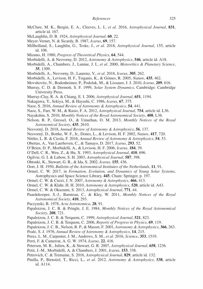
References 325
McClure, M. K., Bergin, E. A., Cleeves, L. I., et al. 2016, Astrophysical Journal, 831,article id. 167.
McLaughlin, D. B. 1924, Astrophysical Journal, 60, 22.Meyer-Vernet, N. & Sicardy, B. 1987, Icarus, 69, 157.Millholland, S., Laughlin, G., Teske, J., et al. 2018, Astrophysical Journal, 155, article
id. 106.Mizuno, H. 1980, Progress of Theoretical Physics, 64, 544.Morbidelli, A. & Nesvorny, D. 2012, Astronomy & Astrophysics, 546, article id. A18.Morbidelli, A., Chambers, J., Lunine, J. I., et al. 2000, Meteoritics & Planetary Science,
35, 1309.Morbidelli, A., Nesvorny, D., Laurenz, V., et al. 2018, Icarus, 305, 262.Morbidelli, A., Levison, H. F., Tsiganis, K., & Gomes, R. 2005, Nature, 435, 462.Movshovitz, N., Bodenheimer, P., Podolak, M., & Lissauer, J. J. 2010, Icarus, 209, 616.Murray, C. D. & Dermott, S. F. 1999, Solar System Dynamics, Cambridge: Cambridge
University Press.Murray-Clay, R. A. & Chiang, E. I. 2006, Astrophysical Journal, 651, 1194.Nakagawa, Y., Sekiya, M., & Hayashi, C. 1986, Icarus, 67, 375.Naoz, S. 2016, Annual Review of Astronomy & Astrophysics, 54, 441.Naoz, S., Farr, W. M., & Rasio, F. A. 2012, Astrophysical Journal, 754, article id. L36.Nayakshin, S. 2010, Monthly Notices of the Royal Astronomical Society, 408, L36.Nelson, R. P., Gressel, O., & Umurhan, O. M. 2013, Monthly Notices of the Royal
Astronomical Society, 435, 2610.Nesvorny, D. 2018, Annual Review of Astronomy & Astrophysics, 56, 137.Nesvorny, D., Bottke, W. F., Jr., Dones, L., & Levison, H. F. 2002, Nature, 417, 720.Nittler, L. R. & Ciesla, F. 2016, Annual Review of Astronomy & Astrophysics, 54, 53.Obertas, A., Van Laerhoven, C., & Tamayo, D. 2017, Icarus, 293, 52.O’Brien, D. P., Morbidelli, A., & Levison, H. F. 2006, Icarus, 184, 39.O’Dell, C. R., Wen, Z., & Hu, X. 1993, Astrophysical Journal, 410, 696.Ogilvie, G. I. & Lubow, S. H. 2003, Astrophysical Journal, 587, 398.Ohtsuki, K., Stewart, G. R., & Ida, S. 2002, Icarus, 155, 436.Oort, J. H. 1950, Bulletin of the Astronomical Institutes of the Netherlands, 11, 91.Ormel, C. W. 2017, in Formation, Evolution, and Dynamics of Young Solar Systems,
Astrophysics and Space Science Library, 445, Cham: Springer, p. 197.Ormel, C. W. & Cuzzi, J. N. 2007, Astronomy & Astrophysics, 466, 413.Ormel, C. W. & Klahr, H. H. 2010, Astronomy & Astrophysics, 520, article id. A43.Ormel, C. W. & Okuzumi, S. 2013, Astrophysical Journal, 771, 44.Paardekooper, S.-J., Baruteau, C., & Kley, W. 2011, Monthly Notices of the Royal
Astronomical Society, 410, 293.Paczynski, B. 1978, Acta Astronomica, 28, 91.Papaloizou, J. C. B. & Pringle, J. E. 1984, Monthly Notices of the Royal Astronomical
Society, 208, 721.Papaloizou, J. C. B. & Terquem, C. 1999, Astrophysical Journal, 521, 823.Papaloizou, J. C. B. & Terquem, C. 2006, Reports of Progress in Physics, 69, 119.Papaloizou, J. C. B., Nelson, R. P., & Masset, F. 2001, Astronomy & Astrophysics, 366, 263.Peale, S. J. 1976, Annual Review of Astronomy & Astrophysics, 14, 215.Perez, L. M., Carpenter, J. M., Andrews, S. M., et al. 2016, Science, 353, 1519.Perri, F. & Cameron, A. G. W. 1974, Icarus, 22, 416.Petersen, M. R., Julien, K., & Stewart, G. R. 2007, Astrophysical Journal, 658, 1236.Petit, J.-M., Morbidelli, A. & Chambers, J. 2001, Icarus, 153, 338.Petrovich, C. & Tremaine, S. 2016, Astrophysical Journal, 829, article id. 132.Pinilla, P., Birnstiel, T., Ricci, L., et al. 2012, Astronomy & Astrophysics, 538, article
id. A114.

326 References
Pinilla, P., Pohl, A., Stammler, S. M., & Birnstiel, T. 2017, Astrophysical Journal, 845,article id. 68.
Pollack, J. B., Hubickyj, O., Bodenheimer, P., et al. 1996, Icarus, 124, 62.Pollack, J. B., McKay, C. P., & Christofferson, B. M. 1985, Icarus, 64, 471.Pringle, J. E. 1981, Annual Review of Astronomy & Astrophysics, 19, 137.Pringle, J. E. & King, A. R. 2007, Astrophysical Flows, Cambridge: Cambridge University
Press.Pringle, J. E. & Rees, M. J. 1972, Astronomy & Astrophysics, 21, 1.Quillen, A. C. 2006, Monthly Notices of the Royal Astronomical Society, 365, 1367.Quirrenbach, A. 2006, in Extrasolar Planets. Saas-Fee Advanced Course 31, D. Queloz, S.
Udry, M. Mayor, and W. Benz (eds.), Berlin: Springer-Verlag.Ragusa, E., Dipierro, G., Lodato, G., Laibe, G., & Price, D. J. 2017, Monthly Notices of the
Royal Astronomical Society, 474, 4460.Rafikov, R. R. 2003, Astronomical Journal, 126, 2529.Rafikov, R. R. 2006, Astrophysical Journal, 648, 666.Rafikov, R. R. 2009, Astrophysical Journal, 704, 281.Rasio, F. A. & Ford, E. B. 1996, Science, 274, 954.Raymond, S. N., Barnes, R., Armitage, P. J., & Gorelick, N. 2008, Astrophysical Journal,
687, L107.Raymond, S. N., Quinn, T., & Lunine, J. I. 2006, Icarus, 183, 265.Rein, H. & Liu, S.-F. 2012, Astronomy & Astrophysics, 537, article id A128.Rein, H. & Spiegel, D. S. 2015, Monthly Notices of the Royal Astronomical Society,
446, 1424.Rein, H. & Tamayo, D. 2015, Monthly Notices of the Royal Astronomical Society, 452, 376.Ricci, L., Testi, L., Natta, A., & Brooks, K. J. 2010, Astronomy & Astrophysics, 521, article
id. A66.Rice, W. K. M. & Armitage, P. J. 2003, Astrophysical Journal, 598, L55.Rice, W. K. M., Armitage, P. J., Bate, M. R., & Bonnell, I. A. 2003, Monthly Notices of the
Royal Astronomical Society, 339, 1025.Rice, W. K. M., Armitage, P. J., Mamatsashvili, G. R., Lodato, G., & Clarke, C. J. 2011,
Monthly Notices of the Royal Astronomical Society, 418, 1356.Rice, W. K. M., Lodato, G., & Armitage, P. J. 2005, Monthly Notices of the Royal
Astronomical Society, 364, L56.Rivera, E. J., Laughlin, G., Butler, R. P., et al. 2010, Astrophysical Journal, 719, 890.Robert, C. M. T., Crida, A., Lega, E., Meheut, H., & Morbidelli, A. 2018, Astronomy &
Astrophysics, 617, article id. A98.Rogers, L. A. 2015, Astrophysical Journal, 801, article id. 41.Ros, K. & Johansen, A. 2013, Astronomy & Astrophysics, 552, article id. A137.Rossiter, R. A. 1924, Astrophysical Journal, 60, 15.Rybicki, G. B. & Lightman, A. P. 1979, Radiative Processes in Astrophysics, New York:
Wiley-Interscience.Safronov, V. S. 1969, Evolution of the Protoplanetary Cloud and Formation of the Earth
and the Planets, English translation, NASA TT F-677 (1972).Saha, P. & Tremaine, S. 1992, Astronomical Journal, 104, 1633.Saha, P. & Tremaine, S. 1994, Astronomical Journal, 108, 1962.Salmon, J. K. 1991, Parallel hierarchical N-body methods, Ph.D. thesis, California Institute
of Technology, Pasadena.Sano, T., Miyama, S. M., Umebayashi, T., & Nakano, T. 2000, Astrophysical Journal,
543, 486.Semenov, D., Henning, Th., Helling, Ch., & Sedlmayr, E. 2003, Astronomy & Astrophysics,
410, 611.Shakura, N. I. & Sunyaev, R. A. 1973, Astronomy & Astrophysics, 24, 337.Sicilia-Aguilar, A., Hartmann, L., Calvet, N., et al. 2006, Astrophysical Journal, 638, 897.
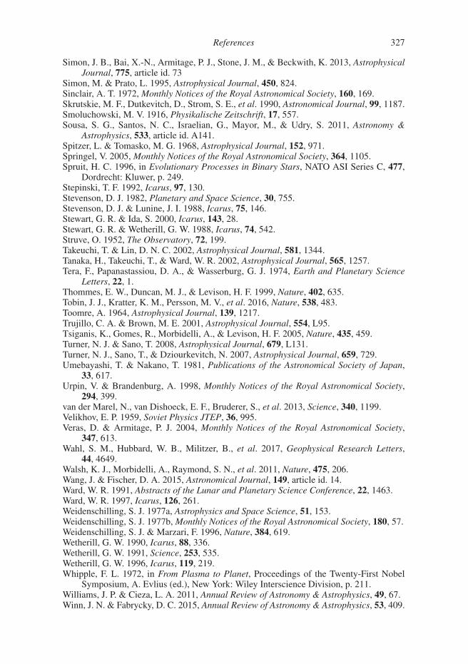
References 327
Simon, J. B., Bai, X.-N., Armitage, P. J., Stone, J. M., & Beckwith, K. 2013, AstrophysicalJournal, 775, article id. 73
Simon, M. & Prato, L. 1995, Astrophysical Journal, 450, 824.Sinclair, A. T. 1972, Monthly Notices of the Royal Astronomical Society, 160, 169.Skrutskie, M. F., Dutkevitch, D., Strom, S. E., et al. 1990, Astronomical Journal, 99, 1187.Smoluchowski, M. V. 1916, Physikalische Zeitschrift, 17, 557.Sousa, S. G., Santos, N. C., Israelian, G., Mayor, M., & Udry, S. 2011, Astronomy &
Astrophysics, 533, article id. A141.Spitzer, L. & Tomasko, M. G. 1968, Astrophysical Journal, 152, 971.Springel, V. 2005, Monthly Notices of the Royal Astronomical Society, 364, 1105.Spruit, H. C. 1996, in Evolutionary Processes in Binary Stars, NATO ASI Series C, 477,
Dordrecht: Kluwer, p. 249.Stepinski, T. F. 1992, Icarus, 97, 130.Stevenson, D. J. 1982, Planetary and Space Science, 30, 755.Stevenson, D. J. & Lunine, J. I. 1988, Icarus, 75, 146.Stewart, G. R. & Ida, S. 2000, Icarus, 143, 28.Stewart, G. R. & Wetherill, G. W. 1988, Icarus, 74, 542.Struve, O. 1952, The Observatory, 72, 199.Takeuchi, T. & Lin, D. N. C. 2002, Astrophysical Journal, 581, 1344.Tanaka, H., Takeuchi, T., & Ward, W. R. 2002, Astrophysical Journal, 565, 1257.Tera, F., Papanastassiou, D. A., & Wasserburg, G. J. 1974, Earth and Planetary Science
Letters, 22, 1.Thommes, E. W., Duncan, M. J., & Levison, H. F. 1999, Nature, 402, 635.Tobin, J. J., Kratter, K. M., Persson, M. V., et al. 2016, Nature, 538, 483.Toomre, A. 1964, Astrophysical Journal, 139, 1217.Trujillo, C. A. & Brown, M. E. 2001, Astrophysical Journal, 554, L95.Tsiganis, K., Gomes, R., Morbidelli, A., & Levison, H. F. 2005, Nature, 435, 459.Turner, N. J. & Sano, T. 2008, Astrophysical Journal, 679, L131.Turner, N. J., Sano, T., & Dziourkevitch, N. 2007, Astrophysical Journal, 659, 729.Umebayashi, T. & Nakano, T. 1981, Publications of the Astronomical Society of Japan,
33, 617.Urpin, V. & Brandenburg, A. 1998, Monthly Notices of the Royal Astronomical Society,
294, 399.van der Marel, N., van Dishoeck, E. F., Bruderer, S., et al. 2013, Science, 340, 1199.Velikhov, E. P. 1959, Soviet Physics JTEP, 36, 995.Veras, D. & Armitage, P. J. 2004, Monthly Notices of the Royal Astronomical Society,
347, 613.Wahl, S. M., Hubbard, W. B., Militzer, B., et al. 2017, Geophysical Research Letters,
44, 4649.Walsh, K. J., Morbidelli, A., Raymond, S. N., et al. 2011, Nature, 475, 206.Wang, J. & Fischer, D. A. 2015, Astronomical Journal, 149, article id. 14.Ward, W. R. 1991, Abstracts of the Lunar and Planetary Science Conference, 22, 1463.Ward, W. R. 1997, Icarus, 126, 261.Weidenschilling, S. J. 1977a, Astrophysics and Space Science, 51, 153.Weidenschilling, S. J. 1977b, Monthly Notices of the Royal Astronomical Society, 180, 57.Weidenschilling, S. J. & Marzari, F. 1996, Nature, 384, 619.Wetherill, G. W. 1990, Icarus, 88, 336.Wetherill, G. W. 1991, Science, 253, 535.Wetherill, G. W. 1996, Icarus, 119, 219.Whipple, F. L. 1972, in From Plasma to Planet, Proceedings of the Twenty-First Nobel
Symposium, A. Evlius (ed.), New York: Wiley Interscience Division, p. 211.Williams, J. P. & Cieza, L. A. 2011, Annual Review of Astronomy & Astrophysics, 49, 67.Winn, J. N. & Fabrycky, D. C. 2015, Annual Review of Astronomy & Astrophysics, 53, 409.
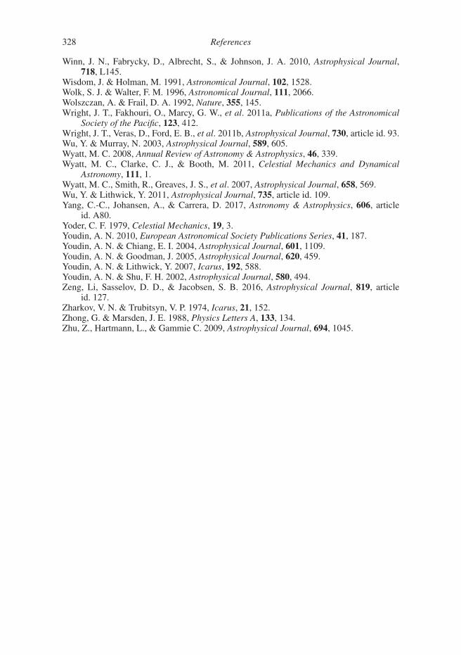
328 References
Winn, J. N., Fabrycky, D., Albrecht, S., & Johnson, J. A. 2010, Astrophysical Journal,718, L145.
Wisdom, J. & Holman, M. 1991, Astronomical Journal, 102, 1528.Wolk, S. J. & Walter, F. M. 1996, Astronomical Journal, 111, 2066.Wolszczan, A. & Frail, D. A. 1992, Nature, 355, 145.Wright, J. T., Fakhouri, O., Marcy, G. W., et al. 2011a, Publications of the Astronomical
Society of the Pacific, 123, 412.Wright, J. T., Veras, D., Ford, E. B., et al. 2011b, Astrophysical Journal, 730, article id. 93.Wu, Y. & Murray, N. 2003, Astrophysical Journal, 589, 605.Wyatt, M. C. 2008, Annual Review of Astronomy & Astrophysics, 46, 339.Wyatt, M. C., Clarke, C. J., & Booth, M. 2011, Celestial Mechanics and Dynamical
Astronomy, 111, 1.Wyatt, M. C., Smith, R., Greaves, J. S., et al. 2007, Astrophysical Journal, 658, 569.Wu, Y. & Lithwick, Y. 2011, Astrophysical Journal, 735, article id. 109.Yang, C.-C., Johansen, A., & Carrera, D. 2017, Astronomy & Astrophysics, 606, article
id. A80.Yoder, C. F. 1979, Celestial Mechanics, 19, 3.Youdin, A. N. 2010, European Astronomical Society Publications Series, 41, 187.Youdin, A. N. & Chiang, E. I. 2004, Astrophysical Journal, 601, 1109.Youdin, A. N. & Goodman, J. 2005, Astrophysical Journal, 620, 459.Youdin, A. N. & Lithwick, Y. 2007, Icarus, 192, 588.Youdin, A. N. & Shu, F. H. 2002, Astrophysical Journal, 580, 494.Zeng, Li, Sasselov, D. D., & Jacobsen, S. B. 2016, Astrophysical Journal, 819, article
id. 127.Zharkov, V. N. & Trubitsyn, V. P. 1974, Icarus, 21, 152.Zhong, G. & Marsden, J. E. 1988, Physics Letters A, 133, 134.Zhu, Z., Hartmann, L., & Gammie C. 2009, Astrophysical Journal, 694, 1045.

Index
accretion disk, see diskadiabatic temperature gradient, 228aerodynamic drag, 142–144albedo, 19Alfven velocity, 111aluminium (26Al), in Solar Nebula, 78angular momentum deficit, 275angular momentum problem (star formation),
3, 50angular momentum transport, 90, 98, 102–127asteroids, 6astrometry, 26atmosphere, condition for formation, 222azimuthal drag, 149–153azimuthal velocity (gas disk), 60, 150
Balbus–Hawley instability, 109barotropic disks, 108binary systems, Kozai resonance, 272blackbody spectrum, 20Bode’s law, 289boundary layer, 91brown dwarf, 1Brownian motion, 161
carbonate–silicate cycle, 45catastrophic disruption (threshold in collisions), 186chaos
Solar System, 270three-body problem, 285
Chiang–Goldreich model (of protoplanetarydisks), 68
chondritic meteorites, 16circulation (of resonant argument), 269co-rotation radius, 138coagulation equation, 207–210
analytic solutions, 208discrete form, 207dust growth, 163integral form, 164runaway growth, 208
collisional cascade, 293–298size distribution, 297
collisions, inelastic, 204condensation sequence, 73–74conductivity, 115continuity equation, 109convective stability, 227cooling time scale, of disk, 243core accretion, 221–237
dilute core, 239core mass, dilute, 239cosmic rays, flux, 78Coulomb logarithm, 201critical core mass, 230
analytic expressions for, 236
dead zone, 114debris disks, 293–300
collisional cascade, 293–298time evolution, 298white dwarf, 299
deuterium-burning threshold, 1diffraction limit, 20diffusion approximation, 71, 97, 226diffusion equation, 90diffusivity, 114disk
α model, 100angular momentum transport, 102debris, 87dispersal, 133evolution equation, 88flaring, 59, 63–65frequency in young clusters, 86gas temperature, 67Green’s function solution, 93ionization, 75lifetime, 87mass estimates, 54molecular line observations, 55nonlinear stability, 103photoevaporation, 134radiative equilibrium, 65ring structure, 56scale height, 58
329
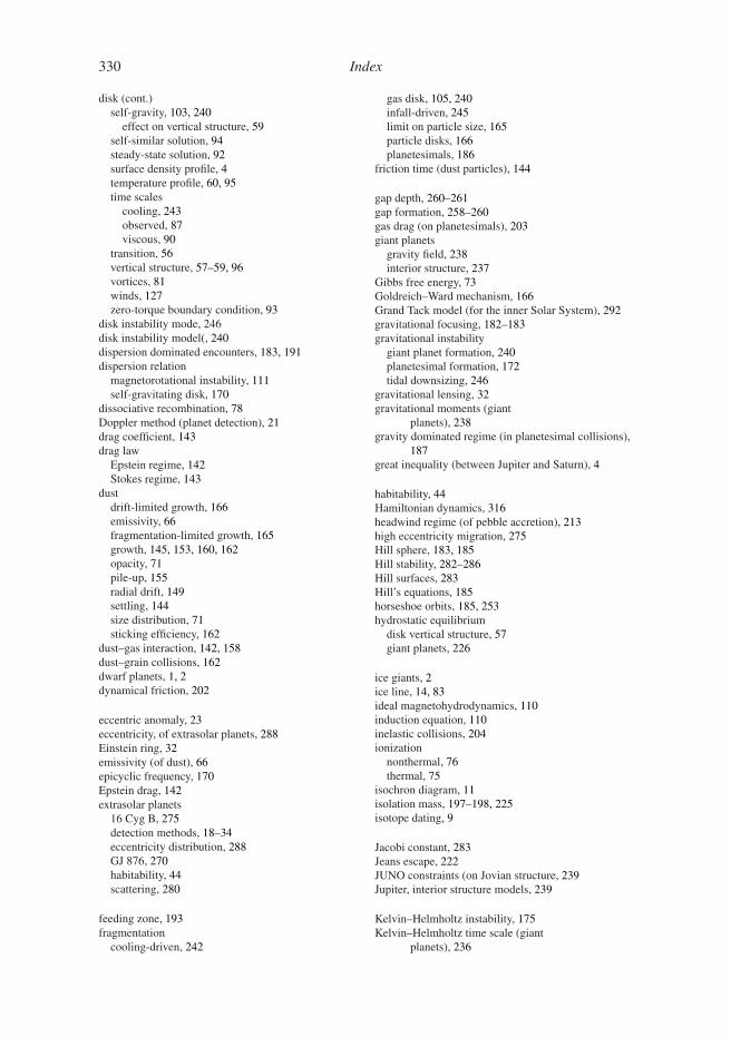
330 Index
disk (cont.)self-gravity, 103, 240
effect on vertical structure, 59self-similar solution, 94steady-state solution, 92surface density profile, 4temperature profile, 60, 95time scales
cooling, 243observed, 87viscous, 90
transition, 56vertical structure, 57–59, 96vortices, 81winds, 127zero-torque boundary condition, 93
disk instability mode, 246disk instability model(, 240dispersion dominated encounters, 183, 191dispersion relation
magnetorotational instability, 111self-gravitating disk, 170
dissociative recombination, 78Doppler method (planet detection), 21drag coefficient, 143drag law
Epstein regime, 142Stokes regime, 143
dustdrift-limited growth, 166emissivity, 66fragmentation-limited growth, 165growth, 145, 153, 160, 162opacity, 71pile-up, 155radial drift, 149settling, 144size distribution, 71sticking efficiency, 162
dust–gas interaction, 142, 158dust–grain collisions, 162dwarf planets, 1, 2dynamical friction, 202
eccentric anomaly, 23eccentricity, of extrasolar planets, 288Einstein ring, 32emissivity (of dust), 66epicyclic frequency, 170Epstein drag, 142extrasolar planets
16 Cyg B, 275detection methods, 18–34eccentricity distribution, 288GJ 876, 270habitability, 44scattering, 280
feeding zone, 193fragmentation
cooling-driven, 242
gas disk, 105, 240infall-driven, 245limit on particle size, 165particle disks, 166planetesimals, 186
friction time (dust particles), 144
gap depth, 260–261gap formation, 258–260gas drag (on planetesimals), 203giant planets
gravity field, 238interior structure, 237
Gibbs free energy, 73Goldreich–Ward mechanism, 166Grand Tack model (for the inner Solar System), 292gravitational focusing, 182–183gravitational instability
giant planet formation, 240planetesimal formation, 172tidal downsizing, 246
gravitational lensing, 32gravitational moments (giant
planets), 238gravity dominated regime (in planetesimal collisions),
187great inequality (between Jupiter and Saturn), 4
habitability, 44Hamiltonian dynamics, 316headwind regime (of pebble accretion), 213high eccentricity migration, 275Hill sphere, 183, 185Hill stability, 282–286Hill surfaces, 283Hill’s equations, 185horseshoe orbits, 185, 253hydrostatic equilibrium
disk vertical structure, 57giant planets, 226
ice giants, 2ice line, 14, 83ideal magnetohydrodynamics, 110induction equation, 110inelastic collisions, 204ionization
nonthermal, 76thermal, 75
isochron diagram, 11isolation mass, 197–198, 225isotope dating, 9
Jacobi constant, 283Jeans escape, 222JUNO constraints (on Jovian structure, 239Jupiter, interior structure models, 239
Kelvin–Helmholtz instability, 175Kelvin–Helmholtz time scale (giant
planets), 236
Index 331
Kepler’s equation, 23Keplerian orbital velocity, 21Kida vortex solution, 81kinematic viscosity, 89Kirkwood gaps, 6Kozai–Lidov dynamics, 272–275Kuiper Belt Objects (KBOs), 7
resonant capture of, 290total mass, 6
Lagrange stability, 285Late Heavy Bombardment, 292layered accretion disk model, 115–117lead–lead dating, 12leapfrog scheme, 315Ledoux criterion, 228libration (of resonant argument), 269Lindblad resonances, 252
magnetic braking, 127magnetic dynamo, 113magnetic fields
diffusivity, 114disk winds, 127instabilities, 109magnetohydrodynamics (MHD), 109non-ideal MHD, 114protostellar, 137
magnetic torque, 127magnetorotational instability, 109magnetospheric accretion, 137–140Maxwell stress, 114mean anomaly, 268mean longitude, 268mean motion, 267meteorites, 16microlensing, 32migration
eccentricity damping/growth, 264gas disk, 248–265high eccentricity tidal, 275maps, 261particles, 149planetesimal disks, 276rate, Type 2, 262simulations, 258Solar System evidence for, 290stopping mechanism, 140torque, 249torque formulae, 255Type 1, 257Type 2, 257
minimum mass Solar Nebula, 4molecular cloud cores, 49molecular viscosity, 99momentum equation, 60
N-body problem, 311leapfrog, 315softening, 314symplectic transformations, 316
Neptune, 2migration of, 290
Newtonian dynamics, 311Nice model (for the outer Solar System), 291
oligarchic growth, 206, 217opacity
analytic approximations, 72giant planet envelopes, 232Rosseland mean, 71sources within disks, 71
orderly growth, 208overlap (of resonances), 270
particle pileup, 155particle-in-box model (of planetary growth), 190–193passive disk, 60Pb–Pb dating, 12pebble accretion, 210–217
accretion rates, 216headwind (or Bondi) regime, 213headwind speed, 212lower mass limit, 214shear (or Hill) regime, 213transition mass (from headwind to shear regime),
215pendulum model (of resonance), 269photoevaporation, 134photoionization cross-section, 77Planck function, 20planet migration, see migrationplanet traps, 261planetary satellites, 9planetesimals
collisions, 186definition, 141distribution of orbital elements, 190formation of, 178formation via gravitational instability, 172–173gravitational collapse, 166growth rates, 192strength, 188velocity dispersion, 198–205
planetsdefinition, 1habitability, 44interior structure, 237pulsar, 18Solar System properties, 2
Pluto, 2capture into resonance of, 290
Poisson equation, 167protoplanetary disk, see disk
Q parameter (disk stability), 104, 167–171, 240
radial drift (of solid particles), 149radial velocity method, 21–26
biases, 23eccentric orbits, 23noise sources, 24
332 Index
radiative diffusion, 226radiative temperature gradient, 226radioactive dating, 9
lead–lead system, 12short-lived radionuclides, 13
ratio–ratio plot, 11Rayleigh criterion (spatial resolution), 20Rayleigh criterion (stability of shear flows), 103Rayleigh distribution, 190recombination, 78resonances, 3, 265–270
capture, 270–271, 290extrasolar planets, 270Kozai, 272Laplace, 9, 270libration time scale, 269Lindblad, 252mean motion, 4, 267overlap, 270, 285pendulum model, 269resonant argument, 268saturation, 264secondary, 269secular, 269, 272three-body, 269torque transfer, 251width, 269
restricted three-body problem, 282–283Reynolds number, 99
magnetic, 116Reynolds stress, 114Richardson number, 175Roche lobe, 185Rossby wave instability, 108Rosseland mean opacity, 71Rossiter–McLaughlin effect, 30rotation (T Tauri stars), 138rubble pile, 186runaway growth (of giant planets), 230runaway growth (of protoplanets), 192, 217
Saha equation, 75satellites, 9scale height, 58scattering (of giant planets), 280Schmidt number, 157Schwarzschild criterion (convective stability), 228secular chaos, 276secular dynamics, 275–276self-gravitating disk, see disk, self-gravitysettling (of dust), 144Shakura–Sunyaev α-prescription, 98–100shear dominated encounters, 183, 193shear regime (of pebble accretion), 213shot noise, 25–26silicates, 72, 73snow line, 14–16softening (in N-body problem), 314Solar Nebula, 4sound speed, 58spectral energy distribution (SED), 69–70spiral arms, 243stability (of planetary systems), 281–286
Stokes drag, 143stopping time, see friction timestreaming instability, 176strength dominated regime (in planetesimal
collisions), 187symplectic integration, 316
T Tauri stars, 77accretion rates, 52classification, 51
terrestrial planets, formation, 181–219thermal time scale (giant planet envelopes), 236three-body dynamics, 183three-body problem, 282Tisserand sphere, 185Titius–Bode law, 289Toomre Q parameter, 104, 167–171, 240torque
calculation in impulse approximation, 248formulae, 255horseshoe drag, 254Lindblad, 251linear co-rotation, 254resonant, 251thermal torque, 255
transition disks, 56transits, 27–32
secondary eclipse, 30transmission spectroscopy, 31tree codes, 312Trojan asteroids, origin of, 292true anomaly, 23turbulence
effect on particle settling, 147effect on terrestrial planet formation, 205hydrodynamic linear stability, 102hydrodynamic sources of, 102magnetic field instabilities, 109phenomenological description of, 99radial diffusion, 156self-gravitating, 102, 241
ultraviolet radiation, 134
viscosity, 90, 98, 102–114molecular, 99
viscous stirring (of planetesimals), 199vortensity, 108vortices, 81, 107
Rossby wave instability, 108
water delivery (to Earth), 15
X-ray ionization, 77
Young Stellar Objectsaccretion rates, 52classification, 51disk masses, 54
zero-velocity surfaces, 283zonal flows, 80