Planet Formation

Floris van Liere

February 6, 2009

Abstract

The formation of planets is to this day not at all well understood. Althoughwe believe to know what processes are in general responsible for formation, alot of questions are still open in the theoretical model for the formation of thetypical planetary system. This makes it an interesting and challenging fieldof research, with a lot of room for new viewpoints. In this report an overviewwill be given of what theories exist to explain the formation of planets. Alsowill be noted were these theories need to be improved, as well as what ismissing. Next, the stage after planet formation will be discussed, in whichthe planetary systems evolve due to interactions among the planets. Thenpopular and less popular methods for the detection of extrasolar planetswill be discussed, which are of vital importance for testing our knowledgeof planets. Finally we will touch upon the question of how typical our solarsystem is.

1

Contents

1 Disk formation 51.1 Stellar formation . . . . . . . . . . . . . . . . . . . . . . . . . 51.2 Disk destruction . . . . . . . . . . . . . . . . . . . . . . . . . 7

1.2.1 Photo-evaporation . . . . . . . . . . . . . . . . . . . . 7

2 Planet formation 92.1 Planet formation timescales . . . . . . . . . . . . . . . . . . . 92.2 Problems and improvements . . . . . . . . . . . . . . . . . . . 13

2.2.1 Migration due to gas drag . . . . . . . . . . . . . . . . 132.2.2 The Keplerian shear regime . . . . . . . . . . . . . . . 14

3 Planetary system evolution 15

4 Planet detection 194.1 Astrometry . . . . . . . . . . . . . . . . . . . . . . . . . . . . 194.2 Doppler spectroscopy . . . . . . . . . . . . . . . . . . . . . . . 204.3 Transits . . . . . . . . . . . . . . . . . . . . . . . . . . . . . . 204.4 Gravitational microlensing . . . . . . . . . . . . . . . . . . . . 224.5 Results obtained by planet detection . . . . . . . . . . . . . . 25

5 How typical is the solar system? 28

2

Introduction

The question of how the earth came into existence had long been a subject ofdebate for scientists and religious people alike. But the first attempt to setup a model to accurately describe planet formation scientifically, was madeby Rene Decartes in 1644, who introduced the idea that planets formed fromsystem of vortices present around the Sun. Then, later, in 1734, EmanuelSwedenborg was the one to propose the nebular hypothesis, which would bethe basis for modern thoughts on planet formation. It states that the planetsformed from a cloud of dust present around the Sun. In 1755 Immanuel Kantfurther developed this theory. However Pierre-Simon Laplace formulated asimilar theory independently around 1796, in his book Exposition of a worldsystem, and was in fact the one who first describe the process accurately.Therefore Laplace is considered by many, the founder of planetary science.Laplace had astronomy as a hobby and was intrigued by the order of thesolar system, the fact that the planets have nearly circular orbits, and thatthese orbits are in one plane, and that the orbiting directions are the same forall planets. From this he concluded that the planets and the Sun must haveformed out of one medium. This then led to the hypothesis that a largecloud (already observed in the universe at that time) contracted leadingto a faster rotation. The plane of rotation then would be the plane theplanets finally formed in, and the remaining gas ball in the center would beresponsible for forming the Sun. A modern version of this theory is still usedto this day to describe the formation of planets. The theory was howevernot free of problems and also other theories existed. In 1749 Georges-LouisLeclerc, Comte de Buffon proposed that the planets formed from a collisionbetween a comet and the Sun, from which matter was expelled condensinginto the planets. These theories however failed to describe the order in thesolar system. The nebular hypothesis was then abandoned for a long time,mostly due to the fact that it could not explained why the planets accountfor 99% of the angular momentum present in the solar system.

In the 20th century scientist began to review these theories and a lot

3

of new theories were introduced. In 1901 Thomas Chamberlin and ForestMoulton proposed the planetesimal theory in an attempt to accurately de-scribe how the protoplanetary disk condensed into the planets. Also muchwork was done on the subject by James Hopwood Jeans, Otto Schmidt,William McCrea and Micheal Woolfson. In 1978 Andrew Prentice began torevise the nebular hypothesis and then finally Victor Safronov introducedthe solar nebular disk model. This is a modern version of the initial neb-ular hypothesis and incorporates also the work done by scientists startingfrom the 20th century. In Safronov’s book Evolution of the protoplanetarycloud and formation of the Earth and the planets he published his ideas,and solved most of the problems that previous models faced.

4

Chapter 1

Disk formation

Since planets are known to orbit around stars, it is important to know howstars form in order to discuss planetary formation. In fact, planets are insome sense a by-product of stellar formation. Since the planets only makeup a fraction of the stars mass, planets will barely influence stellar evolu-tion, while stars are of vital importance to planet formation. This not onlyconcerns the central star around which the planets orbit, planet formationcan also be influenced by nearby stars shining very brightly. Although theprocess of star formation is very complicated and not yet understood toowell, a global picture of star formation will be given in this chapter. Thiswill be enough for the discussion on planet formation.

1.1 Stellar formation

Stars form from large clouds of interstellar dust. At first the density is verylow, but due to the gravitational force acting among the particles of thedust, and due to their random thermal velocities, denser regions start toappear inside the cloud. Gravitational attraction then causes the cloud tofragment into dense cores. One of these cores then further collapses, eventu-ally becoming hot enough to start shining as what is called, a class 0 object.The various stages, a star goes through in its formation are illustrated infigure 1.1. Since the innermost part of this fragment will be acceleratedmost, it will start radiating first as well. The outer part then is an envelope.The object radiates in far infrared wavelengths. By conservation of angularmomentum, the cloud will start to rotate faster and, again by the gravi-tational influence, most of the dust will settle in a rotationally supportedplane in which the cloud rotates. At this point the innermost part of the

5

cloud will start to fuse hydrogen and the actual star is born. The spectrumof this class 1 object will not look like an actual star yet because it is stillembedded in an envelope of gas and dust. This will show absorption linesin the spectrum. When the star continues to shine, the envelope will bedissipated due to stellar winds. Due to the dense disk, the class 2 objectwill still radiate in the infrared part of the spectrum. Class 3 objects consistof young stars surrounded by a transparent disk. The matter of the disk isdiscarded through various mechanisms such as photo-evaporation due to thecentral or nearby stars and accretion onto the central star. Planet formationis thought to occur during the transition from class 2 to class 3 objects.

Figure 1.1: The various stages of the formation of a stellar object are illus-trated. Taken from Klahr and Brandner [8].

6

1.2 Disk destruction

The now present disk around the young star consists of gas and dust in-herited from the interstellar medium. But since the disk is far too heavy incomparison to the final planetary system, a large part of the mass of the diskmust be lost. It is estimated that the disks mass is roughly 30% that of thecentral star, where in the solar system, the planets make up only 1% of themass of the Sun. Not only is disk mass loss a requirement for ending up withthe right mass, but it also imposes constraints on the time scales at whichplanets form. For example, if all gas in the disk is lost before protoplanetseven emerge, gas giant planets will never form because there is no gas leftfor the planets to accrete. Probably the most important mechanism for theloss of gas, especially in the outer regions of the disk, is photo-evaporation.

1.2.1 Photo-evaporation

Photo-evaporation is the process in which gas in the protoplanetary cloudis heated by radiation. This heating causes pressure gradients in the gasand results in a gas-flow in which both gas and dust can be expelled fromthe disk. To examine photo-evaporation, it is useful to consider two regimesof photon energies: extreme ultraviolet photons (EUV) with energy greaterthen 13.6 eV, and far ultraviolet photons (FUV) with energy 6 - 13.6 eV.The EUV photons can ionize hydrogen atoms, abundantly present in the gas.This heats the gas to a temperature of the order 104 K. FUV photons canbreak apart molecules, ionize carbon and heat the gas through the photo-electric effect.

Photoevaporation is especially important for O-type stars shining brightand with high flux in the EUV region. Hollenbach et al. [6] used, as theycall it, semi analytical methods to find the mass loss rate of gaseous disksaround stars. Equation (1.1) expresses the rate at which these disks areevaporated by the photons:

MEUV ≈ 4 · 10−10M¯yr−1(

φ

1041s−1

)1/2 (M?

M¯

)1/2

, (1.1)

where φ is the photon flux of the star. The 1041 photons per second repre-sents a flux that the early sun could have produced. For the most massivestars, this then corresponds to a timescale of the order 105 years to evaporatethe disk. The innermost parts of the disk will be evaporated on timescales

7

of 106 to 107 years, i.e. up to rg, the gravitational radius defined by

rg =GM?

kT≈ 100AU

(T

1000K

)−1 (M?

M¯

). (1.2)

This is far beyond the radius at which Jupiter resides. These evaporationtimes have also been observed [5]. The problem is that gas giant planetformation seems to be greatly suppressed if all gas is evaporated at shortdistances and short timescales. The problem is even more dramatic for moremassive stars. As we will see the problem can be even more severe in regionswith high star densities, were not only the central star is responsible for thegas evaporation but also external sources dissipate gas.

8

Chapter 2

Planet formation

Planets form from the accretion disk present around a young star. Rockyplanets like the terrestrial planets of the solar system form mainly from thedust inside this disk while gas giants are mainly build out of gas, with a solidcore. The formation occurs in various steps. The first step is for the dust inthe disk to start clumping together. This happens under the influence of vander Waals forces. This step is called run away accretion because the largestbodies will grow the fastest. At some point these bodies will become largeenough to gravitationally influence their environment. This is a qualitativelydifferent phase, where a small population of large bodies, called oligarches,which are inherited from the run away phase, are allowed to become roughlyequal in size. At the ice line the oligarchic growth is believed to producelarge enough bodies to form gas giant planets. At smaller radii a third stepoccurs in which the now formed protoplanets interact to form the rockyinner planets. At and beyond the ice line protoplanets can accrete gas fromthe disk if this has not already dissipated. As the third step is shown to beconsiderably shorter in duration, formation time of the terrestrial planetsand gas giant planets alike can be estimated by estimating the time it takesto form the largest protoplanets.

2.1 Planet formation timescales

To estimate formation timescales, a good starting is equation (2.1) whichexpresses the change of the mass of a protoplanet in the properties of thedisk,

9

dM

dt≈ F

Σm

2HπR2

M

(1 +

v2esc

v2m

)vm, (2.1)

where M is the mass of a forming planet, F is the ice line enhancementfactor with

F =

1 r < ril

4.2 r > ril. (2.2)

Σm is the surface density of planetesimals in the disk, H is the disk height,RM is the radius of the protoplanet, vesc is the escape velocity from thesurface of the protoplanet and vm is the relative velocity between the pro-toplanet and the planetesimals. It can be made intuitively clear that thisequation is valid. It equates the change of mass on the left hand side in theamount of mass that is available to the protoplanet. The first part expressesthe density of planetesimals in the disk, the second part is the collisionalcross section and the factor in brackets is the gravitational enhancementfactor to the cross section. Therefore the equation expresses the fact thatthe protoplanet sweeps up planetesimals available.

By making the estimations that the relative velocity vm and the diskheight H are related to the inclination im and the eccentricity em of theplanetesimal orbits,

im ≈ em/2,

vm ≈ emrΩ,

H ≈ im ≈ emr/2, (2.3)

and using vesc = (2GM/RM )1/2 and vm ¿ vesc, we can derive a scaling law:

dM

dt∝ ΣmM4/3

e2mr1/2

. (2.4)

Because for oligarchic growth the protoplanets gravitationally stir their feed-ing zone of planetesimals, em depends on M . Therefore for oligarchic growththe scaling law becomes M ∝ M2/3, while for runaway growth M ∝ M4/3.This exhibits the qualitative difference between the two regimes, because forM1 > M2, the mass ratio changes as

ddt

(M1

M2

)∝

(M1/M2)(M

1/31 −M

1/32 ) > 0 runaway

(M1/M2)(M−1/31 −M

−1/32 ) < 0 oligarchic

. (2.5)

10

So, in runaway growth, the time derivative of the mass ratio grows. There-fore the mass ratio will grow, meaning that the relatively largest mass will,will be relatively larger still, some time later. In oligarchic growth, the con-trary is true. Here the time derivative of the mass ratio is smaller then zero,so the mass ratio will shrink, implying that the difference in the massesbecomes smaller.

Next the eccentricities can be estimated in equilibrium by equating thegravitational viscous stirring timescale of the protoplanet and the randomvelocity damping due to gas drag,

em ∝ M1/3ρ−1/5gas . (2.6)

The result is

dM

dt' AΣmM2/3, (2.7)

where

A = 3.9b2/5C

2/5D G1/2M

1/6? ρ

2/5gas

ρ4/15m ρ

1/3M r1/10m2/15

,

CD is a dimensionless drag coefficient, and b determines the distance be-tween the protoplanets in the disk. Assuming that planetesimals undergono radial migration, the surface density of planetesimals Σm can be expressedas a function of the mass M of the protoplanet,

Σm(M) = Σm(0)− M

2πr∆r= Σm(0)− 31/3M

1/3? M2/3

2πbr2. (2.8)

Using this together with equation (2.7), we find

dM

dt≈ AM2/3(Σm(0)−BM2/3), (2.9)

where

B =31/3m

1/3?

2πbr2.

The result of this differential equation is

M ≈(

Σm(0)B

)3/2

tanh3

[AB1/2Σm(0)1/2

3t + tanh−1

(B1/2M(0)1/3

Σm(0)1/2

)].

(2.10)

11

The solution is a rising function which stops increasing at a certain time.This happens at a timescale

tiso =3

AB1/2Σm(0)1/2,

which is the time to reach the isolation mass

Miso =(

Σm(0)B

)3/2

.

Figure 2.1: Protoplanet sizes plotted as a function of distance to the centralstar. Plotted for 5 · 105, 106, 5 · 106 and 107 years. Plots taken from Klahrand Brandner [8]

The results are plotted in figure 4.2. The behavior is characterized by anoutward expanding front of growth. With the expression for Miso and tisowe can estimate formation times at different radii and with different diskdensities. If we take M? = M¯ and the surface density is taken to be 1, 5and 10 times that of the minimum mass model, which takes the density tobe just large enough to form all planets, we find that just beyond the iceline large planets form, with masses of the order of 1-100 M⊕ which is about

12

correct for giant planets, since giant planet cores are believed to be of order10 M⊕. Also the timescale on which this happens seems correct since after106 years there is still a significant amount of gas present to facilitate gasgiant formation. At 1 AU planets form with a mass of order 1 M⊕ whichis about correct to form terrestrial planets. However the timescale is evenshorter then that for the giant planets whereas the formation time of theearth is estimated to be order 108 years. Finally far beyond the ice line atroughly 20 AU, protoplanets fail to form even within 107 years, and whileUranus and Neptune both have significant amounts of H and He in theiratmosphere, their formation cannot be explained by this model.

2.2 Problems and improvements

We see that the theoretical model given, although it can explain giant planetformation, it does not accurately describe planet formation. Great improve-ments can be made by taking into account different effects, and althoughthis makes the calculations much more difficult, numerical methods can beused to exhibit the characteristics of these more complicated models.

2.2.1 Migration due to gas drag

One of the most logical improvements is to consider radial migration ofplanetesimals due to gas drag. This can be done by allowing the surfacedensity the change not only by planetesimal sweep up, but also by migration:

dΣm

dt=

dΣm

dt

∣∣∣∣accr

+dΣm

dt

∣∣∣∣migr

,

wheredΣm

dt

∣∣∣∣migr

= −1r

∂

∂r(rΣmrm). (2.11)

The result is a pair of coupled differential equations, which can be solvednumerically. This calculation had been performed by Thommes et al. [12]and they found that gas drag acts as a two edged sword. Firstly gas dragdamps the random thermal velocities of planetesimals in the disk, speedingup the accretion by lowering the relative velocity. But secondly gas drag alsoincreases the rate at which Σm is depleted, thereby reducing Miso. So growthis quicker but results in less heavy objects. They first did the calculationswithin the minimum mass model. The largest protoplanets that formed hada mass of less then 1 M⊕ after 10 Myears. As a result no gas giant planets

13

can form within this model at any timescale, and the Solar system wasformed from a protoplanetary disk much heavier then the minimum massmodel. With a ten times minimum mass model, they found protoplanets of∼ 10M⊕ in the region just beyond the ice line. Within the ice line earth massbodies were found, but far beyond the ice line, in what corresponds to theUranus and Neptune region, bodies of just about one tenth of an earth massformed. They also point out that to form sufficiently large protoplanetsat these radii, at least 80 times the minimum mass model is required tofacilitate large enough bodies within 10 Myrs, far beyond the typical range ofobservationally inferred disk masses. Nevertheless this model does properlyexplain the formation of giant planets.

2.2.2 The Keplerian shear regime

Another effect caused by gas in the protoplanetary disk is that it has theeffect of slowing down planetesimals orbiting in the disk. If this slowingdown is big enough accretion can happen in the shear dominated regime, inwhich the planetesimals follow closely the orbit of the gas. This is opposedto the dispersion dominated regime as discussed previously, where planetes-imal motion is due to random thermal motion and scattering. Because inthe former regime the relative velocity is small the accretion rate is greatlyenhanced. Because the planetesimals follow the gas so closely, their incli-nation will be relatively small. In the most extreme case this leads to thefact that the disk height is roughly equal to the protoplanet cross sectionresulting in a very efficient accretion of planetesimals. The accretion ratethen can be seen as a 2-dimensional process. Although only a small partof planetesimals is likely to be in the shear dominated regime, Rafikov [10]showed that only 1% of the total mass needs to be in this region for theprotoplanet mass change to be described by this regime.

14

Chapter 3

Planetary system evolution

Now that we know how a planetary system evolves from a cloud of dust andgas towards a star with a number of planets orbiting around it in nearlycircular orbits, it is a good question to ask whether these systems are stableor not. From observations it is known that a large proportion of planetshave large eccentricities. These eccentricities can not be properly explainedusing the formation model given in the last chapters. Therefore it is naturalto assume that after this first phase of formation a second phase exists inwhich the planets interact among each other. These interactions are of thegravitational kind when the orbits of the planets happen to be close enough.Since the theoretical models are not yet elaborate enough to predict whatthe relative distances of the planets are after the formation stage, it is usefulto look at a model in which the planets inherited from the formation phaseare present in a disk in circular orbits, with random spacings between them.A way of dealing with this stage, is by simply assuming that planets havealready formed, and starting from a system of nearly circular orbiting plan-ets, and see how this system evolves. Juric and Tremaine did simulations fursuch systems [7]. They started with systems of three, ten and fifty planets,and considered only gravitational force between the planets. Collisions werefully elastic so that planets could merge with each other or with the centralstar, without fragmentation. In figure 3.1 the average number of planetsis plotted as a function of time. As can be seen, the systems are highlyunstable, since after 106 years most systems consist of only a few planets.Also the final number of planets seems to be insensitive to the initial num-ber. It is important to note that similar values were obtained by Adams andLaughlin [3] and Papaloizou and Terquem [9], despite the fact that they useddifferent initial conditions. The actual number of planets is estimated to be

15

too low, because tidal forces by the central star are neglected. Tidal forcesact as to circularize orbits of planets. Therefore, at closer orbits, less planetswill collide or be expelled. Then they also plotted the distribution functionthey found as a function of the eccentricities of the planets, averaged overthe systems for the various system sizes (figure 3.2). The planetary systemsare highly eccentric, with almost no circular orbits.

To compare, in figure 4.5 observed eccentricities are plotted. Althoughthese planets are subject to strong selection effects, this should not influ-ence the picture since the simulations point out that eccentricity scales withneither mass nor distance. As can be seen, most planets have an eccen-tricity smaller then 0.2. From the simulations it is clear though that mostplanets should have an eccentricity of 0.2 ≤ e ≤ 0.4. Juric and Tremainegive two explanations for this [7]. Firstly, the observed planets are found insystems of various lifetimes, suggesting that a part of these systems has notyet had time to develop instabilities. This will show an excess in circularor nearly circular orbits. Secondly, as pointed out before, the planets in thesimulations at smaller orbits are not subject to tidal forces present in realplanetary systems. This will also account for a larger proportion of planetswith small eccentricities in the observations.

16

Figure 3.1: Average number of planets as function of time. Figure takenfrom Juric and Tremaine [7].

17

Figure 3.2: Cumulative distribution functions of planet eccentricities. Figuretaken from Juric and Tremaine [7].

18

Chapter 4

Planet detection

This chapter will treat some techniques to detect extrasolar planets. This isobviously of great importance to the study of planets since models shouldbe verified by what is observed. Although today’s measurement are some-what biassed due to technical limitations, there is still a lot to be concludedfrom them, and combining several different detection techniques may revealdifferent properties.

4.1 Astrometry

Astrometry is an indirect detection technique that was the first one to beapplied in the search for planets. If a planet orbits a star, planet and star willactually be orbiting a common center point, called the barycenter. Since thestars mass is much bigger then the planets mass, the distance of the planet tothe barycenter will be much bigger then the stars distance, but neverthelessnon-zero, and if it is big enough, the star can be directly observed in motionaround it. Although only the velocity of the star is known, the distance of theplanet to the star can be calculated as well as the mass of the planet. This issimple mechanics and can be done by using Kepler’s third law P 2/r3 = cst.,and the law of gravitation GmM?

r2 = mv2

r , resulting in:

r = 3

√GM?

4π2P 2, (4.1)

and

m =M?v?

v=

√M?r

Gv? (4.2)

.

19

Depending on the planet orbiting the star, astrometry can take quitea long time to detect a planet, since the period of the star around thebarycenter is the same as the planets period, and considering the fact thatastrometry is more likely to find planets with large orbits, the period caneasily be ten years or more. This fact together with the fact that the starsdisplacement is hard to spot, makes astrometry a little used technique forthe detection of planets.

4.2 Doppler spectroscopy

Doppler spectroscopy or radial velocity measurement is a detection tech-nique that detects the same motion of a star as is measured with astrometrybut does this by looking at a doppler shift of the stellar light, as the star ismoving towards the earth and away from it. One disadvantage as comparedto astrometry is that the line of sight must make an angle with the planetaryplane in order the detect the doppler shift. However, since it is far easier tospot the doppler shift then it is to spot the displacement directly, dopplerspectroscopy is far more appealing then astrometry is. As an example, withastrometry, differences in the speed of a star can be measured down to 10m/s, where with doppler spectroscopy differences of 1 m/s can be measured.

As already explained, the planetary disk has to be in the line of sightin order to be able to detect a planet at all, however is the planetary diskmakes an angle with the line of sight, there will only be a partial effect,resulting in an underestimation of the planets mass. Other techniques arethen used to determine the tilt of the plane. Since the velocity of the staris measured, as with astrometry, the distance of the planet to star and themass of the planet can be calculated both.

4.3 Transits

Another useful method for planet detection is the method of transits. Withthis method, a planet is spotted when it passes in front of its parent star,taking away a fraction of the stellar light. The reduction of light emittedthen depends on the radii of planet and star.

One obvious disadvantage, is the fact that the sphere of the planet’sorbit radius is very large compared to the stellar disk, making the chancethat a planet passes in front of a star very small. However, planets with asmaller orbit are easier to detect, making this method suitable for findingearth like planets.

20

To calculate the probability that a given planetary disk had the rightinclination for a transit to be observable, consider figure 4.1, where i is the

Figure 4.1: Calculating the transit probability. Taken from Sackett [11].

inclination with respect to the plane in the line of sight and d(t) is theprojected distance of the planet to the star. Now a transit can only beobserved when r cos i ≤ R? + Rp, with R? the radius of the star and Rp

the radius of the planet. Now cos i takes values between 0 and 1, and sinceit is equally likely to take any value in between for a random orbit we cancalculate the desired probability by

Ptransit =∫ (R?+Rp)/r0 d cos i∫ 1

0 d cos i=

R? + Rp

r. (4.3)

In all but the most extreme cases, we have R? À Rp so that equation 4.3can be written as Ptransit = R?/r. For a planet at 1 AU this means that thetransit probability is 4.6 · 10−3, so that for measurements on which reliablestatistics can be done thousands of stars have to be scanned. Therefore thismethod will not tell wether there is a planet around one particular star.

Another disadvantage is that the method is subject to a high rate of falsedetections. The light emitted by stars is constantly fluctuating a tiny bit,therefore it is hard to distinguish a fluctuation and a small orbiting planet.

21

This can however be overcome partly by doing measurements over very longperiods of time.

Why then are transits useful? Were the velocity measurements discussedin the previous sections determine the mass and the distance to the star ofthe target planet, the transit method provides information about the size ofthe planet. If the stellar size is known, the size of the planet can be deducedby looking at the amount of light hidden by the planet. Furthermore bycombining the transit method with spectroscopy, information about the at-mosphere of the planet is won. Stellar light passing through the atmospherewill show absorption lines of the components in the atmosphere. This thenis a good indication of whether conditions on the planet could resembleconditions on earth.

Currently there is a number of projects using the transit method to detectplanets. The Spitzer space telescope is used for this. In 2006 the COnvec-tion ROtation and planetary Transits (COROT) program was launched. Todate COROT has detected 7 exoplanets. The most recent discovery, wasannounced on 3 February 2009, very recent at the time of writing, and isthe smallest exoplanet detected to this date, with a radius less then twicethe earth radius [1]. Although the precise environment is unknown at thetime, it is known that this planet is a rocky planet, just like the terrestrialplanets.

Another program which is currently still under development is the Keplermission. Kepler’s main goal is to spot transits.

4.4 Gravitational microlensing

Planets can also be detected by gravitational microlensing. This happenswhen a star (in the case of planet detection) moves close to the line of sightof an observer to a background star. The light rays of the background sourceget bended by the gravitational lens, such that multiple images of the sourcewill be observed (see figure 4.2). From general relativity we know that thedeflection angle α can be expressed in terms of the Schwarzschild radiusRS of the lens and r, the closest point of approach of the light rays to thesource, if r À RS ,

α =4GM

c2r=

2RS

r. (4.4)

Using this and some geometry considerations

θSDS = rDS

DL− (DS −DL)α. (4.5)

22

Figure 4.2: Left picture: The light rays of a background source S areshown, as they are bended by a lens L. Images I1 and I2 will be observed.α is the angle between the two images. Right picture: The imagesare shown as seen by an observer. The circle at an angle θs gets distortedinto two flattened and bended circles. θE is the Einstein radius, is thecharacteristic distance. Figure taken from Sackett [11].

which can be written asθS = θ − DSL

DSα, (4.6)

which is known as the lens equation. It equates the angular position ofthe images θ, to the position of the source and the deflection angle. Usingr = DLθ and

θE =

√2RSDLS

DSDL. (4.7)

This can be written asθ2 − θSθ − θ2

E = 0. (4.8)

This equation then yields two solutions: the angular positions of the twoimages.

To calculate the magnification of the images, it is important to note thatthe brightness of each image is unchanged. This means that only the ratioin area is important to the magnification: the magnification is just the ratioof image area to source area. It can be shown that the magnification thencan be written as

A =u2 + 2

u√

u2 + 4, (4.9)

with u = θs/θE .

23

Figure 4.3: An additional peak in the lightcurve is seen due to lensing byan exoplanet. The time is in days. Figure taken from Sackett [11].

What is interesting in the case of planet detection, is microlensing bybinary systems. Since there are now two gravitational sources, the imagepatterns will be more complicated. For the case of single lens, there arefour parameters: the time tE it takes to cross the Einstein-ring, the impactparameter umin, the time of maximum amplification t0 and the flux of thesource F0. In the cases of a binary system there are however three additionalparameters needed to describe lensing: the separation b of the lenses, theratio of their masses q and the angle φ of the source trajectory with thebinary axis. Although there are much free parameters it is actually possibleto predict the images in real time. The lightcurve of a detected planet isshown in figure 4.3. Since the lightcurve can be predicted real time, themass of the planet and the distance to the star can be measured usingmicrolensing.

A huge disadvantage is that lensing experiments cannot be repeated. Thechance that a star crosses a background source is small, and the star will notreturn to the same spot. On the other hand, it is true that microlensing canbe used on far larger distances then any other detection method, however thiscan also be seen as a disadvantage, because planets found by microlensingare not liable to examining any further.

Since it is hard to predict when a star will pass a background star, usuallylarge robotic networks of telescopes are used to scan the sky for lensing

24

events. The Optical Gravitational Lensing Experiment (OGLE) is a Polishprogram designed to detect dark matter using microlensing. Aside from thatthey also found a number of exoplanets. Then there is the Probing LensingAnomalies NETwork (PLANET), that has several telescopes around theworld onn the southern hemisphere. PLANET is even able to detect earthmass planets.

4.5 Results obtained by planet detection

The first confirmed discovery of an exoplanet was made in 1988 by B. Cam-bell et al [4]. It was very difficult to verify at the time due to technicallimitations. At first the number grew slowly but now that telescopes haveimproved significantly, exoplanets are more readily detected. To this date339 exoplanets have been detected [2]. Most of these planets are detectedaround different stars, although also multiplanet systems are known. Thereason is a bias, smaller, for now undetectable, planets are likely to bepresent in these systems.

Figure 4.4: Mass distribution for 101 observed planets. The data is obtainedby the Lick, Keck, and AAT Doppler survey. A powerlaw is fitted to thedata. Picture taken from Klahr and Brandner [8].

In figure 4.4 a distribution is plotted for observed planetary masses asobtained by a doppler survey of 1330 target stars. A powerlaw is fitted tothe data. In figure 4.5 an eccentricity distribution is plotted for the same

25

Figure 4.5: Eccentricity distribution for 101 observed planets. The data isobtained by the Lick, Keck, and AAT Doppler survey. Taken from Klahrand Brandner [8].

planets. As can be seen, the planets are highly eccentric, especially forlarger orbits. For smaller orbits, the eccentricities are smaller, probablydue to tidal circularization of the central star. These eccentricities are notexplained by the theoretical models of planet formation, however they canbe explained by assuming that the planetary systems are unstable, so thatthese eccentricities occur only after the planets have already formed. Thisis also explained in chapter 3. A property was also exhibited by plotting themetallicity of stars versus the occurrence of planets. As clearly seen fromfigure 4.6, there is a strong correlation between the amount of iron presentin the star, and the number of planets. The physical reason for this iscalled nature of nurture, and is the effect that systems with high metallicityare subject to increased small particle condensates. The iron acts as thedust in the protoplanetary cloud. Hence there is an increased formation ofplanetesimals and therefore also an increased formation of planets. This isstrong support for the accretion model of planet formation.

26

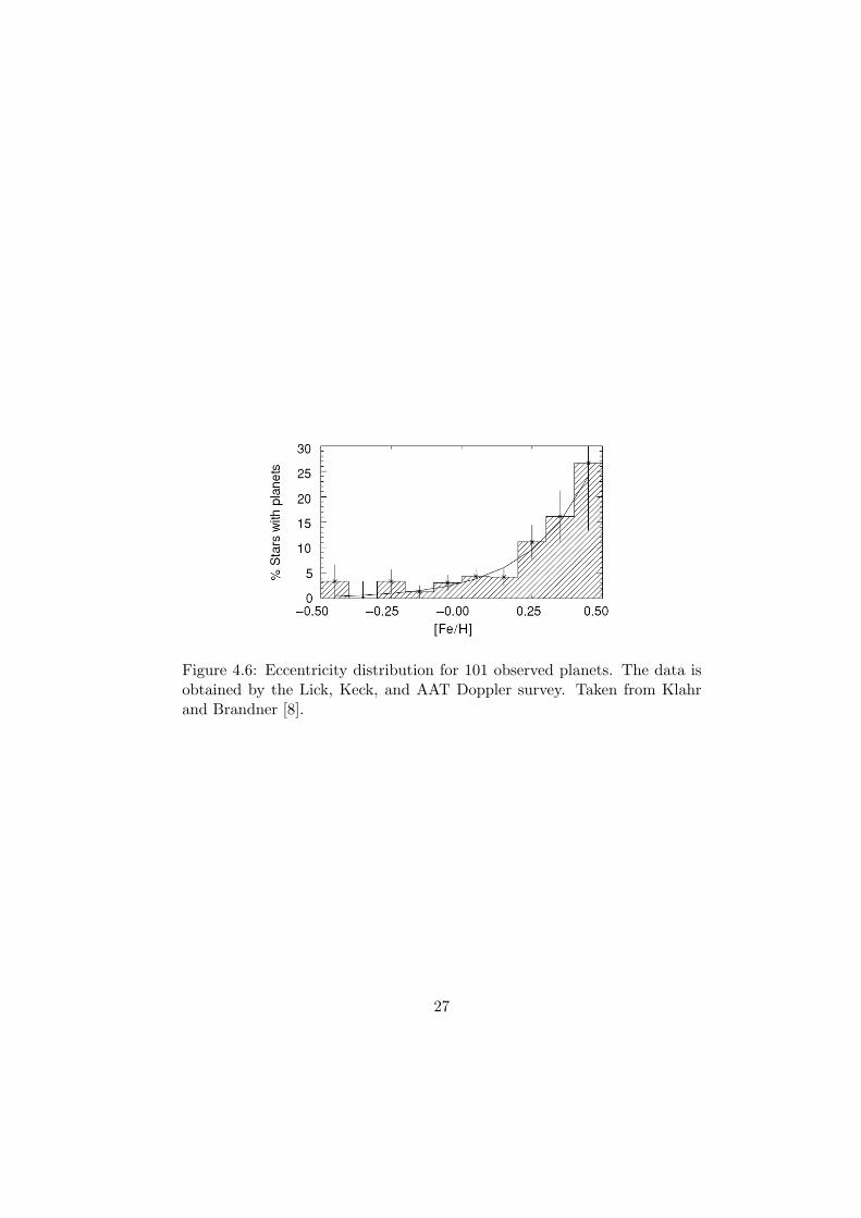
Figure 4.6: Eccentricity distribution for 101 observed planets. The data isobtained by the Lick, Keck, and AAT Doppler survey. Taken from Klahrand Brandner [8].

27

Chapter 5

How typical is the solarsystem?

As a final part of this report, it is nice to discuss the question: How typical isthe solar system?. To start with the most striking difference with observeddata, extra solar planets are seen to be highly eccentric. The most likelyexplanation for this is that the solar system is simply not old enough forthe planets within it, to have interacted and obtained more eccentric orbits.However, the age of the solar system is thought to be of the order 109 yearswhereas simulations show that instabilities in planetary systems take in theorder 106 years to develop. The most logical explanation is that the solarsystem is unusually stable compared to other planetary systems. It mustbe noted though, that these simulations are not yet that sophisticated andleave much room for improvement, most notably in the initial conditions.According to theory however the solar system is typical for young stellarsystems, but then again these theories were formed to fit the solar model,so not much can be said on that account.

Of the 339 detected planets only 36 systems are known to contain mul-tiple planets. This is mostly due to technical limitations though. A lotof exoplanets are however hot jupiters. When a hot jupiter is present, itis unlikely that any terrestrial planets are present in that system, becausethese planets close to their host star, push any other planet inwards, by mi-gration, leaving little or no room for smaller planets at close orbits. Thesesystems then are quite unlike the solar system. It is not known what per-centage of planets is a hot jupiter. This is hard to estimate due to biassesin measurements, and limited sample size.

Although it will be possible in the future to determine exoplanets atmo-

28

spheres by examining transits, to this day no such measurements have beendone. There are some promising projects for this, and in the future morewill be known about possible earth-like conditions on exoplanets.

The bottom line is that it is to preliminary to draw any conclusionsfrom measurements and theories alike. Great developments have taken placethough and in the near future much more will be known on the subject.

29

Bibliography

[1] February 5, 2009. http://www.esa.int/esaCP/SEM7G6XPXPF index 0.html.

[2] February 5, 2009. http://exoplanet.eu/catalog.php.

[3] F. C. Adams and G. Laughlin. Migration and dynamical relaxation incrowded systems of giant planets. Icarus, 163(2):290–306, 2003.

[4] B. Campbell, G. A. H. Walker, and S. Yang. A search for substellarcompanions to solar-type stars. The Astrophysical Journal, 331(1):902–921, 1988.

[5] W. J. Henney and C. R. O’Dell. A keck high-resolution spectro-scopic study of the orion nebula propllyds. The Astronomical Journal,118(5):2350–2368, 1999.

[6] D. Hollenbach, D. Johnstone, S. Lizano, and F. Shu. Photoevaporationof disks around massive stars and application to ultracompact H IIregions. The Astrophysical Journal, 428(2):654–669, 1994.

[7] M. Juric and S. Tremaine. Dynamical origin of extrasolar panet eccen-tricity distribution. The Astrophysical Journal, 686(1):603–620, 2008.arXiv:astro-ph/0703160v2.

[8] H. Klahr and W. Brandner. Planet Formation, Theory, Observations,and Experiments. Cambridge University Press, 2006.

[9] J. C. B. Papaloizou and C. Terquem. Dynamical relaxation and massiveextrasolar planets. MNRAS, 325(1):221–230, 2001.

[10] R. R. Rafikov. Fast accretion of small planetesimals by protoplanetarycores. The Astronomical Journal, 128:1348–1363, 2004.

30

[11] P. D. Sackett. Searching for unseen planets via occultation and mi-crolensing. Kluwer Academic Publishers, page 189, 1999. arXiv:astro-ph/9811269v1.

[12] E. W. Thommes, M. J. Duncan, and H. F. Levison. Oligarchic growthof giant planets. Icarus, 161(2):431–455, February 2003. arXiv:astro-ph/0303269v1.

31