A&A 540, A88 (2012)DOI: 10.1051/0004-6361/201118678c© ESO 2012

Astronomy&

Astrophysics

Quasi full-disk maps of solar horizontal velocitiesusing SDO/HMI data

Th. Roudier1,2, M. Rieutord1,2, J. M. Malherbe3, N. Renon4, T. Berger5, Z. Frank5, V. Prat1,2,L. Gizon6,7, and M. Švanda6,8,9

1 Université de Toulouse, UPS-OMP, IRAP, Toulouse, Francee-mail: thierry.roudier@irap.omp.eu

2 CNRS, IRAP, 14 avenue Edouard Belin, 31400 Toulouse, France3 LESIA, Observatoire de Paris, Section de Meudon, 92195 Meudon, France4 CALMIP, DTSI Université Paul Sabatier, Université de Toulouse 31062 Toulouse, France5 Lockheed Martin Advance Technology Center, Palo Alto, CA, USA6 Max-Planck-Institut für Sonnensystemforschung, Max-Planck-Strasse 2, 37191 Katlenburg-Lindau, Germany7 Institut für Astrophysik, Georg-August Universität Göttingen, 37077 Göttingen, Germany8 Astronomical Institute, Academy of Sciences of the Czech Republic (v. v. i.), Fricova 298, 25165 Ondrejov, Czech Republic9 Astronomical Institute, Faculty of Mathematics and Physics, Charles University in Prague, V Holešovickách 2, 18000 Prague 8,

Czech Republic

Received 19 December 2011 / Accepted 18 February 2012

ABSTRACT

Aims. For the first time, the motion of granules (solar plasma on the surface on scales larger than 2.5 Mm) has been followed over theentire visible surface of the Sun, using SDO/HMI white-light data.Methods. Horizontal velocity fields are derived from image correlation tracking using a new version of the coherent structure trackingalgorithm. The spatial and temporal resolutions of the horizontal velocity map are 2.5 Mm and 30 min, respectively.Results. From this reconstruction, using the multi-resolution analysis, one can obtain to the velocity field at different scales withits derivatives such as the horizontal divergence or the vertical component of the vorticity. The intrinsic error on the velocity is∼0.25 km s−1 for a time sequence of 30 min and a mesh size of 2.5 Mm. This is acceptable compared to the granule velocities, whichrange between 0.3 km s−1 and 1.8 km s−1. A high correlation between velocities computed from Hinode and SDO/HMI has been found(85%). From the data we derive the power spectrum of the supergranulation horizontal velocity field, the solar differential rotation,and the meridional velocity.

Key words. Sun: granulation – Sun: rotation – Sun: general

1. Introduction

The Sun is a star whose plasma flows are the main source of itsmagnetic evolution and activity. The coupling of these motionsand the magnetic field in the convection zone is the driver of themagnetic activity through the dynamo process. The descriptionof the physical properties of the convective zone requires theknowledge of these motions at all scales in space and time.

Determining plasma motions inside the Sun is a difficult task.While local helioseismology can be used to infer vector flows inthree dimensions just below the solar surface, this is only pos-sible for spatial scales larger than 5 Mm and temporal scaleslonger than several hours (Jackiewicz et al. 2008; Gizon et al.2010; Švanda et al. 2011).

From the analysis of the proper motion of photosphericstructures (solar granules), it has been shown (Rieutord et al.2001) that it is possible to get the horizontal plasma flow onthe Sun surface. In more detail, using numerical simulation ina large horizontal box, Rieutord et al. (2001) show that gran-ule motions are highly correlated with horizontal flows when thescale is larger than ∼2500 km; at smaller scale, granule motionsshould be considered as (solar) turbulent noise. Such techniques

have been used on relatively small fields of view (few arcmin-utes) and usually located at the disk center.

Very recently, Hinode and SDO satellites produced time se-quences of images of the solar surface without disturbance fromthe terrestrial atmosphere (seeing). These observations allow usto simultaneously measure horizontal velocities at different spa-tial resolutions and to study long-time sequences of velocitiesover the full Sun (HMI/SDO).

In this paper, we describe a method for determining hori-zontal velocities from proper motions of the solar structures ob-served on the full-disk Sun. For the first time, the motion ofgranules (solar plasma flows on the surface on scales larger than2.5 Mm) has been followed over the full visible Sun surface.Horizontal velocity fields are derived from granule tracking us-ing a new version of the coherent structure tracking (CST) algo-rithm (Rieutord et al. 2007).

We first present in some detail the algorithm based on gran-ule tracking, which is able to give a reconstruction of the velocityfield at all scales larger than the sampling scale. The CST alsooffers the possibility of selecting specific structures accordingto their nature, size, lifetime, etc. and study their motion. In thenext section we discuss the different steps of the algorithm, the

Article published by EDP Sciences A88, page 1 of 8

A&A 540, A88 (2012)

segmentation and interpolation processes, and a comparison ofHinode and SDO flow maps. We illustrate the method with appli-cations such as the calculation of the kinetic power spectrum ofsupergranulation, and the measurement of the solar differentialrotation and meridional flow at the central meridian. Discussionand conclusions follow.

2. Observations

2.1. Hinode observations

We used data sets of the Solar Optical Telescope (SOT), on-board the Hinode1 mission (e.g. Suematsu et al. 2008; Ichimotoet al. 2004). The SOT has a 50 cm primary mirror with a spatialresolution of about 0.2′′ at 550 nm. For our study, we used bluecontinuum observations at 450.45 nm from the Hinode/SOT BFI(BroadBand Filter Imager). The observations were recorded onAugust 30, 2010 from 08:04:33 to 10:59:36 UT. Solar rotation iscompensated to observe exactly the same region of the Sun. Thetime step is 60 s and the field of view is 76.7′′ × 76.7′′ with apixel scale of 0.′′1089. After alignment, the useful field-of-viewis reduced to 76.′′0 × 74.′′9.

To remove the effects of the oscillations, we applied a sub-sonic Fourier filter. This filter is defined by a cone in the k − ωspace, where k and ω are spatial and temporal frequencies. AllFourier components with ω/k ≤ V = 7 km s−1 were retained tokeep only convective motions (Title et al. 1989).

2.2. SDO-HMI observations

The Helioseismic and Magnetic Imager onboard the SolarDynamics Observatory (HMI/SDO) yields uninterrupted high-resolution observations of the entire disk. This gives a uniqueopportunity for mapping surface flows on various scales (spa-tial and temporal). Using the HMI/SDO white-light data fromAugust 30, 2010, we derived horizontal velocity fields from im-age granulation tracking using a newly developed version of theCST algorithm. The time step is 45 s with a pixel scale of 0.′′5.HMI/SDO white-light data from April 10, 2010, July 10, 2010and May 12,13, 2011 are used to measure solar differential rota-tion during 24 h for each of them.

3. The new CST method

Granule tracking is a difficult task because of the complex evolu-tion on granules depending of their size. Granule fragmentationand mixing must be managed very carefully to avoid the gener-ating noise. We pursue here the development of a method calledcoherent structure tracking, or CST, which determines the hor-izontal motion of granules in the field of view (Rieutord et al.2007). The preceding version was developed for a field of a fewarcminutes, generally located at the disk center of the Sun wherethe solar rotation was removed by alignment of the frames. Theapplication of the CST to HMI/SDO data requires a new granuletime labeling methode which takes care of the motion causedby the solar rotation to avoid misidentification. Indeed, in thepreceding CST version the time labeling was processed by fol-lowing the barycenter of the granule. The solar rotation that ispresent in HMI/SDO data and the evolution of granules like the

1 The Hinode spacecraft launched in 2006, was designed and is nowoperated by JAXA (Japanese Space Authorities) in cooperation withNASA (National Aeronautics and Space Administration) and ESA(European Space Agency).

birth of a new (small) granule close to an existing granule be-tween two frames can lead to misidentification of barycenters.This leads to a bad temporal labeling and generates noticeablenoise in the final velocity maps.

3.1. Segmentation and granule identification

To identify a granule one needs to establish a local criterion todecide whether a given pixel belongs to a given structure. Thiscriterion needs to be local to avoid threshold effects due to large-scale variations of the intensity. The most efficient segmentationalgorithm for solar granulation is an adaptated version of Strous′segmentation (curvature-based criterion Strous 1994) describedin Rieutord et al. (2007). This image segmentation is very effi-cient at removing large-scale intensity fluctuations. An exampleis shown in Fig. 1. To summarize, it consists of the followingsteps:

– Calculation of the “minimal curvature image”: for eachpixel, the minimal curvature among the four directions iscomputed.

– Detection of the granules as non-negative curvature pixels inthe minimal curvature image.

– Extension of the detected granules with points whose mini-mal curvature value is higher than a given (negative) thresh-old, while keeping a minimal distance of one pixel betweeneach granule.

Once the image has been segmented, each granule needs to beidentified. This operation, called connected-component labeling,is an algorithmic application of the graph theory, where subsetsof connected components are uniquely labeled based on a givenheuristic. Connected-component labeling is used to detect theconnected regions in the binary digital images produced by oursegmentation algorithm. In this labeling process, a pixel belongsto a granule if it shares at least one side with another pixel of thegranule.

3.2. Measuring the velocities

Once the granules have been labeled in each frame, their tra-jectories are identified by comparing two consecutive images.During their lifetime, granules can split or merge into multipleobjects. Disappearance or appearance between two successiveframes must be taken into account. Then, the life of coherent ob-jects (i.e. granules) is defined between its appearance and disap-pearance if the granule does not split or merge. When the granulesplits, the life of granule is stopped and its “children” are consid-ered as new granules. In the same way, when granules merge, thelives of the granules that merge are stopped and the new granuleissued from the merging is considered as a new granule. Thus,we can follow a coherent structure between their birth and death.In the previous CST version, the temporal labeling of the coher-ent structure was performed from one frame to the next by fol-lowing the barycenter trajectory (Roudier et al. 1999; Rieutordet al. 2007) and was essentially applied to the aligned data wherelarge-scale motions were removed (solar rotation, drifts, etc.).However, when this method is applied to the HMI/SDO data,it generates some misidentifications of the barycenters betweenclose granules because of the high value of the rotation velocity(around 2 km s−1). To avoid this extra noise, we now performeda time labeling of granules, that takes into account a commongranule area between image t and t + 1. This method ensures thetemporal link between two snapshots of an evolving granule andimproves their temporal labeling.

A88, page 2 of 8

Th. Roudier et al.: Quasi full-disk maps of solar horizontal velocities using SDO/HMI data

Fig. 1. Full Sun HMI/SDO white-light on August 30, 2010 (left) and the segmented map, in which about 500 000 granules are detected (right).

Hence, each coherent structure (i) is defined by six values:

1. birth time Tbi and death time Tdi;2. (Xi, Yi)b and (Xi, Yi)d the positions at time Tbi and Tdi;3. Vx and Vy are in the heliocentric-cartesian coordinates

(Thompson 2006), respectively the horizontal component ofvelocity in x (x increasing toward solar west) and in y (in-creasing toward solar north).

From the birth and death locations and lifetimes of each coherentstructure, we derived a trajectory and mean velocity. To reducethe noise, coherent structures with a lifetime shorter than 180 swere ignored.

If one analyzes a long times series of images, it is useful todetermine the time evolution of the velocity field; for this pur-pose a time window lasting δt was used and trajectories wererestricted to the time window. Hence, for a given time window,we derived a set of trajectories and velocities. The values of thevelocities are of course not uniformly distributed in the field ofview, and we need to know how they constrain the velocity fieldat a given scale: small-scale components are weakly constrainedwhile large-scale ones are highly constrained. The maximumresolution for the velocity field is given by the density of trajec-tories. As pointed out in Rieutord et al. (2001), granules cannotbe used to trace plasma flow below a scale of 2.5 Mm (exceptfor very rapid flows like in an “explosion” of granules); thus thedetermination of a large-scale flow needs a mesh size not smallerthan 1.25 Mm.

Rieutord et al. (2007) indicated that the minimum size ofthe velocity mesh grid is related to the temporal resolution.They showed that one typical granule trajectory occupies a “vol-ume” of 1200 Mm2 s. When the “space-time” resolution doesnot reach this limit, many granules contribute to the velocity inone mesh point. Their mean velocity is considered as the truelocal velocity but local fluctuations around this may also givesome information on the local strength of convection. Becausegranules do not sample the field of view uniformly, a recon-struction of the velocity field along with its derivatives such as

the divergence D = ∂xVx + ∂yVy or the z-component of vortic-ity ζ = ∂xVy − ∂yVx requires some interpolation. Like Rieutordet al. (2007) we used the multi-resolution analysis for the inter-polation, which limits the effects of noise and error propagation.

The smallest spatial and temporal resolutions achieved in thehorizontal velocity map produced using the new CST algorithmare 2.5 Mm and 30 min, respectively.

Figure 2 shows some details around a sunspot in the inten-sity field and its segmentation where granules are visible; weplot an enlargement of the flow fields around the sunspot wheredivergent structures and the sunspot moat are clearly visible.

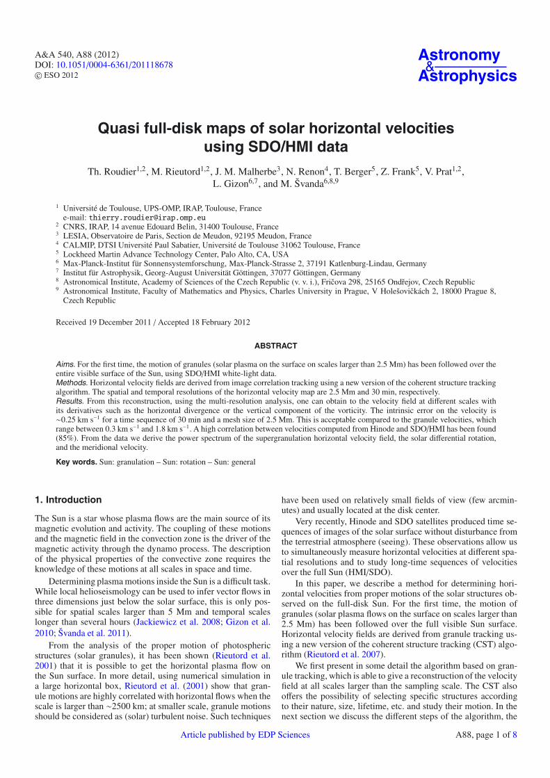
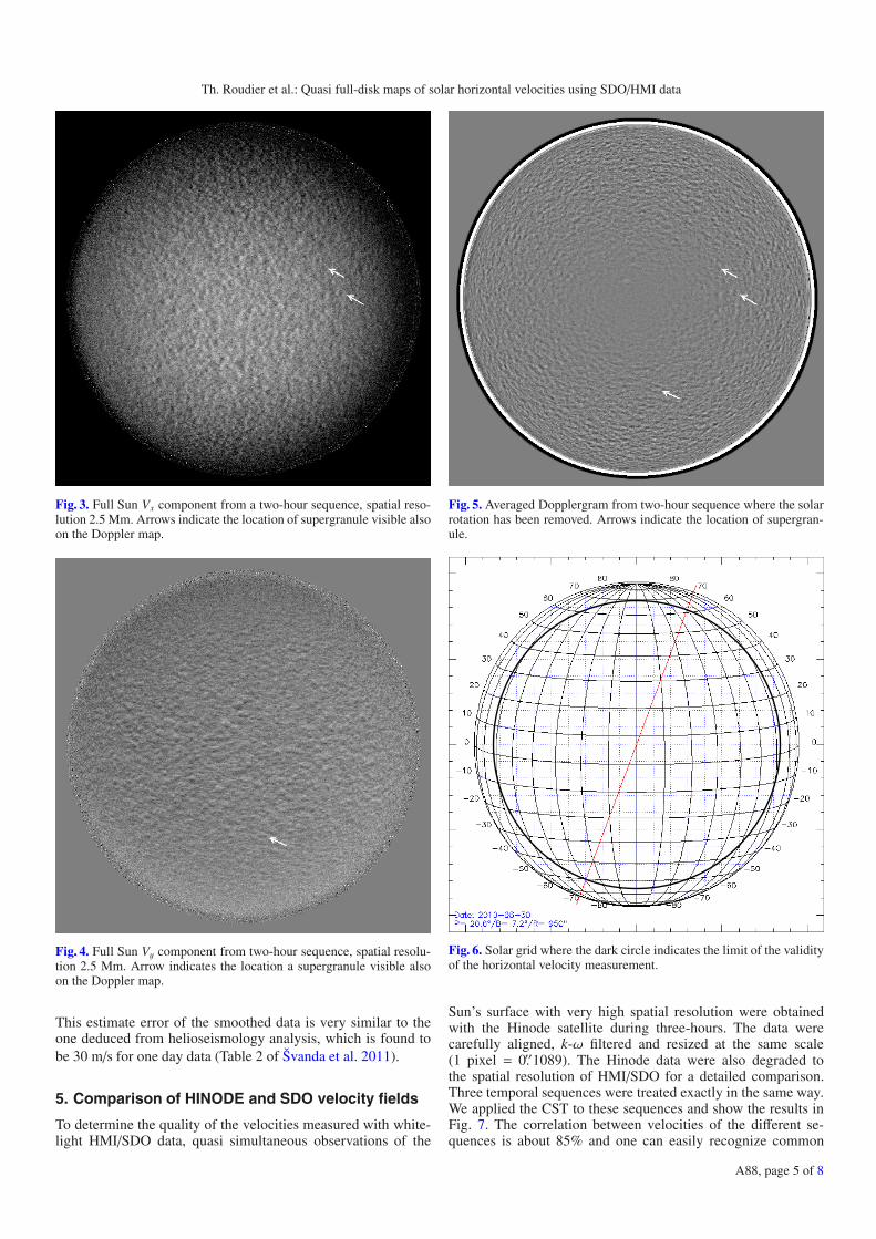
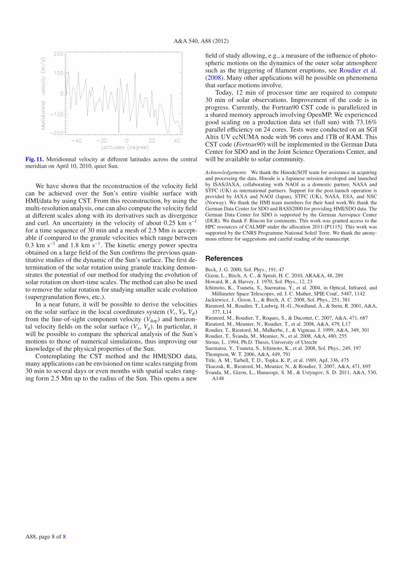
On the full Sun white-light observation around 5× 105 gran-ules are detected. During a time tracking of 30 min around2.2 × 106 coherent structures are identified. This number in-creases up to 7.5 × 106 for a time sequence of two-hours. Weshow an example of the full Sun Vx and Vy in Figs. 3 and 4components from a two-hour sequence with a spatial resolutionof 2.5 Mm. Arrows indicate the location of supergranules thatare visible also on the Doppler map (Fig. 5). Owing to the ra-dial flows within supergranules, two supergranules are markedin the Vx map close to the western limb where they are easier toidentify than in the east-west component of the flow (and viceversa for the Vy map). The circle inside the solar grid in Fig. 6represents the limit up to which the projected Vx and Vy are cor-rectly measured. Beyond this circle, granule tracking is difficultand errors increase rapidly as we near the limb. The useful fieldlies in the latitude and longitude range between ±60◦ in latitudeand longitude for a two-hour sequence. Because this field coversa large part of the visible Sun area (80%), we define it as a quasifull-disk map of photospheric horizontal velocities.

4. Precision

Following Tkaczuk et al. (2007), we can estimate the error prop-agation on the velocity of the CST algorithm. Over an image,granules are much less dense than pixels, therefore the velocityfield is sampled on a much coarser grid whose elements are of

A88, page 3 of 8

A&A 540, A88 (2012)

Fig. 2. Close-up view of the field around a spot as delineated in Fig. 1 (top left) with its segmentation (top right). Below, resulting velocity fieldfrom granule tracking (note the clear signature of the moat flow associated with the spot near x = 50, y = 100).

size δ here 2.5 Mm. The velocity at a grid coordinate (x, y) isassumed to be the average of the velocity of granules whose av-erage coordinates belong to the domain D around (x, y) (i.e. in[x−δ/2, x+δ/2], [y−δ/2, y+δ/2]). The spatial resolution of thevelocity field is given by the mesh size δ. If we assume that thedispersion on the barycenter is the same for the whole time series(σ), and that the time interval Δtk (of the granule k) is the samefor all granules (i.e. all granules have the same lifetime Δt), thenthe expression of the dispersion of the average velocity (Tkaczuket al. 2007) is

δV =

√2σ√NΔt, (1)

where N is the number of trajectories falling in D. We foundfor the full Sun white-light SDO data for a time sequence of30 min and a mesh size of 2.5 Mm, that N = 8. The precisionof the location of the barycenter of granule is estimated to half apixel, which represents 0.′′25 (183 km). With a median lifetimeof 405 s δV = 0.22 km s−1, which is good enough at a scale of

2500 km, i.e. at the scale where granule motion traces the large-scale plasma flows. Tkaczuk et al. (2007) showed that precisevelocity values need many granules in a grid element and a long-time interval. In other words, errors are less if a coarse resolutionin space and time is used.

When moving to the limb, the detection of granules be-comes more difficult but the mesh size δ covers a larger areaon the Sun’s surface. Both phenomena more or less canceleach other out and we find that close to the limb N = 7 andδV = 0.24 km s−1.

Accordingly, we estimate that an error of δV = 0.25 km s−1

for the HMI/SDO data for a time sequence of 30 min is accept-able since most of the granules are showing velocities in therange 0.3–1.8 km s−1 in our analysis. This error seems to belarge, but this is due in great part to the pixel size 0.′′5, whichallows us to follow only the large granules on the Sun surface.However, when the velocities are averaged in space and time thiserror decreases for example down to 0.06 km s−1 at the disk cen-ter with a window of 20′′ × 20′′ for a 24-h sequence (see below).

A88, page 4 of 8

Th. Roudier et al.: Quasi full-disk maps of solar horizontal velocities using SDO/HMI data

Fig. 3. Full Sun Vx component from a two-hour sequence, spatial reso-lution 2.5 Mm. Arrows indicate the location of supergranule visible alsoon the Doppler map.

Fig. 4. Full Sun Vy component from two-hour sequence, spatial resolu-tion 2.5 Mm. Arrow indicates the location a supergranule visible alsoon the Doppler map.

This estimate error of the smoothed data is very similar to theone deduced from helioseismology analysis, which is found tobe 30 m/s for one day data (Table 2 of Švanda et al. 2011).

5. Comparison of HINODE and SDO velocity fields

To determine the quality of the velocities measured with white-light HMI/SDO data, quasi simultaneous observations of the

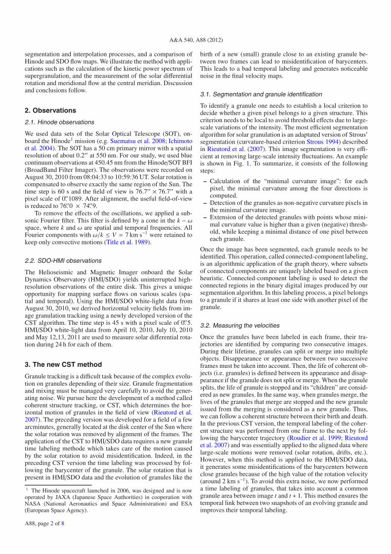
Fig. 5. Averaged Dopplergram from two-hour sequence where the solarrotation has been removed. Arrows indicate the location of supergran-ule.

Fig. 6. Solar grid where the dark circle indicates the limit of the validityof the horizontal velocity measurement.

Sun’s surface with very high spatial resolution were obtainedwith the Hinode satellite during three-hours. The data werecarefully aligned, k-ω filtered and resized at the same scale(1 pixel = 0.′′1089). The Hinode data were also degraded tothe spatial resolution of HMI/SDO for a detailed comparison.Three temporal sequences were treated exactly in the same way.We applied the CST to these sequences and show the results inFig. 7. The correlation between velocities of the different se-quences is about 85% and one can easily recognize common

A88, page 5 of 8

A&A 540, A88 (2012)

Fig. 7. Solar granulation from Hinode (1 pixel = 0.′′1089) on August 30,2010 8h04mn33s (top left) and horizontal velocities from a one-hoursequence (top right). Solar granulation from SDO (1 pixel = 0.′′5042),on August 30, 2010 8h04mn30s (middle left) and horizontal veloci-ties from a one-hour sequence (middle right). Solar granulation fromHinode degraded to a pixel of 0.′′5 on August 30, 2010 8h04mn30s (bot-tom left) and horizontal velocities from a one-hour sequence (bottomright).

patterns between the time series. The histograms of the veloc-ity in Fig. 8 are very similar for all sequence, indicating that theamplitudes are also correctly measured. For comparison, localcorrelation tracking (LCT) was applied to the same one-hour se-quence. This flow field is shown in the bottom of Fig. 7. Herewe also find a good correlation (about 75%) between velocitiescomputed by CST and LCT. The LCT velocities are lower, how-ever than the CST velocities by 15%, likely because of the spatialwindow size used in the LCT to convolve the data (Roudier et al.1999).

The high correlation between velocities and the quasi-identical amplitudes of the velocities indicate a good agreement

Fig. 8. Velocity histograms from CST and LCT are plotted in Fig. 7.

between velocities measured with Hinode data (high spatialresolution) and HMI/SDO data (low spatial resolution). This al-lows us to use HMI/SDO data with some confidence in deter-mining the horizontal flows across the Sun.

6. Power spectrum of the solar supergranulation

The kinetic energy distribution among the scales is representedby the power spectrum of the velocity field. Like Rieutord et al.(2008), we computed the kinetic energy spectral density E(k)for a time window of 120 min and spatial field of 650′′ × 650′′centered on the disk center on August 30, 2010.

The spectrum shown in Fig. 10 is very similar to that exhib-ited in Fig. 2 of Rieutord et al. (2008). It exhibits the kinetic en-ergy contained in the supergranulation. With SDO data, we findthe maximum of the spectral density at a wavelength of 35.8 Mmquite close to 36 Mm found by Rieutord et al. (2008) and theFWHM of the peak indicates that supergranulation occupies therange of scales of [19, 56] Mm compared to [20, 75] Mm forRieutord et al. (2008). Our time sequence is shorter by a factor3.75 but our field of view is 3.5 larger (400′′ ×300′′ for Rieutordet al. 2008). Like Rieutord et al., we indicate the best-fit power-law (3 and –2), which mimics the sides of the supergranulationspectral peak. At small scales below k = 0.1 Mm−1 we observeE(k) ∝ k due to the decorrelated random noise. Our present re-sult confirms the previous findings.

7. Solar differential and meridional flowdetermination

There is a long history of inconsistent measurements of solar ro-tation (Beck 2000). One of the first applications of the CST algo-rithm on HMI/SDO data is to measure the horizontal velocitiesover 24 h on the central meridian. Owing to computational time,we used a band of 50′′ along the central meridian and 48 time-sequences of 30 min. Then, 98 spatial windows of 50′′ × 20′′were used to obtain the horizontal flow fields at different lati-tudes for each time-sequence of 30 min. Finally, we averagedall 30 min time-sequences for each latitude to obtain the finalVx and Vy over 24 h. The Vx are corrected for the Earth’s orbitalmotion to obtain the sidereal rotation of the Sun, and Vy was alsocorrected for the B0 evolution during 24 h. This is the first timethat solar rotation has been determined from granule displace-ment measurements over the full solar disk. Figure 9 shows thedifferential rotation computed in this way for four different datesclose to the solar minimum.

The standard deviation of the velocity field close to the diskcenter is 0.06 km s−1 (24 h sequence). Owing to the change in

A88, page 6 of 8

Th. Roudier et al.: Quasi full-disk maps of solar horizontal velocities using SDO/HMI data

Fig. 9. Solar differential rotation on April 10, 2010, July 10, 2010, May 12, 2011, and May 13, 2011. We plot the rotation law determined byspectroscopic method (Howard & Harvey 1970) in the four panels ω = 13.76−1.74 × sin2 λ − 2.19 × sin4 λ (λ = latitude, ω = angular velocity indeg/day), giving an equatorial velocity of 1.93 km s−1.

size of the Sun in diameter of (1.4 pixel on the detector) (SDOEarth orbit) and also to the B0 evolution during 24 h, the fieldof good measurement was reduced to −50◦ and +45◦ in longi-tude and ±50◦ in latitude around the disk center. This limita-tion will be improved in the near future (new observations on10 December 2011) by reducing the effects of dilatation and con-traction of the Sun’s diameter on the CCD.

Our results of April 10, 2010 agree with the spectroscopicdetermination of the solar rotation of Howard & Harvey (1970)but the rotation seems slightly faster on the other dates with anequatorial velocity of 1.99 km s−1. The daily Wolf numbers are8, 14, 33, and 26 and 8, 16.1, and 41.6 monthly. We expect dif-ferences with Howard & Harvey (1970), simply because we arenot studying the same time period. The solar differential rotationappears to change in time particularly at high latitudes, but weneed a more extensive analysis to confirm these variations.

The meridional flows with Vrms = 90 m s−1, given by theVy component for 24 h, is plotted in Fig. 11 for a quiet Sun onApril 10 2010 between −50◦ and +45◦ in latitude. Because theVrms of the mean meridional flow is 90 m s−1, the expected signalof 20 m s−1 is completely hidden. Several days are required toreduce the Vrms amplitude and determine the meridional veloc-ity. This work is scheduled for the near future because we mustalso include the Sun’s diameter evolution on the SDO detectorover a long period of time (Earth orbit).

8. Discussion and conclusions

Determining horizontal velocity fields on the solar surface iscrucial for understanding the dynamics of the phostosphere, the

Fig. 10. Kinetic energy spectra of the horizontal velocities. The verticaldashed line emphasizes the 10 Mm scale, which is usually taken asupper limit of mesogranular scale. Two power laws are shown on eachside of the peak, as well as that of the small-scale noise.

distribution of magnetic fields and its influence on the structuresof the solar atmosphere (filaments, jets, etc.).

A88, page 7 of 8

A&A 540, A88 (2012)

Fig. 11. Meridionnal velocity at different latitudes across the centralmeridian on April 10, 2010, quiet Sun.

We have shown that the reconstruction of the velocity fieldcan be achieved over the Sun’s entire visible surface withHMI/data by using CST. From this reconstruction, by using themulti-resolution analysis, one can also compute the velocity fieldat different scales along with its derivatives such as divergenceand curl. An uncertainty in the velocity of about 0.25 km s−1

for a time sequence of 30 min and a mesh of 2.5 Mm is accept-able if compared to the granule velocities which range between0.3 km s−1 and 1.8 km s−1. The kinetic energy power spectraobtained on a large field of the Sun confirms the previous quan-titative studies of the dynamic of the Sun’s surface. The first de-termination of the solar rotation using granule tracking demon-strates the potential of our method for studying the evolution ofsolar rotation on short-time scales. The method can also be usedto remove the solar rotation for studying smaller scale evolution(supergranulation flows, etc.).

In a near future, it will be possible to derive the velocitieson the solar surface in the local coordinates system (Vr,Vθ,Vφ)from the line-of-sight component velocity (Vdop) and horizon-tal velocity fields on the solar surface (Vx, Vy). In particular, itwill be possible to compare the spherical analysis of the Sun’smotions to those of numerical simulations, thus improving ourknowledge of the physical properties of the Sun.

Contemplating the CST method and the HMI/SDO data,many applications can be envisioned on time scales ranging from30 min to several days or even months with spatial scales rang-ing form 2.5 Mm up to the radius of the Sun. This opens a new

field of study allowing, e.g., a measure of the influence of photo-spheric motions on the dynamics of the outer solar atmospheresuch as the triggering of filament eruptions, see Roudier et al.(2008). Many other applications will be possible on phenomenathat surface motions involve.

Today, 12 min of processor time are required to compute30 min of solar observations. Improvement of the code is inprogress. Currently, the Fortran90 CST code is parallelized ina shared memory approach involving OpenMP. We experiencedgood scaling on a production data set (full sun) with 73.16%parallel efficiency on 24 cores. Tests were conducted on an SGIAltix UV ccNUMA node with 96 cores and 1TB of RAM. ThisCST code (Fortran90) will be implemented in the German DataCenter for SDO and in the Joint Science Operations Center, andwill be available to solar community.

Acknowledgements. We thank the Hinode/SOT team for assistance in acquiringand processing the data. Hinode is a Japanese mission developed and launchedby ISAS/JAXA, collaborating with NAOJ as a domestic partner, NASA andSTFC (UK) as international partners. Support for the post-launch operation isprovided by JAXA and NAOJ (Japan), STFC (UK), NASA, ESA, and NSC(Norway). We thank the HMI team members for their hard work.We thank theGerman Data Center for SDO and BASS2000 for providing HMI/SDO data. TheGerman Data Center for SDO is supported by the German Aerospace Center(DLR). We thank F. Rincon for comments. This work was granted access to theHPC resources of CALMIP under the allocation 2011-[P1115]. This work wassupported by the CNRS Programme National Soleil Terre. We thank the anony-mous referee for suggestions and careful reading of the manuscript.

References

Beck, J. G. 2000, Sol. Phys., 191, 47Gizon, L., Birch, A. C., & Spruit, H. C. 2010, ARA&A, 48, 289Howard, R., & Harvey, J. 1970, Sol. Phys., 12, 23Ichimoto, K., Tsuneta, S., Suematsu, Y., et al. 2004, in Optical, Infrared, and

Millimeter Space Telescopes, ed. J. C. Mather, SPIE Conf., 5487, 1142Jackiewicz, J., Gizon, L., & Birch, A. C. 2008, Sol. Phys., 251, 381Rieutord, M., Roudier, T., Ludwig, H.-G., Nordlund, Å., & Stein, R. 2001, A&A,

377, L14Rieutord, M., Roudier, T., Roques, S., & Ducottet, C. 2007, A&A, 471, 687Rieutord, M., Meunier, N., Roudier, T., et al. 2008, A&A, 479, L17Roudier, T., Rieutord, M., Malherbe, J., & Vigneau, J. 1999, A&A, 349, 301Roudier, T., Švanda, M., Meunier, N., et al. 2008, A&A, 480, 255Strous, L. 1994, Ph.D. Thesis, University of UtrechtSuematsu, Y., Tsuneta, S., Ichimoto, K., et al. 2008, Sol. Phys., 249, 197Thompson, W. T. 2006, A&A, 449, 791Title, A. M., Tarbell, T. D., Topka, K. P., et al. 1989, ApJ, 336, 475Tkaczuk, R., Rieutord, M., Meunier, N., & Roudier, T. 2007, A&A, 471, 695Švanda, M., Gizon, L., Hanasoge, S. M., & Ustyugov, S. D. 2011, A&A, 530,

A148

A88, page 8 of 8