Assumption checking in “normal” multiple regression with Stata.
12
Assumption checking in “normal” multiple regression with Stata
-
Upload
ethelbert-tucker -
Category
Documents
-
view
237 -
download
0
Transcript of Assumption checking in “normal” multiple regression with Stata.

Assumption checking in “normal” multiple regression
with Stata

2
Assumptions in regression analysis•No multi-collinearity
•All relevant predictor variables included•Homoscedasticity: all residuals are from a distribution with the same variance•Linearity: the “true” model should be linear.•Independent errors: having information about the value of a residual should not give you information about the value of other residuals•Errors are distributed normally
3
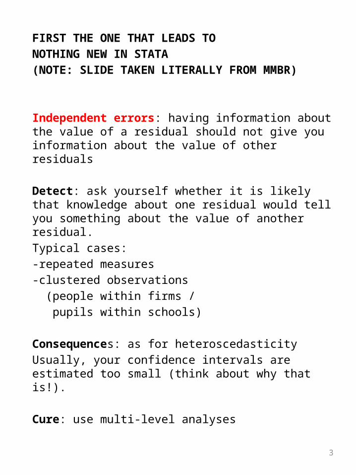
FIRST THE ONE THAT LEADS TO NOTHING NEW IN STATA (NOTE: SLIDE TAKEN LITERALLY FROM MMBR)
Independent errors: having information about the value of a residual should not give you information about the value of other residuals
Detect: ask yourself whether it is likely that knowledge about one residual would tell you something about the value of another residual.Typical cases:
-repeated measures-clustered observations (people within firms / pupils within schools)
Consequences: as for heteroscedasticityUsually, your confidence intervals are estimated too small (think about why that is!).
Cure: use multi-level analyses
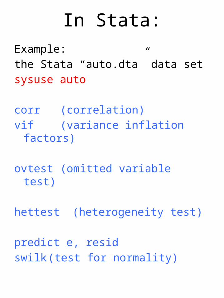
In Stata:
Example: the Stata “auto.dta” data setsysuse auto
corr (correlation)vif (variance inflation
factors)
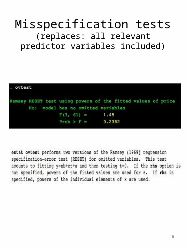
ovtest (omitted variable test)
hettest (heterogeneity test)
predict e, residswilk (test for normality)
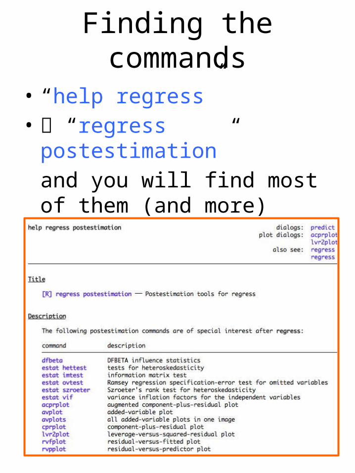
Finding the commands
• “help regress”• “regress postestimation”
and you will find most of them (and more) there
6
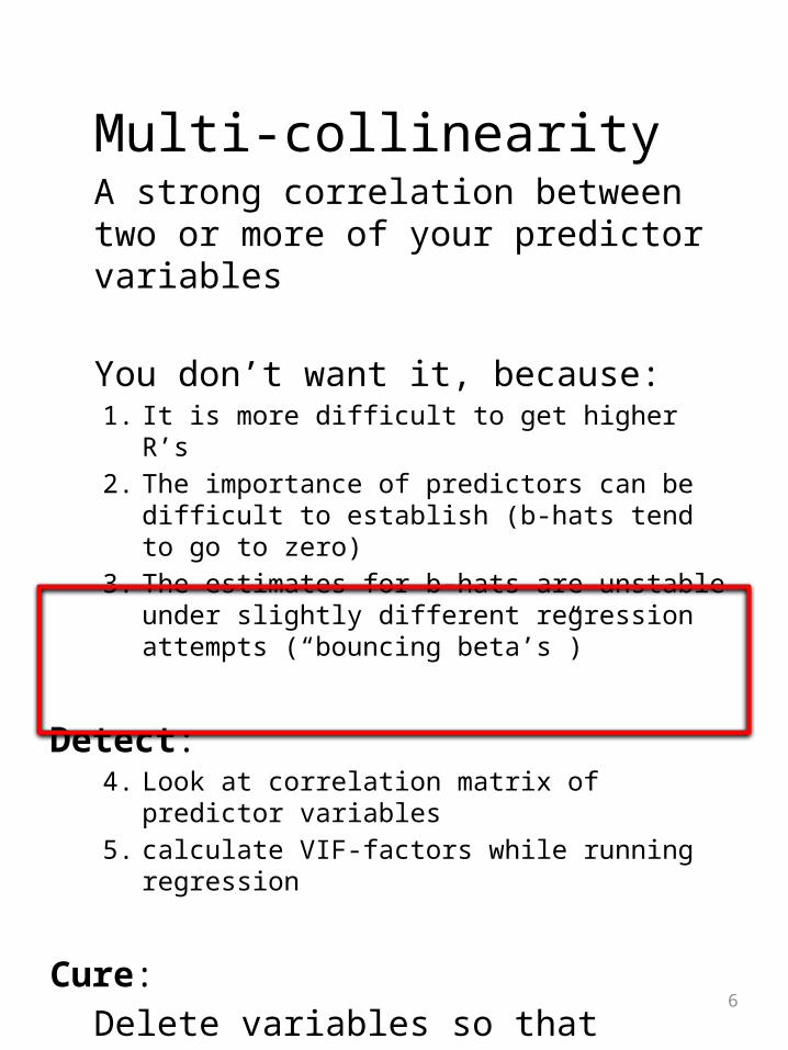
Multi-collinearity A strong correlation between two or more of your predictor variables
You don’t want it, because:1. It is more difficult to get higher R’s2. The importance of predictors can be difficult to
establish (b-hats tend to go to zero)3. The estimates for b-hats are unstable under slightly
different regression attempts (“bouncing beta’s”)
Detect: 4. Look at correlation matrix of predictor variables5. calculate VIF-factors while running regression
Cure:Delete variables so that multi-collinearity disappears, for instance by combining them into a single variable
7
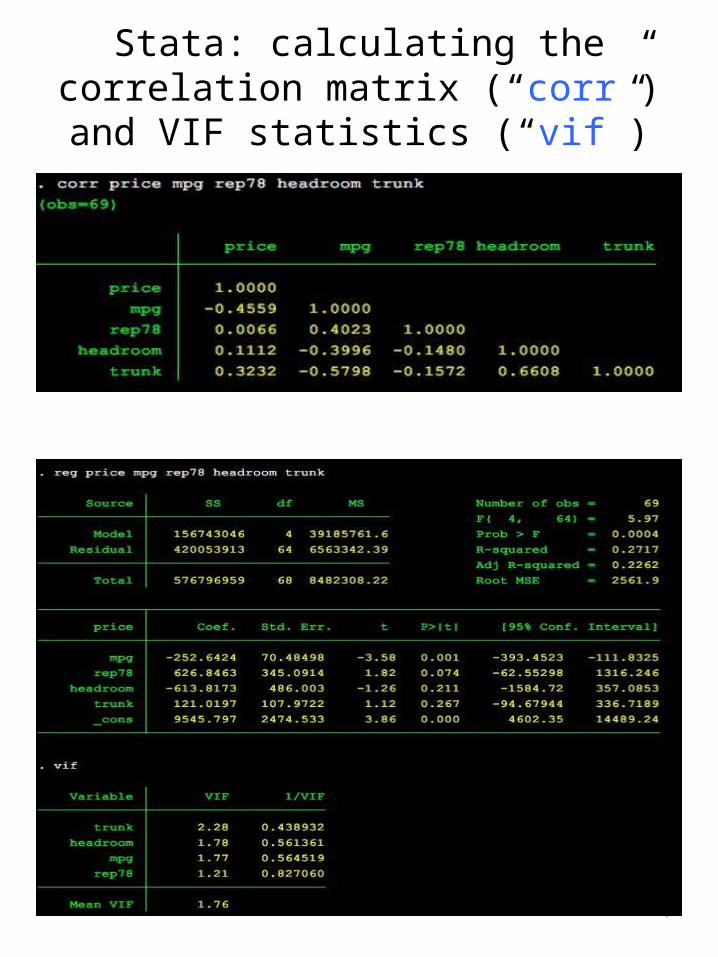
Stata: calculating the correlation matrix (“corr”) and VIF statistics (“vif”)
8
Misspecification tests(replaces: all relevant predictor
variables included)
9
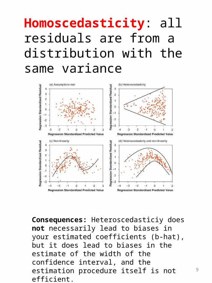
Homoscedasticity: all residuals are from a distribution with the same variance
Consequences: Heteroscedasticiy does not necessarily lead to biases in your estimated coefficients (b-hat), but it does lead to biases in the estimate of the width of the confidence interval, and the estimation procedure itself is not efficient.
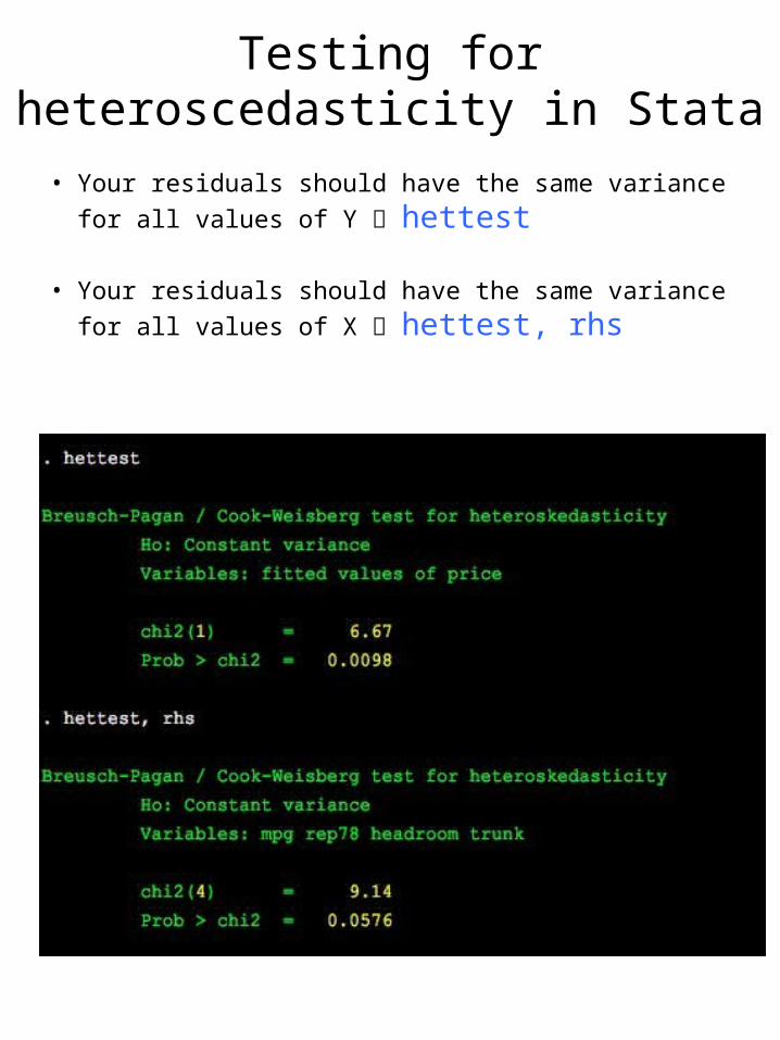
Testing for heteroscedasticity in Stata
• Your residuals should have the same variance for all values of Y hettest
• Your residuals should have the same variance for all values of X hettest, rhs
11
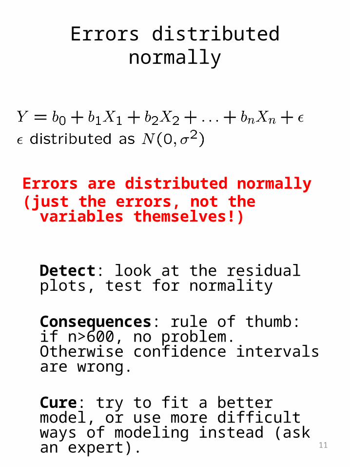
Errors distributed normally
Errors are distributed normally (just the errors, not the variables themselves!)
Detect: look at the residual plots, test for normality
Consequences: rule of thumb: if n>600, no problem. Otherwise confidence intervals are wrong.
Cure: try to fit a better model, or use more difficult ways of modeling instead (ask an expert).
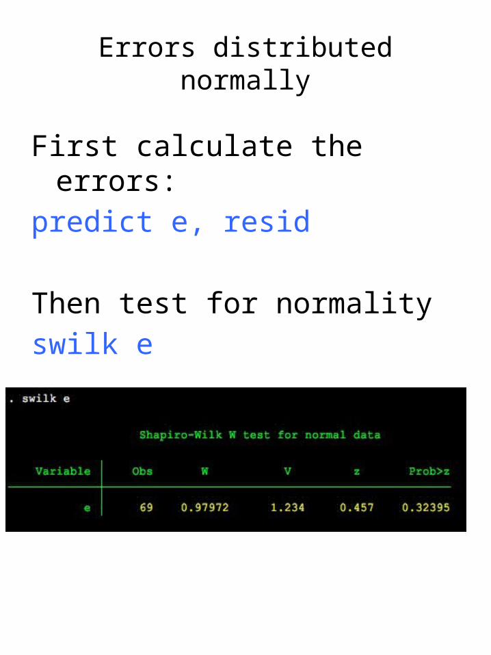
First calculate the errors:predict e, resid
Then test for normalityswilk e
Errors distributed normally

![[ME] Multilevel Mixed Effects - Survey Design · 2016. 2. 16. · Stata, , Stata Press, Mata, , and NetCourse are registered trademarks of StataCorp LP. Stata and Stata Press are](https://static.fdocuments.us/doc/165x107/6119d35ebac5e41ff76887ce/me-multilevel-mixed-effects-survey-design-2016-2-16-stata-stata-press.jpg)