Panel Data Analysis - Amine Ouazad · Balanced panel data • Balanced panel data: ... • Checking...

Panel Data Analysis

Econometrics AAss. Prof. Amine Ouazad

Tuesday, March 6, 12

References• William H. Greene, Chapter on Models

for Panel Data.

• Quarterly Journal of Economics, “Managing with Style: The Effect of Managers on Firm Policies”, November 2003.

2


Outline1. Panel data examples2. Cross-section vs longitudinal analysis3. Fixed effects estimation– OLS, within, first-differenced estimator

4. Random effects estimation5. Hausman test6. Tricky questions7. Two way fixed effects regression


PANEL DATA EXAMPLES


Panel data examples• Active workers followed term after

term. Labor Force Survey.– Calculation of the unemployment rate.

• Families’ purchasing decision followed over multiple weeks.– Consumer Expenditure Survey.

• Firms’ share prices/earnings/accounting measures.– Compustat + Execucomp.


Panel data notation• i: individual, firm, “unit” of analysis.• t: time period. Either minute, day,

hour, week, year, etc.• Sometimes individuals/firms are

grouped into units.– J(i,t): firm of employee i at time t.

6


Cross sectionvs longitudinal data analysis

• In cross-sectional regressions, individuals differ both in their covariates and in constant unobservable dimensions.

• In longitudinal regressions, where changes in the outcome variable are related to changes in the covariates, the non time-varying unobservables are captured.


Usefulness of panel data analysis

1. Capture non-time varying unobservables.

2. Correct for individual or time-specific unobserved shocks.

3. Estimate non-time varying unobservables, their correlation with observables, their significance.

8


FIXED EFFECTS ESTIMATION


yi = Xi� + i · ↵i + "i

yi,t = x

0i,t� + ↵i + "i,t

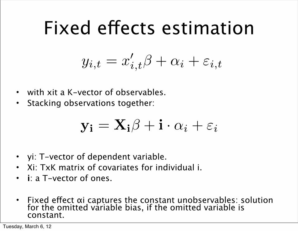
Fixed effects estimation

• with xit a K-vector of observables.• Stacking observations together:

• yi: T-vector of dependent variable.• Xi: TxK matrix of covariates for individual i.• i: a T-vector of ones.

• Fixed effect αi captures the constant unobservables: solution for the omitted variable bias, if the omitted variable is constant.


Balanced panel data• Balanced panel data:

– Same number of time periods T of observation for each individual i=1,2,..,N.

• Unbalanced panel data:– At least one individual is observed for a different number of time

periods. – Ti : number of observations for individual i.

• Checking in Stata: using xtset.

• If Ti is random (non correlated with epsilon i), then the unbalancedness is not an issue. Most results of this session apply.

• If Ti is nonrandom, there is either:– endogenous entry into the dataset.– Or endogenous exit (attrition) out of the dataset.

• Then specific theory needs to be developed(out of the scope of the current session).

11


y = X� +D↵+ "

Matrix form

• X is an NT times K matrix.• D is an NT times N matrix, the design matrix.• alpha: an N-vector of fixed effects.• The constant is either in X, and then D drops one

effect, or the constant is in D, and then X has no constant. The former is the typical convention.

12


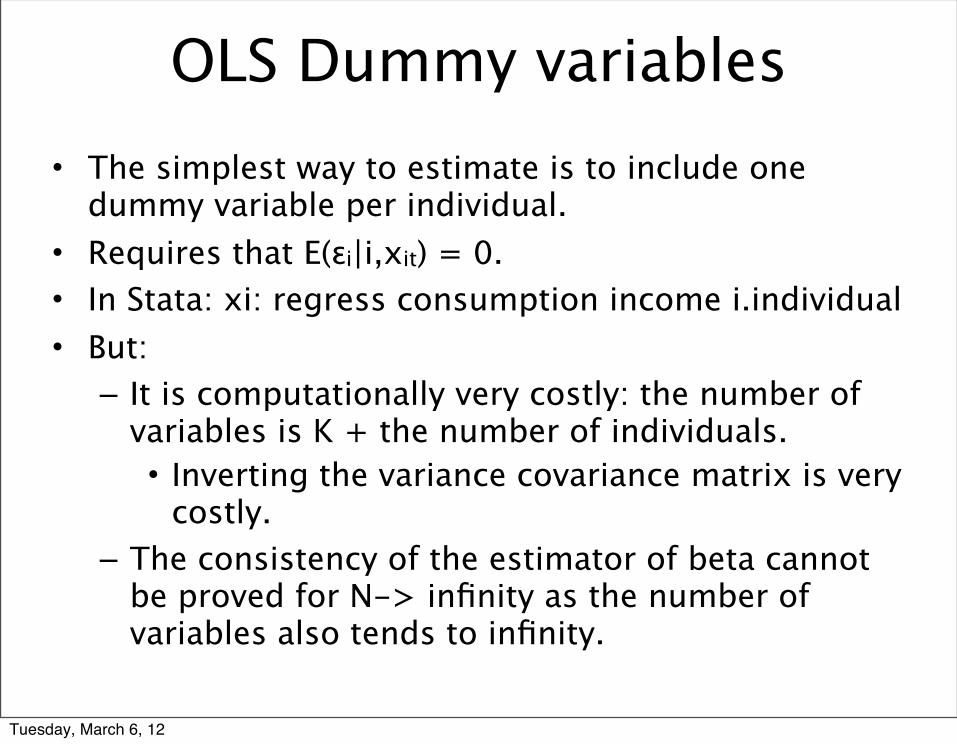
OLS Dummy variables • The simplest way to estimate is to include one

dummy variable per individual.• Requires that E(εi|i,xit) = 0.• In Stata: xi: regress consumption income i.individual • But:– It is computationally very costly: the number of

variables is K + the number of individuals.• Inverting the variance covariance matrix is very

costly.– The consistency of the estimator of beta cannot

be proved for N-> infinity as the number of variables also tends to infinity.


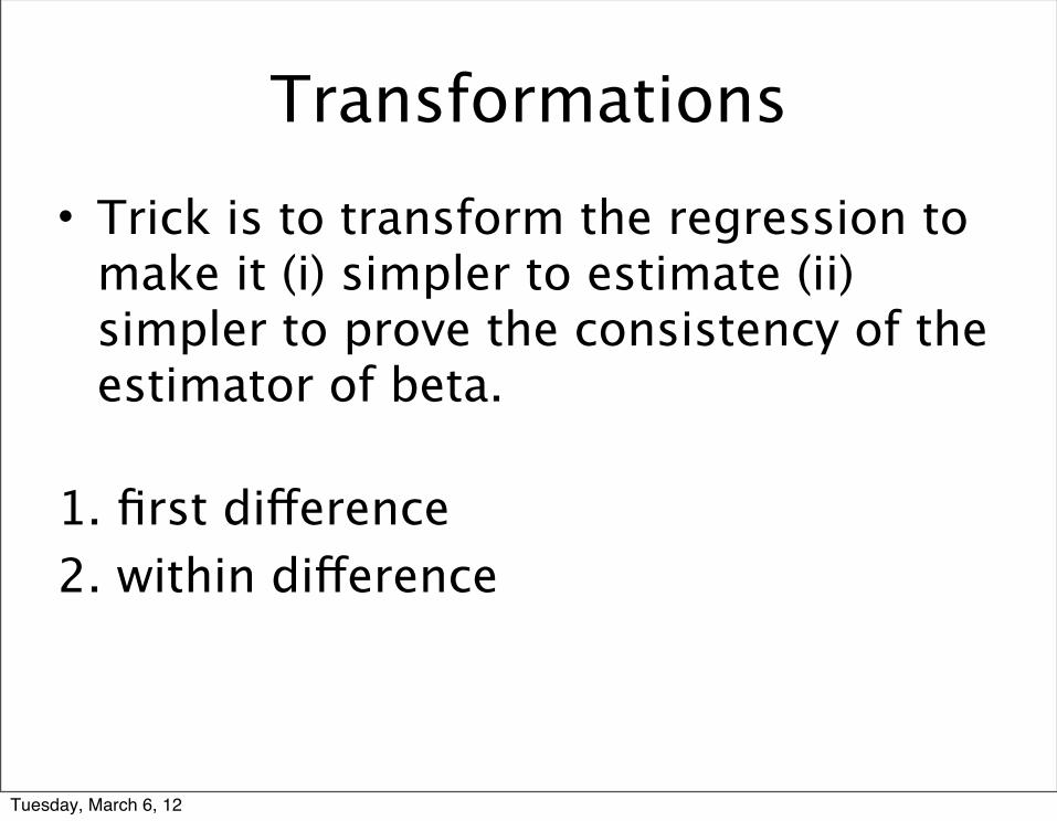
Transformations• Trick is to transform the regression to

make it (i) simpler to estimate (ii) simpler to prove the consistency of the estimator of beta.

1. first difference2. within difference


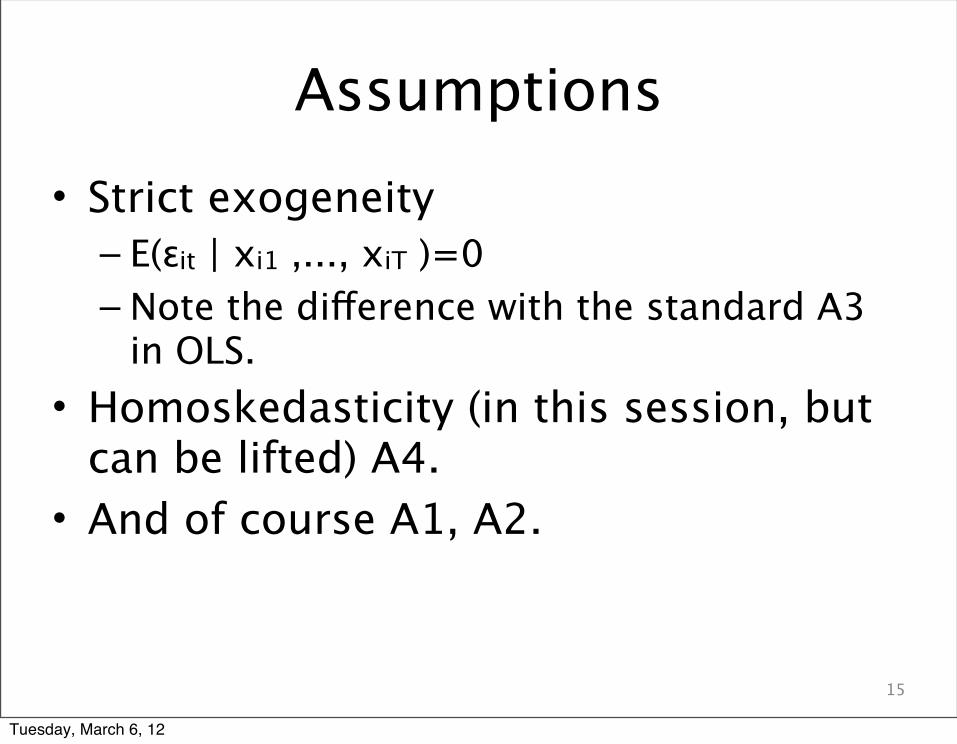
Assumptions• Strict exogeneity– E(εit | xi1 ,..., xiT )=0– Note the difference with the standard A3

in OLS.• Homoskedasticity (in this session, but

can be lifted) A4.• And of course A1, A2.

15


yi,t � yi,t�1 = (xi,t � xi,t�1)0� + "i,t � "i,t�1

First-differenced estimator

• Note that strict exogeneity implies that A3 is satisfied for this first-differenced regression.

• Noting ∆ the first-differenced estimator.

• In vector form.

16

�yi = �xi0� +�"i


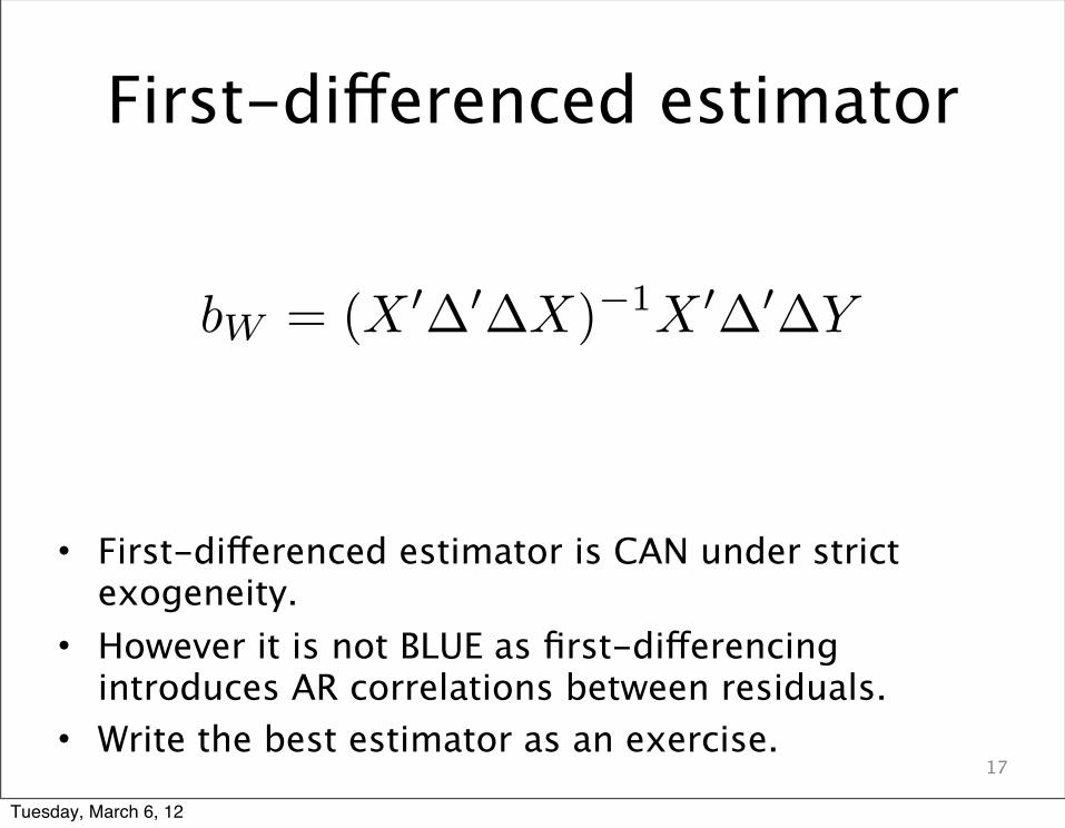
bW = (X 0�0�X)�1X 0�0�Y

First-differenced estimator

• First-differenced estimator is CAN under strict exogeneity.

• However it is not BLUE as first-differencing introduces AR correlations between residuals.

• Write the best estimator as an exercise.17


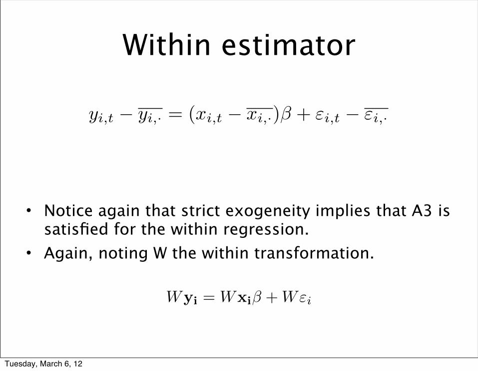
yi,t � yi,· = (xi,t � xi,·)� + "i,t � "i,·

Wyi = Wxi� +W"i

Within estimator

• Notice again that strict exogeneity implies that A3 is satisfied for the within regression.

• Again, noting W the within transformation.


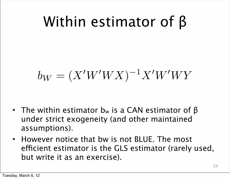
Within estimator of β

• The within estimator bw is a CAN estimator of β under strict exogeneity (and other maintained assumptions).

• However notice that bw is not BLUE. The most efficient estimator is the GLS estimator (rarely used, but write it as an exercise).

19

bW = (X 0W 0WX)�1X 0W 0WY


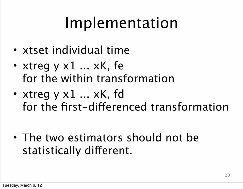
Implementation• xtset individual time• xtreg y x1 ... xK, fe

for the within transformation• xtreg y x1 ... xK, fd

for the first-differenced transformation

• The two estimators should not be statistically different.

20


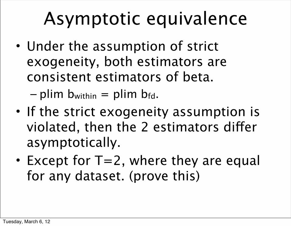
Asymptotic equivalence• Under the assumption of strict

exogeneity, both estimators are consistent estimators of beta.– plim bwithin = plim bfd.

• If the strict exogeneity assumption is violated, then the 2 estimators differ asymptotically.

• Except for T=2, where they are equal for any dataset. (prove this)


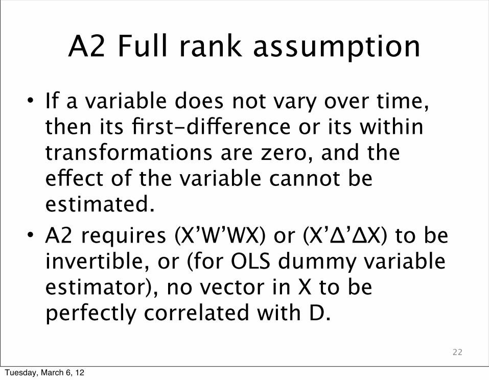
A2 Full rank assumption• If a variable does not vary over time,

then its first-difference or its within transformations are zero, and the effect of the variable cannot be estimated.

• A2 requires (X’W’WX) or (X’Δ’ΔX) to be invertible, or (for OLS dummy variable estimator), no vector in X to be perfectly correlated with D.

22


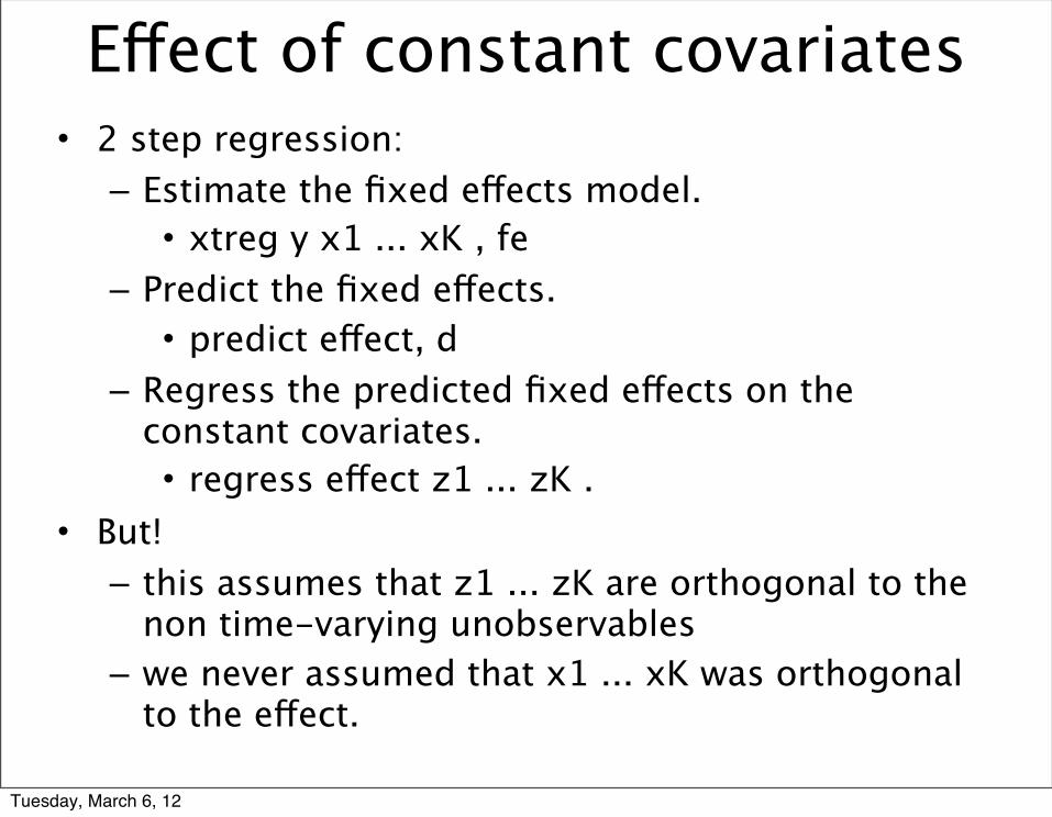
Effect of constant covariates• 2 step regression:– Estimate the fixed effects model.• xtreg y x1 ... xK , fe

– Predict the fixed effects.• predict effect, d

– Regress the predicted fixed effects on the constant covariates.• regress effect z1 ... zK .

• But!– this assumes that z1 ... zK are orthogonal to the

non time-varying unobservables– we never assumed that x1 ... xK was orthogonal

to the effect.


Do not• Perform the transformation yourself

and report the standard errors of the regression.– The s.e.s would be wrong.

• Rather, let stata do the correction on the standard errors for you.

24


IV regression and fixed effects

• IV estimation can be combined with a fixed effect regression.

• IV will take care (if valid) of the time-varying unobservables.

• Hence IV needs to be time varying.• Stata command xtivreg/xtivreg2.


Fixed effects regression and measurement error

• Fixed effects regression tends in general to magnify measurement error.

• In the first-differenced estimator:– The variance of the first-differenced

transformation is typically smaller than the variance of the levels. Exercise.

• In the within estimator:– The variance of the within-transformed

covariates is smaller than the original variance. Exercise.


RANDOM EFFECTS ESTIMATION


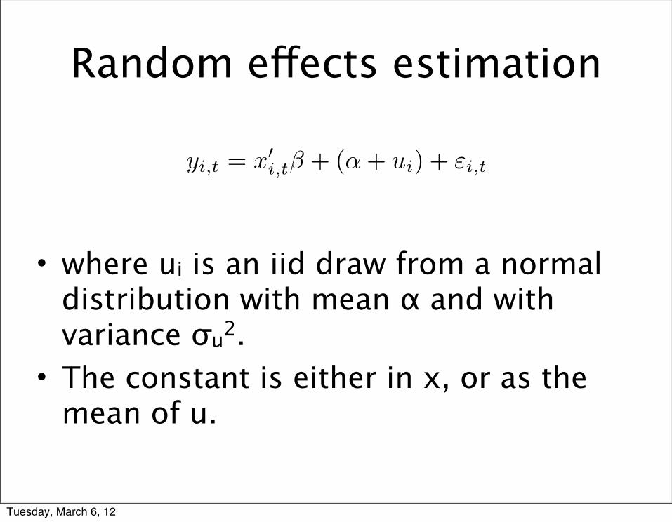
yi,t = x

0i,t� + (↵+ ui) + "i,t

Random effects estimation

• where ui is an iid draw from a normal distribution with mean α and with variance σu2.

• The constant is either in x, or as the mean of u.


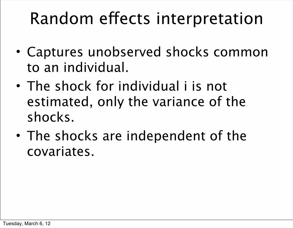
Random effects interpretation

• Captures unobserved shocks common to an individual.

• The shock for individual i is not estimated, only the variance of the shocks.

• The shocks are independent of the covariates.


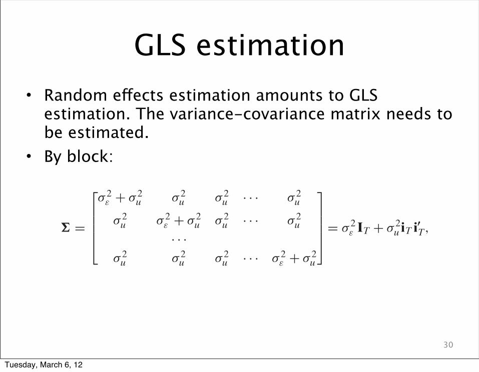
GLS estimation• Random effects estimation amounts to GLS

estimation. The variance-covariance matrix needs to be estimated.

• By block:

30

Greene-50240 book June 18, 2002 15:28

294 CHAPTER 13 ! Models for Panel Data

in the introduction to this chapter.10 The payoff to this form is that it greatly reducesthe number of parameters to be estimated. The cost is the possibility of inconsistentestimates, should the assumption turn out to be inappropriate.

Consider, then, a reformulation of the model

yit = x!i t! + (! + ui ) + "i t , (13-18)

where there are K regressors including a constant and now the single constant term isthe mean of the unobserved heterogeneity, E [z!

i"]. The component ui is the randomheterogeneity specific to the ith observation and is constant through time; recall fromSection 13.2, ui =

!

z!i" ! E [z!

i"]"

. For example, in an analysis of families, we can viewui as the collection of factors, z!

i", not in the regression that are specific to that family.We assume further that

E ["i t | X] = E [ui | X] = 0,

E#

"2i t

$

$X%

= # 2" ,

E#

u2i

$

$X%

= # 2u ,

E ["i t u j | X] = 0 for all i, t, and j,

E ["i t" js | X] = 0 if t "= s or i "= j,

E [ui u j | X] = 0 if i "= j.

(13-19)

As before, it is useful to view the formulation of the model in blocks of T observationsfor group i, yi , Xi , ui i, and #i . For these T observations, let

$i t = "i t + ui

and

$i = [$i1, $i2, . . . , $iT]#.

In view of this form of $i t , we have what is often called an “error components model.”For this model,

E#

$2i t

$

$X%

= # 2" + # 2

u ,

E [$i t$is | X] = # 2u , t "= s

E [$i t$ js | X] = 0 for all t and s if i "= j.

For the T observations for unit i , let % = E [$i$!i | X]. Then

% =

&

'

'

'

(

# 2" + # 2

u # 2u # 2

u · · · # 2u

# 2u # 2

" + # 2u # 2

u · · · # 2u

· · ·# 2

u # 2u # 2

u · · · # 2" + # 2

u

)

*

*

*

+

= # 2" IT + # 2

u iT i!T, (13-20)

10This distinction is not hard and fast; it is purely heuristic. We shall return to this issue later. See Mundlak(1978) for methodological discussion of the distinction between fixed and random effects.


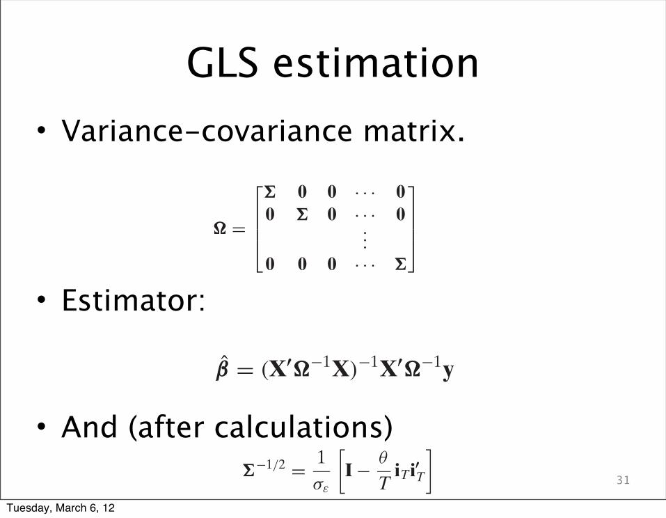
GLS estimation• Variance-covariance matrix.

• Estimator:

• And (after calculations)31

Greene-50240 book June 18, 2002 15:28

CHAPTER 13 ! Models for Panel Data 295

where iT is a T ! 1 column vector of 1s. Since observations i and j are independent, thedisturbance covariance matrix for the full nT observations is

! =

!

"

"

#

" 0 0 · · · 00 " 0 · · · 0

...

0 0 0 · · · "

$

%

%

&

= In " ". (13-21)

13.4.1 GENERALIZED LEAST SQUARES

The generalized least squares estimator of the slope parameters is

# = (X!!#1X)#1X!!#1y ='

n(

i=1

X!i!

#1Xi

)#1' n(

i=1

X!i!

#1yi

)

To compute this estimator as we did in Chapter 10 by transforming the data and usingordinary least squares with the transformed data, we will require !#1/2 = [In " "]#1/2.We need only find "#1/2, which is

"#1/2 = 1!"

*

I # #

TiTi!T

+

,

where

# = 1 # !",

! 2" + T! 2

u

.

The transformation of yi and Xi for GLS is therefore

"#1/2yi = 1!"

!

"

"

"

#

yı1 # # yı.

yı2 # # yı....

yıT # # yı.

$

%

%

%

&

, (13-22)

and likewise for the rows of Xi .11 For the data set as a whole, then, generalized leastsquares is computed by the regression of these partial deviations of yit on the sametransformations of xi t . Note the similarity of this procedure to the computation in theLSDV model, which uses # = 1. (One could interpret # as the effect that would remainif !" were zero, because the only effect would then be ui . In this case, the fixed andrandom effects models would be indistinguishable, so this result makes sense.)

It can be shown that the GLS estimator is, like the OLS estimator, a matrix weightedaverage of the within- and between-units estimators:

# = Fwithinbwithin + (I # Fwithin)bbetween,12 (13-23)

11This transformation is a special case of the more general treatment in Nerlove (1971b).12An alternative form of this expression, in which the weighing matrices are proportional to the covariancematrices of the two estimators, is given by Judge et al. (1985).

Greene-50240 book June 18, 2002 15:28



! =

!

"

"

#

" 0 0 · · · 00 " 0 · · · 0

...

0 0 0 · · · "

$

%

%

&

= In " ". (13-21)



# = (X!!#1X)#1X!!#1y ='

n(

i=1

X!i!

#1Xi

)#1' n(

i=1

X!i!

#1yi

)


"#1/2 = 1!"

*

I # #

TiTi!T

+

,

where

# = 1 # !",

! 2" + T! 2

u

.


"#1/2yi = 1!"

!

"

"

"

#

yı1 # # yı.

yı2 # # yı....

yıT # # yı.

$

%

%

%

&

, (13-22)





Greene-50240 book June 18, 2002 15:28



! =

!

"

"

#

" 0 0 · · · 00 " 0 · · · 0

...

0 0 0 · · · "

$

%

%

&

= In " ". (13-21)



# = (X!!#1X)#1X!!#1y ='

n(

i=1

X!i!

#1Xi

)#1' n(

i=1

X!i!

#1yi

)


"#1/2 = 1!"

*

I # #

TiTi!T

+

,

where

# = 1 # !",

! 2" + T! 2

u

.


"#1/2yi = 1!"

!

"

"

"

#

yı1 # # yı.

yı2 # # yı....

yıT # # yı.

$

%

%

%

&

, (13-22)






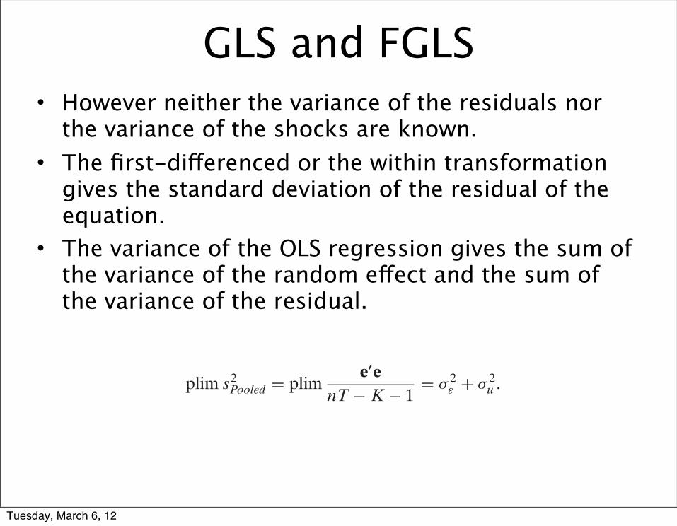
GLS and FGLS• However neither the variance of the residuals nor

the variance of the shocks are known.• The first-differenced or the within transformation

gives the standard deviation of the residual of the equation.

• The variance of the OLS regression gives the sum of the variance of the random effect and the sum of the variance of the residual.

Greene-50240 book June 18, 2002 15:28


model with only a single overall constant, we have

plim s2Pooled = plim

e!enT ! K ! 1

= ! 2" + ! 2

u . (13-30)

This provides the two estimators needed for the variance components; the second wouldbe ! 2

u = s2Pooled ! s2

LSDV . A possible complication is that this second estimator could benegative. But, recall that for feasible generalized least squares, we do not need anunbiased estimator of the variance, only a consistent one. As such, we may drop thedegrees of freedom corrections in (13-29) and (13-30). If so, then the two varianceestimators must be nonnegative, since the sum of squares in the LSDV model cannotbe larger than that in the simple regression with only one constant term. Alternativeestimators have been proposed, all based on this principle of using two different sumsof squared residuals.14

There is a remaining complication. If there are any regressors that do not varywithin the groups, the LSDV estimator cannot be computed. For example, in a modelof family income or labor supply, one of the regressors might be a dummy variablefor location, family structure, or living arrangement. Any of these could be perfectlycollinear with the fixed effect for that family, which would prevent computation of theLSDV estimator. In this case, it is still possible to estimate the random effects variancecomponents. Let [b, a] be any consistent estimator of [!,#], such as the ordinary leastsquares estimator. Then, (13-30) provides a consistent estimator of mee = ! 2

" + ! 2u . The

mean squared residuals using a regression based only on the n group means provides aconsistent estimator of m"" = ! 2

u + (! 2" /T ), so we can use

! 2" = T

T ! 1(mee ! m"")

! 2u = T

T ! 1m"" ! 1

T ! 1mee = $m"" + (1 ! $)mee,

where $ > 1. As before, this estimator can produce a negative estimate of ! 2u that, once

again, calls the specification of the model into question. [Note, finally, that the residualsin (13-29) and (13-30) could be based on the same coefficient vector.]

13.4.3 TESTING FOR RANDOM EFFECTS

Breusch and Pagan (1980) have devised a Lagrange multiplier test for the randomeffects model based on the OLS residuals.15 For

H0: ! 2u = 0 (or Corr[%i t , %is] = 0),

H1: ! 2u #= 0,

14See, for example, Wallace and Hussain (1969), Maddala (1971), Fuller and Battese (1974), and Amemiya(1971).15We have focused thus far strictly on generalized least squares and moments based consistent estimation ofthe variance components. The LM test is based on maximum likelihood estimation, instead. See, Maddala(1971) and Balestra and Nerlove (1966, 2003) for this approach to estimation.


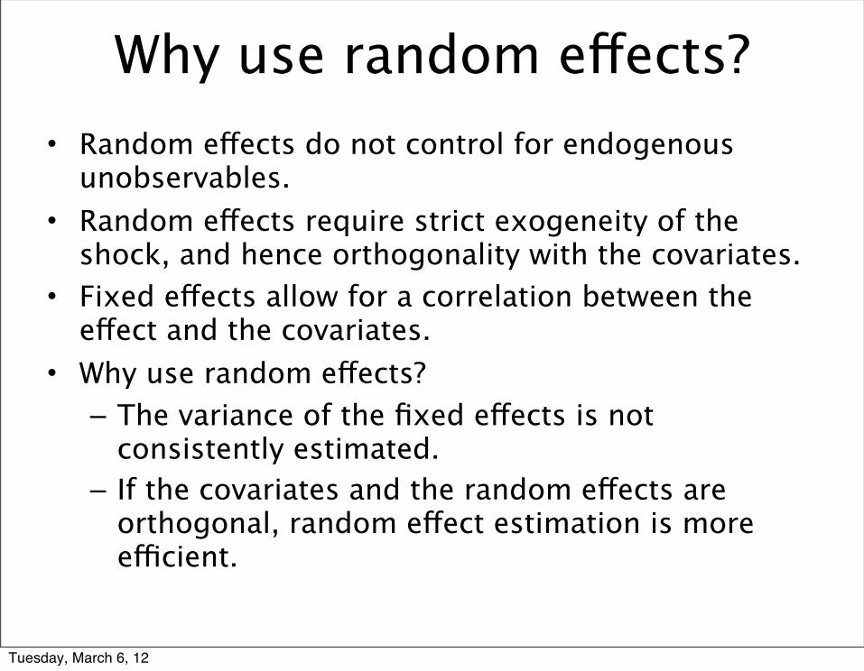
Why use random effects?• Random effects do not control for endogenous

unobservables.• Random effects require strict exogeneity of the

shock, and hence orthogonality with the covariates.• Fixed effects allow for a correlation between the

effect and the covariates.• Why use random effects?– The variance of the fixed effects is not

consistently estimated.– If the covariates and the random effects are

orthogonal, random effect estimation is more efficient.


HAUSMAN TEST


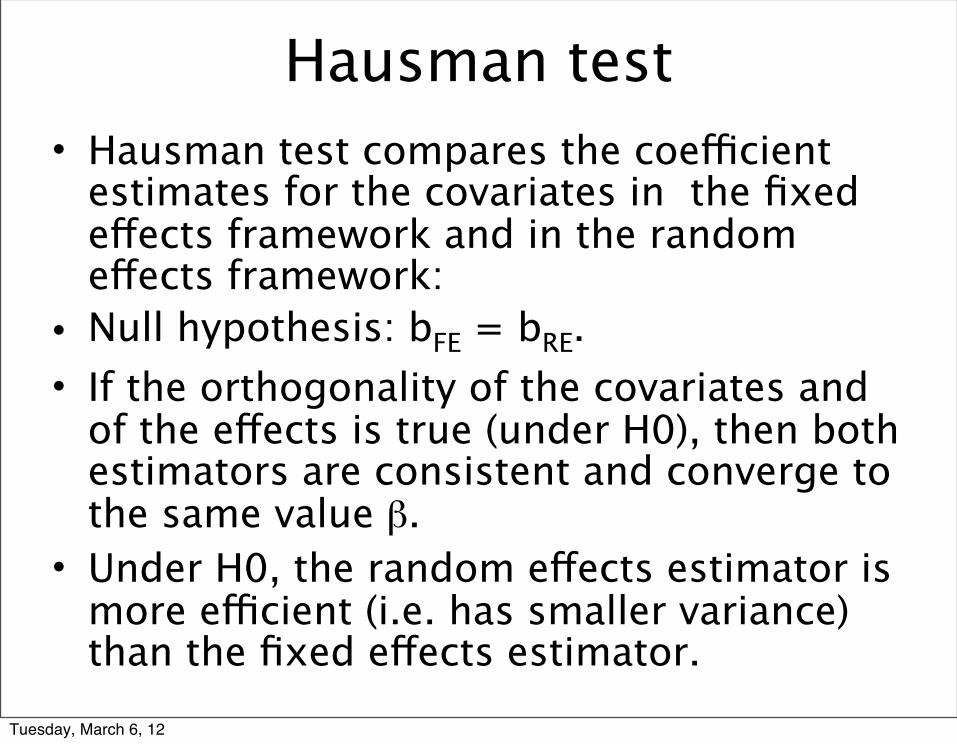
Hausman test• Hausman test compares the coefficient

estimates for the covariates in the fixed effects framework and in the random effects framework:

• Null hypothesis: bFE = bRE.• If the orthogonality of the covariates and

of the effects is true (under H0), then both estimators are consistent and converge to the same value β.

• Under H0, the random effects estimator is more efficient (i.e. has smaller variance) than the fixed effects estimator.


Same logic as for the IV OLS hausman test

• The statistic:

• follows a chi-squared distribution with K-1 degrees of freedom.

36

Greene-50240 book June 18, 2002 15:28


The chi-squared test is based on the Wald criterion:

W = !2[K ! 1] = [b ! !]!"!1[b ! !]. (13-34)

For ", we use the estimated covariance matrices of the slope estimator in the LSDVmodel and the estimated covariance matrix in the random effects model, excluding theconstant term. Under the null hypothesis, W has a limiting chi-squared distribution withK ! 1 degrees of freedom.

Example 13.5 Hausman TestThe Hausman test for the fixed and random effects regressions is based on the parts of the co-efficient vectors and the asymptotic covariance matrices that correspond to the slopes in themodels, that is, ignoring the constant term(s). The coefficient estimates are given in Table 13.2.The two estimated asymptotic covariance matrices are

Est. Var[bF E ] =

!

0.0008934 !0.0003178 !0.001884!0.0003178 0.0002310 !0.0007686!0.001884 !0.0007686 0.04068

"

TABLE 13.2 Random and Fixed Effects Estimates

Parameter Estimates

Specification !1 !2 !3 !4 R2 s2

No effects 9.517 0.88274 0.45398 !1.6275 0.98829 0.015528(0.22924) (0.013255) (0.020304) (0.34530)

Firm effects Fixed effects0.91930 0.41749 !1.0704 0.99743 0.0036125(0.029890) (0.015199) (0.20169)

White(1) (0.019105) (0.013533) (0.21662)White(2) (0.027977) (0.013802) (0.20372)

Fixed effects with autocorrelation " = 0.51620.92975 0.38567 !1.22074 0.0019179(0.033927) (0.0167409) (0.20174) s2/(1 ! "2) =

0.002807

Random effects9.6106 0.90412 0.42390 !1.0646 # 2

u = 0.0119158(0.20277) (0.02462) (0.01375) (0.1993) # 2

$ = 0.00361262

Random effects with autocorrelation " = 0.516210.139 0.91269 0.39123 !1.2074 # 2

u = 0.0268079(0.2587) (0.027783) (0.016294) (0.19852) # 2

$ = 0.0037341

Fixed effectsFirm and timeeffects 12.667 0.81725 0.16861 !0.88281 0.99845 0.0026727

(2.0811) (0.031851) (0.16348) (0.26174)

Random effects9.799 0.84328 0.38760 !0.92943 # 2

u = 0.0142291(0.87910) (0.025839) (0.06845) (0.25721) # 2

$ = 0.0026395# 2

v = 0.0551958


Implementation• Reported by xtreg, re.

• Otherwise use “estimates store” and “hausman”.

• In practice report the Hausman test if using either random effects or fixed effects.

37


TWO WAY FIXED EFFECTS(ABOWD, KRAMARZ, MARGOLIS, 1999)


Two way fixed effects• Estimate the contribution of the

industry, the firm, the CEO to firm performance/the CEO’s wage.

• Example: “Managing with style”, by Marianne Bertrand.


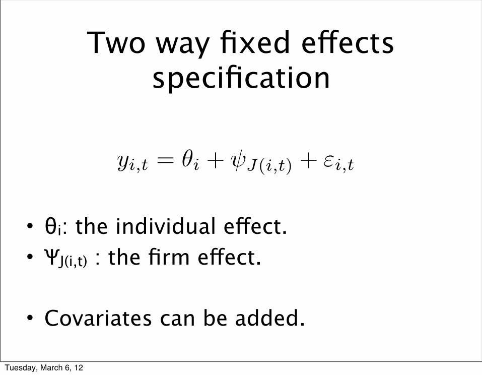
yi,t = ✓i + J(i,t) + "i,t

Two way fixed effects specification

• θi: the individual effect.• ΨJ(i,t) : the firm effect.

• Covariates can be added.


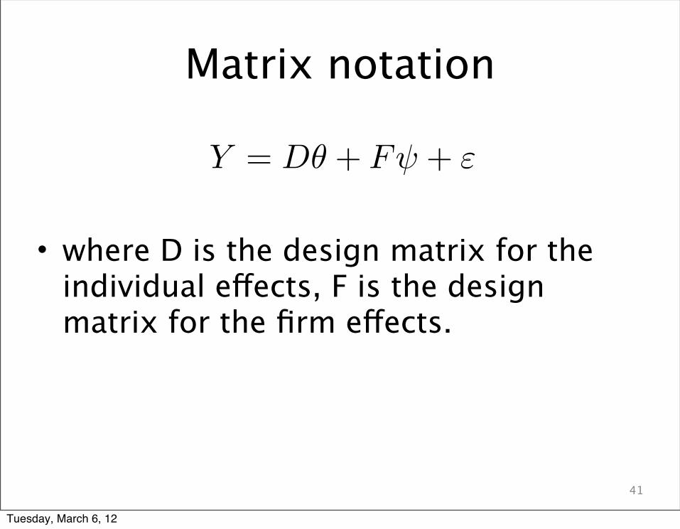
Y = D✓ + F + "

Matrix notation

• where D is the design matrix for the individual effects, F is the design matrix for the firm effects.

41


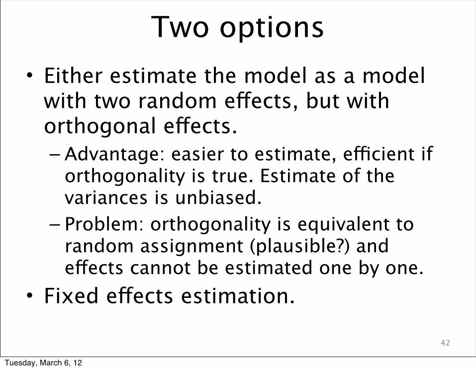
Two options• Either estimate the model as a model

with two random effects, but with orthogonal effects.– Advantage: easier to estimate, efficient if

orthogonality is true. Estimate of the variances is unbiased.

– Problem: orthogonality is equivalent to random assignment (plausible?) and effects cannot be estimated one by one.

• Fixed effects estimation.

42


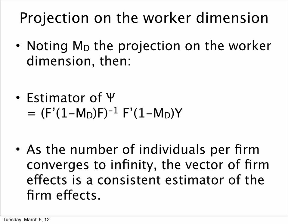
Projection on the worker dimension

• Noting MD the projection on the worker dimension, then:

• Estimator of Ψ = (F’(1-MD)F)-1 F’(1-MD)Y

• As the number of individuals per firm converges to infinity, the vector of firm effects is a consistent estimator of the firm effects.


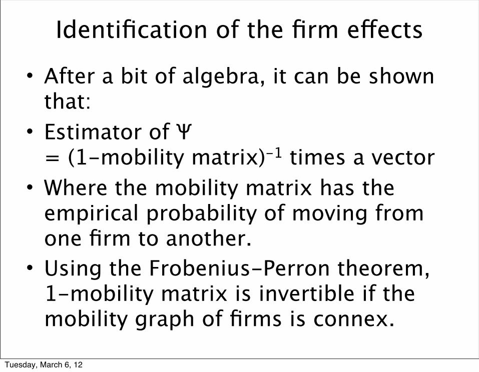
Identification of the firm effects

• After a bit of algebra, it can be shown that:

• Estimator of Ψ = (1-mobility matrix)-1 times a vector

• Where the mobility matrix has the empirical probability of moving from one firm to another.

• Using the Frobenius-Perron theorem, 1-mobility matrix is invertible if the mobility graph of firms is connex.


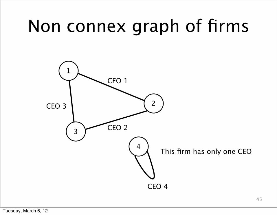
Non connex graph of firms

45

This firm has only one CEO

2

1

3

CEO 1

CEO 2

CEO 3

CEO 4

4


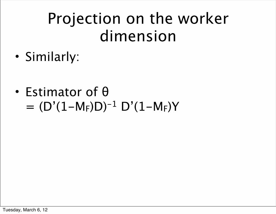
Projection on the worker dimension

• Similarly:

• Estimator of θ = (D’(1-MF)D)-1 D’(1-MF)Y


Identification of the worker effects

• Typically issue is that the number of observations per worker is small and does not converge to infinity.

• Estimate is unbiased but not consistent.

• Variance of the estimate of the individual effect is approximately given by the CLT.


Implementation ofthe identification test

• ssc install a2group

• a2group, individual(ceoid) unit(firmid) generate(group)


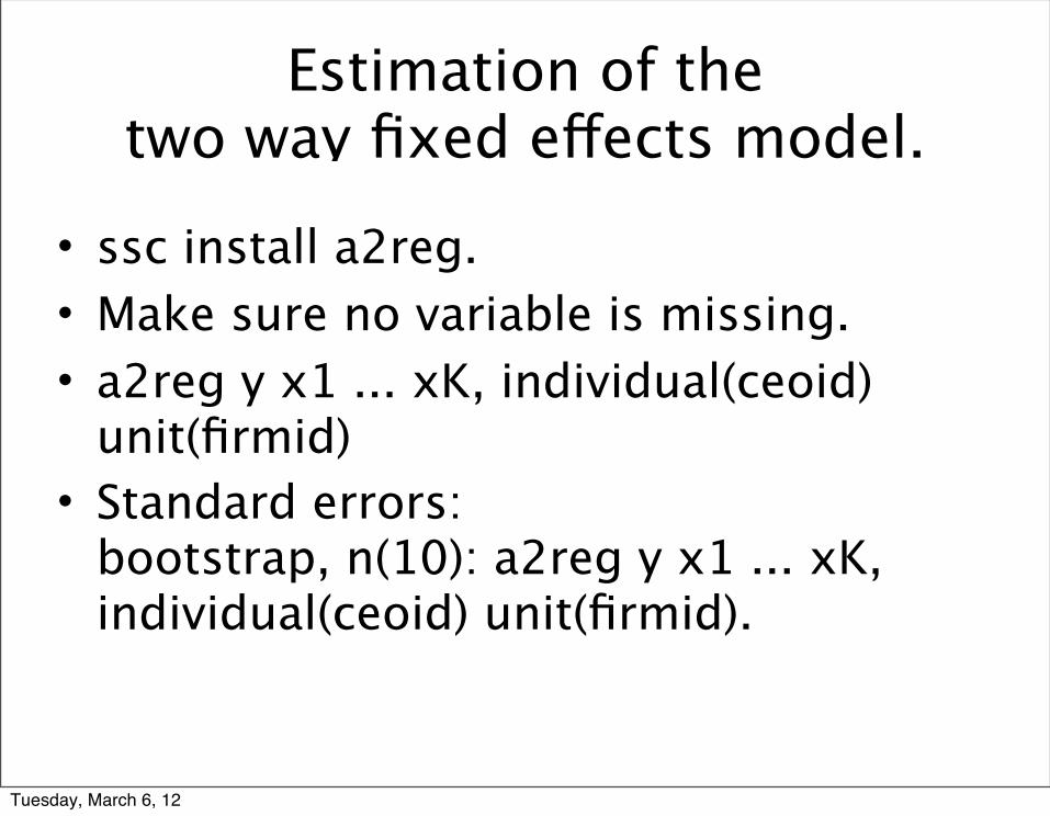
Estimation of the two way fixed effects model.

• ssc install a2reg.• Make sure no variable is missing.• a2reg y x1 ... xK, individual(ceoid)

unit(firmid)• Standard errors:

bootstrap, n(10): a2reg y x1 ... xK, individual(ceoid) unit(firmid).


Estimation of the two way fixed effects model.

• Alternative: OLS with dummies.

• xi: regress y x1 .... xK i.ceoid i.firmid

• Gives standard errors in one step.• But the variance-covariance matrix has

dimension K+# of CEOS+# of firms !


Threats to identification• Correlation between the mobility of a CEO from one

firm to another firm and the unobservable time-varying shocks.

• If good CEOs tend to move to firms that experience an upward trend in their performance, the difference between good and bad CEOs will be overestimated.

• If good CEOs tend to move to firms that experience a downward trend in their performance, the difference between good and bad CEOs will be underestimated.


52

THE

QUARTERLY JOURNALOF ECONOMICS

Vol. CXVIII November 2003 Issue 4

MANAGING WITH STYLE: THE EFFECT OF MANAGERSON FIRM POLICIES*

MARIANNE BERTRAND AND ANTOINETTE SCHOAR

This paper investigates whether and how individual managers affect corpo-rate behavior and performance. We construct a manager-firm matched panel dataset which enables us to track the top managers across different firms over time.We find that manager fixed effects matter for a wide range of corporate decisions.A significant extent of the heterogeneity in investment, financial, and organiza-tional practices of firms can be explained by the presence of manager fixed effects.We identify specific patterns in managerial decision-making that appear to indi-cate general differences in “style” across managers. Moreover, we show thatmanagement style is significantly related to manager fixed effects in performanceand that managers with higher performance fixed effects receive higher compen-sation and are more likely to be found in better governed firms. In a final step, wetie back these findings to observable managerial characteristics. We find thatexecutives from earlier birth cohorts appear on average to be more conservative;on the other hand, managers who hold an MBA degree seem to follow on averagemore aggressive strategies.

I. INTRODUCTION

“In the old days I would have said it was capital, history, the name of thebank. Garbage—it’s about the guy at the top. I am very much a process

* We thank the editors (Lawrence Katz and Edward Glaeser), three anony-mous referees, Kent Daniel, Rebecca Henderson, Steven Kaplan, Kevin J. Mur-phy, Sendhil Mullainathan, Canice Prendergast, David Scharfstein, JerryWarner, Michael Weisbach, seminar participants at Harvard University, theKellogg Graduate School of Management at Northwestern University, the Mas-sachusetts Institute of Technology, the University of Chicago Graduate School ofBusiness, the University of Illinois at Urbana-Champaign, Rochester University,and the Stockholm School of Economics for many helpful comments. We thankKevin J. Murphy and Robert Parrino for generously providing us with their data.Jennifer Fiumara and Michael McDonald provided excellent research assistance.E-mail: [email protected]; [email protected].

© 2003 by the President and Fellows of Harvard College and the Massachusetts Institute ofTechnology.The Quarterly Journal of Economics, November 2003

1169


53

number of acquisitions, but slightly lower cash holdings andleverage levels. It is, however, very similar to the average COM-PUSTAT firm with respect to cash flow, investment levels, divi-dend payouts, R&D, and SG&A.

Table II tabulates the nature of the executive transitions inour sample. We separate three major executive categories: CEOs,CFOs, and “Others.” The majority of the job titles in this “Others”category correspond to operationally important positions: 44 per-cent are subdivision CEOs or Presidents, 16 percent are Execu-tive Vice-Presidents, and 12 percent are COOs; the rest are Vice-Presidents and other more generic titles.

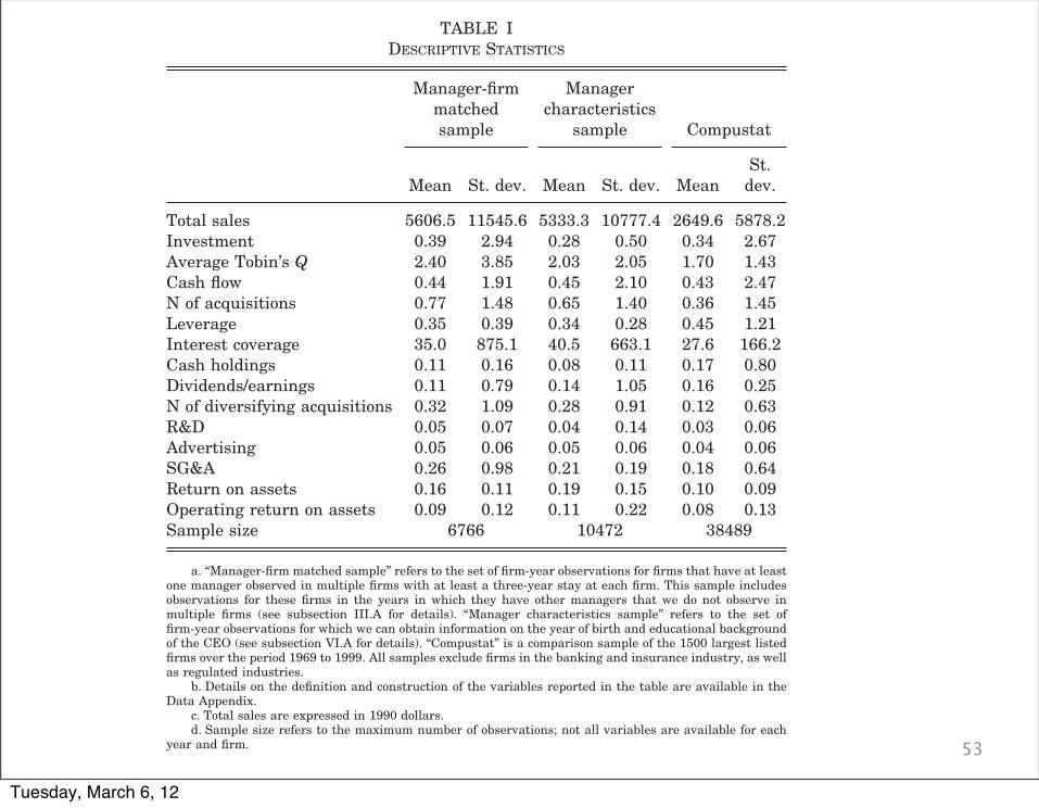
TABLE IDESCRIPTIVE STATISTICS

Manager-firmmatchedsample

Managercharacteristics

sample Compustat

Mean St. dev. Mean St. dev. MeanSt.

dev.

Total sales 5606.5 11545.6 5333.3 10777.4 2649.6 5878.2Investment 0.39 2.94 0.28 0.50 0.34 2.67Average Tobin’s Q 2.40 3.85 2.03 2.05 1.70 1.43Cash flow 0.44 1.91 0.45 2.10 0.43 2.47N of acquisitions 0.77 1.48 0.65 1.40 0.36 1.45Leverage 0.35 0.39 0.34 0.28 0.45 1.21Interest coverage 35.0 875.1 40.5 663.1 27.6 166.2Cash holdings 0.11 0.16 0.08 0.11 0.17 0.80Dividends/earnings 0.11 0.79 0.14 1.05 0.16 0.25N of diversifying acquisitions 0.32 1.09 0.28 0.91 0.12 0.63R&D 0.05 0.07 0.04 0.14 0.03 0.06Advertising 0.05 0.06 0.05 0.06 0.04 0.06SG&A 0.26 0.98 0.21 0.19 0.18 0.64Return on assets 0.16 0.11 0.19 0.15 0.10 0.09Operating return on assets 0.09 0.12 0.11 0.22 0.08 0.13Sample size 6766 10472 38489

a. “Manager-firm matched sample” refers to the set of firm-year observations for firms that have at leastone manager observed in multiple firms with at least a three-year stay at each firm. This sample includesobservations for these firms in the years in which they have other managers that we do not observe inmultiple firms (see subsection III.A for details). “Manager characteristics sample” refers to the set offirm-year observations for which we can obtain information on the year of birth and educational backgroundof the CEO (see subsection VI.A for details). “Compustat” is a comparison sample of the 1500 largest listedfirms over the period 1969 to 1999. All samples exclude firms in the banking and insurance industry, as wellas regulated industries.

b. Details on the definition and construction of the variables reported in the table are available in theData Appendix.

c. Total sales are expressed in 1990 dollars.d. Sample size refers to the maximum number of observations; not all variables are available for each

year and firm.

1177MANAGING WITH STYLE


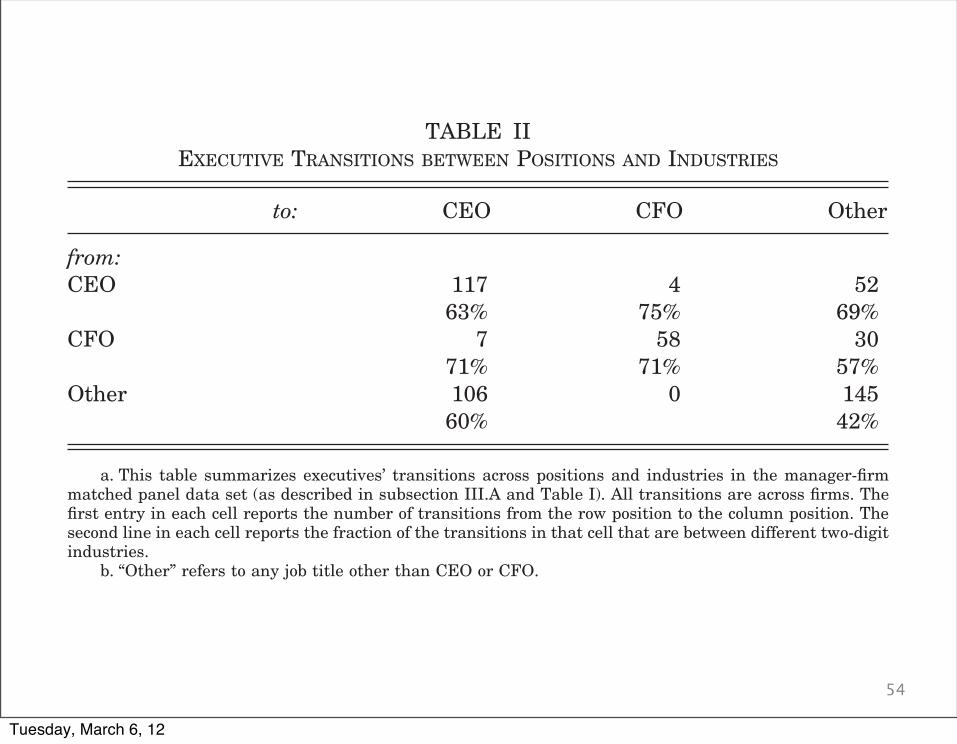
54Of the set of about 500 managers identified in our sample,

117 are individuals who move from a CEO position in one firm toa CEO position in another firm; 4 are CEOs who move to CFOpositions; and 52 are CEOs who move to other top positions.Among the set of executives starting as CFOs, we observe 7becoming CEOs, 58 moving to another CFO position, and 30moving to other top positions. Finally, among the 251 managerswho start in another top position, 106 become CEOs, and 145move to another non-CEO, non-CFO position. Within this lattergroup we found that more than 40 percent of the transitions aremoves from a position of subdivision CEO or subdivision presi-dent in one firm to a similar position in another firm.

In the second row of each cell in Table II, we report thefraction of moves that are between firms in different two-digitindustries.15 It is interesting to note that a large fraction of theexecutive moves in our sample are between industries. For exam-ple, 63 percent of the CEO to CEO moves are across differenttwo-digit industries, as are 71 percent of the CFO to CFO moves.A relatively lower fraction of the moves from other top positionsto other top positions (42 percent) are across industries. Thesepatterns seem intuitive if ones believes that CEOs and CFOsneed relatively less industry and firm-specific knowledge andinstead rely more on general management skills.16

15. The industry classification is based on the primary SIC code of each firm,as reported in COMPUSTAT.

16. See, for example, Fligstein [1990] for a discussion of this argument.

TABLE IIEXECUTIVE TRANSITIONS BETWEEN POSITIONS AND INDUSTRIES

to: CEO CFO Other

from:CEO 117 4 52

63% 75% 69%CFO 7 58 30

71% 71% 57%Other 106 0 145

60% 42%

a. This table summarizes executives’ transitions across positions and industries in the manager-firmmatched panel data set (as described in subsection III.A and Table I). All transitions are across firms. Thefirst entry in each cell reports the number of transitions from the row position to the column position. Thesecond line in each cell reports the fraction of the transitions in that cell that are between different two-digitindustries.

b. “Other” refers to any job title other than CEO or CFO.

1178 QUARTERLY JOURNAL OF ECONOMICS


55

IV. IS THERE HETEROGENEITY IN EXECUTIVE PRACTICES?

IV.A. Empirical Methodology

The nature of our identification strategy can be most easilyexplained with an example. Consider the dividend payout ratio asthe corporate policy of interest. From a benchmark specificationwe derive residual dividend payouts at the firm-year level aftercontrolling for any average differences across firms and years aswell as for any firm-year specific shock, such as an earningsshock, that might affect the dividend payout of a firm. We thenask how much of the variance in these residual dividend payoutscan be attributed to manager-specific effects.

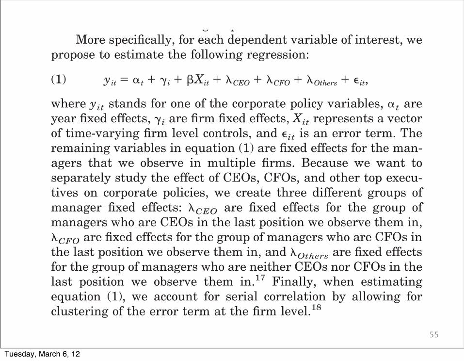
More specifically, for each dependent variable of interest, wepropose to estimate the following regression:

(1) yit ! !t " "i " #Xit " $CEO " $CFO " $Others " %it,

where yit stands for one of the corporate policy variables, !t areyear fixed effects, "i are firm fixed effects, Xit represents a vectorof time-varying firm level controls, and %it is an error term. Theremaining variables in equation (1) are fixed effects for the man-agers that we observe in multiple firms. Because we want toseparately study the effect of CEOs, CFOs, and other top execu-tives on corporate policies, we create three different groups ofmanager fixed effects: $CEO are fixed effects for the group ofmanagers who are CEOs in the last position we observe them in,$CFO are fixed effects for the group of managers who are CFOs inthe last position we observe them in, and $Others are fixed effectsfor the group of managers who are neither CEOs nor CFOs in thelast position we observe them in.17 Finally, when estimatingequation (1), we account for serial correlation by allowing forclustering of the error term at the firm level.18

It is evident from equation (1) that the estimation of themanager fixed effects is not possible for managers who neverleave a given company during our sample period. Consider, forexample, a specific manager who never switches companies andadvances only through internal promotions, maybe moving from

17. We also repeated all of the analyses below after separating CEO to CEOmoves, CEO to CFO moves, etc. The results were qualitatively similar to the moreaggregated results reported in the paper.

18. In subsection IV.C we propose two alternative estimation methods to dealwith serial correlation issues and better address possible issues regarding thepersistence of the manager fixed effects.



56

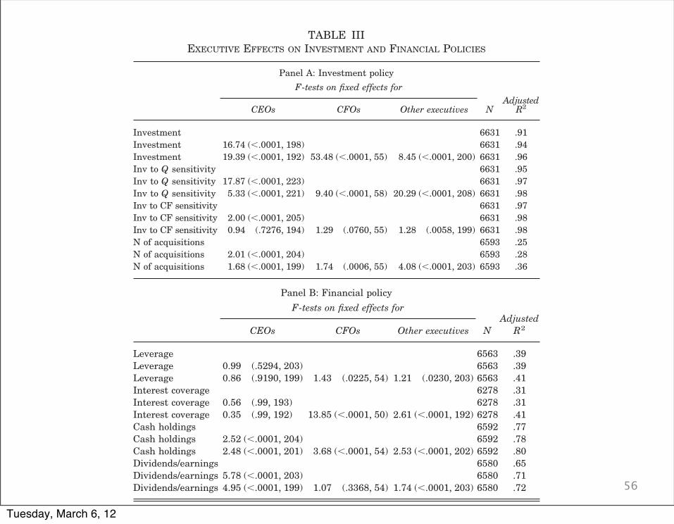
TABLE IIIEXECUTIVE EFFECTS ON INVESTMENT AND FINANCIAL POLICIES

Panel A: Investment policyF-tests on fixed effects for

NAdjusted

R2CEOs CFOs Other executives

Investment 6631 .91Investment 16.74 (!.0001, 198) 6631 .94Investment 19.39 (!.0001, 192) 53.48 (!.0001, 55) 8.45 (!.0001, 200) 6631 .96Inv to Q sensitivity 6631 .95Inv to Q sensitivity 17.87 (!.0001, 223) 6631 .97Inv to Q sensitivity 5.33 (!.0001, 221) 9.40 (!.0001, 58) 20.29 (!.0001, 208) 6631 .98Inv to CF sensitivity 6631 .97Inv to CF sensitivity 2.00 (!.0001, 205) 6631 .98Inv to CF sensitivity 0.94 (.7276, 194) 1.29 (.0760, 55) 1.28 (.0058, 199) 6631 .98N of acquisitions 6593 .25N of acquisitions 2.01 (!.0001, 204) 6593 .28N of acquisitions 1.68 (!.0001, 199) 1.74 (.0006, 55) 4.08 (!.0001, 203) 6593 .36

Panel B: Financial policyF-tests on fixed effects for

NAdjusted

R2CEOs CFOs Other executives

Leverage 6563 .39Leverage 0.99 (.5294, 203) 6563 .39Leverage 0.86 (.9190, 199) 1.43 (.0225, 54) 1.21 (.0230, 203) 6563 .41Interest coverage 6278 .31Interest coverage 0.56 (.99, 193) 6278 .31Interest coverage 0.35 (.99, 192) 13.85 (!.0001, 50) 2.61 (!.0001, 192) 6278 .41Cash holdings 6592 .77Cash holdings 2.52 (!.0001, 204) 6592 .78Cash holdings 2.48 (!.0001, 201) 3.68 (!.0001, 54) 2.53 (!.0001, 202) 6592 .80Dividends/earnings 6580 .65Dividends/earnings 5.78 (!.0001, 203) 6580 .71Dividends/earnings 4.95 (!.0001, 199) 1.07 (.3368, 54) 1.74 (!.0001, 203) 6580 .72

a. Sample is the manager-firm matched panel data set as described in subsection III.A and Table I.Details on the definition and construction of the variables reported in the table are available in the DataAppendix.

b. Reported in the table are the results from fixed effects panel regressions, where standard errors areclustered at the firm level. For each dependent variable (as reported in column 1), the fixed effects includedare row 1: firm and year fixed effects; row 2: firm, year, and CEO fixed effects; row 3: firm, year, CEO, CFO,and other executives fixed effects. Included in the “Investment to Q” and “Investment to cash flow” regres-sions are interactions of these fixed effects with lagged Tobin’s Q and cash flow, respectively. Also the“Investment,” “Investment to Q,” and “Investment to cash flow” regressions include lagged logarithm of totalassets, lagged Tobin’s Q, and cash flow. The “Number of Acquisitions” regressions include lagged logarithmof total assets and return on assets. Each regression in Panel B contains return on assets, cash flow, and thelagged logarithm of total assets.

c. Reported are the F-tests for the joint significance of the CEO fixed effects (column 2), CFO fixed effects(column 3), and other executives fixed effects (column 4). For each F-test we report the value of the F-statistic,the p-value, and the number of constraints. For the “Investment to Q” and “Investment to Cash Flow”regressions, the F-tests are for the joint significance of the interactions between the manager fixed effects andTobin’s Q and cash flow, respectively. Column 5 reports the number of observations, and column 6 theadjusted R2s for each regression.



57

quartile of the distribution increases the rate of return on assetsby about 3 percent. In contrast, a manager in the bottom quartilereduces the rate of return on assets by about 3 percent.

Also, the median manager fixed effects for most of the corpo-rate variables are not different from zero. This is interesting asone might have expected that the nature of the sample construc-tion and the focus on outside hires might have led us to select adifferent type of managers. This seems to indicate that this pos-sible selection issue is not an important factor in our analysis.

IV.E. Management Styles

The previous section documents a wide degree of heteroge-neity in the way managers conduct their businesses. We nowwant to go a step further and investigate whether there areoverarching patterns in managerial decision-making. For exam-ple, do some managers favor internal growth strategies whileothers rely more on external growth, ceteris paribus? Or can weobserve that some managers overall are financially more aggres-sive than others?

TABLE VISIZE DISTRIBUTION OF MANAGER FIXED EFFECTS

MedianStandarddeviation

25thpercentile

75thpercentile

Investment 0.00 2.80 !0.09 0.11Inv to Q sensitivity !0.02 0.66 !0.16 0.12Inv to CF sensitivity 0.04 1.01 !0.17 0.28N of acquisitions !0.04 1.50 !0.54 0.41Leverage 0.01 0.22 !0.05 0.09Interest coverage 0.00 860.0 !56.0 51.7Cash holdings 0.00 0.06 !0.03 0.02Dividends/earnings !0.01 0.59 !0.13 0.11N of diversifying acquis. !0.04 1.05 !0.28 0.21R&D 0.00 0.04 !0.10 0.02SG&A 0.00 0.66 !0.09 0.09Advertising 0.00 0.04 !0.01 0.01Return on assets 0.00 0.07 !0.03 0.03Operating return on assets 0.00 0.08 !0.02 0.03

a. The fixed effects used in this table are retrieved from the regressions reported in Tables III and IV (row3).

b. Column 1 reports the median fixed effect for each policy variable. Column 2 reports the standarddeviation of the fixed effects. Columns 3 and 4 report the fixed effects at the twenty-fifth percentile andseventy-fifth percentile of the distribution, respectively.

c. Each fixed effect is weighted by the inverse of its standard error to account for estimation error.



58

To answer these questions, we analyze the correlation struc-ture between the manager specific fixed effects which we retrievefrom the set of regressions above. We form a data set that, foreach manager, contains the estimated fixed effects for the variouscorporate variables. More precisely, the different variables in thisnew data set are the manager fixed effects estimated in Tables IIIand IV for the specification that includes all groups of managers(row 3).

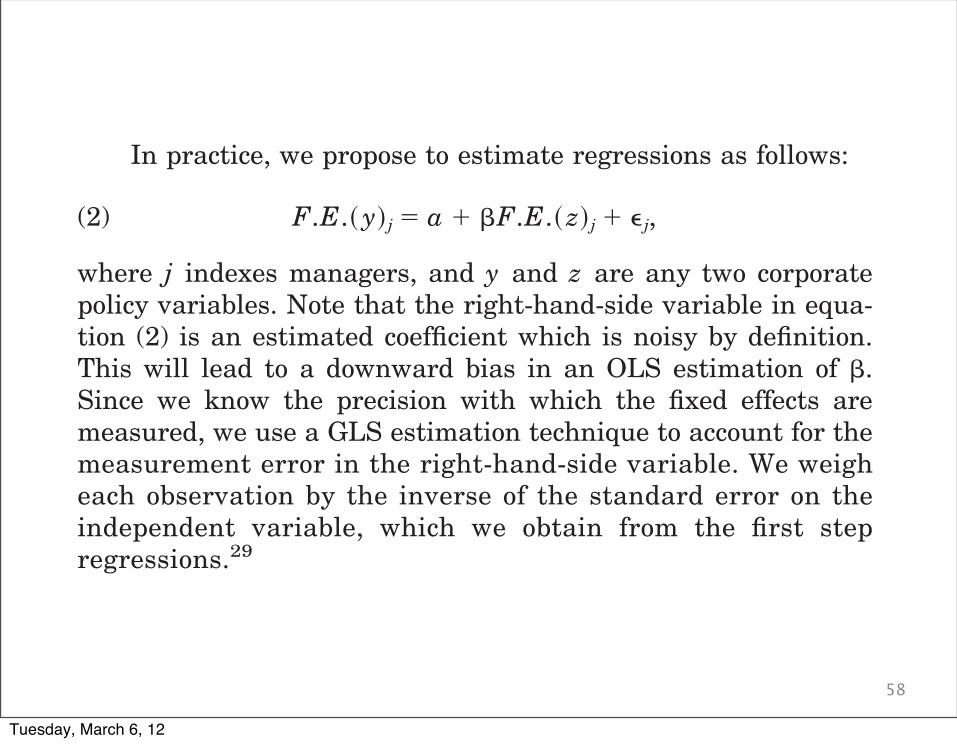
In practice, we propose to estimate regressions as follows:

(2) F.E.! y"j ! a " #F.E.! z"j " $j,

where j indexes managers, and y and z are any two corporatepolicy variables. Note that the right-hand-side variable in equa-tion (2) is an estimated coefficient which is noisy by definition.This will lead to a downward bias in an OLS estimation of #.Since we know the precision with which the fixed effects aremeasured, we use a GLS estimation technique to account for themeasurement error in the right-hand-side variable. We weigheach observation by the inverse of the standard error on theindependent variable, which we obtain from the first stepregressions.29

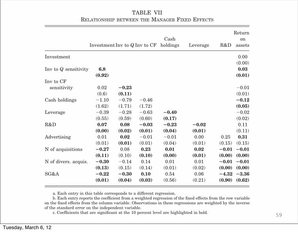
The results of this exercise are reported in Table VII. Eachelement in this table corresponds to a different regression. Theaverage R2 for these regressions is about 10 percent; the maxi-mum R2 is about 33 percent, while the minimum R2 is about 0.03percent. A few interesting patterns seem to emerge from thistable. First, managers seem to differ in their approach towardexternal versus internal growth. We see from the last two rows ofcolumn 1 that there is a strong negative correlation betweencapital expenditures, which can be interpreted as internal invest-ments, and external growth through acquisitions and diversifica-tion. In a similar vein, managers who follow expansion strategiesthrough external acquisitions and diversification engage in lessR&D expenditures. Row 7 of Table VII shows that the coefficients

29. We also repeated this analysis using a different technique to account formeasurement error in the estimated fixed effect. For each set of fixed effects weformed averages of the observations by deciles (ranking observations by size), andthen regressed the transformed set of fixed effects on each other in the above-described manner. This produces qualitatively similar results. Finally, we alsoconducted a factor analysis for the full set of fixed effects. We were able todistinguish three different eigenvectors. The factor loadings seem to support theview that financial aggressiveness and internal versus external growth are twoimportant dimensions of style.



59

from a regression of R&D on either of these variables are !0.01with standard errors of 0.002. Moreover, capital expenditures andR&D expenditures are significantly positively correlated.

Another interesting finding is that managers who are moreinvestment-Q sensitive also appear to be less investment-cashsensitive. The coefficient on " in a regression of the investment toQ fixed effects on the investment to cash flow fixed effects (column2 and row 3 of Table VII) is !0.23 with a standard error of 0.11.This suggests that managers may follow one of two strategies:either use the firm’s market valuation or use the cash flow gen-erated by operations as a benchmark for their investment deci-sions. This result is interesting in light of the current debate onthe investment to cash flow sensitivity in firms. So far, mostresearch has analyzed differences in investment behavior acrossfirms along a financial constraint dimension. Our findings sug-

TABLE VIIRELATIONSHIP BETWEEN THE MANAGER FIXED EFFECTS

Investment Inv to Q Inv to CFCash

holdings Leverage R&D

Returnon

assets

Investment 0.00(0.00)

Inv to Q sensitivity 6.8 0.03(0.92) (0.01)

Inv to CFsensitivity 0.02 !0.23 !0.01

(0.6) (0.11) (0.01)Cash holdings !1.10 !0.79 !0.46 !0.12

(1.62) (1.71) (1.72) (0.05)Leverage !0.39 !0.28 !0.63 !0.40 !0.02

(0.55) (0.59) (0.60) (0.17) (0.02)R&D 0.07 0.08 !0.03 !0.23 !0.02 0.11

(0.00) (0.02) (0.01) (0.04) (0.01) (0.11)Advertising 0.01 0.02 !0.01 !0.01 0.00 0.25 0.31

(0.01) (0.01) (0.01) (0.04) (0.01) (0.15) (0.15)N of acquisitions !0.27 0.08 0.23 0.01 0.02 !0.01 !0.01

(0.11) (0.10) (0.10) (0.00) (0.01) (0.00) (0.00)N of divers. acquis. !0.30 !0.14 0.14 0.01 0.01 !0.01 !0.01

(0.13) (0.15) (0.14) (0.01) (0.02) (0.00) (0.00)SG&A !0.22 !0.30 0.10 0.54 0.06 !4.32 !3.36

(0.01) (0.04) (0.03) (0.56) (0.21) (0.90) (0.62)

a. Each entry in this table corresponds to a different regression.b. Each entry reports the coefficient from a weighted regression of the fixed effects from the row variable

on the fixed effects from the column variable. Observations in these regressions are weighted by the inverseof the standard error on the independent variable.

c. Coefficients that are significant at the 10 percent level are highlighted in bold.



Panel Data Analysis - Amine Ouazad · Balanced panel data • Balanced panel data: ... • Checking...

Documents

Transcript of Panel Data Analysis - Amine Ouazad · Balanced panel data • Balanced panel data: ... • Checking...