ASSOCIATION: CONTINGENCY, CORRELATION, AND REGRESSION Chapter 3.
35
ASSOCIATION: CONTINGENCY, CORRELATION, AND REGRESSION Chapter 3
-
Upload
claude-ferguson -
Category
Documents
-
view
237 -
download
6
Transcript of ASSOCIATION: CONTINGENCY, CORRELATION, AND REGRESSION Chapter 3.
ASSOCIATION: CONTINGENCY, CORRELATION, AND REGRESSION
Chapter 3


3.1 The Association between Two Categorical Variables

Response and Explanatory Variables
Response variable (dependent, y) outcome variable
Explanatory variable (independent, x) defines groups
Response/Explanatory1. Grade on
test/Amount of study time
2. Yield of corn/Amount of rainfall

Association
Association – When a value for one variable is more likely with certain values of the other variable
Data analysis with two variables 1. Tell whether there is an association and 2. Describe that association

Contingency Table
Displays two categorical variables
The rows list the categories of one variable; the columns list the other
Entries in the table are frequencies
www1.pictures.fp.zimbio.com

Contingency Table
What is the response (outcome) variable? Explanatory?
What proportion of organic foods contain pesticides?Conventionally grown?
What proportion of all sampled foods contain pesticides?

Proportions & Conditional Proportions

Side by side bar charts show conditional proportions and allow for easy comparison
Proportions & Conditional Proportions
www.vitalchoice.com

If no association, then proportions would be the same
Proportions & Conditional Proportions
Since there is association, then proportions are different

3.2 The Association between Two Quantitative Variables

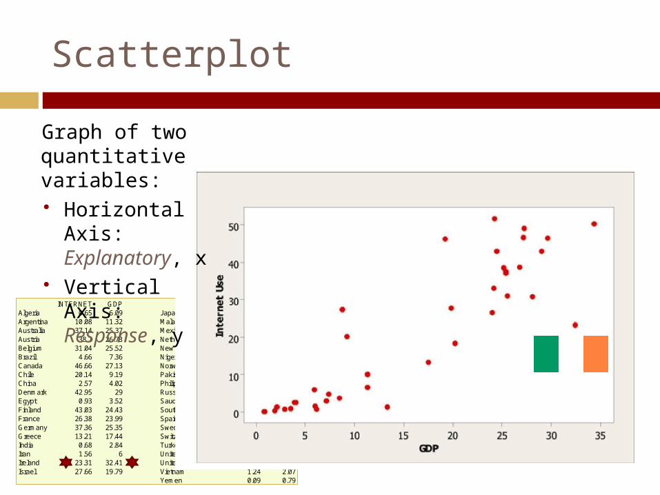
Internet Usage & GDP Data Set
INTERNET GDP INTERNET GDPAlgeria 0.65 6.09 J apan 38.42 25.13Argentina 10.08 11.32 Malaysia 27.31 8.75Australia 37.14 25.37 Mexico 3.62 8.43Austria 38.7 26.73 Netherlands 49.05 27.19Belgium 31.04 25.52 New Zealand 46.12 19.16Brazil 4.66 7.36 Nigeria 0.1 0.85Canada 46.66 27.13 Norway 46.38 29.62Chile 20.14 9.19 Pakistan 0.34 1.89China 2.57 4.02 Philippines 2.56 3.84Denmark 42.95 29 Russia 2.93 7.1Egypt 0.93 3.52 Saudi Arabia 1.34 13.33Finland 43.03 24.43 South Africa 6.49 11.29France 26.38 23.99 Spain 18.27 20.15Germany 37.36 25.35 Sweden 51.63 24.18Greece 13.21 17.44 Switzerland 30.7 28.1India 0.68 2.84 Turkey 6.04 5.89Iran 1.56 6 United Kingdom 32.96 24.16Ireland 23.31 32.41 United States 50.15 34.32Israel 27.66 19.79 Vietnam 1.24 2.07
Yemen 0.09 0.79
www.knitwareblog.com
INTERNET GDP INTERNET GDPAlgeria 0.65 6.09 J apan 38.42 25.13Argentina 10.08 11.32 Malaysia 27.31 8.75Australia 37.14 25.37 Mexico 3.62 8.43Austria 38.7 26.73 Netherlands 49.05 27.19Belgium 31.04 25.52 New Zealand 46.12 19.16Brazil 4.66 7.36 Nigeria 0.1 0.85Canada 46.66 27.13 Norway 46.38 29.62Chile 20.14 9.19 Pakistan 0.34 1.89China 2.57 4.02 Philippines 2.56 3.84Denmark 42.95 29 Russia 2.93 7.1Egypt 0.93 3.52 Saudi Arabia 1.34 13.33Finland 43.03 24.43 South Africa 6.49 11.29France 26.38 23.99 Spain 18.27 20.15Germany 37.36 25.35 Sweden 51.63 24.18Greece 13.21 17.44 Switzerland 30.7 28.1India 0.68 2.84 Turkey 6.04 5.89Iran 1.56 6 United Kingdom 32.96 24.16Ireland 23.31 32.41 United States 50.15 34.32Israel 27.66 19.79 Vietnam 1.24 2.07
Yemen 0.09 0.79
Scatterplot
Graph of two quantitative variables: Horizontal Axis:
Explanatory, x Vertical Axis:
Response, y

Interpreting Scatterplots
The overall pattern includes trend, direction, and strength of the relationship Trend: linear, curved,
clusters, no pattern Direction: positive,
negative, no direction Strength: how closely
the points fit the trend Also look for outliers
from the overall trend

Used-car Dealership
What association would we expect between the age of the car and mileage?
a) Positiveb) Negativec) No association

Linear Correlation, r
Measures the strength and direction of the linear association between x and y

Correlation coefficient: Measuring Strength & Direction of a Linear Relationship
Positive r => positive associationNegative r => negative associationr close to +1 or -1 indicates strong linear associationr close to 0 indicates weak association

3.3 Can We Predict the Outcome of a Variable?

Regression Line
Predicts y, given x:
The y-intercept and slope are a and b
Only an estimate – actual data vary
Describes relationship between x and estimated means of y
bxay ˆ
farm4.static.flickr.com

Residuals
Prediction errors: vertical distance between data point and regression line
Large residual indicates unusual observation
Each residual is:
Sum of residuals is always zero
ˆy y
www.chem.utoronto.ca
Goal: Minimize distance from data to regression line

msenux.redwoods.edu
Least Squares Method
Residual sum of squares:
Least squares regression line minimizes vertical distance between points and their predictions
2 2ˆ( ) ( )residuals y y

Regression Analysis
Identify response and explanatory variables Response
variable is y Explanatory
variable is x

Anthropologists Predict Height Using Remains?
Regression Equation:
is predicted height and x is the length of a femur, thighbone (cm)
Predict height for femur length of 50 cm
xy 4.24.61ˆ y
www.geektoysgamesandgadgets.comBones

Interpreting the y-Intercept and slope
y-intercept: y-value when x = 0
Helps plot line Slope: change in y
for 1 unit increase in x
1 cm increase in femur length means 2.4 cm increase in predicted height
xy 4.24.61ˆ

Slope Values: Positive, Negative, Zero

Slope and Correlation
Correlation, r:
Describes strength
No units Same if x and y
are swapped
Slope, b:
Doesn’t tell strength
Has units Inverts if x and y
are swapped

Proportional reduction in error, r2
Variation in y-values explained by relationship of y to x
A correlation, r, of .9 means
81% of variation in y is explained by x
%8181.9. 22 r
Squared Correlation, r2

3.4 What Are Some Cautions in Analyzing Associations?

Extrapolation
Extrapolation: Predicting y for x-values outside range of data Riskier the
farther from the range of x
No guarantee trend holds
Neil Weiss, Elementary Statistics, 7th Edition

Outliers and Influential Points
Regression outlier lies far away from rest of data
Influential if both:
1. Low or high, compared to rest of data
2. Regression outlier
www2.selu.edu

Correlation Does Not Imply Causation
Strong correlation between x and y means
Strong linear association between the variables
Does not mean x causes y
Ex. 95.6% of cancer patients have eaten pickles, so do pickles cause cancer?

Lurking Variables & Confounding
1. Ice cream sales & drowning => temperature2. Reading level & shoe size => age
Confounding – two explanatory variables both associated with response variable and each other
Lurking variables – not measured in study but may confound

Simpson’s Paradox Example
Probability of Death of Smoker = 139/582 = 24%
Probability of Death of Nonsmoker = 230/732 = 31%
Simpson’s Paradox:
Association between two variables reverses after third is included

Break out Data by Age
Simpson’s Paradox Example

Associations look quite different after adjusting for third variable
Simpson’s Paradox Example