Assignment 5

March 6, 2019

1 CSE 252B: Computer Vision II, Winter 2019 – Assignment 5

1.0.1 Instructor: Ben Ochoa

1.0.2 Due: Wednesday, March 20, 2019, 11:59 PM

1.1 Instructions

• Review the academic integrity and collaboration policies on the course website.• This assignment must be completed individually.• This assignment contains both math and programming problems.• All solutions must be written in this notebook• Math problems must be done in Markdown/LATEX. Remember to show work and describe

your solution.• Programming aspects of this assignment must be completed using Python in this notebook.• Your code should be well written with sufficient comments to understand, but there is no

need to write extra markdown to describe your solution if it is not explictly asked for.• This notebook contains skeleton code, which should not be modified (This is important for

standardization to facilate effeciant grading).• You may use python packages for basic linear algebra, but you may not use packages that

directly solve the problem. Ask the instructor if in doubt.• You must submit this notebook exported as a pdf. You must also submit this notebook as an

.ipynb file.• Your code and results should remain inline in the pdf (Do not move your code to an ap-

pendix).• You must submit both files (.pdf and .ipynb) on Gradescope. You must mark each problem

on Gradescope in the pdf.• It is highly recommended that you begin working on this assignment early.

1.2 Problem 1 (Math): Point on Line Closest to the Origin (5 points)

Given a line l = (a, b, c)⊤, show that the point on l that is closest to the origin is the pointx = (−ac,−bc, a2 + b2)⊤ (Hint: this calculation is needed in the two-view optimal triangulationmethod used below).

"""your solution here"""

1

1.3 Problem 2 (Programming): Feature Detection (20 points)

Download input data from the course website. The file IMG_5030.JPG contains image 1 and thefile IMG_5031.JPG contains image 2.

For each input image, calculate an image where each pixel value is the minor eigenvalue of thegradient matrix

N =

∑w

I2x ∑

wIx Iy

∑w

Ix Iy ∑w

I2y

where w is the window about the pixel, and Ix and Iy are the gradient images in the x and y

direction, respectively. Calculate the gradient images using the fivepoint central difference oper-ator. Set resulting values that are below a specified threshold value to zero (hint: calculating themean instead of the sum in N allows for adjusting the size of the window without changing thethreshold value). Apply an operation that suppresses (sets to 0) local (i.e., about a window) non-maximum pixel values in the minor eigenvalue image. Vary these parameters such that around1350–1400 features are detected in each image. For resulting nonzero pixel values, determine thesubpixel feature coordinate using the Forstner corner point operator.

Report your final values for:

• the size of the feature detection window (i.e. the size of the window used to calculate theelements in the gradient matrix N)

• the minor eigenvalue threshold value• the size of the local nonmaximum suppression window• the resulting number of features detected (i.e. corners) in each image.

Display figures for:

• original images with detected features, where the detected features are indicated by a squarewindow (the size of the detection window) about the features

In [28]: %matplotlib inlineimport numpy as npimport matplotlib.pyplot as pltimport matplotlib.patches as patchesfrom scipy.signal import convolve2d as conv2d

def ImageGradient(I, w, t):# inputs:# I is the input image (may be mxn for Grayscale or mxnx3 for RGB)# w is the size of the window used to compute the gradient matrix N# t is the minor eigenvalue threshold## outputs:# N is the 2x2xmxn gradient matrix# b in the 2x1xmxn vector used in the Forstner corner detector# J0 is the mxn minor eigenvalue image of N before thresholding# J1 is the mxn minor eigenvalue image of N after thresholding

2

m,n = I.shape[:2]N = np.zeros((2,2,m,n))b = np.zeros((2,1,m,n))J0 = np.zeros((m,n))J1 = np.zeros((m,n))

"""your code here"""

return N, b, J0, J1

def NMS(J, w_nms):# Apply nonmaximum supression to J using window w# For any window in J, the result should only contain 1 nonzero value# In the case of multiple identical maxima in the same window,# the tie may be broken arbitrarily## inputs:# J is the minor eigenvalue image input image after thresholding# w_nms is the size of the local nonmaximum suppression window## outputs:# J2 is the mxn resulting image after applying nonmaximum suppression#

J2 = J.copy()"""your code here"""

return J2

def ForstnerCornerDetector(J, N, b):# Gather the coordinates of the nonzero pixels in J# Then compute the sub pixel location of each point using the Forstner operator## inputs:# J is the NMS image# N is the 2x2xmxn gradient matrix# b is the 2x1xmxn vector computed in the image_gradient function## outputs:# C is the number of corners detected in each image# pts is the 2xC list of coordinates of subpixel accurate corners

3

# found using the Forstner corner detector

"""your code here"""

pts = np.vstack((np.random.randint(0,1024,(1,625)), np.random.randint(0,768,(1,625))))C = len(pts[0])return C, pts

# feature detectiondef RunFeatureDetection(I, w, t, w_nms):

N, b, J0, J1 = ImageGradient(I, w, t)J2 = NMS(J1, w_nms)C, pts = ForstnerCornerDetector(J2, N, b)return C, pts, J0, J1, J2

In [69]: from PIL import Imageimport time

# input imagesI1 = np.array(Image.open('IMG_5030.JPG'), dtype='float')/255.I2 = np.array(Image.open('IMG_5031.JPG'), dtype='float')/255.

# parameters to tunew = 15t = 1w_nms = 1

tic = time.time()

# run feature detection algorithm on input imagesC1, pts1, J1_0, J1_1, J1_2 = RunFeatureDetection(I1, w, t, w_nms)C2, pts2, J2_0, J2_1, J2_2 = RunFeatureDetection(I2, w, t, w_nms)toc = time.time() - tic

print('took %f secs'%toc)

# display resultsplt.figure(figsize=(14,24))

# show corners on original imagesax = plt.subplot(1,2,1)plt.imshow(I1)for i in range(C1): # draw rectangles of size w around corners

x,y = pts1[:,i]ax.add_patch(patches.Rectangle((x-w/2,y-w/2),w,w, fill=False))

# plt.plot(pts1[0,:], pts1[1,:], '.b') # display subpixel corners

4

plt.title('Found %d Corners'%C1)

ax = plt.subplot(1,2,2)plt.imshow(I2)for i in range(C2):

x,y = pts2[:,i]ax.add_patch(patches.Rectangle((x-w/2,y-w/2),w,w, fill=False))

# plt.plot(pts2[0,:], pts2[1,:], '.b')plt.title('Found %d Corners'%C2)

plt.show()

took 0.076840 secs

Final values for parameters

• w =• t =• w_nms =• C1 =• C2 =

1.4 Problem 3 (Programming): Feature matching (15 points)

Determine the set of one-to-one putative feature correspondences by performing a brute-forcesearch for the greatest correlation coefficient value (in the range [-1, 1]) between the detected fea-tures in image 1 and the detected features in image 2. Only allow matches that are above a speci-fied correlation coefficient threshold value (note that calculating the correlation coefficient allowsfor adjusting the size of the matching window without changing the threshold value). Further,only allow matches that are above a specified distance ratio threshold value, where distance ismeasured to the next best match for a given feature. Vary these parameters such that around 300putative feature correspondences are established. Optional: constrain the search to coordinates inimage 2 that are within a proximity of the detected feature coordinates in image 1.

5

Report your final values for:

• the size of the matching window• the correlation coefficient threshold• the distance ratio threshold• the size of the proximity window (if used)• the resulting number of putative feature correspondences (i.e. matched features)

Display figures for:

• pair of images, where the matched features are indicated by a square window (the size ofthe matching window) about the feature and a line segment is drawn from the feature to thecoordinates of the corresponding feature in the other image

In [42]: def NCC(I1, I2, pts1, pts2, w, p):# compute the normalized cross correlation between image patches I1, I2# result should be in the range [-1,1]## inputs:# I1, I2 are the input images# pts1, pts2 are the point to be matched# w is the size of the matching window to compute correlation coefficients# p is the size of the proximity window## output:# normalized cross correlation matrix of scores between all windows in# image 1 and all windows in image 2

"""your code here"""

scores = 0return scores

def Match(scores, t, d):# perform the one-to-one correspondence matching on the correlation coefficient matrix## inputs:# scores is the NCC matrix# t is the correlation coefficient threshold# d distance ration threshold## output:# list of the feature coordinates in image 1 and image 2

"""your code here"""

6

inds = np.vstack((np.random.choice(625,50,replace=False),np.random.choice(625,50,replace=False)))

return inds

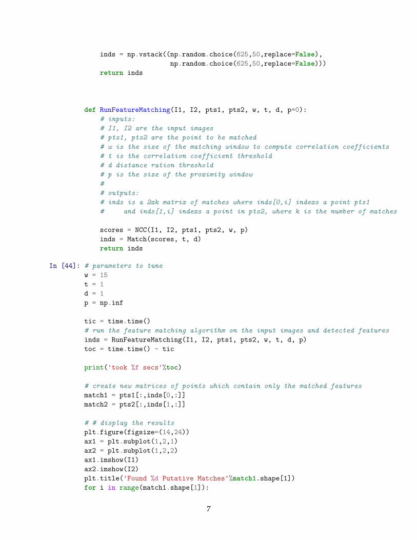
def RunFeatureMatching(I1, I2, pts1, pts2, w, t, d, p=0):# inputs:# I1, I2 are the input images# pts1, pts2 are the point to be matched# w is the size of the matching window to compute correlation coefficients# t is the correlation coefficient threshold# d distance ration threshold# p is the size of the proximity window## outputs:# inds is a 2xk matrix of matches where inds[0,i] indexs a point pts1# and inds[1,i] indexs a point in pts2, where k is the number of matches

scores = NCC(I1, I2, pts1, pts2, w, p)inds = Match(scores, t, d)return inds

In [44]: # parameters to tunew = 15t = 1d = 1p = np.inf

tic = time.time()# run the feature matching algorithm on the input images and detected featuresinds = RunFeatureMatching(I1, I2, pts1, pts2, w, t, d, p)toc = time.time() - tic

print('took %f secs'%toc)

# create new matrices of points which contain only the matched featuresmatch1 = pts1[:,inds[0,:]]match2 = pts2[:,inds[1,:]]

# # display the resultsplt.figure(figsize=(14,24))ax1 = plt.subplot(1,2,1)ax2 = plt.subplot(1,2,2)ax1.imshow(I1)ax2.imshow(I2)plt.title('Found %d Putative Matches'%match1.shape[1])for i in range(match1.shape[1]):

7

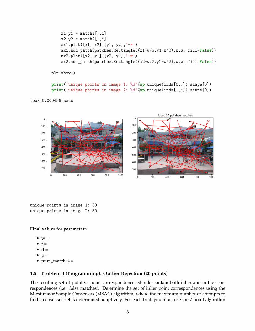
x1,y1 = match1[:,i]x2,y2 = match2[:,i]ax1.plot([x1, x2],[y1, y2],'-r')ax1.add_patch(patches.Rectangle((x1-w/2,y1-w/2),w,w, fill=False))ax2.plot([x2, x1],[y2, y1],'-r')ax2.add_patch(patches.Rectangle((x2-w/2,y2-w/2),w,w, fill=False))

plt.show()

print('unique points in image 1: %d'%np.unique(inds[0,:]).shape[0])print('unique points in image 2: %d'%np.unique(inds[1,:]).shape[0])

took 0.000456 secs

unique points in image 1: 50unique points in image 2: 50

Final values for parameters

• w =• t =• d =• p =• num_matches =

1.5 Problem 4 (Programming): Outlier Rejection (20 points)

The resulting set of putative point correspondences should contain both inlier and outlier cor-respondences (i.e., false matches). Determine the set of inlier point correspondences using theM-estimator Sample Consensus (MSAC) algorithm, where the maximum number of attempts tofind a consensus set is determined adaptively. For each trial, you must use the 7-point algorithm

8

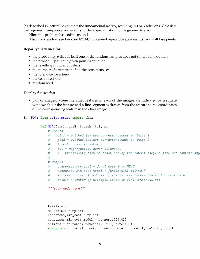
(as described in lecture) to estimate the fundamental matrix, resulting in 1 or 3 solutions. Calculatethe (squared) Sampson error as a first order approximation to the geometric error.

Hint: this problem has codimension 1Also: fix a random seed in your MSAC. If I cannot reproduce your results, you will lose points.

Report your values for:

• the probability p that as least one of the random samples does not contain any outliers• the probability α that a given point is an inlier• the resulting number of inliers• the number of attempts to find the consensus set• the tolerance for inliers• the cost threshold• random seed

Display figures for:

• pair of images, where the inlier features in each of the images are indicated by a squarewindow about the feature and a line segment is drawn from the feature to the coordinatesof the corresponding feature in the other image

In [50]: from scipy.stats import chi2

def MSAC(pts1, pts2, thresh, tol, p):# Inputs:# pts1 - matched feature correspondences in image 1# pts2 - matched feature correspondences in image 2# thresh - cost threshold# tol - reprojection error tolerance# p - probability that as least one of the random samples does not contain any outliers## Output:# consensus_min_cost - final cost from MSAC# consensus_min_cost_model - fundamental matrix F# inliers - list of indices of the inliers corresponding to input data# trials - number of attempts taken to find consensus set

"""your code here"""

trials = 0max_trials = np.infconsensus_min_cost = np.infconsensus_min_cost_model = np.zeros((3,4))inliers = np.random.randint(0, 200, size=100)return consensus_min_cost, consensus_min_cost_model, inliers, trials

9

# MSAC parametersthresh = 0tol = 0p = 0alpha = 0

tic=time.time()

cost_MSAC, F_MSAC, inliers, trials = MSAC(pts1, pts2, thresh, tol, p)

# choose just the inliersx1 = pts1[:,inliers]x2 = pts2[:,inliers]outliers = np.setdiff1d(np.arange(pts1.shape[1]),inliers)

toc=time.time()time_total=toc-tic

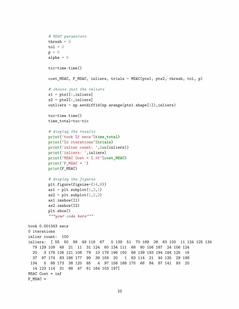
# display the resultsprint('took %f secs'%time_total)print('%d iterations'%trials)print('inlier count: ',len(inliers))print('inliers: ',inliers)print('MSAC Cost = %.9f'%cost_MSAC)print('F_MSAC = ')print(F_MSAC)

# display the figuresplt.figure(figsize=(14,8))ax1 = plt.subplot(1,2,1)ax2 = plt.subplot(1,2,2)ax1.imshow(I1)ax2.imshow(I2)plt.show()"""your code here"""

took 0.001343 secs0 iterationsinlier count: 100inliers: [ 55 50 99 49 116 67 0 139 51 70 189 28 83 100 11 124 125 134

79 129 109 48 21 11 31 124 60 134 111 68 80 156 187 24 156 12420 3 178 126 121 108 79 10 178 196 150 68 139 193 194 184 125 1637 97 174 83 186 177 99 39 159 20 1 83 114 21 40 135 29 198

134 5 88 173 38 120 85 4 97 158 188 170 66 84 87 141 93 2014 123 114 31 88 47 61 164 103 197]

MSAC Cost = infF_MSAC =

10

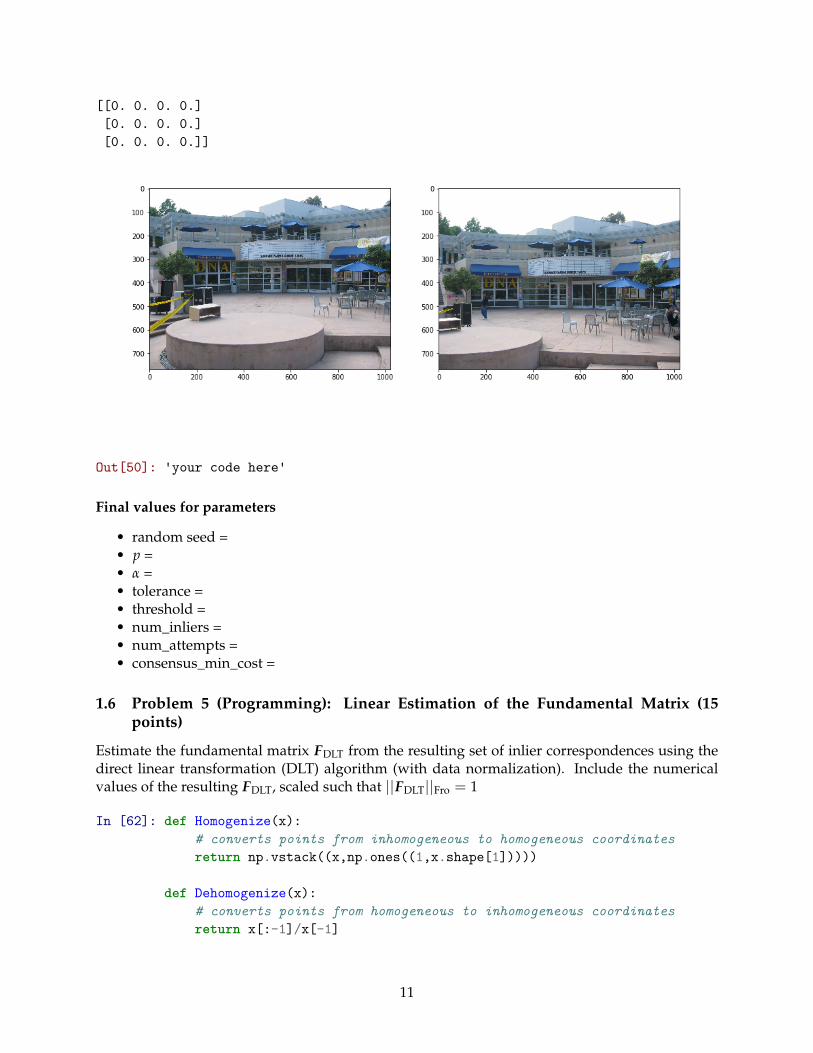
[[0. 0. 0. 0.][0. 0. 0. 0.][0. 0. 0. 0.]]

Out[50]: 'your code here'

Final values for parameters

• random seed =• p =• α =• tolerance =• threshold =• num_inliers =• num_attempts =• consensus_min_cost =

1.6 Problem 5 (Programming): Linear Estimation of the Fundamental Matrix (15points)

Estimate the fundamental matrix FDLT from the resulting set of inlier correspondences using thedirect linear transformation (DLT) algorithm (with data normalization). Include the numericalvalues of the resulting FDLT, scaled such that ||FDLT||Fro = 1

In [62]: def Homogenize(x):# converts points from inhomogeneous to homogeneous coordinatesreturn np.vstack((x,np.ones((1,x.shape[1]))))

def Dehomogenize(x):# converts points from homogeneous to inhomogeneous coordinatesreturn x[:-1]/x[-1]

11

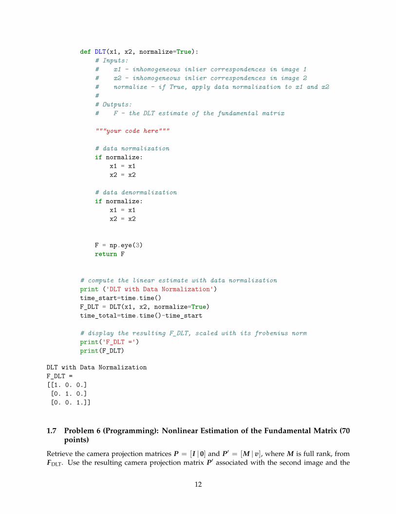
def DLT(x1, x2, normalize=True):# Inputs:# x1 - inhomogeneous inlier correspondences in image 1# x2 - inhomogeneous inlier correspondences in image 2# normalize - if True, apply data normalization to x1 and x2## Outputs:# F - the DLT estimate of the fundamental matrix

"""your code here"""

# data normalizationif normalize:

x1 = x1x2 = x2

# data denormalizationif normalize:

x1 = x1x2 = x2

F = np.eye(3)return F

# compute the linear estimate with data normalizationprint ('DLT with Data Normalization')time_start=time.time()F_DLT = DLT(x1, x2, normalize=True)time_total=time.time()-time_start

# display the resulting F_DLT, scaled with its frobenius normprint('F_DLT =')print(F_DLT)

DLT with Data NormalizationF_DLT =[[1. 0. 0.][0. 1. 0.][0. 0. 1.]]

1.7 Problem 6 (Programming): Nonlinear Estimation of the Fundamental Matrix (70points)

Retrieve the camera projection matrices P = [I | 0] and P′ = [M | v], where M is full rank, fromFDLT. Use the resulting camera projection matrix P′ associated with the second image and the

12

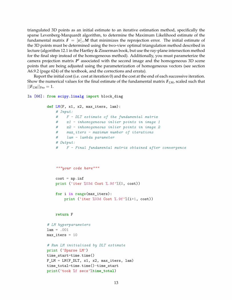
triangulated 3D points as an initial estimate to an iterative estimation method, specifically thesparse Levenberg-Marquardt algorithm, to determine the Maximum Likelihood estimate of thefundamental matrix F = [v]×M that minimizes the reprojection error. The initial estimate ofthe 3D points must be determined using the two-view optimal triangulation method described inlecture (algorithm 12.1 in the Hartley & Zisserman book, but use the ray-plane intersection methodfor the final step instead of the homogeneous method). Additionally, you must parameterize thecamera projection matrix P′ associated with the second image and the homogeneous 3D scenepoints that are being adjusted using the parameterization of homogeneous vectors (see sectionA6.9.2 (page 624) of the textbook, and the corrections and errata).

Report the initial cost (i.e. cost at iteration 0) and the cost at the end of each successive iteration.Show the numerical values for the final estimate of the fundamental matrix FLM, scaled such that||FLM||Fro = 1.

In [66]: from scipy.linalg import block_diag

def LM(F, x1, x2, max_iters, lam):# Input:# F - DLT estimate of the fundamental matrix# x1 - inhomogeneous inlier points in image 1# x2 - inhomogeneous inlier points in image 2# max_iters - maximum number of iterations# lam - lambda parameter# Output:# F - Final fundamental matrix obtained after convergence

"""your code here"""

cost = np.infprint ('iter %03d Cost %.9f'%(0, cost))

for i in range(max_iters):print ('iter %03d Cost %.9f'%(i+1, cost))

return F

# LM hyperparameterslam = .001max_iters = 10

# Run LM initialized by DLT estimateprint ('Sparse LM')time_start=time.time()F_LM = LM(F_DLT, x1, x2, max_iters, lam)time_total=time.time()-time_startprint('took %f secs'%time_total)

13

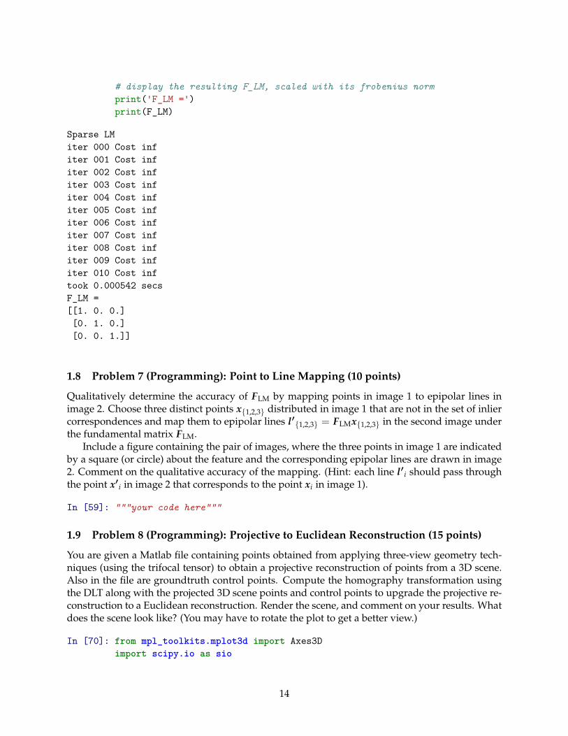
# display the resulting F_LM, scaled with its frobenius normprint('F_LM =')print(F_LM)

Sparse LMiter 000 Cost infiter 001 Cost infiter 002 Cost infiter 003 Cost infiter 004 Cost infiter 005 Cost infiter 006 Cost infiter 007 Cost infiter 008 Cost infiter 009 Cost infiter 010 Cost inftook 0.000542 secsF_LM =[[1. 0. 0.][0. 1. 0.][0. 0. 1.]]

1.8 Problem 7 (Programming): Point to Line Mapping (10 points)

Qualitatively determine the accuracy of FLM by mapping points in image 1 to epipolar lines inimage 2. Choose three distinct points x{1,2,3} distributed in image 1 that are not in the set of inliercorrespondences and map them to epipolar lines l′{1,2,3} = FLMx{1,2,3} in the second image underthe fundamental matrix FLM.

Include a figure containing the pair of images, where the three points in image 1 are indicatedby a square (or circle) about the feature and the corresponding epipolar lines are drawn in image2. Comment on the qualitative accuracy of the mapping. (Hint: each line l′i should pass throughthe point x′i in image 2 that corresponds to the point xi in image 1).

In [59]: """your code here"""

1.9 Problem 8 (Programming): Projective to Euclidean Reconstruction (15 points)

You are given a Matlab file containing points obtained from applying three-view geometry tech-niques (using the trifocal tensor) to obtain a projective reconstruction of points from a 3D scene.Also in the file are groundtruth control points. Compute the homography transformation usingthe DLT along with the projected 3D scene points and control points to upgrade the projective re-construction to a Euclidean reconstruction. Render the scene, and comment on your results. Whatdoes the scene look like? (You may have to rotate the plot to get a better view.)

In [70]: from mpl_toolkits.mplot3d import Axes3Dimport scipy.io as sio

14

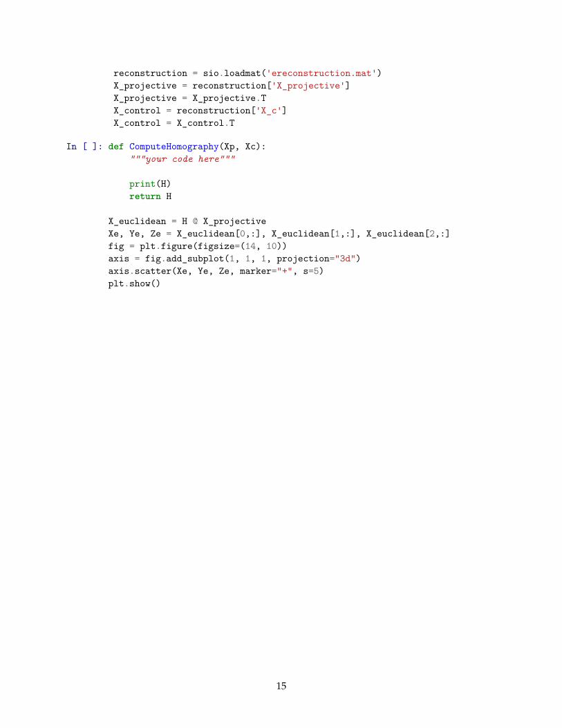
reconstruction = sio.loadmat('ereconstruction.mat')X_projective = reconstruction['X_projective']X_projective = X_projective.TX_control = reconstruction['X_c']X_control = X_control.T

In [ ]: def ComputeHomography(Xp, Xc):"""your code here"""

print(H)return H

X_euclidean = H @ X_projectiveXe, Ye, Ze = X_euclidean[0,:], X_euclidean[1,:], X_euclidean[2,:]fig = plt.figure(figsize=(14, 10))axis = fig.add_subplot(1, 1, 1, projection="3d")axis.scatter(Xe, Ye, Ze, marker="+", s=5)plt.show()

15