ASSESSMENT OF THE PETROLEUM GENERATION POTENTIAL OF THE NEAL SHALE

IN THE BLACK WARRIOR BASIN, ALABAMA

by

JOEL ARTHUR LEGG

RONA J. DONAHOE, COMMITTEE CHAIR

ANDREW M. GOODLIFFE

JACK C. PASHIN

YUEHAN LU

A THESIS

Submitted in partial fulfillment of the requirements

for the degree of Master of Science

in the Department of Geological Sciences

in the Graduate School of

The University of Alabama

TUSCALOOSA, ALABAMA

2014

Copyright Joel Arthur Legg 2014

ALL RIGHTS RESERVED

ii

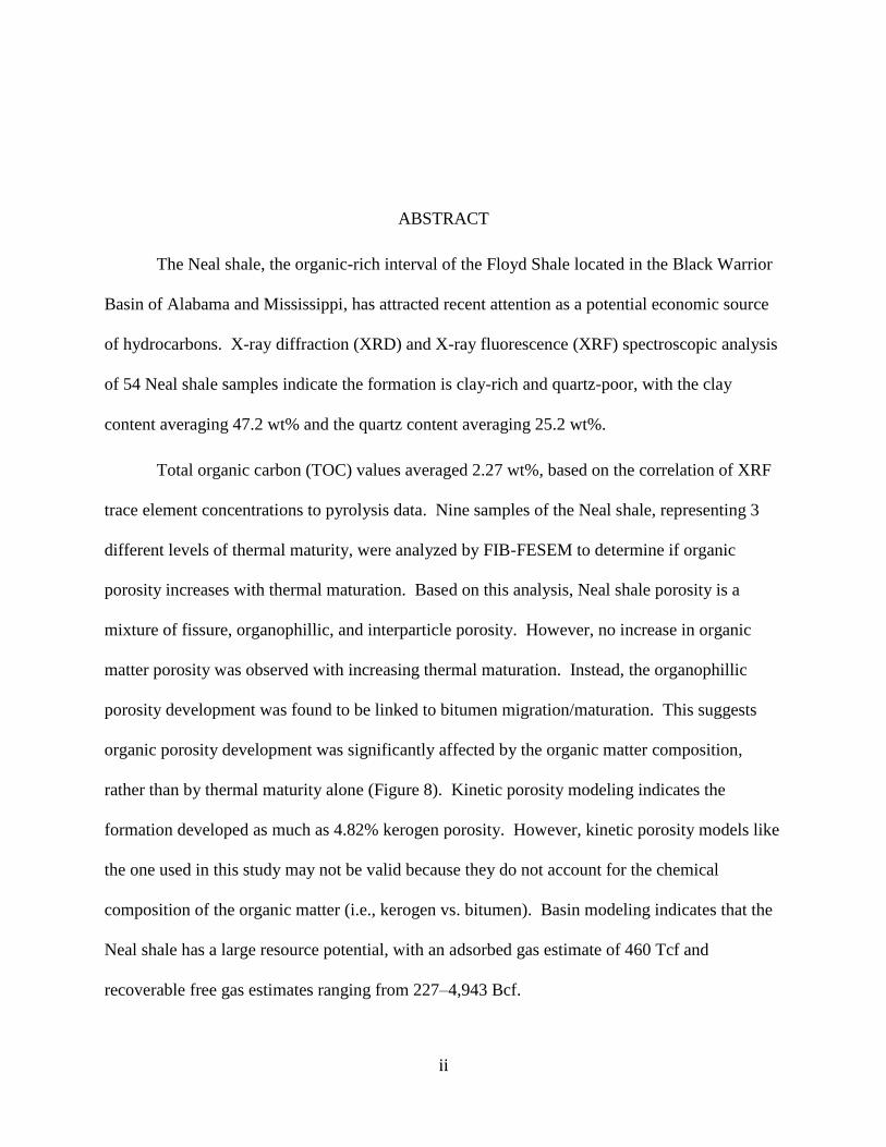
ABSTRACT

The Neal shale, the organic-rich interval of the Floyd Shale located in the Black Warrior

Basin of Alabama and Mississippi, has attracted recent attention as a potential economic source

of hydrocarbons. X-ray diffraction (XRD) and X-ray fluorescence (XRF) spectroscopic analysis

of 54 Neal shale samples indicate the formation is clay-rich and quartz-poor, with the clay

content averaging 47.2 wt% and the quartz content averaging 25.2 wt%.

Total organic carbon (TOC) values averaged 2.27 wt%, based on the correlation of XRF

trace element concentrations to pyrolysis data. Nine samples of the Neal shale, representing 3

different levels of thermal maturity, were analyzed by FIB-FESEM to determine if organic

porosity increases with thermal maturation. Based on this analysis, Neal shale porosity is a

mixture of fissure, organophillic, and interparticle porosity. However, no increase in organic

matter porosity was observed with increasing thermal maturation. Instead, the organophillic

porosity development was found to be linked to bitumen migration/maturation. This suggests

organic porosity development was significantly affected by the organic matter composition,

rather than by thermal maturity alone (Figure 8). Kinetic porosity modeling indicates the

formation developed as much as 4.82% kerogen porosity. However, kinetic porosity models like

the one used in this study may not be valid because they do not account for the chemical

composition of the organic matter (i.e., kerogen vs. bitumen). Basin modeling indicates that the

Neal shale has a large resource potential, with an adsorbed gas estimate of 460 Tcf and

recoverable free gas estimates ranging from 227–4,943 Bcf.

iii

Uniaxial strength tests indicate Neal shale samples have an average unconfined axial

strength of 3.42 MPa, and the underlying Lewis Limestone samples have an average unconfined

diametral strength of 22.22 MPa. This suggests that the underlying Lewis Limestone should

serve as an active barrier to hydraulic fracturing efforts within the Neal shale. Although the Neal

shale has retained a large volume of natural gas, mapping of the limestone fracture barriers and

additional testing of hydraulic fracturing mechanics on clay-rich formations will be necessary

before the potential development of the Neal shale as an unconventional petroleum reservoir can

be fully evaluated.

iv

DEDICATION

I would like to dedicate this work to my father who taught me the value of hard work and

what it takes to succeed.

v

LIST OF ABBREVIATIONS AND SYMBOLS

ASTM American Standard for Testing and Materials

Bcf Billion Cubic Feet

BSE Back-Scattered Electron

CC Convertible Carbon

CR Residual Carbon

EDS Energy Dispersive Spectroscopy

FESEM Field Emission Scanning Electron Microscope

FIB Focused Ion Beam

FIB-FESEM Focused Ion Beam coupled with a Field Emission Scanning Electron Microscope

ft Feet

HI Hydrogen Index

HIo Original Hydrogen Index

HIpd Present Day Hydrogen Index

km Kilometer

MMbo Million Barrels of Oil

MPa Mega-Pascal

vi

nm Nanometer

OI Oxygen Index

PI Production Index

PIo Original Production Index

PIpd Present Day Production Index

r Correlation Coefficient

R2 Coefficient of Determination

RhoK Kerogen Density

RhoB Bulk Density

Ro Vitrinite Reflectance in Oil

SE Secondary Electron

SEM Scanning Electron Microscope

Tcf Trillion Cubic Feet

TOC Total Organic Carbon

TOCo Original Total Organic Carbon

TOCpd Present Day Total Organic Carbon

TR Transformation Ratio

vii

TRHI Transformation Ratio based on the Hydrogen Index

TTI Time Temperature Index

wt% Weight Percent

XRD X-ray Diffraction diffractometer/diffraction

XRF X-ray Florescence spectrometer/spectrometry

viii

ACKNOWLEDGMENTS

I would like to thank my thesis committee, Dr. Rona Donahoe, Dr. Jack Pashin, Dr.

Andrew Goodliffe, and Dr. Yuehan Lu for their guidance and assistance during the process of

conducting this study. I would also like to thank Rich Martens for all of his help and guidance in

the FIB-FESEM work. If not for his knowledge and expertise, that aspect of this study would

not have been accomplished. In addition, I would like to thank Marcella McIntyre and Tony

Smithson for sharing their technical expertise with me.

Finally I would like to thank my wife, Amy, for always being there and supporting me

through this long journey. I cherish the love and support you have shown me through this time.

ix

CONTENTS

ABSTRACT ...................................................................................................................... ii

DEDICATION ................................................................................................................. iv

LIST OF ABBREVIATIONS AND SYMBOLS .............................................................. v

ACKNOWLEDGMENTS ............................................................................................. viii

LIST OF TABLES ........................................................................................................... xi

LIST OF FIGURES ........................................................................................................ xii

1 INTRODUCTION ....................................................................................................... 1

1.1 Background .............................................................................................................. 1

1.2 Motivation ................................................................................................................ 9

2 METHODS ................................................................................................................ 10

2.1 XRD and XRF Sample Crushing ........................................................................... 11

2.2 XRD Analysis ......................................................................................................... 12

2.3 XRF ........................................................................................................................ 14

2.4 Strength Test .......................................................................................................... 14

2.5 FESEM ................................................................................................................... 15

2.5.1 FESEM Sample Preparation ......................................................................................... 16

2.5.2 FESEM Analysis ........................................................................................................... 17

2.5.3 FESEM 3-D Image Reconstruction ............................................................................... 18

2.6 Modeling ............................................................................................................... 19

2.6.1 Kinetic Porosity Modeling ............................................................................................ 20

x

2.6.2 Basin Modeling ............................................................................................................. 22

2.7 Volumetric Analysis .............................................................................................. 23

3 RESULTS .................................................................................................................. 24

3.1 XRD Results .......................................................................................................... 24

3.2 XRF Results ........................................................................................................... 25

3.3 Strength Test Results ............................................................................................. 29

3.4 FESEM Results ...................................................................................................... 30

3.5 Modeling Results ................................................................................................... 35

3.5.1 Kinetic Porosity ............................................................................................................ 35

3.5.2 Basin Modeling ............................................................................................................. 36

4 DISCUSSION ............................................................................................................ 47

4.1 Mineralogy ............................................................................................................. 47

4.2 Strength Test .......................................................................................................... 49

4.3 Organic Porosity .................................................................................................... 50

4.4 Volumetric Analysis .............................................................................................. 53

5 CONCLUSIONS ........................................................................................................ 55

REFERENCES ................................................................................................................ 56

APPENDIX ..................................................................................................................... 60

xi

LIST OF TABLES

Table 1. Comparison of TOC values estimated from XRF Cr+Mo+Ni concentration

with measured TOC values from Pashin et al. (2011) . .................................................... 28

Table 2. Results of FESEM 3-D reconstruction analysis of Neal shale samples,

reported in volume percent .............................................................................................. 35

Table 3. Table of calculated kerogen porosity including input data ................................ 36

Table 4. Recoverable free gas estimates and adsorbed gas-in-place based on risk

analysis and basin modeling ............................................................................................ 53

Table A-1. Geochemical Data for the Neal shale ............................................................ 60

Table A-2. XRD results for Well 2191 samples .............................................................. 61

Table A-3. XRD results for Well 1780 samples .............................................................. 62

Table A-4. XRD results for Well 15668 samples ............................................................ 63

Table A-5. XRF results for Well 2191 samples ............................................................... 64

Table A-6. XRF results for Well 1780 samples ............................................................... 66

Table A-7. XRF results for Well 15668 samples ............................................................. 68

Table A-8. XRF trace element data for samples from Well 2191 ................................... 69

Table A-9. XRF trace element data for samples from Well 1780 ................................... 71

Table A-10. XRF trace element data for samples from Well 15668 ................................ 72

Table A-11. Uniaxial stength test results for Well 15668 core samples ........................... 73

Table A-12. TerraTek

XRD analysis of Well 15668 for the Geological Survey of

Alabama study by Pashin et al. (2011) ............................................................................ 75

xii

LIST OF FIGURES

Figure 1. Isopach map of the Neal shale of the Black Warrior Basin ................................ 3

Figure 2. Location of the Black Warrior Basin in relation to tectonics, including the

three counties in Alabama where the wells used in this study are located ........................ 6

Figure 3. Regional cross-section showing the facies relationships in Devonian-

Mississippian strata of the Black Warrior Basin ................................................................ 8

Figure 4. Sample 9044.0 from Well 15668 showing the ridge necessary to rapidly find

the coincidence point of the FIB-FESEM ........................................................................ 16

Figure 5. Sample 9044.0 from Well 15668 showing the trench milled on both sides of

the area of interest and the flattened top .......................................................................... 18

Figure 6. Graph of TOC values obtained by pyrolysis (Pashin et al., 2011) vs.

Cr+Mo+Ni concentrations, determined for the Neal shale samples by XRF analysis .... 27

Figure 7. EDS maps of Neal shale 2920-25 ft sample showing the location of organic

matter (blue arrow) and a pyrite framboid (red arrow) .................................................... 32

Figure 8. Image of Neal shale 3000-05 ft sample collected using the BSE detector (left)

and the SE detector (right) ............................................................................................... 33

Figure 9. 3-D models of Neal Floyd 3000-05 ft sample showing the reconstructed

sample using A) the BSE detector, B) the SE detector, C) reconstructed organic matter,

D) porosity, and E) pyrite with the scale bar in micrometers .......................................... 34

Figure 10. Easy %Ro values for Well 2191 ..................................................................... 37

Figure 11. Easy %Ro values for Well 1780 ..................................................................... 38

Figure 12. Easy %Ro values for Well 15668 ................................................................... 39

Figure 13. Burial history of Well 2191, including Easy %Ro values as an

overlay .............................................................................................................................. 40

Figure 14. Burial history of Well 1780, including Easy %Ro values as an

overlay .............................................................................................................................. 41

xiii

Figure 15. Burial history of Well 15668, including Easy %Ro values as an

overlay .............................................................................................................................. 42

Figure 16. Transformation ratio of the kerogen within the Neal shale ............................ 43

Figure 17. Burial history of Well 2191 with overlain hydrocarbon zones ...................... 44

Figure 18. Burial history of Well 1780 with overlain hydrocarbon zones ...................... 45

Figure 19. Burial history of Well 15668 with overlain hydrocarbon zones .................... 46

Figure A-1. Correlation coefficient matrix for the Neal shale ......................................... 76

Figure A-2. Correlation coefficient matrix for the Lewis Limestone .............................. 77

1

1 INTRODUCTION

For each potential shale play, a comprehensive petrologic analysis needs to be performed

to fully understand the degree to which porosity, hydrocarbon content, and mineralogy vary, so

that production can be maximized. If the shale unit is thoroughly characterized, informed

decisions can be made about the drilling and completion technologies to be used in developing

the reservoir. Successful evaluation of the potential economic viability of the Neal shale

includes verifying the amount of gas-in-place, the mineralogy, and the pressure of the formation

(Pashin, 2008). By analyzing the development of nanoporosity within organic matter as a

function of thermal maturation, its contribution to the total porosity of the Neal shale can be

determined. Analyzing the mineralogy of the formation allows for sweet-spot identification for

landing laterals and designing completion programs. If the Neal shale has generated and

maintained sufficient volumes of hydrocarbons and the mineralogy is suitable for hydraulic

fracturing, production of this resource could assist in the U.S. goal of energy independence. In

addition, results from this study will assist in understanding the development of organic porosity

and thus enable better modeling for other shale plays.

1.1 Background

The Neal shale has been identified as a potential unconventional hydrocarbon reservoir

within the Black Warrior Basin of Alabama and Mississippi (Pashin et al., 2011). The Neal

shale is an informal term for the organic-rich interval of the Floyd Shale and ranges in thickness

from less than 25 feet to 350 feet in Alabama (Figure 1). This zone may be a viable target for

economic hydrocarbon production (Pashin et al., 2011). Petroleum exploration companies have

had limited success using vertical wells within the Neal shale; horizontal wells will likely be

2

necessary for economic production, due to the limited thickness of the unit (Pashin, 2008). To

date, companies targeting the organic-rich shale have drilled near faults; however, wells that

have been drilled near faults in the stratigraphically equivalent Barnett Shale of the Fort Worth

Basin have resulted in low returns, compared to those of other areas (Bowker, 2003). This is due

to the presence of macro-fractures that are filled with carbonate cement which make the shale

less responsive to stimulation efforts (Bowker, 2003). In addition, low returns near fault zones

may be caused by diversion of the hydraulic fracture fluid along these preexisting pathways thus

diverting energy away from the target formation.

Carroll et al. (1995) studied the burial history and source rock characteristics of the Neal

shale, based on measured mean-maximum vitrinite reflectance in oil values (Ro). From this

information, time temperature index (TTI) values were calculated using Lopatin’s method to

determine the petroleum generation history of the Neal shale. An average geothermal gradient of

16°F/1000 ft (-8.9°C/304.8 m) was used in the TTI calculations. Lopatin’s TTI method

(Lopatin, 1971) was originally calibrated based on Type III kerogen and only takes into account

the temperature at depth and amount of time the formation of interest was buried. This model

does not suffice for the Neal shale, which is dominated by Type II kerogen (Carroll et al., 1995;

Pashin et al., 2011) and has a complex tectonic history. Kinetic modeling of the chemical

reactions that took place over time, as incorporated into Petromod® software, can be used to

model the timing and volume of hydrocarbons generated from the formation. In addition,

Petromod®

calculates Easy %Ro values using the Sweeney and Burnham (1990) method which

allows for correlation to measured Ro values. The Sweeney and Burnham (1990) method of

calculating Ro is based on running 20 parallel first-order Arrhenius chemical reactions which

control vitrinite maturation.

3

Figure 1: Isopach map of the Neal shale of the Black Warrior Basin (modified from Pashin et al.,

2011).

The use of scanning electron microscopy (SEM) has led to better understanding of

organic porosity development. The relationship of organic porosity to thermal maturity has been

studied by Curtis et al. (2010, 2011, 2012, and 2013), Sondergeld et al. (2010), Modica and

4

Lapierre (2012), Bernard et al. (2012), and Ambrose et al. (2012), amongst others. Some of

these studies have shown an increase in porosity with thermal maturation, but the mathematical

nature of that relationship is undetermined. In addition, Curtis et al. (2012) showed that porosity

development may not be linked to thermal maturity alone, but may also be related to the

chemical makeup of the macerals.

A kinetic model of porosity development may be employed without the use of SEM. A

kinetic model for assessing kerogen porosity was developed by Modica and Lapierre (2012).

Their model utilizes geochemical data collected through pyrolysis studies to determine kerogen

porosity. The mathematical model uses the original amount of total organic carbon (TOCo), the

present day TOC (TOCpd), the labile portion of TOC termed ‘convertible carbon’ (Cc), the

transformation ratio (TR), and the density of both kerogen (RhoK) and the inorganic matrix

(RhoB). However, this model may not be adequate for all systems, based on a study by Curtis et

al. (2012) that found that separate pieces of organic matter at the same level of maturity did not

have the same proportion of porosity development.

In the Barnett Shale of Texas, mineralogy may be the deciding factor controlling the best

well locations (Bowker, 2003). The best production in the Barnett Shale occurs where the shale

contains more than 45 weight percent (wt%) quartz and less than 27 wt% clay (Bowker, 2003).

This is due to the higher quartz content making the formation sufficiently brittle to fracture, thus

allowing a linkage between the wellbore and shale micro-porosity.

The mechanisms controlling the quality of the source rock depend on tectonics,

stratigraphy and sedimentation, burial history, and other geologic processes (McCarthy et al.,

2011; Pashin et al., 2011). Because of this, a brief overview of these facets as they pertain to the

5

deposition and organic richness of the Neal shale will allow a more in-depth interpretation of the

study results.

The Black Warrior Basin is a Paleozoic foreland basin that formed due to extensional and

compressional tectonic settings (Pashin et al., 2011). The Paleozoic basin formed adjacent to the

intersection of the Appalachian and Ouachita orogenic belts (Thomas et al., 1977, 1988; Pashin

et al., 2011), and includes a triangular area in northwestern Alabama and northeastern

Mississippi. The Basin is bordered on the southeast by the Appalachian Orogeny, on the

southwest by the Ouachita Orogeny, and on the north by the Nashville Dome (Figure 2) (Carroll

et al., 1995). The Basin is mainly a Ouachita foreland basin; Appalachian thrust and sediment

loads did not deposit on the southeastern portion of the Basin until the Early Pennsylvanian

(Pashin, 2004).

The tectonic history of the Black Warrior Basin can be summarized by 6 stages,

according to Thomas (1988):

1) Late Precambrian – Early Cambrian: Iapetan rifting with the associated deposition

of muddy, calcareous clastic sediment;

2) Middle Cambrian – Mississippian: development of a passive continental margin

with deposition of shallow-water carbonates;

3) Late Mississippian: initial Ouachita orogenesis with deposition of a mixed

carbonate-siliciclastic succession;

4) Early – Late Pennsylvanian: maximum basin subsidence associated with the

Appalachian-Ouachita orogeneisis (Pashin, 1994) and deposition of synorogenic

sediment; progradation of thick, coal-bearing siliciclastic successions from source

areas in the Appalachian-Ouachita orogen.

6

5) Late Pennsylvanian – Early Mesozoic: uplift resulting in Permian-Cretaceous

erosion and non-deposition (Telle et al., 1987);

6) Mesozoic: transgressive marine sediments of the Mississippi embayment

onlapped the passive margin-shelf.

Figure 2: Location of the Black Warrior Basin in relation to tectonics, including the three

counties in Alabama where the wells used in this study are located (modified from Pawlewicz

and Hatch, 2007)

7

The Black Warrior Basin is a structural homocline that dips southwest toward the

Ouachita Orogen and is broken by extensional faults, which show multiphase tectonic

development that spanned the Paleozoic Era (Thomas, 1988; Groshong et al., 2010; Pashin et al.,

2011). The geologic structure of the Black Warrior Basin affects the geometry, continuity, and

permeability of shale reservoirs (Pashin et al., 2011). Faults within the Basin pose a significant

risk for leak-off of stimulation fluid during hydraulic fracturing (Pashin et al., 2011) that would

hinder fracture stimulation efforts. Thus, care must be taken to avoid drilling near fault zones.

The Neal shale was deposited as part of the Chester Group Floyd Shale in the Black

Warrior Basin during the Upper Mississippian Period. The Neal shale, the object of recent shale

gas exploration, is the organic-rich interval of the clastic wedge that deposited at the toe of the

ramp (Figure 3). The formation sediment was transported towards the southeast along

depositional strike of the Warrior platform, and deposited in epeiric ramp and basinal

environments during the Late Mississippian. The Neal shale is in a complex facies relationship

with strata of the Pride Mountain Formation, Hartselle Sandstone, Bangor Limestone, and lower

Parkwood Formation (Pashin, 2008) with the majority of the Neal shale being equivalent to the

Bangor Limestone. Individual parasequences thin towards the southwest and define a clinoform

stratal geometry in which near-shore facies of the Pride Mountain-Bangor interval pass into

condensed, starved-basin facies of the Neal shale (Pashin, 2008). Overlying Pottsville sediments

had a principal source to the southeast of the Black Warrior Basin and represents the thick clastic

wedge shed from the Appalachian orogenic belt (Pashin and Raymond, 2004). Pottsville

deposition caused the foreland basin to rapidly subside during the Pennsylvanian-Early Permian

(Cleaves and Broussard, 1980).

8

Figure 3: Regional cross-section showing the facies relationships in Devonian-Mississippian

strata of the Black Warrior Basin (from Pashin et al., 2011)

The Neal shale is an organic-rich silty, calcareous, laminated to thick-bedded shale

formation that was deposited in slope and epeiric basin floor environments (Pashin et al., 2011).

Processes occurring within the basin were varied and influenced by the development of

carbonate ramps, siliciclastic coastal plains and marine shelves (Pashin et al., 2011). Deposition

of the Neal shale was highly dynamic, reflecting changing redox conditions, variable sediment

and nutrient flux, and reworking by storms, which resulted in heterogeneous facies and reservoir

quality (Pashin et al., 2011). The Neal shale also contains thin interbeds of limestone and

siltstone, that are wavy or lenticlular and contain ripple cross-laminae (Pashin et al., 2011).

9

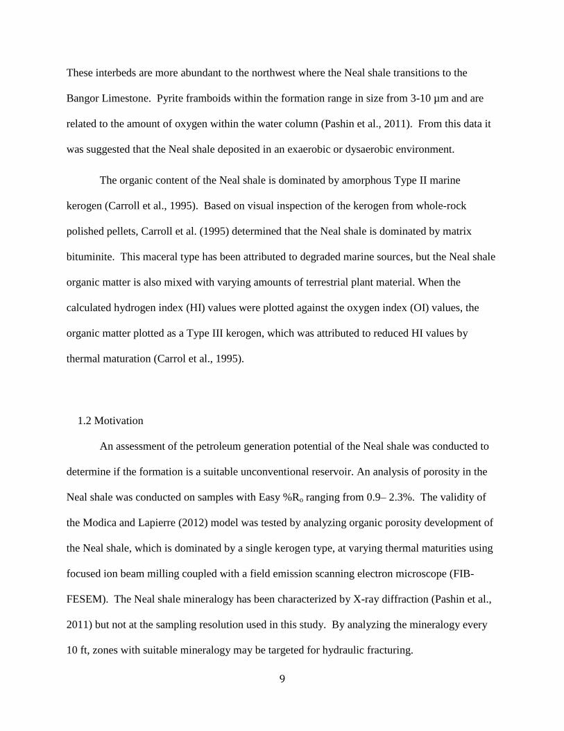
These interbeds are more abundant to the northwest where the Neal shale transitions to the

Bangor Limestone. Pyrite framboids within the formation range in size from 3-10 µm and are

related to the amount of oxygen within the water column (Pashin et al., 2011). From this data it

was suggested that the Neal shale deposited in an exaerobic or dysaerobic environment.

The organic content of the Neal shale is dominated by amorphous Type II marine

kerogen (Carroll et al., 1995). Based on visual inspection of the kerogen from whole-rock

polished pellets, Carroll et al. (1995) determined that the Neal shale is dominated by matrix

bituminite. This maceral type has been attributed to degraded marine sources, but the Neal shale

organic matter is also mixed with varying amounts of terrestrial plant material. When the

calculated hydrogen index (HI) values were plotted against the oxygen index (OI) values, the

organic matter plotted as a Type III kerogen, which was attributed to reduced HI values by

thermal maturation (Carrol et al., 1995).

1.2 Motivation

An assessment of the petroleum generation potential of the Neal shale was conducted to

determine if the formation is a suitable unconventional reservoir. An analysis of porosity in the

Neal shale was conducted on samples with Easy %Ro ranging from 0.9– 2.3%. The validity of

the Modica and Lapierre (2012) model was tested by analyzing organic porosity development of

the Neal shale, which is dominated by a single kerogen type, at varying thermal maturities using

focused ion beam milling coupled with a field emission scanning electron microscope (FIB-

FESEM). The Neal shale mineralogy has been characterized by X-ray diffraction (Pashin et al.,

2011) but not at the sampling resolution used in this study. By analyzing the mineralogy every

10 ft, zones with suitable mineralogy may be targeted for hydraulic fracturing.

10

2 METHODS

FIB-FESEM was used to analyze the development of organic porosity as a function of

thermal maturation using samples of the Neal shale selected from cores/cuttings of three wells

located in Alabama (Figure 1). Cuttings from Wells 2191 and 1780 were collected at 5-ft

intervals and 10-ft intervals respectively during the drilling process. These cuttings samples will

thus be referred to by their sample depth range. These samples were obtained from the sample

collection of the Geological Survey of Alabama. The wells chosen for this study are the Gilmer

17-12 #1 well (permit number 2191) located in Lamar County, the Ralph W. Holliman #13-16

well (permit number 1780) located in Pickens County, and the Lamb 1-3 No.1 well (permit

number 15668) located in Greene County, Alabama. These wells will subsequently be identified

by their permit number (e.g., Well 15668). A total of 54 samples of the Neal Shale, 6 samples of

the Floyd Shale, and 4 samples of the Lewis Limestone were obtained from the core collection of

the Geological Survey of Alabama. Only rock cuttings were available from Wells 2191 and

1780 (sampled at 10-ft intervals). Hereafter, the cuttings samples will be referred to by their

sample depth range (e.g., 2740-45 ft). While drilling Well 15668, a 25 ft core of the Neal shale

was collected. The core was sampled approximately every 10 ft to correlate with the cuttings

sampled from the other two wells. Within Wells 2191 and 1780, measured vitrinite reflectance

values ranged from 0.92– 0.98% and 1.44– 1.59%, respectively, according to data previously

published by Carroll et al. (1995). Within Well 15668, calculated Easy %Ro values ranged from

2.2– 2.3%.

X-ray Diffraction (XRD) and X-ray Fluorescence (XRF) analyses of all 64 core/cuttings

samples were completed in an effort to predict how mineralogy may affect development of this

resource. A limited number of unconfined uniaxial strength tests for samples collected from the

11

Well 15668 core were conducted to evaluate whether the Neal shale mineralogy would be

suitable for hydraulic fracturing. The diametral strength of core samples taken at five depths

containing the Neal shale was compared to that of the underlying Lewis Limestone.

Geochemical data previously collected in a study performed by the Geological Survey of

Alabama (Pashin et al., 2011), were utilized to calculate kerogen porosity development in the

Neal shale with Modica and Lapierre’s (2012) kinetic model. This calculated porosity was

compared to physical porosity measurements made using the FIB-FESEM to evaluate how well

the kinetic model works. The geochemical data utilized in the kinetic porosity model include

TOC, kerogen type, and the HI for different parts of the Neal shale. Measured porosity values

were used in conjunction with basin modeling to predict the type and volume of hydrocarbons

that have been generated and stored within the Neal shale. The methods used in this study are

described in detail, below.

2.1 XRD and XRF Sample Crushing

XRD and XRF analyses required the 64 samples of rock core and cuttings obtained from

the Geological Survey of Alabama to be milled to less than 230 mesh. To crush each sample,

approximately 50 grams of core or chips were added to a SPEX low-C, ring and puck hardened

steel mill and milled for one minute. The pulverized sample was then poured into a clean,

labeled, plastic container. The mill was cleaned between samples by milling pure quartz for one

minute, discarding the pulverized sand, followed by rinsing with isopropanol. The steel mill is

relatively soft and will contaminate the sample with iron and a minor amount of chromium and

manganese. However, the amount of iron contamination is on the order of ppm, and thus should

12

not have a major effect on XRF results. The crushed samples were subjected to XRD and XRF

analyses.

2.2 XRD Analysis

XRD analysis of 54 Neal shale samples was conducted to determine how the mineralogy

varies within the formation and to estimate the brittleness of the formation. Because shale

brittleness is related to mineralogy, analysis of the mineralogical variation of the Neal shale is

crucial. Rock brittleness is a key factor determining whether an effective hydraulic fracture

network capable of accessing economic reservoir volume can be developed (Bowker, 2003). It

has been found that brittle failure suitable for hydraulic fracturing occurs in zones with highly

siliceous shale intervals (Bowker, 2003). This has been observed in both the Barnett Shale and

Haynesville Shale, where hydraulically fractured zones with quartz contents greater than 45 wt%

have shown greater production than wells completed in clay-rich zones (Jarvie et al., 2007).

To analyze the mineralogy of the Neal shale, a random bulk mount and an oriented clay

mount were prepared for each sample. The oriented clay mount allowed for the concentration

and identification of clays by removing a large percentage of the higher density minerals. In

addition, the oriented mount allows clay particles to settle through water during filtration in their

preferred orientation so a higher intensity basal peak occurs in the diffraction pattern. To make

an oriented clay mount, 2–10 grams of crushed rock were placed into a 500 ml beaker with

approximately 400 ml of water. The sample was vigorously stirred for 2–3 minutes and then

placed on the sonicater for 30 seconds to completely suspend the sediment. Next, the sample

was left to settle for 30 minutes to 2 hours to allow the particles with greater density to drop out

of suspension, according to Stokes Law. The upper 150 ml of liquid was filtered through a 0.45

13

µm nylon filter membrane, the sample transferred from the membrane to a glass slide, and then

allowed to dry for several hours before analysis by XRD.

The XRD bulk sample mounts and oriented clay mounts were analyzed using a Bruker

D8 Advance Diffractometer. A total of 128 samples (64 bulk mounts and 64 clay mounts) were

run at 45 kV, 40 mA, and 0.9876° 2-θ per minute, from 5–70° 2-θ. The diffraction patterns were

analyzed using Bruker’s EVA software and EDA search software for peak identification. Once

the diffraction peaks were identified for the clay mount and the bulk mount patterns, the

interpreted mineral content was estimated using the Rietveld method (Reitveld, 1969).

For the Rietveld analysis, the generalized crystal structures included in the TOPAS

Structure Database that corresponded to the interpreted minerals were used, which accounted for

the preferred orientation of minerals before the quantitative analysis. In addition, instrument

parameters were included to correct for varying effects caused by the machine in order to

improve the Rietveld pattern fitting. For background correction, the 1/X background function,

which is a hyperbola, was used to account for the observed increasing background level at low 2-

θ angles caused by air scattering of the primary X-ray beam. Sample displacement was

accounted for by shifting the pattern to align the quartz peaks in EVA and recording the 2-θ

displacement in TOPAS. Finally, polarization effects from the secondary graphite

monochromator were accounted for by changing the monochromator angle to 26.37° 2-θ

(DIFFRACplus, 2005).

The Rietveld refinement program, TOPAS, may have difficulty in distinguishing between

illite and muscovite because the two minerals have similar structures and XRD patterns.

Although muscovite is not a clay, it was included as part of the clay fraction for the purposes of

this study. This same methodology was used by TerraTek

and allowed for a comparison

14

between studies in regards to bulk mineralogy. Because of the structure similarity, at depths

where the illite concentrations fall below detection and the muscovite concentrations rise to

greater than 25 wt%, it was assumed that the computer program was unable to distinguish

between the two minerals. Therefore, under these conditions, the calculated percentage of

muscovite would represent a sum of both minerals, rather than muscovite alone. Even though

distinguishing between the two minerals is difficult, the overall analysis will not be affected

because only the total sum of all clays present is of interest in this study.

2.3 XRF

The chemical composition of the Neal shale was analyzed using a Philips PW2400 X-ray

Fluorescence Spectrometer. To verify that there were no instrumental errors, the accuracy of the

instrument was checked by running several standards. The instrument also runs a single standard

several times per week to adjust for the instrument condition and/or aging of the X-ray tube. The

software application used was TraceEl40, which is set up to run 40mm pressed pellets for trace

element identification with minimal error in major element percentages. This allowed for a

comparison of the XRF data to the mineralogy and TOC of the Neal shale formation. To make

the pressed pellets for XRF analysis, 15 drops of polyvinyl alcohol were mixed with

approximately 15 cm3 of powdered sample, the mixture was transferred to a 40mm aluminum

cup and pressed for 5 minutes at 40,000 psi.

2.4 Strength Test

A strength test was conducted to compare the strength of the Neal shale to that of the

underlying Lewis Limestone. A uniaxial compressive point load test was conducted on the

15

unconfined samples according to the American Standard for Testing and Materials (ASTM)

D7012–13 protocol. This test is used as an index test for the strength of rock specimens. The

equipment used for this test was the PLT-10 designed by Structural Behavior Engineering

Laboratories, Inc. This setup used the Enerpac C 102 hydraulic piston assembly with a

maximum compressive pressure of 10,000 psi. For diametral tests, the rock core was loaded into

the apparatus with the bedding plane parallel to the contact points. Because the shale samples

were highly fissile, the core size specifications may not have conformed to the testing procedures

recommendation. For axial tests, the sample bedding plane was loaded perpendicular to the

platens. Once the sample was mounted, the load was steadily increased so that failure would

occur between 10 and 60 seconds, as specified by the protocol. For the irregular lump of shale

tested, the bedding plane was oriented parallel to the platens with the smallest dimension of the

sample resting between the contact points.

2.5 FESEM

Structures within shale can be resolved on the nanometer scale using focused ion beam

(FIB) coupled to a field emission scanning electron microscope (FESEM). The FIB-FESEM

technique allowed the analysis of organic porosity development in relation to thermal

maturation. Once the samples were prepared, images were collected overnight with a TESCAN

LYRA FIB-FESEM, using the secondary electron (SE) detector, the back-scattered electron

(BSE) detector, or both, depending on the conditions under which the images were collected.

The SE detector provides a high-resolution image because the detector collects low-energy

secondary electrons that originate within a few nanometers of the sample surface, while the BSE

detector allows for better image contrast due to high-energy electrons being back-scattered by

16

elastic scattering interactions with specimen atoms (Goldstein et al., 2003). The higher the

atomic number of the element, the brighter the sample will appear (Goldstein et al., 2003). The

SE detector was useful for the organic porosity analysis, while the BSE was useful in mapping

dense minerals, organic material, and inorganic minerals due to better density contrast. Because

of the pros and cons offered by each detector, a combination of the SE and BSE was used to

analyze the 3-D network of organic matter, porosity, and pyrite in the shale samples.

2.5.1 FESEM Sample Preparation

Ten samples of the Neal shale representing three levels of thermal maturity, and five

samples of the Lewis Limestone, were selected for FIB-FESEM analysis. The samples ranged in

size from 1 mm to 10 mm and consisted of broken rock chips and core from Well 2191, Well

1780, and Well 15668. Seven samples from Well 15668 core were collected at 10-ft intervals.

Four samples from Well 2191 and four samples from Well 1780 were collected at approximately

100-ft intervals. The samples were cleaned with methanol and mounted to aluminum stubs using

carbon paint. Samples were coated with a thin layer of gold to help prevent the sample from

charging during argon-ion beam milling and imaging. Initially, samples were mounted with the

grains parallel to the aluminum stub but this required that they be tilted 45 degrees for both

milling and imaging. Because of this, a large amount of drift occurred while imaging the

sample. After this was noted, samples were mounted with the grains perpendicular to the

aluminum stub. Samples displaying a ridge were chosen in order to rapidly find the coincidence

point of the FIB and FESEM (Figure 4). Once this point was found, a trench was milled on both

sides of the sample to ensure that the milled material would not be re-deposited during the

milling process (Figure 5). The top of the sample was smoothed so the FIB would begin each

17

sequential mill at the same position. In addition, a fiducial mark was milled into the trench on the

left side of the sample so the 2-D images could be realigned.

Figure 4: Sample 9044.0 from Well 15668 showing the ridge necessary to rapidly find the

coincidence point of the FIB-FESEM.

18

Figure 5: Sample 9044.0 from Well 15668 showing the trench milled on both sides of the area of

interest and the flattened top.

2.5.2 FESEM Analysis

After a section of the sample was prepared for the sequential milling and imaging,

samples were scanned for 8–12 hours. The size of the area imaged depended on the size of the

cube left after trenching around the sample, with the goal being 5x5x5µm. Depending on the

size of the cube, 300–500 2-D images were collected sequentially, after exposing new layers by

milling away a 15nm slice between scans. The 15 nm slice thickness did not restrict the analysis

of void space because pores as small as 30nm were resolved in 2-D space and thus could be seen

in 3-D space. Samples were milled 2 micrometers further than the bottom of the sample to

remove all material and prevent re-deposition at the bottom of the imaged sample. The

resolution of the images collected was set at 8–10 nanometers (nm) per pixel to obtain a

sufficiently high-resolution image for analysis.

19

2.5.3 FESEM 3-D Image Reconstruction

The 2-D images collected during the milling and imaging process were used to

reconstruct the sample in 3-D using the software program ImageJ. 2-D images were imported

into ImageJ and converted to a stack. The 2-D images were then aligned to a fiducial mark on

the sample. The area of interest within the composite image was cropped and saved for future

work. A threshold of the image gray-scale was set to identify the feature of interest and analyzed

using the particle analyzer that is built into ImageJ. A mask of the threshold values and a

summary of the particles were saved for further analysis. To create a 3-D structure of the feature

of interest from the binary image, the white background had to be shaded black by setting a

threshold value for the background and creating a mask. Once this was completed, the image

could be viewed using the 3-D viewer in order to map the feature of interest. For this study,

porosity was displayed as green, organic material is shown in red, and pyrite is yellow.

2.6 Modeling

Kinetic models of organic matter porosity development enable rapid analysis of porosity

development in a given region. However, the validity of such a model must be tested to ensure

that calculated and measured results agree. With validation, the model could be used across an

entire basin with reasonable confidence to identify sweet spots for drilling. If the model results

disagree with the measured data, then the model should not be used and an investigation would

need to be undertaken to determine reasons for the disagreement. In addition to kinetic modeling

of organic porosity development, basin modeling allows for more complete understanding of

thermal maturation of the source rock kerogen, as well as an analysis of the type and volume of

hydrocarbons generated.

20

2.6.1 Kinetic Porosity

Modica and Lapierre’s (2012) kinetic model of kerogen porosity development was tested

to determine if it is applicable to the Neal shale of the Black Warrior Basin. Pyrolysis data

showing the present day conditions of the Neal shale, compiled by Pashin et al. (2011), (Table

A-1) were utilized in organic porosity calculations. Input values necessary for Modica and

Lapierre’s method, were determined using an alternative method described by Jarvie et al.

(2007). These calculations were then compared to measurements made by FIB-FESEM to test

for model validity.

The kinetic model by Modica and Lapierre (2012) was created to describe porosity

development within the Mowry Shale in the Powder River Basin, Wyoming. For their study, the

original TOC (TOCo) was mapped across the basin by correlating the gamma ray logs to TOC

measurements. This method was not utilized in this study because using logs for only 3 wells

would not be as accurate as calculating TOCo through the method of Jarvie et al. (2007), which

requires first computing the original hydrogen index (HIo) using equation (1):

Io (

) (

) (

) (

)

As generated hydrocarbons migrate from the formation, the HI will decrease from its original

value, giving an indication of the maturity of the sample. As shown in equation (1), Type I

kerogen has an average initial HI of 750, Type II averages 450, Type III averages 125, and Type

IV averages 50 (Jarvie et al, 2007).

Once HIo is determined, the transformation ratio based on the HI (TRHI) can be calculated

using equation (2). The transformation ratio (TR) represents the extent to which kerogen has

21

been converted to hydrocarbons and is based on the decrease in the HI from original values. The

hydrogen index transformation ratio (TRHI) is derived from the change in the original hydrogen

index (HIo) to the present day hydrogen index (HIpd) where the original production index (PIo) =

0.02 and increases to the present day production index (PIpd).

T I Ipd[ Io Io ]

I [ Ipd( Ipd)]

Jarvie et al. (2007) incorporated the formula of Pelet (1985) for computing the TRHI, where 1200

µg g-1

is the maximum amount of hydrocarbons that could be generated, assuming 83.33%

carbon in hydrocarbons. Once the HIo, HIpd, TRHI, and TOCpd values are calculated, the original

total organic carbon (TOCo) value can be calculated with equation (3):

TO I (

TO pd

)

[ Io T I ( (TO pd

))] [ Ipd (

TO pd

)]

where TOCpd represents the present day TOC and k is a correction factor based on residual

organic matter being enriched in carbon at higher maturity levels (Jarvie et al., 2007). For a

formation like the Neal shale, which is dominated by Type II kerogen, the increase in residual

carbon (CR) at high maturity would be assigned a value of 15%. The correction factor, k, is

then .

One additional variable, the portion of organic carbon that can still be converted to

hydrocarbons (Cc), must also be calculated using equation (4) before the porosity can be

modelled.

22

(

T ) (

TO

TO

)

Once the values described above are calculated (equations 1–4), the kerogen porosity of the

formation can be determined with equation (5):

hi [ ]T I ( hoB

ho )

where PhiK represents the kerogen porosity. A dimensionless scaling factor (k) is used to

estimate kerogen mass from the Cc mass. The k factor used by Modica and Lapierre was 1.118

and was based on the assumptions that about 95% of the TOCo is from kerogen and that a Cc

mass represents about 85% of a convertible kerogen mass (

). The last term

(

) is a density conversion from weight percent to volume percent, where RhoB is the bulk

density of the rock and RhoK is the bulk density of kerogen estimated at 1.2 g/cc (Modica and

Lapierre, 2012; Okiongbo et al., 2005). For this study, RhoB was set to 2.553, based on

TerraTeks TRA

tight rock analysis.

2.6.2 Basin Modeling

A burial history model was run for each well using Petromod®, which allowed a more

complete understanding of the thermal history of the Black Warrior Basin and estimation of the

type and volume of hydrocarbons that were generated and stored within the Neal shale. The

thickness and depth of the various formations used in the model were selected based on well log

analysis and mud log reports. The eroded thickness of the Pottsville formation and the

Tuscaloosa Group for Well 2191 and Well 1780 were determined from arroll et al.’s (1995)

23

study of the burial history and source-rock characteristics of the Black Warrior Basin in

Alabama. The amount of erosion for Well 15668 was estimated based on the burial history

models for the other two wells. The geothermal history was modeled to correlate the basin

model’s Easy %Ro values with measured Ro values from Carroll et al. (1995).

2.7 Volumetric Analysis

The type and volume of hydrocarbons generated and stored within the Neal shale were

determined using a combination of techniques. The basin modeling software Petromod® (2011)

allows the type and volume of hydrocarbons adsorbed to organic matter to be determined using

the Langmuir equation and/or the Pepper and Corvi (1995) method. However, because the

software lacks the ability to incorporate pore space water saturations and would not allow for a

statistical analysis of the range of values seen for porosity, water saturation, and the formation

volume factor, Rose and Associates risk analysis was used for the volumetric assessment of free

hydrocarbons. However, the Rose and Associates Multi-Method Risk Analysis (2012) software

cannot calculate the volume of adsorbed gas, so Petromod® was used to estimate gas adsorption.

Free hydrocarbons were determined by entering the range of values seen for porosity and

hydrocarbon saturation, as determined by core analysis from Pashin et al. (2011), the gas

expansion factor due to differing pressures across the Basin, and gas recovery efficiencies. Free

gas volume estimates represent recoverable gas, while adsorbed gas estimates represent gas-in-

place.

24

3 RESULTS

3.1 XRD Results

Based on results from the quantitative Rietveld analysis of the 54 Neal shale facies

samples selected for this study (Tables A-2–A-4), clay contents range from 15.0– 59.5 wt%

while quartz concentrations range from 14.7– 37.0 wt%. Quartz content averages 25.2 wt%,

while the average clay content is 42.9 wt%. In addition to being clay-rich and quartz-poor as

compared to the Barnett Shale of the Fort Worth Basin, where clay content averages 27 wt% and

quartz content averages 45 wt% (Bowker, 2003), the Neal shale is also relatively rich in

potassium feldspar. Orthoclase ranges in concentration from 3.2– 28.6 wt%, and averages 11.1

wt%. Within the Neal shale facies, the calcite content ranges from below detection to 36.2 wt%,

and averages 9.7 wt%. In addition to calcite, dolomite is found within the formation and ranges

in concentration from 0.4– 18.1 wt%, averaging 4.9 wt%. In zones where the calcite content of

the Neal shale falls below the XRD detection limit, dolomite concentrations average 5.9 wt%.

XRD results for the Neal shale samples from Well 2191 (Table A-2) between depths of

2740–2945 feet, show quartz contents ranging from 16.7– 37.0 wt%, while clay contents range

from 20.0– 55.3 wt%. Within the same well, quartz concentrations average 25.2 wt% and clay

contents average 42.9 wt%. Calcite concentrations average 10.4 wt%, while the concentration of

dolomite averages 4.7 wt%. Within Well 2191, orthoclase concentrations range from 8.3– 28.6

wt% and have a slightly higher average of 12.3 wt%, compared to an average of 11.1 wt% for all

well samples.

XRD results from Well 1780 (Table A-3) between depths of 6270–6570 feet confirm that

the Neal shale is a clay-rich and quartz-poor formation. The clay contents range from 15.0– 59.5

wt%, while quartz concentrations ranges from 14.7– 35.0 wt%. Clay contents within Well 1780

25

average 43.2 wt%, while quartz concentrations average 24.6 wt%. It should be noted that the

average mineral contents differ by less than 1.0 percentage points between Wells 1780 and 2191,

indicating that while there are minor variations in mineralogy within each well, the average Neal

shale formation is fairly homogenous.

XRD results from Well 15668 samples (Table A-4) tell a similar story, although the

thickness of the Neal shale in this well is less than 25 feet. The quartz concentrations range from

17.8– 37.0 wt% and average 29.0 wt%, while the clay concentrations range from 33.8– 50.2 wt%

and average 43.4 wt%. While the average quartz content for Well 15668 differs from the overall

average by 3.8 percentage points, clay varies by less than 0.5 percentage points. Calcite

concentrations within this well average 0.7 wt% and range from below detection to 2.0 wt%.

While the concentrations of calcite in Well 15668 samples are low, dolomite concentrations

range from 6.0– 7.4 wt%, and average 6.9 wt%. The average dolomite concentration within

Well 15668 samples is higher than the overall average by 2.0 percentage points, while the

average calcite concentration is lower than the overall average by 9.0 percentage points.

Orthoclase concentrations range from 8.8– 12.3 wt% and average 11.0 wt%. In contrast the

average concentration of orthoclase within Well 15668 samples differs by less than 0.1

percentage points from the overall average.

3.2 XRF Results

XRF analysis of the 54 Neal shale samples, 6 Floyd Shale samples, and 4 Lewis Limestone

samples (Tables A-5–A-7) was conducted to obtain composition data for major, minor and trace

element chemistry. (Major and minor element data are given in Tables A-5–A-7). The SiO2

concentrations for the Neal shale range from 46.1– 66.9 wt% and average 60.2 wt%, while in the

26

Floyd Shale SiO2 concentrations range from 65.7– 88.9 wt% and average 79.1 wt%. The Al2O3

contents in the Neal shale range from 7.3– 22.0 wt% and average 17.4 wt%, while in the Floyd

Shale Al2O3 ranges from 5.8– 12.4 wt% and average 8.8 wt%. CaO concentrations within the

Neal shale range from 1.4– 33.6 wt% and average 8.9 wt%. CaO concentrations in the Floyd

Shale range from 1.4– 15.9 wt% and average 5.8 wt%.

Overall, trace element abundance within the siltstone facies of the Floyd Shale is less

than that of the black, organic-rich Neal shale (Tables A-8–A10). The trace elements V, Cr, Ni,

Cu, Zn, Rb, Sr, Y, Nb, Ba, and U show an average decrease of 47.2 percent as we transition from

the Neal shale to the Floyd Shale, while Mo and Zr increase 36.2 percent. However, due to the

standard deviation of the Mo concentration data (3.4 ppm in the Neal shale versus 13.3 ppm in

the Floyd Shale), the apparent decrease may not be significant. Chromium concentrations

decrease 69.0 percent, from an average of 433.3 ppm in the Neal shale to an average of 90.2 ppm

within the Floyd Shale. Average nickel concentrations also decrease 64.7 percent, from 112.0

ppm to 29.4 ppm.

The correlation matrix (Figure A-1) shows that TOC in the Neal shale is strongly related

to the presence of 6 trace elements (Cr, Ni, Cu, Zn, Ba, and Mo), with r values ranging from

0.81– 0.96, and is moderately correlated with K and Y, with r values ranging from 0.65– 0.73.

The strongest TOC correlations, with r values above 0.9, are with Cr, Ni, and Mo. Molybdenum

concentrations range from 3.2– 40.0 ppm, and average 8.4 ppm. Nickel concentrations within

the Neal shale range from 20.8– 163.9 ppm and average 78.2 ppm. Chromium concentrations

range from 67.5– 778.1 ppm and average 273.5 ppm. The sum of these three trace element

concentrations (Cr+Mo+Ni) was plotted against the shale TOC content in Figure 6.

27

Linear regression of TOC data reported by Pashin et al. (2011) and the Cr+Mo+ Ni

concentrations obtained from XRF analysis in this study, gave the following relationship:

TOC=0.0079(Cr+Mo+Ni) – 0.756. Using this relationship, the TOC content of shale samples

can be estimated for other depths where pyrolysis data are not available. The estimated TOC

values are shown in Table 1 and compared with measured TOC data from Pashin et al. (2011).

The average value of estimated TOC for the shale samples is 2.07 wt%, excluding the

Lewis Limestone. If Floyd Shale samples are excluded, the average estimated TOC for the Neal

shale is 2.27 wt% (Table 1). Estimated TOC values within the Neal shale range from 0.30–6.85

wt%, based on XRF trace element analysis.

Figure 6: Graph of TOC values obtained by pyrolysis (Pashin et al., 2011) vs. Cr+Mo+Ni

concentrations, determined by XRF analysis, for the Neal shale samples.

28

Table 1: Comparison of TOC values estimated from XRF Cr+Mo+Ni concentration with

measured TOC values from Pashin et al. (2011).

Estimated Measured %Depth (ft) Formation Cr (ppm) Ni (ppm) Mo (ppm) Sum TOC TOC Difference

2740-45 Neal 184.16 59.38 6.03 249.56 1.22 1.71 28.9%

2750-55 Neal 251.09 73.00 7.96 332.06 1.87

2760-65 Neal 252.80 75.17 8.87 336.85 1.91

2770-75 Neal 351.17 90.21 10.35 451.72 2.81

2780-85 Neal 448.34 111.97 14.69 575.01 3.79 4.25 10.9%

2790-95 Neal 454.37 115.42 14.43 584.22 3.86

2800-05 Neal 350.17 95.75 10.04 455.96 2.85

2810-15 Neal 303.77 77.93 5.87 387.57 2.31

2820-25 Neal 296.21 78.36 5.88 380.45 2.25 2.07 8.7%

2830-35 Neal 337.24 84.26 6.56 428.06 2.63

2840-45 Neal 295.79 75.97 6.38 378.14 2.23

2850-55 Neal 344.33 89.49 8.95 442.77 2.74

2860-65 Neal 394.07 99.52 12.22 505.80 3.24

2870-75 Neal 445.53 111.38 13.78 570.70 3.75

2880-85 Neal 325.40 93.48 7.79 426.67 2.61

2890-95 Neal 226.52 70.65 5.65 302.83 1.64

2900-05 Neal 293.73 87.61 6.62 387.96 2.31

2910-15 Neal 318.39 83.32 7.90 409.62 2.48

2920-25 Neal 433.26 112.01 10.98 556.25 3.64 4.19 13.2%

2930-35 Neal 155.15 50.56 6.96 212.66 0.92

2940-45 Neal 113.45 37.37 4.48 155.30 0.47

2950-55 Floyd 109.21 44.36 5.63 159.20 0.50

2960-65 Floyd 98.92 33.96 3.16 136.04 0.32

2970-65 Floyd 107.22 28.75 4.20 140.16 0.35

2980-85 Floyd 67.47 22.28 4.16 93.92 -0.01

2990-95 Floyd 82.34 20.79 4.16 107.29 0.09

3000-05 Floyd 75.87 26.12 39.98 141.97 0.37

6270-80 Neal 125.72 53.09 4.22 183.03 0.69 0.82 15.9%

6280-90 Neal 129.30 50.45 5.68 185.43 0.71

6290-00 Neal 147.02 65.51 4.27 216.79 0.96

6300-10 Neal 158.82 63.53 5.19 227.54 1.04 0.99 5.2%

6310-20 Neal 182.43 62.26 5.44 250.13 1.22

6320-30 Neal 181.78 62.66 5.77 250.21 1.22

6330-40 Neal 246.65 78.81 8.49 333.95 1.88 1.87 0.7%

6340-50 Neal 261.38 81.04 8.69 351.11 2.02 1.97 2.4%

6350-60 Neal 235.57 75.35 7.76 318.68 1.76 1.21 45.6%

6360-70 Neal 159.59 65.20 4.69 229.48 1.06 1.13 6.5%

6370-80 Neal 167.08 66.53 4.92 238.54 1.13 1.26 10.4%

29

Table 1, continued: Comparison of TOC values estimated from XRF Cr+Mo+Ni concentration

with measured TOC values from Pashin et al. (2011).

3.3 Strength Test Results

Table A-11 lists the results of unconfined uniaxial compressive point load test tests

performed on 40 Neal shale samples and 9 Lewis Limestone samples selected from Well 15668

core. The strength of the Neal shale samples averaged 0.82 MPa (σ=0.35 M a) for diametral

tests and averaged 3.19 MPa (σ=0.96) for axial tests. The average strength at each depth for the

diametral tests ranged from 0.43 MPa at 9,022.8 ft to 1.16 MPa at 9,021.0 ft. For axial tests, the

Estimated Measured %Depth (ft) Formation Cr (ppm) Ni (ppm) Mo (ppm) Sum TOC TOC Difference

6380-90 Neal 169.11 66.78 4.99 240.87 1.15 1.09 5.2%

6390-00 Neal 222.23 75.87 5.39 303.49 1.64 1.54 6.6%

6400-10 Neal 207.37 72.95 5.19 285.51 1.50

6410-20 Neal 241.97 78.03 5.46 325.46 1.82 1.59 14.2%

6420-30 Neal 420.58 104.93 9.12 534.64 3.47 3.27 6.0%

6430-40 Neal 366.37 97.03 8.05 471.46 2.97 2.59 14.6%

6440-50 Neal 368.16 99.62 8.72 476.50 3.01 2.95 2.0%

6450-60 Neal 408.24 107.29 10.02 525.55 3.40 2.95 15.1%

6460-70 Neal 432.90 109.30 10.78 552.99 3.61 3.56 1.5%

6470-80 Neal 342.84 93.64 8.57 445.04 2.76 2.69 2.6%

6480-90 Neal 451.04 118.09 12.32 581.45 3.84 3.98 3.6%

6490-00 Neal 607.93 148.13 15.42 771.47 5.34

6500-10 Neal 402.01 119.54 10.91 532.46 3.45 3.42 0.9%

6510-20 Neal 285.60 83.24 7.59 376.43 2.22 2.04 8.7%

6520-30 Neal 113.36 36.90 5.10 155.36 0.47

6530-40 Neal 94.54 33.60 5.15 133.30 0.30

6540-50 Neal 185.45 61.82 5.50 252.77 1.24

6550-60 Neal 195.98 104.66 8.67 309.31 1.69 2.08 18.9%

6560-70 Neal 143.23 59.62 5.82 208.67 0.89

9013.1 Neal 589.39 106.84 10.47 706.71 4.83

9022.8 Neal 778.13 163.86 21.33 963.32 6.85

9033.0 Lewis 48.03 47.02 11.38 106.42 0.08

9044.0 Lewis 0.00 11.30 4.61 15.91 -0.63

9053.0 Neal 134.25 60.11 5.24 199.59 0.82

9062.7 Lewis 25.36 13.75 5.69 44.80 -0.40

9073.0 Lewis 0.00 7.30 4.56 11.86 -0.66

30

highest average strength was measured for the 9024.2 ft sample, which tested with a strength of

3.77 MPa; the lowest average strength was measured for the 9013.0 ft sample, which tested with

a strength of 2.30 MPa. The Lewis Limestone showed greater strength in diametral tests than in

axial tests, with a high diametral strength value of 35.76 MPa for the 9,073.0 ft sample and a low

axial strength value of 0.51 MPa for the 9,044.6 ft sample.

3.4 FESEM Results

To verify the interpretation of Neal shale organic matter, and inorganic minerals, energy

dispersive spectroscopy (EDS) was performed on selected samples. EDS maps of individual

element concentrations were combined to allow conclusions to be made about the material at a

specific imaged spot. The blue arrow in Figure 7 indicates the location of organic matter, which

shows as a dark material. The organic matter interpretation was confirmed by examining EDS

maps for carbon and calcium, which verified that the carbon is not associated with CaCO3. EDS

maps also helped with the identification of unknown materials on or within the sample. For

example, the red arrow on Figure 7 points to a pyrite framboid that has scavenged molybdenum.

Once identifications of the shale constituents were confirmed, 3-D reconstructions of

shale organic matter, porosity, and pyrite distributions could be completed. A combination of

both BSE detector and SE detector images provided the most information when analyzing the

reconstructions. Because the SE detector uses low-energy secondary electrons that originate

within a few nanometers of the surface, a high resolution image of the surface can be obtained.

However, charging and shadowing of the surface can make it difficult to get an accurate analysis

of porosity development using ImageJ software, which relies on image contrast for analysis.

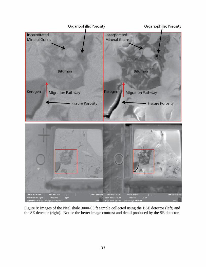
Figure 8 shows a comparison of BSE and SE images showing organic porosity development.

31

The organic porosity that developed with thermal maturation is much more visible in the SE

image, compared to the BSE image. However, it was found that by adjusting the threshold value

of the BSE detector to match the porosity imaged with the SE detector, the BSE detector also can

be used to analyze porosity development, which negates the image charging and shadowing

produced by the SE detector. Figure 9 shows the 3-D reconstruction completed for sample 3000-

05, and Table 2 shows the results of the analysis after the samples were reconstructed.

32

Figure 7: EDS maps of Neal shale 2920-25 ft sample, showing the location of organic matter

(blue arrow) and a pyrite framboid (red arrow). The scale bar shows 5 µm for all images.

33

Figure 8: Images of the Neal shale 3000-05 ft sample collected using the BSE detector (left) and

the SE detector (right). Notice the better image contrast and detail produced by the SE detector.

34

Figure 9: 3-D models of Neal shale 3000-05 ft sample from well 2191 showing the reconstructed

sample using A) the BSE detector, B) the SE detector, C) reconstructed organic matter, D)

porosity, and E) pyrite with the scale bar in micrometers.

35

Table 2: Results of FESEM 3-D reconstruction analysis of Neal shale samples, reported in

volume percent with porosity representing total porosity (- indicates samples where the BSE

detector was not used).

3.5 Modeling Results

3.5.1 Kinetic Porosity

The calculated kerogen porosity within the Neal shale ranges from 0.26– 4.82% and

averages 2.33% (Table 3). These values were calculated using Jarvie et al. (2007) alternative

methods to calculate input values for the Modica and Lapierre (2012) kinetic porosity model.

For Well 2191, with measured Ro values ranging from 0.92– 0.98%, calculated kerogen porosity

ranges from 0.26–1.15% and averages 0.62%. Well 1780 has measured Ro values ranging from

1.44– 1.59%; the calculated kerogen porosity ranges from 0.74– 4.82% and averages 2.40%.

Finally, for Well 15668 with Easy %Ro of 2.2– 2.3%, kerogen porosity ranges from 2.21– 4.63%

and averages 3.68%.

Depth Porosity Organic Matter Pyrite

2740-45 0.17 1.58 0.18

2830-35 1.12 3.80 0.63

2920-25 0.08 22.07 0.23

3000-05 0.43 5.90 0.42

6270-80 0.04 0.00 0.00

6370-80 7.74 0.00 0.09

6460-70 0.08 1.06 0.01

6560-70 0.01 3.71 1.06

9013.1 0.20 0.00 1.67

9022.8 0.12 8.95 -

9033.0 0.20 0.70 0.06

9044.0 0.01 0.00 -

9053.0 0.07 0.69 -

9062.7 1.56 0.00 0.00

9073.0 1.46 0.00 0.00

36

Table 3: Table of calculated kerogen porosity including input data.

3.5.2 Basin Modeling

Basin modeling of Well 2191 (Figure 10) was designed to correlate with the measured Ro

values from Carroll et al. (1995). By setting the amount of erosion to 7,300 ft and varying the

Top Depth (ft) HIo TRHI iTOC Cc PhiK

2740 439.25 0.49 1.94 0.24 0.55

2780 439.25 0.09 4.36 0.27 0.26

2820 439.25 0.68 2.55 0.28 1.15

2920 439.25 0.24 4.51 0.29 0.75

3010 439.25 0.95 0.61 0.27 0.37

6270 439.25 0.99 1.13 0.28 0.74

6300 439.25 0.96 1.35 0.28 0.86

6330 439.25 0.96 2.62 0.30 1.78

6340 439.25 0.93 2.74 0.30 1.82

6350 439.25 0.98 1.68 0.29 1.12

6360 439.25 0.98 1.56 0.28 1.03

6370 439.25 0.97 1.75 0.29 1.15

6380 439.25 0.97 1.50 0.28 0.98

6390 439.25 0.97 2.15 0.29 1.45

6410 439.25 0.97 2.22 0.29 1.50

6420 439.25 0.94 4.74 0.33 3.50

6430 439.25 0.95 3.69 0.31 2.61

6440 439.25 0.93 4.22 0.32 3.02

6450 439.25 0.94 4.23 0.32 3.04

6450 439.25 0.94 3.42 0.31 2.37

6460 439.25 0.93 5.17 0.34 3.82

6460 439.25 0.91 4.16 0.32 2.92

6470 439.25 0.93 4.12 0.32 2.91

6470 439.25 0.92 3.79 0.32 2.63

6480 439.25 0.91 5.80 0.35 4.32

6480 439.25 0.87 5.33 0.34 3.80

6490 439.25 0.96 6.15 0.34 4.82

6500 439.25 0.91 4.92 0.33 3.56

6510 439.25 0.92 2.83 0.30 1.88

6550 439.25 0.97 2.94 0.30 2.04

6560 439.25 0.97 3.78 0.31 2.74

9013.45 439.25 0.95 3.18 0.31 2.21

9016.75 439.25 0.97 5.90 0.34 4.63

9020.85 439.25 0.96 4.10 0.32 2.99

9023.05 439.25 0.95 5.56 0.34 4.24

9024.45 439.25 0.96 5.61 0.34 4.32

37

geothermal gradient through time, Easy %Ro values from Petromod® were 0.9– 1.0%, nearly

identical to the measured Ro values of 0.92– 0.98%.

Figure 10: Easy %Ro values for Well 2191.

Basin modeling of Well 1780 (Figure 11) was also designed to match measured Ro

values from Carroll et al. (1995). The same geothermal model was used for Well 1780 that was

used for Well 2191. Erosion was then set at 7,000 ft to match the measured Ro values of 1.44–

1.59%, producing Easy %Ro values of 1.5– 1.6% for Well 1780.

38

Figure 11: Easy %Ro values for Well 1780.

Basin modeling results from Well 15668 (Figure 12) were found by using the same

geothermal gradient and 7,000 ft of erosion. The Easy %Ro values range from 2.2– 2.3% within

the Neal shale, as compared to 1.26– 1.52% Ro values calculated from pyrolysis data.

39

Figure 12: Easy %Ro values for Well 15668.

A burial model for Well 2191 (Figure 13) shows the rapid burial that occurred due to the

Alleghanian Orogeny that began at the end of the Carboniferous and ended in the Late Permian.

This rapid burial forced the Neal shale in Well 2191 to a maximum depth of approximately

10,000 ft. Uplift then eroded approximately 7,300 ft of Pottsville sediment and brought the Neal

shale to much shallower depths. Overlaying Easy %Ro values shows that thermal maturation of

the kerogen occurred rapidly and correlates with the maximum depth of burial.

40

Figure 13: Burial history of Well 2191, including Easy %Ro values as an overlay.

A burial history model of Well 1780 (Figure 14) shows the rapid burial that began at the

end of the Carboniferous and continued through the Permian. Rapid burial forced the Neal shale

to a maximum depth of 12,500 ft and coincided with the timing of thermal maturation. Uplift

and an estimated 7,000 ft of Pottsville sediment erosion then brought the Neal shale to shallower

depths ranging from 6,000–6,270 ft.

41

Figure 14: Burial history of Well 1780, including Easy %Ro values as an overlay.

Modeling the burial history based on Well 15668 (Figure 15) also shows the deposition

of the Pottsville Formation that buried the Neal shale to a maximum depth of approximately

15,000 ft followed by 7,000 ft of erosion of the Pottsville Group. The timing of maximum burial

coincides with the maximum thermal maturity reached by the Neal shale and corresponds to a

Easy %Ro value of 2.2– 2.3%. Uplift and erosion placed the Neal shale at its current depth of

9,000–9,025 ft.

42

Figure 15: Burial history of Well 15668, including Easy %Ro values as an overlay.

The transformation ratio of the Neal shale (Figure 16) ranges from approximately 60%

within Well 2191, to 97% within Well 15668. The 60% transformation ratio places the Neal

shale in the early gas window for Well 2191, with hydrocarbon generation occurring rapidly

during the point of maximum burial. The 97% transformation ratio puts the Neal shale in the dry

gas window within both Well 1780 and Well 15668.

43

Figure 16: Transformation ratio of the kerogen within the Neal shale.

Figure 17 shows the burial history of Well 2191, including an overlay of the hydrocarbon

zones as determined by kinetic modeling. These zones indicate that the Neal shale rapidly

passed through the oil window and into the wet gas window during the time of maximum burial.

These zones are modeled by incorporating the HIo and the TOC of the sample and selecting the

kinetic parameters that best match the Neal shale. The kinetic models of hydrocarbon formation

in the Kimmeridge Clay were chosen to model the Neal shale because the two shales were

deposited in similar environments, are dominated by the same type of kerogen, and have similar

HIo values.

44

Figure 17: Burial history of Well 2191 with overlain hydrocarbon zones.

A burial model for Well 1780 (Figure 18) with hydrocarbon zone overlays shows the

Neal shale rapidly passed through the oil and wet gas window and into the dry gas window. This

timing corresponds to a maximum burial depth of approximately 10,000 ft during the Late

Permian. The formation has since been uplifted approximately 7,300 ft, whereupon kerogen

maturation rapidly ceased.

45

Figure 18: Burial history of Well 1780, with overlain hydrocarbon zones.

Modeling of Well 15668 (Figure 19) shows the Neal shale passed even further into the

dry gas window than in Well 1780. The Neal shale passed into the dry gas window beginning at

a burial depth of 14,000 ft, and was pushed even further into the dry gas window when buried to

the maximum depth of 15,000 ft.

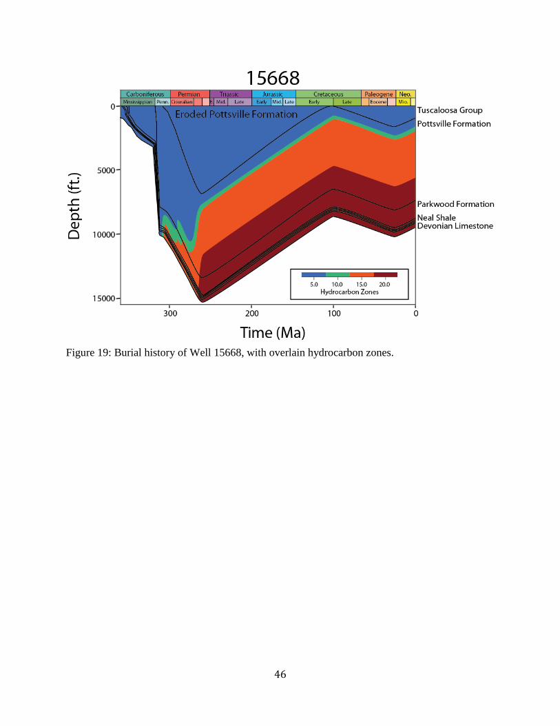
46

Figure 19: Burial history of Well 15668, with overlain hydrocarbon zones.

47

4 DISCUSSION

4.1 Mineralogy

XRD analysis results for Well 15668 samples were compared to those reported in the

Geological Survey of Alabama’s SEA shale study by ashin et al. (2011) for samples from

the same well. Mineralogical, tight rock, and Rock-Eval analyses were completed by TerraTek

for the RPSEA project. However, the TerraTek study reported illite/smectite and illite + mica as

combined values. As a result, it is difficult to compare the reported clay contents with those

determined by this study. The chlorite values differ by 7.9 wt% and the total wt% of clay varies

by 10 wt% for the 9013.1 ft sample analyzed by this study, compared to TerraTek’s® results for a

sample at 9013.2 feet. These differences in mineralogic composition likely come from the

different sampling depths. In both studies, the Neal shale was determined to be a clay-rich

formation.

An additional area of difference in XRD results is seen when the plagioclase

concentrations at 9,022.8 feet and 9,022.9 feet are compared. The largest difference is apparent

when the plagioclase content reported by TerraTek for a sample at 9,022.9 feet is compared to

that reported for albite by this study for a sample at 9,022.8 feet. The large difference of 7.7

wt% may be accounted for by the different sampling depths or through the use of different

plagioclase structures in the Rietveld analyses. This study used the structure for albite because it

provided the best fit to the XRD patterns, is the most common plagioclase, and is the most

resistant to weathering. These factors make it more likely to be incorporated in a shale formation

than anorthite. Despite these differences, the XRD results obtained in this study show good

overall agreement with those of Pashin et al. (2011).

48

A correlation matrix for the average mineralogical, elemental, and TOC contents (Figure

A-1) of the Neal shale samples selected for this study shows strontium concentrations correlate

to calcite and dolomite, as well as Mg and Ca. This relationship is likely due to Sr substitution

for Ca in CaCO3 which is a function of 1) the Sr/Ca ratio in the liquid phase from which the solid

phase is derived, 2) the temperature, and 3) the salinity of the liquid phase as described by

Turekian (1955). Sr/Ca ratios within the Neal shale range from 0.004 to 0.013 and average

0.006. Quartz is strongly correlated with the concentration of Si, with a correlation coefficient

(r) of 0.86, and moderately correlated to Zr with r =0.55, which is likely due to its association

with sediment shed from the same source. If not for the presence of silica within the structure of

clay minerals, it should be expected that this correlation would be near 1. The total wt% of the

clay minerals chlorite, illite, montmorillonite, and muscovite within the shale samples strongly

correlates with many of the trace elements. However, the strongest clay content correlation is to

Al, with r =0.93. Pyrite within the shale facies correlates with several trace element

concentrations, including V, Cr, Ni, Zn, and Ba, and also correlates with TOC. The genetic

relationship between TOC and pyrite formation is due to bacterially mediated sulfate reduction

during oxidation of organic matter, resulting in the production of hydrogen sulfide (Emeis and

Morse, 1990). Part of this reduced sulfur is then retained in iron sulfide minerals.

A distinction between the Neal shale and the Floyd Shale can be made based on

mineralogy and chemical composition. The Neal shale contains less quartz and more clay

minerals than the Floyd Shale, which is a mix of gray shale, limestone, and siltstone facies.

Because of this mineralogical difference, there is also a difference in the chemical compositions

of the shales. The Floyd Shale contains less Al2O3 due to the lower clay content. In addition,

because the Floyd Shale is richer in quartz, it has a higher SiO2 concentration. The Neal shale

49

also contains an average of 2.27 wt% TOC, while the Floyd Shale TOC is less than 0.5 wt%.

Because of the lower TOC content, the Floyd Shale has an average decrease of 47.2 percent in

the abundance of most trace elements.

The Neal shale sediment was transported towards the southeast along depositional strike

of the Warrior platform, and deposited in epeiric ramp and basinal environments during the Late

Mississippian. The formation is clay-rich, and quartz-poor with varying amounts of organic

matter. Zones where the quartz content is greater than 50 wt% may better represent the Floyd

Shale, which is a mixture of gray shale, limestone, and sandstone facies.

The Neal shale thins toward the southeast, where it interfingers with the Lewis

Limestone. The Well 15668 core contains 25 feet of the Neal shale facies and 48 ft of the

underlying Lewis Limestone. Within the Lewis Limestone is a 0.5 ft thick stringer of the Neal

shale. This was confirmed through XRD analysis in which the mineralogy of the stringer shale

was nearly identical to the thick section of Neal shale facies.

4.2 Strength Test

Uniaxial strength tests of selected Well 15668 core samples show that the Neal shale has

a lower strength than the underlying Lewis Limestone. This suggests that the Lewis Limestone

may serve as an active barrier during hydraulic fracturing of the Neal shale, if horizontal wells

are used. Hydraulic fracturing of the Barnett Shale within the Fort Worth Basin is more

successful where the quartz content is greater than 45 wt% and the clay content is less than 27

wt% (Bowker, 2003). This statement could not be tested within the Neal shale due to the lack of

equipment available to accurately measure the maximum load required for failure. However, an

overall comparison of the Neal shale strength to the Lewis Limestone strength shows that

mineralogy plays an important role in fracturing success.

50

Axial tests of the Neal shale indicate that it has a higher strength than in diametral tests,

for unconfined samples collected at the same depth. This occurs because the formation is highly

friable and breaks along pre-existing planes of weakness due to bedding. At reservoir

conditions, the Neal shale would not fracture along these planes of weakness, but would cut

perpendicularly across them. Axial strength results would thus provide more accurate results

when designing the fracture stimulation job. One major factor that could not be tested was the

strength of the Neal shale at the confining pressure of the surrounding rock. At reservoir

conditions, the Neal shale will not have the same strength as indicated by unconfined

compressive strength tests. Strength tests should be conducted at a variety of confining pressures

to enable extrapolation to reservoir conditions. Strength tests at reservoir conditions were

beyond the scope of this project and the equipment necessary to conduct such tests was not

available.

4.3 Organic Porosity

The Neal shale was rapidly buried during the Permian, followed by rapid uplift and

subsequent erosion of the overlying Pottsville sediments. During the time of maximum burial,

the Neal shale was pushed through the oil window and into the wet-dry gas windows. It was at

this time that a large volume of hydrocarbons were generated and expelled into overlying

reservoirs. In addition to the large volume of hydrocarbons expelled from the formation, the

Neal shale also retained a substantial volume of hydrocarbons both within its pore spaces and

adsorbed onto organic material. The basin model indicates that further burial during the

Cretaceous-Paleogene did not result in further maturation of the kerogen or petroleum

generation. The Neal shale is modeled to contain condensate within the less mature Well 2191,

51

while dry gas dominates in the more mature Wells 1780 and 15668. The average TOC used for

this analysis was 2.27 wt%, based on the correlation of XRF Cr+Ni+Mo concentrations with

TOC data obtained by pyrolysis (Pashin et al., 2011). Also, the Langmuir pressure and volume

determined by the Pashin et al. (2011) study were incorporated in the basin model to determine

the adsorbed volume of hydrocarbons.

Figure 8 shows that there are two distinctly different types of porosity present within the

Neal shale organic matter. The first type is fissure porosity, which may be the result of oil

generation, as proposed by Curtis et al. (2013). The fissure porosity is only present in the

organic material at the lower left, and ends at the juncture with the more circular patch of organic

matter. Curtis et al. (2013) suggested that with oil generation and pressure build up, oil may

hydraulically fracture the organic matter. Oil generation may therefore be the cause of the

fissure porosity seen within the organic matter of the Neal shale. The second porosity type is

organophillic porosity, in which round pores have developed from the generation of gas.

Organophillic porosity is only evidenced within the adjacent circular patch of organic material.

The interpretation for the organic material shown in Figure 8 is that the irregular patch of organic

material in the lower left of the image is kerogen, and the circular patch of organic material is

bitumen or pyrobitumen. As the kerogen broke down to form oil, overpressuring occurred,

creating the kerogen fissure porosity and allowing the migration of petroleum. In this sample,

the petroleum did not migrate far before organophillic porosity developed. The other

distinguishing characteristic between these two patches of organic material is that the circular

patch shows entrained inorganic mineral grains, which likely formed during the fracturing

process.

52

Kerogen within the Neal shale has been reported by Carroll et al. (1995) to be dominated

by matrix bituminite (95%), with minor accumulations of liptinite (1%), vitrinite (3%), and

inertinite (1%). Using these kerogen maceral concentrations and equation (1), the HIo value

calculated in the current study for the Neal shale is 439.25. This value was compared to the HI

values calculated by Pashin et al. (2011) for the least mature Well 2191, in which the highest HI

value was 427. This similarity suggests that the calculated HIo value of 439.25 is reasonable.

The hypothesis of this study was that as kerogen breaks down to form hydrocarbons,

porosity ensues. Results from the Modica and Lapierre (2012) kinetic model of porosity

development indicate that kerogen within the Neal shale has developed as much as 4.82%

porosity. However, this value does not agree with FIB-FESEM observations of kerogen porosity

within the Neal shale. The maximum organic porosity found in this study was 1.12% at a sample

depth of 2,830 ft, and organic matter interpreted to be kerogen was not observed to develop any

organophillic porosity. While the maximum observed organic porosity value is nearly identical

to the kinetic model calculation of 1.15% kerogen porosity at sample depth 2,820 ft, at all other

sample depths porosity is highly overestimated by the kinetic model. One possible explanation

for this discrepancy is that the FESEM cannot resolve pore spaces smaller than a few

nanometers. This would lead to the method underestimating the porosity within both organic

matter and the inorganic matrix, if it is in the sub-nanometer size range. Another explanation for

the difference in calculated and observed porosity development may be that kerogen does not

break down with thermal maturation to form porosity, as originally hypothesized. If the

interpretation of Figure 2 is correct, then it is not the kerogen that breaks down to form

organophillic porosity, as modeled by Modica and Lapierre (2012), but rather bitumen or

pyrobitumen. This indicates that thermal maturity is not the only driving force for porosity

53

development, and suggests that the chemical makeup of the organic material is also a primary

control. This conclusion agrees with previous studies of shale porosity development in which

samples at the same thermal maturity level were observed to have different kerogen porosity

values (Curtis et al., 2011, 2012). To accurately model organic porosity development, the

volumes of bitumen or pyrobitumen retained during maturation and the degree of compaction

during subsequent burial need to be known. In addition, organic fracturing caused by oil

generation should be investigated further as a source of porosity.

4.4 Volumetric Analysis

The Neal shale has a large potential to store hydrocarbons. Porosity values within the

formation range from 2.4– 7.7%, while hydrocarbon saturation values range from 29.9– 78.8%,

based on TerraTek® TRA (Pashin et al., 2011). Rose and Associates risk analysis performed

using this data, and the results of basin modeling, were used to calculate the volume of

recoverable free gas and adsorbed gas in place (table 4).

Table 4: Recoverable free gas estimates and adsorbed gas-in-place based on risk analysis and

basin modeling.

Free Gas

Area (km²) Oil (MMbo) Gas (Bcf)

P90 6690 0.01 227.22

P10 6690 12.89 4943.27

Adsorbed Gas

Well Area (km²) (Mcf/km²) Mcf Tcf

2191 2230 179915.10 401210673.00 401.21

1780 2230 19559.71 43618153.30 43.62

15668 2230 6902.39 15392329.70 15.39

Total 6690 - 460221156.00 460.22

54

The Neal shale of Alabama has a large resource potential. Based on Rose and Associates

risk analysis, there is a 10% chance that 4.94 Tcf and a 90% chance that 227.22 Bcf may be

recovered from the free space of the formation. Because the formation is within the wet gas

window for Well 2191, it has been estimated that the oil concentration may range from 0–5%, at

most. If this were the case, there would be a 10% chance that 12.89 MMbo are recoverable from

the formation and a 90% chance that 0.01 MMbo are recoverable. The estimated volume of

recoverable free gas from the Neal shale is minor compared to the volume of adsorbed gas within

the formation. As the temperature of the formation decreases, Zhou et al. (2000) showed that the

ability of methane to adsorb on activated carbon increases. The molecular sizes of the

hydrocarbon components present within the formation also play a role in determining adsorption

affinities and thus the overall volume of gas adsorbed to the organic material (Jarvie et al., 2007).

Pepper (1992) estimated that gas adsorption may be reduced by a factor of 10 at high maturities.

For example, as the source rock passes from the oil window to the gas window, adsorption of

higher molecular weight hydrocarbons decreases from approximately 200 mg HC/g TOC to 20

mg HC/g TOC. An average TOC value of 2.27 wt% was used to determine the volume of gas

adsorbed within the Neal shale. At a temperature of approximately 150°F, Easy %Ro of 2.1–

2.2% and lithostatic pressure of 62– 63 MPa, the Neal shale adsorbs 6,902.39 Mcf/km2. Gas

adsorption on the Neal shale increases dramatically at lower temperatures and maturities as seen

in the adsorption model of Well 2191 (Table 4). The bottom-hole temperature for Well 2191 is

approximately 100°F, while lithostatic pressure ranges from 19.5– 21 Mpa. Gas adsorption may

be as great as 179,918 Mcf/km2 within this well, where condensate is also modeled to occur.

55

5 CONCLUSIONS

The Neal shale of Alabama is a clay-rich, quartz-poor formation, with TOC contents

averaging 2.27 wt%. TOC values can be estimated for samples where pyrolysis data are lacking,

using a linear equation derived from the correlation between the sum of trace element

concentrations (Cr+Mo+Ni) and measured TOC values.

Porosity within the Neal shale is a mix of fissure, organophillic, and intergranular

porosity. Kinetic models of porosity development indicate that organic matter within the Neal

shale may have developed as much as 4.5% porosity, while FIB-FESEM results show a

maximum of 1.12% porosity development. In addition, there is no evidence for an increase in

organic porosity with increasing thermal maturation, based on FIB-FESEM imaging. Organic

porosity development within the Neal shale is a mixture of fissure and organophillic porosity.

Fissure porosity is likely related to the generation of oil from kerogen creating overpressuring

and fracturing. With additional maturation, this was followed by gas generation which created

organophillic porosity within bitumen.

Basin modeling shows the Neal shale was rapidly buried during the Mississippian,

resulting in kerogen maturation and hydrocarbon generation. Burial was followed by uplift and

erosion of the overlying Pottsville sediments from the Early Permian to the Early Cretaceous,

which brought the formation to much shallower depths. During the time of maximum burial, the

Neal shale generated a large volume of hydrocarbons. Up to 460 Tcf of gas may be adsorbed

onto the organic matter of the formation, while free gas estimates range from 227–4,493 Bcf.

The underlying Lewis Limestone has an average unconfined diametral strength of 22.22 MPa

and should serve as an active barrier to hydraulic fracturing efforts in the Neal shale, which has

an average unconfined axial strength of 3.19 MPa

56

REFERENCES

Ambrose, R. J., Hartman, R. C., Diaz-Campos, M., Akkutlu, I. Y., & Sondergeld, C. H., 2012,

Shale gas-in-place calculations part I: New pore-scale considerations. SPE Journal 17(01),

219-229.

ASTM Standard D7012-13, 2013, Standard test methods for compressive strength and elastic

moduli of intact rock core specimens under varying states of stress and temperature, ASTM

International, West Conshohocken, PA, 2013, DOI: 10.1520/D7012, www.astm.org.

Bernard, S., Wirth, R., Schreiber, A., Schulz, H., & Horsfield, B., 2012, Formation of

nanoporous pyrobitumen residues during maturation of the Barnett Shale (Fort Worth

Basin). International Journal of Coal Geology 103, 3-11.

Bowker, K. A., 2003, Recent development of the Barnett Shale play. Fort Worth Basin: West

Texas Geological Society Bulletin 42(6), 4-11.

Carroll, R. E., Pashin, J. C., & Kugler, R. L., 1995, Burial history and source-rock characteristics

of Upper Devonian through Pennsylvanian strata, Black Warrior Basin, Alabama: Alabama

Geological Survey Circular 187, 29 p.

Cleaves, A. W., & Broussard, M. C., 1980, Chester and Pottsville depositional systems, outcrop

and subsurface, in the Black Warrior Basin of Mississippi and Alabama: Gulf Coast

Association of Geological Societies Transactions, Vol. 30, p. 49-60.

Curtis, M. E., Ambrose, R. J, Sondergeld, C. S., & Rai, C. S., 2010, Structural characterization of

gas shales on the micro- and nano-scales. SPE-137693, paper presented at the CSUG/SPE

Canadian Unconventional Resources and International Petroleum Conference, Calgary,

Alberta, October 19-21, 2010.

Curtis, M. E., Ambrose, R. J., Sondergeld, C. H., & Rai, C. S., 2011, Investigation of the

relationship between organic porosity and thermal maturity in the Marcellus shale. SPE-

144370, SPE Unconventional Gas Conference and Exhibition, June 12-16, 2011, The

Woodlands, Texas.

Curtis, M. E., Cardott, B. J., Sondergeld, C. H., & Rai, C. S., 2012, Development of organic

porosity in the Woodford Shale with increasing thermal maturity. International Journal of

Coal Geology Vol. 103, p. 26-31.

Curtis, M. E., Sondergeld, C. H., & Rai, C. S., 2013, Relationship between organic shale

microstructure and hydrocarbon generation. Society of Petroleum Engineers.

Doi:10.2118/164540-MS.

DIFFRACplus TOPAS R Version 3.0 Tutorial, 2005. Bruker D8 Advance Diffractometer.:

BRUKER AXS, INC., Madison, WI.

57

Emeis, K. C. and Morse, J. W., 1990, Organic carbon, reduced sulfur, and iron relationships in

sediments of the Peru Margin, sites 680 and 688. Proceedings of the Ocean Drilling

Program, Scientific Results, Vol. 112, p. 441-453.

Goldstein, J., Newbury, D. E., Joy, D. C., Lyman, C. E., Echlin, P., Lifshin, E., Sawyer, L., and

Michael, J. R., 2003, Scanning electron microscopy and X-ray microanalysis, 3rd edition,

Springer, New York, NY. 690 p.

Groshong, R. H., Jr., Hawkins, W. B*, Jr., Pashin, J. C., and Harry, D. L., 2010, Extensional

structures of the Alabama promontory and Black Warrior foreland basin: Styles and

relationship to the Appalachian fold-thrust belt, in Tollo, R.P., Bartholomew, M.J., Hibbard,

J. P., and Karabinos, P. M., eds., From Rodinia to Pangea: The Lithotectonic Record of the

Appalachian Region: Geological Society of America Memoir 206, p. 579-605.

Hatch, J. R., & Pawlewicz, M. J., 2007, Introduction to the assessment of undiscovered oil and

gas resources of the Black Warrior Basin province of Alabama and Mississippi, in Hatch,

Joseph R., and Pawlewicz, M. J., compilers, Geologic assessment of undiscovered oil and

gas resources of the Black Warrior Basin Province, Alabama and Mississippi: U.S.

Geological Survey Digital Data Series DDS–69–I, chap. 2, 6 p.

Jarvie, D. M., Hill, R. J., Ruble, T. E., & Pollastro, R. M., 2007, Unconventional shale-gas

systems: The Mississippian Barnett Shale of north-central Texas as one model for

thermogenic shale-gas assessment. AAPG Bulletin 91(4), 475-499.

Lopatin, N. V., 1971, Temperature and time as geologic factors in coalification (in Russian): Izv.

Akad. Nauk SSSR, Seriya Geologicheskaya, (3), 95-106.

McCarthy, K., Rojas, K., Niemann, M., Palmowski, D., Peters, K., & Stankiewicz, A., 2011,

Basic petroleum geochemistry for source rock evaluation. Oilfield Review 23(2), 32-43.

Modica, C. J. and Lapierre, S. G., 2012, Estimation of kerogen porosity in source rocks as a

function of thermal transformation: Example from the Mowry Shale in the Powder River

Basin of Wyoming. AAPG Bulletin 96(1), 87-108.

Okiongbo, K. S., Aplin, A. C., & Larter, S. R., 2005, Changes in type II kerogen density as a

function of maturity: Evidence from the Kimmeridge Clay formation. Energy & Fuels

19(6), 2495-2499.

Pashin, J. C., 1994, Cycles and stacking patterns in Carboniferous rocks of the Black Warrior

foreland basin: Gulf Coast Association of Geological Societies Transactions, v. 44, p. 555-

563.

Pashin, J. C. and Raymond, D. E., Glacial-eustatic control of coalbed methane reservoir

distribution (Pottsville Formation; Lower Pennsylvanian) in the Black Warrior Basin of

Alabama, 2004 Interntational Coalbed Methane Symp. Proc., Univ. Alabama, Tuscaloosa,

paper 413 (2004) 15 p.

58

Pashin, J. C., 2008 Gas shale potential of Alabama: Tuscaloosa, Alabama, University of

Alabama, College of Continuing Studies, 2008 International Coalbed & Shale Gas

Symposium Proceedings, paper 0808, 13 p.

Pashin, J. C., Kopaska-Merkel, D. C., Arnold, A. C., and McIntyre, M. R., 2011, Geological

foundation for production of natural gas from diverse shale formations: Sugarland, Texas,

Research Partnership to Secure Energy for America (RPSEA) Final Report, 7122.17.01;

Geological Survey of Alabama Open-File Report 1110, 156 p.

Pawlewicz, M. J., & Hatch, J. R., 2007, Petroleum assessment of the Chattanooga Shale/Floyd

Shale–Paleozoic total petroleum system, Black Warrior Basin, Alabama and Mississippi, in

Hatch, Joseph R., and Pawlewicz, Mark J., compilers, Geologic assessment of undiscovered

oil and gas resources of the Black Warrior Basin Province, Alabama and Mississippi: U.S.

Geological Survey Digital Data Series DDS-69-I, chap. 3, p. 1-23.

Pelet, R., 1985, Quantitative evaluation of products formed during the geochemical evolution of

organic matter, v. 40, no. 5, p. 551-562

Pepper, A. S., 1992, Estimating the petroleum expulsion behavior of source rocks: A novel

quantitative approach, in W. A. England and A. L. Fleet, eds., Petroleum migration:

Geological Society (London) Special Publication 59, p. 9-31.

Pepper, A. S., and Corvie, P. J., 1995, Simple kinetic models of petroleum formation. Part I: oil

and gas generation from kerogen. Marine and Petroleum Geology, 12(3), p. 291-319.

PetroMod: Petroleum systems modeling software (v2012.2 Windows 64-bit) [software]. (2011):

Schlumberger.

Rietveld, H.M., 1969, A profile refinement method for nuclear and magnetic structures. Journal

of Applied Crystallography, 2 (2): p. 65-61. doi:10.1107/S0021889869006558

Rose & Associates Multi-Method Risk Analysis (v4-4-051) [software]. (2012). Rose &

Associates, LLP.

Sondergeld, C. H., Ambrose, R. J., Rai, C. S., & Moncrieff, J., 2010, Micro-structural studies of

gas shales. SPE-131771, SPE Unvonventional Gas Conference, Pittsburgh, PA, February

23-25, 2010.

Sweeney, J. J. and Burnham, A. K., 1990, Evaluation of a simple model of vitrinite reflectance

based on chemical kinetics. American Association of Petroleum Geologists Bulletin, 74,

p. 1559-1570.

Telle, W. R., Thompson, D. A., Lottman, L. K., and Malone, P. G., 1987, Preliminary burial-

thermal history investigations of the Black Warrior basin: implications for coalbed methane

and conventional hydrocarbon development: Tuscaloosa, Alabama, University of Alabama,

1987 Coalbed Methane Symposium Proceedings, p. 37-50.

59

Thomas, W. A., 1977, Evolution of Appalachian-Ouachita salients and recesses from reentrants

and promontories in the continental margin. American Journal of Science 277 (10), p. 1233-

1278.

Thomas, W. A., 1988, The Black Warrior Basin, in Sloss, L. L., ed., Sedimentary cover–North

American craton: Geological Society of America, The Geology of North America, v. D-2, p.

471-492.

Turekian, K., 1955, Paleoecological significance of the strontium-calcium ratio in fossils and

sediments. Geological Society of America Bulletin, 66 (1), p. 155-158.

Zhou, L., Zhou, Y., Li, M., Chen, P., & Wang, Y., 2000, Experimental and modeling study of the

adsorption of supercritical methane on a high surface activated carbon. Langmuir, 16(14), p.

5955-5959.

APPENDIX

60

Table A-1: Geochemical data for the Neal shale (from Pashin et al., 2011).

Top TOC

Depth (ft) (wt%)

2191 2740 Neal 1.71 0.88 4.78 0.34 442 280 20

2191 2780 Neal 4.25 2.52 18.16 0.54 440 427 13

2191 2820 Neal 2.07 0.72 3.97 0.29 441 192 14

2191 2920 Neal 4.19 1.65 15.67 0.49 441 374 12

2191 3010 Floyd 0.46 0.02 0.16 0.3 478 35 65

1780 6270 Neal 0.82 0.05 0.06 0.15 454 7 18

1780 6300 Neal 0.99 0.07 0.27 0.1 465 27 10

1780 6330 Neal 1.87 0.23 0.56 0.29 448 30 16

1780 6340 Neal 1.97 0.45 0.98 0.27 451 50 14

1780 6350 Neal 1.21 0.06 0.17 0.15 451 14 12

1780 6360 Neal 1.13 0.06 0.19 0.1 467 17 9

1780 6370 Neal 1.26 0.06 0.24 0.12 467 19 10

1780 6380 Neal 1.09 0.07 0.23 0.12 468 21 11

1780 6390 Neal 1.54 0.09 0.31 0.07 454 20 5

1780 6410 Neal 1.59 0.12 0.35 0.14 456 22 9

1780 6420 Neal 3.27 0.53 1.28 0.26 454 39 8

1780 6430 Neal 2.59 0.34 0.91 0.12 453 35 5

1780 6440 Neal 2.95 0.67 1.42 0.2 456 48 7

1780 6450 Neal 2.95 0.45 1.21 0.17 457 41 6

1780 6450 Neal 2.42 0.47 1.05 0.28 452 43 12

1780 6460 Neal 3.56 0.58 1.7 0.17 454 48 5

1780 6460 Neal 2.93 0.79 1.72 0.27 455 59 9

1780 6470 Neal 2.89 0.47 1.37 0.13 451 47 4

1780 6470 Neal 2.69 0.62 1.51 0.2 461 56 7

1780 6480 Neal 3.98 0.9 2.44 0.24 456 61 6

1780 6480 Neal 3.73 1.28 3.06 0.29 458 82 8

1780 6490 Neal 4.12 0.29 1.2 0.48 453 29 12

1780 6500 Neal 3.42 0.72 1.94 0.21 458 57 6

1780 6510 Neal 2.04 0.45 1.08 0.07 458 53 3

1780 6550 Neal 2.08 0.08 0.45 0.17 453 22 8

1780 6560 Neal 2.63 0.1 0.49 0.41 436 19 16

15668 9013.45 Neal 2.25 0.21 0.70 0.99 482 31 44

15668 9016.75 Neal 3.96 0.13 0.82 0.40 475 21 10

15668 9020.85 Neal 2.84 0.15 0.69 0.16 468 24 6

15668 9023.05 Neal 3.78 0.25 1.24 0.26 477 33 7

15668 9024.45 Neal 3.80 0.26 1.08 0.15 469 28 4

S3 (mg/g) Tmax(oC) HI OIPermit Formation S1(mg/g) S2 (mg/g)

APPENDIX

61

Table A-2: XRD results for Well 2191 samples.

Dep

th (

ft)

Fo

rmat

ion

Qu

artz

Alb

ite

Cal

cite

Ch

lori

te

Do

lom

ite

Flu

ori

te

Illi

te

Mo

ntm

ori

llo

nit

e

Mu

sco

vit

e

K-s

par

Py

rite

Su

m C

lay

2740-45 Neal 34.2 4.3 21.3 6.0 6.9 0.0 0.0 3.3 10.7 12.1 1.1 20.0

2750-55 Neal 22.2 2.2 14.7 6.1 10.0 1.2 26.4 0.7 6.9 8.5 1.2 40.0

2760-65 Neal 18.7 4.4 9.5 6.9 16.3 0.0 0.0 0.3 28.0 14.6 1.3 35.2

2770-75 Neal 26.2 3.0 18.3 12.1 9.4 0.0 17.3 0.0 2.5 9.5 1.6 31.9

2780-85 Neal 29.0 3.1 9.8 9.2 3.8 0.2 28.1 0.8 3.7 9.7 2.5 41.7

2790-95 Neal 27.1 3.9 8.2 7.9 2.2 0.5 31.2 0.6 6.7 9.8 1.9 46.3

2800-05 Neal 25.7 2.9 10.7 9.6 2.6 0.0 28.9 0.1 6.4 10.9 2.2 45.1

2810-15 Neal 34.0 7.5 1.5 14.5 1.0 0.0 0.0 0.5 28.9 11.9 0.2 43.9

2820-25 Neal 27.4 3.4 1.7 9.4 1.5 0.0 32.8 2.7 10.4 8.3 2.3 55.3

2830-35 Neal 21.9 4.2 2.6 9.0 2.1 1.0 31.2 4.5 9.7 12.6 1.1 54.4

2840-45 Neal 37.0 1.6 6.0 6.5 1.0 0.0 25.1 1.2 6.7 14.0 1.0 39.5

2850-55 Neal 16.7 7.8 6.9 8.2 3.3 0.0 0.0 1.7 25.6 28.6 1.2 35.5

2860-65 Neal 26.8 4.3 10.2 5.3 3.3 1.7 28.2 1.3 6.1 11.4 1.4 40.9

2870-75 Neal 25.3 4.5 13.8 5.9 3.1 0.0 26.8 0.4 6.7 11.9 1.6 39.8

2880-85 Neal 20.0 3.6 7.4 5.5 1.9 1.5 34.6 2.2 11.5 10.6 1.1 53.8

2890-95 Neal 18.6 1.8 12.7 8.4 3.4 3.8 27.7 0.4 13.1 9.6 0.6 49.6

2900-05 Neal 21.4 2.1 7.6 10.7 2.3 2.4 30.8 0.5 9.6 11.3 1.2 51.7

2910-15 Neal 20.3 1.2 15.2 9.7 1.9 0.4 30.0 1.1 9.8 8.6 1.8 50.5

2920-25 Neal 23.3 2.8 9.9 8.0 1.4 2.6 30.7 1.3 7.6 10.6 1.8 47.6

2930-35 Neal 17.7 3.1 15.9 4.4 18.1 0.0 0.0 0.0 27.6 12.5 0.7 31.9

2940-45 Neal 23.4 4.1 15.3 5.3 4.1 0.0 0.0 0.7 26.1 20.2 0.7 32.1

2950-55 Floyd 51.4 0.0 19.3 7.3 5.7 0.0 0.0 0.5 3.5 11.4 0.9 11.4

2960-65 Floyd 50.1 2.6 1.6 4.3 1.7 0.0 14.1 1.9 11.4 11.9 0.4 31.7

2970-75 Floyd 59.1 2.6 1.1 4.8 0.9 0.3 9.7 1.6 8.4 11.0 0.6 24.4

2980-85 Floyd 69.5 2.2 1.5 7.4 1.0 0.0 0.0 1.5 5.3 11.1 0.5 14.2

2990-95 Floyd 69.5 2.5 1.5 6.2 0.8 0.0 0.0 1.4 6.5 11.2 0.4 14.1

3000-05 Floyd 51.5 1.6 21.2 5.5 5.5 0.0 0.0 1.1 3.7 9.2 0.5 10.4

APPENDIX

62

Table A-3: XRD results for Well 1780 samples.

Dep

th (

ft)

Fo

rmat

ion

Qu

artz

Alb

ite

Cal

cite

Ch

lori

te

Do

lom

ite

Flu

ori

te

Illi

te

Mo

ntm

ori

llo

nit

e

Mu

sco

vit

e

K-s

par

Py

rite

Sid

erit

e

Su

m C

lay

6270-80 Neal 23.3 3.3 22.2 8.2 5.0 0.1 25.4 1.2 5.6 5.3 0.5 0.0 40.4

6280-90 Neal 18.8 4.8 36.2 9.3 4.3 0.0 0.0 0.7 18.8 6.2 0.8 0.0 28.9

6290-00 Neal 14.7 9.8 5.7 11.9 0.8 0.0 0.0 0.1 38.0 18.6 0.4 0.0 50.0

6300-10 Neal 23.3 5.5 6.0 7.4 3.3 0.0 22.2 0.0 22.3 9.7 0.3 0.0 51.9

6310-20 Neal 23.3 3.6 22.4 8.7 7.6 0.9 23.9 0.5 3.8 5.0 0.4 0.0 36.9

6320-30 Neal 23.2 3.4 13.3 8.5 9.8 2.7 29.0 0.5 2.6 6.6 0.4 0.0 40.5

6330-40 Neal 33.0 3.0 13.8 14.4 9.9 0.0 16.3 0.0 4.9 3.2 1.5 0.0 35.6

6340-50 Neal 21.8 8.4 8.3 9.2 7.1 0.0 0.0 0.2 28.6 14.8 1.7 0.0 37.9

6350-60 Neal 25.3 3.9 9.8 9.5 6.9 0.4 26.7 1.2 5.6 9.4 1.4 0.0 42.9

6360-70 Neal 19.3 7.1 3.0 12.7 1.2 0.0 26.8 1.1 3.3 25.1 0.5 0.0 43.9

6370-80 Neal 28.6 3.6 2.6 11.7 1.4 0.0 24.9 0.1 15.9 10.8 0.3 0.0 52.7

6380-90 Neal 30.2 2.7 5.4 11.6 1.5 0.0 33.8 1.6 4.4 8.1 0.7 0.0 51.4

6390-00 Neal 25.4 1.7 0.4 12.6 0.4 2.3 36.2 0.5 10.2 9.4 0.9 0.0 59.5

6400-10 Neal 22.3 3.8 1.4 10.7 1.7 3.4 31.1 0.4 12.6 11.9 0.6 0.0 54.9

6410-20 Neal 23.1 3.4 3.0 9.9 3.2 2.3 32.0 2.4 10.2 9.9 0.6 0.0 54.5

6420-30 Neal 30.5 4.8 2.1 8.1 6.1 1.1 30.1 1.5 4.0 10.8 1.0 0.0 43.7

6430-40 Neal 15.3 7.4 2.0 8.2 6.2 0.0 13.1 13.6 5.2 28.2 0.9 0.0 40.1

6440-50 Neal 32.7 5.5 0.0 9.2 4.4 0.0 28.0 0.1 6.9 12.1 1.2 0.0 44.2

6450-60 Neal 27.8 4.4 3.1 9.2 5.8 0.7 32.0 0.3 7.3 7.8 1.6 0.0 48.9

6460-70 Neal 28.8 5.9 1.1 8.8 7.6 0.6 32.3 0.7 3.4 8.6 2.2 0.0 45.2

6470-80 Neal 25.5 4.4 1.9 10.1 4.8 2.4 37.0 0.4 3.5 8.7 1.2 0.0 51.0

6480-90 Neal 25.9 5.4 0.8 9.7 3.8 1.3 36.5 0.6 6.2 8.3 1.4 0.0 53.1

6490-00 Neal 25.5 5.5 9.0 7.4 4.5 0.0 30.4 0.7 5.5 9.7 1.8 0.0 44.0

6500-10 Neal 28.4 4.2 5.1 11.2 5.0 2.3 30.9 0.4 4.0 6.8 1.7 0.0 46.5

6510-20 Neal 25.4 3.2 18.9 7.7 4.3 0.0 21.1 0.3 8.1 10.0 1.0 0.0 37.2

6520-30 Neal 16.1 4.9 30.9 2.6 7.0 0.0 0.0 11.2 13.2 13.5 0.6 0.0 27.0

6530-40 Neal 35.0 2.1 35.4 5.8 5.4 0.0 0.0 1.9 7.4 6.7 0.5 0.0 15.0

6540-50 Neal 25.5 2.8 15.2 6.4 5.5 2.5 24.6 2.2 6.7 8.2 0.7 0.0 39.8

6550-60 Neal 27.6 3.0 11.8 7.1 5.3 1.8 27.4 1.3 5.0 8.9 0.7 0.0 40.8

6560-70 Neal 28.8 4.3 14.3 7.9 2.3 1.0 22.7 0.9 7.1 7.5 0.6 2.6 38.6

APPENDIX

63

Table A-4: XRD results for Well 15668 samples.

Dep

th (

ft)

Fo

rmat

ion

Qu

artz

Alb

ite

Cal

cite

Ch

lori

te

Do

lom

ite

Flu

ori

te

Illi

te

Mo

ntm

ori

llo

nit

e

Mu

sco

vit

e

K-s

par

Py

rite

Su

m C

lay

9013.1 Neal 32.3 3.0 0.0 7.9 7.4 0.0 32.1 0.6 5.5 8.8 2.4 46.1

9022.8 Neal 37.0 8.7 0.0 7.8 6.0 0.0 23.1 0.2 2.7 12.3 2.2 33.8

9033.0 Lewis 9.5 6.8 46.6 2.7 18.7 0.0 0.0 1.8 12.3 1.0 0.7 16.7

9044.0 Lewis 1.6 2.0 88.4 4.8 2.7 0.0 0.0 0.1 0.0 0.0 0.5 4.8

9053.0 Neal 17.8 6.0 2.0 7.5 7.4 4.0 31.5 0.0 11.2 11.8 0.8 50.2

9062.7 Lewis 10.8 2.0 79.2 3.8 1.2 0.0 0.0 0.0 2.7 0.0 0.3 6.4

9073.0 Lewis 72.4 1.7 15.2 2.3 2.3 0.0 0.0 2.5 0.0 3.5 0.2 4.8

APPENDIX

64

Table A-5: XRF results for Well 2191 samples.

(σ denotes standard deviation)

Depth (ft) SiO2 TiO2 Al2O3 Fe2O3 MnO MgO CaO Na2O K2O P2O5

2740-45 63.929 0.543 10.575 3.918 0.030 1.748 16.488 0.538 1.918 0.131

σ 0.053 0.002 0.023 0.003 0.000 0.004 0.009 0.003 0.001 0.001

2750-55 59.049 0.683 15.139 5.897 0.048 2.349 13.194 0.681 2.551 0.209

σ 0.051 0.001 0.029 0.006 0.000 0.010 0.013 0.007 0.005 0.001

2760-65 57.327 0.734 15.854 5.825 0.055 3.187 13.215 0.706 2.723 0.176

σ 0.054 0.001 0.021 0.002 0.000 0.009 0.012 0.003 0.006 0.000

2770-75 57.767 0.714 15.077 5.876 0.043 2.403 14.176 0.713 2.768 0.235

σ 0.011 0.002 0.010 0.004 0.000 0.004 0.005 0.003 0.003 0.001

2780-85 62.089 0.778 16.812 6.548 0.033 2.033 7.500 0.750 2.999 0.215

σ 0.059 0.003 0.015 0.002 0.000 0.004 0.005 0.005 0.007 0.001

2790-95 63.007 0.874 17.850 5.999 0.032 1.964 5.931 0.778 3.163 0.160

σ 0.062 0.002 0.026 0.002 0.000 0.005 0.009 0.004 0.006 0.000

2800-05 60.747 0.842 18.344 6.657 0.033 2.120 6.949 0.834 3.059 0.180

σ 0.125 0.002 0.047 0.005 0.000 0.011 0.008 0.005 0.006 0.001

2810-15 64.975 0.835 20.393 5.816 0.023 1.987 1.857 0.938 2.904 0.111

σ 0.312 0.001 0.086 0.007 0.000 0.006 0.004 0.005 0.007 0.001

2820-25 63.791 0.794 19.727 6.848 0.037 2.017 2.747 0.879 2.875 0.121

σ 0.097 0.002 0.043 0.007 0.000 0.003 0.003 0.006 0.004 0.001

2830-35 64.727 0.817 19.733 5.671 0.029 1.930 3.025 0.888 2.885 0.125

σ 0.050 0.004 0.018 0.004 0.000 0.005 0.005 0.007 0.005 0.000

2840-45 64.998 0.797 17.934 5.829 0.029 1.785 4.838 0.810 2.666 0.152

σ 0.034 0.002 0.008 0.004 0.000 0.005 0.004 0.003 0.006 0.000

2850-55 62.951 0.797 16.641 5.580 0.033 1.819 8.291 0.714 2.789 0.197

σ 0.116 0.003 0.035 0.002 0.000 0.008 0.011 0.008 0.002 0.001

2860-65 63.107 0.802 16.171 5.807 0.029 1.773 8.418 0.697 2.740 0.253

σ 0.069 0.002 0.035 0.005 0.000 0.005 0.008 0.004 0.008 0.001

2870-75 60.100 0.862 16.226 6.223 0.032 1.891 10.561 0.698 2.947 0.229

σ 0.045 0.002 0.028 0.002 0.000 0.009 0.006 0.008 0.005 0.001

2880-85 60.902 0.918 19.217 6.484 0.033 1.981 5.981 0.800 3.280 0.184

σ 0.060 0.004 0.006 0.004 0.000 0.005 0.006 0.006 0.007 0.000

2890-95 55.622 0.817 19.012 8.676 0.065 2.224 9.699 0.692 2.872 0.150

σ 0.034 0.002 0.022 0.004 0.000 0.011 0.011 0.003 0.004 0.000

2900-05 59.854 0.890 20.686 6.955 0.038 1.964 5.339 0.770 3.191 0.129

σ 0.145 0.002 0.062 0.006 0.000 0.008 0.004 0.003 0.004 0.001

2910-15 56.756 0.830 18.597 6.761 0.042 2.204 10.576 0.702 3.195 0.139

σ 0.136 0.003 0.057 0.005 0.000 0.005 0.011 0.006 0.004 0.001

2920-25 59.753 0.844 18.186 7.786 0.048 1.976 6.915 0.750 3.290 0.231

σ 0.134 0.001 0.056 0.005 0.000 0.005 0.005 0.005 0.004 0.001

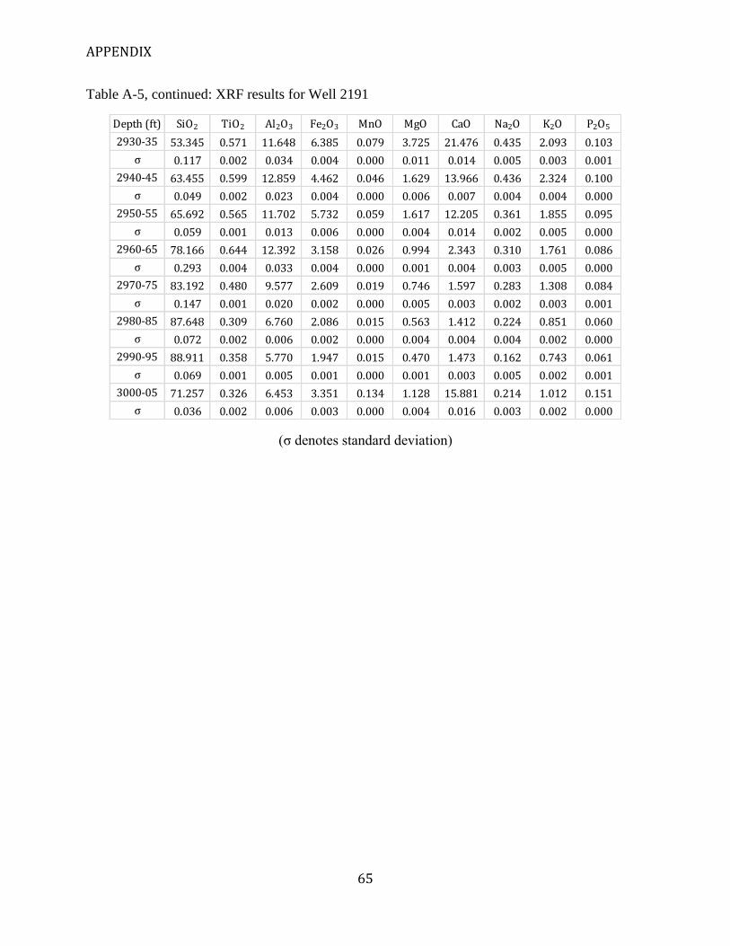
APPENDIX

65

Table A-5, continued: XRF results for Well 2191

(σ denotes standard deviation)

Depth (ft) SiO2 TiO2 Al2O3 Fe2O3 MnO MgO CaO Na2O K2O P2O5

2930-35 53.345 0.571 11.648 6.385 0.079 3.725 21.476 0.435 2.093 0.103

σ 0.117 0.002 0.034 0.004 0.000 0.011 0.014 0.005 0.003 0.001

2940-45 63.455 0.599 12.859 4.462 0.046 1.629 13.966 0.436 2.324 0.100

σ 0.049 0.002 0.023 0.004 0.000 0.006 0.007 0.004 0.004 0.000

2950-55 65.692 0.565 11.702 5.732 0.059 1.617 12.205 0.361 1.855 0.095

σ 0.059 0.001 0.013 0.006 0.000 0.004 0.014 0.002 0.005 0.000

2960-65 78.166 0.644 12.392 3.158 0.026 0.994 2.343 0.310 1.761 0.086

σ 0.293 0.004 0.033 0.004 0.000 0.001 0.004 0.003 0.005 0.000

2970-75 83.192 0.480 9.577 2.609 0.019 0.746 1.597 0.283 1.308 0.084

σ 0.147 0.001 0.020 0.002 0.000 0.005 0.003 0.002 0.003 0.001

2980-85 87.648 0.309 6.760 2.086 0.015 0.563 1.412 0.224 0.851 0.060

σ 0.072 0.002 0.006 0.002 0.000 0.004 0.004 0.004 0.002 0.000

2990-95 88.911 0.358 5.770 1.947 0.015 0.470 1.473 0.162 0.743 0.061

σ 0.069 0.001 0.005 0.001 0.000 0.001 0.003 0.005 0.002 0.001

3000-05 71.257 0.326 6.453 3.351 0.134 1.128 15.881 0.214 1.012 0.151

σ 0.036 0.002 0.006 0.003 0.000 0.004 0.016 0.003 0.002 0.000

APPENDIX

66

Table A-6: XRF results for Well 1780 samples

(σ denotes standard deviation)

Depth (ft) SiO2 TiO2 Al2O3 Fe2O3 MnO MgO CaO Na2O K2O P2O5

6270-80 54.452 0.924 16.470 6.180 0.039 2.124 16.049 0.920 2.533 0.148

σ 0.094 0.002 0.039 0.004 0.000 0.007 0.005 0.009 0.004 0.001

6280-90 46.115 0.799 13.898 5.624 0.048 1.992 28.274 0.798 2.093 0.189

σ 0.067 0.003 0.027 0.001 0.000 0.003 0.005 0.007 0.003 0.001

6290-00 58.951 0.990 20.360 6.818 0.053 2.105 6.107 0.821 3.468 0.159

σ 0.089 0.002 0.045 0.004 0.000 0.009 0.004 0.003 0.006 0.001

6300-10 58.946 0.920 18.880 8.284 0.146 2.067 6.625 0.860 2.798 0.305

σ 0.278 0.001 0.064 0.011 0.000 0.008 0.007 0.007 0.006 0.002

6310-20 53.668 0.856 16.314 6.950 0.068 2.092 16.261 0.866 2.391 0.374

σ 0.026 0.002 0.013 0.005 0.000 0.005 0.005 0.006 0.002 0.001

6320-30 56.263 0.870 17.113 7.428 0.099 2.217 11.869 0.912 2.441 0.625

σ 0.043 0.002 0.019 0.006 0.000 0.004 0.010 0.013 0.005 0.001

6330-40 57.627 0.877 17.272 6.764 0.084 2.108 10.811 0.995 2.574 0.699

σ 0.044 0.003 0.025 0.001 0.000 0.005 0.010 0.010 0.004 0.001

6340-50 59.117 0.876 17.796 6.317 0.054 2.059 9.601 0.829 2.558 0.596

σ 0.066 0.003 0.018 0.003 0.000 0.004 0.004 0.007 0.004 0.001

6350-60 59.560 0.931 18.126 6.075 0.047 1.994 9.174 0.830 2.618 0.456

σ 0.025 0.001 0.019 0.005 0.000 0.008 0.005 0.007 0.002 0.001

6360-70 62.721 1.012 19.853 7.607 0.039 1.883 2.932 0.858 2.738 0.198

σ 0.038 0.002 0.036 0.004 0.000 0.006 0.003 0.005 0.005 0.000

6370-80 61.830 1.001 19.810 7.894 0.048 1.939 3.540 0.842 2.737 0.191

σ 0.021 0.002 0.021 0.003 0.000 0.006 0.005 0.003 0.005 0.001

6380-90 61.488 1.001 19.833 7.543 0.043 1.960 4.160 0.823 2.776 0.206

σ 0.045 0.002 0.017 0.003 0.000 0.006 0.003 0.003 0.004 0.001

6390-00 61.423 0.980 22.035 8.144 0.073 1.800 1.441 0.808 2.991 0.131

σ 0.064 0.002 0.043 0.005 0.000 0.003 0.003 0.001 0.003 0.001

6400-10 61.137 0.979 21.530 7.965 0.098 1.823 2.370 0.834 2.967 0.128

σ 0.072 0.003 0.031 0.005 0.000 0.005 0.002 0.005 0.006 0.001

6410-20 60.317 0.953 19.710 8.644 0.081 1.957 4.116 0.899 2.907 0.233

σ 0.147 0.002 0.066 0.005 0.000 0.004 0.007 0.006 0.005 0.000

6420-30 64.380 0.836 17.100 6.707 0.059 2.085 4.272 0.894 3.008 0.440

σ 0.159 0.004 0.048 0.003 0.000 0.003 0.004 0.007 0.008 0.001

6430-40 61.780 0.871 18.772 7.020 0.070 2.368 4.428 0.893 3.259 0.330

σ 0.183 0.002 0.064 0.006 0.000 0.008 0.002 0.011 0.004 0.002

6440-50 62.142 0.884 18.691 7.870 0.084 2.087 3.599 0.876 3.222 0.335

σ 0.243 0.001 0.085 0.006 0.000 0.009 0.003 0.006 0.004 0.001

6450-60 64.803 0.857 18.215 5.796 0.044 2.023 3.668 0.883 3.219 0.275

σ 0.253 0.003 0.048 0.006 0.000 0.005 0.005 0.007 0.008 0.002

APPENDIX

67

Table A-6, continued: XRF results for Well 1780 samples

(σ denotes standard deviation)

Depth (ft) SiO2 TiO2 Al2O3 Fe2O3 MnO MgO CaO Na2O K2O P2O5

6460-70 63.617 0.857 18.041 6.618 0.053 2.170 3.713 0.944 3.259 0.498

σ 0.049 0.003 0.027 0.005 0.000 0.006 0.003 0.005 0.003 0.001

6470-80 62.534 0.928 19.455 7.000 0.066 2.005 3.314 0.915 3.160 0.416

σ 0.035 0.001 0.026 0.004 0.000 0.005 0.008 0.007 0.005 0.001

6480-90 62.511 0.974 19.910 6.744 0.051 2.051 2.787 0.950 3.515 0.265

σ 0.067 0.001 0.026 0.007 0.000 0.008 0.007 0.008 0.008 0.001

6490-00 61.279 0.892 17.731 5.915 0.053 2.168 7.142 0.879 3.285 0.389

σ 0.109 0.002 0.014 0.001 0.000 0.008 0.007 0.011 0.003 0.001

6500-10 61.444 0.865 18.158 8.051 0.095 2.042 5.172 0.770 2.845 0.341

σ 0.088 0.001 0.018 0.006 0.000 0.004 0.007 0.008 0.002 0.002

6510-20 54.704 0.893 17.084 6.689 0.112 1.857 14.799 0.813 2.670 0.190

σ 0.091 0.002 0.026 0.005 0.000 0.006 0.017 0.004 0.005 0.000

6520-30 51.653 0.441 7.332 3.617 0.105 1.365 33.618 0.327 1.314 0.104

σ 3.323 0.002 0.010 0.004 0.001 0.005 0.019 0.002 0.004 0.001

6530-40 56.800 0.490 8.098 4.449 0.115 1.406 26.731 0.372 1.251 0.160

σ 4.631 0.003 0.006 0.005 0.001 0.005 0.024 0.003 0.004 0.001

6540-50 56.072 0.778 16.499 8.607 0.191 2.024 12.559 0.563 2.332 0.217

σ 0.913 0.003 0.022 0.004 0.001 0.004 0.008 0.005 0.003 0.001

6550-60 61.401 0.809 15.786 6.865 0.135 1.813 9.651 0.610 2.520 0.242

σ 0.141 0.002 0.047 0.006 0.000 0.008 0.007 0.004 0.002 0.001

6560-70 59.054 0.789 15.668 8.203 0.140 1.824 10.937 0.608 2.470 0.151

σ 1.964 0.001 0.027 0.005 0.000 0.004 0.009 0.005 0.006 0.001

APPENDIX

68

Table A-7: XRF results for Well 15668 samples.

(σ denotes standard deviation)

Depth (ft) SiO2 TiO2 Al2O3 Fe2O3 MnO MgO CaO Na2O K2O P2O5

9013.0 63.229 0.870 19.978 5.889 0.025 2.304 2.723 0.944 3.704 0.106

σ 0.149 0.001 0.257 0.002 0.000 0.013 0.004 0.006 0.008 0.001

9022.8 66.876 0.900 15.584 5.195 0.030 1.651 4.830 0.933 3.276 0.428

σ 2.066 0.002 0.146 0.003 0.000 0.022 0.009 0.010 0.007 0.002

9033.0 15.444 0.382 4.345 2.645 0.049 4.314 71.100 0.504 0.969 0.085

σ 0.036 0.002 0.055 0.003 0.000 0.010 0.018 0.007 0.002 0.000

9044.0 3.237 0.052 0.511 0.627 0.042 0.884 94.094 0.081 0.130 0.174

σ 0.030 0.001 0.002 0.001 0.000 0.005 0.053 0.003 0.001 0.001

9053.0 63.565 0.859 19.606 4.596 0.019 2.020 4.503 0.672 3.871 0.152

σ 0.048 0.002 0.021 0.005 0.000 0.005 0.002 0.004 0.006 0.000

9062.7 12.685 0.084 1.142 0.575 0.056 0.704 84.170 0.123 0.174 0.179

σ 0.008 0.002 0.003 0.001 0.001 0.003 0.036 0.002 0.001 0.001

9073.0 86.754 0.027 0.157 0.612 0.015 0.355 11.848 0.132 0.020 0.039

σ 0.093 0.000 0.002 0.000 0.000 0.003 0.004 0.002 0.001 0.000

APPENDIX

69

Table A-8: XRF trace element data for samples from Well 2191.

(σ denotes standard deviation)

Depth (ft) Formation V Cr Ni Cu Zn Rb Sr Y Zr Nb Ba Mo U

2740-45 Neal 120.09 184.16 59.38 22.77 124.56 91.30 725.92 28.57 134.60 8.93 300.68 6.03 3.35

σ 3.38 2.61 0.40 1.02 0.80 0.40 0.80 0.49 0.49 0.63 10.98 0.49 0.00

2750-55 Neal 172.33 251.09 73.00 28.32 163.93 121.45 563.23 34.51 141.36 11.28 438.91 7.96 4.42

σ 1.47 1.79 0.63 0.49 0.75 0.40 1.33 0.75 0.40 0.40 11.34 0.40 0.00

2760-65 Neal 215.77 252.80 75.17 26.83 181.17 130.17 540.86 35.70 148.80 11.75 334.85 8.87 4.44

σ 3.26 3.03 1.17 0.98 1.50 0.49 0.98 0.40 0.40 0.49 16.02 0.00 0.00

2770-75 Neal 211.91 351.17 90.21 34.19 197.52 126.20 547.11 39.14 148.48 11.47 526.41 10.35 4.50

σ 2.42 1.72 0.75 0.80 1.02 0.40 1.36 0.40 0.00 0.40 22.51 0.40 0.00

2780-85 Neal 285.61 448.34 111.97 42.52 252.67 133.79 427.42 45.19 152.71 12.24 491.31 14.69 4.45

σ 2.15 2.04 1.50 0.40 1.10 0.40 0.63 0.49 0.40 0.00 11.25 0.40 0.00

2790-95 Neal 307.87 454.37 115.42 43.95 229.07 142.06 371.79 40.84 171.58 14.65 505.20 14.43 4.44

σ 1.62 3.32 0.63 0.49 1.50 0.63 0.89 0.40 0.80 0.40 19.81 0.00 0.00

2800-05 Neal 260.68 350.17 95.75 34.59 184.35 146.85 382.98 41.29 159.13 13.84 660.84 10.04 4.46

σ 2.42 1.17 0.40 0.63 0.75 0.49 0.75 0.63 0.49 0.49 9.28 0.00 0.00

2810-15 Neal 181.64 303.77 77.93 24.93 134.29 138.69 247.84 33.31 172.84 14.46 272.77 5.87 4.19

σ 2.58 2.76 0.49 0.40 0.40 0.49 0.49 0.40 0.00 0.40 12.74 0.49 0.00

2820-25 Neal 172.48 296.21 78.36 26.05 131.51 137.39 256.09 32.56 161.97 14.08 326.88 5.88 4.20

σ 3.60 1.26 1.36 0.98 0.75 0.40 0.75 0.00 0.75 0.49 6.94 0.49 0.00

2830-35 Neal 179.10 337.24 84.26 31.76 153.06 136.76 271.19 33.03 160.89 14.82 289.40 6.56 4.23

σ 1.33 1.74 0.80 0.63 1.36 0.40 0.40 0.98 0.00 0.00 8.48 0.40 0.00

2840-45 Neal 161.72 295.79 75.97 28.51 139.38 126.19 287.06 34.69 178.96 13.62 272.38 6.38 4.26

σ 3.16 2.45 0.80 0.40 1.10 0.49 0.98 0.49 0.40 0.40 9.88 0.00 0.00

2850-55 Neal 186.15 344.33 89.49 35.13 171.16 129.54 347.46 39.38 188.61 13.65 315.02 8.95 4.47

σ 1.02 3.31 0.63 0.49 0.00 0.75 1.02 0.40 0.49 0.40 4.96 0.00 0.00

2860-65 Neal 203.25 394.07 99.52 41.10 195.26 119.73 358.08 45.32 192.37 13.33 356.97 12.22 4.44

σ 2.76 2.14 1.02 0.63 1.17 0.40 0.49 0.75 0.40 0.00 20.77 0.00 0.00

2870-75 Neal 244.81 445.53 111.38 49.61 231.26 128.15 413.38 50.52 194.29 14.01 391.56 13.78 4.59

σ 1.47 1.26 0.63 0.98 0.49 1.02 0.89 0.63 0.75 0.40 14.87 0.00 0.00

2880-85 Neal 225.02 325.40 93.48 37.84 174.05 158.70 432.46 41.18 187.63 15.14 489.22 7.79 4.45

σ 1.83 0.80 1.10 0.63 0.49 0.80 0.49 0.63 1.02 0.49 9.07 0.00 0.00

2890-95 Neal 200.22 226.52 70.65 24.13 131.96 142.17 431.09 37.83 147.61 13.70 267.17 5.65 4.35

σ 2.14 3.61 0.63 0.75 1.02 0.40 1.02 0.40 0.40 0.49 11.72 0.40 0.00

2900-05 Neal 230.39 293.73 87.61 30.23 152.05 161.10 342.72 37.96 155.58 15.45 329.48 6.62 4.41

σ 2.04 2.64 0.49 1.02 1.17 0.00 0.49 0.49 0.00 0.00 11.57 0.00 0.00

2910-15 Neal 195.78 318.39 83.32 30.48 164.16 155.58 450.04 36.81 156.94 13.55 360.84 7.90 4.52

σ 2.33 2.97 0.40 1.10 0.49 0.40 1.20 0.80 0.63 0.00 9.89 0.00 0.00

2920-25 Neal 211.70 433.26 112.01 45.92 232.76 147.41 318.56 41.22 178.10 14.56 454.32 10.98 4.48

σ 2.10 2.14 0.63 0.89 1.60 0.49 0.80 0.75 0.63 0.00 12.94 0.40 0.00

2930-35 Neal 107.14 155.15 50.56 31.54 119.43 94.85 357.61 23.42 173.93 9.51 275.74 6.96 3.48

σ 1.74 2.40 0.80 0.40 0.63 0.75 1.02 0.40 0.00 0.40 9.50 0.00 0.00

2940-45 Neal 91.07 113.45 37.37 23.50 71.38 97.56 287.54 25.06 222.87 9.62 242.57 4.48 3.36

σ 0.80 2.06 0.49 0.63 0.75 0.40 0.63 0.49 0.75 0.49 8.93 0.00 0.00

APPENDIX

70

Table A-8, continued: XRF trace element data for samples from Well 2191.

(σ denotes standard deviation)

Depth (ft) Formation V Cr Ni Cu Zn Rb Sr Y Zr Nb Ba Mo U

2950-55 Floyd 90.07 109.21 44.36 29.95 72.73 83.99 263.91 24.99 209.64 9.68 205.59 5.63 3.38

σ 1.67 1.41 1.02 0.49 0.80 0.49 0.49 0.40 0.40 0.80 7.76 0.00 0.00

2960-65 Floyd 77.62 98.92 33.96 20.88 60.32 68.34 117.27 27.42 376.06 9.49 318.48 3.16 3.16

σ 2.87 2.40 0.40 0.75 0.40 0.40 0.40 0.00 0.49 0.00 7.13 0.00 0.00

2970-75 Floyd 64.62 107.22 28.75 18.04 52.03 50.36 98.40 21.61 323.75 7.34 274.02 4.20 3.15

σ 1.36 1.72 0.49 0.40 0.49 0.00 0.40 0.49 0.80 0.00 12.66 0.00 0.00

2980-85 Floyd 47.06 67.47 22.28 16.03 29.57 37.69 82.05 13.54 166.81 6.46 220.74 4.16 3.12

σ 0.75 1.60 0.49 1.02 0.49 0.40 0.40 0.00 0.40 0.40 11.56 0.00 0.00

2990-95 Floyd 43.25 82.34 20.79 17.05 27.03 29.73 74.85 17.67 331.01 5.20 249.92 4.16 3.12

σ 0.80 1.83 0.63 0.49 0.00 0.49 0.63 0.00 0.49 0.00 7.61 0.00 0.00

3000-05 Floyd 51.79 75.87 26.12 19.53 37.02 44.75 235.10 18.40 178.08 6.13 185.81 39.98 3.41

σ 1.85 1.94 0.63 1.17 0.49 0.49 0.63 0.40 0.40 0.49 7.47 0.40 0.00

APPENDIX

71

Table A-9: XRF trace element data for samples from Well 1780.

(σ denotes standard deviation)

Depth (ft) Formation V Cr Ni Cu Zn Rb Sr Y Zr Nb Ba Mo U

6270-80 Neal 142.60 125.72 53.09 29.99 126.39 149.71 434.03 40.20 195.69 15.77 282.99 4.22 4.44

σ 2.15 2.23 1.17 0.63 1.17 0.40 0.98 0.40 0.40 0.75 10.85 0.40 0.00

6280-90 Neal 124.76 129.30 50.45 28.63 115.21 125.67 643.78 39.77 175.20 13.18 234.29 5.68 4.54

σ 1.83 0.75 0.49 1.17 0.49 0.49 1.36 0.63 0.40 0.49 4.83 0.00 0.00

6290-00 Neal 151.50 147.02 65.51 49.72 123.12 183.08 295.75 40.76 176.68 17.07 420.36 4.27 4.27

σ 2.53 1.94 0.49 0.49 0.49 0.49 0.75 0.40 0.49 0.00 8.67 0.00 0.00

6300-10 Neal 139.31 158.82 63.53 32.18 139.10 154.88 346.51 48.37 183.74 15.57 385.33 5.19 4.15

σ 1.33 1.26 1.33 0.89 1.10 0.98 1.33 0.80 0.63 0.00 16.39 0.00 0.00

6310-20 Neal 135.62 182.43 62.26 30.91 140.85 137.80 445.40 45.93 182.64 14.15 213.77 5.44 4.35

σ 1.36 1.74 0.75 0.80 1.02 0.49 0.40 0.40 0.75 0.00 4.72 0.00 0.00

6320-30 Neal 135.58 181.78 62.66 31.65 139.65 137.29 412.31 50.47 188.40 14.33 258.12 5.77 4.28

σ 2.32 2.61 2.06 1.20 1.02 0.49 0.49 0.40 0.40 0.49 8.31 0.49 0.00

6330-40 Neal 178.51 246.65 78.81 37.88 189.62 140.63 456.52 56.82 188.31 14.15 289.11 8.49 4.35

σ 3.41 1.85 0.80 0.75 0.40 0.75 0.80 0.40 0.63 0.00 11.20 0.40 0.00

6340-50 Neal 203.80 261.38 81.04 35.20 199.67 132.75 464.31 51.06 190.11 14.34 315.70 8.69 4.35

σ 3.01 2.58 1.02 0.80 0.98 0.40 0.49 0.00 0.63 0.40 10.13 0.00 0.00

6350-60 Neal 197.46 235.57 75.35 32.36 179.95 141.61 441.89 50.08 200.34 15.73 305.60 7.76 4.43

σ 2.56 2.58 0.89 0.40 1.36 0.75 0.75 0.75 0.40 0.40 10.57 0.00 0.00

6360-70 Neal 159.38 159.59 65.20 30.90 137.86 164.28 287.86 49.43 196.88 17.90 314.28 4.69 4.26

σ 3.38 1.47 0.98 0.89 0.49 0.40 0.75 0.49 0.40 0.40 8.79 0.49 0.00

6370-80 Neal 164.73 167.08 66.53 33.37 139.91 163.23 315.55 45.78 196.18 17.11 344.65 4.92 4.28

σ 1.10 2.32 0.98 0.40 1.33 0.49 0.63 0.40 1.02 0.00 6.55 0.49 0.00

6380-90 Neal 170.84 169.11 66.78 34.47 142.23 163.26 330.63 47.48 197.51 17.56 320.88 4.99 4.34

σ 2.58 2.68 0.49 0.75 0.98 0.49 0.63 0.75 0.40 0.40 12.96 0.49 0.00

6390-00 Neal 212.74 222.23 75.87 33.63 155.62 171.14 257.58 43.76 171.58 17.89 361.04 5.39 4.31

σ 1.50 2.23 0.80 0.40 0.80 0.75 1.10 0.49 0.40 0.49 5.69 0.00 0.00

6400-10 Neal 211.05 207.37 72.95 33.55 149.57 168.62 265.16 45.46 175.55 17.10 344.17 5.19 4.33

σ 3.22 2.42 0.49 0.63 0.75 0.75 0.00 0.63 0.75 0.40 4.90 0.40 0.00

6410-20 Neal 193.88 241.97 78.03 37.60 170.05 162.40 314.53 48.31 182.73 17.05 362.18 5.46 4.37

σ 1.50 1.50 1.02 1.20 0.49 0.80 1.17 0.40 0.75 0.49 17.57 0.00 0.00

6420-30 Neal 199.43 420.58 104.93 46.49 243.10 139.90 359.97 48.88 167.06 14.34 411.46 9.12 4.34

σ 2.24 4.49 0.80 0.40 0.98 0.75 1.36 0.00 0.75 0.75 13.20 0.49 0.00

6430-40 Neal 196.68 366.37 97.03 43.29 212.56 156.86 348.10 46.78 166.87 15.01 422.29 8.05 4.35

σ 2.79 1.94 0.75 0.98 1.02 0.40 0.63 0.63 0.49 0.40 8.38 0.49 0.00

6440-50 Neal 201.41 368.16 99.62 45.12 221.25 159.99 333.72 54.06 174.82 15.26 411.98 8.72 4.36

σ 2.79 3.87 1.50 1.02 0.00 0.40 0.98 0.49 0.49 0.63 7.13 0.00 0.00

6450-60 Neal 200.92 408.24 107.29 47.78 250.83 149.94 348.52 44.36 171.27 14.72 413.36 10.02 4.27

σ 1.85 3.49 0.49 0.40 0.98 0.49 0.98 0.49 0.49 0.75 14.15 0.49 0.00

6460-70 Neal 201.58 432.90 109.30 52.39 253.53 151.99 392.80 55.62 175.49 14.66 426.01 10.78 4.31

σ 1.26 1.85 0.80 1.02 1.17 0.00 1.02 0.49 0.40 0.49 21.61 0.00 0.00

6470-80 Neal 196.06 342.84 93.64 45.64 220.49 158.99 349.26 51.85 185.13 16.07 397.47 8.57 4.29

σ 2.10 2.10 1.36 0.49 0.75 0.49 0.63 0.49 0.75 0.00 16.37 0.00 0.00

6480-90 Neal 241.90 451.04 118.09 57.62 285.67 171.09 361.98 52.34 197.26 16.71 459.84 12.32 4.40

σ 2.61 2.93 1.50 0.80 0.98 0.49 0.75 0.49 0.49 0.40 19.29 0.40 0.00

6490-00 Neal 235.71 607.93 148.13 69.71 344.07 151.26 405.95 52.28 188.12 14.52 434.33 15.42 4.47

σ 1.67 3.43 0.80 0.49 0.63 0.49 0.49 0.40 1.02 0.00 13.73 0.40 0.00

APPENDIX

72

Table A-9, continued: XRF trace element data for samples from Well 1780.

(σ denotes standard deviation)

Table A-10: XRF trace element data for samples from Well 15668.

(σ denotes standard deviation)

Depth (ft) Formation V Cr Ni Cu Zn Rb Sr Y Zr Nb Ba Mo U

6500-10 Neal 200.24 402.01 119.54 55.84 244.31 141.35 354.68 49.73 173.63 14.83 407.03 10.91 4.36

σ 2.06 3.44 1.36 0.75 1.10 0.80 0.40 0.49 0.75 0.49 4.62 0.00 0.00

6510-20 Neal 189.94 285.60 83.24 38.86 180.97 144.18 380.80 43.92 180.05 15.18 317.79 7.59 4.60

σ 2.99 3.07 1.02 0.40 1.02 0.80 1.17 0.40 0.49 0.40 14.84 0.49 0.00

6520-30 Neal 69.73 113.36 36.90 24.67 81.56 61.98 434.69 22.84 200.02 6.52 171.27 5.10 3.06

σ 3.44 1.72 0.75 0.40 1.41 0.75 0.80 0.49 0.40 0.49 21.23 0.00 0.00

6530-40 Neal 68.11 94.54 33.60 26.88 70.57 57.58 384.22 25.99 282.28 6.72 224.48 5.15 3.36

σ 1.17 1.85 1.26 0.63 0.63 0.49 0.89 0.40 1.10 0.63 9.97 0.49 0.00

6540-50 Neal 139.47 185.45 61.82 33.22 134.41 120.11 360.56 45.32 200.85 12.54 269.05 5.50 4.40

σ 3.25 1.36 1.94 0.98 0.40 0.40 0.75 0.40 0.49 0.49 5.68 0.00 0.00

6550-60 Neal 145.54 195.98 104.66 37.11 143.54 130.21 350.86 42.00 220.43 13.55 291.31 8.67 4.44

σ 1.90 3.50 0.75 0.49 0.75 0.75 0.40 0.40 0.49 0.40 9.26 0.40 0.00

6560-70 Neal 119.24 143.23 59.62 38.66 141.60 132.98 339.09 45.41 210.53 16.07 325.12 5.82 4.66

σ 2.42 2.76 1.17 0.75 1.02 0.40 0.40 0.63 0.40 0.40 20.44 0.00 0.00

Depth (ft) Formation V Cr Ni Cu Zn Rb Sr Y Zr Nb Ba Mo U

9013.0 Neal 209.96 589.39 106.84 45.39 187.39 180.17 415.51 34.92 175.51 14.90 317.27 10.47 4.66

σ 1.36 3.72 0.75 0.63 0.63 0.40 1.10 0.00 0.40 0.40 10.74 0.00 0.00

9022.8 Neal 215.05 778.13 163.86 92.84 460.46 152.31 377.40 56.21 210.53 16.06 432.10 21.33 5.02

σ 3.14 1.72 0.49 0.63 0.63 0.49 0.75 0.75 0.40 0.40 3.61 0.00 0.00

9033.0 Lewis 63.70 48.03 47.02 18.45 160.01 41.71 1019.21 15.67 154.70 5.31 60.67 11.38 3.79

σ 1.50 1.26 1.33 0.80 0.49 0.00 0.80 0.49 0.49 0.75 13.96 0.00 0.00

9044.0 Lewis 14.30 0.00 11.30 12.69 42.44 8.53 1370.72 9.23 90.18 -1.15 93.41 4.61 3.46

σ 2.24 2.40 1.60 1.55 1.47 0.49 1.36 0.63 0.75 0.63 21.15 0.63 0.00

9053.0 Neal 121.26 134.25 60.11 23.46 141.79 189.33 288.81 28.48 145.35 16.55 231.43 5.24 4.19

σ 1.94 1.33 0.80 0.80 1.20 0.75 0.75 0.40 0.40 0.40 15.72 0.00 0.00

9062.7 Lewis 22.04 25.36 13.75 19.44 34.84 8.06 745.41 20.86 64.70 0.71 130.36 5.69 3.56

σ 3.44 1.02 1.02 0.49 1.20 0.40 1.10 0.80 0.80 0.49 13.61 0.75 0.00

9073.0 Neal 6.61 0.00 7.30 10.95 7.98 2.05 317.29 3.19 22.81 3.19 36.50 4.56 3.42

σ 0.98 1.47 0.49 0.49 0.63 0.40 0.75 0.40 0.00 0.75 2.10 0.00 0.00

APPENDIX

73

Table A-11: Uniaxial stength test results for Well 15668 core samples.

d: diametral test; a: axial test; i: irregular lump; D: distance between platen contact points; L: length of the sample measured from the platen contact point to the edge of the sample; W: width; psi: pounds per square inch; N: load measured in Newton; Is: index strength; MPa: Mega-Pascal; F: correction factor; Is(50): index strength normalized to D=50mm

Top Depth Formation Test D (mm) L (mm) W (mm) psi Load (N) Is, MPa F Is(50), MPa

9016.9 Neal d 24.5 8.3 - 40 478.28 0.80 0.73 0.58

9016.9 Neal d 24.5 11.5 - 60 717.42 1.20 0.73 0.87

9016.9 Neal d 24.5 8.0 - 20 239.14 0.40 0.73 0.29

9021.0 Neal d 24.5 10.5 - 80 956.55 1.59 0.73 1.16

9021.0 Neal d 24.5 16.0 - 80 956.55 1.59 0.73 1.16

9022.8 Neal d 24.5 16.8 - 20 239.14 0.40 0.73 0.29

9022.8 Neal d 24.5 5.3 - 40 478.28 0.80 0.73 0.58

9024.2 Neal d 24.5 9.5 - 80 956.55 1.59 0.73 1.16

9024.2 Neal d 24.5 17.3 - 75 896.77 1.49 0.73 1.08

9033.5 Lewis d 24.5 22.0 - 975 11658.01 19.42 0.73 14.09

9044.6 Lewis d 24.5 23.3 - 675 8070.93 13.45 0.73 9.75

9062.9 Lewis d 24.5 17.3 - 2025 24212.79 40.34 0.73 29.26

9073.0 Lewis d 24.5 19.0 - 2475 29593.41 49.30 0.73 35.76

9013.0 Neal a 9.5 - 24.5 100 1195.69 4.03 0.47 1.91

9013.0 Neal a 11.5 - 24.5 120 1434.83 4.00 0.52 2.06

9013.0 Neal a 5 - 24.5 100 1195.69 7.67 0.35 2.72

9013.0 Neal a 8 - 24.5 120 1434.83 5.75 0.44 2.52

9014.0 Neal a 10 - 24.5 140 1673.97 5.37 0.48 2.60

9014.0 Neal a 8.5 - 24.5 160 1913.11 7.22 0.45 3.25

9016.9 Neal a 16.5 - 24.5 220 2630.53 5.11 0.61 3.10

9016.9 Neal a 6 - 24.5 80 956.55 5.11 0.39 1.97

9016.9 Neal a 12 - 24.5 220 2630.53 7.03 0.53 3.70

9016.9 Neal a 9 - 24.5 220 2630.53 9.37 0.46 4.33

9016.9 Neal a 12 - 24.5 260 3108.80 8.30 0.53 4.37

9016.9 Neal a 6 - 24.5 120 1434.83 7.67 0.39 2.95

9021.06 Neal a 9.5 - 24.5 220 2630.53 8.88 0.47 4.20

9021.0 Neal a 7 - 24.5 80 956.55 4.38 0.41 1.81

9021.0 Neal a 11 - 24.5 180 2152.25 6.27 0.51 3.17

9021.1 Neal a 14 - 24.5 280 3347.94 7.67 0.56 4.32

9021.0 Neal a 13 - 24.5 160 1913.11 4.72 0.55 2.57

9021.0 Neal a 20 - 24.5 440 5261.05 8.43 0.66 5.58

APPENDIX

74

Table A-11, continued: Uniaxial stength test results for Well 15668 core samples.

d: diametral test; a: axial test; i: irregular lump; D: distance between platen contact points; L: length of the sample measured from the platen contact point to the edge of the sample; W: width; psi: pounds per square inch; N: load measured in Newton; Is: index strength; MPa: Mega-Pascal; F: correction factor; Is(50): index strength normalized to D=50mm

Top Depth Formation Test D (mm) L (mm) W (mm) psi Load (N) Is, MPa F Is(50), MPa

9022.8 Neal a 12 - 24.5 280 3347.94 8.94 0.53 4.71

9022.8 Neal a 12 - 24.5 200 2391.39 6.39 0.53 3.36

9022.8 Neal a 7 - 24.5 160 1913.11 8.76 0.41 3.62

9022.8 Neal a 14 - 24.5 140 1673.97 3.83 0.56 2.16

9022.8 Neal a 16 - 24.5 180 2152.25 4.31 0.60 2.58

9022.8 Neal a 4 - 24.5 80 956.55 7.67 0.32 2.46

9024.2 Neal a 8 - 24.5 180 2152.25 8.62 0.44 3.78

9024.2 Neal a 7 - 24.5 180 2152.25 9.86 0.41 4.07

9024.2 Neal a 6 - 24.5 130 1554.40 8.30 0.39 3.20

9024.2 Neal a 8 - 24.5 160 1913.11 7.67 0.44 3.36

9024.2 Neal a 11 - 24.5 300 3587.08 10.45 0.51 5.29

9024.2 Neal a 10 - 24.5 200 2391.39 7.67 0.48 3.72

9024.2 Neal a 6 - 24.5 120 1434.83 7.67 0.39 2.95

9044.6 Lewis a 20 - 24.5 40 478.28 0.77 0.66 0.51

9044.6 Lewis a 23 - 24.5 80 956.55 1.33 0.71 0.94

9062.9 Lewis a 15 - 24.5 840 10043.82 21.47 0.58 12.49

9073.0 Lewis a 8 - 24.5 200 2391.39 9.58 0.44 4.20

9062.9 Lewis i 14 17.0 24.5 700 8369.85 13.81 0.56 7.79

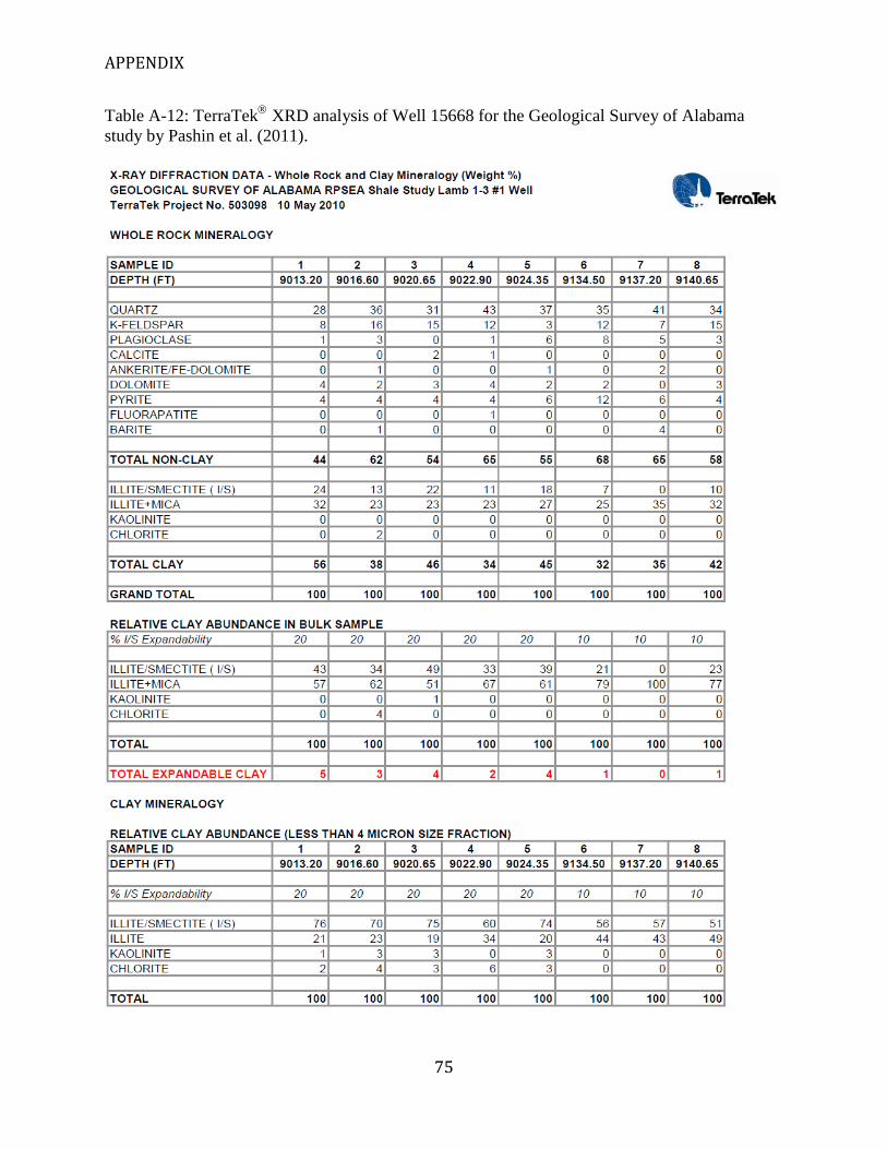
APPENDIX

75

Table A-12: TerraTek

XRD analysis of Well 15668 for the Geological Survey of Alabama

study by Pashin et al. (2011).

APPENDIX

76

Figure A-1: Correlation coefficient matrix for the Neal shale.

APPENDIX

77

Figure A-2: Correlation coefficient matrix for the Lewis Limestone.