Assessment of Macroeconomic Modeling in NEMS Sensitivity Studies with the NEMS Macroeconomic Model October 29, 2010 DOE/NETL-2010/1426

ii

Disclaimer

This report was prepared as an account of work sponsored by an agency of the United States Government. Neither the United States Government nor any agency thereof, nor any of their employees, makes any warranty, express or implied, or assumes any legal liability or responsibility for the accuracy, completeness, or usefulness of any information, apparatus, product, or process disclosed, or represents that its use would not infringe privately owned rights. Reference therein to any specific commercial product, process, or service by trade name, trademark, manufacturer, or otherwise does not necessarily constitute or imply its endorsement, recommendation, or favoring by the United States Government or any agency thereof. The views and opinions of authors expressed therein do not necessarily state or reflect those of the United States Government or any agency thereof.

iii

Assessment of Macroeconomic

Modeling in NEMS

DOE/NETL-2010/1426

Sensitivity Studies with the NEMS Macroeconomic Model

October 29, 2010

NETL Contact:

Rodney A. Geisbrecht Senior Analyst

Office of Systems Analyses and Planning

National Energy Technology Laboratory www.netl.doe.gov

iv

This page intentionally left blank

v

Table of Contents

Summary ....................................................................................................................................... 1 Background .................................................................................................................................. 2 Methodology................................................................................................................................. 3

Global Insight Macroeconomic Model and EVIEWS ......................................................... 3

NEMS Energy Prices and Consumptions File ..................................................................... 4

EVIEWS Sensitivity Calculations .......................................................................................... 4

Results and Discussion............................................................................................................... 4 GDP Sensitivity to Selected Drivers ..................................................................................... 5

Relationship of GDP to Energy Prices - Short versus Long Term Concepts ............. 5

Elasticity of Real GDP to Energy Prices - Direct and Indirect Factors ...................... 6

Model Feasibility Domains ................................................................................................ 8

Exogenous Drivers in the Low and High Macro Side Cases......................................... 9

Total Factor Productivity - Exogenous Driver of Special Interest ........................... 11

Sensitivity of Other Metrics to Selected Drivers ............................................................. 12

Conclusions and Recommendations ..................................................................................... 14 Appendix ..................................................................................................................................... 18

Excerpts of EVIEWS Drivers.PRG for Sensitivity Studies .............................................. 18

vi

Prepared by:

Rodney A. Geisbrecht Office of Systems Analyses and Planning National Energy Technology Laboratory

vii

Acknowledgements Phil DiPietro, Director of Situational Analysis and Benefits Division, Office of Systems Analyses and Planning, and Charles Zelek, Team Leader, Benefits Team, provided valuable guidance and encouragement in this task.

1

Summary This paper summarizes results of an exploratory study of how the macroeconomic impacts of energy prices and consumptions are modeled in the National Energy Modeling System (NEMS), the key modeling system used by the Energy Information Administration (EIA) to prepare the Annual Energy Outlook and Service Report Side Cases covering such issues as proposed climate change legislation and differing outlooks for world crude oil supplies. Sensitivity studies were used to quantify the impacts of energy prices and consumptions on metrics of national prosperity, such as real GDP. A secondary purpose of this report is to document methodology, so that additional studies can be undertaken by others in a practical and efficient fashion.

A primary motivation for this study is a perceived insensitivity of the macroeconomic model in NEMS to energy prices when high-world-oil-price or climate-change-policy scenarios are compared to business- as-usual scenarios such as the Annual Energy Outlooks. A key finding was that observed sensitivities are partly a reflection of demand elasticities in the demand models of NEMS, since these demands are used to overwrite endogenous consumptions in the macroeconomic model. The macroeconomic model in NEMS is the IHS/Global Insight mid-term forecast model of the U.S. economy (hereafter called the GI macro model), generally regarded as a best-in-class model. Another key finding was that the GI macro model, as implemented in NEMS, “fails-to-solve” when prices increase beyond a certain point without sufficient reductions in consumption. The GI macro model’s internal reaction functions, or elasticities of consumptions with respect to prices, are effectively replaced by those from the NEMS demand models through the use of NEMS derived consumption overwrites. Although NEMS based reaction functions are generally believed to be consistent with the GI model’s reactions functions, and both are believed to be more or less valid in business as usual scenarios, the existence of a “failure-to-solve” limit, as with any algorithm, implies a potential bias to only model scenarios within the model’s feasibility domain. In the case at hand, the potential bias would be for efficiency and conservation in climate change and energy security scenarios with high energy prices. A final key finding was that certain exogenous drivers in the GI macro model, which exert a profound impact on macroeconomic growth and are typically varied between macroeconomic growth scenarios, are assumed to be independent of energy prices. One such driver examined in this study is total factor productivity (TFP). Based upon available data and the literature, TFP may not be entirely independent of energy prices.

With respect to the sensitivity of real GDP to energy prices, three types of elasticities were estimated to reflect the integration of the GI macro model in NEMS: (1) a direct elasticity with respect to prices in the GI macro model at constant consumptions; (2) an indirect elasticity reflecting the combined effect of an elasticity with respect to consumptions in the GI macro model and an elasticity of demands with respect to prices in the NEMS demand models; (3) a hypothetical indirect elasticity not currently modeled in NEMS, reflecting the combined effect of an elasticity with respect to total factor productivity in the GI macro model and an assumed elasticity of total factor productivity with respect to prices. Some scenarios examined resulted in annual real GDP losses in 2030 as great as 15 %, or more than 3 trillion dollars (constant 2000 dollars) when hypothetical impacts to total factor productivity were combined with the impacts of energy prices and consumptions.

2

The methodology developed in this study greatly facilitated experimentation with the macro model and its implementation in NEMS, enabling sensitivity studies to be completed in minutes on a laptop rather than the tens of hours that would be needed on a workstation for a single, fully integrated NEMS run.

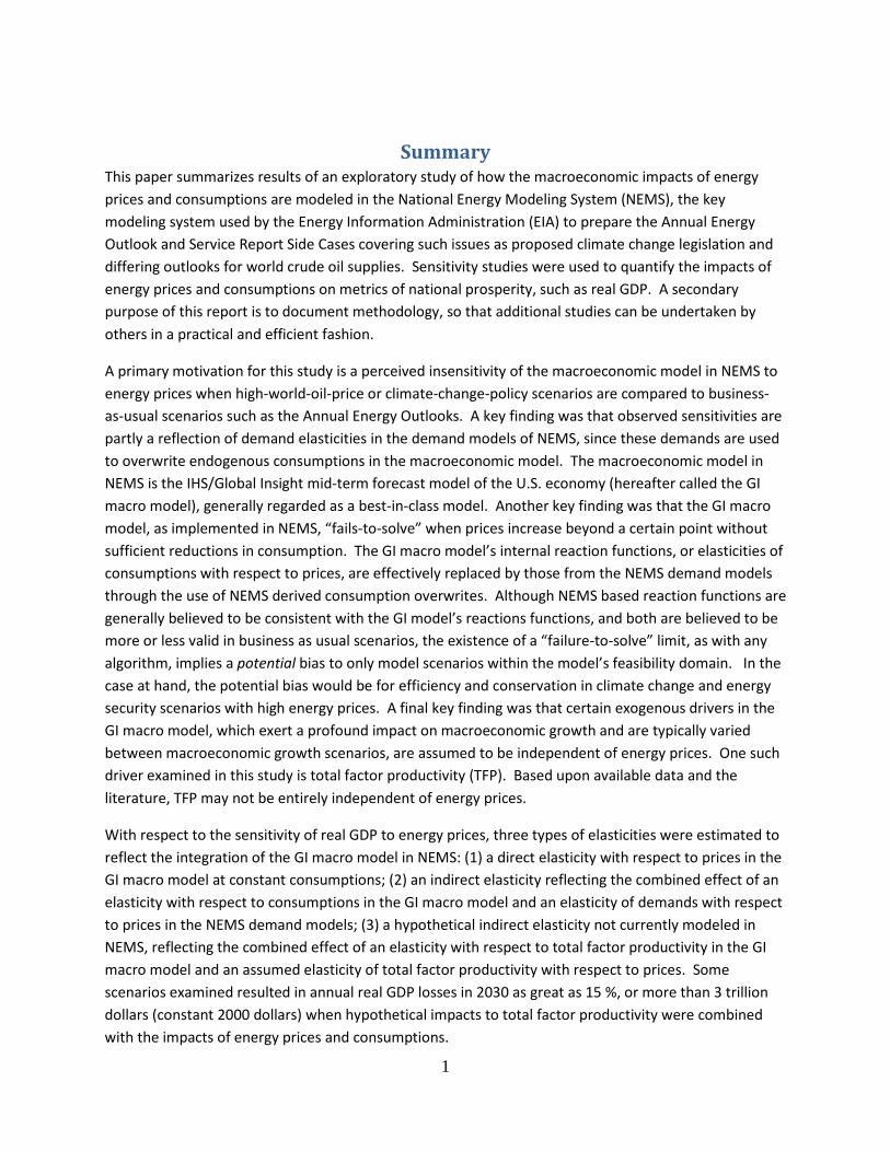
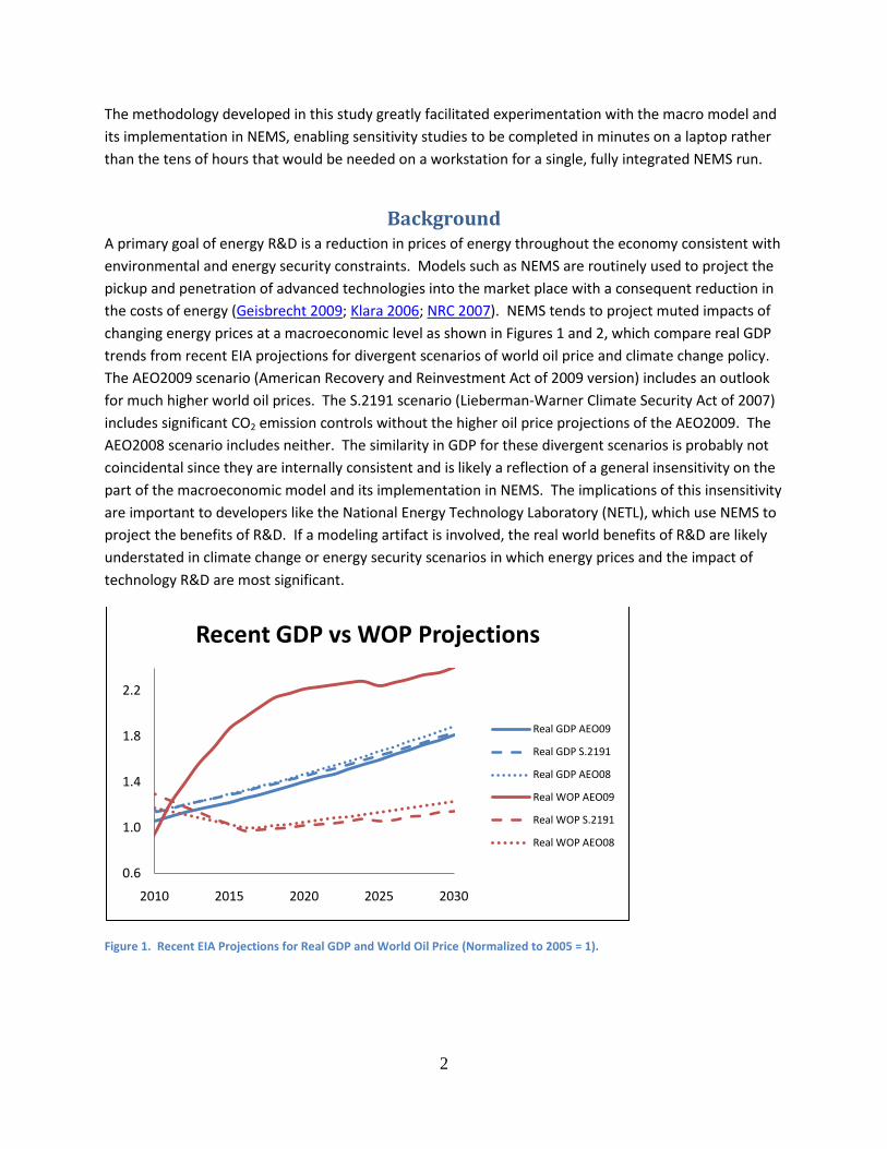
Background A primary goal of energy R&D is a reduction in prices of energy throughout the economy consistent with environmental and energy security constraints. Models such as NEMS are routinely used to project the pickup and penetration of advanced technologies into the market place with a consequent reduction in the costs of energy (Geisbrecht 2009; Klara 2006; NRC 2007). NEMS tends to project muted impacts of changing energy prices at a macroeconomic level as shown in Figures 1 and 2, which compare real GDP trends from recent EIA projections for divergent scenarios of world oil price and climate change policy. The AEO2009 scenario (American Recovery and Reinvestment Act of 2009 version) includes an outlook for much higher world oil prices. The S.2191 scenario (Lieberman-Warner Climate Security Act of 2007) includes significant CO2 emission controls without the higher oil price projections of the AEO2009. The AEO2008 scenario includes neither. The similarity in GDP for these divergent scenarios is probably not coincidental since they are internally consistent and is likely a reflection of a general insensitivity on the part of the macroeconomic model and its implementation in NEMS. The implications of this insensitivity are important to developers like the National Energy Technology Laboratory (NETL), which use NEMS to project the benefits of R&D. If a modeling artifact is involved, the real world benefits of R&D are likely understated in climate change or energy security scenarios in which energy prices and the impact of technology R&D are most significant.

Figure 1. Recent EIA Projections for Real GDP and World Oil Price (Normalized to 2005 = 1).

0.6

1.0

1.4

1.8

2.2

2010 2015 2020 2025 2030

Recent GDP vs WOP Projections

Real GDP AEO09

Real GDP S.2191

Real GDP AEO08

Real WOP AEO09

Real WOP S.2191

Real WOP AEO08

3

Figure 2. Recent EIA Projections for Real GDP and CO2 Emissions (Normalized to 2005 = 1). CO2 emissions are a proxy for alternative climate change policies and the resulting impacts on energy costs.

Methodology

Global Insight Macroeconomic Model and EVIEWS The framework for integrating macroeconomic effects with the energy supply and demand models in NEMS is described in EIA’s model documentation (EIA 2010), of which the following is a brief synopsis. The macro model in NEMS is the IHS/Global Insight mid-term forecast model of the U.S. economy (hereafter called the GI macro model). The GI macro model is contained in an EVIEWS work file which contains the model object and associated data objects. The GI macro model used in the AEO2009 (M_US2008A) consists of 1,727 equations and 2,022 variables (295 exogenous and 1,727 endogenous) where each variable is a serial object holding quarterly values from 1959Q1 to 2039Q4. The complex econometric nature of the model’s equations ultimately dictated a methodology based on empirical sensitivity studies.

EVIEWS is a Windows based forecasting and analysis package that integrates estimation, forecasting, statistical analysis, graphics, data management, and simulation, licensed by QMS, Inc. Procedures are implemented by issuing commands interactively or batch-wise in a “drivers” file (DRIVERS.PRG). In the NEMS framework, this file is scripted by NEMS immediately prior to executing the GI macro model as an external process. Understanding the command language is required to edit the drivers file and thereby define a sensitivity case, known as scenarios in EVIEWS. A powerful functionality is provided in EVIEWS to define, execute, and archive scenarios, consisting of alternate values for select variables. Depending on the nature of the variable, the alternate values are imposed as an override of an exogenous driver variable or an exclusion of an endogenous solution variable and its corresponding equation. Exclusions essentially convert an endogenous solution variable to an exogenous driver variable using the imposed values for the variable.

0.6

1.0

1.4

1.8

2.2

2010 2015 2020 2025 2030

Recent GDP vs CO2 Projections

Real GDP AEO09

Real GDP S.2191

Real GDP AEO08

Total CO2 AEO09

Total CO2 S.2191

Total CO2 AEO08

4

NEMS Energy Prices and Consumptions File Another file scripted by NEMS just prior to execution of the GI macro model is a “NEMS solutions” file (ALTDATA.WK1), which forms part of the interface between the GI macro model and the rest of NEMS. This file contains energy prices and consumptions as determined in the supply and demand models of NEMS that are then imposed on the GI macro model as exclusions of endogenous solution variables. EVIEWS reads this file, translates annual changes in NEMS variables into scaled changes in corresponding macro model variables, and finally executes the GI macro model. Projected time trends from NEMS are spliced onto historical trends from GI for the auto-regressed, or lagged, variables of the GI macro model.

EVIEWS Sensitivity Calculations For sensitivity studies, it is neither necessary nor productive to use fully integrated NEMS simulations. Because of how it is implemented (external, standalone process) the GI macro model can be used in a standalone fashion for sensitivity studies, condensing run times from tens of hours on a workstation to minutes on a laptop with EVIEWS installed. The run folder only needs to include MCEVWORK.WF1 (GI macro model), and three files from a baseline run of NEMS: DRIVERS.PRG (NEMS output requiring edits with a text editor); ALTDATA.WK1 (NEMS output requiring no edits); and MCHIGHLO.XLS (NEMS input requiring no edits)1

Results and Discussion

. Sensitivity studies are defined by editing DRIVERS.PRG. EVIEWS program language commands are inserted that declare sensitivity scenarios and overrides and exclusions of variables (see the EVIEWS program documentation and user help manuals). Sensitivity studies vary the time trends for how a driver variable is projected to change, splicing these trends onto the historical trends. Excerpts of a typical DRIVERS.PRG edited for sensitivity studies are shown in the Appendix, where five scenarios are defined, starting with the Baseline Scenario (S-1) that applies NEMS derived overwrites for energy prices and consumptions from AEO2009. Each subsequent scenario incorporates the previous scenarios, such that S-2 consumption reductions are added to the S-1 specifications, and S-3 price increases are added to the S-2 specifications. S-4 is a null (placeholder) scenario related to proprietary exogenous variables used in the GI and EIA macro side cases; in the studies reported herein, no variables were changed. S-5 is a scenario that includes variations in exogeneous drivers of special interest because of their possible dependency on energy prices.

Simulations were undertaken to examine the sensitivity of the GI macro model and its implementation in the NEMS framework to energy prices and consumptions, parsed as inputs to the macro model from the NEMS supply and demand models. Trends were determined for those metrics generally believed to be indicative of prosperity, such as real GDP growth. Changes in energy prices and consumptions were specified via exclusions of endogenous solution variables in the GI macro model. The baseline for these simulations is the AEO2009 including the American Recovery and Reinvestment Act of 2009, hereafter referred to as Scenario 1 (S-1).

1 MCHIGHLO.XLS, a “macro side cases” file read by EVIEWS, contains ratios of key GI macro model outputs from GI’s proprietary low or high macro forecast to the baseline forecast. These factors are used only if a macro side case is indicated in DRIVERS.PRG, as discussed later.

5

The impacts of additional variables were determined in subsequent sensitivity studies to gain insight into those observed for the primary NEMS energy price and consumption drivers. These variables included those likely used for the IHS/GI macro side cases. Changes in these variables were specified as overrides of exogenous driver variables. As discussed later, a major assumption in the NEMS implementation of the GI macro model is that these variables are independent of energy prices and consumptions, but some may not be entirely independent.

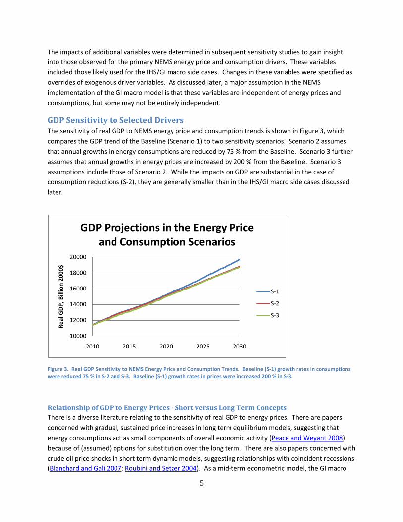
GDP Sensitivity to Selected Drivers The sensitivity of real GDP to NEMS energy price and consumption trends is shown in Figure 3, which compares the GDP trend of the Baseline (Scenario 1) to two sensitivity scenarios. Scenario 2 assumes that annual growths in energy consumptions are reduced by 75 % from the Baseline. Scenario 3 further assumes that annual growths in energy prices are increased by 200 % from the Baseline. Scenario 3 assumptions include those of Scenario 2. While the impacts on GDP are substantial in the case of consumption reductions (S-2), they are generally smaller than in the IHS/GI macro side cases discussed later.

Figure 3. Real GDP Sensitivity to NEMS Energy Price and Consumption Trends. Baseline (S-1) growth rates in consumptions were reduced 75 % in S-2 and S-3. Baseline (S-1) growth rates in prices were increased 200 % in S-3.

Relationship of GDP to Energy Prices - Short versus Long Term Concepts There is a diverse literature relating to the sensitivity of real GDP to energy prices. There are papers concerned with gradual, sustained price increases in long term equilibrium models, suggesting that energy consumptions act as small components of overall economic activity (Peace and Weyant 2008) because of (assumed) options for substitution over the long term. There are also papers concerned with crude oil price shocks in short term dynamic models, suggesting relationships with coincident recessions (Blanchard and Gali 2007; Roubini and Setzer 2004). As a mid-term econometric model, the GI macro

10000

12000

14000

16000

18000

20000

2010 2015 2020 2025 2030

Real

GD

P, B

illio

n 20

00$

GDP Projections in the Energy Price and Consumption Scenarios

S-1

S-2

S-3

6

model doesn’t necessarily conform to either viewpoint (software brochures mention the modeling of business cycles and recessions, but only as scenarios with crafted exogenous drivers featuring shocks and other volatilities).

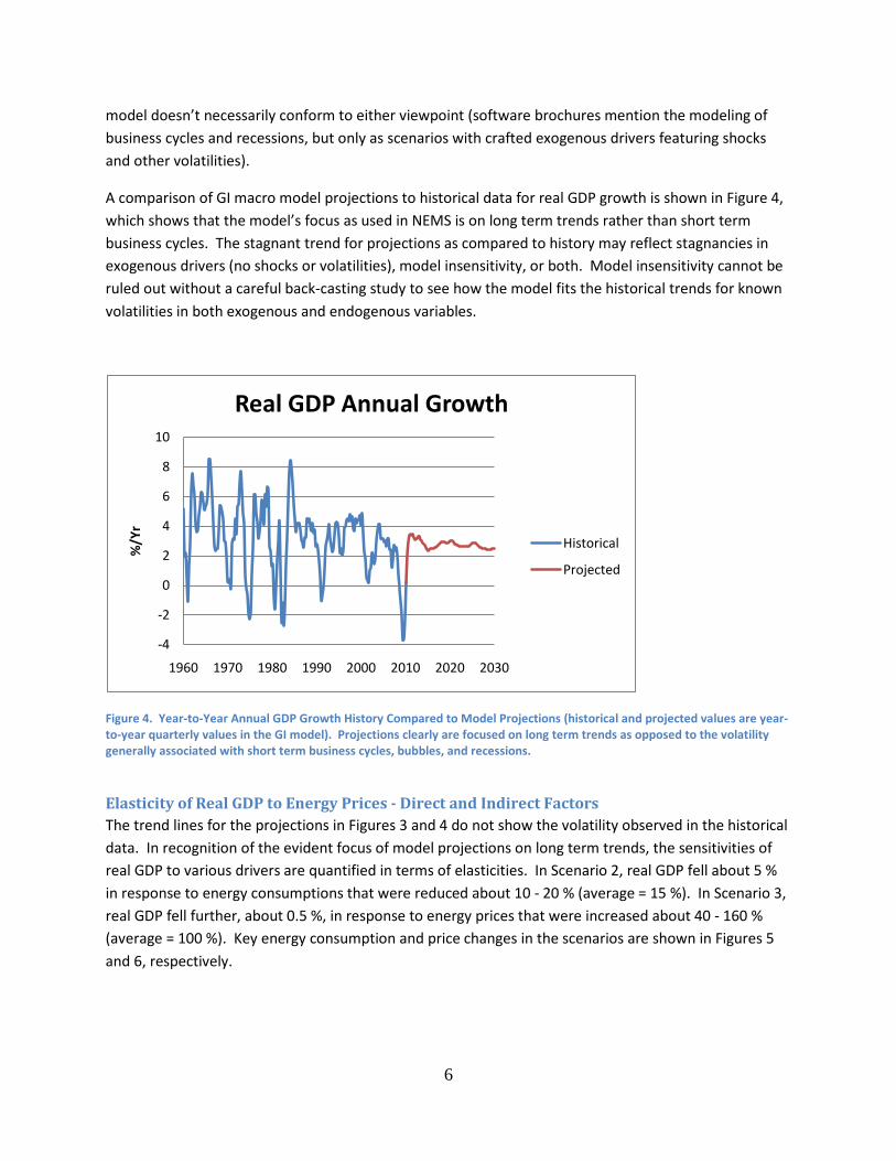
A comparison of GI macro model projections to historical data for real GDP growth is shown in Figure 4, which shows that the model’s focus as used in NEMS is on long term trends rather than short term business cycles. The stagnant trend for projections as compared to history may reflect stagnancies in exogenous drivers (no shocks or volatilities), model insensitivity, or both. Model insensitivity cannot be ruled out without a careful back-casting study to see how the model fits the historical trends for known volatilities in both exogenous and endogenous variables.

Figure 4. Year-to-Year Annual GDP Growth History Compared to Model Projections (historical and projected values are year-to-year quarterly values in the GI model). Projections clearly are focused on long term trends as opposed to the volatility generally associated with short term business cycles, bubbles, and recessions.

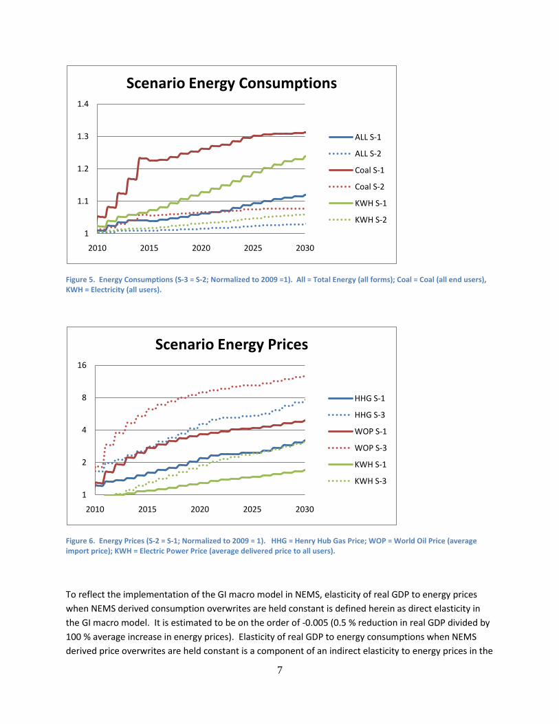
Elasticity of Real GDP to Energy Prices - Direct and Indirect Factors The trend lines for the projections in Figures 3 and 4 do not show the volatility observed in the historical data. In recognition of the evident focus of model projections on long term trends, the sensitivities of real GDP to various drivers are quantified in terms of elasticities. In Scenario 2, real GDP fell about 5 % in response to energy consumptions that were reduced about 10 - 20 % (average = 15 %). In Scenario 3, real GDP fell further, about 0.5 %, in response to energy prices that were increased about 40 - 160 % (average = 100 %). Key energy consumption and price changes in the scenarios are shown in Figures 5 and 6, respectively.

-4

-2

0

2

4

6

8

10

1960 1970 1980 1990 2000 2010 2020 2030

%/Y

r

Real GDP Annual Growth

Historical

Projected

7

Figure 5. Energy Consumptions (S-3 = S-2; Normalized to 2009 =1). All = Total Energy (all forms); Coal = Coal (all end users), KWH = Electricity (all users).

Figure 6. Energy Prices (S-2 = S-1; Normalized to 2009 = 1). HHG = Henry Hub Gas Price; WOP = World Oil Price (average import price); KWH = Electric Power Price (average delivered price to all users).

To reflect the implementation of the GI macro model in NEMS, elasticity of real GDP to energy prices when NEMS derived consumption overwrites are held constant is defined herein as direct elasticity in the GI macro model. It is estimated to be on the order of -0.005 (0.5 % reduction in real GDP divided by 100 % average increase in energy prices). Elasticity of real GDP to energy consumptions when NEMS derived price overwrites are held constant is a component of an indirect elasticity to energy prices in the

1

1.1

1.2

1.3

1.4

2010 2015 2020 2025 2030

Scenario Energy Consumptions

ALL S-1

ALL S-2

Coal S-1

Coal S-2

KWH S-1

KWH S-2

1

2

4

8

16

2010 2015 2020 2025 2030

Scenario Energy Prices

HHG S-1

HHG S-3

WOP S-1

WOP S-3

KWH S-1

KWH S-3

8

GI macro model since consumptions as a function of energy prices are determined outside the GI macro model, in the supply and demand models of NEMS. Elasticity of real GDP to energy consumptions when NEMS derived price overwrites are held constant is on the order of 0.33 (5 % reduction in real GDP divided by 15 % average reduction in consumptions). The elasticity of energy consumptions to energy prices in the supply and demand models of NEMS, assumed herein to be on the order of -0.10, implies an indirect elasticity of real GDP to energy prices on the order of -0.033. Clearly, the indirect form of elasticity (sensitivity) dominates, and this could be expected to be the case with fully integrated NEMS simulations.

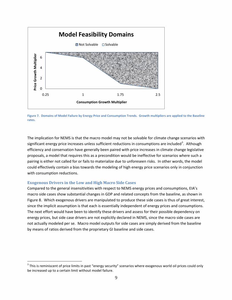
Model Feasibility Domains An interesting observation in the sensitivity studies was that the feasibility of arbitrary price increases depended upon simultaneous reductions in consumptions when NEMS derived consumption overwrites were included and held constant. Consumption overwrites effectively disable the GI model’s internal reaction functions, or elasticities of consumptions with respect to prices. In the NEMS implementation of the GI macro model, these reaction functions are replaced by elasticities of demands with respect to prices in the various NEMS demand models. In the sensitivity studies reported herein, these reaction functions were also disabled in that consumption overwrites were specified exogenously so that they could be varied independently from energy prices. Without consumption reductions, energy price increases beyond a certain point resulted in model crashing due to mathematical infeasibilities. This could be a reflection of limitations on energy expenditures, as a fraction of total expenditures, since energy consumptions beyond a certain point also were not solvable without offsetting reductions in energy prices, as shown in Figure 72

2 This is analogous to how a consumer could rebound from higher gasoline prices without changes in driving habits as long as expenditures could be kept constant by higher mileage efficiency.

. “Failures-to-solve” for an econometric model could be indicative of a scenario which is outside the bounds of the data upon which the model’s correlations and coefficients are based. Although not entirely satisfactory from a modeling viewpoint, a “failure-to-solve” could be an outcome with significant implications, especially for scenarios that are beyond business as usual, such as climate and energy security scenarios with energy prices that are high by historical standards.

9

Figure 7. Domains of Model Failure by Energy Price and Consumption Trends. Growth multipliers are applied to the Baseline rates.

The implication for NEMS is that the macro model may not be solvable for climate change scenarios with significant energy price increases unless sufficient reductions in consumptions are included3

Exogenous Drivers in the Low and High Macro Side Cases

. Although efficiency and conservation have generally been paired with price increases in climate change legislative proposals, a model that requires this as a precondition would be ineffective for scenarios where such a pairing is either not called for or fails to materialize due to unforeseen risks. In other words, the model could effectively contain a bias towards the modeling of high energy price scenarios only in conjunction with consumption reductions.

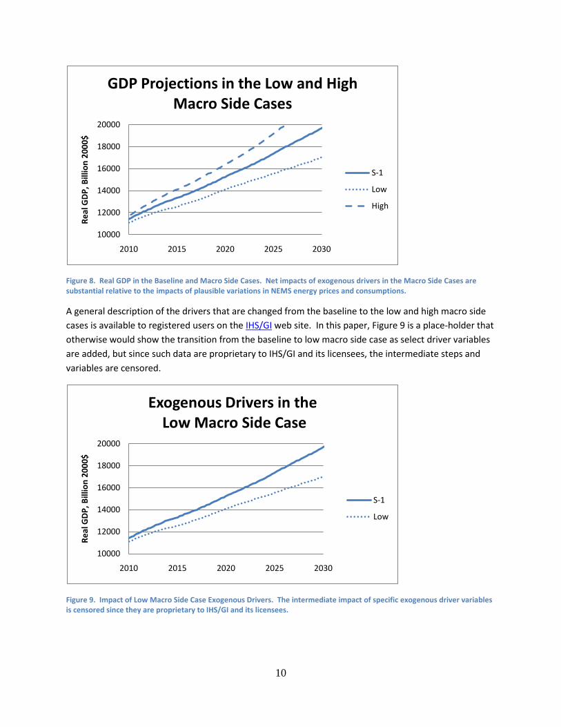
Compared to the general insensitivities with respect to NEMS energy prices and consumptions, EIA’s macro side cases show substantial changes in GDP and related concepts from the baseline, as shown in Figure 8. Which exogenous drivers are manipulated to produce these side cases is thus of great interest, since the implicit assumption is that each is essentially independent of energy prices and consumptions. The next effort would have been to identify these drivers and assess for their possible dependency on energy prices, but side case drivers are not explicitly declared in NEMS, since the macro side cases are not actually modeled per se. Macro model outputs for side cases are simply derived from the baseline by means of ratios derived from the proprietary GI baseline and side cases.

3 This is reminiscent of price limits in past “energy security” scenarios where exogenous world oil prices could only be increased up to a certain limit without model failure.

0

2

4

6

2.51.7510.25

Pric

e G

row

th M

ulti

plie

r

Consumption Growth Multiplier

Model Feasibility DomainsNot Solvable Solvable

10

Figure 8. Real GDP in the Baseline and Macro Side Cases. Net impacts of exogenous drivers in the Macro Side Cases are substantial relative to the impacts of plausible variations in NEMS energy prices and consumptions.

A general description of the drivers that are changed from the baseline to the low and high macro side cases is available to registered users on the IHS/GI web site. In this paper, Figure 9 is a place-holder that otherwise would show the transition from the baseline to low macro side case as select driver variables are added, but since such data are proprietary to IHS/GI and its licensees, the intermediate steps and variables are censored.

Figure 9. Impact of Low Macro Side Case Exogenous Drivers. The intermediate impact of specific exogenous driver variables is censored since they are proprietary to IHS/GI and its licensees.

10000

12000

14000

16000

18000

20000

2010 2015 2020 2025 2030

Real

GD

P, B

illio

n 20

00$

GDP Projections in the Low and High Macro Side Cases

S-1

Low

High

10000

12000

14000

16000

18000

20000

2010 2015 2020 2025 2030

Real

GD

P, B

illio

n 20

00$

Exogenous Drivers in theLow Macro Side Case

S-1

Low

11

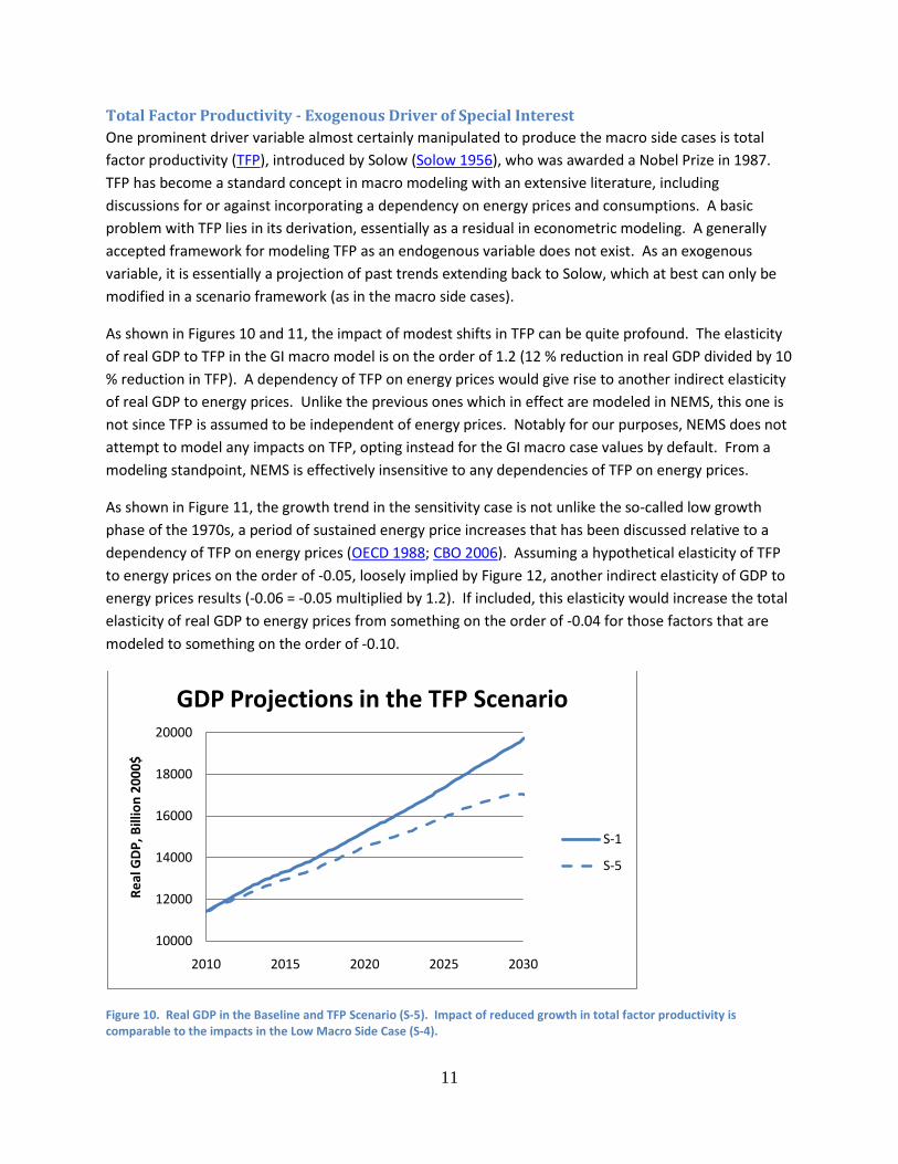
Total Factor Productivity - Exogenous Driver of Special Interest One prominent driver variable almost certainly manipulated to produce the macro side cases is total factor productivity (TFP), introduced by Solow (Solow 1956), who was awarded a Nobel Prize in 1987. TFP has become a standard concept in macro modeling with an extensive literature, including discussions for or against incorporating a dependency on energy prices and consumptions. A basic problem with TFP lies in its derivation, essentially as a residual in econometric modeling. A generally accepted framework for modeling TFP as an endogenous variable does not exist. As an exogenous variable, it is essentially a projection of past trends extending back to Solow, which at best can only be modified in a scenario framework (as in the macro side cases).

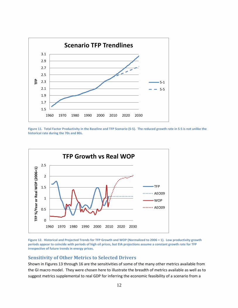
As shown in Figures 10 and 11, the impact of modest shifts in TFP can be quite profound. The elasticity of real GDP to TFP in the GI macro model is on the order of 1.2 (12 % reduction in real GDP divided by 10 % reduction in TFP). A dependency of TFP on energy prices would give rise to another indirect elasticity of real GDP to energy prices. Unlike the previous ones which in effect are modeled in NEMS, this one is not since TFP is assumed to be independent of energy prices. Notably for our purposes, NEMS does not attempt to model any impacts on TFP, opting instead for the GI macro case values by default. From a modeling standpoint, NEMS is effectively insensitive to any dependencies of TFP on energy prices.

As shown in Figure 11, the growth trend in the sensitivity case is not unlike the so-called low growth phase of the 1970s, a period of sustained energy price increases that has been discussed relative to a dependency of TFP on energy prices (OECD 1988; CBO 2006). Assuming a hypothetical elasticity of TFP to energy prices on the order of -0.05, loosely implied by Figure 12, another indirect elasticity of GDP to energy prices results (-0.06 = -0.05 multiplied by 1.2). If included, this elasticity would increase the total elasticity of real GDP to energy prices from something on the order of -0.04 for those factors that are modeled to something on the order of -0.10.

Figure 10. Real GDP in the Baseline and TFP Scenario (S-5). Impact of reduced growth in total factor productivity is comparable to the impacts in the Low Macro Side Case (S-4).

10000

12000

14000

16000

18000

20000

2010 2015 2020 2025 2030

Real

GD

P, B

illio

n 20

00$

GDP Projections in the TFP Scenario

S-1

S-5

12

Figure 11. Total Factor Productivity in the Baseline and TFP Scenario (S-5). The reduced growth rate in S-5 is not unlike the historical rate during the 70s and 80s.

Figure 12. Historical and Projected Trends for TFP Growth and WOP (Normalized to 2006 = 1). Low productivity growth periods appear to coincide with periods of high oil prices, but EIA projections assume a constant growth rate for TFP irrespective of future trends in energy prices.

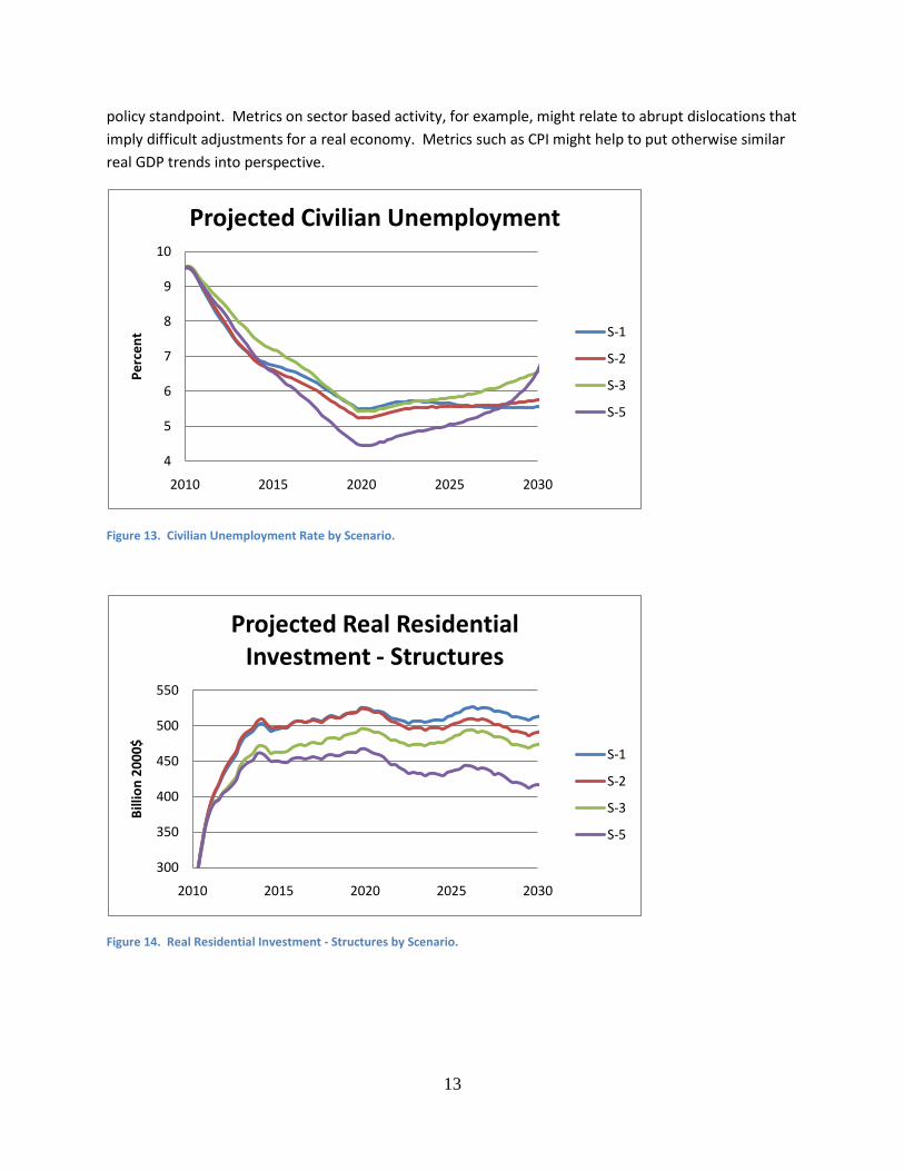
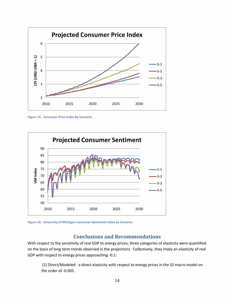
Sensitivity of Other Metrics to Selected Drivers Shown in Figures 13 through 16 are the sensitivities of some of the many other metrics available from the GI macro model. They were chosen here to illustrate the breadth of metrics available as well as to suggest metrics supplemental to real GDP for inferring the economic feasibility of a scenario from a

1.5

1.7

1.9

2.1

2.3

2.5

2.7

2.9

3.1

1960 1970 1980 1990 2000 2010 2020 2030

TFP

Scenario TFP Trendlines

S-1

S-5

0

0.5

1

1.5

2

2.5

1960 1970 1980 1990 2000 2010 2020 2030

TFP

%/Y

ear

or R

eal W

OP

(200

6=1)

TFP Growth vs Real WOP

TFP

AEO09

WOP

AEO09

13

policy standpoint. Metrics on sector based activity, for example, might relate to abrupt dislocations that imply difficult adjustments for a real economy. Metrics such as CPI might help to put otherwise similar real GDP trends into perspective.

Figure 13. Civilian Unemployment Rate by Scenario.

Figure 14. Real Residential Investment - Structures by Scenario.

4

5

6

7

8

9

10

2010 2015 2020 2025 2030

Perc

ent

Projected Civilian Unemployment

S-1

S-2

S-3

S-5

300

350

400

450

500

550

2010 2015 2020 2025 2030

Billi

on 2

000$

Projected Real Residential Investment - Structures

S-1

S-2

S-3

S-5

14

Figure 15. Consumer Price Index by Scenario.

Figure 16. University of Michigan Consumer Sentiment Index by Scenario.

Conclusions and Recommendations With respect to the sensitivity of real GDP to energy prices, three categories of elasticity were quantified on the basis of long term trends observed in the projections. Collectively, they imply an elasticity of real GDP with respect to energy prices approaching -0.1:

(1) Direct/Modeled - a direct elasticity with respect to energy prices in the GI macro model on the order of -0.005.

2

3

4

5

6

2010 2015 2020 2025 2030

CPI (

1982

-198

4 =

1)Projected Consumer Price Index

S-1

S-2

S-3

S-5

50

55

60

65

70

75

80

85

90

2010 2015 2020 2025 2030

UM

Inde

x

Projected Consumer Sentiment

S-1

S-2

S-3

S-5

15

(2) Indirect/Modeled - an indirect elasticity on the order of -0.033, marginally consistent with energy expenditures running about 10 % as a direct component of GDP (IER 2010). This elasticity is comprised of a direct elasticity of real GDP with respect to consumptions on the order of 0.33 in the GI macro model, and an elasticity of consumptions with respect to prices, assumed to be on the order of -0.10 in the NEMS supply and demand models.

(3) Indirect/Not Modeled - an indirect elasticity not currently modeled in NEMS, on the order of -0.06. This elasticity is comprised of a direct elasticity of real GDP with respect to total factor productivity on the order of 1.2 in the GI macro model, and an elasticity of total factor productivity with respect to prices on the order of -0.05, assumed on the basis of preliminary data.

The implementation of the GI macro model in NEMS disables the GI macro model’s internal reaction functions governing how energy consumptions respond to energy prices. These reaction functions are overwritten by those in the NEMS demand models. In the sensitivity studies described herein, these reaction functions were also effectively disabled so that energy price and consumption trends could be varied independently. In doing so, it was possible to map out a model feasibility domain with regard to solvability of the GI macro model. With respect to reductions in energy consumptions, the GI macro model was tolerant (no “failures-to-solve”), but with respect to energy price increases, the model was only conditionally tolerant, ultimately requiring a pairing with consumption reductions for energy price increases beyond a certain point. In all cases where the model could be solved, the direct sensitivity of real GDP to energy prices was quite small. The “failure-to-solve” for energy price increases beyond a certain point without consumption reductions presents a potential modeling bias for consumption reductions when NEMS is applied to high energy price scenarios outside the scope of the historical (business as usual) data upon which the model is based. The limits to relaxing assumptions related to consumptions in EIA’s climate change scenarios is thus of immediate interest. Since consumptions are exogenous in the NEMS implementation of the GI macro model, the realism of assumptions concerning efficiency- and conservation-driven reductions cannot be inferred because the macro model solved, or solved with minor impacts to metrics like real GDP. Direct assessment of the underlying assumptions in the demand models of NEMS would be necessary.

Total factor productivity is one exogenous driver variable in the GI macro model that has a potentially significant dependency on energy prices. The NEMS implementation of the GI macro model assumes that such a dependency does not exist. TFP exerts a profound impact on real GDP and many other metrics. The dependency of TFP and other exogenous drivers on energy prices provides a systematic framework for assessing the use of NEMS as a tool to model the viability of high energy price scenarios such as those related to climate change and energy security. Other macroeconomic models should be reviewed with respect to TFP modeling. One model in the public domain is the Fair model, which may be incorporated into the hybrid econometric input-output model being developed by the Regional Research Institute at the West Virginia University (Jackson, Rey, and Kahsai 2010). Evidence for a dependency of TFP on energy prices should also be reviewed, and if warranted, a model crafted and tested in NEMS. Generally such a model would overlay deviations onto a long term trend of TFP based upon energy price movements.

16

The GI macro model offers a wealth of metrics beyond real GDP (1,727 endogenous outputs) that could be useful for inferring the feasibility of scenarios from an economic policy standpoint. Some relate to the abruptness of transitions in sector activities, such as employment, while others such as CPI relate to the overall well-being of consumers.

17

References Blanchard, O., and Gali, J. (2007), “The Macroeconomic Effects of Oil Price Shocks - Why are the 2000s So Different from the 1970s?” August 18. CBO (2006), “The Economic Effects of Recent Increases in Energy Prices,” Congressional Budget Office Report, July, Chapter 2, page 11.

EIA (2010), “Model Documentation Report - Macroeconomic Activity Module (MAM) of the National Energy Modeling System,” DOE/EIA-M065(2010), May.

Geisbrecht, R. (2009), “Extending the CCS Retrofit Market by Refurbishing Coal Fired Power Plants - Simulations with the National Energy Modeling System,” DOE/NETL-2009/1374, July 31. IER (2010), “A Primer on Energy and the Economy: Energy’s Large Share of the Economy Requires Caution in Determining Policies That Affect It,” February 16. Jackson, R., Rey, S., and Kahsai, M. S. (2010), “Forecasting Economic and Employment Impacts of NETL Programs through an Econometric Input-Output Model, Phase II: Model Design,” June. Klara, J. (2006), “Office of Fossil Energy Programs - Inputs for FY2006 Benefits Estimates,” November. NRC (2007), “Prospective Evaluation of Applied Energy Research and Development at DOE - Phase Two,” The National Academies Press, Washington D.C. OECD (1988), “Total Factor Productivity - Macroeconomic and Structural Aspects of the Slowdown,” OECD Economic Studies No. 10 (A. Steven Englander and Axel Mittelstädt), May 17. Peace, J., and Weyant J. (2008), “Insights Not Numbers - The Appropriate Use of Economic Models,” Pew Center on Global Climate Change, April. Roubini, N., and Setzer, B. (2004), “The Effects of the Recent Oil Price Shock on the U.S. and Global Economy,” August. Solow, R. (1956), “A Contribution to the Theory of Economic Growth,” Quarterly Journal of Economics Vol. 70, No. 1, February, pages 65-94.

18

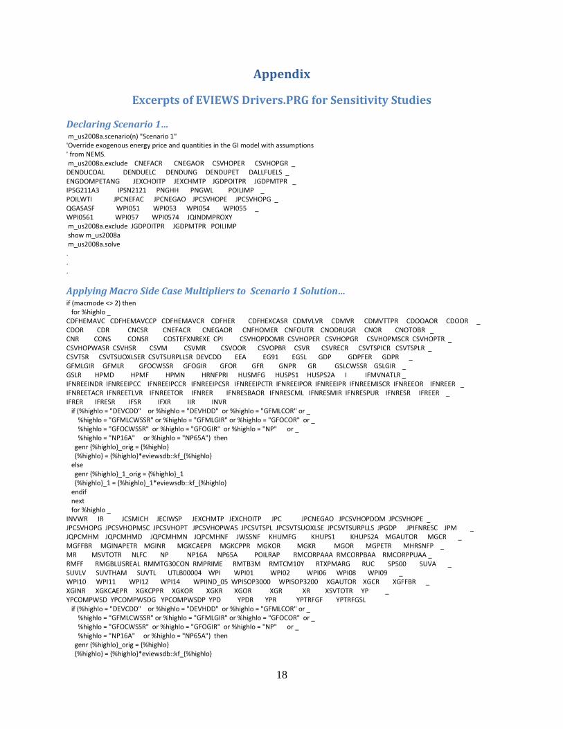
Appendix

Excerpts of EVIEWS Drivers.PRG for Sensitivity Studies

Declaring Scenario 1… m_us2008a.scenario(n) "Scenario 1" 'Override exogenous energy price and quantities in the GI model with assumptions ' from NEMS. m_us2008a.exclude CNEFACR CNEGAOR CSVHOPER CSVHOPGR _ DENDUCOAL DENDUELC DENDUNG DENDUPET DALLFUELS _ ENGDOMPETANG JEXCHOITP JEXCHMTP JGDPOITPR JGDPMTPR _ IPSG211A3 IPSN2121 PNGHH PNGWL POILIMP _ POILWTI JPCNEFAC JPCNEGAO JPCSVHOPE JPCSVHOPG _ QGASASF WPI051 WPI053 WPI054 WPI055 _ WPI0561 WPI057 WPI0574 JQINDMPROXY m_us2008a.exclude JGDPOITPR JGDPMTPR POILIMP show m_us2008a m_us2008a.solve . . .

Applying Macro Side Case Multipliers to Scenario 1 Solution…

if (macmode <> 2) then for %highlo _ CDFHEMAVC CDFHEMAVCCP CDFHEMAVCR CDFHER CDFHEXCASR CDMVLVR CDMVR CDMVTTPR CDOOAOR CDOOR _ CDOR CDR CNCSR CNEFACR CNEGAOR CNFHOMER CNFOUTR CNODRUGR CNOR CNOTOBR _ CNR CONS CONSR COSTEFXNREXE CPI CSVHOPDOMR CSVHOPER CSVHOPGR CSVHOPMSCR CSVHOPTR _ CSVHOPWASR CSVHSR CSVM CSVMR CSVOOR CSVOPBR CSVR CSVRECR CSVTSPICR CSVTSPLR _ CSVTSR CSVTSUOXLSER CSVTSURPLLSR DEVCDD EEA EG91 EGSL GDP GDPFER GDPR _ GFMLGIR GFMLR GFOCWSSR GFOGIR GFOR GFR GNPR GR GSLCWSSR GSLGIR _ GSLR HPMD HPMF HPMN HRNFPRI HUSMFG HUSPS1 HUSPS2A I IFMVNATLR _ IFNREEINDR IFNREEIPCC IFNREEIPCCR IFNREEIPCSR IFNREEIPCTR IFNREEIPOR IFNREEIPR IFNREEMISCR IFNREEOR IFNREER _ IFNREETACR IFNREETLVR IFNREETOR IFNRER IFNRESBAOR IFNRESCML IFNRESMIR IFNRESPUR IFNRESR IFREER _ IFRER IFRESR IFSR IFXR IIR INVR if (%highlo = "DEVCDD" or %highlo = "DEVHDD" or %highlo = "GFMLCOR" or _ %highlo = "GFMLCWSSR" or %highlo = "GFMLGIR" or %highlo = "GFOCOR" or _ %highlo = "GFOCWSSR" or %highlo = "GFOGIR" or %highlo = "NP" or _ %highlo = "NP16A" or %highlo = "NP65A") then genr {%highlo}_orig = {%highlo} {%highlo} = {%highlo}*eviewsdb::kf_{%highlo} else genr {%highlo}_1_orig = {%highlo}_1 {%highlo}_1 = {%highlo}_1*eviewsdb::kf_{%highlo} endif next for %highlo _ INVWR IR JCSMICH JECIWSP JEXCHMTP JEXCHOITP JPC JPCNEGAO JPCSVHOPDOM JPCSVHOPE _ JPCSVHOPG JPCSVHOPMSC JPCSVHOPT JPCSVHOPWAS JPCSVTSPL JPCSVTSUOXLSE JPCSVTSURPLLS JPGDP JPIFNRESC JPM _ JQPCMHM JQPCMHMD JQPCMHMN JQPCMHNF JWSSNF KHUMFG KHUPS1 KHUPS2A MGAUTOR MGCR _ MGFFBR MGINAPETR MGINR MGKCAEPR MGKCPPR MGKOR MGKR MGOR MGPETR MHRSNFP _ MR MSVTOTR NLFC NP NP16A NP65A POILRAP RMCORPAAA RMCORPBAA RMCORPPUAA _ RMFF RMGBLUSREAL RMMTG30CON RMPRIME RMTB3M RMTCM10Y RTXPMARG RUC SP500 SUVA _ SUVLV SUVTHAM SUVTL UTLB00004 WPI WPI01 WPI02 WPI06 WPI08 WPI09 _ WPI10 WPI11 WPI12 WPI14 WPIIND_05 WPISOP3000 WPISOP3200 XGAUTOR XGCR XGFFBR _ XGINR XGKCAEPR XGKCPPR XGKOR XGKR XGOR XGR XR XSVTOTR YP _ YPCOMPWSD YPCOMPWSDG YPCOMPWSDP YPD YPDR YPR YPTRFGF YPTRFGSL if (%highlo = "DEVCDD" or %highlo = "DEVHDD" or %highlo = "GFMLCOR" or _ %highlo = "GFMLCWSSR" or %highlo = "GFMLGIR" or %highlo = "GFOCOR" or _ %highlo = "GFOCWSSR" or %highlo = "GFOGIR" or %highlo = "NP" or _ %highlo = "NP16A" or %highlo = "NP65A") then genr {%highlo}_orig = {%highlo} {%highlo} = {%highlo}*eviewsdb::kf_{%highlo}

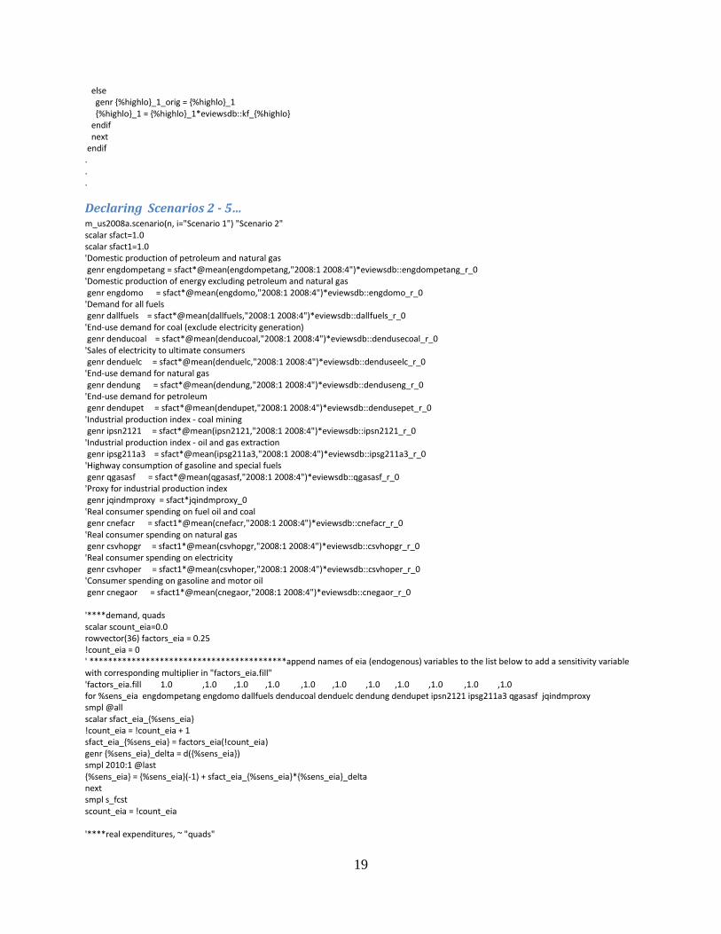
19

else genr {%highlo}_1_orig = {%highlo}_1 {%highlo}_1 = {%highlo}_1*eviewsdb::kf_{%highlo} endif next endif . . .

Declaring Scenarios 2 - 5…

m_us2008a.scenario(n, i="Scenario 1") "Scenario 2" scalar sfact=1.0 scalar sfact1=1.0 'Domestic production of petroleum and natural gas genr engdompetang = sfact*@mean(engdompetang,"2008:1 2008:4")*eviewsdb::engdompetang_r_0 'Domestic production of energy excluding petroleum and natural gas genr engdomo = sfact*@mean(engdomo,"2008:1 2008:4")*eviewsdb::engdomo_r_0 'Demand for all fuels genr dallfuels = sfact*@mean(dallfuels,"2008:1 2008:4")*eviewsdb::dallfuels_r_0 'End-use demand for coal (exclude electricity generation) genr denducoal = sfact*@mean(denducoal,"2008:1 2008:4")*eviewsdb::dendusecoal_r_0 'Sales of electricity to ultimate consumers genr denduelc = sfact*@mean(denduelc,"2008:1 2008:4")*eviewsdb::denduseelc_r_0 'End-use demand for natural gas genr dendung = sfact*@mean(dendung,"2008:1 2008:4")*eviewsdb::denduseng_r_0 'End-use demand for petroleum genr dendupet = sfact*@mean(dendupet,"2008:1 2008:4")*eviewsdb::dendusepet_r_0 'Industrial production index - coal mining genr ipsn2121 = sfact*@mean(ipsn2121,"2008:1 2008:4")*eviewsdb::ipsn2121_r_0 'Industrial production index - oil and gas extraction genr ipsg211a3 = sfact*@mean(ipsg211a3,"2008:1 2008:4")*eviewsdb::ipsg211a3_r_0 'Highway consumption of gasoline and special fuels genr qgasasf = sfact*@mean(qgasasf,"2008:1 2008:4")*eviewsdb::qgasasf_r_0 'Proxy for industrial production index genr jqindmproxy = sfact*jqindmproxy_0 'Real consumer spending on fuel oil and coal genr cnefacr = sfact1*@mean(cnefacr,"2008:1 2008:4")*eviewsdb::cnefacr_r_0 'Real consumer spending on natural gas genr csvhopgr = sfact1*@mean(csvhopgr,"2008:1 2008:4")*eviewsdb::csvhopgr_r_0 'Real consumer spending on electricity genr csvhoper = sfact1*@mean(csvhoper,"2008:1 2008:4")*eviewsdb::csvhoper_r_0 'Consumer spending on gasoline and motor oil genr cnegaor = sfact1*@mean(cnegaor,"2008:1 2008:4")*eviewsdb::cnegaor_r_0 '****demand, quads scalar scount_eia=0.0 rowvector(36) factors_eia = 0.25 !count_eia = 0 ' ******************************************append names of eia (endogenous) variables to the list below to add a sensitivity variable with corresponding multiplier in "factors_eia.fill" 'factors_eia.fill 1.0 ,1.0 ,1.0 ,1.0 ,1.0 ,1.0 ,1.0 ,1.0 ,1.0 ,1.0 ,1.0 for %sens_eia engdompetang engdomo dallfuels denducoal denduelc dendung dendupet ipsn2121 ipsg211a3 qgasasf jqindmproxy smpl @all scalar sfact_eia_{%sens_eia} !count_eia = !count_eia + 1 sfact_eia_{%sens_eia} = factors_eia(!count_eia) genr {%sens_eia}_delta = d({%sens_eia}) smpl 2010:1 @last {%sens_eia} = {%sens_eia}(-1) + sfact_eia_{%sens_eia}*{%sens_eia}_delta next smpl s_fcst scount_eia = !count_eia '****real expenditures, ~ "quads"

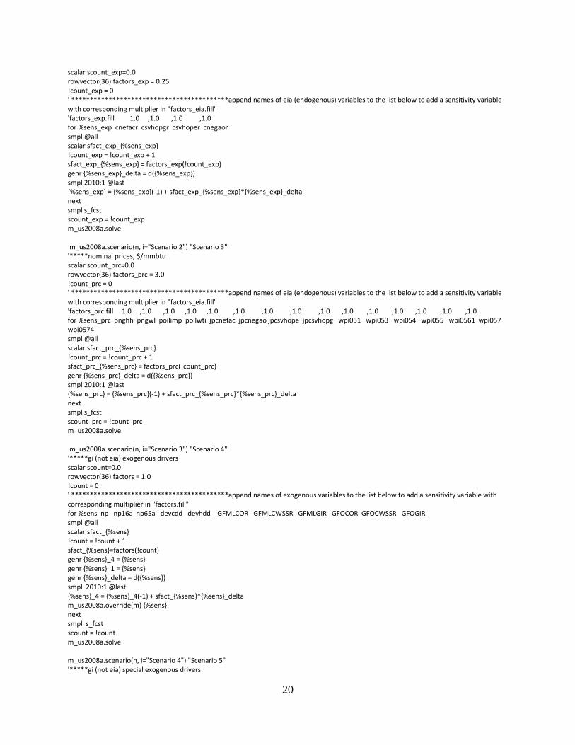
20

scalar scount_exp=0.0 rowvector(36) factors_exp = 0.25 !count_exp = 0 ' ******************************************append names of eia (endogenous) variables to the list below to add a sensitivity variable with corresponding multiplier in "factors_eia.fill" 'factors_exp.fill 1.0 ,1.0 ,1.0 ,1.0 for %sens_exp cnefacr csvhopgr csvhoper cnegaor smpl @all scalar sfact_exp_{%sens_exp} !count_exp = !count_exp + 1 sfact_exp_{%sens_exp} = factors_exp(!count_exp) genr {%sens_exp}_delta = d({%sens_exp}) smpl 2010:1 @last {%sens_exp} = {%sens_exp}(-1) + sfact_exp_{%sens_exp}*{%sens_exp}_delta next smpl s_fcst scount_exp = !count_exp m_us2008a.solve m_us2008a.scenario(n, i="Scenario 2") "Scenario 3" '*****nominal prices, $/mmbtu scalar scount_prc=0.0 rowvector(36) factors_prc = 3.0 !count_prc = 0 ' ******************************************append names of eia (endogenous) variables to the list below to add a sensitivity variable with corresponding multiplier in "factors_eia.fill" 'factors_prc.fill 1.0 ,1.0 ,1.0 ,1.0 ,1.0 ,1.0 ,1.0 ,1.0 ,1.0 ,1.0 ,1.0 ,1.0 ,1.0 ,1.0 ,1.0 for %sens_prc pnghh pngwl poilimp poilwti jpcnefac jpcnegao jpcsvhope jpcsvhopg wpi051 wpi053 wpi054 wpi055 wpi0561 wpi057 wpi0574 smpl @all scalar sfact_prc_{%sens_prc} !count_prc = !count_prc + 1 sfact_prc_{%sens_prc} = factors_prc(!count_prc) genr {%sens_prc}_delta = d({%sens_prc}) smpl 2010:1 @last {%sens_prc} = {%sens_prc}(-1) + sfact_prc_{%sens_prc}*{%sens_prc}_delta next smpl s_fcst scount_prc = !count_prc m_us2008a.solve m_us2008a.scenario(n, i="Scenario 3") "Scenario 4" '*****gi (not eia) exogenous drivers scalar scount=0.0 rowvector(36) factors = 1.0 !count = 0 ' ******************************************append names of exogenous variables to the list below to add a sensitivity variable with corresponding multiplier in "factors.fill" for %sens np np16a np65a devcdd devhdd GFMLCOR GFMLCWSSR GFMLGIR GFOCOR GFOCWSSR GFOGIR smpl @all scalar sfact_{%sens} !count = !count + 1 sfact_{%sens}=factors(!count) genr {%sens}_4 = {%sens} genr {%sens}_1 = {%sens} genr {%sens}_delta = d({%sens}) smpl 2010:1 @last {%sens}_4 = {%sens}_4(-1) + sfact_{%sens}*{%sens}_delta m_us2008a.override(m) {%sens} next smpl s_fcst scount = !count m_us2008a.solve m_us2008a.scenario(n, i="Scenario 4") "Scenario 5" '*****gi (not eia) special exogenous drivers

21

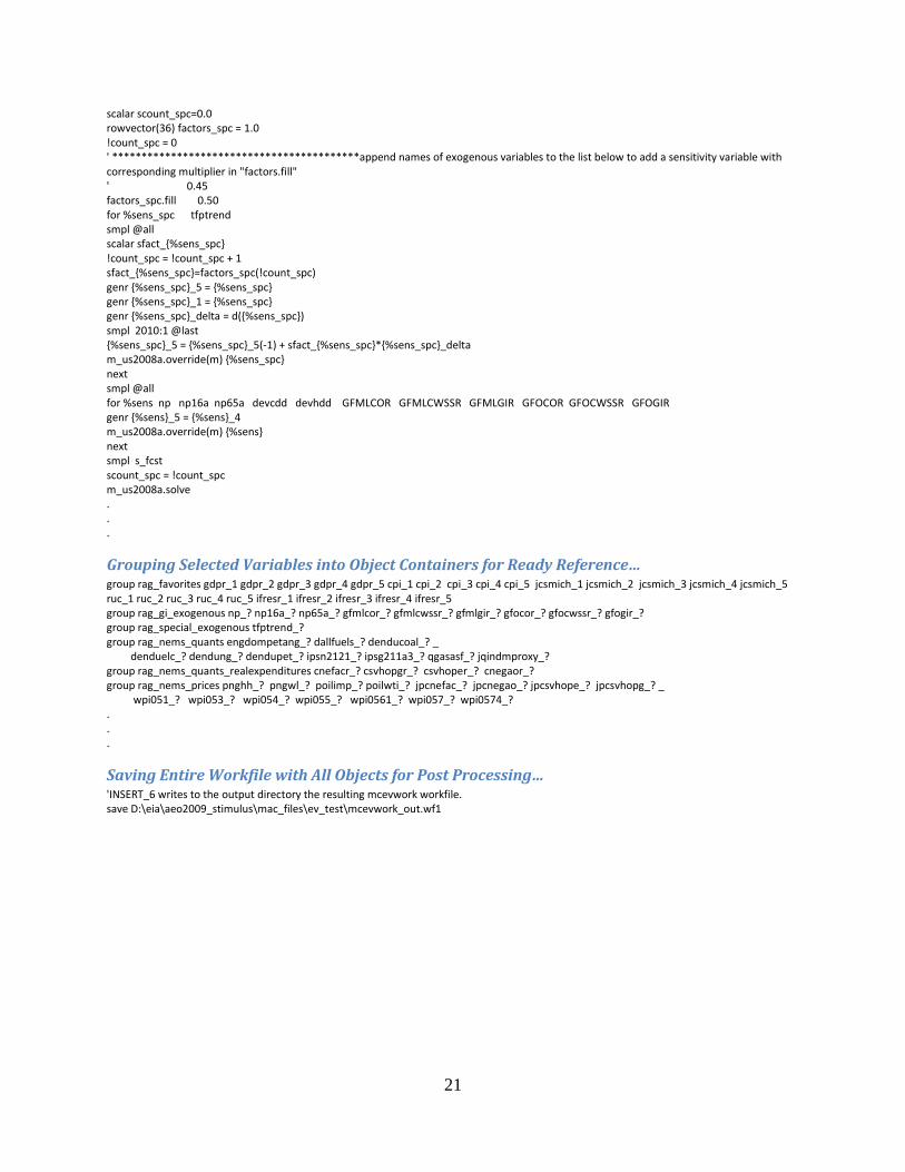
scalar scount_spc=0.0 rowvector(36) factors_spc = 1.0 !count_spc = 0 ' ******************************************append names of exogenous variables to the list below to add a sensitivity variable with corresponding multiplier in "factors.fill" ' 0.45 factors_spc.fill 0.50 for %sens_spc tfptrend smpl @all scalar sfact_{%sens_spc} !count_spc = !count_spc + 1 sfact_{%sens_spc}=factors_spc(!count_spc) genr {%sens_spc}_5 = {%sens_spc} genr {%sens_spc}_1 = {%sens_spc} genr {%sens_spc}_delta = d({%sens_spc}) smpl 2010:1 @last {%sens_spc}_5 = {%sens_spc}_5(-1) + sfact_{%sens_spc}*{%sens_spc}_delta m_us2008a.override(m) {%sens_spc} next smpl @all for %sens np np16a np65a devcdd devhdd GFMLCOR GFMLCWSSR GFMLGIR GFOCOR GFOCWSSR GFOGIR genr {%sens}_5 = {%sens}_4 m_us2008a.override(m) {%sens} next smpl s_fcst scount_spc = !count_spc m_us2008a.solve . . .

Grouping Selected Variables into Object Containers for Ready Reference… group rag_favorites gdpr_1 gdpr_2 gdpr_3 gdpr_4 gdpr_5 cpi_1 cpi_2 cpi_3 cpi_4 cpi_5 jcsmich_1 jcsmich_2 jcsmich_3 jcsmich_4 jcsmich_5 ruc_1 ruc_2 ruc_3 ruc_4 ruc_5 ifresr_1 ifresr_2 ifresr_3 ifresr_4 ifresr_5 group rag_gi_exogenous np_? np16a_? np65a_? gfmlcor_? gfmlcwssr_? gfmlgir_? gfocor_? gfocwssr_? gfogir_? group rag_special_exogenous tfptrend_? group rag_nems_quants engdompetang_? dallfuels_? denducoal_? _ denduelc_? dendung_? dendupet_? ipsn2121_? ipsg211a3_? qgasasf_? jqindmproxy_? group rag_nems_quants_realexpenditures cnefacr_? csvhopgr_? csvhoper_? cnegaor_? group rag_nems_prices pnghh_? pngwl_? poilimp_? poilwti_? jpcnefac_? jpcnegao_? jpcsvhope_? jpcsvhopg_? _ wpi051_? wpi053_? wpi054_? wpi055_? wpi0561_? wpi057_? wpi0574_? . . .

Saving Entire Workfile with All Objects for Post Processing… 'INSERT_6 writes to the output directory the resulting mcevwork workfile. save D:\eia\aeo2009_stimulus\mac_files\ev_test\mcevwork_out.wf1