CLIMATE RESEARCHClim Res

Vol. 23: 233–246, 2003 Published April 10

1. INTRODUCTION

Understanding how climate changes impact waterresources is a task of utmost importance. The increasein temperature during the 20th century is well docu-mented on a global and regional scale (IPCC 2001).Changes in several climate parameters related to thehydrological cycle have also been detected during thelast few decades. Across Europe, an increase in themean precipitation amount (e.g. Schönwiese & Rapp1997, Osborn et al. 2000) and in heavy and extremeprecipitation events (Gellens 2000, Osborn et al. 2000,Frei & Schär 2001) in the cold season, a reduction insnow cover in spring (Robinson 1997, Brown 2000) and

a retreat of the Alpine glaciers (Oerlemans 1994, IPCC2001) have been revealed. Some evidence emergesthat changes in climate have already resulted in anincreasing frequency of floods of a number of majorrivers (Groisman et al. 2001, Milly et al. 2002).

Continuous warming is the most consistent resultamong all the general-circulation-model (GCM) inte-grations of future climate, both globally and overEurope. Model integrations also suggest a continuingupward trend in winter precipitation in mid- and high-latitude Europe, a downward trend in summer precip-itation in southern Europe (IPCC 2001), and a furtherretreat of European glaciers (Schneeberger et al.2001). Changes in precipitation extrema, such as an

© Inter-Research 2003 · www.int-res.com*Corresponding author. Email: adri.buishand@knmi.nl

Assessing future discharge of the river Rhineusing regional climate model integrations and

a hydrological model

M. V. Shabalova1, W. P. A. van Deursen2, T. A. Buishand1,*

1Royal Netherlands Meteorological Institute (KNMI), PO Box 201, 3730 AE De Bilt, The Netherlands2Carthago Consultancy, Oostzeedijk Beneden 23a, 3062 VK Rotterdam, The Netherlands

ABSTRACT: Climate change scenarios based on integrations of the Hadley Centre regional climatemodel HadRM2 are used to determine the change in the flow regime of the river Rhine by the end ofthe 21st century. Two scenarios are formulated: Scenario 1 accounting for the temperature increase(4.8°C on average over the basin) and changes in the mean precipitation, and Scenario 2 accountingadditionally for changes in the temperature variance and an increase in the relative variability of pre-cipitation. These scenarios are used as input into the RhineFlow hydrological model, a distributedwater balance model of the Rhine basin that simulates river flow, soil moisture, snow pack andgroundwater storage with a 10 d time step. Both scenarios result in higher mean discharges of theRhine in winter (approx. +30%), but lower mean discharges in summer (approx. –30%), particularlyin August (approx. –50%). RhineFlow simulations also indicate that the variability of the 10 d dis-charges increases significantly, even if the variability of the climatic inputs remains unchanged. Theannual maximum discharge increases in magnitude throughout the Rhine and tends to occur morefrequently in winter, thus suggesting an increasing risk of winter floods. This is especially pro-nounced in Scenario 2. At the Netherlands-German border, the magnitude of the 20 yr maximum dis-charge event increases by 14% in Scenario 1 and by 29% in Scenario 2; the present-day 20 yr eventtends to reappear every 5 yr in Scenario 1 and every 3 yr in Scenario 2. The frequency of occurrenceof low and very low flows increases, in both scenarios alike.

KEY WORDS: Climate change impact · Regional climate model · Climate change scenarios · Rhinedischarge · Extreme river flows

Resale or republication not permitted without written consent of the publisher

Clim Res 23: 233–246, 2003

increase in the precipitation intensity, the proportion ofheavy rains, and the occurrence of very wet seasonsare also projected for the future (e.g. Frei et al. 1998,Meehl et al. 2000, Jones & Reid 2001, Räisänen &Joelsson 2001, Palmer & Räisänen 2002). Assessmentsof the impact of climate changes on river flows are inprogress (e.g. Arpe & Roeckner 1999, Bergström et al.2001, Milly et al. 2002).

The Rhine is the longest river in Western Europe(basin 185 000 km2) stretching from the Swiss Alps tothe Dutch coast of the North Sea (Fig. 1). Its water isused for domestic consumption, irrigation, hydropowerindustry and prevention of salt-water intrusion fromthe North Sea in polder areas. The navigation on theRhine is intense. Climate-related changes in streamflow and water availability will affect all these river-related activities.

It is therefore not surprising that, especially in TheNetherlands, a number of projects were devoted toassessments of climate change impacts on the hydro-logy of the Rhine (Kwadijk 1993, Grabs 1997, Middel-koop 2000). A conceptual water balance model for theRhine basin was specifically designed to accomplishthese ends (Kwadijk 1993, van Deursen & Kwadijk1993). A tendency for an increase in winter runoff and

a decrease in summer runoff of the Rhine in simulatedfuture climates has been revealed. However, climatechange scenarios used in those studies were based onrather old runs of GCMs (from the late 1980s to early1990s) and did not account for a possible change in thevariability of climatic inputs.

The present paper investigates the effect of climatechange on the discharge of the Rhine using a recentsimulation of future climate conducted by the HadleyCentre with the regional climate model HadRM2, andan updated version of the hydrological model of theRhine. The latter is briefly described in Section 2. InSection 3, the analysis of the regional climate modeloutput is performed for the Rhine basin, with emphasison parameters that are crucial for hydrological applica-tion, such as the number of wet and very wet days,10 d maximum precipitation totals, and the variancesof temperature and precipitation. Climate change sce-narios are formulated at the end of Section 3; one ofthem accounts for changes in both the mean and vari-ability of temperature and precipitation. The results onchanges in the mean and variability of the river Rhinedischarge are given in Section 4. Section 5 concludesthe paper.

2. RHINEFLOW MODEL

2.1. Model description

The RhineFlow hydrological model is a spatially dis-tributed water balance model of the Rhine basin thatcan simulate river flow, soil moisture, snow pack andgroundwater storage with a monthly (first version) or10 d time step. With this relatively long time stephydraulic routing can be ignored. A full description ofthe RhineFlow model is given in Kwadijk (1993), vanDeursen & Kwadijk (1993), and Kwadijk & Rotmans(1995), so only a brief summary of the model is givenhere, with some detail on the recent model update.

RhineFlow uses a spatial database implemented in araster Geographical Information System. The spatialresolution is 3 × 3 km in the present study. The modelcalculates the amount of water in the water balancecompartments of the basin from meteorological data.Apart from geographical data on topography, land use,soil type and groundwater flow characteristics, thefollowing meteorological input variables are used: the10 d averages of the maximum, minimum and meantemperature, and the 10 d totals of potential evapo-transpiration and precipitation. The minimum andmaximum temperatures are used in the calculation ofsnow accumulation and snow melt. Potential evapo-transpiration is represented as the product of a cropfactor and open water evaporation, as calculated from

234

Fig. 1. Basin of the river Rhine

Shabalova et al.: Assessing future discharge of the river Rhine

meteorological data on temperature, in-coming solar radiation, relative humidityand wind speed using the Penman for-mula. The conversion of potential to actualevapotranspiration is based on Thorn-thwaite & Mather (1957).

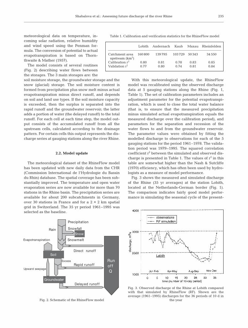
The model consists of several routines(Fig. 2) describing water flows betweenthe storages. The 3 main storages are: thesoil moisture storage, the groundwater storage and thesnow (glacial) storage. The soil moisture content isformed from precipitation plus snow melt minus actualevapotranspiration minus direct runoff, and dependson soil and land use types. If the soil moisture capacityis exceeded, then the surplus is separated into therapid runoff and the groundwater reservoir; the latteradds a portion of water (the delayed runoff) to the totalrunoff. For each cell at each time step, the model out-put consists of the accumulated runoff from all theupstream cells, calculated according to the drainagepattern. For certain cells this output represents the dis-charge series at gauging stations along the river Rhine.

2.2. Model update

The meteorological dataset of the RhineFlow modelhas been updated with new daily data from the CHR(Commission International de l’Hydrologie du Bassindu Rhin) database. The spatial coverage has been sub-stantially improved. The temperature and open waterevaporation series are now available for more than 70stations in the Rhine basin. The precipitation series areavailable for about 200 subcatchments in Germany,over 30 stations in France and for a 2 × 2 km spatialgrid in Switzerland. The 35 yr period 1961–1995 wasselected as the baseline.

With this meteorological update, the RhineFlowmodel was recalibrated using the observed dischargedata at 5 gauging stations along the Rhine (Fig. 1,Table 1). The set of calibration parameters includes anadjustment parameter for the potential evapotranspi-ration, which is used to close the total water balance(that is, to ensure that the measured precipitationminus simulated actual evapotranspiration equals themeasured discharge over the calibration period), andparameters for the separation and recession of thewater flows to and from the groundwater reservoir.The parameter values were obtained by fitting themodelled discharge to observations for each of the 5gauging stations for the period 1961–1978. The valida-tion period was 1979–1995. The squared correlationcoefficient r2 between the simulated and observed dis-charge is presented in Table 1. The values of r2 in thistable are somewhat higher than the Nash & Sutcliffe(1970) efficiency, which has often been used by hydro-logists as a measure of model performance.

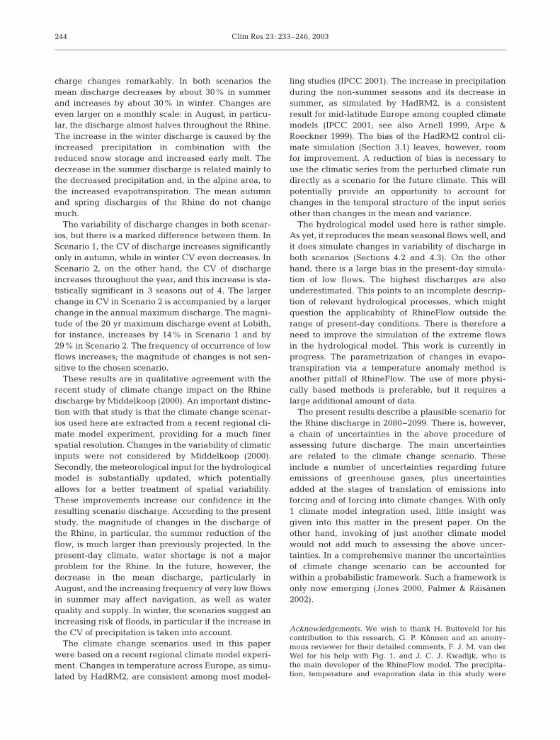
Fig. 3 shows the measured and simulated dischargeof the Rhine (35 yr averages) at the station Lobith,located at the Netherlands-German border (Fig. 1).The comparison indicates fairly good model perfor-mance in simulating the seasonal cycle of the present-

235

Soil

Groundwater

Runof f Q

Snow

Snowfall

Snowmelt

Direct unof f

Rapid r

r

unof f

Delayed runof f

Precipitation

Rain

Evapotranspiration

Upward seepage

Excess

Fig. 2. Schematic of the RhineFlow model

Table 1. Calibration and verification statistics for the RhineFlow model

Lobith Andernach Kaub Maxau Rheinfelden

Catchment area 160 800 139 795 103 729 50 343 34 550upstream (km2)

Calibration r2 0.80 0.81 0.78 0.83 0.85Validation r2 0.77 0.80 0.74 0.81 0.84

Fig. 3. Observed discharge of the Rhine at Lobith comparedwith that simulated by RhineFlow (RF). Shown are theaverage (1961–1995) discharges for the 36 periods of 10 d in

the year

Clim Res 23: 233–246, 2003

day discharge of the Rhine. Other gauging stationsalong the Rhine demonstrate a similar level of agree-ment between the observations and simulations; foreach station the annual mean is within 3% of theobserved value.

The high flows are also satisfactorily reproduced byRhineFlow. The annual maximum 10 d discharges atLobith for the 1961–1995 period, observed and simu-lated, are compared in Fig. 4a. The mean bias is small(approx. –2%); however, the highest discharges tendto be considerably underestimated. Although in theupper part of the basin the model tends to deviatemore from the observations, the mean bias is stillwithin 10% of the observed value at every gaugingstation. The low flows, on the other hand, are system-atically underestimated by RhineFlow (Fig. 4b). Al-though in absolute terms the bias in the annual minimais small and comparable in magnitude to that in the

annual maxima of the 10 d discharges, it is rather largein relative terms (26% at Lobith). A better treatment ofthe direct runoff, soil moisture budget and ground-water discharge is needed to improve the accuracy ofthe simulation of low flows.

To simulate the future discharge of the Rhine, theRhineFlow model has to be run with altered meteoro-logical inputs. Changes in temperature and precipita-tion for the future are obtained from climate modelintegrations. Changes in potential evapotranspirationare then calculated within the RhineFlow model usinga relation between the change in open water evapora-tion and temperature for The Netherlands (Brandsma1995). Possible effects of changes in incoming solarradiation, relative humidity and wind speed on evapo-transpiration are neglected.

3. CLIMATE CHANGE SCENARIOS

Temperature and precipitation changes at the end ofthe 21st century were derived from the Hadley Centreregional climate model HadRM2 nested within theglobal coupled climate model HadCM2 (Johns et al.1997). HadRM2 is a limited area model with a grid res-olution of about 50 × 50 km, driven at its boundaries byoutput from HadCM2. The finer resolution of HadRM2provides for a more realistic simulation of precipita-tion than that of HadCM2 (Noguer et al. 1998, Dur-man et al. 2001). The output from 2 integrations ofHadCM2/HadRM2 was used. The control climate sim-ulation was conducted with a constant greenhouse gasforcing representative of the second half of the 20thcentury. Thirty years of simulation were available foranalysis. The boundary conditions for the future cli-mate in HadRM2 were taken from a transient climatechange experiment with HadCM2 performed usinghistorical greenhouse gas forcing from 1860 to 1989and a 1% yr–1 increase in equivalent CO2 after this. Nosulphate aerosol forcing was included. This impliesrather large temperature changes, 3.0°C by the 2080s,similar to those resulting from the scenario IS92a(IPCC 1996). Twenty years (2080–2099) of perturbedclimate simulation with HadRM2 were available. Inthe following sections, the climate change estimateswere derived from the 20 yr perturbed run and the last20 yr of the control run. The complete control run wasused, however, in comparisons with the observedclimate.

There are 89 HadRM2 grid points in the Rhine basin.The fields of precipitation and mean, maximum andminimum temperature were extracted for the Rhinearea with daily resolution and averaged or accumu-lated over 10 d. Actual evapotranspiration data (monthlyresolution) from HadRM2 were used in checks on

236

Fig. 4. Observed annual (a) maxima and (b) minima of theRhine discharge at Lobith compared with those simulated byRhineFlow (RF). The annual maximum for a given year iscomputed for the period running from September of theprevious year to September; the annual minimum refers to

the calendar year

a

b

Shabalova et al.: Assessing future discharge of the river Rhine

the consistency of the control climate simulated byHadRM2 with observations, as well as in checks on thecalculated changes of evapotranspiration in the Rhine-Flow model.

3.1. Control climate

The differences between the HadRM2 control cli-mate simulation and the climatology (1961–1995) ofthe RhineFlow model are shown in Fig. 5 for the aver-age annual temperature and in Fig. 6 for the averagetotal annual precipitation. The cold and wet bias ofHadRM2, evident in these figures, was noted earlierby Noguer et al. (1998) for most of Europe. The Rhinebasin averaged bias relative to the RhineFlow climato-logy is –1°C for temperature and 180 mm (16%) forprecipitation. The wet bias is partly a result of the factthat the observed precipitation amounts were not cor-rected for the systematic undercatch inherent to raingauges. The bias in mean annual actual evapotranspi-ration is 56 mm (12%). As a result of these biases in theHadRM2 control climate simulation, the differencebetween the simulated values of the area-averagedprecipitation and actual evapotranspiration (577 mmyr–1) exceeds the observed mean annual discharge atLobith (449 mm yr–1) by 29%.

The bias of HadRM2 varies seasonally and is largestin winter for precipitation and in spring and summerfor temperature. It varies also spatially, being largestin the alpine region. Locally, the bias exceeds 5°C inmean annual temperature and 100% in mean annual

precipitation. On the other hand, in the low part of theRhine basin HadRM2 performs very well, even on themonthly timescale. Fig. 7 shows the observed and sim-ulated monthly averages of precipitation and actualevapotranspiration representative of the east of TheNetherlands. The values of actual evapotranspirationwere derived from measurements in the HupselseBeek experimental catchment for the period 1976–1982(Stricker 1981, de Bruin & Stricker 2000) and thevalues of precipitation from the nearby climatologicalstation Winterswijk for the period 1951–1980. The biasin both variables is typically within 20%.

In spite of bias, HadRM2 reproduces the geographi-cal structure of the observed temperature quite welland that of precipitation reasonably. The pattern cor-relation with observations is 0.54 for mean annualprecipitation and 0.95 for mean annual temperature.These values hardly change over the year: 0.52/0.46for precipitation and 0.91/0.96 for temperature inwinter/summer, respectively. The pattern correlationof the annual temperature and precipitation fields is–0.86 in HadRM2 versus –0.73 in observations.

3.2. Changes in temperature and precipitation

3.2.1. Mean fields

The perturbed minus control run values of meanannual temperature and precipitation are shown inFigs. 8 & 9, respectively. The precipitation changes are

237

Fig. 5. Difference in mean annual temperature between thecontrol climate integration of HadRM2 and the actual base-

line climatology aggregated to the HadRM2 grid

Fig. 6. Difference in total annual precipitation between thecontrol climate integration of HadRM2 and the actual base-

line climatology aggregated to the HadRM2 grid

°C

1

0

-1

-2

-3

-4

-5

-6

%

>200150100500-50-100

Clim Res 23: 233–246, 2003

expressed in percent of the control run means. Themean annual temperature increases over the wholearea, with the largest increase in the Alps. The basinaveraged warming is 5.8°C in winter and 4.7°C in sum-mer; the annual mean warming is 4.8°C. The corre-sponding change in mean annual actual evapotranspi-ration is 56 mm (+10%) on average; in winter theactual evapotranspiration increases by 24 mm (47%),while in summer it decreases by 6 mm (3%).

The annual precipitation totals increase overthe part of the basin north of 48° N, with a max-imum of about 10% in the NE corner. In theAlps mean annual precipitation decreases; at3 grid points the decrease exceeds 10%. Thebasin averaged annual precipitation increasesonly slightly (+4%). However, the precipitationanomaly varies considerably with season: insummer precipitation decreases everywhere(–12% on average, up to –29% in the Alps),while in autumn precipitation increases overthe whole domain (+15% on average, up to45% in the Alps). In winter and spring precipi-tation increases on average by 6 and 9%,respectively, although at a few grid points inthe Alps precipitation decreases.

3.2.2. Number of wet days and wet dayprecipitation amount

The total number of wet days, Nw, decreasesall over the basin; the area-averaged decreaseis about 30 d yr–1. Seasonally, the decrease is

smallest in winter (less than 5 d) and largest in sum-mer (more than 12 d), especially in the Alps. A green-house-gas-induced reduction in the number of wetdays in central Europe was also found by Räisänen &Joelsson (2001) in 2 other regional climate modelexperiments. In the alpine region, the decrease in Nw

is accompanied with a decrease in total precipitation(Fig. 9). In the north the total precipitation amountincreases despite the decrease in Nw. This is because

238

Fig. 7. Precipitation and actual evapotranspiration in the east of TheNetherlands, compared with those simulated in the control climate

experiment by HadRM2 for the grid point 52° N, 7.5° E

Fig. 8. Difference in mean annual temperature between the perturbed and control climate integrations of HadRM2

Fig. 9. Difference in mean annual precipitation between the perturbed and control climate integrations of HadRM2

°C

6.4

6

5.6

5.2

4.8

4.4

4

%

12

8

4

0

-4

-8

-12

-16

-20

Shabalova et al.: Assessing future discharge of the river Rhine

the number of days with heavy precipitation (>5 mmd–1) increases, and so does the amount of rain theybring. Fig. 10a illustrates the change in the number ofdays with precipitation above different thresholds,and Fig. 10b the change in precipitation amountsummed over these days. In the low and middle partsof the basin the total rainfall increases for allthresholds. For the heaviest precipitation events thechange in precipitation amount is positive every-where, including the upper part of the Rhine basin.The change in precipitation amount per rainy day(intensity) is positive for all precipitation thresholdsand is largest for the heaviest precipitation events. Anincrease in the frequency and intensity of heavy rain-fall is a prevalent result of model simulations of the

future climate (Durman et al. 2001, IPCC 2001, Jones& Reid 2001).

3.2.3. Variability of 10 d temperature and precipitation

Together with an increase in the average tempera-tures, there are also systematic changes in the stan-dard deviations of the 10 d mean temperatures. Table 2shows that the standard deviation decreases in winterand increases in the other seasons. The largest in-crease occurs in summer. A similar pattern of variancechange in mid-latitude regions has been found in otherregional climate model runs for daily (Mearns et al.1995) and monthly (Gallardo et al. 2001) temperatures.The change in the standard deviation in Table 2 is sta-tistically significant at the 5% level for 3 of the 4 sea-sons, using the jackknife test for equality of variancesby Beersma & Buishand (1999).

For the 10 d precipitation amounts the coefficient ofvariation (CV: standard deviation divided by the mean)was considered as measure of variability. CV does notchange if the precipitation amounts are multiplied by aconstant factor, as is often done to obtain a climatechange scenario. The results in Table 3 indicate a sta-tistically significant (5% significance level) increase inCV in all the seasons except for autumn. A jackknifestatistic similar to that in Beersma & Buishand (1999)was used for testing the significance of the changein CV. The increase in CV is rather uniform over theentire Rhine basin; the area-averaged annual-meanincrease is 16%.

239

Table 2. Changes in the standard deviations (SD) of the 10 dmean temperatures in the HadRM2 climate change experi-ment. The variances were averaged over the nine 10 d peri-ods of the season and over all grid points in the Rhine basin.Here, the p-value refers to the observed significance level ofthe jackknife test; DJF: December–February, MAM: March–

May, JJA: June–August, SON: September–November

DJF MAM JJA SON

SD (°C), control 4.32 2.95 2.71 2.58SD (°C), perturbed 3.57 3.07 3.66 2.93p-value 0.049 0.302 0.001 0.020

Table 3. Same as in Table 2, but for the coefficient of variation (CV) of the 10 d precipitation amounts

DJF MAM JJA SON

CV, control 0.71 0.65 0.71 0.93CV, perturbed 0.89 0.74 0.91 0.91p-value 0.000 0.002 0.000 0.938

Fig. 10. (a) Change in the number of days with precipitationabove a given threshold for the end of the 21st century in theHadRM2 experiment. (b) Change in precipitation amountassociated with these days. The values at x = 0 give thechange in total annual precipitation. The shown locations are:52° N, 7.5° E (low part of the basin), 50° N, 7.5° E (middle part),

47° N, 7.5° E (upper part)

a

b

Clim Res 23: 233–246, 2003

Partly because of the increased variability, the largest10 d precipitation amount Pmax increases in most of thebasin, including areas where the mean annual precip-itation decreases. Most notably Pmax increases in thenorth, where locally it more than doubles (not shown).The number of events in the future exceeding the con-trol-climate 10 d precipitation maximum is larger than10 in the lowland part of the basin. This illustrates thatthe mean return period of extreme precipitation eventsreduces substantially in the simulated future climate.

3.3. Scenario time series for application in RhineFlow

The bias of the HadRM2 control climate simulationobserved in Section 3.1 warns against direct use of theabsolute values of the output from the HadRM2 per-turbed climate run as a scenario for the hydrologicalmodel. On the other hand, the spatial structure of tem-perature and precipitation in the control climate runresembles that in the instrumental record. This sug-gests that the changes of temperature and precipita-tion, as simulated by HadRM2, superimposed on thebaseline climatology of the RhineFlow model, maygive a plausible climate change scenario. In thissection, 2 scenarios are formulated: the simplest one,Scenario 1, accounting for changes in the mean fieldsas discussed in Section 3.2.1, and a more elaborateone, Scenario 2, that accounts additionally for changesin characteristics of variability as discussed in Section 3.2.3. The changes obtained from the HadRM2grid are applied to the RhineFlow grid using a nearest-neighbour approach.

For each point of the HadRM2 grid and for each ofthe 36 periods of 10 d in the year, the following quanti-ties were computed: the 20 yr averages of temperatureT––pert and precipitation P––pert from the HadRM2 per-turbed climate run, the 20 yr averages T––cont and P––cont

from the control climate run, the standard deviations ofthe 10 d temperatures σpert and σcont, and the CV of the10 d precipitation amounts in the perturbed and con-trol climate run of HadRM2. To reduce the effect ofsampling variability due to the rather short simulationruns, these quantities were smoothed using runningmeans of seven 10 d periods.

In Scenario 1, the difference T––pert – T––cont is added tothe 1961–1995 baseline series Tobs(t) to form the sce-nario temperature series Tsc(t):

Tsc(t) = Tobs(t) + (T––pert – T––cont) (1a)

This changes the mean of Tobs(t), but has no effect onthe variance. For precipitation, the ratio P––pert �P––cont isapplied to the baseline series Pobs(t):

Psc(t) = Pobs(t) × (P––pert �P––cont) (1b)

This transformation has the effect of changing themean of Pobs(t) by that ratio, but also changes the vari-ance by the ratio squared; CV remains, however,unchanged, as already noted in Section 3.2.3. The sce-nario series Tsc(t), Psc(t) and the baseline series Tobs(t),Pobs(t) are 35 yr long (1260 periods of 10 d).

In Scenario 2, the HadRM2-projected changes inthe mean and variance of the 10 d temperatures areaccounted for by using the following linear transforma-tion of Tobs(t):

Tsc(t) = [Tobs(t) –T––obs] × σpert �σcont +T––obs + (T––pert – T––cont) (2)

Here T––obs stands for the 35 yr averages of the observed10 d temperatures (36 values). This transformationchanges the mean of Tobs(t) as in Scenario 1, but alsochanges the standard deviation of Tobs(t) by the ratioσpert �σcont.

A transformation similar to Eq. (2) for precipitation toaccount for the increase in CV results in negative valuesof Psc(t) for a number of 10 d periods. Simple replacementof these negative values by zeros increases the meanadditionally by about 4%. One way to avoid these neg-ative values is to fit Weibull distributions to the observed10 d precipitation amounts (36 different distributions foreach grid point), then to change the estimated para-meters of these distributions according to the HadRM2integrations and finally to compute the new precipitationvalues. This method was used in the present study;details are given in Appendix 1. In Scenario 2, the meanof Pobs(t) changes as in Scenario 1, but also the increase inCV is consistent with that in the HadRM2 experiment.Scenario 2 also implies an increase in the proportion ofvery small 10 d rainfall amounts; in a crude approxima-tion, this may be regarded as a representation of theincrease in the number of dry days in the simulatedfuture climate as discussed in Section 3.2.2.

4. CHANGES IN RIVER FLOWS

4.1. Seasonal cycle

Changes in the mean discharge of the Rhine underScenarios 1 and 2 are presented in Fig. 11 for Lobithand Rheinfelden. The relative changes from Scenario 1are shown in Fig. 12. Scenario 2 brings almost the samepattern of change in mean discharge as Scenario 1. AtLobith, the mean annual discharge decreases by 3% inScenario 1 and by 5% in Scenario 2. While the meanannual discharge does not change much, there is amarked redistribution of discharge within the year.Table 4 shows the changes in the annual and seasonalmeans for a number of water balance components ofthe Rhine basin. Shown are averages over the areasupstream of Lobith, Maxau and Rheinfelden.

240

Shabalova et al.: Assessing future discharge of the river Rhine

During winter the discharge increases throughoutthe Rhine, with the largest relative changes in thealpine region (+37% at Rheinfelden in Scenario 1 and+35% in Scenario 2). This is due to the increase inprecipitation and the fact that warming leads to adecrease in the amount of precipitation that is stored assnow and to an increase in early melt. During summerthe discharge of the Rhine decreases, by 31% (29% in

Scenario 2) at Lobith and by 35% (33% in Scenario 2)at Rheinfelden. In August, the reduction of discharge isas large as 50% at Rheinfelden. This is in line with thedecreased summer precipitation and, in the Alps, withthe increased actual evapotranspiration. In the north-ern part of the basin the evapotranspiration hardlychanges, because of sharply decreasing soil moisture.Also, due to the general decrease in snow storage inthe Alps, the input from snow melt in the early summerdecreases. The mean autumn and spring dischargesat Lobith do not change much, due to the balance be-tween changes in precipitation, snow pack and evapo-transpiration; in the alpine area, there is some de-crease in the mean discharge in these seasons. Fig. 11indicates that the present-day gradual decrease in themean discharge from September to November will bereversed in the future.

The basic pattern of change in discharge depicted inTable 4 is in qualitative agreement with scenario dis-charges for the Rhine obtained earlier (e.g. Kwadijk& Rotmans 1995). The reason is that the broad-scalepattern of discharge change is, to a large extent, con-trolled by the temperature change that is similar acrossCentral Europe in most climate model integrations

241

Fig. 11. Discharge of the Rhine at Lobith and Rheinfelden, assimulated by RhineFlow for the present-day climate and in2 scenario runs. Shown are the average discharges for the

36 periods of 10 d in the year

Fig. 12. Change in the Rhine discharge (% of the present-daydischarge) at Lobith and Rheinfelden, as simulated by Rhine-

Flow in climate change Scenario 1

Table 4. Changes (% or mm) in the main components of the water balance in the Rhine basin under Scenario 1. Shown areannual and seasonal averages over the area upstream of the indicated station. Changes in snow cover are presented in mm of

water equivalent. Abbreviations as in Table 2

Stn Discharge (%) Actual evapotranspiration (%) Soil moisture (%) Snow cover (mm)Year DJF JJA Year DJF JJA Year DJF JJA Year DJF JJA

Lobith –3.4 28.9 –30.6 12.9 24.5 1.2 –6.2 –0.2 –12.2 –54 –61 –46Maxau –6.0 30.2 –33.9 20.2 29.6 13.2 –2.3 –0.2 –4.7 –105 –120 –90Rheinfelden –4.6 37.4 –34.7 27.5 46.3 15.8 –1.6 ~0.0 –3.4 –150 –171 –130

Clim Res 23: 233–246, 2003

regardless of their age. Note that a similar pattern canbe found in the scenario discharge for other Europeanrivers for which snow feeding is important (e.g. Arnell1999). For the Rhine, a scenario with the mean temper-ature change only (Eq. 1a) and no change in precipita-tion results in a moderate decrease (–10%) in the meandischarge during April–October and in an increase indischarge in winter by about +15%. The change inprecipitation modifies this pattern by increasing thedischarge already in late autumn and by shorteningthough deepening the period of runoff reduction insummer.

In the current version of RhineFlow, the changes inpotential evapotranspiration depend only on changes intemperature. This may introduce an inconsistency be-tween changes in actual evapotranspiration calculatedin RhineFlow and in HadRM2. The basin-averagedincrease in the annual actual evapotranspiration inRhineFlow (64 mm, 13%) corresponds reasonably wellto that in the HadRM2 model (56 mm, 10%). In sum-mer, both models indicate a very small change inthe area-averaged actual evapotranspiration. In winter,however, the increase in actual evapotranspiration inRhineFlow (7 mm) is about 3 times smaller than that inHadRM2 (24 mm). This points to a problem with theparametrization of potential evapotranspiration in theRhineFlow model. The full Penman-Monteith formula(McKenney & Rosenberg 1993), accounting for changesin relative humidity, wind speed and solar radiation, inaddition to temperature, would give better estimates ofthe changes in evapotranspiration. However, it re-quires an extensive additional amount of data. Thesedata were not available in the present study.

4.2. Variability of discharge

Scenario 1 results in a significant change in relativevariability of discharge throughout the Rhine eventhough there is no change in relative variability in theprecipitation input. Fig. 13 illustrates this for Lobith.The increase in CV in autumn by about 20% is statisti-cally significant at the 5% level in the jackknife test ofBeersma & Buishand (1999). This effect appears to be areflection of the non-linear relationships between pre-cipitation and runoff (Arnell 1999). Under Scenario 2,the increase in CV of discharge is larger than that inScenario 1, and it is statistically significant at the 5%level in 3 seasons out of 4.

4.3. Extremes

The annual maxima Qmax of the discharge series aredescribed here by the Gumbel distribution that takesthe form

F(x) = Pr(Qmax ≤ x) = exp{–exp[–(x – ξ)�α]} (3)

where ξ and α are the parameters of the distribution.The inverse transform of Eq. (3) gives the following forthe standard or reduced variate y:

y = (x – ξ)�α = –ln{–ln[F(x)]} (4)

The mean return period T(x) of an exceedance of avalue x follows from T(x) = 1�[1 – F(x)].

Fig. 14 shows a Gumbel plot of the annual maximaof the 10 d discharge for the present-day run and 2 scenario runs at Lobith. In the figure, the ith-smallest value is plotted against yi = –ln[–ln(Fi)] withFi = (i – 0.3)�(n + 0.4), where n = 35 is the sample size

242

Fig. 13. Coefficient of variation (CV) of the Rhine dischargeat Lobith, as simulated by RhineFlow for the present-dayclimate and in 2 scenario runs. Shown are the values for the

36 periods of 10 d in the year

Fig. 14. Annual maxima of the 10 d discharge at Lobith, assimulated by RhineFlow for the present-day climate and in 2scenario runs. The straight lines are based on the maximumlikelihood estimates of the parameters ξ and α (Eq. 3) for the

largest 20 values

Shabalova et al.: Assessing future discharge of the river Rhine

(Harter 1984). If these values came from a Gumbeldistribution, they would follow a straight line. Fig. 14shows that this does not apply to the entire range of theannual maxima. The straight lines in the figure arebased on the maximum likelihood estimates of theparameters ξ and α (Eq. 3) for the sample censored atthe 20th-largest value of Qmax (Harter & Moore 1968).Fig. 14 implies clear changes in the magnitude andoccurrence of extreme events. The magnitude of the20 yr maximum discharge event, for example, increasesby 14% in Scenario 1 and by 29% in Scenario 2. Thereturn period of the present-day 20 yr event reduces to5 yr in Scenario 1 and to 3 yr in Scenario 2. It is worthpointing out that the largest discharge events in the3 runs occur in different parts of the 35 yr period anddo not coincide with the time of the absolute maximumof precipitation.

The results for Rheinfelden are somewhat different.There, the lower tail of the distribution of Qmax does notchange, but for return periods in excess of about 3 yrthe magnitude of events increases; for the 20 yr maxi-mum discharge event the magnitude increases by about20% in both scenarios (not shown).

Fig. 15 shows the changes in the distribution of theannual maximum discharge events within the year forLobith and Rheinfelden. At both stations, and in bothscenarios, the annual maxima tend to be more frequentin winter, thus suggesting an increasing risk of winterfloods. There is also a clear tendency towards adecrease in the number of annual maximum events insummer at both stations.

Regarding low flows, Table 5 shows, for the present-day conditions and under Scenarios 1 and 2, the pro-portion of 10 d periods in the 35 yr long series that theRhine discharge at Lobith is below a certain threshold.For the 1600 m3 s–1 threshold, this proportion increasesby 30% in both scenarios, while for the 1000 m3 s–1

threshold this number doubles. River discharges below1000 m3 s–1 impose severe limitations on navigationin The Netherlands (Grabs 1997). This discharge isexceeded 95% of the time. Because RhineFlow under-estimates the low flows (Section 2.2), the simulatedpresent-day discharge exceeds the 1000 m3 s–1 thresh-old in 92% of the cases. In Scenarios 1 and 2, this levelwill be exceeded 83% of the time only. The timing ofthe minimum discharge shifts from September–December to August–November in these scenarios.

5. DISCUSSION AND CONCLUSION

Two scenarios for temperature and precipitation inthe Rhine basin at the end of the 21st century, warmerand on average wetter than the present-day climate,were derived from the HadRM2 experiment and

applied to the RhineFlow hydrological model. The firstscenario accounts for changes in the means of temper-ature and precipitation, the second scenario accountsfor changes in both the mean and the variance of tem-perature and precipitation. With regard to the changesin the mean annual discharge, the difference betweenthe 2 scenarios is small.

The mean annual discharge increases by a fewpercent only, but the seasonal cycle of the Rhine dis-

243

Fig. 15. Number of times that the annual maximum dischargeoccurs in the given season in the series of 35 yr, as simu-lated by RhineFlow for the present-day climate and in

2 scenario runs

Table 5. Proportion (%) of 10 d periods that the Rhine dis-charge at Lobith is below a certain threshold (m3 s–1), as simu-lated by RhineFlow for the present-day climate and under

Scenarios 1 and 2

Threshold Present Scenario 1 Scenario 2

2300 56 58 611600 29 38 401000 8 16 18

Clim Res 23: 233–246, 2003

charge changes remarkably. In both scenarios themean discharge decreases by about 30% in summerand increases by about 30% in winter. Changes areeven larger on a monthly scale: in August, in particu-lar, the discharge almost halves throughout the Rhine.The increase in the winter discharge is caused by theincreased precipitation in combination with thereduced snow storage and increased early melt. Thedecrease in the summer discharge is related mainly tothe decreased precipitation and, in the alpine area, tothe increased evapotranspiration. The mean autumnand spring discharges of the Rhine do not changemuch.

The variability of discharge changes in both scenar-ios, but there is a marked difference between them. InScenario 1, the CV of discharge increases significantlyonly in autumn, while in winter CV even decreases. InScenario 2, on the other hand, the CV of dischargeincreases throughout the year, and this increase is sta-tistically significant in 3 seasons out of 4. The largerchange in CV in Scenario 2 is accompanied by a largerchange in the annual maximum discharge. The magni-tude of the 20 yr maximum discharge event at Lobith,for instance, increases by 14% in Scenario 1 and by29% in Scenario 2. The frequency of occurrence of lowflows increases; the magnitude of changes is not sen-sitive to the chosen scenario.

These results are in qualitative agreement with therecent study of climate change impact on the Rhinedischarge by Middelkoop (2000). An important distinc-tion with that study is that the climate change scenar-ios used here are extracted from a recent regional cli-mate model experiment, providing for a much finerspatial resolution. Changes in the variability of climaticinputs were not considered by Middelkoop (2000).Secondly, the meteorological input for the hydrologicalmodel is substantially updated, which potentiallyallows for a better treatment of spatial variability.These improvements increase our confidence in theresulting scenario discharge. According to the presentstudy, the magnitude of changes in the discharge ofthe Rhine, in particular, the summer reduction of theflow, is much larger than previously projected. In thepresent-day climate, water shortage is not a majorproblem for the Rhine. In the future, however, thedecrease in the mean discharge, particularly inAugust, and the increasing frequency of very low flowsin summer may affect navigation, as well as waterquality and supply. In winter, the scenarios suggest anincreasing risk of floods, in particular if the increase inthe CV of precipitation is taken into account.

The climate change scenarios used in this paperwere based on a recent regional climate model experi-ment. Changes in temperature across Europe, as simu-lated by HadRM2, are consistent among most model-

ling studies (IPCC 2001). The increase in precipitationduring the non-summer seasons and its decrease insummer, as simulated by HadRM2, is a consistentresult for mid-latitude Europe among coupled climatemodels (IPCC 2001; see also Arnell 1999, Arpe &Roeckner 1999). The bias of the HadRM2 control cli-mate simulation (Section 3.1) leaves, however, roomfor improvement. A reduction of bias is necessary touse the climatic series from the perturbed climate rundirectly as a scenario for the future climate. This willpotentially provide an opportunity to account forchanges in the temporal structure of the input seriesother than changes in the mean and variance.

The hydrological model used here is rather simple.As yet, it reproduces the mean seasonal flows well, andit does simulate changes in variability of discharge inboth scenarios (Sections 4.2 and 4.3). On the otherhand, there is a large bias in the present-day simula-tion of low flows. The highest discharges are alsounderestimated. This points to an incomplete descrip-tion of relevant hydrological processes, which mightquestion the applicability of RhineFlow outside therange of present-day conditions. There is therefore aneed to improve the simulation of the extreme flowsin the hydrological model. This work is currently inprogress. The parametrization of changes in evapo-transpiration via a temperature anomaly method isanother pitfall of RhineFlow. The use of more physi-cally based methods is preferable, but it requires alarge additional amount of data.

The present results describe a plausible scenario forthe Rhine discharge in 2080–2099. There is, however,a chain of uncertainties in the above procedure ofassessing future discharge. The main uncertaintiesare related to the climate change scenario. Theseinclude a number of uncertainties regarding futureemissions of greenhouse gases, plus uncertaintiesadded at the stages of translation of emissions intoforcing and of forcing into climate changes. With only1 climate model integration used, little insight wasgiven into this matter in the present paper. On theother hand, invoking of just another climate modelwould not add much to assessing the above uncer-tainties. In a comprehensive manner the uncertaintiesof climate change scenario can be accounted forwithin a probabilistic framework. Such a framework isonly now emerging (Jones 2000, Palmer & Räisänen2002).

Acknowledgements. We wish to thank H. Buiteveld for hiscontribution to this research, G. P. Können and an anony-mous reviewer for their detailed comments, F. J. M. van derWel for his help with Fig. 1, and J. C. J. Kwadijk, who isthe main developer of the RhineFlow model. The precipita-tion, temperature and evaporation data in this study were

244

Shabalova et al.: Assessing future discharge of the river Rhine

made available by the following institutions: DeutscherWetterdienst, Service de la météorologie et de l’hydrologiede Luxembourg, Météo France and Swiss MeteorologicalInstitute, via the CHR meteorological database. J. N. M.Stricker kindly provided the Hupselse Beek data. TheHadCM2/HadRM2 data were supplied by the ClimateImpacts LINK project, Department of the Environment,Contract EPG 1/11/16, on behalf of the Hadley Centre andUK Meteorological Office. This research was, in part, sup-ported by the EU Environment and Climate Research Pro-gramme (contract: EVK1-CT-2000-00075 SWURVE) and theInstitute for Inland Water Management and Waste WaterTreatment (RIZA).

LITERATURE CITED

Arnell NW (1999) The effect of climate change on hydrologi-cal regimes in Europe: a continental perspective. GlobalEnviron Change 9:5–23

Arpe K, Roeckner E (1999) Simulation of the hydrologicalcycle over Europe: model validation and impacts of in-creasing greenhouse gases. Adv Water Resour 23:105–119

Beersma JJ, Buishand TA (1999) A simple test for equality ofvariances in monthly climate data. J Clim 12:1770–1779

Bergström S, Carlsson B, Gardelin M, Lindström G, PetterssonA, Rummukainen M (2001) Climate change impacts onrunoff in Sweden—assessments by global climate models,dynamical downscaling and hydrological modelling. ClimRes 16:101–112

Brandsma T (1995) Hydrological impact of climate change, asensitivity study for the Netherlands. PhD thesis, DelftUniversity of Technology

Brown RD (2000) Northern hemisphere snow cover variabilityand change, 1915–1997. J Clim 13:2339–2355

de Bruin HAR, Stricker JNM (2000) Evaporation of grassunder non-restricted soil moisture conditions. Hydrol Sci J45:391–406

Durman CF, Gregory JM, Hassell DC, Jones RG, Murphy JM(2001) A comparison of extreme European daily precipita-tion simulated by a global and a regional climate modelfor present and future climates. Q J R Meteorol Soc 127:1005–1015

Frei C, Schär C (2001) Detection probability of trends in rareevents: theory and application to heavy precipitation inthe Alpine region. J Clim 14:1568–1584

Frei C, Schär C, Luthy D, Davies H (1998) Heavy precipita-tion processes in a warmer climate. Geophys Res Lett 25:1431–1434

Gallardo C, Arribas A, Prego JA, Gaertner MA, de Castro M(2001) Multi-year simulations using a regional-climatemodel over the Iberian Peninsula: current climate and doubled CO2 scenario. Q J R Meteorol Soc 127:1659–1681

Gellens D (2000) Trend and correlation analysis of k-dayextreme precipitation over Belgium. Theor Appl Climatol66:117–129

Grabs W (ed) (1997) IMPACT of climate change on hydro-logical regimes and water resources management in theRhine basin. CHR report I-16, CHR Secretariat, Lelystad

Groisman PYa, Knight RW, Karl TR (2001) Heavy precipita-tion and high streamflow in the contiguous United States:trends in the twentieth century. Bull Am Meteorol Soc 82:219–246

Harter HL (1984) Another look at plotting positions. CommunStat Theor Methods 13:1613–1633

Harter HL, Moore AH (1968) Maximum-likelihood estima-tion, from doubly censored samples, of the parameters ofthe first asymptotic distribution of extreme values. J AmStat Assoc 63:889–901

IPCC (1996) Climate change 1995: the science of climatechange, contribution of Working Group I to the SecondAssessment Report of the Intergovernmental Panel on Cli-mate Change. Houghton JT, Meira Filho LG, CallanderBA, Harris N, Kattenberg A, Maskell K (eds). CambridgeUniversity Press, Cambridge

IPCC (2001) Climate change 2001: the scientific basis: contri-bution of Working Group I to the Third Assessment Re-port of the Intergovernmental Panel on Climate Change.Houghton JT, Ding Y, Griggs DJ, Noguer M, van der Lin-den PJ, Dai X, Maskell K, Johnson CA (eds). CambridgeUniversity Press, Cambridge

245

Appendix 1. Scenario 2 for precipitation from the Weibull distribution

The Weibull distribution is a flexible 2-parameter distribu-tion providing a reasonable fit to the 10 d rainfall amounts.The distribution is given by:

F(x) = Pr(X ≤ x) = 1 – exp[–(x�α)c], x ≥ 0 (A1)

Here α is the scale parameter and c the shape parameter.The distribution function can be easily inverted. For thepth quantile xp we find:

xp = α [–ln(1 – p)]1/c (A2)

In the observed data, the Weibull parameters α0 and c0

were chosen such that the distribution preserves the meanand variance, and hence CV. This was done for each 10 dperiod of the year and for each HadRM2 grid box. For Sce-nario 2, the mean and CV were adjusted according to theirrelative changes in the HadRM2 experiment and then theWeibull parameters αs and cs were calculated. It was fur-ther assumed that if the observed 10 d amount x0 corre-sponds to the pth quantile in the observational series, thenthe scenario value xs corresponds to the pth quantile in thescenario series. From Eqs. (A1) & (A2) it follows:

xs = αs[–ln(1– p)]1�cs = αs(–ln{exp[–(x0�α0)c0]})1�cs = αs(x0�α0)c0�cs

(A3)

If cs = c0, then Scenario 1 (proportional adjustment) is ob-tained. An increase in CV as found in Section 3.2.3 impliesthat cs < c0, and thus the exponent in Eq. (A3) is greaterthan 1. This leads to a relatively large adjustment of high10 d precipitation amounts compared to proportionaladjustment. It also leads to an increase in the proportion ofvery small 10 d precipitation amounts, being somewhat inline with the increase in the number of dry days in theHadRM2 climate change experiment.

The non-linearity of Eq. (A3) hampers its direct applica-tion to the RhineFlow grid. The changes in precipitationresulting from aggregating the perturbed values from theRhineFlow grid within a HadRM2 box may differ fromthose originally projected by HadRM2. To avoid thisinconsistency, the ratios xs�x0 from Eq. (A3) were com-puted for the observed precipitation amounts aggregatedwithin each HadRM2 grid box, and then the scenarioseries were produced by multiplying the observed precip-itation amounts in each grid box of RhineFlow with theratio xs�x0 from the corresponding HadRM2 grid box.

Clim Res 23: 233–246, 2003

Johns TC, Canell RE, Crossley JF, Mitchell JFB, Senior CA,Tett SFB, Wood RA (1997) The second Hadley Centre cou-pled ocean-atmosphere GCM: model description, spinupand validation. Clim Dyn 13:103–134

Jones PD, Reid PA (2001) Assessing future changes in ex-treme precipitation over Britain using regional climatemodel integrations. Int J Climatol 21:1337–1356

Jones RN (2000) Analysing the risk of climate change usingan irrigation demand model. Clim Res 14:89–100

Kwadijk J (1993) The impact of climate change on the dis-charge of the river Rhine. KNAG/Netherlands Geograph-ical Studies Publ. 171, Utrecht

Kwadijk J, Rotmans J (1995) The impact of climate change onthe river Rhine: a scenario study. Clim Change 30:397–426

McKenney MS, Rosenberg NJ (1993) Sensitivity of somepotential evapotranspiration estimation methods to climatechange. Agric For Meteorol 64:81–110

Mearns LO, Giorgi F, McDaniel L, Shields C (1995) Analysisof the diurnal range and variability of daily temperature ina nested modeling experiment: comparison with observa-tions and 2 × CO2 results. Clim Dyn 11:193–209

Meehl GA, Zwiers F, Evans J, Knutson T, Mearns LO, Whet-ton P (2000) Trends in extreme weather and climate events:issues related to modeling extremes in projections offuture climate change. Bull Am Meteorol Soc 81:427–436

Middelkoop H (ed) (2000) The impact of climate change onthe river Rhine and the implications for water manage-ment in the Netherlands. Summary report of the NRP pro-ject 952210. RIZA Report 2000.010, RIZA, Lelystad

Milly PCD, Wetherald RT, Dunne KA, Delworth TL (2002)Increasing risk of great floods in a changing climate.Nature 415:514–517

Nash JE, Sutcliffe JV (1970) River flow forecasting throughconceptual models 1: a discussion of principles. J Hydrol10:282–290

Noguer M, Jones R, Murphy J (1998) Sources of systematicerrors in the climatology of a regional climate model overEurope. Clim Dyn 14:691–712

Oerlemans J (1994) Quantifying global warming from theretreat of glaciers. Science 264:243–245

Osborn TJ, Hulme M, Jones PD, Basnett TA (2000) Observedtrends in the daily intensity of United Kingdom precipita-tion. Int J Climatol 20:347–364

Palmer TN, Räisänen J (2002) Quantifying the risk of extremeseasonal precipitation events in a changing climate. Nature415:512–514

Räisänen J, Joelsson R (2001) Changes in average and ex-treme precipitation in two regional climate model experi-ments. Tellus 53A:547–566

Robinson DA (1997) Hemispheric snow cover and surfacealbedo for model validation. Ann Glaciol 25:241–245

Schneeberger C, Albrecht O, Blatter H, Wild M, Hock R(2001) Modelling the response of glaciers to a doubling inatmospheric CO2: a case study of Storglaciaren, northSweden. Clim Dyn 17:825–834

Schönwiese CD, Rapp J (1997) Climate trend atlas of Europebased on observations 1891–1990. Kluwer AcademicPublisher, Dordrecht

Stricker JNM (1981) Methods of estimating evapotranspira-tion from meteorological data and their applicability inhydrology. In: Hooghart C (ed) Evaporation in relation tohydrology. Proceedings and Information no. 28. Com-mission for Hydrological Research TNO, The Hague,p 25–37

Thornthwaite CW, Mather JR (1957) Instructions and tablesfor computing potential evapotranspiration and the waterbalance. In: Publications in climatology, Vol 10. Labora-tory of Climatology, Drexel Institute of Technology,Centerton, NJ, p 183–243

van Deursen WPA, Kwadijk J (1993) RHINEFLOW: an inte-grated GIS water balance model for the river Rhine. In:Kovar K, Nachtnebel HP (eds) Application of GeographicInformation Systems in hydrology and water resourcesmanagement. IAHS Publ. 211, IAHS Press, Institute ofHydrology (now: Centre for Ecology and Hydrology),Wallingford, p 507–519

246

Editorial responsibility: Hans von Storch, Geesthacht, Germany

Submitted: July 7, 2002; Accepted: November 18, 2002Proofs received from author(s): March 27, 2003