ARRAY PROCESSING TECHNIQUES FOR DIRECTION OF …
161
ARRAY PROCESSING TECHNIQUES FOR DIRECTION OF ARRIVAL ESTIMATION, COMMUNICATIONS, AND LOCALIZATION IN VEHICULAR AND WIRELESS SENSOR NETWORKS MARCO ANTONIO MARQUES MARINHO TESE DE DOUTORADO EM ENGENHARIA ELÉTRICA DEPARTAMENTO DE ENGENHARIA ELÉTRICA FACULDADE DE TECNOLOGIA UNIVERSIDADE DE BRASÍLIA
Transcript of ARRAY PROCESSING TECHNIQUES FOR DIRECTION OF …

ARRAY PROCESSING TECHNIQUES FORDIRECTION OF ARRIVAL ESTIMATION,
COMMUNICATIONS, AND LOCALIZATION INVEHICULAR AND WIRELESS SENSOR NETWORKS
MARCO ANTONIO MARQUES MARINHO
TESE DE DOUTORADO EM ENGENHARIA ELÉTRICADEPARTAMENTO DE ENGENHARIA ELÉTRICA
FACULDADE DE TECNOLOGIA
UNIVERSIDADE DE BRASÍLIA
UNIVERSIDADE DE BRASÍLIAFACULDADE DE TECNOLOGIA
DEPARTAMENTO DE ENGENHARIA ELÉTRICA
ARRAY PROCESSING TECHNIQUES FORDIRECTION OF ARRIVAL ESTIMATION,
COMMUNICATIONS, AND LOCALIZATION INVEHICULAR AND WIRELESS SENSOR NETWORKS
MARCO ANTONIO MARQUES MARINHO
Orientadores:PROF. DR.-ING. JOÃO PAULO CARVALHO LUSTOSA DA COSTA, ENE/UNB
PROF. DR. ALEXEY VINEL, HALMSTAD UNIVERSITYCo-orientador:
PROF. DR. FELIX ANTREICH, GTEL/UFC
TESE DE DOUTORADO EM ENGENHARIA ELÉTRICA
PUBLICAÇÃO PPGENE.TD - 127/2018BRASÍLIA-DF, 05 DE MARÇO DE 2018.


Dedicatória
Aos meus pais:Marco Antonio e Marcelita, tudo que há de bom em mim nasceu de vocês. Aprendimuito ao longo desses anos de doutorado longe de vocês, mas a maior lição queaprendi é vocês são as pessoas mais importantes da minha vida. Amo vocês acimade tudo.
Ao meu irmão:Murilo, companheiro ao longo dessa jornada que escolhemos. Sem nossas conver-sas e discussões sobre a vida de um doutorando eu provavelmente teria perdido abatalha mais importante dessa guerra, a de manter-me são e sensato. Obrigadopor tudo.
A minha noiva:Stephanie, minha parceira e amiga. A distância ao longo desses anos não foi capazde diminuir seu amor, companheirismo e carinho. Obrigado por sua dedicação epaciência nos momentos mais difíceis. Sua força em frente as dificuldades foi umagrande fonte de inspiração. Te amo.
Marco Antonio Marques Marinho

Acknowledgments
To Prof. Felix Antreich, my friend, mentor, and co-supervisor. For helping me outthrough the rough patches along the way, not just academically, but also when got the shortend of the stick after physical encounters with motor vehicles. Without his support andguidance I would not have arrived at this destination. It is a great honor to work and researchalongside him.
To my supervisor Prof. João Paulo Carvalho Lustosa da Costa, to whom I own so much,for the endless support throughout my entire academic career. I am thankful for his patience,trust and for the endless opportunities he has provided me during my academic career. It isthanks to him I have gotten to experience so much of the world and had the opportunity toknow so many interesting fields of research.
To my supervisor Prof. Alexey Vinel, who deposited so much trust in me by acceptingme as a student in Halmstad. He always did his best and dedicated so much time to ensureI could apply my knowledge to interesting and relevant topics during my stay in Sweden. Iappreciate all his effort to make my Ph.D. experience productive and stimulating. Withouthis help many interesting results would never have come to be.
To Prof. Edison Pignaton de Freitas for his support and incentive across my academiccareer. He was always able to keep a good humour even when I had lost mine. His seamlesslyendless ability to moderate conflict and connect people have help me throughout this journeyand serve as a great inspiration.
To Prof. Fredrik Tufvesson for the time dedicated to following my work and for all thesuggestions and guidance offered.
i

RESUMO
Técnicas de processamentos de sinais para comunicações sem fio tem sido um tópico deinteresse para pesquisas há mais de três décadas. De acordo com o padrão Release 9 de-senvolvido pelo consorcio 3rd Generation Partnership Project (3GPP) sistemas utilizandomúltiplas antenas foram adotados na quarta geração (4G) dos sistemas de comunicação semfio, também conhecida em inglês como Long Term Evolution (LTE). Para a quinta geração(5G) dos sistemas de comunicação sem fio centenas de antenas devem ser incorporadas aosequipamentos, na arquitetura conhecida em inglês como massive multi-user Multiple InputMultiple Output (MIMO). A presença de múltiplas antenas provê benefícios como o ganhodo arranjo, ganho de diversidade, ganho espacial e redução de interferência. Além disso,arranjos de antenas possibilitam a filtragem espacial e a estimação de parâmetros, ambospodem ser usados para se resolver problemas que antes não eram vistos pelo prisma deprocessamento de sinais. O objetivo dessa tese é superar a lacuna entre a teoria de processa-mento de sinais e as aplicações da mesma em problemas reais. Tradicionalmente, técnicas deprocessamento de sinais assumem a existência de um arranjo de antenas ideal. Portanto, paraque tais técnicas sejam exploradas em aplicações reais, um conjunto robusto de métodos parainterpolação do arranjo é fundamental. Estes métodos são desenvolvidos nesta tese. Alémdisso problemas no campo de redes de sensores e redes veiculares são tratados nesta teseutilizando-se uma perspectiva de processamento de sinais. Nessa tesa métodos inovadores deinterpolação de arranjos são apresentados e sua performance é testada utilizando-se cenáriosreais. Conceitos de processamento de sinais são implementados no contexto de redes desensores. Esses conceitos possibilitam um nível de sincronização suficiente para a aplicaçãode sistemas de múltiplas antenas distribuídos, o que resulta em uma rede com maior vidaútil e melhor performance. Métodos de processamento de sinais em arranjos são propostospara resolver o problema de localização baseada em sinais de rádio em redes veiculares, comaplicações em segurança de estradas e proteção de pedestres. Esta tese foi escrita em línguainglesa, um sumário em língua portuguesa é apresentado ao final da mesma.
Palavras chave: Estimação de DOA, Interpolação de Arranjo, MIMO, Redes de Sensores,Posicionamento por Rádio
ABSTRACT
Array signal processing in wireless communication has been a topic of interest in researchfor over three decades. In the fourth generation (4G) of the wireless communication sys-tems, also known as Long Term Evolution (LTE), multi antenna systems have been adoptedaccording to the Release 9 of the 3rd Generation Partnership Project (3GPP). For the fifthgeneration (5G) of the wireless communication systems, hundreds of antennas should be in-corporated to the devices in a massive multi-user Multiple Input Multiple Output (MIMO)architecture. The presence of multiple antennas provides array gain, diversity gain, spatialgain, and interference reduction. Furthermore, arrays enable spatial filtering and parameterestimation, which can be used to help solve problems that could not previously be addressedfrom a signal processing perspective. The aim of this thesis is to bridge some gaps betweensignal processing theory and real world applications. Array processing techniques tradition-ally assume an ideal array. Therefore, in order to exploit such techniques, a robust set ofmethods for array interpolation are fundamental and are developed in this work. Problems inthe field of wireless sensor networks and vehicular networks are also addressed from an ar-ray signal processing perspective. In this dissertation, novel methods for array interpolationare presented and their performance in real world scenarios is evaluated. Signal process-ing concepts are implemented in the context of a wireless sensor network. These conceptsprovide a level of synchronization sufficient for distributed multi antenna communication tobe applied, resulting in improved lifetime and improved overall network behaviour. Arraysignal processing methods are proposed to solve the problem of radio based localization invehicular network scenarios with applications in road safety and pedestrian protection.
Keywords: DOA estimation, Array Interpolation, MIMO, Wireless Sensor Networks,Radio Positioning

Contents
INTRODUCTION . . . . . . . . . . . . . . . . . . . . . . . . . . . . . . . . . . . . . . . . . . . . . . . . . . . . . . . . . . . . . . . 1
1 ARRAY INTERPOLATION . . . . . . . . . . . . . . . . . . . . . . . . . . . . . . . . . . . . . . . . . . . . . . . . . . . 41.1 OVERVIEW AND CONTRIBUTION . . . . . . . . . . . . . . . . . . . . . . . . . . . . . . . . . . . . . . . . . . . . . 41.2 MOTIVATION . . . . . . . . . . . . . . . . . . . . . . . . . . . . . . . . . . . . . . . . . . . . . . . . . . . . . . . . . . . . . . . . . . . . . 51.3 DATA MODEL . . . . . . . . . . . . . . . . . . . . . . . . . . . . . . . . . . . . . . . . . . . . . . . . . . . . . . . . . . . . . . . . . . . . 101.4 PRELIMINARIES . . . . . . . . . . . . . . . . . . . . . . . . . . . . . . . . . . . . . . . . . . . . . . . . . . . . . . . . . . . . . . . . . 111.4.1 FORWARD BACKWARD AVERAGING (FBA) . . . . . . . . . . . . . . . . . . . . . . . . . . . . . . . . . 121.4.2 SPATIAL SMOOTHING (SPS) . . . . . . . . . . . . . . . . . . . . . . . . . . . . . . . . . . . . . . . . . . . . . . . . . . 121.4.3 MODEL ORDER SELECTION . . . . . . . . . . . . . . . . . . . . . . . . . . . . . . . . . . . . . . . . . . . . . . . . . . 131.4.4 ESTIMATION OF SIGNAL PARAMETERS VIA ROTATIONAL INVARI-
ANCE TECHNIQUES (ESPRIT) . . . . . . . . . . . . . . . . . . . . . . . . . . . . . . . . . . . . . . . . . . . . . . . 141.4.5 VANDERMONDE INVARIANCE TRANSFORMATION (VIT) . . . . . . . . . . . . . . . . . 161.5 ARRAY INTERPOLATION . . . . . . . . . . . . . . . . . . . . . . . . . . . . . . . . . . . . . . . . . . . . . . . . . . . . . . . 161.6 CLASSICAL INTERPOLATION . . . . . . . . . . . . . . . . . . . . . . . . . . . . . . . . . . . . . . . . . . . . . . . . . . 181.7 SECTOR SELECTION AND DISCRETIZATION . . . . . . . . . . . . . . . . . . . . . . . . . . . . . . . . . 201.7.1 UT DISCRETIZATION . . . . . . . . . . . . . . . . . . . . . . . . . . . . . . . . . . . . . . . . . . . . . . . . . . . . . . . . . . . 251.7.2 PRINCIPAL COMPONENT DISCRETIZATION . . . . . . . . . . . . . . . . . . . . . . . . . . . . . . . . . . 271.8 LINEAR ADAPTIVE ARRAY INTERPOLATION . . . . . . . . . . . . . . . . . . . . . . . . . . . . . . . . 271.8.1 DATA TRANSFORMATION AND MODEL ORDER SELECTION . . . . . . . . . . . . . . 291.8.2 LINEAR UT ARRAY INTERPOLATION . . . . . . . . . . . . . . . . . . . . . . . . . . . . . . . . . . . . . . . . 321.9 MULTIDIMENSIONAL LINEAR INTERPOLATION . . . . . . . . . . . . . . . . . . . . . . . . . . . . . 331.9.1 TENSOR ALGEBRA CONCEPTS . . . . . . . . . . . . . . . . . . . . . . . . . . . . . . . . . . . . . . . . . . . . . . . . 331.9.2 MULTIDIMENSIONAL DATA MODEL . . . . . . . . . . . . . . . . . . . . . . . . . . . . . . . . . . . . . . . . . . 341.9.3 MULTIDIMENSIONAL INTERPOLATION . . . . . . . . . . . . . . . . . . . . . . . . . . . . . . . . . . . . . . . 361.10 NONLINEAR ARRAY INTERPOLATION . . . . . . . . . . . . . . . . . . . . . . . . . . . . . . . . . . . . . . . . 371.10.1 MARS BASED INTERPOLATION . . . . . . . . . . . . . . . . . . . . . . . . . . . . . . . . . . . . . . . . . . . . . . . 371.10.2 GRNN BASED INTERPOLATION . . . . . . . . . . . . . . . . . . . . . . . . . . . . . . . . . . . . . . . . . . . . . . . 381.11 NUMERICAL SIMULATION RESULTS . . . . . . . . . . . . . . . . . . . . . . . . . . . . . . . . . . . . . . . . . 401.11.1 MULTIDIMENSIONAL LINEAR PERFORMANCE RESULTS . . . . . . . . . . . . . . . . . . 401.11.2 NONLINEAR PERFORMANCE RESULTS . . . . . . . . . . . . . . . . . . . . . . . . . . . . . . . . . . . . . . 421.12 SUMMARY . . . . . . . . . . . . . . . . . . . . . . . . . . . . . . . . . . . . . . . . . . . . . . . . . . . . . . . . . . . . . . . . . . . . . . . 47
iv
2 COOPERATIVE MIMO FOR WIRELESS SENSOR NETWORKS . . . . . . . . . . . . . . . . 482.1 OVERVIEW AND CONTRIBUTION . . . . . . . . . . . . . . . . . . . . . . . . . . . . . . . . . . . . . . . . . . . . . 482.2 MOTIVATION . . . . . . . . . . . . . . . . . . . . . . . . . . . . . . . . . . . . . . . . . . . . . . . . . . . . . . . . . . . . . . . . . . . . . 492.3 WIRELESS SENSOR NETWORKS ORGANIZATION . . . . . . . . . . . . . . . . . . . . . . . . . . . 512.4 COOPERATIVE MIMO .. . . . . . . . . . . . . . . . . . . . . . . . . . . . . . . . . . . . . . . . . . . . . . . . . . . . . . . . . 522.5 ENERGY ANALYSIS . . . . . . . . . . . . . . . . . . . . . . . . . . . . . . . . . . . . . . . . . . . . . . . . . . . . . . . . . . . . . 552.5.1 CONVENTIONAL TECHNIQUES . . . . . . . . . . . . . . . . . . . . . . . . . . . . . . . . . . . . . . . . . . . . . . . . 552.5.2 COOPERATIVE MIMO .. . . . . . . . . . . . . . . . . . . . . . . . . . . . . . . . . . . . . . . . . . . . . . . . . . . . . . . . . 582.6 SYNCHRONIZATION . . . . . . . . . . . . . . . . . . . . . . . . . . . . . . . . . . . . . . . . . . . . . . . . . . . . . . . . . . . . . 602.6.1 EFFECTS OF SYNCHRONIZATION ERROR ON COOPERATIVE MIMO .. . . . 612.6.2 PROPOSED COARSE SYNCHRONIZATION SCHEME . . . . . . . . . . . . . . . . . . . . . . . . . 612.6.3 PROPOSED FINE SYNCHRONIZATION SCHEMES . . . . . . . . . . . . . . . . . . . . . . . . . . . . 622.6.4 SYNCHRONIZATION ERROR PROPAGATION . . . . . . . . . . . . . . . . . . . . . . . . . . . . . . . . . . 662.7 ADAPTIVE C-MIMO CLUSTERING . . . . . . . . . . . . . . . . . . . . . . . . . . . . . . . . . . . . . . . . . . 692.7.1 ADAPTIVE C-MIMO CLUSTERING . . . . . . . . . . . . . . . . . . . . . . . . . . . . . . . . . . . . . . . . . . . 702.7.2 NUMERICAL SIMULATIONS . . . . . . . . . . . . . . . . . . . . . . . . . . . . . . . . . . . . . . . . . . . . . . . . . . . . 742.8 SUMMARY . . . . . . . . . . . . . . . . . . . . . . . . . . . . . . . . . . . . . . . . . . . . . . . . . . . . . . . . . . . . . . . . . . . . . . . 80
3 ARRAY PROCESSING LOCALIZATION FOR VEHICULAR NETWORKS . . . . . . . . 823.1 OVERVIEW AND CONTRIBUTION . . . . . . . . . . . . . . . . . . . . . . . . . . . . . . . . . . . . . . . . . . . . . 823.2 MOTIVATION . . . . . . . . . . . . . . . . . . . . . . . . . . . . . . . . . . . . . . . . . . . . . . . . . . . . . . . . . . . . . . . . . . . . . 833.3 DATA MODEL . . . . . . . . . . . . . . . . . . . . . . . . . . . . . . . . . . . . . . . . . . . . . . . . . . . . . . . . . . . . . . . . . . . . 853.4 SPACE-ALTERNATING GENERALIZED EXPECTATION MAXIMIZATION
(SAGE) ALGORITHM . . . . . . . . . . . . . . . . . . . . . . . . . . . . . . . . . . . . . . . . . . . . . . . . . . . . . . . . . . 863.5 SCENARIO DESCRIPTION . . . . . . . . . . . . . . . . . . . . . . . . . . . . . . . . . . . . . . . . . . . . . . . . . . . . . . 873.6 ARRAY PROCESSING LOCALIZATION . . . . . . . . . . . . . . . . . . . . . . . . . . . . . . . . . . . . . . . . 883.6.1 FLIP-FLOP ESTIMATION . . . . . . . . . . . . . . . . . . . . . . . . . . . . . . . . . . . . . . . . . . . . . . . . . . . . . . . 883.6.2 JOINT DIRECT POSITION ESTIMATION . . . . . . . . . . . . . . . . . . . . . . . . . . . . . . . . . . . . . . . 913.6.3 DOA ONLY ESTIMATION . . . . . . . . . . . . . . . . . . . . . . . . . . . . . . . . . . . . . . . . . . . . . . . . . . . . . . 923.6.4 APPLICABILITY OF TDOA ESTIMATION FOR POSITIONING . . . . . . . . . . . . . . 933.7 THREE DIMENSIONAL DOA BASED ESTIMATION . . . . . . . . . . . . . . . . . . . . . . . . . . 943.7.1 SCENARIO DESCRIPTION . . . . . . . . . . . . . . . . . . . . . . . . . . . . . . . . . . . . . . . . . . . . . . . . . . . . . . 943.7.2 DEFINITION OF THE ATTITUDE ANGLES . . . . . . . . . . . . . . . . . . . . . . . . . . . . . . . . . . . . . 943.7.3 DIRECTION VECTOR COMPUTATION . . . . . . . . . . . . . . . . . . . . . . . . . . . . . . . . . . . . . . . . . 953.7.4 POSITION ESTIMATION . . . . . . . . . . . . . . . . . . . . . . . . . . . . . . . . . . . . . . . . . . . . . . . . . . . . . . . . 953.8 SIMULATION RESULTS . . . . . . . . . . . . . . . . . . . . . . . . . . . . . . . . . . . . . . . . . . . . . . . . . . . . . . . . . 963.8.1 RESULTS FOR SIMULATED DATA . . . . . . . . . . . . . . . . . . . . . . . . . . . . . . . . . . . . . . . . . . . . . 963.8.2 RESULTS FOR REAL DATA . . . . . . . . . . . . . . . . . . . . . . . . . . . . . . . . . . . . . . . . . . . . . . . . . . . .1003.9 SUMMARY . . . . . . . . . . . . . . . . . . . . . . . . . . . . . . . . . . . . . . . . . . . . . . . . . . . . . . . . . . . . . . . . . . . . . . .102
CONCLUSION . . . . . . . . . . . . . . . . . . . . . . . . . . . . . . . . . . . . . . . . . . . . . . . . . . . . . . . . . . . . . . . . . .104

SUMÁRIO . . . . . . . . . . . . . . . . . . . . . . . . . . . . . . . . . . . . . . . . . . . . . . . . . . . . . . . . . . . . . . . . . . . . . .107
AUTHOR’S PUBLICATIONS . . . . . . . . . . . . . . . . . . . . . . . . . . . . . . . . . . . . . . . . . . . . . . . . . . . . .113
REFERENCES . . . . . . . . . . . . . . . . . . . . . . . . . . . . . . . . . . . . . . . . . . . . . . . . . . . . . . . . . . . . . . . . . .116
APPENDICES . . . . . . . . . . . . . . . . . . . . . . . . . . . . . . . . . . . . . . . . . . . . . . . . . . . . . . . . . . . . . . . . . . 128A LEFT CENTRO-HERMITIAN MATRIX . . . . . . . . . . . . . . . . . . . . . . . . . . . . . . . . . . . . . . . .129B FORWARD BACKWARD AVERAGING AND SPATIAL SMOOTHING . . . . . . . . .130C PROOF OF THEOREM 1 . . . . . . . . . . . . . . . . . . . . . . . . . . . . . . . . . . . . . . . . . . . . . . . . . . . . . . . .134D PROOF OF THEOREM 2 . . . . . . . . . . . . . . . . . . . . . . . . . . . . . . . . . . . . . . . . . . . . . . . . . . . . . . . .135E MULTIVARIATE ADAPTIVE REGRESSION SPLINES (MARS) . . . . . . . . . . . . . .137F GENERALIZED REGRESSION NEURAL NETWORKS (GRNNS) . . . . . . . . . . . .139G SENSOR NODE LOCALIZATION . . . . . . . . . . . . . . . . . . . . . . . . . . . . . . . . . . . . . . . . . . . . . . .141H TRIAD ALGORITHM . . . . . . . . . . . . . . . . . . . . . . . . . . . . . . . . . . . . . . . . . . . . . . . . . . . . . . . . . .144

List of Figures
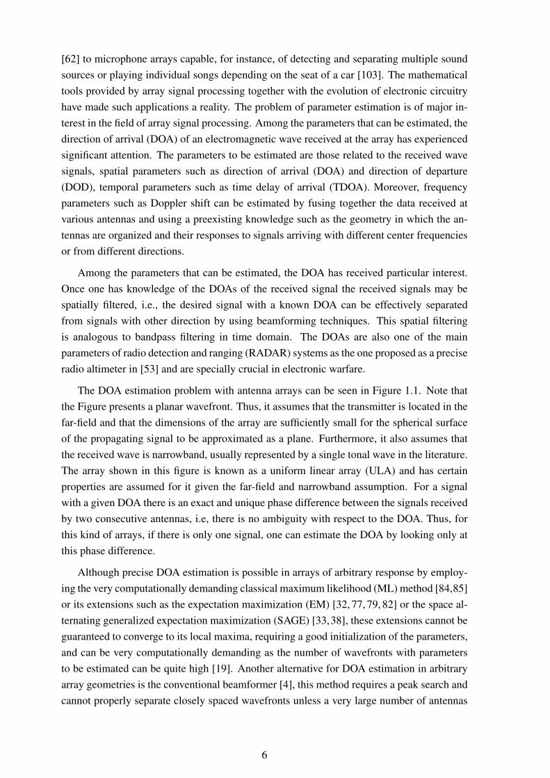
1.1 Signal with DOA θ impinging on a uniform linear array (ULA), whose theantenna space is ∆ ............................................................................ 7
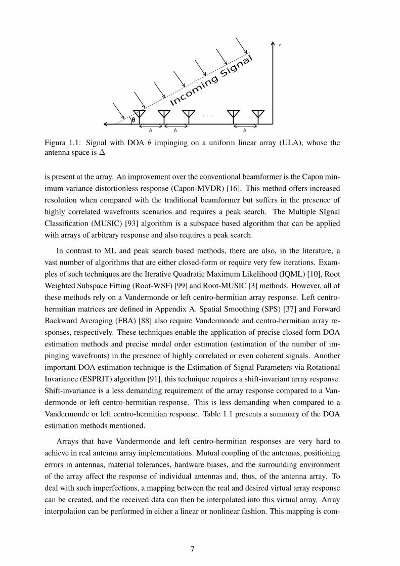
1.2 On the left side there is real data from an antenna array, while on the rightside the data transformed by the transformation matrix B ........................... 8
1.3 Graphical representation of a linear array ................................................ 111.4 Example of SPS subarrays ................................................................... 131.5 Eigenvalue profile: eigenvalue index versus eingenvalue............................. 141.6 P (θ, φ) ............................................................................................ 221.7 Selected sectors and example of sector bounds ......................................... 231.8 Selected sectors and respective bounds for one-dimensional case.................. 251.9 UT of the approximated lc(X;θ,φ) for two sources .................................. 261.10 Example of transformed regions ............................................................ 291.11 Transformation error with respect to combined sector size .......................... 301.12 Example of estimated model order versus number of subarrays .................... 311.13 Tensor B ∈ R2×2×2 ............................................................................. 341.14 Results for a standard deviation of π
20radians ........................................... 41
1.15 Results for a standard deviation of π10
radians ........................................... 411.16 Results for a standard deviation of π
5radians ............................................ 42
1.17 6x1 antenna array: ANSYS HFSS model (left), prototype (right). ................ 431.18 DOA estimation performance with 0.4 λ element separation........................ 441.19 DOA estimation performance with 0.2 λ element separation........................ 451.20 DOA estimation performance for model built with simulated data with 0.4 λ
element separation ............................................................................. 451.21 DOA estimation performance for model built with simulated data with 0.2 λ
element separation ............................................................................. 461.22 TLS-ESPRIT failure rate for 0.2 λ element separation................................ 46
2.1 Examples of peer-to-peer and cluster networks ......................................... 522.2 Example of cooperative MIMO and SISO communications in a wireless sen-
sor network....................................................................................... 522.3 C-MIMO communication steps ............................................................. 532.4 Performance comparison between standard SISO systems and 2× 2 MIMO
systems using ZF, MMSE and ML equalization ........................................ 55
vii

2.5 Examples of single-hop and multi-hop communication............................... 562.6 Performance comparison of equalization methods in the presence of syn-
chronization errors in a 2x2 MIMO system .............................................. 622.7 Performance comparison of equalization methods in the presence of syn-
chronization errors in a 4x4 MIMO system .............................................. 632.8 Performance comparison of equalization methods in the presence of syn-
chronization errors in a 7x7 MIMO system .............................................. 642.9 Performance of ML synchronization,
f =20 MHz, B = 22 MHz................................................................... 652.10 Performance of proposed DFT based synchronization, f =20 MHz, B = 22
MHz ............................................................................................... 662.11 Histogram of synchronization error using the ML method (2.22,2.24) ........... 672.12 Histogram of synchronization error using the DFT method (2.25)................. 672.13 Comparison of individual node energy depletion using C-MIMO or multihop
only ................................................................................................ 762.14 Comparison of individual node energy depletion using multihop only after
2500 seconds .................................................................................... 782.15 Comparison of individual node energy depletion using C-MIMO after 2500
seconds............................................................................................ 782.16 Comparison of individual node energy depletion using multihop only after
4500 seconds .................................................................................... 782.17 Comparison of individual node energy depletion using C-MIMO after 4500
seconds............................................................................................ 782.18 Comparison of individual node energy depletion using multihop only after
5500 seconds .................................................................................... 782.19 Comparison of individual node energy depletion using C-MIMO after 5500
seconds............................................................................................ 782.20 Example of WSN areas with different energetic demands ........................... 792.21 Mean available energy at the center region of the network........................... 792.22 Mean available energy at the edges of the network .................................... 802.23 Standard deviation of available energy at the center region of the network ...... 802.24 Standard deviation of available energy at the edges of the network................ 81
3.1 Scenario description for two vehicles ..................................................... 883.2 Block diagram for the proposed flip-flop method ...................................... 903.3 System model composed of a URA at the base station and an antenna array
at the UAV. ....................................................................................... 943.4 Definitions of pitch α, yaw β and roll γ .................................................. 953.5 Position estimation error vs SNR........................................................... 973.6 Position estimation error vs distance from source ...................................... 983.7 Position estimation error vs number of NLOS components.......................... 98

3.8 Position estimation error vs K-factor ...................................................... 993.9 Position estimation error over the x- and y-axes ........................................ 993.10 Antenna array and an overview of its placement ....................................... 1003.11 Patio where measurements were performed and map of user distribution........ 1003.12 Position estimation error for measured data using the proposed joint estimation1013.13 Position estimation error for measured data using the proposed flip-flop esti-
mation ............................................................................................. 1023.14 Representação gráfica da interpolação de arranjos ..................................... 1073.15 Performance da estimação de direção de chegada com um arranjo com sepa-
ração entre elementos de 0.4 λ .............................................................. 1083.16 Performance da estimação de direção de chegada com um arranjo com sepa-
ração entre elementos de 0.2 λ .............................................................. 1093.17 Comparação da reserva energética dos nós da redes sem MIMO após 2500
segundos .......................................................................................... 1113.18 Comparação da reserva energética dos nós da redes com MIMO após 2500
segundos .......................................................................................... 1113.19 Comparação da reserva energética dos nós da redes sem MIMO após 4500
segundos .......................................................................................... 1113.20 Comparação da reserva energética dos nós da redes com MIMO após 4500
segundos .......................................................................................... 1113.21 Comparação da reserva energética dos nós da redes sem MIMO após 5500
segundos .......................................................................................... 1113.22 Comparação da reserva energética dos nós da redes com MIMO após 5500
segundos .......................................................................................... 1113.23 Erro na estimação de posição utilizando dados reais para a estimação conjunta 1123.24 Erro na estimação de posição utilizando dados reais para a estimação iterativa 112
F.1 GRNN as a parallel neural network ........................................................ 140
G.1 Polarization ellipse ............................................................................. 141

List of Tables
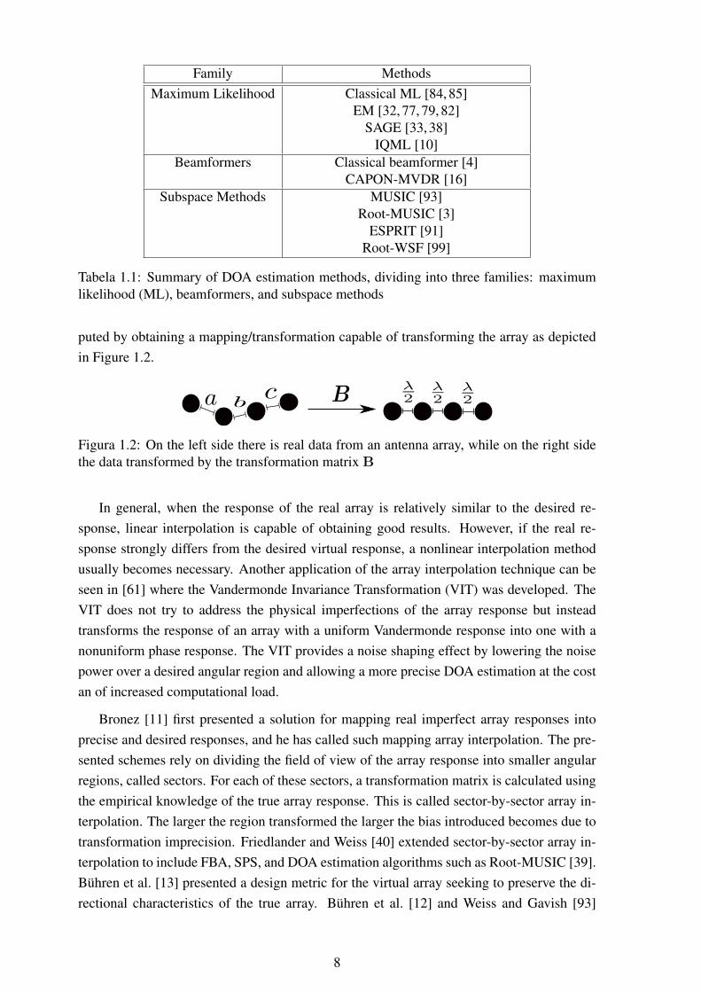
1.1 Summary of DOA estimation methods, dividing into three families: maxi-mum likelihood (ML), beamformers, and subspace methods........................ 8
2.1 Energy consumption for the Mica2 platform ............................................ 572.2 Transmission energy consumption ......................................................... 602.3 Total network energy consumption ........................................................ 752.4 Undeliverable packets ......................................................................... 75
x

Introduction
This work aims to make possible the application of signal processing techniques in sce-narios that were previously unsuitable for it. To this end, the topic of array interpolation isaddressed, allowing imperfect arrays to be used for array processing. Furthermore, in thisdissertation, array signal processing techniques are proposed for wireless sensor networksand vehicular networks.
The following research questions are addressed in this work:
1. How to estimate the directions of arrival of correlated sources that are impinging onan antenna array that does not possess the necessary characteristics (geometry or elec-tromagnetic response) for doing so?
2. Can array processing techniques be used to provide improved lifetime and communi-cation performance in wireless sensor network?
3. Can array processing techniques be used to reliably estimate position of vehicles andpedestrians in vehicular scenarios based on their radio transmissions?
While the overall goal of this thesis is to apply array processing to practical scenar-ios, to allow the reader more freedom each research question is discussed on an individualchapter. Each chapter is presented as self-contained as possible. Therefore, the reader mayread Chapter 1, Chapter 2, Chapter 3 independently. At the beginning of each chapter anoverview, listing the contents of the chapter to allow the reader to skip to sections of interest.Together with the overview, a detailed list of the contributions is presented. Furthermore,each chapter is given its own section providing a brief summary of the discussion containedwithin, presented in Section 1.12, Section 2.8, and Section 3.9, respectively.
The first question is addressed in Chapter 1, where robust array interpolation methods areproposed. By applying array interpolation, data with arbitrary geometries or responses can betransformed into a tractable mathematical model. The problem of interpolation is addressedfrom the ground up, and problems, such as the array discretization, are tackled. Linearand nonlinear interpolation approaches are shown, providing a wide spectrum of alternativesthat can be used according to the desired accuracy and computational complexity of theapplication. By using numerical simulations and measurements, this work shows that theproposed methods outperform the state-of-the-art approaches. Section 1.2 presents a detailed
1

background, and motivation on array interpolation. The six major contributions presented isthis chapter are:
1. A signal adaptive approach for sector detection. Avoiding the pitfalls of having to dealwith multiple sectors or the bias introduced by transforming the entire field of view ofthe array.
2. Two well defined methods for sector discretization aiming to preserve the statisticalintegrity of the transformed regions while minimizing the dimensionality of the data.
3. A linear approach for interpolation that aims to maximize the transformed signal re-gions while minimizing the transformation error, minimizing the parameter estimationbias.
4. A nonlinear extension for the linear approach, allowing the application of the proposedlinear method to arrays with an arbitrary number of dimensions.
5. Two nonlinear array interpolation methods. The nonlinear approaches are suitable fordealing with arrays with highly distorted responses or improper geometries.
6. The performance of the proposed methods is tested using real antenna measurements,validating the proposed methods under real scenarios.
Chapter 2 deals with the second research question. The developed array interpolationtools can be employed to distributed antenna systems, such as wireless sensor networks(WSNs). While interpolated clusters can perform beamforming and detect radio signalsources, a more critical problem in WSNs is the energy efficiency, specially with respectto communication. Another antenna array technique, the multiple-input multiple-output(MIMO) communication technique can be used to achieve improved energy efficiency. How-ever, to this end, it is necessary to achieve a very high degree of synchronization. The prob-lem of synchronization is tackled, and its effects on the performance of MIMO systems areassessed in detail. The energy performance of distributed MIMO systems is analysed, anda threshold for its application is derived. The energetic performance of a network employ-ing cooperative MIMO is shown considerably outperforms state-of-the-art single-hop andmulti-hop methods. A detailed introduction on the topic of cooperative MIMO in WSNs ispresented in Section 2.2. The five major contributions presented is this chapter are:
1. A study on the energy efficiency of C-MIMO with respect to multi and single-hopcommunications, defining a threshold of selection between the multiple communica-tion techniques.
2. An analysis on the impact of synchronization errors in distributed MIMO system withrespect to the symbol period and the size of the communication clusters involved.
2
3. A study on the propagation of synchronization errors inside a WSN, and from thatthe derivation of a closed form expression regarding the resynchronization interval indistributed MIMO systems that takes into account the symbol duration and the clockdrift of the nodes involved.
4. Two methods for synchronization for WSNs with different trade-offs between perfor-mance and computational complexity.
5. An adaptive method for selecting the cluster size of C-MIMO transmissions capableof maximizing energy efficiency and improve the homogeneity of the energy reservesacross the network.
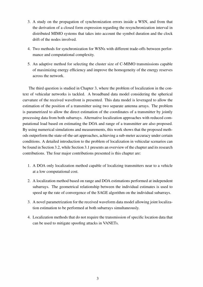
The third question is studied in Chapter 3, where the problem of localization in the con-text of vehicular networks is tackled. A broadband data model considering the sphericalcurvature of the received wavefront is presented. This data model is leveraged to allow theestimation of the position of a transmitter using two separate antenna arrays. The problemis parametrized to allow the direct estimation of the coordinates of a transmitter by jointlyprocessing data from both subarrays. Alternative localization approaches with reduced com-putational load based on estimating the DOA and range of a transmitter are also proposed.By using numerical simulations and measurements, this work shows that the proposed meth-ods outperform the state-of-the-art approaches, achieving a sub-meter accuracy under certainconditions. A detailed introduction to the problem of localization in vehicular scenarios canbe found in Section 3.2, while Section 3.1 presents an overview of the chapter and its researchcontributions. The four major contributions presented is this chapter are:
1. A DOA only localization method capable of localizing transmitters near to a vehicleat a low computational cost.
2. A localization method based on range and DOA estimations performed at independentsubarrays. The geometrical relationship between the individual estimates is used tospeed up the rate of convergence of the SAGE algorithm on the individual subarrays.
3. A novel parametrization for the received waveform data model allowing joint localiza-tion estimation to be performed at both subarrays simultaneously.
4. Localization methods that do not require the transmission of specific location data thatcan be used to mitigate spoofing attacks in VANETs.
3

Chapter 1
Array Interpolation
In this chapter the following research question is addressed:How to estimate the directions of arrival of correlated sources that are impinging on an an-tenna array that does not possess the necessary characteristics (geometry or electromagneticresponse) for doing so?
1.1 Overview and Contribution
The remainder of this section is organized as follows:
• Motivation: The problem of direction of arrival estimation is discussed and a detailedintroduction on the subject of array interpolation presented along with the challengesthis work aims to tackle.
• Data Model: The spatial data model of a signal received at an antenna array is defined.
• Preliminaries: Here important concepts (spatial smoothing, forward backward aver-age, Vandermonde invariant transformation, model order selection, and Estimation ofSignal Parameters via Rotational Invariance Techniques) used throughout the remain-der of this chapter are presented in detail.
• Array Interpolation: The problem of array interpolation is defined and a distinctionbetween linear and nonlinear interpolation is made.
• Classical Interpolation: Here the prior methods available in the literature for arrayinterpolation are briefly detailed.
• Sector Detection and Discretization: A signal adaptive approach that allows sectorsof interest to be detected based on the received signal power is presented. Furthermore,the problem of discretizing these sectors is addressed with two different approachesintroduced, employing the unscented transform (UT) and principal component analysis(PCA) receptively.
4

• Linear Interpolation: This section presents a linear interpolation approach that aimsto minimize the transformation bias while transforming as much as possible of thereceived signal. A calculation of a transform matrix employing the UTs parametersis discussed. The problem of selecting the proper smoothing length for proper signaldecorrelation is discussed.
• Multidimensional Interpolation: Here, a multidimensional extension of the linearapproach is presented. To derive this extension a multidimensional data model is pre-sented and important tensor algebra concepts are detailed.
• Nonlinear Interpolation: This section presents two approaches for performing arrayinterpolation in a nonlinear fashion. A general regression neural network (GRNN) anda multivariate adaptive regression splines (MARS) based approach are detailed.
• Simulation Results: Finally, the performance of the proposed methods is shown bymeans of numerical simulations. A set of such simulations is performed using a realmeasured response from an antenna array in order to validate the proposed methodsusing real data.
The research contributions presented in this chapter are:
1. A signal adaptive approach for sector detection. Avoiding the pitfalls of having to dealwith multiple sectors or the bias introduced by transforming the entire field of view ofthe array.
2. Two well defined methods for sector discretization aiming to preserve the statisticalintegrity of the transformed regions while minimizing the dimensionality of the data.
3. A linear approach for interpolation that aims to maximize the transformed signal re-gions while minimizing the transformation error, minimizing the parameter estimationbias.
4. A nonlinear extension for the linear approach, allowing the application of the proposedlinear method to arrays with an arbitrary number of dimensions.
5. Two nonlinear array interpolation methods. The nonlinear approaches are suitable fordealing with arrays with highly distorted responses or improper geometries.
6. The performance of the proposed methods is tested using real antenna measurements,validating the proposed methods under real scenarios.
1.2 Motivation
Sensor arrays have been applied in various fields of modern electrical engineering [59].From up and coming applications such as massive Multiple Input Multiple Output (MIMO)
5
[62] to microphone arrays capable, for instance, of detecting and separating multiple soundsources or playing individual songs depending on the seat of a car [103]. The mathematicaltools provided by array signal processing together with the evolution of electronic circuitryhave made such applications a reality. The problem of parameter estimation is of major in-terest in the field of array signal processing. Among the parameters that can be estimated, thedirection of arrival (DOA) of an electromagnetic wave received at the array has experiencedsignificant attention. The parameters to be estimated are those related to the received wavesignals, spatial parameters such as direction of arrival (DOA) and direction of departure(DOD), temporal parameters such as time delay of arrival (TDOA). Moreover, frequencyparameters such as Doppler shift can be estimated by fusing together the data received atvarious antennas and using a preexisting knowledge such as the geometry in which the an-tennas are organized and their responses to signals arriving with different center frequenciesor from different directions.
Among the parameters that can be estimated, the DOA has received particular interest.Once one has knowledge of the DOAs of the received signal the received signals may bespatially filtered, i.e., the desired signal with a known DOA can be effectively separatedfrom signals with other direction by using beamforming techniques. This spatial filteringis analogous to bandpass filtering in time domain. The DOAs are also one of the mainparameters of radio detection and ranging (RADAR) systems as the one proposed as a preciseradio altimeter in [53] and are specially crucial in electronic warfare.
The DOA estimation problem with antenna arrays can be seen in Figure 1.1. Note thatthe Figure presents a planar wavefront. Thus, it assumes that the transmitter is located in thefar-field and that the dimensions of the array are sufficiently small for the spherical surfaceof the propagating signal to be approximated as a plane. Furthermore, it also assumes thatthe received wave is narrowband, usually represented by a single tonal wave in the literature.The array shown in this figure is known as a uniform linear array (ULA) and has certainproperties are assumed for it given the far-field and narrowband assumption. For a signalwith a given DOA there is an exact and unique phase difference between the signals receivedby two consecutive antennas, i.e, there is no ambiguity with respect to the DOA. Thus, forthis kind of arrays, if there is only one signal, one can estimate the DOA by looking only atthis phase difference.
Although precise DOA estimation is possible in arrays of arbitrary response by employ-ing the very computationally demanding classical maximum likelihood (ML) method [84,85]or its extensions such as the expectation maximization (EM) [32, 77, 79, 82] or the space al-ternating generalized expectation maximization (SAGE) [33,38], these extensions cannot beguaranteed to converge to its local maxima, requiring a good initialization of the parameters,and can be very computationally demanding as the number of wavefronts with parametersto be estimated can be quite high [19]. Another alternative for DOA estimation in arbitraryarray geometries is the conventional beamformer [4], this method requires a peak search andcannot properly separate closely spaced wavefronts unless a very large number of antennas
6
Y
. . .
Δ Δ Δ
θ
Inco
min
g Sig
nal
Figura 1.1: Signal with DOA θ impinging on a uniform linear array (ULA), whose theantenna space is ∆
is present at the array. An improvement over the conventional beamformer is the Capon min-imum variance distortionless response (Capon-MVDR) [16]. This method offers increasedresolution when compared with the traditional beamformer but suffers in the presence ofhighly correlated wavefronts scenarios and requires a peak search. The Multiple SIgnalClassification (MUSIC) [93] algorithm is a subspace based algorithm that can be appliedwith arrays of arbitrary response and also requires a peak search.
In contrast to ML and peak search based methods, there are also, in the literature, avast number of algorithms that are either closed-form or require very few iterations. Exam-ples of such techniques are the Iterative Quadratic Maximum Likelihood (IQML) [10], RootWeighted Subspace Fitting (Root-WSF) [99] and Root-MUSIC [3] methods. However, all ofthese methods rely on a Vandermonde or left centro-hermitian array response. Left centro-hermitian matrices are defined in Appendix A. Spatial Smoothing (SPS) [37] and ForwardBackward Averaging (FBA) [88] also require Vandermonde and centro-hermitian array re-sponses, respectively. These techniques enable the application of precise closed form DOAestimation methods and precise model order estimation (estimation of the number of im-pinging wavefronts) in the presence of highly correlated or even coherent signals. Anotherimportant DOA estimation technique is the Estimation of Signal Parameters via RotationalInvariance (ESPRIT) algorithm [91], this technique requires a shift-invariant array response.Shift-invariance is a less demanding requirement of the array response compared to a Van-dermonde or left centro-hermitian response. This is less demanding when compared to aVandermonde or left centro-hermitian response. Table 1.1 presents a summary of the DOAestimation methods mentioned.
Arrays that have Vandermonde and left centro-hermitian responses are very hard toachieve in real antenna array implementations. Mutual coupling of the antennas, positioningerrors in antennas, material tolerances, hardware biases, and the surrounding environmentof the array affect the response of individual antennas and, thus, of the antenna array. Todeal with such imperfections, a mapping between the real and desired virtual array responsecan be created, and the received data can then be interpolated into this virtual array. Arrayinterpolation can be performed in either a linear or nonlinear fashion. This mapping is com-
7
Family MethodsMaximum Likelihood Classical ML [84, 85]
EM [32, 77, 79, 82]SAGE [33, 38]
IQML [10]Beamformers Classical beamformer [4]
CAPON-MVDR [16]Subspace Methods MUSIC [93]
Root-MUSIC [3]ESPRIT [91]
Root-WSF [99]
Tabela 1.1: Summary of DOA estimation methods, dividing into three families: maximumlikelihood (ML), beamformers, and subspace methods
puted by obtaining a mapping/transformation capable of transforming the array as depictedin Figure 1.2.
Figura 1.2: On the left side there is real data from an antenna array, while on the right sidethe data transformed by the transformation matrix B
In general, when the response of the real array is relatively similar to the desired re-sponse, linear interpolation is capable of obtaining good results. However, if the real re-sponse strongly differs from the desired virtual response, a nonlinear interpolation methodusually becomes necessary. Another application of the array interpolation technique can beseen in [61] where the Vandermonde Invariance Transformation (VIT) was developed. TheVIT does not try to address the physical imperfections of the array response but insteadtransforms the response of an array with a uniform Vandermonde response into one with anonuniform phase response. The VIT provides a noise shaping effect by lowering the noisepower over a desired angular region and allowing a more precise DOA estimation at the costan of increased computational load.
Bronez [11] first presented a solution for mapping real imperfect array responses intoprecise and desired responses, and he has called such mapping array interpolation. The pre-sented schemes rely on dividing the field of view of the array response into smaller angularregions, called sectors. For each of these sectors, a transformation matrix is calculated usingthe empirical knowledge of the true array response. This is called sector-by-sector array in-terpolation. The larger the region transformed the larger the bias introduced becomes due totransformation imprecision. Friedlander and Weiss [40] extended sector-by-sector array in-terpolation to include FBA, SPS, and DOA estimation algorithms such as Root-MUSIC [39].Bühren et al. [13] presented a design metric for the virtual array seeking to preserve the di-rectional characteristics of the true array. Bühren et al. [12] and Weiss and Gavish [93]
8
presented methods for array interpolation that allow the application of ESPRIT for DOAestimation. All of these interpolation methods are performed on by sector-by-sector basis,dividing the entire field of view of the array and performing multiple DOA estimations, onefor each sector.
When performing array interpolation for a sector there is no guarantee with respect towhat happens with signals received from outside the angular region for which the transforma-tion matrix was derived (out-of-sector signals). If the out-of-sector signal is correlated withany possible in-sector signal, a large bias in the DOA estimation is introduced. Pesaventoet al. [87] proposed a method for filtering out of sector signals using cone programming. Asimilar approach was used by Lau et al. [63, 64] where correlated out-of-sector signals wereaddressed by filtering out the out-of-sector signals.
More recently, array interpolation has been applied to more specific scenarios. Liu etat. [68] extended the concept of linear array interpolation to coprime arrays allowing forbetter identifiability of received signals. Hosseini and Sebt [52] applied the concept of lineararray interpolation to sparse arrays by selecting virtual arrays as small as possible whileretaining the aperture of the original sparse array.
This work proposes an adaptive single sector selection method aiming to circumventthe problem of out-of-sector signals by interpolating all regions of the array where poweris received using a single transformation. This work presents an alternative for applyingESPRIT with FBA and SPS, relying on a signal adaptive sector construction and discretiza-tion and extended the method to the multidimensional case. The proposed method preventsout-of-sector problems by building a single sector using a signal adaptive approach whilealso bounding the transformation error. This, however, can lead to large sectors and, in thecase of a small number of antennas, this will lead to larger transformation errors and DOAestimation biases. To deal with these limitations, the work at hand also presents a novel pre-processing step used for sector discretization based on PCA and derives a novel concept fromthe UT [73]. Furthermore, this work extends the concepts of linear interpolation and sectorselection to the muldimensional case, allowing the application of the proposed methods isarrays and data models with an arbitrary number of dimensions.
This work proposes a novel nonlinear interpolation approach using MARS. The proposedapproach is capable of interpolating arrays with a limited number of antennas and very dis-torted responses while keeping the DOA estimation bias low, heavily outperforming arraylinear interpolation methods. This performance improvement comes at the cost of increasedcomputational cost. This work extends the MARS with advanced sector discretization meth-ods that lead to a better performance and lower complexity. Furthermore, a more detailedmathematical description of the MARS method is presented. Expanding on the topic of non-linear interpolation, the work at hand additionally presents an novel interpolation approachbased on GRNNs. The proposed method is capable of achieving a performance similar tothat of MARS in certain SNR regimes at a lower computational cost compared to the MARSbased method.
9
In summary, this work extends the concepts of array interpolation presented in previousresearch to explore the concepts of statistical significant sector discretization and nonlin-ear interpolation. Previous research focused on concepts for sector-by-sector processing,whereas this work aims to use a single unified sector discretized in a statistically significantmanner. Moreover, this work develops novel nonlinear methods for array interpolation andpresents a method suitable for real-time implementations capable of providing better perfor-mance than linear interpolation methods previously derived in the literature.
The results of the proposed discretization and interpolation methods are assessed via aset of studies considering measured responses obtained from a real physical system. Theresults show that all the proposed methods significantly improve DOA estimation consider-ing a physical system and its inherent imperfections. Furthermore, this work analyses theperformance of the proposed interpolation methods when measurements of the true array re-sponse are not available and only simulated responses for building the interpolation modelsare available.
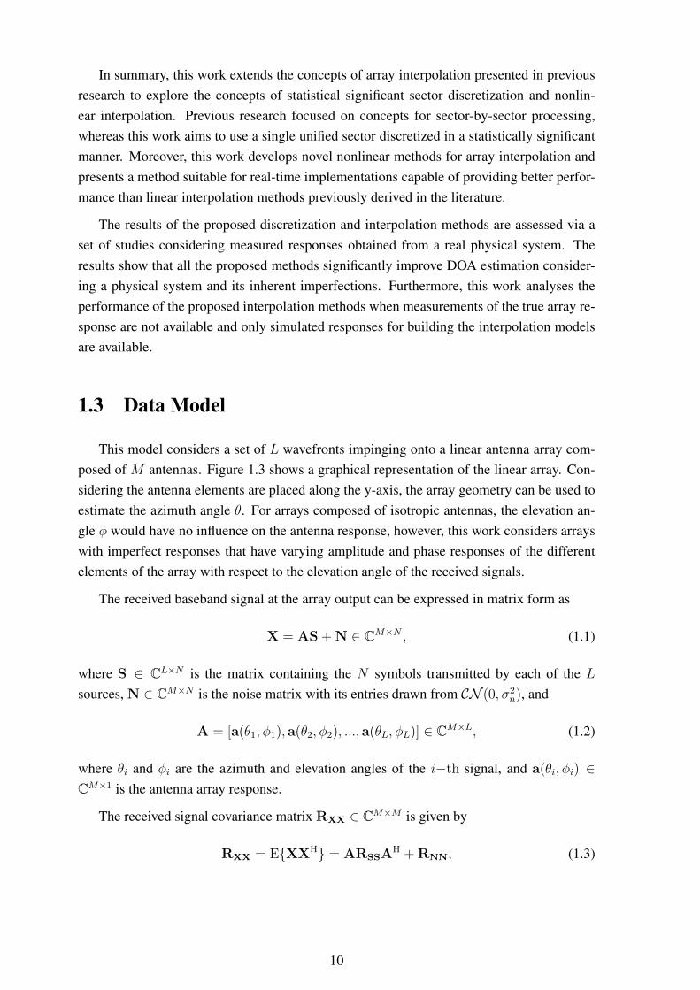
1.3 Data Model
This model considers a set of L wavefronts impinging onto a linear antenna array com-posed of M antennas. Figure 1.3 shows a graphical representation of the linear array. Con-sidering the antenna elements are placed along the y-axis, the array geometry can be used toestimate the azimuth angle θ. For arrays composed of isotropic antennas, the elevation an-gle φ would have no influence on the antenna response, however, this work considers arrayswith imperfect responses that have varying amplitude and phase responses of the differentelements of the array with respect to the elevation angle of the received signals.
The received baseband signal at the array output can be expressed in matrix form as
X = AS + N ∈ CM×N , (1.1)
where S ∈ CL×N is the matrix containing the N symbols transmitted by each of the Lsources, N ∈ CM×N is the noise matrix with its entries drawn from CN (0, σ2
n), and
A = [a(θ1, φ1), a(θ2, φ2), ..., a(θL, φL)] ∈ CM×L, (1.2)
where θi and φi are the azimuth and elevation angles of the i−th signal, and a(θi, φi) ∈CM×1 is the antenna array response.
The received signal covariance matrix RXX ∈ CM×M is given by
RXX = E{XXH} = ARSSAH + RNN, (1.3)
10
φ
θ
x
y
z
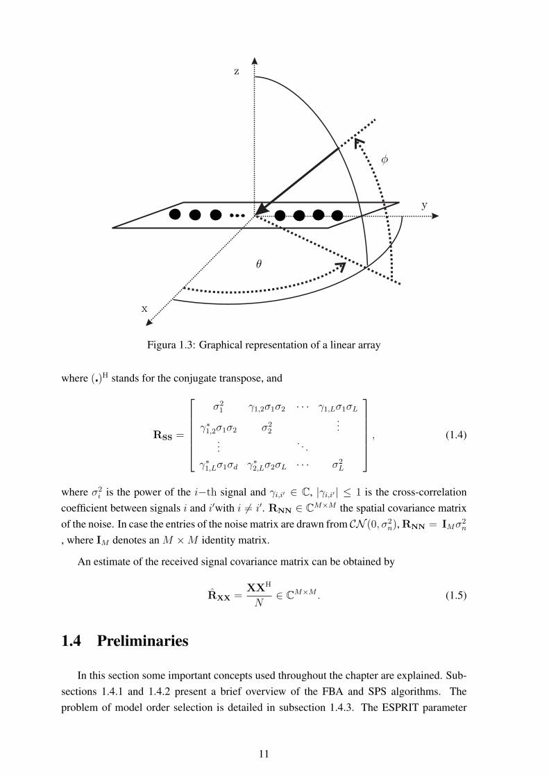
Figura 1.3: Graphical representation of a linear array
where (�)H stands for the conjugate transpose, and
RSS =
σ2
1 γ1,2σ1σ2 · · · γ1,Lσ1σL
γ∗1,2σ1σ2 σ22
......
. . .
γ∗1,Lσ1σd γ∗2,Lσ2σL · · · σ2L
, (1.4)
where σ2i is the power of the i−th signal and γi,i′ ∈ C, |γi,i′| ≤ 1 is the cross-correlation
coefficient between signals i and i′with i 6= i′. RNN ∈ CM×M the spatial covariance matrixof the noise. In case the entries of the noise matrix are drawn from CN (0, σ2
n), RNN = IMσ2n
, where IM denotes an M ×M identity matrix.
An estimate of the received signal covariance matrix can be obtained by
RXX =XXH
N∈ CM×M . (1.5)
1.4 Preliminaries
In this section some important concepts used throughout the chapter are explained. Sub-sections 1.4.1 and 1.4.2 present a brief overview of the FBA and SPS algorithms. Theproblem of model order selection is detailed in subsection 1.4.3. The ESPRIT parameter
11
estimation algorithm is shown in subsection 1.4.4. Finally, subsection 1.4.5 explains thevandermonde invariance transformation (VIT).
1.4.1 Forward Backward Averaging (FBA)
In the case where only two highly correlated or coherent sources are present the FBA [88]is capable of decorrelating the signals and allowing the application of subspace based meth-ods. For an uniform linear array (ULA) or uniform rectangular array (URA) the steeringvectors remain invariant, up to scaling, if their elements are reversed and complex conju-gated. Let Q ∈ ZM×M by an exchange matrix with ones on its anti-diagonal and zeroselsewhere as defined in (4). Then, for a M element ULA it holds that
QA* = A. (1.6)
The forward backward averaged covariance matrix can be obtained as
RXXFBA=
1
2(RXX + QR∗XXQ). (1.7)
By looking into the structure of the covariance matrix shown in (1.3), (1.7) can be rewrittenas
RXXFBA= A
1
2(RSS + R∗SS)AH +
1
2(RNN + QRNN
∗Q). (1.8)
The results is that the matrix RSS + R∗SS = 2<(RSS) is composed of purely real numbers,that is, if the correlation coefficient between the signals is given by a purely imaginary num-ber then the FBA offers maximum decorrelation, if, however, the correlation coefficient isgiven only by a real number, then the FBA offers no improvement regarding signal decorre-lation. FBA can also be used with the sole purpose of improving the variance of the estimatesby virtually doubling the number of available samples without resulting in noise correlation.
1.4.2 Spatial Smoothing (SPS)
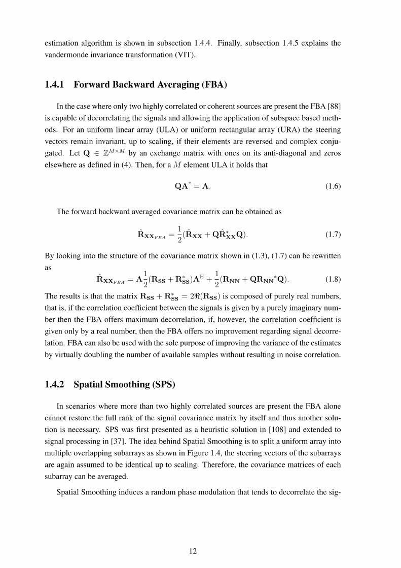
In scenarios where more than two highly correlated sources are present the FBA alonecannot restore the full rank of the signal covariance matrix by itself and thus another solu-tion is necessary. SPS was first presented as a heuristic solution in [108] and extended tosignal processing in [37]. The idea behind Spatial Smoothing is to split a uniform array intomultiple overlapping subarrays as shown in Figure 1.4, the steering vectors of the subarraysare again assumed to be identical up to scaling. Therefore, the covariance matrices of eachsubarray can be averaged.
Spatial Smoothing induces a random phase modulation that tends to decorrelate the sig-
12
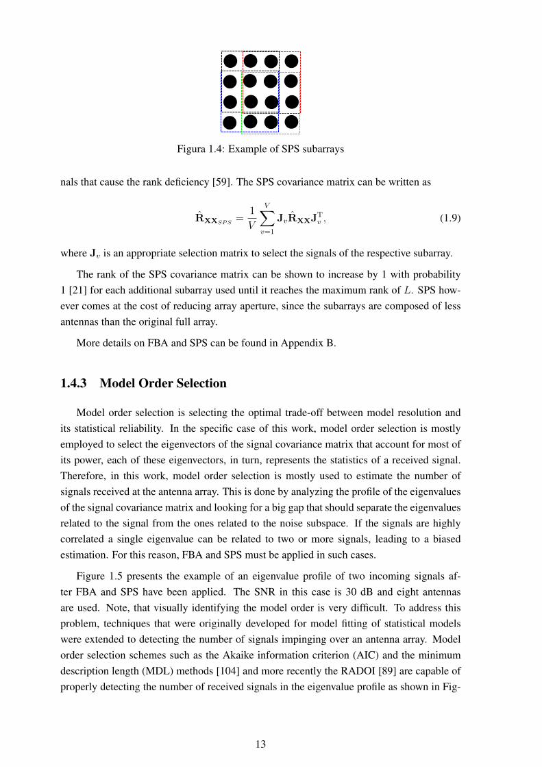
Figura 1.4: Example of SPS subarrays
nals that cause the rank deficiency [59]. The SPS covariance matrix can be written as
RXXSPS=
1
V
V∑v=1
JvRXXJTv , (1.9)
where Jv is an appropriate selection matrix to select the signals of the respective subarray.
The rank of the SPS covariance matrix can be shown to increase by 1 with probability1 [21] for each additional subarray used until it reaches the maximum rank of L. SPS how-ever comes at the cost of reducing array aperture, since the subarrays are composed of lessantennas than the original full array.
More details on FBA and SPS can be found in Appendix B.
1.4.3 Model Order Selection
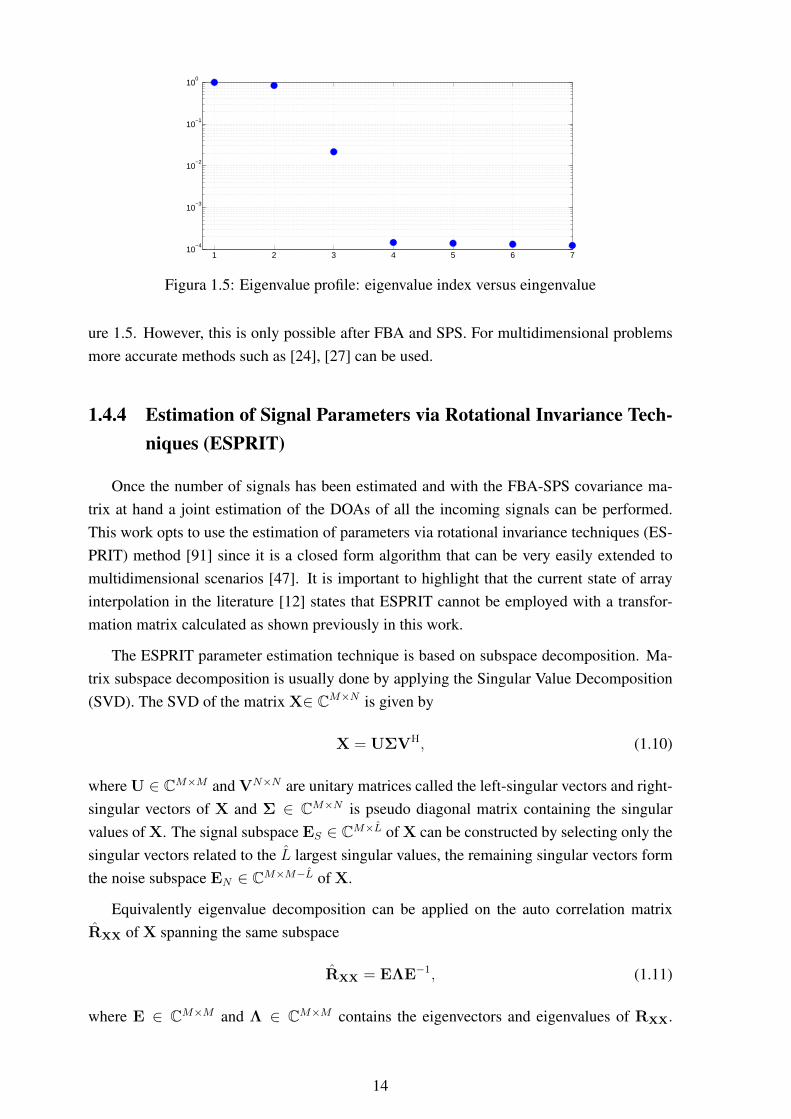
Model order selection is selecting the optimal trade-off between model resolution andits statistical reliability. In the specific case of this work, model order selection is mostlyemployed to select the eigenvectors of the signal covariance matrix that account for most ofits power, each of these eigenvectors, in turn, represents the statistics of a received signal.Therefore, in this work, model order selection is mostly used to estimate the number ofsignals received at the antenna array. This is done by analyzing the profile of the eigenvaluesof the signal covariance matrix and looking for a big gap that should separate the eigenvaluesrelated to the signal from the ones related to the noise subspace. If the signals are highlycorrelated a single eigenvalue can be related to two or more signals, leading to a biasedestimation. For this reason, FBA and SPS must be applied in such cases.
Figure 1.5 presents the example of an eigenvalue profile of two incoming signals af-ter FBA and SPS have been applied. The SNR in this case is 30 dB and eight antennasare used. Note, that visually identifying the model order is very difficult. To address thisproblem, techniques that were originally developed for model fitting of statistical modelswere extended to detecting the number of signals impinging over an antenna array. Modelorder selection schemes such as the Akaike information criterion (AIC) and the minimumdescription length (MDL) methods [104] and more recently the RADOI [89] are capable ofproperly detecting the number of received signals in the eigenvalue profile as shown in Fig-
13
1 2 3 4 5 6 710
−4
10−3
10−2
10−1
100
Figura 1.5: Eigenvalue profile: eigenvalue index versus eingenvalue
ure 1.5. However, this is only possible after FBA and SPS. For multidimensional problemsmore accurate methods such as [24], [27] can be used.
1.4.4 Estimation of Signal Parameters via Rotational Invariance Tech-niques (ESPRIT)
Once the number of signals has been estimated and with the FBA-SPS covariance ma-trix at hand a joint estimation of the DOAs of all the incoming signals can be performed.This work opts to use the estimation of parameters via rotational invariance techniques (ES-PRIT) method [91] since it is a closed form algorithm that can be very easily extended tomultidimensional scenarios [47]. It is important to highlight that the current state of arrayinterpolation in the literature [12] states that ESPRIT cannot be employed with a transfor-mation matrix calculated as shown previously in this work.
The ESPRIT parameter estimation technique is based on subspace decomposition. Ma-trix subspace decomposition is usually done by applying the Singular Value Decomposition(SVD). The SVD of the matrix X∈ CM×N is given by
X = UΣVH, (1.10)
where U ∈ CM×M and VN×N are unitary matrices called the left-singular vectors and right-singular vectors of X and Σ ∈ CM×N is pseudo diagonal matrix containing the singularvalues of X. The signal subspace ES ∈ CM×L of X can be constructed by selecting only thesingular vectors related to the L largest singular values, the remaining singular vectors formthe noise subspace EN ∈ CM×M−L of X.
Equivalently eigenvalue decomposition can be applied on the auto correlation matrixRXX of X spanning the same subspace
RXX = EΛE−1, (1.11)
where E ∈ CM×M and Λ ∈ CM×M contains the eigenvectors and eigenvalues of RXX.
14
The eigenvectors related to the L largest eigenvalues span the same signal subspace ES ofthe single value decomposition. The same holds for the noise subspace of the EVD and leftsingular vectors of the SVD, EN .
This classic eigendecomposition is suitable when the noise received at the antenna arrayis spatially white, since, in the case at hand, a transformation is applied to the data, even ifthe received noise was originally white it turns in colored noise. To deal with colored noisethe generalized eigenvalue decomposition (GEVD) can be used to take the noise correlationinto account, the GEVD of the matrix pair RXX, RNN is given by
RXXΓ = RNNΓΛ, (1.12)
where E ∈ CM×M is a matrix containing the generalized eigenvectors and Λ ∈ RM×M is amatrix containing the generalized eigenvalues in its diagonal. Notice that this decompositionis the same as the EVD (1.11) for RNN = I. The subspace ΓS ∈ CM×L is formed selectingthe generalized eigenvectors related to the L largest generalized eigenvalues. This subspace,however, does not span the same column subspace as the original steering matrix, and needsto be reprojected onto the original manifold subspace or dewhitened. This can be done by
Γs = RNNΓs. (1.13)
With this subspace estimate at hand the Total Least Squares (TLS) ESPRIT [91] is applied.Two subsets of the signal subspace that are related trough the shift invariance property needto be selected.
Let Γ1 and Γ2 represent the subspace subsets selected as previously mentioned. A matrixΓ1,2 is constructed as
Γ1,2 =
[ΓH
1
ΓH2
][Γ1Γ2] . (1.14)
Performing an eigendecomposition of Γ1,2 and ordering its eigenvalues in the decreasingorder and its eigenvectors accordingly the eigenvector matrix V can be divided into blocksas
V =
[V1,1 V1,2
V2,1 V2,2
]. (1.15)
Finally, the parameters can be obtained by finding the eigenvalues of
Φ = eig(−V1,2
V2,2
). (1.16)
The parameters in Φ can represent a phase delay respective to a DOA if DOAs are beingestimated, or can represent the ratio of the strength at which a signal appears in the differentpolarizations.
For multidimensional arrays another option is to employ methods based on the parallel
15
factor analysis (PARAFAC) decomposition such as [29], [28] instead of the ESPRIT.
1.4.5 Vandermonde Invariance Transformation (VIT)
Finally, once the first set of estimates has been obtained the VIT can be applied, thistransformation aims to shape the noise away from the regions where the signal is arrivingin order to obtain improved estimates [61] . The VIT is an array interpolation approachthat transforms a vandermonde system with a response linear with respect to the angle ofarrival into an also vandermonde system with a highly nonlinear response with respect to theangle of arrival. The VIT promotes a nonlinear transformation with respect to the selectedspatial frequency µ(θ). Let u = [1, ejµ(θ), . . . , ejµ(θ)(M−1)], the VIT performs the followingtransformation
u(V IT ) = T(θ)u = (ejµ(θ) − r
1− r )
1
ejν(θ)
...
ejν(θ)(M−1)
, (1.17)
r and ν are design parameters that can be chosen considering a compromise between thelevel of noise suppression desired around µ and the linearity of the output.
The VIT can be used to apply a phase attenuation to the dataset, which in turn shapesthe noise, reducing the power of the noise in the region near µ(θ) and increasing it over itsvicinity. Thus, the VIT needs to be applied angle wise, i.e, a set of initial estimates of theangles θ is used to calculate a VIT centered over the given angles, and a second estimateis performed. This second estimation yields and offset θoffset with respect to the original θ,giving the final estimation θVIT = θ + θoffset. Due to the mentioned noise shaping, this finalestimation offers increased precision, but comes at the cost of transforming the dataset andapplying the chosen DOA estimation method L times.
The VIT can be interpreted as a zoom, similar to an optical zoom, with the first estimatesa zoom can be used on the regions of the manifold where signal has been estimated to arrive.The region can be inspected with the zoom effect to detect any imprecisions from the firstestimate. The increased performance comes at the cost of L extra DOA estimations.
1.5 Array Interpolation
Arrays can be interpolated by means of a one-to-one mapping given by
f : AS → AS , (1.18)
where S is a sector. It is worth noting that even if an array has the required geometry for theusage of a certain array processing technique, its response may not adhere to an underlying
16

assumed mathematical model. Therefore, in such cases, geometrically well behaved arraysmay need to be interpolated to allow the application of the desired technique.
Definition 1. A sector S is a finite and countable set of 2-tuples (pairs) of angles (θ, φ)
containing all the combinations of azimuth and elevation angles representing a region of thefield of view of the array. The sector S defines the column space of AS and AS .
AS ∈ CM×|S| is the array response matrix formed out of the array response vectorsa(θ, φ) ∈ CM×1 of the angles given by the elements of S. AS contains the true arrayresponse of the physical system, which may not possess important properties such as beingleft centro-hermitian or Vandermonde. AS ∈ CM ′×|S| is the interpolated version of AS withcolumns a(θ, φ) ∈ CM ′×1 being the array response of the so-called virtual or desired array,having all the properties necessary for posterior processing. |S| is the cardinality of the setS, i.e. the number of elements in the set.
Definition 2. The mapping f is said to be array size preserving if M = M ′.
Definition 3. The mapping f is said to be geometry preserving if it is size preserving and ifthe underlying array geometry for the true and virtual array is equivalent.
This work limits itself to mappings of linear planar arrays that are size and geometrypreserving, as given in Definitions 2 and 3, respectively.
Linear array interpolation is usually done using a least squares approach. The problem isset up as finding a transformation matrix B that is given by
BAS = AS . (1.19)
The snapshot matrix X can be transformed by multiplying it from the left-hand side withthe transform matrix B, which is equivalent to applying a linear model for each of the out-puts of the virtual antenna array. Therefore, in linear array interpolation f is given by thetransformation matrix B.
This model is usually not capable of transforming the response perfectly across the entirefield of view except for the case where a large number of antenna elements is present or a verysmall sector is used. Large transformation errors often result in a large bias on the final DOAestimation, thus, usually, the response region is divided into a set of regions called sectors,and a different transform matrix is set up for each sector (sector-by-sector processing).
Nonlinear interpolation is an alternative to the linear approach capable of providing betteraccuracy under more challenging scenarios at the cost of increased complexity. In nonlinearinterpolation, the mapping f is given by a nonlinear function, such that
f(v + βq) 6= f(v) + βf(q) (1.20)
for some v, q and β.
17
1.6 Classical Interpolation
The SPS and FBA methods shown for decorrelating signals are limited to arrays beingVandermode and/or left centro-hermitian. As mentioned previously such geometries arehard to achieve in real implementations due to problems such as space limitation or the nonlinearity of the antenna lobes with respect to the DOA of received waves. Also, importantsubspace DOA estimation methods such as the Root-MUSIC [3] rely on the ULA geometryand although the ESPRIT [91] requires only the shift invariance property, in the literaturemost authors apply ESPRIT in either a ULA or URA. Thus, to allow the application ofsuch methods is generic arrays some sort of data transformation needs to be used first. Thistype of transformation of known in the literature are array interpolation or array mapping.All the current approaches in the literature use this sector-by-sector processing, the worksin [39], [87] and [13] differ only by the way the matrix A is set up. The linear approach toarray interpolation shown in (1.19) is equivalent to applying a linear model for each of theoutputs of the virtual antenna array. This linear model can be given
[y]m = [B]1,m [y]m + [B]2,m [y]m + . . .+ [B]M,m [y]m , (1.21)
where [·]i,j is the element of a matrix indexed by i and j, and m ∈ {1, . . .M}. In classicalarray interpolation, since the receiver has no prior information about the DOA of the receivedsignals A and A are constructed by dividing the field of view of the array into K continuousregions, called sectors, with upper bound uk and lower bound lk. This is the sector-by-sectorapproach. The region [lk, uk] is then discretized according to
Sk = [lk, lk + ∆, ..., uk −∆, uk], (1.22)
where ∆ is the angular resolution of the transformation. These angles are used to generatethe respective set of steering vectors and construct A and A according to
ASk = [a(lk), a(lk + ∆), ..., a(uk −∆), a(uk)] ∈ CM×uk−lk∆ ,
ASk = [a(lk), a(lk + ∆), ..., a(uk −∆), a(uk)] ∈ CM×uk−lk∆ ,
where M is the number of antennas, including their different polarizations, present at thearray. The transformation is usually not perfect since the transformation matrix B does nothave enough degrees of freedom to transform the entire discrete sector. B is obtained as thebest fit between the transformed response BASk and the desired response ASk , this is doneby applying a least squares fit to the overdetermined systems yielding
B = ASkA†Sk ∈ CM×M , (1.23)
where (·)† is the pseudo inverse of the matrix. To access the precision of the transformationthe Frobenius norm of the errors matrix BASk − ASk is compared with the Frobenius norm
18
of the desired response steering matrix ASk . The error of the transform is defined as
ε(Sk) =
∥∥ASk −BASk∥∥
F∥∥ASk∥∥F
∈ R+. (1.24)
Large transformation errors will results in a large bias in the final DOA estimates. The trans-formation error can, however, be kept as low as desired by making the sectors Sk smaller. Itis worth noting that for the sector-by-sector approach the transformation matrices can be cal-culated off-line, since they do not rely on the received data, and just reused when necessary.
With B at hand the data can be transformed by
X = BX. (1.25)
The transformed covariance is then equivalent to
RXX =BX(BX)H
N=
BXXHBH
N= BRXXBH. (1.26)
From (1.26) it is possible to note that the transformation matrix can instead be applied di-rectly to the covariance matrix. Plugging (1.4) into (1.26) results in
RXX = BARSSAHBH + BRNNBH (1.27)
= ARSSAH + BRNNBH.
Thus, although the transformation transforms A into A as desired it changes the character-istics of RNN. If the noise was previously white it becomes colored or, if the noise wasalready colored, it changes its color. Since most of the methods in the literature assume thatRNN = σ2
nI, i.e, white noise, the next step used in classical interpolation is a noise whiteningstep to restore the diagonal characteristic of RNN
RXX = R− 1
2NNRXXR
−H2
NN, (1.28)
where RNN = BRNNBH. Different methods for array interpolation have been speciallydeveloped in order to apply the ESPRIT algorithm [12, 106]. In these methods a differenttransformation matrix is calculated for each of the shift invariant subarrays used in ESPRIT,in this way the noise between each subarray is not correlated and ESPRIT can be directlyused, these methods, however, do not allow the application of FBA-SPS and thus are inca-pable of being used in the presence of highly correlated signals.
The current state-of-the-art for applying array interpolation in highly correlated signalsis presented in [63, 64]. Normally, if the signals that fall out-of-sector are not correlatedwith the in sector signals the influence of the out-of-sector signals in the processing posteriorto the transformation is not high. On the other hand, if a signal located out-of-sector iscorrelated with an in sector signal, the posterior estimations can be gravely affected. These
19

works try to keep the out-of-sector response under control by taking into account the responseover the entire array manifold. The problem can be formulated as a weighted least squaresproblem [64]
minT
π∫−π
π∫−π
w(θ, φ) ‖Ta(θ, φ)− v(θ, φ)a(θ, φ)‖2 dθ dφ, (1.29)
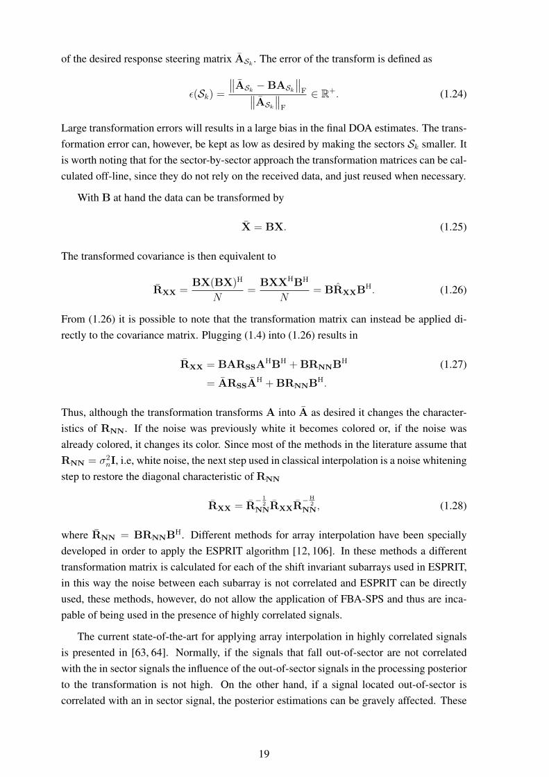
wherew(θ, φ) is an arbitrary weighting function and v(θ, φ) defines the DOA dependent gainthat shapes the array response, it should control the response of the array for out-of-sectorsignals while leaving the response unaltered for signals within the sector. An optimal solutionwould be to set v(θ, φ) as a rectangular function, setting its gain to zero to any DOA outsideof the sector and to 1 for the entire sector. This, however, would result in extremely largetransformation errors, specially due to the discontinuities found in the edges of the sector.Another alternative is to shape v(θ, φ) as a root raised cosine function in θ and φ, allowingthe gain to roll off along the edges of the sector. By defining the sectors ∆θ = [−θ0, θ0] and∆φ = [−φ0, φ0] the gain is given by (1.30).
This approach is capable of dealing with closely spaced and highly correlated out-of-sector signals since it addresses the out-of-sector response. However, since this approachtransforms the entire field of view for each of the sectors used it introduces a large transfor-mation bias in the final estimates.
1.7 Sector Selection and Discretization
Whatever array interpolation method is used, linear or nonlinear, the array response canonly be interpolated after sector detection/selection and sector discretization. The followingsection presents a discussion on detection and selection of sectors of the field of view of theantenna array and how to discretize the detected sectors.
Traditionally, the field of view of the array is divided into sectors that are small enough tokeep the interpolation bias bounded. These sectors can be made larger or smaller dependingon the accuracy desired for the interpolation. After the field of view is divided the sectorsare discretized uniformly using a fine grid and sector-by-sector interpolation is performed.
To avoid performing sector-by-sector interpolation this work uses a single combined sec-tor containing all regions of the field of view of the array where significant power is received.Considering that the response of the true array needs to be known to construct a transforma-tion of the interpolation of the received signal, this response can be used to detect angularregions where significant power is received in order to detect sectors adaptively. To this end,the conventional beamformer [4] can be applied to provide an estimate of angular regions
20
v(θ, φ) =
1, |θ| ≤ θ0 and |φ| ≤ φ0
12
+ 14cos(π(|θ|−θ0)
2θ0−π ) + 14cos(π(|φ|−φ0)
2φ0−π ), θ0 < |θ| ≤ (π − θ0) or φ0 < |φ| ≤ (π − φ0)
0, (π − θ0) < |θ| ≤ π or (π − φ0) < |φ| ≤ π
(1.30)
21
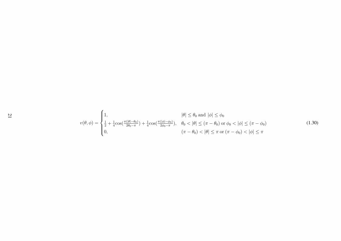
where significant power is received. The beamformer yields the normalized power response
P (θ, φ) =aH(θ, φ) RXX a(θ, φ)
aH(θ, φ) a(θ, φ)∈ R. (1.30)
Since the beamformer is only a delay and sum approach it is not affected by signal correlationand can provide low resolution estimates even in completely correlated signal environments.Although one could argue for using weighted beamformers such as the CAPON-MVDR [16]since this method offers increased resolution when compared the traditional beamformer itsuffers in the presence of highly correlated wavefronts and requires a matrix inversion, lead-ing to a higher computational load. Therefore, this work employs the conventional beam-former in this first step due to its robustness and simplicity.
Figure 1.6 shows an example of the real data output of (1.30) for a signal received at thesix element linear physical antenna array shown in Figure 1.17 with θ = 0◦, φ = 20◦, SNR= 30 dB, and N = 10.
-90 -70 -50 -30 -10 10 30 50 70 90-90
-70
-50
-30
-10
10
30
50
70
90
0.2
0.4
0.6
0.8
1
φ
P(θ,φ
)
θ
Figura 1.6: P (θ, φ)
In physical systems, the result of (1.30) is discrete in θ and φ, and can be written as
P [z, v] = P (−90◦ + (z ·∆θ),−90◦ + (v ·∆φ)) = P (θ, φ), (1.31)
with z ∈ N0, v ∈ N0 , θ ∈ D∆θ, and φ ∈ D∆φ
where
D∆θ= {−90◦,−90◦ + ∆θ, ..., 90◦ −∆θ, 90◦}, (1.32)
D∆φ= {−90◦,−90◦ + ∆φ, ..., 90◦ −∆φ, 90◦}. (1.33)
Here, ∆θ ∈ R+ and ∆φ ∈ R+ are the resolution of the azimuth and elevation angles of thepower response (1.30), respectively.
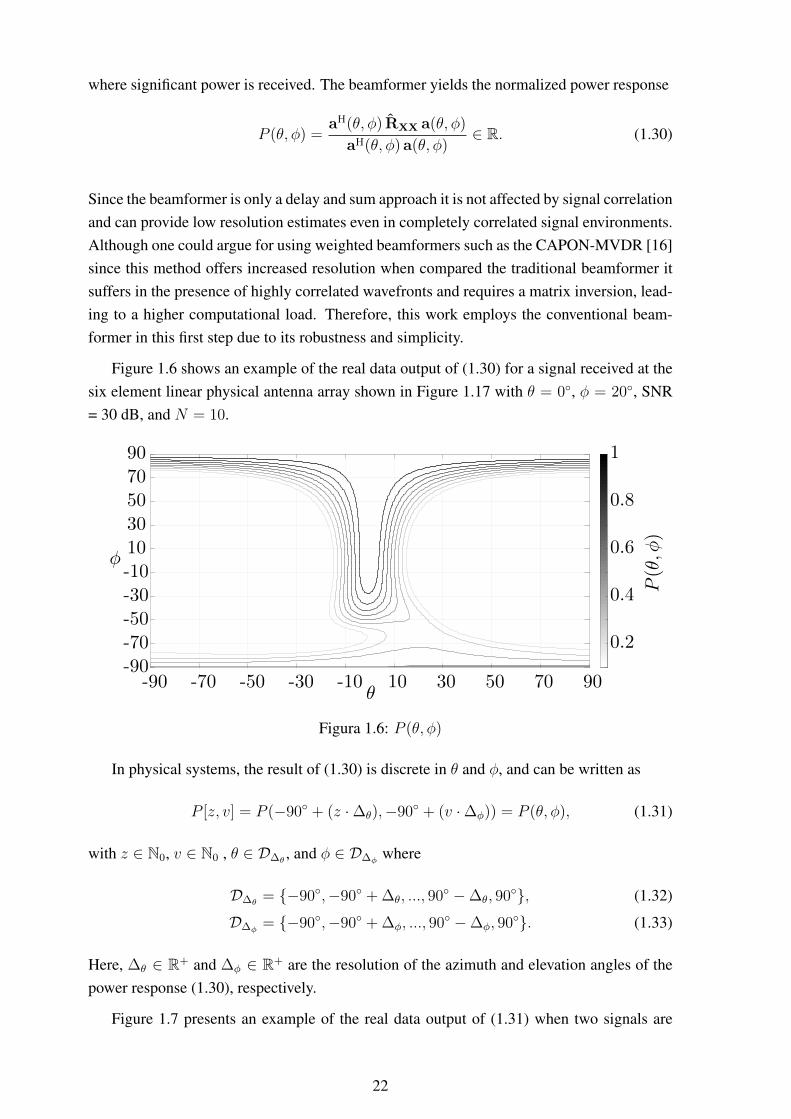
Figure 1.7 presents an example of the real data output of (1.31) when two signals are
22
transmitted from (−5◦,0◦) and (30◦,−10◦), with SNR = 30 dB, and N = 10 at the physicalarray shown in Figure 1.17. This normalized power response is scanned for sectors Sk , andfor each sector, the respective lower bounds θlk ∈ D∆θ
and φlk ∈ D∆φ, as well as the upper
bounds θuk ∈ D∆θand φuk ∈ D∆φ
are defined as shown in Figure 1.7. A threshold ασ2n, with
α ∈ R+, defines a sector Sk considering the criterion P (θ, φ) ≥ ασ2n and k = 1, . . . , K . A
sector can be defined as
Sk = Θk × Φk = {(θ, φ)| θ ∈ Θk ∧ φ ∈ Φk}, (1.34)
where
Θk = {θ| θlk ≤ θ ≤ θuk} ⊆ D∆θ, (1.35)
Φk = {φ|φlk ≤ φ ≤ φuk} ⊆ D∆φ, (1.36)
and∀Kk, k′ = 1
k 6= k′
Sk ∩ Sk′ = ∅. (1.37)
A combined sector can be defined as
S = S1 ∪ · · · ∪ Sk ∪ · · · ∪ SK ⊆ D∆θ×D∆φ
. (1.38)
-90 -70 -50 -30 -10 10 30 50 70 90-90
-70
-50
-30
-10
10
30
50
70
90
0.2
0.4
0.6
0.8
1
P(θ,φ
)
θ
φ
θlk θuk
φlk
φuk
Figura 1.7: Selected sectors and example of sector bounds
Most array signal processing techniques assume the presence of isotropic elements.However, in reality, the responses of antennas are never isotropic. Therefore, even for lineararrays, the sectors have to be built taking into account the elevation angle in order to obtainan accurate interpolation. However, for most linear antenna arrays with non-isotropic ele-
23
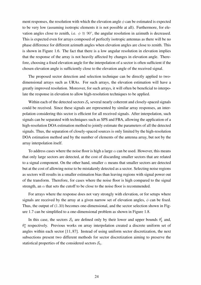
ment responses, the resolution with which the elevation angle φ can be estimated is expectedto be very low (assuming isotropic elements it is not possible at all). Furthermore, for ele-vation angles close to zenith, i.e. φ u 90◦, the angular resolution in azimuth is decreased.This is expected even for arrays composed of perfectly isotropic antennas as there will be nophase difference for different azimuth angles when elevation angles are close to zenith. Thisis shown in Figure 1.6. The fact that there is a low angular resolution in elevation impliesthat the response of the array is not heavily affected by changes in elevation angle. There-fore, choosing a fixed elevation angle for the interpolation of a sector is often sufficient if thechosen elevation angle is sufficiently close to the elevation angle of the received signal.
The proposed sector detection and selection technique can be directly applied to two-dimensional arrays such as URAs. For such arrays, the elevation estimation will have agreatly improved resolution. Moreover, for such arrays, it will often be beneficial to interpo-late the response in elevation to allow high-resolution techniques to be applied.
Within each of the detected sectors Sk several nearly coherent and closely-spaced signalscould be received. Since these signals are represented by similar array responses, an inter-polation considering this sector is efficient for all received signals. After interpolation, suchsignals can be separated with techniques such as SPS and FBA, allowing the application of ahigh-resolution DOA estimation method to jointly estimate the parameters of all the detectedsignals. Thus, the separation of closely-spaced sources is only limited by the high-resolutionDOA estimation method and by the number of elements of the antenna array, but not by thearray interpolation itself.
To address cases where the noise floor is high a large α can be used. However, this meansthat only large sectors are detected, at the cost of discarding smaller sectors that are relatedto a signal component. On the other hand, smaller α means that smaller sectors are detectedbut at the cost of allowing noise to be mistakenly detected as a sector. Selecting noise regionsas sectors will results in a smaller estimation bias than leaving regions with signal power outof the transform. Therefore, for cases where the noise floor is high compared to the signalstrength, an α that sets the cutoff to be close to the noise floor is recommended.
For arrays where the response does not vary strongly with elevation, or for setups wheresignals are received by the array at a given narrow set of elevation angles, φ can be fixed.Thus, the output of (1.30) becomes one-dimensional, and the sector selection shown in Fig-ure 1.7 can be simplified to a one-dimensional problem as shown in Figure 1.8.
In this case, the sectors Sk are defined only by their lower and upper bounds θlk and,θuk respectively. Previous works on array interpolation created a discrete uniform set ofangles within each sector [11, 87]. Instead of using uniform sector discretization, the nextsubsections present two different methods for sector discretization aiming to preserve thestatistical properties of the considered sectors Sk.
24
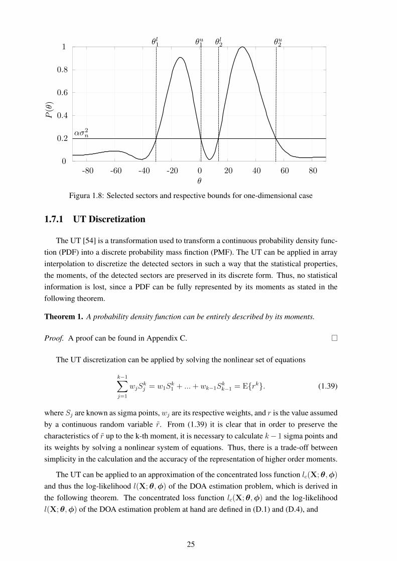
-80 -60 -40 -20 0 20 40 60 800
0.2
0.4
0.6
0.8
1
ασ2n
θl1 θu1 θl2 θu2
θ
P(θ)
Figura 1.8: Selected sectors and respective bounds for one-dimensional case
1.7.1 UT Discretization
The UT [54] is a transformation used to transform a continuous probability density func-tion (PDF) into a discrete probability mass finction (PMF). The UT can be applied in arrayinterpolation to discretize the detected sectors in such a way that the statistical properties,the moments, of the detected sectors are preserved in its discrete form. Thus, no statisticalinformation is lost, since a PDF can be fully represented by its moments as stated in thefollowing theorem.
Theorem 1. A probability density function can be entirely described by its moments.
Proof. A proof can be found in Appendix C.
The UT discretization can be applied by solving the nonlinear set of equations
k−1∑j=1
wjSkj = w1S
k1 + ...+ wk−1S
kk−1 = E{rk}. (1.39)
where Sj are known as sigma points, wj are its respective weights, and r is the value assumedby a continuous random variable r. From (1.39) it is clear that in order to preserve thecharacteristics of r up to the k-th moment, it is necessary to calculate k− 1 sigma points andits weights by solving a nonlinear system of equations. Thus, there is a trade-off betweensimplicity in the calculation and the accuracy of the representation of higher order moments.
The UT can be applied to an approximation of the concentrated loss function lc(X;θ,φ)
and thus the log-likelihood l(X;θ,φ) of the DOA estimation problem, which is derived inthe following theorem. The concentrated loss function lc(X;θ,φ) and the log-likelihoodl(X;θ,φ) of the DOA estimation problem at hand are defined in (D.1) and (D.4), and
25
θ = [θ1, . . . , θd]T, (1.40)
φ = [φ1, . . . , φd]T. (1.41)
Theorem 2. The concentrated loss function lc(X;θ,φ) for a DOA estimation problem canbe approximated for each detected sector Sk by the normalized power response of the con-ventional beamformer (1.30).
Proof. A proof can be found in Appendix D.
Following the approximation derived in Theorem 2 the concentrated loss function andthus the log-likelihood with respect to each sector Sk can be considered as a separate PDFeach when applying the UT. In order to preserve the first and the second moment of theapproximated log-likelihood, the number of points are chosen to transform each detectedsector Sk must be larger or equal than 3. Under this constraint and under the assumption thatthe input noise follows CN (0, σ2
n), the respective PDF characteristics for each sector Sk aremainly preserved. Figure 1.9 presents how the concentrated loss function lc(X;θ,φ) canbe represented using the UT for a linear array assuming uniform antenna responses of thedifferent antennas in elevation. A total transformation sector by concatenating all the sigmapoints given by the UT for the detected sectors can be written as
AS = [a(S1), a(S2), ..., a(ST )] ∈ CM×T , (1.42)
where T is the total number of points used to discretize all the detected sectors.
-80 -60 -40 -20 0 20 40 60 80
ω1, ω3
ω4, ω6
ω2
ω5
|w| S1
S2
S3
S4
S5
S6
θ
Figura 1.9: UT of the approximated lc(X;θ,φ) for two sources
The proposed UT-based discretization is well suited for linear arrays that have a uni-form response in elevation. The calculation of the sigma points St and weights ωt with
26
t = 1, . . . , T of the UT transformation is computationally expensive. Therefore, calculatingmultiple sets of points across multiple elevations may become infeasible depending on theapplication and system at hand. The UT can be very useful also when applying linear inter-polation, as it can be used to ensure that the least squares calculation of the transformationmatrix is a determined problem instead of an overdetermined one.
1.7.2 Principal Component Discretization
For most interpolation methods presented in the literature, the interpolated sectors arediscretized using a simple uniform discretization [11, 87]. The discretization is usually donesuch that the discrete angles are closely spaced. Therefore, the steering vectors of suchclosely spaced angles are highly correlated. This work proposes the application of principalcomponent analysis (PCA) to avoid problems caused by the correlation in predictors as wellas to minimize the computational load of the transformation.
Ideally, AS would be set up such that ASAHS = IM . However, as stated previously, this
is often not the case with ASAHS = RASAS 6= IM . PCA aims to find a matrix P such that
PAS = CS , (1.43)
where CSCHS = IM . P can be obtained by performing the eigendecomposition of RASAS
RASAS = EΣEH, (1.44)
and setting P = E. The transformation can then be calculated with respect to the transformedorthogonal dataset CS . The proposed PCA pre-processing can be used to create a better setof predictor variables for the interpolation and to reduce the dimensionality of the problemby excluding any eigenvectors associated to very small eigenvalues.
1.8 Linear Adaptive Array Interpolation
In the case of linear interpolation, the transformation bias is closely tied to the total sizeof the transformed sector. While the UT and PCA discretization can minimize this problem,they cannot fully mitigate it. Therefore, this thesis presents an iterative approach that seeksto find out the maximum region of the field of view that can be transformed while keepingthe transformation error bounded by a value. It also distributes the calculated region withrespect to the power of each sector detected in the second step.
The first part of the next two steps is to calculate a weighting factor based on the powerof each detected sector. This weighting factor will be used to optimally distribute the trans-formable region with respect to the received power, focusing the transformation on regionswith more power and aiming to leave the least significant power outside of the total trans-
27
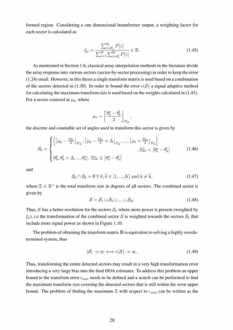
formed region. Considering a one dimensional beamformer output, a weighting factor foreach sector is calculated as
ξw =
∑θuwz=θlw
P [z]∑Wc=1
∑θucz=θlc
P [z]∈ R. (1.45)
As mentioned in Section 1.6, classical array interpolation methods in the literature dividethe array response into various sectors (sector-by-sector processing) in order to keep the error(1.24) small. However, in this thesis a single transform matrix is used based on a combinationof the sectors detected in (1.30). In order to bound the error ε(S) a signal adaptive methodfor calculating the maximum transform size is used based on the weights calculated in (1.45).For a sector centered at µk, where
µk =
⌈θuk − θlk
2
⌋D∆
,
the discrete and countable set of angles used to transform this sector is given by
Sk =
[⌈µk − Ξξk
2
⌋D∆
,⌈µk − Ξξk
2+ ∆
⌋D∆
, ...,⌈µk + Ξξk
2
⌋D∆
],Ξξk <
∣∣θuk − θlk∣∣[θlk, θ
lk + ∆, ..., θuk ], Ξξk ≥
∣∣θuk − θlk∣∣(1.46)
andSk ∩ Sk = ∅ ∀ k, k ∈ [1, ..., K] and k 6= k, (1.47)
where Ξ ∈ R+ is the total transform size in degrees of all sectors. The combined sector isgiven by
S = S1 ∪ S2 ∪ ... ∪ SK . (1.48)
Thus, S has a better resolution for the sectors Sk where more power is present (weighted byξk), i.e the transformation of the combined sector S is weighted towards the sectors Sk thatinclude more signal power as shown in Figure 1.10.
The problem of obtaining the transform matrix B is equivalent to solving a highly overde-termined system, thus
|S| → ∞ ⇐⇒ ε(S)→∞. (1.49)
Thus, transforming the entire detected sectors may result in a very high transformation errorintroducing a very large bias into the final DOA estimates. To address this problem an upperbound to the transform error εmax needs to be defined and a search can be performed to findthe maximum transform size covering the detected sectors that is still within the error upperbound. The problem of finding the maximum Ξ with respect to εmax can be written as the
28
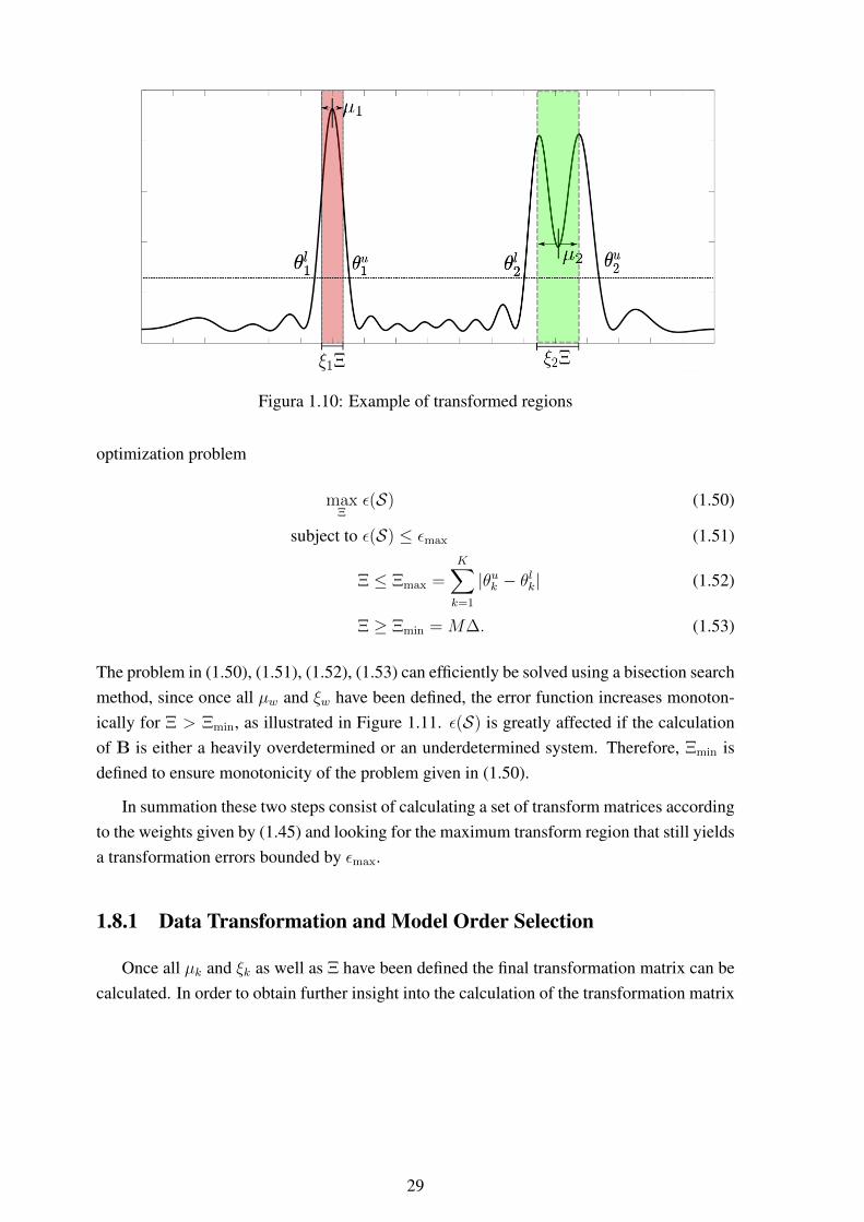
Brasil Hexa Champion!!!
Figura 1.10: Example of transformed regions
optimization problem
maxΞ
ε(S) (1.50)
subject to ε(S) ≤ εmax (1.51)
Ξ ≤ Ξmax =K∑k=1
|θuk − θlk| (1.52)
Ξ ≥ Ξmin = M∆. (1.53)
The problem in (1.50), (1.51), (1.52), (1.53) can efficiently be solved using a bisection searchmethod, since once all µw and ξw have been defined, the error function increases monoton-ically for Ξ > Ξmin, as illustrated in Figure 1.11. ε(S) is greatly affected if the calculationof B is either a heavily overdetermined or an underdetermined system. Therefore, Ξmin isdefined to ensure monotonicity of the problem given in (1.50).
In summation these two steps consist of calculating a set of transform matrices accordingto the weights given by (1.45) and looking for the maximum transform region that still yieldsa transformation errors bounded by εmax.
1.8.1 Data Transformation and Model Order Selection
Once all µk and ξk as well as Ξ have been defined the final transformation matrix can becalculated. In order to obtain further insight into the calculation of the transformation matrix
29
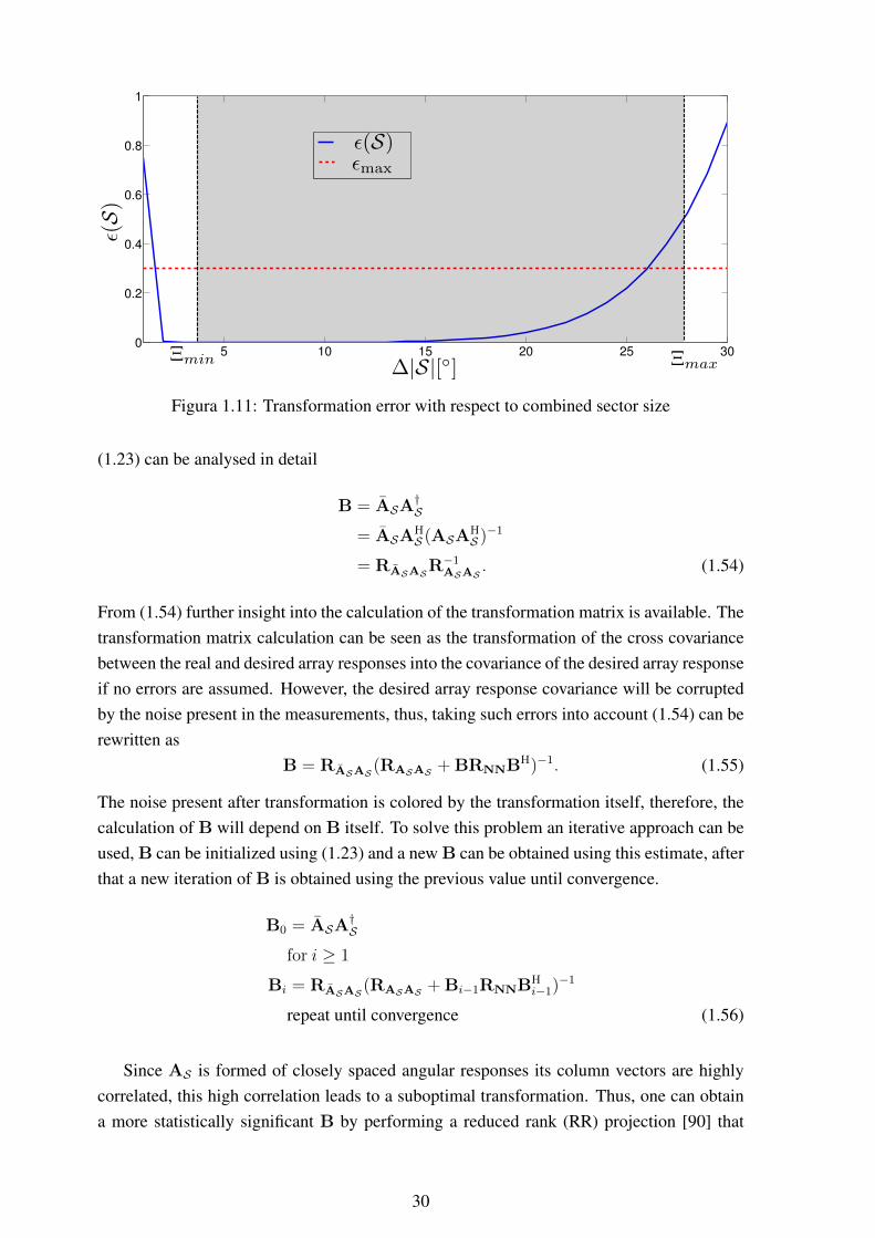
5 10 15 20 25 300
0.2
0.4
0.6
0.8
1
Figura 1.11: Transformation error with respect to combined sector size
(1.23) can be analysed in detail
B = ASA†S
= ASAHS (ASA
HS )−1
= RASASR−1ASAS
. (1.54)
From (1.54) further insight into the calculation of the transformation matrix is available. Thetransformation matrix calculation can be seen as the transformation of the cross covariancebetween the real and desired array responses into the covariance of the desired array responseif no errors are assumed. However, the desired array response covariance will be corruptedby the noise present in the measurements, thus, taking such errors into account (1.54) can berewritten as
B = RASAS (RASAS + BRNNBH)−1. (1.55)
The noise present after transformation is colored by the transformation itself, therefore, thecalculation of B will depend on B itself. To solve this problem an iterative approach can beused, B can be initialized using (1.23) and a new B can be obtained using this estimate, afterthat a new iteration of B is obtained using the previous value until convergence.
B0 = ASA†S
for i ≥ 1
Bi = RASAS (RASAS + Bi−1RNNBHi−1)−1
repeat until convergence (1.56)
Since AS is formed of closely spaced angular responses its column vectors are highlycorrelated, this high correlation leads to a suboptimal transformation. Thus, one can obtaina more statistically significant B by performing a reduced rank (RR) projection [90] that
30
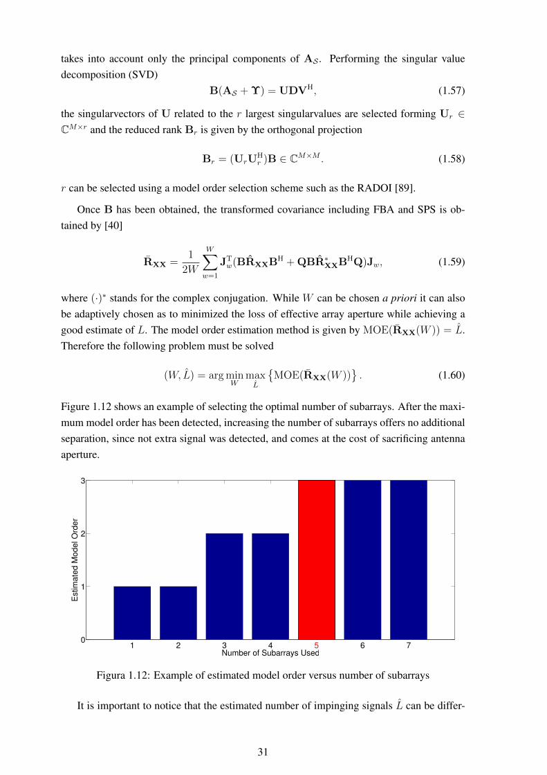
takes into account only the principal components of AS . Performing the singular valuedecomposition (SVD)
B(AS + Υ) = UDVH, (1.57)
the singularvectors of U related to the r largest singularvalues are selected forming Ur ∈CM×r and the reduced rank Br is given by the orthogonal projection
Br = (UrUHr )B ∈ CM×M . (1.58)
r can be selected using a model order selection scheme such as the RADOI [89].
Once B has been obtained, the transformed covariance including FBA and SPS is ob-tained by [40]
RXX =1
2W
W∑w=1
JTw(BRXXBH + QBR∗XXBHQ)Jw, (1.59)
where (·)∗ stands for the complex conjugation. While W can be chosen a priori it can alsobe adaptively chosen as to minimized the loss of effective array aperture while achieving agood estimate of L. The model order estimation method is given by MOE(RXX(W )) = L.Therefore the following problem must be solved
(W, L) = arg minW
maxL
{MOE(RXX(W ))
}. (1.60)
Figure 1.12 shows an example of selecting the optimal number of subarrays. After the maxi-mum model order has been detected, increasing the number of subarrays offers no additionalseparation, since not extra signal was detected, and comes at the cost of sacrificing antennaaperture.
1 2 3 4 5 6 70
1
2
3
Number of Subarrays Used
Est
imat
ed M
odel
Ord
er
Figura 1.12: Example of estimated model order versus number of subarrays
It is important to notice that the estimated number of impinging signals L can be differ-
31
ent from the number of sectors detected in (1.30). Each of the detected sectors Sk can beformed by a set of nearly coherent signals that now can be efficiently separated with (1.60)allowing the application of a high resolution DOA estimation method to jointly estimate theparameters of all the detected signals.
Its important to highlight now that if a ML method [84, 85] or its extensions such as theEM [32,77,79,82] or SAGE [33,38] would be chosen for estimating the direction of arrival ofthe received signals the model order would have to be estimated first, and to do so, in highlycorrelated signal environments, FBA and SPS need to be applied since model order selectionschemes rely on the analysis of the profile of the eigen or singular values. In practice, thismeans that even if a parametric ML method was to be used the steps taken so far into thealgorithm would still need to be taken. Therefore, no claims of increased complexity can bemade, up to this point, when the proposed DOA estimation algorithm is compared to a MLalgorithm and the presented steps of the proposed algorithm can be viewed as a separate partthat can be applied to use ML methods in highly correlated signals, arbitrary geometry arrayenvironments if one has no prior knowledge of the number of received signals.
1.8.2 Linear UT Array Interpolation
A linear transformation that takes into account the weights found by the UT for the sigmapoints can be found by extending (1.23), resulting in
BUT = ASUT
√diag{[w1, w2, ..., wM ]}AH
SUT(ASUT
√diag{[w1, w2, ..., wM ]}AH
SUT
)−1
∈ CM×M ,
(1.61)
where ASUTstands for the steering matrix of sector S after it has been discretized using the
UT.
Following the proposed approach the transformation error shown in (1.24) is zero. How-ever, the proposed approach requires the calculation of multiple sigma points through solvingnonlinear systems of equations, and, for setting up such systems, it is necessary to obtain themoments of the likelihoods truncated from the beamformer output. To simplify the applica-tion and allow the proposed method to be used in real-time array interpolation for systemswith limited processing power, this work proposes calculating sigma points for commonsector likelihoods, that is, defining a set of sigma points for common expected beamformerwaveforms that a real-time system may use. Using this set of points the interpolation matrixcan be calculated and stored in a look-up-table as signals are detected by the system as theinterpolation can them be applied.
The transformation matrix calculation can be seen as the transformation of the weighted
32

cross-covariance between the real and desired array responses into the covariance of thedesired array response. However, the desired array response covariance is corrupted by thenoise present in the measurements. The noise present after transformation is colored by thetransformation itself, therefore, the calculation of BUT will depend on BUT itself. To solvethis problem, an iterative approach can be used,
BUT(p) = ASUT
√diag{[w1, w2, ..., wM ]}AH
SUT((ASUT
√diag{[w1, w2, ..., wM ]}AH
SUT
)+ B
(p−1)UT RNNB
(p−1)HUT
)−1
∈ CM×M , (1.62)
where B(0)UT can be initialized using a diagonal RNN with σ2
n filling its diagonal. After that anew iteration of B
(p)UT is obtained using the previous value until convergence.
1.9 Multidimensional Linear Interpolation
This section extends the concepts of linear interpolation to arrays of two or more dimen-sions.
1.9.1 Tensor Algebra Concepts
This section introduces the tensor algebra concepts of tensor unfolding and r-mode prod-uct.
1.9.1.1 Tensor Unfolding
In order to operate with tensors using well-know linear algebra tools via the applicationof tensor unfoldings. This operation transforms a tensor of dimension R > 2 into a matrix.The r-mode unfolding of tensor A is denoted by
[A](r) ∈ CMr×(M1·M2·...·Mr−1·Mr+1·...·MR). (1.63)
[A](r) is a matrix containing the r-mode vectors or r fibers of tensor A along its rows. Ar-mode vector can be obtained by fixing the index of all dimensions other than r and varyingthe index of the r-th dimension along its range.
The unfoldings of the tensor presented in Figure 1.13 are given by
[B](1) =
[1 3 5 7
2 4 6 8
], (1.64)
33

B = 1
2
3
4
5
6
7
8
Figura 1.13: Tensor B ∈ R2×2×2
[B](2) =
[1 2 5 6
3 4 7 8
], (1.65)
[B](3) =
[1 2 3 4
5 6 7 8
]. (1.66)
1.9.1.2 r-Mode Product
The r-mode product of a tensor A ∈ CM1×M2×...×Mr and a matrix D ∈ CL×Mr is denoteby
C = A×r D ∈ CM1×M2×...×L×...×Mr , (1.67)
which is equivalent to[A×r D] = D · [A](r). (1.68)
Thus, the matrix D must have the same number of columns as the numbers of elements inthe r-th dimension of A.
1.9.2 Multidimensional Data Model
The data model consider d planar wavefronts are impinging on an antenna array contain-ing M1 ×M2 × ... ×MR elements. The signal received at the m1,m2, . . .mR antenna at agiven time snapshot t is given by
xm1,m2,...mR,t =d∑i=1
γm1,m2,...mR,dsi[n]R∏r=1
ej·(mr−1)·µ(r)i
+nm1,m2,...mR,n, (1.69)
where si[n] is the complex symbol transmitted by the i-th source at time snapshot n,nm1,m2,...mR,t is the zero mean circularly symmetric (ZMCS) white complex Gaussian noisepresent at antenna m1,m2, . . .mR at time snapshot n. γm1,m2,...mR is an imperfection presentat the antenna m1,m2, . . .mR. µ(r)
i represents the spatial frequency of the signal transmittedby the i-th source over the r-th dimension, note that the spatial frequency can be mapped intodifferent parameters depending on the dimension. In case of spatial dimension, it is mapped
34

into a direction of arrival, while for frequency and time dimensions it can be mapper intotime delay of arrival and Doppler shift, respectively.
For the received signal to have the PARAFAC structure its steering array must havea Khatri-Rao structure as follows. Let Mr be the size of the r-th dimension, and M =∏R
r=1 Mr. A steering vector a(r)i containing the spatial frequencies relate to the i-th source
over the r-th dimension can be defined as
a(r)i =
[1 ej·µ
(r)i · · · e(Mr−1)·j·µ(r)
i
]T
. (1.70)
Therefore, an array steering vector for the i-th source can be written as
ai = a(1)i ⊗ a
(2)i ⊗ . . .⊗ a
(r)i ∈ CM×1, (1.71)
while the array steering matrix for the r-th dimension can be constructed as
A(r) =[a
(r)1 , a
(r)2 , . . . , a
(r)d
]∈ CM×d. (1.72)
Finally, the total steering matrix of the d sources can be constructed in terms of Khatri-Raoproducts of all array steering matrices of all dimensions.
A = A(1) �A(2) � . . . �A(r) ∈ CM×d. (1.73)
For the tensor notation, a PARAFAC steering tensor for each of the d signal sources canbe obtained by
Ai = a(1)i ◦ a
(2)i ◦ . . . ◦ a
(r)i ∈ CM1×M2×···×MR , (1.74)
where ◦ is the outer product. A total array steering tensor can be constructed by concatenat-ing the individual steering tensor for each of the signal sources over the r + 1 dimension, asit follows
A =[A1|R+1A2|R+1 . . . |R+1Ad] ∈ CM1×M2×···×MR×d. (1.75)
The |r operator represents the concatenation operation over the r-th dimension.
A non PARAFAC steering tensor can be written as
X = (A� G)×R ST +N ,∈ CM1×M2×...×MR×N , (1.76)
here N ∈ CM1×M2×...×MR×N is the noise tensor and contains the noise samples interfer-ing with the measurements, and G ∈ CM1×M2×···×MR×d is a tensor containing the antennaimperfections.
35
1.9.3 Multidimensional Interpolation
Array interpolation can be extended to the multidimensional case by considering themultidimensional data model and rewriting (1.19) as
I ×1 A1 ×2 A2...×R AR = A×1 B1 ×2 B2...×R BR, (1.77)
where Ar is the desired array response for the r-th dimension and Br is the transformationmatrix for the r-th dimension given by
Br = [A](r)A†r, (1.78)
where (�)† stands for the Moore–Penrose pseudo-inverse. Note that in this case the originalarrayA has no PARAFAC structure, while the array after the interpolation has the PARAFACstructure.
Similar to what is done in the matrix case, the power response is used to the detect sectorsfor interpolation. The power response for dimension r is given by
P (µ(r)) =
∣∣∣∣∣w(r)H(µ(r))R(r)XXw(r)(µ(r))
w(r)H(µ(r))w(r)(µ(r))
∣∣∣∣∣ ∈ R, (1.79)
where (·)H is the conjugate hermitian and R(r)XX is the spatial covariance matrix for dimension
(r). R(r)XX is given by
R(r)XX =
Mr
N∏R
i=1 Mi
[X ](r)[X ]H(r) ∈ CMr×Mr . (1.80)
Following the matrix approach, the output of (1.79) is scanned for K sectors, and foreach sector the respective lower bound l(r)k ∈ D∆ and upper bound u(r)
k ∈ D∆, where k =
1, . . . , K, are defined done in the matrix case. If K sectors are detected, a detected sectorwith bounds [l
(r)k , u
(r)k ] is said to be centred at
ck =
∣∣∣u(r)k − l
(r)k
∣∣∣2
D∆
∈ D∆, (1.81)
After the sectors are detected for each of the dimensions, they can be discretized and atransformation can be calculated following the same steps presented for the one dimensionalcase. After Br has been obtained for all the dimensions to be interpolated the received datacan be transformed by
X ×1 B1 ×2 B2 . . .×R BR. (1.82)
The transformation also affects the noise component, leading to coloured noise at the output.This requires some sort of prewhitening to be applied prior to some DOA estimation algo-
36
rithms. For prewhitening schemes, the reader may refer to [26] for the matrix case and [25]for the tensor case.
Depending on the structure chosen for the interpolated array many different DOA estima-tion methods can be applied. Multidimensional ESPRIT approaches such as [48] or methodsbased on the PARAFAC decomposition such as [29], [28] can be used.
1.10 Nonlinear Array Interpolation
In this section two nonlinear alternatives to array interpolation, allowing the applicationof FBA and SPS in highly correlated signal scenarios, are presented. Subsection 1.10.1presents an interpolation approach based on the MARS regression method, allowing a modelto be created expressing nonlinear relationships between the true and the desired array re-sponse. Subsection 1.10.2 shows an interpolation approach based on GRNNs, this approachcan be implemented in a parallel manner, making it a good candidate for array interpolationunder real-time constraints. For the nonlinear approaches sector selection and discretizationcan be perform identically to when linear approaches are employed.
1.10.1 MARS based interpolation
This work proposes a nonlinear interpolation method based on the MARS technique. TheMARS regression approach is detailed in Appendix E. The proposed interpolation approachbuilds a mapping that splits the real and imaginary parts of the response of each of theantennas of the array, that is, a total of 2M MARS models are built to interpolate the arrayresponse with respect to the combined sector S. Based on (E.4) this mapping can be writtenas
∀ (θ, φ) ∈ S :
[<{a(θ, φ)}={a(θ, φ)}
]= f (a(θ, φ))
=
∑LR1`=1 c
R`,1F
R`,1 (<{a(θ, φ)})...∑LRM
`=1 cR`,MF
R`,M (<{a(θ, φ)})∑LI1
`=1 cI`,1F
I`,1 (={a(θ, φ)})...∑LIM
`=1 cI`,MF
I`,M (={a(θ, φ)})
, (1.83)
where cRlm and cIlm are the weighting constants, FRlm
and F Ilm
are the basis functions and LRmand LIm are the number of functions and weighting constants of each model. Furthermore,<{a(θ, φ)} and={a(θ, φ)} denote the real and imaginary part of vector a(θ, φ), respectively.Based on (E.6) the generalized cross-validation (GCV) for the backward pass (step used to
37
reduce possible over-fitting of the model) can be written as
<{GCV} =
1|S|∑
(θ,φ)∈S(<{a[m](θ, φ)} − fRm(a(θ, φ)))2
(1− LRm+pLRm−1
2
|S| )2
, (1.84)
={GCV} =
1|S|∑
(θ,φ)∈S(={a[m](θ, φ)} − f Im(a(θ, φ)))2
(1− LIm+pLIm−1
2
|S| )2
, (1.85)
where fRm and f Im are the real and imaginary part of the model for the m-th antenna, re-spectively. Both <{GCV} and <{GCV} are used to avoid over-fitting, that is, to reducethe complexity of the model created in order to avoid fitting of the noise or of measure-ment errors of the array response. a[m](θ, φ) denotes the m-th element of the virtual arrayresponse. To use this approach in an real-time system the models can be built in an initializa-tion step. Sectors of interest for the application of the MARS interpolation can be selectedand a model can be built and stored as a look-up table. The data received can be interpolatedsnapshot-wise with [
<{x[n]}={x[n]}
]= f (x[n]) , (1.86)
where x[n] ∈ CM×1 is the n -th column of matrix X with n = 1, . . . , N .
In some cases, the antenna array will have a response which is similar enough to thedesired response in some of its field of view so that a linear approach yields good results.Thus, the MARS approach can be used only on portions of the field of view where the realresponse differs strongly from the desired one.
The MARS approach is especially useful for arrays with a small number of elements. Forlinear approaches, the degrees of freedom of the linear approach are limited by the numberof antennas in the virtual array. It is possible to increase the degrees of freedom by creatinga virtual array with a larger number of antennas, however, this will lead to a transformationmatrix that is ill-conditioned and results in a large bias in the DOA estimates. The MARSapproach, on the other hand, can build as many hinge functions and relationships betweenthem as necessary.
1.10.2 GRNN based interpolation
GRNNs are a type of neural network used for general regression problems that are ex-tended in this work for the problem of array interpolation. An overview of GRNNs is pre-sented in Appendix F.
Classic interpolation relies on transforming an array response over the discrete set ofangles S. In linear array interpolation, the choice of points that belong to S is usually anarbitrary one, based solely on the predefined sector bounds and the chosen angular resolu-
38
tion. When applying a linear approach, angular resolution is usually chosen to be as high aspossible, thus, the set of points belonging to S is usually closely spaced. This is not neces-sary when applying the GRNN since it is capable of interpolating between multiple sets oftraining data. In fact, a dense set of training points will result in an increased computationalload while providing very little benefit to the overall accuracy of the GRNN based arrayinterpolation.
The neural network representing the real and imaginary parts of the array can be built byextending (F.1) and (F.2) to the application at hand, resulting in the mapping[
<{x[n]}={x[n]}
]= f (x[n], a(θ, φ), a(θ, φ)) , (1.87)
and
<{x[m][n]} =
∑(θ,φ)∈S <{a[m](θ, φ)}e−
ξ(θ,φ)
2σ2∑(θ,φ)∈S e
− ξ(θ,φ)
2σ2
, (1.88)
={x[m][n]} =
∑(θ,φ)∈S ={a[m](θ, φ)}e−
ξ(θ,φ)
2σ2∑(θ,φ)∈S e
− ξ(θ,φ)
2σ2
, (1.89)
where σ2 is the smoothness parameter, and
ξ(θ, φ) = ||x[n]− a(θ, φ)||22. (1.90)
Once the data has been interpolated to the desired array structure, array signal processingschemes such as FBA, SPS or ESPRIT can be applied. Differently, from other array in-terpolation methods, there is no noise color introduced by the interpolation, therefore pre-whitening is not necessary.
One of the advantages of applying GRNNs to array interpolation is that the sectors con-sidered for transformation can be made very large while having a small effect on the accuracyof the interpolation. As shown in (1.88, 1.89), in case the input resembles the data used forthe training in a certain region of the transformed sector, this data will have a larger weight.On the other hand, if the input is distant from any region of the transformed sector, this regionwill have very little influence on the output of the interpolation.
Therefore, with a GRNN it is possible to transform very large regions of the field of viewof the array without suffering from the same problems as the ones present in linear arrayinterpolation, where the transformation error grows as the transformed region grows. On theother hand, transforming a large region using the GRNN will increase the computational costof the interpolation. As shown in Figure F.1 it is possible to implement the proposed GRNNarray interpolation in a parallel manner, leading to a faster interpolation. Thus, the proposedGRNN array interpolation is a possible alternative for precise array interpolation in real-time
39
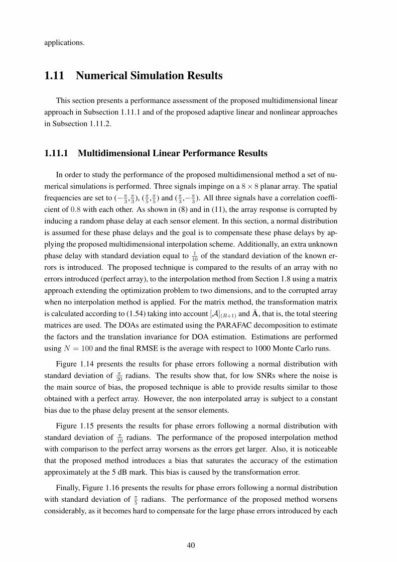
applications.
1.11 Numerical Simulation Results
This section presents a performance assessment of the proposed multidimensional linearapproach in Subsection 1.11.1 and of the proposed adaptive linear and nonlinear approachesin Subsection 1.11.2.
1.11.1 Multidimensional Linear Performance Results
In order to study the performance of the proposed multidimensional method a set of nu-merical simulations is performed. Three signals impinge on a 8× 8 planar array. The spatialfrequencies are set to (−π
3,π3), (π
5,π5) and (π
3,−π
3). All three signals have a correlation coeffi-
cient of 0.8 with each other. As shown in (8) and in (11), the array response is corrupted byinducing a random phase delay at each sensor element. In this section, a normal distributionis assumed for these phase delays and the goal is to compensate these phase delays by ap-plying the proposed multidimensional interpolation scheme. Additionally, an extra unknownphase delay with standard deviation equal to 1
10of the standard deviation of the known er-
rors is introduced. The proposed technique is compared to the results of an array with noerrors introduced (perfect array), to the interpolation method from Section 1.8 using a matrixapproach extending the optimization problem to two dimensions, and to the corrupted arraywhen no interpolation method is applied. For the matrix method, the transformation matrixis calculated according to (1.54) taking into account [A](R+1) and A, that is, the total steeringmatrices are used. The DOAs are estimated using the PARAFAC decomposition to estimatethe factors and the translation invariance for DOA estimation. Estimations are performedusing N = 100 and the final RMSE is the average with respect to 1000 Monte Carlo runs.
Figure 1.14 presents the results for phase errors following a normal distribution withstandard deviation of π
20radians. The results show that, for low SNRs where the noise is
the main source of bias, the proposed technique is able to provide results similar to thoseobtained with a perfect array. However, the non interpolated array is subject to a constantbias due to the phase delay present at the sensor elements.
Figure 1.15 presents the results for phase errors following a normal distribution withstandard deviation of π
10radians. The performance of the proposed interpolation method
with comparison to the perfect array worsens as the errors get larger. Also, it is noticeablethat the proposed method introduces a bias that saturates the accuracy of the estimationapproximately at the 5 dB mark. This bias is caused by the transformation error.
Finally, Figure 1.16 presents the results for phase errors following a normal distributionwith standard deviation of π
5radians. The performance of the proposed method worsens
considerably, as it becomes hard to compensate for the large phase errors introduced by each
40
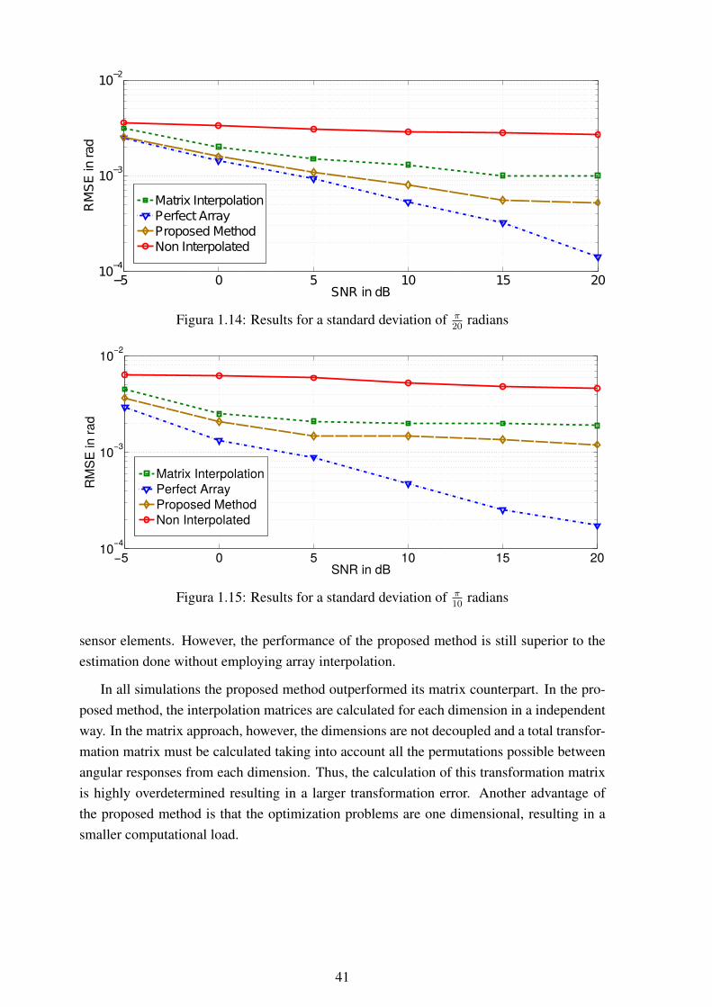
−5 0 5 10 15 2010
−4
10−3
10−2
SNR in dB
RM
SE
in rad
Matrix Interpolation
Perfect Array
Proposed Method
Non Interpolated
Figura 1.14: Results for a standard deviation of π20
radians
−5 0 5 10 15 2010
−4
10−3
10−2
SNR in dB
RM
SE
inra
d
Matrix Interpolation
Perfect Array
Proposed Method
Non Interpolated
Figura 1.15: Results for a standard deviation of π10
radians
sensor elements. However, the performance of the proposed method is still superior to theestimation done without employing array interpolation.
In all simulations the proposed method outperformed its matrix counterpart. In the pro-posed method, the interpolation matrices are calculated for each dimension in a independentway. In the matrix approach, however, the dimensions are not decoupled and a total transfor-mation matrix must be calculated taking into account all the permutations possible betweenangular responses from each dimension. Thus, the calculation of this transformation matrixis highly overdetermined resulting in a larger transformation error. Another advantage ofthe proposed method is that the optimization problems are one dimensional, resulting in asmaller computational load.
41
−5 0 5 10 15 2010
−4
10−3
10−2
10−1
SNR in dB
RM
SE
in
ra
ds
Matrix Interpolation
Perfect Array
Proposed Method
Non Interpolated
Figura 1.16: Results for a standard deviation of π5
radians
1.11.2 Nonlinear Performance Results
The performance of the proposed algorithms is tested considering a manufactured 6× 1
linear antenna array shown in Figure 1.17 [15]. The single antennas are circularly polarizeddielectric resonator antennas (DRA) [14], exhibiting a strong miniaturization of the aper-ture. The antennas are tuned to work at GPS L1 frequency band centered around 1575.42MHz in standalone configuration. Once in the array, no attempt has been made to re-tunethem, in order to emphasize the mutual coupling effects and eventual degradation. This6 × 1 linear array was especially designed for research on mutual coupling with adjustableinter-element spacing of the 6 antennas. The small dimensions of the single antennas allowto place them quite close to each other, up to a minimum distance of 30 mm (≈ 0.16λ atL1 central frequency). The following simulations consider array responses of the manufac-tured array measured in an anechoic chamber as well as array responses simulated using a3D electromagnetic simulator (ANSYS HFSS). Thus, realistic assessment of the proposedalgorithms can be achieved considering measured and properly simulated array responses.
The simulations are performed considering the receiver has no previous knowledge of thereceived signal. The combined sector is detected and discretized according to the methodspresented in Section 1.7. After discretization the combined sector is interpolated using thelinear and nonlinear methods proposed in Sections 1.7 and 1.10. The model order of theinterpolated data then is estimated by applying FBA and SPS adaptively and using RADOI[89] as the model order estimation method following the procedure proposed in [72]. Oncemodel order is estimated the DOA estimates are obtained using TLS-ESPRIT [91].
For obtaining RXX N = 100 snapshots are used and the Root Mean Squared Error(RMSE) is calculated with respect to 1000 Monte Carlo simulations. Two signals fromθ1 = 45◦ and θ2 = 15◦ with σ2
1 = σ22 = 1 and γ1,2 = 1 according to (1.4) are impinging on
42
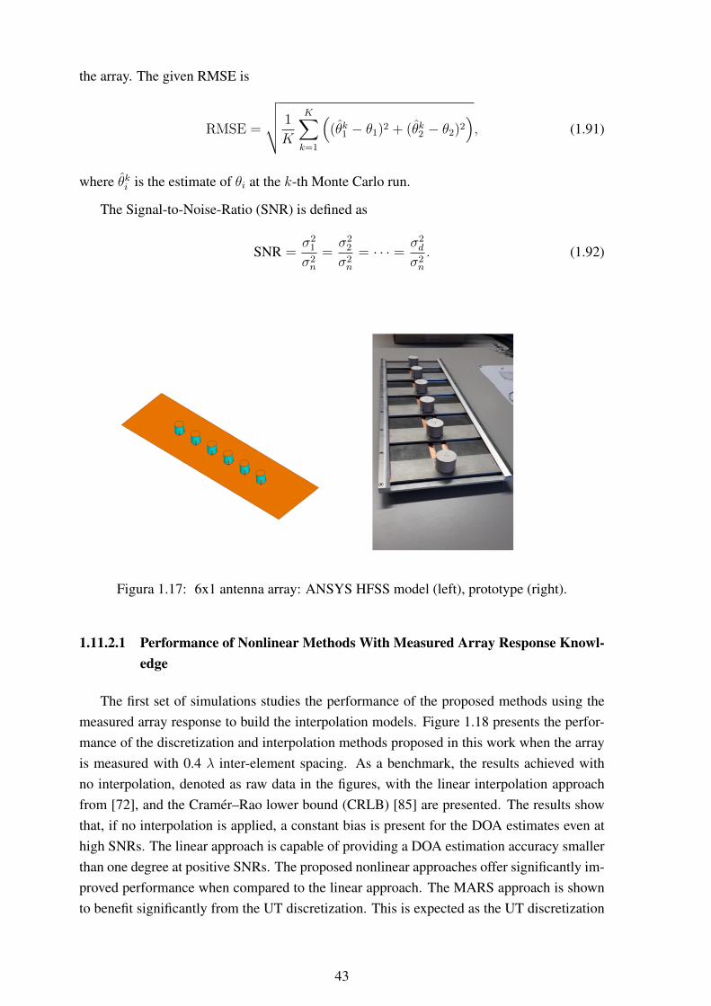
the array. The given RMSE is
RMSE =
√√√√ 1
K
K∑k=1
((θk1 − θ1)2 + (θk2 − θ2)2
), (1.91)
where θki is the estimate of θi at the k-th Monte Carlo run.
The Signal-to-Noise-Ratio (SNR) is defined as
SNR =σ2
1
σ2n
=σ2
2
σ2n
= · · · = σ2d
σ2n
. (1.92)
Figura 1.17: 6x1 antenna array: ANSYS HFSS model (left), prototype (right).
1.11.2.1 Performance of Nonlinear Methods With Measured Array Response Knowl-edge
The first set of simulations studies the performance of the proposed methods using themeasured array response to build the interpolation models. Figure 1.18 presents the perfor-mance of the discretization and interpolation methods proposed in this work when the arrayis measured with 0.4 λ inter-element spacing. As a benchmark, the results achieved withno interpolation, denoted as raw data in the figures, with the linear interpolation approachfrom [72], and the Cramér–Rao lower bound (CRLB) [85] are presented. The results showthat, if no interpolation is applied, a constant bias is present for the DOA estimates even athigh SNRs. The linear approach is capable of providing a DOA estimation accuracy smallerthan one degree at positive SNRs. The proposed nonlinear approaches offer significantly im-proved performance when compared to the linear approach. The MARS approach is shownto benefit significantly from the UT discretization. This is expected as the UT discretization
43
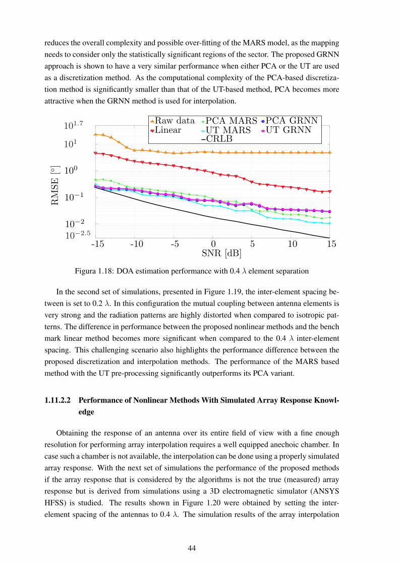
reduces the overall complexity and possible over-fitting of the MARS model, as the mappingneeds to consider only the statistically significant regions of the sector. The proposed GRNNapproach is shown to have a very similar performance when either PCA or the UT are usedas a discretization method. As the computational complexity of the PCA-based discretiza-tion method is significantly smaller than that of the UT-based method, PCA becomes moreattractive when the GRNN method is used for interpolation.
-15 -10 -5 0 5 10 15
10−2
10−1
Raw dataLinear
PCA MARSUT MARS
PCA GRNNUT GRNN
CRLB
100
101
SNR [dB]
RMSE
[◦]
101.7
10−2.5
Figura 1.18: DOA estimation performance with 0.4 λ element separation
In the second set of simulations, presented in Figure 1.19, the inter-element spacing be-tween is set to 0.2 λ. In this configuration the mutual coupling between antenna elements isvery strong and the radiation patterns are highly distorted when compared to isotropic pat-terns. The difference in performance between the proposed nonlinear methods and the benchmark linear method becomes more significant when compared to the 0.4 λ inter-elementspacing. This challenging scenario also highlights the performance difference between theproposed discretization and interpolation methods. The performance of the MARS basedmethod with the UT pre-processing significantly outperforms its PCA variant.
1.11.2.2 Performance of Nonlinear Methods With Simulated Array Response Knowl-edge
Obtaining the response of an antenna over its entire field of view with a fine enoughresolution for performing array interpolation requires a well equipped anechoic chamber. Incase such a chamber is not available, the interpolation can be done using a properly simulatedarray response. With the next set of simulations the performance of the proposed methodsif the array response that is considered by the algorithms is not the true (measured) arrayresponse but is derived from simulations using a 3D electromagnetic simulator (ANSYSHFSS) is studied. The results shown in Figure 1.20 were obtained by setting the inter-element spacing of the antennas to 0.4 λ. The simulation results of the array interpolation
44
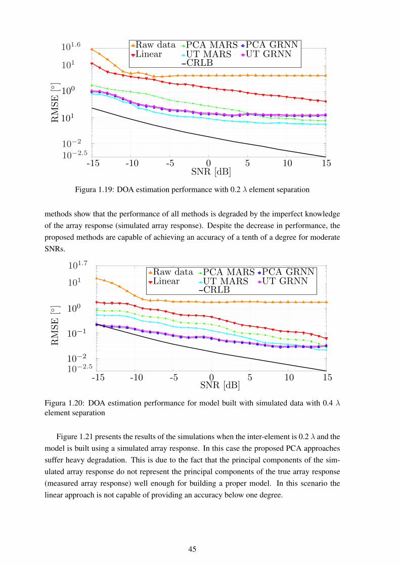
-15 -10 -5 0 5 10 15
Raw dataLinear
PCA MARSUT MARS
PCA GRNNUT GRNN
CRLB
10−2
101
100
101RMSE
[◦]
SNR [dB]
101.6
10−2.5
Figura 1.19: DOA estimation performance with 0.2 λ element separation
methods show that the performance of all methods is degraded by the imperfect knowledgeof the array response (simulated array response). Despite the decrease in performance, theproposed methods are capable of achieving an accuracy of a tenth of a degree for moderateSNRs.
-15 -10 -5 0 5 10 15
10−2
10−1
100
101
RMSE
[◦]
SNR [dB]
Raw dataLinear
PCA MARSUT MARS
PCA GRNNUT GRNN
CRLB
101.7
10−2.5
Figura 1.20: DOA estimation performance for model built with simulated data with 0.4 λelement separation
Figure 1.21 presents the results of the simulations when the inter-element is 0.2 λ and themodel is built using a simulated array response. In this case the proposed PCA approachessuffer heavy degradation. This is due to the fact that the principal components of the sim-ulated array response do not represent the principal components of the true array response(measured array response) well enough for building a proper model. In this scenario thelinear approach is not capable of providing an accuracy below one degree.
45
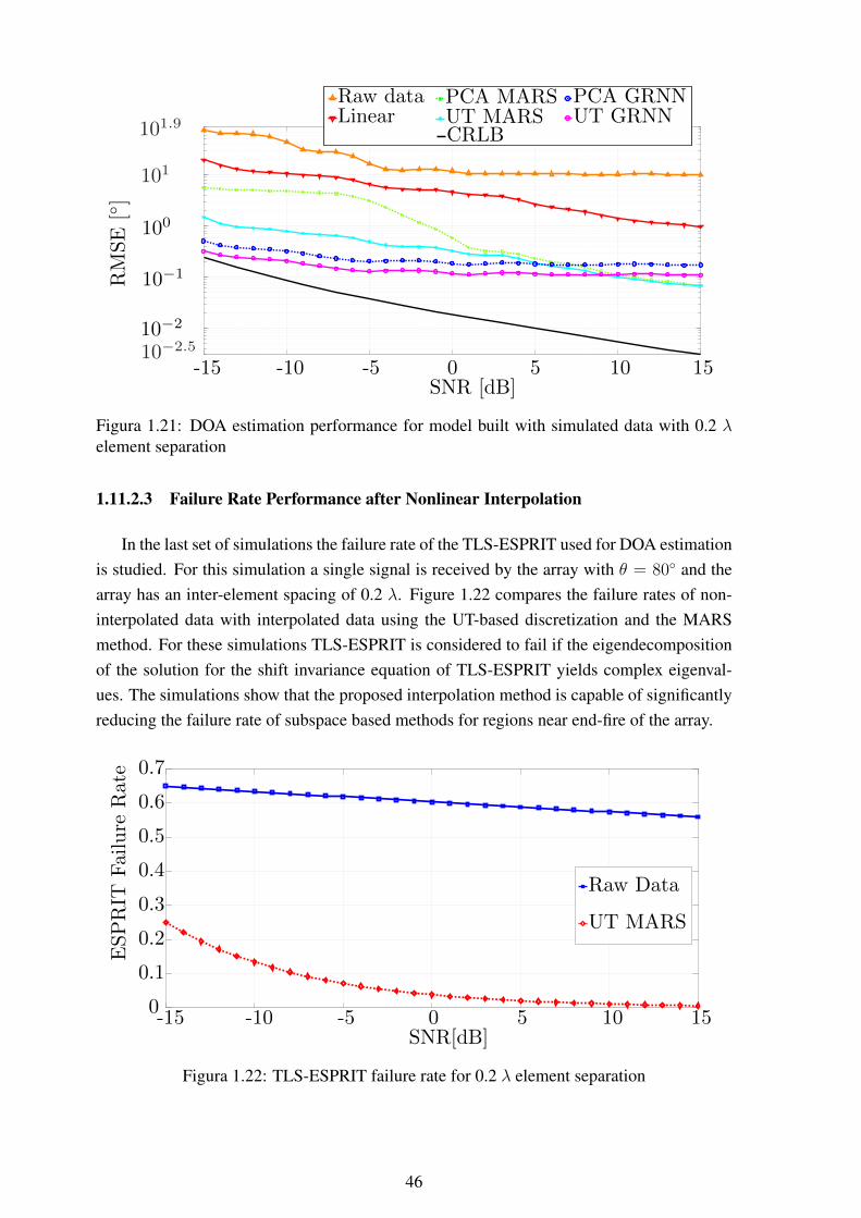
-15 -10 -5 0 5 10 15
10−2
10−1
100
101
RMSE
[◦]
SNR [dB]
Raw dataLinear
PCA MARSUT MARS
PCA GRNNUT GRNN
CRLB101.9
10−2.5
Figura 1.21: DOA estimation performance for model built with simulated data with 0.2 λelement separation
1.11.2.3 Failure Rate Performance after Nonlinear Interpolation
In the last set of simulations the failure rate of the TLS-ESPRIT used for DOA estimationis studied. For this simulation a single signal is received by the array with θ = 80◦ and thearray has an inter-element spacing of 0.2 λ. Figure 1.22 compares the failure rates of non-interpolated data with interpolated data using the UT-based discretization and the MARSmethod. For these simulations TLS-ESPRIT is considered to fail if the eigendecompositionof the solution for the shift invariance equation of TLS-ESPRIT yields complex eigenval-ues. The simulations show that the proposed interpolation method is capable of significantlyreducing the failure rate of subspace based methods for regions near end-fire of the array.
-15 -10 -5 0 5 10 150
0.1
0.2
0.3
0.4
0.5
0.6
0.7
Raw Data
ESPRIT
Failure
Rate
UT MARS
SNR[dB]
Figura 1.22: TLS-ESPRIT failure rate for 0.2 λ element separation
46
1.12 Summary
This chapter presented multiple array interpolation algorithms with the goal of allowinglow bias DOA estimation to be performed.
The first step is to detect sectors of interest, to this end a method for signal adaptivesector selection was presented. The proposed method scans the field of view of the arrayto detect and determine the sectors of interest for interpolation. Once the sectors have beendetected they must be discretized before being transformed, in this chapter two alternativesfor sector discretization, relying on the UT and the PCA were presented. These discretizationmethods are capable of discretizing the sector while maintaining the statistical integrity ofthe transformed data.
An adaptive linear approach for array interpolation was presented, aiming at minimizingthe transformation bias with respect to the received signal. This approach was extended tomultilinear arrays of arbitrary dimensions.
Nonlinear approaches have also been presented for the cases where the real array re-sponse deviates too heavily from the desired array response. A nonlinear interpolationmethod based on the MARS regression was presented capable of achieving good perfor-mance at moderate to high SNRs. A second nonlinear interpolation approach applyingGRNNs was presented, with a reduced computational complexity when compared to theMARS method, the GRNN method was shown to provide the best performance under lowSNR scenarios.
The efficiency of the proposed methods was tested by means of numerical simulationsusing a linear array with responses measured in an anechoic chamber as well as responsessimulated in a 3D electromagnetic simulator (ANSYS HFSS), tanking into account into ac-count all realistic effects, such as mutual coupling between the elements, and non-perfectradiation patterns. Furthermore, simulations were performed using real measured array pat-terns, validating the performance of the proposed methods under real life conditions.
The methods were capable of accurate DOA estimation and reduced the estimation biaswhen compared to a noninterpolated array. Linear estimation, while offering the worst per-formance among the methods presented, has a very low complexity. Nonlinear estimationmethods can offer improved performance when needed, at the cost of greatly increased com-putational complexity.
47

Chapter 2
Cooperative MIMO for Wireless SensorNetworks
In this chapter the following research question is addressed:Can array processing techniques be used to provide improved lifetime and communicationperformance in wireless sensor network?
2.1 Overview and Contribution
The remainder of this section is organized as follows:
• Motivation: An introduction to wireless sensor networks and how the challenges theyface can be addressed using array processing is presented in this section.
• Wireless Sensor Networks Organization: This section presents a brief descriptionof the usual organization inside WSNs
• Cooperative MIMO: Here, the concept of Cooperative MIMO (C-MIMO) is detailed.The mathematical model behind MIMO is addressed and the steps involved in per-forming MIMO over a distributed set of devices are presented.
• Energy Analysis: In this section the energy consumption of single-hop, multi-hopand C-MIMO communications is studied. The threshold for when to switch betweendifferent communication techniques is derived to maximize the energy efficiency withrespect to the distance involved in the communication.
• Synchronization: Here, the critical problem of synchronization for a distributedMIMO system is studied. The effects of synchronization errors in the performanceof MIMO transmissions is analysed. Two different methods for synchronization arepresented as detailed, allowing for different trade-offs between precision and compu-tational complexity. The error propagation involved in the synchronization of nodes
48

over multiple hops is also addressed. Finally, a closed formula for the minimum resyn-chronization interval with respect to clock drift and symbol duration is derived.
• Adaptive C-MIMO Clustering: This section presents an approach for adaptivelyforming C-MIMO communication clusters based on the distance involved in the com-munication and on the energy reserves of neighbouring nodes. This approach seeks tomaximize the energy efficiency of communications in the network while keeping theenergy distribution between the nodes as even as possible.
The research contributions presented in this chapter are:
1. A study on the energy efficiency of C-MIMO with respect to multi and single-hopcommunications, defining a threshold of selection between the multiple communica-tion techniques.
2. An analysis on the impact of synchronization errors in distributed MIMO system withrespect to the symbol period and the size of the communication clusters involved.
3. A study on the propagation of synchronization errors inside a WSN, and from thatthe derivation of a closed form expression regarding the resynchronization interval indistributed MIMO systems that takes into account the symbol duration and the clockdrift of the nodes involved.
4. Two methods for synchronization for WSNs with different trade-offs between perfor-mance and computational complexity.
5. An adaptive method for selecting the cluster size of C-MIMO transmissions capableof maximizing energy efficiency and improve the homogeneity of the energy reservesacross the network.
2.2 Motivation
Recent advances in electronics and miniaturization have allowed the development ofsmall, low-powered and low-cost devices capable of small range communication, a lim-ited amount of processing and of collecting data about its surroundings. Wireless sensornetworks (WSNs) are a collection of such devices, called nodes, organized in a cooperativenetwork environment. They possess various advantages over traditional sensor applications.Due to their low cost and small size they can be deployed densely and randomly to moni-tor a certain phenomenon. On the other hand, traditional sensors usually require extensiveplanning in their deployment and, depending on the nature of the phenomenon to be sensed,cannot be placed near it due to their high cost. WSNs are usually self-contained and capableof organizing the network on the fly. Due to this characteristics, these networks are suitablefor deployment on harsh environments.
49

WSN usage ranges from military applications, such as battlefield surveillance and target-ing, to healthcare applications, such as portable automated drug infusion systems in hospi-tals [1]. However, the extensive use of WSNs is still being hindered by the limited energybudget available in the nodes that constitute the networks. Furthermore, since WSNs aredeployed even in harsh and hard-to-reach environments, replacing individual nodes, or theirbatteries, is not always practical. Therefore, extensive research is being performed to maxi-mize the energy efficiency of WSNs [34].
Solutions for minimizing energy consumption in WSNs have been proposed through dif-ferent layers by analyzing energy efficiency for all the tasks involved in WSNs. Given thatcommunication is the most energy consuming task, diminishing the need for communica-tion and increasing the efficiency of communication are the promising directions to achieveWSNs with longer lifetime [80]. While many proposals focus on enhancing energy effi-ciency in the network layer using energy efficient routing protocols [44, 50], some focus onenhancing the communication efficiency by proposing energy efficient protocols for mediumaccess control (e.g., [18,66]). Other proposals consider energy aware processing approachesfor communication among sensor nodes in WSNs, as presented in [105], as well as the ap-plication of alternative solutions within the physical layer [95, 96].
Multi-hop communication is a widely used technique to obtain improved energy effi-ciency and to maximize network lifetime by spreading energy consumption over differentnodes [17]. Multi-hop techniques take advantage of the cooperative nature of WSNs in split-ting the distance involved in communication by employing intermediary nodes to forwarddata packets. Since free space loss is not linear, splitting the distance by using intermediarynodes results in reduced power demand, thus minimizing transmission energy consumption.
Another proposal made by taking advantage of the cooperative nature of WSNs is the for-mation of cooperative Multiple-Input Multiple-Output (C-MIMO) clusters [23]. The fasterdata transmission rates achievable with C-MIMO system allow for interaction between fast-moving mobile nodes and traditional static ones [74, 75]. C-MIMO also allows the appli-cation of antenna array techniques such as beamforming or DOA estimation. The usage ofC-MIMO results in reduced hardware complexity on single nodes as it is not necessary toemploy multiple antennas and radios at a single node. Thus, it is possible to use C-MIMOwith no modifications to the hardware of existing sensor nodes. The complexity is trans-ferred to the software, which is responsible for managing the communication involving alarge number of nodes.
Keeping in view the characteristics and advantages of C-MIMO, a number of problemsthat come in the way of effectively implementing C-MIMO in WSNs are studied in thisthesis and solutions are proposed. The proposed solutions deal with problems that mayarise when implementing C-MIMO in WSNs, such as time synchronizing of sensor nodes,routing for C-MIMO communication, adaptively forming C-MIMO clusters and analyzingthe energy efficiency of C-MIMO. This work aims at fostering implementation of C-MIMOfor different applications and presenting a performance analysis of C-MIMO for WSNs,
50
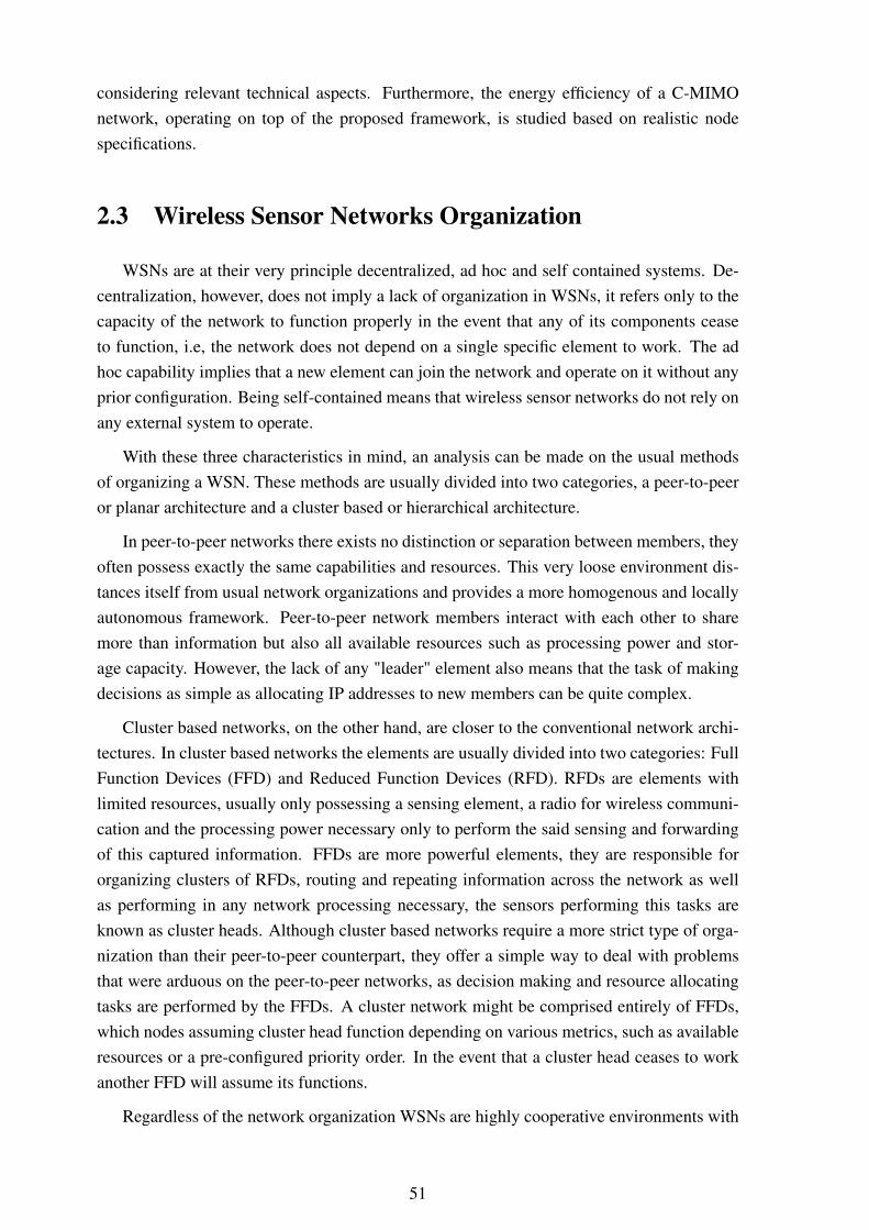
considering relevant technical aspects. Furthermore, the energy efficiency of a C-MIMOnetwork, operating on top of the proposed framework, is studied based on realistic nodespecifications.
2.3 Wireless Sensor Networks Organization
WSNs are at their very principle decentralized, ad hoc and self contained systems. De-centralization, however, does not imply a lack of organization in WSNs, it refers only to thecapacity of the network to function properly in the event that any of its components ceaseto function, i.e, the network does not depend on a single specific element to work. The adhoc capability implies that a new element can join the network and operate on it without anyprior configuration. Being self-contained means that wireless sensor networks do not rely onany external system to operate.
With these three characteristics in mind, an analysis can be made on the usual methodsof organizing a WSN. These methods are usually divided into two categories, a peer-to-peeror planar architecture and a cluster based or hierarchical architecture.
In peer-to-peer networks there exists no distinction or separation between members, theyoften possess exactly the same capabilities and resources. This very loose environment dis-tances itself from usual network organizations and provides a more homogenous and locallyautonomous framework. Peer-to-peer network members interact with each other to sharemore than information but also all available resources such as processing power and stor-age capacity. However, the lack of any "leader" element also means that the task of makingdecisions as simple as allocating IP addresses to new members can be quite complex.
Cluster based networks, on the other hand, are closer to the conventional network archi-tectures. In cluster based networks the elements are usually divided into two categories: FullFunction Devices (FFD) and Reduced Function Devices (RFD). RFDs are elements withlimited resources, usually only possessing a sensing element, a radio for wireless communi-cation and the processing power necessary only to perform the said sensing and forwardingof this captured information. FFDs are more powerful elements, they are responsible fororganizing clusters of RFDs, routing and repeating information across the network as wellas performing in any network processing necessary, the sensors performing this tasks areknown as cluster heads. Although cluster based networks require a more strict type of orga-nization than their peer-to-peer counterpart, they offer a simple way to deal with problemsthat were arduous on the peer-to-peer networks, as decision making and resource allocatingtasks are performed by the FFDs. A cluster network might be comprised entirely of FFDs,which nodes assuming cluster head function depending on various metrics, such as availableresources or a pre-configured priority order. In the event that a cluster head ceases to workanother FFD will assume its functions.
Regardless of the network organization WSNs are highly cooperative environments with
51
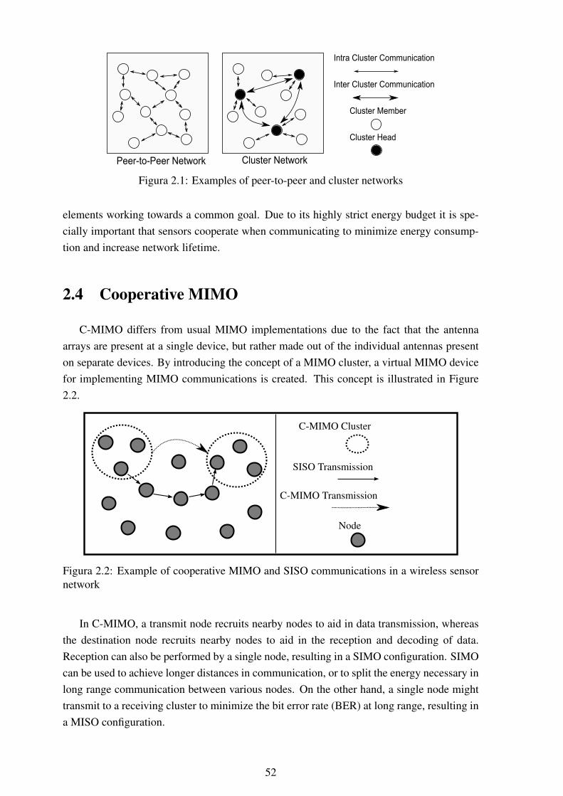
Peer-to-Peer Network Cluster Network
Intra Cluster Communication
Inter Cluster Communication
Cluster Member
Cluster Head
Figura 2.1: Examples of peer-to-peer and cluster networks
elements working towards a common goal. Due to its highly strict energy budget it is spe-cially important that sensors cooperate when communicating to minimize energy consump-tion and increase network lifetime.
2.4 Cooperative MIMO
C-MIMO differs from usual MIMO implementations due to the fact that the antennaarrays are present at a single device, but rather made out of the individual antennas presenton separate devices. By introducing the concept of a MIMO cluster, a virtual MIMO devicefor implementing MIMO communications is created. This concept is illustrated in Figure2.2.
C-MIMO Cluster
SISO Transmission
C-MIMO Transmission
Node
Figura 2.2: Example of cooperative MIMO and SISO communications in a wireless sensornetwork
In C-MIMO, a transmit node recruits nearby nodes to aid in data transmission, whereasthe destination node recruits nearby nodes to aid in the reception and decoding of data.Reception can also be performed by a single node, resulting in a SIMO configuration. SIMOcan be used to achieve longer distances in communication, or to split the energy necessary inlong range communication between various nodes. On the other hand, a single node mighttransmit to a receiving cluster to minimize the bit error rate (BER) at long range, resulting ina MISO configuration.
52
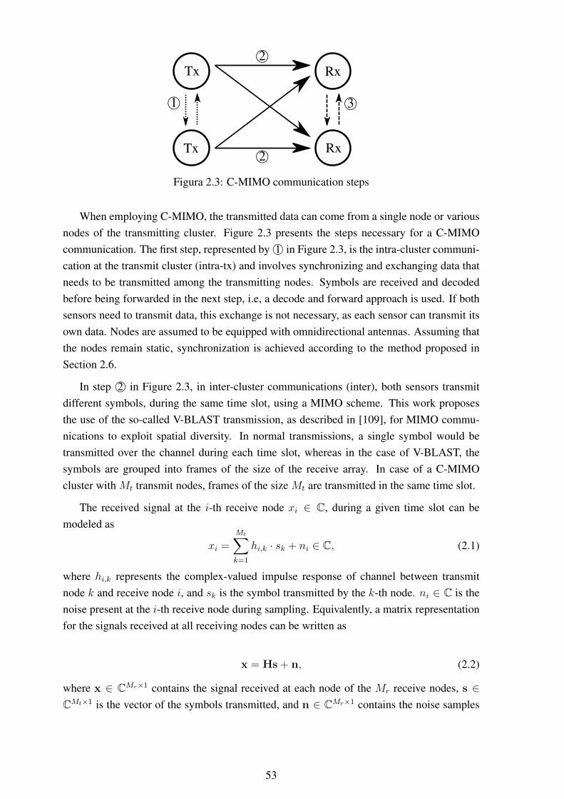
1©
Tx
Tx
Rx
Rx2©
2©
3©
Figura 2.3: C-MIMO communication steps
When employing C-MIMO, the transmitted data can come from a single node or variousnodes of the transmitting cluster. Figure 2.3 presents the steps necessary for a C-MIMOcommunication. The first step, represented by 1© in Figure 2.3, is the intra-cluster communi-cation at the transmit cluster (intra-tx) and involves synchronizing and exchanging data thatneeds to be transmitted among the transmitting nodes. Symbols are received and decodedbefore being forwarded in the next step, i.e, a decode and forward approach is used. If bothsensors need to transmit data, this exchange is not necessary, as each sensor can transmit itsown data. Nodes are assumed to be equipped with omnidirectional antennas. Assuming thatthe nodes remain static, synchronization is achieved according to the method proposed inSection 2.6.
In step 2© in Figure 2.3, in inter-cluster communications (inter), both sensors transmitdifferent symbols, during the same time slot, using a MIMO scheme. This work proposesthe use of the so-called V-BLAST transmission, as described in [109], for MIMO commu-nications to exploit spatial diversity. In normal transmissions, a single symbol would betransmitted over the channel during each time slot, whereas in the case of V-BLAST, thesymbols are grouped into frames of the size of the receive array. In case of a C-MIMOcluster with Mt transmit nodes, frames of the size Mt are transmitted in the same time slot.
The received signal at the i-th receive node xi ∈ C, during a given time slot can bemodeled as
xi =Mt∑k=1
hi,k · sk + ni ∈ C, (2.1)
where hi,k represents the complex-valued impulse response of channel between transmitnode k and receive node i, and sk is the symbol transmitted by the k-th node. ni ∈ C is thenoise present at the i-th receive node during sampling. Equivalently, a matrix representationfor the signals received at all receiving nodes can be written as
x = Hs + n, (2.2)
where x ∈ CMr×1 contains the signal received at each node of the Mr receive nodes, s ∈CMt×1 is the vector of the symbols transmitted, and n ∈ CMr×1 contains the noise samples
53
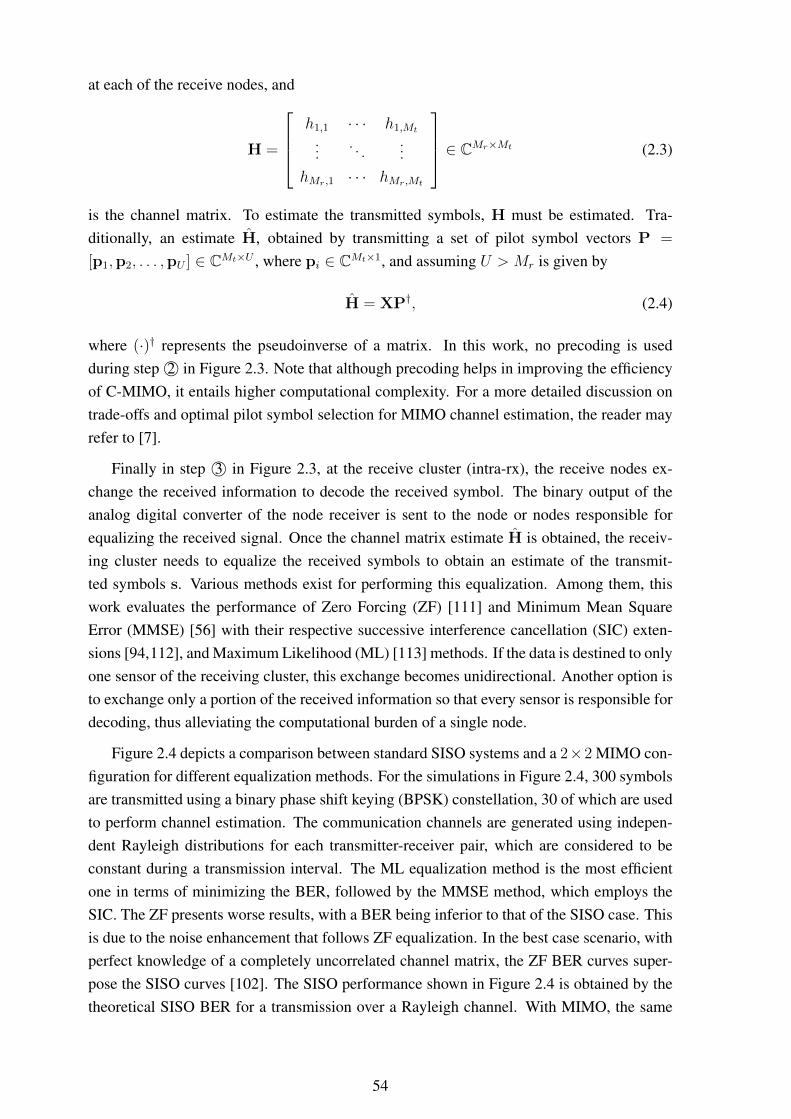
at each of the receive nodes, and
H =
h1,1 · · · h1,Mt
.... . .
...
hMr,1 · · · hMr,Mt
∈ CMr×Mt (2.3)
is the channel matrix. To estimate the transmitted symbols, H must be estimated. Tra-ditionally, an estimate H, obtained by transmitting a set of pilot symbol vectors P =
[p1,p2, . . . ,pU ] ∈ CMt×U , where pi ∈ CMt×1, and assuming U > Mr is given by
H = XP†, (2.4)
where (·)† represents the pseudoinverse of a matrix. In this work, no precoding is usedduring step 2© in Figure 2.3. Note that although precoding helps in improving the efficiencyof C-MIMO, it entails higher computational complexity. For a more detailed discussion ontrade-offs and optimal pilot symbol selection for MIMO channel estimation, the reader mayrefer to [7].
Finally in step 3© in Figure 2.3, at the receive cluster (intra-rx), the receive nodes ex-change the received information to decode the received symbol. The binary output of theanalog digital converter of the node receiver is sent to the node or nodes responsible forequalizing the received signal. Once the channel matrix estimate H is obtained, the receiv-ing cluster needs to equalize the received symbols to obtain an estimate of the transmit-ted symbols s. Various methods exist for performing this equalization. Among them, thiswork evaluates the performance of Zero Forcing (ZF) [111] and Minimum Mean SquareError (MMSE) [56] with their respective successive interference cancellation (SIC) exten-sions [94,112], and Maximum Likelihood (ML) [113] methods. If the data is destined to onlyone sensor of the receiving cluster, this exchange becomes unidirectional. Another option isto exchange only a portion of the received information so that every sensor is responsible fordecoding, thus alleviating the computational burden of a single node.
Figure 2.4 depicts a comparison between standard SISO systems and a 2×2 MIMO con-figuration for different equalization methods. For the simulations in Figure 2.4, 300 symbolsare transmitted using a binary phase shift keying (BPSK) constellation, 30 of which are usedto perform channel estimation. The communication channels are generated using indepen-dent Rayleigh distributions for each transmitter-receiver pair, which are considered to beconstant during a transmission interval. The ML equalization method is the most efficientone in terms of minimizing the BER, followed by the MMSE method, which employs theSIC. The ZF presents worse results, with a BER being inferior to that of the SISO case. Thisis due to the noise enhancement that follows ZF equalization. In the best case scenario, withperfect knowledge of a completely uncorrelated channel matrix, the ZF BER curves super-pose the SISO curves [102]. The SISO performance shown in Figure 2.4 is obtained by thetheoretical SISO BER for a transmission over a Rayleigh channel. With MIMO, the same
54
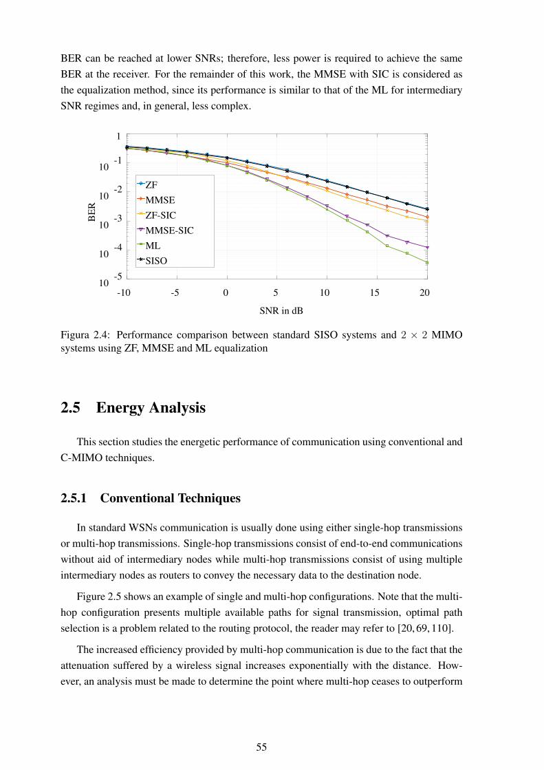
BER can be reached at lower SNRs; therefore, less power is required to achieve the sameBER at the receiver. For the remainder of this work, the MMSE with SIC is considered asthe equalization method, since its performance is similar to that of the ML for intermediarySNR regimes and, in general, less complex.
SNR in dB
-10 -5 0 5 10 15 20
BE
R
10-5
10-4
10-3
10-2
10-1
1
ZF
MMSE
ZF-SIC
MMSE-SIC
ML
SISO
Figura 2.4: Performance comparison between standard SISO systems and 2 × 2 MIMOsystems using ZF, MMSE and ML equalization
2.5 Energy Analysis
This section studies the energetic performance of communication using conventional andC-MIMO techniques.
2.5.1 Conventional Techniques
In standard WSNs communication is usually done using either single-hop transmissionsor multi-hop transmissions. Single-hop transmissions consist of end-to-end communicationswithout aid of intermediary nodes while multi-hop transmissions consist of using multipleintermediary nodes as routers to convey the necessary data to the destination node.
Figure 2.5 shows an example of single and multi-hop configurations. Note that the multi-hop configuration presents multiple available paths for signal transmission, optimal pathselection is a problem related to the routing protocol, the reader may refer to [20, 69, 110].
The increased efficiency provided by multi-hop communication is due to the fact that theattenuation suffered by a wireless signal increases exponentially with the distance. How-ever, an analysis must be made to determine the point where multi-hop ceases to outperform
55

a
b
a
b
Single-hop Communication Multi-hop Communication
a
b
Source Node
Destination Node
Intermediary Node
Figura 2.5: Examples of single-hop and multi-hop communication
single-hop. According to the energy consumption model proposed in [17]
Et = α, (2.5)
Er = β, (2.6)
where Et is the energy necessary for transmitting a single symbol over a certain distance andEr is the energy necessary for receiving and decoding the given symbol. The parameter α isdirectly dependent on the distance between the transmitting and receiving nodes and can bewritten as
α =
a+ b · dγ ; dmax ≥ d > dmin
a+ b · dγmin ; d 6 dmin(2.7)
here dmin defines the maximum distance that can be reached by setting the transmit powerof the transmitting node radio to its minimum configurable value, dmax is the maximumreachable distance by setting the transmit power to its highest configurable value, d is thedistance between the transmitting and receiving nodes and γ is the path loss coefficient. Toevaluate the energy efficiency of both techniques a comparison is made a transmission overdmax using both techniques. Let dmax = k · dmin and the path loss coefficient be equal tothe free space loss coefficient γ = 2 and the power necessary for receiving a signal beingequivalent to the power necessary for minimal transmission β = a. In fact receiving isusually more energy demanding than transmitting at low power as seen on table 2.1.
The total energy consumed in a single-hop transmission can be described by using (2.5)and (2.6) as
Er + Et(dmax) = 2a+ b · d2max = 2a+ b · (k · dmin)2, (2.8)
equivalently, the energy consumed by the multi-hop transmission over k symmetric hops canbe written as
k · Er + k · Et(dmin) = k · a+ k · (a+ b · d2min) = 2 · k · a+ b · k · d2
min. (2.9)
From (2.8) and (2.9) it is possible to derive the condition that makes single-hop more
56

Mode CurrentRx 7.03mA
Tx (-18 dBm) 3.72mATx (-13 dBm) 5.21mATx (-10 dBm) 5.37mATx (-6 dBm) 7.05mATx (-2 dBm) 8.47mATx (0 dBm) 11.57mA
Tx (+3 dBm) 13.77mATx (+4 dBm) 17.37mATx (+5 dBm) 21.48mATx (+10 dBm) 27.01 mA
Tabela 2.1: Energy consumption for the Mica2 platform
energy efficient than multi-hop
k ≤ 2a
b · d2min
. (2.10)
According to [6] [78], a condition necessary for minimizing energy consumption in multi-hop is that the hop distance is the same for all hops. For n intermediary nodes placed betweentwo nodes separated by a distance D the hop distance is
dhop =D
n, (2.11)
replacing dmin with dhop in (2.9) and taking its derivative with respect to n, the number ofhops that minimizes the energy consumption in multi-hop communications can be found
nopt =
√b
2a·D. (2.12)
By replacing n by nopt in (2.11) the optimum hop distance in terms of energy consumptioncan be written as
dchar =
√2a
b, (2.13)
where dchar is known as the characteristic distance. Note that dchar depends only upon thevalues of a and b, thus it is a parameter intrinsic to the sensor in question.
Care must be taken when employing the multi-hop approach to avoid reducing energy ef-ficiency by using an unnecessary number of hops. When adequately employed the multi-hopapproach can lead to significant energy saving in WSNs. However, multi-hopping suffersfrom some serious disadvantages. Data forwarding is usually done on a best effort deliv-ery basis. That means that the transmitting node has no guarantee of the transmitted datareaching its destination, or that it will be delivered within a given time frame. Multi-hopnetworking can lead to data congestion on nodes that are located between node clusters thatgenerate heavy traffic. This heavy traffic will also result in a high drain of energy resources
57

the in the nodes responsible for forwarding the data. This will result in a high delivery delayand will eventually lead to depletion of energy in these midway nodes, resulting in a dis-connected network. Data relaying is usually done in a decode and forward fashion, this canresult in a high delay even when there is no network congestion present.
Single-hop transmissions are not affected by network congestion as they are end-to-endcommunications, but they require a very high signal power when employed over large dis-tances. If a single sensor is responsible for producing a large amount of data that needsto be transmitted over a large distance, this will lead to a very fast depletion of its energyresources. This uneven depletion is highly prejudicial to WSN operation, since replacingindividual nodes might be as costly as replacing the entire network. Furthermore, single-hoptransmissions might be unattainable over large distances due to the limited power at whichsensor radios usually operate.
2.5.2 Cooperative MIMO
By introducing the C-MIMO approach, the drawbacks of the multi-hop approach, suchas larger delay and possible uneven energy consumption, can be avoided while still achievingenergy efficient communications. With the fundamentals of C-MIMO reviewed in Section2.4, a reliable, low BER and energy efficient communication can be implemented by takingadvantage of the cooperative nature of WSNs.
With the steps of Figure 2.3 in mind, it is possible to derive an analytical expression forthe energy consumption of C-MIMO. Defining Eintra as the energy necessary to transmit anentire data packet to another sensor located within the C-MIMO cluster frontier, shown as1© and 3© in Figure 2.3, the energy spent on spreading the packet for transmission and for
consolidating it for equalization and decoding is given by
Etxintratx=Mt − 1
Mt
Eintra, (2.14)
Etxintrarx=Mr − 1
Mr
Eintra, (2.15)
respectively. For anMt×Mr C-MIMO transmission, a central node that spreads its packet toneighboring nodes needs to performMt−1 transmissions with a cost of Eintra
Mt, as the packet is
split into Mt smaller packets for C-MIMO transmission. The same applies to consolidatingthe packet on the receiving C-MIMO cluster, whereMr−1 transmissions with a cost of Eintra
Mr,
are sent to a central node for equalization and decoding.
Dissemination and consolidation of packets on the C-MIMO clusters also consume sig-nificant energy on the radios listening to the transmissions. Therefore,Mt−1 receptions witha cost of Erx
Mt, where Erx is the energy cost for receiving an entire data packet, are necessary
at the transmitting cluster. At the receiving cluster, Mr − 1 receptions with a cost of ErxMr
are
58

necessary when the received symbols are transmitted to the central node for decoding. Thus,the energy spent with receptions at the transmitting and receiver clusters is given by
Erxintratx=
(Mt − 1)
Mt
Erx, (2.16)
Erxintrarx=
(Mr − 1)
Mr
Erx, (2.17)
respectively. Additionally, as the packet is transmitting over long distances using C-MIMO,the Mr receiving nodes must listen. Therefore, another Mr receptions with Erx
Mrcost are
necessary.
Finally, Etxinteris the energy spent on transmitting a data packet, using higher power
for the long distance transmission step 2© on Figure 2.3. Mt nodes transmit 1Mt
of the datapacket.
The total cost for transmitting a packet, using cooperative MIMO, is then given by
EC-MIMO = Etxinter+ Etxintratx
+ Etxintrarx
+Erxintratx+ Erxintrarx
+ Erx. (2.18)
C-MIMO is capable of reaching large distances without demanding much power from asingle node. In addition, since multiple copies of the same signal are received, the BER isconsiderably smaller at the same SNR. This makes the C-MIMO capable of reaching longdistances, using much less power than SISO configurations do. C-MIMO configurationscan lead to even lower BER ratios, which allow even less power to be used for long rangetransmissions.
Next, assuming a multihop communication where the nodes involved are uniformlyspaced and the energy necessary to transmit a data packet to the next node is equivalentto the energy necessary to transmit inside a C-MIMO cluster, Eintra, the energy used for amultihop transmission is given by
Emhop = k (Eintra + Erx) , (2.19)
where k is the number of hops necessary to reach the destination node. From (2.18) and(2.19), the condition under which C-MIMO becomes more efficient than multihop, i.e.EC−MIMO < Emhop, is
Einter <
(k −
(Mt − 1
Mt
+Mr − 1
Mr
))Eintra
+
(k −
(Mt − 1
Mt
+Mr − 1
Mr
+ 1
))Erx. (2.20)
59
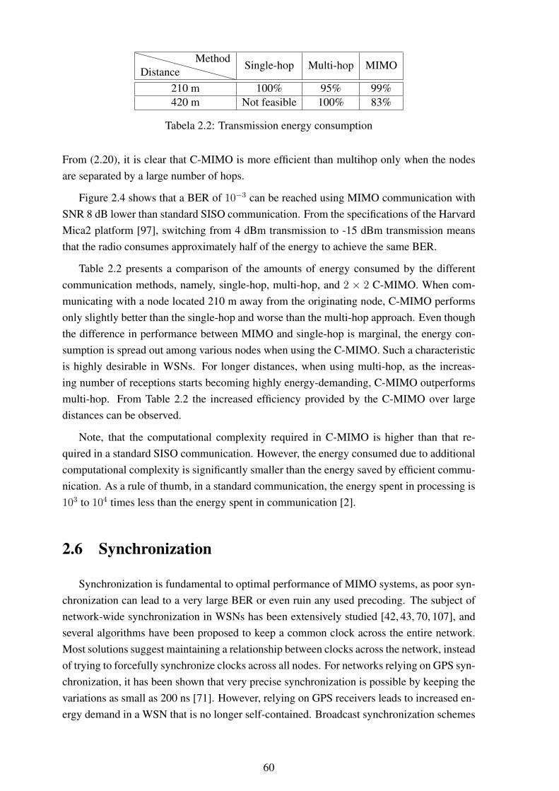
DistanceMethod
Single-hop Multi-hop MIMO
210 m 100% 95% 99%420 m Not feasible 100% 83%
Tabela 2.2: Transmission energy consumption
From (2.20), it is clear that C-MIMO is more efficient than multihop only when the nodesare separated by a large number of hops.
Figure 2.4 shows that a BER of 10−3 can be reached using MIMO communication withSNR 8 dB lower than standard SISO communication. From the specifications of the HarvardMica2 platform [97], switching from 4 dBm transmission to -15 dBm transmission meansthat the radio consumes approximately half of the energy to achieve the same BER.
Table 2.2 presents a comparison of the amounts of energy consumed by the differentcommunication methods, namely, single-hop, multi-hop, and 2 × 2 C-MIMO. When com-municating with a node located 210 m away from the originating node, C-MIMO performsonly slightly better than the single-hop and worse than the multi-hop approach. Even thoughthe difference in performance between MIMO and single-hop is marginal, the energy con-sumption is spread out among various nodes when using the C-MIMO. Such a characteristicis highly desirable in WSNs. For longer distances, when using multi-hop, as the increas-ing number of receptions starts becoming highly energy-demanding, C-MIMO outperformsmulti-hop. From Table 2.2 the increased efficiency provided by the C-MIMO over largedistances can be observed.
Note, that the computational complexity required in C-MIMO is higher than that re-quired in a standard SISO communication. However, the energy consumed due to additionalcomputational complexity is significantly smaller than the energy saved by efficient commu-nication. As a rule of thumb, in a standard communication, the energy spent in processing is103 to 104 times less than the energy spent in communication [2].
2.6 Synchronization
Synchronization is fundamental to optimal performance of MIMO systems, as poor syn-chronization can lead to a very large BER or even ruin any used precoding. The subject ofnetwork-wide synchronization in WSNs has been extensively studied [42, 43, 70, 107], andseveral algorithms have been proposed to keep a common clock across the entire network.Most solutions suggest maintaining a relationship between clocks across the network, insteadof trying to forcefully synchronize clocks across all nodes. For networks relying on GPS syn-chronization, it has been shown that very precise synchronization is possible by keeping thevariations as small as 200 ns [71]. However, relying on GPS receivers leads to increased en-ergy demand in a WSN that is no longer self-contained. Broadcast synchronization schemes
60

capable of achieving 1 µs of accuracy have been proposed in [36].
Subsection 2.6.1 presents an analysis of the effects of synchronization errors on WSNsoperating with C-MIMO and V-BLAST. To mitigate such effects, two synchronizationschemes are proposed for WSNs operating with C-MIMO. A method for coarse synchro-nization is presented in Subsection 2.6.2. Since WSNs can also be composed of nodeswith limited processing capabilities, a method for accurate synchronization that requires lowcomputational effort is proposed. Similarly, for networks with higher processing power, amethod that provides highly accurate synchronization is proposed. These methods are de-tailed in Subsection 2.6.3. Finally, Subsection 2.6.4 presents an analysis of the propagationof synchronization errors in WSNs, besides a study on how to choose the appropriate symbolduration and re-synchronization interval of the network to allow the use of C-MIMO.
2.6.1 Effects of Synchronization Error on Cooperative MIMO
For networks operating at 256 ksps rate, the resulting symbol duration is approximately4 µs. In this case, a synchronization error of 1 µs represents 25 % of symbol duration. Inpractice, synchronization errors result in a lower SNR, implying a lower BER performancefor a fixed noise power at the receiver. Figures 2.6, 2.7, and 2.8 compare the performances ofthe equalization methods discussed in this work in the presence of a synchronization errors,expressed as fractions of the symbol period Ts, for MIMO systems with different numbersof elements. The results show that, for smaller configurations, errors as small as 0.2Ts canhave a large impact on the BER performance of MIMO communications, specially for SICvariants due to the error propagation problem caused when a symbol is decoded incorrectly.While larger configurations are shown to be more robust to synchronization errors, achievingsuch configuration in a C-MIMO scheme may not be always possible, since it depends, forinstance, on the node density of the network or the overall processing power of the noderesponsible for equalization and decoding. Therefore, another method for synchronizingtransmitting nodes and receiving nodes is necessary to take full advantage of MIMO com-munications in WSNs.
2.6.2 Proposed Coarse Synchronization Scheme
To achieve a degree of synchronization compatible with the operation of C-MIMO, thiswork proposes scheduling a tonal transmission between a pair of nodes or tonal broadcastto a group of nodes. The sampling on the receiving nodes starts at the scheduled time, andthe clock error can be compensated by comparing the received tonal wave with a referencewave kept internally. The comparison can be done using ML or discrete Fourier transformbased methods. However, owning to the periodic nature of the tonal waves, an element ofambiguity creeps in for delays higher than a wave period. Therefore, the receive node needsto be synchronized first with an accuracy of a period of the transmitted tonal wave.
61
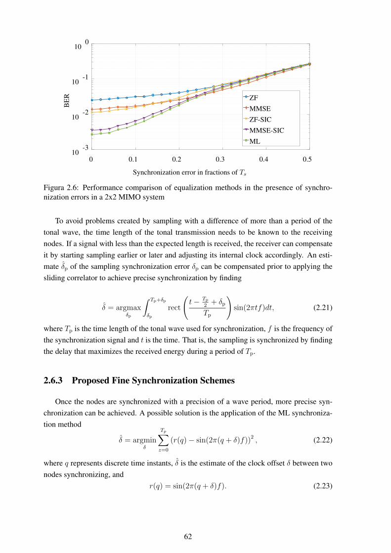
Synchronization error in fractions of Ts
0 0.1 0.2 0.3 0.4 0.5
BE
R
10-3
10-2
10-1
100
ZF
MMSE
ZF-SIC
MMSE-SIC
ML
Figura 2.6: Performance comparison of equalization methods in the presence of synchro-nization errors in a 2x2 MIMO system
To avoid problems created by sampling with a difference of more than a period of thetonal wave, the time length of the tonal transmission needs to be known to the receivingnodes. If a signal with less than the expected length is received, the receiver can compensateit by starting sampling earlier or later and adjusting its internal clock accordingly. An esti-mate δp of the sampling synchronization error δp can be compensated prior to applying thesliding correlator to achieve precise synchronization by finding
δ = argmaxδp
∫ Tp+δp
δp
rect
(t− Tp
2+ δp
Tp
)sin(2πtf)dt, (2.21)
where Tp is the time length of the tonal wave used for synchronization, f is the frequency ofthe synchronization signal and t is the time. That is, the sampling is synchronized by findingthe delay that maximizes the received energy during a period of Tp.
2.6.3 Proposed Fine Synchronization Schemes
Once the nodes are synchronized with a precision of a wave period, more precise syn-chronization can be achieved. A possible solution is the application of the ML synchroniza-tion method
δ = argminδ
Tp∑z=0
(r(q)− sin(2π(q + δ)f))2 , (2.22)
where q represents discrete time instants, δ is the estimate of the clock offset δ between twonodes synchronizing, and
r(q) = sin(2π(q + δ)f). (2.23)
62
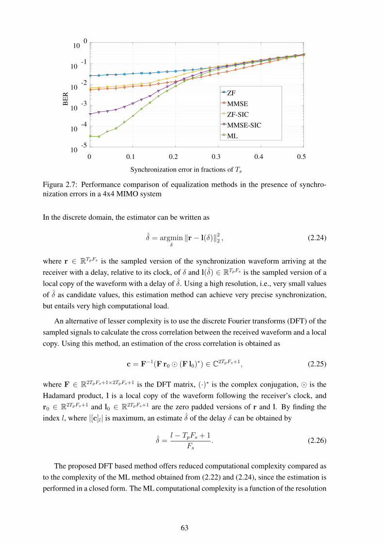
Synchronization error in fractions of Ts
0 0.1 0.2 0.3 0.4 0.5
BE
R
10-5
10-4
10-3
10-2
10-1
100
ZF
MMSE
ZF-SIC
MMSE-SIC
ML
Figura 2.7: Performance comparison of equalization methods in the presence of synchro-nization errors in a 4x4 MIMO system
In the discrete domain, the estimator can be written as
δ = argminδ‖r− l(δ)‖2
2 , (2.24)
where r ∈ RTpFs is the sampled version of the synchronization waveform arriving at thereceiver with a delay, relative to its clock, of δ and l(δ) ∈ RTpFs is the sampled version of alocal copy of the waveform with a delay of δ. Using a high resolution, i.e., very small valuesof δ as candidate values, this estimation method can achieve very precise synchronization,but entails very high computational load.
An alternative of lesser complexity is to use the discrete Fourier transforms (DFT) of thesampled signals to calculate the cross correlation between the received waveform and a localcopy. Using this method, an estimation of the cross correlation is obtained as
c = F−1(F r0 � (F l0)∗) ∈ C2TpFs+1, (2.25)
where F ∈ R2TpFs+1×2TpFs+1 is the DFT matrix, (·)∗ is the complex conjugation, � is theHadamard product, l is a local copy of the waveform following the receiver’s clock, andr0 ∈ R2TpFs+1 and l0 ∈ R2TpFs+1 are the zero padded versions of r and l. By finding theindex l, where |[c]l| is maximum, an estimate δ of the delay δ can be obtained by
δ =l − TpFs + 1
Fs. (2.26)
The proposed DFT based method offers reduced computational complexity compared asto the complexity of the ML method obtained from (2.22) and (2.24), since the estimation isperformed in a closed form. The ML computational complexity is a function of the resolution
63
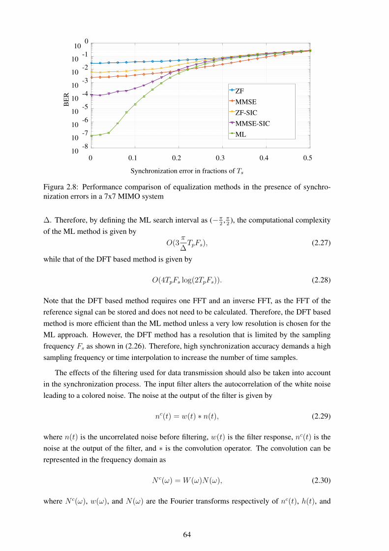
Synchronization error in fractions of Ts
0 0.1 0.2 0.3 0.4 0.5
BE
R
10-8
10-7
10-6
10-5
10-4
10-3
10-2
10-1
100
ZF
MMSE
ZF-SIC
MMSE-SIC
ML
Figura 2.8: Performance comparison of equalization methods in the presence of synchro-nization errors in a 7x7 MIMO system
∆. Therefore, by defining the ML search interval as (−π2,π2), the computational complexity
of the ML method is given byO(3
π
∆TpFs), (2.27)
while that of the DFT based method is given by
O(4TpFs log(2TpFs)). (2.28)
Note that the DFT based method requires one FFT and an inverse FFT, as the FFT of thereference signal can be stored and does not need to be calculated. Therefore, the DFT basedmethod is more efficient than the ML method unless a very low resolution is chosen for theML approach. However, the DFT method has a resolution that is limited by the samplingfrequency Fs as shown in (2.26). Therefore, high synchronization accuracy demands a highsampling frequency or time interpolation to increase the number of time samples.
The effects of the filtering used for data transmission should also be taken into accountin the synchronization process. The input filter alters the autocorrelation of the white noiseleading to a colored noise. The noise at the output of the filter is given by
nc(t) = w(t) ∗ n(t), (2.29)
where n(t) is the uncorrelated noise before filtering, w(t) is the filter response, nc(t) is thenoise at the output of the filter, and ∗ is the convolution operator. The convolution can berepresented in the frequency domain as
N c(ω) = W (ω)N(ω), (2.30)
where N c(ω), w(ω), and N(ω) are the Fourier transforms respectively of nc(t), h(t), and
64
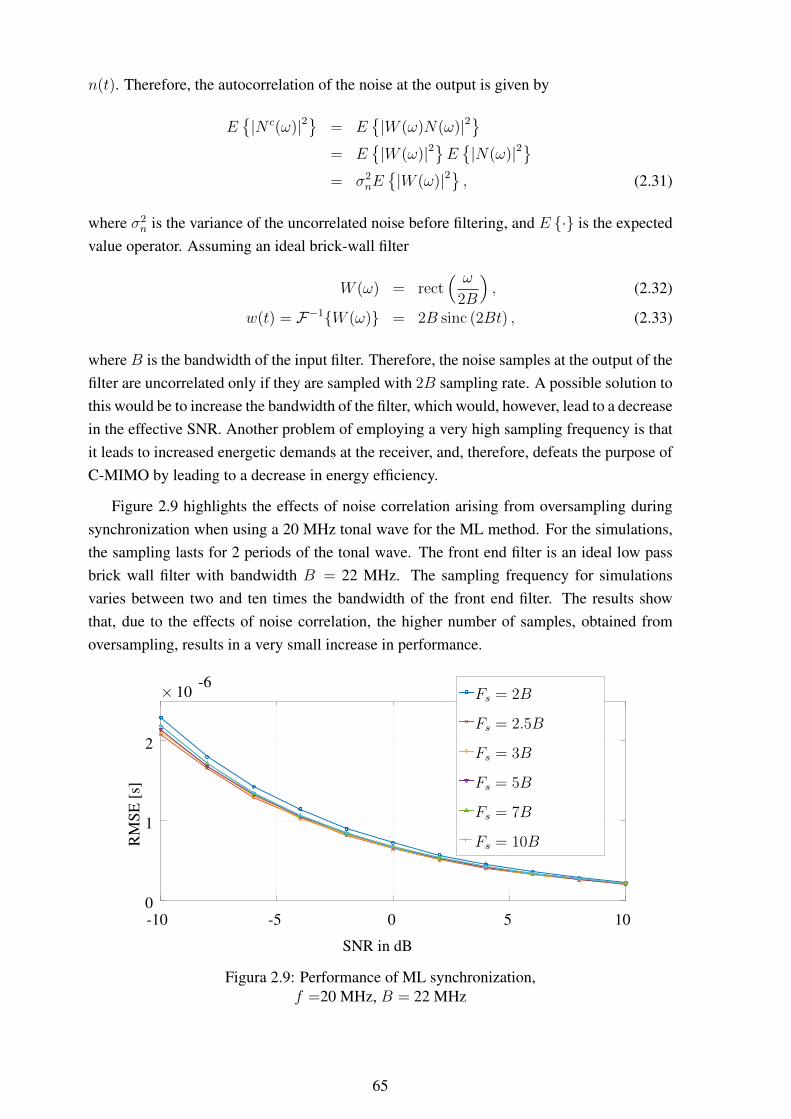
n(t). Therefore, the autocorrelation of the noise at the output is given by
E{|N c(ω)|2
}= E
{|W (ω)N(ω)|2
}= E
{|W (ω)|2
}E{|N(ω)|2
}= σ2
nE{|W (ω)|2
}, (2.31)
where σ2n is the variance of the uncorrelated noise before filtering, and E {·} is the expected
value operator. Assuming an ideal brick-wall filter
W (ω) = rect( ω
2B
), (2.32)
w(t) = F−1{W (ω)} = 2B sinc (2Bt) , (2.33)
where B is the bandwidth of the input filter. Therefore, the noise samples at the output of thefilter are uncorrelated only if they are sampled with 2B sampling rate. A possible solution tothis would be to increase the bandwidth of the filter, which would, however, lead to a decreasein the effective SNR. Another problem of employing a very high sampling frequency is thatit leads to increased energetic demands at the receiver, and, therefore, defeats the purpose ofC-MIMO by leading to a decrease in energy efficiency.
Figure 2.9 highlights the effects of noise correlation arising from oversampling duringsynchronization when using a 20 MHz tonal wave for the ML method. For the simulations,the sampling lasts for 2 periods of the tonal wave. The front end filter is an ideal low passbrick wall filter with bandwidth B = 22 MHz. The sampling frequency for simulationsvaries between two and ten times the bandwidth of the front end filter. The results showthat, due to the effects of noise correlation, the higher number of samples, obtained fromoversampling, results in a very small increase in performance.
SNR in dB
-10 -5 0 5 10
RM
SE[s
]
× 10-6
0
1
2
Fs = 2B
Fs = 2.5B
Fs = 3B
Fs = 5B
Fs = 7B
Fs = 10B
Figura 2.9: Performance of ML synchronization,f =20 MHz, B = 22 MHz
65
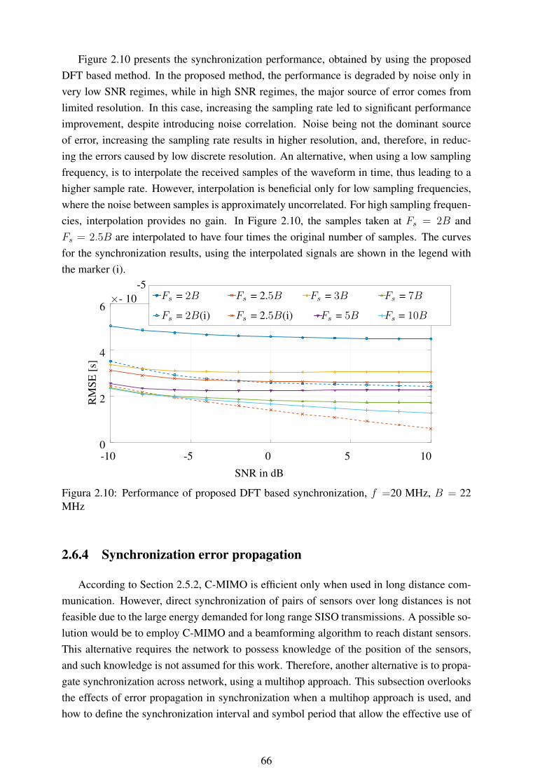
Figure 2.10 presents the synchronization performance, obtained by using the proposedDFT based method. In the proposed method, the performance is degraded by noise only invery low SNR regimes, while in high SNR regimes, the major source of error comes fromlimited resolution. In this case, increasing the sampling rate led to significant performanceimprovement, despite introducing noise correlation. Noise being not the dominant sourceof error, increasing the sampling rate results in higher resolution, and, therefore, in reduc-ing the errors caused by low discrete resolution. An alternative, when using a low samplingfrequency, is to interpolate the received samples of the waveform in time, thus leading to ahigher sample rate. However, interpolation is beneficial only for low sampling frequencies,where the noise between samples is approximately uncorrelated. For high sampling frequen-cies, interpolation provides no gain. In Figure 2.10, the samples taken at Fs = 2B andFs = 2.5B are interpolated to have four times the original number of samples. The curvesfor the synchronization results, using the interpolated signals are shown in the legend withthe marker (i).
SNR in dB
-10 -5 0 5 10
RM
SE[s
]
×- 10-5
0
2
4
6Fs = 2B
Fs = 2B(i)
Fs = 2.5B
Fs = 2.5B(i)
Fs = 3B
Fs = 5B
Fs = 7B
Fs = 10B
Figura 2.10: Performance of proposed DFT based synchronization, f =20 MHz, B = 22MHz
2.6.4 Synchronization error propagation
According to Section 2.5.2, C-MIMO is efficient only when used in long distance com-munication. However, direct synchronization of pairs of sensors over long distances is notfeasible due to the large energy demanded for long range SISO transmissions. A possible so-lution would be to employ C-MIMO and a beamforming algorithm to reach distant sensors.This alternative requires the network to possess knowledge of the position of the sensors,and such knowledge is not assumed for this work. Therefore, another alternative is to propa-gate synchronization across network, using a multihop approach. This subsection overlooksthe effects of error propagation in synchronization when a multihop approach is used, andhow to define the synchronization interval and symbol period that allow the effective use of
66
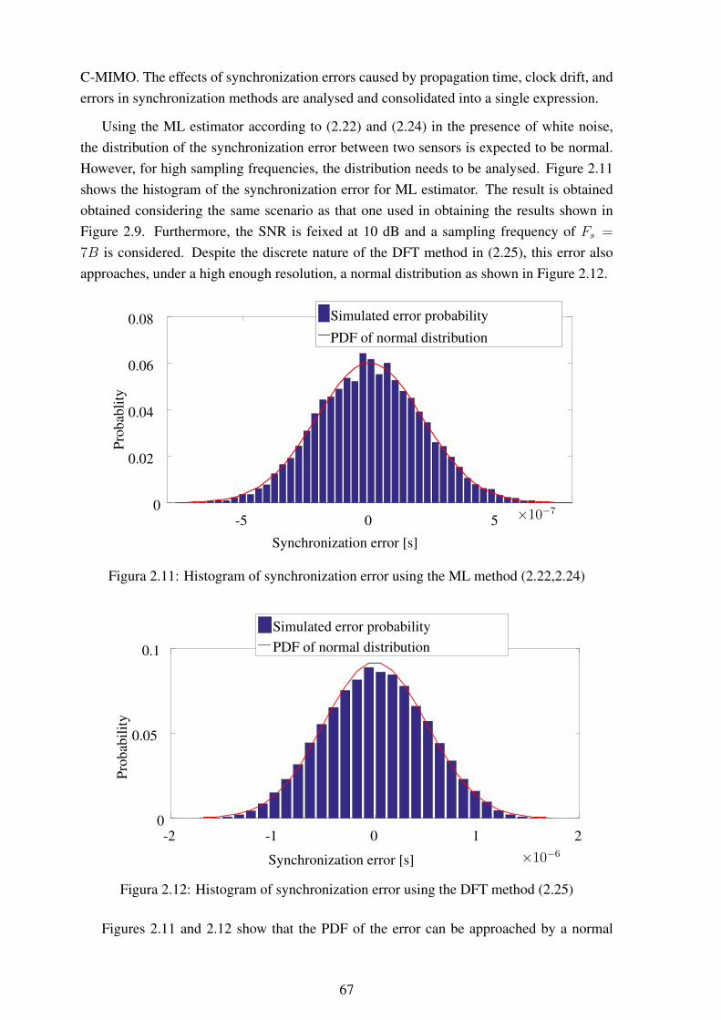
C-MIMO. The effects of synchronization errors caused by propagation time, clock drift, anderrors in synchronization methods are analysed and consolidated into a single expression.
Using the ML estimator according to (2.22) and (2.24) in the presence of white noise,the distribution of the synchronization error between two sensors is expected to be normal.However, for high sampling frequencies, the distribution needs to be analysed. Figure 2.11shows the histogram of the synchronization error for ML estimator. The result is obtainedobtained considering the same scenario as that one used in obtaining the results shown inFigure 2.9. Furthermore, the SNR is feixed at 10 dB and a sampling frequency of Fs =
7B is considered. Despite the discrete nature of the DFT method in (2.25), this error alsoapproaches, under a high enough resolution, a normal distribution as shown in Figure 2.12.
Synchronization error [s]
×10−7-5 0 5
Prob
ablit
y
0
0.02
0.04
0.06
0.08 Simulated error probability
PDF of normal distribution
Figura 2.11: Histogram of synchronization error using the ML method (2.22,2.24)
Synchronization error [s] ×10−6
-2 -1 0 1 2
Prob
abili
ty
0
0.05
0.1
Simulated error probabilityPDF of normal distribution
Figura 2.12: Histogram of synchronization error using the DFT method (2.25)
Figures 2.11 and 2.12 show that the PDF of the error can be approached by a normal
67
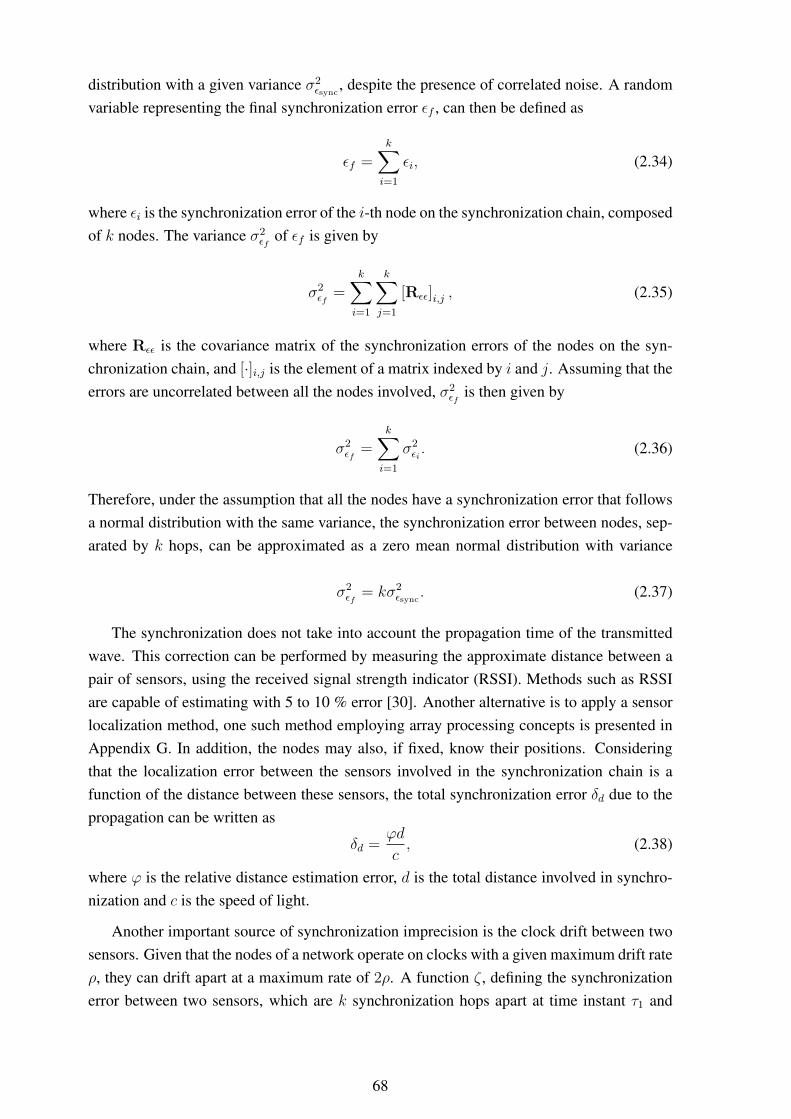
distribution with a given variance σ2εsync
, despite the presence of correlated noise. A randomvariable representing the final synchronization error εf , can then be defined as
εf =k∑i=1
εi, (2.34)
where εi is the synchronization error of the i-th node on the synchronization chain, composedof k nodes. The variance σ2
εfof εf is given by
σ2εf
=k∑i=1
k∑j=1
[Rεε]i,j , (2.35)
where Rεε is the covariance matrix of the synchronization errors of the nodes on the syn-chronization chain, and [·]i,j is the element of a matrix indexed by i and j. Assuming that theerrors are uncorrelated between all the nodes involved, σ2
εfis then given by
σ2εf
=k∑i=1
σ2εi. (2.36)
Therefore, under the assumption that all the nodes have a synchronization error that followsa normal distribution with the same variance, the synchronization error between nodes, sep-arated by k hops, can be approximated as a zero mean normal distribution with variance
σ2εf
= kσ2εsync
. (2.37)
The synchronization does not take into account the propagation time of the transmittedwave. This correction can be performed by measuring the approximate distance between apair of sensors, using the received signal strength indicator (RSSI). Methods such as RSSIare capable of estimating with 5 to 10 % error [30]. Another alternative is to apply a sensorlocalization method, one such method employing array processing concepts is presented inAppendix G. In addition, the nodes may also, if fixed, know their positions. Consideringthat the localization error between the sensors involved in the synchronization chain is afunction of the distance between these sensors, the total synchronization error δd due to thepropagation can be written as
δd =ϕd
c, (2.38)
where ϕ is the relative distance estimation error, d is the total distance involved in synchro-nization and c is the speed of light.
Another important source of synchronization imprecision is the clock drift between twosensors. Given that the nodes of a network operate on clocks with a given maximum drift rateρ, they can drift apart at a maximum rate of 2ρ. A function ζ , defining the synchronizationerror between two sensors, which are k synchronization hops apart at time instant τ1 and
68
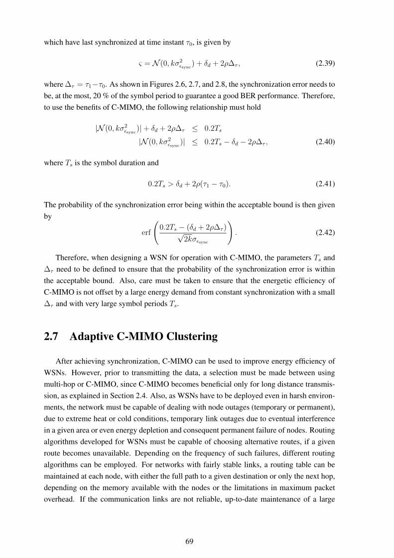
which have last synchronized at time instant τ0, is given by
ς = N (0, kσ2εsync
) + δd + 2ρ∆τ , (2.39)
where ∆τ = τ1−τ0. As shown in Figures 2.6, 2.7, and 2.8, the synchronization error needs tobe, at the most, 20 % of the symbol period to guarantee a good BER performance. Therefore,to use the benefits of C-MIMO, the following relationship must hold
|N (0, kσ2εsync
)|+ δd + 2ρ∆τ ≤ 0.2Ts
|N (0, kσ2εsync
)| ≤ 0.2Ts − δd − 2ρ∆τ , (2.40)
where Ts is the symbol duration and
0.2Ts > δd + 2ρ(τ1 − τ0). (2.41)
The probability of the synchronization error being within the acceptable bound is then givenby
erf
(0.2Ts − (δd + 2ρ∆τ )√
2kσεsync
). (2.42)
Therefore, when designing a WSN for operation with C-MIMO, the parameters Ts and∆τ need to be defined to ensure that the probability of the synchronization error is withinthe acceptable bound. Also, care must be taken to ensure that the energetic efficiency ofC-MIMO is not offset by a large energy demand from constant synchronization with a small∆τ and with very large symbol periods Ts.
2.7 Adaptive C-MIMO Clustering
After achieving synchronization, C-MIMO can be used to improve energy efficiency ofWSNs. However, prior to transmitting the data, a selection must be made between usingmulti-hop or C-MIMO, since C-MIMO becomes beneficial only for long distance transmis-sion, as explained in Section 2.4. Also, as WSNs have to be deployed even in harsh environ-ments, the network must be capable of dealing with node outages (temporary or permanent),due to extreme heat or cold conditions, temporary link outages due to eventual interferencein a given area or even energy depletion and consequent permanent failure of nodes. Routingalgorithms developed for WSNs must be capable of choosing alternative routes, if a givenroute becomes unavailable. Depending on the frequency of such failures, different routingalgorithms can be employed. For networks with fairly stable links, a routing table can bemaintained at each node, with either the full path to a given destination or only the next hop,depending on the memory available with the nodes or the limitations in maximum packetoverhead. If the communication links are not reliable, up-to-date maintenance of a large
69

routing table in every node of the network might not be possible. In such cases, routing algo-rithms such as Ad hoc On-Demand Distance Vector (AODV), are generally used, in whichpaths are discovered only on demand, thus avoiding the need for maintaining routing tableson the nodes.
This Section is divided into two subsections. Subsection 2.7.1 details the proposedmethod for adaptively forming C-MIMO clusters according to the energy efficiency of dif-ferent cluster sizes and according to the impact of different clusters sizes on the distributionof available energy over neighboring nodes. Subsection 2.7.2 presents the numerical simula-tions for the proposed method, highlighting positive effects on network lifetime and energydistribution.
2.7.1 Adaptive C-MIMO clustering
Possible C-MIMO formations for a given node can be represented as new edges withdifferent values on a graph. Therefore, the existence of C-MIMO can be transparent to thechosen routing algorithm. Moreover, since C-MIMO can be used with different cluster sizes,it is important to choose the best possible cluster size for reaching a given node in the networkand representing it on the routing graph as a vertex with the lowest possible cost. Anotherimportant characteristic of C-MIMO is its ability to distribute energy consumption amongvarious nodes, and, depending on the number of neighbors of a given node, the node maychoose the neighbors that cooperate on a C-MIMO transmission to maximize the life time ofthe network. .
Choosing between C-MIMO, multi-hop, and single-hop is not enough. Since C-MIMOcan be used with different cluster sizes, it is important to choose the best possible cluster sizefor reaching a given node in the network, representing it on the routing graph as a vertex withthe lowest possible cost. However, minimizing energy consumption is, by itself, not enoughto maximize the lifetime of a WSN. If energy consumption is low but the energy distributionis uneven, some nodes will fail before others. This distribution can be area dependent, forinstance, regions with a high traffic of information will tend to be depleted ahead of the restof the network. Node failures in such areas might lead to a disconnected network, reducingthe effective lifetime of the network. Generally, it is desirable that the nodes in a WSN havetheir energy reserves evenly depleted, so that the network can stay fully connected as longas it is operational. Therefore, by being aware of the energy reserves of its neighbours, anode can, when using C-MIMO, choose the configuration and neighbours that minimize thedifference between the energy reserves of its neighbours.
This work proposes calculating the cost of a transmission as a function of transmissionpower, cluster size and effects on the energy reserves of neighbours. The metric shown in(2.43) is used to define the cost of a transmission between a pair of nodes indexed by n =
1, . . . , L and m = 1, . . . , L. In this expression L is the number of nodes that compose thenetwork, w = 1, . . . ,W indexes the possible sizes for the C-MIMO clusters up to the limit
70
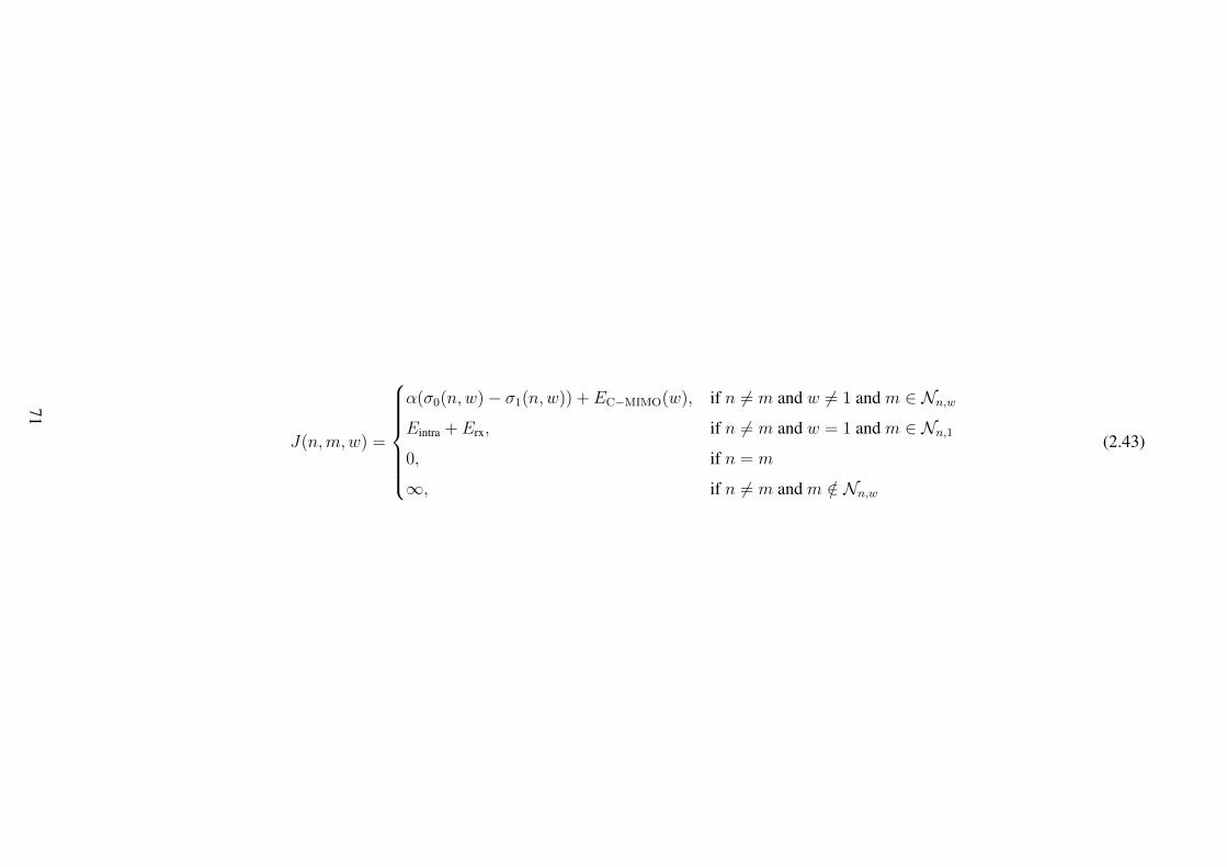
J(n,m,w) =
α(σ0(n,w)− σ1(n,w)) + EC−MIMO(w), if n 6= m and w 6= 1 and m ∈ Nn,wEintra + Erx, if n 6= m and w = 1 and m ∈ Nn,10, if n = m
∞, if n 6= m and m /∈ Nn,w
(2.43)
71

W , EC−MIMO(w) is the energy cost for a C-MIMO transmission using clusters composed ofw elements, σ0(n,m,w) and σ1(n,m,w) are the standard deviations of the energy availablein the node’s neighbours before and after the possible C-MIMO transmission. Nn,w is the setof nodes that can be reached by node n with a C-MIMO cluster size w. For a fixed clustersize, the nodes n and m always choose the neighbours with the highest amount of energy tomaximize the network lifetime. However, it is possible that some formations, even if the totalenergy cost is lower, cause the variance of the energy available on the neighbours to increasetoo much. This means that the distribution of the available energy between the nodes isless uniform leading to some nodes running out of energy before others, and resulting in adisconnected network. Finally, α is a weighting factor that dictates the importance of keepinga uniform energy reserve versus the importance of minimizing overall communication energyconsumption. If the transmit node n has knowledge about the state of the energy reserves ofthe receive cluster it may also take into account its changes on the calculation of the cost.
Each node n stores the cost relative to reaching a given neighbor in a cost matrix
[Rn]m,w = J(n,m,w) ∈ R. (2.44)
A graph used for routing can be set up by grouping all of the cost matrices from the nodesthat form the network into a tensor structure
R = [R1|R2| . . . |RL] ∈ RL×L×W , (2.45)
where | denotes a stacking operation onto the first dimension. However, constructing a graphbased on this structure will result in vertices that are connected by multiple edges, sincenodes can communicate using different C-MIMO cluster sizes. To avoid this problem, someedges must be filtered from the graph. This decision is simple, and can be based solely onthe cost of the edges, leaving only the edges with the smallest cost between two vertices.Therefore, the decision on what cluster size sn,m to use to communicate between a pair ofnodes is given by
sn,m = argminw
[R]n,m,w ∈ N+. (2.46)
Algorithm 1 presents the proposed solution for choosing the optimal cluster formationfor reaching a given node. A list of neighbors is present at each node and associated to it.Moreover, the list includes information about the number of nodes involved in the C-MIMOclusters for reaching the intended destination.
The cost can be a function of variables such as transmission power, cluster size andeffects on the energy reserves of neighbours. This work uses the following metric to definethe cost of C-MIMO transmission
J(σ20, σ
21, EC−MIMO) = α(σ2
0 − σ21) + EC−MIMO, (2.47)
72

Algorithm 1 Lower Cost Hop1: load neighborList2: if routePacketReceived then3: nodes← routePacket.getOriginNodes()4: size← routePacket.clusterSize()5: cost← calculateCost(routePacket)6: for node : nodes do7: if neighborList.contains(node) then8: if node.cost() > cost then9: neighborList.remove(node)
10: neighborList.add(node, cost, size)11: end if12: else13: neighborList.add(node, cost, size)14: end if15: end for16: end if
where Ec-mimo is the energy cost for a C-MIMO transmission as computed in (2.18), σ2o and
σ21 are the variances of the energy available in the neighbouring nodes, before and after
the possible C-MIMO transmission. For a fixed cluster size, the node always chooses theneighbours with the highest amount of energy to maximize the network lifetime. However, itis possible that some formations, even if the total energy cost is low, significantly increase thedifference between the energy levels of the neighbours. Thus, the distribution of the availableenergy between the nodes becomes less uniform. This will lead to some nodes running outof energy before others do, which may ultimately result in a disconnected network. Finally,α is the weighting factor that dictates need for maintaining a uniform energy reserve versusthe need for minimizing overall communication energy consumption. If the transmit nodehas knowledge about the state of the energy reserves of the receive cluster it may also takeinto account its changes on the calculation of the cost.
Other parameters such as delay, packet loss or available bandwidth may also be includedin the metrics of cost function. If one of the nodes transmitting the packet is not entered inthe list, this entry is added on the neighbour’s list. If an entry exists, the cost of the receivedpacket is compared to the cost given in the list (Lines 7 - 8 of Algorithm 1); if the cost ofthe received packet is lower than the cost given in the list, this entry is replaced (Lines 9 –10 of Algorithm 1). This optimal entry can be then sent to the transmitting node or cluster,assuming that all connection characteristics are reflective, or the transmitting node or clusteritself may use the response to calculate the cost associated with the reverse path. Using thisalgorithm, a node can decide when a packet needs to be forwarded, and the optimal numberof nodes that need to be involved in a C-MIMO transmission to reach a certain neighbour onthe list. The graph structure is not modified; therefore, classic graph routing algorithms canstill be employed.
The proposed algorithm can take advantage of the C-MIMO technique and of the tradi-
73

tional multi-hop technique to achieve the lowest possible energy consumption in the network.The same algorithm is also used to select the optimal number of cluster members that mustbe present in a C-MIMO transmission. Thus, C-MIMO transmissions can be adaptively em-ployed by modifying the cluster configurations to suit the changes in the network topology,but without disturbing the operation of standard transmission techniques.
2.7.2 Numerical Simulations
For numerical simulations, this work assumes that the sensors follow the communicationcharacteristics of Harvard Mica2 platform [97]. An area of 100 m × 100 m is filled with300 nodes placed with coordinates following independent uniform distribution. These nodesare capable of transmitting with a power ranging from −20 dBm to 10dBm, with respec-tive current drains at the radio ranging from 3.7 mA to 21.5 mA. The current drain at theradios during reception is 7 mA, which is considerably higher than the drain on low powertransmissions.
The noise power density at the radios during reception is considered to be−174 dBm/Hzand the radios are assumed to have a 5 dB noise figure. The communication is assumed totake effect by using 2.4 GHz center frequency and a 20 MHz channel, treated with a 22 MHzfilter. The resulting noise power at the receiver was −96dBm.
Transmissions follow the free-space path loss model, and the antennas have no gain.Therefore, the attenuation in dB of a signal, received d kilometres away from its receiver, isgiven by
Loss(d) = 20 log(d) + 100.05. (2.48)
Following the results shown in Figure 2.18, the desired system BER is set to 10−2. The SNRnecessary to achieve the same SNR varies with the size of the C-MIMO cluster; larger clusterformation requires lower SNR to reach a given BER.
According to [5], the probability that a given node has at least n neighbours located atmost r distance units away is given by
P (n) = 1−n−1∑i=0
(ρπr2)i
i!e−ρπr
2
, (2.49)
where ρ is the node density of the network. For the simulations r = 7.9 m, which is themaximum distance reachable with an SNR of 10 dB using a transmission power of -8 dBm.This shows that the probabilities of a node having at least 2, 3 or 4 neighbours are 98 %, 93.2%, and 83.8 % respectively.
Node failures are also included in the simulations. The node failure rate followed an ex-ponential distribution with parameter λ varying from 0 to 6 failures/s. The average durationof each failure is 30 s. Packets are generated on the network at a rate of 2
3packets/s, with
74
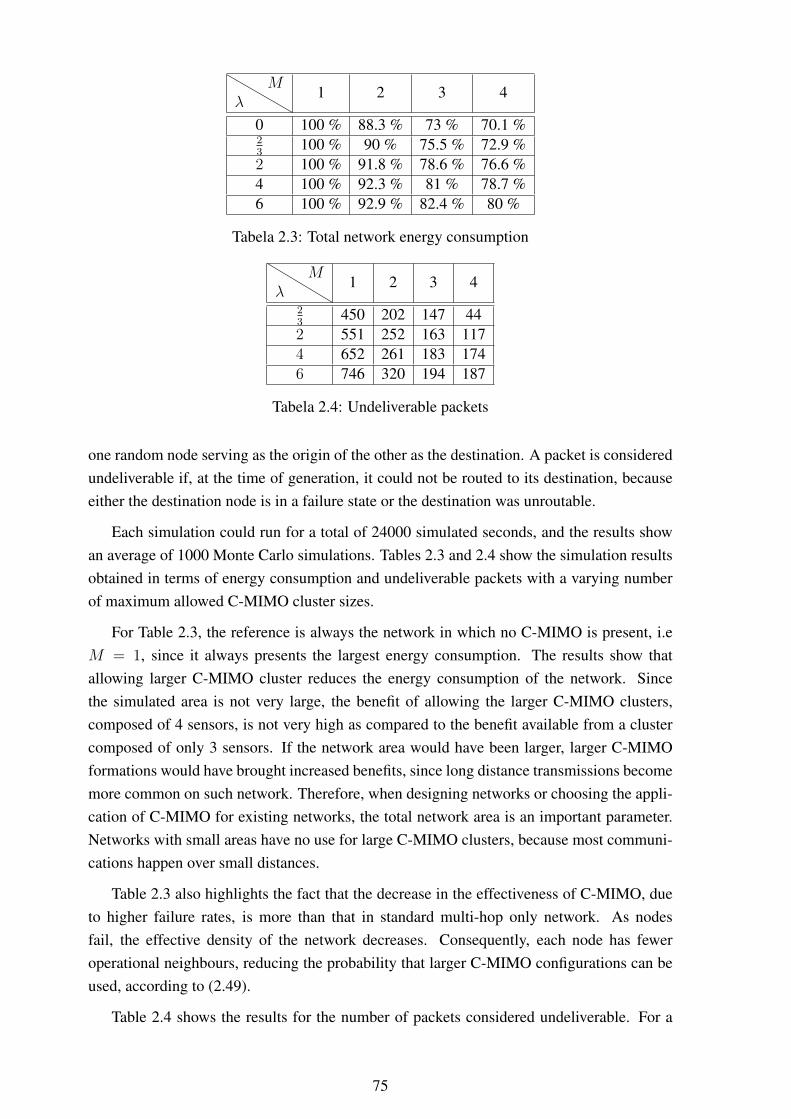
λM
1 2 3 4
0 100 % 88.3 % 73 % 70.1 %23
100 % 90 % 75.5 % 72.9 %2 100 % 91.8 % 78.6 % 76.6 %4 100 % 92.3 % 81 % 78.7 %6 100 % 92.9 % 82.4 % 80 %
Tabela 2.3: Total network energy consumption
λM
1 2 3 4
23
450 202 147 442 551 252 163 1174 652 261 183 1746 746 320 194 187
Tabela 2.4: Undeliverable packets
one random node serving as the origin of the other as the destination. A packet is consideredundeliverable if, at the time of generation, it could not be routed to its destination, becauseeither the destination node is in a failure state or the destination was unroutable.
Each simulation could run for a total of 24000 simulated seconds, and the results showan average of 1000 Monte Carlo simulations. Tables 2.3 and 2.4 show the simulation resultsobtained in terms of energy consumption and undeliverable packets with a varying numberof maximum allowed C-MIMO cluster sizes.
For Table 2.3, the reference is always the network in which no C-MIMO is present, i.eM = 1, since it always presents the largest energy consumption. The results show thatallowing larger C-MIMO cluster reduces the energy consumption of the network. Sincethe simulated area is not very large, the benefit of allowing the larger C-MIMO clusters,composed of 4 sensors, is not very high as compared to the benefit available from a clustercomposed of only 3 sensors. If the network area would have been larger, larger C-MIMOformations would have brought increased benefits, since long distance transmissions becomemore common on such network. Therefore, when designing networks or choosing the appli-cation of C-MIMO for existing networks, the total network area is an important parameter.Networks with small areas have no use for large C-MIMO clusters, because most communi-cations happen over small distances.
Table 2.3 also highlights the fact that the decrease in the effectiveness of C-MIMO, dueto higher failure rates, is more than that in standard multi-hop only network. As nodesfail, the effective density of the network decreases. Consequently, each node has feweroperational neighbours, reducing the probability that larger C-MIMO configurations can beused, according to (2.49).
Table 2.4 shows the results for the number of packets considered undeliverable. For a
75
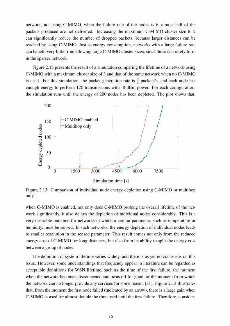
network, not using C-MIMO, when the failure rate of the nodes is 6, almost half of thepackets produced are not delivered. Increasing the maximum C-MIMO cluster size to 2can significantly reduce the number of dropped packets, because larger distances can bereached by using C-MIMO. Just as energy consumption, networks with a large failure ratecan benefit very little from allowing large C-MIMO cluster sizes, since those can rarely formin the sparser network.
Figure 2.13 presents the result of a simulation comparing the lifetime of a network usingC-MIMO with a maximum cluster size of 3 and that of the same network when no C-MIMOis used. For this simulation, the packet generation rate is 2
3packets/s, and each node has
enough energy to perform 120 transmissions with -8 dBm power. For each configuration,the simulation runs until the energy of 200 nodes has been depleted. The plot shows that,
Simulation time [s]
Ene
rgy
depl
eted
node
s
0
200
150
100
50
C-MIMO enabledMultihop only
01500 3000 4500 6000 7500
Figura 2.13: Comparison of individual node energy depletion using C-MIMO or multihoponly
when C-MIMO is enabled, not only does C-MIMO prolong the overall lifetime of the net-work significantly, it also delays the depletion of individual nodes considerably. This is avery desirable outcome for networks in which a certain parameter, such as temperature orhumidity, must be sensed. In such networks, the energy depletion of individual nodes leadsto smaller resolution in the sensed parameter. This result comes not only from the reducedenergy cost of C-MIMO for long distances, but also from its ability to split the energy costbetween a group of nodes.
The definition of system lifetime varies widely, and there is as yet no consensus on thisissue. However, some understandings that frequency appear in literature can be regarded asacceptable definitions for WSN lifetime, such as the time of the first failure, the momentwhen the network becomes disconnected and turns off for good, or the moment from whichthe network can no longer provide any services for some reason [31]. Figure 2.13 illustratesthat, from the moment the first node failed (indicated by an arrow), there is a large gain whenC-MIMO is used for almost double the time used until the first failure. Therefore, consider-
76

ing that the lifetime of a network ends with the first failure, the lifetime of the network underevaluation is doubled.
Figure 2.20 presents an example of a WSN with areas highlighted based on their ex-pected communication energy consumption. In this example, the center area, shown with acheckered background, is expected to expend more energy than the rest of the network dueto communication. The nodes that are located in the center are responsible for forwardinga large number of packets from nodes that are located closer to the edges of the network.Therefore, the nodes located in this area reach the end of their energy reserves faster thanthe rest of the network. On the other hand, nodes that are located on the stripped area havelonger lifetimes as these nodes are rarely responsible for routing information for other nodes.
Figures 2.21 and 2.22 highlight the effects of the proposed C-MIMO cluster formationon the available energy reserve of nodes located at the center and near the edges of thenetwork. The results shown in Figures 2.21 are expected, since the nodes that are locatedin the center have to perform less re-transmissions of data from other nodes on the network.Since C-MIMO can reach longer distances the nodes that generate the data can communicatewith more distant nodes without requiring a large number of intermediary hops. On the otherhand, while the results in Figure 2.22 show a decrease in the mean available energy for nodeslocated near the edges of the network. This, however, is desirable. The decrease in availableenergy indicates that the nodes located on the edges that, without C-MIMO, would generatepackets and hand them over for other nodes to transmit across the network are now ableto transmit over larger distances and spend their own energy reserves. This alleviates theenergetic strain on sensors located at the center of the network. The results also show that,if a fixed C-MIMO cluster size is used the center nodes have their energy reserves depletedfaster since fixing the cluster size prevents minimizing the energy consumption with respectto the distance between nodes.
Figures 2.23 and 2.24 present the effects of the proposed C-MIMO cluster formation onthe distribution of energy on the network. Figure 2.23 shows that when no C-MIMO is usedthe energy on the center is poorly distributed, illustrated by the large standard deviation σbetween the energy reserves of the nodes. Although the distribution seems to improve aftera certain instant, this is only true due to the fact that the nodes on the center are running outof energy, resulting in a smaller σ as the number of nodes with very small energy reservesgrows. Figure 2.24 shows that also for the edges of the network the energy distribution ismore uniform when the proposed algorithm is used.
The results of comparing energy dispersion can be further analysed by ploting the in-dividual energy reserves of nodes across the network. Figures 2.14, 2.16, and 2.18 showthe status of the energy available, in percentage, in the network nodes after 2500, 4500 and5500 seconds of simulation without enabling C-MIMO. Figures 2.15, 2.17, and 2.19 presentthe results in respect of the same parameters for a network after enabling the C-MIMO witha maximum cluster size of 3. Nodes with enough energy for at least one transmission areshown as circles and the depleted as diamond symbols. When no C-MIMO is used, the nodes
77
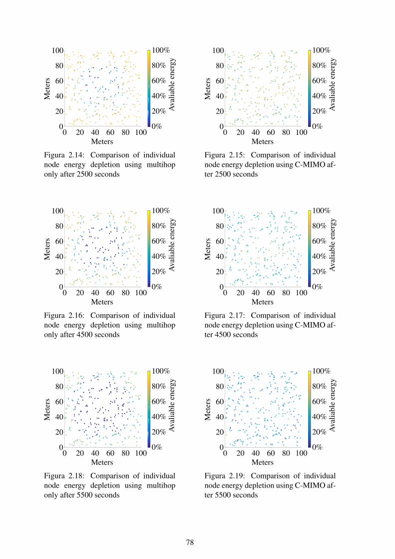
Meters0 20 40 60 80 100
Met
ers
0
20
40
60
80
100
Ava
liabl
een
ergy
0%
20%
40%
60%
80%
100%
Figura 2.14: Comparison of individualnode energy depletion using multihoponly after 2500 seconds
Meters0 20 40 60 80 100
Met
ers
0
20
40
60
80
100
Ava
liabl
een
ergy
0%
20%
40%
60%
80%
100%
Figura 2.15: Comparison of individualnode energy depletion using C-MIMO af-ter 2500 seconds
Meters0 20 40 60 80 100
Met
ers
0
20
40
60
80
100
Ava
liabl
een
ergy
0%
20%
40%
60%
80%
100%
Figura 2.16: Comparison of individualnode energy depletion using multihoponly after 4500 seconds
Meters0 20 40 60 80 100
Met
ers
0
20
40
60
80
100
Ava
liabl
een
ergy
0%
20%
40%
60%
80%
100%
Figura 2.17: Comparison of individualnode energy depletion using C-MIMO af-ter 4500 seconds
Meters0 20 40 60 80 100
Met
ers
0
20
40
60
80
100
Ava
liabl
een
ergy
0%
20%
40%
60%
80%
100%
Figura 2.18: Comparison of individualnode energy depletion using multihoponly after 5500 seconds
Meters0 20 40 60 80 100
Met
ers
0
20
40
60
80
100
Ava
liabl
een
ergy
0%
20%
40%
60%
80%
100%
Figura 2.19: Comparison of individualnode energy depletion using C-MIMO af-ter 5500 seconds
78
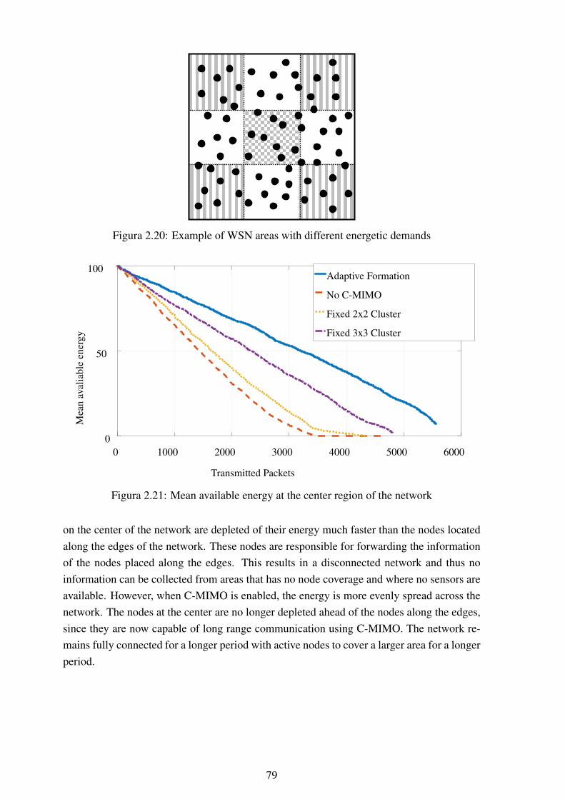
Figura 2.20: Example of WSN areas with different energetic demands
Transmitted Packets
0 1000 2000 3000 4000 5000 6000
Mea
nav
alia
ble
ener
gy
0
50
100Adaptive Formation
No C-MIMO
Fixed 2x2 Cluster
Fixed 3x3 Cluster
Figura 2.21: Mean available energy at the center region of the network
on the center of the network are depleted of their energy much faster than the nodes locatedalong the edges of the network. These nodes are responsible for forwarding the informationof the nodes placed along the edges. This results in a disconnected network and thus noinformation can be collected from areas that has no node coverage and where no sensors areavailable. However, when C-MIMO is enabled, the energy is more evenly spread across thenetwork. The nodes at the center are no longer depleted ahead of the nodes along the edges,since they are now capable of long range communication using C-MIMO. The network re-mains fully connected for a longer period with active nodes to cover a larger area for a longerperiod.
79
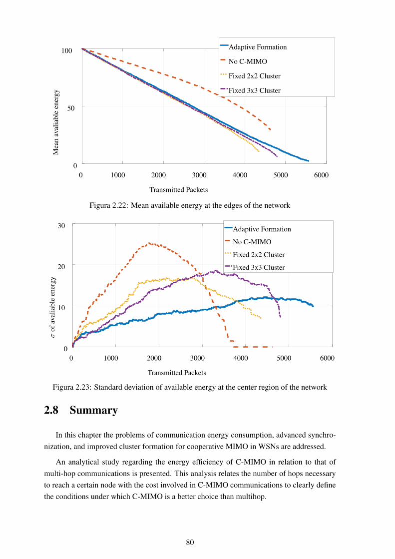
Transmitted Packets
0 1000 2000 3000 4000 5000 6000
Mea
nav
alia
ble
ener
gy
0
50
100 Adaptive Formation
No C-MIMO
Fixed 2x2 Cluster
Fixed 3x3 Cluster
Figura 2.22: Mean available energy at the edges of the network
Transmitted Packets
0 1000 2000 3000 4000 5000 6000
σof
aval
iabl
een
ergy
0
10
20
30 Adaptive Formation
No C-MIMO
Fixed 2x2 Cluster
Fixed 3x3 Cluster
Figura 2.23: Standard deviation of available energy at the center region of the network
2.8 Summary
In this chapter the problems of communication energy consumption, advanced synchro-nization, and improved cluster formation for cooperative MIMO in WSNs are addressed.
An analytical study regarding the energy efficiency of C-MIMO in relation to that ofmulti-hop communications is presented. This analysis relates the number of hops necessaryto reach a certain node with the cost involved in C-MIMO communications to clearly definethe conditions under which C-MIMO is a better choice than multihop.
80
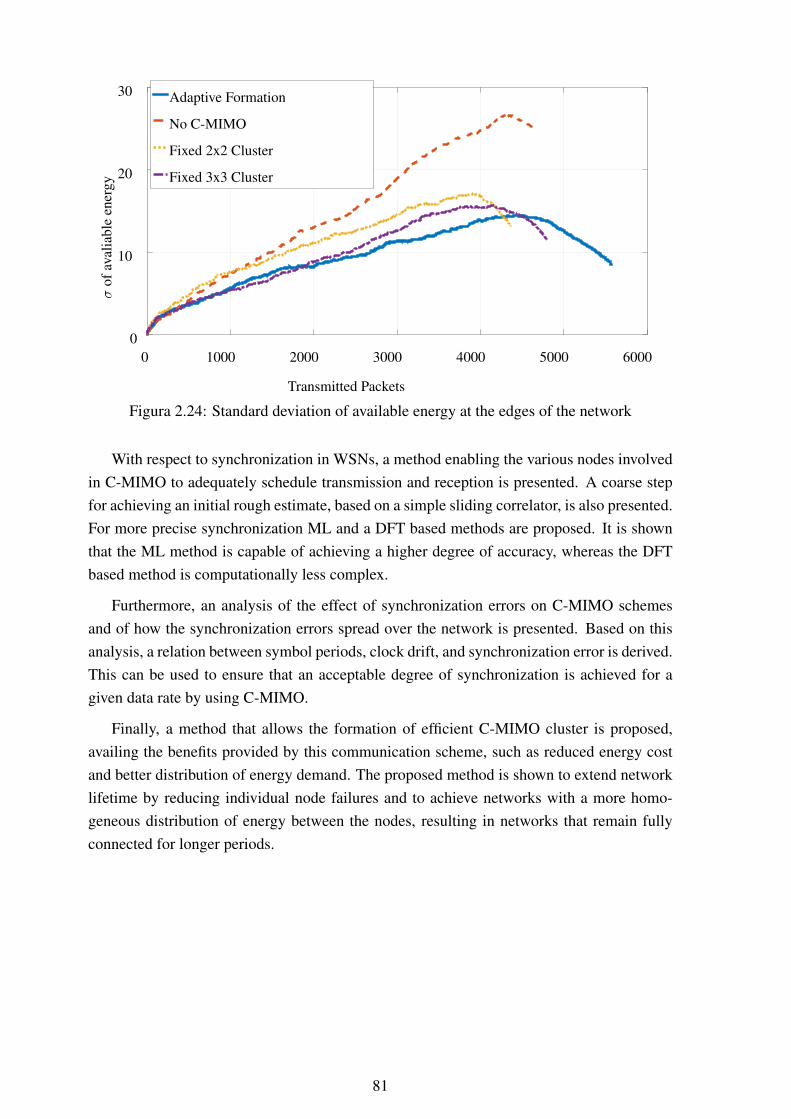
Transmitted Packets
0 1000 2000 3000 4000 5000 6000
σof
aval
iabl
een
ergy
0
10
20
30 Adaptive Formation
No C-MIMO
Fixed 2x2 Cluster
Fixed 3x3 Cluster
Figura 2.24: Standard deviation of available energy at the edges of the network
With respect to synchronization in WSNs, a method enabling the various nodes involvedin C-MIMO to adequately schedule transmission and reception is presented. A coarse stepfor achieving an initial rough estimate, based on a simple sliding correlator, is also presented.For more precise synchronization ML and a DFT based methods are proposed. It is shownthat the ML method is capable of achieving a higher degree of accuracy, whereas the DFTbased method is computationally less complex.
Furthermore, an analysis of the effect of synchronization errors on C-MIMO schemesand of how the synchronization errors spread over the network is presented. Based on thisanalysis, a relation between symbol periods, clock drift, and synchronization error is derived.This can be used to ensure that an acceptable degree of synchronization is achieved for agiven data rate by using C-MIMO.
Finally, a method that allows the formation of efficient C-MIMO cluster is proposed,availing the benefits provided by this communication scheme, such as reduced energy costand better distribution of energy demand. The proposed method is shown to extend networklifetime by reducing individual node failures and to achieve networks with a more homo-geneous distribution of energy between the nodes, resulting in networks that remain fullyconnected for longer periods.
81
Chapter 3
Array Processing Localization forVehicular Networks
In this chapter the following research question is addressed:Can array processing techniques be used to reliably estimate position of vehicles and pedes-trians in vehicular scenarios based on their radio transmissions?
3.1 Overview and Contribution
The remainder of this section is organized as follows:
• Motivation: The concept of vehicular networks and smart transportation systems isintroduced. The problem of localizing vehicles and road users in such environment isshown and a solution from an array processing perspective is introduced.
• Data Model: The broadband spherical wave data model of a signal received at anantenna array is defined.
• Space-Alternating Generalized Expectation Maximization (SAGE) Algorithm:Here, the space-alternating generalized expectation-maximization (SAGE) algorithmfor parameter estimation is briefly explained.
• Scenario Description: The assumed scenario for the localization in vehicular net-works is shown and some constraints are discussed.
• Array Processing Localization: In this section three different approaches for local-ization in vehicular scenarios are presented. These approaches vary in performanceand complexity and can be applied based on the specific performance and output raterequirements.
82
• Three Dimensional DOA Based Estimation: Here, the DOA based method is ex-tended to the three dimensional case considering the estimation of position and attitudeof UAVs as an application.
• Simulation Results: Finally, the performance of the proposed methods is shown bymeans of numerical simulations. A set of such simulations is performed using a realmeasured response from an antenna array to validate the proposed methods using realdata.
The research contributions presented in this chapter are:
1. A DOA only localization method capable of localizing transmitters near to a vehicleat a low computational cost.
2. A localization method based on range and DOA estimations performed at independentsubarrays. The geometrical relationship between the individual estimates is used tospeed up the rate of convergence of the SAGE algorithm on the individual subarrays.
3. A novel parametrization for the received waveform data model allowing joint localiza-tion estimation to be performed at both subarrays simultaneously.
4. Localization methods that do not require the transmission of specific location data thatcan be used to mitigate spoofing attacks in VANETs.
3.2 Motivation
Vehicular ad hoc networks (VANETs) are a promising technology with applications suchas road safety, traffic control, automated vehicle control, and platooning [60]. Many of suchapplications require the localization of all vehicles that compose a VANET to be knownor estimated with a high degree of accuracy. Furthermore, not only must the accuracy besufficient the estimate must also be reliable. Road safety, automated vehicles, and roadcontrol require the vehicles to be able to process and to estimate the position of vulnerableroad users (VRUs), as well as the position of the other vehicles in the vicinity, so that theycan operate adequately.
For the detection of VRUs, a variety of methods have been proposed. These methodsmust be precise and fast enough to meet different safety requirements regarding a multitudeof possible situations. A set of requirements for VRU detection systems is presented in [49].Most of these methods for VRU detection in the literature rely on computer vision [45].These methods can provide an accuracy of up to 75% [35, 46], which might be insufficientfor safety-critical systems such as collision detection and prevention/avoidance.
The localization of other vehicles is also of interest and can be obtained by using a va-riety of methods. One of the main source of location information in a VANET is the usage
83
of Global Navigation Satellite Systems (GNSS) information to obtain, for each vehicle, anestimate of it’s location. GNSS such as the Global Positioning System (GPS) can provide lo-cation information with a mean error of fifteen meters in urban environments [81]. However,this accuracy is not sufficient for emerging applications in Intelligent transportation systems(ITS) such as platooning [100] or for safety-critical applications. Furthermore, GNSS re-quires that a set of at least four line of sight signals are received from different satellites, thisis not always possible in dense urban environments, leading to a possible large number ofoutages.
Other means of vehicle positioning such as using the received signal strength indicator(RSSI) of the received data signals [86] can also be used and are capable of complement-ing GNSS information and making safety applications possible. Other vehicle positioningapproaches such as dead reckoning [57] can be used to provide position estimation duringoutages of GNSS. However, these approaches assume that the information that is providedby neighboring vehicles can be trusted.
Even in scenarios where the position provided by some vehicles can be assumed to bereliable and precise enough for the application at hand problems such as spoofing can stillemerge. In a spoofing attack it is possible to falsify GNSS information such that a vehiclewill obtain a position estimation that has been altered by the attacker. Furthermore, sinceGNSS information is usually spread using a data dissemination method [83], the positioninformation can be falsified by the transmitting vehicle or by intermediary vehicles of thenetwork. Position verification approaches [65] for VANETs can mitigate but not fully solvethe problem of spoofing attacks.
Approaches that leverage the presence of inertial sensors in smartphones inside a vehicle,using them to provide robust positioning for vehicles in a network have been proposed [22],providing an accuracy of approximately 7 meters. Methods for localization in vehicularnetworks based on building a social model of the interactions of vehicles in the networks canprovide position estimates with an accuracy of up to 10 meters [67]. While these methodsprovide an improvement over a GNSS only positioning solution, the accuracy provided isnot sufficient for the safety-critical applications in vehicular networks. Approaches that relyon a dedicated localization infrastructure can provide exact localization methods with anaccuracy superior to one meter [92] at the cost of an increased system complexity and maynot be available outside of urban and busy roads.
A promising technology that can be applied to VANETs is the Multiple-input multiple-output (MIMO) communication scheme. MIMO has been used in modern wireless commu-nications standards to allow for better spectral efficiency, faster data rates, and more robustcommunication. The usage of MIMO in vehicular network scenarios has been proposed toimprove the network performance [101], suppress possible jamming attacks [58], and in-crease network capacity [55]. The antennas used for MIMO applications can be leveragedto provide accurate positioning of vehicles on the network, without requiring a dedicatedinfrastructure. Since the usage of MIMO requires the presence of multiple antennas at both
84
receiver and transmitter, this antennas can be setup as, for instance, linear antenna arraysto allow the application of array signal processing techniques to provide an extra source oflocalization information on the network.
This work proposes the usage of array signal processing tools for direction of arrival(DOA) estimation to passively estimate the position of vehicles transmitting a signal. Theproposed method allows the position of a vehicle to be estimated by all vehicles within itscommunication range passively. This estimation does not require the transmission of local-ization specific messages, thus, it can be used to alleviate the network load. The proposedestimation method is also robust to data falsification since it relies on parameters that areestimated on the physical layer and cannot be altered or falsified easily, requiring a verycomplex system to do so.
3.3 Data Model
The assumed model considers a set ofLwavefronts impinging onto an ULA composed ofM antenna elements. The signal is assumed to be transmitted using an orthogonal frequency-division multiplexing (OFDM) scheme composed of K subcarriers. This model takes intoaccount the curvature of the spherical wavefront. Using the Fresnel approximation, afterremoving the cyclic prefix and taking the discrete Fourier transform (DFT) of the receivedsignal the space-frequency response of the k-th subcarrier received at antenna m during timesnapshot t can be written as
xm,k,t =L∑l=1
sl,k,tαm,l,keωl(m−1)+ψl(m−1)2 · ej2πk∆f (τl)
+ nm,k,t, (3.1)
where,
ωl = −2π∆m sin(θl)
λ, (3.2)
ψl =π∆2
m cos2(θl)
λrl, (3.3)
sl,k,t is the symbol transmitted by the l-th source at time instant t, αm,l,k is the complexchannel gain coefficient, ∆m is the separation between antenna elements of the array, θl isthe DOA of the l-th signal, rl is the range of the l-th source, λ is the wavelength of the carrierfrequency, ∆f is the frequency separation between the subcarriers of the OFDM signal, τlis the propagation delay of the l-th received signal, and nm,k,t is additive complex whiteGaussian noise.
85
The model can be rewritten in matrix form as
X = D(A � Z)S + N ∈ CMK×T , (3.4)
where � is the Khatri-Rao product, T is the total number of snapshots available, D is adiagonal matrix containing the channel gain coefficients, S ∈ CL×T contains the symbolstransmitted by the L sources for all T snapshots, N ∈ CMK×T is the noise matrix with itsentries drawn from CN (0, σ2
n), and
A = [a(θ1, r1), a(θ2, r2), ..., a(θL, rL)] ∈ CM×L, (3.5)
Z = [z(τ1), z(τ2), ..., z(τL)] ∈ CK×L, (3.6)
witha(θl, rl) =
[1, eωl+ψl , . . . , eωl(M−1)+ψl(M−1)2
]T
∈ CM×1, (3.7)
z(τl) =[ej2π1∆f (τl), ej2π2∆f (τl), . . . , ej2πK∆f (τl)
]T, ∈ CK×1, (3.8)
being the space and frequency steering vectors of the l-th received signal respectively.
3.4 Space-Alternating Generalized Expectation Maximiza-tion (SAGE) Algorithm
The SAGE algorithm is a generalization of the EM algorithm, both are algorithms usedto derive maximum likelihood estimates in an iterative fashion. The idea behind the thesealgorithms is to split an L-dimensional multi-dimensional problem that might be too com-putationally demanding to perform within an expected time constrain into L separate one-dimensional problems that can be solved within a shorter time. SAGE and EM utilize theconcept of hidden data space to avoid dealing with the complete observed data set. In thecase of a signal received at the array, the complete data can be written as a function of thehidden data space
Y = X1 + X2 + · · ·+ XL, (3.9)
Xl = h(pl)sl + nl, (3.10)
where h is a steering vector constructed from the parameter vector pl = [p1l , p
2l , . . . , p
Pl ], sl
is the symbol vector and n is the noise component and is complex normally distributed withzero mean and variance σ2
l .
86
An iteration of SAGE is split into two different steps, the expectation and the maximiza-tion steps. The expectation step of the c-th cycle of the i-th iteration of SAGE is given by
Xl(p[i,c−1]l , s
[i,c−1]l ) = E[Xl|Y,p
[i,c−1]l , s
[i,c−1]l ]
= h(p[i,c−1]l )s
[i,c−1]l
+1
L(Y −
L∑j=1j 6=i
h(p[i,c−1]j )s
[i,c−1]j ). (3.11)
RXl= Xl(p
[i,c−1]l , s
[i,c−1]l )Xl(p
[i,c−1]l , s
[i,c−1]l )H. (3.12)
The maximization step can then be performed, to estimate the parameter pjl the remainingparameters of p
[i,c−1]l are kept fixed and the following problem is solved
pjl[i,c]
= argmaxpjl
h(p[i,c−1]l )HRXl
(p[i,c−1]l , s
[i,c−1]l )h(p
[i,c−1]l ). (3.13)
The transmitted symbols are estimated following
s[i,c]l = h(p
[i,c]l )HXl(p
[i,c−1]l , s
[i,c−1]l ). (3.14)
The SAGE algorithm iterates over the parameters of all received signals until a conver-gence threshold is met. For the remainder of this work the superscripts for iteration and cyclewill be omitted to simplify the notation.
3.5 Scenario Description
This work assumes that the vehicles connected to the VANET are equipped with two lin-ear antenna arrays at two distinct locations on their frames. Figure 3.1 depicts an example ofa vehicle with antenna arrays equipped at the wing mirror position triangulating the positionof a VRU.
To avoid ambiguities in DOA estimation the antenna elements of the array must be placedno further than half a wave length apart. Assuming the communication occurs at the 5.8GHz frequency band and that DOA estimation is to be done at carrier frequency the antennaelements can be placed as far as 2.5 cm apart. Antenna elements can be installed closetogether to allow more antennas to be installed on the same area or to reduce the total sizeof the antenna array, however this comes at the cost of increasing mutual coupling betweenantenna elements. This work assumes that the antenna arrays are installed at the wing mirrorposition of the vehicles composing the network.
87
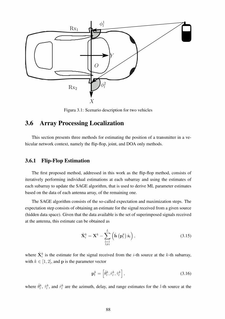
Rx1
Rx2
φ1l
φ2l
O
Y
X
Figura 3.1: Scenario description for two vehicles
3.6 Array Processing Localization
This section presents three methods for estimating the position of a transmitter in a ve-hicular network context, namely the flip-flop, joint, and DOA only methods.
3.6.1 Flip-Flop Estimation
The first proposed method, addressed in this work as the flip-flop method, consists ofiteratively performing individual estimations at each subarray and using the estimates ofeach subarray to update the SAGE algorithm, that is used to derive ML parameter estimatesbased on the data of each antenna array, of the remaining one.
The SAGE algorithm consists of the so-called expectation and maximization steps. Theexpectation step consists of obtaining an estimate for the signal received from a given source(hidden data space). Given that the data available is the set of superimposed signals receivedat the antenna, this estimate can be obtained as
Xki = Xk −
L∑l=1l 6=i
(h(pkl)sl
), (3.15)
where Xki is the estimate for the signal received from the i-th source at the k-th subarray,
with k ∈ [1, 2], and p is the parameter vector
pkl =[θkl , r
kl , τ
kl
], (3.16)
where θkl , τ kl , and rkl are the azimuth, delay, and range estimates for the l-th source at the
88

k-th subarray, respectively. sl is a vector with the estimates of the symbols transmitted bythe l-th source. Furthermore, h is the current estimate of h, which is defined as
h(pkl)
=[
a(θkl , r
kl
)⊗ z
(τ kl) ]∈ CMK×1. (3.17)
Following the expectation step, the maximization step transforms a D-dimensional esti-mation problem into D one-dimensional estimation problems by fixing all except one of theparameters during the estimation. Let the cost function d be defined as
d(pkl ,X
k)
=∣∣∣h (pkl )H
Xk∣∣∣2 . (3.18)
To obtain a complete estimate of p the algorithm will solve the set of D optimization prob-lems. These optimization problems can be written as
θkl = argmaxθkl
d(pkl , X
kl
), (3.19)
rkl = argmaxrkl
d(pkl , X
kl
), (3.20)
τ kl = argmaxτkl
d(pkl ,
ˆXkl
). (3.21)
To estimate each parameter, a different set of parameters is fixed, and a one-dimensionalsearch is performed over the parameter that is currently being estimated. This process isiteratively performed until the estimates of all parameters converges.
Once the range and DOA parameter has been estimated for one of the subarrays, anestimate of the position of the transmitter can be obtained. Assuming that the center of a linecrossing the car and both wing mirrors to be the origin of the reference coordinate system,denoted as O, it is necessary to obtain the angle φkl , which, as shown in Figure 3.1, is acomplementary angle to θkl . Thus, the relationship between φkl and θkl is given by
φkl = − 1
θkl + 2π. (3.22)
With this parameter at hand and following the coordinate system shown in Figure 3.1, anestimate of the position of the l-th transmitter with respect to the signal received at the k-thsubarray Rxk is given by
xkl = rkl cos(φkl ) + xRxk, (3.23)
ykl = rkl sin(φkl ). (3.24)
where xkl and ykl are the estimated coordinates for the position of the l-th transmitter. wherexRxl is the position of the center of the l-th antenna arrays over the X axis.
89
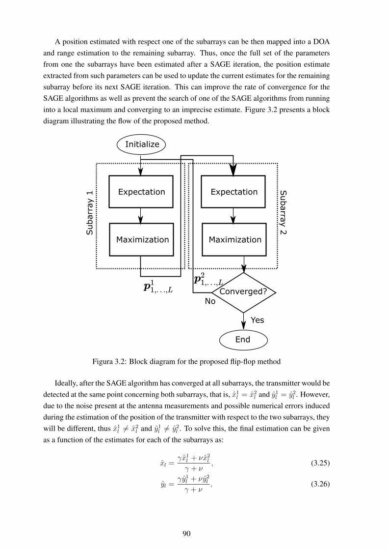
A position estimated with respect one of the subarrays can be then mapped into a DOAand range estimation to the remaining subarray. Thus, once the full set of the parametersfrom one the subarrays have been estimated after a SAGE iteration, the position estimateextracted from such parameters can be used to update the current estimates for the remainingsubarray before its next SAGE iteration. This can improve the rate of convergence for theSAGE algorithms as well as prevent the search of one of the SAGE algorithms from runninginto a local maximum and converging to an imprecise estimate. Figure 3.2 presents a blockdiagram illustrating the flow of the proposed method.
Expectation
Maximization
Expectation
Maximization
Initialize
Converged?No
End
Yes
Subarr
ay 1
Subarra
y 2
Figura 3.2: Block diagram for the proposed flip-flop method
Ideally, after the SAGE algorithm has converged at all subarrays, the transmitter would bedetected at the same point concerning both subarrays, that is, x1
l = x2l and y1
l = y2l . However,
due to the noise present at the antenna measurements and possible numerical errors inducedduring the estimation of the position of the transmitter with respect to the two subarrays, theywill be different, thus x1
l 6= x2l and y1
l 6= y2l . To solve this, the final estimation can be given
as a function of the estimates for each of the subarrays as:
xl =γx1
l + νx2l
γ + ν, (3.25)
yl =γy1
l + νy2l
γ + ν, (3.26)
90
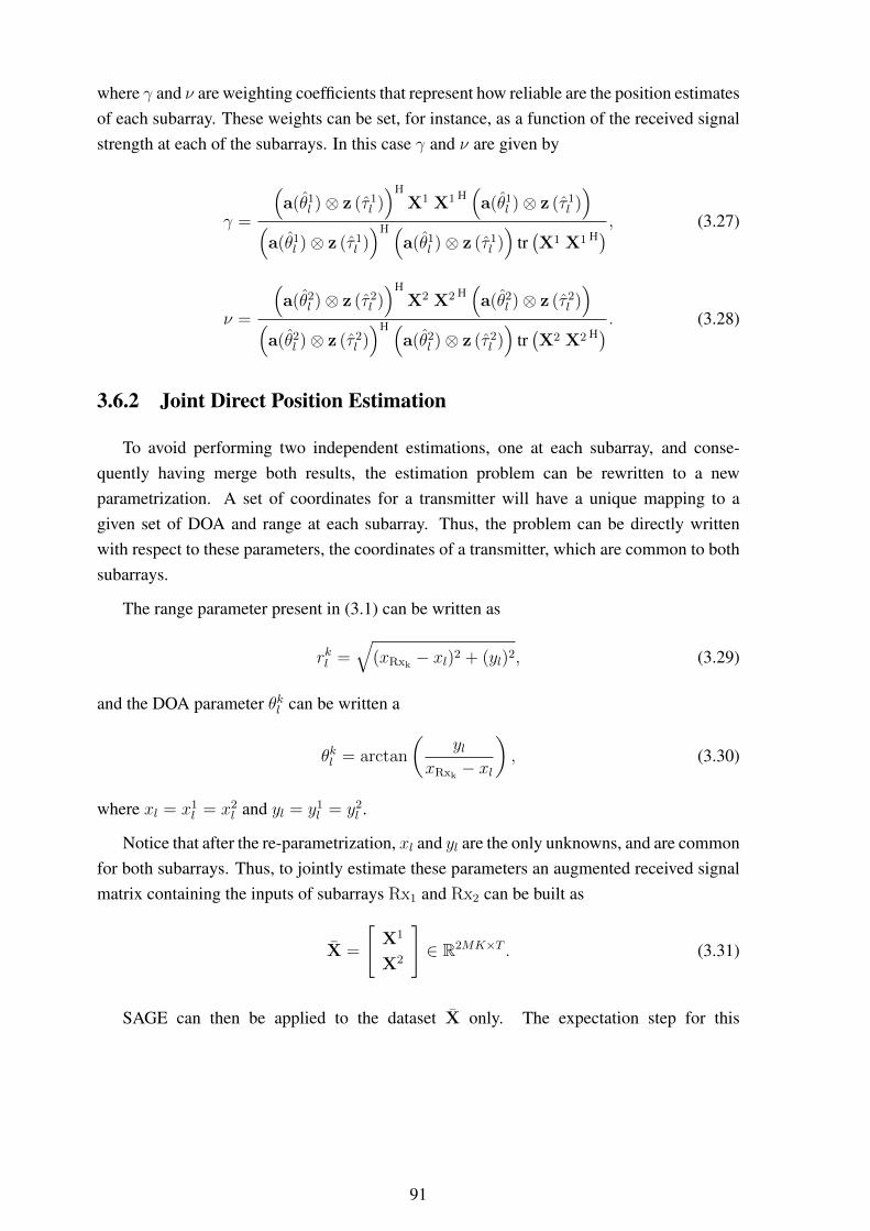
where γ and ν are weighting coefficients that represent how reliable are the position estimatesof each subarray. These weights can be set, for instance, as a function of the received signalstrength at each of the subarrays. In this case γ and ν are given by
γ =
(a(θ1
l )⊗ z (τ 1l ))H
X1 X1 H(a(θ1
l )⊗ z (τ 1l ))
(a(θ1
l )⊗ z (τ 1l ))H (
a(θ1l )⊗ z (τ 1
l ))
tr(X1 X1 H
) , (3.27)
ν =
(a(θ2
l )⊗ z (τ 2l ))H
X2 X2 H(a(θ2
l )⊗ z (τ 2l ))
(a(θ2
l )⊗ z (τ 2l ))H (
a(θ2l )⊗ z (τ 2
l ))
tr(X2 X2 H
) . (3.28)
3.6.2 Joint Direct Position Estimation
To avoid performing two independent estimations, one at each subarray, and conse-quently having merge both results, the estimation problem can be rewritten to a newparametrization. A set of coordinates for a transmitter will have a unique mapping to agiven set of DOA and range at each subarray. Thus, the problem can be directly writtenwith respect to these parameters, the coordinates of a transmitter, which are common to bothsubarrays.
The range parameter present in (3.1) can be written as
rkl =√
(xRxk− xl)2 + (yl)2, (3.29)
and the DOA parameter θkl can be written a
θkl = arctan
(yl
xRxk− xl
), (3.30)
where xl = x1l = x2
l and yl = y1l = y2
l .
Notice that after the re-parametrization, xl and yl are the only unknowns, and are commonfor both subarrays. Thus, to jointly estimate these parameters an augmented received signalmatrix containing the inputs of subarrays Rx1 and Rx2 can be built as
X =
[X1
X2
]∈ R2MK×T . (3.31)
SAGE can then be applied to the dataset X only. The expectation step for this
91
parametrization is given by
ˆXi = Xk −L∑l=1l 6=i
(h (pl) sl
), (3.32)
where pl is a unique parameter vector for both subarrays given by
pl = [xl, yl]. (3.33)
The cost function can then be written as
d(pl, X
)=∣∣∣h (pl)
H X∣∣∣2 . (3.34)
and the optimization problems can be solved directly for the transmitter coordinates xl andyl. Since the dataset of both subarrays is jointly used to perform the estimation, the distancebetween both subarrays is a contributing factor for the accuracy of the estimates obtained, asit improves the identifiability of the range parameter.
This method is, however, not without its drawbacks. The computational load when em-ploying the proposed joint estimation is higher than the computational load involved in theflip-flop method. The search space for the flip-flop method is limited to [−pi
2, pi
2] in the DOA
estimation, and to [0, rmax] in the range estimation, where rmax is the maximum assumedcommunication distance. For the joint estimation method, the search space is, in theory,[0, rmax] for both xl and yl, assuming that a transmitter can be located anywhere within asemicircle with radius rmax. While the search space may be reduced by assuming certainconstraints on a transmitting vehicle, it might lead to large biases in the presence of non-line-of-sight (NLOS) components that are not arriving from a position contained within thisreduced search space. Due to the restricted search space, such components will not be prop-erly estimated, and, therefore, their contribution to the received signal will not be properlyseparated from the remaining components, leading to possibly large estimation biases.
3.6.3 DOA only estimation
Alternatively, if a planar wavefront model is assumed, a position estimation for the trans-mitter can be obtained by performing individual parameter estimations at each of the subar-rays independently. In this case, the DOA estimation of an incoming signal at each of thesubarrays can be used to triangulate the transmitter, thus a narrowband model is sufficient.Notice that in this case, the phase delay factor ψl(m − 1)2 does not need to be consideredin (3.1), therefore it is not possible to obtain a direct ranging estimate. With DOA estimatesat hand and following the coordinate system shown in Figure 3.1 the lines representing the
92
signal received at Rx1 and Rx2 can be written as
y1l = tan(φ1
l )x1l − tan(φ1
l )xRx1 , (3.35)
y2l = tan(φ2
l )x2l − tan(φ2
l )xRx2 . (3.36)
The position of the transmitter array can be obtained by calculating the point where (3.35)and (3.36) intersect, this can be done by solving
xl =tan(φ1
l )xRx1 − tan(φ2l )xRx2
tan(φ1l )− tan(φ2
l ), (3.37)
yl =tan(φ1
l ) tan(φ2l ) (xRx2 − xRx1)
tan(φ2l )− tan(φ1
l ). (3.38)
While this method requires only DOA estimates at each of the subarrays to provide a po-sition estimate for the transmitter, it is highly sensitive to imprecisions in the DOA estimatesas it is a highly nonlinear function of these estimates.
3.6.4 Applicability of TDOA Estimation for Positioning
Another possible solution for estimating the position of a transmitter is to use the DOAsand TDOAs that have been estimated. Using the estimates of the time delay of arrival(TDOA) τ kl , an estimation of the range between the transmitting and receiving array canbe obtained as
rkl = cτ kl , (3.39)
where c is the speed of light. However, estimating the range by means of the TDOA is lessrobust than the one obtained trough the SAGE estimation using the spherical wave model.This is due to the fact that the TDOA can only be estimated with respect to an internal refer-ence at the receiver. That is, the TDOA estimation will be influenced by the synchronizationbetween the transmitter and the receiver. Whatever error is present in synchronization will bepresent in the TDOA estimation, as the internal reference of the receiver will differ from theone of the transmitter. Therefore, unless a very reliable source of synchronization is present,this method of positioning is not suitable for safety-critical applications, as a error in TDOAestimation of just one nano second will already result in a ranging error of approximately 30cm. If the synchronization between receiver and transmitter is to be relied on, the positionof the transmitter can be estimated following (3.23) and (3.24) and substituting the rangeestimate for the one shown in (3.39).
93
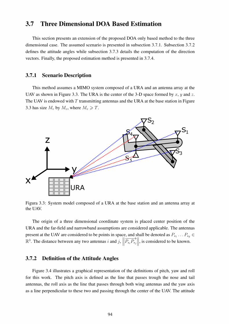
3.7 Three Dimensional DOA Based Estimation
This section presents an extension of the proposed DOA only based method to the threedimensional case. The assumed scenario is presented in subsection 3.7.1. Subsection 3.7.2defines the attitude angles while subsection 3.7.3 details the computation of the directionvectors. Finally, the proposed estimation method is presented in 3.7.4.
3.7.1 Scenario Description
This method assumes a MIMO system composed of a URA and an antenna array at theUAV as shown in Figure 3.3. The URA is the center of the 3-D space formed by x, y and z.The UAV is endowed with T transmitting antennas and the URA at the base station in Figure3.3 has size Mv by Mv, where Mv > T .
URA
S3
S2
S4S1
y
z
x
Figura 3.3: System model composed of a URA at the base station and an antenna array atthe UAV.
The origin of a three dimensional coordinate system is placed center position of theURA and the far-field and narrowband assumptions are considered applicable. The antennaspresent at the UAV are considered to be points in space, and shall be denoted as Ps1 . . . Psd ∈R3. The distance between any two antennas i and j,
∥∥∥−−−→PsiPsj
∥∥∥, is considered to be known.
3.7.2 Definition of the Attitude Angles
Figure 3.4 illustrates a graphical representation of the definitions of pitch, yaw and rollfor this work. The pitch axis is defined as the line that passes trough the nose and tailantennas, the roll axis as the line that passes through both wing antennas and the yaw axisas a line perpendicular to these two and passing through the center of the UAV. The attitude
94
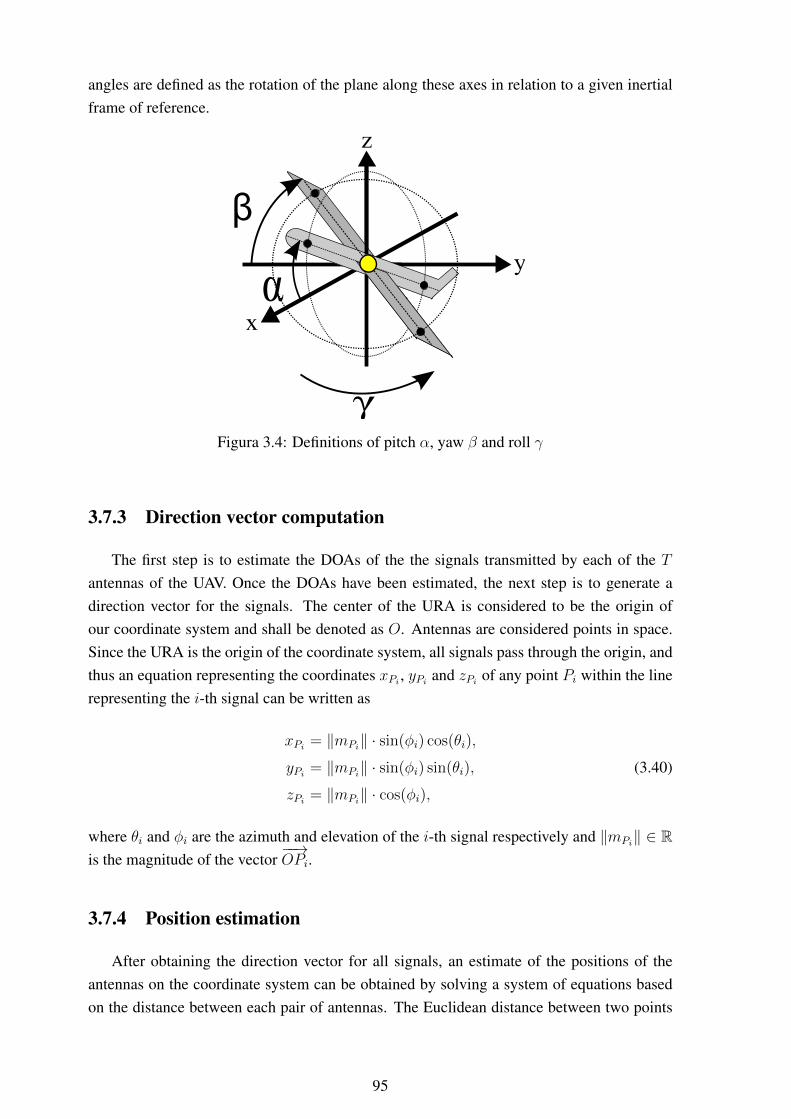
angles are defined as the rotation of the plane along these axes in relation to a given inertialframe of reference.
y
z
xα
γ
β
Figura 3.4: Definitions of pitch α, yaw β and roll γ
3.7.3 Direction vector computation
The first step is to estimate the DOAs of the the signals transmitted by each of the Tantennas of the UAV. Once the DOAs have been estimated, the next step is to generate adirection vector for the signals. The center of the URA is considered to be the origin ofour coordinate system and shall be denoted as O. Antennas are considered points in space.Since the URA is the origin of the coordinate system, all signals pass through the origin, andthus an equation representing the coordinates xPi , yPi and zPi of any point Pi within the linerepresenting the i-th signal can be written as
xPi = ‖mPi‖ · sin(φi) cos(θi),
yPi = ‖mPi‖ · sin(φi) sin(θi), (3.40)
zPi = ‖mPi‖ · cos(φi),
where θi and φi are the azimuth and elevation of the i-th signal respectively and ‖mPi‖ ∈ Ris the magnitude of the vector
−−→OPi.
3.7.4 Position estimation
After obtaining the direction vector for all signals, an estimate of the positions of theantennas on the coordinate system can be obtained by solving a system of equations basedon the distance between each pair of antennas. The Euclidean distance between two points
95
A ∈ R3 and B∈ R3 is given by
m−→AB
=√
(xA − xB)2 + (yA − yB)2 + (zA − zB)2. (3.41)
To find the estimate of the point where antennas i and j are located xA, xB, yA, yB, zAand zB can be replaced by xPi , xPj , yPi , yPj , zPi and zPj respectively. Since the distancesbetween each pair of antennas and the DOAs of each signal are known, ‖mPi‖ and
∥∥mPj
∥∥can be obtained, yielding an estimation of the positions of antennas i and j with respect tothe center of the URA. Note that there are n(n − 1)/2 available equations to choose from,where n is the number of antennas present at the UAV. Once the position of the antennas inthe UAV has been calculate, the TRIAD algorithm can be used to determine its attitude. TheTRIAD algorithm is detailed in Appendix H.
3.8 Simulation Results
This section presents a performance assessment of the proposed flip-flop and joint po-sitioning methods. Subsection 3.8.1 presents the results obtained for simulated data whilesubsection 3.8.2 presents the results obtained using measured data.
3.8.1 Results for Simulated Data
The performance of the proposed flip-flop and joint positioning algorithms is assessed bya set of numerical simulations. The simulation assumes two antenna subarrays at the wingmirrors; these are considered to be ULAs composed of M = 5 antennas with inner elementspacing of ∆m = λ
2. For the simulations, this work assumes the transmitter is using the LTE
standard, with the maximum fast Fourier transform size of 2048, of which 1200 are effec-tive subcarriers, and 15 kHz subcarrier spacing. Estimations are done assuming T = 100
OFDM symbols have been sampled with a normal cyclic prefix. Frequency correlation isintroduced by following the model proposed in [51]. To assess the performance of the pro-posed methods with respect to the bandwidth of the transmitted signal, a bandwidth rangingfrom a tonal signal (narrowband) to 20 MHz (largest possible LTE channel bandwidth) isconsidered. The ranging estimation is done only using the range parameter present in thespherical wave model, since the TDOA estimate reliability depends on the synchronizationbetween transmitter and receiver. The antenna arrays are assumed to be placed 1.80 m apartfrom each other, the average car width. Unless stated otherwise, the simulations assumethe presence of 3 non line of sight (NLOS) components with respective scatterers randomlyplaced between the transmitter and the receiving array. The number of components is notassumed to be known for the purposed of estimating the parameters using SAGE. Unlessstated otherwise, the Rician K factor for the simulations is kept fixed at 3 dB. The SAGEalgorithm for both the flip-flop and joint estimation methods is initialized using a position
96
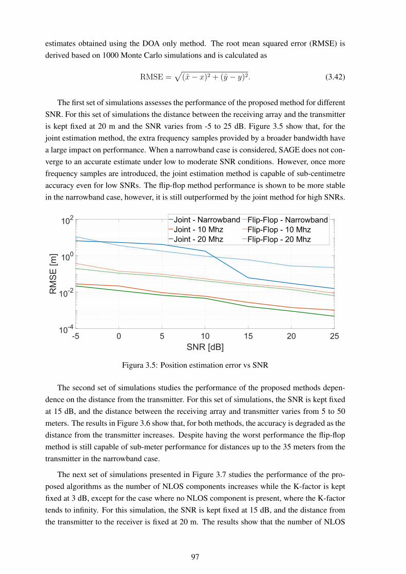
estimates obtained using the DOA only method. The root mean squared error (RMSE) isderived based on 1000 Monte Carlo simulations and is calculated as
RMSE =√
(x− x)2 + (y − y)2. (3.42)
The first set of simulations assesses the performance of the proposed method for differentSNR. For this set of simulations the distance between the receiving array and the transmitteris kept fixed at 20 m and the SNR varies from -5 to 25 dB. Figure 3.5 show that, for thejoint estimation method, the extra frequency samples provided by a broader bandwidth havea large impact on performance. When a narrowband case is considered, SAGE does not con-verge to an accurate estimate under low to moderate SNR conditions. However, once morefrequency samples are introduced, the joint estimation method is capable of sub-centimetreaccuracy even for low SNRs. The flip-flop method performance is shown to be more stablein the narrowband case, however, it is still outperformed by the joint method for high SNRs.
-5 0 5 10 15 20 25
SNR [dB]
10-4
10-2
100
102
RM
SE
[m
]
Joint - Narrowband
Joint - 10 Mhz
Joint - 20 Mhz
Flip-Flop - Narrowband
Flip-Flop - 10 Mhz
Flip-Flop - 20 Mhz
Figura 3.5: Position estimation error vs SNR
The second set of simulations studies the performance of the proposed methods depen-dence on the distance from the transmitter. For this set of simulations, the SNR is kept fixedat 15 dB, and the distance between the receiving array and transmitter varies from 5 to 50meters. The results in Figure 3.6 show that, for both methods, the accuracy is degraded as thedistance from the transmitter increases. Despite having the worst performance the flip-flopmethod is still capable of sub-meter performance for distances up to the 35 meters from thetransmitter in the narrowband case.
The next set of simulations presented in Figure 3.7 studies the performance of the pro-posed algorithms as the number of NLOS components increases while the K-factor is keptfixed at 3 dB, except for the case where no NLOS component is present, where the K-factortends to infinity. For this simulation, the SNR is kept fixed at 15 dB, and the distance fromthe transmitter to the receiver is fixed at 20 m. The results show that the number of NLOS
97
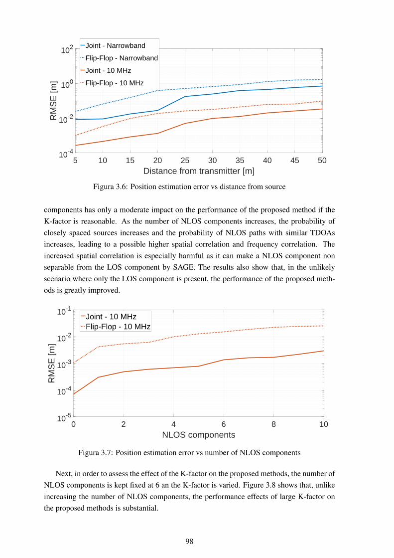
5 10 15 20 25 30 35 40 45 50Distance from transmitter [m]
10-4
10-2
100
102R
MS
E [m
]Joint - Narrowband
Flip-Flop - Narrowband
Joint - 10 MHz
Flip-Flop - 10 MHz
Figura 3.6: Position estimation error vs distance from source
components has only a moderate impact on the performance of the proposed method if theK-factor is reasonable. As the number of NLOS components increases, the probability ofclosely spaced sources increases and the probability of NLOS paths with similar TDOAsincreases, leading to a possible higher spatial correlation and frequency correlation. Theincreased spatial correlation is especially harmful as it can make a NLOS component nonseparable from the LOS component by SAGE. The results also show that, in the unlikelyscenario where only the LOS component is present, the performance of the proposed meth-ods is greatly improved.
0 2 4 6 8 10NLOS components
10-5
10-4
10-3
10-2
10-1
RM
SE
[m]
Joint - 10 MHzFlip-Flop - 10 MHz
Figura 3.7: Position estimation error vs number of NLOS components
Next, in order to assess the effect of the K-factor on the proposed methods, the number ofNLOS components is kept fixed at 6 an the K-factor is varied. Figure 3.8 shows that, unlikeincreasing the number of NLOS components, the performance effects of large K-factor onthe proposed methods is substantial.
98
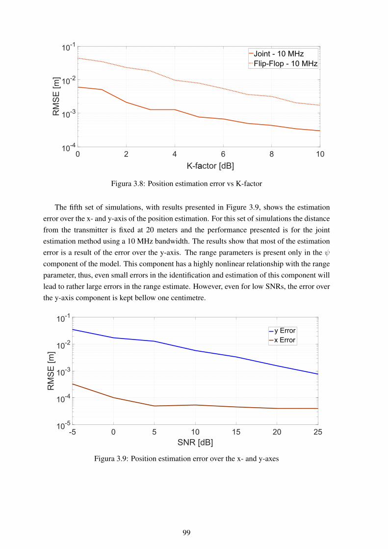
0 2 4 6 8 10
faactor [dB]K-
10-4
10-3
10-2
10-1
RM
SE
[m
]Joint - 10 MHz
Flip-Flop - 10 MHz
Figura 3.8: Position estimation error vs K-factor
The fifth set of simulations, with results presented in Figure 3.9, shows the estimationerror over the x- and y-axis of the position estimation. For this set of simulations the distancefrom the transmitter is fixed at 20 meters and the performance presented is for the jointestimation method using a 10 MHz bandwidth. The results show that most of the estimationerror is a result of the error over the y-axis. The range parameters is present only in the ψcomponent of the model. This component has a highly nonlinear relationship with the rangeparameter, thus, even small errors in the identification and estimation of this component willlead to rather large errors in the range estimate. However, even for low SNRs, the error overthe y-axis component is kept bellow one centimetre.
-5 0 5 10 15 20 25
SNR [dB]
10-5
10-4
10-3
10-2
10-1
RM
SE
[m
]
y Error
x Error
Figura 3.9: Position estimation error over the x- and y-axes
99

3.8.2 Results for Real Data
To assess the performance of the proposed method in real world scenarios, a measureddata set is used. The measurements were performed using a center frequency of 2.59 GHzwith 50 MHz of bandwidth. The antenna array is a ULA composed of 128 elements withinner element spacing of λ
2= 5.8cm and spanning 8 meters. Measurements were performed
at the Lund University Department of Computer Science. The antenna array was placed onthe roof of the entrance and the measurements were performed on a patio overlooked by thearray. Figures 3.10a and 3.10b present and overview of the placement of the antenna anda picture of the antenna array that was used for the measurements. Figure 3.11b presents amap of the location of users on the patio shown in Figure 3.11a with respect to the positionof the antenna array.
Antenna array
User locations
(a) Overview of measurement setup(b) Antenna array used for measurements
Figura 3.10: Antenna array and an overview of its placement
(a) Patio where measurements were per-formed
Ante
nna A
rray
(b) User distribution for measurements
Figura 3.11: Patio where measurements were performed and map of user distribution
100
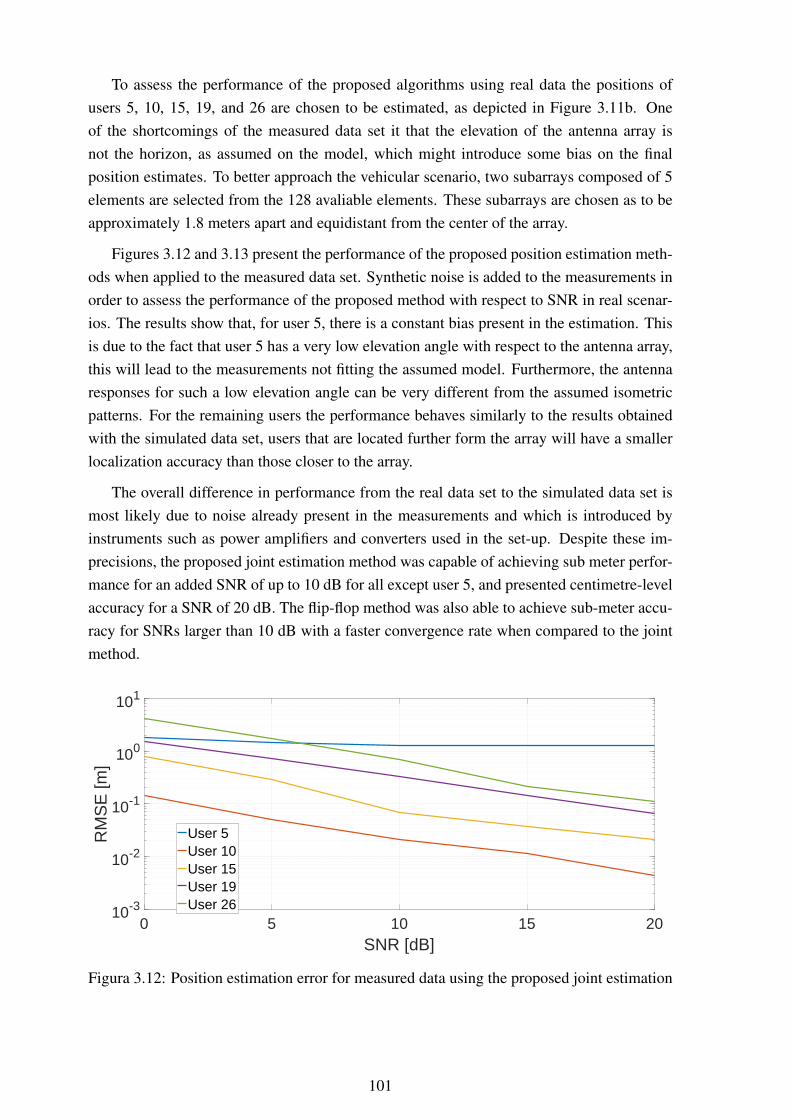
To assess the performance of the proposed algorithms using real data the positions ofusers 5, 10, 15, 19, and 26 are chosen to be estimated, as depicted in Figure 3.11b. Oneof the shortcomings of the measured data set it that the elevation of the antenna array isnot the horizon, as assumed on the model, which might introduce some bias on the finalposition estimates. To better approach the vehicular scenario, two subarrays composed of 5elements are selected from the 128 avaliable elements. These subarrays are chosen as to beapproximately 1.8 meters apart and equidistant from the center of the array.
Figures 3.12 and 3.13 present the performance of the proposed position estimation meth-ods when applied to the measured data set. Synthetic noise is added to the measurements inorder to assess the performance of the proposed method with respect to SNR in real scenar-ios. The results show that, for user 5, there is a constant bias present in the estimation. Thisis due to the fact that user 5 has a very low elevation angle with respect to the antenna array,this will lead to the measurements not fitting the assumed model. Furthermore, the antennaresponses for such a low elevation angle can be very different from the assumed isometricpatterns. For the remaining users the performance behaves similarly to the results obtainedwith the simulated data set, users that are located further form the array will have a smallerlocalization accuracy than those closer to the array.
The overall difference in performance from the real data set to the simulated data set ismost likely due to noise already present in the measurements and which is introduced byinstruments such as power amplifiers and converters used in the set-up. Despite these im-precisions, the proposed joint estimation method was capable of achieving sub meter perfor-mance for an added SNR of up to 10 dB for all except user 5, and presented centimetre-levelaccuracy for a SNR of 20 dB. The flip-flop method was also able to achieve sub-meter accu-racy for SNRs larger than 10 dB with a faster convergence rate when compared to the jointmethod.
0 5 10 15 20SNR [dB]
10-3
10-2
10-1
100
101
RM
SE
[m]
User 5User 10User 15User 19User 26
Figura 3.12: Position estimation error for measured data using the proposed joint estimation
101
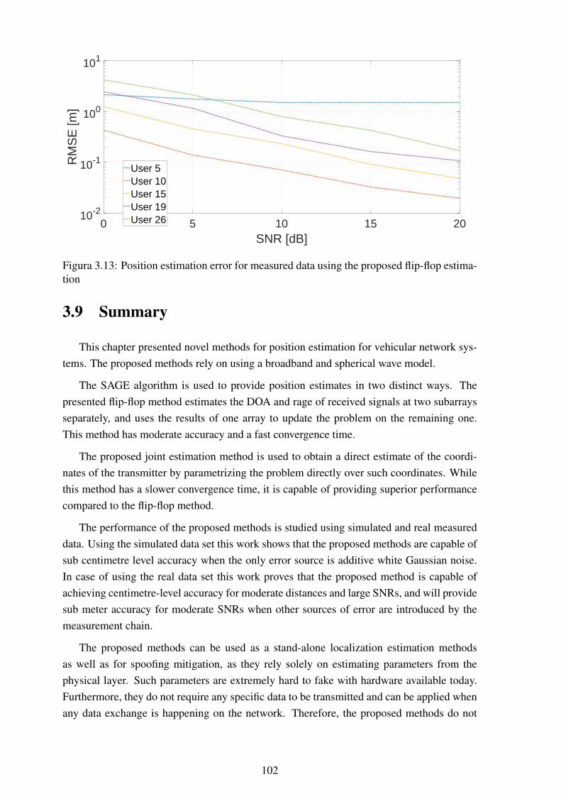
0 5 10 15 20SNR [dB]
10-2
10-1
100
101
RM
SE
[m]
User 5User 10User 15User 19User 26
Figura 3.13: Position estimation error for measured data using the proposed flip-flop estima-tion
3.9 Summary
This chapter presented novel methods for position estimation for vehicular network sys-tems. The proposed methods rely on using a broadband and spherical wave model.
The SAGE algorithm is used to provide position estimates in two distinct ways. Thepresented flip-flop method estimates the DOA and rage of received signals at two subarraysseparately, and uses the results of one array to update the problem on the remaining one.This method has moderate accuracy and a fast convergence time.
The proposed joint estimation method is used to obtain a direct estimate of the coordi-nates of the transmitter by parametrizing the problem directly over such coordinates. Whilethis method has a slower convergence time, it is capable of providing superior performancecompared to the flip-flop method.
The performance of the proposed methods is studied using simulated and real measureddata. Using the simulated data set this work shows that the proposed methods are capable ofsub centimetre level accuracy when the only error source is additive white Gaussian noise.In case of using the real data set this work proves that the proposed method is capable ofachieving centimetre-level accuracy for moderate distances and large SNRs, and will providesub meter accuracy for moderate SNRs when other sources of error are introduced by themeasurement chain.
The proposed methods can be used as a stand-alone localization estimation methodsas well as for spoofing mitigation, as they rely solely on estimating parameters from thephysical layer. Such parameters are extremely hard to fake with hardware available today.Furthermore, they do not require any specific data to be transmitted and can be applied whenany data exchange is happening on the network. Therefore, the proposed methods do not
102

imply an increased network load.
103
Conclusion
In this work the following research questions were tackled:
1. How to estimate the directions of arrival of correlated sources that are impinging onan antenna array that does not possess the necessary characteristics (geometry or elec-tromagnetic response) for doing so?
2. Can array processing techniques be used to provide improved lifetime and communi-cation performance in wireless sensor network?
3. Can array processing techniques be used to reliably estimate position of vehicles andpedestrians in vehicular scenarios based on their radio transmissions?
The first research question was addressed in Chapter 1. This chapter discussed two ap-proaches for sector detection and discretization, one approach is based on the UT while theother is based on the PCA. The presented approaches aim to preserve the statistical charac-teristics of the signal to be transformed while minimizing the transformation bias introducedin the process.
Linear array interpolation was discussed and an extension of linear interpolation to themultidimensional case was presented. The approach generalizes the problem of linear inter-polation to an arbitrary number of dimensions and allows the application of linear interpola-tion to arrays other than linear.
Two different alternatives for nonlinear array interpolation were also presented in Chap-ter 1. A way of performing array interpolation using the MARS method was presented.MARS is capable of expressing non-linear relationships between the real and the desiredresponse. MARS is shown to achieve good performance for larger SNRs and can provideperformances close to the CRLB. Furthermore, a novel approach for array interpolation ex-tending GRNNs to the problem of array interpolation was also presented. Using GRNNsallows the interpolation to take into account larger sectors of the field of view of the an-tenna array and to achieve DOA estimation results with smaller estimation error comparedto standard linear array interpolation. The proposed method is specially beneficial for arrayswith a limited number of elements or in the case where a larger number of signals is presentat the array, since in these cases the transformation error for the linear approach will lead toconsiderable bias in the DOA estimation. As it is possible to implement the proposed GRNN
104

array interpolation in a parallel manner, this leads to a fast interpolation especially suitablefor real time applications. While nonlinear methods are capable of providing an improve-ment of the linear interpolation, it is computationally expensive and does not always providea large improvement.
The performance of the proposed nonlinear interpolation methods was assessed using theresponse obtained from a real array. For such array, the proposed nonlinear methods werecapable of vastly outperforming their linear couterpart.
The second research question was addressed in Chapter 2, which presents a frameworkfor tackling practical problems for the implementation of C-MIMO in WSNs. The energyefficiency of C-MIMO in relation to that of multihop communications were studied andexpressions comparing the consumption of multi-hop and C-MIMO are derived. This allowsa routing mechanism to properly decide when to employ multi-hop or C-MIMO, achievingthe minimal possible energy consumption for data transmission.
A method allowing the various nodes involved in C-MIMO to properly schedule trans-mission and reception was presented. A simple sliding correlator synchronization methodwas also presented as means of achieving coarse synchronization. More precise synchroniza-tion methods based on ML and a DFT were presented. It was shown that the ML method iscapable of achieving a higher degree of accuracy, whereas the DFT based method is com-putationally less complex. Furthermore, an analysis of the effect of synchronization errorson C-MIMO schemes and of how the synchronization errors spread over the network waspresented. Based on this analysis, a relation between symbol periods, clock drift, and syn-chronization error was derived. This can be used to ensure that an acceptable degree ofsynchronization is achieved for a given data rate by using C-MIMO.
Also in Chapter 2, a method that allows the formation of efficient C-MIMO cluster wasproposed, availing the benefits provided by this communication scheme, such as reducedenergy cost and better distribution of energy demand. The proposed method was shown toextend network lifetime by reducing individual node failures and to achieve networks witha more homogeneous distribution of energy between the nodes, resulting in networks thatremain fully connected for longer periods.
The last research question was addressed in Chapter 3, where two different methodsfor position estimation in vehicular networks were presented. These methods rely on thepresence of separate antenna arrays on the frame of the vehicle and use a spherical wavemodel in order to estimate the position of a transmitter.
A fast converging flip-flop method that performs estimations of DOA and rage at eachsubarray individually was presented. This method uses the output of the estimation at eachsubarray to update the estimation problem on the remaining subarray. A joint estimationmethod, that uses the data of both subarrays simultaneously to estimate the coordinates ofthe transmitter directly was also presented. This method is capable of superior accuracywhen compared to the flip-flop method at the cost of increased convergence time.
105

Both methods were tested using simulated and a real measured data set. The simulateddata shows that the proposed methods are capable of centimetre level accuracy under idealconditions. The real data set shows that the proposed methods are still capable of achievingsub metre accuracy when other sources of error, such as the ones introduced by conversionand amplification, are present.
In summary, this work aimed to bring array processing closer to real life problems. Arrayinterpolation allows the application, in real systems, of signal processing tools that werepreviously confined to theory. Cooperative MIMO can be of great use to WSNs to extendtheir lifetime and, with that, their usability. Finally, array processing can be used to helpsolve the problem of localization in the context of vehicular networks, solving the problem ofreliability that is present when GPS or RSSI information is used. This can enable importanttechnologies such as automated driving and platooning to become a reality.
106
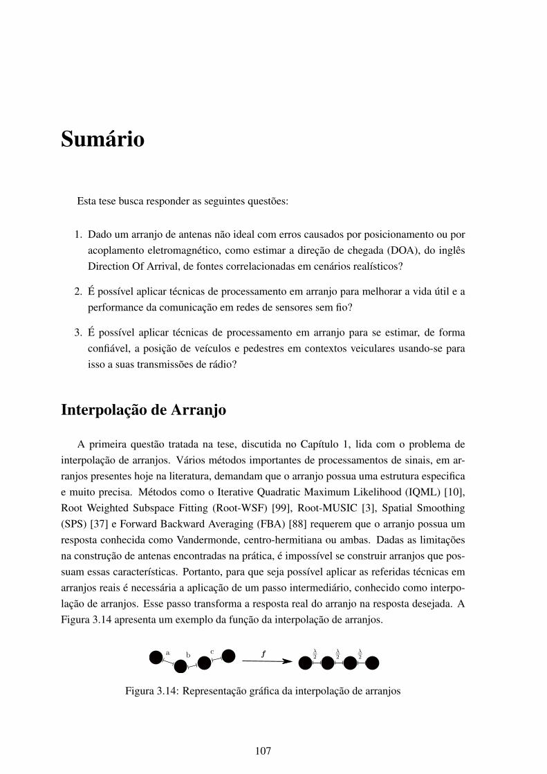
Sumário
Esta tese busca responder as seguintes questões:
1. Dado um arranjo de antenas não ideal com erros causados por posicionamento ou poracoplamento eletromagnético, como estimar a direção de chegada (DOA), do inglêsDirection Of Arrival, de fontes correlacionadas em cenários realísticos?
2. É possível aplicar técnicas de processamento em arranjo para melhorar a vida útil e aperformance da comunicação em redes de sensores sem fio?
3. É possível aplicar técnicas de processamento em arranjo para se estimar, de formaconfiável, a posição de veículos e pedestres em contextos veiculares usando-se paraisso a suas transmissões de rádio?
Interpolação de Arranjo
A primeira questão tratada na tese, discutida no Capítulo 1, lida com o problema deinterpolação de arranjos. Vários métodos importantes de processamentos de sinais, em ar-ranjos presentes hoje na literatura, demandam que o arranjo possua uma estrutura especificae muito precisa. Métodos como o Iterative Quadratic Maximum Likelihood (IQML) [10],Root Weighted Subspace Fitting (Root-WSF) [99], Root-MUSIC [3], Spatial Smoothing(SPS) [37] e Forward Backward Averaging (FBA) [88] requerem que o arranjo possua umresposta conhecida como Vandermonde, centro-hermitiana ou ambas. Dadas as limitaçõesna construção de antenas encontradas na prática, é impossível se construir arranjos que pos-suam essas características. Portanto, para que seja possível aplicar as referidas técnicas emarranjos reais é necessária a aplicação de um passo intermediário, conhecido como interpo-lação de arranjos. Esse passo transforma a resposta real do arranjo na resposta desejada. AFigura 3.14 apresenta um exemplo da função da interpolação de arranjos.
a b c λ2
λ2
λ2f
Figura 3.14: Representação gráfica da interpolação de arranjos
107
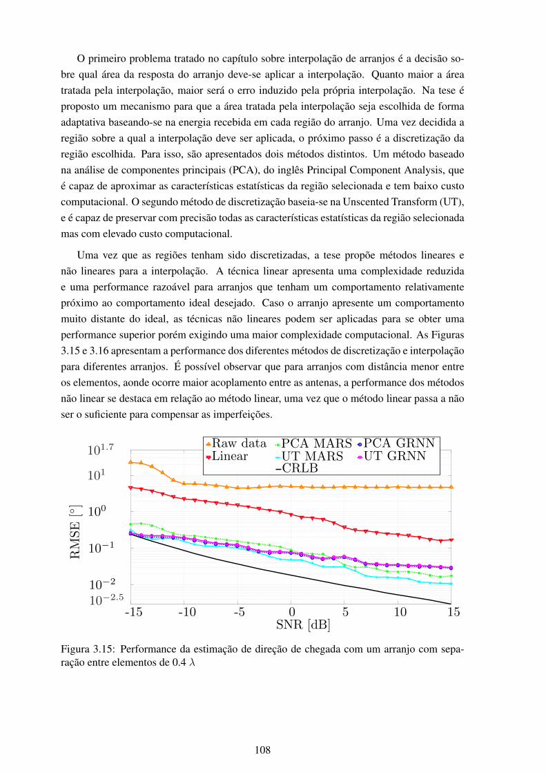
O primeiro problema tratado no capítulo sobre interpolação de arranjos é a decisão so-bre qual área da resposta do arranjo deve-se aplicar a interpolação. Quanto maior a áreatratada pela interpolação, maior será o erro induzido pela própria interpolação. Na tese éproposto um mecanismo para que a área tratada pela interpolação seja escolhida de formaadaptativa baseando-se na energia recebida em cada região do arranjo. Uma vez decidida aregião sobre a qual a interpolação deve ser aplicada, o próximo passo é a discretização daregião escolhida. Para isso, são apresentados dois métodos distintos. Um método baseadona análise de componentes principais (PCA), do inglês Principal Component Analysis, queé capaz de aproximar as características estatísticas da região selecionada e tem baixo custocomputacional. O segundo método de discretização baseia-se na Unscented Transform (UT),e é capaz de preservar com precisão todas as características estatísticas da região selecionadamas com elevado custo computacional.
Uma vez que as regiões tenham sido discretizadas, a tese propõe métodos lineares enão lineares para a interpolação. A técnica linear apresenta uma complexidade reduzidae uma performance razoável para arranjos que tenham um comportamento relativamentepróximo ao comportamento ideal desejado. Caso o arranjo apresente um comportamentomuito distante do ideal, as técnicas não lineares podem ser aplicadas para se obter umaperformance superior porém exigindo uma maior complexidade computacional. As Figuras3.15 e 3.16 apresentam a performance dos diferentes métodos de discretização e interpolaçãopara diferentes arranjos. É possível observar que para arranjos com distância menor entreos elementos, aonde ocorre maior acoplamento entre as antenas, a performance dos métodosnão linear se destaca em relação ao método linear, uma vez que o método linear passa a nãoser o suficiente para compensar as imperfeições.
-15 -10 -5 0 5 10 15
10−2
10−1
Raw dataLinear
PCA MARSUT MARS
PCA GRNNUT GRNN
CRLB
100
101
SNR [dB]
RMSE
[◦]
101.7
10−2.5
Figura 3.15: Performance da estimação de direção de chegada com um arranjo com sepa-ração entre elementos de 0.4 λ
108
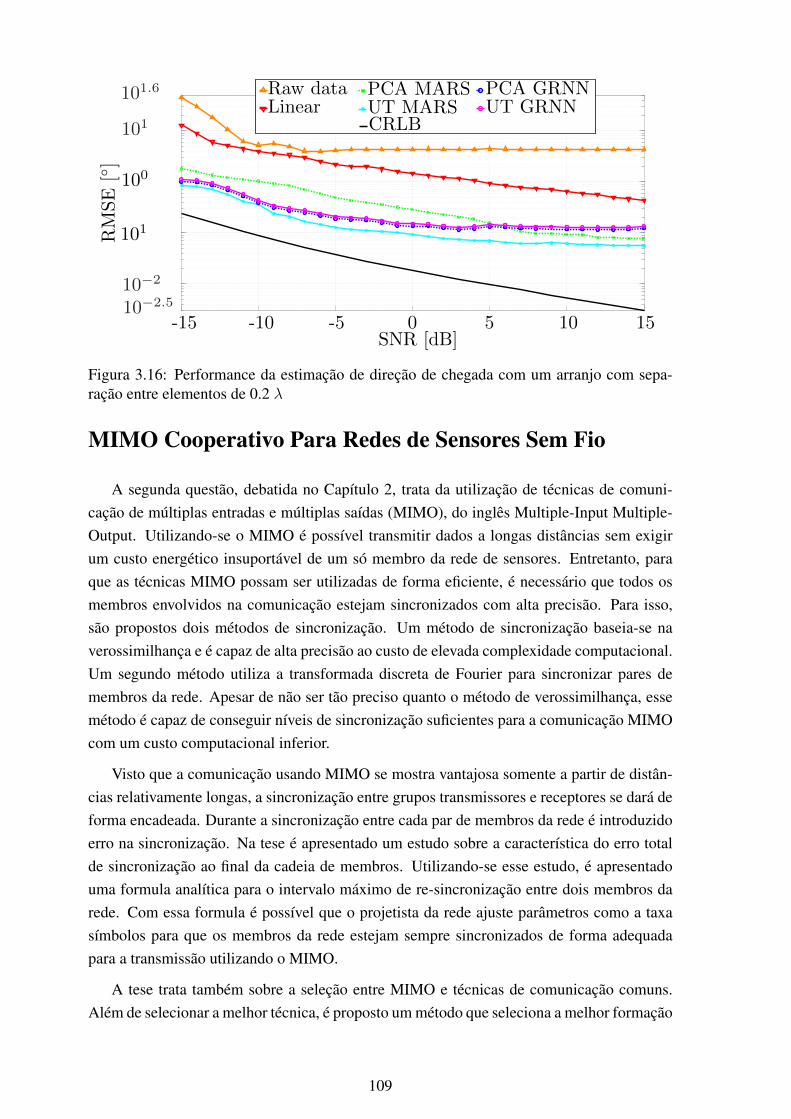
-15 -10 -5 0 5 10 15
Raw dataLinear
PCA MARSUT MARS
PCA GRNNUT GRNN
CRLB
10−2
101
100
101RMSE
[◦]
SNR [dB]
101.6
10−2.5
Figura 3.16: Performance da estimação de direção de chegada com um arranjo com sepa-ração entre elementos de 0.2 λ
MIMO Cooperativo Para Redes de Sensores Sem Fio
A segunda questão, debatida no Capítulo 2, trata da utilização de técnicas de comuni-cação de múltiplas entradas e múltiplas saídas (MIMO), do inglês Multiple-Input Multiple-Output. Utilizando-se o MIMO é possível transmitir dados a longas distâncias sem exigirum custo energético insuportável de um só membro da rede de sensores. Entretanto, paraque as técnicas MIMO possam ser utilizadas de forma eficiente, é necessário que todos osmembros envolvidos na comunicação estejam sincronizados com alta precisão. Para isso,são propostos dois métodos de sincronização. Um método de sincronização baseia-se naverossimilhança e é capaz de alta precisão ao custo de elevada complexidade computacional.Um segundo método utiliza a transformada discreta de Fourier para sincronizar pares demembros da rede. Apesar de não ser tão preciso quanto o método de verossimilhança, essemétodo é capaz de conseguir níveis de sincronização suficientes para a comunicação MIMOcom um custo computacional inferior.
Visto que a comunicação usando MIMO se mostra vantajosa somente a partir de distân-cias relativamente longas, a sincronização entre grupos transmissores e receptores se dará deforma encadeada. Durante a sincronização entre cada par de membros da rede é introduzidoerro na sincronização. Na tese é apresentado um estudo sobre a característica do erro totalde sincronização ao final da cadeia de membros. Utilizando-se esse estudo, é apresentadouma formula analítica para o intervalo máximo de re-sincronização entre dois membros darede. Com essa formula é possível que o projetista da rede ajuste parâmetros como a taxasímbolos para que os membros da rede estejam sempre sincronizados de forma adequadapara a transmissão utilizando o MIMO.
A tese trata também sobre a seleção entre MIMO e técnicas de comunicação comuns.Além de selecionar a melhor técnica, é proposto um método que seleciona a melhor formação
109

MIMO em relação não somente ao custo energético mas também em relação a distribuiçãoenergética da rede. Assim, é possível que os membros da rede esvaziem suas reservas en-ergéticas simultaneamente e não de forma individual, o que é desejável na maioria dos casospara redes de sensores.
As figuras 3.17, 3.18, 3.19, 3.20, 3.21 e 3.22 apresentam a distribuição energética deuma rede simulada utilizando apenas técnicas convencionais de comunicação e utilizandoos métodos propostos na tese. Os resultados demonstram que, utilizando-se os métodospropostos, a rede apresenta uma distribuição energética mais homogénea e se mantém com-pletamente conectada por mais tempo.
Localização via Processamento de Arranjo Para Redes Veic-ulares
A terceira questão, discutida no Capítulo 3, trata da localização de carros ou usuários deestradas vulneráveis (VRU), do inglês Vulnerable Road Users. Instalando-se dois arranjosde antenas em pontos distintos de um veículo, na tese presume-se que os arranjos estejaminstalados nos espelhos retrovisores, é possível levar em conta a curvatura da frente de ondatransmitida para se localizar o transmissor com precisão. Utilizando-se um modelo de dadosque leva em conta a curvatura esférica da onda transmitida, é possível se estiver não somentea direção de chegada mas também a distância do transmissor.
A tese apresenta três alternativas para a estimação da posição do transmissor. Uma al-ternativa utiliza somente as direções de chegada estimadas. Apesar de extremamente sim-ples, esse método é altamente vulnerável a imprecisões na estimação da direção de chegada.Levando-se em conta não somente a direção de chegada, mas também a distancia do trans-missor, é possível implementar-se um algoritmo iterativo entre os dois arranjos do veículo.Por ultimo, o método mais completo e complexo, leva em conta os dados recebidos nos doisarranjos simultaneamente. Esse método é capaz de alta performance ao custo de grandecomplexidade computacional.
As figuras 3.23 e 3.24 apresentam a performance dos métodos propostos utilizando-seum arranjo real e suas medições.
110
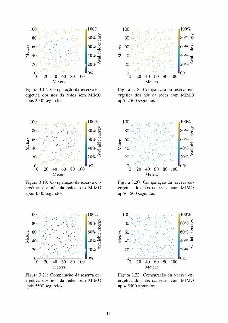
Meters0 20 40 60 80 100
Met
ers
0
20
40
60
80
100
Ava
liabl
een
ergy
0%
20%
40%
60%
80%
100%
Figura 3.17: Comparação da reserva en-ergética dos nós da redes sem MIMOapós 2500 segundos
Meters0 20 40 60 80 100
Met
ers
0
20
40
60
80
100
Ava
liabl
een
ergy
0%
20%
40%
60%
80%
100%
Figura 3.18: Comparação da reserva en-ergética dos nós da redes com MIMOapós 2500 segundos
Meters0 20 40 60 80 100
Met
ers
0
20
40
60
80
100
Ava
liabl
een
ergy
0%
20%
40%
60%
80%
100%
Figura 3.19: Comparação da reserva en-ergética dos nós da redes sem MIMOapós 4500 segundos
Meters0 20 40 60 80 100
Met
ers
0
20
40
60
80
100
Ava
liabl
een
ergy
0%
20%
40%
60%
80%
100%
Figura 3.20: Comparação da reserva en-ergética dos nós da redes com MIMOapós 4500 segundos
Meters0 20 40 60 80 100
Met
ers
0
20
40
60
80
100
Ava
liabl
een
ergy
0%
20%
40%
60%
80%
100%
Figura 3.21: Comparação da reserva en-ergética dos nós da redes sem MIMOapós 5500 segundos
Meters0 20 40 60 80 100
Met
ers
0
20
40
60
80
100
Ava
liabl
een
ergy
0%
20%
40%
60%
80%
100%
Figura 3.22: Comparação da reserva en-ergética dos nós da redes com MIMOapós 5500 segundos
111
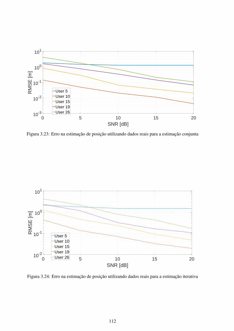
0 5 10 15 20SNR [dB]
10-3
10-2
10-1
100
101
RM
SE
[m]
User 5User 10User 15User 19User 26
Figura 3.23: Erro na estimação de posição utilizando dados reais para a estimação conjunta
0 5 10 15 20SNR [dB]
10-2
10-1
100
101
RM
SE
[m]
User 5User 10User 15User 19User 26
Figura 3.24: Erro na estimação de posição utilizando dados reais para a estimação iterativa
112

Author’s Publications
[ath1] S. Caizzone, W. Elmarissi, M. A. M. Marinho, and F. Antreich. Direction of arrivalestimation performance for compact antenna arrays with adjustable size. The IEEEInternational Microwave Symposium (IMS2017), 2017.
[ath2] E. P. de Freitas, R. K. Miranda, M. A. M. Marinho, J. P. C. L. da Costa, and C. E.Pereira. A practical implementation of a cooperative antenna array for wireless sensornetworks. In Conference on Smart Spaces, pages 309–318. Springer, 2015.
[ath3] E. P. Freitas, J. P. C. L. Costa, A. L. F. Almeida, and M. A. M. Marinho. ApplyingMIMO techniques to minimize energy consumption for long distances communica-tions in wireless sensor networks. In Springer-Verlag, editor, NEW2AN/ruSMART2012, pages 379–390, 2012.
[ath4] J. Milanezi Jr, J. P. C. L. da Costa, R. S. Ferreira Junior, M. A. M. Marinho, R. A.Shayani, and R. T. de Sousa Júnior. Energy harvesting photovoltaic system to chargea cell phone in indoor environments. In International Conference on Composite Ma-terials & Renewable Energy Applications 2014, 2014.
[ath5] R. S. Ferreira Jr., M. A. M. Marinho, K. Liu, J. P. C. L. da Costa, A. V. Amaral, andH. C. So. Improved landing radio altimeter for unmanned aerial vehicles based on anantenna array. 2012.
[ath6] J. P. A. Maranhão, J. P. C. L. da Costa, E. P. de Freitas, M. A. M. Marinho, andG. Del Galdo. Multi-hop cooperative XIXO transmission scheme for delay tolerantwireless sensor networks. In Smart Antennas (WSA 2016); Proceedings of the 20thInternational ITG Workshop on, pages 1–5. VDE, 2016.
[ath7] M. A. M. Marinho, F. Antreich, S. Caizzone, J. P. C. L. da Costa, A. Vinel, and E. P.de Freitas. Robust nonlinear array interpolation for direction of arrival estimation ofhighly correlated signals. Signal Processing, 144:19–28, 2018.
[ath8] M. A. M. Marinho, F. Antreich, and J. P. C. L. da Costa. Improved array interpo-lation for reduced bias in DOA estimation for gnss. In The Institute of Navigation,International Technical Meeting (ION ITM) 2014, 2014.
113

[ath9] M. A. M. Marinho, F. Antreich, J. P. C. L. da Costa, and J. A. Nossek. Reduced ranktls array interpolation for DOA estimation. In 18th International ITG Workshop onSmart Antennas (WSA 2014), 2014.
[ath10] M. A. M. Marinho, F. Antreich, J. P. C. L. da Costa, and J. A. Nossek. A signaladaptive array interpolation approach with reduced transformation bias for DOA es-timation of highly correlated signals. In Acoustics, Speech, and Signal Processing,2004. Proceedings. (ICASSP ’14). IEEE International Conference on, 2014.
[ath11] M. A. M. Marinho, J. P. C. L. da Costa, F. Antreich, A. L. F. de Almeida,G. Del Galdo, E. P. de Freitas, and A. Vinel. Array interpolation based on multivari-ate adaptive regression splines. In Sensor Array and Multichannel Signal ProcessingWorkshop (SAM), 2016 IEEE, pages 1–5. IEEE, 2016.
[ath12] M. A. M. Marinho, J. P. C. L. da Costa, F. Antreich, E. P. de Freitas, and A. Vinel.Adaptive communication and cooperative MIMO cluster formation for improved life-time in wireless sensor networks. In 2016 IEEE International Conference on Wirelessfor Space and Extreme Environments (WiSEE), Aachen, Germany, September 26-29,2016, 2016.
[ath13] M. A. M. Marinho, J. P. C. L. da Costa, F. Antreich, and L. R. A. X. de Menezes.Unscented transformation based array interpolation. In Proc. 40th International Con-ference on Acoustics, Speech, and Signal Processing (ICASSP), Brisbane, Australia,April 2015.
[ath14] M. A. M. Marinho, J. P. C. L. da Costa, F.Antreich, and L. R. A. X. de Menezes.Multidimensional array interpolation applied to direction of arrival estimation. In19th International ITG Workshop on Smart Antennas (WSA 2015), 2015.
[ath15] M. A. M. Marinho, E. P. de Freitas, J. P. C. L. da Costa, A. L. F. de Almeida, andR. T. de Sousa Jr. Using cooperative MIMO techniques and UAV relay networks tosupport connectivity in sparse wireless sensor networks. In Computing, Managementand Telecommunications (ComManTel), 2013 International Conference on, 2013.
[ath16] M. A. M. Marinho, E. P. de Freitas, J. P. C. L. da Costa, A. L. F. de Almeida, andR. T. de Sousa Jr. Using MIMO techniques to enhance communication among staticand mobile nodes in wireless sensor networks. In Advanced Information Networkingand Applications (AINA), 2013 IEEE 27th International Conference on, 2013.
[ath17] M. A. M. Marinho, E. P. de Freitas, J. P. C. L. da Costa, and R. T. de Sousa Jr.Applying cooperative MIMO technique in an adaptive routing mechanism for wire-less sensor networks. In 2013 IEEE Conference on Wireless Sensors (ICWiSe2013),2013.
114

[ath18] M. A. M. Marinho, E. P. de Freitas, J. P. C. L. da Costa, and R. T.de Sousa Jr. Synchronization for cooperative MIMO in wireless sensor networks.In NEW2AN/ruSMART 2013, 2013.
[ath19] M. A. M. Marinho, E. P. de Freitas, J. P. C. L. da Costa, and R. T. de Sousa Jr.Sensor localization via diversely polarized antennas. In International Workshop onPerformance Control in Wireless Sensor Networks (PWSN), 2014.
[ath20] M. A. M. Marinho, R. S. Ferreira Jr., J. P.C. L. da Costa, E. P. de Freitas, K. Liu,H. C. So, and F. Antreich. Antenna array based positioning scheme for unmannedaerial vehicles. In 17th International ITG Workshop on Smart Antennas (WSA 2013),2013.
[ath21] M. A. M. Marinho, A. Vinel, F. Antreich, J. P. C. L. da Costa, and E. P. de Freitas.Antenna array based localization scheme for vehicular networks. In Computer andInformation Technology (CIT), 2017 IEEE International Conference on, pages 142–146. IEEE, 2017.
[ath22] R. K. Miranda, J. P. C. L. da Costa, M. A. M. Marinho, E. P. de Freitas, and R. T.de Sousa Jr. Evaluation of space-time-frequency (stf)-coded MIMO-OFDM systemsin realistic channel models. In 28th IEEE International Conference on AdvancedInformation Networking and Applications (AINA-2014), 2014.
115
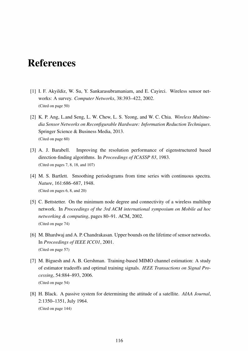
References
[1] I. F. Akyildiz, W. Su, Y. Sankarasubramaniam, and E. Cayirci. Wireless sensor net-works: A survey. Computer Networks, 38:393–422, 2002.(Cited on page 50)
[2] K. P. Ang, L.and Seng, L. W. Chew, L. S. Yeong, and W. C. Chia. Wireless Multime-dia Sensor Networks on Reconfigurable Hardware: Information Reduction Techniques.Springer Science & Business Media, 2013.(Cited on page 60)
[3] A. J. Barabell. Improving the resolution performance of eigenstructured baseddirection-finding algorithms. In Proceedings of ICASSP 83, 1983.(Cited on pages 7, 8, 18, and 107)
[4] M. S. Bartlett. Smoothing periodograms from time series with continuous spectra.Nature, 161:686–687, 1948.(Cited on pages 6, 8, and 20)
[5] C. Bettstetter. On the minimum node degree and connectivity of a wireless multihopnetwork. In Proceedings of the 3rd ACM international symposium on Mobile ad hocnetworking & computing, pages 80–91. ACM, 2002.(Cited on page 74)
[6] M. Bhardwaj and A. P. Chandrakasan. Upper bounds on the lifetime of sensor networks.In Proceedings of IEEE ICC01, 2001.(Cited on page 57)
[7] M. Biguesh and A. B. Gershman. Training-based MIMO channel estimation: A studyof estimator tradeoffs and optimal training signals. IEEE Transactions on Signal Pro-cessing, 54:884–893, 2006.(Cited on page 54)
[8] H. Black. A passive system for determining the attitude of a satellite. AIAA Journal,2:1350–1351, July 1964.(Cited on page 144)
116

[9] H. Black. Early developments of transit, the navy navigation satellite system. Journalof Guidance, Control and Dynamics, 13:577–585, July 1990.(Cited on page 144)
[10] Y. Bresler and A. Macovski. Exact maximum likelihood estimation of superimposedexponentials signals in noise. IEEE ASSP Magazine, 34:1081–189, 1986.(Cited on pages 7, 8, and 107)
[11] T. P. Bronez. Sector interpolation of non-uniform arrays for efficient high resolutionbearing estimation. In Acoustics, Speech, and Signal Processing, 1988. ICASSP-88.,1988 International Conference on, 1988.(Cited on pages 8, 24, and 27)
[12] M. Buhren, M. Pesavento, and J. F. Bohme. A new approach to array interpolation bygeneration of artificial shift invariances: Interpolated ESPRIT. In Acoustics, Speech,and Signal Processing, 2003. Proceedings. (ICASSP ’03). 2003 IEEE InternationalConference on, 2003.(Cited on pages 8, 14, and 19)
[13] M. Buhren, M. Pesavento, and J. F Böhme. Virtual array design for array interpolationusing differential geometry. In Acoustics, Speech, and Signal Processing, 2004. Pro-ceedings. (ICASSP ’04). IEEE International Conference on, volume 2, 2004.(Cited on pages 8 and 18)
[14] S. Caizzone and A. Dreher. Miniaturized DRA array for GNSS applications. In 20159th European Conference on Antennas and Propagation (EuCAP), pages 1–2. IEEE,2015.(Cited on page 42)
[15] S. Caizzone, W. Elmarissi, M. A. M. Marinho, and F. Antreich. Direction of arrivalestimation performance for compact antenna arrays with adjustable size. The IEEEInternational Microwave Symposium (IMS2017), 2017.(Cited on page 42)
[16] J. Capon. High-resolution frequency-wavenumber spectrum analysis. ProceedingsIEEE, 57:1408–1418, 1969.(Cited on pages 7, 8, and 22)
[17] C. Chen, J. Ma, and K. Yu. Designing energy-efficient wireless sensor networks withmobile sinks. In Sensys06, 2006.(Cited on pages 50 and 56)
[18] S. Cho and A. Chandrakasan. Energy-efficient protocols for low duty cycle wirelessmicrosensor. In Proceedings of the 33rd Annual Hawaii International Conference onSystem Sciences, 2000.(Cited on page 50)
117

[19] P. J. Chung and J. F. Böhme. Comparative convergence analysis of EM and SAGEalgorithms in DOA estimation. IEEE Transactions on Signal Processing, 49:2940–2949, 2001.(Cited on page 6)
[20] D. S. J. D. Couto, D. Aguayo, J. Bicket, and R. Morris. A high-throughput path metricfor multi-hop wireless routing. Wirel. Netw, 11:419–435, 2005.(Cited on page 55)
[21] J. H. Cozzens and M. J. Sousa. Source enumeration in a correlated signal environment.IEEE Transactions on Acoustics Speech and Signal Processing, 42:304–317, 1994.(Cited on page 13)
[22] S. B. Cruz, T. E. Abrudan, Z. Xiao, N. Trigoni, and J. Barros. Neighbor-aided localiza-tion in vehicular networks. IEEE Transactions on Intelligent Transportation Systems,2017.(Cited on page 84)
[23] S. Cui and A. J. Goldsmith. Energy-efficiency of MIMO and cooperative MIMO tech-niques in sensor networks. IEEE Journal on Selected Areas in Communications, 2004.(Cited on page 50)
[24] J. P. C. L. da Costa, M. Haardt, F. Romer, and G. Del Galdo. Enhanced model orderestimation using higher-order arrays. Conference Record of The Forty-First AsilomarConference on Signals, Systems & Computers, pages 412–416, 2007.(Cited on page 14)
[25] J. P. C. L. da Costa, K. Liu, H. C. So, F. Roemer, M. Haardt, and S. Schwarz. General-ized multidimensional prewhitening for enhanced signal reconstruction and parameterestimation. In Signal Processing, Elsevier publisher, 2013.(Cited on page 37)
[26] J. P. C. L. da Costa, F. Roemer, and M. Haardt. Deterministic prewhitening to improvesubspace parameter estimation techniques in severely colored noise environments. InProc. 54th International Scientific Colloquium (IWK), 2009.(Cited on page 37)
[27] J. P. C. L. da Costa, F. Roemer, M. Haardt, and R. T. de Sousa Jr. Multi-dimensionalmodel order selection. EURASIP Journal on Advances in Signal Processing, 26, 2011.(Cited on page 14)
[28] J. P. C. L. da Costa, F. Roemer, M. Weis, and M. Haard. Robust R-D parameter estima-tion via closed-form PARAFAC. In Proc. ITG Workshop on Smart Antennas (WSA’10),2010.(Cited on pages 16 and 37)
118
[29] J. P. C. L. da Costa, D. Schulz, F. Roemer, M. Haardt, and J. A. Apolinario Jr. Robust R-D parameter estimation via closed-form PARAFAC in kronecker colored environments.In Proc. 7-th International Symposium on Wireless Communications Systems (ISWCS2010), 2010.(Cited on pages 16 and 37)
[30] V. Daiya, J. Ebenezer, S. A. V. S. Murty, and B. Raj. Experimental analysis of RSSI fordistance and position estimation. In Recent Trends in Information Technology (ICR-TIT), 2011 International Conference on, pages 1093–1098. IEEE, 2011.(Cited on page 68)
[31] L. M. S. De Souza, H. Vogt, and M. Beigl. A survey on fault tolerance in wireless sensornetworks. Interner Bericht. Fakultät für Informatik, Universität Karlsruhe: Karlsruhe,Germany, 2007.(Cited on page 76)
[32] A. P. Dempster, N. M. Laird, and D. B. Rubin. Maximum likelihood from incompletedata via the EM algorithm. J. Royal Statistical Soc. B., 39(1), 1977.(Cited on pages 6, 8, and 32)
[33] F. A. Dietrich. A tutorial on channel estimation with SAGE. Technical Report TUM-LNS-TR-06-03, 2006.(Cited on pages 6, 8, and 32)
[34] I. Dietrich and F. Dressler. On the lifetime of wireless sensor networks. ACM Transac-tions on Sensor Networks, 5, 2009.(Cited on page 50)
[35] P. Dollar, C. Wojek, B. Schiele, and P. Perona. Pedestrian detection: An evaluation ofthe state of the art. IEEE transactions on pattern analysis and machine intelligence,34(4):743–761, 2012.(Cited on page 83)
[36] J. Elson, L. Girod, and D. Estrin. Fine-grained network time synchronization usingreference broadcasts. In Proceedings of the Fifth Symposium on Operating SystemsDesign and Implementation, 2002.(Cited on page 61)
[37] J. E. Evans, J. R. Johnson, and D. F. Sun. Application of advanced signal processingtechniques to angle of arrival estimation in ATC navigation and surveillance system.Technical report, 1982.(Cited on pages 7, 12, and 107)
[38] J. A. Fessler and A. O. Hero. Space-alternating generalized expectation-maximizationalgorithm. IEEE Transactions on Signal Processing, 42(10), October 1994.(Cited on pages 6, 8, and 32)
119
[39] B. Friedlander. The root-MUSIC algorithm for direction finding with interpolated ar-rays. Signal Processing, 30:15–29, 1993.(Cited on pages 8 and 18)
[40] B. Friedlander and A. J. Weiss. Direction finding using spatial smoothing with inter-polated arrays. Aerospace and Electronic Systems, IEEE Transactions on, 28:574–587,1992.(Cited on pages 8 and 31)
[41] J. H. Friedman. Multivariate adaptive regression splines. The annals of statistics, pages1–67, 1991.(Cited on pages 137 and 138)
[42] S. Ganeriwal, D. Ganesan, H. Shim, V. Tsiatsis, and B. Srivastava. Estimating clockuncertainty for efficient duty-cycling in sensor networks. In Proceedings of the ThirdInternational Conference on Embedded Networked Sensor Systems (Sensys), 2005.(Cited on page 60)
[43] S. Ganeriwal, R. Kumar, and M. B. Srivastava. Timing-sync protocol for sensor net-works. In Proceedings of the Sensys03, 2003.(Cited on page 60)
[44] D. Ganesan, R. Govindan, S. Shenker, and D. Estrin. Highly-resilient, energy-efficientmultipath routing in wireless sensor networks. ACM SIGMOBILE Mobile Computingand Communications Review, 5(4):1125, 2001.(Cited on page 50)
[45] D. M. Gavrila, J. Giebel, and S. Munder. Vision-based pedestrian detection: The pro-tector system. In Intelligent Vehicles Symposium, 2004 IEEE, pages 13–18. IEEE,2004.(Cited on page 83)
[46] A. M. Geronimo, D.and Lopez, A. D. Sappa, and T. Graf. Survey of pedestrian detec-tion for advanced driver assistance systems. IEEE transactions on pattern analysis andmachine intelligence, 32(7):1239–1258, 2010.(Cited on page 83)
[47] M. Haardt. Efficient one-, two- and multidimensional high-resolution array signal pro-cessing. In 3-8265-2220-6, Aachen, Germany, 1996. Shaker Verlag.(Cited on page 14)
[48] M. Haardt, F. Roemer, and G. Del Gado. Higher-order SVD based subspace estima-tion to improve parameter estimation accuracy in multi-dimensional harmonic retrievalproblems. IEEE Transactions on Signal Processing, 56(7):3198–3213, July 2008.(Cited on page 37)
120

[49] A. Habibovic and J. Davidsson. Requirements of a system to reduce car-to-vulnerableroad user crashes in urban intersections. Accident Analysis & Prevention, 43(4):1570–1580, 2011.(Cited on page 83)
[50] W. R. Heinzelman, A. Chandrakasan, and H. Balakrishnan. Energy-efficient communi-cation protocol for wireless microsensor networks. In Proceedings of the 33rd HawaiiInternational Conference on System Sciences, 2000.(Cited on page 50)
[51] P. Hoeher. A statistical discrete-time model for the wssus multipath channel. IEEETransactions on vehicular technology, 41(4):461–468, 1992.(Cited on page 96)
[52] S. M. R. Hosseini and M. A. Sebt. Array interpolation using covariance matrix comple-tion of minimum-size virtual array. IEEE Signal Processing Letters, 24(7):1063, 2017.(Cited on page 9)
[53] R. S. Ferreira Jr., M. A. M. Marinho, K. Liu, J. P. C. L. da Costa, A. V. Amaral, andH. C. So. Improved landing radio altimeter for unmanned aerial vehicles based on anantenna array. 2012.(Cited on page 6)
[54] S. J. Julier and J. K. Uhlmann. A new extension of the Kalman filter to nonlinearsystems. In Int. symp. aerospace/defense sensing, simul. and controls, volume 3, pages3–2. Orlando, FL, 1997.(Cited on page 25)
[55] M. Khurana, C. Ramakrishna, and S. N. Panda. Capacity enhancement using MU-MIMO in vehicular ad hoc network. International Journal of Applied EngineeringResearch, 12(16):5872–5883, 2017.(Cited on page 84)
[56] N. Kim, Y. Lee, and H. Park. Performance analysis of MIMO system with linear MMSEreceiver. Wireless Communications, IEEE Transactions on, 7(11):4474–4478, 2008.(Cited on page 54)
[57] T. King, H. Füßler, M. Transier, and W. Effelsberg. Dead-reckoning for position-basedforwarding on highways. In Proc. of the 3rd International Workshop on IntelligentTransportation (WIT 2006), pages 199–204, 2006.(Cited on page 84)
[58] D. Kosmanos, N. Prodromou, A. Argyriou, L. A. Maglaras, and H. Janicke. MIMOtechniques for jamming threat suppression in vehicular networks. Mobile InformationSystems, 2016, 2016.(Cited on page 84)
121

[59] H. Krim and M. Viberg. Two decades of array signal processing research: The para-metric approach. IEEE Signal Processing Magazine, 13:67–94, 1996.(Cited on pages 5 and 13)
[60] V. Kumar, S. Mishra, and N. Chand. Applications of VANETs: Present & future.Communications and Network, 5(01):12, 2013.(Cited on page 83)
[61] T. Kurpjuhn, M. T. Ivrlac, and J. A. Nossek. Vandermonde invariance transformation.In Acoustics, Speech, and Signal Processing, 2001. Proceedings. (ICASSP ’01). 2001IEEE International Conference on, 2001.(Cited on pages 8 and 16)
[62] Erik G Larsson, Ove Edfors, Fredrik Tufvesson, and Thomas L Marzetta. Mas-sive MIMO for next generation wireless systems. IEEE Communications Magazine,52(2):186–195, 2014.(Cited on page 6)
[63] B. K. Lau, G. J. Cook, and Y. H. Leung. An improved array interpolation approachto DOA estimation in correlated signal environments. In Acoustics, Speech, and Sig-nal Processing, 2004. Proceedings. (ICASSP ’04). IEEE International Conference on,2004.(Cited on pages 9 and 19)
[64] B. K. Lau, M. Viberg, and Y. H. Leung. Data-adaptive array interpolation for DOAestimation in correlated signal environments. In Acoustics, Speech, and Signal Pro-cessing, 2005. Proceedings. (ICASSP ’05). IEEE International Conference on, 2005.(Cited on pages 9, 19, and 20)
[65] T. Leinmuller, E. Schoch, and F. Kargl. Position verification approaches for vehicularad hoc networks. IEEE Wireless Communications, 13(5):16–21, 2006.(Cited on page 84)
[66] P. Lettieri and M. B. Srivastava. Adaptive frame length control for improving wirelesslink throughput, range and energy efficiency. In INFOCOM ’98. Seventeenth AnnualJoint Conference of the IEEE Computer and Communications Societies. Proceedings.IEEE, 1998.(Cited on page 50)
[67] K. Lin, J. Luo, L. Hu, M. S. Hossain, and A. Ghoneim. Localization based on social bigdata analysis in the vehicular networks. IEEE Transactions on Industrial Informatics,13(4):1932–1940, 2017.(Cited on page 84)
122
[68] C. Liu, P. P. Vaidyanathan, and P. Pal. Coprime coarray interpolation for DOA esti-mation via nuclear norm minimization. In Circuits and Systems (ISCAS), 2016 IEEEInternational Symposium on, pages 2639–2642. IEEE, 2016.(Cited on page 9)
[69] W. Lou, W. Liu, and Y Zhang. Performance optimization using multipath routing inmobile ad hoc and wireless sensor networks. Combinator. Optim. Commun. Netw.,2:117–146, 2006.(Cited on page 55)
[70] D. Lucarelli and I.-J. Wang. Decentralized synchronization protocols with nearestneighbor communication. In Proceedings of the Sensys04, 2004.(Cited on page 60)
[71] J. Mannermaa, K. Kalliomaki, T. Mansten, and S. Turunen. Timing performance ofvarios GPS receivers. In Proceedings of the 1999 Joint Meeting of the European Fre-quency and Time Forum and the IEEE International Frequency Control Symposium,1999.(Cited on page 60)
[72] M. A. M. Marinho, F. Antreich, J. P. C. L. da Costa, and J. A. Nossek. A signal adaptivearray interpolation approach with reduced transformation bias for DOA estimation ofhighly correlated signals. In Acoustics, Speech, and Signal Processing, 2004. Proceed-ings. (ICASSP ’14). IEEE International Conference on, 2014.(Cited on pages 42 and 43)
[73] M. A. M. Marinho, J. P. C. L. da Costa, F. Antreich, and L. R. A. X. de Menezes.Unscented transformation based array interpolation. In Proc. 40th International Con-ference on Acoustics, Speech, and Signal Processing (ICASSP), Brisbane, Australia,April 2015.(Cited on page 9)
[74] M. A. M. Marinho, E. P. de Freitas, J. P. C. L. da Costa, A. L. F. de Almeida, andR. T. de Sousa Jr. Using cooperative MIMO techniques and UAV relay networks tosupport connectivity in sparse wireless sensor networks. In Computing, Managementand Telecommunications (ComManTel), 2013 International Conference on, 2013.(Cited on page 50)
[75] M. A. M. Marinho, E. P. de Freitas, J. P. C. L. da Costa, A. L. F. de Almeida, and R. T.de Sousa Jr. Using MIMO techniques to enhance communication among static andmobile nodes in wireless sensor networks. In Advanced Information Networking andApplications (AINA), 2013 IEEE 27th International Conference on, 2013.(Cited on page 50)
123
[76] F. L. Markley. Attitude determination using vector observations and the singular valuedecomposition. In AAS/AIAA Astrodynamics Specialist Conference, 1987.(Cited on page 146)
[77] G. J. McLachlan and T. Krishnan. The Em Algorithm and Extensions. John Wiley &Sons, Inc., New York, 1997.(Cited on pages 6, 8, and 32)
[78] V. Mhatre and C. Rosenberg. Design guidelines for wireless sensor networks: Com-munication, clustering and aggregation. In Elsevier Ad Hoc Networks, 2004.(Cited on page 57)
[79] M. I. Miller and D. R. Fuhrmann. Maximum-likelhood narrow-band direction findingand the EM algorithm. IEEE Transactions on Acoustics Speech and Signal Processing,38:1560–1577, 1990.(Cited on pages 6, 8, and 32)
[80] R. A. F. Mini and A. A. F. Loureiro. Energy in wireless sensor networks. In Middlewarefor Network Eccentric and Mobile Applications, pages 3–24. Springer, 2009.(Cited on page 50)
[81] M. Modsching, R. Kramer, and K. ten Hagen. Field trial on GPS accuracy in a mediumsize city: The influence of built-up. In 3Rd workshop on positioning, navigation andcommunication, pages 209–218, 2006.(Cited on page 84)
[82] T. K. Moon. The expectation-maximization algorithm. IEEE Signal Processing Mag-azine, November 1996.(Cited on pages 6, 8, and 32)
[83] T. Nadeem, P. Shankar, and L. Iftode. A comparative study of data disseminationmodels for VANETs. In Mobile and Ubiquitous Systems-Workshops, 2006. 3rd AnnualInternational Conference on, pages 1–10. IEEE, 2006.(Cited on page 84)
[84] B. Ottersten, M. Viberg, and T. Kailath. Analysis of subspace fitting and ML tech-niques for parameter estimation from sensor array data. IEEE Transactions on SignalProcessing, 40(3), March 1992.(Cited on pages 6, 8, and 32)
[85] B. Ottersten, M. Viberg, P. Stoica, and A. Nehorai. Exact and large sample maximumlikelihood techniques for parameter estimation and detection in array processing. InRadar array processing, pages 99–151. Springer, 1993.(Cited on pages 6, 8, 32, and 43)
124
[86] R. Parker and S. Valaee. Vehicular node localization using received-signal-strengthindicator. IEEE Transactions on Vehicular Technology, 56(6):3371–3380, 2007.(Cited on page 84)
[87] M. Pesavento, A. B. Gershman, and Z.-Q. Luo. Robust array interpolation usingsecond-order cone programming. Signal Processing Letters, 9:8–11, 2002.(Cited on pages 9, 18, 24, and 27)
[88] S. U. Pillai and B. H. Kwon. Forward/backward spatial smoothing techniques for co-herent signal identification. IEEE Transactions on Acoustics, Speech and Signal Pro-cessing, 37:8–9, January 1989.(Cited on pages 7, 12, and 107)
[89] E. Radoi and A. Quinquis. A new method for estimating the number of harmoniccomponents in noise with application in high resolution radar. EURASIP Journal onApplied Signal Processing, pages 1177–1188, 2004.(Cited on pages 13, 31, and 42)
[90] G. C. Reinsel and R. P. Velu. Multivariate Reduced-rank Regression. Springer NewYork, 1998.(Cited on page 30)
[91] R. Roy and T. Kailath. ESPRIT - estimation of signal parameters via rotation invariancetechniques. IEEE Transactions on Acoustics Speech and Signal Processing, 17, 1989.(Cited on pages 7, 8, 14, 15, 18, and 42)
[92] F. A. Santos, A. T. Akabane, R. S. Yokoyama, A. A. F. Loureiro, and L. A Villas. Aroadside unit-based localization scheme to improve positioning for vehicular networks.In Vehicular Technology Conference (VTC-Fall), 2016 IEEE 84th, pages 1–5. IEEE,2016.(Cited on page 84)
[93] R. O. Schmidt. Multiple emitter location and signal parameter estimation. IEEE Trans-actions on Antennas and Propagation, 34(3), March 1986.(Cited on pages 7 and 8)
[94] C. Shen, Y. Zhu, S. Zhou, and J. Jiang. On the performance of V-BLAST with zero-forcing successive interference cancellation receiver. In Global TelecommunicationsConference, 2004. GLOBECOM’04. IEEE, volume 5, pages 2818–2822. IEEE, 2004.(Cited on page 54)
[95] E. Shih, B. H. Calhoun, S.H. Cho, and A. P. Chandrakasan. Energy-efficient link layerfor wireless microsensor networks. In VLSI, 2001. Proceedings. IEEE Computer Soci-ety Workshop on, 2001.(Cited on page 50)
125

[96] E. Shih, S. Cho, N. Ickes, R. Min, A. Sinha, and A. Chandrakasan A. Wang. Physicallayer driven protocol and algorithm design for energy-efficient wireless sensor net-works. In Proceedings of ACM MobiCom01, 2001.(Cited on page 50)
[97] V. Shnayder, M. Hempstead, B. Chen, G. W. Allen, and M. Welsh. Simulating thepower consumption of large-scale sensor network applications. In Proceedings of the2nd international conference on Embedded networked sensor systems, pages 188–200.ACM, 2004.(Cited on pages 60 and 74)
[98] M. D. Shuster. Maximum likelihood estimation of spacecraft attitude. The Journal ofthe Astronautical Sciences, 108:2089–2117, 2001.(Cited on page 146)
[99] P. Stoica and A. Nehorai. A novel eigenanalysis method for direction estimation. InProceedings IEEE F., 1990.(Cited on pages 7, 8, and 107)
[100] D. V. A. H. G. Swaroop and J. K. Hedrick. Constant spacing strategies for platooningin automated highway systems. Journal of dynamic systems, measurement, and control,121(3):462–470, 1999.(Cited on page 84)
[101] A. Triwinarko, I. Dayoub, and P. Wikanta. Using MIMO and cross layer design forVANETs: A review. In Signals and Systems (ICSigSys), 2017 International Conferenceon, pages 13–18. IEEE, 2017.(Cited on page 84)
[102] D. Tse and P. Viswanath. Fundamentals of Wireless Communication. Cambridgeuniversity press, 2005.(Cited on page 54)
[103] T. Virtanen. Monaural sound source separation by nonnegative matrix factorizationwith temporal continuity and sparseness criteria. IEEE transactions on audio, speech,and language processing, 15(3):1066–1074, 2007.(Cited on page 6)
[104] M. Wax and T. Kailath. Detection of signals by information by information theoriccriteria. IEEE Transactions on Acoustics Speech and Signal Processing, 33:387–392,1985.(Cited on page 13)
[105] M. Weiser, B. Welch, A. Demers, and S. Shenker. Scheduling for reduced CPU en-ergy. In Proceedings of 1st USENIX Symposium on Operating System Design and
126
Implementation, pages 13–23, November 1994.(Cited on page 50)
[106] A. J. Weiss and M. Gavish. The interpolated ESPRIT algorithm for direction finding.In Electrical and Electronics Engineers in Israel, 1991. Proceedings., 17th Conventionof, 1991.(Cited on page 19)
[107] G. Wener-Allen, G. Tewari, A. Patel, M. Welsh, and R. Nagpal. Firefly inspiredsensor network synchronicity with realistic radio effects. In Proceedings of the ThirdInternational Conference on Embedded Networked Sensor Systems (Sensys), 2005.(Cited on page 60)
[108] N. Wiener. Extrapolation, interpolation and smoothing of stationary time series. MITPress, 1949.(Cited on page 12)
[109] P. W. Wolniansky, G. J. Foschini, G. D. Golden, and R. A. Valenzuela. V-BLAST: Anarchitecture for realizing very high data rates over the rich-scattering wireless channel.In Signals, Systems and Electronics, 1998.(Cited on page 53)
[110] A. Woo, T. Tong, and D Culler. Taming the underlying challenges of reliable multihoprouting in sensor networks. In Proc. ACM SenSys 2003, 2003.(Cited on page 55)
[111] R. Xu and F. C. M. Lau. Performance analysis for MIMO systems using zero forc-ing detector over fading channels. IEE Proceedings-Communications, 153(1):74–80,2006.(Cited on page 54)
[112] A. Zanella, M. Chiani, and M. Z. Win. MMSE reception and successive interferencecancellation for MIMO systems with high spectral efficiency. Wireless Communica-tions, IEEE Transactions on, 4(3):1244–1253, 2005.(Cited on page 54)
[113] X. Zhu and R. D. Murch. Performance analysis of maximum likelihood detectionin a MIMO antenna system. Communications, IEEE Transactions on, 50(2):187–191,2002.(Cited on page 54)
127

Appendices
128

Appendix A
Left Centro-Hermitian Matrix
Definition 4. A exchange matrix Qn is defined as a n×nmatrix with one in its anti-diagonaland zeros elsewhere
Qn =
0 0 · · · 0 1
0 0 · · · 1 0...
... . .. ...
...
0 1 · · · 0 0
1 0 · · · 0 0
∈ Cn×n. (A.1)
Thus, left hand multiplication of a matrix by an exchange matrix reverses the order of itsrows while a right hand multiplication will reverse the order of its columns.
Definition 5. A matrix W ∈ Ci×j is called centro-Hermitian if
QiW∗Qj = W, (A.2)
where (·)∗ stands for complex conjugation.
Definition 6. A matrix W ∈ Ci×j is called left centro-Hermitian if
QiW∗ = W⇔ QiW = W∗. (A.3)
129
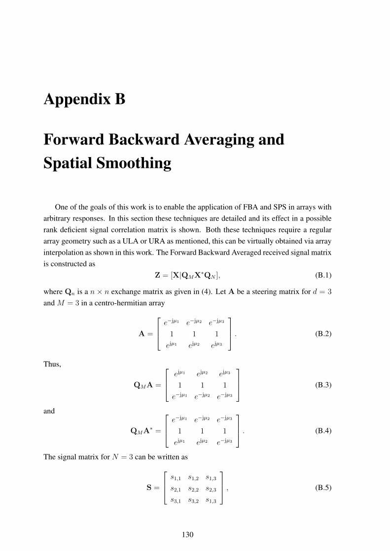
Appendix B
Forward Backward Averaging andSpatial Smoothing
One of the goals of this work is to enable the application of FBA and SPS in arrays witharbitrary responses. In this section these techniques are detailed and its effect in a possiblerank deficient signal correlation matrix is shown. Both these techniques require a regulararray geometry such as a ULA or URA as mentioned, this can be virtually obtained via arrayinterpolation as shown in this work. The Forward Backward Averaged received signal matrixis constructed as
Z = [X|QMX∗QN ], (B.1)
where Qn is a n × n exchange matrix as given in (4). Let A be a steering matrix for d = 3
and M = 3 in a centro-hermitian array
A =
e−jµ1 e−jµ2 e−jµ3
1 1 1
ejµ1 ejµ2 ejµ3
. (B.2)
Thus,
QMA =
ejµ1 ejµ2 ejµ3
1 1 1
e−jµ1 e−jµ2 e−jµ3
(B.3)
and
QMA∗ =
e−jµ1 e−jµ2 e−jµ3
1 1 1
ejµ1 ejµ2 e−jµ3
. (B.4)
The signal matrix for N = 3 can be written as
S =
s1,1 s1,2 s1,3
s2,1 s2,2 s2,3
s3,1 s3,2 s1,3
, (B.5)
130
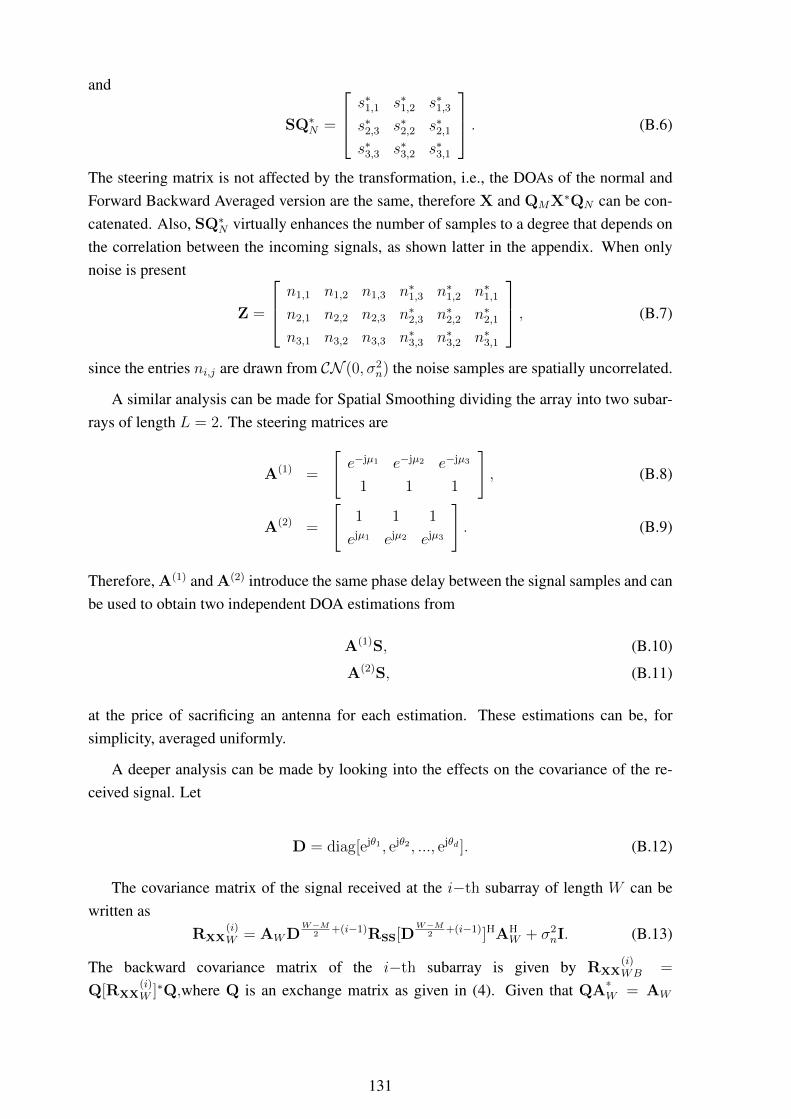
and
SQ∗N =
s∗1,1 s∗1,2 s∗1,3s∗2,3 s∗2,2 s∗2,1s∗3,3 s∗3,2 s∗3,1
. (B.6)
The steering matrix is not affected by the transformation, i.e., the DOAs of the normal andForward Backward Averaged version are the same, therefore X and QMX∗QN can be con-catenated. Also, SQ∗N virtually enhances the number of samples to a degree that depends onthe correlation between the incoming signals, as shown latter in the appendix. When onlynoise is present
Z =
n1,1 n1,2 n1,3 n∗1,3 n∗1,2 n∗1,1n2,1 n2,2 n2,3 n∗2,3 n∗2,2 n∗2,1n3,1 n3,2 n3,3 n∗3,3 n∗3,2 n∗3,1
, (B.7)
since the entries ni,j are drawn from CN (0, σ2n) the noise samples are spatially uncorrelated.
A similar analysis can be made for Spatial Smoothing dividing the array into two subar-rays of length L = 2. The steering matrices are
A(1) =
[e−jµ1 e−jµ2 e−jµ3
1 1 1
], (B.8)
A(2) =
[1 1 1
ejµ1 ejµ2 ejµ3
]. (B.9)
Therefore, A(1) and A(2) introduce the same phase delay between the signal samples and canbe used to obtain two independent DOA estimations from
A(1)S, (B.10)
A(2)S, (B.11)
at the price of sacrificing an antenna for each estimation. These estimations can be, forsimplicity, averaged uniformly.
A deeper analysis can be made by looking into the effects on the covariance of the re-ceived signal. Let
D = diag[ejθ1 , ejθ2 , ..., ejθd ]. (B.12)
The covariance matrix of the signal received at the i−th subarray of length W can bewritten as
RXX(i)W = AWD
W−M2
+(i−1)RSS[DW−M
2+(i−1)]HAH
W + σ2nI. (B.13)
The backward covariance matrix of the i−th subarray is given by RXX(i)WB =
Q[RXX(i)W ]∗Q,where Q is an exchange matrix as given in (4). Given that QA*
W = AW
131
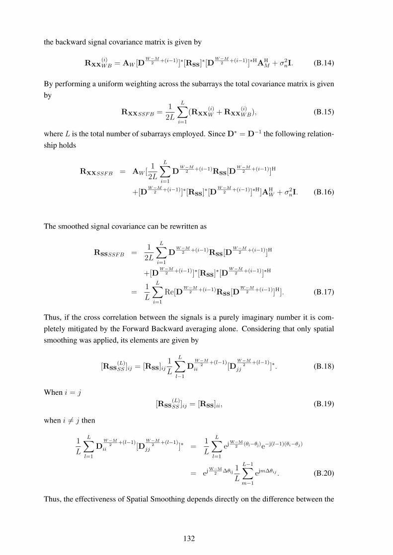
the backward signal covariance matrix is given by
RXX(i)WB = AW [D
W−M2
+(i−1)]∗[RSS]∗[DW−M
2+(i−1)]∗HAH
M + σ2nI. (B.14)
By performing a uniform weighting across the subarrays the total covariance matrix is givenby
RXXSSFB =1
2L
L∑i=1
(RXX(i)W + RXX
(i)WB), (B.15)
where L is the total number of subarrays employed. Since D∗ = D−1 the following relation-ship holds
RXXSSFB = AW [1
2L
L∑i=1
DW−M
2+(i−1)RSS[D
W−M2
+(i−1)]H
+[DW−M
2+(i−1)]∗[RSS]∗[D
W−M2
+(i−1)]∗H]AHW + σ2
nI. (B.16)
The smoothed signal covariance can be rewritten as
RSSSSFB =1
2L
L∑i=1
DW−M
2+(i−1)RSS[D
W−M2
+(i−1)]H
+[DW−M
2+(i−1)]∗[RSS]∗[D
W−M2
+(i−1)]∗H
=1
L
L∑i=1
Re[DW−M
2+(i−1)RSS[D
W−M2
+(i−1)]H]. (B.17)
Thus, if the cross correlation between the signals is a purely imaginary number it is com-pletely mitigated by the Forward Backward averaging alone. Considering that only spatialsmoothing was applied, its elements are given by
[RSS(L)SS ]ij = [RSS]ij
1
L
L∑l−1
DW−M
2+(l−1)
ii [DW−M
2+(l−1)
jj ]∗. (B.18)
When i = j
[RSS(L)SS ]ij = [RSS]ii, (B.19)
when i 6= j then
1
L
L∑l=1
DW−M
2+(l−1)
ii [DW−M
2+(l−1)
jj ]∗ =1
L
L∑l=1
ej W−M2
(θi−θj)e−j(l−1)(θi−θj)
= ej W−M2
∆θij1
L
L−1∑m−1
ejm∆θij . (B.20)
Thus, the effectiveness of Spatial Smoothing depends directly on the difference between the
132

∆θij between the angles of arrival of the signals indexed by i and j, this is why SpatialSmoothing is applied mostly in a heuristic manner and why, in this work, a simple way ofchoosing the minimum number of subarrays that provides proper signal decorrelation wasproposed.
133

Appendix C
Proof of Theorem 1
Proof. Let a random variable r have a probability distribution function pr(r), r ∈ R. As-suming that a moment generating function Mr(k) exists, it is equivalent to the two-sidedLaplace transform of r. Hence,
Mr(−k) = L{pr(r)}(k) + L{pr(−r)}(−k), (C.1)
where L{pr(r)}(k) is the Laplace transform of pr(r). Thus, Mr(−k) is unique iff both sidesof the Laplace transform are unique. Therefore, since the Laplace transform of a function isunique, so is Mr(−k). Thus, a PDF can be uniquely described by its moments provided thatall moments exist and that pr(r) is integrable on any finite subset over its support.
134

Appendix D
Proof of Theorem 2
Proof. The log-likelihood can be given as
l(X;θ,φ) = −MN log(πσ2n)
− 1
σ2n
tr{
(X−AS)− (X−AS)H}, (D.1)
where tr{.} is the trace operator. Differentiating (D.1) with respect to σ2n and equating to
zero leads an estimate for the noise variance
σ2n =
1
MNtr{
(X−AS)− (X−AS)H}. (D.2)
Substituting (D.2) into (D.1), differentiating with respect to S, and equating to zero givesan estimate for S
S = (AH A)−1AHX. (D.3)
Then, substituting (D.2) and (D.3) into (D.1) yields
(θ, φ) = arg maxθ,φ
tr{
A(AHA)−1AHRXX
}= arg max
θ,φlc(X;θ,φ). (D.4)
Assuming that the received signals have low spatial correlation with
∀di, i′ = 1
i 6= i′
aH(θi, φi)a(θi′ , φi′)→ 0, (D.5)
135
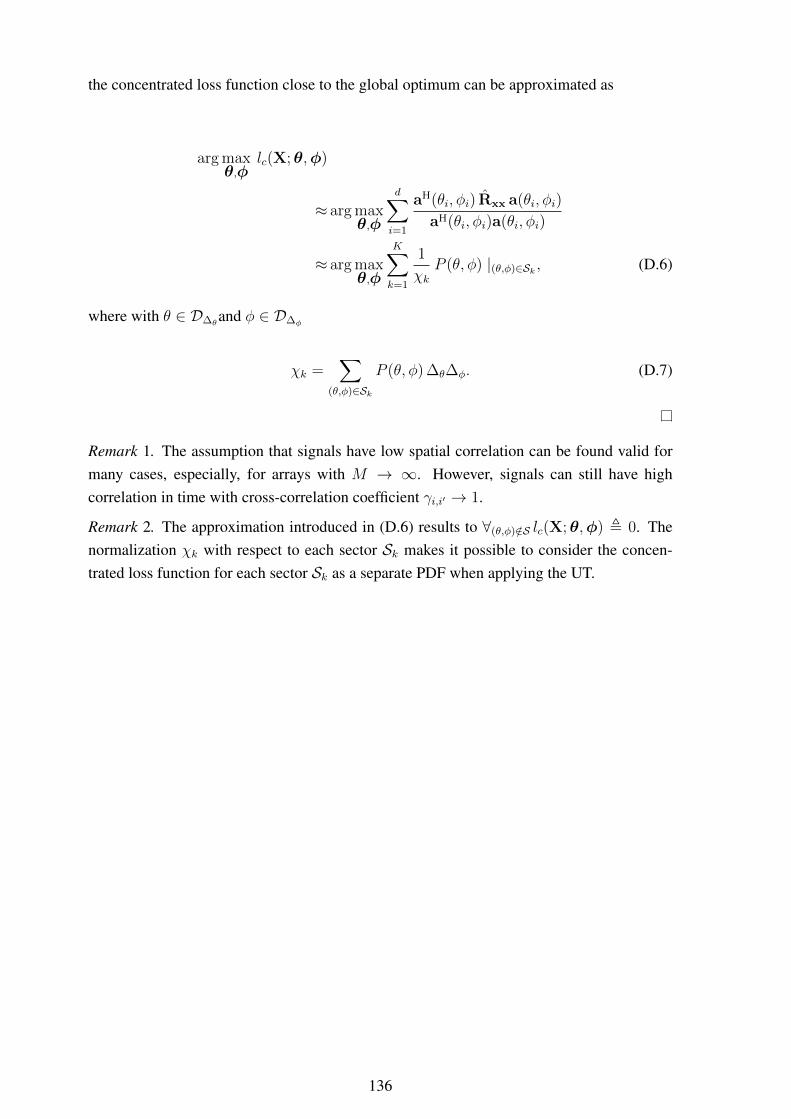
the concentrated loss function close to the global optimum can be approximated as
arg maxθ,φ
lc(X;θ,φ)
≈ arg maxθ,φ
d∑i=1
aH(θi, φi) Rxx a(θi, φi)
aH(θi, φi)a(θi, φi)
≈ arg maxθ,φ
K∑k=1
1
χkP (θ, φ) |(θ,φ)∈Sk , (D.6)
where with θ ∈ D∆θand φ ∈ D∆φ
χk =∑
(θ,φ)∈Sk
P (θ, φ) ∆θ∆φ. (D.7)
Remark 1. The assumption that signals have low spatial correlation can be found valid formany cases, especially, for arrays with M → ∞. However, signals can still have highcorrelation in time with cross-correlation coefficient γi,i′ → 1.
Remark 2. The approximation introduced in (D.6) results to ∀(θ,φ)/∈S lc(X;θ,φ) , 0. Thenormalization χk with respect to each sector Sk makes it possible to consider the concen-trated loss function for each sector Sk as a separate PDF when applying the UT.
136
Appendix E
Multivariate Adaptive Regression Splines(MARS)
The MARS [41] regression model is an extension of piece wise linear regression models.MARS uses a set of splines as basis functions, these splines in turn have the input variablesof the model as their parameters. MARS is an attractive regression technique due to the factthat it is capable of representing nonlinear relationships between input and output variablesthrough the multiplication of basis functions. MARS is also a non-parametric regressionmodel, therefore it is capable of deriving the relationship between input and output variablespurely based on the data and requires no presumptions.
The MARS model relies on basis functions known as hinge functions. Hinge functionstake the form
h(k, z) =
max(0, k − z)
or
max(0, z − k)
(E.1)
where
max(a, b) =
{a if a > b
b if a ≤ b, (E.2)
and k is known as a knot. The set C = {max(0, k − z), max(0, z − k)} is called a reflectedpair.
Let zi ∈ RI be a vector containing the observations of the I input variables belongingto the set I for a given training data observation. Let O be the total number of training dataobservations andO be the set containing all the observed values for the input variable duringtraining. The set of candidate basis functionsH for a given MARS model can be built usingall the possible combinations of the pairs max(0, k − z) and max(0, z − k) with k ∈ O andz ∈ I. Therefore,
|H| = 2IO, (E.3)
137

MARS performs two steps in order to create the model of the form
f(z) = β0 +L∑l=1
βlhl(z), (E.4)
where hl(z) ∈ H and β0, . . . , βL are weighting coefficients calculated using the normal leastsquares, and z is a vector containing the observations of the input variables. Note that despitehaving as an argument the vector with all input variables, each hl(z) is only a function of asingle element z ∈ z.
The process of building the MARS model is divided in two phases called the forward andthe backwards pass. In the forward pass, basis functions are added to the model setM inreflected pairs withM⊆ H . The basis functions from the candidate setH are added to themodel set based on their influence on the total regression error. Only once the setM has atleast one basis function, products of candidate functions and functions already present inMare also considered. Therefore, for |M| > 1 the following candidate functions are assessedusing
cmhc(z), (E.5)
where hc(z) ∈ H and cm ∈ 1 ∪M. Therefore, the model is capable of creating nonlinearrelationships by multiplying basis functions, but products of basis functions are only addedto the model if their lower order part of the product is already present on the model. Basisfunctions are added until the model reaches a given maximum model complexity νmax andbasis functions products are only considered up to a maximum order ϑmax.
After the model has reached its maximum allowed complexity, it is probably over-fitted.Thus, the second phase of the MARS model building, the backward pass, is used to reducethe model complexity. In this phase, the basis functions that are in the setM and that whenremoved impact the squared error the least, are removed. To estimate the optimal modelcomplexity, MARS uses the generalized cross-validation (GCV), which is defined as
GCV(ν) =
∑Oo=1 (yo − fν(zo))2(
1− ν+pO
)2 , (E.6)
where yi is the i-th training output, fν is a model of complexity ν and p is a penalty factor.Different values for p are discussed in [41], where a value of 3 is suggested as a default value.The GCV penalizes a model based on its complexity and creates a compromise betweenaccuracy and complexity. Maximizing the GCV reduces over-fitting and creates and moregeneral model.
138
Appendix F
Generalized Regression Neural Networks(GRNNs)
GRNNs are probabilistic neural networks, thus the number of training samples requiredis significantly reduced. Since measurements of real antenna array responses can be limitedin resolution due to the computational complexity for electromagnetic simulations or thehardware available at measurement anechoic chambers, the usage of a probabilistic neuralnetwork can be beneficial.
A GRNN relies on centering a normal distribution around the training samples accordingto
c(b) =
∑Ii=1 ci exp
(− D2
i
2σ2
)∑I
i=1 exp(− D2
i
2σ2
) , (F.1)
whereD2i = (b− bi)
T(b− bi), (F.2)
c(b) is the estimated output given the input vector b, bi is the i-th training input vector, ciis the i-th training output, σ2 is known as the smoothness parameter and is usually chosenheuristically, and i = 1, . . . , I where I is the number of training samples available.
In a GRNN the weight of a given training sample on the estimation of the output is givenby (F.2) which is the euclidean distance between a training input and the system input. AGRNN allows a small number of training samples to be used due to the fact that it is capableof interpolating between training samples using the calculated weights, as shown in (F.1).
Figure F.1 depicts how a GRNN with input vector b ∈ RJ can be built as a parallel neuralnetwork. The individual layers can have their computations performed in parallel making itpossible to speed up the application of the neural network.
139
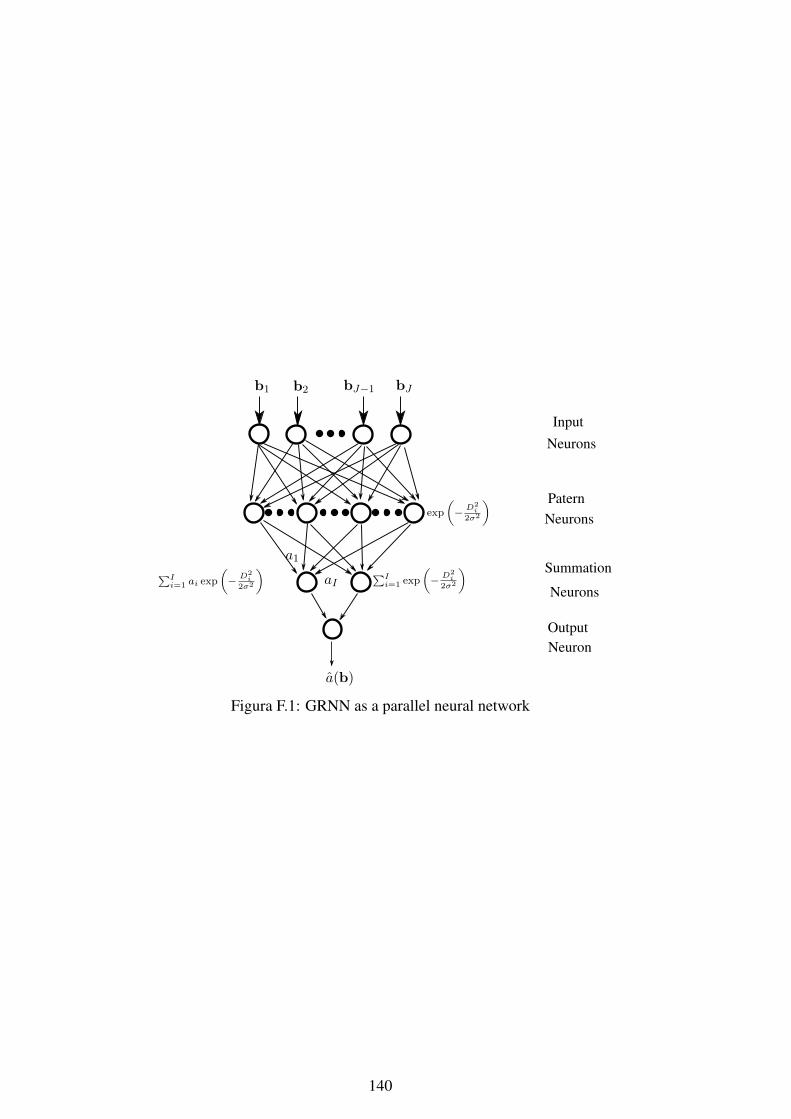
b1 b2 bJbJ−1
Input
Paternexp
(− D2
i2σ2
)
a1
aI∑Ii=1 ai exp
(− D2
i2σ2
) ∑Ii=1 exp
(− D2
i2σ2
) Summation
Output
a(b)
Neurons
Neurons
Neurons
Neuron
Figura F.1: GRNN as a parallel neural network
140
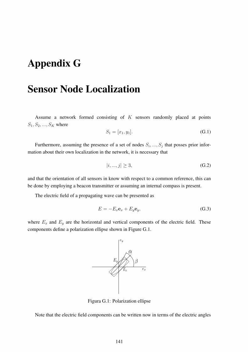
Appendix G
Sensor Node Localization
Assume a network formed consisting of K sensors randomly placed at pointsS1, S2, ..., SK where
S1 = [x1, y1]. (G.1)
Furthermore, assuming the presence of a set of nodes Si, ..., Sj that posses prior infor-mation about their own localization in the network, it is necessary that
|i, ..., j| ≥ 3, (G.2)
and that the orientation of all sensors in know with respect to a common reference, this canbe done by employing a beacon transmitter or assuming an internal compass is present.
The electric field of a propagating wave can be presented as
E = −Exex + Eyey, (G.3)
where Ex and Ey are the horizontal and vertical components of the electric field. Thesecomponents define a polarization ellipse shown in Figure G.1.
Figura G.1: Polarization ellipse
Note that the electric field components can be written now in terms of the electric angles
141

α and β as
Ex = E cos(γ) (G.4)
Ey = E sin(γ)ejη (G.5)
where
cos(2γ) = cos(2α) cos(2β) (G.6)
tan(η) = tan(2α) csc(2β). (G.7)
Considering a wavefront impinging over a crossed dipole with components parallel tothe x− and y−axis of the polarization ellipse the output at such dipoles will be proportionalto the components Ex and Ey respectively and be written as
E = (−Ex)ex + (Ey cos(θ))ey
= − cos(γ)ex + sin(γ) cos(θ)ejηey (G.8)
where θ is the angle of arrival of the received wave with respect to the x− axis.
The received signal can now be expressed in matrix as
X = us + N (G.9)
where X ∈ C2×N is the matrix containing the measured outputs at each of the dipoles, N isthe number of measured snapshots, s ∈ C1×N is the vector contain the original transmittedsignal transmitted, N ∈ C2×N is the matrix containing the Additive White Gaussian noisepresent at sampling and the vector u ∈ C2×1 is defined as
u =
[− cos(γ)
sin(γ) cos(θ)ejη
]. (G.10)
This localization approach consists of analysing the ratio between the outputs of thecrossed dipole in order to estimate the direction of arrival of the received signal. Given theratio
r =− cos(γ)
sin(γ) cos(θ)ejη, (G.11)
the angle θ can be obtained by
θ = cos−1
( − cos(γ)
r sin(γ)ejη
). (G.12)
One way to estimate the ratios is to simply average a large number of samples from bothantennas in order to reduce the effects of the noise and obtain the ratio between the powers.
142
It is important to highlight at this point that although there is a need for a crossed dipolewith two independent outputs to be present it is not necessary that both outputs are connectto individual receiver radios. A single symbol can be measured at both outputs by dividingthe symbol duration, assuming the transmitted energy is constant over the entire symbolduration.
A more precise approach is to employ the ESPRIT algorithm in order to obtain the ratiobetween the received symbols. The advantage of the ESPRIT algorithm is that it is capableof dealing much more efficiently with noise since it relies on an eigendecomposition thatseparates noise and signal subspaces.
Although the ESPRIT method is capable of obtaining more precise estimates it generatesa larger computational load. This load is, however, justified as a small error in the estimatedratio may lead to a large error in the estimation of the DOA. This computationally demandingstep is also only necessary once every time the topology of the network changes, thus, theratio at which sensors change location needs to be taken into account when choosing theestimation method.
Note that the DOA is given with respect to the reference of the x−axis and cannot dis-tinguish from with direction, front or rear, the signal is arriving. Furthermore, θ ranges from[−π, π] and thus it is also not possible to tell from with sector is the signal actually arrivingsince the only information that the system has is cos(θ). The end result is that each sensorpossesses two estimated lines in the ground plane where the transmitting node may be lo-cated. However, by acquiring a set of line estimates it is possible to obtain a single estimateof the transmitting sensor localization. The problem is reduced to the least squares problemof finding the point with minimum distance from any of the possible combination of lineestimates.
By writing the representing the line estimates as line equations of the typeAx+By+C =
0 in the sensor coordinate system, the estimate of the sensor position can be found by solving
minp
|Ap1x0 +Bp1y0 + Cp1|√Ap1 +Bp1
+|Ap2x0 +Bp2y0 + Cp2 |√
Ap2 +Bp2
+ ..., (G.13)
where p is an index set containing the possible combinations of estimated lines. Whilemore than three sensors can be used to obtain increased accuracy it also results in a highercomputational load involved in the calculation of the minima. Once the lines are choose thefinal location estimate S0 = [x0, y0] can be found by taking the derivative of the above withrespect to x0 and y0 and finding the point where it is equal to zero.
Furthermore, this technique may be used in conjunction with other localization methodssuch as the RSSI. A set of candidate locations can be selected and the RSSI information canbe used to choose the candidate that best fits the RSSI information.
143
Appendix H
TRIAD Algorithm
The TRIAD [8, 9] algorithm allowed the development of early satellite navigation sys-tems and still represents the state of practice for space and aircraft instrument based attitudeestimation. It involves only two linear independent reference vectors and their respectivemeasured directions.
By defining two linearly independent reference vectors
~R1 = [x~R1, y~R1
, z~R1]T ,
~R2 = [x~R2, y~R2
, z~R2]T , (H.1)
and their respective measured direction vectors
~r1 = [x~r1 , y~r1 , z~r1 ]T ,
~r2 = [x~r2 , y~r2 , z~r2 ]T . (H.2)
The TRIAD algorithm tries to find the rotation matrix W that satisfies
~ri = W ~Ri, (H.3)
where WTW = I and det(W) = ±1, i.e W is a orthogonal matrix and preserves themagnitude of any vector ~Ri it operates on. Since ~R1 and ~R2 are linearly independent vectors,a linear independent vector orthogonal to both can by obtained by
~R3 = ~R1 × ~R2, (H.4)
where × is the vector cross product operation, the same can be done for ~r1 and ~r2
~r3 = ~r1 × ~r2. (H.5)
Since a rotation applied to ~R1 and ~R2 would also rotate ~R3, a linear system can be written
144
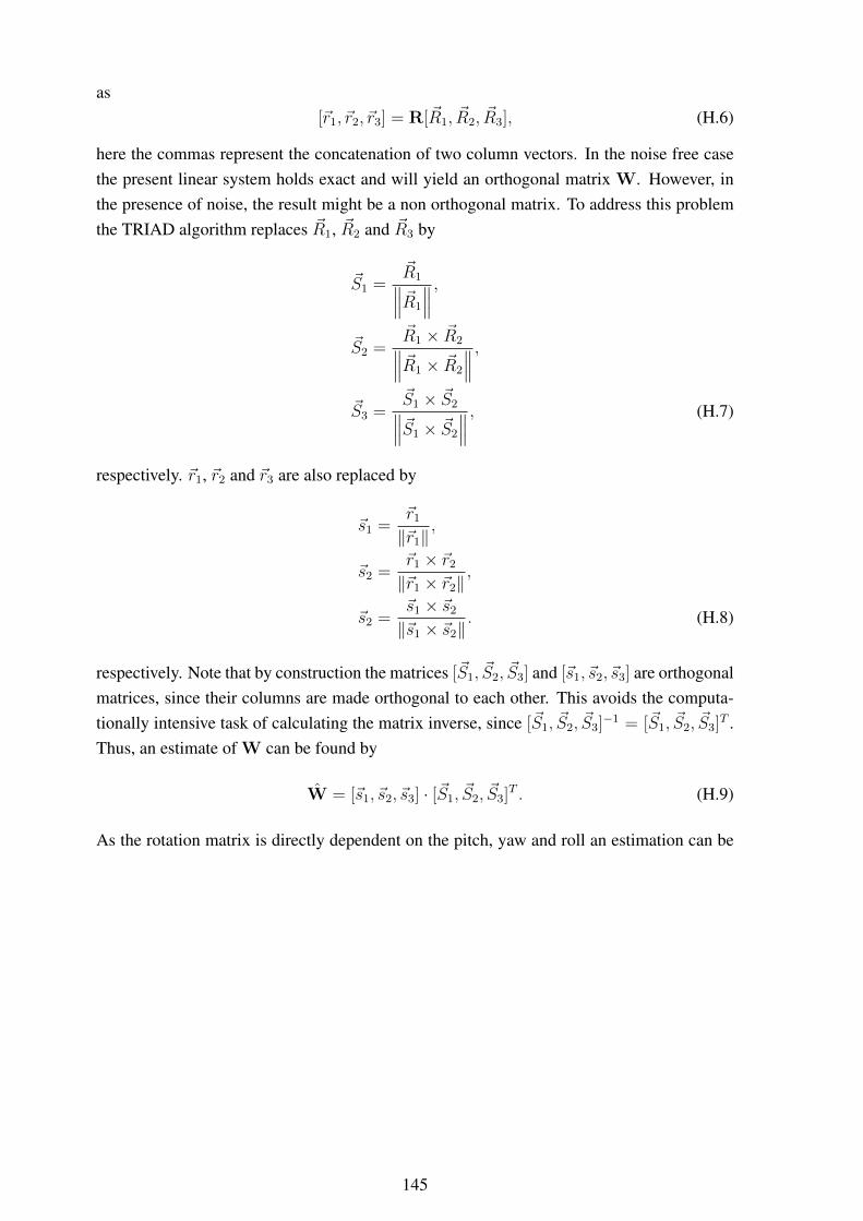
as[~r1, ~r2, ~r3] = R[~R1, ~R2, ~R3], (H.6)
here the commas represent the concatenation of two column vectors. In the noise free casethe present linear system holds exact and will yield an orthogonal matrix W. However, inthe presence of noise, the result might be a non orthogonal matrix. To address this problemthe TRIAD algorithm replaces ~R1, ~R2 and ~R3 by
~S1 =~R1∥∥∥~R1
∥∥∥ ,~S2 =
~R1 × ~R2∥∥∥~R1 × ~R2
∥∥∥ ,~S3 =
~S1 × ~S2∥∥∥~S1 × ~S2
∥∥∥ , (H.7)
respectively. ~r1, ~r2 and ~r3 are also replaced by
~s1 =~r1
‖~r1‖,
~s2 =~r1 × ~r2
‖~r1 × ~r2‖,
~s2 =~s1 × ~s2
‖~s1 × ~s2‖. (H.8)
respectively. Note that by construction the matrices [~S1, ~S2, ~S3] and [~s1, ~s2, ~s3] are orthogonalmatrices, since their columns are made orthogonal to each other. This avoids the computa-tionally intensive task of calculating the matrix inverse, since [~S1, ~S2, ~S3]−1 = [~S1, ~S2, ~S3]T .Thus, an estimate of W can be found by
W = [~s1, ~s2, ~s3] · [~S1, ~S2, ~S3]T . (H.9)
As the rotation matrix is directly dependent on the pitch, yaw and roll an estimation can be
145
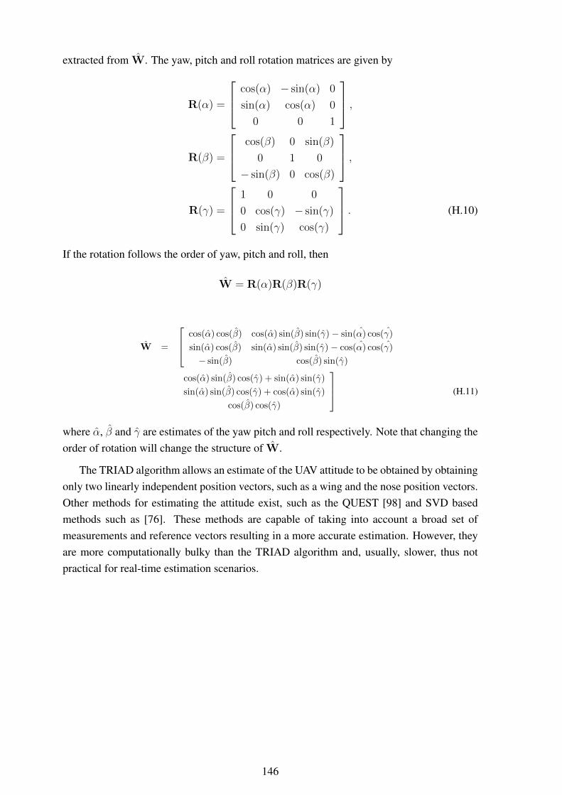
extracted from W. The yaw, pitch and roll rotation matrices are given by
R(α) =
cos(α) − sin(α) 0
sin(α) cos(α) 0
0 0 1
,
R(β) =
cos(β) 0 sin(β)
0 1 0
− sin(β) 0 cos(β)
,
R(γ) =
1 0 0
0 cos(γ) − sin(γ)
0 sin(γ) cos(γ)
. (H.10)
If the rotation follows the order of yaw, pitch and roll, then
W = R(α)R(β)R(γ)
W =
cos(α) cos(β) cos(α) sin(β) sin(γ)− sin(α) cos(γ)
sin(α) cos(β) sin(α) sin(β) sin(γ)− cos(α) cos(γ)
− sin(β) cos(β) sin(γ)
cos(α) sin(β) cos(γ) + sin(α) sin(γ)
sin(α) sin(β) cos(γ) + cos(α) sin(γ)
cos(β) cos(γ)
(H.11)
where α, β and γ are estimates of the yaw pitch and roll respectively. Note that changing theorder of rotation will change the structure of W.
The TRIAD algorithm allows an estimate of the UAV attitude to be obtained by obtainingonly two linearly independent position vectors, such as a wing and the nose position vectors.Other methods for estimating the attitude exist, such as the QUEST [98] and SVD basedmethods such as [76]. These methods are capable of taking into account a broad set ofmeasurements and reference vectors resulting in a more accurate estimation. However, theyare more computationally bulky than the TRIAD algorithm and, usually, slower, thus notpractical for real-time estimation scenarios.
146


![Sparse Array Antenna Signal Reconstruction using ... · ix List of symbols Symbol Description a(𝜃) [Nx1] array steering vector corresponding to the direction 𝜃. AF Array Factor](https://static.fdocuments.us/doc/165x107/5f80b5457d4c0167d10cada0/sparse-array-antenna-signal-reconstruction-using-ix-list-of-symbols-symbol-description.jpg)