Array Processing Techniques forDirection of Arrival Estimation,Communications, and Localization inVehicular and Wireless Sensor Networks

Marco Antonio Marques Marinho

D O C T O R A L T H E S I S | Halmstad University Dissertations no. 43

Supervisors: Alexey VinelJoão Paulo Carvalho Lustosa da CostaFelix Antreich

Array Processing Techniques for Direction of Arrival Estimation, Communications, and Localization in Vehicular and Wireless Sensor Networks© Marco Antonio Marques MarinhoHalmstad University Dissertations no. 43 ISBN 978-91-87045-88-2 (printed)ISBN 978-91-87045-89-9 (pdf)Publisher: Halmstad University Press, 2018 | www.hh.se/hup

Aos meus pais:Marco Antonio e Marcelita, tudo que há de bom em mim nasceu devocês. Aprendi muito ao longo desses anos de doutorado longe de vocês,mas a maior lição que aprendi é vocês são as pessoas mais importantesda minha vida. Amo vocês acima de tudo.

Ao meu irmão:Murilo, companheiro ao longo dessa jornada que escolhemos. Sem nos-sas conversas e discussões sobre a vida de um doutorando eu provavel-mente teria perdido a batalha mais importante dessa guerra, a demater-me são e sensato. Obrigado por tudo.

A minha noiva:Stephanie, minha parceira e amiga. A distância ao longo desses anosnão foi capaz de diminuir seu amor, companheirismo e carinho. Obri-gado por sua dedicação e paciência nos momentos mais difíceis. Suaforça em frente as di�culdades foi uma grande fonte de inspiração. Teamo.

Marco Antonio Marques Marinho

i

Abstract

Array signal processing in wireless communication has been a topic of inter-est in research for over three decades. In the fourth generation (4G) of thewireless communication systems, also known as Long Term Evolution (LTE),multi antenna systems have been adopted according to the Release 9 of the3rd Generation Partnership Project (3GPP). For the �fth generation (5G) ofthe wireless communication systems, hundreds of antennas should be incorpo-rated to the devices in a massive multi-user Multiple Input Multiple Output(MIMO) architecture. The presence of multiple antennas provides array gain,diversity gain, spatial gain, and interference reduction. Furthermore, arrays en-able spatial �ltering and parameter estimation, which can be used to help solveproblems that could not previously be addressed from a signal processing per-spective. The aim of this thesis is to bridge some gaps between signal processingtheory and real world applications. Array processing techniques traditionallyassume an ideal array. Therefore, in order to exploit such techniques, a robustset of methods for array interpolation are fundamental and are developed inthis work. In this dissertation, novel methods for array interpolation are pre-sented and their performance in real world scenarios is evaluated. Problems inthe �eld of wireless sensor networks and vehicular networks are also addressedfrom an array signal processing perspective. Signal processing concepts are im-plemented in the context of a wireless sensor network. These concepts providea level of synchronization su�cient for distributed multi antenna communica-tion to be applied, resulting in improved lifetime and improved overall networkbehaviour. Array signal processing methods are proposed to solve the problemof radio based localization in vehicular network scenarios with applications inroad safety and pedestrian protection.

iii

Acknowledgments

To Prof. Felix Antreich, my friend, mentor, and co-supervisor. For helpingme out through the rough patches along the way, not just academically, butalso when got the short end of the stick after physical encounters with motorvehicles. Without his support and guidance I would not have arrived at thisdestination. It is a great honor to work and research alongside him.

To my supervisor Prof. João Paulo Carvalho Lustosa da Costa, to whom Iown so much, for the endless support throughout my entire academic career.I am thankful for his patience, trust and for the endless opportunities he hasprovided me during my academic career. It is thanks to him I have gotten toexperience so much of the world and had the opportunity to know so manyinteresting �elds of research.

To my supervisor Prof. Alexey Vinel, who deposited so much trust in meby accepting me as a student in Halmstad. He always did his best and dedi-cated so much time to ensure I could apply my knowledge to interesting andrelevant topics during my stay in Sweden. I appreciate all his e�ort to makemy Ph.D. experience productive and stimulating. Without his help many in-teresting results would never have come to be.

To Prof. Edison Pignaton de Freitas for his support and incentive acrossmy academic career. He was always able to keep a good humour even when Ihad lost mine. His seamlessly endless ability to moderate con�ict and connectpeople have help me throughout this journey and serve as a great inspiration.

To Prof. Fredrik Tufvesson for the time dedicated to following my workand for all the suggestions and guidance o�ered.

v

Contents

Introduction 1

1 Array Interpolation 51.1 Overview and Contribution . . . . . . . . . . . . . . . . . . . . 51.2 Motivation . . . . . . . . . . . . . . . . . . . . . . . . . . . . . 71.3 Data Model . . . . . . . . . . . . . . . . . . . . . . . . . . . . . 111.4 Preliminaries . . . . . . . . . . . . . . . . . . . . . . . . . . . . 13

1.4.1 Forward Backward Averaging (FBA) . . . . . . . . . . . 131.4.2 Spatial Smoothing (SPS) . . . . . . . . . . . . . . . . . 141.4.3 Model Order Selection . . . . . . . . . . . . . . . . . . 141.4.4 Estimation of Signal Parameters via Rotational Invari-

ance Techniques (ESPRIT) . . . . . . . . . . . . . . . . 151.4.5 Vandermonde Invariance Transformation (VIT) . . . . 17

1.5 Array Interpolation . . . . . . . . . . . . . . . . . . . . . . . . . 181.6 Classical Interpolation . . . . . . . . . . . . . . . . . . . . . . . 191.7 Sector Selection and Discretization . . . . . . . . . . . . . . . . 23

1.7.1 UT Discretization . . . . . . . . . . . . . . . . . . . . . 261.7.2 Principal Component Discretization . . . . . . . . . . . 28

1.8 Linear Adaptive Array Interpolation . . . . . . . . . . . . . . . 291.8.1 Data Transformation and Model Order Selection . . . . 321.8.2 Linear UT Array Interpolation . . . . . . . . . . . . . . 34

1.9 Multidimensional Linear Interpolation . . . . . . . . . . . . . . 351.9.1 Tensor Algebra Concepts . . . . . . . . . . . . . . . . . 351.9.2 Multidimensional Data Model . . . . . . . . . . . . . . . 361.9.3 Multidimensional Interpolation . . . . . . . . . . . . . . 37

1.10 Nonlinear Array Interpolation . . . . . . . . . . . . . . . . . . . 381.10.1 MARS based interpolation . . . . . . . . . . . . . . . . 391.10.2 GRNN based interpolation . . . . . . . . . . . . . . . . 40

1.11 Numerical Simulation Results . . . . . . . . . . . . . . . . . . . 411.11.1 Multidimensional Linear Performance Results . . . . . . 411.11.2 Nonlinear Performance Results . . . . . . . . . . . . . . 44

1.12 Summary . . . . . . . . . . . . . . . . . . . . . . . . . . . . . . 49

vii

2 Cooperative MIMO for Wireless Sensor Networks 512.1 Overview and Contribution . . . . . . . . . . . . . . . . . . . . 512.2 Motivation . . . . . . . . . . . . . . . . . . . . . . . . . . . . . 522.3 Wireless Sensor Networks Organization . . . . . . . . . . . . . 542.4 Cooperative MIMO . . . . . . . . . . . . . . . . . . . . . . . . . 552.5 Energy Analysis . . . . . . . . . . . . . . . . . . . . . . . . . . 58

2.5.1 Conventional Techniques . . . . . . . . . . . . . . . . . . 592.5.2 Cooperative MIMO . . . . . . . . . . . . . . . . . . . . 61

2.6 Synchronization . . . . . . . . . . . . . . . . . . . . . . . . . . . 642.6.1 E�ects of Synchronization Error on Cooperative MIMO 642.6.2 Proposed Coarse Synchronization Scheme . . . . . . . . 652.6.3 Proposed Fine Synchronization Schemes . . . . . . . . . 662.6.4 Synchronization error propagation . . . . . . . . . . . . 70

2.7 Adaptive C-MIMO Clustering . . . . . . . . . . . . . . . . . . 732.7.1 Adaptive C-MIMO clustering . . . . . . . . . . . . . . . 742.7.2 Numerical Simulations . . . . . . . . . . . . . . . . . . . 78

2.8 Summary . . . . . . . . . . . . . . . . . . . . . . . . . . . . . . 85

3 Array Processing Localization for Vehicular Networks 873.1 Overview and Contribution . . . . . . . . . . . . . . . . . . . . 873.2 Motivation . . . . . . . . . . . . . . . . . . . . . . . . . . . . . 883.3 Data Model . . . . . . . . . . . . . . . . . . . . . . . . . . . . . 903.4 Space-Alternating Generalized Expectation Maximization (SAGE)

Algorithm . . . . . . . . . . . . . . . . . . . . . . . . . . . . . . 913.5 Scenario Description . . . . . . . . . . . . . . . . . . . . . . . . 923.6 Array Processing Localization . . . . . . . . . . . . . . . . . . . 93

3.6.1 Flip-Flop Estimation . . . . . . . . . . . . . . . . . . . 933.6.2 Joint Direct Position Estimation . . . . . . . . . . . . . 963.6.3 DOA only estimation . . . . . . . . . . . . . . . . . . . 973.6.4 Applicability of DOA Estimation for Positioning . . . . 98

3.7 Three Dimensional DOA Based Estimation . . . . . . . . . . . 993.7.1 Scenario Description . . . . . . . . . . . . . . . . . . . . 993.7.2 De�nition of the Attitude Angles . . . . . . . . . . . . . 993.7.3 Direction vector computation . . . . . . . . . . . . . . . 1003.7.4 Position estimation . . . . . . . . . . . . . . . . . . . . 100

3.8 Simulation Results . . . . . . . . . . . . . . . . . . . . . . . . . 1013.8.1 Results for Simulated Data . . . . . . . . . . . . . . . . 1013.8.2 Results for Real Data . . . . . . . . . . . . . . . . . . . 104

3.9 Summary . . . . . . . . . . . . . . . . . . . . . . . . . . . . . . 107

Conclusion 109

Author's Publications 113

References 117

viii

Appendices 131A Left Centro-Hermitian Matrix . . . . . . . . . . . . . . . . . . 133B Forward Backward Averaging and Spatial Smoothing . . . . . 135C Proof of Theorem 1 . . . . . . . . . . . . . . . . . . . . . . . . 139D Proof of Theorem 2 . . . . . . . . . . . . . . . . . . . . . . . . 141E Multivariate Adaptive Regression Splines (MARS) . . . . . . . 143F Generalized Regression Neural Networks (GRNNs) . . . . . . . 145G Sensor Node Localization . . . . . . . . . . . . . . . . . . . . . 147H TRIAD Algorithm . . . . . . . . . . . . . . . . . . . . . . . . . 151

ix

List of Figures

1.1 Signal with DOA θ impinging on a uniform linear array (ULA),whose the antenna space is ∆ . . . . . . . . . . . . . . . . . . 8

1.2 On the left side there is real data from an antenna array, whileon the right side the data transformed by the transformationmatrix B . . . . . . . . . . . . . . . . . . . . . . . . . . . . . . 9

1.3 Graphical representation of a linear array . . . . . . . . . . . . 121.4 Example of SPS subarrays . . . . . . . . . . . . . . . . . . . . . 141.5 Eigenvalue pro�le: eigenvalue index versus eingenvalue . . . . . 151.6 P (θ, φ) . . . . . . . . . . . . . . . . . . . . . . . . . . . . . . . . 241.7 Selected sectors and example of sector bounds . . . . . . . . . . 251.8 Selected sectors and respective bounds for one-dimensional case 261.9 UT of the approximated lc(X;θ,φ) for two sources . . . . . . . 281.10 Example of transformed regions . . . . . . . . . . . . . . . . . . 301.11 Transformation error with respect to combined sector size . . . 311.12 Example of estimated model order versus number of subarrays 331.13 Tensor B ∈ R2×2×2 . . . . . . . . . . . . . . . . . . . . . . . . . 351.14 Results for a standard deviation of π

20 radians . . . . . . . . . . 421.15 Results for a standard deviation of π

10 radians . . . . . . . . . . 431.16 Results for a standard deviation of π5 radians . . . . . . . . . . 431.17 6x1 antenna array: ANSYS HFSS model (left), prototype (right).

. . . . . . . . . . . . . . . . . . . . . . . . . . . . . . . . . . . . 451.18 DOA estimation performance with 0.4 λ element separation . . 461.19 DOA estimation performance with 0.2 λ element separation . . 461.20 DOA estimation performance for model built with simulated

data with 0.4 λ element separation . . . . . . . . . . . . . . . . 471.21 DOA estimation performance for model built with simulated

data with 0.2 λ element separation . . . . . . . . . . . . . . . . 481.22 TLS-ESPRIT failure rate for 0.2 λ element separation . . . . . 48

2.1 Examples of peer-to-peer and cluster networks . . . . . . . . . 552.2 Example of cooperative MIMO and SISO communications in a

wireless sensor network . . . . . . . . . . . . . . . . . . . . . . . 562.3 C-MIMO communication steps . . . . . . . . . . . . . . . . . . 56

xi

2.4 Performance comparison between standard SISO systems and2× 2 MIMO systems using ZF, MMSE and ML equalization . . 58

2.5 Examples of single-hop and multi-hop communication . . . . . 592.6 Performance comparison of equalization methods in the pres-

ence of synchronization errors in a 2x2 MIMO system . . . . . 652.7 Performance comparison of equalization methods in the pres-

ence of synchronization errors in a 4x4 MIMO system . . . . . 662.8 Performance comparison of equalization methods in the pres-

ence of synchronization errors in a 7x7 MIMO system . . . . . 672.9 Performance of ML synchronization,

f =20 MHz, B = 22 MHz . . . . . . . . . . . . . . . . . . . . . 692.10 Performance of proposed DFT based synchronization, f =20

MHz, B = 22 MHz . . . . . . . . . . . . . . . . . . . . . . . . . 702.11 Histogram of synchronization error using the MLmethod (2.22,2.24) 712.12 Histogram of synchronization error using the DFT method (2.25) 712.13 Comparison of individual node energy depletion using C-MIMO

or multihop only . . . . . . . . . . . . . . . . . . . . . . . . . . 802.14 Comparison of individual node energy depletion using multihop

only after 2500 seconds . . . . . . . . . . . . . . . . . . . . . . . 822.15 Comparison of individual node energy depletion using C-MIMO

after 2500 seconds . . . . . . . . . . . . . . . . . . . . . . . . . 822.16 Comparison of individual node energy depletion using multihop

only after 4500 seconds . . . . . . . . . . . . . . . . . . . . . . . 822.17 Comparison of individual node energy depletion using C-MIMO

after 4500 seconds . . . . . . . . . . . . . . . . . . . . . . . . . 822.18 Comparison of individual node energy depletion using multihop

only after 5500 seconds . . . . . . . . . . . . . . . . . . . . . . . 822.19 Comparison of individual node energy depletion using C-MIMO

after 5500 seconds . . . . . . . . . . . . . . . . . . . . . . . . . 822.20 Example of WSN areas with di�erent energetic demands . . . 832.21 Mean available energy at the center region of the network . . . 832.22 Mean available energy at the edges of the network . . . . . . . 842.23 Standard deviation of available energy at the center region of

the network . . . . . . . . . . . . . . . . . . . . . . . . . . . . . 842.24 Standard deviation of available energy at the edges of the network 85

3.1 Scenario description for two vehicles . . . . . . . . . . . . . . . 933.2 Block diagram for the proposed �ip-�op method . . . . . . . . 953.3 System model composed of a URA at the base station and an

antenna array at the UAV. . . . . . . . . . . . . . . . . . . . . 993.4 De�nitions of pitch α, yaw β and roll γ . . . . . . . . . . . . . 1003.5 Position estimation error vs SNR . . . . . . . . . . . . . . . . . 1023.6 Position estimation error vs distance from source . . . . . . . . 1033.7 Position estimation error vs number of NLOS components . . . 1043.8 Position estimation error vs K-factor . . . . . . . . . . . . . . . 104

xii

3.9 Position estimation error over the x- and y-axes . . . . . . . . . 1053.10 Antenna array and an overview of its placement . . . . . . . . . 1053.11 Patio where measurements were performed and map of user

distribution . . . . . . . . . . . . . . . . . . . . . . . . . . . . . 1063.12 Position estimation error for measured data using the proposed

joint estimation . . . . . . . . . . . . . . . . . . . . . . . . . . . 1073.13 Position estimation error for measured data using the proposed

�ip-�op estimation . . . . . . . . . . . . . . . . . . . . . . . . . 107

F.1 GRNN as a parallel neural network . . . . . . . . . . . . . . . . 146

G.1 Polarization ellipse . . . . . . . . . . . . . . . . . . . . . . . . . 147

xiii

List of Tables

1.1 Summary of DOA estimation methods, dividing into three fam-ilies: maximum likelihood (ML), beamformers, and subspacemethods . . . . . . . . . . . . . . . . . . . . . . . . . . . . . . . 9

2.1 Energy consumption for the Mica2 platform . . . . . . . . . . . 602.2 Transmission energy consumption . . . . . . . . . . . . . . . . . 642.3 Total network energy consumption . . . . . . . . . . . . . . . . 792.4 Undeliverable packets . . . . . . . . . . . . . . . . . . . . . . . 79

xv

Introduction

This work aims to make possible the application of signal processing tech-niques in scenarios that were previously unsuitable for it. To this end, thetopic of array interpolation is addressed, allowing imperfect arrays to be usedfor array processing. Furthermore, in this dissertation, array signal processingtechniques are proposed for wireless sensor networks and vehicular networks.

The following research questions are addressed in this work:

1. How to estimate the directions of arrival of correlated sources that areimpinging on an antenna array that does not possess the necessary char-acteristics (geometry or electromagnetic response) for doing so?

2. Can array processing techniques be used to provide improved lifetimeand communication performance in wireless sensor network?

3. Can array processing techniques be used to reliably estimate positionof vehicles and pedestrians in vehicular scenarios based on their radiotransmissions?

While the overall goal of this thesis is to apply array processing to prac-tical scenarios, to allow the reader more freedom each research question isdiscussed on an individual chapter. Each chapter is presented as self-containedas possible. Therefore, the reader may read Chapter 1, Chapter 2, Chapter 3independently. At the beginning of each chapter an overview, listing the con-tents of the chapter to allow the reader to skip to sections of interest. Togetherwith the overview, a detailed list of the contributions is presented. Further-more, each chapter is given its own section providing a brief summary of thediscussion contained within, presented in Section 1.12, Section 2.8, and Section3.9, respectively.

The �rst question is addressed in Chapter 1, where robust array inter-polation methods are proposed. By applying array interpolation, data witharbitrary geometries or responses can be transformed into a tractable math-ematical model. The problem of interpolation is addressed from the groundup, and problems, such as the array discretization, are tackled. Linear andnonlinear interpolation approaches are shown, providing a wide spectrum ofalternatives that can be used according to the desired accuracy and compu-tational complexity of the application. By using numerical simulations and

1

measurements, this work shows that the proposed methods outperform thestate-of-the-art approaches. Section 1.2 presents a detailed background, andmotivation on array interpolation. The six major contributions presented isthis chapter are:

1. A signal adaptive approach for sector detection. Avoiding the pitfalls ofhaving to deal with multiple sectors or the bias introduced by transform-ing the entire �eld of view of the array.

2. Two well de�ned methods for sector discretization aiming to preservethe statistical integrity of the transformed regions while minimizing thedimensionality of the data.

3. A linear approach for interpolation that aims to maximize the trans-formed signal regions while minimizing the transformation error, mini-mizing the parameter estimation bias.

4. A nonlinear extension for the linear approach, allowing the applicationof the proposed linear method to arrays with an arbitrary number ofdimensions.

5. Two nonlinear array interpolation methods. The nonlinear approachesare suitable for dealing with arrays with highly distorted responses orimproper geometries.

6. The performance of the proposed methods is tested using real antennameasurements, validating the proposed methods under real scenarios.

Chapter 2 deals with the second research question. The developed array in-terpolation tools can be employed to distributed antenna systems, such as wire-less sensor networks (WSNs). While interpolated clusters can perform beam-forming and detect radio signal sources, a more critical problem in WSNs is theenergy e�ciency, specially with respect to communication. Another antennaarray technique, the multiple-input multiple-output (MIMO) communicationtechnique can be used to achieve improved energy e�ciency. However, to thisend, it is necessary to achieve a very high degree of synchronization. The prob-lem of synchronization is tackled, and its e�ects on the performance of MIMOsystems are assessed in detail. The energy performance of distributed MIMOsystems is analysed, and a threshold for its application is derived. The energeticperformance of a network employing cooperative MIMO is shown considerablyoutperforms state-of-the-art single-hop and multi-hop methods. A detailed in-troduction on the topic of cooperative MIMO in WSNs is presented in Section2.2. The �ve major contributions presented is this chapter are:

1. A study on the energy e�ciency of C-MIMO with respect to multi andsingle-hop communications, de�ning a threshold of selection between themultiple communication techniques.

2

2. An analysis on the impact of synchronization errors in distributed MIMOsystem with respect to the symbol period and the size of the communi-cation clusters involved.

3. A study on the propagation of synchronization errors inside a WSN,and from that the derivation of a closed form expression regarding theresynchronization interval in distributed MIMO systems that takes intoaccount the symbol duration and the clock drift of the nodes involved.

4. Two methods for synchronization for WSNs with di�erent trade-o�s be-tween performance and computational complexity.

5. An adaptive method for selecting the cluster size of C-MIMO transmis-sions capable of maximizing energy e�ciency and improve the homo-geneity of the energy reserves across the network.

The third question is studied in Chapter 3, where the problem of localiza-tion in the context of vehicular networks is tackled. A broadband data modelconsidering the spherical curvature of the received wavefront is presented. Thisdata model is leveraged to allow the estimation of the position of a transmit-ter using two separate antenna arrays. The problem is parametrized to allowthe direct estimation of the coordinates of a transmitter by jointly processingdata from both subarrays. Alternative localization approaches with reducedcomputational load based on estimating the DOA and range of a transmit-ter are also proposed. By using numerical simulations and measurements, thiswork shows that the proposed methods outperform the state-of-the-art ap-proaches, achieving a sub-meter accuracy under certain conditions. A detailedintroduction to the problem of localization in vehicular scenarios can be foundin Section 3.2, while Section 3.1 presents an overview of the chapter and itsresearch contributions. The four major contributions presented is this chapterare:

1. A DOA only localization method capable of localizing transmitters nearto a vehicle at a low computational cost.

2. A localization method based on range and DOA estimations performedat independent subarrays. The geometrical relationship between the in-dividual estimates is used to speed up the rate of convergence of theSAGE algorithm on the individual subarrays.

3. A novel parametrization for the received waveform data model allowingjoint localization estimation to be performed at both subarrays simulta-neously.

4. Localization methods that do not require the transmission of speci�clocation data that can be used to mitigate spoo�ng attacks in VANETs.

3

Chapter 1

Array Interpolation

In this chapter the following research question is addressed:How to estimate the directions of arrival of correlated sources that are imping-ing on an antenna array that does not possess the necessary characteristics(geometry or electromagnetic response) for doing so?

1.1 Overview and Contribution

The remainder of this section is organized as follows:

� Motivation: The problem of direction of arrival estimation is discussedand a detailed introduction on the subject of array interpolation pre-sented along with the challenges this work aims to tackle.

� Data Model: The spatial data model of a signal received at an antennaarray is de�ned.

� Preliminaries: Here important concepts (spatial smoothing, forwardbackward average, Vandermonde invariant transformation, model orderselection, and Estimation of Signal Parameters via Rotational InvarianceTechniques) used throughout the remainder of this chapter are presentedin detail.

� Array Interpolation: The problem of array interpolation is de�nedand a distinction between linear and nonlinear interpolation is made.

� Classical Interpolation: Here the prior methods available in the liter-ature for array interpolation are brie�y detailed.

� Sector Detection and Discretization: A signal adaptive approachthat allows sectors of interest to be detected based on the received sig-nal power is presented. Furthermore, the problem of discretizing these

5

sectors is addressed with two di�erent approaches introduced, employingthe unscented transform (UT) and principal component analysis (PCA)receptively.

� Linear Interpolation: This section presents a linear interpolation ap-proach that aims to minimize the transformation bias while transformingas much as possible of the received signal. A calculation of a transformmatrix employing the UTs parameters is discussed. The problem of se-lecting the proper smoothing length for proper signal decorrelation isdiscussed.

� Multidimensional Interpolation: Here, a multidimensional extensionof the linear approach is presented. To derive this extension a multidi-mensional data model is presented and important tensor algebra conceptsare detailed.

� Nonlinear Interpolation: This section presents two approaches forperforming array interpolation in a nonlinear fashion. A general regres-sion neural network (GRNN) and a multivariate adaptive regressionsplines (MARS) based approach are detailed.

� Simulation Results: Finally, the performance of the proposed methodsis shown by means of numerical simulations. A set of such simulationsis performed using a real measured response from an antenna array inorder to validate the proposed methods using real data.

The research contributions presented in this chapter are:

1. A signal adaptive approach for sector detection. Avoiding the pitfalls ofhaving to deal with multiple sectors or the bias introduced by transform-ing the entire �eld of view of the array.

2. Two well de�ned methods for sector discretization aiming to preservethe statistical integrity of the transformed regions while minimizing thedimensionality of the data.

3. A linear approach for interpolation that aims to maximize the trans-formed signal regions while minimizing the transformation error, mini-mizing the parameter estimation bias.

4. A nonlinear extension for the linear approach, allowing the applicationof the proposed linear method to arrays with an arbitrary number ofdimensions.

5. Two nonlinear array interpolation methods. The nonlinear approachesare suitable for dealing with arrays with highly distorted responses orimproper geometries.

6. The performance of the proposed methods is tested using real antennameasurements, validating the proposed methods under real scenarios.

6

1.2 Motivation

Sensor arrays have been applied in various �elds of modern electrical engi-neering [59]. From up and coming applications such as massive Multiple InputMultiple Output (MIMO) [62] to microphone arrays capable, for instance, ofdetecting and separating multiple sound sources or playing individual songsdepending on the seat of a car [105]. The mathematical tools provided by arraysignal processing together with the evolution of electronic circuitry have madesuch applications a reality. The problem of parameter estimation is of majorinterest in the �eld of array signal processing. Among the parameters thatcan be estimated, the direction of arrival (DOA) of an electromagnetic wavereceived at the array has experienced signi�cant attention. The parameters tobe estimated are those related to the received wave signals, spatial parameterssuch as direction of arrival (DOA) and direction of departure (DOD), tem-poral parameters such as time delay of arrival (TDOA). Moreover, frequencyparameters such as Doppler shift can be estimated by fusing together the datareceived at various antennas and using a preexisting knowledge such as thegeometry in which the antennas are organized and their responses to signalsarriving with di�erent center frequencies or from di�erent directions.

Among the parameters that can be estimated, the DOA has received par-ticular interest. Once one has knowledge of the DOAs of the received signalthe received signals may be spatially �ltered, i.e., the desired signal with aknown DOA can be e�ectively separated from signals with other direction byusing beamforming techniques. This spatial �ltering is analogous to bandpass�ltering in time domain. The DOAs are also one of the main parameters of ra-dio detection and ranging (RADAR) systems as the one proposed as a preciseradio altimeter in [53] and are specially crucial in electronic warfare.

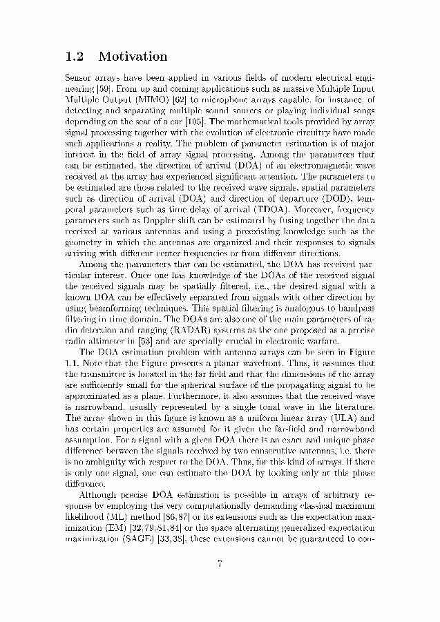
The DOA estimation problem with antenna arrays can be seen in Figure1.1. Note that the Figure presents a planar wavefront. Thus, it assumes thatthe transmitter is located in the far-�eld and that the dimensions of the arrayare su�ciently small for the spherical surface of the propagating signal to beapproximated as a plane. Furthermore, it also assumes that the received waveis narrowband, usually represented by a single tonal wave in the literature.The array shown in this �gure is known as a uniform linear array (ULA) andhas certain properties are assumed for it given the far-�eld and narrowbandassumption. For a signal with a given DOA there is an exact and unique phasedi�erence between the signals received by two consecutive antennas, i.e, thereis no ambiguity with respect to the DOA. Thus, for this kind of arrays, if thereis only one signal, one can estimate the DOA by looking only at this phasedi�erence.

Although precise DOA estimation is possible in arrays of arbitrary re-sponse by employing the very computationally demanding classical maximumlikelihood (ML) method [86,87] or its extensions such as the expectation max-imization (EM) [32,79,81,84] or the space alternating generalized expectationmaximization (SAGE) [33,38], these extensions cannot be guaranteed to con-

7

Y

. . .

Δ Δ Δ

θ

Inco

min

g Sig

nal

Figure 1.1: Signal with DOA θ impinging on a uniform linear array (ULA),whose the antenna space is ∆

verge to its local maxima, requiring a good initialization of the parameters,and can be very computationally demanding as the number of wavefrontswith parameters to be estimated can be quite high [19]. Another alternativefor DOA estimation in arbitrary array geometries is the conventional beam-former [4], this method requires a peak search and cannot properly separateclosely spaced wavefronts unless a very large number of antennas is presentat the array. An improvement over the conventional beamformer is the Caponminimum variance distortionless response (Capon-MVDR) [16]. This methodo�ers increased resolution when compared with the traditional beamformer butsu�ers in the presence of highly correlated wavefronts scenarios and requiresa peak search. The Multiple SIgnal Classi�cation (MUSIC) [95] algorithm is asubspace based algorithm that can be applied with arrays of arbitrary responseand also requires a peak search.

In contrast to ML and peak search based methods, there are also, in theliterature, a vast number of algorithms that are either closed-form or requirevery few iterations. Examples of such techniques are the Iterative QuadraticMaximum Likelihood (IQML) [10], Root Weighted Subspace Fitting (Root-WSF) [101] and Root-MUSIC [3] methods. However, all of these methodsrely on a Vandermonde or left centro-hermitian array response. Left centro-hermitian matrices are de�ned in Appendix A. Spatial Smoothing (SPS) [37]and Forward Backward Averaging (FBA) [90] also require Vandermonde andcentro-hermitian array responses, respectively. These techniques enable theapplication of precise closed form DOA estimation methods and precise modelorder estimation (estimation of the number of impinging wavefronts) in thepresence of highly correlated or even coherent signals. Another important DOAestimation technique is the Estimation of Signal Parameters via RotationalInvariance (ESPRIT) algorithm [93], this technique requires a shift-invariantarray response. Shift-invariance is a less demanding requirement of the arrayresponse compared to a Vandermonde or left centro-hermitian response. Thisis less demanding when compared to a Vandermonde or left centro-hermitian

8

Family Methods

Maximum Likelihood Classical ML [86,87]EM [32,79,81,84]SAGE [33,38]IQML [10]

Beamformers Classical beamformer [4]CAPON-MVDR [16]

Subspace Methods MUSIC [95]Root-MUSIC [3]ESPRIT [93]

Root-WSF [101]

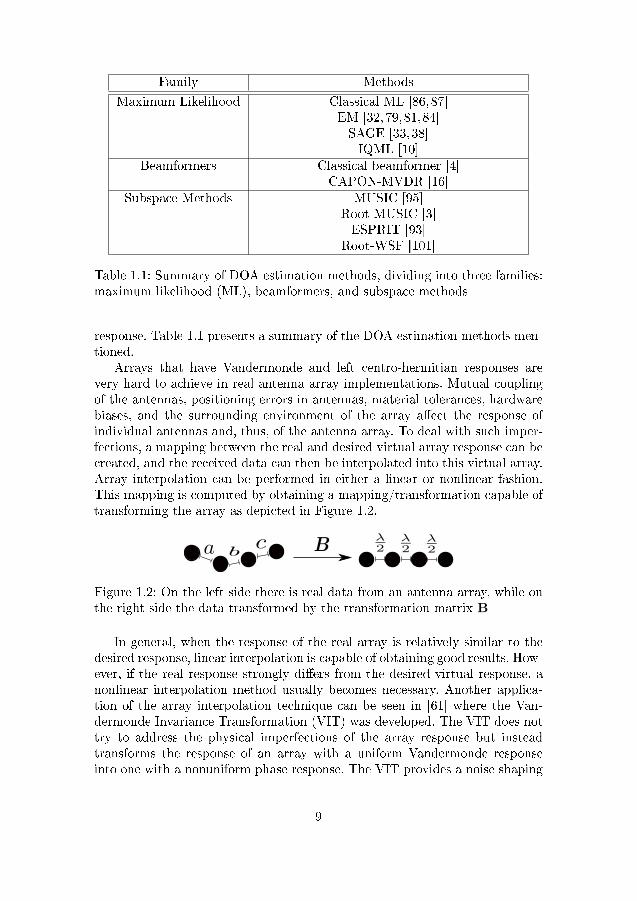
Table 1.1: Summary of DOA estimation methods, dividing into three families:maximum likelihood (ML), beamformers, and subspace methods

response. Table 1.1 presents a summary of the DOA estimation methods men-tioned.

Arrays that have Vandermonde and left centro-hermitian responses arevery hard to achieve in real antenna array implementations. Mutual couplingof the antennas, positioning errors in antennas, material tolerances, hardwarebiases, and the surrounding environment of the array a�ect the response ofindividual antennas and, thus, of the antenna array. To deal with such imper-fections, a mapping between the real and desired virtual array response can becreated, and the received data can then be interpolated into this virtual array.Array interpolation can be performed in either a linear or nonlinear fashion.This mapping is computed by obtaining a mapping/transformation capable oftransforming the array as depicted in Figure 1.2.

Figure 1.2: On the left side there is real data from an antenna array, while onthe right side the data transformed by the transformation matrix B

In general, when the response of the real array is relatively similar to thedesired response, linear interpolation is capable of obtaining good results. How-ever, if the real response strongly di�ers from the desired virtual response, anonlinear interpolation method usually becomes necessary. Another applica-tion of the array interpolation technique can be seen in [61] where the Van-dermonde Invariance Transformation (VIT) was developed. The VIT does nottry to address the physical imperfections of the array response but insteadtransforms the response of an array with a uniform Vandermonde responseinto one with a nonuniform phase response. The VIT provides a noise shaping

9

e�ect by lowering the noise power over a desired angular region and allowing amore precise DOA estimation at the cost an of increased computational load.

Bronez [11] �rst presented a solution for mapping real imperfect arrayresponses into precise and desired responses, and he has called such mappingarray interpolation. The presented schemes rely on dividing the �eld of view ofthe array response into smaller angular regions, called sectors. For each of thesesectors, a transformation matrix is calculated using the empirical knowledgeof the true array response. This is called sector-by-sector array interpolation.The larger the region transformed the larger the bias introduced becomes dueto transformation imprecision. Friedlander and Weiss [40] extended sector-by-sector array interpolation to include FBA, SPS, and DOA estimation algo-rithms such as Root-MUSIC [39]. Bühren et al. [13] presented a design metricfor the virtual array seeking to preserve the directional characteristics of thetrue array. Bühren et al. [12] and Weiss and Gavish [95] presented methods forarray interpolation that allow the application of ESPRIT for DOA estimation.All of these interpolation methods are performed on by sector-by-sector basis,dividing the entire �eld of view of the array and performing multiple DOAestimations, one for each sector.

When performing array interpolation for a sector there is no guarantee withrespect to what happens with signals received from outside the angular regionfor which the transformation matrix was derived (out-of-sector signals). If theout-of-sector signal is correlated with any possible in-sector signal, a largebias in the DOA estimation is introduced. Pesavento et al. [89] proposed amethod for �ltering out of sector signals using cone programming. A similarapproach was used by Lau et al. [63,64] where correlated out-of-sector signalswere addressed by �ltering out the out-of-sector signals.

More recently, array interpolation has been applied to more speci�c sce-narios. Liu et at. [68] extended the concept of linear array interpolation tocoprime arrays allowing for better identi�ability of received signals. Hosseiniand Sebt [52] applied the concept of linear array interpolation to sparse arraysby selecting virtual arrays as small as possible while retaining the aperture ofthe original sparse array.

This work proposes an adaptive single sector selection method aiming tocircumvent the problem of out-of-sector signals by interpolating all regions ofthe array where power is received using a single transformation. This workpresents an alternative for applying ESPRIT with FBA and SPS, relyingon a signal adaptive sector construction and discretization and extended themethod to the multidimensional case. The proposed method prevents out-of-sector problems by building a single sector using a signal adaptive approachwhile also bounding the transformation error. This, however, can lead to largesectors and, in the case of a small number of antennas, this will lead to largertransformation errors and DOA estimation biases. To deal with these limita-tions, the work at hand also presents a novel pre-processing step used for sectordiscretization based on PCA and derives a novel concept from the UT [74].

10

Furthermore, this work extends the concepts of linear interpolation and sectorselection to the muldimensional case, allowing the application of the proposedmethods is arrays and data models with an arbitrary number of dimensions.

This work proposes a novel nonlinear interpolation approach using MARS.The proposed approach is capable of interpolating arrays with a limited num-ber of antennas and very distorted responses while keeping the DOA estimationbias low, heavily outperforming array linear interpolation methods. This per-formance improvement comes at the cost of increased computational cost. Thiswork extends the MARS with advanced sector discretization methods that leadto a better performance and lower complexity. Furthermore, a more detailedmathematical description of the MARS method is presented. Expanding onthe topic of nonlinear interpolation, the work at hand additionally presentsan novel interpolation approach based on GRNNs. The proposed method iscapable of achieving a performance similar to that of MARS in certain SNRregimes at a lower computational cost compared to the MARS based method.

In summary, this work extends the concepts of array interpolation pre-sented in previous research to explore the concepts of statistical signi�cantsector discretization and nonlinear interpolation. Previous research focused onconcepts for sector-by-sector processing, whereas this work aims to use a singleuni�ed sector discretized in a statistically signi�cant manner. Moreover, thiswork develops novel nonlinear methods for array interpolation and presentsa method suitable for real-time implementations capable of providing betterperformance than linear interpolation methods previously derived in the liter-ature.

The results of the proposed discretization and interpolation methods are as-sessed via a set of studies considering measured responses obtained from a realphysical system. The results show that all the proposed methods signi�cantlyimprove DOA estimation considering a physical system and its inherent im-perfections. Furthermore, this work analyses the performance of the proposedinterpolation methods when measurements of the true array response are notavailable and only simulated responses for building the interpolation modelsare available.

1.3 Data Model

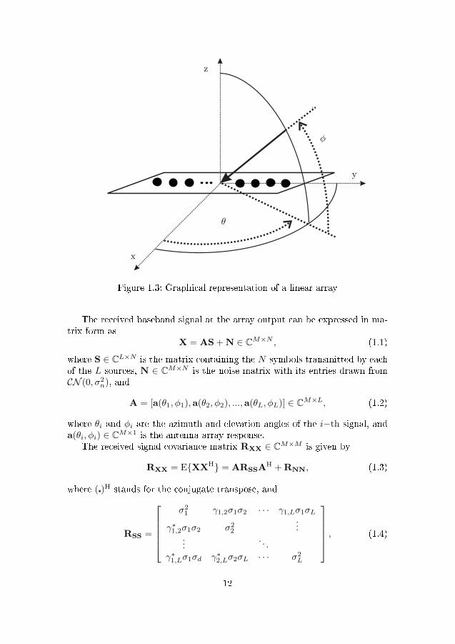
This model considers a set of L wavefronts impinging onto a linear antennaarray composed ofM antennas. Figure 1.3 shows a graphical representation ofthe linear array. Considering the antenna elements are placed along the y-axis,the array geometry can be used to estimate the azimuth angle θ. For arrayscomposed of isotropic antennas, the elevation angle φ would have no in�uenceon the antenna response, however, this work considers arrays with imperfectresponses that have varying amplitude and phase responses of the di�erentelements of the array with respect to the elevation angle of the received signals.

11

φ

θ

x

y

z

Figure 1.3: Graphical representation of a linear array

The received baseband signal at the array output can be expressed in ma-trix form as

X = AS + N ∈ CM×N , (1.1)

where S ∈ CL×N is the matrix containing the N symbols transmitted by eachof the L sources, N ∈ CM×N is the noise matrix with its entries drawn fromCN (0, σ2

n), and

A = [a(θ1, φ1),a(θ2, φ2), ...,a(θL, φL)] ∈ CM×L, (1.2)

where θi and φi are the azimuth and elevation angles of the i−th signal, anda(θi, φi) ∈ CM×1 is the antenna array response.

The received signal covariance matrix RXX ∈ CM×M is given by

RXX = E{XXH} = ARSSAH + RNN, (1.3)

where (�)H stands for the conjugate transpose, and

RSS =

σ2

1 γ1,2σ1σ2 · · · γ1,Lσ1σL

γ∗1,2σ1σ2 σ22

......

. . .

γ∗1,Lσ1σd γ∗2,Lσ2σL · · · σ2L

, (1.4)

12

where σ2i is the power of the i−th signal and γi,i′ ∈ C, |γi,i′ | ≤ 1 is the cross-

correlation coe�cient between signals i and i′with i 6= i′. RNN ∈ CM×M thespatial covariance matrix of the noise. In case the entries of the noise matrixare drawn from CN (0, σ2

n), RNN = IMσ2n , where IM denotes an M × M

identity matrix.An estimate of the received signal covariance matrix can be obtained by

RXX =XXH

N∈ CM×M . (1.5)

1.4 Preliminaries

In this section some important concepts used throughout the chapter are ex-plained. Subsections 1.4.1 and 1.4.2 present a brief overview of the FBA andSPS algorithms. The problem of model order selection is detailed in subsec-tion 1.4.3. The ESPRIT parameter estimation algorithm is shown in subsection1.4.4. Finally, subsection 1.4.5 explains the vandermonde invariance transfor-mation (VIT).

1.4.1 Forward Backward Averaging (FBA)

In the case where only two highly correlated or coherent sources are present theFBA [90] is capable of decorrelating the signals and allowing the applicationof subspace based methods. For an uniform linear array (ULA) or uniformrectangular array (URA) the steering vectors remain invariant, up to scaling,if their elements are reversed and complex conjugated. Let Q ∈ ZM×M by anexchange matrix with ones on its anti-diagonal and zeros elsewhere as de�nedin (A.1). Then, for a M element ULA it holds that

QA* = A. (1.6)

The forward backward averaged covariance matrix can be obtained as

RXXFBA=

1

2(RXX + QR∗XXQ). (1.7)

By looking into the structure of the covariance matrix shown in (1.3), (1.7)can be rewritten as

RXXFBA= A

1

2(RSS + R∗SS)AH +

1

2(RNN + QRNN

∗Q). (1.8)

The results is that the matrix RSS + R∗SS = 2<(RSS) is composed of purelyreal numbers, that is, if the correlation coe�cient between the signals is givenby a purely imaginary number then the FBA o�ers maximum decorrelation,if, however, the correlation coe�cient is given only by a real number, thenthe FBA o�ers no improvement regarding signal decorrelation. FBA can also

13

be used with the sole purpose of improving the variance of the estimates byvirtually doubling the number of available samples without resulting in noisecorrelation.

1.4.2 Spatial Smoothing (SPS)

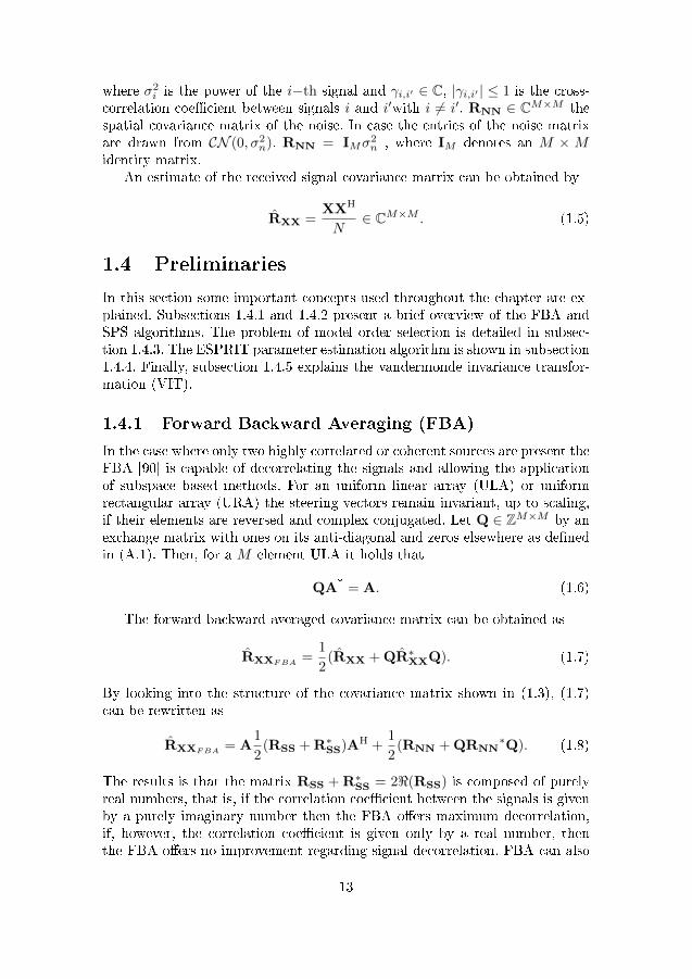
In scenarios where more than two highly correlated sources are present theFBA alone cannot restore the full rank of the signal covariance matrix byitself and thus another solution is necessary. SPS was �rst presented as aheuristic solution in [110] and extended to signal processing in [37]. The ideabehind Spatial Smoothing is to split a uniform array into multiple overlappingsubarrays as shown in Figure 1.4, the steering vectors of the subarrays are againassumed to be identical up to scaling. Therefore, the covariance matrices ofeach subarray can be averaged.

Figure 1.4: Example of SPS subarrays

Spatial Smoothing induces a random phase modulation that tends to decor-relate the signals that cause the rank de�ciency [59]. The SPS covariance ma-trix can be written as

RXXSPS=

1

V

V∑v=1

JvRXXJTv , (1.9)

where Jv is an appropriate selection matrix to select the signals of the respec-tive subarray.

The rank of the SPS covariance matrix can be shown to increase by 1with probability 1 [21] for each additional subarray used until it reaches themaximum rank of L. SPS however comes at the cost of reducing array aperture,since the subarrays are composed of less antennas than the original full array.

More details on FBA and SPS can be found in Appendix B.

1.4.3 Model Order Selection

Model order selection is selecting the optimal trade-o� between model resolu-tion and its statistical reliability. In the speci�c case of this work, model orderselection is mostly employed to select the eigenvectors of the signal covariancematrix that account for most of its power, each of these eigenvectors, in turn,

14

represents the statistics of a received signal. Therefore, in this work, modelorder selection is mostly used to estimate the number of signals received atthe antenna array. This is done by analyzing the pro�le of the eigenvalues ofthe signal covariance matrix and looking for a big gap that should separate theeigenvalues related to the signal from the ones related to the noise subspace.If the signals are highly correlated a single eigenvalue can be related to two ormore signals, leading to a biased estimation. For this reason, FBA and SPSmust be applied in such cases.

1 2 3 4 5 6 710

−4

10−3

10−2

10−1

100

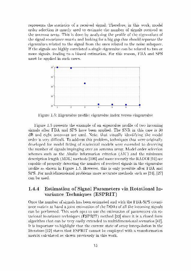
Figure 1.5: Eigenvalue pro�le: eigenvalue index versus eingenvalue

Figure 1.5 presents the example of an eigenvalue pro�le of two incomingsignals after FBA and SPS have been applied. The SNR in this case is 30dB and eight antennas are used. Note, that visually identifying the modelorder is very di�cult. To address this problem, techniques that were originallydeveloped for model �tting of statistical models were extended to detectingthe number of signals impinging over an antenna array. Model order selectionschemes such as the Akaike information criterion (AIC) and the minimumdescription length (MDL) methods [106] and more recently the RADOI [91] arecapable of properly detecting the number of received signals in the eigenvaluepro�le as shown in Figure 1.5. However, this is only possible after FBA andSPS. For multidimensional problems more accurate methods such as [24], [27]can be used.

1.4.4 Estimation of Signal Parameters via Rotational In-variance Techniques (ESPRIT)

Once the number of signals has been estimated and with the FBA-SPS covari-ance matrix at hand a joint estimation of the DOAs of all the incoming signalscan be performed. This work opts to use the estimation of parameters via ro-tational invariance techniques (ESPRIT) method [93] since it is a closed formalgorithm that can be very easily extended to multidimensional scenarios [47].It is important to highlight that the current state of array interpolation in theliterature [12] states that ESPRIT cannot be employed with a transformationmatrix calculated as shown previously in this work.

15

The ESPRIT parameter estimation technique is based on subspace de-composition. Matrix subspace decomposition is usually done by applying theSingular Value Decomposition (SVD). The SVD of the matrix X∈ CM×N isgiven by

X = UΣVH, (1.10)

where U ∈ CM×M and VN×N are unitary matrices called the left-singularvectors and right-singular vectors of X and Σ ∈ CM×N is pseudo diagonal

matrix containing the singular values of X. The signal subspace ES ∈ CM×Lof X can be constructed by selecting only the singular vectors related to the Llargest singular values, the remaining singular vectors form the noise subspace

EN ∈ CM×M−L of X.Equivalently eigenvalue decomposition can be applied on the auto correla-

tion matrix RXX of X spanning the same subspace

RXX = EΛE−1, (1.11)

where E ∈ CM×M and Λ ∈ CM×M contains the eigenvectors and eigenvaluesof RXX. The eigenvectors related to the L largest eigenvalues span the samesignal subspace ES of the single value decomposition. The same holds for thenoise subspace of the EVD and left singular vectors of the SVD, EN .

This classic eigendecomposition is suitable when the noise received at theantenna array is spatially white, since, in the case at hand, a transformationis applied to the data, even if the received noise was originally white it turnsin colored noise. To deal with colored noise the generalized eigenvalue decom-position (GEVD) can be used to take the noise correlation into account, theGEVD of the matrix pair RXX, RNN is given by

RXXΓ = RNNΓΛ, (1.12)

where E ∈ CM×M is a matrix containing the generalized eigenvectors andΛ ∈ RM×M is a matrix containing the generalized eigenvalues in its diagonal.Notice that this decomposition is the same as the EVD (1.11) for RNN = I.

The subspace ΓS ∈ CM×L is formed selecting the generalized eigenvectorsrelated to the L largest generalized eigenvalues. This subspace, however, doesnot span the same column subspace as the original steering matrix, and needsto be reprojected onto the original manifold subspace or dewhitened. This canbe done by

Γs = RNNΓs. (1.13)

With this subspace estimate at hand the Total Least Squares (TLS) ESPRIT[93] is applied. Two subsets of the signal subspace that are related trough theshift invariance property need to be selected.

Let Γ1 and Γ2 represent the subspace subsets selected as previously men-tioned. A matrix Γ1,2 is constructed as

Γ1,2 =

[ΓH

1

ΓH2

][Γ1Γ2] . (1.14)

16

Performing an eigendecomposition of Γ1,2 and ordering its eigenvalues in thedecreasing order and its eigenvectors accordingly the eigenvector matrix V canbe divided into blocks as

V =

[V1,1 V1,2

V2,1 V2,2

]. (1.15)

Finally, the parameters can be obtained by �nding the eigenvalues of

Φ = eig

(−V1,2

V2,2

). (1.16)

The parameters in Φ can represent a phase delay respective to a DOA if DOAsare being estimated, or can represent the ratio of the strength at which a signalappears in the di�erent polarizations.

For multidimensional arrays another option is to employ methods basedon the parallel factor analysis (PARAFAC) decomposition such as [29], [28]instead of the ESPRIT.

1.4.5 Vandermonde Invariance Transformation (VIT)

Finally, once the �rst set of estimates has been obtained the VIT can be ap-plied, this transformation aims to shape the noise away from the regions wherethe signal is arriving in order to obtain improved estimates [61] . The VIT isan array interpolation approach that transforms a vandermonde system witha response linear with respect to the angle of arrival into an also vandermondesystem with a highly nonlinear response with respect to the angle of arrival.The VIT promotes a nonlinear transformation with respect to the selectedspatial frequency µ(θ). Let u = [1, ejµ(θ), . . . , ejµ(θ)(M−1)], the VIT performsthe following transformation

u(V IT ) = T(θ)u = (ejµ(θ) − r

1− r )

1

ejν(θ)

...ejν(θ)(M−1)

, (1.17)

r and ν are design parameters that can be chosen considering a compromisebetween the level of noise suppression desired around µ and the linearity ofthe output.

The VIT can be used to apply a phase attenuation to the dataset, whichin turn shapes the noise, reducing the power of the noise in the region nearµ(θ) and increasing it over its vicinity. Thus, the VIT needs to be appliedangle wise, i.e, a set of initial estimates of the angles θ is used to calculatea VIT centered over the given angles, and a second estimate is performed.This second estimation yields and o�set θoffset with respect to the originalθ, giving the �nal estimation θVIT = θ + θoffset. Due to the mentioned noise

17

shaping, this �nal estimation o�ers increased precision, but comes at the costof transforming the dataset and applying the chosen DOA estimation methodL times.

The VIT can be interpreted as a zoom, similar to an optical zoom, with the�rst estimates a zoom can be used on the regions of the manifold where signalhas been estimated to arrive. The region can be inspected with the zoom e�ectto detect any imprecisions from the �rst estimate. The increased performancecomes at the cost of L extra DOA estimations.

1.5 Array Interpolation

Arrays can be interpolated by means of a one-to-one mapping given by

f : AS → AS , (1.18)

where S is a sector. It is worth noting that even if an array has the requiredgeometry for the usage of a certain array processing technique, its responsemay not adhere to an underlying assumed mathematical model. Therefore, insuch cases, geometrically well behaved arrays may need to be interpolated toallow the application of the desired technique.

De�nition 1.1. A sector S is a �nite and countable set of 2-tuples (pairs) ofangles (θ, φ) containing all the combinations of azimuth and elevation anglesrepresenting a region of the �eld of view of the array. The sector S de�nes thecolumn space of AS and AS .

AS ∈ CM×|S| is the array response matrix formed out of the array re-sponse vectors a(θ, φ) ∈ CM×1 of the angles given by the elements of S. AScontains the true array response of the physical system, which may not pos-sess important properties such as being left centro-hermitian or Vandermonde.AS ∈ CM ′×|S| is the interpolated version of AS with columns a(θ, φ) ∈ CM ′×1

being the array response of the so-called virtual or desired array, having allthe properties necessary for posterior processing. |S| is the cardinality of theset S, i.e. the number of elements in the set.

De�nition 1.2. The mapping f is said to be array size preserving ifM = M ′.

De�nition 1.3. The mapping f is said to be geometry preserving if it is sizepreserving and if the underlying array geometry for the true and virtual arrayis equivalent.

This work limits itself to mappings of linear planar arrays that are size andgeometry preserving, as given in De�nitions 1.2 and 1.3, respectively.

Linear array interpolation is usually done using a least squares approach.The problem is set up as �nding a transformation matrix B that is given by

BAS = AS . (1.19)

18

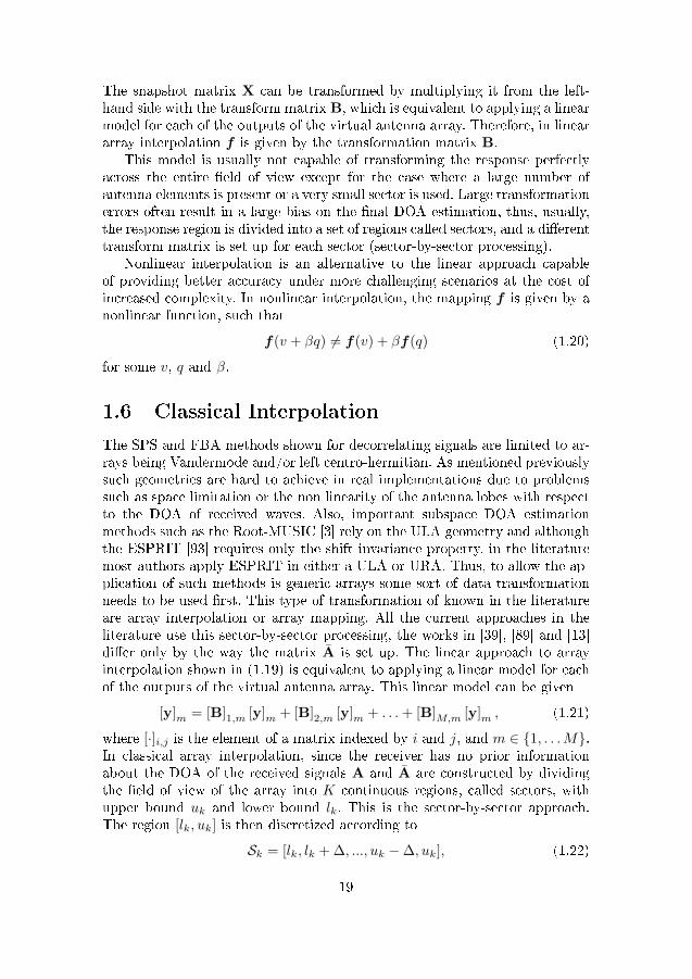
The snapshot matrix X can be transformed by multiplying it from the left-hand side with the transform matrix B, which is equivalent to applying a linearmodel for each of the outputs of the virtual antenna array. Therefore, in lineararray interpolation f is given by the transformation matrix B.

This model is usually not capable of transforming the response perfectlyacross the entire �eld of view except for the case where a large number ofantenna elements is present or a very small sector is used. Large transformationerrors often result in a large bias on the �nal DOA estimation, thus, usually,the response region is divided into a set of regions called sectors, and a di�erenttransform matrix is set up for each sector (sector-by-sector processing).

Nonlinear interpolation is an alternative to the linear approach capableof providing better accuracy under more challenging scenarios at the cost ofincreased complexity. In nonlinear interpolation, the mapping f is given by anonlinear function, such that

f(v + βq) 6= f(v) + βf(q) (1.20)

for some v, q and β.

1.6 Classical Interpolation

The SPS and FBA methods shown for decorrelating signals are limited to ar-rays being Vandermode and/or left centro-hermitian. As mentioned previouslysuch geometries are hard to achieve in real implementations due to problemssuch as space limitation or the non linearity of the antenna lobes with respectto the DOA of received waves. Also, important subspace DOA estimationmethods such as the Root-MUSIC [3] rely on the ULA geometry and althoughthe ESPRIT [93] requires only the shift invariance property, in the literaturemost authors apply ESPRIT in either a ULA or URA. Thus, to allow the ap-plication of such methods is generic arrays some sort of data transformationneeds to be used �rst. This type of transformation of known in the literatureare array interpolation or array mapping. All the current approaches in theliterature use this sector-by-sector processing, the works in [39], [89] and [13]di�er only by the way the matrix A is set up. The linear approach to arrayinterpolation shown in (1.19) is equivalent to applying a linear model for eachof the outputs of the virtual antenna array. This linear model can be given

[y]m = [B]1,m [y]m + [B]2,m [y]m + . . .+ [B]M,m [y]m , (1.21)

where [·]i,j is the element of a matrix indexed by i and j, and m ∈ {1, . . .M}.In classical array interpolation, since the receiver has no prior informationabout the DOA of the received signals A and A are constructed by dividingthe �eld of view of the array into K continuous regions, called sectors, withupper bound uk and lower bound lk. This is the sector-by-sector approach.The region [lk, uk] is then discretized according to

Sk = [lk, lk + ∆, ..., uk −∆, uk], (1.22)

19

where ∆ is the angular resolution of the transformation. These angles areused to generate the respective set of steering vectors and construct A and Aaccording to

ASk = [a(lk),a(lk + ∆), ...,a(uk −∆),a(uk)] ∈ CM×uk−lk

∆ ,

ASk = [a(lk), a(lk + ∆), ..., a(uk −∆), a(uk)] ∈ CM×uk−lk

∆ ,

where M is the number of antennas, including their di�erent polarizations,present at the array. The transformation is usually not perfect since the trans-formation matrix B does not have enough degrees of freedom to transform theentire discrete sector. B is obtained as the best �t between the transformedresponse BASk and the desired response ASk , this is done by applying a leastsquares �t to the overdetermined systems yielding

B = ASkA†Sk ∈ CM×M , (1.23)

where (·)† is the pseudo inverse of the matrix. To access the precision of thetransformation the Frobenius norm of the errors matrix BASk − ASk is com-pared with the Frobenius norm of the desired response steering matrix ASk .The error of the transform is de�ned as

ε(Sk) =

∥∥ASk −BASk∥∥

F∥∥ASk∥∥F

∈ R+. (1.24)

Large transformation errors will results in a large bias in the �nal DOA esti-mates. The transformation error can, however, be kept as low as desired bymaking the sectors Sk smaller. It is worth noting that for the sector-by-sectorapproach the transformation matrices can be calculated o�-line, since they donot rely on the received data, and just reused when necessary.

With B at hand the data can be transformed by

X = BX. (1.25)

The transformed covariance is then equivalent to

RXX =BX(BX)H

N=

BXXHBH

N= BRXXBH. (1.26)

From (1.26) it is possible to note that the transformation matrix can insteadbe applied directly to the covariance matrix. Plugging (1.4) into (1.26) resultsin

RXX = BARSSAHBH + BRNNBH (1.27)

= ARSSAH + BRNNBH.

Thus, although the transformation transforms A into A as desired it changesthe characteristics of RNN. If the noise was previously white it becomes colored

20

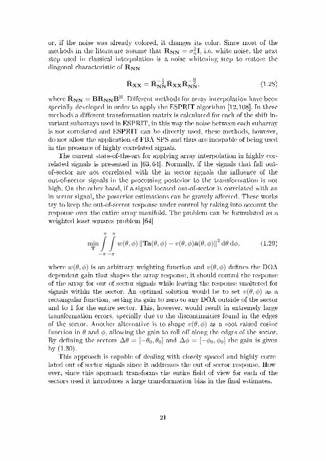
or, if the noise was already colored, it changes its color. Since most of themethods in the literature assume that RNN = σ2

nI, i.e, white noise, the nextstep used in classical interpolation is a noise whitening step to restore thediagonal characteristic of RNN

RXX = R− 1

2

NNRXXR−H

2

NN, (1.28)

where RNN = BRNNBH. Di�erent methods for array interpolation have beenspecially developed in order to apply the ESPRIT algorithm [12,108]. In thesemethods a di�erent transformation matrix is calculated for each of the shift in-variant subarrays used in ESPRIT, in this way the noise between each subarrayis not correlated and ESPRIT can be directly used, these methods, however,do not allow the application of FBA-SPS and thus are incapable of being usedin the presence of highly correlated signals.

The current state-of-the-art for applying array interpolation in highly cor-related signals is presented in [63, 64]. Normally, if the signals that fall out-of-sector are not correlated with the in sector signals the in�uence of theout-of-sector signals in the processing posterior to the transformation is nothigh. On the other hand, if a signal located out-of-sector is correlated with anin sector signal, the posterior estimations can be gravely a�ected. These workstry to keep the out-of-sector response under control by taking into account theresponse over the entire array manifold. The problem can be formulated as aweighted least squares problem [64]

minT

π∫−π

π∫−π

w(θ, φ) ‖Ta(θ, φ)− v(θ, φ)a(θ, φ)‖2 dθ dφ, (1.29)

where w(θ, φ) is an arbitrary weighting function and v(θ, φ) de�nes the DOAdependent gain that shapes the array response, it should control the responseof the array for out-of-sector signals while leaving the response unaltered forsignals within the sector. An optimal solution would be to set v(θ, φ) as arectangular function, setting its gain to zero to any DOA outside of the sectorand to 1 for the entire sector. This, however, would result in extremely largetransformation errors, specially due to the discontinuities found in the edgesof the sector. Another alternative is to shape v(θ, φ) as a root raised cosinefunction in θ and φ, allowing the gain to roll o� along the edges of the sector.By de�ning the sectors ∆θ = [−θ0, θ0] and ∆φ = [−φ0, φ0] the gain is givenby (1.30).

This approach is capable of dealing with closely spaced and highly corre-lated out-of-sector signals since it addresses the out-of-sector response. How-ever, since this approach transforms the entire �eld of view for each of thesectors used it introduces a large transformation bias in the �nal estimates.

21

v(θ,φ

)=

1,

|θ|≤

θ 0an

d|φ|≤

φ0

1 2+

1 4co

s(π

(|θ|−θ0)

2θ0−π

)+

1 4co

s(π

(|φ|−φ

0)

2φ

0−π

),θ 0<|θ|≤

(π−θ 0

)orφ

0<|φ|≤

(π−φ

0)

0,(π−θ 0

)<|θ|≤π

or

(π−φ

0)<|φ|≤

π

(1.30)

22

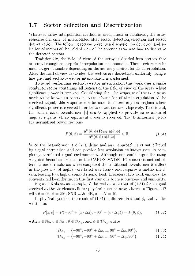
1.7 Sector Selection and Discretization

Whatever array interpolation method is used, linear or nonlinear, the arrayresponse can only be interpolated after sector detection/selection and sectordiscretization. The following section presents a discussion on detection and se-lection of sectors of the �eld of view of the antenna array and how to discretizethe detected sectors.

Traditionally, the �eld of view of the array is divided into sectors thatare small enough to keep the interpolation bias bounded. These sectors can bemade larger or smaller depending on the accuracy desired for the interpolation.After the �eld of view is divided the sectors are discretized uniformly using a�ne grid and sector-by-sector interpolation is performed.

To avoid performing sector-by-sector interpolation this work uses a singlecombined sector containing all regions of the �eld of view of the array wheresigni�cant power is received. Considering that the response of the true arrayneeds to be known to construct a transformation of the interpolation of thereceived signal, this response can be used to detect angular regions wheresigni�cant power is received in order to detect sectors adaptively. To this end,the conventional beamformer [4] can be applied to provide an estimate ofangular regions where signi�cant power is received. The beamformer yieldsthe normalized power response

P (θ, φ) =aH(θ, φ) RXX a(θ, φ)

aH(θ, φ) a(θ, φ)∈ R. (1.31)

Since the beamformer is only a delay and sum approach it is not a�ectedby signal correlation and can provide low resolution estimates even in com-pletely correlated signal environments. Although one could argue for usingweighted beamformers such as the CAPON-MVDR [16] since this method of-fers increased resolution when compared the traditional beamformer it su�ersin the presence of highly correlated wavefronts and requires a matrix inver-sion, leading to a higher computational load. Therefore, this work employs theconventional beamformer in this �rst step due to its robustness and simplicity.

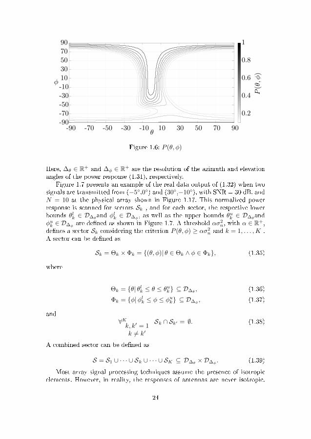
Figure 1.6 shows an example of the real data output of (1.31) for a signalreceived at the six element linear physical antenna array shown in Figure 1.17with θ = 0◦, φ = 20◦, SNR = 30 dB, and N = 10.

In physical systems, the result of (1.31) is discrete in θ and φ, and can bewritten as

P [z, v] = P (−90◦ + (z ·∆θ),−90◦ + (v ·∆φ)) = P (θ, φ), (1.32)

with z ∈ N0, v ∈ N0 , θ ∈ D∆θ, and φ ∈ D∆φ

where

D∆θ= {−90◦,−90◦ + ∆θ, ..., 90◦ −∆θ, 90◦}, (1.33)

D∆φ= {−90◦,−90◦ + ∆φ, ..., 90◦ −∆φ, 90◦}. (1.34)

23

-90 -70 -50 -30 -10 10 30 50 70 90-90

-70

-50

-30

-10

10

30

50

70

90

0.2

0.4

0.6

0.8

1

φ

P(θ,φ

)

θ

Figure 1.6: P (θ, φ)

Here, ∆θ ∈ R+ and ∆φ ∈ R+ are the resolution of the azimuth and elevationangles of the power response (1.31), respectively.

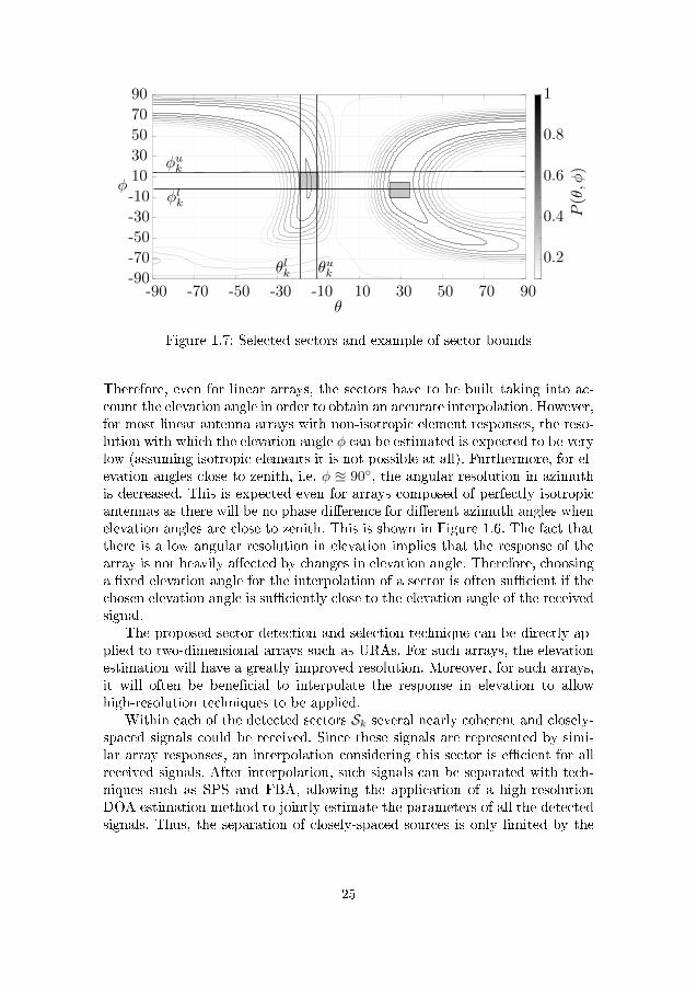
Figure 1.7 presents an example of the real data output of (1.32) when twosignals are transmitted from (−5◦,0◦) and (30◦,−10◦), with SNR = 30 dB, andN = 10 at the physical array shown in Figure 1.17. This normalized powerresponse is scanned for sectors Sk , and for each sector, the respective lowerbounds θlk ∈ D∆θ

and φlk ∈ D∆φ, as well as the upper bounds θuk ∈ D∆θ

andφuk ∈ D∆φ

are de�ned as shown in Figure 1.7. A threshold ασ2n, with α ∈ R+,

de�nes a sector Sk considering the criterion P (θ, φ) ≥ ασ2n and k = 1, . . . ,K .

A sector can be de�ned as

Sk = Θk × Φk = {(θ, φ)| θ ∈ Θk ∧ φ ∈ Φk}, (1.35)

where

Θk = {θ| θlk ≤ θ ≤ θuk} ⊆ D∆θ, (1.36)

Φk = {φ|φlk ≤ φ ≤ φuk} ⊆ D∆φ, (1.37)

and∀Kk, k′ = 1k 6= k′

Sk ∩ Sk′ = ∅. (1.38)

A combined sector can be de�ned as

S = S1 ∪ · · · ∪ Sk ∪ · · · ∪ SK ⊆ D∆θ×D∆φ

. (1.39)

Most array signal processing techniques assume the presence of isotropicelements. However, in reality, the responses of antennas are never isotropic.

24

-90 -70 -50 -30 -10 10 30 50 70 90-90

-70

-50

-30

-10

10

30

50

70

90

0.2

0.4

0.6

0.8

1

P(θ,φ

)

θ

φ

θlk θuk

φlk

φuk

Figure 1.7: Selected sectors and example of sector bounds

Therefore, even for linear arrays, the sectors have to be built taking into ac-count the elevation angle in order to obtain an accurate interpolation. However,for most linear antenna arrays with non-isotropic element responses, the reso-lution with which the elevation angle φ can be estimated is expected to be verylow (assuming isotropic elements it is not possible at all). Furthermore, for el-evation angles close to zenith, i.e. φ u 90◦, the angular resolution in azimuthis decreased. This is expected even for arrays composed of perfectly isotropicantennas as there will be no phase di�erence for di�erent azimuth angles whenelevation angles are close to zenith. This is shown in Figure 1.6. The fact thatthere is a low angular resolution in elevation implies that the response of thearray is not heavily a�ected by changes in elevation angle. Therefore, choosinga �xed elevation angle for the interpolation of a sector is often su�cient if thechosen elevation angle is su�ciently close to the elevation angle of the receivedsignal.

The proposed sector detection and selection technique can be directly ap-plied to two-dimensional arrays such as URAs. For such arrays, the elevationestimation will have a greatly improved resolution. Moreover, for such arrays,it will often be bene�cial to interpolate the response in elevation to allowhigh-resolution techniques to be applied.

Within each of the detected sectors Sk several nearly coherent and closely-spaced signals could be received. Since these signals are represented by simi-lar array responses, an interpolation considering this sector is e�cient for allreceived signals. After interpolation, such signals can be separated with tech-niques such as SPS and FBA, allowing the application of a high-resolutionDOA estimation method to jointly estimate the parameters of all the detectedsignals. Thus, the separation of closely-spaced sources is only limited by the

25

high-resolution DOA estimation method and by the number of elements of theantenna array, but not by the array interpolation itself.

To address cases where the noise �oor is high a large α can be used. How-ever, this means that only large sectors are detected, at the cost of discardingsmaller sectors that are related to a signal component. On the other hand,smaller α means that smaller sectors are detected but at the cost of allowingnoise to be mistakenly detected as a sector. Selecting noise regions as sectorswill results in a smaller estimation bias than leaving regions with signal powerout of the transform. Therefore, for cases where the noise �oor is high com-pared to the signal strength, an α that sets the cuto� to be close to the noise�oor is recommended.

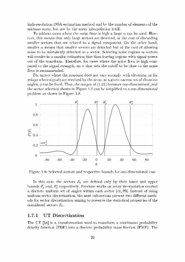
For arrays where the response does not vary strongly with elevation, or forsetups where signals are received by the array at a given narrow set of elevationangles, φ can be �xed. Thus, the output of (1.31) becomes one-dimensional, andthe sector selection shown in Figure 1.7 can be simpli�ed to a one-dimensionalproblem as shown in Figure 1.8.

-80 -60 -40 -20 0 20 40 60 800

0.2

0.4

0.6

0.8

1

ασ2n

θl1 θu1 θl2 θu2

θ

P(θ)

Figure 1.8: Selected sectors and respective bounds for one-dimensional case

In this case, the sectors Sk are de�ned only by their lower and upperbounds θlk and, θ

uk respectively. Previous works on array interpolation created

a discrete uniform set of angles within each sector [11, 89]. Instead of usinguniform sector discretization, the next subsections present two di�erent meth-ods for sector discretization aiming to preserve the statistical properties of theconsidered sectors Sk.

1.7.1 UT Discretization

The UT [54] is a transformation used to transform a continuous probabilitydensity function (PDF) into a discrete probability mass �nction (PMF). The

26

UT can be applied in array interpolation to discretize the detected sectorsin such a way that the statistical properties, the moments, of the detectedsectors are preserved in its discrete form. Thus, no statistical information islost, since a PDF can be fully represented by its moments as stated in thefollowing theorem.

Theorem 1. A probability density function can be entirely described by itsmoments.

Proof. A proof can be found in Appendix C.

The UT discretization can be applied by solving the nonlinear set of equa-tions

k−1∑j=1

wjSkj = w1S

k1 + ...+ wk−1S

kk−1 = E{rk}. (1.40)

where Sj are known as sigma points, wj are its respective weights, and r is thevalue assumed by a continuous random variable r. From (1.40) it is clear that inorder to preserve the characteristics of r up to the k-th moment, it is necessaryto calculate k − 1 sigma points and its weights by solving a nonlinear systemof equations. Thus, there is a trade-o� between simplicity in the calculationand the accuracy of the representation of higher order moments.

The UT can be applied to an approximation of the concentrated loss func-tion lc(X;θ,φ) and thus the log-likelihood l(X;θ,φ) of the DOA estimationproblem, which is derived in the following theorem. The concentrated lossfunction lc(X;θ,φ) and the log-likelihood l(X;θ,φ) of the DOA estimationproblem at hand are de�ned in (D.1) and (D.4), and

θ = [θ1, . . . , θd]T, (1.41)

φ = [φ1, . . . , φd]T. (1.42)

Theorem 2. The concentrated loss function lc(X;θ,φ) for a DOA estimationproblem can be approximated for each detected sector Sk by the normalizedpower response of the conventional beamformer (1.31).

Proof. A proof can be found in Appendix D.

Following the approximation derived in Theorem 2 the concentrated lossfunction and thus the log-likelihood with respect to each sector Sk can beconsidered as a separate PDF each when applying the UT. In order to pre-serve the �rst and the second moment of the approximated log-likelihood, thenumber of points are chosen to transform each detected sector Sk must belarger or equal than 3. Under this constraint and under the assumption thatthe input noise follows CN (0, σ2

n), the respective PDF characteristics for eachsector Sk are mainly preserved. Figure 1.9 presents how the concentrated loss

27

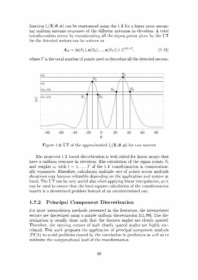
function lc(X;θ,φ) can be represented using the UT for a linear array assum-ing uniform antenna responses of the di�erent antennas in elevation. A totaltransformation sector by concatenating all the sigma points given by the UTfor the detected sectors can be written as

AS = [a(S1),a(S2), ...,a(ST )] ∈ CM×T , (1.43)

where T is the total number of points used to discretize all the detected sectors.

-80 -60 -40 -20 0 20 40 60 80

ω1, ω3

ω4, ω6

ω2

ω5

|w| S1

S2

S3

S4

S5

S6

θ

Figure 1.9: UT of the approximated lc(X;θ,φ) for two sources

The proposed UT-based discretization is well suited for linear arrays thathave a uniform response in elevation. The calculation of the sigma points Stand weights ωt with t = 1, . . . , T of the UT transformation is computation-ally expensive. Therefore, calculating multiple sets of points across multipleelevations may become infeasible depending on the application and system athand. The UT can be very useful also when applying linear interpolation, as itcan be used to ensure that the least squares calculation of the transformationmatrix is a determined problem instead of an overdetermined one.

1.7.2 Principal Component Discretization

For most interpolation methods presented in the literature, the interpolatedsectors are discretized using a simple uniform discretization [11, 89]. The dis-cretization is usually done such that the discrete angles are closely spaced.Therefore, the steering vectors of such closely spaced angles are highly cor-related. This work proposes the application of principal component analysis(PCA) to avoid problems caused by the correlation in predictors as well as tominimize the computational load of the transformation.

28

Ideally, AS would be set up such that ASAHS = IM . However, as stated

previously, this is often not the case with ASAHS = RASAS 6= IM . PCA aims

to �nd a matrix P such that

PAS = BS , (1.44)

where BSBHS = IM . P can be obtained by performing the eigendecomposition

of RASAS

RASAS = EΣEH, (1.45)

and setting P = E. The proposed PCA pre-processing can be used to createa better set of predictor variables for the interpolation and to reduce thedimensionality of the problem by excluding any eigenvectors associated tovery small eigenvalues.

1.8 Linear Adaptive Array Interpolation

In the case of linear interpolation, the transformation bias is closely tied tothe total size of the transformed sector. While the UT and PCA discretizationcan minimize this problem, they cannot fully mitigate it. Therefore, this thesispresents an iterative approach that seeks to �nd out the maximum region ofthe �eld of view that can be transformed while keeping the transformationerror bounded by a value. It also distributes the calculated region with respectto the power of each sector detected in the second step.

The �rst part of the next two steps is to calculate a weighting factor basedon the power of each detected sector. This weighting factor will be used to op-timally distribute the transformable region with respect to the received power,focusing the transformation on regions with more power and aiming to leavethe least signi�cant power outside of the total transformed region. Consider-ing a one dimensional beamformer output, a weighting factor for each sectoris calculated as

ξw =

∑θuwz=θlw

P [z]∑Wc=1

∑θucz=θlc

P [z]∈ R. (1.46)

As mentioned in Section 1.6, classical array interpolation methods in theliterature divide the array response into various sectors (sector-by-sector pro-cessing) in order to keep the error (1.24) small. However, in this thesis a singletransform matrix is used based on a combination of the sectors detected in(1.31). In order to bound the error ε(S) a signal adaptive method for calcu-lating the maximum transform size is used based on the weights calculated in(1.46). For a sector centered at µk, where

µk =

⌈θuk − θlk

2

⌋D∆

,

29

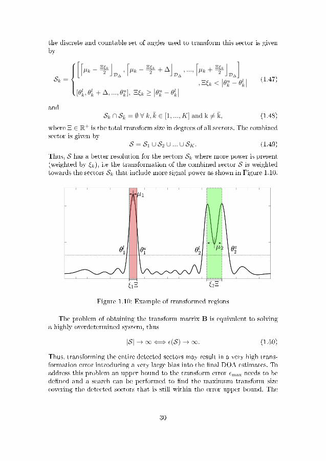
the discrete and countable set of angles used to transform this sector is givenby

Sk =

[⌈µk − Ξξk

2

⌋D∆

,⌈µk − Ξξk

2 + ∆⌋D∆

, ...,⌈µk + Ξξk

2

⌋D∆

],Ξξk <

∣∣θuk − θlk∣∣[θlk, θ

lk + ∆, ..., θuk ], Ξξk ≥

∣∣θuk − θlk∣∣(1.47)

andSk ∩ Sk = ∅ ∀ k, k ∈ [1, ...,K] and k 6= k, (1.48)

where Ξ ∈ R+ is the total transform size in degrees of all sectors. The combinedsector is given by

S = S1 ∪ S2 ∪ ... ∪ SK . (1.49)

Thus, S has a better resolution for the sectors Sk where more power is present(weighted by ξk), i.e the transformation of the combined sector S is weightedtowards the sectors Sk that include more signal power as shown in Figure 1.10.

Brasil Hexa Champion!!!

Figure 1.10: Example of transformed regions

The problem of obtaining the transform matrix B is equivalent to solvinga highly overdetermined system, thus

|S| → ∞ ⇐⇒ ε(S)→∞. (1.50)

Thus, transforming the entire detected sectors may result in a very high trans-formation error introducing a very large bias into the �nal DOA estimates. Toaddress this problem an upper bound to the transform error εmax needs to bede�ned and a search can be performed to �nd the maximum transform sizecovering the detected sectors that is still within the error upper bound. The

30

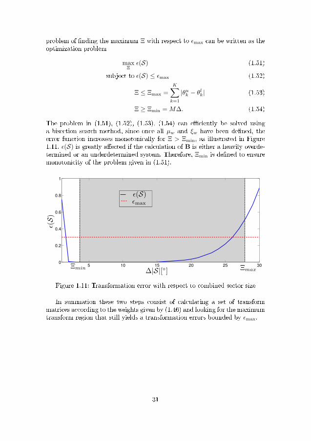
problem of �nding the maximum Ξ with respect to εmax can be written as theoptimization problem

maxΞ

ε(S) (1.51)

subject to ε(S) ≤ εmax (1.52)

Ξ ≤ Ξmax =

K∑k=1

|θuk − θlk| (1.53)

Ξ ≥ Ξmin = M∆. (1.54)

The problem in (1.51), (1.52), (1.53), (1.54) can e�ciently be solved usinga bisection search method, since once all µw and ξw have been de�ned, theerror function increases monotonically for Ξ > Ξmin, as illustrated in Figure1.11. ε(S) is greatly a�ected if the calculation of B is either a heavily overde-termined or an underdetermined system. Therefore, Ξmin is de�ned to ensuremonotonicity of the problem given in (1.51).

5 10 15 20 25 300

0.2

0.4

0.6

0.8

1

Figure 1.11: Transformation error with respect to combined sector size

In summation these two steps consist of calculating a set of transformmatrices according to the weights given by (1.46) and looking for the maximumtransform region that still yields a transformation errors bounded by εmax.

31

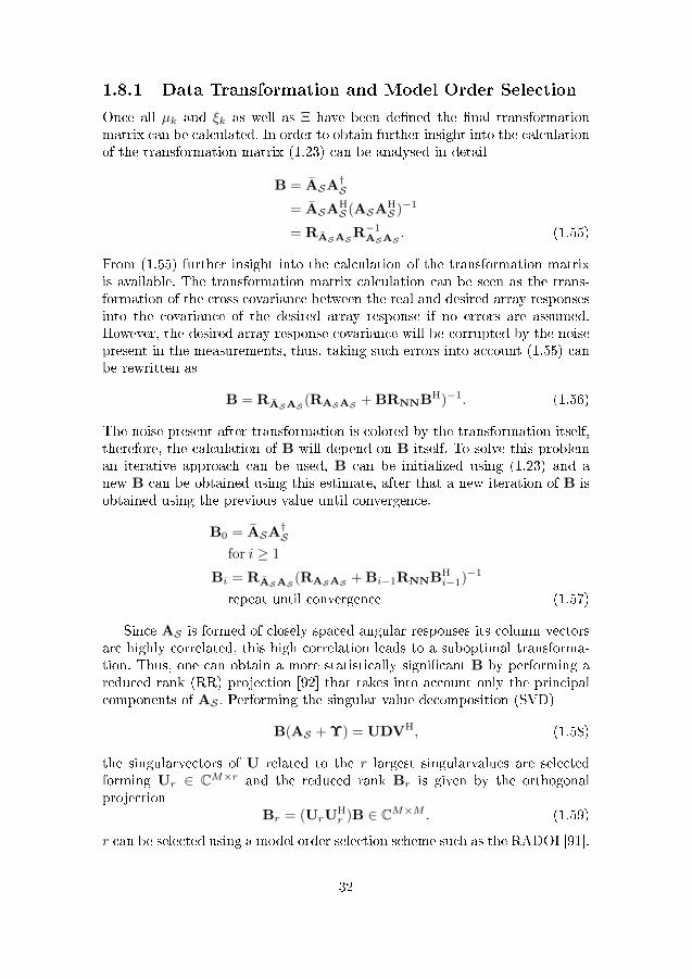
1.8.1 Data Transformation and Model Order Selection

Once all µk and ξk as well as Ξ have been de�ned the �nal transformationmatrix can be calculated. In order to obtain further insight into the calculationof the transformation matrix (1.23) can be analysed in detail

B = ASA†S

= ASAHS (ASA

HS )−1

= RASASR−1ASAS

. (1.55)

From (1.55) further insight into the calculation of the transformation matrixis available. The transformation matrix calculation can be seen as the trans-formation of the cross covariance between the real and desired array responsesinto the covariance of the desired array response if no errors are assumed.However, the desired array response covariance will be corrupted by the noisepresent in the measurements, thus, taking such errors into account (1.55) canbe rewritten as

B = RASAS (RASAS + BRNNBH)−1. (1.56)

The noise present after transformation is colored by the transformation itself,therefore, the calculation of B will depend on B itself. To solve this probleman iterative approach can be used, B can be initialized using (1.23) and anew B can be obtained using this estimate, after that a new iteration of B isobtained using the previous value until convergence.

B0 = ASA†S

for i ≥ 1

Bi = RASAS (RASAS + Bi−1RNNBHi−1)−1

repeat until convergence (1.57)

Since AS is formed of closely spaced angular responses its column vectorsare highly correlated, this high correlation leads to a suboptimal transforma-tion. Thus, one can obtain a more statistically signi�cant B by performing areduced rank (RR) projection [92] that takes into account only the principalcomponents of AS . Performing the singular value decomposition (SVD)

B(AS + Υ) = UDVH, (1.58)

the singularvectors of U related to the r largest singularvalues are selectedforming Ur ∈ CM×r and the reduced rank Br is given by the orthogonalprojection

Br = (UrUHr )B ∈ CM×M . (1.59)

r can be selected using a model order selection scheme such as the RADOI [91].

32

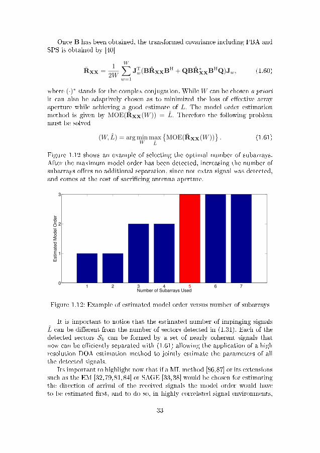
Once B has been obtained, the transformed covariance including FBA andSPS is obtained by [40]

RXX =1

2W

W∑w=1

JTw(BRXXBH + QBR∗XXBHQ)Jw, (1.60)

where (·)∗ stands for the complex conjugation. WhileW can be chosen a prioriit can also be adaptively chosen as to minimized the loss of e�ective arrayaperture while achieving a good estimate of L. The model order estimationmethod is given by MOE(RXX(W )) = L. Therefore the following problemmust be solved

(W, L) = arg minW

maxL

{MOE(RXX(W ))

}. (1.61)

Figure 1.12 shows an example of selecting the optimal number of subarrays.After the maximum model order has been detected, increasing the number ofsubarrays o�ers no additional separation, since not extra signal was detected,and comes at the cost of sacri�cing antenna aperture.

1 2 3 4 5 6 70

1

2

3

Number of Subarrays Used

Est

imat

ed M

odel

Ord

er

Figure 1.12: Example of estimated model order versus number of subarrays

It is important to notice that the estimated number of impinging signalsL can be di�erent from the number of sectors detected in (1.31). Each of thedetected sectors Sk can be formed by a set of nearly coherent signals thatnow can be e�ciently separated with (1.61) allowing the application of a highresolution DOA estimation method to jointly estimate the parameters of allthe detected signals.

Its important to highlight now that if a ML method [86,87] or its extensionssuch as the EM [32,79,81,84] or SAGE [33,38] would be chosen for estimatingthe direction of arrival of the received signals the model order would haveto be estimated �rst, and to do so, in highly correlated signal environments,

33

FBA and SPS need to be applied since model order selection schemes relyon the analysis of the pro�le of the eigen or singular values. In practice, thismeans that even if a parametric ML method was to be used the steps takenso far into the algorithm would still need to be taken. Therefore, no claimsof increased complexity can be made, up to this point, when the proposedDOA estimation algorithm is compared to a ML algorithm and the presentedsteps of the proposed algorithm can be viewed as a separate part that can beapplied to use ML methods in highly correlated signals, arbitrary geometryarray environments if one has no prior knowledge of the number of receivedsignals.

1.8.2 Linear UT Array Interpolation

A linear transformation that takes into account the weights found by the UTfor the sigma points can be found by extending (1.23), resulting in

BUT = ASUT

√diag{[w1, w2, ..., wM ]}AH

SUT(ASUT

√diag{[w1, w2, ..., wM ]}AH

SUT

)−1

∈ CM×M ,

(1.62)

where ASUTstands for the steering matrix of sector S after it has been dis-

cretized using the UT.Following the proposed approach the transformation error shown in (1.24)

is zero. However, the proposed approach requires the calculation of multiplesigma points through solving nonlinear systems of equations, and, for settingup such systems, it is necessary to obtain the moments of the likelihoodstruncated from the beamformer output. To simplify the application and allowthe proposed method to be used in real-time array interpolation for systemswith limited processing power, this work proposes calculating sigma points forcommon sector likelihoods, that is, de�ning a set of sigma points for commonexpected beamformer waveforms that a real-time system may use. Using thisset of points the interpolation matrix can be calculated and stored in a look-up-table as signals are detected by the system as the interpolation can thembe applied.

The transformation matrix calculation can be seen as the transformationof the weighted cross-covariance between the real and desired array responsesinto the covariance of the desired array response. However, the desired arrayresponse covariance is corrupted by the noise present in the measurements.The noise present after transformation is colored by the transformation itself,therefore, the calculation of BUT will depend on BUT itself. To solve thisproblem, an iterative approach can be used,

34

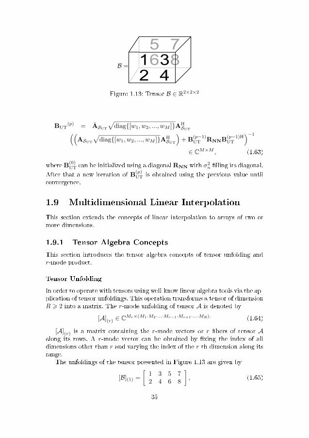
B = 1

2

3

4

5

6

7

8

Figure 1.13: Tensor B ∈ R2×2×2

BUT(p) = ASUT

√diag{[w1, w2, ..., wM ]}AH

SUT((ASUT

√diag{[w1, w2, ..., wM ]}AH

SUT

)+ B

(p−1)UT RNNB

(p−1)HUT

)−1

∈ CM×M , (1.63)

where B(0)UT can be initialized using a diagonal RNN with σ2

n �lling its diagonal.

After that a new iteration of B(p)UT is obtained using the previous value until

convergence.

1.9 Multidimensional Linear Interpolation

This section extends the concepts of linear interpolation to arrays of two ormore dimensions.

1.9.1 Tensor Algebra Concepts

This section introduces the tensor algebra concepts of tensor unfolding andr-mode product.

Tensor Unfolding

In order to operate with tensors using well-know linear algebra tools via the ap-plication of tensor unfoldings. This operation transforms a tensor of dimensionR > 2 into a matrix. The r-mode unfolding of tensor A is denoted by

[A](r) ∈ CMr×(M1·M2·...·Mr−1·Mr+1·...·MR). (1.64)

[A](r) is a matrix containing the r-mode vectors or r �bers of tensor Aalong its rows. A r-mode vector can be obtained by �xing the index of alldimensions other than r and varying the index of the r-th dimension along itsrange.

The unfoldings of the tensor presented in Figure 1.13 are given by

[B](1) =

[1 3 5 72 4 6 8

], (1.65)

35

[B](2) =

[1 2 5 63 4 7 8

], (1.66)

[B](3) =

[1 2 3 45 6 7 8

]. (1.67)

r-Mode Product

The r-mode product of a tensor A ∈ CM1×M2×...×Mr and a matrix D ∈ CL×Mr

is denote byC = A×r D ∈ CM1×M2×...×L×...×Mr , (1.68)

which is equivalent to[A×r D] = D · [A](r). (1.69)

Thus, the matrix D must have the same number of columns as the numbersof elements in the r-th dimension of A.

1.9.2 Multidimensional Data Model

The data model consider d planar wavefronts are impinging on an antennaarray containing M1 × M2 × ... × MR elements. The signal received at them1,m2, . . .mR antenna at a given time snapshot t is given by

xm1,m2,...mR,t =

d∑i=1

γm1,m2,...mR,dsi[n]

R∏r=1

ej·(mr−1)·µ(r)i

+nm1,m2,...mR,n, (1.70)

where si[n] is the complex symbol transmitted by the i-th source at timesnapshot n, nm1,m2,...mR,t is the zero mean circularly symmetric (ZMCS) whitecomplex Gaussian noise present at antenna m1,m2, . . .mR at time snapshot n.

γm1,m2,...mR is an imperfection present at the antenna m1,m2, . . .mR. µ(r)i

represents the spatial frequency of the signal transmitted by the i-th sourceover the r-th dimension, note that the spatial frequency can be mapped intodi�erent parameters depending on the dimension. In case of spatial dimension,it is mapped into a direction of arrival, while for frequency and time dimensionsit can be mapper into time delay of arrival and Doppler shift, respectively.

For the received signal to have the PARAFAC structure its steering arraymust have a Khatri-Rao structure as follows. Let Mr be the size of the r-thdimension, and M =

∏Rr=1Mr. A steering vector a

(r)i containing the spatial

frequencies relate to the i-th source over the r-th dimension can be de�ned as

a(r)i =

[1 ej·µ

(r)i · · · e(Mr−1)·j·µ(r)

i

]T. (1.71)

36

Therefore, an array steering vector for the i-th source can be written as

ai = a(1)i ⊗ a

(2)i ⊗ . . .⊗ a

(r)i ∈ CM×1, (1.72)

while the array steering matrix for the r-th dimension can be constructed as

A(r) =[a

(r)1 ,a

(r)2 , . . . ,a

(r)d

]∈ CM×d. (1.73)

Finally, the total steering matrix of the d sources can be constructed in termsof Khatri-Rao products of all array steering matrices of all dimensions.

A = A(1) �A(2) � . . . �A(r) ∈ CM×d. (1.74)

For the tensor notation, a PARAFAC steering tensor for each of the d signalsources can be obtained by

Ai = a(1)i ◦ a

(2)i ◦ . . . ◦ a

(r)i ∈ CM1×M2×···×MR , (1.75)

where ◦ is the outer product. A total array steering tensor can be constructedby concatenating the individual steering tensor for each of the signal sourcesover the r + 1 dimension, as it follows

A =[A1|R+1A2|R+1 . . . |R+1Ad] ∈ CM1×M2×···×MR×d. (1.76)

The |r operator represents the concatenation operation over the r-th dimen-sion.

A non PARAFAC steering tensor can be written as

X = (A� G)×R ST +N ,∈ CM1×M2×...×MR×N , (1.77)

hereN ∈ CM1×M2×...×MR×N is the noise tensor and contains the noise samplesinterfering with the measurements, and G ∈ CM1×M2×···×MR×d is a tensorcontaining the antenna imperfections.

1.9.3 Multidimensional Interpolation

Array interpolation can be extended to the multidimensional case by consid-ering the multidimensional data model and rewriting (1.19) as

I ×1 A1 ×2 A2...×R AR = A×1 B1 ×2 B2...×R BR, (1.78)

where Ar is the desired array response for the r-th dimension and Br is thetransformation matrix for the r-th dimension given by

Br = [A](r)A†r, (1.79)

where (�)† stands for the Moore�Penrose pseudo-inverse. Note that in thiscase the original array A has no PARAFAC structure, while the array afterthe interpolation has the PARAFAC structure.

37

Similar to what is done in the matrix case, the power response is used tothe detect sectors for interpolation. The power response for dimension r isgiven by

P (µ(r)) =

∣∣∣∣∣w(r)H(µ(r))R(r)XXw(r)(µ(r))

w(r)H(µ(r))w(r)(µ(r))

∣∣∣∣∣ ∈ R, (1.80)

where (·)H is the conjugate hermitian and R(r)XX is the spatial covariance matrix

for dimension (r). R(r)XX is given by

R(r)XX =

Mr

N∏Ri=1Mi

[X ](r)[X ]H(r) ∈ CMr×Mr . (1.81)

Following the matrix approach, the output of (1.80) is scanned for K sec-

tors, and for each sector the respective lower bound l(r)k ∈ D∆ and upper

bound u(r)k ∈ D∆, where k = 1, . . . ,K, are de�ned done in the matrix case. If

K sectors are detected, a detected sector with bounds [l(r)k , u

(r)k ] is said to be

centred at

ck =

∣∣∣u(r)k − l

(r)k

∣∣∣2

D∆

∈ D∆, (1.82)

After the sectors are detected for each of the dimensions, they can be dis-cretized and a transformation can be calculated following the same steps pre-sented for the one dimensional case. After Br has been obtained for all thedimensions to be interpolated the received data can be transformed by

X ×1 B1 ×2 B2 . . .×R BR. (1.83)

The transformation also a�ects the noise component, leading to coloured noiseat the output. This requires some sort of prewhitening to be applied prior tosome DOA estimation algorithms. For prewhitening schemes, the reader mayrefer to [26] for the matrix case and [25] for the tensor case.

Depending on the structure chosen for the interpolated array many dif-ferent DOA estimation methods can be applied. Multidimensional ESPRITapproaches such as [48] or methods based on the PARAFAC decompositionsuch as [29], [28] can be used.

1.10 Nonlinear Array Interpolation

In this section two nonlinear alternatives to array interpolation, allowing theapplication of FBA and SPS in highly correlated signal scenarios, are pre-sented. Subsection 1.10.1 presents an interpolation approach based on theMARS regression method, allowing a model to be created expressing non-linear relationships between the true and the desired array response. Subsec-tion 1.10.2 shows an interpolation approach based on GRNNs, this approach

38

can be implemented in a parallel manner, making it a good candidate for ar-ray interpolation under real-time constraints. For the nonlinear approachessector selection and discretization can be perform identically to when linearapproaches are employed.

1.10.1 MARS based interpolation

This work proposes a nonlinear interpolation method based on the MARStechnique. The MARS regression approach is detailed in Appendix E. Theproposed interpolation approach builds a mapping that splits the real andimaginary parts of the response of each of the antennas of the array, that is,a total of 2M MARS models are built to interpolate the array response withrespect to the combined sector S. Based on (E.4) this mapping can be writtenas

∀ (θ, φ) ∈ S :

[<{a(θ, φ)}={a(θ, φ)}

]= f (a(θ, φ))

=

∑LR1`=1 c

R`,1F

R`,1 (<{a(θ, φ)})...∑LRM

`=1 cR`,MF

R`,M (<{a(θ, φ)})∑LI1

`=1 cI`,1F

I`,1 (={a(θ, φ)})...∑LIM

`=1 cI`,MF

I`,M (={a(θ, φ)})

, (1.84)

where cRlm and cIlm are the weighting constants, FRlm and F Ilm are the basis

functions and LRm and LIm are the number of functions and weighting constantsof each model. Furthermore, <{a(θ, φ)} and ={a(θ, φ)} denote the real andimaginary part of vector a(θ, φ), respectively. Based on (E.6) the generalizedcross-validation (GCV) for the backward pass (step used to reduce possibleover-�tting of the model) can be written as

<{GCV} =

1|S|∑

(θ,φ)∈S(<{a[m](θ, φ)} − fRm(a(θ, φ)))2

(1− LRm+pLRm−1

2

|S| )2

, (1.85)

={GCV} =

1|S|∑

(θ,φ)∈S(={a[m](θ, φ)} − f Im(a(θ, φ)))2

(1− LIm+pLIm−1

2

|S| )2

, (1.86)

where fRm and f Im are the real and imaginary part of the model for the m-thantenna, respectively. Both <{GCV} and <{GCV} are used to avoid over-�tting, that is, to reduce the complexity of the model created in order to avoid�tting of the noise or of measurement errors of the array response. a[m](θ, φ)

39

denotes the m-th element of the virtual array response. To use this approachin an real-time system the models can be built in an initialization step. Sectorsof interest for the application of the MARS interpolation can be selected anda model can be built and stored as a look-up table. The data received can beinterpolated snapshot-wise with[

<{x[n]}={x[n]}

]= f (x[n]) , (1.87)

where x[n] ∈ CM×1 is the n -th column of matrix X with n = 1, . . . , N .In some cases, the antenna array will have a response which is similar

enough to the desired response in some of its �eld of view so that a linearapproach yields good results. Thus, the MARS approach can be used only onportions of the �eld of view where the real response di�ers strongly from thedesired one.

The MARS approach is especially useful for arrays with a small number ofelements. For linear approaches, the degrees of freedom of the linear approachare limited by the number of antennas in the virtual array. It is possible toincrease the degrees of freedom by creating a virtual array with a larger num-ber of antennas, however, this will lead to a transformation matrix that isill-conditioned and results in a large bias in the DOA estimates. The MARSapproach, on the other hand, can build as many hinge functions and relation-ships between them as necessary.

1.10.2 GRNN based interpolation

GRNNs are a type of neural network used for general regression problems thatare extended in this work for the problem of array interpolation. An overviewof GRNNs is presented in Appendix F.

Classic interpolation relies on transforming an array response over the dis-crete set of angles S. In linear array interpolation, the choice of points thatbelong to S is usually an arbitrary one, based solely on the prede�ned sectorbounds and the chosen angular resolution. When applying a linear approach,angular resolution is usually chosen to be as high as possible, thus, the set ofpoints belonging to S is usually closely spaced. This is not necessary when ap-plying the GRNN since it is capable of interpolating between multiple sets oftraining data. In fact, a dense set of training points will result in an increasedcomputational load while providing very little bene�t to the overall accuracyof the GRNN based array interpolation.

The neural network representing the real and imaginary parts of the arraycan be built by extending (F.1) and (F.2) to the application at hand, resultingin the mapping [

<{x[n]}={x[n]}

]= f (x[n], a(θ, φ),a(θ, φ)) , (1.88)

40

and

<{x[m][n]} =

∑(θ,φ)∈S <{a[m](θ, φ)}e−

ξ(θ,φ)

2σ2∑(θ,φ)∈S e

− ξ(θ,φ)

2σ2

, (1.89)

={x[m][n]} =

∑(θ,φ)∈S ={a[m](θ, φ)}e−

ξ(θ,φ)

2σ2∑(θ,φ)∈S e

− ξ(θ,φ)

2σ2

, (1.90)

where σ2 is the smoothness parameter, and

ξ(θ, φ) = ||x[n]− a(θ, φ)||22. (1.91)

Once the data has been interpolated to the desired array structure, array signalprocessing schemes such as FBA, SPS or ESPRIT can be applied. Di�erently,from other array interpolation methods, there is no noise color introduced bythe interpolation, therefore pre-whitening is not necessary.

One of the advantages of applying GRNNs to array interpolation is thatthe sectors considered for transformation can be made very large while havinga small e�ect on the accuracy of the interpolation. As shown in (1.89, 1.90), incase the input resembles the data used for the training in a certain region ofthe transformed sector, this data will have a larger weight. On the other hand,if the input is distant from any region of the transformed sector, this regionwill have very little in�uence on the output of the interpolation.

Therefore, with a GRNN it is possible to transform very large regions of the�eld of view of the array without su�ering from the same problems as the onespresent in linear array interpolation, where the transformation error grows asthe transformed region grows. On the other hand, transforming a large regionusing the GRNN will increase the computational cost of the interpolation. Asshown in Figure F.1 it is possible to implement the proposed GRNN arrayinterpolation in a parallel manner, leading to a faster interpolation. Thus, theproposed GRNN array interpolation is a possible alternative for precise arrayinterpolation in real-time applications.

1.11 Numerical Simulation Results

This section presents a performance assessment of the proposed multidimen-sional linear approach in Subsection 1.11.1 and of the proposed adaptive linearand nonlinear approaches in Subsection 1.11.2.

1.11.1 Multidimensional Linear Performance Results

In order to study the performance of the proposed multidimensional methoda set of numerical simulations is performed. Three signals impinge on a 8× 8planar array. The spatial frequencies are set to (−π3 ,π3 ), (π5 ,π5 ) and (π3 ,−π3 ).

41

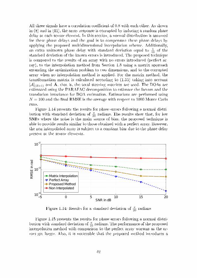
All three signals have a correlation coe�cient of 0.8 with each other. As shownin (8) and in (11), the array response is corrupted by inducing a random phasedelay at each sensor element. In this section, a normal distribution is assumedfor these phase delays and the goal is to compensate these phase delays byapplying the proposed multidimensional interpolation scheme. Additionally,an extra unknown phase delay with standard deviation equal to 1

10 of thestandard deviation of the known errors is introduced. The proposed techniqueis compared to the results of an array with no errors introduced (perfect ar-ray), to the interpolation method from Section 1.8 using a matrix approachextending the optimization problem to two dimensions, and to the corruptedarray when no interpolation method is applied. For the matrix method, thetransformation matrix is calculated according to (1.55) taking into account[A](R+1) and A, that is, the total steering matrices are used. The DOAs areestimated using the PARAFAC decomposition to estimate the factors and thetranslation invariance for DOA estimation. Estimations are performed usingN = 100 and the �nal RMSE is the average with respect to 1000 Monte Carloruns.

Figure 1.14 presents the results for phase errors following a normal distri-bution with standard deviation of π

20 radians. The results show that, for lowSNRs where the noise is the main source of bias, the proposed technique isable to provide results similar to those obtained with a perfect array. However,the non interpolated array is subject to a constant bias due to the phase delaypresent at the sensor elements.

−5 0 5 10 15 2010

−4

10−3

10−2

SNR in dB

RM

SE

in rad

Matrix Interpolation

Perfect Array

Proposed Method

Non Interpolated

Figure 1.14: Results for a standard deviation of π20 radians

Figure 1.15 presents the results for phase errors following a normal distri-bution with standard deviation of π

10 radians. The performance of the proposedinterpolation method with comparison to the perfect array worsens as the er-rors get larger. Also, it is noticeable that the proposed method introduces a

42

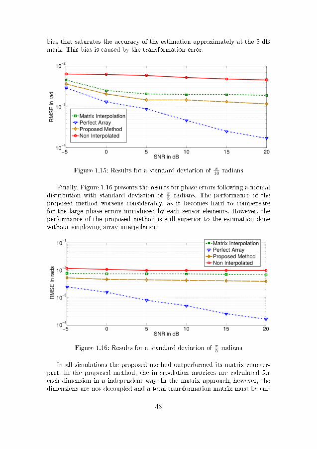
bias that saturates the accuracy of the estimation approximately at the 5 dBmark. This bias is caused by the transformation error.

−5 0 5 10 15 2010

−4

10−3

10−2

SNR in dB

RM

SE

inra

d

Matrix Interpolation

Perfect Array

Proposed Method

Non Interpolated

Figure 1.15: Results for a standard deviation of π10 radians

Finally, Figure 1.16 presents the results for phase errors following a normaldistribution with standard deviation of π

5 radians. The performance of theproposed method worsens considerably, as it becomes hard to compensatefor the large phase errors introduced by each sensor elements. However, theperformance of the proposed method is still superior to the estimation donewithout employing array interpolation.

−5 0 5 10 15 2010

−4

10−3

10−2

10−1

SNR in dB

RM

SE

in r

ads

Matrix Interpolation

Perfect Array

Proposed Method

Non Interpolated

Figure 1.16: Results for a standard deviation of π5 radians

In all simulations the proposed method outperformed its matrix counter-part. In the proposed method, the interpolation matrices are calculated foreach dimension in a independent way. In the matrix approach, however, thedimensions are not decoupled and a total transformation matrix must be cal-

43

culated taking into account all the permutations possible between angularresponses from each dimension. Thus, the calculation of this transformationmatrix is highly overdetermined resulting in a larger transformation error. An-other advantage of the proposed method is that the optimization problems areone dimensional, resulting in a smaller computational load.

1.11.2 Nonlinear Performance Results

The performance of the proposed algorithms is tested considering a manufac-tured 6×1 linear antenna array shown in Figure 1.17 [15]. The single antennasare circularly polarized dielectric resonator antennas (DRA) [14], exhibiting astrong miniaturization of the aperture. The antennas are tuned to work at GPSL1 frequency band centered around 1575.42 MHz in standalone con�guration.Once in the array, no attempt has been made to re-tune them, in order to em-phasize the mutual coupling e�ects and eventual degradation. This 6×1 lineararray was especially designed for research on mutual coupling with adjustableinter-element spacing of the 6 antennas. The small dimensions of the singleantennas allow to place them quite close to each other, up to a minimum dis-tance of 30 mm (≈ 0.16λ at L1 central frequency). The following simulationsconsider array responses of the manufactured array measured in an anechoicchamber as well as array responses simulated using a 3D electromagnetic sim-ulator (ANSYS HFSS). Thus, realistic assessment of the proposed algorithmscan be achieved considering measured and properly simulated array responses.

The simulations are performed considering the receiver has no previousknowledge of the received signal. The combined sector is detected and dis-cretized according to the methods presented in Section 1.7. After discretizationthe combined sector is interpolated using the linear and nonlinear methods pro-posed in Sections 1.7 and 1.10. The model order of the interpolated data thenis estimated by applying FBA and SPS adaptively and using RADOI [91] asthe model order estimation method following the procedure proposed in [72].Once model order is estimated the DOA estimates are obtained using TLS-ESPRIT [93].

For obtaining RXX N = 100 snapshots are used and the Root MeanSquared Error (RMSE) is calculated with respect to 1000 Monte Carlo simula-tions. Two signals from θ1 = 45◦ and θ2 = 15◦ with σ2

1 = σ22 = 1 and γ1,2 = 1

according to (1.4) are impinging on the array. The given RMSE is

RMSE =

√√√√ 1

K

K∑k=1

((θk1 − θ1)2 + (θk2 − θ2)2

), (1.92)

where θki is the estimate of θi at the k-th Monte Carlo run.The Signal-to-Noise-Ratio (SNR) is de�ned as

SNR =σ2

1

σ2n

=σ2

2

σ2n

= · · · = σ2d

σ2n

. (1.93)

44

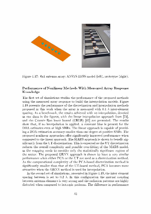
Figure 1.17: 6x1 antenna array: ANSYS HFSS model (left), prototype (right).

Performance of Nonlinear Methods With Measured Array ResponseKnowledge

The �rst set of simulations studies the performance of the proposed methodsusing the measured array response to build the interpolation models. Figure1.18 presents the performance of the discretization and interpolation methodsproposed in this work when the array is measured with 0.4 λ inter-elementspacing. As a benchmark, the results achieved with no interpolation, denotedas raw data in the �gures, with the linear interpolation approach from [72],and the Cramér�Rao lower bound (CRLB) [87] are presented. The resultsshow that, if no interpolation is applied, a constant bias is present for theDOA estimates even at high SNRs. The linear approach is capable of provid-ing a DOA estimation accuracy smaller than one degree at positive SNRs. Theproposed nonlinear approaches o�er signi�cantly improved performance whencompared to the linear approach. The MARS approach is shown to bene�t sig-ni�cantly from the UT discretization. This is expected as the UT discretizationreduces the overall complexity and possible over-�tting of the MARS model,as the mapping needs to consider only the statistically signi�cant regions ofthe sector. The proposed GRNN approach is shown to have a very similarperformance when either PCA or the UT are used as a discretization method.As the computational complexity of the PCA-based discretization method issigni�cantly smaller than that of the UT-based method, PCA becomes moreattractive when the GRNN method is used for interpolation.

In the second set of simulations, presented in Figure 1.19, the inter-elementspacing between is set to 0.2 λ. In this con�guration the mutual couplingbetween antenna elements is very strong and the radiation patterns are highlydistorted when compared to isotropic patterns. The di�erence in performance

45

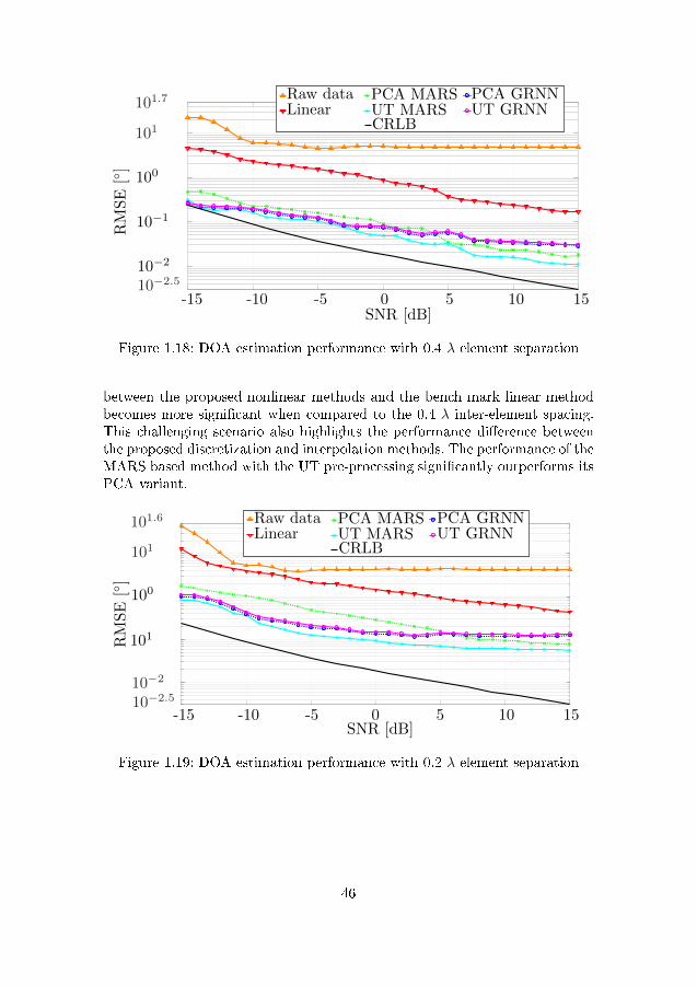
-15 -10 -5 0 5 10 15

10−2

10−1

Raw dataLinear

PCA MARSUT MARS

PCA GRNNUT GRNN

CRLB

100

101

SNR [dB]

RMSE

[◦]

101.7

10−2.5

Figure 1.18: DOA estimation performance with 0.4 λ element separation

between the proposed nonlinear methods and the bench mark linear methodbecomes more signi�cant when compared to the 0.4 λ inter-element spacing.This challenging scenario also highlights the performance di�erence betweenthe proposed discretization and interpolation methods. The performance of theMARS based method with the UT pre-processing signi�cantly outperforms itsPCA variant.

-15 -10 -5 0 5 10 15

Raw dataLinear

PCA MARSUT MARS

PCA GRNNUT GRNN

CRLB

10−2

101

100

101

RMSE

[◦]

SNR [dB]

101.6

10−2.5

Figure 1.19: DOA estimation performance with 0.2 λ element separation

46

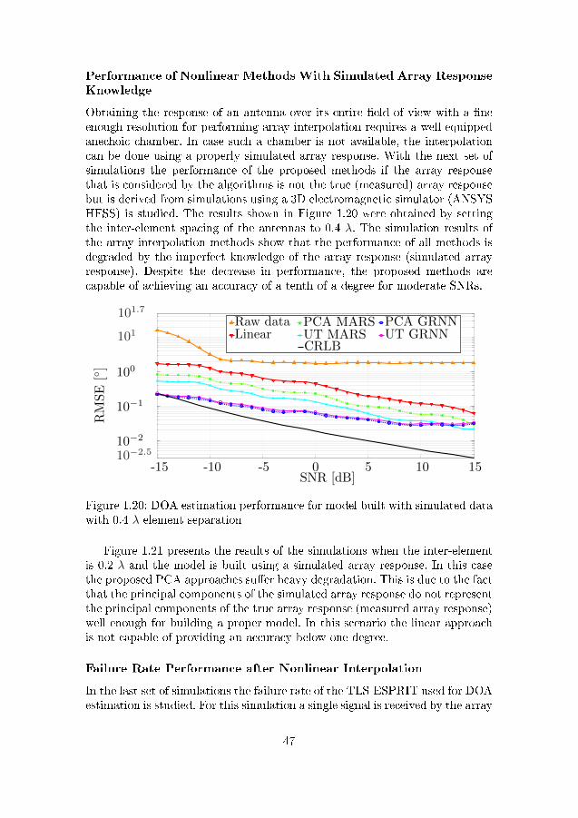
Performance of Nonlinear Methods With Simulated Array ResponseKnowledge

Obtaining the response of an antenna over its entire �eld of view with a �neenough resolution for performing array interpolation requires a well equippedanechoic chamber. In case such a chamber is not available, the interpolationcan be done using a properly simulated array response. With the next set ofsimulations the performance of the proposed methods if the array responsethat is considered by the algorithms is not the true (measured) array responsebut is derived from simulations using a 3D electromagnetic simulator (ANSYSHFSS) is studied. The results shown in Figure 1.20 were obtained by settingthe inter-element spacing of the antennas to 0.4 λ. The simulation results ofthe array interpolation methods show that the performance of all methods isdegraded by the imperfect knowledge of the array response (simulated arrayresponse). Despite the decrease in performance, the proposed methods arecapable of achieving an accuracy of a tenth of a degree for moderate SNRs.

-15 -10 -5 0 5 10 15

10−2

10−1

100

101

RMSE

[◦]

SNR [dB]

Raw dataLinear

PCA MARSUT MARS

PCA GRNNUT GRNN

CRLB

101.7

10−2.5

Figure 1.20: DOA estimation performance for model built with simulated datawith 0.4 λ element separation

Figure 1.21 presents the results of the simulations when the inter-elementis 0.2 λ and the model is built using a simulated array response. In this casethe proposed PCA approaches su�er heavy degradation. This is due to the factthat the principal components of the simulated array response do not representthe principal components of the true array response (measured array response)well enough for building a proper model. In this scenario the linear approachis not capable of providing an accuracy below one degree.

Failure Rate Performance after Nonlinear Interpolation

In the last set of simulations the failure rate of the TLS-ESPRIT used for DOAestimation is studied. For this simulation a single signal is received by the array

47

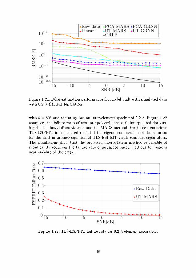
-15 -10 -5 0 5 10 15

10−2

10−1

100

101

RMSE

[◦]

SNR [dB]

Raw dataLinear

PCA MARSUT MARS

PCA GRNNUT GRNN

CRLB101.9

10−2.5

Figure 1.21: DOA estimation performance for model built with simulated datawith 0.2 λ element separation

with θ = 80◦ and the array has an inter-element spacing of 0.2 λ. Figure 1.22compares the failure rates of non-interpolated data with interpolated data us-ing the UT-based discretization and the MARS method. For these simulationsTLS-ESPRIT is considered to fail if the eigendecomposition of the solutionfor the shift invariance equation of TLS-ESPRIT yields complex eigenvalues.The simulations show that the proposed interpolation method is capable ofsigni�cantly reducing the failure rate of subspace based methods for regionsnear end-�re of the array.

-15 -10 -5 0 5 10 150

0.1

0.2

0.3

0.4

0.5

0.6

0.7

Raw Data

ESPRIT

Failure

Rate

UT MARS

SNR[dB]

Figure 1.22: TLS-ESPRIT failure rate for 0.2 λ element separation

48

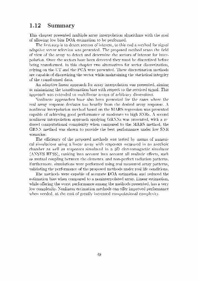
1.12 Summary

This chapter presented multiple array interpolation algorithms with the goalof allowing low bias DOA estimation to be performed.

The �rst step is to detect sectors of interest, to this end a method for signaladaptive sector selection was presented. The proposed method scans the �eldof view of the array to detect and determine the sectors of interest for inter-polation. Once the sectors have been detected they must be discretized beforebeing transformed, in this chapter two alternatives for sector discretization,relying on the UT and the PCA were presented. These discretization methodsare capable of discretizing the sector while maintaining the statistical integrityof the transformed data.

An adaptive linear approach for array interpolation was presented, aimingat minimizing the transformation bias with respect to the received signal. Thisapproach was extended to multilinear arrays of arbitrary dimensions.

Nonlinear approaches have also been presented for the cases where thereal array response deviates too heavily from the desired array response. Anonlinear interpolation method based on the MARS regression was presentedcapable of achieving good performance at moderate to high SNRs. A secondnonlinear interpolation approach applying GRNNs was presented, with a re-duced computational complexity when compared to the MARS method, theGRNN method was shown to provide the best performance under low SNRscenarios.

The e�ciency of the proposed methods was tested by means of numeri-cal simulations using a linear array with responses measured in an anechoicchamber as well as responses simulated in a 3D electromagnetic simulator(ANSYS HFSS), tanking into account into account all realistic e�ects, suchas mutual coupling between the elements, and non-perfect radiation patterns.Furthermore, simulations were performed using real measured array patterns,validating the performance of the proposed methods under real life conditions.

The methods were capable of accurate DOA estimation and reduced theestimation bias when compared to a noninterpolated array. Linear estimation,while o�ering the worst performance among the methods presented, has a verylow complexity. Nonlinear estimation methods can o�er improved performancewhen needed, at the cost of greatly increased computational complexity.

49

Chapter 2

Cooperative MIMO forWireless Sensor Networks

In this chapter the following research question is addressed:Can array processing techniques be used to provide improved lifetime and com-munication performance in wireless sensor network?

2.1 Overview and Contribution

The remainder of this section is organized as follows:

� Motivation: An introduction to wireless sensor networks and how thechallenges they face can be addressed using array processing is presentedin this section.

� Wireless Sensor Networks Organization: This section presents abrief description of the usual organization inside WSNs

� Cooperative MIMO: Here, the concept of Cooperative MIMO (C-MIMO) is detailed. The mathematical model behind MIMO is addressedand the steps involved in performing MIMO over a distributed set ofdevices are presented.

� Energy Analysis: In this section the energy consumption of single-hop,multi-hop and C-MIMO communications is studied. The threshold forwhen to switch between di�erent communication techniques is derivedto maximize the energy e�ciency with respect to the distance involvedin the communication.

� Synchronization: Here, the critical problem of synchronization for adistributed MIMO system is studied. The e�ects of synchronization er-rors in the performance of MIMO transmissions is analysed. Two di�erent

51

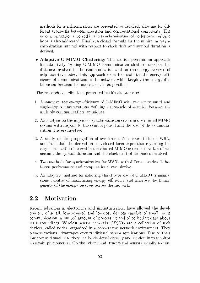
methods for synchronization are presented as detailed, allowing for dif-ferent trade-o�s between precision and computational complexity. Theerror propagation involved in the synchronization of nodes over multiplehops is also addressed. Finally, a closed formula for the minimum resyn-chronization interval with respect to clock drift and symbol duration isderived.

� Adaptive C-MIMO Clustering: This section presents an approachfor adaptively forming C-MIMO communication clusters based on thedistance involved in the communication and on the energy reserves ofneighbouring nodes. This approach seeks to maximize the energy e�-ciency of communications in the network while keeping the energy dis-tribution between the nodes as even as possible.

The research contributions presented in this chapter are:

1. A study on the energy e�ciency of C-MIMO with respect to multi andsingle-hop communications, de�ning a threshold of selection between themultiple communication techniques.

2. An analysis on the impact of synchronization errors in distributed MIMOsystem with respect to the symbol period and the size of the communi-cation clusters involved.

3. A study on the propagation of synchronization errors inside a WSN,and from that the derivation of a closed form expression regarding theresynchronization interval in distributed MIMO systems that takes intoaccount the symbol duration and the clock drift of the nodes involved.

4. Two methods for synchronization for WSNs with di�erent trade-o�s be-tween performance and computational complexity.

5. An adaptive method for selecting the cluster size of C-MIMO transmis-sions capable of maximizing energy e�ciency and improve the homo-geneity of the energy reserves across the network.

2.2 Motivation

Recent advances in electronics and miniaturization have allowed the devel-opment of small, low-powered and low-cost devices capable of small rangecommunication, a limited amount of processing and of collecting data aboutits surroundings. Wireless sensor networks (WSNs) are a collection of suchdevices, called nodes, organized in a cooperative network environment. Theypossess various advantages over traditional sensor applications. Due to theirlow cost and small size they can be deployed densely and randomly to monitora certain phenomenon. On the other hand, traditional sensors usually require

52

extensive planning in their deployment and, depending on the nature of thephenomenon to be sensed, cannot be placed near it due to their high cost.WSNs are usually self-contained and capable of organizing the network on the�y. Due to this characteristics, these networks are suitable for deployment onharsh environments.

WSN usage ranges from military applications, such as battle�eld surveil-lance and targeting, to healthcare applications, such as portable automateddrug infusion systems in hospitals [1]. However, the extensive use of WSNs isstill being hindered by the limited energy budget available in the nodes thatconstitute the networks. Furthermore, since WSNs are deployed even in harshand hard-to-reach environments, replacing individual nodes, or their batter-ies, is not always practical. Therefore, extensive research is being performedto maximize the energy e�ciency of WSNs [34].

Solutions for minimizing energy consumption in WSNs have been proposedthrough di�erent layers by analyzing energy e�ciency for all the tasks in-volved in WSNs. Given that communication is the most energy consumingtask, diminishing the need for communication and increasing the e�ciency ofcommunication are the promising directions to achieve WSNs with longer life-time [82]. While many proposals focus on enhancing energy e�ciency in thenetwork layer using energy e�cient routing protocols [44, 50], some focus onenhancing the communication e�ciency by proposing energy e�cient proto-cols for medium access control (e.g., [18,66]). Other proposals consider energyaware processing approaches for communication among sensor nodes in WSNs,as presented in [107], as well as the application of alternative solutions withinthe physical layer [97,98].

Multi-hop communication is a widely used technique to obtain improvedenergy e�ciency and to maximize network lifetime by spreading energy con-sumption over di�erent nodes [17]. Multi-hop techniques take advantage of thecooperative nature of WSNs in splitting the distance involved in communica-tion by employing intermediary nodes to forward data packets. Since free spaceloss is not linear, splitting the distance by using intermediary nodes results inreduced power demand, thus minimizing transmission energy consumption.

Another proposal made by taking advantage of the cooperative nature ofWSNs is the formation of cooperative Multiple-Input Multiple-Output (C-MIMO) clusters [23]. The faster data transmission rates achievable with C-MIMO system allow for interaction between fast-moving mobile nodes andtraditional static ones [76,77]. C-MIMO also allows the application of antennaarray techniques such as beamforming or DOA estimation. The usage of C-MIMO results in reduced hardware complexity on single nodes as it is notnecessary to employ multiple antennas and radios at a single node. Thus, it ispossible to use C-MIMO with no modi�cations to the hardware of existing sen-sor nodes. The complexity is transferred to the software, which is responsiblefor managing the communication involving a large number of nodes.

53

Keeping in view the characteristics and advantages of C-MIMO, a num-ber of problems that come in the way of e�ectively implementing C-MIMOin WSNs are studied in this thesis and solutions are proposed. The proposedsolutions deal with problems that may arise when implementing C-MIMO inWSNs, such as time synchronizing of sensor nodes, routing for C-MIMO com-munication, adaptively forming C-MIMO clusters and analyzing the energy ef-�ciency of C-MIMO. This work aims at fostering implementation of C-MIMOfor di�erent applications and presenting a performance analysis of C-MIMOfor WSNs, considering relevant technical aspects. Furthermore, the energy ef-�ciency of a C-MIMO network, operating on top of the proposed framework,is studied based on realistic node speci�cations.

2.3 Wireless Sensor Networks Organization

WSNs are at their very principle decentralized, ad hoc and self containedsystems. Decentralization, however, does not imply a lack of organization inWSNs, it refers only to the capacity of the network to function properly inthe event that any of its components cease to function, i.e, the network doesnot depend on a single speci�c element to work. The ad hoc capability impliesthat a new element can join the network and operate on it without any priorcon�guration. Being self-contained means that wireless sensor networks do notrely on any external system to operate.

With these three characteristics in mind, an analysis can be made on theusual methods of organizing a WSN. These methods are usually divided intotwo categories, a peer-to-peer or planar architecture and a cluster based orhierarchical architecture.

In peer-to-peer networks there exists no distinction or separation betweenmembers, they often possess exactly the same capabilities and resources. Thisvery loose environment distances itself from usual network organizations andprovides a more homogenous and locally autonomous framework. Peer-to-peernetwork members interact with each other to share more than informationbut also all available resources such as processing power and storage capacity.However, the lack of any "leader" element also means that the task of makingdecisions as simple as allocating IP addresses to new members can be quitecomplex.

Cluster based networks, on the other hand, are closer to the conventionalnetwork architectures. In cluster based networks the elements are usually di-vided into two categories: Full Function Devices (FFD) and Reduced FunctionDevices (RFD). RFDs are elements with limited resources, usually only pos-sessing a sensing element, a radio for wireless communication and the process-ing power necessary only to perform the said sensing and forwarding of thiscaptured information. FFDs are more powerful elements, they are responsiblefor organizing clusters of RFDs, routing and repeating information across thenetwork as well as performing in any network processing necessary, the sen-

54

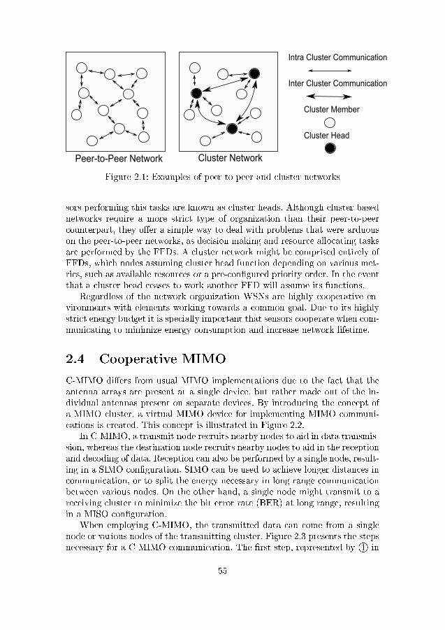
Peer-to-Peer Network Cluster Network

Intra Cluster Communication

Inter Cluster Communication

Cluster Member

Cluster Head

Figure 2.1: Examples of peer-to-peer and cluster networks

sors performing this tasks are known as cluster heads. Although cluster basednetworks require a more strict type of organization than their peer-to-peercounterpart, they o�er a simple way to deal with problems that were arduouson the peer-to-peer networks, as decision making and resource allocating tasksare performed by the FFDs. A cluster network might be comprised entirely ofFFDs, which nodes assuming cluster head function depending on various met-rics, such as available resources or a pre-con�gured priority order. In the eventthat a cluster head ceases to work another FFD will assume its functions.

Regardless of the network organization WSNs are highly cooperative en-vironments with elements working towards a common goal. Due to its highlystrict energy budget it is specially important that sensors cooperate when com-municating to minimize energy consumption and increase network lifetime.

2.4 Cooperative MIMO

C-MIMO di�ers from usual MIMO implementations due to the fact that theantenna arrays are present at a single device, but rather made out of the in-dividual antennas present on separate devices. By introducing the concept ofa MIMO cluster, a virtual MIMO device for implementing MIMO communi-cations is created. This concept is illustrated in Figure 2.2.

In C-MIMO, a transmit node recruits nearby nodes to aid in data transmis-sion, whereas the destination node recruits nearby nodes to aid in the receptionand decoding of data. Reception can also be performed by a single node, result-ing in a SIMO con�guration. SIMO can be used to achieve longer distances incommunication, or to split the energy necessary in long range communicationbetween various nodes. On the other hand, a single node might transmit to areceiving cluster to minimize the bit error rate (BER) at long range, resultingin a MISO con�guration.

When employing C-MIMO, the transmitted data can come from a singlenode or various nodes of the transmitting cluster. Figure 2.3 presents the stepsnecessary for a C-MIMO communication. The �rst step, represented by 1O in

55

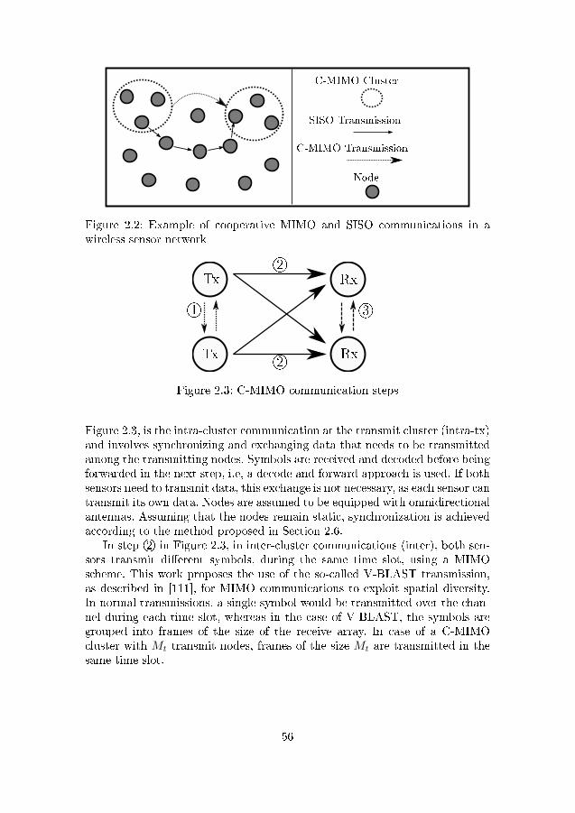
C-MIMO Cluster

SISO Transmission

C-MIMO Transmission

Node

Figure 2.2: Example of cooperative MIMO and SISO communications in awireless sensor network

1O

Tx

Tx

Rx

Rx2O

2O

3O

Figure 2.3: C-MIMO communication steps

Figure 2.3, is the intra-cluster communication at the transmit cluster (intra-tx)and involves synchronizing and exchanging data that needs to be transmittedamong the transmitting nodes. Symbols are received and decoded before beingforwarded in the next step, i.e, a decode and forward approach is used. If bothsensors need to transmit data, this exchange is not necessary, as each sensor cantransmit its own data. Nodes are assumed to be equipped with omnidirectionalantennas. Assuming that the nodes remain static, synchronization is achievedaccording to the method proposed in Section 2.6.

In step 2O in Figure 2.3, in inter-cluster communications (inter), both sen-sors transmit di�erent symbols, during the same time slot, using a MIMOscheme. This work proposes the use of the so-called V-BLAST transmission,as described in [111], for MIMO communications to exploit spatial diversity.In normal transmissions, a single symbol would be transmitted over the chan-nel during each time slot, whereas in the case of V-BLAST, the symbols aregrouped into frames of the size of the receive array. In case of a C-MIMOcluster with Mt transmit nodes, frames of the size Mt are transmitted in thesame time slot.

56

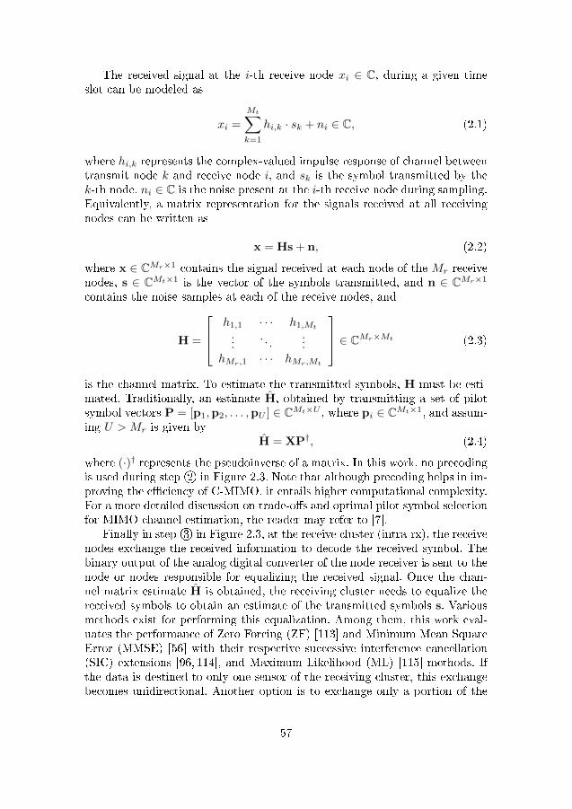
The received signal at the i-th receive node xi ∈ C, during a given timeslot can be modeled as

xi =

Mt∑k=1

hi,k · sk + ni ∈ C, (2.1)

where hi,k represents the complex-valued impulse response of channel betweentransmit node k and receive node i, and sk is the symbol transmitted by thek-th node. ni ∈ C is the noise present at the i-th receive node during sampling.Equivalently, a matrix representation for the signals received at all receivingnodes can be written as

x = Hs + n, (2.2)

where x ∈ CMr×1 contains the signal received at each node of the Mr receivenodes, s ∈ CMt×1 is the vector of the symbols transmitted, and n ∈ CMr×1

contains the noise samples at each of the receive nodes, and

H =

h1,1 · · · h1,Mt

.... . .

...hMr,1 · · · hMr,Mt

∈ CMr×Mt (2.3)

is the channel matrix. To estimate the transmitted symbols, H must be esti-mated. Traditionally, an estimate H, obtained by transmitting a set of pilotsymbol vectors P = [p1,p2, . . . ,pU ] ∈ CMt×U , where pi ∈ CMt×1, and assum-ing U > Mr is given by

H = XP†, (2.4)

where (·)† represents the pseudoinverse of a matrix. In this work, no precodingis used during step 2O in Figure 2.3. Note that although precoding helps in im-proving the e�ciency of C-MIMO, it entails higher computational complexity.For a more detailed discussion on trade-o�s and optimal pilot symbol selectionfor MIMO channel estimation, the reader may refer to [7].

Finally in step 3O in Figure 2.3, at the receive cluster (intra-rx), the receivenodes exchange the received information to decode the received symbol. Thebinary output of the analog digital converter of the node receiver is sent to thenode or nodes responsible for equalizing the received signal. Once the chan-nel matrix estimate H is obtained, the receiving cluster needs to equalize thereceived symbols to obtain an estimate of the transmitted symbols s. Variousmethods exist for performing this equalization. Among them, this work eval-uates the performance of Zero Forcing (ZF) [113] and Minimum Mean SquareError (MMSE) [56] with their respective successive interference cancellation(SIC) extensions [96, 114], and Maximum Likelihood (ML) [115] methods. Ifthe data is destined to only one sensor of the receiving cluster, this exchangebecomes unidirectional. Another option is to exchange only a portion of the

57

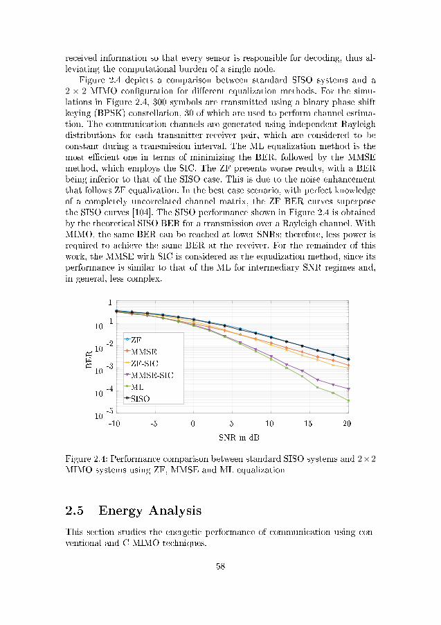
received information so that every sensor is responsible for decoding, thus al-leviating the computational burden of a single node.

Figure 2.4 depicts a comparison between standard SISO systems and a2 × 2 MIMO con�guration for di�erent equalization methods. For the simu-lations in Figure 2.4, 300 symbols are transmitted using a binary phase shiftkeying (BPSK) constellation, 30 of which are used to perform channel estima-tion. The communication channels are generated using independent Rayleighdistributions for each transmitter-receiver pair, which are considered to beconstant during a transmission interval. The ML equalization method is themost e�cient one in terms of minimizing the BER, followed by the MMSEmethod, which employs the SIC. The ZF presents worse results, with a BERbeing inferior to that of the SISO case. This is due to the noise enhancementthat follows ZF equalization. In the best case scenario, with perfect knowledgeof a completely uncorrelated channel matrix, the ZF BER curves superposethe SISO curves [104]. The SISO performance shown in Figure 2.4 is obtainedby the theoretical SISO BER for a transmission over a Rayleigh channel. WithMIMO, the same BER can be reached at lower SNRs; therefore, less power isrequired to achieve the same BER at the receiver. For the remainder of thiswork, the MMSE with SIC is considered as the equalization method, since itsperformance is similar to that of the ML for intermediary SNR regimes and,in general, less complex.

SNR in dB

-10 -5 0 5 10 15 20

BER

10-5

10-4

10-3

10-2

10-1

1

ZF

MMSE

ZF-SIC

MMSE-SIC

ML

SISO

Figure 2.4: Performance comparison between standard SISO systems and 2×2MIMO systems using ZF, MMSE and ML equalization

2.5 Energy Analysis

This section studies the energetic performance of communication using con-ventional and C-MIMO techniques.

58

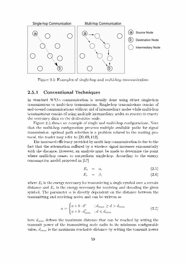
a

b

a

b

Single-hop Communication Multi-hop Communication

a

b

Source Node

Destination Node

Intermediary Node

Figure 2.5: Examples of single-hop and multi-hop communication

2.5.1 Conventional Techniques

In standard WSNs communication is usually done using either single-hoptransmissions or multi-hop transmissions. Single-hop transmissions consist ofend-to-end communications without aid of intermediary nodes while multi-hoptransmissions consist of using multiple intermediary nodes as routers to conveythe necessary data to the destination node.

Figure 2.5 shows an example of single and multi-hop con�gurations. Notethat the multi-hop con�guration presents multiple available paths for signaltransmission, optimal path selection is a problem related to the routing pro-tocol, the reader may refer to [20,69,112].

The increased e�ciency provided by multi-hop communication is due to thefact that the attenuation su�ered by a wireless signal increases exponentiallywith the distance. However, an analysis must be made to determine the pointwhere multi-hop ceases to outperform single-hop. According to the energyconsumption model proposed in [17]

Et = α, (2.5)

Er = β, (2.6)

where Et is the energy necessary for transmitting a single symbol over a certaindistance and Er is the energy necessary for receiving and decoding the givensymbol. The parameter α is directly dependent on the distance between thetransmitting and receiving nodes and can be written as

α =

{a+ b · dγ ; dmax ≥ d > dmin

a+ b · dγmin ; d 6 dmin(2.7)

here dmin de�nes the maximum distance that can be reached by setting thetransmit power of the transmitting node radio to its minimum con�gurablevalue, dmax is the maximum reachable distance by setting the transmit power

59

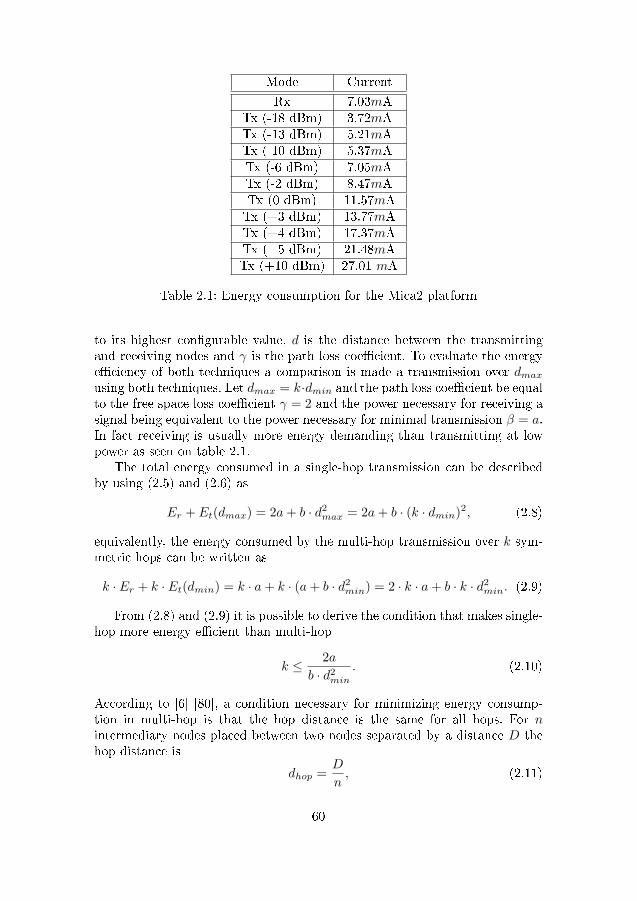
Mode Current

Rx 7.03mATx (-18 dBm) 3.72mATx (-13 dBm) 5.21mATx (-10 dBm) 5.37mATx (-6 dBm) 7.05mATx (-2 dBm) 8.47mATx (0 dBm) 11.57mATx (+3 dBm) 13.77mATx (+4 dBm) 17.37mATx (+5 dBm) 21.48mATx (+10 dBm) 27.01 mA

Table 2.1: Energy consumption for the Mica2 platform

to its highest con�gurable value, d is the distance between the transmittingand receiving nodes and γ is the path loss coe�cient. To evaluate the energye�ciency of both techniques a comparison is made a transmission over dmaxusing both techniques. Let dmax = k·dmin and the path loss coe�cient be equalto the free space loss coe�cient γ = 2 and the power necessary for receiving asignal being equivalent to the power necessary for minimal transmission β = a.In fact receiving is usually more energy demanding than transmitting at lowpower as seen on table 2.1.

The total energy consumed in a single-hop transmission can be describedby using (2.5) and (2.6) as

Er + Et(dmax) = 2a+ b · d2max = 2a+ b · (k · dmin)2, (2.8)

equivalently, the energy consumed by the multi-hop transmission over k sym-metric hops can be written as

k · Er + k · Et(dmin) = k · a+ k · (a+ b · d2min) = 2 · k · a+ b · k · d2

min. (2.9)

From (2.8) and (2.9) it is possible to derive the condition that makes single-hop more energy e�cient than multi-hop

k ≤ 2a

b · d2min

. (2.10)

According to [6] [80], a condition necessary for minimizing energy consump-tion in multi-hop is that the hop distance is the same for all hops. For nintermediary nodes placed between two nodes separated by a distance D thehop distance is

dhop =D

n, (2.11)

60

replacing dmin with dhop in (2.9) and taking its derivative with respect ton, the number of hops that minimizes the energy consumption in multi-hopcommunications can be found

nopt =

√b

2a·D. (2.12)

By replacing n by nopt in (2.11) the optimum hop distance in terms of energyconsumption can be written as

dchar =

√2a

b, (2.13)

where dchar is known as the characteristic distance. Note that dchar dependsonly upon the values of a and b, thus it is a parameter intrinsic to the sensorin question.

Care must be taken when employing the multi-hop approach to avoid re-ducing energy e�ciency by using an unnecessary number of hops. When ade-quately employed the multi-hop approach can lead to signi�cant energy savingin WSNs. However, multi-hopping su�ers from some serious disadvantages.Data forwarding is usually done on a best e�ort delivery basis. That meansthat the transmitting node has no guarantee of the transmitted data reachingits destination, or that it will be delivered within a given time frame. Multi-hop networking can lead to data congestion on nodes that are located betweennode clusters that generate heavy tra�c. This heavy tra�c will also result in ahigh drain of energy resources the in the nodes responsible for forwarding thedata. This will result in a high delivery delay and will eventually lead to de-pletion of energy in these midway nodes, resulting in a disconnected network.Data relaying is usually done in a decode and forward fashion, this can resultin a high delay even when there is no network congestion present.

Single-hop transmissions are not a�ected by network congestion as they areend-to-end communications, but they require a very high signal power whenemployed over large distances. If a single sensor is responsible for producinga large amount of data that needs to be transmitted over a large distance,this will lead to a very fast depletion of its energy resources. This unevendepletion is highly prejudicial to WSN operation, since replacing individualnodes might be as costly as replacing the entire network. Furthermore, single-hop transmissions might be unattainable over large distances due to the limitedpower at which sensor radios usually operate.

2.5.2 Cooperative MIMO

By introducing the C-MIMO approach, the drawbacks of the multi-hop ap-proach, such as larger delay and possible uneven energy consumption, can beavoided while still achieving energy e�cient communications. With the funda-mentals of C-MIMO reviewed in Section 2.4, a reliable, low BER and energy

61

e�cient communication can be implemented by taking advantage of the coop-erative nature of WSNs.

With the steps of Figure 2.3 in mind, it is possible to derive an analyticalexpression for the energy consumption of C-MIMO. De�ning Eintra as theenergy necessary to transmit an entire data packet to another sensor locatedwithin the C-MIMO cluster frontier, shown as 1O and 3O in Figure 2.3, theenergy spent on spreading the packet for transmission and for consolidating itfor equalization and decoding is given by

Etxintratx=Mt − 1

MtEintra, (2.14)

Etxintrarx=Mr − 1

MrEintra, (2.15)

respectively. For an Mt × Mr C-MIMO transmission, a central node thatspreads its packet to neighboring nodes needs to perform Mt − 1 transmis-sions with a cost of Eintra

Mt, as the packet is split into Mt smaller packets for

C-MIMO transmission. The same applies to consolidating the packet on thereceiving C-MIMO cluster, where Mr − 1 transmissions with a cost of Eintra

Mr,

are sent to a central node for equalization and decoding.Dissemination and consolidation of packets on the C-MIMO clusters also

consume signi�cant energy on the radios listening to the transmissions. There-fore, Mt − 1 receptions with a cost of Erx

Mt, where Erx is the energy cost for

receiving an entire data packet, are necessary at the transmitting cluster. Atthe receiving cluster, Mr − 1 receptions with a cost of Erx

Mrare necessary when

the received symbols are transmitted to the central node for decoding. Thus,the energy spent with receptions at the transmitting and receiver clusters isgiven by

Erxintratx=

(Mt − 1)

MtErx, (2.16)

Erxintrarx=

(Mr − 1)

MrErx, (2.17)

respectively. Additionally, as the packet is transmitting over long distancesusing C-MIMO, the Mr receiving nodes must listen. Therefore, another Mr

receptions with Erx

Mrcost are necessary.

Finally, Etxinteris the energy spent on transmitting a data packet, using

higher power for the long distance transmission step 2O on Figure 2.3. Mt

nodes transmit 1Mt

of the data packet.The total cost for transmitting a packet, using cooperative MIMO, is then

given by

EC-MIMO = Etxinter + Etxintratx+ Etxintrarx

+Erxintratx+ Erxintrarx

+ Erx. (2.18)

62

C-MIMO is capable of reaching large distances without demanding muchpower from a single node. In addition, since multiple copies of the same signalare received, the BER is considerably smaller at the same SNR. This makesthe C-MIMO capable of reaching long distances, using much less power thanSISO con�gurations do. C-MIMO con�gurations can lead to even lower BERratios, which allow even less power to be used for long range transmissions.

Next, assuming a multihop communication where the nodes involved areuniformly spaced and the energy necessary to transmit a data packet to thenext node is equivalent to the energy necessary to transmit inside a C-MIMOcluster, Eintra, the energy used for a multihop transmission is given by

Emhop = k (Eintra + Erx) , (2.19)

where k is the number of hops necessary to reach the destination node. From(2.18) and (2.19), the condition under which C-MIMO becomes more e�cientthan multihop, i.e. EC−MIMO < Emhop, is

Einter <

(k −

(Mt − 1

Mt+Mr − 1

Mr

))Eintra

+

(k −

(Mt − 1

Mt+Mr − 1

Mr+ 1

))Erx. (2.20)

From (2.20), it is clear that C-MIMO is more e�cient than multihop onlywhen the nodes are separated by a large number of hops.

Figure 2.4 shows that a BER of 10−3 can be reached using MIMO com-munication with SNR 8 dB lower than standard SISO communication. Fromthe speci�cations of the Harvard Mica2 platform [99], switching from 4 dBmtransmission to -15 dBm transmission means that the radio consumes approx-imately half of the energy to achieve the same BER.

Table 2.2 presents a comparison of the amounts of energy consumed by thedi�erent communication methods, namely, single-hop, multi-hop, and 2 × 2C-MIMO. When communicating with a node located 210 m away from theoriginating node, C-MIMO performs only slightly better than the single-hopand worse than the multi-hop approach. Even though the di�erence in perfor-mance between MIMO and single-hop is marginal, the energy consumption isspread out among various nodes when using the C-MIMO. Such a characteris-tic is highly desirable in WSNs. For longer distances, when using multi-hop, asthe increasing number of receptions starts becoming highly energy-demanding,C-MIMO outperforms multi-hop. From Table 2.2 the increased e�ciency pro-vided by the C-MIMO over large distances can be observed.

Note, that the computational complexity required in C-MIMO is higherthan that required in a standard SISO communication. However, the energyconsumed due to additional computational complexity is signi�cantly smallerthan the energy saved by e�cient communication. As a rule of thumb, in astandard communication, the energy spent in processing is 103 to 104 timesless than the energy spent in communication [2].

63

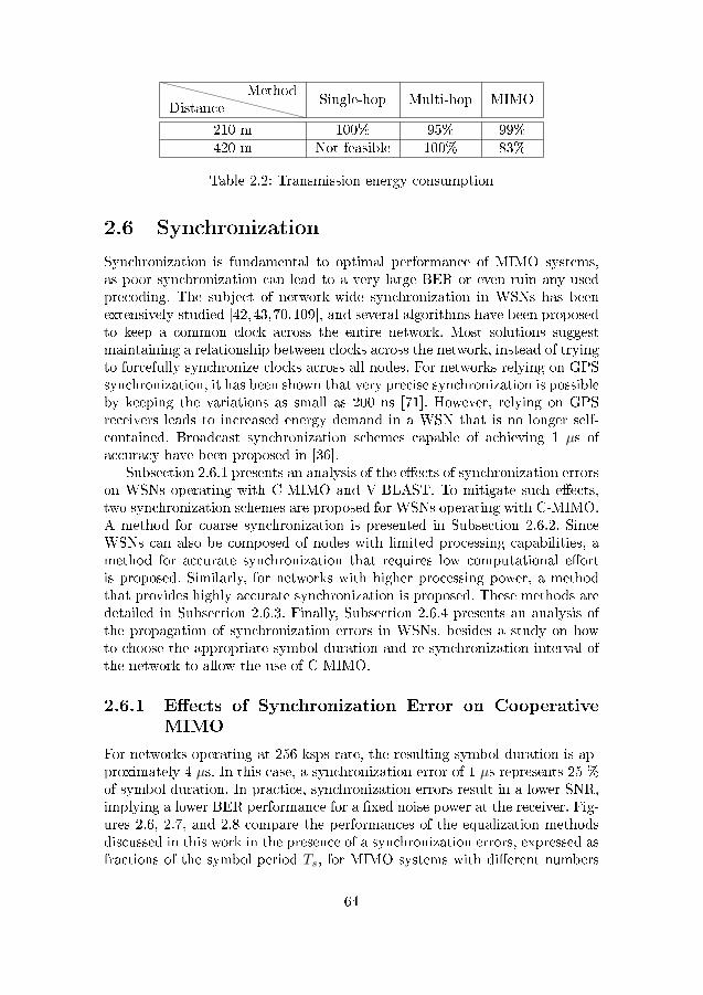
DistanceMethod

Single-hop Multi-hop MIMO

210 m 100% 95% 99%420 m Not feasible 100% 83%

Table 2.2: Transmission energy consumption

2.6 Synchronization

Synchronization is fundamental to optimal performance of MIMO systems,as poor synchronization can lead to a very large BER or even ruin any usedprecoding. The subject of network-wide synchronization in WSNs has beenextensively studied [42,43,70,109], and several algorithms have been proposedto keep a common clock across the entire network. Most solutions suggestmaintaining a relationship between clocks across the network, instead of tryingto forcefully synchronize clocks across all nodes. For networks relying on GPSsynchronization, it has been shown that very precise synchronization is possibleby keeping the variations as small as 200 ns [71]. However, relying on GPSreceivers leads to increased energy demand in a WSN that is no longer self-contained. Broadcast synchronization schemes capable of achieving 1 µs ofaccuracy have been proposed in [36].

Subsection 2.6.1 presents an analysis of the e�ects of synchronization errorson WSNs operating with C-MIMO and V-BLAST. To mitigate such e�ects,two synchronization schemes are proposed for WSNs operating with C-MIMO.A method for coarse synchronization is presented in Subsection 2.6.2. SinceWSNs can also be composed of nodes with limited processing capabilities, amethod for accurate synchronization that requires low computational e�ortis proposed. Similarly, for networks with higher processing power, a methodthat provides highly accurate synchronization is proposed. These methods aredetailed in Subsection 2.6.3. Finally, Subsection 2.6.4 presents an analysis ofthe propagation of synchronization errors in WSNs, besides a study on howto choose the appropriate symbol duration and re-synchronization interval ofthe network to allow the use of C-MIMO.

2.6.1 E�ects of Synchronization Error on CooperativeMIMO

For networks operating at 256 ksps rate, the resulting symbol duration is ap-proximately 4 µs. In this case, a synchronization error of 1 µs represents 25 %of symbol duration. In practice, synchronization errors result in a lower SNR,implying a lower BER performance for a �xed noise power at the receiver. Fig-ures 2.6, 2.7, and 2.8 compare the performances of the equalization methodsdiscussed in this work in the presence of a synchronization errors, expressed asfractions of the symbol period Ts, for MIMO systems with di�erent numbers

64

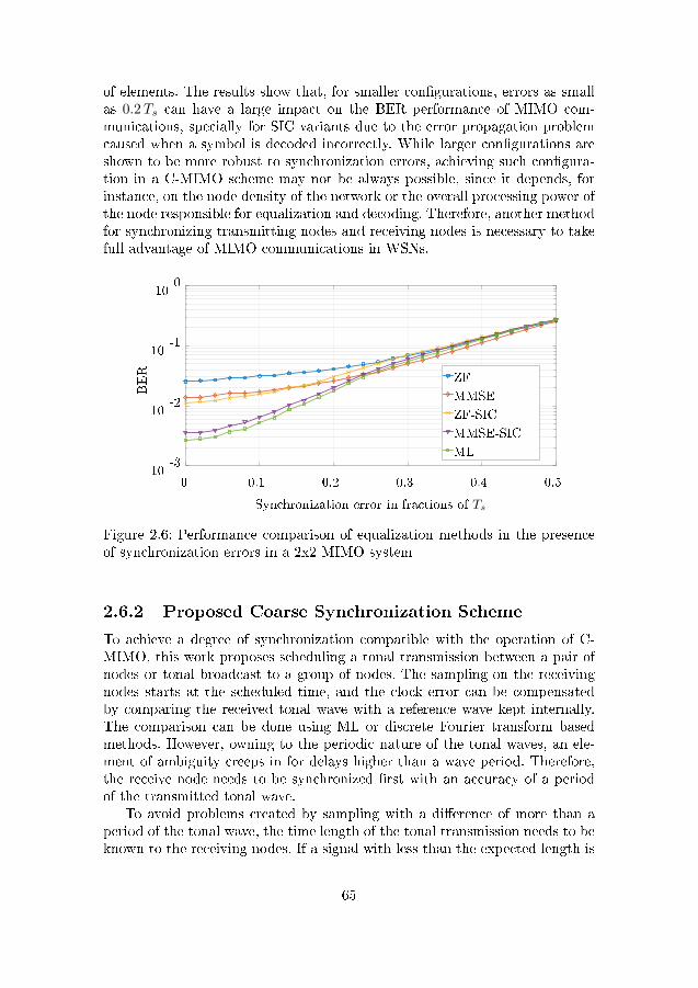
of elements. The results show that, for smaller con�gurations, errors as smallas 0.2Ts can have a large impact on the BER performance of MIMO com-munications, specially for SIC variants due to the error propagation problemcaused when a symbol is decoded incorrectly. While larger con�gurations areshown to be more robust to synchronization errors, achieving such con�gura-tion in a C-MIMO scheme may not be always possible, since it depends, forinstance, on the node density of the network or the overall processing power ofthe node responsible for equalization and decoding. Therefore, another methodfor synchronizing transmitting nodes and receiving nodes is necessary to takefull advantage of MIMO communications in WSNs.

Synchronization error in fractions of Ts

0 0.1 0.2 0.3 0.4 0.5

BER

10-3

10-2

10-1

100

ZF

MMSE

ZF-SIC

MMSE-SIC

ML

Figure 2.6: Performance comparison of equalization methods in the presenceof synchronization errors in a 2x2 MIMO system

2.6.2 Proposed Coarse Synchronization Scheme

To achieve a degree of synchronization compatible with the operation of C-MIMO, this work proposes scheduling a tonal transmission between a pair ofnodes or tonal broadcast to a group of nodes. The sampling on the receivingnodes starts at the scheduled time, and the clock error can be compensatedby comparing the received tonal wave with a reference wave kept internally.The comparison can be done using ML or discrete Fourier transform basedmethods. However, owning to the periodic nature of the tonal waves, an ele-ment of ambiguity creeps in for delays higher than a wave period. Therefore,the receive node needs to be synchronized �rst with an accuracy of a periodof the transmitted tonal wave.

To avoid problems created by sampling with a di�erence of more than aperiod of the tonal wave, the time length of the tonal transmission needs to beknown to the receiving nodes. If a signal with less than the expected length is

65

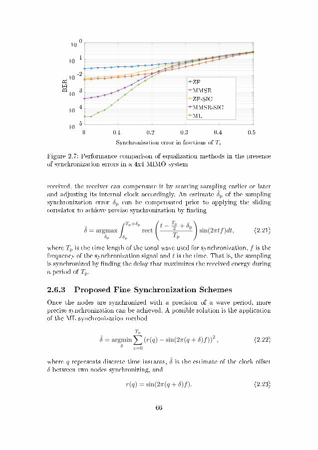
Synchronization error in fractions of Ts

0 0.1 0.2 0.3 0.4 0.5

BER

10-5

10-4

10-3

10-2

10-1

100

ZF

MMSE

ZF-SIC

MMSE-SIC

ML

Figure 2.7: Performance comparison of equalization methods in the presenceof synchronization errors in a 4x4 MIMO system

received, the receiver can compensate it by starting sampling earlier or laterand adjusting its internal clock accordingly. An estimate δp of the samplingsynchronization error δp can be compensated prior to applying the slidingcorrelator to achieve precise synchronization by �nding

δ = argmaxδp

∫ Tp+δp

δp

rect

(t− Tp

2 + δp

Tp

)sin(2πtf)dt, (2.21)

where Tp is the time length of the tonal wave used for synchronization, f is thefrequency of the synchronization signal and t is the time. That is, the samplingis synchronized by �nding the delay that maximizes the received energy duringa period of Tp.

2.6.3 Proposed Fine Synchronization Schemes

Once the nodes are synchronized with a precision of a wave period, moreprecise synchronization can be achieved. A possible solution is the applicationof the ML synchronization method

δ = argminδ

Tp∑z=0

(r(q)− sin(2π(q + δ)f))2, (2.22)

where q represents discrete time instants, δ is the estimate of the clock o�setδ between two nodes synchronizing, and

r(q) = sin(2π(q + δ)f). (2.23)

66

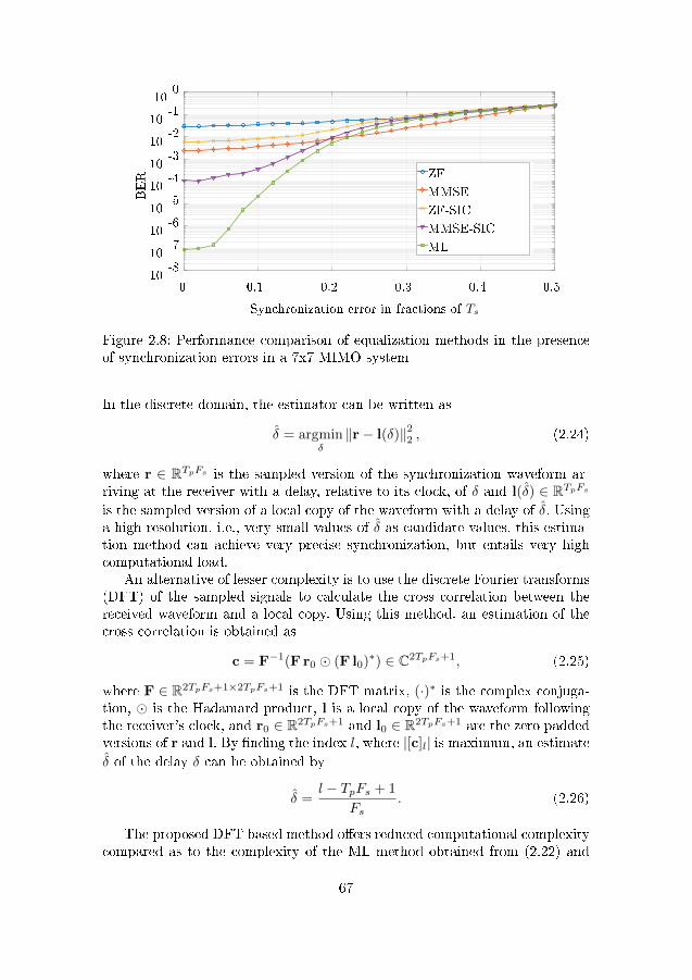
Synchronization error in fractions of Ts

0 0.1 0.2 0.3 0.4 0.5

BER

10-8

10-7

10-6

10-5

10-4

10-3

10-2

10-1

100

ZF

MMSE

ZF-SIC

MMSE-SIC

ML

Figure 2.8: Performance comparison of equalization methods in the presenceof synchronization errors in a 7x7 MIMO system

In the discrete domain, the estimator can be written as

δ = argminδ‖r− l(δ)‖22 , (2.24)

where r ∈ RTpFs is the sampled version of the synchronization waveform ar-riving at the receiver with a delay, relative to its clock, of δ and l(δ) ∈ RTpFsis the sampled version of a local copy of the waveform with a delay of δ. Usinga high resolution, i.e., very small values of δ as candidate values, this estima-tion method can achieve very precise synchronization, but entails very highcomputational load.

An alternative of lesser complexity is to use the discrete Fourier transforms(DFT) of the sampled signals to calculate the cross correlation between thereceived waveform and a local copy. Using this method, an estimation of thecross correlation is obtained as

c = F−1(F r0 � (F l0)∗) ∈ C2TpFs+1, (2.25)

where F ∈ R2TpFs+1×2TpFs+1 is the DFT matrix, (·)∗ is the complex conjuga-tion, � is the Hadamard product, l is a local copy of the waveform followingthe receiver's clock, and r0 ∈ R2TpFs+1 and l0 ∈ R2TpFs+1 are the zero paddedversions of r and l. By �nding the index l, where |[c]l| is maximum, an estimateδ of the delay δ can be obtained by

δ =l − TpFs + 1

Fs. (2.26)

The proposed DFT based method o�ers reduced computational complexitycompared as to the complexity of the ML method obtained from (2.22) and

67

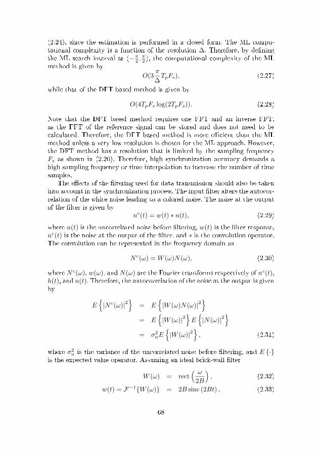
(2.24), since the estimation is performed in a closed form. The ML compu-tational complexity is a function of the resolution ∆. Therefore, by de�ningthe ML search interval as (−π2 ,π2 ), the computational complexity of the MLmethod is given by

O(3π

∆TpFs), (2.27)

while that of the DFT based method is given by

O(4TpFs log(2TpFs)). (2.28)

Note that the DFT based method requires one FFT and an inverse FFT,as the FFT of the reference signal can be stored and does not need to becalculated. Therefore, the DFT based method is more e�cient than the MLmethod unless a very low resolution is chosen for the ML approach. However,the DFT method has a resolution that is limited by the sampling frequencyFs as shown in (2.26). Therefore, high synchronization accuracy demands ahigh sampling frequency or time interpolation to increase the number of timesamples.

The e�ects of the �ltering used for data transmission should also be takeninto account in the synchronization process. The input �lter alters the autocor-relation of the white noise leading to a colored noise. The noise at the outputof the �lter is given by

nc(t) = w(t) ∗ n(t), (2.29)

where n(t) is the uncorrelated noise before �ltering, w(t) is the �lter response,nc(t) is the noise at the output of the �lter, and ∗ is the convolution operator.The convolution can be represented in the frequency domain as

N c(ω) = W (ω)N(ω), (2.30)

where N c(ω), w(ω), and N(ω) are the Fourier transforms respectively of nc(t),h(t), and n(t). Therefore, the autocorrelation of the noise at the output is givenby

E{|N c(ω)|2

}= E

{|W (ω)N(ω)|2

}= E

{|W (ω)|2

}E{|N(ω)|2

}= σ2

nE{|W (ω)|2

}, (2.31)

where σ2n is the variance of the uncorrelated noise before �ltering, and E {·}

is the expected value operator. Assuming an ideal brick-wall �lter

W (ω) = rect( ω

2B

), (2.32)

w(t) = F−1{W (ω)} = 2B sinc (2Bt) , (2.33)

68

where B is the bandwidth of the input �lter. Therefore, the noise samplesat the output of the �lter are uncorrelated only if they are sampled with 2Bsampling rate. A possible solution to this would be to increase the bandwidthof the �lter, which would, however, lead to a decrease in the e�ective SNR.Another problem of employing a very high sampling frequency is that it leadsto increased energetic demands at the receiver, and, therefore, defeats thepurpose of C-MIMO by leading to a decrease in energy e�ciency.

Figure 2.9 highlights the e�ects of noise correlation arising from oversam-pling during synchronization when using a 20 MHz tonal wave for the MLmethod. For the simulations, the sampling lasts for 2 periods of the tonalwave. The front end �lter is an ideal low pass brick wall �lter with bandwidthB = 22 MHz. The sampling frequency for simulations varies between two andten times the bandwidth of the front end �lter. The results show that, due tothe e�ects of noise correlation, the higher number of samples, obtained fromoversampling, results in a very small increase in performance.

SNR in dB

-10 -5 0 5 10

RMSE[s]

×10 -6

0

1

2

Fs = 2B

Fs = 2.5B

Fs = 3B

Fs = 5B

Fs = 7B

Fs = 10B

Figure 2.9: Performance of ML synchronization,f =20 MHz, B = 22 MHz

Figure 2.10 presents the synchronization performance, obtained by usingthe proposed DFT based method. In the proposed method, the performance isdegraded by noise only in very low SNR regimes, while in high SNR regimes,the major source of error comes from limited resolution. In this case, increasingthe sampling rate led to signi�cant performance improvement, despite intro-ducing noise correlation. Noise being not the dominant source of error, increas-ing the sampling rate results in higher resolution, and, therefore, in reducingthe errors caused by low discrete resolution. An alternative, when using a lowsampling frequency, is to interpolate the received samples of the waveform intime, thus leading to a higher sample rate. However, interpolation is bene�cialonly for low sampling frequencies, where the noise between samples is approx-

69

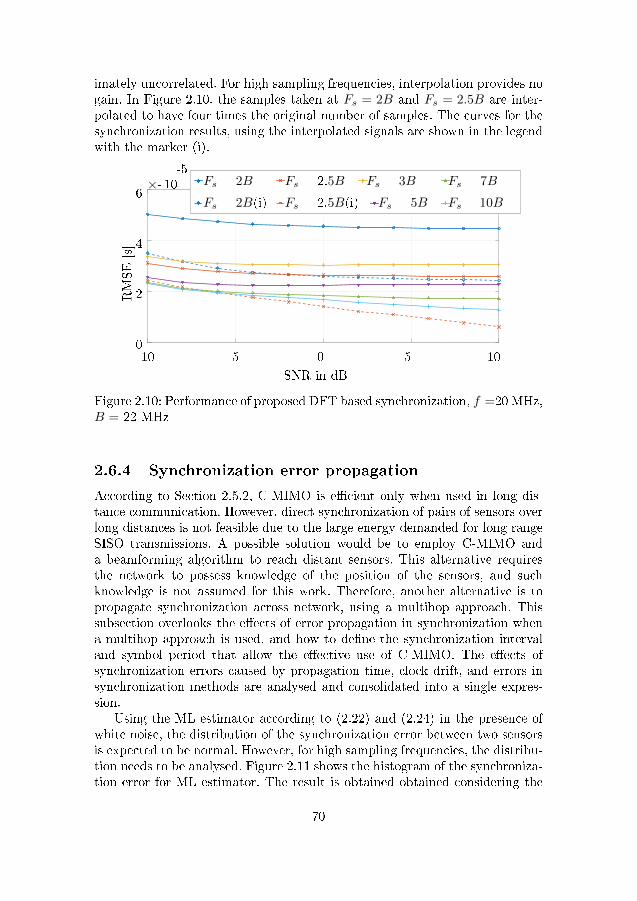
imately uncorrelated. For high sampling frequencies, interpolation provides nogain. In Figure 2.10, the samples taken at Fs = 2B and Fs = 2.5B are inter-polated to have four times the original number of samples. The curves for thesynchronization results, using the interpolated signals are shown in the legendwith the marker (i).

SNR in dB

-10 -5 0 5 10

RMSE[s]

×- 10-5

0

2

4

6Fs = 2B

Fs = 2B(i)

Fs = 2.5B

Fs = 2.5B(i)

Fs = 3B

Fs = 5B

Fs = 7B

Fs = 10B

Figure 2.10: Performance of proposed DFT based synchronization, f =20 MHz,B = 22 MHz

2.6.4 Synchronization error propagation

According to Section 2.5.2, C-MIMO is e�cient only when used in long dis-tance communication. However, direct synchronization of pairs of sensors overlong distances is not feasible due to the large energy demanded for long rangeSISO transmissions. A possible solution would be to employ C-MIMO anda beamforming algorithm to reach distant sensors. This alternative requiresthe network to possess knowledge of the position of the sensors, and suchknowledge is not assumed for this work. Therefore, another alternative is topropagate synchronization across network, using a multihop approach. Thissubsection overlooks the e�ects of error propagation in synchronization whena multihop approach is used, and how to de�ne the synchronization intervaland symbol period that allow the e�ective use of C-MIMO. The e�ects ofsynchronization errors caused by propagation time, clock drift, and errors insynchronization methods are analysed and consolidated into a single expres-sion.

Using the ML estimator according to (2.22) and (2.24) in the presence ofwhite noise, the distribution of the synchronization error between two sensorsis expected to be normal. However, for high sampling frequencies, the distribu-tion needs to be analysed. Figure 2.11 shows the histogram of the synchroniza-tion error for ML estimator. The result is obtained obtained considering the

70

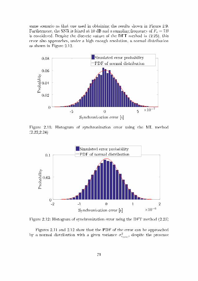
same scenario as that one used in obtaining the results shown in Figure 2.9.Furthermore, the SNR is feixed at 10 dB and a sampling frequency of Fs = 7Bis considered. Despite the discrete nature of the DFT method in (2.25), thiserror also approaches, under a high enough resolution, a normal distributionas shown in Figure 2.12.

Synchronization error [s]

×10−7-5 0 5

Probablity

0

0.02

0.04

0.06

0.08 Simulated error probability

PDF of normal distribution

Figure 2.11: Histogram of synchronization error using the ML method(2.22,2.24)

Synchronization error [s] ×10−6

-2 -1 0 1 2

Probability

0

0.05

0.1

Simulated error probability

PDF of normal distribution

Figure 2.12: Histogram of synchronization error using the DFT method (2.25)

Figures 2.11 and 2.12 show that the PDF of the error can be approachedby a normal distribution with a given variance σ2

εsync, despite the presence

71

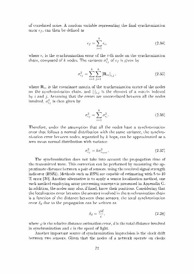
of correlated noise. A random variable representing the �nal synchronizationerror εf , can then be de�ned as

εf =

k∑i=1

εi, (2.34)

where εi is the synchronization error of the i-th node on the synchronizationchain, composed of k nodes. The variance σ2

εfof εf is given by

σ2εf

=

k∑i=1

k∑j=1

[Rεε]i,j , (2.35)

where Rεε is the covariance matrix of the synchronization errors of the nodeson the synchronization chain, and [·]i,j is the element of a matrix indexedby i and j. Assuming that the errors are uncorrelated between all the nodesinvolved, σ2

εfis then given by

σ2εf

=

k∑i=1

σ2εi . (2.36)

Therefore, under the assumption that all the nodes have a synchronizationerror that follows a normal distribution with the same variance, the synchro-nization error between nodes, separated by k hops, can be approximated as azero mean normal distribution with variance

σ2εf

= kσ2εsync

. (2.37)

The synchronization does not take into account the propagation time ofthe transmitted wave. This correction can be performed by measuring the ap-proximate distance between a pair of sensors, using the received signal strengthindicator (RSSI). Methods such as RSSI are capable of estimating with 5 to 10% error [30]. Another alternative is to apply a sensor localization method, onesuch method employing array processing concepts is presented in Appendix G.In addition, the nodes may also, if �xed, know their positions. Considering thatthe localization error between the sensors involved in the synchronization chainis a function of the distance between these sensors, the total synchronizationerror δd due to the propagation can be written as

δd =ϕd

c, (2.38)

where ϕ is the relative distance estimation error, d is the total distance involvedin synchronization and c is the speed of light.

Another important source of synchronization imprecision is the clock driftbetween two sensors. Given that the nodes of a network operate on clocks

72

with a given maximum drift rate ρ, they can drift apart at a maximum rateof 2ρ. A function ζ, de�ning the synchronization error between two sensors,which are k synchronization hops apart at time instant τ1 and which have lastsynchronized at time instant τ0, is given by

ς = N (0, kσ2εsync

) + δd + 2ρ∆τ , (2.39)

where ∆τ = τ1−τ0. As shown in Figures 2.6, 2.7, and 2.8, the synchronizationerror needs to be, at the most, 20 % of the symbol period to guarantee a goodBER performance. Therefore, to use the bene�ts of C-MIMO, the followingrelationship must hold

|N (0, kσ2εsync

)|+ δd + 2ρ∆τ ≤ 0.2Ts

|N (0, kσ2εsync

)| ≤ 0.2Ts − δd − 2ρ∆τ , (2.40)

where Ts is the symbol duration and

0.2Ts > δd + 2ρ(τ1 − τ0). (2.41)

The probability of the synchronization error being within the acceptable boundis then given by

erf

(0.2Ts − (δd + 2ρ∆τ )√

2kσεsync

). (2.42)

Therefore, when designing a WSN for operation with C-MIMO, the pa-rameters Ts and ∆τ need to be de�ned to ensure that the probability of thesynchronization error is within the acceptable bound. Also, care must be takento ensure that the energetic e�ciency of C-MIMO is not o�set by a large en-ergy demand from constant synchronization with a small ∆τ and with verylarge symbol periods Ts.

2.7 Adaptive C-MIMO Clustering

After achieving synchronization, C-MIMO can be used to improve energy e�-ciency of WSNs. However, prior to transmitting the data, a selection must bemade between using multi-hop or C-MIMO, since C-MIMO becomes bene�cialonly for long distance transmission, as explained in Section 2.4. Also, as WSNshave to be deployed even in harsh environments, the network must be capableof dealing with node outages (temporary or permanent), due to extreme heator cold conditions, temporary link outages due to eventual interference in agiven area or even energy depletion and consequent permanent failure of nodes.Routing algorithms developed for WSNs must be capable of choosing alterna-tive routes, if a given route becomes unavailable. Depending on the frequencyof such failures, di�erent routing algorithms can be employed. For networkswith fairly stable links, a routing table can be maintained at each node, with

73

either the full path to a given destination or only the next hop, depending onthe memory available with the nodes or the limitations in maximum packetoverhead. If the communication links are not reliable, up-to-date maintenanceof a large routing table in every node of the network might not be possible.In such cases, routing algorithms such as Ad hoc On-Demand Distance Vector(AODV), are generally used, in which paths are discovered only on demand,thus avoiding the need for maintaining routing tables on the nodes.

This Section is divided into two subsections. Subsection 2.7.1 details theproposed method for adaptively forming C-MIMO clusters according to the en-ergy e�ciency of di�erent cluster sizes and according to the impact of di�erentclusters sizes on the distribution of available energy over neighboring nodes.Subsection 2.7.2 presents the numerical simulations for the proposed method,highlighting positive e�ects on network lifetime and energy distribution.

2.7.1 Adaptive C-MIMO clustering

Possible C-MIMO formations for a given node can be represented as new edgeswith di�erent values on a graph. Therefore, the existence of C-MIMO can betransparent to the chosen routing algorithm. Moreover, since C-MIMO can beused with di�erent cluster sizes, it is important to choose the best possiblecluster size for reaching a given node in the network and representing it onthe routing graph as a vertex with the lowest possible cost. Another importantcharacteristic of C-MIMO is its ability to distribute energy consumption amongvarious nodes, and, depending on the number of neighbors of a given node, thenode may choose the neighbors that cooperate on a C-MIMO transmission tomaximize the life time of the network. .

Choosing between C-MIMO, multi-hop, and single-hop is not enough. SinceC-MIMO can be used with di�erent cluster sizes, it is important to choose thebest possible cluster size for reaching a given node in the network, representingit on the routing graph as a vertex with the lowest possible cost. However, min-imizing energy consumption is, by itself, not enough to maximize the lifetimeof a WSN. If energy consumption is low but the energy distribution is uneven,some nodes will fail before others. This distribution can be area dependent,for instance, regions with a high tra�c of information will tend to be depletedahead of the rest of the network. Node failures in such areas might lead to adisconnected network, reducing the e�ective lifetime of the network. Gener-ally, it is desirable that the nodes in a WSN have their energy reserves evenlydepleted, so that the network can stay fully connected as long as it is oper-ational. Therefore, by being aware of the energy reserves of its neighbours, anode can, when using C-MIMO, choose the con�guration and neighbours thatminimize the di�erence between the energy reserves of its neighbours.

This work proposes calculating the cost of a transmission as a function oftransmission power, cluster size and e�ects on the energy reserves of neigh-bours. The metric shown in (2.43) is used to de�ne the cost of a transmis-sion between a pair of nodes indexed by n = 1, . . . , L and m = 1, . . . , L. In

74

J(n,m

,w)

=

α(σ

0(n,w

)−σ

1(n,w

))+E

C−

MIM

O(w

),ifn6=m

andw6=

1andm∈Nn,w

Eintra

+Erx,

ifn6=m

andw

=1andm∈Nn,1

0,ifn

=m

∞,

ifn6=m

andm/∈Nn,w

(2.43)

75

this expression L is the number of nodes that compose the network, w =1, . . . ,W indexes the possible sizes for the C-MIMO clusters up to the limitW , EC−MIMO(w) is the energy cost for a C-MIMO transmission using clusterscomposed of w elements, σ0(n,m,w) and σ1(n,m,w) are the standard devi-ations of the energy available in the node's neighbours before and after thepossible C-MIMO transmission. Nn,w is the set of nodes that can be reachedby node n with a C-MIMO cluster size w. For a �xed cluster size, the nodesn and m always choose the neighbours with the highest amount of energy tomaximize the network lifetime. However, it is possible that some formations,even if the total energy cost is lower, cause the variance of the energy availableon the neighbours to increase too much. This means that the distribution ofthe available energy between the nodes is less uniform leading to some nodesrunning out of energy before others, and resulting in a disconnected network.Finally, α is a weighting factor that dictates the importance of keeping auniform energy reserve versus the importance of minimizing overall communi-cation energy consumption. If the transmit node n has knowledge about thestate of the energy reserves of the receive cluster it may also take into accountits changes on the calculation of the cost.

Each node n stores the cost relative to reaching a given neighbor in a costmatrix

[Rn]m,w = J(n,m,w) ∈ R. (2.44)

A graph used for routing can be set up by grouping all of the cost matricesfrom the nodes that form the network into a tensor structure

R = [R1|R2| . . . |RL] ∈ RL×L×W , (2.45)

where | denotes a stacking operation onto the �rst dimension. However, con-structing a graph based on this structure will result in vertices that are con-nected by multiple edges, since nodes can communicate using di�erent C-MIMO cluster sizes. To avoid this problem, some edges must be �ltered fromthe graph. This decision is simple, and can be based solely on the cost ofthe edges, leaving only the edges with the smallest cost between two vertices.Therefore, the decision on what cluster size sn,m to use to communicate be-tween a pair of nodes is given by

sn,m = argminw

[R]n,m,w ∈ N+. (2.46)

Algorithm 1 presents the proposed solution for choosing the optimal clusterformation for reaching a given node. A list of neighbors is present at eachnode and associated to it. Moreover, the list includes information about thenumber of nodes involved in the C-MIMO clusters for reaching the intendeddestination.

The cost can be a function of variables such as transmission power, clus-ter size and e�ects on the energy reserves of neighbours. This work uses thefollowing metric to de�ne the cost of C-MIMO transmission

J(σ20 , σ

21 , EC−MIMO) = α(σ2

0 − σ21) + EC−MIMO, (2.47)

76

Algorithm 1 Lower Cost Hop

1: load neighborList2: if routePacketReceived then3: nodes← routePacket.getOriginNodes()4: size← routePacket.clusterSize()5: cost← calculateCost(routePacket)6: for node : nodes do7: if neighborList.contains(node) then8: if node.cost() > cost then9: neighborList.remove(node)

10: neighborList.add(node, cost, size)11: end if12: else13: neighborList.add(node, cost, size)14: end if15: end for16: end if

where Ec-mimo is the energy cost for a C-MIMO transmission as computed in(2.18), σ2

o and σ21 are the variances of the energy available in the neighbour-

ing nodes, before and after the possible C-MIMO transmission. For a �xedcluster size, the node always chooses the neighbours with the highest amountof energy to maximize the network lifetime. However, it is possible that someformations, even if the total energy cost is low, signi�cantly increase the dif-ference between the energy levels of the neighbours. Thus, the distribution ofthe available energy between the nodes becomes less uniform. This will lead tosome nodes running out of energy before others do, which may ultimately re-sult in a disconnected network. Finally, α is the weighting factor that dictatesneed for maintaining a uniform energy reserve versus the need for minimizingoverall communication energy consumption. If the transmit node has knowl-edge about the state of the energy reserves of the receive cluster it may alsotake into account its changes on the calculation of the cost.

Other parameters such as delay, packet loss or available bandwidth mayalso be included in the metrics of cost function. If one of the nodes transmittingthe packet is not entered in the list, this entry is added on the neighbour's list.If an entry exists, the cost of the received packet is compared to the cost givenin the list (Lines 7 - 8 of Algorithm 1); if the cost of the received packet is lowerthan the cost given in the list, this entry is replaced (Lines 9 � 10 of Algorithm1). This optimal entry can be then sent to the transmitting node or cluster,assuming that all connection characteristics are re�ective, or the transmittingnode or cluster itself may use the response to calculate the cost associated withthe reverse path. Using this algorithm, a node can decide when a packet needsto be forwarded, and the optimal number of nodes that need to be involved ina C-MIMO transmission to reach a certain neighbour on the list. The graph

77

structure is not modi�ed; therefore, classic graph routing algorithms can stillbe employed.

The proposed algorithm can take advantage of the C-MIMO techniqueand of the traditional multi-hop technique to achieve the lowest possible en-ergy consumption in the network. The same algorithm is also used to selectthe optimal number of cluster members that must be present in a C-MIMOtransmission. Thus, C-MIMO transmissions can be adaptively employed bymodifying the cluster con�gurations to suit the changes in the network topol-ogy, but without disturbing the operation of standard transmission techniques.

2.7.2 Numerical Simulations

For numerical simulations, this work assumes that the sensors follow the com-munication characteristics of Harvard Mica2 platform [99]. An area of 100 m ×100 m is �lled with 300 nodes placed with coordinates following independentuniform distribution. These nodes are capable of transmitting with a powerranging from −20 dBm to 10dBm, with respective current drains at the ra-dio ranging from 3.7 mA to 21.5 mA. The current drain at the radios duringreception is 7 mA, which is considerably higher than the drain on low powertransmissions.

The noise power density at the radios during reception is considered to be−174 dBm/Hz and the radios are assumed to have a 5 dB noise �gure. Thecommunication is assumed to take e�ect by using 2.4 GHz center frequencyand a 20 MHz channel, treated with a 22 MHz �lter. The resulting noise powerat the receiver was −96dBm.

Transmissions follow the free-space path loss model, and the antennas haveno gain. Therefore, the attenuation in dB of a signal, received d kilometres awayfrom its receiver, is given by

Loss(d) = 20 log(d) + 100.05. (2.48)

Following the results shown in Figure 2.18, the desired system BER is set to10−2. The SNR necessary to achieve the same SNR varies with the size of theC-MIMO cluster; larger cluster formation requires lower SNR to reach a givenBER.

According to [5], the probability that a given node has at least n neighbourslocated at most r distance units away is given by

P (n) = 1−n−1∑i=0

(ρπr2)i

i!e−ρπr

2

, (2.49)

where ρ is the node density of the network. For the simulations r = 7.9 m,which is the maximum distance reachable with an SNR of 10 dB using atransmission power of -8 dBm. This shows that the probabilities of a nodehaving at least 2, 3 or 4 neighbours are 98 %, 93.2 %, and 83.8 % respectively.

78

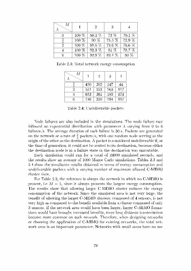
λM

1 2 3 4

0 100 % 88.3 % 73 % 70.1 %23 100 % 90 % 75.5 % 72.9 %2 100 % 91.8 % 78.6 % 76.6 %4 100 % 92.3 % 81 % 78.7 %6 100 % 92.9 % 82.4 % 80 %

Table 2.3: Total network energy consumption

λM

1 2 3 4

23 450 202 147 442 551 252 163 1174 652 261 183 1746 746 320 194 187

Table 2.4: Undeliverable packets

Node failures are also included in the simulations. The node failure ratefollowed an exponential distribution with parameter λ varying from 0 to 6failures/s. The average duration of each failure is 30 s. Packets are generatedon the network at a rate of 2

3 packets/s, with one random node serving as theorigin of the other as the destination. A packet is considered undeliverable if, atthe time of generation, it could not be routed to its destination, because eitherthe destination node is in a failure state or the destination was unroutable.

Each simulation could run for a total of 24000 simulated seconds, andthe results show an average of 1000 Monte Carlo simulations. Tables 2.3 and2.4 show the simulation results obtained in terms of energy consumption andundeliverable packets with a varying number of maximum allowed C-MIMOcluster sizes.

For Table 2.3, the reference is always the network in which no C-MIMO ispresent, i.e M = 1, since it always presents the largest energy consumption.The results show that allowing larger C-MIMO cluster reduces the energyconsumption of the network. Since the simulated area is not very large, thebene�t of allowing the larger C-MIMO clusters, composed of 4 sensors, is notvery high as compared to the bene�t available from a cluster composed of only3 sensors. If the network area would have been larger, larger C-MIMO forma-tions would have brought increased bene�ts, since long distance transmissionsbecome more common on such network. Therefore, when designing networksor choosing the application of C-MIMO for existing networks, the total net-work area is an important parameter. Networks with small areas have no use

79

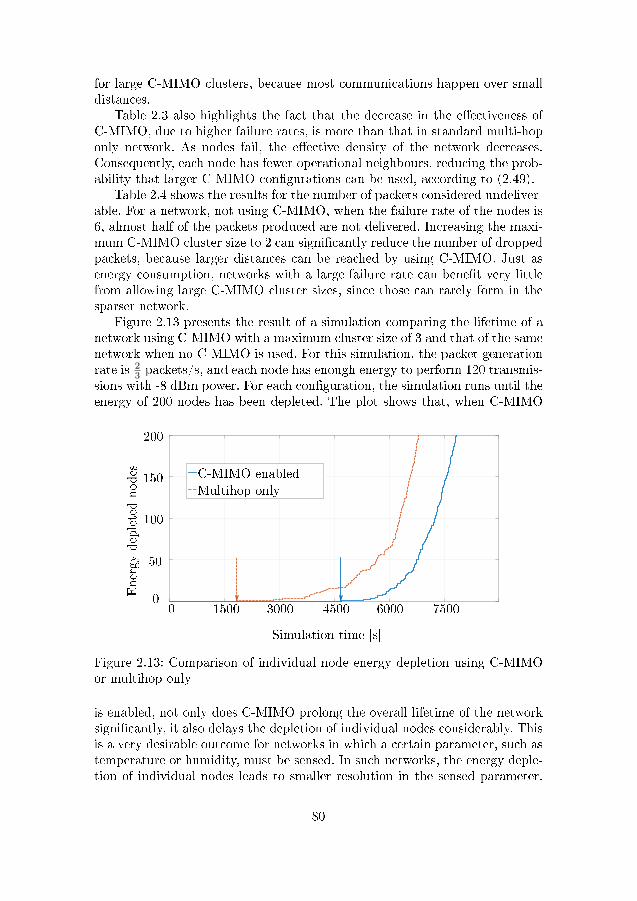
for large C-MIMO clusters, because most communications happen over smalldistances.

Table 2.3 also highlights the fact that the decrease in the e�ectiveness ofC-MIMO, due to higher failure rates, is more than that in standard multi-hoponly network. As nodes fail, the e�ective density of the network decreases.Consequently, each node has fewer operational neighbours, reducing the prob-ability that larger C-MIMO con�gurations can be used, according to (2.49).

Table 2.4 shows the results for the number of packets considered undeliver-able. For a network, not using C-MIMO, when the failure rate of the nodes is6, almost half of the packets produced are not delivered. Increasing the maxi-mum C-MIMO cluster size to 2 can signi�cantly reduce the number of droppedpackets, because larger distances can be reached by using C-MIMO. Just asenergy consumption, networks with a large failure rate can bene�t very littlefrom allowing large C-MIMO cluster sizes, since those can rarely form in thesparser network.

Figure 2.13 presents the result of a simulation comparing the lifetime of anetwork using C-MIMO with a maximum cluster size of 3 and that of the samenetwork when no C-MIMO is used. For this simulation, the packet generationrate is 2

3 packets/s, and each node has enough energy to perform 120 transmis-sions with -8 dBm power. For each con�guration, the simulation runs until theenergy of 200 nodes has been depleted. The plot shows that, when C-MIMO

Simulation time [s]

Energydepletednodes

0

200

150

100

50

C-MIMO enabled

Multihop only

01500 3000 4500 6000 7500

Figure 2.13: Comparison of individual node energy depletion using C-MIMOor multihop only

is enabled, not only does C-MIMO prolong the overall lifetime of the networksigni�cantly, it also delays the depletion of individual nodes considerably. Thisis a very desirable outcome for networks in which a certain parameter, such astemperature or humidity, must be sensed. In such networks, the energy deple-tion of individual nodes leads to smaller resolution in the sensed parameter.

80

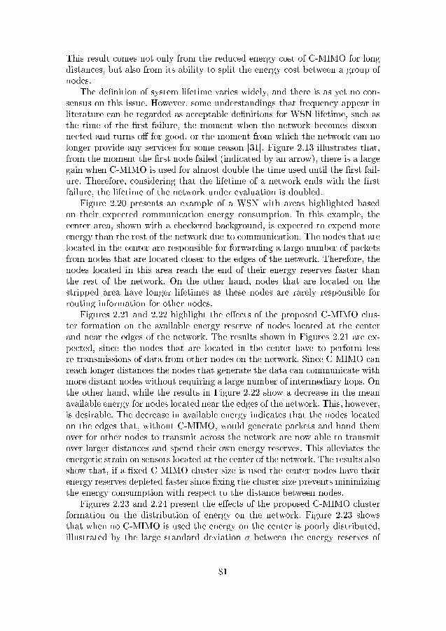
This result comes not only from the reduced energy cost of C-MIMO for longdistances, but also from its ability to split the energy cost between a group ofnodes.

The de�nition of system lifetime varies widely, and there is as yet no con-sensus on this issue. However, some understandings that frequency appear inliterature can be regarded as acceptable de�nitions for WSN lifetime, such asthe time of the �rst failure, the moment when the network becomes discon-nected and turns o� for good, or the moment from which the network can nolonger provide any services for some reason [31]. Figure 2.13 illustrates that,from the moment the �rst node failed (indicated by an arrow), there is a largegain when C-MIMO is used for almost double the time used until the �rst fail-ure. Therefore, considering that the lifetime of a network ends with the �rstfailure, the lifetime of the network under evaluation is doubled.

Figure 2.20 presents an example of a WSN with areas highlighted basedon their expected communication energy consumption. In this example, thecenter area, shown with a checkered background, is expected to expend moreenergy than the rest of the network due to communication. The nodes that arelocated in the center are responsible for forwarding a large number of packetsfrom nodes that are located closer to the edges of the network. Therefore, thenodes located in this area reach the end of their energy reserves faster thanthe rest of the network. On the other hand, nodes that are located on thestripped area have longer lifetimes as these nodes are rarely responsible forrouting information for other nodes.

Figures 2.21 and 2.22 highlight the e�ects of the proposed C-MIMO clus-ter formation on the available energy reserve of nodes located at the centerand near the edges of the network. The results shown in Figures 2.21 are ex-pected, since the nodes that are located in the center have to perform lessre-transmissions of data from other nodes on the network. Since C-MIMO canreach longer distances the nodes that generate the data can communicate withmore distant nodes without requiring a large number of intermediary hops. Onthe other hand, while the results in Figure 2.22 show a decrease in the meanavailable energy for nodes located near the edges of the network. This, however,is desirable. The decrease in available energy indicates that the nodes locatedon the edges that, without C-MIMO, would generate packets and hand themover for other nodes to transmit across the network are now able to transmitover larger distances and spend their own energy reserves. This alleviates theenergetic strain on sensors located at the center of the network. The results alsoshow that, if a �xed C-MIMO cluster size is used the center nodes have theirenergy reserves depleted faster since �xing the cluster size prevents minimizingthe energy consumption with respect to the distance between nodes.

Figures 2.23 and 2.24 present the e�ects of the proposed C-MIMO clusterformation on the distribution of energy on the network. Figure 2.23 showsthat when no C-MIMO is used the energy on the center is poorly distributed,illustrated by the large standard deviation σ between the energy reserves of

81

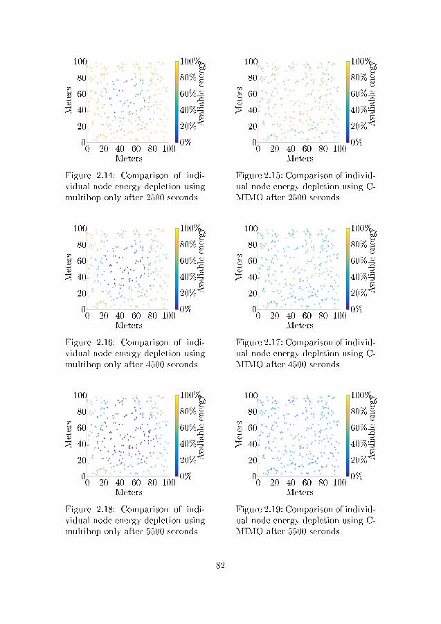
Meters0 20 40 60 80 100

Meters

0

20

40

60

80

100

Avaliableenergy

0%

20%

40%

60%

80%

100%

Figure 2.14: Comparison of indi-vidual node energy depletion usingmultihop only after 2500 seconds

Meters0 20 40 60 80 100

Meters

0

20

40

60

80

100

Avaliableenergy

0%

20%

40%

60%

80%

100%

Figure 2.15: Comparison of individ-ual node energy depletion using C-MIMO after 2500 seconds

Meters0 20 40 60 80 100

Meters

0

20

40

60

80

100

Avaliableenergy

0%

20%

40%

60%

80%

100%

Figure 2.16: Comparison of indi-vidual node energy depletion usingmultihop only after 4500 seconds

Meters0 20 40 60 80 100

Meters

0

20

40

60

80

100

Avaliableenergy

0%

20%

40%

60%

80%

100%

Figure 2.17: Comparison of individ-ual node energy depletion using C-MIMO after 4500 seconds

Meters0 20 40 60 80 100

Meters

0

20

40

60

80

100

Avaliableenergy

0%

20%

40%

60%

80%

100%

Figure 2.18: Comparison of indi-vidual node energy depletion usingmultihop only after 5500 seconds

Meters0 20 40 60 80 100

Meters

0

20

40

60

80

100

Avaliableenergy

0%

20%

40%

60%

80%

100%

Figure 2.19: Comparison of individ-ual node energy depletion using C-MIMO after 5500 seconds

82

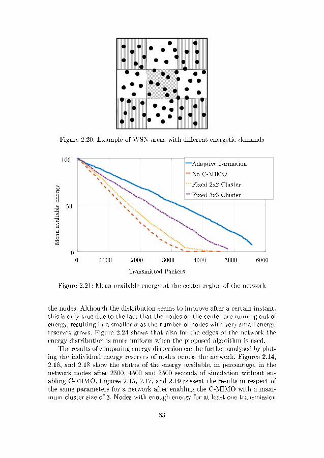
Figure 2.20: Example of WSN areas with di�erent energetic demands

Transmitted Packets

0 1000 2000 3000 4000 5000 6000

Meanavaliableenergy

0

50

100Adaptive Formation

No C-MIMO

Fixed 2x2 Cluster

Fixed 3x3 Cluster

Figure 2.21: Mean available energy at the center region of the network

the nodes. Although the distribution seems to improve after a certain instant,this is only true due to the fact that the nodes on the center are running out ofenergy, resulting in a smaller σ as the number of nodes with very small energyreserves grows. Figure 2.24 shows that also for the edges of the network theenergy distribution is more uniform when the proposed algorithm is used.

The results of comparing energy dispersion can be further analysed by plot-ing the individual energy reserves of nodes across the network. Figures 2.14,2.16, and 2.18 show the status of the energy available, in percentage, in thenetwork nodes after 2500, 4500 and 5500 seconds of simulation without en-abling C-MIMO. Figures 2.15, 2.17, and 2.19 present the results in respect ofthe same parameters for a network after enabling the C-MIMO with a maxi-mum cluster size of 3. Nodes with enough energy for at least one transmission

83

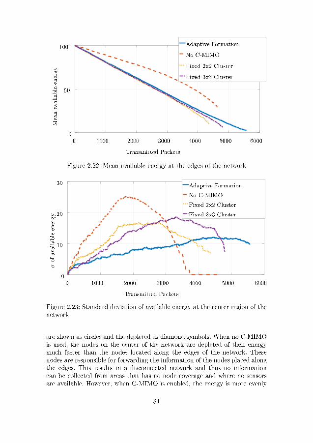
Transmitted Packets

0 1000 2000 3000 4000 5000 6000

Meanavaliableenergy

0

50

100 Adaptive Formation

No C-MIMO

Fixed 2x2 Cluster

Fixed 3x3 Cluster

Figure 2.22: Mean available energy at the edges of the network

Transmitted Packets

0 1000 2000 3000 4000 5000 6000

σofavaliableenergy

0

10

20

30 Adaptive Formation

No C-MIMO

Fixed 2x2 Cluster

Fixed 3x3 Cluster

Figure 2.23: Standard deviation of available energy at the center region of thenetwork

are shown as circles and the depleted as diamond symbols. When no C-MIMOis used, the nodes on the center of the network are depleted of their energymuch faster than the nodes located along the edges of the network. Thesenodes are responsible for forwarding the information of the nodes placed alongthe edges. This results in a disconnected network and thus no informationcan be collected from areas that has no node coverage and where no sensorsare available. However, when C-MIMO is enabled, the energy is more evenly

84

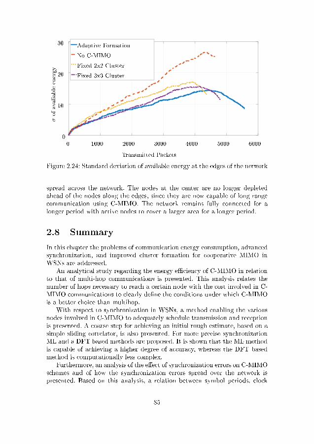
Transmitted Packets

0 1000 2000 3000 4000 5000 6000

σofavaliableenergy

0

10

20

30 Adaptive Formation

No C-MIMO

Fixed 2x2 Cluster

Fixed 3x3 Cluster

Figure 2.24: Standard deviation of available energy at the edges of the network

spread across the network. The nodes at the center are no longer depletedahead of the nodes along the edges, since they are now capable of long rangecommunication using C-MIMO. The network remains fully connected for alonger period with active nodes to cover a larger area for a longer period.

2.8 Summary

In this chapter the problems of communication energy consumption, advancedsynchronization, and improved cluster formation for cooperative MIMO inWSNs are addressed.

An analytical study regarding the energy e�ciency of C-MIMO in relationto that of multi-hop communications is presented. This analysis relates thenumber of hops necessary to reach a certain node with the cost involved in C-MIMO communications to clearly de�ne the conditions under which C-MIMOis a better choice than multihop.

With respect to synchronization in WSNs, a method enabling the variousnodes involved in C-MIMO to adequately schedule transmission and receptionis presented. A coarse step for achieving an initial rough estimate, based on asimple sliding correlator, is also presented. For more precise synchronizationML and a DFT based methods are proposed. It is shown that the ML methodis capable of achieving a higher degree of accuracy, whereas the DFT basedmethod is computationally less complex.

Furthermore, an analysis of the e�ect of synchronization errors on C-MIMOschemes and of how the synchronization errors spread over the network ispresented. Based on this analysis, a relation between symbol periods, clock

85

drift, and synchronization error is derived. This can be used to ensure that anacceptable degree of synchronization is achieved for a given data rate by usingC-MIMO.

Finally, a method that allows the formation of e�cient C-MIMO clusteris proposed, availing the bene�ts provided by this communication scheme,such as reduced energy cost and better distribution of energy demand. Theproposed method is shown to extend network lifetime by reducing individualnode failures and to achieve networks with a more homogeneous distributionof energy between the nodes, resulting in networks that remain fully connectedfor longer periods.

86

Chapter 3

Array ProcessingLocalization for VehicularNetworks

In this chapter the following research question is addressed:Can array processing techniques be used to reliably estimate position of vehiclesand pedestrians in vehicular scenarios based on their radio transmissions?

3.1 Overview and Contribution

The remainder of this section is organized as follows:

� Motivation: The concept of vehicular networks and smart transporta-tion systems is introduced. The problem of localizing vehicles and roadusers in such environment is shown and a solution from an array pro-cessing perspective is introduced.

� Data Model: The broadband spherical wave data model of a signalreceived at an antenna array is de�ned.

� Space-Alternating Generalized Expectation Maximization (SAGE)Algorithm:Here, the space-alternating generalized expectation-maximization(SAGE) algorithm for parameter estimation is brie�y explained.

� Scenario Description: The assumed scenario for the localization invehicular networks is shown and some constraints are discussed.

� Array Processing Localization: In this section three di�erent ap-proaches for localization in vehicular scenarios are presented. These ap-proaches vary in performance and complexity and can be applied basedon the speci�c performance and output rate requirements.

87

� Three Dimensional DOA Based Estimation: Here, the DOA basedmethod is extended to the three dimensional case considering the esti-mation of position and attitude of UAVs as an application.

� Simulation Results: Finally, the performance of the proposed methodsis shown by means of numerical simulations. A set of such simulationsis performed using a real measured response from an antenna array tovalidate the proposed methods using real data.

The research contributions presented in this chapter are:

1. A DOA only localization method capable of localizing transmitters nearto a vehicle at a low computational cost.

2. A localization method based on range and DOA estimations performedat independent subarrays. The geometrical relationship between the in-dividual estimates is used to speed up the rate of convergence of theSAGE algorithm on the individual subarrays.

3. A novel parametrization for the received waveform data model allowingjoint localization estimation to be performed at both subarrays simulta-neously.

4. Localization methods that do not require the transmission of speci�clocation data that can be used to mitigate spoo�ng attacks in VANETs.

3.2 Motivation

Vehicular ad hoc networks (VANETs) are a promising technology with ap-plications such as road safety, tra�c control, automated vehicle control, andplatooning [60]. Many of such applications require the localization of all vehi-cles that compose a VANET to be known or estimated with a high degree ofaccuracy. Furthermore, not only must the accuracy be su�cient the estimatemust also be reliable. Road safety, automated vehicles, and road control requirethe vehicles to be able to process and to estimate the position of vulnerableroad users (VRUs), as well as the position of the other vehicles in the vicinity,so that they can operate adequately.

For the detection of VRUs, a variety of methods have been proposed. Thesemethods must be precise and fast enough to meet di�erent safety requirementsregarding a multitude of possible situations. A set of requirements for VRUdetection systems is presented in [49]. Most of these methods for VRU detec-tion in the literature rely on computer vision [45]. These methods can providean accuracy of up to 75% [35,46], which might be insu�cient for safety-criticalsystems such as collision detection and prevention/avoidance.

The localization of other vehicles is also of interest and can be obtained byusing a variety of methods. One of the main source of location information in

88

a VANET is the usage of Global Navigation Satellite Systems (GNSS) infor-mation to obtain, for each vehicle, an estimate of it's location. GNSS such asthe Global Positioning System (GPS) can provide location information witha mean error of �fteen meters in urban environments [83]. However, this ac-curacy is not su�cient for emerging applications in Intelligent transportationsystems (ITS) such as platooning [102] or for safety-critical applications. Fur-thermore, GNSS requires that a set of at least four line of sight signals arereceived from di�erent satellites, this is not always possible in dense urbanenvironments, leading to a possible large number of outages.

Other means of vehicle positioning such as using the received signal strengthindicator (RSSI) of the received data signals [88] can also be used and are ca-pable of complementing GNSS information and making safety applicationspossible. Other vehicle positioning approaches such as dead reckoning [57] canbe used to provide position estimation during outages of GNSS. However,these approaches assume that the information that is provided by neighboringvehicles can be trusted.

Even in scenarios where the position provided by some vehicles can beassumed to be reliable and precise enough for the application at hand problemssuch as spoo�ng can still emerge. In a spoo�ng attack it is possible to falsifyGNSS information such that a vehicle will obtain a position estimation that hasbeen altered by the attacker. Furthermore, since GNSS information is usuallyspread using a data dissemination method [85], the position information can befalsi�ed by the transmitting vehicle or by intermediary vehicles of the network.Position veri�cation approaches [65] for VANETs can mitigate but not fullysolve the problem of spoo�ng attacks.

Approaches that leverage the presence of inertial sensors in smartphonesinside a vehicle, using them to provide robust positioning for vehicles in a net-work have been proposed [22], providing an accuracy of approximately 7 me-ters. Methods for localization in vehicular networks based on building a socialmodel of the interactions of vehicles in the networks can provide position esti-mates with an accuracy of up to 10 meters [67]. While these methods providean improvement over a GNSS only positioning solution, the accuracy providedis not su�cient for the safety-critical applications in vehicular networks. Ap-proaches that rely on a dedicated localization infrastructure can provide exactlocalization methods with an accuracy superior to one meter [94] at the costof an increased system complexity and may not be available outside of urbanand busy roads.

A promising technology that can be applied to VANETs is the Multiple-input multiple-output (MIMO) communication scheme. MIMO has been usedin modern wireless communications standards to allow for better spectral e�-ciency, faster data rates, and more robust communication. The usage of MIMOin vehicular network scenarios has been proposed to improve the network per-formance [103], suppress possible jamming attacks [58], and increase networkcapacity [55]. The antennas used for MIMO applications can be leveraged

89

to provide accurate positioning of vehicles on the network, without requiringa dedicated infrastructure. Since the usage of MIMO requires the presence ofmultiple antennas at both receiver and transmitter, this antennas can be setupas, for instance, linear antenna arrays to allow the application of array signalprocessing techniques to provide an extra source of localization information onthe network.

This work proposes the usage of array signal processing tools for direc-tion of arrival (DOA) estimation to passively estimate the position of vehiclestransmitting a signal. The proposed method allows the position of a vehicleto be estimated by all vehicles within its communication range passively. Thisestimation does not require the transmission of localization speci�c messages,thus, it can be used to alleviate the network load. The proposed estimationmethod is also robust to data falsi�cation since it relies on parameters thatare estimated on the physical layer and cannot be altered or falsi�ed easily,requiring a very complex system to do so.

3.3 Data Model

The assumed model considers a set of L wavefronts impinging onto an ULAcomposed ofM antenna elements. The signal is assumed to be transmitted us-ing an orthogonal frequency-division multiplexing (OFDM) scheme composedof K subcarriers. This model takes into account the curvature of the sphericalwavefront. Using the Fresnel approximation, after removing the cyclic pre�xand taking the discrete Fourier transform (DFT) of the received signal thespace-frequency response of the k-th subcarrier received at antenna m duringtime snapshot t can be written as

xm,k,t =

L∑l=1

sl,k,tαm,l,keωl(m−1)+ψl(m−1)2 · ej2πk∆f (τl)

+ nm,k,t, (3.1)

where,

ωl = −2π∆m sin(θl)

λ, (3.2)

ψl =π∆2

m cos2(θl)

λrl, (3.3)

sl,k,t is the symbol transmitted by the l-th source at time instant t, αm,l,k isthe complex channel gain coe�cient, ∆m is the separation between antennaelements of the array, θl is the DOA of the l-th signal, rl is the range of thel-th source, λ is the wavelength of the carrier frequency, ∆f is the frequencyseparation between the subcarriers of the OFDM signal, τl is the propagationdelay of the l-th received signal, and nm,k,t is additive complex white Gaussiannoise.

90

The model can be rewritten in matrix form as

X = D(A � Z)S + N ∈ CMK×T , (3.4)

where � is the Khatri-Rao product, T is the total number of snapshots avail-able, D is a diagonal matrix containing the channel gain coe�cients, S ∈ CL×Tcontains the symbols transmitted by the L sources for all T snapshots, N ∈CMK×T is the noise matrix with its entries drawn from CN (0, σ2

n), and

A = [a(θ1, r1),a(θ2, r2), ...,a(θL, rL)] ∈ CM×L, (3.5)

Z = [z(τ1), z(τ2), ..., z(τL)] ∈ CK×L, (3.6)

with

a(θl, rl) =[1, eωl+ψl , . . . , eωl(M−1)+ψl(M−1)2

]T∈ CM×1, (3.7)

z(τl) =[ej2π1∆f (τl), ej2π2∆f (τl), . . . , ej2πK∆f (τl)

]T,∈ CK×1, (3.8)

being the space and frequency steering vectors of the l-th received signal re-spectively.

3.4 Space-Alternating Generalized ExpectationMaximization (SAGE) Algorithm

The SAGE algorithm is a generalization of the EM algorithm, both are al-gorithms used to derive maximum likelihood estimates in an iterative fash-ion. The idea behind the these algorithms is to split an L-dimensional multi-dimensional problem that might be too computationally demanding to performwithin an expected time constrain into L separate one-dimensional problemsthat can be solved within a shorter time. SAGE and EM utilize the conceptof hidden data space to avoid dealing with the complete observed data set. Inthe case of a signal received at the array, the complete data can be written asa function of the hidden data space

Y = X1 + X2 + · · ·+ XL, (3.9)

Xl = h(pl)sl + nl, (3.10)

where h is a steering vector constructed from the parameter vector pl =[p1l , p

2l , . . . , p

Pl ], sl is the symbol vector and n is the noise component and is

complex normally distributed with zero mean and variance σ2l .

91

An iteration of SAGE is split into two di�erent steps, the expectation andthe maximization steps. The expectation step of the c-th cycle of the i-thiteration of SAGE is given by

Xl(p[i,c−1]l , s

[i,c−1]l ) = E[Xl|Y,p

[i,c−1]l , s

[i,c−1]l ]

= h(p[i,c−1]l )s

[i,c−1]l

+1

L(Y −

L∑j=1j 6=i

h(p[i,c−1]j )s

[i,c−1]j ) (3.11)

RXl= Xl(p

[i,c−1]l , s

[i,c−1]l )Xl(p

[i,c−1]l , s

[i,c−1]l )H (3.12)

The maximization step can then be performed, to estimate the parameter

pjl the remaining parameters of p[i,c−1]l are kept �xed and the following problem

is solved

pjl[i,c]

= argmaxpjl

h(p[i,c−1]l )HRXl

(p[i,c−1]l , s

[i,c−1]l )h(p

[i,c−1]l .) (3.13)

The transmitted symbols are estimated following

s[i,c]l = h(p

[i,c]l )HXl(p

[i,c−1]l , s

[i,c−1]l .) (3.14)

The SAGE algorithm iterates over the parameters of all received signalsuntil a convergence threshold is met. For the remainder of this work the su-perscripts for iteration and cycle will be omitted to simplify the notation.

3.5 Scenario Description

This work assumes that the vehicles connected to the VANET are equippedwith two linear antenna arrays at two distinct locations on their frames. Figure3.1 depicts an example of a vehicle with antenna arrays equipped at the wingmirror position triangulating the position of a VRU.

To avoid ambiguities in DOA estimation the antenna elements of the arraymust be placed no further than half a wave length apart. Assuming the com-munication occurs at the 5.8 GHz frequency band and that DOA estimationis to be done at carrier frequency the antenna elements can be placed as far as2.5 cm apart. Antenna elements can be installed close together to allow moreantennas to be installed on the same area or to reduce the total size of theantenna array, however this comes at the cost of increasing mutual couplingbetween antenna elements. This work assumes that the antenna arrays areinstalled at the wing mirror position of the vehicles composing the network.

92

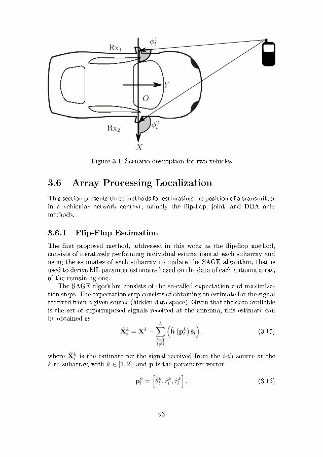
Rx1

Rx2

φ1l

φ2l

O

Y

X

Figure 3.1: Scenario description for two vehicles

3.6 Array Processing Localization

This section presents three methods for estimating the position of a transmitterin a vehicular network context, namely the �ip-�op, joint, and DOA onlymethods.

3.6.1 Flip-Flop Estimation

The �rst proposed method, addressed in this work as the �ip-�op method,consists of iteratively performing individual estimations at each subarray andusing the estimates of each subarray to update the SAGE algorithm, that isused to derive ML paramter estimates based on the data of each antenna array,of the remaining one.

The SAGE algorithm consists of the so-called expectation and maximiza-tion steps. The expectation step consists of obtaining an estimate for the signalreceived from a given source (hidden data space). Given that the data availableis the set of superimposed signals received at the antenna, this estimate canbe obtained as

Xki = Xk −

L∑l=1l 6=i

(h(pkl)sl

), (3.15)

where Xki is the estimate for the signal received from the i-th source at the

k-th subarray, with k ∈ [1, 2], and p is the parameter vector

pkl =[θkl , r

kl , τ

kl

], (3.16)

93

where θkl , τkl , and rkl are the azimuth, delay, and range estimates for the l-

th source at the k-th subarray, respectively. sl is a vector with the estimatesof the symbols transmitted by the l-th source. Furthermore, h is the currentestimate of h, which is de�ned as

h(pkl)

=[

a(θkl , r

kl

)⊗ z

(τkl) ]∈ CMK×1. (3.17)

Following the expectation step, the maximization step transforms a D-dimensional estimation problem into D one-dimensional estimation problemsby �xing all except one of the parameters during the estimation. Let the costfunction d be de�ned as

d(pkl ,X

k)

=∣∣∣h (pkl )H Xk

∣∣∣2 . (3.18)

To obtain a complete estimate of p the algorithm will solve the set of Doptimization problems. These optimization problems can be written as

θkl = argmaxθkl

d(pkl , X

kl

), (3.19)

rkl = argmaxrkl

d(pkl , X

kl

), (3.20)

τkl = argmaxτkl

d(pkl ,

ˆXkl

). (3.21)

To estimate each parameter, a di�erent set of parameters is �xed, and a one-dimensional search is performed over the parameter that is currently beingestimated. This process is iteratively performed until the estimates of all pa-rameters converges.

Once the range and DOA parameter has been estimated for one of thesubarrays, an estimate of the position of the transmitter can be obtained.Assuming that the center of a line crossing the car and both wing mirrors tobe the origin of the reference coordinate system, denoted as O, it is necessaryto obtain the angle φkl , which, as shown in Figure 3.1, is a complementaryangle to θkl . Thus, the relationship between φkl and θ

kl is given by

φkl = − 1

θkl + 2π. (3.22)

With this parameter at hand and following the coordinate system shown inFigure 3.1, an estimate of the position of the l-th transmitter with respect tothe signal received at the k-th subarray Rxk is given by

xkl = rkl cos(φkl ) + xRxk, (3.23)

ykl = rkl sin(φkl ). (3.24)

94

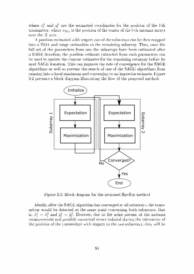
where xkl and ykl are the estimated coordinates for the position of the l-thtransmitter. where xRxl is the position of the center of the l-th antenna arraysover the X axis.

A position estimated with respect one of the subarrays can be then mappedinto a DOA and range estimation to the remaining subarray. Thus, once thefull set of the parameters from one the subarrays have been estimated aftera SAGE iteration, the position estimate extracted from such parameters canbe used to update the current estimates for the remaining subarray before itsnext SAGE iteration. This can improve the rate of convergence for the SAGEalgorithms as well as prevent the search of one of the SAGE algorithms fromrunning into a local maximum and converging to an imprecise estimate. Figure3.2 presents a block diagram illustrating the �ow of the proposed method.

Expectation

Maximization

Expectation

Maximization

Initialize

Converged?No

End

Yes

Subarr

ay 1

Subarra

y 2

Figure 3.2: Block diagram for the proposed �ip-�op method

Ideally, after the SAGE algorithm has converged at all subarrays, the trans-mitter would be detected at the same point concerning both subarrays, thatis, x1

l = x2l and y1

l = y2l . However, due to the noise present at the antenna

measurements and possible numerical errors induced during the estimation ofthe position of the transmitter with respect to the two subarrays, they will be

95

di�erent, thus x1l 6= x2

l and y1l 6= y2

l . To solve this, the �nal estimation can begiven as a function of the estimates for each of the subarrays as:

xl =γx1

l + νx2l

γ + ν, (3.25)

yl =γy1

l + νy2l

γ + ν, (3.26)

where γ and ν are weighting coe�cients that represent how reliable are theposition estimates of each subarray. These weights can be set, for instance, asa function of the received signal strength at each of the subarrays. In this caseγ and ν are given by

γ =

(a(θ1

l )⊗ z(τ1l

))H

X1 X1 H(a(θ1

l )⊗ z(τ1l

))(a(θ1

l )⊗ z (τ1l ))H (

a(θ1l )⊗ z (τ1

l ))tr(X1 X1 H

) , (3.27)

ν =

(a(θ2

l )⊗ z(τ2l

))H

X2 X2 H(a(θ2

l )⊗ z(τ2l

))(a(θ2

l )⊗ z (τ2l ))H (

a(θ2l )⊗ z (τ2

l ))tr(X2 X2 H

) . (3.28)

3.6.2 Joint Direct Position Estimation

To avoid performing two independent estimations, one at each subarray, andconsequently having merge both results, the estimation problem can be rewrit-ten to a new parametrization. A set of coordinates for a transmitter will havea unique mapping to a given set of DOA and range at each subarray. Thus,the problem can be directly written with respect to these parameters, thecoordinates of a transmitter, which are common to both subarrays.

The range parameter present in (3.1) can be written as

rkl =√

(xRxk− xl)2 + (yl)2, (3.29)

and the DOA parameter θkl can be written a

θkl = arctan

(yl

xRxk− xl

), (3.30)

where xl = x1l = x2

l and yl = y1l = y2

l .Notice that after the re-parametrization, xl and yl are the only unknowns,

and are common for both subarrays. Thus, to jointly estimate these parametersan augmented received signal matrix containing the inputs of subarrays Rx1

and Rx2 can be built as

X =

[X1

X2

]∈ R2MK×T . (3.31)

96

SAGE can then be applied to the dataset X only. The expectation step forthis parametrization is given by

ˆXi = Xk −L∑l=1l 6=i

(h (pl) sl

), (3.32)

where pl is a unique parameter vector for both subarrays given by

pl = [xl, yl]. (3.33)

The cost function can then be written as

d(pl, X

)=∣∣∣h (pl)

HX∣∣∣2 . (3.34)

and the optimization problems can be solved directly for the transmitter coor-dinates xl and yl. Since the dataset of both subarrays is jointly used to performthe estimation, the distance between both subarrays is a contributing factorfor the accuracy of the estimates obtained, as it improves the identi�ability ofthe range parameter.

This method is, however, not without its drawbacks. The computationalload when employing the proposed joint estimation is higher than the compu-tational load involved in the �ip-�op method. The search space for the �ip-�opmethod is limited to [−pi2 ,

pi2 ] in the DOA estimation, and to [0, rmax] in the

range estimation, where rmax is the maximum assumed communication dis-tance. For the joint estimation method, the search space is, in theory, [0, rmax]for both xl and yl, assuming that a transmitter can be located anywhere withina semicircle with radius rmax. While the search space may be reduced by as-suming certain constraints on a transmitting vehicle, it might lead to largebiases in the presence of non-line-of-sight (NLOS) components that are notarriving from a position contained within this reduced search space. Due tothe restricted search space, such components will not be properly estimated,and, therefore, their contribution to the received signal will not be properlyseparated from the remaining components, leading to possibly large estimationbiases.

3.6.3 DOA only estimation

Alternatively, if a planar wavefront model is assumed, a position estimation forthe transmitter can be obtained by performing individual parameter estima-tions at each of the subarrays independently. In this case, the DOA estimationof an incoming signal at each of the subarrays can be used to triangulate thetransmitter, thus a narrowband model is su�cient. Notice that in this case,the phase delay factor ψl(m − 1)2 does not need to be considered in (3.1),therefore it is not possible to obtain a direct ranging estimate. With DOA

97

estimates at hand and following the coordinate system shown in Figure 3.1the lines representing the signal received at Rx1 and Rx2 can be written as

y1l = tan(φ1

l )x1l − tan(φ1

l )xRx1, (3.35)

y2l = tan(φ2

l )x2l − tan(φ2

l )xRx2. (3.36)

The position of the transmitter array can be obtained by calculating thepoint where (3.35) and (3.36) intersect, this can be done by solving

xl =tan(φ1

l )xRx1 − tan(φ2l )xRx2

tan(φ1l )− tan(φ2

l ), (3.37)

yl =tan(φ1

l ) tan(φ2l ) (xRx2

− xRx1)

tan(φ2l )− tan(φ1

l ). (3.38)

While this method requires only DOA estimates at each of the subarraysto provide a position estimate for the transmitter, it is highly sensitive toimprecisions in the DOA estimates as it is a highly nonlinear function of theseestimates.

3.6.4 Applicability of DOA Estimation for Positioning

Another possible solution for estimating the position of a transmitter is touse the DOAs and TDOAs that have been estimated. Using the estimates ofthe time delay of arrival (TDOA) τkl , an estimation of the range between thetransmitting and receiving array can be obtained as

rkl = cτkl , (3.39)

where c is the speed of light. However, estimating the range by means of theTDOA is less robust than the one obtained trough the SAGE estimation usingthe spherical wave model. This is due to the fact that the TDOA can onlybe estimated with respect to an internal reference at the receiver. That is,the TDOA estimation will be in�uenced by the synchronization between thetransmitter and the receiver. Whatever error is present in synchronization willbe present in the TDOA estimation, as the internal reference of the receiverwill di�er from the one of the transmitter. Therefore, unless a very reliablesource of synchronization is present, this method of positioning is not suitablefor safety-critical applications, as a error in TDOA estimation of just onenano second will already result in a ranging error of approximately 30 cm. Ifthe synchronization between receiver and transmitter is to be relied on, theposition of the transmitter can be estimated following (3.23) and (3.24) andsubstituting the range estimate for the one shown in (3.39).

98

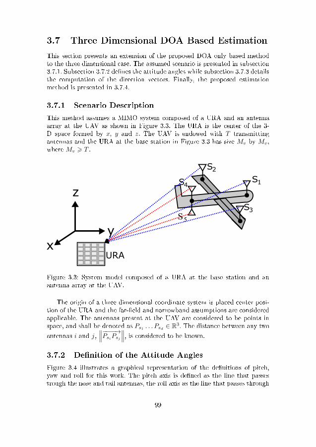
3.7 Three Dimensional DOA Based Estimation

This section presents an extension of the proposed DOA only based methodto the three dimensional case. The assumed scenario is presented in subsection3.7.1. Subsection 3.7.2 de�nes the attitude angles while subsection 3.7.3 detailsthe computation of the direction vectors. Finally, the proposed estimationmethod is presented in 3.7.4.

3.7.1 Scenario Description

This method assumes a MIMO system composed of a URA and an antennaarray at the UAV as shown in Figure 3.3. The URA is the center of the 3-D space formed by x, y and z. The UAV is endowed with T transmittingantennas and the URA at the base station in Figure 3.3 has size Mv by Mv,where Mv > T .

URA

S3

S2

S4S1

y

z

x

Figure 3.3: System model composed of a URA at the base station and anantenna array at the UAV.

The origin of a three dimensional coordinate system is placed center posi-tion of the URA and the far-�eld and narrowband assumptions are consideredapplicable. The antennas present at the UAV are considered to be points inspace, and shall be denoted as Ps1 . . . Psd ∈ R3. The distance between any two

antennas i and j,∥∥∥−−−−→PsiPsj

∥∥∥, is considered to be known.

3.7.2 De�nition of the Attitude Angles

Figure 3.4 illustrates a graphical representation of the de�nitions of pitch,yaw and roll for this work. The pitch axis is de�ned as the line that passestrough the nose and tail antennas, the roll axis as the line that passes through

99

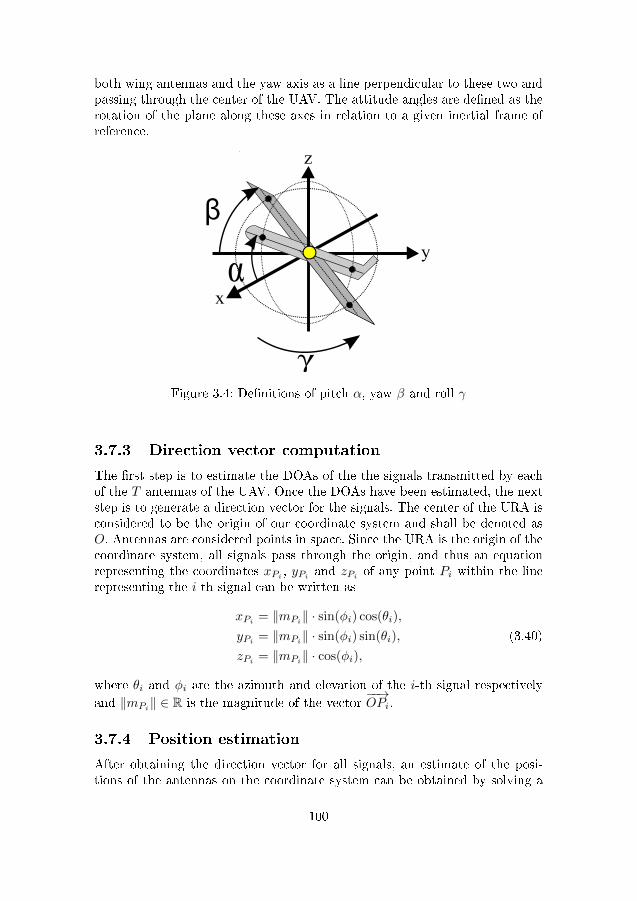
both wing antennas and the yaw axis as a line perpendicular to these two andpassing through the center of the UAV. The attitude angles are de�ned as therotation of the plane along these axes in relation to a given inertial frame ofreference.

y

z

xα

γ

β

Figure 3.4: De�nitions of pitch α, yaw β and roll γ

3.7.3 Direction vector computation

The �rst step is to estimate the DOAs of the the signals transmitted by eachof the T antennas of the UAV. Once the DOAs have been estimated, the nextstep is to generate a direction vector for the signals. The center of the URA isconsidered to be the origin of our coordinate system and shall be denoted asO. Antennas are considered points in space. Since the URA is the origin of thecoordinate system, all signals pass through the origin, and thus an equationrepresenting the coordinates xPi , yPi and zPi of any point Pi within the linerepresenting the i-th signal can be written as

xPi = ‖mPi‖ · sin(φi) cos(θi),

yPi = ‖mPi‖ · sin(φi) sin(θi), (3.40)

zPi = ‖mPi‖ · cos(φi),

where θi and φi are the azimuth and elevation of the i-th signal respectively

and ‖mPi‖ ∈ R is the magnitude of the vector−−→OPi.

3.7.4 Position estimation

After obtaining the direction vector for all signals, an estimate of the posi-tions of the antennas on the coordinate system can be obtained by solving a

100

system of equations based on the distance between each pair of antennas. TheEuclidean distance between two points A ∈ R3 and B∈ R3 is given by

m−−→AB

=√

(xA − xB)2 + (yA − yB)2 + (zA − zB)2. (3.41)

To �nd the estimate of the point where antennas i and j are located xA,xB , yA, yB , zA and zB can be replaced by xPi , xPj , yPi , yPj , zPi and zPjrespectively. Since the distances between each pair of antennas and the DOAsof each signal are known, ‖mPi‖ and

∥∥mPj

∥∥ can be obtained, yielding anestimation of the positions of antennas i and j with respect to the center ofthe URA. Note that there are n(n− 1)/2 available equations to choose from,where n is the number of antennas present at the UAV. Once the position ofthe antennas in the UAV has been calculate, the TRIAD algorithm can beused to determine its attitude. The TRIAD algorithm is detailed in AppendixH.

3.8 Simulation Results

This section presents a performance assessment of the proposed �ip-�op andjoint positioning methods. Subsection 3.8.1 presents the results obtained forsimulated data while subsection 3.8.2 presents the results obtained using mea-sured data.

3.8.1 Results for Simulated Data

The performance of the proposed �ip-�op and joint positioning algorithmsis assessed by a set of numerical simulations. The simulation assumes twoantenna subarrays at the wing mirrors; these are considered to be ULAs com-posed of M = 5 antennas with inner element spacing of ∆m = λ

2 . For thesimulations, this work assumes the transmitter is using the LTE standard,with the maximum fast Fourier transform size of 2048, of which 1200 aree�ective subcarriers, and 15 kHz subcarrier spacing. Estimations are done as-suming T = 100 OFDM symbols have been sampled with a normal cyclicpre�x. Frequency correlation is introduced by following the model proposedin [51]. To assess the performance of the proposed methods with respect tothe bandwidth of the transmitted signal, a bandwidth ranging from a tonalsignal (narrowband) to 20 MHz (largest possible LTE channel bandwidth) isconsidered. The ranging estimation is done only using the range parameterpresent in the spherical wave model, since the TDOA estimate reliability de-pends on the synchronization between transmitter and receiver. The antennaarrays are assumed to be placed 1.80 m apart from each other, the average carwidth. Unless stated otherwise, the simulations assume the presence of 3 nonline of sight (NLOS) components with respective scatterers randomly placedbetween the transmitter and the receiving array. The number of componentsis not assumed to be known for the purposed of estimating the parameters

101

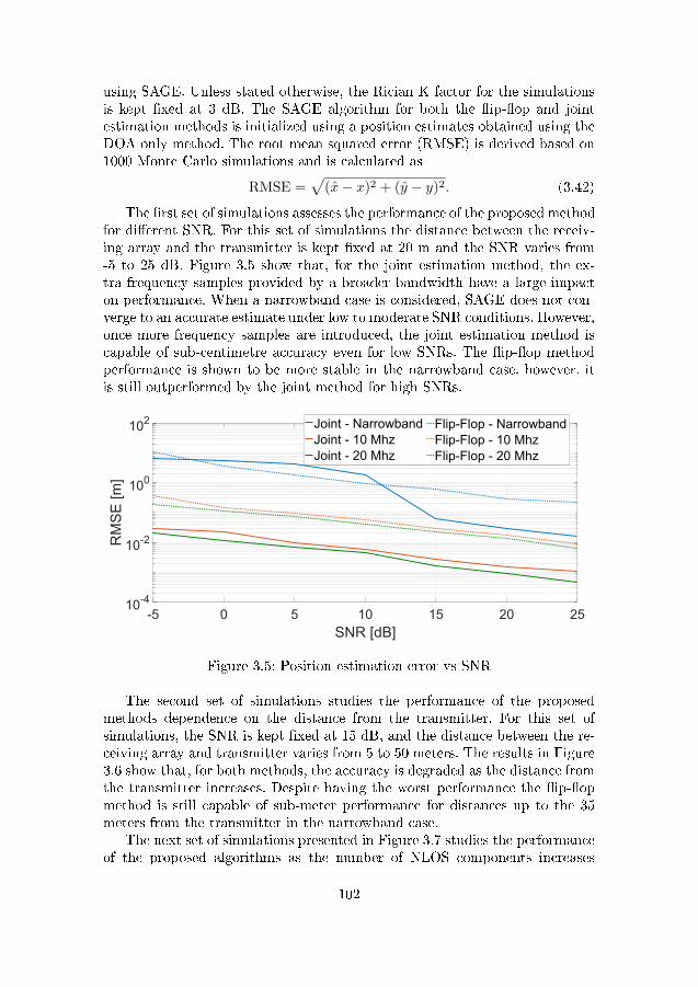
using SAGE. Unless stated otherwise, the Rician K factor for the simulationsis kept �xed at 3 dB. The SAGE algorithm for both the �ip-�op and jointestimation methods is initialized using a position estimates obtained using theDOA only method. The root mean squared error (RMSE) is derived based on1000 Monte Carlo simulations and is calculated as

RMSE =√

(x− x)2 + (y − y)2. (3.42)

The �rst set of simulations assesses the performance of the proposed methodfor di�erent SNR. For this set of simulations the distance between the receiv-ing array and the transmitter is kept �xed at 20 m and the SNR varies from-5 to 25 dB. Figure 3.5 show that, for the joint estimation method, the ex-tra frequency samples provided by a broader bandwidth have a large impacton performance. When a narrowband case is considered, SAGE does not con-verge to an accurate estimate under low to moderate SNR conditions. However,once more frequency samples are introduced, the joint estimation method iscapable of sub-centimetre accuracy even for low SNRs. The �ip-�op methodperformance is shown to be more stable in the narrowband case, however, itis still outperformed by the joint method for high SNRs.

-5 0 5 10 15 20 25

SNR [dB]

10-4

10-2

100

102

RM

SE

[m

]

Joint - Narrowband

Joint - 10 Mhz

Joint - 20 Mhz

Flip-Flop - Narrowband

Flip-Flop - 10 Mhz

Flip-Flop - 20 Mhz

Figure 3.5: Position estimation error vs SNR

The second set of simulations studies the performance of the proposedmethods dependence on the distance from the transmitter. For this set ofsimulations, the SNR is kept �xed at 15 dB, and the distance between the re-ceiving array and transmitter varies from 5 to 50 meters. The results in Figure3.6 show that, for both methods, the accuracy is degraded as the distance fromthe transmitter increases. Despite having the worst performance the �ip-�opmethod is still capable of sub-meter performance for distances up to the 35meters from the transmitter in the narrowband case.

The next set of simulations presented in Figure 3.7 studies the performanceof the proposed algorithms as the number of NLOS components increases

102

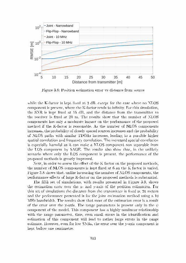
5 10 15 20 25 30 35 40 45 50Distance from transmitter [m]

10-4

10-2

100

102

RM

SE

[m]

Joint - Narrowband

Flip-Flop - Narrowband

Joint - 10 MHz

Flip-Flop - 10 MHz

Figure 3.6: Position estimation error vs distance from source

while the K-factor is kept �xed at 3 dB, except for the case where no NLOScomponent is present, where the K-factor tends to in�nity. For this simulation,the SNR is kept �xed at 15 dB, and the distance from the transmitter tothe receiver is �xed at 20 m. The results show that the number of NLOScomponents has only a moderate impact on the performance of the proposedmethod if the K-factor is reasonable. As the number of NLOS componentsincreases, the probability of closely spaced sources increases and the probabilityof NLOS paths with similar TDOAs increases, leading to a possible higherspatial correlation and frequency correlation. The increased spatial correlationis especially harmful as it can make a NLOS component non separable fromthe LOS component by SAGE. The results also show that, in the unlikelyscenario where only the LOS component is present, the performance of theproposed methods is greatly improved.

Next, in order to assess the e�ect of the K-factor on the proposed methods,the number of NLOS components is kept �xed at 6 an the K-factor is varied.Figure 3.8 shows that, unlike increasing the number of NLOS components, theperformance e�ects of large K-factor on the proposed methods is substantial.

The �fth set of simulations, with results presented in Figure 3.9, showsthe estimation error over the x- and y-axis of the position estimation. Forthis set of simulations the distance from the transmitter is �xed at 20 metersand the performance presented is for the joint estimation method using a 10MHz bandwidth. The results show that most of the estimation error is a resultof the error over the y-axis. The range parameters is present only in the ψcomponent of the model. This component has a highly nonlinear relationshipwith the range parameter, thus, even small errors in the identi�cation andestimation of this component will lead to rather large errors in the rangeestimate. However, even for low SNRs, the error over the y-axis component iskept bellow one centimetre.

103

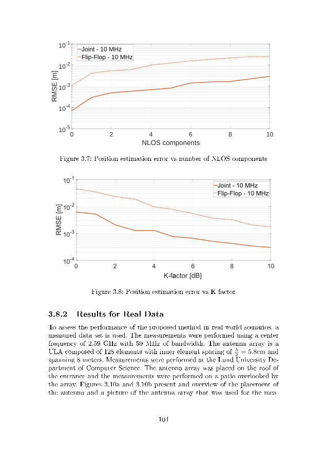
0 2 4 6 8 10NLOS components

10-5

10-4

10-3

10-2

10-1

RM

SE

[m]

Joint - 10 MHzFlip-Flop - 10 MHz

Figure 3.7: Position estimation error vs number of NLOS components

0 2 4 6 8 10

faactor [dB]K-

10-4

10-3

10-2

10-1

RM

SE

[m

]

Joint - 10 MHz

Flip-Flop - 10 MHz

Figure 3.8: Position estimation error vs K-factor

3.8.2 Results for Real Data

To assess the performance of the proposed method in real world scenarios, ameasured data set is used. The measurements were performed using a centerfrequency of 2.59 GHz with 50 MHz of bandwidth. The antenna array is aULA composed of 128 elements with inner element spacing of λ2 = 5.8cm andspanning 8 meters. Measurements were performed at the Lund University De-partment of Computer Science. The antenna array was placed on the roof ofthe entrance and the measurements were performed on a patio overlooked bythe array. Figures 3.10a and 3.10b present and overview of the placement ofthe antenna and a picture of the antenna array that was used for the mea-

104

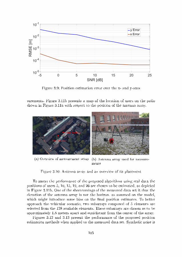
-5 0 5 10 15 20 25

SNR [dB]

10-5

10-4

10-3

10-2

10-1

RM

SE

[m

]y Error

x Error

Figure 3.9: Position estimation error over the x- and y-axes

surements. Figure 3.11b presents a map of the location of users on the patioshown in Figure 3.11a with respect to the position of the antenna array.

Antenna array

User locations

(a) Overview of measurement setup (b) Antenna array used for measure-ments

Figure 3.10: Antenna array and an overview of its placement

To assess the performance of the proposed algorithms using real data thepositions of users 5, 10, 15, 19, and 26 are chosen to be estimated, as depictedin Figure 3.11b. One of the shortcomings of the measured data set it that theelevation of the antenna array is not the horizon, as assumed on the model,which might introduce some bias on the �nal position estimates. To betterapproach the vehicular scenario, two subarrays composed of 5 elements areselected from the 128 avaliable elements. These subarrays are chosen as to beapproximately 1.8 meters apart and equidistant from the center of the array.

Figures 3.12 and 3.13 present the performance of the proposed positionestimation methods when applied to the measured data set. Synthetic noise is

105

(a) Patio where measurements wereperformed

Ante

nna A

rray

(b) User distribution for measure-ments

Figure 3.11: Patio where measurements were performed and map of user dis-tribution

added to the measurements in order to assess the performance of the proposedmethod with respect to SNR in real scenarios. The results show that, for user5, there is a constant bias present in the estimation. This is due to the fact thatuser 5 has a very low elevation angle with respect to the antenna array, thiswill lead to the measurements not �tting the assumed model. Furthermore, theantenna responses for such a low elevation angle can be very di�erent from theassumed isometric patterns. For the remaining users the performance behavessimilarly to the results obtained with the simulated data set, users that arelocated further form the array will have a smaller localization accuracy thanthose closer to the array.

The overall di�erence in performance from the real data set to the simulateddata set is most likely due to noise already present in the measurements andwhich is introduced by instruments such as power ampli�ers and convertersused in the set-up. Despite these imprecisions, the proposed joint estimationmethod was capable of achieving sub meter performance for an added SNRof up to 10 dB for all except user 5, and presented centimetre-level accuracyfor a SNR of 20 dB. The �ip-�op method was also able to achieve sub-meteraccuracy for SNRs larger than 10 dB with a faster convergence rate whencompared to the joint method.

106

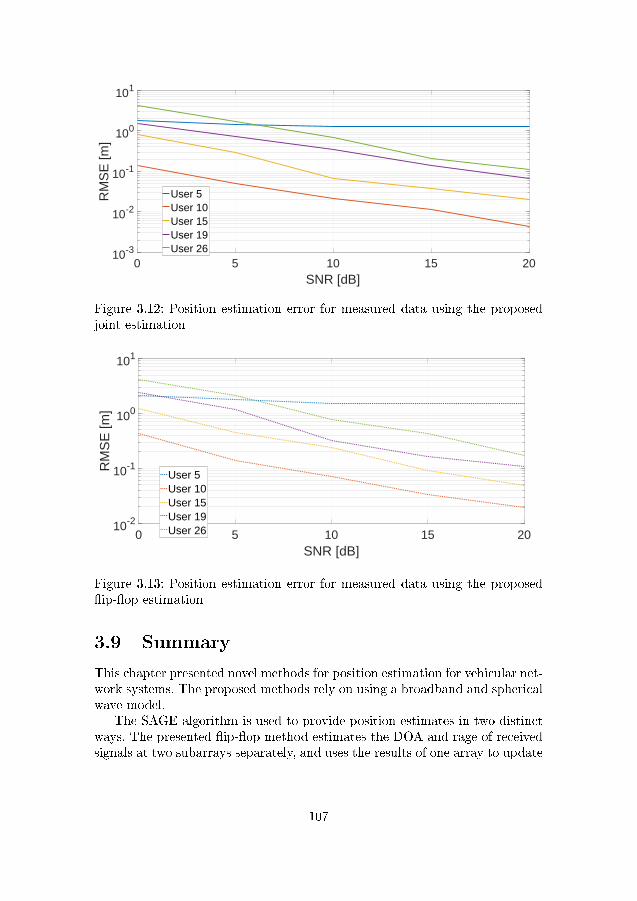
0 5 10 15 20SNR [dB]

10-3

10-2

10-1

100

101

RM

SE

[m]

User 5User 10User 15User 19User 26

Figure 3.12: Position estimation error for measured data using the proposedjoint estimation

0 5 10 15 20SNR [dB]

10-2

10-1

100

101

RM

SE

[m]

User 5User 10User 15User 19User 26

Figure 3.13: Position estimation error for measured data using the proposed�ip-�op estimation

3.9 Summary

This chapter presented novel methods for position estimation for vehicular net-work systems. The proposed methods rely on using a broadband and sphericalwave model.

The SAGE algorithm is used to provide position estimates in two distinctways. The presented �ip-�op method estimates the DOA and rage of receivedsignals at two subarrays separately, and uses the results of one array to update

107

the problem on the remaining one. This method has moderate accuracy and afast convergence time.

The proposed joint estimation method is used to obtain a direct estimateof the coordinates of the transmitter by parametrizing the problem directlyover such coordinates. While this method has a slower convergence time, it iscapable of providing superior performance compared to the �ip-�op method.

The performance of the proposed methods is studied using simulated andreal measured data. Using the simulated data set this work shows that theproposed methods are capable of sub centimetre level accuracy when the onlyerror source is additive white Gaussian noise. In case of using the real data setthis work proves that the proposed method is capable of achieving centimetre-level accuracy for moderate distances and large SNRs, and will provide submeter accuracy for moderate SNRs when other sources of error are introducedby the measurement chain.

The proposed methods can be used as a stand-alone localization estimationmethods as well as for spoo�ng mitigation, as they rely solely on estimatingparameters from the physical layer. Such parameters are extremely hard tofake with hardware available today. Furthermore, they do not require anyspeci�c data to be transmitted and can be applied when any data exchange ishappening on the network. Therefore, the proposed methods do not imply anincreased network load.

108

Conclusion

In this work the following research questions were tackled:

1. How to estimate the directions of arrival of correlated sources that areimpinging on an antenna array that does not possess the necessary char-acteristics (geometry or electromagnetic response) for doing so?

2. Can array processing techniques be used to provide improved lifetimeand communication performance in wireless sensor network?

3. Can array processing techniques be used to reliably estimate positionof vehicles and pedestrians in vehicular scenarios based on their radiotransmissions?

The �rst research question was addressed in Chapter 1. This chapter dis-cussed two approaches for sector detection and discretization, one approachis based on the UT while the other is based on the PCA. The presented ap-proaches aim to preserve the statistical characteristics of the signal to be trans-formed while minimizing the transformation bias introduced in the process.

Linear array interpolation was discussed and an extension of linear inter-polation to the multidimensional case was presented. The approach generalizesthe problem of linear interpolation to an arbitrary number of dimensions andallows the application of linear interpolation to arrays other than linear.

Two di�erent alternatives for nonlinear array interpolation were also pre-sented in Chapter 1. A way of performing array interpolation using the MARSmethod was presented. MARS is capable of expressing non-linear relationshipsbetween the real and the desired response. MARS is shown to achieve goodperformance for larger SNRs and can provide performances close to the CRLB.Furthermore, a novel approach for array interpolation extending GRNNs tothe problem of array interpolation was also presented. Using GRNNs allowsthe interpolation to take into account larger sectors of the �eld of view of theantenna array and to achieve DOA estimation results with smaller estimationerror compared to standard linear array interpolation. The proposed method isspecially bene�cial for arrays with a limited number of elements or in the casewhere a larger number of signals is present at the array, since in these casesthe transformation error for the linear approach will lead to considerable bias

109

in the DOA estimation. As it is possible to implement the proposed GRNNarray interpolation in a parallel manner, this leads to a fast interpolation espe-cially suitable for real time applications. While nonlinear methods are capableof providing an improvement of the linear interpolation, it is computationallyexpensive and does not always provide a large improvement.

The performance of the proposed nonlinear interpolation methods was as-sessed using the response obtained from a real array. For such array, the pro-posed nonlinear methods were capable of vastly outperforming their linearcouterpart.

The second research question was addressed in Chapter 2, which presents aframework for tackling practical problems for the implementation of C-MIMOin WSNs. The energy e�ciency of C-MIMO in relation to that of multihopcommunications were studied and expressions comparing the consumption ofmulti-hop and C-MIMO are derived. This allows a routing mechanism to prop-erly decide when to employ multi-hop or C-MIMO, achieving the minimalpossible energy consumption for data transmission.

A method allowing the various nodes involved in C-MIMO to properlyschedule transmission and reception was presented. A simple sliding correlatorsynchronization method was also presented as means of achieving coarse syn-chronization. More precise synchronization methods based on ML and a DFTwere presented. It was shown that the ML method is capable of achieving ahigher degree of accuracy, whereas the DFT based method is computationallyless complex. Furthermore, an analysis of the e�ect of synchronization errorson C-MIMO schemes and of how the synchronization errors spread over thenetwork was presented. Based on this analysis, a relation between symbol pe-riods, clock drift, and synchronization error was derived. This can be used toensure that an acceptable degree of synchronization is achieved for a givendata rate by using C-MIMO.

Also in Chapter 2, a method that allows the formation of e�cient C-MIMOcluster was proposed, availing the bene�ts provided by this communicationscheme, such as reduced energy cost and better distribution of energy de-mand. The proposed method was shown to extend network lifetime by reduc-ing individual node failures and to achieve networks with a more homogeneousdistribution of energy between the nodes, resulting in networks that remainfully connected for longer periods.

The last research question was addressed in Chapter 3, where two di�erentmethods for position estimation in vehicular networks were presented. Thesemethods rely on the presence of separate antenna arrays on the frame of thevehicle and use a spherical wave model in order to estimate the position of atransmitter.

A fast converging �ip-�op method that performs estimations of DOA andrage at each subarray individually was presented. This method uses the outputof the estimation at each subarray to update the estimation problem on theremaining subarray. A joint estimation method, that uses the data of both

110

subarrays simultaneously to estimate the coordinates of the transmitter di-rectly was also presented. This method is capable of superior accuracy whencompared to the �ip-�op method at the cost of increased convergence time.

Both methods were tested using simulated and a real measured data set.The simulated data shows that the proposed methods are capable of centimetrelevel accuracy under ideal conditions. The real data set shows that the pro-posed methods are still capable of achieving sub metre accuracy when othersources of error, such as the ones introduced by conversion and ampli�cation,are present.

In summary, this work aimed to bring array processing closer to real lifeproblems. Array interpolation allows the application, in real systems, of signalprocessing tools that were previously con�ned to theory. Cooperative MIMOcan be of great use to WSNs to extend their lifetime and, with that, theirusability. Finally, array processing can be used to help solve the problem oflocalization in the context of vehicular networks, solving the problem of relia-bility that is present when GPS or RSSI information is used. This can enableimportant technologies such as automated driving and platooning to becomea reality.

111

Author's Publications

[ath1] S. Caizzone, W. Elmarissi, M. A. M. Marinho, and F. Antreich. Di-rection of arrival estimation performance for compact antenna arrayswith adjustable size. The IEEE International Microwave Symposium(IMS2017), 2017.

[ath2] E. P. de Freitas, R. K. Miranda, M. A. M. Marinho, J. P. C. L. da Costa,and C. E. Pereira. A practical implementation of a cooperative antennaarray for wireless sensor networks. In Conference on Smart Spaces,pages 309�318. Springer, 2015.

[ath3] E. P. Freitas, J. P. C. L. Costa, A. L. F. Almeida, and M. A. M. Mar-inho. Applying MIMO techniques to minimize energy consumption forlong distances communications in wireless sensor networks. In Springer-Verlag, editor, NEW2AN/ruSMART 2012, pages 379�390, 2012.

[ath4] J. Milanezi Jr, J. P. C. L. da Costa, R. S. Ferreira Junior, M. A. M.Marinho, R. A. Shayani, and R. T. de Sousa Júnior. Energy harvestingphotovoltaic system to charge a cell phone in indoor environments. InInternational Conference on Composite Materials & Renewable EnergyApplications 2014, 2014.

[ath5] R. S. Ferreira Jr., M. A. M. Marinho, K. Liu, J. P. C. L. da Costa, A. V.Amaral, and H. C. So. Improved landing radio altimeter for unmannedaerial vehicles based on an antenna array. 2012.

[ath6] J. P. A. Maranhão, J. P. C. L. da Costa, E. P. de Freitas, M. A. M.Marinho, and G. Del Galdo. Multi-hop cooperative XIXO transmissionscheme for delay tolerant wireless sensor networks. In Smart Antennas(WSA 2016); Proceedings of the 20th International ITG Workshop on,pages 1�5. VDE, 2016.

[ath7] M. A. M. Marinho, F. Antreich, S. Caizzone, J. P. C. L. da Costa,A. Vinel, and E. P. de Freitas. Robust nonlinear array interpolationfor direction of arrival estimation of highly correlated signals. SignalProcessing, 144:19�28, 2018.

113

[ath8] M. A. M. Marinho, F. Antreich, and J. P. C. L. da Costa. Improvedarray interpolation for reduced bias in DOA estimation for gnss. In TheInstitute of Navigation, International Technical Meeting (ION ITM)2014, 2014.

[ath9] M. A. M. Marinho, F. Antreich, J. P. C. L. da Costa, and J. A. Nossek.Reduced rank tls array interpolation for DOA estimation. In 18th In-ternational ITG Workshop on Smart Antennas (WSA 2014), 2014.

[ath10] M. A. M. Marinho, F. Antreich, J. P. C. L. da Costa, and J. A. Nossek.A signal adaptive array interpolation approach with reduced transfor-mation bias for DOA estimation of highly correlated signals. In Acous-tics, Speech, and Signal Processing, 2004. Proceedings. (ICASSP '14).IEEE International Conference on, 2014.

[ath11] M. A. M. Marinho, J. P. C. L. da Costa, F. Antreich, A. L. F.de Almeida, G. Del Galdo, E. P. de Freitas, and A. Vinel. Array in-terpolation based on multivariate adaptive regression splines. In Sen-sor Array and Multichannel Signal Processing Workshop (SAM), 2016IEEE, pages 1�5. IEEE, 2016.

[ath12] M. A. M. Marinho, J. P. C. L. da Costa, F. Antreich, E. P. de Freitas,and A. Vinel. Adaptive communication and cooperative MIMO clusterformation for improved lifetime in wireless sensor networks. In 2016IEEE International Conference on Wireless for Space and Extreme En-vironments (WiSEE), Aachen, Germany, September 26-29, 2016, 2016.

[ath13] M. A. M. Marinho, J. P. C. L. da Costa, F. Antreich, and L. R. A. X.de Menezes. Unscented transformation based array interpolation. InProc. 40th International Conference on Acoustics, Speech, and SignalProcessing (ICASSP), Brisbane, Australia, April 2015.

[ath14] M. A. M. Marinho, J. P. C. L. da Costa, F.Antreich, and L. R. A. X.de Menezes. Multidimensional array interpolation applied to directionof arrival estimation. In 19th International ITG Workshop on SmartAntennas (WSA 2015), 2015.

[ath15] M. A. M. Marinho, E. P. de Freitas, J. P. C. L. da Costa, A. L. F.de Almeida, and R. T. de Sousa Jr. Using cooperative MIMO tech-niques and UAV relay networks to support connectivity in sparse wire-less sensor networks. In Computing, Management and Telecommunica-tions (ComManTel), 2013 International Conference on, 2013.

[ath16] M. A. M. Marinho, E. P. de Freitas, J. P. C. L. da Costa, A. L. F.de Almeida, and R. T. de Sousa Jr. Using MIMO techniques to enhancecommunication among static and mobile nodes in wireless sensor net-works. In Advanced Information Networking and Applications (AINA),2013 IEEE 27th International Conference on, 2013.

114

[ath17] M. A. M. Marinho, E. P. de Freitas, J. P. C. L. da Costa, and R. T.de Sousa Jr. Applying cooperative MIMO technique in an adaptiverouting mechanism for wireless sensor networks. In 2013 IEEE Confer-ence on Wireless Sensors (ICWiSe2013), 2013.

[ath18] M. A. M. Marinho, E. P. de Freitas, J. P. C. L. da Costa, and R. T.de Sousa Jr. Synchronization for cooperative MIMO in wireless sensornetworks. In NEW2AN/ruSMART 2013, 2013.

[ath19] M. A. M. Marinho, E. P. de Freitas, J. P. C. L. da Costa, and R. T.de Sousa Jr. Sensor localization via diversely polarized antennas. InInternational Workshop on Performance Control in Wireless SensorNetworks (PWSN), 2014.

[ath20] M. A. M. Marinho, R. S. Ferreira Jr., J. P.C. L. da Costa, E. P. de Fre-itas, K. Liu, H. C. So, and F. Antreich. Antenna array based positioningscheme for unmanned aerial vehicles. In 17th International ITG Work-shop on Smart Antennas (WSA 2013), 2013.

[ath21] M. A. M. Marinho, A. Vinel, F. Antreich, J. P. C. L. da Costa, andE. P. de Freitas. Antenna array based localization scheme for vehicularnetworks. In Computer and Information Technology (CIT), 2017 IEEEInternational Conference on, pages 142�146. IEEE, 2017.

[ath22] R. K. Miranda, J. P. C. L. da Costa, M. A. M. Marinho, E. P. de Fre-itas, and R. T. de Sousa Jr. Evaluation of space-time-frequency (stf)-coded MIMO-OFDM systems in realistic channel models. In 28th IEEEInternational Conference on Advanced Information Networking and Ap-plications (AINA-2014), 2014.

115

References

[1] I. F. Akyildiz, W. Su, Y. Sankarasubramaniam, and E. Cayirci. Wirelesssensor networks: A survey. Computer Networks, 38:393�422, 2002.(Cited on pages 53 and 1)

[2] K. P. Ang, L.and Seng, L. W. Chew, L. S. Yeong, andW. C. Chia.WirelessMultimedia Sensor Networks on Recon�gurable Hardware: InformationReduction Techniques. Springer Science & Business Media, 2013.(Cited on pages 63 and 58)

[3] A. J. Barabell. Improving the resolution performance of eigenstructuredbased direction-�nding algorithms. In Proceedings of ICASSP 83, 1983.(Cited on pages 8, 9, 19, 11, and 22)

[4] M. S. Bartlett. Smoothing periodograms from time series with continuousspectra. Nature, 161:686�687, 1948.(Cited on pages 8, 9, 23, 10, 25, and 32)

[5] C. Bettstetter. On the minimum node degree and connectivity of a wire-less multihop network. In Proceedings of the 3rd ACM international sym-posium on Mobile ad hoc networking & computing, pages 80�91. ACM,2002.(Cited on pages 78 and 73)

[6] M. Bhardwaj and A. P. Chandrakasan. Upper bounds on the lifetime ofsensor networks. In Proceedings of IEEE ICC01, 2001.(Cited on page 60)

[7] M. Biguesh and A. B. Gershman. Training-based MIMO channel estima-tion: A study of estimator tradeo�s and optimal training signals. IEEETransactions on Signal Processing, 54:884�893, 2006.(Cited on pages 57 and 55)

[8] H. Black. A passive system for determining the attitude of a satellite.AIAA Journal, 2:1350�1351, July 1964.(Cited on page 151)

117

[9] H. Black. Early developments of transit, the navy navigation satellitesystem. Journal of Guidance, Control and Dynamics, 13:577�585, July1990.(Cited on page 151)

[10] Y. Bresler and A. Macovski. Exact maximum likelihood estimation of su-perimposed exponentials signals in noise. IEEE ASSP Magazine, 34:1081�189, 1986.(Cited on pages 8, 9, and 11)

[11] T. P. Bronez. Sector interpolation of non-uniform arrays for e�cient highresolution bearing estimation. InAcoustics, Speech, and Signal Processing,1988. ICASSP-88., 1988 International Conference on, 1988.(Cited on pages 10, 26, 28, and 12)

[12] M. Buhren, M. Pesavento, and J. F. Bohme. A new approach to arrayinterpolation by generation of arti�cial shift invariances: Interpolated ES-PRIT. In Acoustics, Speech, and Signal Processing, 2003. Proceedings.(ICASSP '03). 2003 IEEE International Conference on, 2003.(Cited on pages 10, 15, 21, 12, 18, and 24)

[13] M. Buhren, M. Pesavento, and J. F Böhme. Virtual array design forarray interpolation using di�erential geometry. In Acoustics, Speech, andSignal Processing, 2004. Proceedings. (ICASSP '04). IEEE InternationalConference on, volume 2, 2004.(Cited on pages 10, 19, 12, and 24)

[14] S. Caizzone and A. Dreher. Miniaturized DRA array for GNSS applica-tions. In 2015 9th European Conference on Antennas and Propagation(EuCAP), pages 1�2. IEEE, 2015.(Cited on pages 44 and 45)

[15] S. Caizzone, W. Elmarissi, M. A. M. Marinho, and F. Antreich. Directionof arrival estimation performance for compact antenna arrays with ad-justable size. The IEEE International Microwave Symposium (IMS2017),2017.(Cited on page 44)

[16] J. Capon. High-resolution frequency-wavenumber spectrum analysis. Pro-ceedings IEEE, 57:1408�1418, 1969.(Cited on pages 8, 9, 23, 10, 25, and 32)

[17] C. Chen, J. Ma, and K. Yu. Designing energy-e�cient wireless sensornetworks with mobile sinks. In Sensys06, 2006.(Cited on pages 53, 59, and 1)

[18] S. Cho and A. Chandrakasan. Energy-e�cient protocols for low dutycycle wireless microsensor. In Proceedings of the 33rd Annual Hawaii

118

International Conference on System Sciences, 2000.(Cited on pages 53 and 1)

[19] P. J. Chung and J. F. Böhme. Comparative convergence analysis of EMand SAGE algorithms in DOA estimation. IEEE Transactions on SignalProcessing, 49:2940�2949, 2001.(Cited on pages 8 and 10)

[20] D. S. J. D. Couto, D. Aguayo, J. Bicket, and R. Morris. A high-throughputpath metric for multi-hop wireless routing. Wirel. Netw, 11:419�435,2005.(Cited on page 59)

[21] J. H. Cozzens and M. J. Sousa. Source enumeration in a correlated signalenvironment. IEEE Transactions on Acoustics Speech and Signal Process-ing, 42:304�317, 1994.(Cited on pages 14 and 17)

[22] S. B. Cruz, T. E. Abrudan, Z. Xiao, N. Trigoni, and J. Barros. Neighbor-aided localization in vehicular networks. IEEE Transactions on IntelligentTransportation Systems, 2017.(Cited on page 89)

[23] S. Cui and A. J. Goldsmith. Energy-e�ciency of MIMO and cooperativeMIMO techniques in sensor networks. IEEE Journal on Selected Areas inCommunications, 2004.(Cited on pages 53 and 2)

[24] J. P. C. L. da Costa, M. Haardt, F. Romer, and G. Del Galdo. Enhancedmodel order estimation using higher-order arrays. Conference Record ofThe Forty-First Asilomar Conference on Signals, Systems & Computers,pages 412�416, 2007.(Cited on pages 15 and 18)

[25] J. P. C. L. da Costa, K. Liu, H. C. So, F. Roemer, M. Haardt, andS. Schwarz. Generalized multidimensional prewhitening for enhanced sig-nal reconstruction and parameter estimation. In Signal Processing, Else-vier publisher, 2013.(Cited on pages 38 and 42)

[26] J. P. C. L. da Costa, F. Roemer, and M. Haardt. Deterministic prewhiten-ing to improve subspace parameter estimation techniques in severely col-ored noise environments. In Proc. 54th International Scienti�c Colloquium(IWK), 2009.(Cited on pages 38 and 42)

[27] J. P. C. L. da Costa, F. Roemer, M. Haardt, and R. T. de Sousa Jr.Multi-dimensional model order selection. EURASIP Journal on Advances

119

in Signal Processing, 26, 2011.(Cited on pages 15 and 18)

[28] J. P. C. L. da Costa, F. Roemer, M. Weis, and M. Haard. Robust R-Dparameter estimation via closed-form PARAFAC. In Proc. ITG Workshopon Smart Antennas (WSA'10), 2010.(Cited on pages 17, 38, 20, and 42)

[29] J. P. C. L. da Costa, D. Schulz, F. Roemer, M. Haardt, and J. A. Apoli-nario Jr. Robust R-D parameter estimation via closed-form PARAFAC inkronecker colored environments. In Proc. 7-th International Symposiumon Wireless Communications Systems (ISWCS 2010), 2010.(Cited on pages 17, 38, 20, and 42)

[30] V. Daiya, J. Ebenezer, S. A. V. S. Murty, and B. Raj. Experimentalanalysis of RSSI for distance and position estimation. In Recent Trendsin Information Technology (ICRTIT), 2011 International Conference on,pages 1093�1098. IEEE, 2011.(Cited on pages 72 and 67)

[31] L. M. S. De Souza, H. Vogt, and M. Beigl. A survey on fault tolerancein wireless sensor networks. Interner Bericht. Fakultät für Informatik,Universität Karlsruhe: Karlsruhe, Germany, 2007.(Cited on pages 81 and 74)

[32] A. P. Dempster, N. M. Laird, and D. B. Rubin. Maximum likelihood fromincomplete data via the EM algorithm. J. Royal Statistical Soc. B., 39(1),1977.(Cited on pages 7, 9, 33, 10, and 38)

[33] F. A. Dietrich. A tutorial on channel estimation with SAGE. TechnicalReport TUM-LNS-TR-06-03, 2006.(Cited on pages 7, 9, 33, 10, and 38)

[34] I. Dietrich and F. Dressler. On the lifetime of wireless sensor networks.ACM Transactions on Sensor Networks, 5, 2009.(Cited on pages 53 and 1)

[35] P. Dollar, C. Wojek, B. Schiele, and P. Perona. Pedestrian detection: Anevaluation of the state of the art. IEEE transactions on pattern analysisand machine intelligence, 34(4):743�761, 2012.(Cited on page 88)

[36] J. Elson, L. Girod, and D. Estrin. Fine-grained network time synchroniza-tion using reference broadcasts. In Proceedings of the Fifth Symposiumon Operating Systems Design and Implementation, 2002.(Cited on pages 64 and 59)

120

[37] J. E. Evans, J. R. Johnson, and D. F. Sun. Application of advanced signalprocessing techniques to angle of arrival estimation in ATC navigation andsurveillance system. Technical report, 1982.(Cited on pages 8, 14, 11, and 16)

[38] J. A. Fessler and A. O. Hero. Space-alternating generalized expectation-maximization algorithm. IEEE Transactions on Signal Processing, 42(10),October 1994.(Cited on pages 7, 9, 33, 10, and 38)

[39] B. Friedlander. The root-MUSIC algorithm for direction �nding withinterpolated arrays. Signal Processing, 30:15�29, 1993.(Cited on pages 10, 19, 12, and 24)

[40] B. Friedlander and A. J. Weiss. Direction �nding using spatial smoothingwith interpolated arrays. Aerospace and Electronic Systems, IEEE Trans-actions on, 28:574�587, 1992.(Cited on pages 10, 33, 12, and 38)

[41] J. H. Friedman. Multivariate adaptive regression splines. The annals ofstatistics, pages 1�67, 1991.(Cited on pages 143, 144, 4, 113, and 114)

[42] S. Ganeriwal, D. Ganesan, H. Shim, V. Tsiatsis, and B. Srivastava. Es-timating clock uncertainty for e�cient duty-cycling in sensor networks.In Proceedings of the Third International Conference on Embedded Net-worked Sensor Systems (Sensys), 2005.(Cited on pages 64 and 59)

[43] S. Ganeriwal, R. Kumar, and M. B. Srivastava. Timing-sync protocol forsensor networks. In Proceedings of the Sensys03, 2003.(Cited on pages 64 and 59)

[44] D. Ganesan, R. Govindan, S. Shenker, and D. Estrin. Highly-resilient,energy-e�cient multipath routing in wireless sensor networks. ACMSIGMOBILE Mobile Computing and Communications Review, 5(4):1125,2001.(Cited on pages 53 and 1)

[45] D. M. Gavrila, J. Giebel, and S. Munder. Vision-based pedestrian de-tection: The protector system. In Intelligent Vehicles Symposium, 2004IEEE, pages 13�18. IEEE, 2004.(Cited on page 88)

[46] A. M. Geronimo, D.and Lopez, A. D. Sappa, and T. Graf. Survey of pedes-trian detection for advanced driver assistance systems. IEEE transactionson pattern analysis and machine intelligence, 32(7):1239�1258, 2010.(Cited on page 88)

121

[47] M. Haardt. E�cient one-, two- and multidimensional high-resolution ar-ray signal processing. In 3-8265-2220-6, Aachen, Germany, 1996. ShakerVerlag.(Cited on page 15)

[48] M. Haardt, F. Roemer, and G. Del Gado. Higher-order SVD basedsubspace estimation to improve parameter estimation accuracy in multi-dimensional harmonic retrieval problems. IEEE Transactions on SignalProcessing, 56(7):3198�3213, July 2008.(Cited on pages 38 and 42)

[49] A. Habibovic and J. Davidsson. Requirements of a system to reduce car-to-vulnerable road user crashes in urban intersections. Accident Analysis& Prevention, 43(4):1570�1580, 2011.(Cited on page 88)

[50] W. R. Heinzelman, A. Chandrakasan, and H. Balakrishnan. Energy-e�cient communication protocol for wireless microsensor networks. InProceedings of the 33rd Hawaii International Conference on System Sci-ences, 2000.(Cited on pages 53 and 1)

[51] P. Hoeher. A statistical discrete-time model for the wssus multipath chan-nel. IEEE Transactions on vehicular technology, 41(4):461�468, 1992.(Cited on page 101)

[52] S. M. R. Hosseini and M. A. Sebt. Array interpolation using covariancematrix completion of minimum-size virtual array. IEEE Signal ProcessingLetters, 24(7):1063, 2017.(Cited on pages 10 and 12)

[53] R. S. Ferreira Jr., M. A. M. Marinho, K. Liu, J. P. C. L. da Costa, A. V.Amaral, and H. C. So. Improved landing radio altimeter for unmannedaerial vehicles based on an antenna array. 2012.(Cited on pages 7 and 10)

[54] S. J. Julier and J. K. Uhlmann. A new extension of the Kalman �lter tononlinear systems. In Int. symp. aerospace/defense sensing, simul. andcontrols, volume 3, pages 3�2. Orlando, FL, 1997.(Cited on pages 26, 4, and 28)

[55] M. Khurana, C. Ramakrishna, and S. N. Panda. Capacity enhancementusing MU-MIMO in vehicular ad hoc network. International Journal ofApplied Engineering Research, 12(16):5872�5883, 2017.(Cited on page 89)

[56] N. Kim, Y. Lee, and H. Park. Performance analysis of MIMO system withlinear MMSE receiver. Wireless Communications, IEEE Transactions on,

122

7(11):4474�4478, 2008.(Cited on pages 57 and 55)

[57] T. King, H. Füÿler, M. Transier, and W. E�elsberg. Dead-reckoningfor position-based forwarding on highways. In Proc. of the 3rd Inter-national Workshop on Intelligent Transportation (WIT 2006), pages 199�204, 2006.(Cited on pages 89 and 3)

[58] D. Kosmanos, N. Prodromou, A. Argyriou, L. A. Maglaras, and H. Jan-icke. MIMO techniques for jamming threat suppression in vehicular net-works. Mobile Information Systems, 2016, 2016.(Cited on page 89)

[59] H. Krim and M. Viberg. Two decades of array signal processing research:The parametric approach. IEEE Signal Processing Magazine, 13:67�94,1996.(Cited on pages 7, 14, and 17)

[60] V. Kumar, S. Mishra, and N. Chand. Applications of VANETs: Present& future. Communications and Network, 5(01):12, 2013.(Cited on pages 88 and 3)

[61] T. Kurpjuhn, M. T. Ivrlac, and J. A. Nossek. Vandermonde invariancetransformation. In Acoustics, Speech, and Signal Processing, 2001. Pro-ceedings. (ICASSP '01). 2001 IEEE International Conference on, 2001.(Cited on pages 9, 17, 12, and 20)

[62] Erik G Larsson, Ove Edfors, Fredrik Tufvesson, and Thomas L Marzetta.Massive MIMO for next generation wireless systems. IEEE Communica-tions Magazine, 52(2):186�195, 2014.(Cited on page 7)

[63] B. K. Lau, G. J. Cook, and Y. H. Leung. An improved array interpo-lation approach to DOA estimation in correlated signal environments.In Acoustics, Speech, and Signal Processing, 2004. Proceedings. (ICASSP'04). IEEE International Conference on, 2004.(Cited on pages 10, 21, 12, and 24)

[64] B. K. Lau, M. Viberg, and Y. H. Leung. Data-adaptive array interpola-tion for DOA estimation in correlated signal environments. In Acoustics,Speech, and Signal Processing, 2005. Proceedings. (ICASSP '05). IEEEInternational Conference on, 2005.(Cited on pages 10, 21, 12, and 24)

[65] T. Leinmuller, E. Schoch, and F. Kargl. Position veri�cation approachesfor vehicular ad hoc networks. IEEE Wireless Communications, 13(5):16�21, 2006.(Cited on pages 89 and 3)

123

[66] P. Lettieri and M. B. Srivastava. Adaptive frame length control for im-proving wireless link throughput, range and energy e�ciency. In INFO-COM '98. Seventeenth Annual Joint Conference of the IEEE Computerand Communications Societies. Proceedings. IEEE, 1998.(Cited on pages 53 and 1)

[67] K. Lin, J. Luo, L. Hu, M. S. Hossain, and A. Ghoneim. Localization basedon social big data analysis in the vehicular networks. IEEE Transactionson Industrial Informatics, 13(4):1932�1940, 2017.(Cited on page 89)

[68] C. Liu, P. P. Vaidyanathan, and P. Pal. Coprime coarray interpolationfor DOA estimation via nuclear norm minimization. In Circuits and Sys-tems (ISCAS), 2016 IEEE International Symposium on, pages 2639�2642.IEEE, 2016.(Cited on pages 10 and 12)

[69] W. Lou, W. Liu, and Y Zhang. Performance optimization using multi-path routing in mobile ad hoc and wireless sensor networks. Combinator.Optim. Commun. Netw., 2:117�146, 2006.(Cited on page 59)

[70] D. Lucarelli and I.-J. Wang. Decentralized synchronization protocols withnearest neighbor communication. In Proceedings of the Sensys04, 2004.(Cited on pages 64 and 59)

[71] J. Mannermaa, K. Kalliomaki, T. Mansten, and S. Turunen. Timing per-formance of varios GPS receivers. In Proceedings of the 1999 Joint Meetingof the European Frequency and Time Forum and the IEEE InternationalFrequency Control Symposium, 1999.(Cited on pages 64 and 59)

[72] M. A. M. Marinho, F. Antreich, J. P. C. L. da Costa, and J. A. Nossek.A signal adaptive array interpolation approach with reduced transforma-tion bias for DOA estimation of highly correlated signals. In Acoustics,Speech, and Signal Processing, 2004. Proceedings. (ICASSP '14). IEEEInternational Conference on, 2014.(Cited on pages 44, 45, 46, and 47)

[73] M. A. M. Marinho, J. P. C. L. da Costa, F. Antreich, A. L. F. de Almeida,G. Del Galdo, E. P. de Freitas, and A. Vinel. Array interpolation based onmultivariate adaptive regression splines. In Sensor Array and Multichan-nel Signal Processing Workshop (SAM), 2016 IEEE, pages 1�5. IEEE,2016.

[74] M. A. M. Marinho, J. P. C. L. da Costa, F. Antreich, and L. R. A. X.de Menezes. Unscented transformation based array interpolation. In Proc.

124

40th International Conference on Acoustics, Speech, and Signal Processing(ICASSP), Brisbane, Australia, April 2015.(Cited on page 10)

[75] M. A. M. Marinho, J. P. C. L. da Costa, F.Antreich, and L. R. A. X.de Menezes. Multidimensional array interpolation applied to direction ofarrival estimation. In 19th International ITG Workshop on Smart Anten-nas (WSA 2015), 2015.

[76] M. A. M. Marinho, E. P. de Freitas, J. P. C. L. da Costa, A. L. F.de Almeida, and R. T. de Sousa Jr. Using cooperative MIMO techniquesand UAV relay networks to support connectivity in sparse wireless sensornetworks. In Computing, Management and Telecommunications (Com-ManTel), 2013 International Conference on, 2013.(Cited on pages 53 and 2)

[77] M. A. M. Marinho, E. P. de Freitas, J. P. C. L. da Costa, A. L. F.de Almeida, and R. T. de Sousa Jr. Using MIMO techniques to enhancecommunication among static and mobile nodes in wireless sensor net-works. In Advanced Information Networking and Applications (AINA),2013 IEEE 27th International Conference on, 2013.(Cited on pages 53 and 2)

[78] F. L. Markley. Attitude determination using vector observations and thesingular value decomposition. In AAS/AIAA Astrodynamics SpecialistConference, 1987.(Cited on page 153)

[79] G. J. McLachlan and T. Krishnan. The Em Algorithm and Extensions.John Wiley & Sons, Inc., New York, 1997.(Cited on pages 7, 9, 33, 10, and 38)

[80] V. Mhatre and C. Rosenberg. Design guidelines for wireless sensor net-works: Communication, clustering and aggregation. In Elsevier Ad HocNetworks, 2004.(Cited on page 60)

[81] M. I. Miller and D. R. Fuhrmann. Maximum-likelhood narrow-band di-rection �nding and the EM algorithm. IEEE Transactions on AcousticsSpeech and Signal Processing, 38:1560�1577, 1990.(Cited on pages 7, 9, 33, 10, and 38)

[82] R. A. F. Mini and A. A. F. Loureiro. Energy in wireless sensor networks.In Middleware for Network Eccentric and Mobile Applications, pages 3�24. Springer, 2009.(Cited on pages 53 and 1)

125

[83] M. Modsching, R. Kramer, and K. ten Hagen. Field trial on GPS accuracyin a medium size city: The in�uence of built-up. In 3Rd workshop onpositioning, navigation and communication, pages 209�218, 2006.(Cited on pages 89 and 3)

[84] T. K. Moon. The expectation-maximization algorithm. IEEE SignalProcessing Magazine, November 1996.(Cited on pages 7, 9, 33, 10, and 38)

[85] T. Nadeem, P. Shankar, and L. Iftode. A comparative study of datadissemination models for VANETs. In Mobile and Ubiquitous Systems-Workshops, 2006. 3rd Annual International Conference on, pages 1�10.IEEE, 2006.(Cited on pages 89 and 3)

[86] B. Ottersten, M. Viberg, and T. Kailath. Analysis of subspace �tting andML techniques for parameter estimation from sensor array data. IEEETransactions on Signal Processing, 40(3), March 1992.(Cited on pages 7, 9, 33, 10, and 38)

[87] B. Ottersten, M. Viberg, P. Stoica, and A. Nehorai. Exact and largesample maximum likelihood techniques for parameter estimation and de-tection in array processing. In Radar array processing, pages 99�151.Springer, 1993.(Cited on pages 7, 9, 33, 45, and 47)

[88] R. Parker and S. Valaee. Vehicular node localization using received-signal-strength indicator. IEEE Transactions on Vehicular Technology,56(6):3371�3380, 2007.(Cited on pages 89 and 3)

[89] M. Pesavento, A. B. Gershman, and Z.-Q. Luo. Robust array interpolationusing second-order cone programming. Signal Processing Letters, 9:8�11,2002.(Cited on pages 10, 19, 26, 28, 12, and 24)

[90] S. U. Pillai and B. H. Kwon. Forward/backward spatial smoothing tech-niques for coherent signal identi�cation. IEEE Transactions on Acoustics,Speech and Signal Processing, 37:8�9, January 1989.(Cited on pages 8, 13, 11, and 16)

[91] E. Radoi and A. Quinquis. A new method for estimating the number ofharmonic components in noise with application in high resolution radar.EURASIP Journal on Applied Signal Processing, pages 1177�1188, 2004.(Cited on pages 15, 32, 44, 18, 37, and 46)

[92] G. C. Reinsel and R. P. Velu. Multivariate Reduced-rank Regression.Springer New York, 1998.(Cited on pages 32 and 37)

126

[93] R. Roy and T. Kailath. ESPRIT - estimation of signal parameters viarotation invariance techniques. IEEE Transactions on Acoustics Speechand Signal Processing, 17, 1989.(Cited on pages 8, 9, 15, 16, 19, 44, 22, and 46)

[94] F. A. Santos, A. T. Akabane, R. S. Yokoyama, A. A. F. Loureiro, and L. AVillas. A roadside unit-based localization scheme to improve positioningfor vehicular networks. In Vehicular Technology Conference (VTC-Fall),2016 IEEE 84th, pages 1�5. IEEE, 2016.(Cited on page 89)

[95] R. O. Schmidt. Multiple emitter location and signal parameter estimation.IEEE Transactions on Antennas and Propagation, 34(3), March 1986.(Cited on pages 8, 9, and 10)

[96] C. Shen, Y. Zhu, S. Zhou, and J. Jiang. On the performance of V-BLAST with zero-forcing successive interference cancellation receiver. InGlobal Telecommunications Conference, 2004. GLOBECOM'04. IEEE,volume 5, pages 2818�2822. IEEE, 2004.(Cited on pages 57 and 55)

[97] E. Shih, B. H. Calhoun, S.H. Cho, and A. P. Chandrakasan. Energy-e�cient link layer for wireless microsensor networks. In VLSI, 2001. Pro-ceedings. IEEE Computer Society Workshop on, 2001.(Cited on pages 53 and 1)

[98] E. Shih, S. Cho, N. Ickes, R. Min, A. Sinha, and A. ChandrakasanA. Wang. Physical layer driven protocol and algorithm design for energy-e�cient wireless sensor networks. In Proceedings of ACM MobiCom01,2001.(Cited on pages 53 and 1)

[99] V. Shnayder, M. Hempstead, B. Chen, G. W. Allen, and M. Welsh. Sim-ulating the power consumption of large-scale sensor network applications.In Proceedings of the 2nd international conference on Embedded networkedsensor systems, pages 188�200. ACM, 2004.(Cited on pages 63, 78, 58, and 72)

[100] M. D. Shuster. Maximum likelihood estimation of spacecraft attitude.The Journal of the Astronautical Sciences, 108:2089�2117, 2001.(Cited on page 153)

[101] P. Stoica and A. Nehorai. A novel eigenanalysis method for directionestimation. In Proceedings IEEE F., 1990.(Cited on pages 8, 9, and 11)

127

[102] D. V. A. H. G. Swaroop and J. K. Hedrick. Constant spacing strategiesfor platooning in automated highway systems. Journal of dynamic sys-tems, measurement, and control, 121(3):462�470, 1999.(Cited on pages 89 and 3)

[103] A. Triwinarko, I. Dayoub, and P. Wikanta. Using MIMO and cross layerdesign for VANETs: A review. In Signals and Systems (ICSigSys), 2017International Conference on, pages 13�18. IEEE, 2017.(Cited on page 89)

[104] D. Tse and P. Viswanath. Fundamentals of Wireless Communication.Cambridge university press, 2005.(Cited on pages 58 and 56)

[105] T. Virtanen. Monaural sound source separation by nonnegative ma-trix factorization with temporal continuity and sparseness criteria. IEEEtransactions on audio, speech, and language processing, 15(3):1066�1074,2007.(Cited on page 7)

[106] M. Wax and T. Kailath. Detection of signals by information by informa-tion theoric criteria. IEEE Transactions on Acoustics Speech and SignalProcessing, 33:387�392, 1985.(Cited on pages 15 and 18)

[107] M. Weiser, B. Welch, A. Demers, and S. Shenker. Scheduling for reducedCPU energy. In Proceedings of 1st USENIX Symposium on OperatingSystem Design and Implementation, pages 13�23, November 1994.(Cited on pages 53 and 1)

[108] A. J. Weiss and M. Gavish. The interpolated ESPRIT algorithm fordirection �nding. In Electrical and Electronics Engineers in Israel, 1991.Proceedings., 17th Convention of, 1991.(Cited on pages 21 and 24)

[109] G. Wener-Allen, G. Tewari, A. Patel, M. Welsh, and R. Nagpal. Fire�yinspired sensor network synchronicity with realistic radio e�ects. In Pro-ceedings of the Third International Conference on Embedded NetworkedSensor Systems (Sensys), 2005.(Cited on pages 64 and 59)

[110] N. Wiener. Extrapolation, interpolation and smoothing of stationarytime series. MIT Press, 1949.(Cited on pages 14 and 16)

[111] P. W. Wolniansky, G. J. Foschini, G. D. Golden, and R. A. Valenzuela.V-BLAST: An architecture for realizing very high data rates over the rich-scattering wireless channel. In Signals, Systems and Electronics, 1998.(Cited on pages 56 and 54)

128

[112] A. Woo, T. Tong, and D Culler. Taming the underlying challenges ofreliable multihop routing in sensor networks. In Proc. ACM SenSys 2003,2003.(Cited on page 59)

[113] R. Xu and F. C. M. Lau. Performance analysis for MIMO systemsusing zero forcing detector over fading channels. IEE Proceedings-Communications, 153(1):74�80, 2006.(Cited on pages 57 and 55)

[114] A. Zanella, M. Chiani, and M. Z. Win. MMSE reception and successiveinterference cancellation for MIMO systems with high spectral e�ciency.Wireless Communications, IEEE Transactions on, 4(3):1244�1253, 2005.(Cited on pages 57 and 55)

[115] X. Zhu and R. D. Murch. Performance analysis of maximum likelihooddetection in a MIMO antenna system. Communications, IEEE Transac-tions on, 50(2):187�191, 2002.(Cited on pages 57 and 55)

129

Appendices

131

Appendix A

Left Centro-HermitianMatrix

De�nition A.1. A exchange matrix Qn is de�ned as a n×n matrix with onein its anti-diagonal and zeros elsewhere

Qn =

0 0 · · · 0 10 0 · · · 1 0...

... . .. ...

...0 1 · · · 0 01 0 · · · 0 0

∈ Cn×n. (A.1)

Thus, left hand multiplication of a matrix by an exchange matrix reverses theorder of its rows while a right hand multiplication will reverse the order of itscolumns.

De�nition A.2. A matrix W ∈ Ci×j is called centro-Hermitian if

QiW∗Qj = W, (A.2)

where (·)∗ stands for complex conjugation.

De�nition A.3. A matrix W ∈ Ci×j is called left centro-Hermitian if

QiW∗ = W⇔ QiW = W∗ (A.3)

133

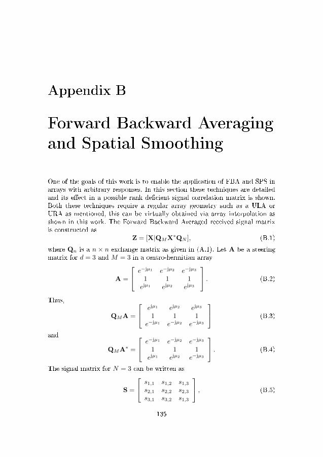
Appendix B

Forward Backward Averagingand Spatial Smoothing

One of the goals of this work is to enable the application of FBA and SPS inarrays with arbitrary responses. In this section these techniques are detailedand its e�ect in a possible rank de�cient signal correlation matrix is shown.Both these techniques require a regular array geometry such as a ULA orURA as mentioned, this can be virtually obtained via array interpolation asshown in this work. The Forward Backward Averaged received signal matrixis constructed as

Z = [X|QMX∗QN ], (B.1)

where Qn is a n × n exchange matrix as given in (A.1). Let A be a steeringmatrix for d = 3 and M = 3 in a centro-hermitian array

A =

e−jµ1 e−jµ2 e−jµ3

1 1 1ejµ1 ejµ2 ejµ3

. (B.2)

Thus,

QMA =

ejµ1 ejµ2 ejµ3

1 1 1e−jµ1 e−jµ2 e−jµ3

(B.3)

and

QMA∗ =

e−jµ1 e−jµ2 e−jµ3

1 1 1ejµ1 ejµ2 e−jµ3

. (B.4)

The signal matrix for N = 3 can be written as

S =

s1,1 s1,2 s1,3

s2,1 s2,2 s2,3

s3,1 s3,2 s1,3

, (B.5)

135

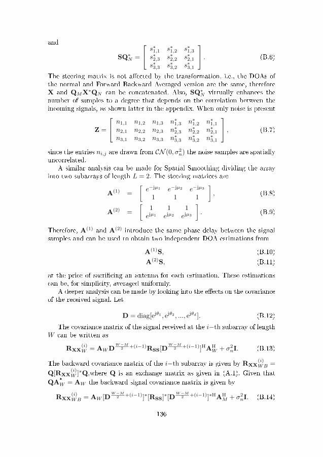
and

SQ∗N =

s∗1,1 s∗1,2 s∗1,3s∗2,3 s∗2,2 s∗2,1s∗3,3 s∗3,2 s∗3,1

. (B.6)

The steering matrix is not a�ected by the transformation, i.e., the DOAs ofthe normal and Forward Backward Averaged version are the same, thereforeX and QMX∗QN can be concatenated. Also, SQ∗N virtually enhances thenumber of samples to a degree that depends on the correlation between theincoming signals, as shown latter in the appendix. When only noise is present

Z =

n1,1 n1,2 n1,3 n∗1,3 n∗1,2 n∗1,1n2,1 n2,2 n2,3 n∗2,3 n∗2,2 n∗2,1n3,1 n3,2 n3,3 n∗3,3 n∗3,2 n∗3,1

, (B.7)

since the entries ni,j are drawn from CN (0, σ2n) the noise samples are spatially

uncorrelated.A similar analysis can be made for Spatial Smoothing dividing the array

into two subarrays of length L = 2. The steering matrices are

A(1) =

[e−jµ1 e−jµ2 e−jµ3

1 1 1

], (B.8)

A(2) =

[1 1 1ejµ1 ejµ2 ejµ3

]. (B.9)

Therefore, A(1) and A(2) introduce the same phase delay between the signalsamples and can be used to obtain two independent DOA estimations from

A(1)S, (B.10)

A(2)S, (B.11)

at the price of sacri�cing an antenna for each estimation. These estimationscan be, for simplicity, averaged uniformly.

A deeper analysis can be made by looking into the e�ects on the covarianceof the received signal. Let

D = diag[ejθ1 , ejθ2 , ..., ejθd ]. (B.12)

The covariance matrix of the signal received at the i−th subarray of lengthW can be written as

RXX(i)W = AWD

W−M2 +(i−1)RSS[D

W−M2 +(i−1)]HAH

W + σ2nI. (B.13)

The backward covariance matrix of the i−th subarray is given by RXX(i)WB =

Q[RXX(i)W ]∗Q,where Q is an exchange matrix as given in (A.1). Given that

QA*W = AW the backward signal covariance matrix is given by

RXX(i)WB = AW [D

W−M2 +(i−1)]∗[RSS]∗[D

W−M2 +(i−1)]∗HAH

M + σ2nI. (B.14)

136

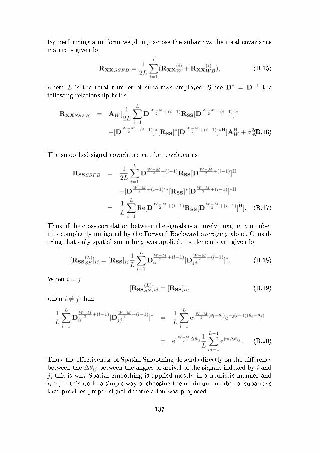
By performing a uniform weighting across the subarrays the total covariancematrix is given by

RXXSSFB =1

2L

L∑i=1

(RXX(i)W + RXX

(i)WB), (B.15)

where L is the total number of subarrays employed. Since D∗ = D−1 thefollowing relationship holds

RXXSSFB = AW [1

2L

L∑i=1

DW−M

2 +(i−1)RSS[DW−M

2 +(i−1)]H

+[DW−M

2 +(i−1)]∗[RSS]∗[DW−M

2 +(i−1)]∗H]AHW + σ2

nI.(B.16)

The smoothed signal covariance can be rewritten as

RSSSSFB =1

2L

L∑i=1

DW−M

2 +(i−1)RSS[DW−M

2 +(i−1)]H

+[DW−M

2 +(i−1)]∗[RSS]∗[DW−M

2 +(i−1)]∗H

=1

L

L∑i=1

Re[DW−M

2 +(i−1)RSS[DW−M

2 +(i−1)]H]. (B.17)

Thus, if the cross correlation between the signals is a purely imaginary numberit is completely mitigated by the Forward Backward averaging alone. Consid-ering that only spatial smoothing was applied, its elements are given by

[RSS(L)SS ]ij = [RSS]ij

1

L

L∑l−1

DW−M

2 +(l−1)ii [D

W−M2 +(l−1)

jj ]∗. (B.18)

When i = j

[RSS(L)SS ]ij = [RSS]ii, (B.19)

when i 6= j then

1

L

L∑l=1

DW−M

2 +(l−1)ii [D

W−M2 +(l−1)

jj ]∗ =1

L

L∑l=1

ej W−M2 (θi−θj)e−j(l−1)(θi−θj)

= ej W−M2 ∆θij

1

L

L−1∑m−1

ejm∆θij . (B.20)

Thus, the e�ectiveness of Spatial Smoothing depends directly on the di�erencebetween the ∆θij between the angles of arrival of the signals indexed by i andj, this is why Spatial Smoothing is applied mostly in a heuristic manner andwhy, in this work, a simple way of choosing the minimum number of subarraysthat provides proper signal decorrelation was proposed.

137

Appendix C

Proof of Theorem 1

Proof. Let a random variable r have a probability distribution function pr(r),r ∈ R. Assuming that a moment generating function Mr(k) exists, it is equiv-alent to the two-sided Laplace transform of r. Hence,

Mr(−k) = L{pr(r)}(k) + L{pr(−r)}(−k), (C.1)

where L{pr(r)}(k) is the Laplace transform of pr(r). Thus, Mr(−k) is uniquei� both sides of the Laplace transform are unique. Therefore, since the Laplacetransform of a function is unique, so is Mr(−k). Thus, a PDF can be uniquelydescribed by its moments provided that all moments exist and that pr(r) isintegrable on any �nite subset over its support.

139

Appendix D

Proof of Theorem 2

Proof. The log-likelihood can be given as

l(X;θ,φ) = −MN log(πσ2n)

− 1

σ2n

tr{

(X−AS)− (X−AS)H}, (D.1)

where tr{.} is the trace operator. Di�erentiating (D.1) with respect to σ2n and

equating to zero leads an estimate for the noise variance

σ2n =

1

MNtr{

(X−AS)− (X−AS)H}. (D.2)

Substituting (D.2) into (D.1), di�erentiating with respect to S, and equat-ing to zero gives an estimate for S

S = (AH A)−1AHX. (D.3)

Then, substituting (D.2) and (D.3) into (D.1) yields

(θ, φ) = arg maxθ,φ

tr{

A(AHA)−1AHRXX

}= arg max

θ,φlc(X;θ,φ). (D.4)

Assuming that the received signals have low spatial correlation with

∀di, i′ = 1i 6= i′

aH(θi, φi)a(θi′ , φi′)→ 0, (D.5)

the concentrated loss function close to the global optimum can be approxi-mated as

141

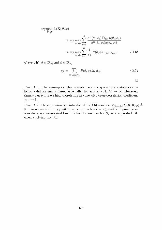
arg maxθ,φ

lc(X;θ,φ)

≈ arg maxθ,φ

d∑i=1

aH(θi, φi) Rxx a(θi, φi)

aH(θi, φi)a(θi, φi)

≈ arg maxθ,φ

K∑k=1

1

χkP (θ, φ) |(θ,φ)∈Sk , (D.6)

where with θ ∈ D∆θand φ ∈ D∆φ

χk =∑

(θ,φ)∈SkP (θ, φ) ∆θ∆φ. (D.7)

Remark 1. The assumption that signals have low spatial correlation can befound valid for many cases, especially, for arrays with M → ∞. However,signals can still have high correlation in time with cross-correlation coe�cientγi,i′ → 1.

Remark 2. The approximation introduced in (D.6) results to ∀(θ,φ)/∈S lc(X;θ,φ) ,0. The normalization χk with respect to each sector Sk makes it possible toconsider the concentrated loss function for each sector Sk as a separate PDFwhen applying the UT.

142

Appendix E

Multivariate AdaptiveRegression Splines (MARS)

The MARS [41] regression model is an extension of piece wise linear regressionmodels. MARS uses a set of splines as basis functions, these splines in turn havethe input variables of the model as their parameters. MARS is an attractiveregression technique due to the fact that it is capable of representing nonlinearrelationships between input and output variables through the multiplicationof basis functions. MARS is also a non-parametric regression model, thereforeit is capable of deriving the relationship between input and output variablespurely based on the data and requires no presumptions.

The MARS model relies on basis functions known as hinge functions. Hingefunctions take the form

h(k, z) =

max(0, k − z)

or

max(0, z − k)

(E.1)

where

max(a, b) =

{a if a > bb if a ≤ b , (E.2)

and k is known as a knot. The set C = {max(0, k− z), max(0, z− k)} is calleda re�ected pair.

Let zi ∈ RI be a vector containing the observations of the I input variablesbelonging to the set I for a given training data observation. Let O be the totalnumber of training data observations and O be the set containing all theobserved values for the input variable during training. The set of candidatebasis functions H for a given MARS model can be built using all the possible

143

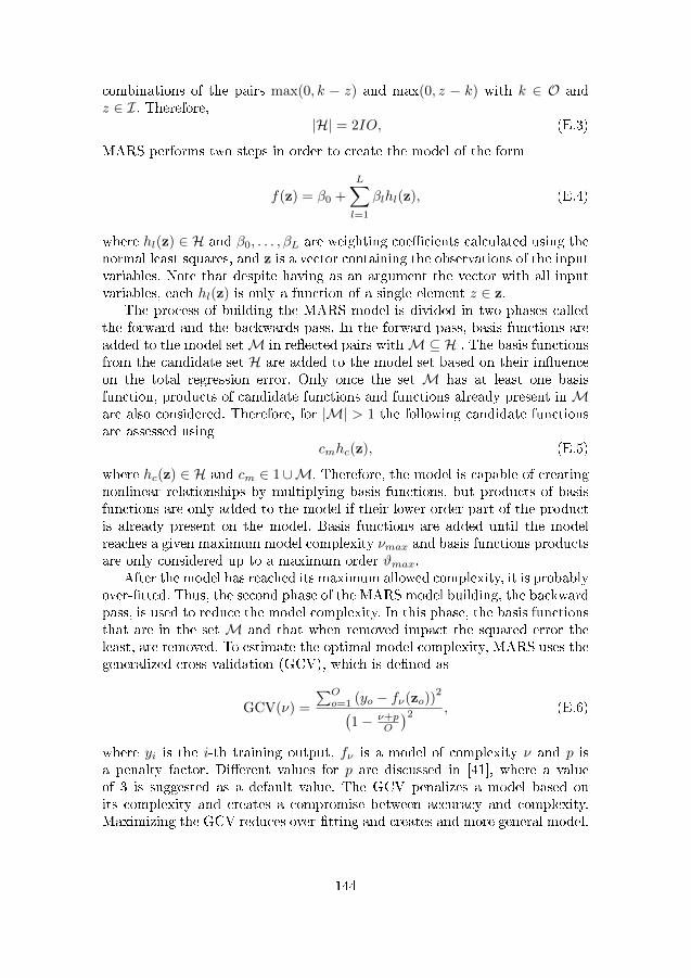
combinations of the pairs max(0, k − z) and max(0, z − k) with k ∈ O andz ∈ I. Therefore,

|H| = 2IO, (E.3)

MARS performs two steps in order to create the model of the form

f(z) = β0 +

L∑l=1

βlhl(z), (E.4)

where hl(z) ∈ H and β0, . . . , βL are weighting coe�cients calculated using thenormal least squares, and z is a vector containing the observations of the inputvariables. Note that despite having as an argument the vector with all inputvariables, each hl(z) is only a function of a single element z ∈ z.

The process of building the MARS model is divided in two phases calledthe forward and the backwards pass. In the forward pass, basis functions areadded to the model setM in re�ected pairs withM⊆ H . The basis functionsfrom the candidate set H are added to the model set based on their in�uenceon the total regression error. Only once the set M has at least one basisfunction, products of candidate functions and functions already present inMare also considered. Therefore, for |M| > 1 the following candidate functionsare assessed using

cmhc(z), (E.5)

where hc(z) ∈ H and cm ∈ 1∪M. Therefore, the model is capable of creatingnonlinear relationships by multiplying basis functions, but products of basisfunctions are only added to the model if their lower order part of the productis already present on the model. Basis functions are added until the modelreaches a given maximum model complexity νmax and basis functions productsare only considered up to a maximum order ϑmax.

After the model has reached its maximum allowed complexity, it is probablyover-�tted. Thus, the second phase of the MARS model building, the backwardpass, is used to reduce the model complexity. In this phase, the basis functionsthat are in the set M and that when removed impact the squared error theleast, are removed. To estimate the optimal model complexity, MARS uses thegeneralized cross-validation (GCV), which is de�ned as

GCV(ν) =

∑Oo=1 (yo − fν(zo))

2(1− ν+p

O

)2 , (E.6)

where yi is the i-th training output, fν is a model of complexity ν and p isa penalty factor. Di�erent values for p are discussed in [41], where a valueof 3 is suggested as a default value. The GCV penalizes a model based onits complexity and creates a compromise between accuracy and complexity.Maximizing the GCV reduces over-�tting and creates and more general model.

144

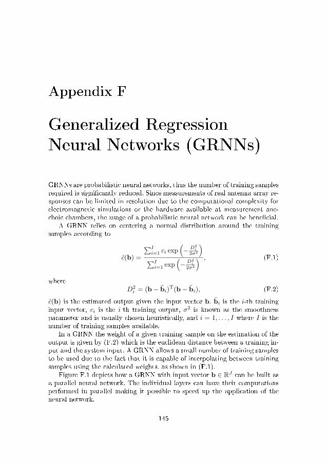
Appendix F

Generalized RegressionNeural Networks (GRNNs)

GRNNs are probabilistic neural networks, thus the number of training samplesrequired is signi�cantly reduced. Since measurements of real antenna array re-sponses can be limited in resolution due to the computational complexity forelectromagnetic simulations or the hardware available at measurement ane-choic chambers, the usage of a probabilistic neural network can be bene�cial.

A GRNN relies on centering a normal distribution around the trainingsamples according to

c(b) =

∑Ii=1 ci exp

(− D2

i

2σ2

)∑Ii=1 exp

(− D2

i

2σ2

) , (F.1)

whereD2i = (b− bi)

T(b− bi), (F.2)

c(b) is the estimated output given the input vector b, bi is the i-th traininginput vector, ci is the i-th training output, σ2 is known as the smoothnessparameter and is usually chosen heuristically, and i = 1, . . . , I where I is thenumber of training samples available.

In a GRNN the weight of a given training sample on the estimation of theoutput is given by (F.2) which is the euclidean distance between a training in-put and the system input. A GRNN allows a small number of training samplesto be used due to the fact that it is capable of interpolating between trainingsamples using the calculated weights, as shown in (F.1).

Figure F.1 depicts how a GRNN with input vector b ∈ RJ can be built asa parallel neural network. The individual layers can have their computationsperformed in parallel making it possible to speed up the application of theneural network.

145

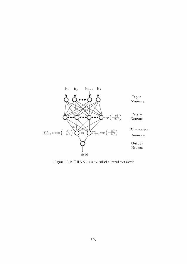
b1 b2 bJbJ−1

Input

Paternexp

(− D2

i2σ2

)

a1

aI∑Ii=1 ai exp

(− D2

i2σ2

) ∑Ii=1 exp

(− D2

i2σ2

) Summation

Output

a(b)

Neurons

Neurons

Neurons

Neuron

Figure F.1: GRNN as a parallel neural network

146

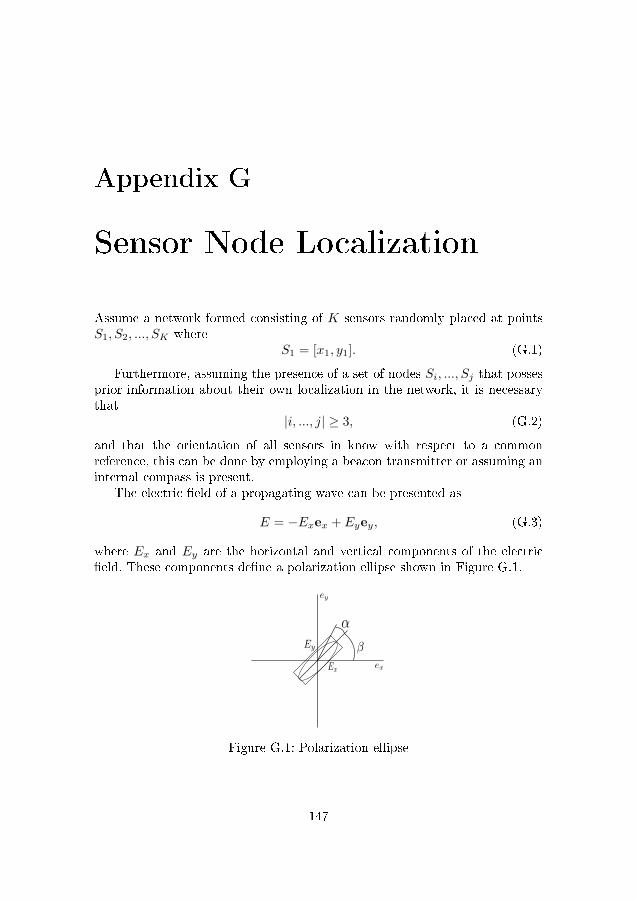
Appendix G

Sensor Node Localization

Assume a network formed consisting of K sensors randomly placed at pointsS1, S2, ..., SK where

S1 = [x1, y1]. (G.1)

Furthermore, assuming the presence of a set of nodes Si, ..., Sj that possesprior information about their own localization in the network, it is necessarythat

|i, ..., j| ≥ 3, (G.2)

and that the orientation of all sensors in know with respect to a commonreference, this can be done by employing a beacon transmitter or assuming aninternal compass is present.

The electric �eld of a propagating wave can be presented as

E = −Exex + Eyey, (G.3)

where Ex and Ey are the horizontal and vertical components of the electric�eld. These components de�ne a polarization ellipse shown in Figure G.1.

Figure G.1: Polarization ellipse

147

Note that the electric �eld components can be written now in terms of theelectric angles α and β as

Ex = E cos(γ) (G.4)

Ey = E sin(γ)ejη (G.5)

where

cos(2γ) = cos(2α) cos(2β) (G.6)

tan(η) = tan(2α) csc(2β). (G.7)

Considering a wavefront impinging over a crossed dipole with componentsparallel to the x− and y − axis of the polarization ellipse the output at suchdipoles will be proportional to the components Ex and Ey respectively and bewritten as

E = (−Ex)ex + (Ey cos(θ))ey

= − cos(γ)ex + sin(γ) cos(θ)ejηey (G.8)

where θ is the angle of arrival of the received wave with respect to the x−axis.The received signal can now be expressed in matrix as

X = us + N (G.9)

where X ∈ C2×N is the matrix containing the measured outputs at each ofthe dipoles, N is the number of measured snapshots, s ∈ C1×N is the vectorcontain the original transmitted signal transmitted, N ∈ C2×N is the matrixcontaining the Additive White Gaussian noise present at sampling and thevector u ∈ C2×1 is de�ned as

u =

[− cos(γ)

sin(γ) cos(θ)ejη

]. (G.10)

This localization approach consists of analysing the ratio between the out-puts of the crossed dipole in order to estimate the direction of arrival of thereceived signal. Given the ratio

r =− cos(γ)

sin(γ) cos(θ)ejη, (G.11)

the angle θ can be obtained by

θ = cos−1

( − cos(γ)

r sin(γ)ejη

). (G.12)

One way to estimate the ratios is to simply average a large number ofsamples from both antennas in order to reduce the e�ects of the noise andobtain the ratio between the powers. It is important to highlight at this point

148

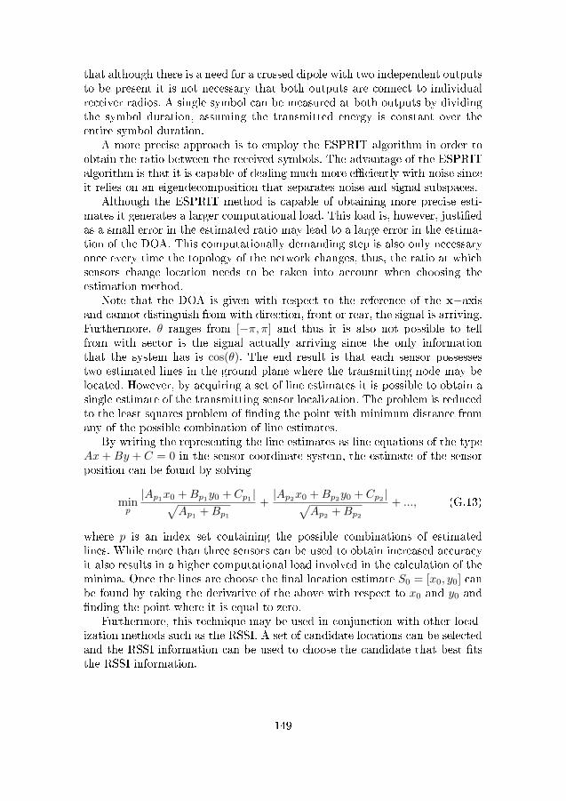
that although there is a need for a crossed dipole with two independent outputsto be present it is not necessary that both outputs are connect to individualreceiver radios. A single symbol can be measured at both outputs by dividingthe symbol duration, assuming the transmitted energy is constant over theentire symbol duration.

A more precise approach is to employ the ESPRIT algorithm in order toobtain the ratio between the received symbols. The advantage of the ESPRITalgorithm is that it is capable of dealing much more e�ciently with noise sinceit relies on an eigendecomposition that separates noise and signal subspaces.

Although the ESPRIT method is capable of obtaining more precise esti-mates it generates a larger computational load. This load is, however, justi�edas a small error in the estimated ratio may lead to a large error in the estima-tion of the DOA. This computationally demanding step is also only necessaryonce every time the topology of the network changes, thus, the ratio at whichsensors change location needs to be taken into account when choosing theestimation method.

Note that the DOA is given with respect to the reference of the x−axisand cannot distinguish from with direction, front or rear, the signal is arriving.Furthermore, θ ranges from [−π, π] and thus it is also not possible to tellfrom with sector is the signal actually arriving since the only informationthat the system has is cos(θ). The end result is that each sensor possessestwo estimated lines in the ground plane where the transmitting node may belocated. However, by acquiring a set of line estimates it is possible to obtain asingle estimate of the transmitting sensor localization. The problem is reducedto the least squares problem of �nding the point with minimum distance fromany of the possible combination of line estimates.

By writing the representing the line estimates as line equations of the typeAx+By + C = 0 in the sensor coordinate system, the estimate of the sensorposition can be found by solving

minp

|Ap1x0 +Bp1y0 + Cp1 |√Ap1

+Bp1

+|Ap2x0 +Bp2y0 + Cp2 |√

Ap2+Bp2

+ ..., (G.13)

where p is an index set containing the possible combinations of estimatedlines. While more than three sensors can be used to obtain increased accuracyit also results in a higher computational load involved in the calculation of theminima. Once the lines are choose the �nal location estimate S0 = [x0, y0] canbe found by taking the derivative of the above with respect to x0 and y0 and�nding the point where it is equal to zero.

Furthermore, this technique may be used in conjunction with other local-ization methods such as the RSSI. A set of candidate locations can be selectedand the RSSI information can be used to choose the candidate that best �tsthe RSSI information.

149

Appendix H

TRIAD Algorithm

The TRIAD [8, 9] algorithm allowed the development of early satellite navi-gation systems and still represents the state of practice for space and aircraftinstrument based attitude estimation. It involves only two linear independentreference vectors and their respective measured directions.

By de�ning two linearly independent reference vectors

~R1 = [x~R1, y~R1

, z~R1]T ,

~R2 = [x~R2, y~R2

, z~R2]T , (H.1)

and their respective measured direction vectors

~r1 = [x~r1 , y~r1 , z~r1 ]T ,

~r2 = [x~r2 , y~r2 , z~r2 ]T . (H.2)

The TRIAD algorithm tries to �nd the rotation matrix W that satis�es

~ri = W ~Ri, (H.3)

where WTW = I and det(W) = ±1, i.e W is a orthogonal matrix and

preserves the magnitude of any vector ~Ri it operates on. Since ~R1 and ~R2 arelinearly independent vectors, a linear independent vector orthogonal to bothcan by obtained by

~R3 = ~R1 × ~R2, (H.4)

where × is the vector cross product operation, the same can be done for ~r1

and ~r2

~r3 = ~r1 × ~r2. (H.5)

Since a rotation applied to ~R1 and ~R2 would also rotate ~R3, a linear systemcan be written as

[~r1, ~r2, ~r3] = R[~R1, ~R2, ~R3], (H.6)

151

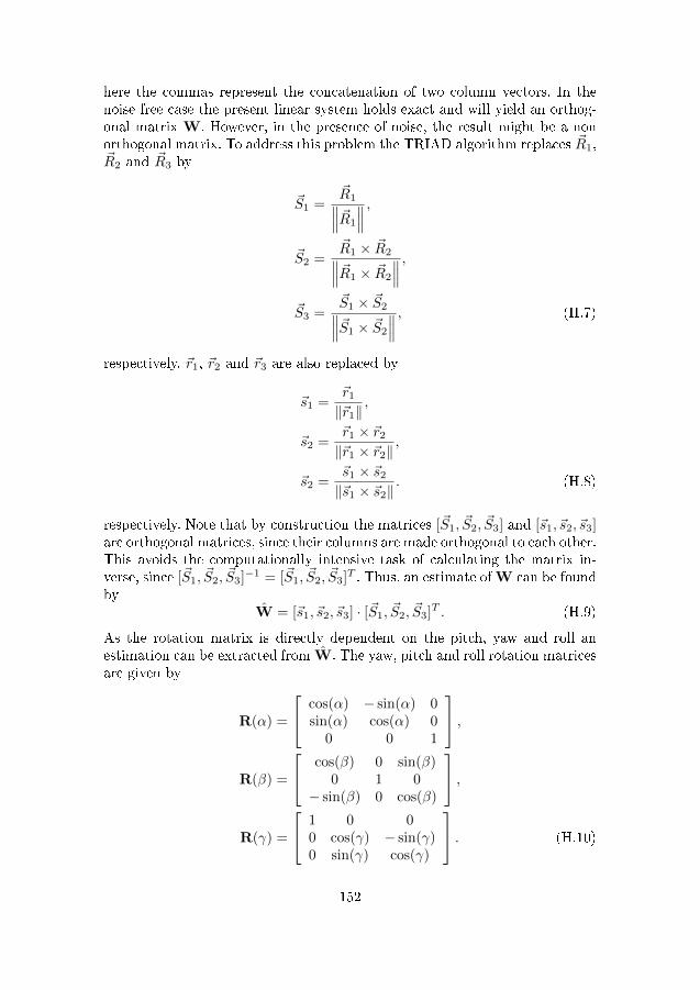
here the commas represent the concatenation of two column vectors. In thenoise free case the present linear system holds exact and will yield an orthog-onal matrix W. However, in the presence of noise, the result might be a nonorthogonal matrix. To address this problem the TRIAD algorithm replaces ~R1,~R2 and ~R3 by

~S1 =~R1∥∥∥~R1

∥∥∥ ,~S2 =

~R1 × ~R2∥∥∥~R1 × ~R2

∥∥∥ ,~S3 =

~S1 × ~S2∥∥∥~S1 × ~S2

∥∥∥ , (H.7)

respectively. ~r1, ~r2 and ~r3 are also replaced by

~s1 =~r1

‖~r1‖,

~s2 =~r1 × ~r2

‖~r1 × ~r2‖,

~s2 =~s1 × ~s2

‖~s1 × ~s2‖. (H.8)

respectively. Note that by construction the matrices [~S1, ~S2, ~S3] and [~s1, ~s2, ~s3]are orthogonal matrices, since their columns are made orthogonal to each other.This avoids the computationally intensive task of calculating the matrix in-verse, since [~S1, ~S2, ~S3]−1 = [~S1, ~S2, ~S3]T . Thus, an estimate of W can be foundby

W = [~s1, ~s2, ~s3] · [~S1, ~S2, ~S3]T . (H.9)

As the rotation matrix is directly dependent on the pitch, yaw and roll anestimation can be extracted from W. The yaw, pitch and roll rotation matricesare given by

R(α) =

cos(α) − sin(α) 0sin(α) cos(α) 0

0 0 1

,R(β) =

cos(β) 0 sin(β)0 1 0

− sin(β) 0 cos(β)

,R(γ) =

1 0 00 cos(γ) − sin(γ)0 sin(γ) cos(γ)

. (H.10)

152

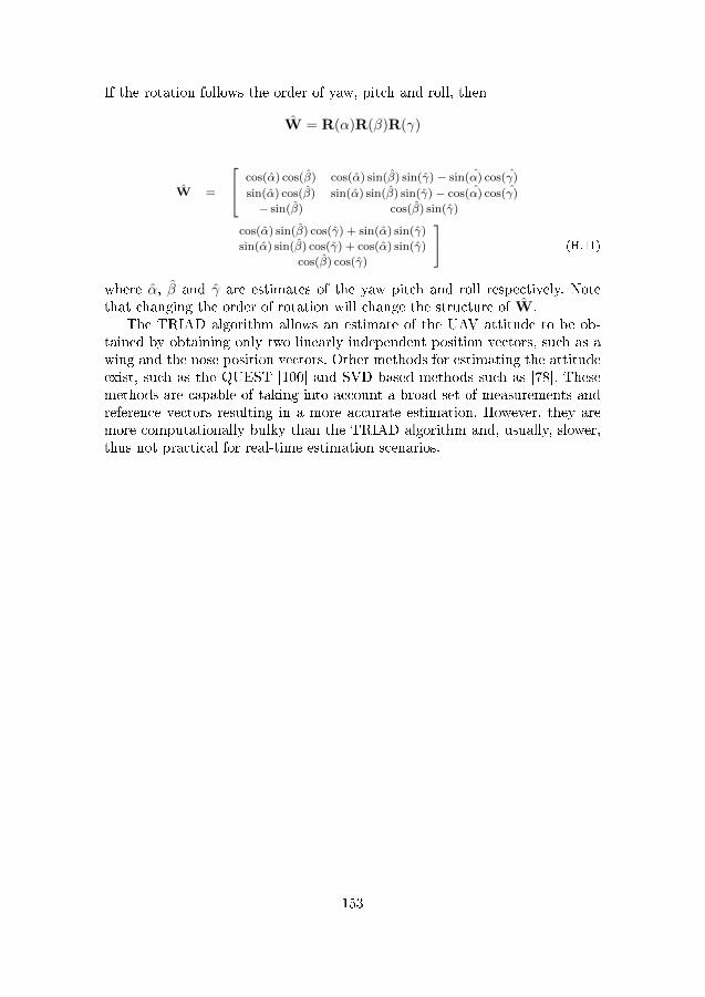
If the rotation follows the order of yaw, pitch and roll, then

W = R(α)R(β)R(γ)

W =

cos(α) cos(β) cos(α) sin(β) sin(γ)− sin(α) cos(γ)

sin(α) cos(β) sin(α) sin(β) sin(γ)− cos(α) cos(γ)

− sin(β) cos(β) sin(γ)

cos(α) sin(β) cos(γ) + sin(α) sin(γ)

sin(α) sin(β) cos(γ) + cos(α) sin(γ)

cos(β) cos(γ)

(H.11)

where α, β and γ are estimates of the yaw pitch and roll respectively. Notethat changing the order of rotation will change the structure of W.

The TRIAD algorithm allows an estimate of the UAV attitude to be ob-tained by obtaining only two linearly independent position vectors, such as awing and the nose position vectors. Other methods for estimating the attitudeexist, such as the QUEST [100] and SVD based methods such as [78]. Thesemethods are capable of taking into account a broad set of measurements andreference vectors resulting in a more accurate estimation. However, they aremore computationally bulky than the TRIAD algorithm and, usually, slower,thus not practical for real-time estimation scenarios.

153