Water Quality Monitoring Guide - State of Oregon: State of Oregon

AN ABSTRACT OF THE THESIS OF
Lihan Huang for the degree of Doctor of Philosophy in Food Science and Technology
presented on June 11, 1997. Title: Application of Membrane Filtration to Recover Solids
from Protein Solutions
Signature redacted for privacy.
Abstract approved:1
Water and waste water accounting was conducted in a shore-based surimi
processing plant. A process flow diagram of the plant was developed and sources of
waste water generation were identified. Waste water samples were collected, analyzed,
and characterized. The gutting and first dewatering operations were two major sources
of the solid wastes (COD, BOD5, and TS), contributing to 60% of total solid wastes. For
every 1 kg of fish processed into frozen surimi, approximately 5.7 L of waste water was
generated. To process 132 x iO3 kg of fish, total waste water generated was 750 m3 per
day, of which 63% (473 m3) was generated in the washing-dewatering processes.
Ohmic heating was used to coagulate fish proteins and partially purify proteolytic
enzymes in surimi wash water prior to membrane filtration. At temperatures above 60°C,
more than 80% and 90% of protein and TSS, respectively, were removed. Between 30
and 60°C, the proteolytic enzyme activity increased linearly with heating temperature.
Denaturation caused a substantial loss of enzyme activity at temperatures above 60°C.
A laboratory scale plate-and-frame crossflow membrane filtration unit was used
to recover myofibrillar proteins from surimi wash water. Four different microfiltration
membranes were used in the study. It was hypothesized that the development of

membrane fouling was a dynamic process of two distinctive stages. Experimental results
showed that the initial membrane fouling process could be modeled by the standard pore
blocking law, and the development of fouling continued with a continuous process of cake
formation. A new concentration-dependent power law cake resistance model was
proposed and verified. The filtration resistance of the cake layer increased with the feed
concentration and was found one order in magnitude higher than the initial dominating
pore blocking resistance.
Finite element analysis was used to simulate the concentration polarization in
ultrafiltration of protein solutions. Protein concentration on the membrane surface and
the mass transfer coefficient were accurately predicted. This simulation method may
provide a useful tool in engineering analysis and design of a membrane filtration process.
©Copyright by Lihan Huang
June 11, 1997
All Rights Reserved

APPLICATION OF MEMBRANE FILTRATION TO RECOVER SOLIDS
FROM PROTEIN SOLUTIONS
By
Lihan Huang
A THESIS
Submitted to
Oregon State University
in partial fulfilment of the requirements for the
degree of
Doctor of Philosophy
Completed June 11, 1997
Commencement June 1998

Doctor of Philosophy thesis of Lihan Huang presented on June 11, 1997
APPROVED:
Signature redacted for privacy.
Major Professor, representing Food Science
Signature redacted for privacy.
of Department of Food Science and Technology
Signature redacted for privacy.
Dean of Graduatei'chool
echnology
I understand that my thesis will become part of the permanent collection of the Oregon
State University libraries. My signature below authorizes release of my thesis to any
reader upon request.
Signature redacted for privacy.
Lihan Huang, Author

ACKNOWLEDGMENTS
I would like to express my thanks to Dr. Michael T. Morrissey, my major
professor, for his encouragement, expert judgement, constructive advice, and consistent
support throughout this research project. My sincere thanks also are directed to the other
committee members, Dr. Jae W. Park, Dr. Edward Kolbe, and Dr. Joe McGuire, for their
professional advice, classroom instruction, and helpful assistance during this study, and
to Dr. Bart A. Thielges, for serving as Graduate School Representative.
Special thanks are extended to Nancy Chamberlain and Lewis Richardson, and all
other graduate students and staff in the OSU Seafood Laboratory, for their help and
encouragement throughout the study; and to National Oceanic and Atmospheric
Administration (NOAA) and the Mamie Markham Endowment Award of the Mark
Hatfield Marine Science Center, Oregon State University, for providing research funds and
financial assistance. Without their support, completion of this research would not have
been possible.
I want to express special thanks to my mother, Ms. Ruiping Zheng, for her
enormous love, for providing me with excellent educational opportunities, and for her
constant encouragement and prayers.
Last but never the least, I want to express my deepest appreciation to my dear
wife, Ying, for her love, emotional and spiritual support throughout the course of my
doctoral study at Oregon State University; and to my daughter, Meghan, for her love and
understanding why Dad has always been so busy. It is to them I dedicate this thesis.
To my wife,
Ying
and to my daughter,
Meghan

TABLE OF CONTENTS
PageINTRODUCTION 1
1.1 Issues of Waste Water from the Surimi Industry 1
1.2 Research objectives 3
LITERATURE REVIEW 4
2.1 Waste water from surimi processing industry 4
2.1 .1 Surimi manufacturing process 4
2.1.2 Waste water generation 8
2.2 Technologies for waste water treatment and product recovery 11
2.2.1 Chemical methods 12
2.2.2 Biological methods 17
2.2.2.1 Aerobic process 17
2.2.2.2 Anaerobic process 19
2.2.3 Physical methods 21
2.2.3.1 Dissolved air flotation 21
2.2.3.2 Heat coagulation 23
2.2.3.3 Electrocoagulation 27
2.2.3.4 Centrifugation 27
2.2.3.5 Membrane filtration 31
2.3 Waste water treatment: reality and perspectives 41

TABLE OF CONTENTS (Continued)
Page3. MEMBRANE FOULING: THEORY AND HYPOTHESIS 45
3.1 Membranes: the Basics 45
3.2 Membrane filtration systems: modules and configurations 48
3.2.1 Dead-end filtration or crossflow filtration 48
3.2.2 Modules 50
3.2.3 Membrane configurations 54
3.3 Permeate flux decline: concentration polarization and membrane fouling 57
3.3.1 Concentration polarization 57
3.3.2 Membrane fouling 58
3.4 Mathematical modeling 60
3.4.1 Empirical and semi-empirical models 60
3.4.1.1 Thin film model 60
3.4.1.2 Resistance-in-series model 65
3.4.1.3 Pore blocking model 66
3.4.1.4 Hypothesis 70
3.4.2 Fundamental models 73
3.4.2.1 Velocity profiles in the membrane flow channel . . . 73
3.4.2.2 Mass transfer in the membrane flow channel 79
3.5 Numerical simulation by finite element methods 80

TABLE OF CONTENTS (Continued)Page
4. MATERIALS AND METHODS 87
4.1 Characterization of waste water generation in the surimi industry 87
4.1.1 Process flow diagram development 87
4.1.2 Audit of water consumption and waste water generation 90
4.1.2.1 Water audit 90
4.1.2.2 Waste water audit 95
4.1.3 Chemical analysis 96
4.2 Treatment of surimi wash water by ohmic heating 97
4.2.1 Ohmic heating device 97
4.2.2 Calibration of the device and determination of electrical
conductivity 99
4.2.3 Sample preparation 100
4.2.4 Coagulation of fish proteins by ohmic heating 100
4.2.5 Chemical analysis 100
4.2.6 Enzyme assay 101
4.3 Microfiltration of surimi wash water 102
4.3.1 Membrane filtration unit 102
4.3.2 Preparation of samples 104
4.3.3 Membranes 104
4.3.4 Characterization of membranes 104
4.3.5 Filtration process 105
TABLE OF CONTENTS (Continued)Page
4.3.5 Filtration process 105
4.4 Finite element analysis of concentration polarization during
ultrafiltration of bovine serum albumin 106
4.4.1 Membrane filtration unit 106
4.4.2 Finite element analysis of concentration polarization
during ultrafiltration 109
4.4.3 Finite element analysis 112
5. RESULTS AND DISCUSSION 114
5.1 Characterization of waste water generation in the surimi industry . . . 114
5.1.1 Process flow diagram 114
5.1.1.1 Subsystem 1 - raw material treatment 114
5.1.1.2 Subsystem 2 - surimi processing 118
5.1.2 Water and waste water audit 119
5.1.2.1 Subsystem 1 119
5.1.2.2 Subsystem 2 122
5.2 Treatment of surimi wash water by ohmic heating 133
5.3 Microfiltration of surimi wash water 143
5.3.1 Effect of membranes on permeate flux and rejection
coefficient 143
5.3.2 Mechanisms of membrane fouling 152

TABLE OF CONTENTS (Continued)Page
5.3.2.1 Pore blocking model 152
5.3.2.2 Cake layer formation 160
5.4 Finite element analysis of concentration polarization during
ultrafiltration BSA 165
5.4.1 Finite element mesh generation 165
5.4.2 Effect of permeate flux on the velocity profiles within the
membrane flow channel 167
5.4.3 Prediction of concentration polarization 172
CONCLUSIONS 182
6.1 Audit of water consumption and waste water generation 182
6.2 Ohmic heating of surimi wash water 182
6.3 Microfiltration of surimi wash water 183
6.4 Finite element analysis of ultrafiltration of diluted BSA solutions . . . 185
6.5 Summary and recommendations for future research 186
NOMENCLATURES 188
REFERENCES 191
LIST OF FIGURES
Figure PageSurimi processing consists of two major stages 6
Washing and dewatering operations in surimi manufacturing 7
Waste water effluents from a multi-purpose seafood processing plant. 9
Chemical structures of synthetic and natural polymeric coagulants 13
Activated sludge treatment of waste water in a maj or waste watertreatment plant 18
A six-phase sequencing batch reactor for treatment of waste waterfrom a meat processing plant 20
An anaerobic process for treatment of waste water from a clamprocessing plant 22
Two types of centrifuges: sedimentation centrifuges and centrifugal filters 28
A decanter centrifuge can be used to recover suspended solids fromthe waste water 30
Recovering whey protein from the waste water of cheese manufacturing . . 34
Phenomenon of osmosis and reverse osmosis 46
Dead-end filtration and crossflow filtration 51
Four commercially available membrane modules. 53
Membrane filtration configurations 55
Schematic diagram of a two-stage series/parallel batch crossflow filtrationsystem 56
Concentration profile in the thin film theory 61
Schematic diagram of pore blocking model 68
Fouling may occur on the surface and in the matrix of membrane 72
Ultrafiltration flow channel with one membrane wall 74

LIST OF FIGURES (Continued)
Figure PageImplicit finite difference grid 82
A generic two-dimentional triangular element 85
The plant could be treated as a big system with interactions with theenvironment outside the boundary 88
The big system may be divided into two subsystems that interac with eachother through an intermediate product, fish mince 89
Each subsystem can contain different numbers of units operations 91
Schematic diagram of a ultrasonic flow meter 92
Time distribution in on-off control of batch operation in Subsystem 2 . . . 94
Ohmic heating device for treatment of surimi waste water 98
A plate-and-frame crossflow membrane filtration unit with a dataacquisition system. 103
Top section of a radial crossflow filter. 107
Bottom section of a radial crossflow filter 108
A radial crossflow ultrafiltration unit with a computer-assiteddata collection system 110
Flow of materials and sources of waste water. 115
Unit operations in Subsystem 1. 116
Unit operations in Subsystem 2. 117
Relationship between temperature and time during ohmic heating of surimiwash water. 134
Electrical conductivity increased linearly with temperature 135
Residual solids concentration decreased with temperature.. 137
Percent reduction of solids increased with temperature. 138

LIST OF FIGURES (Continued)
Figure PageSDS-PAGE of ohmically treated surimi wash water samples. 140
Specific activity of proteolytic enzymes increased upon heating (<60°C)and decreased dramatically at T> <60°C. 142
Changes in permeate flux as a function of filtration time for fourdifferent types of microfiltration membranes. 145
The accumulated permeate volume increased rapidly at the first fewminutes and then increased slowly with time. 146
Dependence of initial flux on feed concentration. 151
SDS-PAGE of surimi wash water samples before and after microfiltration 153
Linear relationship between 1/V and lit at the initial stage of filtration. . 154
Linear relationship between the slopes of the linear region of Fig. 45and the initial flux. 155
Dependence of initial flux on feed concentration. 156
B1 increased exponentially with the permeate concentration. 158
Pore diameter at the end point of pore blocking decreased linearly withfeed concentration. 159
Linear relationship between Ln(V-V) and Ln(t-t) during the continuousdevelopment of the cake layer. 161
The slopes in Fig. 50 increased linearly with the feed concentration. . 162
The intercepts in Fig. 50 decreased linearly with cc. 163
Development of filtration resistance as a function of time.. 164
Finite element mesh generation in the normalized fluid flow channel. 166
The profile of velocity component u in the flow channel at R=0.5. 168
The profiles of velocity component v at the cross section of R=0 5 169

LIST OF FIGURES (Continued)
Figure PageProfile of velocity component u as a function of Z and radius. 170
Profile of velocity component v as a function of Z and radius. 171
Profile of velocity component v as a function of Z and radius. 174
Concentration profile in the membrane flow channel as a function of bothhorizontal and vertical positions.. 176
Development of concentration polarization along the radius direction. 177
Effect of effective diffusion coefficient on the thickness of theconcentration boundary layer. 178
Linear relationship between the calculated boundary layer thicknes anddiffusion coefficient. 179
Mesh generation for D = 7.0 x 10h1 m2/s.. 181

LIST OF TABLES
Table PageDemand charges for industrial waste water treatment in the City of Albany,Oregon 10
Effectiveness of Chitosan in protein recovery 15
3 . Effectiveness of DAF process on pollutant removal in the waste water . . . 24
Proximate composition of cheese whey 33
Effectiveness of UF and RO in treatment of red meat abattoir effluents . . 36
Changes of components in wash water of mackerel meat by ultrafiltration 37
Effectiveness of ultrafiltration (MWCO 50,000) in recovering solids from
blue crab steam cooker effluent 40
Costs of microfiltration systems 42
Differences in reverse osmosis, ultrafiltration, and microfiltration 49
Flow rates and characteristics of waste water generated in Subsystem 1 . . 120
Averaged solid waste flow in the waste water generated in Subsystem 1 . 121
Number of units in washing-dewatering operations in Subsystem 2 123
Time distribution in washing-dewatering operations in Subsystem 2 124
Water consumption in a single washing and rinsing operation 126
Waste water flow rate in dewatering and rinsing operations 127
Characteristics of waste water released in dewatering and rinsing operations 128
Average solid waste generated in dewatering and rinsing operations 129

LIST OF TABLES (Continued)
Table PageCharacteristics of waste water and solid waste flow fromfinal screw press 130
Summary of waste generation in Subsystem 2 132
Coefficients for Eq. 75 for predicting the relationship between residual
concentration and heating temperature 139
Characteristics of microfiltration membranes 144
Concentrations of solids in raw wash water samples and permeates 148
Apparent rejection coefficients during micro filtration of surimi wash
water using different membranes 149
Statistical analysis of effect of membrane materials and pore sizes on steadystateflux and apparent rejection coefficients (ra) during microfiltrationof surimi wash water 150
Input data for the finie element analysis 173
Comparisons of concentrations predicted by finite element analysis andcalculated from Eq. 1 175

APPLICATION OF MEMBRANE FILTRATION TO RECOVER SOLIDSFROM PROTEIN SOLUTIONS
1. INTRODUCTION
1.1 Issues of Waste Water from the Surimi Industry
Surimi is a Japanese term for washed and dewatered fish mince that is widely used
in manufacturing kamoboko or seafood analogs (Lee, 1984). Since it was introduced to
North America about 15-20 years ago, the surimi manufacturing industry has experienced
a steady growth. According to Park (1997), the U.S. annual production of frozen pollock
surimi was 180-190,000 metric tons in the past three years.
Commercial production of surimi involves extensive use of water in various
processing procedures. Apart from the conventional use of water in handling raw
materials (handling, heading, gutting, and washing operations), large volumes of water are
used to remove sarcoplasmic proteins and other unnecessary compounds in the fish flesh
and to concentrate myofibrillar proteins by means of repeated washing and dewatering
until a tasteless and odorless product is obtained. Quality of surimi is highly dependent
on the washing operations.
As a consequence of extensive washing, a large volume of waste water is
generated from the downstream dewatering operations. Not only the soluble proteins are
removed from the fish mince, but also some insoluble myofibrillar proteins, are also lost
in the water. According to Pacheco-Aguilar et al. (1989), 40-50% of the minced fish
solids are lost in the washing and dewatering processes.
Depending on the location of the processing plants, there are different ways of
2
disposing of the waste water. At-sea surimi processing vessels discharge waste water
directly to the open sea where organic wastes are readily dispersed. Although there is
little concern of pollution caused by the disposal of surimi waste water on the high seas,
there is an interest in reclaiming reusable water from the waste streams.
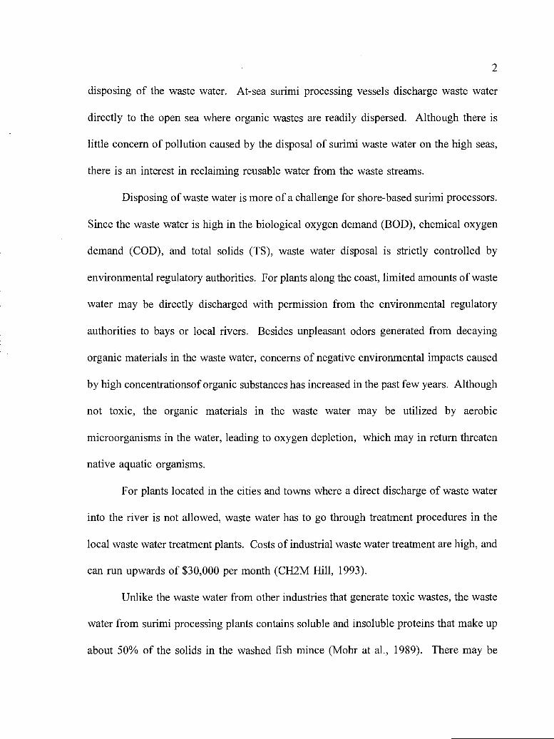
Disposing of waste water is more of a challenge for shore-based surimi processors.
Since the waste water is high in the biological oxygen demand (BOD), chemical oxygen
demand (COD), and total solids (TS), waste water disposal is strictly controlled by
environmental regulatory authorities. For plants along the coast, limited amounts of waste
water may be directly discharged with permission from the environmental regulatory
authorities to bays or local rivers. Besides unpleasant odors generated from decaying
organic materials in the waste water, concerns of negative environmental impacts caused
by high concentrationsof organic substances has increased in the past few years. Although
not toxic, the organic materials in the waste water may be utilized by aerobic
microorganisms in the water, leading to oxygen depletion, which may in return threaten
native aquatic organisms.
For plants located in the cities and towns where a direct discharge of waste water
into the river is not allowed, waste water has to go through treatment procedures in the
local waste water treatment plants. Costs of industrial waste water treatment are high, and
can run upwards of $30,000 per month (CH2M Hill, 1993).
Unlike the waste water from other industries that generate toxic wastes, the waste
water from surimi processing plants contains soluble and insoluble proteins that make up
about 50% of the solids in the washed fish mince (Mobr at al., 1989). There may be
3
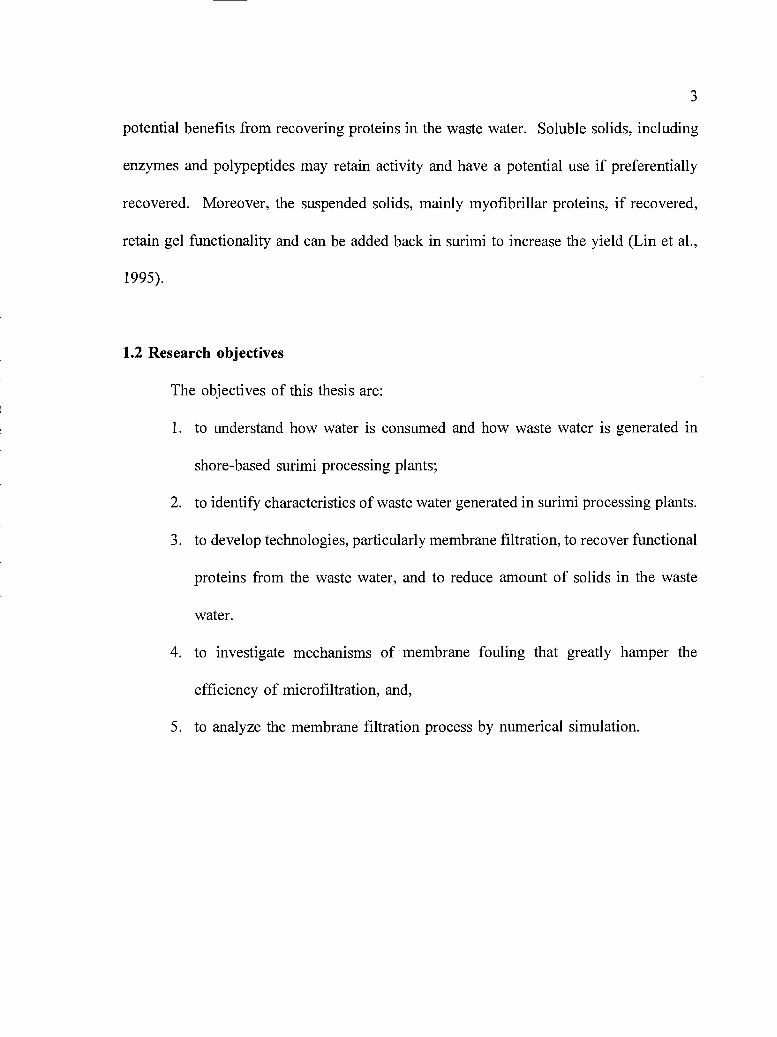
potential benefits from recovering proteins in the waste water. Soluble solids, including
enzymes and polypeptides may retain activity and have a potential use if preferentially
recovered. Moreover, the suspended solids, mainly myofibrillar proteins, if recovered,
retain gel functionality and can be added back in surimi to increase the yield (Lin et al.,
1995).
1.2 Research objectives
The objectives of this thesis are:
to understand how water is consumed and how waste water is generated in
shore-based surimi processing plants;
to identify characteristics of waste water generated in surimi processing plants.
to develop technologies, particularly membrane filtration, to recover functional
proteins from the waste water, and to reduce amount of solids in the waste
water.
to investigate mechanisms of membrane fouling that greatly hamper the
efficiency of microfiltration, and,
to analyze the membrane filtration process by numerical simulation.

2. LITERATURE REVIEW
2.1 Waste water from surimi processing industry
2.1.1 Surimi manufacturing process
The history of surimi can be dated to A.D. 1000 when the Japanese started using
fresh fish mince to make Kamaboko, a Japanese fish sausage (Okada, 1992). Modern
large scale industrial production was not possible until 1959 when the technique for
cryoprotection of surimi was discovered (Matsumoto, 1978). Since then, the world surimi
manufacturing industry has experienced a tremendous growth. The Japanese surimi
operation expanded from small scale shore-based production to larger scale at-sea
operations in the Bering Sea where fishing fleets processed freshly caught Alaska pollock
into frozen surimi. To utilize the abundant resource of Alaska pollock in the U. S., both
at-sea and shore-based surimi operations were established in Alaska. In 1995, 2.85 billion
lbs of Alaska pollock were harvested with a total production of 177.9 thousand mt of
pollock surimi (Johnson, 1996). With the discovery of protease inhibitors, underutilized
fish species such as Pacific whiting were found suitable for making surimi. Since 1992,
four processing plants have been set up in Oregon to manufacture Pacific whiting into
frozen surimi. The annual U. S. harvest and processing of Pacific whiting has increased
from 20,000 mt in 1990 to more than 200,000 mt in 1994 with the majority of the harvest
used for surimi production (Radtke, 1995).
4

5
Surimi processing can be divided into two major stages involving several unit
operations that process raw materials to frozen surimi (Fig. 1). The first stage includes
unit operations (heading, gutting, deboning, and mincing) that prepare fish mince for the
second stage washing. Streams of water are injected to the heading, gutting, and
deboning machines to remove fish fluid and muscles that stick to the machines, and to
provide lubrication for smooth operation. After fish are comminuted into 3-4 mm in
diameter, fish mince is pumped to the second stage.
In the second stage, fish mince is repeatedly washed with chilled water. Washing
and dewatering represent two critical operations to produce high quality surimi. The
major objective of washing and dewatering is to remove soluble sarcoplasmic proteins,
lipids, fish blood, and other water soluble matter in the flesh as well as to concentrate
myofibrillar proteins. Depending on the freshness of raw fish and the desired surimi
quality, water/mince ratio and the number of washing cycles may differ. For at-sea surimi
operations where fresh fish are readily available and water is limited, only one washing
cycle is used, while washing may be repeated 3-5 times for shore-based production (Lee,
1984; 1986; Lin, 1996).
In commercial operations, continuous washing is achieved using several washing
tanks working in sequence (Fig. 2). Each washing is actually a batch operation, in which
fish mince is mixed with a certain amount of chilled water and washed under a mild
mechanical agitation. After washing, mince slurry may be dewatered using a combination
of a rotary screen dehydrator, and a high speed dehydrator, which is essentially a single
screw extruder with a perforated barrel. Washed mince is then pumped to a refiner to

Stage 1
Raw fish
Heading
1
Gutting
Deboning/mincing _I
Fish mince
Waste water
Stage 2
Fish mince
Fresh water IWashing * -
Dewatering- -
Refining
1
Screw pressCryoprotectant
Mixing
Freezing
4Surimi
Fig. 1 Surimi processing consists of two major stages in a typical shore-based processing plant.

First washing cycle
High speed dehydrator
Rotar. Scdehy tor
Fig. 2 Washing and dewatering operations in surimi manufacturing
Second washing cycle
4f
High speed dehydrator

8
remove connective tissues, and squeezed in a screw press to remove excess water. After
mixing with cryoprotectants, surimi is frozen in a plate freezer.
2.1.2 Waste water generation
Surimi manufacturing consumes large volumes of fresh water in its washing
procedures and consequently generates huge amounts of waste water high in BOD5, COD,
and TS. For shore-based surimi production, the overall water/meat ratio may be between
12-24 (Lin,1996). The majority of solid constituents in the waste water are soluble
proteins together with fine meat particles that are lost in the wash water. During washing,
soluble proteins and fine particulate material not retained by rotary screens, which account
for approximately 40-50% of unwashed fish mince, are removed (Lee, 1984; Pacheco-
Aguilar et al., 1989). For a typical multiple-use fish processing plant, the waste levels
(BOD5 and TSS) during processing seasons (April through September) can be 10 times
as high as non-surimi seasons (Fig. 3).
Disposing of waste water poses a real challenge for shore-based surimi processors.
In Oregon, if plants are located in the cities, waste water must go through publicly owned
treatment works (POTW5) to reduce BOD and TS before it can be released into the local
rivers. Charges for each waste water treatment facility are based on the levels of
pollutants, and the total volume of waste water treated (Table 1). The plant represented
in Fig. 3, which generated 50,000 gallons per day of waste water, averaged costs as high
as $30,000 per month (Anonymous, 1994; CH2M Hill, 1993).

10
0.1
BOD ---- TSS
-- --_ '
II
/I
I/
/I
-.-.I
/S.
S.S.
S.
I 2 3 4 5 6 7 8 9 10 11 12
Month
Fig. 3 Waste water effluents from a multi-purpose seafood processing plant (Anonymous, 1994)
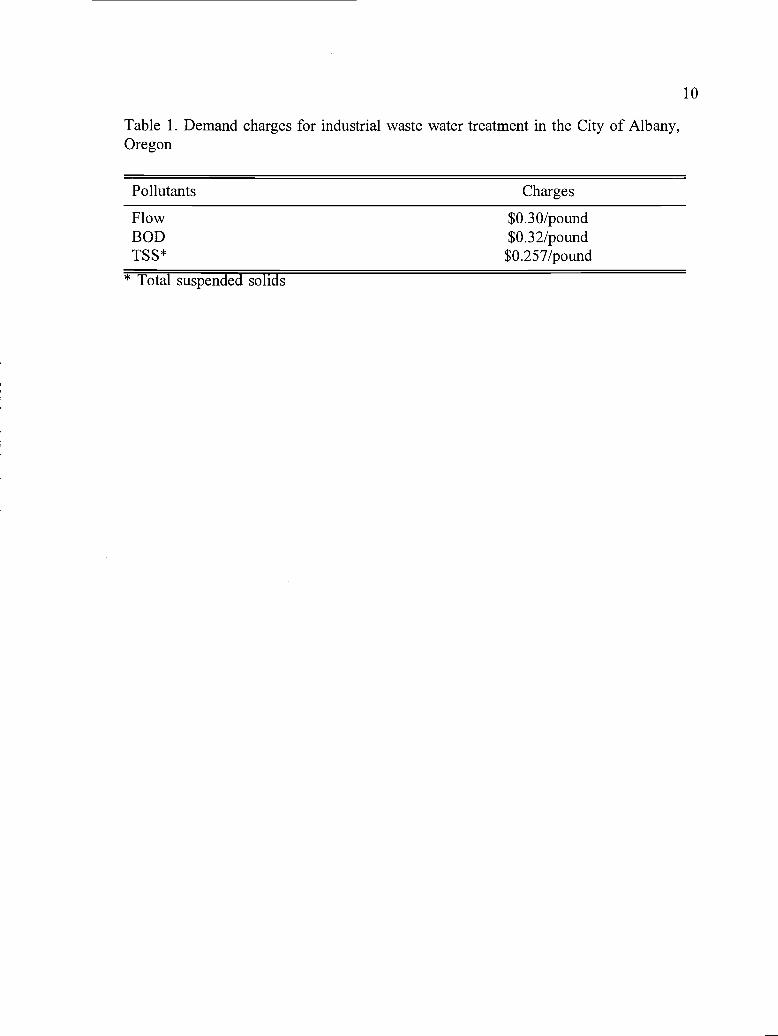
Table 1. Demand charges for industrial waste water treatment in the City of Albany,Oregon
Pollutants Charges
Flow $0.30/poundBOD $0.32/poundTSS* $0.257/pound
* Total suspended solids
10

11
Limited direct discharge of waste water into local rivers and bays is allowable with
permission of environmental regulatory authorities. Since waste water is high in organic
loads, direct discharge can cause potential negative environmental impacts, threatening
aquatic organisms in the water. The waste water effluent has to rapidly mix with the river
current and the pollutants are quickly diluted to a level not harmful to the aquatic life.
If direct discharge is not permitted, waste water has to be hauled away by trucks for
further treatment. Waste water disposal seafood processing has been monitored and
regulated by the environmental regulatory agencies since the 1960's (USEPA, 1967).
Concerns of water shortage, stringent environmental regulations, and the rising costs of
water disposal have caused increasing anxieties among surimi manufacturers.
2.2 Technologies for waste water treatment and product recovery
Generally, the objective of waste water treatment is to clean it up by removing
organic or inorganic solids. If the effluent contains valuable solids that are worth
recovering, waste water treatment is actually a product recovery process. Waste water can
be treated by chemical, biological, and physical methods. Chemical methods involve the
application of chemical agents to coagulate soluble and insoluble materials from the waste
water. Biological methods utilize natural occurring microorganisms to digest the organic
materials. Upon separation of the microbiological cells from the treated waste water, the
organic load in the effluent is significantly reduced. Physical methods use screens, sand
bed filters and, more recently, membrane filters, and other mechanical actions to remove
the solids. Usually, a combination of these methods may be used to achieve effective
12
removal of waste materials in the waste water. The effectiveness of solids removal, costs
of chemicals, and costs of equipment and maintenance are major factors to consider when
selecting a waste water treatment facility.
2.2.1 Chemical methods
Adjusting the pH of the waste water to the isoelectric point of the proteins is the
simplest approach for pretreating waste water. As the pH approaches the isoelectric point,
due to the lack of the electrostatic repulsion between the protein particles, they tend to
aggregate, grow in size and, finally, precipitate. The sedimented proteins can be easily
separated from the waste water (Cheftel et al., 1985).
Soluble ferric and aluminum salts, and their polymeric forms (such as
polyaluminum hydrochlorides), are the most commonly used inorganic coagulants (Lind,
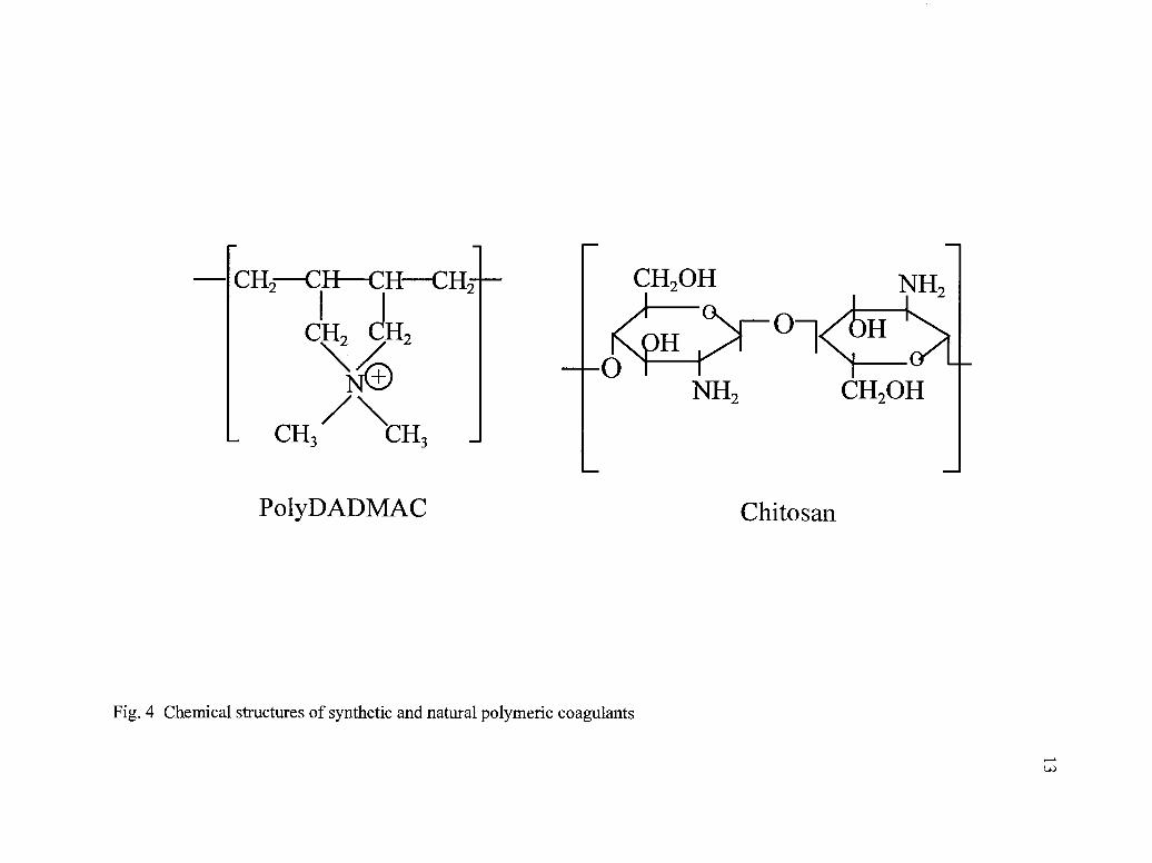
1995). High charge density synthetic polymers (polyelectrolytes), such as polyacrylamide,
po1yDADMAC (dimethyl diallyl diammomiumchloride), and EPIXDMA
(epichorohydrin/dimethyl amine), are widely used in place of aluminum- and iron-based
coagulants (Kasper and Reichenberger, 1983; Lind, 1995). Although these polymeric
coagulants are highly efficient (1O ppm), less expensive, and suitable for a wider range
of pollutants they are, basically, polymeric chains containing large amounts of amine
groups (Fig. 4) that are potentially toxic to human and animals and are not biodegradable.
Acrylamide, the monomer of polyacrylmide, is a highly neurotoxic chemical. Applying
polyacrymide to foods is prohibited. No synthetic chemical coagulants have been
CH2CII CHCH2I I
CH CH2
- CH3/
CH3
Po1yDADMAC
Fig. 4 Chemical structures of synthetic and natural polymeric coagulants
Chito san
14
approved for food applications. Coagulated proteins may not be suitable for human or
animal consumption, and can only be used for landfill.
Similar to synthetic polyelectrolytes, chitosan, a by-product of seafood processing,
is a naturally occuring polysaccharide containing positively charged amine groups (Fig.
4). Since it carries positive changes at acidic conditions, it can attract and destabilize
negatively charged pollutants in the water. Depending on the nature of the waste water,
effectiveness of chitosan in protein recovery may differ (Table 2). Chitosan is partially
deacetylated chitin, which is a natural polymer found in the shells of shellfish. Since
chitosan is biodegradable and non-toxic in nature, it is an ideal candidate for recovering
protein from the waste water (Bough et al., 1975; Knorr, 1991). However, in comparison
to other synthetic coagulants, a large scale application of chitosan for waste water
treatment is cost prohibitive. In recent years, the increased worldwide demand of chitosan
for cosmetic and pharmaceutical applications has led to soaring prices (>$20/lb) for
chitosan (Ludlow, 1997).
Harrison et al. (1992) conducted a series of tests to treat waste water from blue
crab processing facilities. Concentrated sulfuric acid was used to adjust the pH of the
waste water samples to 2.0, 3.0, 4.0, 5.0, and 6.0, respectively. It was found that a range
between 3.0 to 4.0 seemed to be the optimum pH for solids removal. Reductions in COD,
BOD5, TSS, and protein ranged 12%-37%, 6-30%, 76-93%, and 0-24%, respectively.
Final effluents after acidification still showed high BOD5 (2.03-22.4 g/L) and TSS (0.05-
1.05 gIL), suggesting that acidification alone might not be effective in solids removal.

Table 2 Effectiveness of Chitosan in protein recovery (Knorr, 1991)
15
Protein source Chitosanconcentration
(mg/L) pH
Crude proteincontent of
coagulated solids(% dry solids)
Cheese processing 2.5-15 6.0 78
Fruitcake processing 2 4.5 13-22
Meat processing 5-30 6.0-7.3 4115-40 7.4 32-5 1
Poultry processing 6-30 6.4-6.7 34-68
Crawfish processing 150 6.0 27
Mussel processing 40 4.5 38
Shrimp processing 60-360 5.5-6.0 65

16
Watanabe (1974) used both inorganic and organic to coagulate proteins from
marine processing waste water containing fish blood. Waste water was first heated to
70°C, then coagulated with 200 mg/L Al2(SO4)3, and 10 mg/L of a polymeric coagulant.
After filtration, 65-70% and 75-80% reduction in BOD and COD, respectively, were
achieved.
Rusten et al. (1990) studied the efficiency of using FeCl3 and Al2(SO4)3 to remove
organic matters in dairy and slaughterhouse waste water. It was found that pH affects the
coagulation efficiency, with optimum pH dependent upon the chemical agent and dosage.
After proper adjustment of pH, up to 90% of COD can be reduced by the addition of
0.10-0.15 mg/L FeC13.6H20/mg COD or 0.20 mg/L Al2(SO4)3.18H2O/mg COD.
Johnson and Gallanger (1984) compared the efficiency of ferric sulfate and
chitosan in removing organic substances from the waste water of seafood processing
plants. Effluents of crab, shrimp, and salmon processing were tested with different levels
of ferric salts and chitosan. Up to 99% removal of TSS was observed, with chitosan
being more effective. They concluded that, although effective, treatment of seafood waste
water with both coagulants was not economical for seafood processors.
In the surimi industry, polyacrylamide is used in conjunction with other
technologies such as the dissolved air flotation in wastewater treatment (Ismond, 1997).
Application of polyacrylamide to the waste water causes proteins to flocculate and float
to the surface, improving the efficiency of the dissolved air flotation system. However,
the proteins recovered with the addition of polyacrylamide are not suitable for human or
animal consumption.

17
2.2.2 Biological methods
The solids from the food industry waste water are mostly organic solids, such as
protein, peptides, amino acids, sugar and other carbohydrates, animal and vegetable fats,
that can be readily degraded by microorganisms. Biological treatment is the most
successful method for treating large volumes of domestic and industrial waste water. The
basic principle of a biological treatment is to grow cells of microorganisms, usually
bacteria, in aerobic or anaerobic conditions. In both systems, soluble organic materials
are converted to clusters of biological cells that are settlable and easily separated from the
waste water by sedimentation or other conventional separation methods (Fresenius et al.,
1989). Although very effective in reducing organic loads in the waste water, all the
potentially useful nutritive components such as proteins are completely lost.
2.2.2.1 Aerobic process
The activated sludge method is the most commonly used aerobic method in waste
water treatment (Fig. 5). In Japan, surimi waste water is treated with this method after
a primary treatment (Okada, 1992). With sufficient supply of oxygen to the nutrient rich
waste water, organic carbohydrates (C) and proteins (N) are rapidly consumed by bacteria
and other microorganisms and are converted into CO2 and water soluble inorganics
(NH4). The biomass, called "activated sludge", accumulates in the form of flakes
containing a rich flora of aerobic bacteria, some fungi, and some bacteria-eating protozoa.
After treatment, the majority of the sludge is dewatered and can be used as agricultural
fertilizer. Some of the sludge, containing active bacteria, is recycled back to the treatment

Waste water
Primaiytreatmenttank
O2
Activated sludge tank
Large particles
co2
Sludge
NH4
Biomass
Fig. 5 Activated sludge treatment of waste water in a major waste water treatment plant
NO3+!
Denitrification tank
BiomassN2
Treated waste water(to river)

19
tank and used as a bacteria source. In a waste water treatment plant, usually another
aerobic process is followed to grow lower aerobic priority bacteria. This process takes
place in a trickling filter and is called a nitrification process in which NH4 formed during
the activated sludge treatment tank is converted to NO3. The latter can be further
converted into N2 in an anaerobic process. After the complete treatment, organic matter
and harmful inorganic substances in the waste water are removed. After disinfection, the
treated waste water can be directly discharged to rivers (Fresenius et al., 1989).
In a case study by Mikkelson and Lowery (1992), a six-phase sequencing batch
reactor (SBR) system (Fig. 6) was designed to continuously treat high strength waste
water from a meat processing plant. The system was capable of handling 150,000 gallons
of waste water per day. The BOD5, TSS, and NH3-N in the waste water were reduced
from 1,000 mg/L, 200 mg/L, and 7 mgIL, respectively, to 10 mgIL, 10 mg/L, and 2
mg/L, respectively.
2.2.2.2 Anaerobic process
Seafood industry waste water can be treated with anaerobic treatment methods,
since it contains high concentrations of organic matter suitable for the growth of anaerobic
bacteria. Compared to aerobic treatment processes, however, anaerobic treatment is a
slower process due to the slow growth rate of methanogenic bacteria. But because the
process does not require aeration, it is a more economical process for treatment of waste
water with high solids content (COD > 4000 mg/L), and more suitable for treatment of
small quantities of waste water (Fresenius et al., 1989). The volume of sludge formed

Screen DAF
AerobicDigestor
Drying bed
(For grease removal)
Sludge
SBR E.Q.
Sand filter
"VDisinfection
Stream discharge
Fig. 6 A six-phase sequencing batch reactor for treatment of waste water from a meat processing plant

21
in an anaerobic process is smaller than that generated in an aerobic process, and the
generated methane can be used as an energy source. However, the residence time for an
anaerobic process is longer than that for an aerobic process (Fresenius et aL, 1989).
A pilot study was conducted by Cocci et al. (1991) to treat clam processing waste
water using an anaerobic treatment process (Fig. 7). After initial stabilization, COD,
BOD and SS were reduced from 5874, 2342, and 976 mg/L, respectively, to 54.1, 21.6,
and 9.0 mg/L, respectively. More than 80% of solids removal was achieved for all the
pollutants. The authors concluded that the anaerobic process was well suited for treating
clam processing waste water; no additional chemical supplement was needed, and the
biogas produced was of high quality and could be used as an energy source.
2.2.3 Physical methods
Physical methods are usually used in primary treatment of waste water, and
employ one or more physical principles to separate waste materials from the water phase.
For the seafood processing waste water, fish heads, bones, and undersized fish in the
waste water stream are examples of large matter that is separated by physical methods.
In seafood processing plants, the simplest and the most widely used physical method is
the use of screens to trap and prevent large materials from entering the waste stream.
2.2.3.1 Dissolved air flotation
For smaller materials, such as protein particles and particularly fats and oils,
dissolved air flotation (DAF) can be used. In a DAF process, air bubbles are blown from

Samplepump
Day tank
Raw waste water
, I Timer/controllerIIII
I
Reactorsampleport Hand mixer
-Feed pum
AAAAAAAA
Feed Tank
Insulated cooler
Fig. 7 An anaerobic process for treatment of waste water from a clam processing plant
Recycle
Biogas sampleing port
Biogassto atmosphere
) Effluent
Temperaturecontrol

23
the bottom of the waste water stream, causing the undissolved substances to float to the
surface. As a result, a foamlike layer of solids floats upward and accumulates on the
surface of the waste water stream, and can be easily skimmed off (Fresenius et al., 1989).
To improve the efficiency of DAF, a foam generator is usually installed to introduce large
amount of foams into the waste water stream. Depending on the types of solids in the
waste water, the DAF process can be very effective, particularly for treating fat and oil
containing waste water (Table 3).
Hopkins (1983) investigated the effectiveness of combined chemical coagulation
and DAF operations in treatment of waste water from four poultry processing plants prior
to discharge to the city waste water treatment facility. Chemical coagulating agents were
applied before DAF operations. About 5 0-80% efficiencies of removal were observed for
different solids. Since coagulation increased the sizes of protein particles, making them
more difficult to float, and reduced the foaming ability of the protein, the efficiency of
DAF might have been hampered.
DAF was adopted in a surimi processing plant located in Newport, Oregon.
Polyacrylamide was added to the DAF unit, causing proteins in the waste water to
flocculate. The protein flocci, having a lower density that water, floated to the surface of
the waste water, thus reducing the consumption of compressed air (Ismond, 1997).
2.2.3.2 Heat coagulation
Heat coagulation represents another category of physical treatment that can recover
proteins from the waste water for animal consumption. In a heat coagulation process, heat

Table 3 Effectiveness of DAF process on pollutant removal in the waste water (Fresenius et al., 1989)
Types of wastewater
Raw water water Clarified water Purification effect
Undissolved
substance
mg/L
Ether
solublefat
mgIL
BOD5
mgfL
Undissolved
substance
mg/L
Ether
soluble fat
mg/L
BOD5
mgIL
Undissolved
substance
%
Ether
soluble fat
%
BOD5
%
Edible oil production 230 460 2900 20 25 94 91.3 94.6 96.8
Cosmetics production 15000 5405 24500 1800 485 5880 88.0 91.0 76.0
Slaughterhouse 7428 3110 - 712 97 90.4 96.9
Meat processing 970 1706 1540 97 513 277 90.0 70.0 82.0
Poultry processing 1690 331 1075 275 74 86 83.7 77.6 92.0
Animal carcassutilization
5353 4614 780 775 95.4 83.2
Soy bean processing 1656 - 3000 42 800 97.5 73.4
Tomato processing 172 276 59 168 65.7 39.1
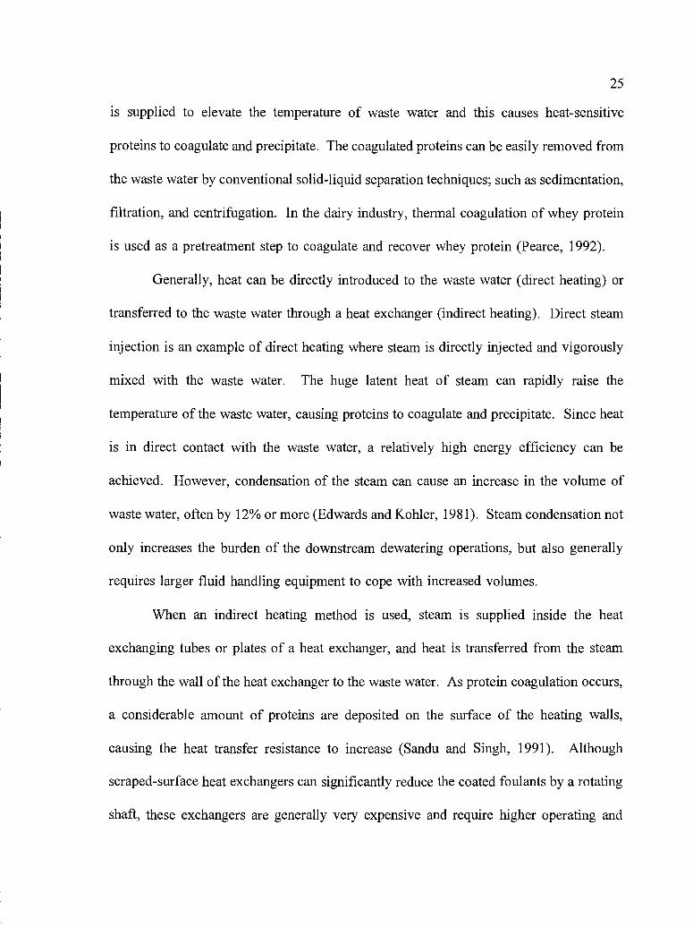
25
is supplied to elevate the temperature of waste water and this causes heat-sensitive
proteins to coagulate and precipitate. The coagulated proteins can be easily removed from
the waste water by conventional solid-liquid separation techniques; such as sedimentation,
filtration, and centrifugation. In the dairy industry, thermal coagulation of whey protein
is used as a pretreatment step to coagulate and recover whey protein (Pearce, 1992).
Generally, heat can be directly introduced to the waste water (direct heating) or
transferred to the waste water through a heat exchanger (indirect heating). Direct steam
injection is an example of direct heating where steam is directly injected and vigorously
mixed with the waste water. The huge latent heat of steam can rapidly raise the
temperature of the waste water, causing proteins to coagulate and precipitate. Since heat
is in direct contact with the waste water, a relatively high energy efficiency can be
achieved. However, condensation of the steam can cause an increase in the volume of
waste water, often by 12% or more (Edwards and Kohier, 1981). Steam condensation not
only increases the burden of the downstream dewatering operations, but also generally
requires larger fluid handling equipment to cope with increased volumes.
When an indirect heating method is used, steam is supplied inside the heat
exchanging tubes or plates of a heat exchanger, and heat is transferred from the steam
through the wall of the heat exchanger to the waste water. As protein coagulation occurs,
a considerable amount of proteins are deposited on the surface of the heating walls,
causing the heat transfer resistance to increase (Sandu and Singh, 1991). Although
scraped-surface heat exchangers can significantly reduce the coated foulants by a rotating
shaft, these exchangers are generally very expensive and require higher operating and

26
maintenance costs.
Ohmic heating is a novel direct heating method, the application of which in the
food industry is gaining momentum. When an alternating electric current is applied to
the material to be heated, due to its electrical resistance, electric energy is directly
converted to heat energy. Ohmic heating is believed to be a more energy efficient
method, and has been developed in the food industry to aseptically process liquid foods
containing particulate suspensions (Stirling, 1987; Biss et al., 1989; de Alwis and Fryer,
1990; Sastry and Palaniappan, 1992). Almost all research efforts have focused on using
ohmic heating to sterilize foods. Huang et al. (1996) investigated ohmic heating in
coagulation of frozen mince wash water. It was found that 33.0%, 59.3%, 33.3%, and
92.1% protein, COD, TS, and TSS, respectively, were removed from the wash water
when the temperature reached 70°C.
Heat treatment to partially coagulate proteins may become necessary when
preferentially extracting water soluble components such as heat stable enzymes from the
waste water. Pacific whiting is a unique fish species that naturally contains active
proteases, particularly cathepsin, in the fish muscle. These enzymes are found to be
responsible for the degradation of functional myofibrillar proteins and gel weakening in
surimi products (An et al., 1994a; An et al., 1994b; An et al., 1995; Seymour et al.,
1994). During washing of the fish mince, some of the proteases are washed out of the fish
muscles. Cathepsin L, one of the major proteases found in Pacific whiting, has a
molecular weight of 28,800 Dalton, and shows a maximum activity at 55°C and pH 5.5.
According to Benjakul et al. (1996), Cathepsin L was found in the surimi waste water

27
collected from a surimi processing plant. The high thermal stability of this enzyme makes
it possible to selectively remove other fish proteins by heat coagulation, and thus partially
purify the protease in the waste water. The removal of other proteins in the waste water
makes it easier for the subsequent purification of the protease. The recovered protease
would have much higher commercial value than fish proteins. According to Huang and
Morrissey (1 997a), a threefold increase in enzyme activity was observed in the ohmically
treated wash water samples.
2.2.3.3 Electrocoagulation
Electrocoagulation is a combined physical and chemical process involving an
alternating or direct current that passes through the waste water to initiate a coagulation
process. Ions released from the electrodes can neutralize the charge-carrying particles in
the waste water, causing them to destablize and coagulate. It is very effective in
removing metal ions, and has also been demonstrated to remove BOD, TSS and oil and
grease from the waste water. Application of electrocoagulation to treat three streams of
waste water from a fish processing plant showed that more than 93% TSS and 35.5-76.9%
COD could be removed (Dalrymple, 1994).
2.2.3.4 Centrifugation
Centrifugation is another conventional method widely used for solid-liquid
separation (Perry et al., 1984). In principle, there are two general types of centrifuges,
sedimentation centrifuges and centrifugal filters (Fig. 8). In a sedimentation centrifuge,

Fluid flow direction
Fluid flow direction
(A) Sendimentation centrifuge
Fluid
mmmm
,.- -., .-..e.--,...wwwwFluid
(B) Centrifugal filter
Fig. 8 Two types of centrifuges: sedimentation centrifuges and centrifugal filters
28
29
a fluid solution containing solid particles is moving under a centrifugal force applied
perpendicular to the moving direction of the fluid. Due to the difference between the
densities of the solid phase and liquid phase, solid particles move along the radius
direction towards the wall of the centrifuge, and then accumulate on the wall, and thus
liquid is separated from the solid phase. If the wall of the centrifuge is a perforated filter,
allowing fluid to pass freely through the wall, then the solid phase will stop and
accumulate on the surface of the filter. This type of filter is a centrifugal filter.
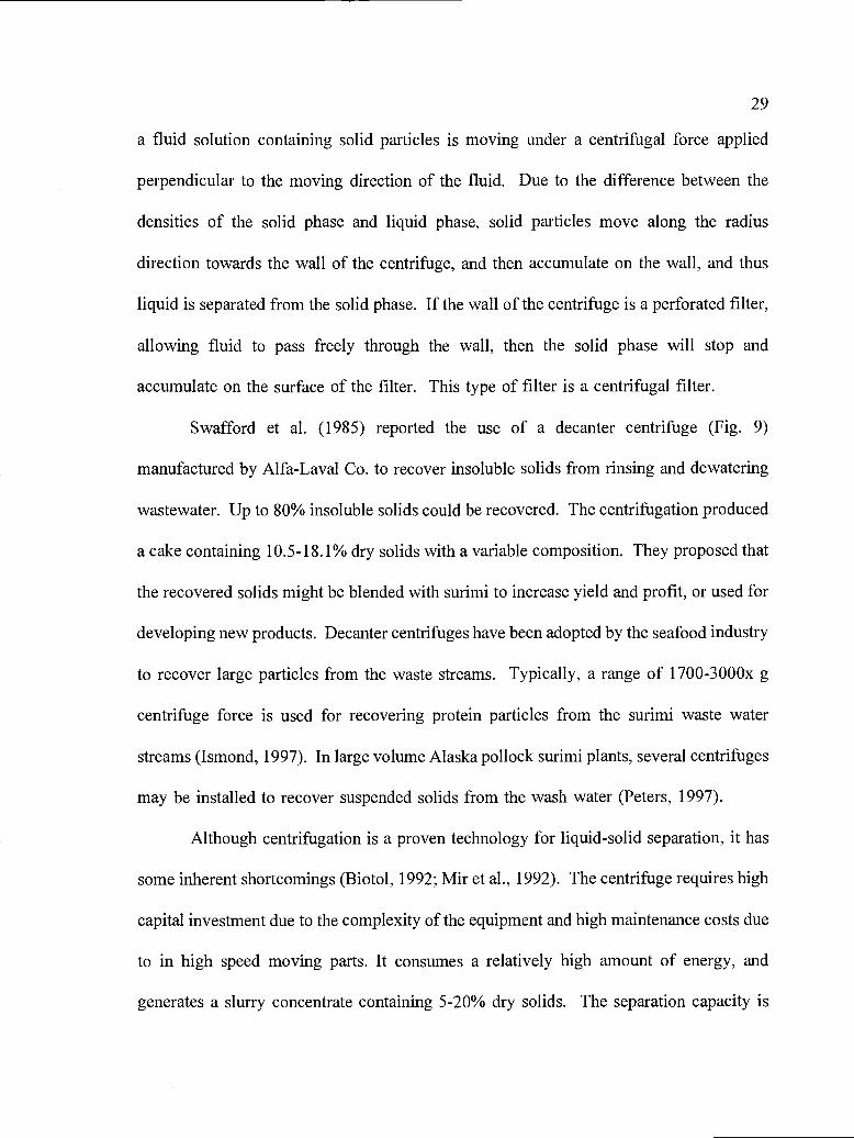
Swafford et al. (1985) reported the use of a decanter centrifuge (Fig. 9)
manufactured by Alfa-Laval Co. to recover insoluble solids from rinsing and dewatering
wastewater. Up to 80% insoluble solids could be recovered. The centrifugation produced
a cake containing 10.5-18.1% dry solids with a variable composition. They proposed that
the recovered solids might be blended with surimi to increase yield and profit, or used for
developing new products. Decanter centrifuges have been adopted by the seafood industry
to recover large particles from the waste streams. Typically, a range of 1700-3000x g
centrifuge force is used for recovering protein particles from the surimi waste water
streams (Ismond, 1997). In large volume Alaska pollock surimi plants, several centrifuges
may be installed to recover suspended solids from the wash water (Peters, 1997).
Although centrifugation is a proven technology for liquid-solid separation, it has
some inherent shortcomings (Biotol, 1992; Mir et al., 1992). The centrifuge requires high
capital investment due to the complexity of the equipment and high maintenance costs due
to in high speed moving parts. It consumes a relatively high amount of energy, and
generates a slurry concentrate containing 5-20% dry solids. The separation capacity is

Fluid
Liquid Solids
Fig. 9 A decanter centrifuge can be used to recover suspended solids from the waste water

31
highly dependent on the particle size and density, which results in an incomplete
separation for the industrial centrifuges.
2.2.3.5 Membrane filtration
Pressure driven crossflow membrane filtration seems to be a natural alternative for
recovering proteins with native functionality from the waste water. When waste water is
pumped across the membrane, water and particles with sizes smaller than the membrane
pores will pass through it, while particles with sizes larger than the membrane pores will
be retained. With the removal of water and smaller particles, solids larger than the
membrane pores will be concentrated.
Membrane filtration employs a positive pressure as a driving force to push the
liquid phase through the membrane pores, without involving a phase change. It is
particularly suitable for recovering and concentrating thermal sensitive components, such
as protein, in the food and biotechnology industry. It has been widely used in the dairy
industry to concentrate milk, to partially remove water from the milk prior to cheese
making, and to recover whey protein and lactose from the waste steams of cheese making
(Cheryan, 1986; Renner and Abd El-Salam, 1991). Using membrane filtration in
concentration and fractionation of milk offers several advantages: 1) reduced overall
energy consumption; 2) increased yield (10-30%) in cheese making; 3) reduced enzyme
(rennet) usage; 4) reduced space requirement due to reduced milk volume; and 5) reduced
environmental pollution due to whey protein recovery.
Recovering whey protein is a successful example of membrane filtration

32
(ultrafiltration, in particular) in the dairy industry (Cheryan, 1986). In cheese
manufacturing, large volumes of cheese whey generated each day are a major problem.
Depending on origination, 8-9 kg of whey can be generated from every 10 kg of milk
(Dziezak, 1990). Due to high concentrations of organic substances in cheese whey (Table
4), very high concentrations of BUD (32-60 gIL) have been observed. According to
Cheryan (1986), about 50% of the approximately 40 billion kg of whey worldwide is
generated in the U.S. Since whey protein shows high gelling, emulsifying functionality,
and potential nutritive values, ultrafiltration (UF) has been applied to concentrate whey
protein by removing water and lactose from the cheese whey (Fig. 10). Permeates from
the ultrafiltration of cheese whey can be further treated with reverse osmosis (RU) to
recover lactose or converted to ethanol by fermentation.
RU is more suitable for recovering smaller molecular weight compounds such as
sugars from the fruit and vegetable industry waste water (Mannapperuma et al. 1993).
A mobile demonstration test unit was launched by the California Institute of Food and
Agricultural Research (CIFAR) to test the applicability of RU in recovering sugars and
reclaiming water from the waste stream of fruit and vegetable processing plants.
Preliminary economic analyses show that benefit/cost ratio of 1.1 and 3.9, respectively,
for a membrane filtration system for recovery of solids concentrates and recycling of
water in peach pitter and tomato peeler operations (Mannapperuma et al., 1993).
In South Africa, treatment of red meat abattoir effluents with membrane filtration
was studied by Cowan et al. (1992). Their research led to a small scale commercial
application (25 m3/d) using full size modules. Polyethersulfone UF membranes with a

Table 4 Proximate composition of cheese whey (Cheryan, 1986)
Total solids 6.60 6.90
Protein (N x 6.38) 0.76 0.85
Ash 0.61 0.53
Fat 0.09 0.36
Carbohydrate (mainly 5.12 5.14lactose)
33
Composition Acid whey Sweet whey

Whey afterfines removal
Evaporator
Balancetank
UF concentrate
Fat separator
25-40% solids
Balancetank
UF plant
UF permeate for utilizationby additional processing
96% solids
Fig. 10 Recovering whey protein from the waste water of cheese manufacturing (Cheryan, 1986)
HTST Pasteurizer Cooler
Balance tank(30mm- 1 hr)
Bagger
55°C
Baggered*- protein
powderPower blenderSpray dryer

35
molecular weight cutoff (MWCO) of 40,000 Dalton were used to directly treat effluents
with preliminary screening (0.5 mm). For a mixed stream of abattoir wastes containing
average COD, TS, conductivity, and soluble phosphate of 6 gIL, 3.5 gIL, 120 mS/rn, and
40 mg/L, respectively, ultrafiltration removed 90% COD and 85% phosphate from the
effluent, and provided a relatively non-fouling feed for reverse osmosis (cellulose acetate)
used to generate reusable water for abattoir use (Table 5). Overall costs for the
membrane filtration system compared favorably with the anaerobic treatment system.
The application of membrane filtration to recover solids from the waste water of
seafood processing has been studied by Japanese scientists. Miyata (1984) used a bench
scale ultrafiltration system to concentrate proteins from the wash water of red muscle fish.
After centrifugation to remove coarse particles, the waste water was pumped to a tubular
filter until a 10/1 volume reduction was achieved. Results (Table 6) showed that about
90% of protein in the feed could be concentrated, and the recovery was independent of
the feed concentration. A more comprehensive study was conducted by Ninomiya et al.
(1985) using ultrafiltration to recover waste soluble proteins in the waste water from
surimi processing plants. Waste water of different fish species was used in their
investigation. An ultrafiltration unit with a MWCO of 20,000 was used to concentrate
the waste water samples containing 0.1-2% protein to 0.4-18% protein. A 90% recovery
was achieved, with proteins having molecular weights higher than 10,000 retained by the
membrane. Microporous membranes were also used to recover solids from the wash
water of fish paste processing (Watanabe et al., 1986 & 1988; Shoji et al., 1988).
Ceramic membranes with pore sizes ranging from 0.05 to 1.5 iim were used in their

Table 5 Effectiveness of UF and RU in treatment of red meat abattoir effluents(Cowan et al. 1992)
UF RU
Feed pressure (kPa) 400 2500
Feed temperature (°C) 20-28 25-30
Rejection %COD 90-93 94-96PO4 85 95Conductivity 25 90-95
Flux (L/m2h) 45 declining to about 20 in 2-3 20-22 with no short-days term decline
36
Feed stream Screened effluent after fat UF filtrateskimming

Table 6 Changes of components in wash water of mackerel meat by ultrafiltration (Miyata, 1984)
Sample Proteins Total solids (B) Protein content Electric Specific gravity(A)
g/100 mLg/ 100 mL (dry base) (A/B) x
100(%)conductivitytc/cm (25°C)
Feed (crude wash) 0.50 0.98 51 4880 1.007
Permeate 0.038 0.53 7.2 4760 1.002
Concentrate 4.8 5.2 92 5480 1.018

38
research. Under high pressure (0.45-0.5 MPa) and low crossflow velocity, a dynamic
membrane was formed within 20 mm due to deposition of soluble proteins on the
membrane surface and inner pores. Almost 100% recovery of protein with molecular
weights> 10,000 Dalton was observed. The thickness of the protein layer deposited on
the membrane surface was about 5 tm, much smaller than that of a ceramic membrane.
This study is an unusual application of microfiltration membranes in recovering soluble
proteins, since the artificially induced dynamic membrane was actually a result of
membrane fouling, which should be avoided in most applications of membrane filtration.
French scientists also conducted research on application of membrane filtration to
recover soluble proteins from the surimi wash water (Jaouen et al., 1989 & 1990; Jaouen
and Quemeneur, 1992). Ultrafiltration membranes with MWCO ranging from 10 - 100
KD were used in their laboratory and pilot experiments. Surimi wash water reconstituted
from freeze-dried sarcoplasmic proteins was used to select suitable ultrafiltration
membranes, and fresh surimi wash water was used in the pilot studies. Results showed
that more than 75% of effluent polluting loads (expressed in BOD5 and COD) could be
reduced with a 100% retention of protein. A clear filtrate, which contained dissolved
amino acids and other lower molecular compounds, was obtained. Permeate fluxes started
from 50 L/m2h at the beginning of filtration and dropped to 10 L/m2h in the end.
Regenerated cellulose membranes performed better than polysulfone membranes due to
their superior hydrophilicity. However, regenerated cellulose membranes are not a good
choice for wastewater treatment since they cannot withstand the harsh chemical conditions
during cleaning and sanitation operations.
39
American scientists started in the 1980s to apply the membrane filtration
technology to seafood processing waste water treatment, and their efforts continue. Chao
et al. (1980; 1983; 1984) applied ultrafiltration to recover the insoluble solids from high
strength crab cooker waste water effluents (Table 7). Batch operations with retentate
recycle were used to achieve a 10:1 volume reduction. Test results show that 60-68%,
60-71%, 17-40%, and 99% of COD, BOD5, TS, and TSS, respectively, were removed
from the waste stream. The permeates were still high in COD and BOD5. They
suggested that a membrane with a lower MWCO should be used, or that a secondary
filtration unit with a lower MWCO (such as 5000 or 10000 Dalton) membrane should be
used to further treat the permeates.
Ultrafiltration to recover proteins from Alaskan pollock surimi wash water was
investigated by Peterson (1990). Plate-and-frame configuration was found superior to
other configurations for filtration of the highly viscous product in an economically
feasible manner Gel strength of recovered protein concentrate was comparable to second
grade surimi Lin et al. (1995) used a microfiltration unit and a spiral-wound polysulfone
(30 KD MWCO) membrane filtration unit to recover solids from surimi wash water.
They found that proteins recovered by microfiltration showed very high gelling
functionality and had a composition comparable with proteins in regular surimi. A 10%
substitution with recovered proteins did not affect the quality of surimi. Solids recovered
by ultrafiltration had considerable dark color and strong odor characteristics, therefore,
were not suitable as a surimi ingredient. An 89-94% reduction in COD was achieved

Table 7. Effectiveness of ultrafiltration (MWCO 50,000) in recovering solids fromblue crab steam cooker effluent (Chao et al. 1980)
40
Pollutants Raw waste (mgIL) Concentrate (mg/L) Permeate(mg/L)
COD 20,000-25,000 67,000-74,000 8,000
BOD5 10,000-14,000 50,000-60,000 4,000
TS 18,000-25,000 52,000-64,000 15,000
TSS 700-1,000 10,000-13,000 10
NH3-N 200-250 240 20
pH 7.0-7.5

41
after UF treatment of Surimi waste water. The UF permeates had a high degree of
clarityand could be potentially recycled (Lin et al., 1995).
Membrane fouling dramatically reduces the efficiency and becomes a major
disadvantage of the membrane filtration process. Usually a large surface area of
membrane and frequent cleaning to remove the fouled layer is needed. Costs of
membranes and systems may vary (Table 8). Polymeric membranes are less expensive
than ceramic and metallic membranes, but they are not as chemical-resistant as ceramic
and metallic membranes. Ceramic membrane filters can have higher fluxes and withstand
strong chemical agents when cleaning, but they are more expensive (Mir et al. 1992).
2.3 Waste water treatment: reality and perspectives
Waste water treatment in the seafood industry is a very complicated issue
raising concerns from environmental regulatory agencies, law makers, the general public,
and seafood processors. The real focus of the issue is to reduce environmental pollution
and also hold down the costs of the waste water treatment.
The Federal Water Pollution Control Act was introduced in 1972 amended in 1977
(also known as "Clean Water Act"), and in 1987 (known as "Water Quality Act") to
regulate waste water disposal in the United States. The Marine Protection, Research and
Sanctuaries Act (MPRSA) was passed in 1972 and amended in 1988 (known as "Ocean
Dumping Ban Act of 1988"). The MPRSA covers discharge into the ocean past the three
mile territorial sea boundary. The Clean Water Act governs discharges into nearshore
waters, rivers, and estuaries; therefore, the Act currently covers any seafood processing
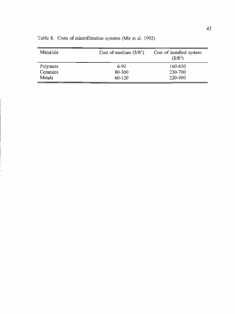
Table 8. Costs of microfiltration systems (Mir et al. 1992)
Polymers 6-90 160-650Ceramics 80-300 230-700Metals 60-120 220-900
42
Materials Cost of medium ($ift2) Cost of installed system($/ft2)

43
effluent discharged directly into these waterways. In 1974, the Safe Drinking Water Act
was passed to prevent ground water contamination. In 1974, USEPA established
limitation guidelines that required seafood processors to employ the Best Available
Technology (BAT) to treat waste water (Forsht, 1974). These guidelines set the standards
for waste water disposal, and are also referred to as BAT standards that should have been
enforced by 1983. However, the BAT standards have been considered by industry as not
achievable due to the high costs of waste water treatment. In 1978, the BAT standards
were reviewed by USEPA and replaced with the "Best Conventional Pollutant Control
Technology (BCT)" standards. The BCT standards are less strict and easier to implement
in the industry. From the governmental standpoint, the success of waste water pollution
control can only be achieved by strictly enforcing rules and regulations for pollution
control and prevention. This may temporarily curtail the economic activities of small
businesses, but it will help develop a more environmentally friendly industry.
The seafood industry must be willing to treat and reduce waste water, and
cooperation with federal and local environmental regulatory agencies is necessary to
develop short-term and long-term waste water reduction and treatment strategies.
Technically, waste water from the seafood or other sectors of the food industry is not
difficult to treat, but costs for the treatment can be high.
It is important for seafood processors to develop environmental awareness among
their employees and to educate them not to waste fresh water (Ismond, 1994). It would
be very helpful for companies to establish a water saving plan. This plan must include
guidelines for fresh water usage and spent water recycling in the places where fresh water

44
is not needed. Any activities leading to water usage savings should be encouraged, and
any activities leading to increased waste water generation discouraged. From the technical
standpoint, to achieve a cost effective and successful waste water treatment, it is necessary
to develop a prioritized plan. There are many sources in a company that generate waste
water, and not all the points produce high levels of waste. There are usually only a few
point sources that generate the waste water high in BUD, COD, TS, and TSS. Waste
water from these points must be separated from the other waste water streams, and to do
so requires a prioritized treatment. The majority of low strength waste water can be
treated with less expensive technologies since not all the treatment methods cost the same.
It is necessary to clearly define goals for solids recovery, as they directly
determine the technology to be employed and the costs for operation and maintenance.
It is not hard to comprehend that a technology adopted to recover solids for human
consumption is more expensive than for animal feeds or landfills. Therefore, a
combination of different technologies for achieving different goals and meeting different
criteria is needed for the most cost effective waste water treatment.
3. MEMBRANE FOULING: THEORY AND HYPOTHESIS
3.1 Membranes: the Basics
Development and application of modern artificial membranes have been closely
related to the phenomenon of osmosis discovered in 1748 by the French scientist Nollet.
A classical experiment can be used to demonstrate the phenomenon of osmosis (Fig. 11),
and the principle of reverse osmosis. In an apparatus shown in Fig. 11-A, two L-shape
tubes are separated by a membrane that is permeable to water but not to solutes. The
solution in the left tube has a higher concentration and therefore possesses a higher
osmotic pressure than the one in the right tube. Due to the difference in osmotic pressure,
water in the right tube will migrate to the left tube. As a result, the solution volume in
the left tube will increase until an equilibrium is reached when the osmotic pressure in
both tubes equals (Fig. 11-B). If an external pressure is applied to the left tube to
overcome the difference in the osmotic pressures, water in the left tube will be forced to
move to the right tube. Consequently, the level of the solution in the right tube rises (Fig.
11-C). This process is called reverse osmosis.
At the early stage of membrane development, scientists and engineers showed a
tremendous interest in the potential applications of membranes. The artificial kidney was
one of the most significant developments that brought hope to many end-stage kidney
patients. During World War II, Kolff and Berk (1944) applied the principle of dialysis
and developed a method that used cellulose film as a membrane to reduce the
concentration of metabolic end products in the blood of a kidney patient. Although
45

(A)
(B)
(C)
C1
Cl
C1
.(C1>C2)
........ _(,
.Membrane
SS
V S
Fig. 11 Phenomenon of osmosis and reverse osmosis
' S
C2
46

47
primitive by today's standards, their experiment led to the development of a new therapy
for thousands of end-stage kidney patients worldwide (Drukker et al. 1983).
Another force driving the development of modern membranes is to perfect a
process to extract fresh water from seawater. This research was of critical importance to
national defense during the cold war when submarines had to cruise under the sea for long
periods without fresh water supplies. In 1953, C. E. Reid, Professor, University of
Florida, initiated studies of seawater desalination by reverse osmosis (Madsen, 1977;
Longsdale, 1983). The real breakthrough, however, took place in the late 1950s at the
University of California, Los Angeles where the first high flux asymmetric cellulose
acetate membrane was developed by Loeb and Sourirajan. Funds from the U.S.
Department of Interior Office of Saline Water supported the research. Since then, new
membrane materials and devices have been developed and commercialized. Membranes
with larger pore sizes for ultrafiltration and microfiltration were also developed.
A membrane is actually a thin sheet of artificial or natural polymeric material with
pores distributed in it. Under a certain pressure, species smaller than the pores can pass
through, while large particles are rejected by the membrane. Pore sizes and pore size
distribution determine the type and performance of a membrane. Reverse osmosis
membranes have pore sizes smaller than 2 nm, usually operating under a very high
pressure (15-80 bar), and they are particularly suitable for rejecting small species such as
ions. Ultrafiltration membranes have pore sizes between 1-100 nm, operating under a
medium range of pressure (1-10 bar). They are suitable for rejecting macromolecules
such as soluble proteins with molecular weights between 300-500,000 Daltons. Based on

48
the ability to reject solutes, ultrafiltration membranes are categorized by their nominal
molecular weight cutoff, or MWCO, which is usually defined as the smallest molecular
weight at which molecules will be rejected by the membrane. Microfiltration membranes
are even larger in pore sizes (0.05-10 tm). Since these membranes have very porous
pores, they are particularly suitable for retaining large particles, such as viruses, bacteria,
and other biological cells. Reverse osmosis, ultrafiltration and microfiltration are all
pressure driven processes, but differ in the ability to reject particles in the solutions (Table
9).
Saudi Arabia seems to have benefited the most from the membrane filtration
technology (particularly reverse osmosis). Many desalination plants have been installed
there, including the world's largest plant (57,000 m3/day) in Saudi Arabia (Muhriji et al.,
1989; Woj cik, 1983). The semiconductor industry is a maj or user of membrane filtration
technology to generate "particle free" or ultrapure water for semiconductor and integrated
circuit processing. The pharmaceutical industry is another big user of membrane filtration
technology in process for concentration, fractionation, clarification, and sterilization of
parenteral drugs (Geol et al., 1992; Mir et al., 1992a).
3.2 Membrane filtration systems: modules and configurations
3.2.1 Dead-end filtration or crossflow filtration
There are two types of membrane filtration: dead-end filtration and crossflow
filtration. In a dead-end filtration process, fluid flows perpendicular to the membrane

Table 9 Differences in reverse osmosis, ultrafiltration, and microfiltration (combined from Mulder, 1990)
Membranestructure
Thickness
Pore size
Driving force
Separatingprinciple
Membranematerials
Main applications
asymmetric or composite
sublayer 150 tm; top layer 1 Jim
0.05-10 pm
pressure: brackish 15-25 barseawater 40-80 bar
solution-difusion
cellulose acetate, aromatic polymide,poly(ether urea)
- desalination of seawater- production of ultrapure water forelectroinc industry
- concentration of food juice andmilk
asymmetric porous
150 jim
1-100 nm
pressure: 1-10 bar
sieving
polymer (polysulfone,polyacrylonitrile)ceramic (zirconium oxide,aluminum oxide)
- concentration of milk andwhey protein
- pharmaceutical industry(concentration of enzymes,antibiotics, pyrogens)
- electropaint recovery
(a)symmetric porous
10-150 jim
<2 nm
pressure: <2 bar
sieving
polymer (polysulfone)ceremic
- analytical applications- sterilization (food,
pharmaceuticals)- ultrapure water(semiconductor)
- cell harvesting andmembrane bioreactor
- plasmapheresis
Reverse osmosis Ultrafiltration Microfiltration

50
surface. Due to a rapid accumulation of solutes on the membrane surface, the permeate
flux declines dramatically (Fig. 12-A). This filtration type is widely used in laboratories
for filtering small volume liquids. It is also used in the pharmaceutical industry for sterile
filtration (Geol et al., 1992).
Crossflow filtration is a major, revolutionary concept in the development of
membrane filtration technology. In crossflow filtration, fluid flows in a direction
tangential to the membrane surface (Fig. 12-B). In addition to the pressure applied
normally to the membrane surface, a shear force is exerted tangentially to the membrane
surface, removing the solutes accumulated on that surface. A steady state filtration can
develop after the shearing force is in equilibrium with the forces that lead to the
accumulation of the solutes on the membrane surface. The permeate flux in crossflow
filtration is much higher than that of dead-end filtration. Crossflow filtration is
predominately used in reverse osmosis, ultrafiltration, and microfiltration.
3.2.2 Modules
Other than inorganic membranes made of ceramic or stainless steel, most
membranes are thin sheets of organic polymers, and are mechanically fragile. For
laboratory purposes, membranes are sold in disks, rectangular sheets, or rolls. For larger
scale operations, membranes are built into customized housings, called modules.
Membrane module designs should be 1) mechanically strong to protect the membrane and
housing; 2) hydrodynamically fit to prevent concentration polarization and membrane
fouling; and 3) inexpensive to fabricate and replace (Bhattacharyya et al., 1992). After

(A)
(B)
::u:::: is::::::'
Fluid flow, shear force
' " ' ' XI
1Permeate
Fluid flow, pressure
I
Permeate
Pressure
I
Fig. 12 Dead-end filtration and crossflow filtration
Time
Cake thickness
Time
Permeate flux
Permeate flux
Cake thickness
51

52
years of development, plate-and-frame, tubular, spiral wound, and hollow fiber modules
are four major membrane modules commercially available.
Plate-and-frame modules (Fig. 13-A) were some of the first modules tested and
commercialized. In a plate-and-frame unit, fluid flows into one end of a thin rectangular
channel and leaves at the other end as a retentate. The permeate flows through the wall
(membrane) of the channel. The packing density of plate-and-frame units is between 100-
400 m2/m3 (Rautenbach and Albrecht, 1989).
Tubular design (Fig. 13-B) is another popular module. In a tubular unit, a narrow
sheet of membrane is rolled into a tube (diameter> 10 mm) and supported by an external
stainless steel, ceramic, or plastic tube (Mulder, 1990). Usually 4-18 tubes are packed
together in a housing. Feed flows into the tube and the liquid permeates through the wall
of the membrane. Due to the large tube diameter, turbulent flows can be pumped into the
membrane tubes. It is a design with the least fouling or concentration polarization
problem. Packing density is usually less than 300 m2/m3.
Hollow fiber design (Fig. 13-C) is the most popular design for reverse osmosis.
A bundle of small membrane tubes having an internal diameter 40-100 tm and an
external diameter of 80-200 pm is molded to a membrane housing. A feed can flow into
the fiber tubes or from outside the tubes. This design has the highest packing density
(<30,000 m2/m3). A hollow fiber module is most suitable for clean feed streams, since
it is a structure most likely to foul.
The spiral wound design is the most widely used module. In this type of module,
two sheets of membrane, sandwiched with a permeate channel spacer and a feed flow

Permeate
Permeate
Fig. 13 Four commercially available membrane modules
Feed
Permeate
(D)
..___. 0 0 ',JjEfI0 ,-°'I
. okY
&YøAAwy&p1WA
kVø
0
4y-
AAAW
AIA!AYAPAYYIYYA
AAWAWAY4YaYAWAW#
WØA
(B) Permeate
54
channel spacer are glued and rolled together around a center tube where the permeate
collects (Fig. 13-D). This design has a moderately high packing density (300-1000
m2/m3), and is suitable for relatively clean feeds with a turbidity <1 NTU. Cleaning a
spiral wound membrane filter is difficult, however.
3.2.3 Membrane configurations
During membrane filtration, membrane modules may be installed in different
configurations. For small fluid quantity operations, batch concentration with retentate
recirculation is most commonly used (Fig. 14-A). Using this configuration, the feed
concentration increases with the removal of the permeate, which increases the tendency
of membrane fouling. The process is an unsteady state operation.
The feed-and-bleed configuration (Fig. 14-B) is used to concentrate solids in the
feed in a steady state operation. Most of the retentate is recycled back to the feed
solution, while a small portion of the retentate is bled off as a product. Because of
retentate recirculation, feed flows at a high velocity to the filter, reducing the tendency
of fouling.
In large scale membrane filtration operations, one stage is usually not sufficient
to obtain a desired retentate concentration or permeate quantity. Many modules can be
connected in a serial or parallel manner with multiple arrays of membrane modules that
are arranged to handle a large volume of fluids (Fig. 15). This type of operation is called
a cascade operation. Depending on characteristics of the feed and desired final
concentration of the retentate, a combination of module arrangement can be used.

A. Batch operation
Feed
B. Feed-and-breed operation
Retentate
Fig. 14 Membrane filtration configurations
Permeate
Retentate breed
Permeate
55
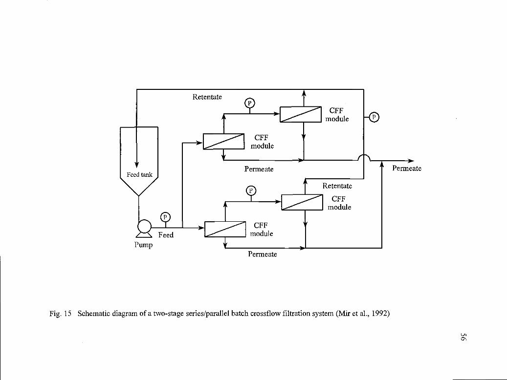
'V
Feed tank
FeedPump
Retentate
CFFmodule
Permeate
9)CFF
module
Permeate
CFFmodule
Retentate
CFFmodule
(ThA Permeate
Fig. 15 Schematic diagram of a two-stage series/parallel batch crossflow filtration system (Mir et al., 1992)

3.3 Permeate flux decline: concentration polarization and membrane fouling
3.3.1 Concentration polarization
Membrane filtration would have gained more applications without the problems
of concentration polarization and membrane fouling. When starting with pure water, the
permeate flux is very high. When solutes are present in a feed solution, a dramatic
permeate flux decline results. In early years of membrane filtration, membranes were
used to remove salts and some macromolecules from water. Permeate flux decline was
found to be related to the buildup of the solutes with a high concentration near the
membrane surface. A high osmotic pressure due to the concentration buildup near the
membrane surface reduces the overall driving force (Eq. 1). Within a certain range, the
permeate flux increases with the pressure. At very high pressures, J becomes
independent of AP, which may attribute to the increased solution concentration, or
consolidation of the membrane. In some severe cases, solids may form an insoluble layer
deposited on the membrane surface. At that point, membrane fouling may have occurred.
(1)
The permeate flux decline caused by concentration polarization is considered
temporary, and can be adjusted or removed by changing the feed concentration. If there
exist no other fouling mechanisms that lead to flux decline, rinsing the membrane unit
with pure water can totally restore the permeability of the membrane.
57
1 List of symbols and their definitions is located in Chapter 7.

58
3.3.2 Membrane fouling
Prolonged filtration of biological molecules may lead to formation of a gel-like
layer that can dramatically reduce the permeate flux. For soluble protein molecules, the
gel or gel-like layer on the membrane surface is considered an extension of the
concentration polarization layer in which the solubility of the solutes reaches the critical
limit (Nilson, 1990). These solutes form a layer of deposits through physicochemical
associations with the membrane surface, and thus irreversibly modifies the membrane
characteristics in terms of both permeate flux and rejection capability. This phenomenon
is called membrane fouling.
Different mechanisms of interactions between solutes and membranes have been
conceptualized. Belfort et al. (1994) stated that several phenomena are responsible for
membrane fouling and they summarized that fouling may be a 5-stage process. During
the very early phase of membrane filtration, the membrane surface is immediately exposed
to the macromolecular solutes in the feed. Adsorption of the macromolecular solutes on
the membrane may occur quickly within the membrane structure and on its surface. The
second stage involves the development of a monolayer adjacent to the membrane surface.
During this stage, the suspended solids slowly deposit on the membrane surface until the
whole surface is completely covered. The interaction between the solutes and the
membrane controls the rate of monolayer development. The third stage continues with
the buildup of multi-sublayers resulting from the interactions between the solutes. The
filtration resistance increases significantly. Increasing the pressure may temporarily
increase the permeate flux, and it also leads to a compression in the deposited layers,

59
which in turn reduces the flux. When the multilayer growth reaches its maximum,
densification of the sublayers may occur. The permeate flux is affected by the
rearrangement of the particles on the membrane surface. This is the fourth stage of
fouling. If the filtration is a batch process, removal of permeate from the feed leads to
increased concentration and viscosity. The bulk solution may become a non-Newtonian
fluid, thus precipitously decreasing the permeate flux (Belfort et al. 1994).
There is a distinct difference between concentration polarization and membrane
fouling. Concentration polarization involves a concentration gradient near the membrane
surface. It may be affected by the hydrodynamic conditions in the membrane filtration
system. The membrane structure and characteristics (pore size and porosity, i.e.,
permeability) are not affected by the concentration buildup on the membrane surface
(Marshall et al., 1993). Membrane fouling, on the other hand, is the consequence of
interaction between the feed solution and the membrane, leading to modified pore
structure and surface characteristics of the membrane.
Multilayer protein adsorption and deposition may play an important role in the
development of membrane fouling (Ingham et al., 1980). A protein layer of 0.5-1.0 tm
deposited on the membrane surface has been reported by Lee and Merson (1975) and
Cheryan and Merin (1980). Compared with the monolayer protein deposition (1 mg/m2),
up to 1 g/m2 of protein deposition can be found in fouled membranes (Nilson, 1990).
Protein deposition on the membrane surface is highly pH dependent. According to Suki
et al. (1984), maximum bovine serum albumin (BSA) deposition was observed at pH
around the isoelectric point (p1) of BSA. In another study, however, the protein
60
deposition was found to decrease with an increase in pH. Matthiasson (1983) used "C-
BSA solution to investigate the mechanism of membrane fouling at various pH using
different membranes. He found that at pH below p1 the positively charged BSA molecules
may enhance the interaction with the negatively charged membrane surface. At alkaline
pH conditions, both protein molecules and membranes (cellulose acetate and polysulfone)
are negatively charged. An electrostatic repulsion exists between the membrane surface
and protein molecules, leading to reduced protein deposition.
3.4 Mathematical modeling
3.4.1 Empirical and semi-empirical models
3.4.1.1 Thin film model
The thin film model first proposed by Brian (1966), is still the most successful
theory in membrane science. Although developed for reverse osmosis, the thin film
model is also applied to ultrafiltration and microfiltration (Blatt et al., 1970; Colton et al.,
1975; van den Berg and Smolders 1988; Zydney and Colton, 1986). The thin film model
was developed based on the concentration polarization theory. It is assumed that there
is a solute concentration gradient developed near the membrane surface (Fig. 16). The
solute is transported to the membrane surface by the permeate flux, leading to a
concentration buildup on the membrane surface. Existence of the concentration gradient
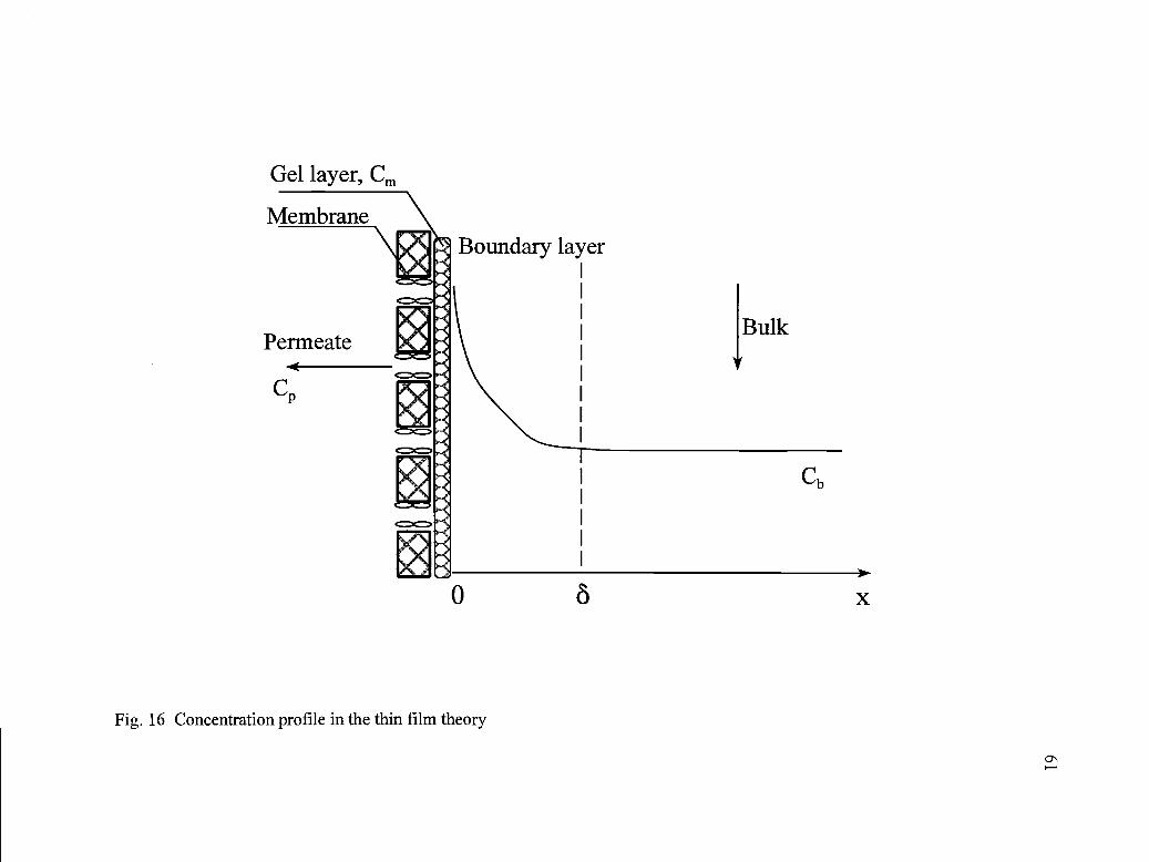
Gel layer, Cm
Membrane
Permeate
Cp
Fig. 16 Concentration profile in the thin film theory
o x

62
causes the solute to transport back to the feed stream. At a steady state, a very thin layer
of concentration gradient develops. Within the boundary, the solute mass transport is
governed by:
JC-D=JC.dx
(2)
The boundary conditions for Eq. 2. are:
x=O, C Cm
x=, C=Cb
After integration of Eq. 2, the permeate flux J can be expressed as a function of
feed concentration Cb, the permeate concentration C, and the solute concentration Cm Ofl
the membrane surface (Eq. 3). The ratio of diffusion coefficient D and the thickness
of the boundary layer is the mass transfer coefficient k. The thin film model can be
rewritten as (Eq. 4).
as r,
Defining the apparent rejection coefficient as ra, and the true rejection coefficient
Ln(Cm - Cp Jo J (3)
Cb-CpJD k
J = k Lfl(C -C) - k Ln(Cb-Cp) (4)

Cr = 1 -a
CbC
r = 1 -Cm
the thin film model can be further written as:
rkLn(
raJ =kLn(
J - 1_ra)
From Eq. 4 or Eq. 6, the mass transfer coefficient k and the solute concentration
Cm on the membrane surface can be experimentally determined. If J is plotted against
Ln(Cb-CP) or Ln(ral(l-ra)), a linear relationship should be observed.
Under the assumption of concentration polarization theory, the property of the
membrane is not altered during membrane filtration. The performance is affected by the
hydrodynamics of the membrane filtration system, and is related to Sherwood, Reynolds
and Schmidt numbers (Mulder, 1990).
Sh = aRe)ScckHSherwood number = Sh = - -D
Reynolds number = Re - Hu (7)
V
Schmidt number = Sc = =D
63
(5)
(6)
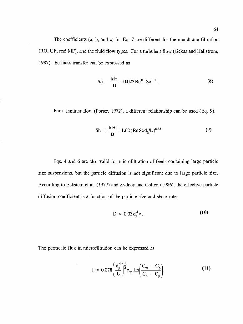
64
The coefficients (a, b, and c) for Eq. 7 are different for the membrane filtration
(RO, UF, and MF), and the fluid flow types. For a turbulent flow (Gekas and Hallstrom,
1987), the mass transfer can be expressed as
Sh = O.O23Re°8Sc°33. (8)D
For a laminar flow (Porter, 1972), a different relationship can be used (Eq. 9).
Sh = kH=1.62(ReScd1JL)°33
D(9)
Eqs. 4 and 6 are also valid for microfiltration of feeds containing large particle
size suspensions, but the particle diffusion is not significant due to large particle size.
According to Eckstein et al. (1977) and Zydney and Colton (1986), the effective particle
diffusion coefficient is a function of the particle size and shear rate:
D = O.O3dy. (10)
The permeate flux in microfiltration can be expressed as
/ 4\1(d Lfl(m -J = O.O78)Cb -

RSCCbV
65
3.4.1.2 Resistance-in-series model
Resistance-in-series model is based on the traditional filtration theory (van den
Berg and Smolders, 1988). In this model, the total filtration resistance is composed of
two parts: the resistance of the clean membrane and the resistance of the cake layer
deposited on the membrane surface. The permeate flux is proportional to the applied
pressure, and can be described by the Darcy's Law (Eq. 12) (Belfort et al., 1996). This
model assumes that there is no interaction between the feed solution and the membrane,
and that the internal structure of the membrane is not modified by the permeate. In a
dead-end filtration process, the cake continues to grow as permeate passes through the
membrane. If all the solutes and particles are rejected and retained by the membrane, the
cake layer resistance is proportional to the thickness of the cake layer (Eq. 13).
Substituting Eq. 13 to Eq. 12, a new model can be derived (Eq. 14). Eq. 14 is commonly
known as the Ruth's law (Suki et al., 1984; Nakao et al., 1986), and is widely used to
model dead-end filtration processes. If t/V is plotted against the accumulated permeate
volume, a straight curve should be observed.
1 dVAm dt IL(Rm + R)
R=RL-C SC C
CmAm

66
During the early stage of crossflow, the development of the cake layer on the
membrane surface also follows Ruth's law (Iritani et al., 1991; Tanaka et al., 1993;
Murase et al., 1995). As crossflow filtration progresses and reaches a steady state, the
interaction between the deposited layer and the feed solution is stabilized. Then t/V in
Eq. 14 becomes independent of the filtrate volume.
3.4.1.3 Pore blocking model
When filtering soluble proteins or suspended protein particles through a membrane
with pore sizes significantly larger than the proteins, some proteins may enter the
membrane matrix and interact with the pore walls of the membrane and accumulate in the
inner pores (Marshall et al., 1991; Bowen, 1993; Kawakatsu et al., 1993). The flow path
of membrane pores may be reduced due to the adsorbed layer of proteins on the pore
walls. The pore blocking model is based on an assumption that the amount of protein
deposited on the pore walls is proportional to the permeate passing through the pores
(Blanpian et al., 1993; Bowen and Gan, 1991; Bowen and Gan, 1992; Bowen and Hall,
1995).
In development of the pore blocking model, a membrane is assumed to have a
uniform thickness and uniformly distributed parallel cylindrical pores. The initial pore
V
Rt+
RCse b (14)
APAm 2Am2 A P

67
has a diameter of d0, and a height of h (Fig. 17). Assuming the protein molecules or
particles form a uniform coating on the inner pores and the porosity of the coating solids
is negligible, then the pore volume decreases proportionally to the total permeate volume:
--Nhd(d) ms
2
att =0,d =d0,V =0,at t = t, d=d, V = V
In Eq. 15, m5 is the amount of solids deposited on the membrane inner walls per
unit volume of the permeate. By integrating both sides of Eq. 15, as shown in Eq. 16,
the total permeate volume can be expressed as a function of pore diameters (Eq. 17).
Nhp (d2 - d2)4m5
d v
f- Nnd(d) = ffdV
(15)
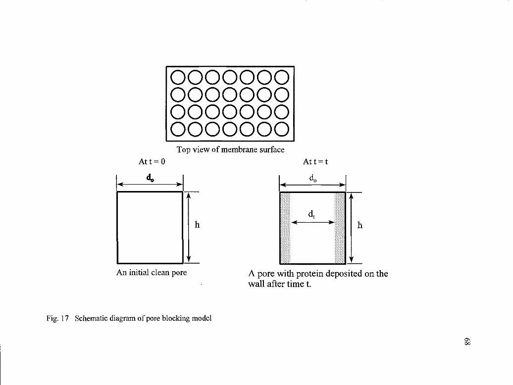
Top view of membrane surface
Att=O Att=t
An initial clean pore
0000000000000000000000000000
h
Fig. 17 Schematic diagram of pore blocking model
d0
h
A pore with protein deposited on thewall after time t.
kd0

69
For membrane filtration under a constant pressure AP without a cake layer
deposited on the surface, the permeate flux is governed by the Hagen-Poisseuille law (Eq.
18):
1 dV_cd4LPNAm dt 128J.Lth
Combining Eq. (17) and Eq. 18, then
Denoting the initial pore volume as
d 2hV- °N.0
(18)
(20)
dY = JA
= J0Am
1-
1-
d2-d2o p dt
V dt.
(19)d
4m2irNhpd0

70
Integrating Eq. 19, the pore blocking model can be obtained (Eq. 21).
1 1 1 m8 _K (21)V JoAmt
If plotting 1/V against l/t, a straight line can be observed if the filtration process
is governed by the pore blocking law. The slope in Eq. 21 is proportional to 11J0, and can
be used to estimate the membrane area.
3.4.1.4 Hypothesis
Eq. 14 is derived from the traditional dead-end filtration process with an
assumption that all the solid particles are completely rejected and retained by the
membrane surface. During microfiltration of a protein solution containing particles with
different particle sizes, particles larger than the membrane pores will be rejected by the
membrane, and smaller particles will penetrate into the inner pores. According to Suki
et al. (1984), the linear relationship tiV and V was observed only in the initial stage of
crossflow filtration, while non-linear relationship was observed in most filtration
processes, suggesting that a different cake formation mechanism may be responsible for
the non-linear relationship between t/V and V.
During the initial stage of microfiltration, the initial permeate flux is much higher
than the steady state flux and declines in a very short period. The high initial permeate
flux can bring more particles into the pores and deposit these within the pores, causing
the pathway to narrow rapidly.

71
In microfiltration of surimi wash water, where fouling may occur both in the inner
pores and on the membrane surface (Fig. 18), the membrane resistance in Eq. 14 is not
that of the clean membrane, but that of the membrane with fouled internal pores. Since
the composition of the surimi wash water is so complex, the rejection of solids cannot be
100%. Both pore narrowing and cake formation may develop depending on the stage of
the filtration process. Assume that the pore blocking is the dominating resistance during
the initial stage, and that cake resistance begins to develop at time t-t, where t is the
reference time point at which fluid flow begins to stabilize. Assuming that the total
filtration resistance R is a nonlinear function of the total volume of permeate (V), it can
be expressed as:
R- 1 (yy)act43
where a is a function of solids concentration, and Iis a constant to be empirically
determined Obviously, the total resistance R is composed both of the resistance of a
membrane with fouled pores, and of the boundary layer near and the cake layer deposited
on the surface.
Substituting Eq. 22 into Eq. 12 and by integration, it can be obtained that
(22)
v-v = ) (t-t). (23)

Deposited layer
Membrane
(B)Flow direction
Bulk feed
0
Deposited layer
Membrane
00
g.Qo0
Ms
0Permeate
Fig. 18 Fouling may occur on the surface and in the matrix of membrane
72
(A) Flow direction

73
Taking logarithms on both sides of Eq. 23 transforms it into a linear relationship
between Ln (V-Vs) and Ln (t-t):
Ln (V -) = a Ln ( APA + a Ln (t -ta) = + a Ln (t -ta) (24)
3.4.2 Fundamental models
3.4.2.1 Velocity profiles in the membrane flow channel
Consider a feed solution containing protein molecules that is pumped into a plate-
and-frame membrane filter (Fig. 19). The filter flow channel is composed of two parallel
walls, with one being a membrane and the other an impermeable wall. The feed is
flowing tangentially across the flow channel with a height of H and length of L. A
coordinate system is chosen with the origin located at the entrance point of the
impermeable wall. The z axis is perpendicular to the channel wall toward the membrane
surface. If 1) the filtration is at a steady state; 2) the fluid is incompressible; 3) the flow
is laminar; 4) the velocity (flux) of the permeate leaving the membrane wall is
independent of position, then the fluid flow within two parallel walls is governed by
Navier-Stokes equations. These equations are expressed as (Berman, 1953):
av vav lap v la2vU- + -- = --- + V + -ax ax päx ax2 2ax2
(25)

z
(0, H)
(0, 0) (L, 0)
Fig. 19 Ultrafiltration flow channel with one membrane wall

75
The boundary conditions for the Navier-Stokes equations are (Kleinstreuer and
Paller, 1983; Ganguly and Bhattacharya, 1994):
u(x,±l) = 0
( =0(29)
v(x,0) = 0
v(x,l) = J.
For a laminar flow, the fluid enters the membrane channel having a parabolic
velocity profile, with an average velocity ü0. According to Berman (1953) and
Kleinestreuer and Paller (1983), a stream function (x, z) exists such that the continuity
equation could be satisfied (Eq. 30).
au v3uu+--= lap---vpax
f'a2u+
la2u (26)ax HA 1ax2 }{22J
au
axlay
+ = 0 (27)ax
zA (28)
H
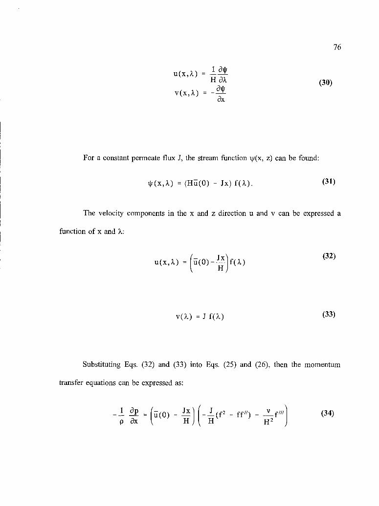
For a constant permeate flux J, the stream function V(x, z) can be found:
iV(x,A) (Hii(0) - Jx) f(A).
The velocity components in the x and z direction u and v can be expressed a
function of x and 7:
u(x,) = ((o)H)
(32)
v(X) = J f(X) (33)
Substituting Eqs. (32) and (33) into Eqs. (25) and (26), then the momentum
transfer equations can be expressed as:
Jx (_J(f2 - ff") -- = (o- H H2pax
lailiu(x,X) = -
v(x,X)ax
(34)
76
(30)
(31)

1 ap v8v_ vhp ax ax H2 ax2
Since ap/a2. in Eq. (35) is only a function of 2, and is independent of x, it is
possible to differentiate Eq. (34) and Eq. (35) with respect to 2. and x, respectively, such
that
a2p0axax
After differentiation with respect to 2, Eq. (34) becomes
Jx\ d J2 - ff") + _f" = 0.Iu(0)--I (H)dxH H2
If Eq. 37 has to be satisfied for all x, then
d(J_(fa - ff") + --f" = 0.H2 ,d H
Defining the Reynolds number in the z direction as
Re =JH (39)
V
77
(35)
(36)
(37)
(38)

78
Integrating Eq. 38, a new equation involving f(X) only can be obtained (Eq. 40):
Re(f'2 - ff") + fl/I = k,
where k is the integration constant.
The boundary conditions for the newly derived Eq. 40 are:
at X = 0, f' = f =0;ar ? = 1, f" = Oand f = 1
Since the permeate flux during membrane filtration is very small, Re is also very
small and is in the range of 0.005 0.05 (Kleinstreuer and Paller, 1983; Bouchard et al.,
1994), then the first term in Eq. 40 become negligible and
f" k. (42)
A perturbation solution to Eq. 40 is possible (Berman, 1953; Singh and Laurence,
1979; Kleinstreuer and Paller, 1983; Bouchard et al., 1994) using Re as a perturbation
parameter, by expanding f(A) and k as a power series (Eqs. 43 and 44).
f(X) = f0C) + f1(A)Re + 12()Re + + f(X)Re + (43)
k = k0 + k1 Re + k2 Re2 + ... k Re + (44)
Substituting Eqs. 43 and 44 into Eq. 40 using the first order perturbation and,
(40)
(41)

79
applying the boundary conditions, u and v can be expressed as a function of x and X
(Kleinstreuer and Paller, 1983).
Re 1
u(x,X)=I(xj)_J(x)'[6X_62+_286+84X5_1O5X4+81X2_32J
H 70 (45)
Rev(x,X) =J(x) 32_2X3 z(_4Xl146_215273_16X2) (46)
70
The term J(x1) in Eqs. (45) and (46) is the average permeate flux in the i-th
segment on the discretized membrane surface.
3.4.2.2 Mass transfer in the membrane flow channel
If the feed solution contains only a single small specie such as BSA with a very
low concentration, then concentration polarization is the main resistance causing the flux
decline. As the feed flows across the membrane surface under a positive pressure, the
solute in the feed solution is convected to the membrane surface by the permeate, causing
the concentration to build up in the vicinity of the membrane surface. The high solute
concentration near the membrane causes the solute to diffuse back to the main stream.
Neglecting the diffusion in the x direction, the steady state convection-diffusion mass
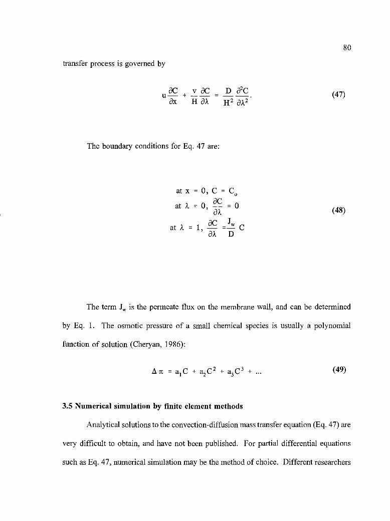
transfer process is governed by
aC vC DCU- + -- =ax HaA H2a2
The boundary conditions for Eq. 47 are:
at x = 0, C = C0
at A = 0, = 0ax
acat A = 1, - =- Cax D
The term J, is the permeate flux on the membrane wall, and can be determined
by Eq. 1. The osmotic pressure of a small chemical species is usually a polynomial
function of solution (Cheryan, 1986):
= a1C + a2C2 + a3C3 + (49)
3.5 Numerical simulation by finite element methods
Analytical solutions to the convection-diffusion mass transfer equation (Eq. 47) are
very difficult to obtain, and have not been published. For partial differential equations
such as Eq. 47, numerical simulation may be the method of choice. Different researchers
80

81
have attempted to solve Eq. 47 numerically by a finite difference method to predict the
concentration profile within the flow channel (Brian, 1965; Singh and Laurence, 1979;
Kleinstrauer and Paller, 1984; Lebrun et al., 1989; Bouchard et al., 1994; Ganguly and
Bhattacharya, 1994). Solutions of the mass transfer equation by finite element methods
have not been cited in the literature.
Solving partial differential equations numerically by finite difference methods
involves subdividing the problem domain into a finite number of grids to achieve a finite
number of solution points, choosing a calculation algorithm, applying the boundary values,
and then calculating the values in the next grid points based on the previous points (Fig.
20). The number of grids and points determines the accuracy of the approximation. Using
the implicit method, Eq. 47 can be transformed into a numerical computation form:
C. C.. C . 2 C..u.. t,31 -v.. tl,j1 1'1 =ii: '1' i,j 11,J1
2Az Az2
The finite element method is a numerical simulation technique that can produce
near-optimal approximate solutions to initial-boundary value engineering problems (Baker
and Pepper, 1991). This approximation method employs subdivision of the problem
domain into a finite number of small regions called finite elements. Applying a weak
statement or a weighted-residual that minimizes the approximate errors combined with the
boundary conditions, a set of algebraic equations can be developed on each finite element,
and then collected to form a global matrix statement. The matrix can be solved using any
linear algebra technique to obtain the variable values in the problem domain (Baker and
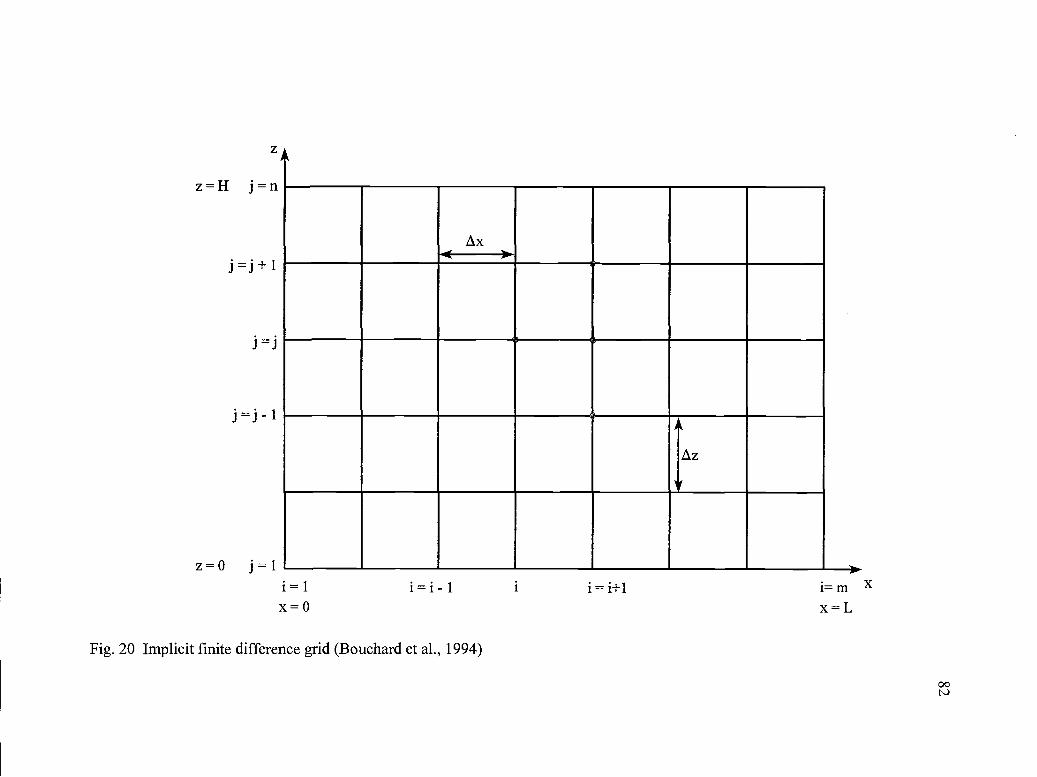
z
z=H j=n
j=j+1
j =j
jj...1
z=O j1i=l i=i-1 1 i=i+1 i=m X
x=O x=L
Fig. 20 Implicit finite difference grid (Bouchard et al., 1994)
LX
jAz

83
Pepper, 1991). The finite element method is very useful in handling problems with
Dirichiet, Neumann, and Robin boundary conditions.
The key step in the finite element analysis is to employ a Galerkin weak statement.
For an x-z 2-dimensional problem, a finite number Taylor (or power) series of known trial
function of x and z can be used to approximate the variables:
n
C(x,z) = Ea41(x,z) (51)j=1
To derive a Galerkin weak statement for the mass transfer equation governing the
membrane filtration process, Eq. 47 can be rewritten as:
L(C)=u- VaC Da2cox HOX H2OX
To achieve a minimized approximation error, the weighted residual must vanish,
that is:
f 4(x,z) L(C)dt=
f 4(x,z) L(C11)dxdz 0 for 1 (53)
The Galerkin weak statement for Eq. 47 becomes:
(52)
The finite element analysis uses a non-overlapping sum of finite element basis

84
2Ae(X3Z1 XiZ3)e + (Z3 -Z1)X + (X1 -X3)y
2Ae(X1Z2 -X2Z1)8 + (Z1 Z2)eX + (X2 -X1)y
(32Ae
(57)
WS= 4lu - Idr10 H3 H2a2)f 4(x,z) L(C)d
(aCl1 vaC" Da2CII
(54)
= f V4 L(C)d - laoL(C)nds
{Nk()} to replace 41(x, z) in the discretized elements in the domain Q and its
boundary Q (Eq. 55).
h(x,z) = C'(x,z) Ue C(x,z)Ce(XZ) {Nk (()}T {c} (55)
Then the finite element discrete approximation to the Galerkin weak statement
becomes:
WSh = Ee l V{Nk} v{Nk}Tdt {C}e(56)
lao {Nk} L(C)nds
In a triangular finite element shown in Fig. 21, defining the local natural
coordinate system spanninge
as (Baker and Pepper, 1991):
(X2Z3 X3Z2)e + (Z2 -Z3)x + (X3 -X2)Y
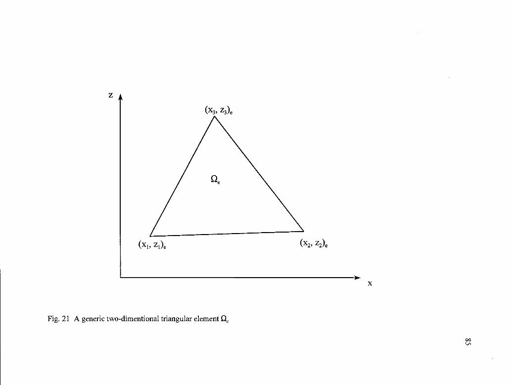
Fig. 21 A generic two-dimentional triangular element e
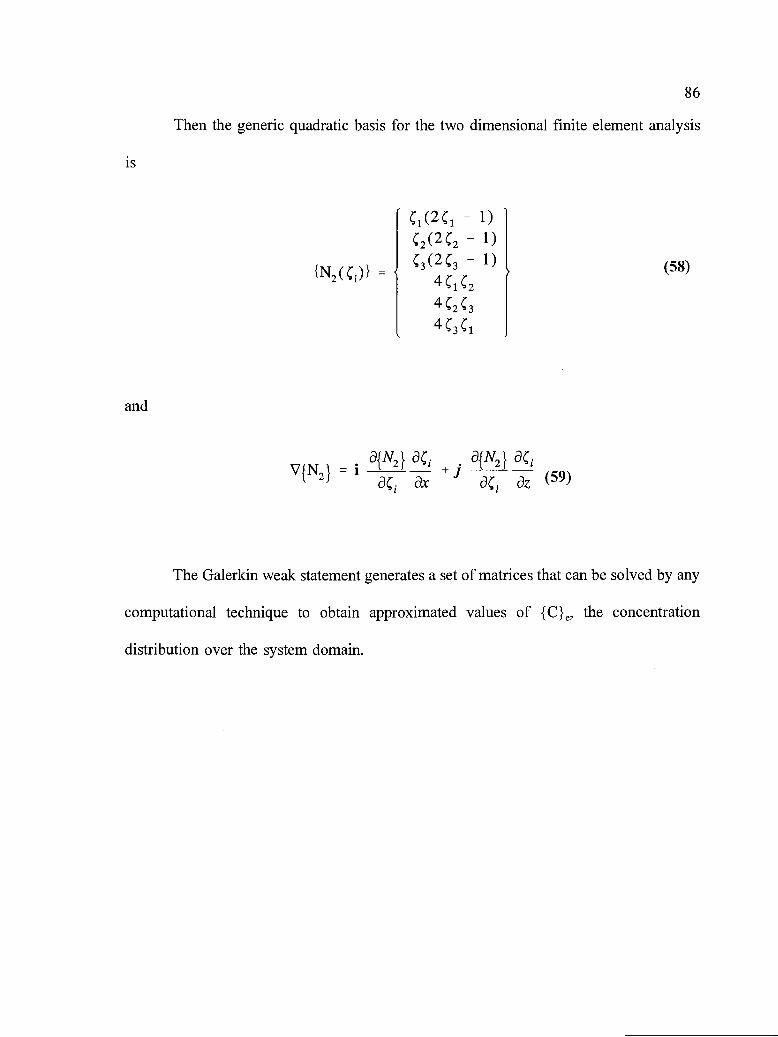
86
Then the generic quadratic basis for the two dimensional finite element analysis
- 1)(2(2(2 - 1)
{N2(()} =(3(2(3 - 1) (58)
4(3
V{N2} =a{N2}a(1
a( 8x 3z (59)
The Galerkin weak statement generates a set of matrices that can be solved by any
computational technique to obtain approximated values of {C}e, the concentration
distribution over the system domain.
is
and

4. MATERIALS AND METHODS
4.1 Characterization of waste water generation in the surimi industry
One plant was selected for this study in the summer of 1994, which was a peak
season for Pacific whiting (Merluccius productus) surimi manufacturing. The plant was
located in a coastal city of Oregon, on the Columbia River. It directly discharged the
waste water into the river without any pretreatment.
To completely understand the waste water generated by this plant, three steps were
taken. The first step was to understand and identify all the unit operations in the surimi
processing line, and to develop a process flow diagram. The second step was to conduct
a water and waste water audit, and to collect waste water samples at selected sampling
points. The third step was to analyze and characterize the waste water generated in the
processing plant.
4.1.1 Process flow diagram development
The surimi processing line was examined to understand the functions of each unit
operation and the relationship between different unit operations. Water supply lines and
locations of waste water generation were identified. A flow diagram of surimi processing
was then developed.
A system approach was adopted. Based on the preliminary observation, it was
found that the whole processing line was treated as a major system with two subsystems
(Fig. 22 and Fig. 23). The first subsystem processed raw fish into minced fish, which
87
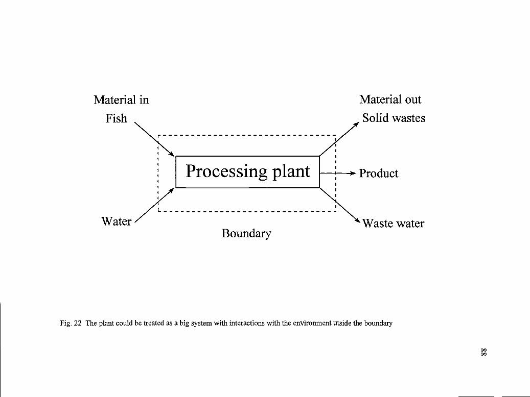
Material in
Fish
Water
Processing plant
Boundary
Fig. 22 The plant could be treated as a big system with interactions with the environment utside the boundary
Material out
Solid wastes
Product
Waste water

Fish
Water
Subsystem ' Mince ) Subsystem 2 Frozen surimi
Solid waste
Waste water
Fig. 23 The big system may be divided into two subsystems that interact with each other through an intermediateproduct, fish mince

90
was then a raw material for the second subsystem. Two subsystems interacted with each
other through the intermediate product, fish mince. Each subsystem was composed of
different unit operations (Fig. 24).
4.1.2 Audit of water consumption and waste water generation
After the flow diagram was developed and sources of waste water were identified,
a 3-day water and waste water audit was conducted using the methods modified from
Mate (1992) and Mannapperuma et al. (1993). Daily measurements of water and waste
water flow rates from each unit operation were conducted, and a 3-day average was used
to represent the water and waste water flow rates.
1. Water audit
Water consumption in the processing lines was determined by measuring the water
flow rate in the pipes using a microprocessor-based ultrasonic water flow rate meter (Fig.
25) manufactured by Polysonics Co. (TYME-FLYTE portable ultrasonic flowmeter,
Model TF-P, Polysonics, Washington, D.C.). This device consisted of two ultrasonic
signal transducers that were mounted on the external wall of the pipes at a distance
determined by the pipe size. The time required for an ultrasonic signal to travel between
the two transducers was measured electronically. The difference in time between signals
traveling upstream and downstream is proportional to the liquid flow velocity. With a
known internal diameter of the pipe, the flow rate could be calculated. This device was
a non-invasive water flow rate meter and could be used to measure the water flow rate

Fig. 24 Each subsystem can contain different numbers of units operations
Main system
Unit 1
Unit2 Subsystem 2
Unit 3

Water flow direction
Upstream signaltransducer
Fig. 25 Schematic diagram of a ultrasonic flow meter
Water pipe
Microprocessor-based ultrasonic flow meter
Downstream signaltransducer

93
in the existing processing lines without interrupting normal operations. When measuring
water flow rate, three determinations were taken at each sampling point.
Some unit operations in surimi processing require a continuous supply of water to
ensure a smooth operation. These operations were almost all located in the raw material
treatment stages (Subsystem 1). Fresh water was supplied to prevent fish body fluids and
fish muscles from sticking to the machines. In washing of fish mince, sequential batch
operation was used. As a characteristic of batch-type operation, water was not
continuously supplied to the washing tanks, but was automatically fed to the tanks
according to the operation sequence determined by the process logic controller (PLC).
In Subsystem 2, batch operations (such as surimi washing) were repeated
periodically. If the time needed to complete a washing cycle was t, and during which
period only a fraction of the time, ta, was used to pump fresh water into a washing tanks,
as graphically shown in Fig. 26 the total amount of fresh water pumped to the washing
tank can be calculated with Eq. 60.
''H2O = X ta(60)
where V1120 = total volume of water used in a washing cycle, L;
QH20, a = flow rate of water when being pumped to the washing tank, L/min.
If water is continuously supplied to a machine (rinsing), Eq. 60 can also be used,
in which ta is equal to t. To analyze the water consumption in a washing batch, it is more
desirable to use an averaged water flow rate to express an overall water flow rate over the

Washing
Dewatering
tIdling Dewatering
ta
Fig. 26 Time distribution in on-off control of batch operation in Subsystem 2
t
Water in Fish mince in Stirring/washing Discharging
ta

95
time period of t. So the averaged water flow rate in a batch, QH2o is expressed as (Eq.
61):
V (61)H20, AVG
The total water consumption in a subsystem is the sum of each individual
operation (component), as expressed in Eq. 62.
Subsystem, i AVG, j(62)
where subscript i represents a subsystem, and j represents a component in that
subsystem containing a total number of n components.
2. Waste water audit
Waste water flow rates were calculated from the volume of the waste water
collected in plastic buckets, divided by the time measured by a stopwatch. For some
operations, such as the heading operation where waste water was scattered all around the
heading machine, more than one bucket was used to collect the waste water within a
specified time period. At each sampling point, measurements were replicated for three
times. The volume of waste water was measured, and the flow rate could be calculated
by Eq. 63:

WH2O, AVG
VWH2O (63)tm
96
where V20 was the volume of waste water collected, and tm is the time needed to collect
the waste water.
In batch-type operations such as the dewatering process where waste water was
intermittently released, equations similar to Eq. 60, Eq. 61, and Eq. 62 were used to
calculate average flow rates of waste water from a unit operation (Eqs. 64 and 65).
QWH2O,AVG - t
X t (64)
Qwio, Subsystem, i Qwio, AvG,(65)
where subscript WH2O represents waste water. In a continuous operation ta was
equal to t.
4.1.3 Chemical analysis
Approximately 1 L of waste water samples was collected at each sampling point.
Samples were kept in a refrigerated container and immediately transferred to a deep
freezer (-40 °C) (Fresenius et al., 1989). Prior to conducting chemical analyses, samples
were thawed overnight in a refrigerator (3-5 °C).
Chemical analyses were conducted to determine total solids (TS), chemical oxygen

97
demand (COD), protein, and 5-day biological oxygen demand (BOD5). TS and BOD5
were measured using the Standard Methods (Greenberg et al., 1980). COD was measured
using the method developed by Hach Chemical Co. (Gibbs, 1979).
4.2 Treatment of surimi wash water by ohmic heating
4.2.1 Ohmic heating device
A batch-type ohmic heating device (Fig. 27) developed by Huang et al. (1996) was
used in this study. A 500 mL beaker containing a 250 g sample was enclosed in a
styrofoam box, and placed on top a magnetic stirrer (Model SP18425,
BarnsteadlThermolyne, Dubuque, IA). The sample was gently stirred with the magnetic
stirring bar to ensure uniform heating. The electric voltage was set at 90 V throughout the
test. Heating temperatures were controlled by a temperature controller (Type E5CS-
R1KJX-520, Omron Manufacturing, the Netherlands B.V.). The sample temperature was
measured with a Type C thermocouple every 5 s and recorded in a datalogger (Model
CR10, Campbell Scientific, Inc., Logon, UT). To measure the current passing through the
samples, an AC current transducer (Model 0M8-2182AFA0, OMEGA Engineering,
Stamford, CT) was used to linearly convert the AC current signals into DC voltages
measurable by the datalogger.

Temperature controller
Type C thermocoupleType J thermocoupleTransformer
SS electrodeStyrofoam box500 mL beaker
Fig. 27 Ohmic heating device for treatment of surimi waste water

U
Le
A
(66)
(67)
99
4.2.2. Calibration of the device and determination of electrical conductivity
To measure the electrical conductivity of surimi wash water, the device was
calibrated with a standard solution with a known electrical conductivity (Palaniappan and
Sastry, 1991 a; 1991 b). Solutions (250 g) of 0.17 M sodium chloride (NaC1) were quickly
heated to 25 °C in the ohmic heating device at 90 Vac, and kept constant at this
temperature. The electrical voltage was quickly reduced to 5 Vac after the temperature
reached 25 °C. The current passing through the solution at 25 °C was measured and
recorded. The effective device coefficient, which is determined by the geometry of the
ohmic heating device, can be calculated from Eq. 66 (Palaniappan and Sastry, 1991 a;
1991b):
K-C
I
where K is the effective device coefficient, defined as:

100
4.2.3 Sample preparation
Pacific whiting fish (500-600g) less than 24 hr postharvest were obtained from a
local surimi processing company. Fish were headed, gutted, filleted, and comminuted into
fish mince Fish mince was mixed with chilled distilled water (fishlwater = 1:3) and
washed for 3 mm under a gentle mixing condition. After washing, the mixture was
filtered consecutively through two stainless steel strainers (hole diameters 2 mm and 1
mm, respectively) to remove fish mince. The wash water was stored in a cold room (5
°C) and subjected to ohmic heating the same day.
4.2.4 Coagulation offish proteins by ohmic heating
Wash water samples (250 g) were heated to 30, 40, 50, 60, 70, and 80°C,
respectively, using the method described by Huang et al. (1996). After heating, samples
were quickly cooled to below 5°C in an ice bath to retard the enzymatic degradation.
Samples were centrifuged at 1700 x g for 10 mi Supernatants were collected for
chemical analyses. All tests were run in triplicate.
4.2.5 Chemical analysis
Total solids (TS), total suspended solids (TSS), protein concentration, and
chemical oxygen demand (COD) were analyzed. TS and TSS were measured using
Standard methods (Greenberg at al., 1980). After the samples were solubilized in 5%
sodium dodecylsulfate (SDS) solution (Lin et al., 1995), protein content was determined
by the method of Lowry et al. (1951) with bovine serum albumin (BSA) as the standard.

101
COD was assayed using the method developed by Hach Chemical Co. (Gibbs, 1979).
Sodium dodecylsulfate polyacrylamide gel electrophoresis (SDS-PAGE) was employed
using the method modified from Laemmli (1970) to evaluate the effect of heating on
protein coagulation. Samples (100 jig) were mixed with a treatment buffer containing 1-
ME at 1:1 (v/v) and loaded to the gel. SDS-PAGE was conducted at room temperature
using 20 mA current overnight. The gel was stained with 0.125% Coomassie brilliant
blue R-250 and then destained.
4.2.6 Enzyme assay
Protease activity was assayed using the method described in An et al. (1 994b)
using casein as substrate. Wash water samples (200 tL) with and without ohmic heating
were mixed with 500 g of casein and 1000 jtL of Mcllvaine's buffer (pH 5.5) containing
1 mM J3-mercaptoethanol (13-ME), and incubated at 55°C for 1 hr. The reaction was
terminated by adding 500 pL ice-cold 50% (w/v) trichloride acid (TCA) solution. Blanks
were prepared by adding TCA solutions to the samples prior to incubation. TCA-
coagulated proteins (unhydrolyzed) were allowed to precipitate for 15 mm at 4 °C, and
centrifuged at 5000 x g for 10 mm. Supernatants (800 L) mixed with 200 tL 5 N
NAOH solution were assayed for tyrosine(Tyr) concentration using the Lowry's method
(Lowry et al., 1951). Specific activities of proteases were expressed as nmol Tyr/min per
mg of protein.

4.3. Microfiltration of surimi wash water
4.3.1 Membrane filtration unit
A stainless steel plate-and-frame crossflow membrane filtration unit was fabricated
and installed (Fig. 28). The unit had a channel height of 7.934 x iO m (5/16 inches) and
a filtration area of 0.03 m2 (6 x 8 inches). An air-driven double diaphragm pump (Model
BK-5, All-Flo Pump Co., Mentor, OH) was used to pump the feed into the filtration unit.
To achieve a pulseless flow during filtration, a flow stabilizer (Model Sentry II, Blacoh
Fluid Controls, Moreno Valley, CA) was mounted at the exit of the diaphragm pump.
A rotameter (Model FL7304, OMEGA Engineering, Inc., Stamford, CT) was installed to
measure the flow rate of the feed. Two pressure sensors (Model PX236-100G V,
OMEGA Engineering, Inc., Stamford, CT) were installed in the inlet and outlet of the
filter to measure and monitor the applied pressures. The permeate was collected in a pre-
weighed plastic bucket and the weight was continuously measured by a loadcell (Model
LCL-010, OMEGA Engineering, Inc., Stamford, CT). The sample and ambient
temperatures were measured by Type T thermocouples. A datalogger (Model CR1OX,
Campbell Scientific, Inc., Logan, UT) was used to collect the real time data of pressures,
permeate weight, and temperatures. The datalogger was programmed to collect the data
at variable sampling rates (every 5 s for the first 30 mm, every 1 mm for the next 1 h,
and every 5 mm for the rest of filtration process). The filtration data were transmitted to
a notebook computer through the I/O port of the datalogger, and the process was
monitored by the PC.
102

r
CR-10X
Datalogger
2N
Sc
-II
Permeate tank
Rotameter
Flow stabilizer
V
Air-drivendiaphragmpump
Pressure sensorTop plateSpacer and gasketsMembraneSupport plateBottom plate
Fig. 28 A plate-and-frame crossflow membrane filtration unit with a data acquisition system.
Feed tank

104
4.3.2 Preparation of samples
Fresh Pacific whiting (< 24 h post harvest) were obtained from a local surimi
processing plant in Warrenton, Oregon. Fish were manually headed, gutted, and
comminuted into fish mince in a Hobart meat grinder (Model K5SS, Hobart Co., Troy,
OH). Fish mince was mixed with chilled ( 3°C) distilled water (w/v 1/3) and washed
for 3 mm under a gentle mixing condition at ambient temperature. Wash water was
strained through 2 stainless steel strainers (hole diameters 2 mm and 1 mm, respectively).
Approximately 12 L of wash water was obtained and used in each test. Wash water was
mixed with 20 ppm silicone antifoam (Antifoam 1510-US, Dow Corning, Midland, MI)
to prevent foam formation during pumping. To evaluate the effect of solid concentration
on pore blocking and cake formation, solutions with different concentration were
prepared.
4.3.3 Membranes
Polysulfone (Supor 20 and Supor 45, with pore sizes 0.2 and 0.45 j.tm,
respectively) and polyethersulfone (HT 20 and HT 45, with pore sizes 0.2 and 0.45 jtm,
respectively) membranes were purchased from Gelman Sciences Inc. (Ann Arbor, MI).
4.3.4 Characterization of membranes
Two parameters, specific flux and membrane resistance, were used to
macroscopically characterize the membranes. To characterize membranes, deionized water
(>16 M) was pumped into the membrane unit. Volumes of the permeate through the

105
membrane were measured for calculation of the flux (L/m2s). Specific flux J (L/m2s Pa)
was defined as the pure water flux through the membrane per unit area (m2) per unit
pressure (Pa). Membrane resistance Rm can be calculated from Eq. 12 when pure water
was used in filtration. The viscosity of water was chosen as 0.00 1 PaSs.
4.3.5 Filtration process
Surimi wash water was pumped from the feed tank to the filtration unit at 19
L/min (5 GPM) under an average transmembrane pressure of 34.5 KPa (5 psi). The
retentate was recycled back to the feed tank. To simulate a continuous filtration process
(constant feed concentration), the total permeate weight was controlled at less than 5%
of the total feed weight so that the increase in the feed concentration could be neglected
(Redkar and Davis, 1993). The filtration temperature was controlled at 12 - 15°C
throughout the tests. Samples of feed, permeate, and concentrate were collected for
chemical analyses.
4.3.6 Chemical analysis
Samples of feed, permeate, and concentrate were collected for chemical analyses
of TS, TSS, protein, and total ash. TS, TSS, and ash were measured according to the
Standard Methods (Greenberg et al., 1980). Total organic solids (TOS) was calculated
from the difference between TS and ash. Biuret method was used to detect protein
concentrations in the samples with solubilized caseinate as the standard. The protein
content of caseinate was calibrated using the Kjedahl method (AOAC 1995) using a
106
conversion factor of 6.38.
To understand the components in the wash water samples that passed through the
membrane pore, sodium dodecylsulfate polyacrylamide gel electrophoresis (SDS-PAGE)
was performed using the method modified from Laemmli (1970). A Bio-Rad vertical
electrophoresis unit (20 x 20 x 0.08 cm) was used. Samples of 100 pg were loaded to
10% polyacrylamide gels. From the band patterns of the gels, it was possible to
understand the molecular weight ranges of protein components in the wash water samples
passing through the membrane pores.
4.4. Finite element analysis of concentration polarization during ultrafiltration of
bovine serum albumin
4.4.1 Membrane filtration unit
A small scale stainless steel (SS 304) radial crossflow plate-and-frame membrane
filtration unit was designed and fabricated. It was composed of two separate parts, a top
section (Fig. 29) and a bottom section (Fig. 30). A stainless steel screen (200 mesh) disk
was placed in the bottom section to provide a mechanical support to the membrane.
Polysulfone ultrafiltration membrane disks (MWCO=30,000 Dalton), obtained from
Millipore Corp. (Biomax-30, lot No. P5HM0882) was positioned on top of the stainless
steel screen. The membrane was 47 mm in diameter with an effective filtration area of
11.4 cm2 after installation in the filter housing. A new membrane was used for each test.

Fig. 29 Top section of a radial crossflow filter
11/16"
01-17/20"

3/4"
Fig. 30 Bottom section of a radial crossflow filter

109
A gear pump was used to pump and pressurize the feed solution into the filter unit. The
feed was pumped into the center port of the top section and flowed radially across the
filter, and exited the filter in the exit port shown in Fig. 31. The inlet and outlet
pressures were measured by two pressure sensors (Model PX236-100G V, OMEGA
Engineering, mc, Stamford, CT). The transmembrane pressures were adjusted by a valve
installed in the outlet of the membrane filter. The permeate was collected in a small
plastic bottle, and weighed by a loadcell (Model CLC-454G, OMEGA Engineering, mc,
Stamford, CT). A datalogger (Model CR1 OX, Campbell Scientific, Inc., Logan, UT) was
used to collect the real time data of pressures, permeate weight, and temperatures. The
datalogger was programmed to collect the data at every 5 s throughout the filtration
process. The filtration data were transmitted to a notebook computer through the I/O port
of the datalogger, and the process was monitored by the PC.
BSA (68,000 Dalton, Sigma A7906, Fraction V Powder) solutions were prepared
by dissolving 0.25 g dry powder in 1 L of pH 6.0 0.05M Mcllvaine's buffer and O.l5M
sodium chloride solution. Freshly prepared BSA solution was used in the tests.
4.4.2 Finite element analysis of concentration polarization during ultrafiltration
Since BSA molecules are larger than the MWCO membrane, complete rejection
was observed and experimentally verified. If the BSA molecules are regarded as rigid
spheres, the mass transfer is governed by Eq. 47. With known boundary conditions and
diffusion coefficient, the convection-diffusion mass transfer equation can be solved
numerically.

/\Feed tank
Membrane
Pump
Gasket
CR10Datalogger
Laptop computer
Feed
Loadcell
Fig. 31 A radial crossflow ultrafiltration unit with a computer-assited data collection system
VA Retentate
Permeate collector
Porous supportPermeate

111
Since the filtration unit is a radial crossflow device, the x coordinate in Eqs. 25-27
must be replaced by the radius r (Ganguly and Bhattacharya, 1994). Eq. 47 becomes
aC vC DäCU + - = -ar HaA HaA2
The boundary conditions for Eq. 68 are:
at r = 0, C = C0
at A 0, = 0
acat A = 1, =_! C.A D
In the radial crossflow membrane, the fluid flow velocity changes as a function
of radius, i.e.,
Qo (70)2 c rH
as:
In a discretized domain, the velocity profiles of Eqs. 45 and 46 can be rewritten

Re
70
v(r,) = J(r1) ( 3X2 - + ( -4A7 + 14A6 - 21 + 27 - 162)70
4.4.3 Finite element analysis
A Windows 95 based finite element analysis package called Pdease2DTM
developed by Macsyma, Inc. (Arlington, MA) was chosen for simulation of concentration
polarization during ultrafiltration. Pdease2D is a general purpose two dimensional finite
element analysis program for obtaining numerical solutions to steady or non steady state
boundary value, time-dependent boundary value, initial value, and eigenvalue problems.
It uses the Galerkin statement with quadratic basis to convert continuous partial
differential equation into discrete nodal equations. It features automatic mesh generation
and adaptive grid refinement, and can handle linear and nonlinear problems. It can
generate a series of output graphics after numerical computation.
In finite element analysis, normalized coordinates were used to transform the
membrane flow channel into a dimensionless square region with each side having a length
of one. In the region near the membrane surface, more meshes were placed using a
112

113
command called "feature" in Pdease2DTM. The average effective diffusion coefficient D
of BSA molecule was assumed constant, and was chosen as 3.5 x 10b0 rn/s (Kleinstreuer
and Paller, 1983). The osmotic pressure as a function of BSA concentration was obtained
from Viker et al. (1981). Simulations were completed in Cyrix P-200 computer within
30 mm.

5. RESULTS AND DISCUSSION
5.1. Characterization of waste water generation in the surimi industry
5.1.1 Process flow diagram
The audit of water and waste water was conducted in a shore-based surimi
processing plant. Therefore, the results of this study are pertinent to the shore-based
surimi operations only. Fig. 32 is a detailed flow diagram of the surimi processing line.
The surimi processing line was treated as a system with two interacting subsystems Fig.
33 and Fig. 34. Each subsystem was composed of unit operations that were closely related
to each other.
5.1.1.1 Subsystem 1 - raw material treatment
Raw fish were caught off the coast of Oregon and transported to the plant for
processing. Fish were conveyed from the fishing boat in the receiving dock through a
pipe via sea water and stored in four 50,000-pound storage tanks. Most of the sea water
was returned to the sea. Fish in the storage tanks were immersed in the sea water that
provided lubrication and was a conveying agent when fish were released to the feeding
tank located in the bottom of the storage tanks.
A conveyor belt was used to transport the fish from the feeding tank to the
heading machine Each fish was properly aligned on the conveyor belt by the operators
for the heading operation. In the heading machine, fish heads were separated from the
114

Refiner
Packaging
+Freezing
>1
> Surimi
Fig. 32 Flow of materials and sources of waste water.
T A Waste mince
Waste water
ti Waste water
Rotary screen dehydrator I
Waste water
Rotary screen dehydrator 2
L_:i:... Waste water
Ca)
a)C0.0Ca)
0)U)-DCSa)I
47
Seawater
-
Cs
0)C
a)a)LL
Fresh water
seawater
I-0 LCs CS C) L.
>
I stwashingf___J Mincing <J
Gutting
V Waste water, guts
Waste water, bones

Water Fish
c1V
Holdingtank
Feedingtank
1
Headingmachine
Guttingmachine
Mincingmachine
Fig. 33 Unit operations in Subsystem 1
Guts Grinder
Solid waste Waste(byproduct) water
116
IFish mince

First washing
4'
4;.
1stWDC
First dewatering
Second washing
Second dewatering
4
*
First rinsing/rotary screen
Third washing41
Third dewatering
Second rinsing/rotary screen
Refining
Screw press
4'
Mixing, packaging, & freezing
11
Frozen surimiFig. 34 Unit operations in the 2nd subsystem
3rdWDC
*Washing..dewatering cycle
Solidwaste
Waste water
Water rFish mince
117
4' 2nd WDC

118
fish bodies. The gutting machine removed the fish guts. The mincing machine removed
skins and bones while mincing took place.
In the heading, gutting, and mincing operations, water was supplied to the
machines to perform two functions. Water streams were injected to the cutting blades to
clean the blades and to provide lubrication for smooth operations. Running water was
used to flush the separated fish body parts (heads, guts, and skins) out of the machines.
Estimated fish mince production rate was 29.1 kg/mm, which was about 32% of the total
fish fed into the production line. This value was very close to the published values
(Babbitt et al., 1985; Lee, 1986).
5.1.1.2 Subsystem 2 - surimi processing
This subsystem contained three washing, three dewatering, two rinsing, one
refining, one screw pressing, and one final product preparing (including mixing,
packaging, and freezing) operations (Fig. 34). Fish mince received from Subsystem 1 went
through three washing-dewatering cycles (WDC) in the plant, and was finally processed
into frozen surimi. A more detailed explanation of each unit operation functions can be
found in Lee (1985), Regier et at. (1985), Swafford et al. (1985), and Toyoda et al.
(1992). In refining and screw pressing operations, the solid waste was pumped to the
grinder in Subsystem 1.
Sequential batch operations were used in Subsystem 2. Surimi processing started
with a batch of fish mince received from Subsystem 1, and continued sequentially in the
processing line. Each unit operation was operated in an "on-off' manner controlled by

119
the process logic controller. When fish mince was pumped to the machines, an operation
(such as washing and dewatering) was accomplished ("on" mode), and after that machines
remained inactive ("off' mode) until the next batch of fish mince entered the machines.
A continuous operation in Subsystem 2 was achieved with many sequential batch
operations working at the same time (Fig. 2).
5.1.2 Water and waste water audit
5.1.2.1 Subsystem 1
Table 10 lists flow rates and characteristics of the waste water in the subsystem.
The flow rates of solid wastes (COD, BOD5, and TS) are listed in Table 11. These two
tables show that gutting and mincing operations generated most of the waste water in
Subsystem 1. The gutting operation contributed to the majority (>65%) of solid wastes.
Although the flow rate of the waste water discharged in transferring the fish guts was not
the highest due to high concentration of solids in the waste water, the flow rates of solid
wastes (COD, BOD5, and TS) were the highest among all the waste water sources in
Subsystem 1. This is reasonable since the body fluid from the broken internal organs
contained soluble materials that could be easily dissolved in the water. COD/BOD5 of the
waste water was approximately 2. In the mincing operation, part of the injected fresh
water became wash water in the first washing tank. Only transferring water was
discharged from the mincing operation. Since all fresh water entering this subsystem
became waste water, the flow rate of fresh water was equal to that of waste water (192.3

Table 10 Flow rates and characteristics of waste water generated in Subsystem 11
Unit operations Flow rate (L/min) COD (gIL) BOD5 (gIL) TS (gIL)
Subtotal Waste water flow rate = 192.3 ± 20.2 (Llmin)Assuming that the operations were not interrupted.
2 valueStandard deviation
" Water injected to the cutting bladesWater used to transfer heads, guts, and skins out of the machines
Heading CB4 14.92 ± 1.3 6.54 ± 0.07 4.43 ± 0.07 3.97 ± 0.19
T5 8.94 ± 0.96 6.47 ± 0.31 2.75 ± 0.18 3.78 ± 0.07
Gutting CB 58.7 ± 12.4 5.42 ± 0.16 2.11 ± 0.33 3.81 ± 0.15
T 30.4 ± 5.9 36.57 ± 1.93 18.89 ± 0.44 23.92 ± 0.30
Mincing T 79.4 ± 14.7 6.54 ± 0.58 3.54 ± 0.45 5.30 ± 0.22

Table 11 Averaged solid waste flow in the waste water generated in Subsystem 1
Unit operations COD (kg/mm) BOD5 (kg/mm) TS (kg/mm)
Heading CB 0.097 ± 0.009 0.066 ± 0.006 0.059 ± 0.006
T 0.058 ± 0.007 0.025 ± 0.003 0.034 ± 0.004
Gutting CB 0.3 18 ± 0.068 0.124 ± 0.033 0.223 ± 0.048
T 1.112±0.224 0.574±0.112 0.727±0.141
Mincing T 0.519 ± 0.107 0.281 ± 0.063 0.421 ± 0.080
Subtotal 2.10 ± 0.25 1.07 ± 0.13 1.46 ± 0.16

122
± 20.2 L/min) High variations in the waste water flow rates could be explained by the
variations in feeding machine operators.
The feeding rate of raw fish to the heading machines was measured as 91.9 ± 18.0
kg/mm. Approximately 2 kg of waste water was generated for every kg of raw fish
processed in the heading, gutting, and mincing stage. For every kg of raw fish processed,
the estimated amount of COD, BOD5, and TS generated would be 0.023 ± 0.005, 0.0 12
± 0.003, and 0.016 ± 0.004 kg/kg fish, respectively. Amount of water used for
transferring solid wastes (heads, guts, skins, and bones) increased significantly as the
operation proceeded (Table 11). Among the three operations, the smallest amount of
fresh water ( 15 L/min) was used to flush fish heads (the largest in physical size) out of
the heading machine, while the mincing operation consumed the largest amount of water
( 90 L/min) Considerable amount of water could be saved if the water used for
transferring solid wastes is reduced in gutting and mincing operations.
5.1.2.2 Subsystem 2
Minced fish was sequentially transferred through several stages of washing and
dewatering before feeding to the screw press. The first washing operation was a
continuous process, and all the other unit operations were sequentially operated in batch
style. To maintain a continuous operation in the production line, different numbers of
washing tanks were involved in the second and third washing processes (Table 12). The
washing time increased as washing cycles progressed (Table 13). Dehydration
(dewatering) times were relatively consistent in the second and third dewatering operations
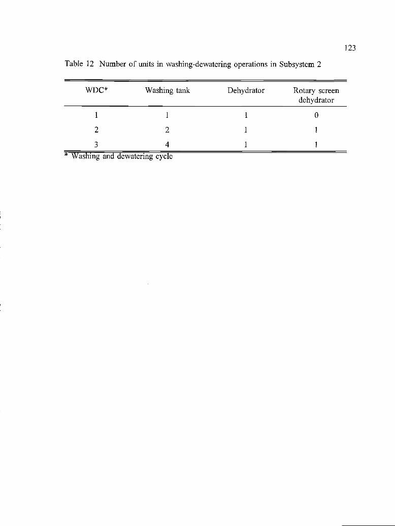
Table 12 Number of units in washing-dewatering operations in Subsystem 2
* Washing and dewatering cycle
123
1 1 1 0
2 2 1 1
3 4 1 1
WDC* Washing tank Dehydrator Rotary screendehydrator

Table 13. Time distribution in washing-dewatering operations in Subsystem 2
ta* t**(min) (mm) tta (mm) t
ta represents the raction o time in a cycle o a batch neede. to comp ete a unction suc as washing, dehydrating, orinsing..
* * t represents the time needed to complete a cycle in a batch operation.
(mm) ta (mm)
1 2.29±0.16 2.29 ± 0.16 0.88 ± 0.03 2.30 ± 0.06 0 0
2 3.43 ± 0.09 8.41 ± 0.46 2.26 ± 0.10 6.61 ± 0.88 2.50 ± 0.28 6.61 ± 0.88
3 8.44±0.13 13 .33±0.3 5 2.14 ± 0.30 5.13 ± 0.95 2.30 ± 0.01 5.13 ± 0.95
WDC Washing tank Dehydrator Rotary screen dehydrator
125
(both in high speed dehydrators and rotary screen dehydrators). In each washing
operation, water to fish mince ratio was approximately 3 to 1. Averaged water
consumption was the highest in the first washing operation, followed by the second and
third washing. Water streams were continuously injected to the rotary screen dehydrators,
even when these units were in the "off' mode, leading to increased water consumption.
If water streams were injected to the rotary screen dehydrators only when fish mince was
pumped, a considerable amount of water (about 90 L/min) could be saved. Since two
rotary screen dehydrators were used in the third WDC, more water was used to rinse the
fish mince (Table 14).
The high speed dehydrator in the second WDC generated the highest flow of waste
water, followed by those in the first and third WDCs (Table 15). Due to continuous
water streams injected to the rotary screen dehydrators, averaged waste water flow rates
were higher than those generated in the high speed dehydrators. The levels and amount
of COD, BOD5, and TS were the highest with the waste water generated from the first
high speed dehydrator (Tables 16 and 17). Among three WDCs, more than 50% of the
solid wastes (COD, BOD5, and TS, kg/mm) were generated in the first high speed
dehydrator. Although relatively high in the concentrations of COD, BOD5, and TS
generated in the final screw press (Table 18), averaged flow rates of waste water and solid
waste (kg/mm) were not very high when compared with waste waters generated in the
three preceding WDCs.
The total waste water generated from Subsystem 2 was 328.8 ± 21.9 L/min. If
50% of fish mince was processed into frozen surimi (9.7 kg/mm), then about 34 L of

Table 14 Water consumption in a single washing and rinsing operation
WDC
* Averaged water flow rate based on one washing tank.
Washing Rotary screen dehydrator
QH20,a (L/min) QH2O, avg (L/min) Q112o,a (L/min) QH2O, avg (Llmin)
1 89.1 ± 5.5 89.1±5.5 0 0
2 447.1 ± 2.3 68.0 ± 37* 34.7 ± 4.7 34.7 ± 4.7
3 447.1 ± 10.6 23.1 ± 0.8* 58.9 ± 5.6 58.9 ± 5.6
Subtotal 3 17.5± 9.8 93.6 ±7.3
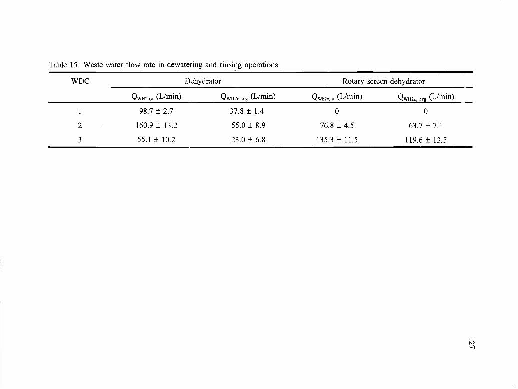
Table 15 Waste water flow rate in dewatering and rinsing operations
WDC Dehydrator Rotary screen dehydrator
QwH2o,a (L/min) Qwi12o,avg (L/min) Qwh20, a (L/min) QwH20, avg (L/min)
1 98.7 ± 2.7 37.8 ± 1.4 0 0
2 160.9 ± 13.2 55.0 ± 8.9 76.8 ± 4.5 63.7 ± 7.1
3 55.1 ± 10.2 23.0 ± 6.8 135.3 ± 11.5 119.6 ± 13.5
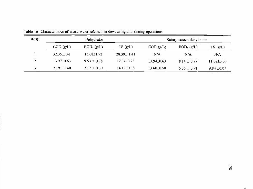
Table 16 Characteristics of waste water released in dewatering and rinsing operations
WDC Dehydrator Rotary screen dehydrator
COD (gIL) BUD5 (gIL) TS (gIL) COD (gIL) BOD5 (gIL) TS (gIL)
1 32.35±1.41 15.68±1.73 28.39± 1.41 N/A N/A N/A
2 13.97±0.63 9.53 ± 0.78 12.34±0.28 13.94±0.63 8.14 ± 0.77 11.02±0.00
3 21.91±1.40 7.17 ± 0.39 14.17±0.38 13.60±0.58 5.36 ± 0.91 9.84 ±0.07

Table 17 Averaged solid waste generated in dewatering and rinsing operations
WDC Dehydrator Rotary screen dehydrator
COD (kg/mm) BOD5 (kg/mm) TS (kg/mm) COD (kg/mm) BOD5 (kg/mm) TS (kg/mm)
1
2
3
1.39 ± 0.08
0.34 ± 0.06
0.24 ± 0.06
0.67 ± 0.08
0.23 ± 0.04
0.08 ± 0.02
1.22 ± 0.08
0.30 ±0.05
0.15 ± 0.04
N/A
0.16 ± 0.02
0.36 ± 0.07
N/A
0.09 ±0.02
0.14 ± 0.04
N/A
0.13± 0.02
0.26±0.05

130
Table 18 Characteristics of waste water and solid waste flow from final screw press*
* ta 7.8 ± 2.2 (mm), t 10.1 ± 2.2 (mm), QWH2O, a = 38.5 ± 3.1 (L/min),Q120, avg = 29.7 ± 10.9 (L/min)
Name of waste Concentration (gIL) Flow rate (kgIL)
COD 20.50 ± 0.08 0.08 ± 0.02
BOD5 14.53 ± 0.42 0.06 ± 0.01
TS 13.20 ± 0.14 0.05 ± 0.01

131
waste water was generated to make 1 kg of surimi from fish mince. Estimated solid
waste (COD, BOD5, and TS) generated would be 0.27, 0.13, and 0.21 kg/kg of surimi,
respectively. Overall, the BOD5 generated was about 50% of COD. If the processing was
not interrupted, 473 m3 of waste water was generated in Subsystem (Table 19).

Table 19 Summary of waste generation in Subsystem 2
Name of waste Flow rate
Waste water 328.8 ± 21.9 L/min
COD 2.57 ± 0.14 kg/mm
BOD5 1.27 ± 0.10 g/min
TS 2.06 ± 0.12 kg/mm
132

133
5.2 Treatment of surimi wash water by ohmic heating
The relationship between heating time and temperature (Fig. 35) followed a second
order polynomial model, which can be expressed as
T = 11.1 + 0.0499t + 4.639x10⁵ t2, (R2 = 0.995). (73)
This result is in agreement with a similar study in which frozen fish mince wash
water was used as the research subject (Huang et al., 1996). The constant term in Eq. 73
is related to the initial temperature of the samples. This model also suggests a linear
heating rate (dT/dt) during the heating process, which may vary with the feed and applied
voltage.
Electrical conductivity (a) of wash water samples increased linearly with the
heating temperature (Fig. 36). The relationship between electrical conductivity (cT) and
temperature T was best fitted with a linear model (Eq. 74). An increase in is attributed
to reduced electrical resistance at elevated temperatures. The intercept of this equation
represents the electrical conductivity at 0°C, and slope is the rate (d/dt) at which
changes with temperature.
a = 0.353 + 0.0106 T ( R = 0.993 ) (74)
The initial concentrations of solids in wash water samples were 9.341 ± 0.137,
16.72 ± 0.22, 11.449 ± 0.090, and 1.366 ± 0.003 gIL, for protein, COD, TS, and TSS,
respectively. After centrifugation (without heat treatment), these values dropped slightly
to 8.948 ± 0.076, 16.17 ± 0.26, 10.875 ± 0.043, and 0.957 ± 0.079, for protein, COD, TS,
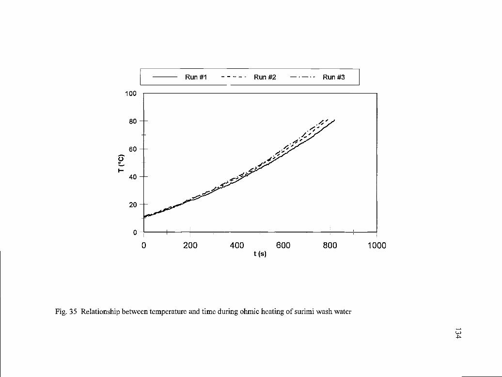
100
Run#1 ----- Run#2 - Run#3
0 200 400 600t (s)
800
Fig. 35 Relationship between temperature and time during ohmic heating of surimi wash water

1.4
>O.8
0.6
- 0.4C.)
Repi Rep2 Rep3
Fig. 36 Electrical conductivity increased linearly with temperature
a = 0.353 + 0.0106 T, R2 = 0.993
10 20 30 40 50 60 70 80 90
T (°C)

136
and TSS, respectively. Heating to 30°C did not cause significant changes in solids
concentration. At higher temperatures, heating caused heat-sensitive proteins to coagulate,
leading to depletion of the solid concentration in the supernatants (Fig. 37). More than
80% TSS was removed at 40°C, indicating that larger particles are more sensitive to heat
treatment and easier to precipitate by heat (Fig. 38). Above 60°C, more than 90% TSS
was removed. Due to the presence of soluble solids such as minerals and other heat stable
substances, reduction in TS was not as significant. Only slightly higher than 70% TS was
removed at temperatures above 60°C while removal of proteins was observed higher than
80%. Reduction in protein concentration may be atttributed to coagulation and enzymatic
degradation by the proteases during heating. The relationship between the residue solid
concentration and heating temperature can be modelled by Eq. 75. Coefficients for each
solid (protein, COD, TS, and TSS, respectively) can be found in Table 20.
C = a1 + a2 T +T
(75)
Effects of ohmic heating on the removal of proteins can be visually observed in
the SDS-PAGE study (Fig. 39). Centrifugation without heat treatment and at low heating
temperatures did not significantly affect the residual composition, since the SDS-PAGE
band patterns are very similar between C and CT. When samples were heated to 50°C,
two bands, one around 43,000 Dalton, and the other one between 20,000 and 30,000
Dalton began to disappear. At 60 °C, bands around 94,000, and in the ranges between
20,000 and 30,000 Dalton disappeared. At higher temperatures (>70°C), heat substantially

20
15J
-C
0(05
0
30 40 50 60T (°C)
Fig. 37 Residual solids concentration decreased with temperature
- Protein COD TS x TSS
70 80

Fig. 38 Percent reduction of solids increased with temperature
-.-- Protein -p-- COD -.-- TS -h-- TSS
10 20 30 40 50 60 70 80T (°C)

Table 20 Coefficients for Eq. 75 for predicting the relationship between residualconcentration and heating temperature
139
Solids a1 a2 a3 R2
Protein -11.0 0.0669 526 0.980
COD -23.2 0.179 1012 0.975
TS -10.83 0.0783 602.0 0.930
TSS -2.56 0.0202 84.8 0.938

Low MW Std
94K
67K
43K
30K
20K
C CT 30 40 50 60 70 80 60' 70' 80'
High MW Std
205 K
116K97K
67K
45 K
29K
Fig.39 SDS-PAGE of ohmically treated surimi wash water samples.. C: Control; CT: Centrifuged; Lanes 30-80 areheating temperatures (sample load = 100 tg); Lanes 60'-80' are the same as Lanes 60-80 with only 60 igsamples loaded.

141
damaged the proteins present in the samples, since only one band (45,000) is visible at
70°C, and essentially no clear protein bands are visible at 80°C. Although no protein
bands are still visible after treatment at temperatures above 70°C, the presence of proteins
was still detected by the Lowry method. A possible explanation to this observation is that
these proteins were small molecules having molecular weights less than 20,000 Dalton.
These results are in direct agreement with the previous research (Huang et al., 1996).
Protease activity (6.169 ± 0.002 nmol/minmg) was found in the control samples.
Since some enzymes may have been removed along with other solids in the samples after
being centrifuged at 1700 x g without heat treatment and after heating to 30°C, a slightly
decreased enzyme activity was observed (Fig. 40). However, at higher temperatures
(>40°C), the enzyme activity began to increase. Between 30 and 60°C, the enzyme
activity increased linearly with the temperature. At 70 and 80°C, low enzyme activity was
observed since heat almost completely destroyed the proteins in the wash water. Enzyme
activity of samples after heating to 60°C was almost 3 times that of the control. This
should be the highest temperature that can be used to preserve the protease activity.
When recovering proteolytic enzymes from the surimi waste water, heat coagulation can
be used to preferentially remove contaminants, while preserving the heat stable proteases.

20
0
Control
aCl) Centrifuged, without heating
I I
10 20 30 40 50 60 70 80
T (°C)
Fig. 40 Specific activity of proteolytic enzymes increased upon heating (<60°C) and decreaseddramatically at T> <60°C.

5.3 Microfiltration of surimi wash water
5.3.1 Effect of membranes on permeate flux and rejection coefficient
Microfiltration membranes may differ in pore sizes, pore size distribution, number
of pores per unit area, and thickness. Macroscopically, the characteristics of membranes
may be determined by filtering pure water through the membranes. Table 21 shows the
characteristics of the membranes. Membranes with 0.45 tm pore size (S45 and H45)
showed a higher specific flux and lower membrane resistance than the membrane with
0.20 tm pore size (S20 and H20). For the 0.45 tm membranes (S45 and H45), very
little difference in J* and Rm was observed. However, pure water flux of S20 membranes
had twice as much specific flux as that of H20 membranes, indicating that S20
membranes are higher in pure water permeability than H20 membranes.
Microfiltration of surimi wash water started with a high initial flux, and then the
permeate fluxes declined rapidly with time, and finally a quasi-steady state filtration was
observed (Fig. 41). The total volume of permeate accumulated rapidly in the first few
minutes of filtration, and increased at a slower rate (Fig. 42). This process is typical for
crossflow membrane filtration. The steady state permeate flux was around 20-22 L/m2hr
for all membranes. Apparently, membranes with larger pore sizes (0.45 tm) had higher
initial fluxes than the ones with smaller pores (0.20 tm), as shown in Fig. 41.
Since TSS was measured by passing the wash water samples through 1.0 jtm glass
fiber filters, while the pore size of membranes chosen in this study were smaller than 1.0
tm, no TSS was detected in the permeates. Except for the ash, concentrations of solids
143

Table 21 Characteristics of microfiltration membranes
S20 = Supor 20, S45 = Supor 45, H20 = HT 20, and H45 = HT 45
144
Membranes' Pore sizeQim)
Specific flux J (L/m2-Pa) Resistance Rm (m2/L)
S20 0.20 4.53 x i0 ± 7.52 x 10⁶ 2.29 x iO ± 3.68 x iO
S45 0.45 7.73 x l0 ± 8.73 x 10⁶ 1.31 x iO ± 1.55 x i05
H20 0.20 2.23 x iO ± 4.60 x 10⁶ 4.60 x io ± 6.26 x iO
H45 0.45 7.86 x iO ± 1.48 x iO 1.29 x io ± 2.10 x i05

0.14
0.12
0.1C')
0.08
Fig. 41 Changes in permeate flux as a function of filtration time for four different types of microfiltration membranes
0 200 400 600
t (s)800 1000

0.6
.1)
E05
0.4
0.3ci)
ci)4-I
E0.1C.)C-)
n
0 500 1000 1500 2000 2500
t (s)
Fig. 42 The accumulated permeate volume increased rapidly at the first few minutes and then increased slowly with time.

147
in the permeates were reduced to different degrees (Table 22). H45 membranes show the
smallest rejection coefficients (Table 23). To evaluate the effect of membrane materials
and pore sizes on the permeate flux and apparent rejection coefficient, statistical analysis
was conducted. The membrane pore sizes and materials had no significant effect (p>O.O5)
on the steady state permeate fluxes (Table 24). However, rejection coefficients for the
membranes with larger pore sizes were significantly smaller than the membranes with
smaller membrane pore sizes (p=O.O206). The effect of membrane materials on rejection
coefficients was not statistically significant (p=O .4154). Overall, microfiltration
membranes were very permeable to the solids in the surimi wash water, as indicated by
the small rejection coefficients (4O-60% for proteins). Small rejection coefficients
suggest that most soluble solids can be preferentially transmitted through the membranes,
while only large particles (>pore sizes) are rejected by the membranes. This observation
indicates that microfiltration may be suitable for recovering myofibrillar proteins (in
suspended forms) from surimi waste water. Based on their capacity for rejection of
proteins as shown in Table 23, S20 membranes showing the highest rejection to proteins
were chosen for a detailed study.
Linear relationship between J and Ln(ra/(1-ra)) can be observed in Fig. 43 (R2 =
0.733 and 0.717, for TS and TOS, respectively). The mass transfer coefficients for TS
and TOS calculated from the slopes of the linear lines are 0.0025 8 ± 0.00052 and 0.00205
± 0.00043 (LIm2hr), respectively. The true rejection coefficients r1 calculated from the
intercepts of the regressed linear lines in the vertical axis of Fig. 43 are 0.834 and 0.927,
for TS and TOS, respectively. Since microfiltration membranes are completely permeable

Table 22 Concentrations of solids in raw wash water samples and permeates
S20 1 10.599 ± 0.091 7.467 ± 0.045 8.895 ± 0.426 4.372 ± 0.072 2.160 ± 0.007 1.193 ± 0.023 0.985 ± 0.075
2 11.011±0.132 6.186±0.123 9.429±0.356 3.238 ± 0.088 1.896 ± 0.027 1.623 ± 0.048 2.272 ± 0.136
3 11.153 ± 0.168 7.659 ± 0.580 10.064 ± 0.409 3.651 ± 0.127 2.156 ± 0.054 1.880 ± 0.043 1.749 ± 0.109
H20 1 10.479 ± 0.162 5.852 ±0.063 8.618 ± 0.770 4.722 ± 0.200 2.020 ± 0.032 1.404 ± 0.260 1.570 ± 0.154
2 11.127 ± 0.205 6.586 ± 0.251 8.336 ± 0.346 3.616 ± 0.051 2.133 ± 0.061 1.649 ± 0.012 0.993 ± 0.262
3 11.0193 ±0.195 8.343±0.048 7.889±0.111 3.117 ± 0.076 2.583 ± 0.034 2.344 ± 0.001 0.802 ± 0.083
S45 1 10.524 ± 0.131 5.402 ± 0.064 7.888 ± 0.090 2.734 ± 0.056 2.047 ± 0.052 1.364 ± 0.017 1.378 ± 0.081
2 8.725 ± 0.110 6.01 ± 0.016 6.497 ± 0.273 3.857 ± 0.378 1.63 1 ± 0.125 1.453 ± 0.011 0.849 ± 0.108
3 10.094 v 0.078 6.376 ± 0.018 7.3 85 ± 0.405 3.239 ± 0.059 2.010 ± 0.041 1.705 ± 0.055 1.273 ± 0.127
H45 1 11.717±0.102 9.267±0.179 6.577 ± 0.124 3.866 ± 0.052 2.100 ± 0.0 10 1.960 ± 0.024 1.223 ± 0.088
2 10.298 ± 0.235 8.33 1 ± 0.079 8.969 ± 0.248 5.583 ± 0.149 2.139 ± .00 17 1.920 ± 0.037 1.023 ± 0.084
3 11.126±0.105 9.079±0.102 7.422 ± 0.564 4.95 1 ± 0.087 2.160 ± 0.025 2.027 ± 0.018 1.180 ± 0.075
ID TS (gIL) Protein (gIL) Ash (gIL) TSS (gIL)
Run # Cb C Cb Cp Cb C Cb

149
Table 23 Apparent rejection coefficients during microfiltration of surimi wash waterusing different membranes
ID Run # TS Protein TSS
S20 1 0.296 0.509 0.114
2 0.438 0.657 0.144
3 0.313 0.637 0.128
H20 1 0.487 0.653 0.334
2 0.311 0.406 0.109
3 0.368 0.561 0.152
S45 1 0.442 0.452 0.305
2 0.408 0.566 0.227
4 0.255 0.605 0.092
1145 1 0.209 0.412 0.067
2 0.191 0.378 0.103
3 0.184 0.333 0.062

150
Table 24 Statistical analysis* of effect of membrane materials and pore sizes on steadystate flux and apparent rejection coefficients (ra**) during microfiltration of surimi washwater
* Tukey' s studentized test procedure was used to evaluate the contribution of differentfactors to the performance of different membranes. Statistical analysis was conductedusing PC-SAS (Version 6.0). Means in a column within a factor not sharing the samesuperscript are different (p<O.O5)* * Based on total solids concentration
Factors Mean J (L/m2s) Mean ra
Memrbaanematerial
Polysulfone (S)
Polyethersulfone (H)
0.00613k'
0.00559a 0303b
Pore size 0.20 pm 000547d 0.380e
0.45 tm 0.00624c

0.009
0.008
U)
0.007
0.006
0.005
0.004
TS ---TOS
H H--H-H-H H H
H H-I Hf-
H H1 Hf--F- F-F--L L L L
H H H HHF- I- F-
H H H
0.1 Ira/(1 -ra)
Fig. 43 Linear relationship between J and Ln(ra/(1-ra))

152
to the soluble salts included in TS, the true rejection coefficient r for TS is, therefore,
smaller than that of TOS. The high true rejection coefficient of TOS may indicate the
fouling of membranes by the organic substances in the wash water.
The SDS-PAGE shows that there is some similarity in the band patterns between
the raw wash water samples and the permeates (Fig. 44), except around 205,000 Dalton
(myosin heavy chain). The similarity in the bands is an indication that microfiltration
membranes are permeable to smaller molecules such as sarcoplasmic proteins and
retentive for larger particles. They are suitable for recovering myofibrillar proteins.
5.3.2 Mechanisms of membrane fouling
5.3.2.1 Pore blocking model
Linear relationship between 1/V and l/t in Eq. 21 was observed in the early stage
of filtration (at high l/t values), as evidenced in Fig. 45 for the tests of different feed
concentrations (TS). As filtration progressed, a nonlinear relationship developed as the
slope of the curves began to quickly increase at t>200 s, depending on the feed
concentration. As expressed in Eq. 21, slope K1 is a linear function of 11J0, and a fairly
good linear relationship between K1 and 1/J0 was found (Fig. 46). The filtration area
estimated from the slope of Fig. 46 was 0.0320 m2, which was very close to the actual
filtration area of the membrane filter (0.03 m2). This indicates that pore blocking had
occurred during the early stage of microfiltration. Dependence of initial permeate fluxes
on feed concentration was observed (Fig. 47).

94K
67K
43K
30K
20K
S2OR S45R H2OR H45R S2OP S45P H2OP H45P
Fig. 44 SDS-PAGE of surimi wash water samples before and after microfiltratoon. Lane indexes endingwith "R" are raw samples. Lane indexes ending with "P" are penneates.
205 K
116K97K
67K
45K
29K
Low MW Std High MW Std

50
40
30-J
20
10
0
AA A
+
z: * :** * .. *
4.
+
A
+
A
0 0.005 0.01 0.015 0.02 0.025 0.03 0.035 0.04
lit (us)
Fig. 45 Linear relationship between 1/V and lit at the initial stage of filtration* Total solid concentration
10.55 gIL* 9.08 gIL 7.02 gIL4 5.56g/L 3.90 gIL 1.85 gIL

2000
1500
-Ji, 1000
500
0
I
0 10 20 30 40 50 60
1!J0 (m2sIL)
Fig. 46 Linear relationship between the slopes of the linear region of Fig. 45 and the initial flux

60
50
40
20
10
0
0 2 4 6 8 10
Cb (gIL)
Fig. 47 Dependence of initial flux on feed concentration

157
The intercept in Eq. 21 is a function of membrane (initial pore volume V0) and
the property of the solids in the permeate is determined by the density (p) of the solids
and the amount of solids (ms) deposited on the inner pores per unit volume of permeate
passing through the pores. If the physicochemical property of solids in the surimi wash
water is relatively consistent, and the interactions between the proteinaceous solids and
the inner walls of the membrane pores remains the same, the intercept should be affected
by the concentration of the permeates. As depicted in Fig. 48, the intercept (B1) increased
exponentially with the permeate concentration (Cr).
Pore narrowing can be estimated from the Hagen-Poiseuille equation (Eq. 18)
when the fluxes and pore sizes at the initial point and the end point of pore blocking are
known. Generally, pore blocking was more severe when filtering low feed concentrations
(Fig. 49). This observation was in agreement with Bowen and Hall (1995). At high feed
concentrations, the surface cake may form easier and faster and the pore entrance may be
blocked by the suspended solids.
Belfort et al. (1994) gave an excellent review of the process of membrane fouling
during microfiltration of macromolecular solutions. They stated that membrane fouling
was a five-phase process: 1) internal sorption of macromolecules, 2) build-up of first
sublayer, 3) build-up of multisublayers, 4) densification of sublayers, and, 5) increase in
bulk viscosity. Apparently, the first phase is related to the process of internal pore
blocking at the initial stage. When a protein solution is pumped across the membrane
surface, interaction between protein molecules and the membrane surface may occur
immediately due to the amphoteric nature of protein molecules and the hydrophobic nature

10
2 4 5 6 7 8
C, (gIL)
Fig. 48 B1 increased exponentially with the permeate concentration

0.2
0.175
I0.15
0.125
0.1
0 2 4 6 8 10 12
Cb (gIL)
Fig. 49 Pore diameter at the end point of pore blocking decreased linearly with feed concentration

160
of the membrane material. According to Belfort et al. (1994), the build-up of first
sublayer in the second phase is a slow process and the permeate flux is not affected
during the formation of the first sublayer. Therefore, pore blocking is the dominating
resistance during the first two phases of membrane fouling. The experimental data
quantitatively verified these processes and our hypothesis.
5.3.2.2 Cake layer formation
As more protein is deposited on the membrane surface, the cake resistance
increases dramatically and becomes the dominant resistance. Depending on the thickness
of the cake layer, the membrane resistance may become insignificant if compared with
the cake resistance. The mass transfer is mainly controlled by the cake layer when it is
thick enough. A linear relationship between Ln (V-V) and Ln (tt) was observed (Fig.
50), which verified the assumption in Eq. 24 that the resistance is a power-law function
of the permeate volume. In Fig. 50, both slopes and intercepts were dependent upon the
feed concentrations. As shown in Fig. 51, slope (a) actually increased linearly with the
feed concentration, while the intercept in Eq. 24 decreased linearly with the slope a
(Fig. 52). The constant I was estimated as 1.94 x 10b0, when the viscosity p. was
assumed to be 0.0012 Pa.s.
The total filtration resistance was estimated using Eq. 12, and was found to vary
with the filtration time (Fig. 53). When the cake resistance dominates, the Ln (R) should
change linearly with Ln (t), which is verified in Fig. 53. The resistance values at the
initial period of filtration (t<100 s) were found to be an order of magnitude smaller than

I
01
0.01
0.001
10.55 gIL - - - - 9.003 gIL - 7.172 gIL
- - - 5.422 gIL -- --- 3.931 gIL
4
Fig. 50 Linear relationship between Ln(V-V) and Ln(t-t) during the continuous development of the cake layer
10 100 1000 10000
t-tc (s)

TS (gIL)
Fig. 51 The slopes in Fig. 50 increased linearly with the feed concentration.
4 6 8 10 12
0.4
0.30

I I I
I
1 R2=O.927 I
I I
I I
-6 --I I I I
-7 --I I I I
I L0.3 0.4 O5 0.6 0.7 0.8
a
Fig. 52 The intercepts in Fig 50 decreased linearly with o

10000
1000
100
/I
IF
/I
/
-
/
-C
10.55 gIL - - - 9.003 gIL - - - - 7.172 gIL- - - 5.422 gIL - - - - 3.931 gIL
10 100 1000 10000
t (s)
Fig. 53 Development of filtration resistance as a function of time

165
those of the linear range, presumably to be the cake resistance dominant range. As
expected, the resistance increased with the feed concentration.
5.4 Finite element analysis of concentration polarization during ultrafiltration BSA
5.4.1 Finite element mesh generation
During membrane filtration of small protein molecules such as bovine serum
albumin, the solutes in the solution are convected to the semipermeable membrane
surface. Under positive pressure, the solvent is pushed out through the membrane matrix
leaving the solutes behind. The accumulation of the solutes near the membrane surface
causes the solutes to diffuse back into the main stream. At equilibrium, a very steep
concentration gradient will develop as a result of this, leading to formation of a
concentration boundary layer near the membrane surface. In the region outside the
concentration boundary layer, the concentration is equal to that of the bulk feed solution.
Concentration polarization occurs only in the vicinity of the membrane surface.
Due to the steep concentration gradient, denser meshes are needed in the vicinity
of the membrane surface. As shown in Fig. 54, more grid points are distributed near the
region close to the membrane surface. This treatment is similar to the finite difference
method used by Kleinstreuer and Paller (1983) in which grid spacing was very fine near
the membrane surface and relaxed toward the channel centerline.

Finite element analysis of concentration polarization in a radial crossflow deviceMesh generation
O.08333<=R<10 <= Z <= I
1.00
0.75
N 0.50
0.25
0.00
liii liii liii III! I
Fig. 54 Finite element mesh generation in the normalized fluid flow channel.
0.00 0.25 0.50 0.75 1.00
RPdzOPItO9GriclSa: St=3 Gr=I err=0.000509

167
5.4.2 Effect ofpermeate flux on the velocity profiles within the membrane flow channel
The fluid flow in the membrane channel is governed by the continuity equation
(Eq. 27). When the fluid flow is in the laminar region, the velocity component u is
parabolic (Fig. 55). The withdrawal of solvent from the membrane will change the
profiles of u and v in the flow channel. In the cross section at R=0.5, the curve with the
dotted line represents the profile of u for the fluid flow in an impermeable (without
membrane) channel. When pure water is filtered through the membrane, the u profile is
considerably lower than that of the impermeable channel. When the BSA solution is
filtered through the membrane, due to concentration polarization, the u profile is only
slightly lower than that without permeate withdrawn from the flow channel (Fig. 55).
The concentration polarization has more impact on the v profiles (Fig. 56). In the
cross section at R=O.5, the permeate flux (v at Z=1 .0) for the BSA solution is significantly
smaller than that of pure water.
In a radial cross flow filter, the fluid velocity changes with the radius and Z
directions (Fig. 57 and Fig. 58). Velocity u is the highest at the entrance and in the
centerline of the flow channel. Since the radius of the radial cross flow membrane filter
was relatively small (1.75 cm or 0.69 inch), and the pressure drop along the radius
direction was negligible, the variation of v at the membrane surface was considered
negligible. The velocity v is more a function of Z rather than R (Fig. 58).

0.0025
0.002
0.0015
E
0.001
0.0005
0
0
z
Fig. 55 The profile of velocity component u in the flow channel at R=O.5
4frr -.-.- .-. -#'
//1'.1'Ii \\
\
BSA solution - - - - No permeate - - - Pure water
02 04 06 08

0.00007
0.00006
0.00005
U)
0.00004
>
0.00003
0.00002
0.00001
0
BSA solution - - - - Pure water
III
I
IIIIII
III
II
III
III
IIIII
0 02 04 06 08
z
Fig. 56 The profiles of velocity component v at the cross section of R=O.5

Finite element analysis of concentration polarization in a radial crossflow device
Crossflow velocity
xY
7.5
Crossflow velocity (u)
(1 O'3) 2.5
0.08333 <= R < I0 < Z <= 1
0 <= s(R. Z) <= 0.01 238
Vol 0.001729
0.00
040
Z 0.80
060 R
PdzOPItl2SurfSa: St3 Gr=1 en=0.0008505
020
Fig. 57 Profile of velocity component u as a function of channel height Z and radius R

R- Z
Transverse velocity (v)(IOA_6)
0.08333 < R < 1
0 < Z <= I
0 <= s(R. Z) <= 8.17E-6
Vo13.733E-6
Finite element analysis of concentration polarization in a radial crossflow device
Transverse velocity (v)
V
PdzOPItl3SurtSa: St=3 Gr=1 en0.0008505
Fig. 58 Profile of velocity component v as a function of Z and radius R

172
5.4.3 Prediction of concentration polarization
A converged solution of Eq. 47 was obtained with 4137 nodal points and 2002
cells using the input data listed in Table 25. The error for the finite element analysis was
8.505 x iO4. In Fig. 59, at the cross section of R=0.5, the concentration profile as a
function of Z is shown. The highest concentration was found right on the membrane
surface, and was equal to 248.2 gIL. This value is very close to the interfacial BSA
concentrations in the published literature (Cheryan, 1986; Viker et al., 1984; Li, 1984;
Porter, 1979). The Cm estimated from Eq. 1 is 224.5 gIL, very close to the one predicted
by the finite element method. Concentrations predicted by the finite element analysis
agreed closely with the calculation from Eq. 1 for the runs under different hydrodynamic
conditions (Table 26).
Concentration polarization within the flow channel only occurs in a small vicinity
near the membrane surface, as illustrated in a three dimensional surface plot of C as a
function of both horizontal and vertical positions (Fig. 60). The concentration polarization
developed shortly after the feed flowed into the membrane channel (Fig. 61).
For the same average permeate flux, the magnitude of selected effective diffusion
coefficients affects the thickness of the concentration boundary layer. According to the
osmotic pressure model (Eq. 1), the interfacial solute concentration Cm is affected by the
permeate flux. If the permeate flux remains the same, the mass transfer coefficient k
(=D/) in the boundary layer is determined by both thickness (ö) and D (Eq. 1). The
calculated thickness of the concentration boundary layer ö was affected by D (Fig. 62).
A linear relationship between D and was found (Fig. 63). The mass transfer coefficient

Table 25 Input data for the finite element analysis
Parameters Value
Channel height (m) 4.76 x iO
Effective flow radius (m) 1.75 x 1 02
Fluid flow rate (m3/s) 3.96 x iO
Average transmembrane pressure (Pa) 4.82 x iO4
Diffision coefficient (m2Is) 3.6 x 10b0
Average permeate flux (mIs) 8.17 x 1 06
Feed concentration (gIL) 0.25
Membrane permeability (1/rn) 1.1 5x 1 06
173

JC.)
0.08333 <= Z <= I0.2408 < f(Z) <= 242.8 -0.0From (0.5,0) to (0.5,1)
Finite element analysis of concentration polarization in a radial crossflow device
Concentration
200.0
I I I I I I I 1 I
0.20 0.40 0.60 0.80
z
PdzOMonO7Elev
Fig. 59 Concentration as a function of Z at the cross section of R=O.5
Curves:
a: CArea: 2.357
04106/97 - 18:55:14

Table 26. Comparisons of concentrations predicted by finite element analysis andcalculated from Eq. 1
* Cm predicted by finite element analysis.** Cm calculated from Eq. 1.
175
Run # Cmp (g/L)* Cmc (g/L)** Cmp/Cmc
1 242.8 224.5 1.081
2 256.2 231.0 1.109
3 283.0 271.0 1.045
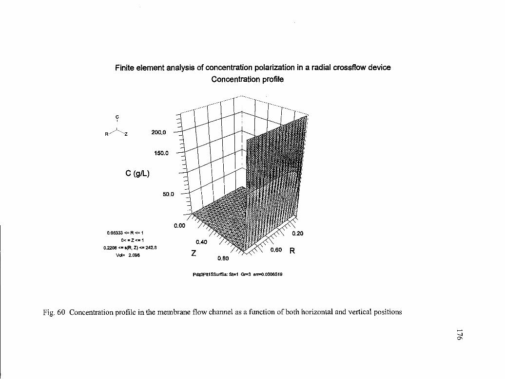
Finite element analysis of concentration polarization in a radial crossflow device
Concentration profile
C
R-'Z 200.0
C (gIL)
0.08333 <= R <= I
0< = Z <= I
0.2208 < s(R, Z) < 242.8
Vo1 2.098
150.0
50.0
0.00
z040
0.80
PdzOPftl5SurfSa: St=I Gr=3 ery=0.0008519
0.60 R
0.20
Fig. 60 Concentration profile in the membrane flow channel as a function of both horizontal and vertical positions

200.0
C)
O.O8333<X<=1
0.2771<f(Radius)<=242.8 .0.0
From (0.083,1) to (1,1)
Finite element analysis of concentration polarization in a radial crossflow deviceConcentration profile
Fig. 61 Development of concentration polarization along the radius direction.
Curves:
Area: 221.9
04/06/97. 18:55:14
0.40 0.60 0.80
Radius
PdzOMonOBEIev
a
I I I I I I I I

250
200
100
50
3.5E-10 - - - - 15E-10 - - - 7E-11
-
-
:/
--,./09 0.92 0.94 0.96 0.98
z
Fig. 62 Effect of effective diffusion coefficient on the thickness of the concentration boundary layer

3.5E-1 0
3E-1 0
2.5E-10
2E-10
t5E-10
IE-10
5E-11
0 II
0.00005 0.0001 0.00015 0.0002 0.00025 0.0003
Thickness of boundary layer (m)
Fig. 63 Linear relationship between the calculated boundary layer thickness and diffusion coefficient

180
(1.410 x 10⁶) can be determined from the slope of Fig. 63 and is compared favorably
with the one (1 .19 x 1 Ø6) calculated with Eq. (3) using Cm obtained by the finite element
analysis. Using the mass transfer coefficient and the value for Cm predicted in the finite
element analysis, the permeate flux calculated from Eq. (3) is 9.70 x 1 06 mis.
However, when a very small diffusion coefficient D is used, the concentration
boundary layer becomes very thin. More meshes are needed in the vicinity of the
membrane surface to obtain a quick and converged solution (Fig. 64). For a diffusion
coefficient of 7.0 x 10h1 m2/s, Eq. 47 was numerically solved using 21762 nodal points
and 10653 cells.
In summary, based on the physical property of the so lutes in the feed solution, the
finite element method can accurately simulate the development of concentration
polarization within the fluid flow channel and predict the BSA concentration (Cm) on the
membrane surface. This method can be used to estimate the mass transfer coefficient and
thickness of the concentration layer. It can also be used in the engineering analysis and
design of ultrafiltration processes, and should provide useful information for designing a
membrane filtration system.

Finite element analysis of concentration polarization in a radial crossflow device
Mesh generation for a small D
1.00
0.75
N 0.50
0.25
0.00
0.08333 <= R <= I
0< = Z <= I
Fig. 64 Mesh generation for D 7.0 x 10 m2Is
liii liii liii liii I
0.00 0.25 0.50 0.75 1.00
R
PdzOPItO7Grid: Gr=6 err=0.0006507

6. CONCLUSIONS
6.1 Audit of water consumption and waste water generation
The flow rates of waste water and the contribution of waste loads varied,
depending on the sources in the surimi processing line. Waste water from the gutting
operation and the first high speed dehydrator were the two major contributors of COD,
BOD5, and TS in the waste water. Although these two operations generated around 24%
of the total waste water, 60% of the total solid waste was generated in these two
operations. Overall, from the raw material stage to the frozen surimi stage of the
processing, for each kg of fish processed, approximately 5.7 L of waste water was
generated. About 0.05 1, 0.025, and 0.038 kg of COD, BOD5, and TS, respectively, were
generated for each kg of fish processed into frozen surimi. Although the waste water
generated in Subsystem 2 was almost twice as much as that in Subsystem 1, the flow rates
of solid wastes were similar. The total waste water generated in the processing plant was
750 m3 per day, with 473 m3 generated in the washing-dewatering processes.
6.2 Ohmic heating of surimi wash water
The ohmic heating study demonstrated the applicability of ohmic heating to
coagulate fish proteins and partially purify proteolytic enzymes from surimi wash water.
The study showed that temperature was a critical factor in controlling the degree of fish
protein coagulation and in preserving the activity of the proteases. The relationship
between temperature and heating time can be expressed using a second order polynomial
182

183
model, which indicates a linear heating rate (dT/dt) during ohmic heating. The electrical
conductivity of the wash water was predicted as 0.353 S/rn, which increased linearly with
the heating temperature at a rate of 0.0106 S/rn °C. After heating and centrifuging, the
residual solids (proteins, COD, TS, and TSS) concentration was found to follow Eq. (37).
Suspended solids were more susceptible to heat. At 40°C, more than 80% TSS were
removed, and at 60°C more than 90% TSS were removed. Reduction of protein
concentration was more than 80% at 60°C. Heating did not cause a complete coagulation
of proteins at 80°C. Some heat stable proteins, mainly those with molecular weights
below 20,000 Dalton, remained in the supernatant. Due to coagulation of the heat
sensitive fish proteins between 30 and 60°C, the specific activity of heat stable proteases
increased linearly with the heating temperature. At 60°C, the protease activity was
approximately 3 times that of the control, indicating that a partial purification of the
enzymes was achieved at this temperature. At temperatures above 60°C, a significant loss
of enzyme activity was observed due to heat denaturation. This temperature (60°C) may
be the highest at which the activity of the proteases is preserved, while coagulating the
majority of the fish proteins.
6.3 Microfiltration of surimi wash water
Microfiltration of surimi wash water started with high initial permeate fluxes, and
rapidly reached a steady state with permeate fluxes ranging from 20 to 22 L/m2hr, which
was twice the values reported by Jaouen et al.(1989 & 1990) and Jaouen and Querneneur
(1992). Although the characteristics of microfiltration membranes differed from each
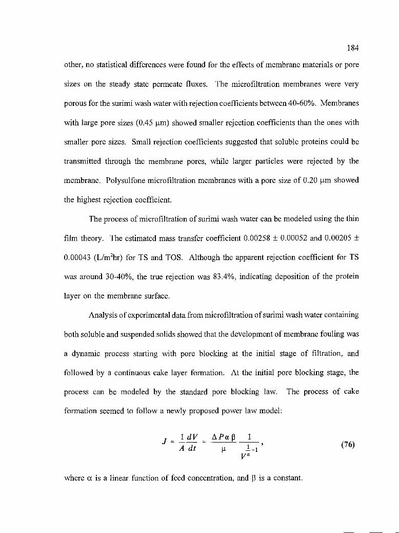
184
other, no statistical differences were found for the effects of membrane materials or pore
sizes on the steady state permeate fluxes. The microfiltration membranes were very
porous for the surimi wash water with rejection coefficients between 40-60%. Membranes
with large pore sizes (0.45 tm) showed smaller rejection coefficients than the ones with
smaller pore sizes. Small rejection coefficients suggested that soluble proteins could be
transmitted through the membrane pores, while larger particles were rejected by the
membrane. Polysulfone microfiltration membranes with a pore size of 0.20 jtm showed
the highest rejection coefficient.
The process of microfiltration of surimi wash water can be modeled using the thin
film theory. The estimated mass transfer coefficient 0.00258 ± 0.00052 and 0.00205 ±
0.00043 (L/m2hr) for TS and TOS. Although the apparent rejection coefficient for TS
was around 30-40%, the true rejection was 83.4%, indicating deposition of the protein
layer on the membrane surface.
Analysis of experimental data from microfiltration of surimi wash water containing
both soluble and suspended solids showed that the development of membrane fouling was
a dynamic process starting with pore blocking at the initial stage of filtration, and
followed by a continuous cake layer formation. At the initial pore blocking stage, the
process can be modeled by the standard pore blocking law. The process of cake
formation seemed to follow a newly proposed power law model:
ldV_ LPa13Adt F.L
(76)
v
where a. is a linear function of feed concentration, and 3 is a constant.

185
Although microfiltration membranes can be used to recover myofibrillar proteins,
the permeate flux is very low due to pore blocking and cake formation. The low
permeate flux may be an obstacle for a large scale application of microfiltration
technology to recover myofibrillar proteins from a large volume of industrial surimi wash
water. However, when ultrafiltration is used to treat the raw surimi wash water, the
presence of large particles may cause a rapid development of membrane fouling due to
the much higher pressure used in ultrafiltration (Cheryan, 1986). A pretreatment with
microfiltration or other technologies is necessary prior to ultrafiltration.
6.4 Finite element analysis of ultrafiltration of diluted BSA solutions
Finite element analysis with Pdease2D® can be used to simulate the development
of concentration polarization in the membrane flow channel during ultrafiltration of
diluted BSA solutions. The predicted BSA concentration (Cm) on the membrane surface
agreed with the theoretical value calculated based on the osmotic pressure model and the
values in the published literature.
Selection of effective diffusion coefficients affects the thickness of the
concentration boundary layer, but does not affect the prediction of Cm on the membrane
surface for a given permeate flux. When a very small diffusion coefficient is used in
finite element analysis, more meshes must be concentrated in the near vicinity of the
membrane surface to cope with the steep concentration gradient. For a given permeate
flux, linear relationship between diffusion coefficient and thickness of the concentration
boundary layer was observed, which is in agreement with the theory.

186
Finite element analysis can be used to predict the mass transfer coefficient, which
is an important parameter in engineering design and analysis of a membrane filtration
(RO/UF) process.
6.5 Summary and recommendations for future research
The objectives of this research project were accomplished. Detailed information
of water usage and waste water generation was gathered from a shore-based surimi
processing plant and the results can be applied to other shore-based surimi operations.
Water saving could be achieved by reducing the water supply in some unit operations,
such as heading, gutting, mincing. More studies are needed to improve the fish mince
washing efficiency.
The ohmic heating study has demonstrated its potential in coagulating fish proteins
and purifying proteases from Pacific whiting surimi wash water. More than 80% of fish
proteins could be removed from the wash water at temperatures above 60 °C. A 3-fold
increase in the protease activity was found in the wash water after heating to 60°C. More
studies should be done in applying this technology in extracting and purifying proteases
from Pacific whiting wash water.
Microfiltration was used to recover myofibrillar proteins from surimi wash water.
Under the test conditions, the permeate fluxes ranged from 20-22 L/m2hr for four different
membranes regardless of the different pore size and membrane materials. This study
demonstrated that membrane fouling, which dramatically reduced the permeate flux, was
caused by initial pore blocking and continuous cake formation. The cake resistance was

187
dominant throughout the pseudo-steady state filtration. A new continuous cake formation
model was proposed and verified. Future studies are needed to develop an innovative
membrane filtration process that can substantially reduce the cake formation on the
membrane surface.
A new computer simulation method based on finite element analysis was used to
accurately predict the mass transfer coefficient and solute concentration on the membrane
surface during ultrafiltration of a single component protein solution. This method could
be used in engineering design and analysis of membrane filtration process (ultrafiltration
and reverse osmosis).

7. NOMENCLATURES
Ae effective electric conducting area of the electrodes (m2)
Am effective membrane filtration areas (m2)
B constant
Bi constant (m/Vp), i/L
BOD biological oxygen demand (gIL)
C solids (protein, COD, TS, and TSS) concentration (gIL)
Cb feed concentration (g/L)
Cm solute concentration on membrane surface (g/L)
C permeate concentration (g/L)
COD chemical oxygen demand (g/L)
d pore diameter (tm)
d0 initial pore diameter (.im)
d diameter of particles (m)
d pore diameter at time t (iim)
D solute diffusion coefficient (m2/s)
h thickness of membrane (m)
H height of a plate-and-frame membrane filter (m)
I electric current (A)
J permeate flux (L/m2s)
J0 initial permeate flux (L/m2s)
permeate flux at time t (LIm2s)
188
k mass transfer coefficient (mis)
K constant, equal to 1/(J0Ae)
K effective ohmic heating device coefficient
thickness of cake layer, m
L distance between two electrodes (m)
m5 amount of solids deposited on the internal walls of pores (kg/L)
total number of pore of membrane
p pressure (Pa)
P pressure (Pa)
Q flow rate of water or waste water (L/s)
r radius (m)
ra apparent rejection coefficient
r true rejection coefficient
R radius of a radial crossflow membrane filter (m)
R cake layer resistance (1/rn)
Re Reynolds number (1/rn)
Rm resistance of a clean membrane (1/rn)
specific cake resistance (11m4)
R total resistance (1/rn)
Sc Schmidt number
Sh Sherwood number
t filtration time (s)
189

t reference time point at which flow stabilized (s)
I heating temperature at time t (°C)
TS total solids (giL)
TSS total suspended solids (giL)
u horizontal velocity component (mis)
v vertical velocity component (mis)
V permeate volume (L)
V permeate volume at t, (L)
initial pore volume (m3)
Ve electric voltage (V)
a constant, linear function of C
constant
thickness of concentration polarization (m)
porosity of membrane
shear rate (us)
dimensionless vertical distance
viscosity of the feed (Pa.$)
7t osmotic pressure (Pa)
density of solids deposited on the pore walls (kg/rn3)
apparent electrical conductivity (S/rn)
t tortuosity of membrane
constant
190
REFERENCES
Anonymous. 1994. Industrial sewer account - monthly billing report. City of Albany,Oregon.
An, H., Peter, M. Y., Seymour, T. A., and Morrissey, M. T. 1995. Isolation andactivation of Cathepsin L- commplex from Pacific whiting (Merlucciusproductus).J. Agric. Food Chem. 43, 337-330.
An, H., Weerasinghe, V., Seymour, T. A., and Morrissey, M. T. 1994a. Cathepsindegradation of Pacific whiting surimi proteins. J. Food Sci. 59, 1013-1017, 1033.
An, H., Seymour, T. A., Wu, J, and Morrissey, M. T. 1994b. Assay systems andcharacterization of Pacific whiting. J. Food Sci. 59, 277-281.
AOAC, 1995. AOAC Official Method 938.08. In Official Methods of Analysis ofAOAC International, 16th Edition, (P. Cunniff, ed). AOAC International,Arlington, VI.
Babbitt, J., Repond, K., Hardy, A., Zetterling, T., and Swafford, T. C. 1985. Effect ofwashing on the composition and functional stability of minced pollock flesh. InProceedings ofInternational Symposium on Engineered Seafood Including Surimi.Nov. 19-21, 1985. Seattle, WA, R. E. Martin and R. L. Collette (Eds), NationalFishery Institute, Washington, DC, p 117-128.
Baker, A. J. and Pepper, D. W. 1991. Finite Elements 1-2-3. McGraw-Hill, Inc. NewYork.
Belfort, G. Davis, R. H. and Zydney, A. L. 1994. The behavior of suspensions andmacromolecular solutions in crossflow microfiltration. J. Memb. Sci. 96: 1-58.
Benjakul, J., Seymour, T. A., Morrissey, M. T., and An, H. A. 1996. Proteinase inPacific whiting surimi wash water: identification and characterization. J. Food Sci.61: 1165-1170.
Berman, A. S. 1953. Laminar flow in channels with porous walls. J. Applied. Phys.(24): 1232-1235.
Bhattacharyya, D., William, M., Ray, R. J., and McCray, S. B. 1992. Chapter 23Design. In Membrane Handbook, (W. S. W. Ho and K. K. Sirkar, eds), VanNostrand Reinhold, New York.
191
Biotol, 1992. Product Recovery in Bioprocess Technology, published on behalf of OpenUniversiteit and Thames Polytechnic, Butterworth-Heinemann Ltd.
192
Biss, C. H., Coombes, S. A. and Skudder, P. J. 1989. The development and applicationof ohmic heating for the continuous processing of particulate food stuffs. InProcess Engineering in the Food Industry, (R. W. Field and J. A. Howell, eds),p. 17-27, Elsevier, London.
Blanpain, P., Hermia, J., and Lenoel, M. 1993. Mechanisms governing permeate fluxand protein rejection in the microfiltration of beer with a Cyclopore membrane.J. Membrane Sci. (84): 37-5 1.
Blatt, W. F., David, A., Michaels, A. S., and Nelson, L. 1970. Solute polarization andcake formation in membrane ultrafiltration: Causes, consequence, and controltechniques, In Membrane Science and Technology, (J. E. Flinn, ed), Plenum Press,New York.
Bouchard, C. R., Carreau, P. J., Matsuura, T., and Sourirajan, S. 1994. Modeling ofultrafiltration: prediction of concentration polarization effects. J. Membrane Sci.(97) 215-229.
Bough, W. A., Landles, D. R., Miller, J, Young, C. T., and McWhorter. 1975.Utilization of chitosan for recovery of coagulated by-products from foodprocessing wastes and treatment systems. In Proceedings of the Sixth NationalSymposium on Food Processing Wastes, April 9-11, 1975. Madison, WI.
Bowen, W. R. 1993. Understanding flux patterns in membrane processing of proteinsolutions and suspensions. Trends in Biotech. (11): 45 1-460.
Bowen, W. R. and Gan, Q. 1991. Properties of microfiltration membranes: flux lossduring constant pressure permeation of bovine serum albumin. Biotech. andBioeng. (38): 688-696.
Bowen, W. R. and Gan, Q. 1992. Properties of microfiltration membranes: the effectsof adsorption and shear on the recovery of an enzyme. Biotech. And Bioeng.(40): 49 1-497.
Bowen, W. R. and Hall, N. J. 1995. Properties of microfiltration membranes:mechanisms of flux loss in the recovery of an enzyme. Biotech. And Bioeng.(46): 28-35.
Brian, P. L. T. 1965. Concentration polarization in reverse osmosis desalination withvariable flux and incomplete salt rejection. md. Eng. Chem. Fundam. (4) 439-445.
Brian, P. L. T. 1966. Mass transport in reverse osmosis. In Desalination by ReverseOsmosis, (U. Merten, ed), MIT Press, Cambridge, MA.

de Alwis, A. A. P., and Fryer, P. J. 1990. The use of direct resistance heating techniquesin the food industry. J. Food Eng. 11, 3-27.
193
Chao, A. C., Machemehi, J. L., and Galarrange, E. 1980. Ultrafiltration treatment ofseafood processing wasterwaters. In Proc. 35th Industrial Waste Concerence,Purdue University, p 560-570.
Chao, A. C., Tzou, L, and Young, C. T. 1983. Recovery and application of solids fromcrab-processing wastewater. In Proc. 38th Industrial Waste Conference, PurdueUniversity, p 829-838.
Chao, A. C. , Tzou, L., and Green, D., 1984. Modeling of ultrafiltration for treatingfishery wastewaters. In Proc. 39th Industrial Wastes Conference, PurdueUniversity, p 555-563.
Cheftel, J. C., Cuq, J. L., and Lorient, D. 1985. Amino acids, peptides, and proteins.In Food Chemistry, (0. R. Fennema, ed), Marcel Dekker, Inc., p. 245-369.
Cheryan, M. 1986. Ultrafiltration Handbook. Technomic Publishing Co, Inc. Lancaster,PA.
Cheryan, M. And Merin, U. 1980. A study of the fouling phenomena duringultrafiltration of cottage cheese whey. In Ultrafiltration membranes andApplications, (A. R. Cooper, ed), Pleunum Press, New York, p. 619.
CH2M Hill. 1993. Reviews of environmental management options at Inland QuickFreeze Albany Oregon. Prepared for Pacific Power & Light Company.
Cocci, A. A., Wilson, D. R., and Landine, R. C. 1991. Anaerobic treatment of clamprocessing wastewater. In Proceedings of Seafood Environmental Summit- APortion of the Seafood and the Environment Symposium, Raleigh, NC.
Colton, C. K., Henderson, L. W. Ford, C. A. 1975. Kinetics of hemodiafiltration. I. InVitro transport characteristics of a hollow-fiber blood ultrafilter. J. Lab. Clin.Med. 85: 355
Cowan, J. A. C., MacTavish, F., Brouckaert, C. J. and Jacobs, E. P. 1992. Membranetreatment strategies for red meat abattoir effluents. Water. Sci. Tech. 25(10): 137-148.
Dalrymple, C. W. 1994. Use of electrocoagulation for wastewater treatment. In:Wastewater Technology Conference and Exhibition. Conference Proceedings.Hotel Vancouver, Vancouver, British Columbia, Canada.

194
Drukker, W., Parsons, F. M., and Maher, J. F. 1983. Replacement of renal function bydialysis. Martinus Nijhof, Boston.
Dziezak, J. D. 1990. Membrane separation technology offers processors ultimatedpotential. Food Tech. (9): 108-113).
Eckstein, E. C., Bailey, D. G., and Shapiro, A. H. 1977. Self-diffusion of particles inshear flow of a suspension. J. Fluid. Mech. 79: 191.
Edwards, R. H. and Kohier, G. 0. 1981. Heating of proteinaceous liquids. US. Patent No4,421,682.
Forsht, E. H. 1974. Development document for effluent limitation guidelines and newsources performance standards for the catfish, crab, shrimp and tuna segment ofthe canned and preserved seafood processing source categories. EPA-4407 1-74-0290-1, U.S. Environmental Protection Agency, Washington, DC.
Fresenius, W., Schneider, W., Bohnke, B., and Poppingaus, K. 1989. Waste watertechnology - origin, collection, treatment and analysis of waste water. Springer-Verlag, Berlin and Heidelberg, Germany.
Ganguly, S. And Bhattacharya, P. K. Development of concentration profile andprediction of flux for ultrafiltration in a radial cross-flow cell. J. Membrane Sci.(97): 185-198.
Gekas, V. And Halistrom, B. 1987. Mass transfer in the membrane concentration layerunder turbulent flow. J. Membrane Sci. 30: 153.
Gibbs, C. R. 1979. Introduction to chemical oxygen demand. Technical informationseries - Booklet No. 8. Hach Chemical Co. Loveland, Co.
Goel, V., Accomazzo, M. A., Dileo, A. J., Meier, P., Pitt, A., and Pluskal, M. 1992.Dead-end microfiltration: application, design, and cost. In Membrane Handbook,(W. S. W. Ho and K. K. Sirkar, eds), Van Nostrand Reinhold, New York.
Greenberg, A. E., Trussell, R. R., Clesceri, L. S. 1980. Standard methods for theexamination of water and waste water. 15th Edition. APHA (American PublicHealth Association), AWWA (American Pollution Water Works Association), andWPCF (Water Pollution Control Federation). Washington, D.C.
Harrison, T. D., Boardman, G. D., and Flick, G. J., 1992. Characterization and treatmentof wastes from blue crab processing facilities. In Proc. 42th Industrial WasteConference, Purdue University, p 775-788.

195
Hopkins, K. 1983. Case histories: pretreatment of poultry processing wastewater. In:Proc. 38th Industrial Waste Conference, Purdue University, West Lafayette,Indiana.
Huang, L. Chen, Y., and Morrissey, 1996. Coagulation of fish proteins from frozen fishmince wash water by ohmic heating. J. Food Proc. Eng. (In press).
Huang, L. and Morrissey, M. T. 1 997a. Application of ohmic heating to coagulateproteins and partially concentrate proteolytic enzymes in surimi wash water.Submitted to J. of Aquatic Food Product Technology.
Huang, L. And Morrissey, M. T. .1997b. Fouling of membranes during microfiltrationof surimi wash water: roles of pore blocking and surface cake formation.Submitted to J. of Membrane Science.
Huang, L. Santos, M. Singh, P. R., and Morrissey, M. 1997. Characterization of wastewater from the surimi processing industry. To be submitted to J of Aquatic FoodProduct Technology.
Hultin, H. 0. 1985. Characteristics of muscle tissue. In Food Chemistry, 2nd edition,(0. R. Fennema, ed). Marcel Dekker, Inc. New York and Basel.
Ingham, K. C., Busby, T. F. Sahiestrom, Y., and Castino, F. 1980. Separation of macromolecules by ultrafiltration: Influence of protein adsorption, protein-proteininteraction and concentration polarization, In Ultrafiltration membranes andApplications, (A. R. Cooper, ed), Pleunum Press, New York, p. 141.
Iritani, E., Hayashi, T., and Murase, T. 1991. Analysis of filtration mechanism ofcrossflow upward and downward ultrafiltration. J. Chem Eng. Japan (24): 3 9-44.
Ismond, A. 1994. How to do a seafood processing plant water, waste, and wastewateraudit. Aqua-Terra Consultants. Seattle, WA.
Ismond, A. 1997. Personal communication. Aqua-Terra Consultants. March 1997.Seattle, WA.
Jaouen, P., Bothorel, M., and Quemeneur, F. 1989. Recovery of soluble proteins bymembrane separation process: Performances and membrane cleaning. InPreprints: 6th International Symposium on Synthetic Membranes in Science andTechnology, September 4-8, 1989, Thubingen, Germany.
Jaouen, P., Bothorel, M., and Quemeneur, F. 1990. Treatment of seafood processingeffluents through microporous membranes - applications and prospects. In Proc.of International Congress on Membranes and Membrane Process. Chicago, USA.

196
Jaouen, P. and Quemeneur, F. 1992. Membrane filtration for waste-water proteinrecovery. In Fish Processing Technology, (G. M. Hall, ed), Blackie Academic &Professional, published in North America by VCH Publishers, Inc., New York.
Johnson, H. M. 1996. 1996 Annual report on the United States Seafood Industry. H.M. Johnson & Associates.
Johnson, R. A. and Gallanger, S. M. 1984. Use of coagulants to treat seafood processignwastewaters. J. Water. Pollution Control Federation (56):970-976.
Kasper, D. R. and Reichenberger, J. C. 1983. Use of polymers in the coagulationprocess. In Proc. of A WMA Seminar on Use of Organic Polyelectrolytes in WateTreatment, Las Vegas, NE.
Kawakatsu, T., Nakao, S., and Kimura, S. 1993. Effect of size and compressibility ofsuspended particles and surface pore size of membrane on flux in crossflowfiltration. J. Membrane Sci. (81): 173-190.
Kleinstreuer, C. and Paller, M. S. 1983. Laminar dilute suspension flows in plate-and-frame ultrafiltration units. AICHE Journal (28) 529-533.
Knorr, D. 1991. Recovery and utilization of chitin and chitosan in food processing wastemanagement. Food Tech. (1): 114-122.
Koiff, W. J. and Berk, H. T. 1944. The artificial kidney: a dialyzer with a great area.Acta Med. Scan. 117:121-134.
Laemmli, U. K. 1970. Cleavage of structural protein during the assembly of the headof bacteriophage T4. Nature 227: 680-685.
Lebrun, R. E., Bouchard, C. R., Rollin, A. L., Matsuura, T., and Sourirajan, 5. 1989.Computer simulation of membrane separation processes. Chemical Eng. Sci. (44)3 13-320.
Lee, C. M. 1984. Surimi process technology. Food Tech. (11): 69-80.
Lee, C. M. 1985. A pilot plant study of surimi-making properties of red hake. Paper No.20., presented at International Symposium on Engineered Seafood IncludingSurimi, Seattle, WA., Nov 19-21.
Lee, C. M., 1986. Surimi manifacturing and fabrication of surimi-based products. FoodTech. (3):115-124.
197
Lee, D. N. and Merson, R. L. 1975. Examination of cottage cheese whey protein byscanning electron microscopy: Relationship to membrane fouling duringultrafiltration. J. Dairy Sci. 48(10) 1423.
Li, N. N. 1984. Membrane processes. In Perry 's Chemical Engineers' Handbook, (R.H. Perry, D. W. Green, and J. 0. Maloney, eds). McGraw-Hill chemicalengineering series. McGraw-Hill, Inc., New York.
Lin, T. M., Park, J. W., and Morrissey, M. T. 1995. Recovered protein andreconditioned water from surimi processing waste. J. Food Sci. 50(1):6-9.
Lin, T. M. 1996. Solubility and structure of fish myofibrillar proteins as affected byprocessing parameters. Doctoral Thesis. Department of Food Science andTechnology, Oregon State University. Corvallis, OR.
Lind, C. 1995. A coagulant road map. Public Work (3):36-38.
Longsdale, H. K. 1983. Reverse osmosis. In Synthetic Membranes. Science,Engineering and Application, (P. M. Bungay, H. K. Longsdale, and M. N. DePinho, eds). NATO ASI Series. Series C, Mathematical and physical sciences;Vol. 181.
Lowry, 0. H., Rosebrough, N. J., Farr, A. L., and Randall, R. J. 1951. Proteinmeasurement with Folin phenol reagent. J. Biol. Chem. (193):256-257.
Ludlow, M. 1997. Personal communication. Natural Biopolymers, Inc. January1997. Raymond, WA.
Madsen, R. F. 1977. Hyperfiltration and Ultrafiltration in plate-and-frame systems.Elsevier Scientific Publishing Co.
Mannapperuma, J. D., Mate, J. I., and Singh, R. P. 1993. Reduction of environmentalimpact and energy use through water recycling and by-product recovery in foodprocessing, final report prepared for the California Institute for Energy Efficiency.Department of Agricultural Engineering, University of California, Davis. Davis,CA.
Marshall, A. D., Munro, P. A., and Tragardh, G. 1991. The effect of protein foulinginmicrofiltration and ultrafiltration on permeate flux, protein retention andselectivity: A literature review. Desalination 91: 65-108.
Martin, D. W. 1983. Membranes. In Harper's Review of Biochemistry, 19th edition, (D.W. Martin, Jr., P. A. Mayes, and V. W. Rodwell, eds), Lange MedicalPublications, Los Altos, CA.

198
Mate, J. I. 1992. Accounting and simulation of waste water use and recycling in foodprocessing. M.S. Thesis. Department of Agricultural Engineering. University ofCalifornia, Davis. Davis, CA 95616.
Matsumoto, J. J. 1978. Minced fish technology and its potential for developingcountries. In Proceedings on Fish Utilization Technology and Marketing, Vol. 18,Sec III, p. 267. Indo-Pacific Fishery Commision. Bankok. Thailand.
Matthiasson, E. 1983. The role of macromolecular adsorption in fouling of ultrafiltrationmembranes. J. Membrane Sci. 16: 23-36.
Mikkelson, K. A. And Lowery, K. W. 1992. Desogning a sequential batch reactorsystem for the treatment of high strength meat processing wastewater. In Proc.47th Industrial Waste Conference, Purdue University, West Lafayette, Indiana.
Mir, L., Michael, S. L., and Goel, V. 1 992a. Crossflow microfiltration: application,design, and cost. In Membrane Handbook, (W. S. W. Ho and K. K. Sirkar, eds),Van Nostrand Reinhold, New York.
Mir, L., Michael, S. L. Goel, V., and Kaiser, R., 1992. Crossflow microfiltration:applications, design, and cost. In Membrane Handbook, (W. S. W. Ho and K. K.Sirkar, eds), Van Nostrand Reinhold, New York.
Miyata, Y. 1984. Concentration of protein from the wash water of red meat fish byultrafiltration membrane. Bull. of the Japan. Soci. of Sci. Fish. 50 (4): 659-663.
Mohr. C. M., Engelgau, D. E., Leeper, S. A., and Charboneau, B. L. 1989. Membraneapplications and research in food processing. Noyes Data Corp. Park Ridge, NJ.
Muhuriji, M., Faggard, G., Van Der Mast, V., and Iamai, H. 1989. Jeddah I RO plant -Phase 115 MGD reverse osmosis plant. Desalination 76: 75.
Mulder, M. 1990. Basic Principles of Membrane Technology. Kiuwer AcademicPublishers. The Netherlands.
Murase, T., Ohn, T., and Kimtat, K. 1995. Filtrate flux in crossflow microfiltration ofdilute suspension forming a highly compressible fouling cake-layer. J. MembraneSci. (108): 121-128
Nakao, S. Wijmans, J. G., and Smolders, C. A. 1986. Resistance to the permeate fluxin unstirred ultrafiltration filtration of dissolved macromolecular solutions. J.
Membrane Sci. (26): 165-178.

199
Nilson, J. L. 1990. Protein fouling of UF membranes: causes and consequences. J.
Membrane Sci. 52: 121-142.
Ninomiya, K., Ookawa, T., Tsuchiya, T., and Matsumoto. 1985. Recovery of watersoluble protein in waste wash water of fish processing plants of Ultrafiltration.Bull, of the Japan. Soci. of Sci. Fish. 51(7): 1133-1138.
Okada, M. 1992. History of surimi technology. In Surimi Technology, (T. C., Lanierand C. M., Lee, eds), Marcel Dekker, Inc. New York, pp. 3-39.
Pacheco-Aguilar, R., Crawford, D. L., and Lampila, L. E. 1989. Procedures for theefficient washing of minced whiting (Merluccius products) flesh for surimiproduction. J. Food Sci. 54: 248-252.
Palaniappan, S. and Sastry, S. K. 1991a. Electrical conductivity of selected solid foodsduring ohmic heating. J. Food Process Eng. 14, 221-236.
Palaniappan, S. and Sastry, S. K. 1991b. Electrical conductivity of selected juices:Influences of temperature, solids content, applied voltage, and particle size. J.
Food Process Eng. 14, 247-260.
Park, J. W. 1997. Personal communication. March 1997. Oregon State UniversitySeafood Laboratory, Astoria, OR.
Paulson, D. J., Wilson, R. L., and Spatz, D. D. 1984. Crossflow membrane technologyand its applications. Food Tech. (12): 77-111.
Pearce, R. J. 1992. Whey protein recovery and whey protein fractionation. In Whey andlactose processing, (J. G. Zalow, ed)., Elsevier Science Publishing Co. Inc., NewYork.
Perry, R. H., Green, D. W., and Maloney, J. 0. 1984. Perry's Chemical Engineers'Handbook. McGraw-Hill, Inc., New York.
Peters, G. 1997. Personal communications. Alyeska Seafoods. Dutch Harbor, Alaska.
Petersons, L. D. 1990. Product recovery from surimi wash water. In Making Profitsout of Seafood Wastes: Proceedings of the International Conference on Fish By-Product, (S. Keller, ed), Anchorage, Alaska.
Porter, M. C. 1972. Concentration polarization with membrane ultrafiltration. md. Eng.Chem. Prod. Res. Dev, 11: 234.

200
Porter, M. C. 1979. Membrane filtration. In Handbook of Separation techniques forChemical Enggineers, (P. A. Schweitzer, ed). McGraw-Hill
Radtke, H. 1995. Windows on Pacific whiting: An economic success story for Oregon'sfishing industry. Oregon Coastal Zone Management Association, Newport, OR.
Rautenbach, R. And Albrecht, R. 1989. Membrane Process. John Willey & Sons.
Redkar, S. G. and Davis,R. H. 1993. Crossflow microfiltration of yeast suspensions intubular filters, Biotechnol. Prog. (9) 625-634.
Regier, W. L., Ernst, R. C., and Hale, M. B. 1985. Processing requirements for thepreparation of minced intermediates or surimi from menhaden. In Proceedings ofthe International Symposium On Engineered Seafood Including Surimi. November19-21, 1985. Seattle, WA, R. F. Martin and R. L. Collette (Eds), NationalFisheries Institute, Washington, D.C., pp 129-140.
Renner, E. and Abd El-Salam, M. H. 1991 Application of Ultrafiltration in the DairyIndustry. Elsevier Science Publishers Ltd.
Rusten, B., Eikebrokk, B., and Thorvaldsen, G. 1990. Coagulation as pretreatment offood industry wastewater. Wat. Sci. Tech. 22 (9): 1-8.
Sandu, C., and Singh, R. K. 1991. Energy increase in operation and cleaning due to heatexchanger fouling in milk pasteurization. Food Tech. 45(12), 84-91.
Sastry, K. S. and Palaniappan, S. 1992. Ohmic heating of liquid-particle mixtures. FoodTech. 46(12), 64-67.
Seymour, T. A., Morrissey, M. T., Peters, M. Y., and An, H. 1994. Purification andcharacterization of Pacific whiting proteases. J. Agric. Food Chem. 42, 2421-2427.
Shoji, T., Nakajima, M., Nabetani, H., Ohtani, T., and Watanabe, A. 1988. Effect ofpore size of ceramic support on the self-rejection characteristics of the dynamicmembrane formed with water soluble proteins in waste water. NipponNogeikagaku Kaishi 62 (7): 1055-1060.
Singh,R. And Laurence, R. L. 1979. Influence of slip velocity at membrane surface onultrafiltration performance: I. Channel flow system. mt. J. Heat Mass Transfer(22) 721.
Stirling, R. 1987. Ohmic heating - a new process for the food industry. Power Eng.J. 6, 365-369.
201
Suki, A., Fane, A. G. F., and Fell, C. J. D. 1984. Flux decline in protein ultrafiltration.J. Memb. Sci. 21: 269-283.
Swafford. T. C., Babbitt, J, Reppond, K., Hardy, A., Riley, C. C., and Zetterling, T. K.A. 1985. Surimi process yield improvement and quality contribution bycentrifuging. In Proceedings of the International Symposium On EngineeredSeafood Including Surimi. November 19-21, 1985. Settle, WA, R. B. Martin andR. L. Collette (Eds), National Fisheries Institute, Washington, D.C., pp483-496.
Tanaka, T., Kamimura, R., Itoh, K., and Nakanishi, K. 1993. Factors affecting theperformance of crossflow filtration of yeast cell suspensions. Biotech. AndBioeng. (41): 617-624.
Toyoda, K., Kimura, I., Fujita, T., Noguchi, S. F., and Lee, M. 1992. The surimimanufacturing process. In: Surimi Technology, T. C., Lanier and C. M., Lee(Eds), Marcel Dekker, Inc. New York, pp. 79-112.
U.S. Environmental Protection Agency 1967. Evaluation of Waste Disposal Practices ofAlaskan Seafood Processors. Office of Enforcement, EPA-33012-75-00l,Washington.
Van den berg, G. B. And Smolders, C. A. 1988. Flux decline in membrane processes.Filtration & Filtration (March/April): 115-121.
Viker, V. L., Colton, C. K., and Smith, K. A. 1981. The osmotic pressure ofconcentrated protein solutions: Analysis of concentration polarization and solutionpH dependence for bovine serum albumin in saline solution. J. Colloid InterfaceSci. (79) 548.
Viker, V. L., Colton, C. K., Smith, K. A., and Green, D. L. 1984. The osmotic pressureof concentrated protein and lipoprotein solutions and its significance toultrafiltration. J. Membrane Sci. (20) 63.
Watanabe, T. 1974. Treatment of waste solutions containing animal blood. Japan KokaiNo. 74, 79,052.
Watanabe, H., Takai, R., Sekigawa, A., and Hasegawa, H. 1982. An estimation of theamount of protein lost in the effluent from frozen surimi manufacture. Bull. Jap.Soc. Fish. 48: 869.
Watanabe, A., Ohtani, T., Horikita, H., Ohya, H., and Kimura, S. 1986. Recovery ofsoluble protein from fish jelly processing with self-rejection dynamic membrane.In Food Engineering Process Applications, (L. Le Maguer and P. Jelen, eds), Vol2. P. 225-236.

202
Watanabe, A., Shoji, T., Nakajima, M., Nabetani, H., and Ohtani, T. 1988.Electronmicroscopic observation of self-rejection type dynamic membrane formedwith water soluble proteins in waste water from fish paste process. NipponNogeikagaku Kaishi 62 (7) 106 1-1066.
Wojcik, C. 1983. Desalination of water in Saudi Arabia by reverse osmosis performancestudy. Desalination 46:17.
Zydney, A. L. And Colton, C. K. 1986. A concentration polarization model for thefilterate flux in cross-flow microfiltration of particulate suspensions. Chem. Eng.Commun. 47: 1-21.